copy of chapter07 12 - hal.archives-ouvertes.fr
TRANSCRIPT

HAL Id: hal-00408305https://hal.archives-ouvertes.fr/hal-00408305
Submitted on 30 Jul 2009
HAL is a multi-disciplinary open accessarchive for the deposit and dissemination of sci-entific research documents, whether they are pub-lished or not. The documents may come fromteaching and research institutions in France orabroad, or from public or private research centers.
L’archive ouverte pluridisciplinaire HAL, estdestinée au dépôt et à la diffusion de documentsscientifiques de niveau recherche, publiés ou non,émanant des établissements d’enseignement et derecherche français ou étrangers, des laboratoirespublics ou privés.
Assessment and Conservation of Forest Biodiversity inthe Western Ghats of Karnataka, India. 2. Assessment
of Tree Biodiversity, Logging Impact and GeneralDiscussion.
B.R. Ramesh, M.H. Swaminath, Santhoshagouda Patil, S. Aravajy, ClaireElouard
To cite this version:B.R. Ramesh, M.H. Swaminath, Santhoshagouda Patil, S. Aravajy, Claire Elouard. Assessment andConservation of Forest Biodiversity in the Western Ghats of Karnataka, India. 2. Assessment of TreeBiodiversity, Logging Impact and General Discussion.. Institut Français de Pondichéry, pp. 65-121,2009, Pondy Papers in Ecology no. 7, Head of Ecology Department, Institut Français de Pondichéry,e-mail: [email protected]. �hal-00408305�
INSTITUTS FRANÇAIS DE RECHERCHE EN INDE FRENCH RESEARCH INSTITUTES IN INDIA
PONDY PAPERS IN ECOLOGY
ASSESSMENT AND CONSERVATION OF FOREST
BIODIVERSITY IN THE WESTERN GHATS OF
KARNATAKA, INDIA. 2. ASSESSMENT OF TREE
BIODIVERSITY, LOGGING IMPACT AND GENERAL
DISCUSSION.
B.R. Ramesh
M.H. Swaminath
Santhoshagouda Patil
S. Aravajy
Claire Elouard
INST1TUT FRANÇAIS DE PONDICHÉRY FRENCH INSTITUTE PONDICHERRY 7
PONDY PAPERS IN ECOLOGY No. 7
Assessment and Conservation of Forest Biodiversity in the Western Ghats of Karnataka, India.
2. Assessment of Tree Biodiversity, Logging Impact and General Discussion
B. R. Ramesh M. H. Swaminath
Santhoshagouda Patil S. Aravajy
Claire Elouard
INSTITUT FRANÇAIS DE PONDICHÉRY

The Institut français de Pondichéry (IFP) or French Institute of Pondicherry, is a financially autonomous research institution under the dual tutelage of the French Ministry of Foreign and European Affairs (MAEE) and the French National Centre for Scientific Research (CNRS). It was established in 1955 under the terms agreed to in the Treaty of Cession between the Indian and French governments. It has three basic missions: research, expertise and training in human and social sciences and ecology in South and South-East Asia. More specifically, its domains of interest include Indian cultural knowledge and heritage (Sanskrit language and literature, history of religions, Tamil studies, ..), contemporary social dynamics (in the areas of health, economics and environment) and the natural ecosystems of South India (sustainable management of biodiversity). French Institute of Pondicherry, UMIFRE 21 CNRS-MAEE, 11, St. Louis Street, P.B. 33, Pondicherry 605001, INDIA Tel: 91-413-2334168; Fax: 91-413-2339534 Email: [email protected] Website: http://www.ifpindia.org
Authors B. R. Ramesh, Santhoshagouda Patil, S. Aravajy and Claire Elouard are from the French Institute of Pondicherry. M. H. Swaminath is from the Karnataka Forest Department, Bangalore.
This volume is part of a report published in collaboration with the Karnataka Forest Department under reference: Ramesh, B. R. and Swaminath, M. H., 1999. Assessment and conservation of forest biodiversity in the Western Ghats of Karnataka, India. Final report of a project funded by the Fonds Français de l'Environnement Mondial, convention n° 12-645-01-501-0. 126 pp.
© Institut français de Pondichéry, 2009 Typeset by Mr. G. Jayapalan
Summary PPE volumes 6 and 7 are parts of a project report published in 1999 in collaboration with the Karnataka Forest Department on the assessment and conservation of forest biodiversity in the Western Ghats of Karnataka. Project objectives and study area are introduced in the first volume (PPE 6). The present volume reports i) an assessment of forest biodiversity and its relationships with regional bioclimate and anthropogenic pressure from a network of 96 1-ha sampling plots, and ii) an in-depth study of impact of selective logging on the low elevation wet evergreen forest, which revealed that 30-40 years between successive harvests is the minimum period to allow the forest to recover. Conservation values maps and recommendations for forest management are then discussed from results of the whole project. Keywords: Biodiversity, Karnataka, India, logging impact, tropical forests, Western Ghats.
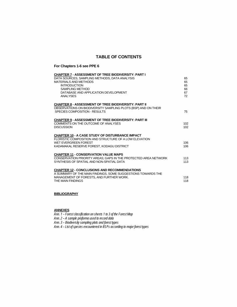
TABLE OF CONTENTS For Chapters 1-6 see PPE 6 CHAPTER 7 - ASSESSMENT OF TREE BIODIVERSITY: PART I DATA SOURCES, SAMPLING METHODS, DATA ANALYSIS 65 MATERIALS AND METHODS 65
INTRODUCTION 65 SAMPLING METHOD 66 DATABASE AND APPLICATION DEVELOPMENT 67 ANALYSES 72
CHAPTER 8 - ASSESSMENT OF TREE BIODIVERSITY: PART II OBSERVATIONS ON BIODIVERSITY SAMPLING PLOTS (BSP) AND ON THEIR SPECIES COMPOSITION - RESULTS 75 CHAPTER 9 - ASSESSMENT OF TREE BIODIVERSITY: PART III COMMENTS ON THE OUTCOME OF ANALYSES 102 DISCUSSION 102 CHAPTER 10 - A CASE STUDY OF DISTURBANCE IMPACT FLORISTIC COMPOSITION AND STRUCTURE OF A LOW ELEVATION WET EVERGREEN FOREST 106 KADAMAKAL RESERVE FOREST, KODAGU DISTRICT 106 CHAPTER 11 - CONSERVATION VALUE MAPS CONSERVATION PRIORITY AREAS; GAPS IN THE PROTECTED AREA NETWORK 113 SYNTHESIS OF SPATIAL AND NON-SPATIAL DATA 113 CHAPTER 12 - CONCLUSIONS AND RECOMMENDATIONS A SUMMARY OF THE MAIN FINDINGS, SOME SUGGESTIONS TOWARDS THE MANAGEMENT OF FORESTS, AND FURTHER WORK. 118 THE MAIN FINDINGS 118 BIBLIOGRAPHY
ANNEXES Ann. 1 – Forest classification on sheets 1 to 3 of the Forest Map Ann. 2 – A sample proforma used to record data Ann. 3 – Biodiversity sampling plots and forest types Ann. 4 – List of species encountered in BSPs according to major forest types
65
Assessment of tree biodiversity: Part I Data sources, sampling methods, data analysis
Materials and Methods
Introduction
Biodiversity (BD) has been defined as the variability among living organisms and the ecological systems of which they are part. Thus the term includes not only the species themselves, but also the roles they play in the ecosystem and the relationships between them. BD can be considered at genetic, taxonomic and ecosystem levels, and variety of sublevels of each of these.
Though there are several approaches to assess BD, a holistic approach in realisation with the human factor is the most important criteria for the assessment of biodiversity and prioritisation of conservation. The level at which the biodiversity can be assessed for concerted management practices is one of the major concerns of the foresters.
Habitats/ecosystems are defined as the space used by an organism, together with the other organisms with which it coexists, and the landscape elements that affect it. Once a meaningful classification (Pascal, 1986) of habitats is developed, habitat approach has some practical advantages as suggested by Johnson (1995) (Box 7).
Box 7 – Management at habitat level
Habitat size and distribution are easy to determine. If representative habitats are conserved in large areas, the vast majority of species and much of their genetic diversity will be protected as well.
Ecological processes (nutrient cycling, hydrological regulation, micro climatic regulation, and maintenance of disturbance regime) are essential for the survival of many species. Habitat-based approaches are most likely to ensure the protection of these vital links to BD.
Habitat-based approaches are the most cost-effective way to identify conservation priorities that include the wide spectrum of BD.
Using sampling plots, habitat status can be assessed and compared with another by applying ecological and resource indicator values such as those in Box 8, below.
The Western Ghats is one of the most widely studied regions in terms of flora and fauna, and ecology. Though there are numerous studies at macro and micro level (Pascal, 1988; Sukumar et al 1992; Swamy & Proctor, 1994; Ganesh et al, 1996; Ghate, 1998; Parthasararthy, 1999; Ayyappan & Parthasarathy, 1999), several of them fall short in providing a comprehensive picture on biodiversity at regional level.
Chapter
7
Chapter 7 – Assessment of tree biodiversity I
66
Box 8 -Biodiversity indicators
Species richness - The number of species in a given unit of area.
Species diversity – The number of species and their relative proportion of individuals in a given unit of area.
Endemics – The species with restricted distribution, either geographically or ecologically.
Rarity of species – The species at very low frequency in a given unit of area inspite of their wide distribution or with a restricted distribution in a broad geographical area.
Unique ecosystems - A place occupied by a species and in where plays its role (eg. Myristica swamps).
Utility value – The values obtained through the uses (Timber forest product (TFP), Non timber forest product (NTFP) and medicinal plants) of species.
The Forest Research Institute (FORI) of Karnataka State Forest Department, within the frame work of the Western Ghats Forestry Project (WGFP) has established 102 one hectare Biodiversity Sampling Plots (BSP), covering a wide range of vegetation in Uttara Kannada and Shimoga forest administrative circles. The proximal objectives of the study are: 1) to establish base-line data regarding the spatial and floristic structure of the different habitat types and, 2) to monitor the changes in the structure due to biotic and abiotic interference.
French Institute of Pondicherry used its expertise in the floristics (Pascal & Ramesh, 1986) of the Western Ghats, to review these plots for the taxonomic identification of plants and also established a computerised database. The data were analysed statistically to determine the impact of disturbance on plant diversity.
Sampling method
Biodiversity monitoring plots
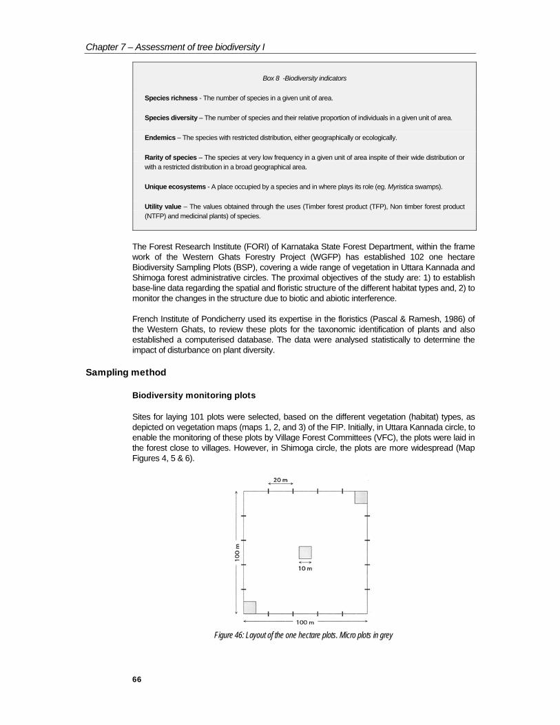
Sites for laying 101 plots were selected, based on the different vegetation (habitat) types, as depicted on vegetation maps (maps 1, 2, and 3) of the FIP. Initially, in Uttara Kannada circle, to enable the monitoring of these plots by Village Forest Committees (VFC), the plots were laid in the forest close to villages. However, in Shimoga circle, the plots are more widespread (Map Figures 4, 5 & 6).
Figure 46: Layout of the one hectare plots. Micro plots in grey

Chapter 7 – Assessment of tree biodiversity I
67
Each plot measures 100 X 100 m (one hectare). At every 20 m along the boundary of the plot, permanent stone posts have been fixed (Figure 46). In the entire plot (macro plot), all the plant individuals equal to or more than 10 cm GBH (girth at breast height, that is at 137 cm from the ground) were tagged (aluminium plates) with serial numbers and botanically identified. Their GBH were measured and heights were estimated. General information on the plot, such as location, bio-climate, slope, aspect, vegetation type, and evidence of disturbance (fire, cut stumps, grazing and trails) were noted on a proforma (Annexe 2). On a whole plot basis parameters like canopy height (m), canopy cover (%) and number of strata were visually estimated.
In order to study the regeneration, 3 (10x10m) micro plots were established in a diagonal axis across the 1 ha plots. In these subplots all the individuals less than 10 cm girth and more than 1 m height were identified and counted. The individuals less than 1 m were enumerated. Canopy cover over each subplot was estimated and also any presence of cut stumps was counted.
For the present study only 96 plots have been considered. The remaining 6 plots are mixed with plantation trees.
Database and Application Development
The Sampling Plot Database was designed as a Relational Database Management System (RDBMS) using MS Access™. The database consists of a complex relational structure with 40 tables and some 42 queries (Figure 47). It consists of a built-in application for data-entry and front-end applications for calculating various statistical indices. The database is shared and kept on a central server. Various third party software packages, namely statistical packages like Statistica™ is connected directly to the database tables or queries through an external Other Database Connectivity (ODBC) connection.
The aim is to have an optimised database with high levels of normalisation to ensure a robust, distributable and compatible data-model that can be used and distributed through front-end tools and third party software packages.
Special care was taken to design the interface for making it compatible and convenient in terms of the existing data and the data-collection methods being followed.
The data can be classified into the following main categories:
• Sample Plots
• Sample Micro-plots
• Trees
• Species
• Physical Environment (Forest Types, Topography)
• Administrative Units
• Qualitative Plant Parameters (Habit, Endemic, Ecology, Phenology)
• Usage (Medicinal, TFP, NTFP)

Chapter 7 – Assessment of tree biodiversity I
68
Plot
Circle Division
ForestType
Terrain
Trees
MicroPlots
SpeciesFamily Medicine
Non-timberforest
product
Timberforest
product
HabitPhenologyEcologyEndemic
Figure 47: A block diagram showing the main relations between the tables of the database.
Report
A sophisticated report was designed for each plot. The report lists out the various parameters, calculated indices and qualitative plant parameters relating to the plot. Graphs for Girth Distribution, Species Individual Curve, Individuals per Species is also plotted dynamically for each plot in the report (Figure 48).
Chapter 7 – Assessment of tree biodiversity I
69
Macros (VBA™)
Macros were built using VBA™ (Visual Basic for Applications) for obtaining certain listings such as proportion of species relating to qualitative plant parameters at the plot and micro-plot levels.
Figure 48: Layout of a sample plot report
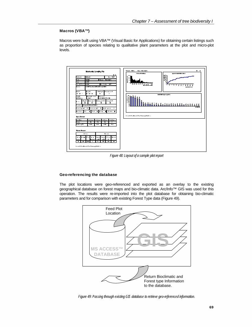
Geo-referencing the database
The plot locations were geo-referenced and exported as an overlay to the existing geographical database on forest maps and bio-climatic data. Arc/Info™ GIS was used for this operation. The results were re-imported into the plot database for obtaining bio-climatic parameters and for comparison with existing Forest Type data (Figure 49).
Feed PlotLocation
GISMS ACCESS™
DATABASE
Return Bioclimatic andForest type Informationto the database.
Figure 49: Passing through existing GIS database to retrieve geo-referenced information.
Chapter 7 – Assessment of tree biodiversity I
70
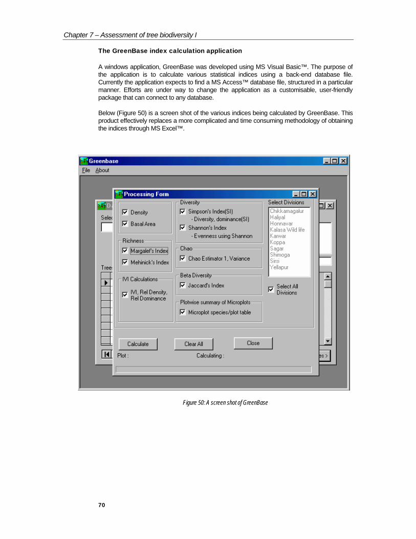
The GreenBase index calculation application
A windows application, GreenBase was developed using MS Visual Basic™. The purpose of the application is to calculate various statistical indices using a back-end database file. Currently the application expects to find a MS Access™ database file, structured in a particular manner. Efforts are under way to change the application as a customisable, user-friendly package that can connect to any database.
Below (Figure 50) is a screen shot of the various indices being calculated by GreenBase. This product effectively replaces a more complicated and time consuming methodology of obtaining the indices through MS Excel™.
Figure 50: A screen shot of GreenBase
Chapter 7 – Assessment of tree biodiversity I
71
Diversity indices
Physical appearance and species composition of the vegetation depend on the magnitude of biotic and abiotic interference. The indices to measure the responses of vegetation to these factors are classified into two categories. They are spatial structure and floristic structure indices. These indices are calculated for each plot (alpha diversity).
Spatial structure
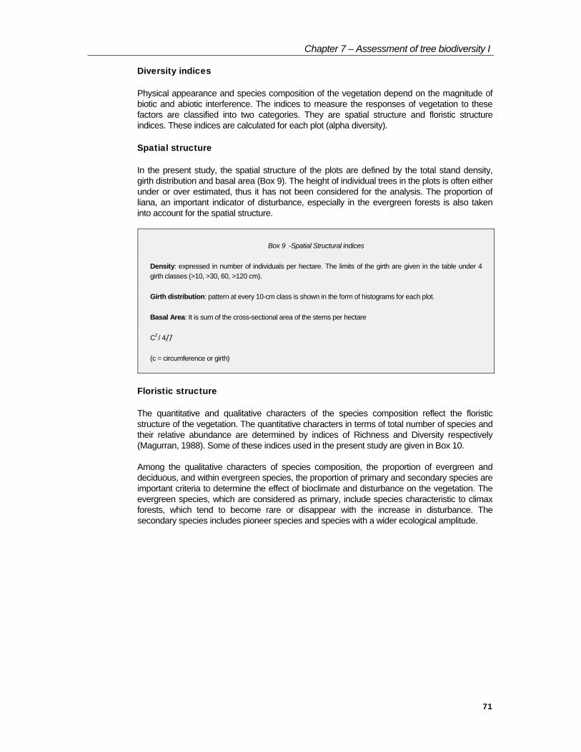
In the present study, the spatial structure of the plots are defined by the total stand density, girth distribution and basal area (Box 9). The height of individual trees in the plots is often either under or over estimated, thus it has not been considered for the analysis. The proportion of liana, an important indicator of disturbance, especially in the evergreen forests is also taken into account for the spatial structure.
Box 9 -Spatial Structural indices
Density: expressed in number of individuals per hectare. The limits of the girth are given in the table under 4 girth classes (>10, >30, 60, >120 cm).
Girth distribution: pattern at every 10-cm class is shown in the form of histograms for each plot.
Basal Area: It is sum of the cross-sectional area of the stems per hectare
C2 / 4∏
(c = circumference or girth)
Floristic structure
The quantitative and qualitative characters of the species composition reflect the floristic structure of the vegetation. The quantitative characters in terms of total number of species and their relative abundance are determined by indices of Richness and Diversity respectively (Magurran, 1988). Some of these indices used in the present study are given in Box 10.
Among the qualitative characters of species composition, the proportion of evergreen and deciduous, and within evergreen species, the proportion of primary and secondary species are important criteria to determine the effect of bioclimate and disturbance on the vegetation. The evergreen species, which are considered as primary, include species characteristic to climax forests, which tend to become rare or disappear with the increase in disturbance. The secondary species includes pioneer species and species with a wider ecological amplitude.

Chapter 7 – Assessment of tree biodiversity I
72
Box 10 – Floristic Structural indices
Species richness
Species-individual curve: cumulative number of species with increase in number of individuals.
Marglef index (Mg): A simple procedure used to estimate the richness by equation DMg = (Sobs – 1)/ ln N
Chao 1 index: It is used to include the role of rarity in estimating the richness. S1 = Sobs + (a2/2b)
Species diversity
Simpson's index: is defined from as probability that two individuals randomly and independently selected belong to the same species. This index has been calculated using the formula:
D ∑ −−
=)1()1(
NNnn ii
The Simpson index can be defined in two ways:
as λ = 1-D, also called dominance index ; it varies between 0 (for a one species community) to 1-1/S (for an even community composed of S species)
as λ’ = 1/D; it varies between 1 (for 1 species community) and S.
Shannon's Index: This index is defined as:
ii ppH ln' ∑−=
(pi = proportional abundance of the i th species)
)/( Nnp ii =
Evenness using Shannon Index:
SHE ln/'=
(H' = Shannon's index)
(Sobs = total number of species observed; ln = logarithm; N = total number of individuals; ni = number of individuals of the ith species; a = the number of observed species that are represented by a single individual; b = the number of observed species represented by two individuals in the sample)
Analyses
The statistical analyses for the macro plots were carried out in two steps: (1) According to global analyses involving all the 96 plots and 400 species (excluding 29 unidentified species, mostly from lianas) (2) Based on major vegetation types.
Chapter 7 – Assessment of tree biodiversity I
73
Global analyses
In order to assess the relationship between climate and vegetation types, and the effect of disturbance on spatial and floristic structure of the vegetation, the following multivariate analyses were conducted using ADE4 software package with an interface for Windows 98 (Thioulouse et al., 1995)
Correspondence analysis (CA) was performed on the data matrix composed of plots and species density to obtain a typology of forests.
Multiple correlation analysis (MCA) was accomplished using the data set between plot and bioclimatic variables (rainfall and length of the dry season) to characterise the main bioclimatic conditions.
To study the link between structural parameters and the typology of vegetation, principal component analysis (PCA) was done on the data matrix composed of spatial and floristic structural variables against plots.
To understand the relationship between bioclimate and vegetation types following methods were adopted.
For each plot, bioclimatic categories such as rainfall (>5000, 2000-5000, 1200-2000, 900-1200 and <900 mm) and length of the dry season (4, 5, 6 and 7 months were determined by superimposing the plots on bioclimatic map (Pascal, 1982). Since there are only two categories, temperature has not been considered.
As the bioclimatic categories are qualitative, coordinates of the factors obtained from the MCA and CA were used as synthetic variables for simple regression analysis to define the link between vegetation types and climate.
Forest type wise analyses
Based on the results of above analyses, which are more or less similar to our field observation, the plots were grouped into physiognomic classes. These groups are further classified under major vegetation types based on ecology and phenology.
In order to understand the significance and relationship of structural and floristic variables vis a vis disturbance gradient, the forest groups are subjected to following statistical analyses.
Analysis of variance (ANOVA) was performed to test the significant differences between forest groups for structural and floristic variables.
Those significant variables obtained for the groups from the above analysis are further subjected to simple correlation analysis to know the relationship between two variables.
Regeneration
For regeneration studies, 3 micro plots in each macro plot were merged as one sample (300 m2). They are classified into similar groups as that of macro plots. In order to understand the effect of disturbance on the regeneration of tree species ANOVA was performed on the data composed of tree saplings.
Chapter 7 – Assessment of tree biodiversity I
74
Buffer analysis
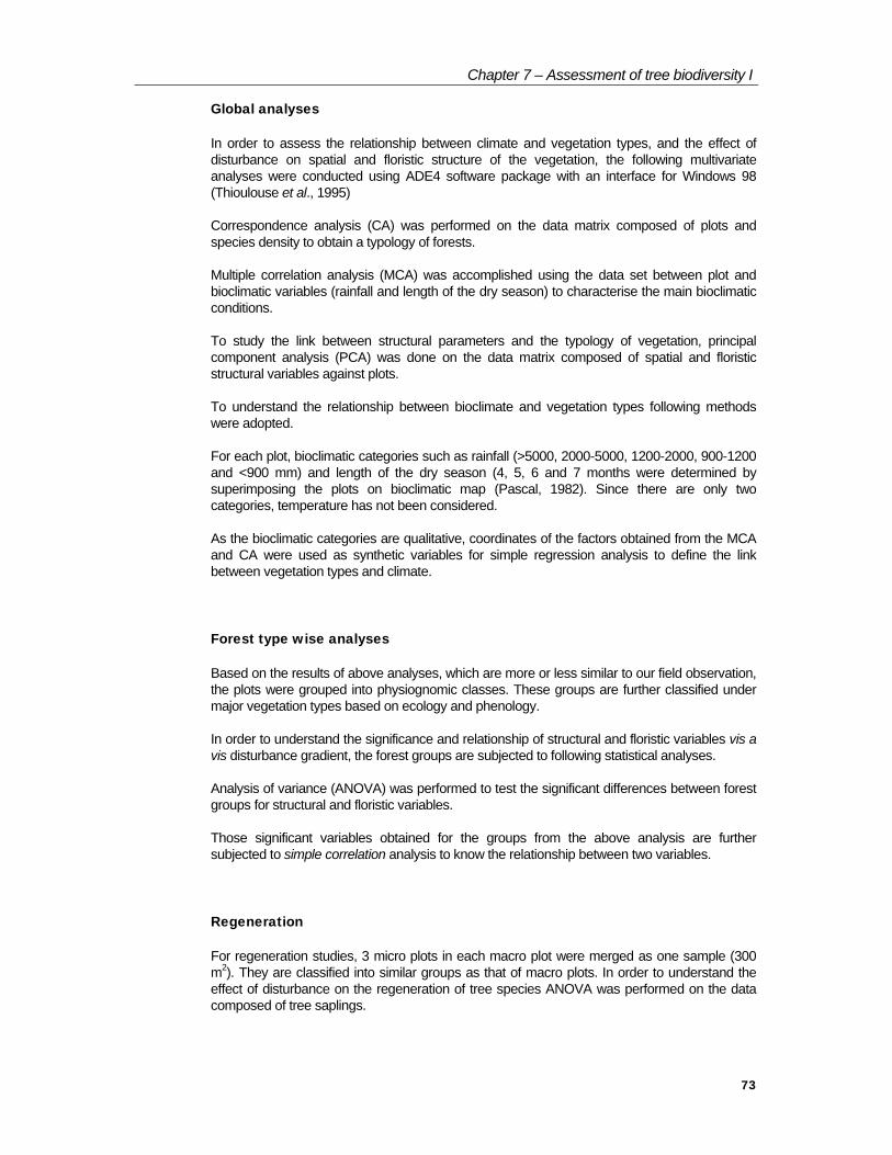
This analysis was done to understand the effect of proximity and proportion of area covered by anthropogenic patches on the physiognomy of the forest sampled. A buffer was created around the BSPs using Arc/Info on the vegetation layer of 1997. The area thus created was clipped from the vegetation layer, and the proportion of total area covered by anthropogenic types was determined for each plot. A buffer and clip was performed for both buffer distances of 500 meters and 1000 meters (Figure 51).
Figure 51: A clip of buffer area around sample plot no. 93.
The physiognomic levels of the forest plots sampled were classified in a similar way as previous analyses. For each physiognomic group mean area (in percentage) of anthropogenic patches were calculated and the results were depicted according to major vegetation types in the form of histograms.
Resource diversity
Resource value of species is also one of the important criteria in the evaluation of biodiversity. Non-sustainable harvesting of some of the species may have repercussion on the their population structure, and eventually on biodiversity. In the present study, attempts have been made to understand the resource value of habitats and the effect of degradation on the population structure of some useful species.
The utility values of the species recorded from the BSPs were determined by consulting several published literatures (Bourdillon, 1908; Caius, 1986; Chandrabose & Nair, 1987; Jain, 1981; Keshava Murthy & Yoganarasimhan, 1990; Rama Rao & Sahib, 1914; Subramanian, 1995; Subramanian, Venkatasubramanian & Nallaswamy, 1987). The values are classified into three categories: timber forest product (TFP), non-timber forest product (NTFP) and medicinal. A number of useful species present in the major types of vegetation have been determined. Population densities of some selected species were compared according to degradation stages.

75
Assessment of tree biodiversity: Part II Observations on biodiversity sampling plots (BSP) and on their species composition
Results
Biodiversity sampling plots
The Karnataka Forest Department (KFD) has three circles in its Western Ghats forestry project jurisdiction. In the first phase of their programme, 101 biodiversity plots have been established in Uttara Kannada (northern part) and Shimoga (central part) circles (Annexe-3). In these circles, plots are represented in 6 divisions in the former circle and 4 divisions in the latter.
Reserved Forests (RF) constitute the basic unit of the protected area (PA) network in the forest administration. Uttara Kannada and Shimoga circles have 368 (some time as blocks) and 175 RFs respectively. Among the BSPs, 57 covers only 33 RFs in total and rest of them are outside the PA net work.
In the map 1, 2 & 3 fiftyfour habitat types have been depicted. FORI initially planned to establish two plots per type. However, the superimposition of the plots on these maps shows that BSPs cover only in 28 types.
In the current study, 96 plots have been considered. The remaining 5 plots lie in plantation areas.
Species composition
Totally 498 taxa are encountered in 96 plots (Annexe-4). Of these, 429 are found in the macro plots. In the micro plots, 345 species of above 1 m height and <10 cm girth, and 240 species of below 1< m height are recorded (Table 7).Table 7: Number of species according to habit encountered in BSPs
Habit Macro plot Micro plot(≥1m h ≤10cm G)
Micro plot(<1 m)
Tree 351 262 165Woody liana 78 41 30Shrub 17 14Herb 8 17Climber 17 14Total 429 345 240
Totally 61,971 individuals from macro plots and 16,755 from micro plots covering 498 species under 302 genera and 90 families have been recorded. Among the families Rubiaceae,
Chapter
8

Chapter 8 – Assessment of tree biodiversity II
76
Euphorbiaceae, Lauraceae and Moraceae constitute 21% of the total number of species. The first two families have contributed more genera as well as species number (Table 8). Considering the total tree individuals in the macro plot, 60% of them come from 29 species only (Table 9). Within these species Terminalia paniculata (3,811) counted highest number of individuals followed by Xylia xylocarpa (3,498), Terminalia tomentosa (1,653), Tabernamontana heyneana (1,387) from Secondary and primary moist deciduous; Poeciloneuron indicum (2,220), Hopea ponga (1,873) and Knema attenuata (1,762) from Wet evergreen; Aporosa lindleyana (1,776), Holigarna arnottiana (1,341), Olea dioica (2,366), Ixora brachiata (1,396), and Dimocarpus longan (1187) from disturbed evergreen and semi evergreen forests; Anogeissus latifolia (938) from dry deciduous forest forests. The number of species and their individual contribution to total frequency for all the macro plots are shown under seven classes (Figure 52).
Number of species and individual contribution
0
50
100
150
200
250
300
1-5
0
50-1
00
100-
300
300-
500
500-
1000
1000
-200
0
>200
0
Individuals
Spe
cies
Figure 52: Number of species contributing to frequency classes
Further, these species are classified based on phenological and ecological characteristics. Evergreen species are higher in number (78%) compared to deciduous species (22%). Within evergreen, primary and secondary species represent 52 and 48% respectively (Figure 53).
192
175
102
Primary evergreen
Secondary evergreen
Deciduous
Figure 53: Repartition of species based on phenological and ecological characteristics

Chapter 8 – Assessment of tree biodiversity II
77
Table 8: List of families with number of genera and species encountered in the macro plots Family Genus Species Family Genus Species
Rubiaceae 19 32 Araliaceae 1 2Euphorbiaceae 23 30 Capparidaceae 1 2Lauraceae 8 23 Simarubaceae 1 2Moraceae 4 21 Convolvulaceae 2 2Fabaceae (Mimosoideae) 7 18 Hippocrateaceae 2 2Meliaceae 14 18 Liliaceae 2 2Ebenaceae 1 15 Olacaceae 2 2Annonaceae 12 15 Theaceae 2 2Rutaceae 12 15 Urticaceae 2 2Fabaceae (Caesalpinioideae) 8 14 Zingiberaceae 2 2Fabaceae (Faboideae) 10 13 Adiantaceae 1 1Myrtaceae 3 11 Alangiaceae 1 1Clusiaceae 5 10 Amaryllidaceae 1 1Flacourtiaceae 5 10 Ancistrocladaceae 1 1Anacardiaceae 7 10 Asclepiadaceae 1 1Apocynaceae 7 9 Bombacaceae 1 1Celastraceae 6 8 Cornaceae 1 1Verbenaceae 7 8 Datiscaceae 1 1Rhamnaceae 3 7 Dichapetalaceae 1 1Combretaceae 4 7 Dilleniaceae 1 1Sapotaceae 6 7 Elaeagnaceae 1 1Sapindaceae 7 7 Gnetaceae 1 1Melastomataceae 2 6 Lamiaceae 1 1Sterculiaceae 3 6 Lecythidaceae 1 1Dipterocarpaceae 4 6 Leeaceae 1 1Symplocaceae 1 5 Magnoliaceae 1 1Tiliaceae 1 5 Malpighiaceae 1 1Boraginaceae 3 5 Malvaceae 1 1Vitaceae 3 5 Ochnaceae 1 1Bignoniaceae 4 5 Osmundacea 1 1Icacinaceae 4 5 Oxalidaceae 1 1Myrsinaceae 4 5 Pandanaceae 1 1Oleaceae 4 5 Pittosporaceae 1 1Ulmaceae 4 5 Poaceae 1 1Acanthaceae 5 5 Polgonaceae 1 1Arecaceae 5 5 Proteaceae 1 1Elaeocarpaceae 1 4 Pteridaceae 1 1Loganiaceae 2 4 Ranunculaceae 1 1Lythraceae 1 3 Rhizophoraceae 1 1Connaraceae 2 3 Rosaceae 1 1Myristicaceae 2 3 Selaginelaceae 1 1Piperaceae 2 3 Smilacaceae 1 1Araceae 3 3 Solanaceae 1 1Asteraceae 3 3 Staphylaceae 1 1Burseraceae 3 3 Thymelaeaceae 1 1Menispermaceae 3 3 Unidentified 29Santalaceae 3 3 Total 302 498

Chapter 8 – Assessment of tree biodiversity II
78
Table 9: List of species, with over 500 individuals represented in macro plot
SpeciesNumber
ofindividuals
Terminalia paniculata 3811Xylia xylocarpa 3498Olea dioica 2366Poeciloneuron indicum 2220Hopea ponga 1873Aporosa lindleyana 1776Knema attenuata 1762Terminalia tomentosa 1653Ixora brachiata 1396Tabernaemontana heyneana 1387Holigarna arnottiana 1341Catunaregam dumetorum 1209Dimocarpus longan 1187Lagerstroemia microcarpa 999Tectona grandis 996Anogeissus latifolia 938Calycopteris floribunda 905Memecylon umbellatum 890Flacourtia montana 798Symplocos racemosa 778Aglaia barberi 713Careya arborea 651Holigarna grahamii 630Callicarpa tomentosa 610Chionanthus malabaricus 583Syzygium cumini 570Xantolis tomentosa 568Garcinia morella 519Diospyros candolleana 501Total 37128
Vegetation types and its relationship with bioclimate
Correspondence analysis (CA) to determine the typology of the forests
Matrix of 96 plots and density of 400 species (excluding 29 unidentified) were subjected to CA. The first three factors F1, F2 and F3 accounts for 8, 7 and 5% of the total inertia respectively. F1 is determined by the extremely wet zone species like Poeciloneuron indicum (absolute contribution 14%) on the one hand and on the other by moist zone species like Terminalia paniculata (8%) and Xylia xylocarpa (9%). F2 is mostly determined by the wet zone species, and again maximum absolute contribution comes from Poeciloneuron indicum (22%). F3 axis determined by the dry zone species like Anogeissus latifolia (30%), Chloroxylon switenia (12%), Albizia amara (7%) and Acacia catechu (7%) on one side, and on the other Xylia xylocarpa (15%), a dominant species in the intermediate zone between the moist and dry.

Chapter 8 – Assessment of tree biodiversity II
79
With the ordination of F1 and F3, which gives a better dispersion of the plots (Figure 54), seven distinct groups of plots have been identified. These groups are derived from the combination of certain dominant species characteristic to particular vegetation types (Table 10). The groups A, B and C composed of plots from wet evergreen, semi evergreen and moist deciduous forest are aligned along F1 and group D having dry deciduous plots are arranged along F3.
1 2
3
4
56
78
910
11 12 131415
16
17
18
20
21
2223
24
25
2627
28
29 30
31 3334
35
36
3741
42
43
44
45
4647
48 49
5051
52 53
5455
56
57
58
59
60
61
62
63
646566 67 68
69
70
71
72
737475
76
78
7980
82
83
84
8586
87
88
89
909192
9394
95
96
97
98
99
100
101
102
104
Plots
F1
1
478 911 14
19
23
2429
31
3540
43 48
60 65
67 6970
75 78
85
9095
96
102
103106108109
111
112113 115
118119120
123126128
129
133134137141142
146147148150
154155
158160162 164
168
170
171
172
180
182187189
190
194195197
204205212
214217219
221
226 235 240242
247
254 262266
269271274 276279
281
282285289290
291292
299
301 302
304
306311
313318323
325
331332
336338
340
341
347348
349352353365369371
372373378381382387
388
393
394396
397399401
402403
404
405407 408
409410
411
412
413 414415
417418420
426
429439442
449452
453454455
457
470477
480
484
486487
491500
505508516
522532
540
544555560
561563
565566
568
570
571572
573
577578580581585587
592
593596598600601
603608610 613
615
617621
628
630631
634635
639
645
646
647
649
650
651653655
656657
658
660
661 662
663664
665
666667 668
669
671
672
673674
675676677
678
679
681682
684
685
686
688689690
691
692
693
694
696
697698
699
700 702703 704705
708
709710
711
712
714
716
717718
719 720721 723
725
726
727
728 730 731732
733
734
735736
737
738
739740
742
743
744
745
747748
749750
751
754
755
756
757
758
759
760762764
767
774776 778782
783787
788
802
813
817
819
821827833837
839840
841
843
855857
858860
864867
868871
872873875
876
878879880
881884
885
895
899 900
901902
903
904
905
906
907
909910
911
913916
917920
963966 967
971 972973974975980985
987988989
992993995 996
999
1002100310041011
10131014
10171018
1019
1021
1046 10511055105610571059
1060
Species F3
F1
F3
A1
A2
D1
C2
BC1
D2
Figure 54: Correspondence analysis for 96 plots and 400 species on factor 1 and 3 (for species code see annex 4).
Chapter 8 – Assessment of tree biodiversity II
80
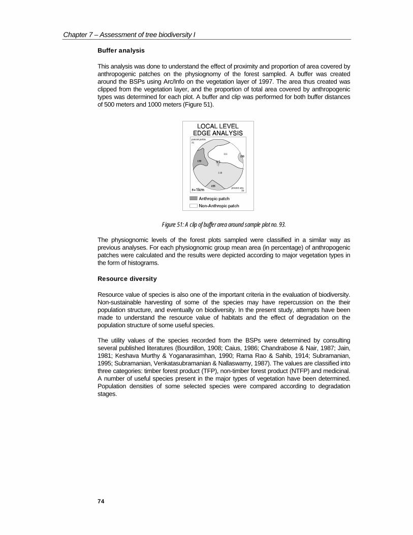
Table 10: Major forest types and dominant species belongs to groups obtained from factorial analysis of correspondence. Species with absolute contribution more than 7% to first three factors are highlighted.
Groups Forest types Dominant species
A1Poeciloneuron indicum (F1, F2)Cleistanthus malabaricus (F2)Dipterocarpus indicus
A2
Wet evergreenclimax and non-climax forests
Hopea pongaKnema attenuataHoligarna arnottianaOlea dioicaDimocarpus longanMemecylon umbellatum
B Semi evergreenand ‘Kan’ forests
Olea dioicaAporosa lindleyanaHoligarna arnottianaIxora brachiataFlacourtia montanaChionanthus malabaricus
C1Secondary moistdeciduous andPrimary moistdeciduous forests
Terminalia paniculata (F1)Terminalia tomentosaLagerstroemia microcarpaTectona grandis
C2Primary moistdeciduous forests
Xylia xylocarpa (F1, F3)Terminalia tomentosa
D1 Dry deciduous(transition)
Anogeissus latifoliaTerminalia paniculataTerminalia tomentosaTectona grandis
D2 Dry deciduousAnogeissus latifolia (F3)Chloroxylon swietenia (F3)Albizia amara (F3)Acacia catechu (F3)
Group A1 represents climax evergreen forests (as shown on the maps 1 and 2) and is determined by the gregarious presence of Poeciloneuron indicum. Plots (ID) 65, 66 and 67, which are at medium elevation (>900 m) near the Kudremukh area are distinct within the group, due to the co-dominance of Cleistanthus malabaricus with Poeciloneuron. Whereas Dipterocarpus indicus is a characteristic canopy species of low elevation wet evergreen forests distinctly associated with Poeciloneuron in plot ID 75.
Group A2 represents both climax and non-climax disturbed wet evergreen forests. Even though Hopea ponga and Knema attenuata are understorey primary species, they tend to become dominant in areas at early stages of disturbance. Dimocarpus longan, Olea dioica, Holigarna arnottiana are very common in secondary forests. Memecylon umbellatum is abundant in the climax forests (plot ID 89, 90, 91), north of the Kali river valley.
Group C1 is composed of plots from primary and secondary moist deciduous forests. Terminalia paniculata, Terminalia tomentosa, Lagerstroemia microcarpa and Tectona grandis are the most common species in these forests. Group C2 plots are although of primary moist deciduous forests, they are dominated by Xylia xylocarpa.
Group D plots in general are abundant with Anogeissus latifolia. However, D1 group, which is closer to C1 also have Terminalia spp. and Tectona grandis as common species. Anogeissus latifolia, Chloroxylon switenia, Albizia amara and Acacia catechu, which are typically of dry deciduous forests, dominate the group D2.
Chapter 8 – Assessment of tree biodiversity II
81
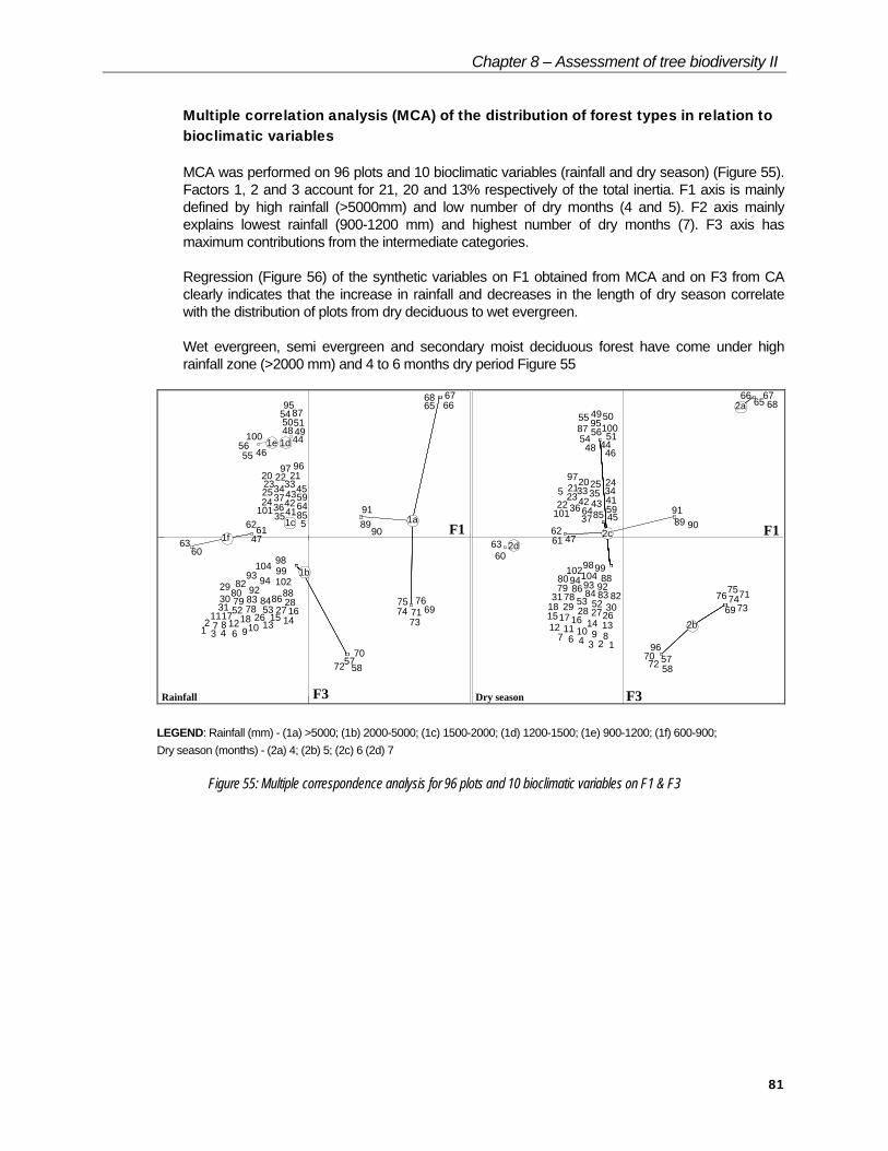
Multiple correlation analysis (MCA) of the distribution of forest types in relation to bioclimatic variables
MCA was performed on 96 plots and 10 bioclimatic variables (rainfall and dry season) (Figure 55). Factors 1, 2 and 3 account for 21, 20 and 13% respectively of the total inertia. F1 axis is mainly defined by high rainfall (>5000mm) and low number of dry months (4 and 5). F2 axis mainly explains lowest rainfall (900-1200 mm) and highest number of dry months (7). F3 axis has maximum contributions from the intermediate categories.
Regression (Figure 56) of the synthetic variables on F1 obtained from MCA and on F3 from CA clearly indicates that the increase in rainfall and decreases in the length of dry season correlate with the distribution of plots from dry deciduous to wet evergreen.
Wet evergreen, semi evergreen and secondary moist deciduous forest have come under high rainfall zone (>2000 mm) and 4 to 6 months dry period Figure 55
65 666768
697173
7475 76
8991
1a
12
3 4 67 8
91011
12 13 1415 1617 18 2627
28293031 52 53
575870
72
78798082
83 848688
90
9293 94
9697
9899102
104 1b
5
20 212223
2425
3334
353637
41424345
596485101
1c
4448 49505154 8795
1d4655
56100 1e
4760
6162
63 1f
Rainfall
6566 6768
97
2a
5758
69
70
71
72
73747576
96
101
2b
1234
5
67 89101112 131415 161718
2021
2223
2425
26272829 3031
33 343536
37
4142 43
44
45
46
47
48
4950
51
5253
54
5556
59
6162
64
787980
828384
85
86
87
88
89 9091
929394
95
9899
100
102104
2c
6063 2d
Dry season
F1
F3 F3
F1
LEGEND: Rainfall (mm) - (1a) >5000; (1b) 2000-5000; (1c) 1500-2000; (1d) 1200-1500; (1e) 900-1200; (1f) 600-900; Dry season (months) - (2a) 4; (2b) 5; (2c) 6 (2d) 7
Figure 55: Multiple correspondence analysis for 96 plots and 10 bioclimatic variables on F1 & F3

Chapter 8 – Assessment of tree biodiversity II
82
y = -0.346x2 + 2.750x + 0.206R2 = 0.84
0
1
2
3
4
5
6
7
0 1 2 3 4 5 6F1 (bioclimate)
F3 (p
lots
)
Figure 56: Regression analysis of synthetic variables obtained from MCA (F1, bioclimate) and CA (F3, plots)
Poeciloneuron dominates all the plots in A1 group (obtained from FCA). In A2, plots dominated by Memecylon umbellatum and some disturbed plots (71, 76 and 69), which are in the potential distribution area of Poeciloneuron corresponds to >5000 mm category of rainfall. However, when the length of the dry season is considered, the same plots, come under 3 categories of dry season. Plots in Kudremukh (southern most plots among BSPs) at medium elevation (>900 m) experience 4 months dry period, whereas Memecylon forests (northern most plots) encounter 6 to 7 months. Plots (73, 74, 75), particularly with Poeciloneuron and Dipterocarpus indicus together at lower elevations (600 – 700 m), have 5 months dry period. The rest of the plots in evergreen, semi evergreen and secondary moist deciduous are found in rainfall zone between 2000 to 5000 mm and 6 months dry period.
‘Kan’ evergreen forests (plots 5, 36, 37 and 42), an edaphic facies in Soraba region are found between 1500 to 2000 mm rainfall and 6 months dry period, similar to primary moist deciduous forests.
Primary moist deciduous forests come under 1200 to 2000 mm rainfall and 6 months dry period and dry deciduous forests experience 600 to1200 mm rainfall and 6 to 7 months dry period.
Vegetation types in relation to spatial and floristic parameters
Ninety-six plots were ordinated with 11 spatial and floristic variables (as given in Figure 57) in a principal component analysis (PCA).
The F1 and F2 account for 29 and 17% of the total variations respectively. The combination of these two factors Figure 57 indicates that the density of evergreen species is the most influencing variable. It ordinates the plots along the F1, in the order of phenological groups from evergreen, semi evergreen to deciduous.
Chapter 8 – Assessment of tree biodiversity II
83
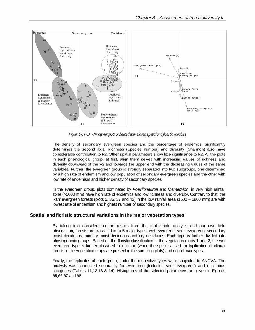
Figure 57: PCA - Ninety-six plots ordinated with eleven spatial and floristic variables
The density of secondary evergreen species and the percentage of endemics, significantly determines the second axis. Richness (Species number) and diversity (Shannon) also have considerable contribution to F2. Other spatial parameters show little significance to F2. All the plots in each phenological group, at first, align them selves with increasing values of richness and diversity downward of the F2 and towards the upper end with the decreasing values of the same variables. Further, the evergreen group is strongly separated into two subgroups, one determined by a high rate of endemism and low population of secondary evergreen species and the other with low rate of endemism and higher density of secondary species.
In the evergreen group, plots dominated by Poeciloneuron and Memecylon, in very high rainfall zone (>5000 mm) have high rate of endemics and low richness and diversity. Contrary to that, the ‘kan’ evergreen forests (plots 5, 36, 37 and 42) in the low rainfall area (1500 – 1800 mm) are with lowest rate of endemism and highest number of secondary species.
Spatial and floristic structural variations in the major vegetation types
By taking into consideration the results from the multivariate analysis and our own field observation, forests are classified in to 5 major types: wet evergreen, semi evergreen, secondary moist deciduous, primary moist deciduous and dry deciduous. Each type is further divided into physiognomic groups. Based on the floristic classification in the vegetation maps 1 and 2, the wet evergreen type is further classified into climax (when the species used for typification of climax forests in the vegetation maps are present in the sampling plots) and non-climax types.
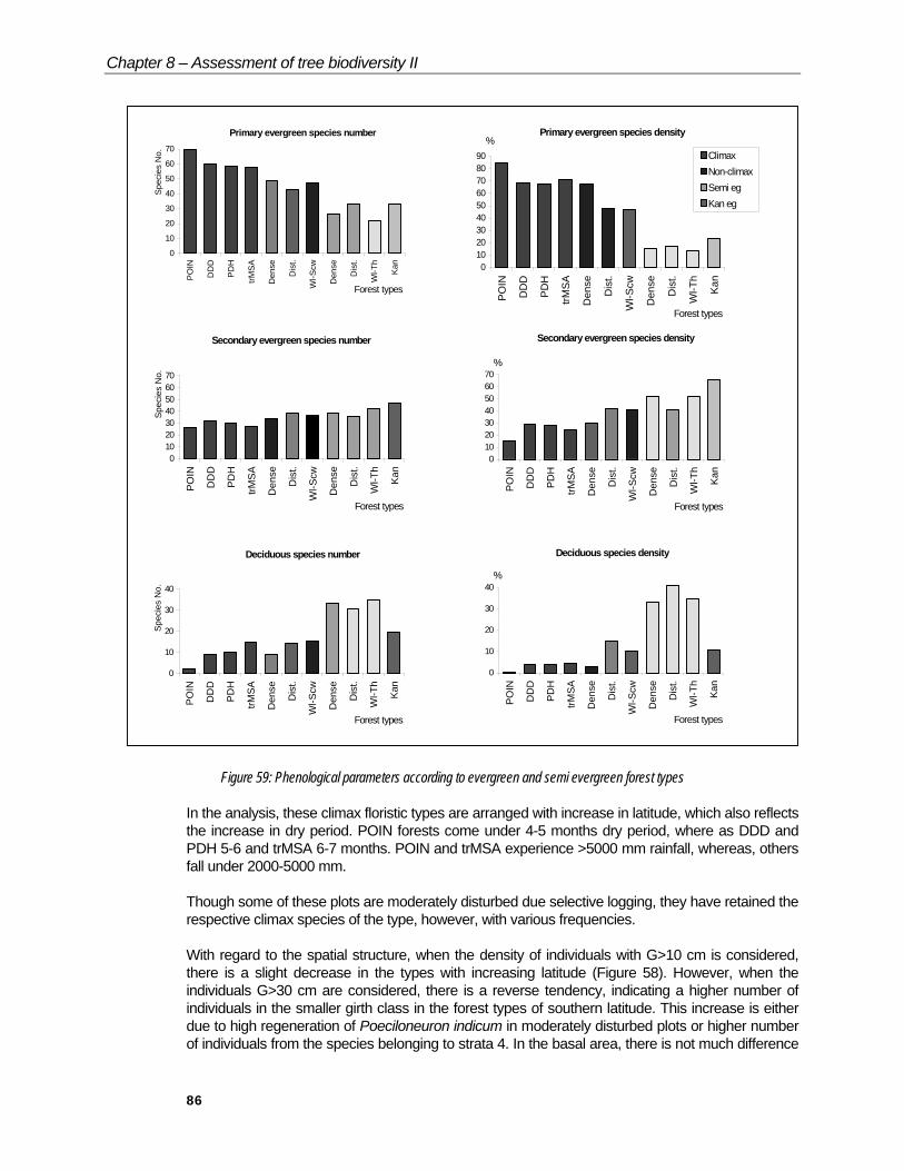
Finally, the replicates of each group, under the respective types were subjected to ANOVA. The analysis was conducted separately for evergreen (including semi evergreen) and deciduous categories (Tables 11,12,13 & 14). Histograms of the selected parameters are given in Figures 65,66,67 and 68.

Chapter 8 – Assessment of tree biodiversity II
84
Evergreen and semi evergreen category
Wet evergreen climax forests
Thirteen BSPs represent 4 floristic climax types: Poecilineuron indicum dominated type (POIN), Dipterocarpus indicus – Diospyros candolleana – Diospyros oocarpa type (DDD), Persea macrantha – Diospyros spp. – Holigarna spp. type (PDH), transition Memecylon umbellatum – syzygium cumini – Actinodaphne angustifolia type (trMSA). In fact, the first type also includes the low elevation dipterocarp forests described in map 2, however, in association with Poeciloneuron indicum. As the samplings in these forests are uneven, they are grouped together as Poecilineuron indicum dominated type.
Table 11: Mean variation (ANOVA) of spatial parameters in the evergreen and semi evergreen forest types. Spatial structure
Density Basal area (m2)Forest types
G>10cm G>30cm G>60cm G>120cm G>10cm G>30cm G>60cm G>120cm
POIN 1230.8 542.5 189.25 59.75 37 34.75 29.75 22.75DDD 1192.7 640.67 274.67 59.67 32 30 24.67 13PDH 1159.7 631.67 293.33 61.67 35.67 34.67 29.33 16.67
Climax
trMSA 1047.3 659.67 293.33 47.33 31.67 30 24.67 10.67Dense 1254 540 244.4 78.2 42.2 40 36 26.4Dist 738.83 375.67 200.67 62.5 29.83 28.67 25.83 17.83Non climax
Wl-Scw 629.33 358.67 182.67 66.33 31 30.33 28 21.33Dense 1117.5 498.25 259.5 60.25 31.25 29.5 26 13.75Dist 575.75 377 244.25 75.5 29.25 29 27 15.75Semi
evergreenWl-Scw 488.75 217.75 124.75 30.5 15 14.5 13 7.25
Kan 849.75 249 144.75 83.5 33.25 31.25 30.25 26.5CD at 5% 235.75 120.25 56.92 28.75 13.25 13.10 12.10 6.3
(Dist = disturbed; Wl = woodland; Scw = scrub woodland) Table 12: Mean variation (ANOVA) of floristic structural parameters in the evergreen and semi evergreen forest types.
Floristic structureForest types S Mg Chao1 End 1/D 1 - D H' E Psp(s) Psp(D) Ssp(s) Ssp(D) Egsp(s) Egsp(D) Desp(s) Desp(D)
POIN 56.25 7.76 88.34 49.75 7.32 0.83 2.52 0.62 69.75 84.75 26 14.75 98 99.75 2 0.25
DDD 67 9.32 90 43.67 15.16 0.93 3.23 0.77 60 68.33 31.67 28.67 90.67 96.33 9.33 3.67
PDH 74.33 10.39 87.31 38.67 13.85 0.93 3.23 0.75 58.67 68 30 28.33 89.67 96.33 10.33 3.67Climax
trMSA 47 6.61 55.03 34.67 8.3 0.86 2.6 0.67 58 71.33 27.33 24 85 95.67 15 4.33
Dense 77 10.69 96.76 37 14.05 0.9 3.14 0.73 48.6 67.6 33.4 29.6 90.8 97.2 8.8 2.8
Dist 69.83 10.44 100.57 32.67 14.31 0.93 3.25 0.77 43 48.17 38 42 86.67 89.33 14.33 14.83
Nonclimax
Wl-Scw 70.33 10.8 95.23 27.67 13.18 0.92 3.22 0.76 47.33 46.67 36.33 41.33 84 89.67 15.33 10.33
Dense 66.5 9.33 86.71 22.25 12.97 0.92 3.11 0.74 26.5 15 38.75 51.5 66.5 66.75 33.5 33.25
Dist 58.25 9.04 76.28 20 17.34 0.94 3.22 0.79 33 17.5 35.5 41 69.5 59.25 30.5 40.75
Semievergreen
Wl-Scw 59 9.38 87.33 17.5 19.4 0.94 3.3 0.82 22.25 13.5 42.25 51.75 65 65.25 35 34.75
Kan 68.75 10.06 89.59 23.5 18.08 0.95 3.33 0.79 33.25 23.5 47 66 80.5 89.25 19.5 10.75
CD at 5% 11.1 2.01 12.24 2.4 3.37 0.02 0.10 0.03 4.15 2.4 5.65 12.58 2.9 5.81 6.5 10.3

Chapter 8 – Assessment of tree biodiversity II
85
Density (G>10 cm)
0150300450600750900
105012001350
PO
IN
DD
D
PDH
trMS
A
Den
se
Dis
t.
Wl-S
cw
Den
se
Dis
t.
Wl-T
h
Kan
Forest types
Indi
vidu
als
(No.
)Density (G>30 cm)
0
150
300
450
600
750
PO
IN
DD
D
PDH
trMS
A
Den
se
Dis
t.
Wl-S
cw
Den
se
Dis
t.
Wl-T
h
Kan
Forest types
Indi
vidu
als
(No.
)
Climax
Non-climax
Semi eg
Kan eg
Basal area (G>10 cm)
05
1015202530354045
PO
IN
DD
D
PD
H
trMS
A
Den
se
Dis
t.
Wl-S
cw
Den
se
Dis
t.
Wl-T
h
Kan
Forest types
m2 Basal area (G>30 cm)
05
1015202530354045
POIN
DD
D
PDH
trMS
A
Den
se
Dis
t.
Wl-S
cw
Den
se
Dis
t.
Wl-T
h
Kan
Forest types
m2
Richness
0
10
20
30
40
50
60
70
80
POIN
DD
D
PDH
trMS
A
Den
se
Dis
t.
Wl-S
cw
Den
se
Dis
t.
Wl-T
h
Kan
Forest types
Spe
cies
No.
(S)
Richness
0
2
4
6
8
10
12
PO
IN
DD
D
PDH
trMS
A
Den
se
Dis
t.
Wl-S
cw
Den
se
Dis
t.
Wl-T
h
Kan
Forest types
Mar
gale
f (M
g)
Diversity
0
0.5
1
1.5
2
2.5
3
3.5
PO
IN
DD
D
PDH
trMS
A
Den
se
Dis
t.
Wl-S
cw
Den
se
Dis
t.
Wl-T
h
Kan
Forest types
Sha
non
(H') Endemic
05
101520253035404550
POIN
DD
D
PDH
trMS
A
Den
se
Dis
t.
Wl-S
cw
Den
se
Dis
t.
Wl-T
h
Kan
Forest types
%
Figure 58: Mean variations in spatial and floristic structural parameters according to evergreen and semi evergreen forest types (POIN = Poiciloneuron indicum dominated types; DDD = Dipterocarpus indicus-Diospyros candolleana- D.oocarpa type; PDH = Persea macrantha-Diospyros spp.-Holigarna spp. type; trMSA = Transition Memecylon umbellatum-Syzygium cumini-Actinodaphne angustifolia type; Dist. = Disturbed; Wl = Woodland; Scw = Scrub woodland; Th = Thicket)
Chapter 8 – Assessment of tree biodiversity II
86
Primary evergreen species number
0
10
20
30
40
50
60
70
PO
IN
DD
D
PD
H
trMS
A
Den
se
Dis
t.
Wl-S
cw
Den
se
Dis
t.
Wl-T
h
Kan
Forest types
Spe
cies
No.
Primary evergreen species density
0102030405060708090
PO
IN
DD
D
PD
H
trMS
A
Den
se
Dis
t.
Wl-S
cw
Den
se
Dis
t.
Wl-T
h
Kan
Forest types
%ClimaxNon-climaxSemi egKan eg
Secondary evergreen species number
010203040506070
PO
IN
DD
D
PDH
trMS
A
Den
se
Dis
t.
Wl-S
cw
Den
se
Dis
t.
Wl-T
h
Kan
Forest types
Spe
cies
No.
Secondary evergreen species density
010203040506070
PO
IN
DD
D
PD
H
trMS
A
Den
se
Dis
t.
Wl-S
cw
Den
se
Dis
t.
Wl-T
h
Kan
Forest types
%
Deciduous species number
0
10
20
30
40
PO
IN
DD
D
PD
H
trMS
A
Den
se
Dis
t.
Wl-S
cw
Den
se
Dis
t.
Wl-T
h
Kan
Forest types
Spe
cies
No.
Deciduous species density
0
10
20
30
40
PO
IN
DD
D
PDH
trMS
A
Den
se
Dis
t.
Wl-S
cw
Den
se
Dis
t.
Wl-T
h
Kan
Forest types
%
Figure 59: Phenological parameters according to evergreen and semi evergreen forest types
In the analysis, these climax floristic types are arranged with increase in latitude, which also reflects the increase in dry period. POIN forests come under 4-5 months dry period, where as DDD and PDH 5-6 and trMSA 6-7 months. POIN and trMSA experience >5000 mm rainfall, whereas, others fall under 2000-5000 mm.
Though some of these plots are moderately disturbed due selective logging, they have retained the respective climax species of the type, however, with various frequencies.
With regard to the spatial structure, when the density of individuals with G>10 cm is considered, there is a slight decrease in the types with increasing latitude (Figure 58). However, when the individuals G>30 cm are considered, there is a reverse tendency, indicating a higher number of individuals in the smaller girth class in the forest types of southern latitude. This increase is either due to high regeneration of Poeciloneuron indicum in moderately disturbed plots or higher number of individuals from the species belonging to strata 4. In the basal area, there is not much difference

Chapter 8 – Assessment of tree biodiversity II
87
between G>10 cm and G>30 cm classes of individuals. DDD and trMSA show relatively less (G>10 = 32 m2) compare to other two (36 – 37 m2) climax types.
In the floristic structure, the species richness (S and Mg) and diversity (Shannon) are relatively low in Poeciloneuron and Memecylon (trMSA) dominated forests compared to DDD and PDH.
When the percentage of endemics are considered, there is a gradual decline in the rate, from 50% to 35% with increase in latitude, which is attributed to increase in length of the dry season from 4 to 6 months.
Among evergreen tree species, primary ones vary from 58 to 60% between DDD, PDH and trMSA type. However, it accounts for 70% in POIN forests. Secondary evergreen species have variations between 26 to 36%. Deciduous species show increase from 2 (POIN) to 15% (trMSA) which may be linked to an increase in dry period (Figure 59).
Non-climax evergreen forests
These forests, also under >2000 mm rainfall zone, are moderately to heavily disturbed; consequently, the species which are typified as climax, are either absent or rarely present. Based on the degree of disturbance, four physiognomic stages (dense, disturbed and wooldland to scrub- woodland) have been identified (Figures 58 & 59).
The forests which are considered as dense have more than 1000 individuals and the density shows a drastic decline to 740 in disturbed forests, and further to 640 in woodland to scrub woodland stages.
The dense forests are similar to climax forests in the total density (1254). However, when the individuals of girth above 30 cm (G>30 cm) are considered, they are fewer (540) than in climax forests. This indicates that more than half the total number of individuals comes from lower girth class. The basal area in the dense forests is much higher (42 m2) compared to all other forest types. Due to the presence of some big trees in the disturbed and woodland to scrub woodland, the basal area (around 30 m2) is nearly similar to climax type and dense or disturbed of semi evergreen type.
Among the floristic structural parameters, species richness shows relatively less variations (70-77 species) between the dense, disturbed and woodland to scrub woodland formations. The diversity value (H’) varies from 3.03 – 3.25. The percentage of endemic species decreases with the increase in disturbance. In all the groups, the number of primary evergreen species varies between 42 and 48% and its density steeply decreases (67 to 35 %) with the increase in degradation. Although the number of secondary evergreen species is less (36 – 39%), its overall density is higher (49-52%) than that of primary species. Numbers of deciduous species also show an increase with degradation. However, its density in dense forest is as low (5%) as climax forest.
Semi evergreen forests
In the dense semi evergreen forests, total density is more than 1100 individuals and in other groups (disturbed to scrub woodland – thickets) it is nearly half of this or less. The basal area in dense and disturbed groups varies between 29 and 31 m2 and in others it accounts for only 15m2 (Figure 58).
Richness (S 58-66) and diversity (H’ 3.3-3.22) in all the physiognomic stages, vary little although endemics show a gradual decline from 22 to 17%.
Chapter 8 – Assessment of tree biodiversity II
88
Predictably in semievergreen forests, evergreen species accounts for 65 to 66% (density 59-67%) and deciduous species represent 30 to 35 % (density 59-67%) of the total number of species. Among the evergreen species, both the number and density, of primary species are less than 33% and secondary species are more than 35% (Figure 59).
‘Kan’ evergreen forests
‘Kans’ are the patches of remnant evergreen forests in the midst of moist deciduous forest where the rainfall is less than 1800 mm. In spite of the constraint in rainfall, ‘Kan’ forests are to a certain extent structurally and floristically, similar to wet evergreen forests. Four plots, which were studied under this type, are moderately disturbed.
Contrasting difference between total density (850) and density (249) of big trees (G>10 cm) indicates the high concentration of individuals at the lower strata. Basal area (33 m2) is nearly equal to dense and disturbed groups of other evergreen and semi evergreen types. Richness (68 species) and diversity (H’ 3.33) is nearly similar to other types. Number of endemics (23%) is equal to dense semi evergreen and less than all the physiognomic groups in other types (Figures 58 & 59).
In the richness and density of evergreen species, ‘Kan’ forests are equal to wet evergreen types. However, within the evergreen, primary species are fewer and secondaries are more numerous compared to wet evergreen types.
Deciduous category
This category is represented by 3 main types: secondary moist deciduous, primary moist deciduous and dry deciduous.
Secondary moist deciduous forests
The deciduous forests in the >2000 mm rainfall zone are considered as secondary, because they are derived from the gradual degradation of wet evergreen forest. Eventhough, the floristic composition among big trees is similar to the primary moist deciduous forests, the undergrowth is well represented by evergreen species, whose density varies between 8-23% and also have 9-15% endemics (Figures 60 & 61).
The total stand density in dense forest is 790. It declines sharply (312) in disturbed woodland stage. However, shows an increase (415-547) with increasing in degradation. And in extreme open conditions like open thickets, density become very low (160)(Figure 60).
In spite of a low density in woodland, when compared to dense forest, its basal area is high (27 m2). In others groups, basal area decreases (15-8 m2) with the increase in degradation.
Chapter 8 – Assessment of tree biodiversity II
89
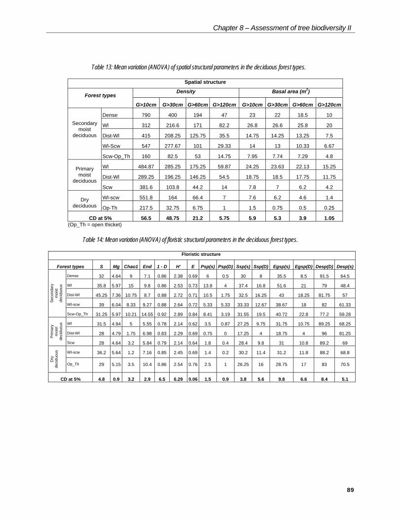
Table 13: Mean variation (ANOVA) of spatial structural parameters in the deciduous forest types.
Spatial structure
Density Basal area (m2)Forest types
G>10cm G>30cm G>60cm G>120cm G>10cm G>30cm G>60cm G>120cm
Dense 790 400 194 47 23 22 18.5 10
Wl 312 216.6 171 82.2 26.8 26.6 25.8 20
Dist-Wl 415 208.25 125.75 35.5 14.75 14.25 13.25 7.5
Wl-Scw 547 277.67 101 29.33 14 13 10.33 6.67
Secondarymoist
deciduous
Scw-Op_Th 160 82.5 53 14.75 7.95 7.74 7.29 4.8
Wl 484.87 285.25 175.25 59.87 24.25 23.63 22.13 15.25
Dist-Wl 289.25 196.25 146.25 54.5 18.75 18.5 17.75 11.75Primarymoist
deciduousScw 381.6 103.8 44.2 14 7.8 7 6.2 4.2
Wl-scw 551.8 164 66.4 7 7.6 6.2 4.6 1.4Drydeciduous Op-Th 217.5 32.75 6.75 1 1.5 0.75 0.5 0.25
CD at 5% 56.5 48.75 21.2 5.75 5.9 5.3 3.9 1.05(Op_Th = open thicket)
Table 14: Mean variation (ANOVA) of floristic structural parameters in the deciduous forest types.
Floristic structure
Forest types S Mg Chao1 End 1 - D H' E Psp(s) Psp(D) Ssp(s) Ssp(D) Egsp(s) Egsp(D) Desp(D) Desp(s)
Dense 32 4.64 9 7.1 0.86 2.38 0.69 6 0.5 30 8 35.5 8.5 91.5 64.5
Wl 35.8 5.97 15 9.8 0.86 2.53 0.73 13.8 4 37.4 16.8 51.6 21 79 48.4
Dist-Wl 45.25 7.36 10.75 8.7 0.88 2.72 0.71 10.5 1.75 32.5 16.25 43 18.25 81.75 57
Wl-scw 39 6.04 8.33 9.27 0.88 2.64 0.72 5.33 5.33 33.33 12.67 38.67 18 82 61.33
Sec
onda
rym
oist
deci
duou
s
Scw-Op_Th 31.25 5.97 10.21 14.55 0.92 2.89 0.84 8.41 3.19 31.55 19.5 40.72 22.8 77.2 59.28
Wl 31.5 4.94 5 5.55 0.78 2.14 0.62 3.5 0.87 27.25 9.75 31.75 10.75 89.25 68.25
Dist-Wl 28 4.79 1.75 6.98 0.83 2.29 0.69 0.75 0 17.25 4 18.75 4 96 81.25
Prim
ary
moi
stde
cidu
ous
Scw 28 4.64 3.2 5.84 0.79 2.14 0.64 1.8 0.4 28.4 9.8 31 10.8 89.2 69
Wl-scw 36.2 5.64 1.2 7.16 0.85 2.45 0.69 1.4 0.2 30.2 11.4 31.2 11.8 88.2 68.8
Dry
deci
duou
s
Op_Th 29 5.15 3.5 10.4 0.86 2.54 0.76 2.5 1 26.25 16 28.75 17 83 70.5
CD at 5% 4.8 0.9 3.2 2.9 6.5 6.29 0.06 1.5 0.9 3.8 5.6 9.8 6.6 8.4 5.1

Chapter 8 – Assessment of tree biodiversity II
90
Richness
0
10
20
30
40
50
Forest type
Spe
cies
No.
(S)
Richness
012345678
Forest type
Mar
glef
(Mg)
Diversity
00.5
11.5
22.5
33.5
Forest type
Sha
non
(H')
Endemic
02468
10121416
Forest type
%
Density (G>10cm)
0100200300400500600700800900
Forest type
Indi
vidu
als
(No.
)
Density (G>30cm)
0
100
200
300
400
500
Forest type
Indi
vidu
als
(No.
)
Sec.MD
Pri.MD
DD
Basal area (G>10cm)
0
5
10
15
20
25
30
Forest type
m2
Basal area (G>30cm)
05
1015
202530
Forest type
m2
Figure 60: Mean variations in the spatial and structural parameters according to deciduous types
Chapter 8 – Assessment of tree biodiversity II
91
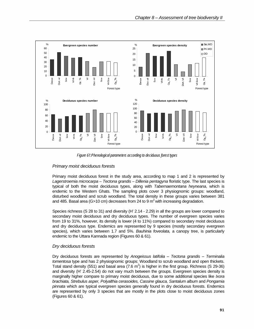
Figure 61:Phenological parameters according to deciduous forest types
Primary moist deciduous forests
Primary moist deciduous forest in the study area, according to map 1 and 2 is represented by Lagerstroemia microcarpa – Tectona grandis – Dillenia pentagyna floristic type. The last species is typical of both the moist deciduous types, along with Tabernaemontana heyneana, which is endemic to the Western Ghats. The sampling plots cover 3 physiognomic groups: woodland, disturbed woodland and scrub woodland. The total density in these groups varies between 381 and 485. Basal area (G>10 cm) decreases from 24 to 9 m2 with increasing degradation.
Species richness (S 28 to 31) and diversity (H’ 2.14 - 2.29) in all the groups are lower compared to secondary moist deciduous and dry deciduous types. The number of evergreen species varies from 19 to 31%, however, its density is lower (4 to 11%) compared to secondary moist deciduous and dry deciduous type. Endemics are represented by 9 species (mostly secondary evergreen species), which varies between 1.7 and 5%. Bauhinia foveolata, a canopy tree, is particularly endemic to the Uttara Kannada region (Figures 60 & 61).
Dry deciduous forests
Dry deciduous forests are represented by Anogeissus latifolia – Tectona grandis – Terminalia tomentosa type and has 2 physiognomic groups: Woodland to scrub woodland and open thickets. Total stand density (551) and basal area (7.6 m2) is higher in the first group. Richness (S 29-36) and diversity (H’ 2.45-2.54) do not vary much between the groups. Evergreen species density is marginally higher compare to primary moist deciduous, due to some additional species like Ixora brachiata, Strebulus asper, Polyalthia cerasoides, Cassine glauca, Santalum album and Pongamia pinnata which are typical evergreen species generally found in dry deciduous forests. Endemics are represented by only 3 species that are mostly in the plots close to moist deciduous zones (Figures 60 & 61).
Evergreen species number
010
2030
4050
60
Forest type
% Evergreen species density
0
5
10
15
20
25
Forest type
% Sec.MD
Pri.MD
DD
Deciduous species number
0
20
40
60
80
100
Forest type
% Deciduous species density
0
20
4060
80
100
120
Forest type
%
Chapter 8 – Assessment of tree biodiversity II
92
Impact of disturbance on structural parameters
Evergreen to semi evergreen forests
Spatial parameters like total density and basal area vary between and within the major types based on the degree of disturbance in the stand. Except in trMSA the mean number of species in all the types, is more than 50 Figure 58. Similarly, except in POIN and trMSA, the diversity (mean Shannon value) is between 2.6 and 3.33 irrespective of the physiognomic stage. The lower variability between these two is due to turnover in the rate of primary evergreen to secondary evergreen species with the increase in degradation.
Primary evergreen species number on average account for 62% in climax forests, gradually decreasing to 45% in non-climax forests and 27% in semi evergreen forests Figure 59. On the other hand, secondary evergreen species number, which are 29% in climax gradually increase to 36% in non-climax disturbed forests, and to 47%, further up in semi evergreen forests. The density of primary and secondary evergreen species also shows the same trend. Endemics show decline from 42% to 20% from climax to semi evergreen. Deciduous species, which occupy the openings, represent 9% in climax and increase to 13 in non-climax forests, and further show 3-fold increase in semi evergreen forests.
In ‘Kan’ forests, the number of secondary evergreen species (47) and its density (66) is higher compare to other wet evergreen types and the number of deciduous species is also higher except in semi evergreen forests.
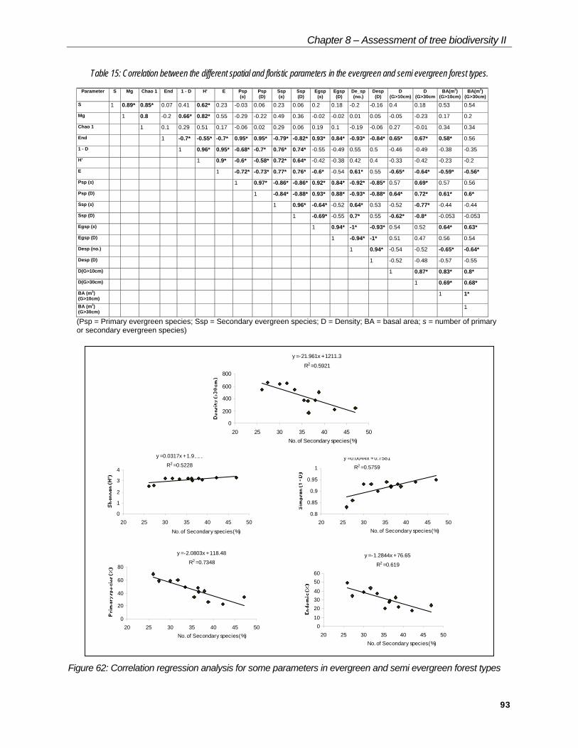
PCA and simple correlation analysis have shown that the secondary evergreen species is the most significant variable linked to several other parameters Table 15, Figure 62. On spatial structure, the increase in secondary species decreases the density of bigger trees (G>30 cm). Among floristic parameters, with the increase in secondary species, diversity (Shannon) and dominance (Simpson) are positively correlated, and primary and endemics are negatively correlated. On the contrary, an increase in primary species increases the endemics and density of big trees (G>30 cm).
Deciduous forests
In the deciduous types, the impact of disturbance has been generally reflected in the total basal area and density of big trees (G>30 cm), which show a decline with the increase in degradation. The overall decreases in evergreen species among the deciduous types is more related to climate rather than degradation. Richness and diversity show slight variation with degradation in each type (Figure 60).
In simple correlation analysis richness is positively associated with diversity. However, when the endemics are considered, there is a negatively correlated with the increase in deciduous species (Table 16, Figure 63). Among the deciduous species encountered in the study area, only Bauhinia foveolata and Tabernaemontana heyneana are endemics. Apart from these two, other endemics are evergreen, mainly found in secondary and primary moist deciduous types.
Chapter 8 – Assessment of tree biodiversity II
93
Table 15: Correlation between the different spatial and floristic parameters in the evergreen and semi evergreen forest types.
Parameter S Mg Chao 1 End 1 - D H' E Psp(s)
Psp(D)
Ssp(s)
Ssp(D)
Egsp(s)
Egsp(D)
De_sp(no.)
Desp(D)
D(G>10cm)
D(G>30cm
BA(m2)(G>10cm)
BA(m2)(G>30cm)
S 1 0.89* 0.85* 0.07 0.41 0.62* 0.23 -0.03 0.06 0.23 0.06 0.2 0.18 -0.2 -0.16 0.4 0.18 0.53 0.54
Mg 1 0.8 -0.2 0.66* 0.82* 0.55 -0.29 -0.22 0.49 0.36 -0.02 -0.02 0.01 0.05 -0.05 -0.23 0.17 0.2
Chao 1 1 0.1 0.29 0.51 0.17 -0.06 0.02 0.29 0.06 0.19 0.1 -0.19 -0.06 0.27 -0.01 0.34 0.34
End 1 -0.7* -0.55* -0.7* 0.95* 0.95* -0.79* -0.82* 0.93* 0.84* -0.93* -0.84* 0.65* 0.67* 0.58* 0.56
1 - D 1 0.96* 0.95* -0.68* -0.7* 0.76* 0.74* -0.55 -0.49 0.55 0.5 -0.46 -0.49 -0.38 -0.35
H' 1 0.9* -0.6* -0.58* 0.72* 0.64* -0.42 -0.38 0.42 0.4 -0.33 -0.42 -0.23 -0.2
E 1 -0.72* -0.73* 0.77* 0.76* -0.6* -0.54 0.61* 0.55 -0.65* -0.64* -0.59* -0.56*
Psp (s) 1 0.97* -0.86* -0.86* 0.92* 0.84* -0.92* -0.85* 0.57 0.69* 0.57 0.56
Psp (D) 1 -0.84* -0.88* 0.93* 0.88* -0.93* -0.88* 0.64* 0.72* 0.61* 0.6*
Ssp (s) 1 0.96* -0.64* -0.52 0.64* 0.53 -0.52 -0.77* -0.44 -0.44
Ssp (D) 1 -0.69* -0.55 0.7* 0.55 -0.62* -0.8* -0.053 -0.053
Egsp (s) 1 0.94* -1* -0.93* 0.54 0.52 0.64* 0.63*
Egsp (D) 1 -0.94* -1* 0.51 0.47 0.56 0.54
Desp (no.) 1 0.94* -0.54 -0.52 -0.65* -0.64*
Desp (D) 1 -0.52 -0.48 -0.57 -0.55
D(G>10cm) 1 0.87* 0.83* 0.8*
D(G>30cm) 1 0.69* 0.68*
BA (m2)(G>10cm)
1 1*
BA (m2)(G>30cm)
1
(Psp = Primary evergreen species; Ssp = Secondary evergreen species; D = Density; BA = basal area; s = number of primaryor secondary evergreen species)
y = -1.2844x + 76.65
R2 = 0.619
010
203040
5060
20 25 30 35 40 45 50 No. of Secondary species (%)
y = 0.0044x + 0.7581
R2 = 0.5759
0.8
0.85
0.9
0.95
1
20 25 30 35 40 45 50 No. of Secondary species (%)
y = 0.0317x + 1.9826
R2 = 0.5228
0
1
2
3
4
20 25 30 35 40 45 50
No. of Secondary species (%)
y = -2.0803x + 118.48
R2 = 0.7348
0
20
40
60
80
20 25 30 35 40 45 50 No. of Secondary species (%)
y = -21.961x + 1211.3
R2 = 0.5921
0
200
400
600
800
20 25 30 35 40 45 50 No. of Secondary species (%)
Figure 62: Correlation regression analysis for some parameters in evergreen and semi evergreen forest types

Chapter 8 – Assessment of tree biodiversity II
94
Table 16: Correlation between the different spatial and non-spatial parameters in deciduous forest types.
Parameter S Mg Chao 1 End 1 - D H' E Egsp(s) Egsp(D) Desp(s) Desp(D) D(G>10cm)
D(G>30cm)
D(G>60cm)
BA(m2)(G>10cm)
BA(m2)(G>30cm)
BA(m2)(G>60cm)
S 1 0.89* 0.82* 0.5 0.43 0.52 0.08 0.6* 0.5 -0.6* -0.5 0.27 0.29 0.21 0.15 0.14 0.12
Mg 1 0.87* 0.56 0.62* 0.76* 0.42 0.7* 0.7* -0.7* -0.7* -0.18 -0.08 -0.04 -0.05 -0.05 -0.03
Chao 1 1 0.45 0.26 0.43 0.07 0.5 0.5 -0.5 -0.5 -0.12 -0.03 0.09 0.06 0.07 0.1
Endemic 1 0.53 0.56 0.41 0.9* 0.7* -0.9* -0.7* -0.02 0.29 0.41 0.48 0.49 0.5
1 - D 1 0.96* 0.89* 0.5 0.7* -0.5 -0.7* -0.19 -0.13 -0.19 -0.24 -0.23 -0.24
H' 1 0.89* 0.6 0.8* -0.6 -0.8* -0.32 -0.24 -0.27 -0.29 -0.27 -0.27
E 1 0.4 0.7* -0.4 -0.7* -0.54 -0.44 -0.4 -0.38 -0.36 -0.33
Egsp(s) 1 -0.7* -1* 0.38 0 0.2 0.2 0.3 0.3 0.3
Egsp(D) 1 -0.8* -1* -0.4 -0.3 -0.3 -0.2 -0.2 -0.2
Desp(s) 1 0.8* 0 -0.1 -0.2 -0.3 -0.3 -0.3
Desp(D) 1 0.4 0.3 0.3 0.2 0.2 0.2
D(G>10cm) 1 0.83* 0.51 0.39 0.35 0.25
D(G>30cm) 1 0.87* 0.79* 0.77* 0.69*
D(G>60cm) 1 0.97* 0.97* 0.94*
BA(m2)(G>10cm)
1 1* 0.99*
BA(m2)(G>30cm)
1 0.96*
BA(m2)(G>60cm)
1
y = 0.2155x + 1.2839R2 = 0.5754
2
2.25
2.5
2.75
3
4 4.5 5 5.5 6 6.5 7 7.5 8
Richness (M g)
Div
ersi
ty (H
')
y = -0.4656x + 36.978R2 = 0.8421
0
2
4
6
8
10
12
14
16
40 50 60 70 80 90
Dec iduous spec ies (No.)
Ende
mic
s (%
)
Figure 63: Correlation regression analysis of some floristic parameters in deciduous forest types
Chapter 8 – Assessment of tree biodiversity II
95
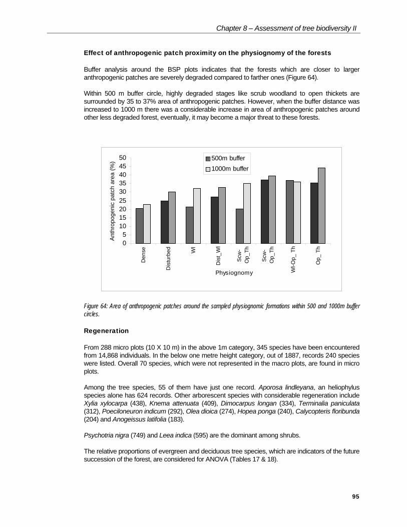
Effect of anthropogenic patch proximity on the physiognomy of the forests
Buffer analysis around the BSP plots indicates that the forests which are closer to larger anthropogenic patches are severely degraded compared to farther ones (Figure 64).
Within 500 m buffer circle, highly degraded stages like scrub woodland to open thickets are surrounded by 35 to 37% area of anthropogenic patches. However, when the buffer distance was increased to 1000 m there was a considerable increase in area of anthropogenic patches around other less degraded forest, eventually, it may become a major threat to these forests.
05
101520253035404550
Den
se
Dis
turb
ed Wl
Dis
t_W
l
Scw
-O
p_Th
Scw
-O
p_Th
Wl-O
p_ T
h
Op_
Th
Physiognomy
Anth
ropo
geni
c pa
tch
area
(%) 500m buffer
1000m buffer
Figure 64: Area of anthropogenic patches around the sampled physiognomic formations within 500 and 1000m buffer circles.
Regeneration
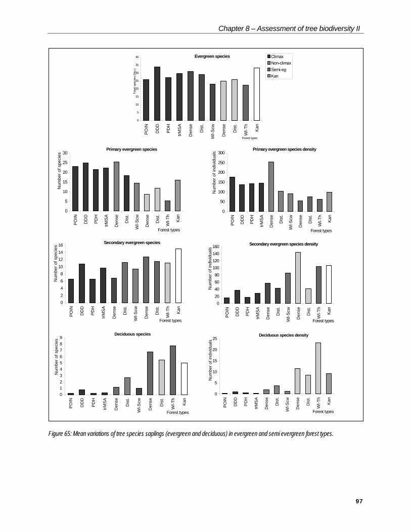
From 288 micro plots (10 X 10 m) in the above 1m category, 345 species have been encountered from 14,868 individuals. In the below one metre height category, out of 1887, records 240 species were listed. Overall 70 species, which were not represented in the macro plots, are found in micro plots.
Among the tree species, 55 of them have just one record. Aporosa lindleyana, an heliophylus species alone has 624 records. Other arborescent species with considerable regeneration include Xylia xylocarpa (438), Knema attenuata (409), Dimocarpus longan (334), Terminalia paniculata (312), Poeciloneuron indicum (292), Olea dioica (274), Hopea ponga (240), Calycopteris floribunda (204) and Anogeissus latifolia (183).
Psychotria nigra (749) and Leea indica (595) are the dominant among shrubs.
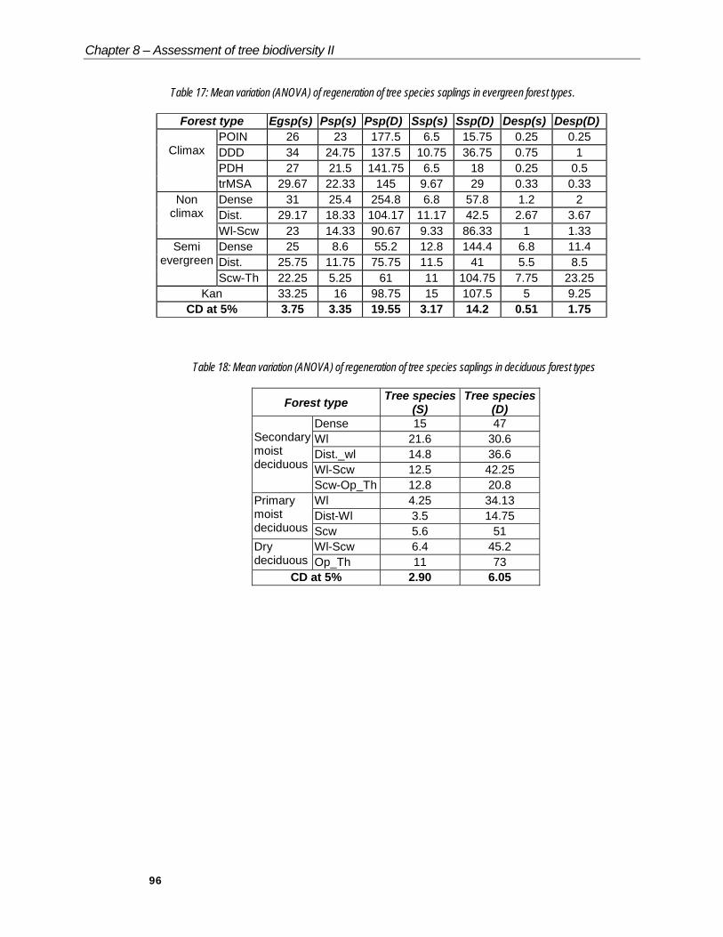
The relative proportions of evergreen and deciduous tree species, which are indicators of the future succession of the forest, are considered for ANOVA (Tables 17 & 18).
Chapter 8 – Assessment of tree biodiversity II
96
Table 17: Mean variation (ANOVA) of regeneration of tree species saplings in evergreen forest types.
Forest type Egsp(s) Psp(s) Psp(D) Ssp(s) Ssp(D) Desp(s) Desp(D)POIN 26 23 177.5 6.5 15.75 0.25 0.25DDD 34 24.75 137.5 10.75 36.75 0.75 1PDH 27 21.5 141.75 6.5 18 0.25 0.5
Climax
trMSA 29.67 22.33 145 9.67 29 0.33 0.33Dense 31 25.4 254.8 6.8 57.8 1.2 2Dist. 29.17 18.33 104.17 11.17 42.5 2.67 3.67
Nonclimax
Wl-Scw 23 14.33 90.67 9.33 86.33 1 1.33Dense 25 8.6 55.2 12.8 144.4 6.8 11.4Dist. 25.75 11.75 75.75 11.5 41 5.5 8.5
Semievergreen
Scw-Th 22.25 5.25 61 11 104.75 7.75 23.25Kan 33.25 16 98.75 15 107.5 5 9.25
CD at 5% 3.75 3.35 19.55 3.17 14.2 0.51 1.75
Table 18: Mean variation (ANOVA) of regeneration of tree species saplings in deciduous forest types
Forest type Tree species(S)
Tree species(D)
Dense 15 47Wl 21.6 30.6Dist._wl 14.8 36.6Wl-Scw 12.5 42.25
Secondarymoistdeciduous
Scw-Op_Th 12.8 20.8Wl 4.25 34.13Dist-Wl 3.5 14.75
Primarymoistdeciduous Scw 5.6 51
Wl-Scw 6.4 45.2Drydeciduous Op_Th 11 73
CD at 5% 2.90 6.05
Chapter 8 – Assessment of tree biodiversity II
97
Evergreen species
0
5
10
15
20
25
30
35
40
POIN
DD
D
PDH
trMSA
Den
se
Dis
t.
Wl-S
cw
Den
se
Dis
t.
Wl-T
h
Kan
Forest typesTo
tal s
peci
es (N
o.)
ClimaxNon-climaxSemi-egKan
Primary evergreen species
0
5
10
15
20
25
30
POIN
DD
D
PDH
trMSA
Den
se
Dis
t.
Wl-S
cw
Den
se
Dis
t.
Wl-T
h
Kan
Forest types
Num
ber o
f spe
cies
Secondary evergreen species
02468
10121416
POIN
DD
D
PDH
trMSA
Den
se
Dis
t.
Wl-S
cw
Den
se
Dis
t.
Wl-T
h
Kan
Forest types
Num
ber o
f spe
cies
Deciduous species
0123456789
PO
IN
DD
D
PD
H
trMS
A
Den
se
Dis
t.
Wl-S
cw
Den
se
Dis
t.
Wl-T
h
Kan
Forest types
Num
ber o
f spe
cies
Primary evergreen species density
0
50
100
150
200
250
300
POIN
DD
D
PDH
trMSA
Den
se
Dis
t.
Wl-S
cw
Den
se
Dis
t.
Wl-T
h
Kan
Forest types
Num
ber o
f ind
ivid
uals
Secondary evergreen species density
020406080
100120140160
POIN
DD
D
PDH
trMSA
Den
se
Dis
t.
Wl-S
cw
Den
se
Dis
t.
Wl-T
h
Kan
Forest types
Num
ber o
f ind
ivid
uals
Deciduous species density
0
5
10
15
20
25
PO
IN
DD
D
PD
H
trMS
A
Den
se
Dis
t.
Wl-S
cw
Den
se
Dis
t.
Wl-T
h
Kan
Forest types
Num
ber o
f ind
ivid
uals
Figure 65: Mean variations of tree species saplings (evergreen and deciduous) in evergreen and semi evergreen forest types.
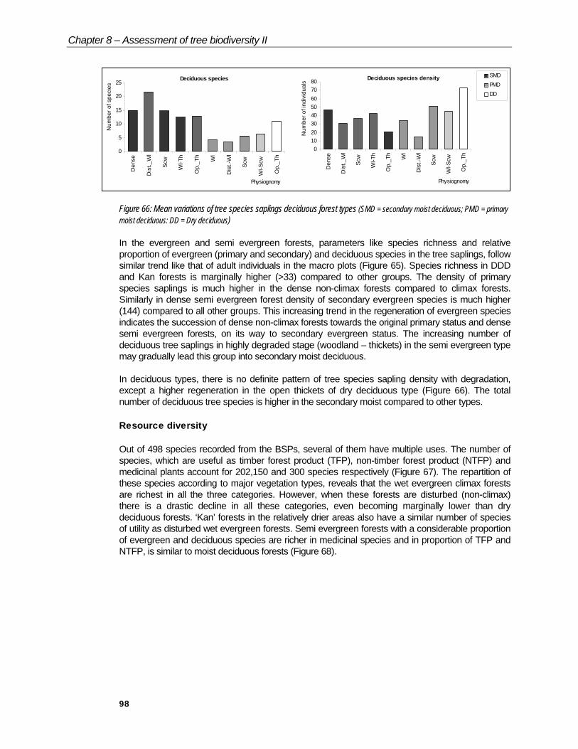
Chapter 8 – Assessment of tree biodiversity II
98
Deciduous species
0
5
10
15
20
25
Den
se
Dis
t._W
l
Scw
Wl-T
h
Op.
_Th
Wl
Dis
t.-W
l
Scw
Wl-S
cw
Op.
_Th
Physiognomy
Num
ber o
f spe
cies
Deciduous species density
01020304050607080
Den
se
Dis
t._W
l
Scw
Wl-T
h
Op.
_Th
Wl
Dis
t.-W
l
Scw
Wl-S
cw
Op.
_Th
Physiognomy
Num
ber o
f ind
ivid
uals
SMDPMDDD
Figure 66: Mean variations of tree species saplings deciduous forest types (SMD = secondary moist deciduous; PMD = primary moist deciduous: DD = Dry deciduous)
In the evergreen and semi evergreen forests, parameters like species richness and relative proportion of evergreen (primary and secondary) and deciduous species in the tree saplings, follow similar trend like that of adult individuals in the macro plots (Figure 65). Species richness in DDD and Kan forests is marginally higher (>33) compared to other groups. The density of primary species saplings is much higher in the dense non-climax forests compared to climax forests. Similarly in dense semi evergreen forest density of secondary evergreen species is much higher (144) compared to all other groups. This increasing trend in the regeneration of evergreen species indicates the succession of dense non-climax forests towards the original primary status and dense semi evergreen forests, on its way to secondary evergreen status. The increasing number of deciduous tree saplings in highly degraded stage (woodland – thickets) in the semi evergreen type may gradually lead this group into secondary moist deciduous.
In deciduous types, there is no definite pattern of tree species sapling density with degradation, except a higher regeneration in the open thickets of dry deciduous type (Figure 66). The total number of deciduous tree species is higher in the secondary moist compared to other types.
Resource diversity
Out of 498 species recorded from the BSPs, several of them have multiple uses. The number of species, which are useful as timber forest product (TFP), non-timber forest product (NTFP) and medicinal plants account for 202,150 and 300 species respectively (Figure 67). The repartition of these species according to major vegetation types, reveals that the wet evergreen climax forests are richest in all the three categories. However, when these forests are disturbed (non-climax) there is a drastic decline in all these categories, even becoming marginally lower than dry deciduous forests. ‘Kan’ forests in the relatively drier areas also have a similar number of species of utility as disturbed wet evergreen forests. Semi evergreen forests with a considerable proportion of evergreen and deciduous species are richer in medicinal species and in proportion of TFP and NTFP, is similar to moist deciduous forests (Figure 68).
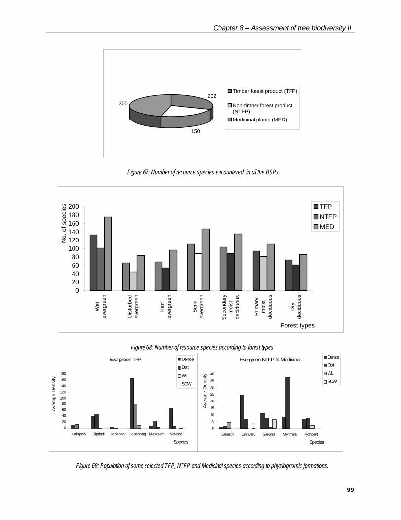
Chapter 8 – Assessment of tree biodiversity II
99
202
150
300
Timber forest product (TFP)
Non-timber forest product(NTFP)Medicinal plants (MED)
Figure 67: Number of resource species encountered in all the BSPs.
020406080
100120140160180200
Wet
ever
gree
n
Dis
turb
edev
ergr
een
Kan
'ev
ergr
een
Sem
iev
ergr
een
Sec
onda
rym
oist
deci
duou
s
Prim
ary
moi
stde
cidu
ous
Dry
deci
duou
s
Forest types
No.
of s
peci
es TFPNTFPMED
Figure 68: Number of resource species according to forest types
Evergreen TFP
020406080
100120140160180
Calopoly Diptindi Hopeparv Hopepong Mesuferr Vateindi
Species
Ave
rage
Den
sity
Dense
Dist
WL
SCW
Evergreen NTFP & Medicinal
0
510
15
20
2530
35
40
Canastri Cinnveru Garcindi Myrimala Hydnpent
Species
Ave
rage
Den
sity
Dense
Dist
WL
SCW
Figure 69: Population of some selected TFP, NTFP and Medicinal species according to physiognomic formations.
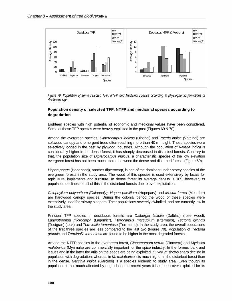
Chapter 8 – Assessment of tree biodiversity II
100
Deciduous TFP
0
20
40
60
80
100
120
Dalblati Lagemicr Ptermars Tectgran Termtome
Species
Ave
rage
Den
sity
WLDist_WLSCWWL-op_Th
Deciduous NTFP & Medicinal
0
2
4
6
8
10
12
Emberibe Embloffi HolaantiSpecies
Ave
rage
Den
sity
WLDist_WLSCWWL-op_Th
Figure 70: Population of some selected TFP, NTFP and Medicinal species according to physiognomic formations of deciduous type
Population density of selected TFP, NTFP and medicinal species according to degradation
Eighteen species with high potential of economic and medicinal values have been considered. Some of these TFP species were heavily exploited in the past (Figures 69 & 70).
Among the evergreen species, Dipterocarpus indicus (Diptindi) and Vateria indica (Vateindi) are softwood canopy and emergent trees often reaching more than 40-m height. These species were selectively logged in the past by plywood industries. Although the population of Vateria indica is considerably higher in the dense forest, it has sharply decreased in disturbed forests. Contrary to that, the population size of Dipterocarpus indicus, a characteristic species of the low elevation evergreen forest has not been much altered between the dense and disturbed forests (Figure 69).
Hopea ponga (Hopepong), another dipterocarp, is one of the dominant under-storey species of the evergreen forests in the study area. The wood of this species is used extensively by locals for agricultural implements and furniture. In dense forest its average density is 165, however, its population declines to half of this in the disturbed forests due to over exploitation.
Calophyllum polyanthum (Caloppoly), Hopea parviflora (Hopeparv) and Mesua ferrea (Mesuferr) are hardwood canopy species. During the colonial period the wood of these species were extensively used for railway sleepers. Their populations severely dwindled, and are currently low in the study area.
Principal TFP species in deciduous forests are Dalbergia latifolia (Dalblati) (rose wood), Lagerstroemia microcarpa (Lagemicr), Pterocarpus marsupium (Ptermars), Tectona grandis (Tectgran) (teak) and Terminalia tomentosa (Termtome). In the study area, the overall populations of the first three species are less compared to the last two (Figure 70). Population of Tectona grandis and Terminalia tomentosa are found to be higher in the most degraded forests.
Among the NTFP species in the evergreen forest, Cinnamomum verum (Cinnveru) and Myristica malabarica (Myrimala) are commercially important for the spice industry. In the former, bark and leaves and in the latter the arils on the seeds are being exploited. C. verum shows sharp decline in population with degradation, whereas in M. malabarica it is much higher in the disturbed forest than in the dense. Garcinia indica (Garcindi) is a species endemic to study area. Even though its population is not much affected by degradation, in recent years it has been over exploited for its
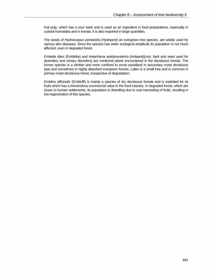
Chapter 8 – Assessment of tree biodiversity II
101
fruit pulp, which has a sour taste and is used as an ingredient in food preparations, especially in coastal Karnataka and in Kerala. It is also exported in large quantities.
The seeds of Hydnocarpus pentandra (Hydnpent) an evergreen tree species, are widely used for various skin diseases. Since the species has wider ecological amplitude its population is not much affected, even in degraded forest.
Embelia ribes (Emblribe) and Holarrhena antidysenterica (Holaanti)(root, bark and seed used for dysentery and urinary disorders) are medicinal plants encountered in the deciduous forests. The former species is a climber and more confined to scrub woodland in secondary moist deciduous type and sometimes in highly disturbed evergreen forests. Latter is a small tree and is common in primary moist deciduous forest, irrespective of degradation.
Emblica officinalis (Embloffi) is mainly a species of dry deciduous forests and is exploited for its fruits which has a tremendous commercial value in the food industry. In degraded forest, which are closer to human settlements, its population is dwindling due to over-harvesting of fruits, resulting in low regeneration of this species.

102
Assessment of tree biodiversity: Part III Comments on the outcome of analyses
Discussion
The Western Ghats of Karnataka
Despite the high rainfall, the Karnataka part of the Western Ghats (KWG) is floristically less diverse compared to its counterpart in Kerala state due to longer dry period (4 – 7 months). The vegetation map prepared by the FIP reveals that KWG represent 14 climax types, with tree species richness, especially in the evergreen types, varying between 92 – 166 species. Whereas, the southern parts have 16 types with high numbers of species (ranging from 260 to 380). The low richness in KWG also reflects in the BSPs, where only 498 species have been encountered from nearly 100,000 records. A comparison with the ≥1-ha sampling plots in the southern part of the Western Ghats shows that even at the limit of ≥10 DBH (diameter at breast height) the species richness and basal area is considerably lower in the present study area (Table 19). When compared to some of the neotropical and south-east Asian forests, the species richness in BSPs is far lower (Table 19).
The Western Ghats is one of the ‘mega centres’ of endemism (Nayar, 1996). Nearly 56% of the total evergreen species (650) found here are endemic to the Ghats. Length of the dry season is an important factor in the distribution of endemics (Ramesh & Pascal, 1997). With a higher number of dry months, KWG accounts for nearly 171 of the total endemics (352). Species like Bauhinia foveolata, Garcinia indica, Mamea suriga, Hopea canarensis, Hopea jacobi are exclusive to KWG.
In spite of climatic constraints, KWG is unique in several ways. The Kodagu region (the southern part of KWG) where the length of dry season is around 4 months is as rich as southern part of the Western Ghats. It acts like a transition zone, with the presence of certain typical species of the southern part, which are generally adopted to shorter dry period like Dipterocarpus bourdillonii, Semecarpus auriculata, Diospyros nilagirica, Diospyros bourdillonii on one hand and on the other some of the typical species adapted to a longer dry period like Garcinia indica, Diospyros oocarpa, Diospyros buxifolia. Unfortunately the BSP do not cover this region in the current phase. However, permanent plots (around 5-ha) established by FIP reveal that the low elevation evergreen forest is nearly as rich as similar forests in the south (Table 19) (Pascal & Pelissier, 1996).
The Western Ghats are the western-most limit of the dipterocarp domain (Ramesh et al., 1996). Due to high population pressures in Kerala State, the low elevation dipterocarp forests are severely fragmented (Ramesh et al., 1997). Currently, the best parts of the dipterocarp forest lie in the KWG.
Poeciloneuron, one of the few endemic genera in the Western Ghats, has 2 species. P. pauciflorum is endemic to extreme southern part of the Western Ghats (Ramesh & Pascal, 1997) Where as P. indicum is patchily distributed throughout the Ghats. However, in KWG it nearly becomes monodominant, in very high rainfall zones (>5000 mm).
Chapter
9

Chapter 9 – Assessment of tree biodiversity III
103
Table 19: Density, Basal area and species richness recorded in 1-ha or more size of plots in the evergreenforests of the Western Ghats of India and other parts of tropics.
Site
Plot
siz
e(h
a)
Alti
tude
(m)
Rai
nfal
l
(mm
)
Den
sity
(>10
DB
H)
Bas
alA
rea
(m2 )
No.
of
spec
ies
Sour
ce
SengaltheriKalakadTamil Nadu
1 1170 3000 720 55.3 95 Parthasarathy,1999
KakachiKalakadTamil Nadu
3.82 1250-1450
3000 582.7 42.03 90 Ganesh et al.,1996
NelliampathyKerala
1 950 496 61.9 30 Chandrasekar,a 1994
Uppangala,Karnataka
3.12 500 5100 635 (ha-1) 40 (ha-1) 91 Pascal &Pelissier, 1996
BSP24(ID73) 1 640 >5000 976 32 53BSP26(ID74) 1 680 >5000 535 41 44BSP28(ID66) 1 1060 >5000 376 60 21BSP53(ID80) 1 520 2000-
5000683 29 56
BSP51(ID83) 1 540 2000-5000
710 29 51
PSPLD3(ID6) 1 500 2000-5000
480 32 56
BSP54(ID84) 1 55 2000-5000
755 32 73
BSPNK4(ID88) 1 160 2000-5000
660 40 50
BSPNK6(ID89) 1 390 >5000 619 29 49BSPNK4(ID90) 1 615 2000-
5000609 33 38
Wes
tern
Gha
ts
BSPNK8(ID91) 1 610 >5000 751 28 34
Present study(only leastdisturbed plotsthat belong toclimax evergreenforests are givenin this table)
AmasoniaEcuador
260 3.5 693 30 Valencia et al.,1994
MishanaPeru
1 140 3000 858 289 Gentry, 1988b
ChocoColombia
1 100 675 258 Faber-Langendoenand Gentry,1991
CMBRSPNG
1 900 6400 693 228 Wright et al.,1997
Gunung MuluSarawak
1 200 5100 778 214 Proctor et al.,1983
PasohMalaysia
1 200 2000 530 210 Kochummen etal., 1990
Cocha CashuPeru
1 100 2000 673 201 Gentry andTerborgh,1990
QueenlandAustralia
1 730 2000 957 108 Phillips et al.,1994
La SelvaCosta Rica
1 100 4000 447 96 Lieberman etal., 1985
BCIPanama
1 10 2500 414 93 Gentry, 1990
Neo
-trop
ics
and
sout
h-ea
st A
sia
AmazonVenezuela
1 100 3500 744 83 Uhl andMurphy, 1981
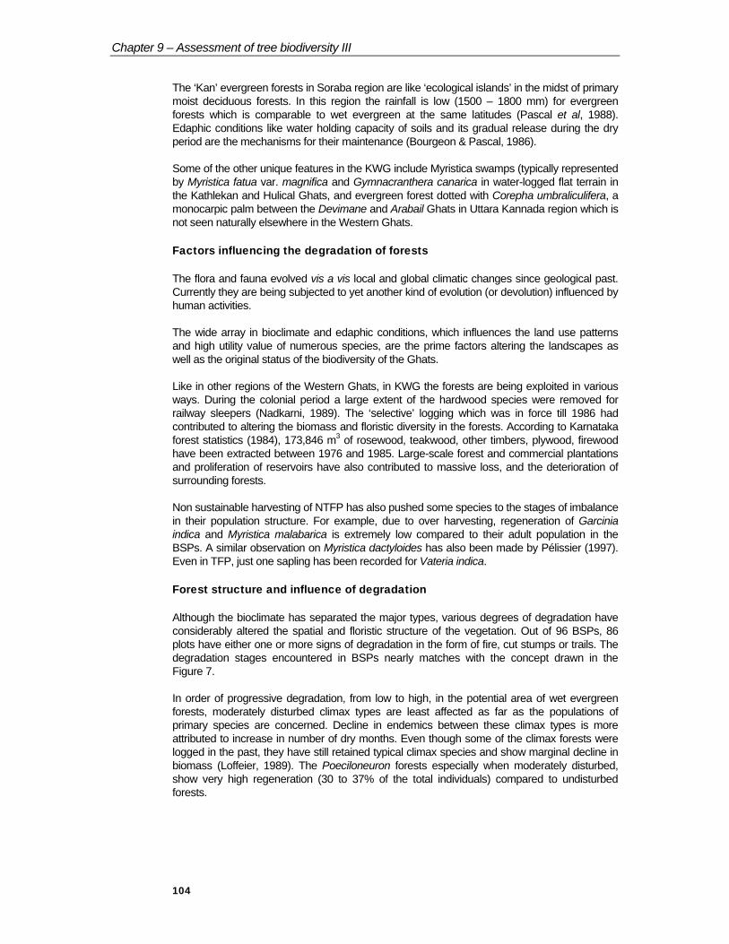
Chapter 9 – Assessment of tree biodiversity III
104
The ‘Kan’ evergreen forests in Soraba region are like ‘ecological islands’ in the midst of primary moist deciduous forests. In this region the rainfall is low (1500 – 1800 mm) for evergreen forests which is comparable to wet evergreen at the same latitudes (Pascal et al, 1988). Edaphic conditions like water holding capacity of soils and its gradual release during the dry period are the mechanisms for their maintenance (Bourgeon & Pascal, 1986).
Some of the other unique features in the KWG include Myristica swamps (typically represented by Myristica fatua var. magnifica and Gymnacranthera canarica in water-logged flat terrain in the Kathlekan and Hulical Ghats, and evergreen forest dotted with Corepha umbraliculifera, a monocarpic palm between the Devimane and Arabail Ghats in Uttara Kannada region which is not seen naturally elsewhere in the Western Ghats.
Factors influencing the degradation of forests
The flora and fauna evolved vis a vis local and global climatic changes since geological past. Currently they are being subjected to yet another kind of evolution (or devolution) influenced by human activities.
The wide array in bioclimate and edaphic conditions, which influences the land use patterns and high utility value of numerous species, are the prime factors altering the landscapes as well as the original status of the biodiversity of the Ghats.
Like in other regions of the Western Ghats, in KWG the forests are being exploited in various ways. During the colonial period a large extent of the hardwood species were removed for railway sleepers (Nadkarni, 1989). The ‘selective’ logging which was in force till 1986 had contributed to altering the biomass and floristic diversity in the forests. According to Karnataka forest statistics (1984), 173,846 m3 of rosewood, teakwood, other timbers, plywood, firewood have been extracted between 1976 and 1985. Large-scale forest and commercial plantations and proliferation of reservoirs have also contributed to massive loss, and the deterioration of surrounding forests.
Non sustainable harvesting of NTFP has also pushed some species to the stages of imbalance in their population structure. For example, due to over harvesting, regeneration of Garcinia indica and Myristica malabarica is extremely low compared to their adult population in the BSPs. A similar observation on Myristica dactyloides has also been made by Pélissier (1997). Even in TFP, just one sapling has been recorded for Vateria indica.
Forest structure and influence of degradation
Although the bioclimate has separated the major types, various degrees of degradation have considerably altered the spatial and floristic structure of the vegetation. Out of 96 BSPs, 86 plots have either one or more signs of degradation in the form of fire, cut stumps or trails. The degradation stages encountered in BSPs nearly matches with the concept drawn in the Figure 7.
In order of progressive degradation, from low to high, in the potential area of wet evergreen forests, moderately disturbed climax types are least affected as far as the populations of primary species are concerned. Decline in endemics between these climax types is more attributed to increase in number of dry months. Even though some of the climax forests were logged in the past, they have still retained typical climax species and show marginal decline in biomass (Loffeier, 1989). The Poeciloneuron forests especially when moderately disturbed, show very high regeneration (30 to 37% of the total individuals) compared to undisturbed forests.

Chapter 9 – Assessment of tree biodiversity III
105
However, when these forests are repeatedly logged, the typical climax species either disappear or become very rare. Thus, the forest becomes “non-climax”. Further heavy exploitation of these disturbed forests may result in woodland to scrub woodland stages or it may gradually turn into semi evergreen with the colonisation of deciduous species in the openings and finally to secondary moist deciduous formations with the increasing anthropogenic pressures. Daniels et al. (1995) in Uttara Kannada also observed a similar tendency in their studies along the gradient of disturbance.
It is possible that with protection, some of the non-climax forests and semievergreen forests are in the process of recovery, as manifested in their high density in the lower girth classes and also in regeneration. A relatively high basal area in disturbed non-climax forests may be attributed to low competition and availability of ample space for the remaining big trees after early stages of disturbance.
In terms of total species richness and diversity there is no big difference between climax, non-climax and semi evergreen forests. Even the degradation of the latter two has not severely affected the richness and diversity. Although the biomass has been altered. However, when the qualitative nature of the species composition are considered, there is a decline in the proportion of primary evergreen species and concomitant increase in the secondary evergreen species. As 95% of the endemic species are primary, their decline with the degradation is obvious.
‘Kan’ evergreen forests are naturally characterised by high proportion of secondary species like Aporosa lindleyana, Xantolis tomentosa, Flacourtia montana, Ixora brachiata, Holigarna grahamii, Olea dioica, Vitex altissima. In addition to climatic constraints ‘Kans’ are highly threatened by anthropogenic pressures from the surrounding human habitation. This has already been reflected in the increasing number of deciduous species, which may eventually push this unique ecosystem into moist deciduous forms.
Primary moist and dry deciduous forests are also not affected in terms of total richness and diversity with the disturbance. However, a big difference lies in the decrease in biomass in the form of density of big trees and basal area with the increase in degradation.
The relative proportions of primary and secondary evergreen and deciduous species are the most important indicators of the qualitative changes in the biodiversity. Several primary species like Hopea canarensis, Cleistanthus malabaricus, Casearia wynadensis have restricted distributions. The disappearance of these species may result in either extirpation or extinction of one or more species on this planet. Climax evergreen forests are not only ecologically significant with the high rates of endemism but also the gene banks of several economically and medicinally important species. In consideration of these factors, climax evergreen forests are the high priority areas for conservation.

106
A case study of logging impact Floristic composition and structure of a low elevation wet evergreen forest
Kadamakal Reserve Forest, Kodagu District
Introduction
Forest management rests upon knowledge of floristic composition and structure as well as on forest dynamics and functioning. With the intention of providing these tools to be used in decision-making for the management of the forest, studies have been conducted in a low elevation wet evergreen forest of the Western Ghats of Karnataka, in Kodagu District. This was done in collaboration with the Karnataka Forest Department.
Presentation of the study site
The experimental station is located within a 28 ha area of undisturbed forest in the Kadamakal Reserve Forest of the Kodagu District, near the village of Uppangala (12°30'N; 75°39'E), at an elevation that ranges from 400 to 600 m above sea level. The Kadamakal Reserve Forest comes under the Dipterocarpus indicus - Kingiodendron pinnatum - Humboldtia brunonis type of the low elevation dense wet evergreen forests of this region. Annual rainfall is about 5200 mm with a marked dry season of 3-4 months, from December to March. The mean annual temperature is 27°C, and the minimum mean temperature of about 25°C coincides with the rainfall peak in July.
Floristic composition and structure
The experimental station, first surveyed in 1990, comprises transects that are 20 m wide, 180 to 370 m long and 100 m apart. This constitutes a systematic sample of 3.12 ha and rectangular plots devoted to the study of the forest mosaic and spatial distribution (Figure 71). In each plot, all the trees with girth at breast height (gbh) above 30 cm were recorded, numbered, and identified.
Forest structure
In the five bands (3.12 ha), 1981 trees of girth size above 30 cm were recorded. The mean density was 635 trees per ha and the basal area 123.8 m2, i.e. 39.7 m2 per ha (Pascal & Pélissier, 1996). The distribution of girth classes follows the classic negative exponential pattern found in undisturbed rainforests (Fig. 72).
Chapter
10
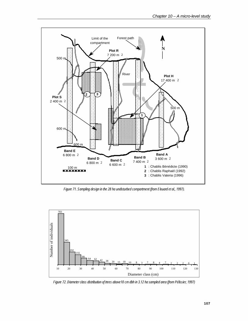
Chapter 10 – A micro-level study
107
Band E6 800 m 2
Band D6 800 m 2 Band C
6 600 m 2
Band B7 400 m 2
Band A3 600 m 2
1 : Chablis Bénédicte (1990)2 : Chablis Raphaël (1992)3 : Chablis Vateria (1996)
100 m
600 m
600 m
500 m
Limit of thecompartment
River
2
Plot H17 400 m 2
1
Forest path
Plot R7 200 m 2
N
Plot S2 400 m 2
500 m
3
Figure 71. Sampling design in the 28 ha undisturbed compartment (from Elouard et al., 1997).
20 10227 247 88 318 10152862 4264
99155
192
783
10 20 30 40 50 60 70 80 90 100 110 120 130
Num
ber o
f ind
ivid
uals
Diameter class (cm)
345
Figure 72. Diameter class distribution of trees above10 cm dbh in 3.12 ha sampled area (from Pélissier, 1997)

Chapter 10 – A micro-level study
108
Floristic composition, richness and diversity
The north-south bands established throughout the compartment aim at providing a good statistical frequency of the site with an assessment of species diversity. A total of 91 species belonging to 31 families were recorded within the five bands. However, 12 species recorded in this forest were not observed in the sampled area. The well-represented families are Euphorbiaceæ (20 species), Anacardiaceæ (7), Lauraceæ, Ebenaceæ and Meliaceæ (6 species each), Dipterocarpaceæ, Annonaceæ and Clusiaceæ (5 each). The Dipterocarpaceæ is the most represented family in individuals, constituting 21.1% of the stand in terms of relative density of trees. Myristicaceæ, represented by 3 species, and Fabaceæ, represented by 2 species, constitute 19.4% and 15.9% respectively of the total individuals. Half of the species (48%) are endemics to the Western Ghats, and about 80% of the trees belong to these endemic species.
The Simpson’s diversity index (D) is equal to 0.92 and the Shannon index (H)' is 4.56 for a maximum diversity (H max) of 6.54 and an equitability (E) of 0.70. The floristic structure, studied by the Importance Value Index IVIr was calculated based upon relative density and relative basal area, without taking the relative occurrence in the quadrats, rF, into account (IVI* = rD + rBA). The total value IVI* for all the species is 200, and it is rapidly decreasing, with values below 25 for the second species, below 15 for the fifth species and below 5 beyond the tenth species.
The dominant families are Dipterocarpaceæ (IVI*=63.3), Myristicaceæ (35.9) and Fabaceæ (23.2). The dominant species are Vateria indica L. (IVI*=46.0), Myristica dactyloïdes Gaertn. (24.6), Humboldtia brunonis Wall. (17.6) and Dipterocarpus indicus Bedd. (15.0) (Figure 73). These four species represent more than 48% of the individuals and 55% of the basal area. The first three species represent more than 45% of the effective (Vateria indica, 16.7%; Myristica dactyloïdes, 13.2% and Humboldtia brunonis, 11.4%). The most important basal area is shown by Vateria indica (29.3%), Dipterocarpus indicus (12.1%) and Myristica dactyloïdes (11.4%).
There are 56 rare or low frequency species (maximum 2 individuals per hectare), representing two-third of the inventoried species (Pélissier, 1997). The species richness is not very high, but diversity is high due to the fact that a few species are very abundant and a large number of species are rare or with low frequency.
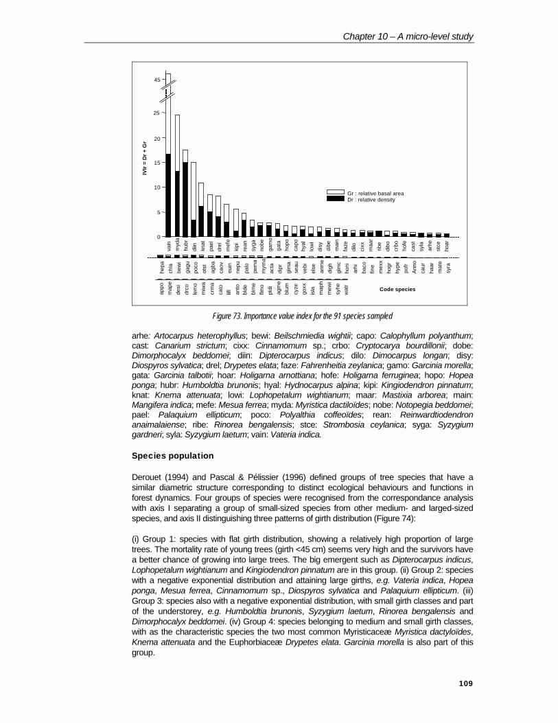
Chapter 10 – A micro-level study
109
Gr : relative basal areaDr : relative density
IVIr
= D
r + G
r
Code species
0
5
10
20
15
25
45
vain
m
yda
hubr
di
in
knat
pa
el
drel
m
efe
kipi
re
an
syga
no
be
gam
o ga
ta
hopo
capo
hy
al
low
i di
sy
dibe
m
ain
faze
di
lo
cixx
m
aar
ribe
dibo
cr
bo
hofe
ca
st
syla
ar
he
stce
ho
ar
hepa
ch
la
bew
i ga
gu
poco
ot
st
agba
ca
ov
euin
ne
pu
palo
pe
ma
mym
a ac
ta
dipr
gl
ma
seau
ve
bi
else
an
me
digh
gl
mc
honi
ar
hi
baco
fin
e m
exx
hogr
hy
pe
pofr
Ann
o ca
ur
haar
m
ate
syra
appo
m
ape
desi
dr
co
lem
o m
iwa
crm
a ca
to
lifl
anto
bl
de
blm
e flm
o pt
di
agm
e bl
um
cyze
go
xx
isla
m
aph
mew
i sy
he
wat
r
Figure 73. Importance value index for the 91 species sampled
arhe: Artocarpus heterophyllus; bewi: Beilschmiedia wightii; capo: Calophyllum polyanthum; cast: Canarium strictum; cixx: Cinnamomum sp.; crbo: Cryptocarya bourdillonii; dobe: Dimorphocalyx beddomei; diin: Dipterocarpus indicus; dilo: Dimocarpus longan; disy: Diospyros sylvatica; drel; Drypetes elata; faze: Fahrenheitia zeylanica; gamo: Garcinia morella; gata: Garcinia talbotii; hoar: Holigarna arnottiana; hofe: Holigarna ferruginea; hopo: Hopea ponga; hubr: Humboldtia brunonis; hyal: Hydnocarpus alpina; kipi: Kingiodendron pinnatum; knat: Knema attenuata; lowi: Lophopetalum wightianum; maar: Mastixia arborea; main: Mangifera indica; mefe: Mesua ferrea; myda: Myristica dactiloïdes; nobe: Notopegia beddomei; pael: Palaquium ellipticum; poco: Polyalthia coffeoïdes; rean: Reinwardtiodendron anaimalaiense; ribe: Rinorea bengalensis; stce: Strombosia ceylanica; syga: Syzygium gardneri; syla: Syzygium laetum; vain: Vateria indica. Species population
Derouet (1994) and Pascal & Pélissier (1996) defined groups of tree species that have a similar diametric structure corresponding to distinct ecological behaviours and functions in forest dynamics. Four groups of species were recognised from the correspondance analysis with axis I separating a group of small-sized species from other medium- and larged-sized species, and axis II distinguishing three patterns of girth distribution (Figure 74):
(i) Group 1: species with flat girth distribution, showing a relatively high proportion of large trees. The mortality rate of young trees (girth <45 cm) seems very high and the survivors have a better chance of growing into large trees. The big emergent such as Dipterocarpus indicus, Lophopetalum wightianum and Kingiodendron pinnatum are in this group. (ii) Group 2: species with a negative exponential distribution and attaining large girths, e.g. Vateria indica, Hopea ponga, Mesua ferrea, Cinnamomum sp., Diospyros sylvatica and Palaquium ellipticum. (iii) Group 3: species also with a negative exponential distribution, with small girth classes and part of the understorey, e.g. Humboldtia brunonis, Syzygium laetum, Rinorea bengalensis and Dimorphocalyx beddomei. (iv) Group 4: species belonging to medium and small girth classes, with as the characteristic species the two most common Myristicaceæ Myristica dactyloïdes, Knema attenuata and the Euphorbiaceæ Drypetes elata. Garcinia morella is also part of this group.

Chapter 10 – A micro-level study
110
crbo
arhe
capo
cast
cixxdibe
diin
dilo
disy
drelgamohoar
hofe
hopo
hubr
kipi
knat
lowi
mefe
myda
nobe
pael
poco
ribe
syga
syla
vain
fazebewi maarstcerean
gatahyal
F2
Group 1
Group 2
Group 4
Group 3
main
F1
Diameter c lasses (cm)
0
0,1
0,2
0,3
10 30 50 70 90 110
0
0,1
0,2
0,3
10 30 50 70 90 110
Myristica dactyloïdes
0
0,1
0,2
10 30 50 70
Dipterocarpus indicusVateria indica
Humboldtia brunonis
0
0,1
0,9
10 30
0,1
0,2
0,3
10 30 50 700
Knema attenuata
0
0,1
0,2
10 30 50 70
Drypetes elata
Diameter c lasses (cm)
Diameter c lasses (cm)
Rel
ativ
e fre
quen
cyR
elat
ive
frequ
ency
Rel
ativ
e fre
quen
cy
Figure 74. Correspondance analysis performed on the girth class distributions of 35 species (frequency >2
trees/ha) and examples of distributions corresponding to the four identified groups (from Pélissier, 1997).
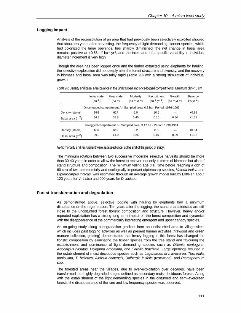
Chapter 10 – A micro-level study
111
Logging impact
Analysis of the reconstitution of an area that had previously been selectively exploited showed that about ten years after harvesting, the frequency of light-demanding pioneer species, which had colonized the large openings, has sharply diminished; the net change in basal area remains positive at +0.56 m2 ha-1 yr-1, and the inter- and infra-specific variability in individual diameter increment is very high.
Though the area has been logged once and the timber extracted using elephants for hauling, the selective exploitation did not deeply alter the forest structure and diversity, and the recovery in biomass and basal area was fairly rapid (Table 20) with a strong stimulation of individual growth.
Table 20: Density and basal area balance in the undisturbed and once-logged compartments. Minimum dbh=10 cm
Initial state(ha-1)
Final state(ha-1)
Mortality(ha-1.yr-1)
Recruitment(ha-1.yr-1)
Growth(ha-1.yr-1)
Balance(%.yr-1)
Once-logged compartment A - Sampled area: 0.6 ha - Period: 1986-1993Density (stems) 578 617 5.0 10.5 — +0.95
Basal area (m2) 34.8 38.8 0.40 0.10 0.86 +1.61
Unlogged compartment B - Sampled area: 3.12 ha - Period: 1990-1994Density (stems) 606 619 5.2 8.5 — +0.54
Basal area (m2) 39.3 41.0 0.26 0.07 0.59 +1.02
Note: mortality and recruitment were assessed once, at the end of the period of study.
The minimum rotation between two successive moderate selective harvests should be more than 30-40 years in order to allow the forest to recover, not only in terms of biomass but also of stand structure and composition. The minimum felling age (i.e., time before reaching a dbh of 60 cm) of two commercially and ecologically important dipterocarp species, Vateria indica and Dipterocarpus indicus, was estimated through an average growth model built by Loffeier: about 120 years for V. indica and 200 years for D. indicus.
Forest transformation and degradation
As demonstrated above, selective logging with hauling by elephants had a minimum disturbance on the regeneration. Ten years after the logging, the stand characteristics are still close to the undisturbed forest floristic composition and structure. However, heavy and/or repeated exploitation has a strong long term impact on the forest composition and dynamics with the disappearance of the commercially interesting emergent and upper canopy species.
An on-going study along a degradation gradient from an undisturbed area to village sites, which includes past logging activities as well as present human activities (firewood and green manure collection, grazing) demonstrates that heavy logging in this forest has changed the floristic composition by eliminating the timber species from the tree stand and favouring the establishment and dominance of light demanding species such as Dillenia pentagyna, Artocarpus hirsutus, Holigarna arnottiana, and Carallia brachiata. Large openings resulted in the establishment of moist deciduous species such as Lagerstroemia microcarpa, Terminalia paniculata, T. bellerica, Albizzia chinensis, Dalbergia latifolia (rosewood), and Pterospermum spp.
The forested areas near the villages, due to over-exploitation over decades, have been transformed into highly degraded stages defined as secondary moist deciduous forests. Along with the establishment of the light demanding species in the disturbed and semi-evergreen forests, the disappearance of the rare and low frequency species was observed.

Chapter 10 – A micro-level study
112
Along this gradient, the regenerative stand in the disturbed and semi-evergreen forests has shown a potential for rehabilitation of the primary forest. On the other hand, the regenerative stand in the forest areas heavily exploited in the past and presently degraded by human activities is poor and devoid of evergreen species. Degradation is at a level too high to allow rehabilitation of the original forest type.
This phenomenon may also occur when secondary forest products are over-exploited for commercial purposes, in an unsustainable manner. Local people collect the fruits of Myristica dactyloides (Myristicaceae) to derive a yellowish dye. This species is one of the four most common trees species and the collection of these fruits impoverishes the regenerative pool of the species. Eventually, a change of the forest composition and structure may occur and various scenarios can be envisaged: either one species will take over the position of M. dactyloides in the tree population, or several species will increase their respective occurrence.
Conclusion
The Kadamakal Reserve Forest is one of the rare well-preserved sites of low elevation evergreen forest in the Western Ghats. Though species richness is not very high compared to other forest sites, the high species diversity with the dominance of four species shows peculiar characteristics of the forest structure. Topography, which varies from 15 to 40 degrees of slope, plays an important role in the spatial distribution of the trees. Various studies on regeneration, spatial distribution, phenology, architecture and regenerative processes in tree-fall gaps have built up knowledge of the dynamics and functioning of this forest type. This knowledge allows defining tools for biodiversity conservation as well as rehabilitation of degraded areas.
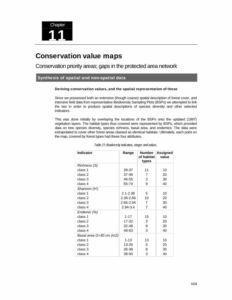
113
Conservation value maps Conservation priority areas; gaps in the protected area network
Synthesis of spatial and non-spatial data
Deriving conservation values, and the spatial representation of these
Since we possessed both an extensive (though coarse) spatial description of forest cover, and intensive field data from representative Biodiversity Sampling Plots (BSPs) we attempted to link the two in order to produce spatial descriptions of species diversity and other selected indicators.
This was done initially by overlaying the locations of the BSPs onto the updated (1997) vegetation layers. The habitat types thus covered were represented by BSPs, which provided data on tree species diversity, species richness, basal area, and endemics. The data were extrapolated to cover other forest areas classed as identical habitats. Ultimately, each point on the map, covered by forest types had these four attributes.
Table 21: Biodiversity indicators, ranges and values.
Indicator Range Numberof habitat
types
Assignedvalue
Richness (S)class 1 28-37 11 10class 2 37-46 7 20class 3 46-55 2 30class 4 55-74 9 40Shannon (H')class 1 2.1-2.38 5 10class 2 2.38-2.66 10 20class 3 2.66-2.94 7 30class 4 2.94-3.4 7 40Endemic (%)class 1 1-17 15 10class 2 17-32 3 20class 3 32-48 8 30class 4 48-63 3 40Basal area G>30 cm (m2)class 1 1-13 13 10class 2 13-26 5 20class 3 26-38 8 30class 4 38-50 3 40
Chapter
11

Chapter 11 - Conservation value maps
114
Table 22: Indicator sum values, areas, and conservation value classes.
sum Number of patches Area (ha) Area (km2) Conservation value class
40 205 34,537.5 345.4 150 641 328,458.2 3,284.6 160 1090 283,686.6 2,836.9 170 0 0 0.0 280 776 112,709.6 1,127.1 290 1208 151,810.2 1,518.1 3100 6 975.345 9.8 3110 22 15,218.7 152.2 4120 0 0 0.0 4130 1244 236,846.2 2,368.5 4140 72 20,026.4 200.3 5150 50 27,031.1 270.3 5160 0 0 0.0 5
Forest areas were assigned classes between 1 and 4 for each indicator depending on the value range (Table 21). So for example, a forest habitat that had a species richness between 28 and 37 would be assigned class 1 for species richness. And class 1 carried a value of ten towards an overall conservation value.
Conservation values (CV) were derived by combining values of indicators, such as species richness, for each forest patch (Figure 75). Thus, each patch had values between 40 and 160 (Table 22). All classes are of equal value intervals. Forest patches were then each assigned an overall conservation value, between 1 and 5, based on their range of summed indicator values. The conservation value classes between 1 and 5 were translated into the qualitative descriptors; Low, Low-medium, Medium, High-Medium, and High. The black and white, A4-sized maps (map figures 7 to 14) of spatial representations of species richness, diversity, endemics and basal area, respectively, illustrate the outcome of this procedure. These maps are based on a generalised representation (generalised arc topology) of the forest for the purposes of legibility, i.e., the arcs have been simplified. However, detailed quantitative analyses on gaps have been carried out on the complete spatial information.
Species richness
Species diversity
Endemics
Basal area
Conservation value
Figure 75: Conceptual diagram illustrating the building of a conservation value map
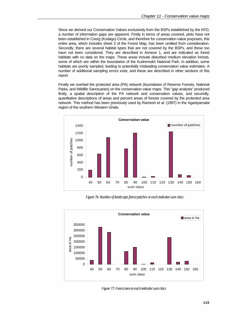
Chapter 11 - Conservation value maps
115
Since we derived our Conservation Values exclusively from the BSPs established by the KFD, a number of information gaps are apparent. Firstly in terms of areas covered, plots have not been established in Coorg (Kodagu) Circle, and therefore for conservation value purposes, this entire area, which includes sheet 3 of the Forest Map, has been omitted from consideration. Secondly, there are several habitat types that are not covered by the BSPs, and these too have not been considered. They are described in Annexe 1, and are indicated as forest habitats with no data on the maps. These areas include disturbed medium elevation forests, some of which are within the boundaries of the Kudremukh National Park. In addition, some habitats are poorly sampled, leading to potentially misleading conservation value estimates. A number of additional sampling errors exist, and these are described in other sections of this report.
Finally we overlaid the protected area (PA) network (boundaries of Reserve Forests, National Parks, and Wildlife Sanctuaries) on the conservation value maps. This “gap analysis” produced firstly, a spatial description of the PA network and conservation values, and secondly, quantitative descriptions of areas and percent areas of forests covered by the protected area network. This method has been previously used by Ramesh et al. (1997) in the Agastyamalai region of the southern Western Ghats.
Conservation value
0
200
400
600
800
1000
1200
1400
40 50 60 70 80 90 100 110 120 130 140 150 160sum class
num
ber o
f pat
ches
number of patches
Figure 76: Number of landscape forest patches in each indicator sum class
Conservation value
050000
100000150000200000250000300000350000
40 50 60 70 80 90 100 110 120 130 140 150 160sum class
area
in h
a
area in ha
Figure 77: Forest area in each indicator sum class
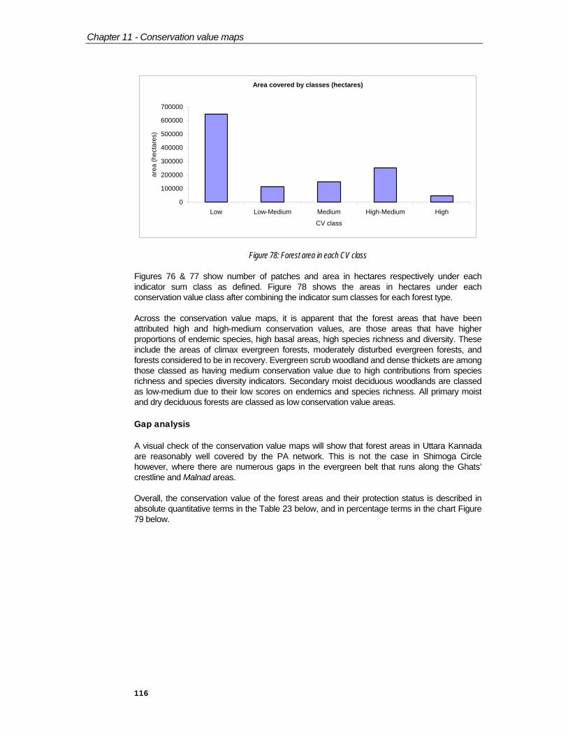
Chapter 11 - Conservation value maps
116
Area covered by classes (hectares)
0
100000
200000
300000
400000
500000
600000
700000
Low Low-Medium Medium High-Medium High
CV class
area
(hec
tare
s)
Figure 78: Forest area in each CV class
Figures 76 & 77 show number of patches and area in hectares respectively under each indicator sum class as defined. Figure 78 shows the areas in hectares under each conservation value class after combining the indicator sum classes for each forest type.
Across the conservation value maps, it is apparent that the forest areas that have been attributed high and high-medium conservation values, are those areas that have higher proportions of endemic species, high basal areas, high species richness and diversity. These include the areas of climax evergreen forests, moderately disturbed evergreen forests, and forests considered to be in recovery. Evergreen scrub woodland and dense thickets are among those classed as having medium conservation value due to high contributions from species richness and species diversity indicators. Secondary moist deciduous woodlands are classed as low-medium due to their low scores on endemics and species richness. All primary moist and dry deciduous forests are classed as low conservation value areas.
Gap analysis
A visual check of the conservation value maps will show that forest areas in Uttara Kannada are reasonably well covered by the PA network. This is not the case in Shimoga Circle however, where there are numerous gaps in the evergreen belt that runs along the Ghats’ crestline and Malnad areas.
Overall, the conservation value of the forest areas and their protection status is described in absolute quantitative terms in the Table 23 below, and in percentage terms in the chart Figure 79 below.

Chapter 11 - Conservation value maps
117
Table 23: Areas (in hectares) of conservation value classes under different protection regimes
Cons. Val. No protection ReserveForest (rf)
WildlifeSanctuary
(wls)
NationalPark(np)
Total
Low 4,568.75 4,255.12 744.00 1.56 9,569.43Low-Medium 801.12 1,493.19 200.57 136.10 2,630.99Medium 1,138.56 323.22 55.44 22.04 1,539.26High-Medium 1,478.67 2,565.33 377.49 427.81 4,849.31High 38.73 347.50 199.71 0.00 585.93
Proportion of areas under protection
0%10%20%30%40%50%60%70%80%90%
100%
1 2 3 4 5Conservation value class
Perc
ent a
rea np
wlsrfno protect
Figure 79: Protection status according to conservation value class
It is apparent that 93% of the High CV. (class 5) areas are under some form of protection. The other 7% are to be found outside the PA network. Most critically, thirty percent of forest areas classified as having high-medium conservation value (class 4 areas) are outside state protection. These areas generally surround the core areas of dense climax forests and areas of high endemicity along the crestline. They may be considered as important buffer areas, serving to modulate anthropogenic impact on the core. Furthermore, they are largely in a more fragmented condition and include areas such as Kan forests, which are unique ecosystems highly threatened by surrounding anthropogenic land cover types. Currently 58.48% of a total of 8,412 ha of this type is outside state protection. These areas may be expected to further deteriorate or disappear if not afforded protection.
It is worth emphasising that our conservation values were derived from tree biodiversity indicators that were for the most part inadvertently biased against such formations as deciduous forests. Although these areas scored highly in terms of basal area, they scored very low in terms of endemics, and species diversity. Ultimately, this may be misleading and certainly cannot be taken at its face value. It is well known that primary moist and dry deciduous forests in the study area are a vital habitat for large mammals, and the (continued) preservation of these habitats in large, contiguous expanses is of crucial importance. It is recommended that further work be carried out to expand and diversify the indicators used in deriving conservation values to include such categories as diversity of fauna (insects, birds, and large mammals), and presence of species with high economic and use values such as timber hardwood species and bamboo.
118
Conclusions and Recommendations A summary of the main findings, some suggestions towards the management of forests, and further work.
The main findings
Biodiversity assessment
A number of significant outcomes have emerged from the study. From the tree biodiversity assessment track, we can derive the following;
Due to a longer dry period, the Karnataka part of the Western Ghats (KWG) is relatively less diverse in terms of species richness when compared to the southern region of the Western Ghats. Despite the low diversity, Poeciloneuron forests, Memecylon forests, Corypha umbraculifera facies, Myristica swamps, and Kan forests, as well as pockets of Saraca asoca and Mamea suriga are unique formations in the study area.
The KWG represents 171 (49%) of the 352 endemic tree species recorded in the Western Ghats. Of these 30% (51 endemic species) are recorded in the BSPs. Species such as Garcinia indica, Mamea suriga, Hopea canarensis, Hopea jacobi, Bauhinia foveolata, are endemic to KWG.
At the regional level, the major types of vegetation are basically determined by bioclimate. However, the different intensity and mode of anthropogenic pressures have modified the vegetation into various degrees of degradation stages. These changes are reflected in the spatial and floristic structural parameters.
In the potential zone of evergreen forests, the changes are more apparent in the ecological and phenological characteristics of the species composition. Although the total species richness and diversity vary less among the different degradation stages of the evergreen forest, the proportion of primary evergreen species and endemics decreases with increasing degradation. On the other hand, secondary evergreen and deciduous species show an increase. The forests with moderate disturbance are in a state of recovery with good regeneration.
In the deciduous forest types, since the species are mostly those with wider ecological amplitude, degradation may not affect the overall species composition. However, changes are manifested in the basal area, which shows a sharp decline with increasing degradation.
The evergreen forests are rich in resources (timber, NTFPs, and medicinal plants) compared to other types. However, with the disturbance there is a drastic reduction in these resource species, which may be more attributed to the mode of harvesting as seen in the examples of Hopea ponga, Vateria indica and Garcinia indica.
Chapter
12
Chapter 12 – Conclusions and recommendations
119
Landscape ecology
The studies of landscape ecology showed that forests have been lost in the study area at the annual rate of 0.63%. This, however, does not consider the fact that rates of loss have been higher in some districts, and less in others.
Forest loss has been mitigated in areas of “Reserve Forest” under State protection. This also needs to be qualified. Many Reserve Forests are located in steep, inaccessible terrain that does not favour alternative use. Therefore, it may be that factors other than state protection are moderating forest loss.
Forest patches that were already degraded or fragmented lost relatively more area than dense or undisturbed forest. This indicates that forest loss in the study area for the most part may be an incremental process that proceeds first through degradation and fragmentation, and then to loss and conversion to other types of land-cover.
The exception to the above is in cases where forests have been cleared outright to make way for reservoirs, dams, mining projects and associated developmental activity. Over the last twenty years large reservoirs have come up in the study area. Dams continue to be built in the region, in many cases, such as in the Sharavati river valley this entails large losses of biodiverse forest.
Most critically, it has been shown that the phenomenal and unchecked increase in coffee cultivation in the districts of Kodagu, Hassan and Chickmagalur has destroyed and continues to seriously threaten the biodiversity of forests in the study area.
The degradation of betta lands are an important source of forest area loss in Uttara Kannada. Landscape analyses carried out within this study have supported ground observations on the effect and extent of arecanut cultivation on surrounding forest structure.
Gaps in the protected area network
There are numerous gaps in the PA network. Our studies have shown that there are large areas of biologically diverse forest that are not under conventional forms of protection. Notably, 30% of areas we have designated as having high-medium conservation value are outside State protection. Many of these areas are within the Shimoga circle. Figures from Uttara Kannada circle show that most areas of high-medium conservation value forest are within the protected area network. High-medium conservation value areas outside the PA network include unique ecosystems such as ‘Kan’ forests, and forests that were moderately disturbed in the past, and may be considered “in recovery” at present following the ban on green felling and timber extraction.
Suggestions on management
As an initial step towards the delineation of zone 1 (ecologically important areas), we suggest that those areas we have designated as having high and high-medium conservation value be incorporated into this zone. Within this, there will be a core of high conservation value areas that are to be monitored and managed with conservation of biodiversity, water, and soil as the highest priorities. Areas under zone 1 may be subsequently enlarged to include dense primary deciduous forests as an important habitat for wildlife.
Medium conservation value areas as defined by this study may constitute one of the other zones under the WGFP objectives. These areas would include fragmented and relatively degraded patches of forest which still contain high species richness and diversity. These areas may be managed carefully for regeneration, and eventually for mixed commercial production.

Chapter 12 – Conclusions and recommendations
120
The remaining areas may be designated according to Forest Department priorities in consultation with local people. Fuelwood, construction timber, fodder, green manure, and other NTFP needs of people have to be met from as many alternative sources as possible in order to reduce pressures on remaining areas of dense forest. Co-operative management must be emphasised wherever possible. From empirical studies and from the historical literature, it appears that local populations are largely undeterred by punitive measures, and will seek to satisfy local needs regardless.
Although there is presently a ban on green felling in place, there as still a number of species, including endemics, which are endangered due to over-exploitation of their non-timber product. For example, Garcinia indica and Myristica spp. are harvested for their fruit. This has led to enormous quantities being removed out of commercial pressure, and regeneration is now almost non-existent in certain areas. This sort of overuse must be carefully monitored and guidelines put in place.
Suggestions on further work
The areas of essential further work can be described broadly as follows;
The permanent biodiversity monitoring plots are a valuable source of data on extent of disturbance, species diversity and regeneration, among other factors. They serve to gauge the state of the forest, to provide baseline data, and to monitor ecosystem changes. Currently there are too many gaps in their coverage. It is imperative that more plots be established, particularly in forest areas that are not presently covered such as in Coorg circle, as well as the numerous habitat types, such as medium and high elevation evergreen forests for which little or no usable data exists. Thus there is a need to consolidate and extend the network of plots so as to create a “permanent observatory” of the biodiversity of the Karnataka Western Ghats and to assist the refining of management practices.
It is necessary to carry out studies or to incorporate existing data that would enable the expansion of conservation priority indicators to include parameters of wider ecological significance. For example, the importance of certain habitat types to large fauna, the presence of species of economic, medicinal or other use value, unique habitat areas, areas of cultural importance, among others. The use of multiple biological and non-biological criteria in setting conservation priorities has also been emphasised elsewhere (Johnson, 1995). The use of Geographical Information Systems and spatial management systems would enable the integration and consolidation of data of a range of hierarchical levels, and from diverse sources. Spatial databases have the potential to be disseminated and used widely on desktop systems, thus enabling decentralised decision making and management based on readily available, up to date spatial information.
With the available data on changes to biodiversity indicators with varying degrees of disturbance, it may be possible to construct models that simulate disturbance regimes and their impacts upon the forest physiognomy and species composition. Modelling the effect of various types of activity, particularly on sensitive areas, would allow an informed assessment of potential environmental impact and a comparison of costs and benefits, which also takes into account the losses of biological diversity.
There is a need to carry out or incorporate data on finer scale studies of forest and landscape change linked to social and economic studies of forest use and management. These would shed light on some of the proximate and underlying causes of deforestation and loss of biodiversity. Wherever feasible, this may be extended to cover larger areas, and would lead to more effective regional natural resource management.

Chapter 12 – Conclusions and recommendations
121
New approaches that are holistic, integrative, and involve multiple agents would require a degree of coordination and cooperation between institutions. It would be useful for the State Forest Department to assume a leading role in this, and to invite participating institutions to share their findings and to propose resource management alternatives based on empirical studies. There also needs to be better coordination among government agencies and research institutions. For example, between the state Forest Departments and the Revenue Department, who between them administer vast tracts of land in India.
The links between Research & Development and Extension services need to be better defined and better implemented. The Joint Forest Planning and Management (JFPM) experiment, according to some reports (Outreach, 1998), has been a good attempt overall by the Forest Department to enter into a participatory mode. These projects will need to be continued, extended to cover a broader geographical area, and closely monitored for their impact on forests and on the livelihood security of the participants.
Most critically perhaps, we reiterate here that biodiversity conservation must be integrated with national planning and economic / infrastructural priorities. Article 6 of the Convention on Biological Diversity calls upon signatory countries to approach biodiversity planning in a comprehensive manner (Johnson, 1995). Biological diversity must be assigned a high priority based upon long-term planning and studies of human-ecosystem relationships.

Bibliography
Ayyappan, N. & Parthasarathy, N. (1999) Biodiversity inventory of trees in a large-scale permanent plot of tropical evergreen forest at Varagalaiar, Anamalais, Western Ghats, India, Biodiversity and Conservation 8: 1533-1554.
Bourdillon, T.F. (1908) Forest trees of Travancore, The Travancore Government Press, Trivandrum: pp 456.
Bourgeon, G. & Pascal, J.P. (1986) Influences des heritages morphopedologiques dans la repartition des formations forestieres: region de Sorab-Siddapur (Inde du sud). Bois et Forets des Tropiques 214: 3-21.
Caius, J.F. (1986) The Medicinal and Poisonous Plants of India, Scientific Publishers, Jodhpur, India: pp 528.
Chandrabose, M. & Nair, N.C. (1987) Flora of Coimbatore, Bishan Singh Mahendra Pal Singh, Dehra Durn: pp 398.
Chandrasekara, U.M. & Ramakrishnan, P.S. (1994) J. Trop. Ecol., 10: 323-354.
Daniels, R.J.R., M. Gadgil & Joshi, N.V. (1995) Impact of human extraction on tropical humid forests in the Western Ghats in Uttara Kannada, South India, Journal of Applied Ecology 32: 866-874.
Derouet L. (1994) Étude de la variabilité structurale de huit populations d’arbres en forêt tropicale humide (Forêt d’Uppangala, Inde). Mémoire de DEA Analyse et Modélisation des Systèmes Biologiques, Université Claude Bernard (Lyon I), CNRS-URA 2055, 30 pp.+ann.
Elouard, C., Pascal, J.P., Ramesh, B.R., Houllier, F., Durand, M., Aravajy, S., Moravie, M.A., Gimaret-Carpentier, C. (1997) Monitoring the dynamics and moisture of a dense moist evergreen forest in the Western Ghats (Kodagu District, Karnataka, India). J. of Tropical Ecology. 38 (2): 193-214.
Faber-Langendoen, D. & Gentry, A.H. (1991) The structure and diversity of rain forests at Bajo Calima. Choco Region, Western Colombia, Biotropica 23: 2-11.
Ganesh, T., Ganesan, R., Soubadra Devy, Davidar, P. & Bawa, K.S. (1996) Assessment of plant biodiversity at a mid-elevation evergreen forest of Kalakad-Mundanthurai Tiger Reserve, Western Ghats, India. Current Science 71: 379-392.
Gentry, A.H. (1988b) Species richness of upper Amazonia In: Proc. Nat. Acad. Sci. U.S.A. 85: 156-159.
Gentry, A.H. (1990) Floristic similarities and differences between southern Central America and Upper and Central Amazonia. In: Four neotropical rain forests (Edited by A.H. Genry),Yale University Press, New Haven: pp. 141-157.
Gentry, A.H., & Terborgh (1990) Composition and dynamics of the Cocha Cashu “mature“ floodplain forest. In Four neotropical rain forests (Edited by A.H. Genry) Yale University Press, New Haven: pp. 542-564.
Ghate, U., Joshi, N.V. & Gadgil, M. (1998) On the patterns of tree diversity in the Western Ghats of India. Current Science 75: 594-603.

Jain, S.K. (1981) Glimpses of Indian Ethnobotany, Oxford and IBH Publishing Co. New Delhi: pp 365.
Johnson, N. (1995) Biodiversity in the Balance: Approaches to Setting Geographic Conservation Priorities. World Resource Institute 1709 Washington D.C. 20006.
Keshava Murthy, K.R. & Yoganarasimhan, S.N. (1990) Flora of Coorg, Vimsat Publishers, Bangalore: pp 711.
Kochummen, K.M., Lefrankie, J.V. & Manokaran, N. (1990) Floristic composition of Pasoh Forest Reserve, a lowland rain forest in Peninsular Malaysia In: J. Trop. For. Sci. 3: 1-13.
Lieberman, M., Lieberman, D., Hartshorn, G.S. & Peralta, R. (1985) Small-scale altitudinal variation in lowland wet tropical forest vegetation In: J. Ecol. 73: 505-516.
Loffeier, M.E. (1989) Sylviculture et sylvigenese en foret sempervirente du Coorg (sud-ouest de l'Inde). Inst. fr. Pondichéry, trav. sec. sci. tech. Tome 26: p. 211.
Magurran, A. (1988) Ecological Diversity and its Measurement. Princeton University Press, Princeton: pp 179.
Nadkarni, M.V., Pasha, S.A. & Prabhakar, L.S. (1989) The Political Economy of Forest Use and Management, Sage Publications, New Delhi: pp 182.
Nayar, M.P. (1996) Hot spots of Endemic plants of India, Nepal and Bhutan. Tropical Botanical Garden and Research Institute, Tiruvananthapuram: 252p.
Outreach (1998). Social Impact Assessment of JFPM of Western Ghats. Report submitted DFIP.
Parthasarathy, N. (1999) Tree diversity and distribution in undisturbed and human-impacted sites of tropical wet evergreen forest in southern Western Ghats, India, Biodiversity and Conservation 8: 1365-1381.
Pascal J.-P., & Pélissier R. (1996) Structure and floristic composition of a tropical evergreen forest in southwest India. Journal of Tropical Ecology, 12 (2): 191-214.
Pascal, J.P. & Ramesh, B.R. (1986) A field key to the trees and lianas of the evergreen forests of the Western Ghats, India. Institut Français de Pondichéry, Publications du départment d'écologie.
Pascal, J.P. (1982a) Bioclimates of the Western Ghats at 1/250,000 (2 sheets). Inst. fr. Pondichéry, trav. sec.sci. tech. Hors série 17.
Pascal, J.P. (1986) Explanatory booklet on the Forest Map of South India - Sheets: Belgaum-Dharwar-Panaji; Shimoga; Mercara-Mysore. Published by the Karnataka Forest Department and the French Institute of Pondicherry. Inst. fr. Pondichéry, trav. sec. sci. tech. Hors série 18.
Pascal, J.P. (1988) Wet evergreen forests of the Western Ghats of India. Inst. fr. Pondichéry, trav. sec. sci. tech. Tome 20 bis. p. 345.
Pascal, J.P., Ramesh, B.R. & Bourgeon, G. (1988) The ”Kan Forests” of the Karnataka plateau (India): Structure and Floristic composition, trends in the changes due to their exploitation, Tropical Ecology 29(2): 9-23.
Pelissier, R. (1997) Hétérogénéite spatiale et dynamique d’une foret humide dans les Ghats occidentaux de l’Inde. 37: p 148. Publications du département d'écologie, Institut Français de Pondichéry, Pondicherry.

Phillips, O.L., Hall, P., Gentry, A.H., Sawyer, S.A. & Vasquez, R. (1994) Dynamics and species richness of tropical rain forests In: Proc. Natl. Acad. U.S.A. 91: 2805-2809.
Proctor, J., Anderson, J.M., Chai, P. & Vallack, H.W. (1983) Ecological studies in four contrasting lowland rain forests in Gunung Mulu National Park, Sarawak, J. Ecol. 71: 237-260.
Rama Rao, R. & Sahib, M. (1914) Flowering plants of Travancore, The Government Press, Trivandrum: pp 496.
Ramesh, B.R. & Pascal, J.P. (Geomatics by Nouguier, C.) (1997) Atlas of Endemics of the Western Ghats (India). Distribution of tree species in the evergreen and semi-evergreen forests. Institut Francais de Pondicherry, Publications du departement d’ecologie 38.
Ramesh, B.R., De Franceschi, D. & Pascal, J.P. (1997) Forest Map of South India - sheet: Tiruvananthapuram-Tirunelveli, Hors série 22a, Published by the Kerala and Tamil Nadu Forest Departments and the French Institute of Pondicherry. Institut Français de Pondichéry, Publications du départment d'écologie.
Ramesh, B.R., Menon, S. & Bawa, K.S. (1997) A Vegetation Based Approach to Biodiversity Gap Analysis in the Agastyamalai Region, Western Ghats, India. Ambio Vol. 26(8): 529-536.
Ramesh, B.R., Pascal, J.P. & De Franceschi, D. (1996) Distribution of Dipterocarpaceae in the Western Ghats, South India. In Proceedings of fifth round-table conference on Dipterocarps, (Ed. Appanah, S. & Khoo, K.C.), Forest Research Institute Malaysia, Kuala Lumpur : 47-59.
Subramanian, K.N. (1995) Flora of Thenmala, International Book Distributors, Dehra Dun: pp 516.
Subramanian, K.N., Venkatasubramanian, N. & Nallaswamy, V.K. (1987) Flora of Palghat, Bishen Singh Mahendra Pal Singh, Dehra Durn, India: pp 149.
Sukumar, R., Dattaraja, H.S., Suresh, H.S., Radhakrishnan, J.V.,Vasudeva, R., Nirmala, S. & Joshi, N.V. (1992) Long-term monitoring of vegetation in a tropical deciduous forest in Madumalai, Southern India. Current Science 62: 608-616.
Swamy, R.H. & Proctor, J. (1994) Rain forests and their soils in the Sringeri area of the Indian Western Ghats. Global Ecology and Biogeography Letters 4: 140-154.
Thioulouse, J., Chessel, D., Doledec, S. & Olivier, J.M. (1995) Analyse des Donnes Ecologique (ADE-4, Base version12) for Windows 95.
Uhl, C., & Murphy, P.G. (1981) Composition, structure, and regeneration of a terra firme forest in the Amazon Basin of Venezuela, Top. Ecol. 22: 219-237.
Valencia, R., Balslev, H.G., Paz Y, & Mino C. (1994) High Tree alpha-diversity in Amazonian Ecuador In: Biodiv. Conserv. 3: 21-28.
Wright, D. D., Jessen, J. H., Burke, P. and Gomez d Silva Garza, H. (1997). Tree and liana enumeration and diversity on a 1-ha plot in Papua New Guinea. Biotropica 29(3): 250-260.

Annexe 1
Annexe 1
A table describing forest classification on sheets 1 to 3 of the Forest Map (Forest habitat types not represented by BSPs are shaded grey)
group1 mainGroup SubGroup Physiognomy elevation Type wet evergreen climax and related forests
Wet evergreen and semi - evergreen climax forests and degradation stages
Wet evergreen or semi - evergreen climax and potentially related forests
Disturbed to semi-evergreen
Low elevation
Dipterocarpus indicus - Humboldtia brunonis - Poeciloneuron indicum type
wet evergreen climax and related forests
Wet evergreen and semi - evergreen climax forests and degradation stages
Wet evergreen or semi - evergreen climax and potentially related forests
Dense evergreen
Low elevation
Dipterocarpus indicus - Humboldtia brunonis - Poeciloneuron indicum type
wet evergreen climax and related forests
Wet evergreen and semi - evergreen climax forests and degradation stages
Wet evergreen or semi - evergreen climax and potentially related forests
Disturbed to semi-evergreen
Low elevation
Poeciloneuron indicum facies of Dipterocarpus indicus - Kingiodendron pinnatum - Humboldtia brunonis type
wet evergreen climax and related forests
Wet evergreen and semi - evergreen climax forests and degradation stages
Wet evergreen or semi - evergreen climax and potentially related forests
Dense evergreen
Low elevation
Poeciloneuron indicum facies of Dipterocarpus indicus - Kingiodendron pinnatum - Humboldtia brunonis type
wet evergreen climax and related forests
Wet evergreen and semi - evergreen climax forests and degradation stages
Wet evergreen or semi - evergreen climax and potentially related forests
Disturbed to semi-evergreen
Low elevation
Dipterocarpus indicus - Kingiodendron pinnatum - Humboldtia brunonis type
wet evergreen climax and related forests
Wet evergreen and semi - evergreen climax forests and degradation stages
Wet evergreen or semi - evergreen climax and potentially related forests
Dense evergreen
Low elevation
Dipterocarpus indicus - Kingiodendron pinnatum - Humboldtia brunonis type
wet evergreen climax and related forests
Wet evergreen and semi - evergreen climax forests and degradation stages
Wet evergreen or semi - evergreen climax and potentially related forests
Kan Low elevation
Diospyros spp. - Dysoxylum malabaricum - Persea macrantha "kan" forest type
wet evergreen climax and related forests
Wet evergreen and semi - evergreen climax forests and degradation stages
Wet evergreen or semi - evergreen climax and potentially related forests
Disturbed to semi-evergreen
Low elevation
Poeciloneuron indicum facies of Dipterocarpus indicus - Persea macrantha type
wet evergreen climax and related forests
Wet evergreen and semi - evergreen climax forests and degradation stages
Wet evergreen or semi - evergreen climax and potentially related forests
Disturbed to semi-evergreen
Low elevation
Dipterocarpus indicus - persea macrantha type
wet evergreen climax and related forests
Wet evergreen and semi - evergreen climax forests and degradation stages
Wet evergreen or semi - evergreen climax and potentially related forests
Disturbed to semi-evergreen
Low elevation
Persea macrantha - Diospyros spp. - Holigarna spp. type
wet evergreen climax and related forests
Wet evergreen and semi - evergreen climax forests and degradation stages
Wet evergreen or semi - evergreen climax and potentially related forests
Dense evergreen
Low elevation
Dipterocarpus indicus - Diospyros candolleana - Diospyros oocarpa type
wet evergreen climax and related forests
Wet evergreen and semi - evergreen climax forests and degradation stages
Wet evergreen or semi - evergreen climax and potentially related forests
Dense evergreen
Low elevation
Poeciloneuron indicum facies of Dipterocarpus indicus - Diospyros candolleana - Diospyros oocarpa type

Annexe 1
wet evergreen climax and related forests
Wet evergreen and semi - evergreen climax forests and degradation stages
Wet evergreen or semi - evergreen climax and potentially related forests
Disturbed to semi-evergreen
Low elevation
Dipterocarpus indicus - Diospyros candolleana - Diospyros oocarpa type
wet evergreen climax and related forests
Wet evergreen and semi - evergreen climax forests and degradation stages
Wet evergreen or semi - evergreen climax and potentially related forests
Disturbed to semi-evergreen
Low elevation
Poeciloneuron indicum facies of Dipterocarpus indicus - Diospyros candolleana - Diospyros oocarpa type
wet evergreen climax and related forests
Wet evergreen and semi - evergreen climax forests and degradation stages
Wet evergreen or semi - evergreen climax and potentially related forests
Dense evergreen
Medium elevation
Cullenia exarillata - Mesua ferrea - palaquium ellipticum
wet evergreen climax and related forests
Wet evergreen and semi - evergreen climax forests and degradation stages
Wet evergreen or semi - evergreen climax and potentially related forests
Disturbed to semi-evergreen
Medium elevation
Memecylon umbellatum - Syzygium cumini - Actinodaphne anguistifolia type
wet evergreen climax and related forests
Wet evergreen and semi - evergreen climax forests and degradation stages
Wet evergreen or semi - evergreen climax and potentially related forests
Disturbed to semi-evergreen
High elevation
Schefflera spp. - Gordonia obtusa - Meliosma arnottiana type
wet evergreen climax and related forests
Wet evergreen and semi - evergreen climax forests and degradation stages
Wet evergreen or semi - evergreen climax and potentially related forests
Dense evergreen
Medium elevation
Mesua ferrea - Palaquium ellipticum type
wet evergreen climax and related forests
Wet evergreen and semi - evergreen climax forests and degradation stages
Wet evergreen or semi - evergreen climax and potentially related forests
Disturbed to semi-evergreen
Medium elevation
Mesua ferrea - Palaquium ellipticum type
wet evergreen climax and related forests
Wet evergreen and semi - evergreen climax forests and degradation stages
Wet evergreen or semi - evergreen climax and potentially related forests
Dense evergreen
Medium elevation
Palaquium ellipticum - poeciloneuron indicum - Hopea canalensis type
wet evergreen climax and related forests
Wet evergreen and semi - evergreen climax forests and degradation stages
Wet evergreen or semi - evergreen climax and potentially related forests
Dense evergreen
High elevation
Schefflera spp. - Gordonia obtusa - Meliosma arnottiana type
wet evergreen climax and related forests
Wet evergreen and semi - evergreen climax forests and degradation stages
Wet evergreen or semi - evergreen climax and potentially related forests
Disturbed to semi-evergreen
Medium elevation
Palaquium ellipticum - poeciloneuron indicum - Hopea ponga type
moist deciduous forests
Deciduous climax forests and degradations
Moist deciduous forests
Scrub woodland to thicket
Lagestroemia microcarpa - Tectona grandis - Dillenia pentagyna type
moist deciduous forests
Deciduous climax forests and degradations
Moist deciduous forests
Woodland to savanna woodland
Lagestroemia microcarpa - Tectona grandis - Dillenia pentagyna type
moist deciduous forests
Deciduous climax forests and degradations
Moist deciduous forests
Dense Lagestroemia microcarpa - Tectona grandis - Dillenia pentagyna type
moist deciduous forests
Deciduous climax forests and degradations
Moist deciduous forests
Discontinuous thicket to low scattered shrubs
Lagestroemia microcarpa - Tectona grandis - Dillenia pentagyna type
dry deciduous forests
Deciduous climax forests and degradations
Dry deciduous forests
Scrub woodland to thicket
Anogeissus latifolia - Tectona grandis - Terminalia tomentosa type
dry deciduous forests
Deciduous climax forests and degradations
Dry deciduous forests
Tree savanna Anogeissus latifolia - Tectona grandis - Terminalia tomentosa type
dry deciduous forests
Deciduous climax forests and degradations
Dry deciduous forests
Woodland to savanna woodland
Anogeissus latifolia - Tectona grandis - Terminalia tomentosa type
dry deciduous forests
Deciduous climax forests and degradations
Dry deciduous forests
Dense Anogeissus latifolia - Tectona grandis - Terminalia tomentosa type
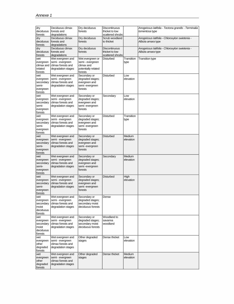
Annexe 1
dry deciduous forests
Deciduous climax forests and degradations
Dry deciduous forests
Discontinuous thicket to low scattered shrubs
Anogeissus latifolia - Tectona grandis - Terminalia tomentosa type
dry deciduous forests
Deciduous climax forests and degradations
Dry deciduous forests
Scrub woodland to thicket
Anogeissus latifolia - Chloroxylon swietenia - Albizia amara type
dry deciduous forests
Deciduous climax forests and degradations
Dry deciduous forests
Discontinuous thicket to low scattered shrubs
Anogeissus latifolia - Chloroxylon swietenia - Albizia amara type
wet evergreen climax and related forests
Wet evergreen and semi - evergreen climax forests and degradation stages
Wet evergreen or semi - evergreen climax and potentially related forests
Disturbed Transition type
Transition type
wet evergreen secondary semi-evergreen forests
Wet evergreen and semi - evergreen climax forests and degradation stages
Secondary or degraded stages; evergreen and semi -evergreen forests
Disturbed Low elevation
wet evergreen secondary semi-evergreen forests
Wet evergreen and semi - evergreen climax forests and degradation stages
Secondary or degraded stages; evergreen and semi -evergreen forests
Secondary Low elevation
wet evergreen secondary semi-evergreen forests
Wet evergreen and semi - evergreen climax forests and degradation stages
Secondary or degraded stages; evergreen and semi -evergreen forests
Disturbed Transition type
wet evergreen secondary semi-evergreen forests
Wet evergreen and semi - evergreen climax forests and degradation stages
Secondary or degraded stages; evergreen and semi -evergreen forests
Disturbed Medium elevation
wet evergreen secondary semi-evergreen forests
Wet evergreen and semi - evergreen climax forests and degradation stages
Secondary or degraded stages; evergreen and semi -evergreen forests
Secondary Medium elevation
wet evergreen secondary semi-evergreen forests
Wet evergreen and semi - evergreen climax forests and degradation stages
Secondary or degraded stages; evergreen and semi -evergreen forests
Disturbed High elevation
wet evergreen secondary moist deciduous forests
Wet evergreen and semi - evergreen climax forests and degradation stages
Secondary or degraded stages; secondary moist deciduous forests
Dense
wet evergreen secondary moist deciduous forests
Wet evergreen and semi - evergreen climax forests and degradation stages
Secondary or degraded stages; secondary moist deciduous forests
Woodland to savanna woodland
wet evergreen other degraded forests
Wet evergreen and semi - evergreen climax forests and degradation stages
Other degraded stages
Dense thicket Low elevation
wet evergreen other degraded forests
Wet evergreen and semi - evergreen climax forests and degradation stages
Other degraded stages
Dense thicket Medium elevation
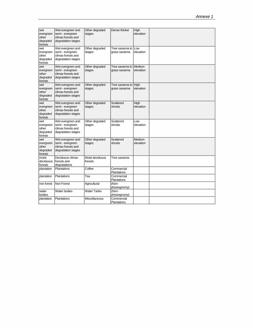
Annexe 1
wet evergreen other degraded forests
Wet evergreen and semi - evergreen climax forests and degradation stages
Other degraded stages
Dense thicket High elevation
wet evergreen other degraded forests
Wet evergreen and semi - evergreen climax forests and degradation stages
Other degraded stages
Tree savanna to grass savanna
Low elevation
wet evergreen other degraded forests
Wet evergreen and semi - evergreen climax forests and degradation stages
Other degraded stages
Tree savanna to grass savanna
Medium elevation
wet evergreen other degraded forests
Wet evergreen and semi - evergreen climax forests and degradation stages
Other degraded stages
Tree savanna to grass savanna
High elevation
wet evergreen other degraded forests
Wet evergreen and semi - evergreen climax forests and degradation stages
Other degraded stages
Scattered shrubs
High elevation
wet evergreen other degraded forests
Wet evergreen and semi - evergreen climax forests and degradation stages
Other degraded stages
Scattered shrubs
Low elevation
wet evergreen other degraded forests
Wet evergreen and semi - evergreen climax forests and degradation stages
Other degraded stages
Scattered shrubs
Medium elevation
moist deciduous forests
Deciduous climax forests and degradations
Moist deciduous forests
Tree savanna
plantation Plantations Coffee Commercial Plantations
plantation Plantations Tea Commercial Plantations
non forest Non Forest Agricultural (Non-physiognomy)
water bodies
Water bodies Water Tanks (Non-physiognomy)
plantation Plantations Miscellaneous Commercial Plantations
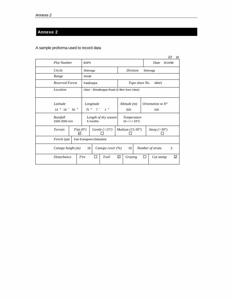
Annexe 2
Annexe 2
A sample proforma used to record data ID 36 Plot Number BSP5 Date 9/14/98
Circle Shimoga Division Shimoga Range Sorab Reserved Forest Karjikoppa Topo sheet No. 48N/3 Location Ulavi - Shiralkoppa Road (0.9km from Ulavi)
Latitude Longitude Altitude (m) Orientation to N° 14 ° 16 ' 55 " 75 ° 7 ' 1 " 620 100
Rainfall Length of dry season Temperature 1500-2000 mm 6 months 16 < t < 23°C
Terrain Flat (0°) Gentle (<15°) Medium (15-30°) Steep (>30°) Forest type Kan Evergreen-Disturbed
Canopy height (m) 28 Canopy cover (%) 55 Number of strata 3
Disturbance Fire Trail Grazing Cut stump
Annexe 3
Annexe 3
Biodiversity Sampling plots and Forest types
ID Plot Circle Division Forest Type 1 PSPD1 Uttara
Kannada Sirsi Secondary moist deciduous-Scrub woodland-Open
thickets 2 PSPD2 Uttara
Kannada Sirsi Secondary moist deciduous-Open thickets
3 PSPD3 Uttara Kannada
Sirsi Secondary moist deciduous-Woodland-Open thickets
4 PSPLD1 Uttara Kannada
Sirsi Secondary moist deciduous-Woodland-Dense thickets
5 PSPLD2 Uttara Kannada
Sirsi Kan Evergreen-Disturbed
6 PSPLD3 Uttara Kannada
Sirsi Wet Evergreen-Dense
7 PSPD1 Uttara Kannada
Yellapur Secondary moist deciduous-Woodland
8 PSPD2 Uttara Kannada
Yellapur Secondary moist deciduous-Woodland
9 PSPD3 Uttara Kannada
Yellapur Scrub woodland-Open thickets
10 PSPLD1 Uttara Kannada
Yellapur Semi-Evergreen-Dense
11 PSPLD2 Uttara Kannada
Yellapur Semi-Evergreen-Dense
12 PSPLD3 Uttara Kannada
Yellapur Semi-Evergreen-Dense
13 PSPD1 Uttara Kannada
Karwar Secondary moist deciduous-Woodland-Open thickets
14 PSPD2 Uttara Kannada
Karwar Secondary moist deciduous-Scrub woodland
15 PSPD3 Uttara Kannada
Karwar Semi-Evergreen-Disturbed
16 PSPLD1 Uttara Kannada
Karwar Semi-Evergreen-Disturbed
17 PSPLD2 Uttara Kannada
Karwar Secondary moist deciduous-Scrub woodland
18 PSPLD3 Uttara Kannada
Karwar Semi-Evergreen-Disturbed
20 PSPD1 Uttara Kannada
Haliyal Primary moist deciduous-Woodland
21 PSPD2 Uttara Kannada
Haliyal Primary moist deciduous-Woodland
22 PSPD3 Uttara Kannada
Haliyal Primary moist deciduous-Woodland
23 PSPLD1 Uttara Kannada
Haliyal Primary moist deciduous-Disturbed-Woodland
24 PSPLD2 Uttara Kannada
Haliyal Primary moist deciduous-Disturbed-Woodland
25 PSPLD3 Uttara Kannada
Haliyal Primary moist deciduous-Disturbed-Woodland
26 PSPD1 Uttara Kannada
Honnavar Semi-Evergreen-Disturbed
27 PSPD2 Uttara Kannada
Honnavar Wet Evergreen-Disturbed
28 PSPD3 Uttara Kannada
Honnavar Wet Evergreen-Woodland-Open thickets

Annexe 3
29 PSPLD1 Uttara Kannada
Honnavar Wet Evergreen-Disturbed
30 PSPLD2 Uttara Kannada
Honnavar Semi-Evergreen-Disturbed
31 PSPLD3 Uttara Kannada
Honnavar Semi-Evergreen-Disturbed
33 BSP3 Shimoga Shimoga Primary moist deciduous-Disturbed-Woodland 34 BSP13 Shimoga Shimoga Secondary moist deciduous-Disturbed-Woodland 35 BSP12 Shimoga Shimoga Secondary moist deciduous-Disturbed-Woodland 36 BSP5 Shimoga Shimoga Kan Evergreen-Disturbed 37 BSP1 Shimoga Shimoga Kan Evergreen-Disturbed 41 BSP2 Shimoga Sagar Semi-Evergreen-Disturbed 42 BSP4 Shimoga Sagar Kan Evergreen-Disturbed 43 BSP6 Shimoga Sagar Secondary moist deciduous-Woodland 44 BSP15 Shimoga Sagar Primary moist deciduous-Woodland 45 BSP16 Shimoga Sagar Secondary moist deciduous-Disturbed-Woodland 46 BSP47 Shimoga Sagar Dry deciduous-Open thickets 47 BSP56 Shimoga Sagar Dry deciduous-Open thickets 48 BSP57 Shimoga Sagar Primary moist deciduous-Scrub woodland-Open
thickets 49 BSP58 Shimoga Sagar Primary moist deciduous-Open thickets 50 BSP59 Shimoga Sagar Primary moist deciduous-Dense thickets 51 BSP6 Shimoga Sagar Primary moist deciduous-Scrub woodland 52 BSP7 Shimoga Sagar Secondary moist deciduous-Open thickets 53 BSP8 Shimoga Sagar Secondary moist deciduous-Woodland-Open thickets 54 BSP1 Shimoga Shimoga Primary moist deciduous-Woodland 55 BSP11 Shimoga Shimoga Primary moist deciduous-Woodland 56 BSP14 Shimoga Sagar Dry deciduous-Open thickets 57 BSP17 Shimoga Sagar Secondary moist deciduous-Woodland-Open thickets 58 BSP2 Shimoga Sagar Secondary moist deciduous-Woodland-Dense thickets59 BSP22 Shimoga Shimoga Semi-Evergreen-Disturbed 60 BSP43 Shimoga Shimoga Dry deciduous-Woodland-Open thickets 61 BSP44 Shimoga Shimoga Dry deciduous-Open thickets 62 BSP45 Shimoga Shimoga Dry deciduous-Woodland 63 BSP46 Shimoga Shimoga Dry deciduous-Scrub woodland-Open thickets 64 BSP48 Shimoga Shimoga Secondary moist deciduous-Woodland-Open thickets 65 BSP27 Shimoga Kalasa Wild life Wet Evergreen-Dense 66 BSP28 Shimoga Kalasa Wild life Wet Evergreen-Dense 67 BSP29 Shimoga Kalasa Wild life Wet Evergreen-Disturbed 68 BSP3 Shimoga Kalasa Wild life Wet Evergreen-Disturbed-Tree savanna 69 BSP18 Shimoga Shimoga Wet Evergreen-Dense 70 BSP25 Shimoga Koppa Wet Evergreen-Dense 71 BSP19 Shimoga Shimoga Wet Evergreen-Disturbed-Tree savanna 72 BSP23 Shimoga Koppa Secondary Evergreen-Woodland-Savanna woodland-
Scrub woodland 73 BSP24 Shimoga Shimoga Wet Evergreen-Disturbed 74 BSP26 Shimoga Shimoga Wet Evergreen-Dense 75 BSP41 Shimoga Sagar Wet Evergreen-Disturbed 76 BSP42 Shimoga Sagar Wet Evergreen-Woodland 78 BSP49 Uttara
Kannada Sirsi Semi-Evergreen-Scrub woodland
79 BSP5 Uttara Kannada
Sirsi Secondary Evergreen-Dense
80 BSP53 Uttara Kannada
Sirsi Wet Evergreen-Dense
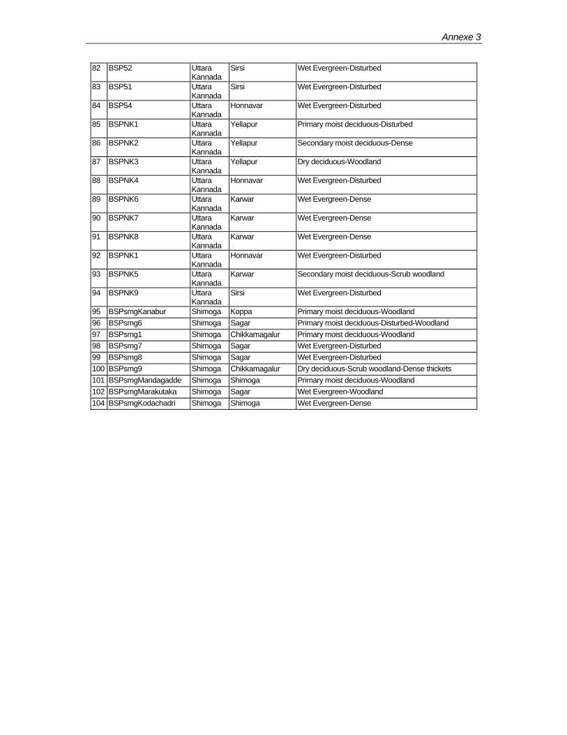
Annexe 3
82 BSP52 Uttara Kannada
Sirsi Wet Evergreen-Disturbed
83 BSP51 Uttara Kannada
Sirsi Wet Evergreen-Disturbed
84 BSP54 Uttara Kannada
Honnavar Wet Evergreen-Disturbed
85 BSPNK1 Uttara Kannada
Yellapur Primary moist deciduous-Disturbed
86 BSPNK2 Uttara Kannada
Yellapur Secondary moist deciduous-Dense
87 BSPNK3 Uttara Kannada
Yellapur Dry deciduous-Woodland
88 BSPNK4 Uttara Kannada
Honnavar Wet Evergreen-Disturbed
89 BSPNK6 Uttara Kannada
Karwar Wet Evergreen-Dense
90 BSPNK7 Uttara Kannada
Karwar Wet Evergreen-Dense
91 BSPNK8 Uttara Kannada
Karwar Wet Evergreen-Dense
92 BSPNK1 Uttara Kannada
Honnavar Wet Evergreen-Disturbed
93 BSPNK5 Uttara Kannada
Karwar Secondary moist deciduous-Scrub woodland
94 BSPNK9 Uttara Kannada
Sirsi Wet Evergreen-Disturbed
95 BSPsmgKanabur Shimoga Koppa Primary moist deciduous-Woodland 96 BSPsmg6 Shimoga Sagar Primary moist deciduous-Disturbed-Woodland 97 BSPsmg1 Shimoga Chikkamagalur Primary moist deciduous-Woodland 98 BSPsmg7 Shimoga Sagar Wet Evergreen-Disturbed 99 BSPsmg8 Shimoga Sagar Wet Evergreen-Disturbed 100 BSPsmg9 Shimoga Chikkamagalur Dry deciduous-Scrub woodland-Dense thickets 101 BSPsmgMandagadde Shimoga Shimoga Primary moist deciduous-Woodland 102 BSPsmgMarakutaka Shimoga Sagar Wet Evergreen-Woodland 104 BSPsmgKodachadri Shimoga Shimoga Wet Evergreen-Dense

Annexe 4
Annexe 4
List of species encountered in BSPs according to major forest types -Hab=Habitat Trees with potential height E=Emergent(>40 m) 1=Canopy (24-40 m) 2=2nd Strata (16-24 m) 3=3rd Strata (8-16 m) 4=4th Strata (<8 m) sh=shrub h=herb c=climber L=liana
-Phe=Phenology eg=Evergreen de=Deciduous
-Eco=Ecology s=Secondary Evergreen Species p=Primary Evergreen Speceis o=in openings Ex=Exotic
End=Endemic wg=Endemic to the Western Ghats
-WEG=Wet Evergreen -SEG=Semi Evergreen -KEG=Kan Evergreen -SGD=Secondary Moist Deciduous -PMD=Primary Moist Deciduous -DS=Dry Deciduous
Family Species Hab Phe Eco End WEG KEG SEG SMD PMD DD ACANTHACEAE Andrographis sp. h eg s X ACANTHACEAE Justisia sp. c eg s X X X X X ACANTHACEAE Nilgirianthus barbatus (Nees) Brem. 4 eg s X ACANTHACEAE Strobilanthes sp sh eg s X X X X ACANTHACEAE Thunbergia mysorensis (Wt.) Anders. L eg p wg X ADIANTACEAE Adiantum sp. h eg p X X X ALANGIACEAE Alangium salvifolium (L.f.) Wang var. hexapetalum L eg s X X X X X AMARYLLIDACEAE Curculigo orchiodes Gaertn. h eg s X X X X X X ANACARDIACEAE Buchanania lanzan Spreng. 4 de X X X X X ANACARDIACEAE Holigarna arnottiana J. Hk. 2 eg s wg X X X X ANACARDIACEAE Holigarna grahamii (Wt.) Kurz 1 eg s wg X X X X ANACARDIACEAE Holigarna nigra Bourd. 1 eg p wg X X ANACARDIACEAE Lannea coromandelica (Houtt.) Merr. 2 de s X X X X X X ANACARDIACEAE Mangifera indica L. 1 eg p X X X X X ANACARDIACEAE Nothopegia beddomei Gamble 3 eg p X ANACARDIACEAE Nothopegia racemosa (Dalz.) Ramam. 3 eg p X X X X ANACARDIACEAE Semecarpus anacardium L. 2 de X X X ANACARDIACEAE Spondias pinnata (L.f.) Kurz 1 eg p X X X X ANCISTROCLADACEAE Ancistrocladus heyneanus Wall. L eg p X X ANNONACEAE Annona reticulata L. 4 eg ex X ANNONACEAE Artabotrys zeylanicus J.Hk. & Thoms L eg p X ANNONACEAE Cyathocalyx zeylanicus Champ. ex J. Hk. & Th. 3 eg p X ANNONACEAE Desmos lawii (J. Hk. & Th.) Safford. L eg s X X X ANNONACEAE Goniothalamus cardiopetalus (Dalz.) J. Hk. &
Thoms. 4 eg p wg X
ANNONACEAE Meiogyne pannosa (Dalz.) Sinclair 3 eg p wg X ANNONACEAE Miliusa eriocarpa Dunn. 4 eg p X X ANNONACEAE Miliusa tomentosa (Roxb.) Sinclair 2 de X ANNONACEAE Mitrephora grandiflora Bedd. 4 eg p wg X ANNONACEAE Orophea erythrocarpa Bedd. 4 eg p wg X ANNONACEAE Orophea zeylanica J. Hk. & Thoms. 4 eg p X ANNONACEAE Polyalthia cerasoides (Roxb.) Bedd. 4 eg s X X X X ANNONACEAE Polyalthia fragrans (Dalz.) Bedd. 1 eg p wg X X ANNONACEAE Sageraea laurifolia (Grah.) Blatt. & Mc. Cann. 3 eg p wg X ANNONACEAE Uvaria narum (Dunal) Wt. & Arn. L eg s X X X APOCYNACEAE Alstonia scholaris (L.) R. Br. 1 eg s X X X X X APOCYNACEAE Carissa carandas L. L eg s X X X APOCYNACEAE Carissa inermis Vahl. L eg p X X X X X APOCYNACEAE Holarrhena antidysenterica Wall. 4 eg s X X X X X APOCYNACEAE Ichnocarpus frutescens (L.)R.Br c eg s X X APOCYNACEAE Parsonia albiflavescens (Dennst.) Mabberley L eg s X APOCYNACEAE Tabernaemontana heyneana Wall. 3 de wg X X X X X X APOCYNACEAE Wrightia arborea (Dennist.) Mabberley 4 de X X APOCYNACEAE Wrightia tinctoria (Roxb.) R.Br 4 de X X X ARACEAE Arisaema sp. h eg p X X ARACEAE Corypha umbraculifera Linn. 2 eg p X ARACEAE Pothos scandens L. c eg p X X X ARALIACEAE Schefflera capitata (Wt. & Arn.) Harms 3 eg p wg X ARALIACEAE Schefflera venulosa (Wt. & Arn.) Harms st eg s X X X ARECACEAE Arenga wightii Griff. 4 eg p wg X ARECACEAE Calamus sp. c eg p X X ARECACEAE Caryota urens L. 3 eg p X X X X X ARECACEAE Phoenix sylvestris (L.) Roxb 4 eg s X ARECACEAE Pinanga dicksonii (Roxb.) Blume 4 eg p wg X ASCLEPIADACEAE Hemidesmus indicus (L.) R.Br. c eg s X X X ASTERACEAE Eclipta sp. h eg s X ASTERACEAE Elephantopus scaber L. h eg s X ASTERACEAE Eupatorium glandulosum Kunth. h de X X X X X X BIGNONIACEAE Dolichandrone atrovirens Sprague 4 de X X X BIGNONIACEAE Dolichandrone falcata Seem. 4 de X BIGNONIACEAE Pajanelia longifolia (Willd.) Schum. E eg p X BIGNONIACEAE Radermachera xylocarpa K. Schum. 4 de X X X BIGNONIACEAE Stereospermum colais (Buch.-Ham. ex Dillw.)
Mabb. 1 eg s X X X X X X
BOMBACACEAE Bombax ceiba L. 1 de X X X X X BORAGINACEAE Carmona retusa (Vahl) Masam. sh eg s X BORAGINACEAE Cordia dichotoma Forst. 4 de X X BORAGINACEAE Cordia macleodii (Griff.) Hook. 4 de X X X X BORAGINACEAE Cordia wallichii G. Don 4 de X BORAGINACEAE Ehretia laevis Roxb. 4 eg s X BURSERACEAE Boswellia serrata Roxb. 3 de X BURSERACEAE Canarium strictum Roxb. 2 eg p X X X
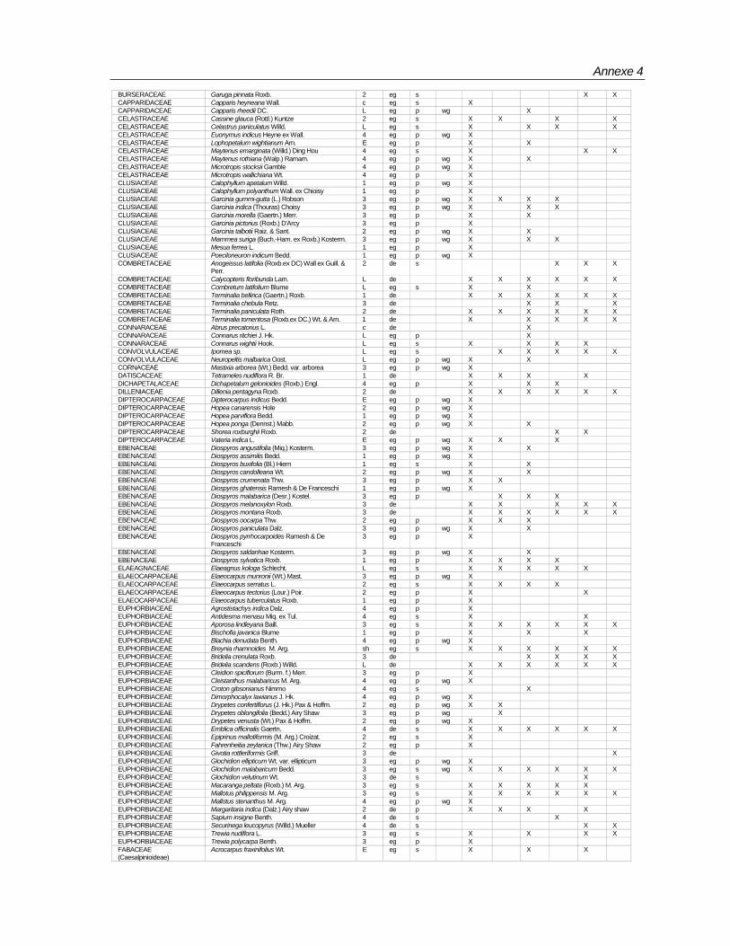
Annexe 4
BURSERACEAE Garuga pinnata Roxb. 2 eg s X X CAPPARIDACEAE Capparis heyneana Wall. c eg s X CAPPARIDACEAE Capparis rheedii DC. L eg p wg X CELASTRACEAE Cassine glauca (Rottl.) Kuntze 2 eg s X X X X CELASTRACEAE Celastrus paniculatus Willd. L eg s X X X X CELASTRACEAE Euonymus indicus Heyne ex Wall. 4 eg p wg X CELASTRACEAE Lophopetalum wightianum Arn. E eg p X X CELASTRACEAE Maytenus emarginata (Willd.) Ding Hou 4 eg s X X X CELASTRACEAE Maytenus rothiana (Walp.) Ramam. 4 eg p wg X X CELASTRACEAE Microtropis stocksii Gamble 4 eg p wg X CELASTRACEAE Microtropis wallichiana Wt. 4 eg p X CLUSIACEAE Calophyllum apetalum Willd. 1 eg p wg X CLUSIACEAE Calophyllum polyanthum Wall. ex Chioisy 1 eg p X CLUSIACEAE Garcinia gummi-gutta (L.) Robson 3 eg p wg X X X X CLUSIACEAE Garcinia indica (Thouras) Choisy 3 eg p wg X X X CLUSIACEAE Garcinia morella (Gaertn.) Merr. 3 eg p X X CLUSIACEAE Garcinia pictorius (Roxb.) D'Arcy 3 eg p X CLUSIACEAE Garcinia talbotii Raiz. & Sant. 2 eg p wg X X CLUSIACEAE Mammea suriga (Buch.-Ham. ex Roxb.) Kosterm. 3 eg p wg X X X CLUSIACEAE Mesua ferrea L. 1 eg p X CLUSIACEAE Poeciloneuron indicum Bedd. 1 eg p wg X COMBRETACEAE Anogeissus latifolia (Roxb.ex DC) Wall ex Guill. &
Perr. 2 de s X X X
COMBRETACEAE Calycopteris floribunda Lam. L de X X X X X X COMBRETACEAE Combretum latifolium Blume L eg s X X COMBRETACEAE Terminalia bellirica (Gaertn.) Roxb. 1 de X X X X X X COMBRETACEAE Terminalia chebula Retz. 3 de X X X COMBRETACEAE Terminalia paniculata Roth. 2 de X X X X X X COMBRETACEAE Terminalia tomentosa (Roxb.ex DC.) Wt. & Arn. 1 de X X X X X CONNARACEAE Abrus precatorius L. c de X CONNARACEAE Connarus ritchiei J. Hk. L eg p X CONNARACEAE Connarus wightii Hook. L eg s X X X X CONVOLVULACEAE Ipomea sp. L eg s X X X X X CONVOLVULACEAE Neuropeltis malbarica Oost. L eg p wg X X CORNACEAE Mastixia arborea (Wt.) Bedd. var. arborea 3 eg p wg X DATISCACEAE Tetrameles nudiflora R. Br. 1 de X X X X DICHAPETALACEAE Dichapetalum gelonioides (Roxb.) Engl. 4 eg p X X X DILLENIACEAE Dillenia pentagyna Roxb. 2 de X X X X X X DIPTEROCARPACEAE Dipterocarpus indicus Bedd. E eg p wg X DIPTEROCARPACEAE Hopea canarensis Hole 2 eg p wg X DIPTEROCARPACEAE Hopea parviflora Bedd. 1 eg p wg X DIPTEROCARPACEAE Hopea ponga (Dennst.) Mabb. 2 eg p wg X X DIPTEROCARPACEAE Shorea roxburghii Roxb. 2 de X X DIPTEROCARPACEAE Vateria indica L. E eg p wg X X X EBENACEAE Diospyros angustifolia (Miq.) Kosterm. 3 eg p wg X X EBENACEAE Diospyros assimilis Bedd. 1 eg p wg X EBENACEAE Diospyros buxifolia (Bl.) Hiern 1 eg s X X EBENACEAE Diospyros candolleana Wt. 2 eg p wg X X EBENACEAE Diospyros crumenata Thw. 3 eg p X X EBENACEAE Diospyros ghatensis Ramesh & De Franceschi 1 eg p wg X EBENACEAE Diospyros malabarica (Desr.) Kostel. 3 eg p X X X EBENACEAE Diospyros melanoxylon Roxb. 3 de X X X X X EBENACEAE Diospyros montana Roxb. 3 de X X X X X X EBENACEAE Diospyros oocarpa Thw. 2 eg p X X X EBENACEAE Diospyros paniculata Dalz. 3 eg p wg X X EBENACEAE Diospyros pyrrhocarpoides Ramesh & De
Franceschi 3 eg p X
EBENACEAE Diospyros saldanhae Kosterm. 3 eg p wg X X EBENACEAE Diospyros sylvatica Roxb. 1 eg p X X X X ELAEAGNACEAE Elaeagnus kologa Schlecht. L eg s X X X X X ELAEOCARPACEAE Elaeocarpus munronii (Wt.) Mast. 3 eg p wg X ELAEOCARPACEAE Elaeocarpus serratus L. 2 eg s X X X X ELAEOCARPACEAE Elaeocarpus tectorius (Lour.) Poir. 2 eg p X X ELAEOCARPACEAE Elaeocarpus tuberculatus Roxb. 1 eg p X EUPHORBIACEAE Agrostistachys indica Dalz. 4 eg p X EUPHORBIACEAE Antidesma menasu Miq. ex Tul. 4 eg s X X EUPHORBIACEAE Aporosa lindleyana Baill. 3 eg s X X X X X X EUPHORBIACEAE Bischofia javanica Blume 1 eg p X X X EUPHORBIACEAE Blachia denudata Benth. 4 eg p wg X EUPHORBIACEAE Breynia rhamnoides M. Arg. sh eg s X X X X X X EUPHORBIACEAE Bridelia crenulata Roxb. 3 de X X X X EUPHORBIACEAE Bridelia scandens (Roxb.) Willd. L de X X X X X X EUPHORBIACEAE Cleidion spiciflorum (Burm. f.) Merr. 3 eg p X EUPHORBIACEAE Cleistanthus malabaricus M. Arg. 4 eg p wg X EUPHORBIACEAE Croton gibsonianus Nimmo 4 eg s X EUPHORBIACEAE Dimorphocalyx lawianus J. Hk. 4 eg p wg X EUPHORBIACEAE Drypetes confertiflorus (J. Hk.) Pax & Hoffm. 2 eg p wg X X EUPHORBIACEAE Drypetes oblongifolia (Bedd.) Airy Shaw 3 eg p wg X EUPHORBIACEAE Drypetes venusta (Wt.) Pax & Hoffm. 2 eg p wg X EUPHORBIACEAE Emblica officinalis Gaertn. 4 de s X X X X X X EUPHORBIACEAE Epiprinus mallotiformis (M. Arg.) Croizat. 2 eg s X EUPHORBIACEAE Fahrenheitia zeylanica (Thw.) Airy Shaw 2 eg p X EUPHORBIACEAE Givotia rottleriformis Griff. 3 de X EUPHORBIACEAE Glochidion ellipticum Wt. var. ellipticum 3 eg p wg X EUPHORBIACEAE Glochidion malabaricum Bedd. 3 eg s wg X X X X X X EUPHORBIACEAE Glochidion velutinum Wt. 3 de s X EUPHORBIACEAE Macaranga peltata (Roxb.) M. Arg. 3 eg s X X X X X EUPHORBIACEAE Mallotus philippensis M. Arg. 3 eg s X X X X X X EUPHORBIACEAE Mallotus stenanthus M. Arg. 4 eg p wg X EUPHORBIACEAE Margaritaria indica (Dalz.) Airy shaw 2 de p X X X X EUPHORBIACEAE Sapium insigne Benth. 4 de s X EUPHORBIACEAE Securinega leucopyrus (Willd.) Mueller 4 de s X X EUPHORBIACEAE Trewia nudiflora L. 3 eg s X X X X EUPHORBIACEAE Trewia polycarpa Benth. 3 eg p X FABACEAE (Caesalpinioideae)
Acrocarpus fraxinifolius Wt. E eg s X X X
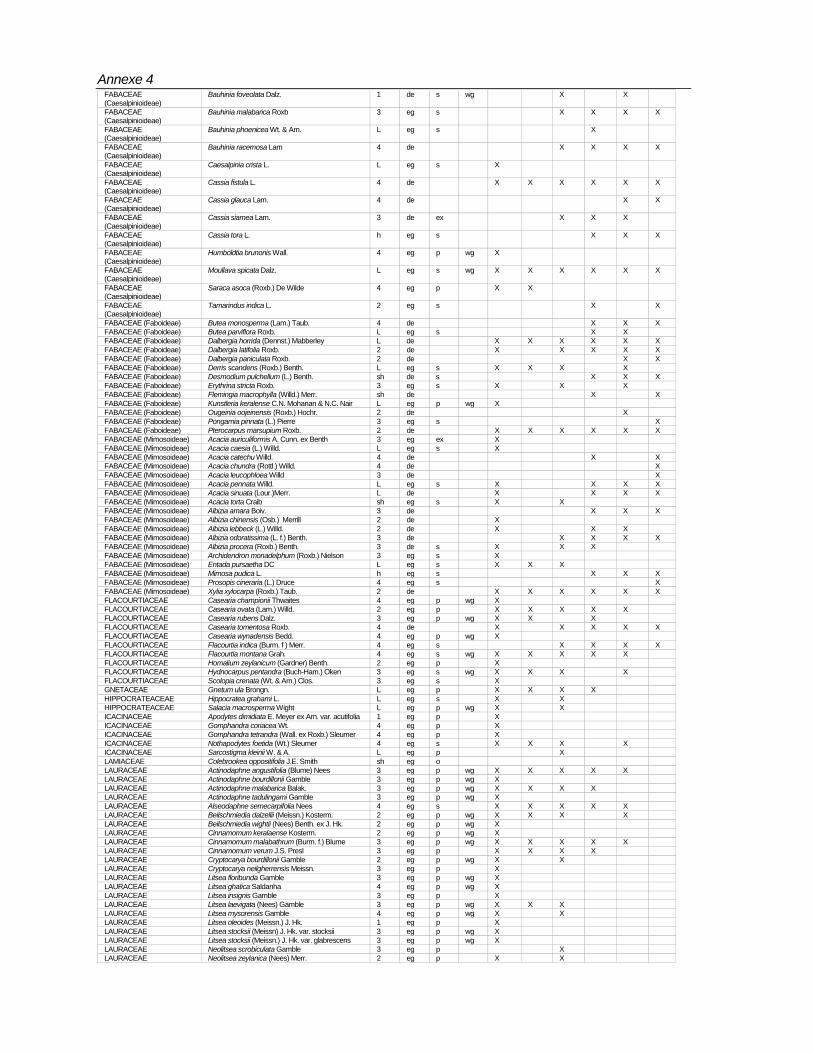
Annexe 4
FABACEAE (Caesalpinioideae)
Bauhinia foveolata Dalz. 1 de s wg X X
FABACEAE (Caesalpinioideae)
Bauhinia malabarica Roxb 3 eg s X X X X
FABACEAE (Caesalpinioideae)
Bauhinia phoenicea Wt. & Arn. L eg s X
FABACEAE (Caesalpinioideae)
Bauhinia racemosa Lam 4 de X X X X
FABACEAE (Caesalpinioideae)
Caesalpinia crista L. L eg s X
FABACEAE (Caesalpinioideae)
Cassia fistula L. 4 de X X X X X X
FABACEAE (Caesalpinioideae)
Cassia glauca Lam. 4 de X X
FABACEAE (Caesalpinioideae)
Cassia siamea Lam. 3 de ex X X X
FABACEAE (Caesalpinioideae)
Cassia tora L. h eg s X X X
FABACEAE (Caesalpinioideae)
Humboldtia brunonis Wall. 4 eg p wg X
FABACEAE (Caesalpinioideae)
Moullava spicata Dalz. L eg s wg X X X X X X
FABACEAE (Caesalpinioideae)
Saraca asoca (Roxb.) De Wilde 4 eg p X X
FABACEAE (Caesalpinioideae)
Tamarindus indica L. 2 eg s X X
FABACEAE (Faboideae) Butea monosperma (Lam.) Taub. 4 de X X X FABACEAE (Faboideae) Butea parviflora Roxb. L eg s X X FABACEAE (Faboideae) Dalbergia horrida (Dennst.) Mabberley L de X X X X X X FABACEAE (Faboideae) Dalbergia latifolia Roxb. 2 de X X X X X FABACEAE (Faboideae) Dalbergia paniculata Roxb. 2 de X X FABACEAE (Faboideae) Derris scandens (Roxb.) Benth. L eg s X X X X FABACEAE (Faboideae) Desmodium pulchellum (L.) Benth. sh de s X X X FABACEAE (Faboideae) Erythrina stricta Roxb. 3 eg s X X X FABACEAE (Faboideae) Flemingia macrophylla (Willd.) Merr. sh de X X FABACEAE (Faboideae) Kunstleria keralense C.N. Mohanan & N.C. Nair L eg p wg X FABACEAE (Faboideae) Ougeinia oojeinensis (Roxb.) Hochr. 2 de X FABACEAE (Faboideae) Pongamia pinnata (L.) Pierre 3 eg s X FABACEAE (Faboideae) Pterocarpus marsupium Roxb. 2 de X X X X X X FABACEAE (Mimosoideae) Acacia auriculiformis A. Cunn. ex Benth 3 eg ex X FABACEAE (Mimosoideae) Acacia caesia (L.) Willd. L eg s X FABACEAE (Mimosoideae) Acacia catechu Willd. 4 de X X FABACEAE (Mimosoideae) Acacia chundra (Rottl.) Willd. 4 de X FABACEAE (Mimosoideae) Acacia leucophloea Willd 3 de X FABACEAE (Mimosoideae) Acacia pennata Willd. L eg s X X X X FABACEAE (Mimosoideae) Acacia sinuata (Lour.)Merr. L de X X X X FABACEAE (Mimosoideae) Acacia torta Craib sh eg s X X FABACEAE (Mimosoideae) Albizia amara Boiv. 3 de X X X FABACEAE (Mimosoideae) Albizia chinensis (Osb.) Merrill 2 de X FABACEAE (Mimosoideae) Albizia lebbeck (L.) Willd. 2 de X X X FABACEAE (Mimosoideae) Albizia odoratissima (L. f.) Benth. 3 de X X X X FABACEAE (Mimosoideae) Albizia procera (Roxb.) Benth. 3 de s X X X FABACEAE (Mimosoideae) Archidendron monadelphum (Roxb.) Nielson 3 eg s X FABACEAE (Mimosoideae) Entada pursaetha DC L eg s X X X FABACEAE (Mimosoideae) Mimosa pudica L. h eg s X X X FABACEAE (Mimosoideae) Prosopis cineraria (L.) Druce 4 eg s X FABACEAE (Mimosoideae) Xylia xylocarpa (Roxb.) Taub. 2 de X X X X X X FLACOURTIACEAE Casearia championii Thwaites 4 eg p wg X FLACOURTIACEAE Casearia ovata (Lam.) Willd. 2 eg p X X X X X FLACOURTIACEAE Casearia rubens Dalz. 3 eg p wg X X X FLACOURTIACEAE Casearia tomentosa Roxb. 4 de X X X X X FLACOURTIACEAE Casearia wynadensis Bedd. 4 eg p wg X FLACOURTIACEAE Flacourtia indica (Burm. f ) Merr. 4 eg s X X X X FLACOURTIACEAE Flacourtia montana Grah. 4 eg s wg X X X X X FLACOURTIACEAE Homalium zeylanicum (Gardner) Benth. 2 eg p X FLACOURTIACEAE Hydnocarpus pentandra (Buch-Ham.) Oken 3 eg s wg X X X X FLACOURTIACEAE Scolopia crenata (Wt. & Arn.) Clos. 3 eg s X GNETACEAE Gnetum ula Brongn. L eg p X X X X HIPPOCRATEACEAE Hippocratea grahami L. L eg s X X HIPPOCRATEACEAE Salacia macrosperma Wight L eg p wg X X ICACINACEAE Apodytes dimidiata E. Meyer ex Arn. var. acutifolia 1 eg p X ICACINACEAE Gomphandra coriacea Wt. 4 eg p X ICACINACEAE Gomphandra tetrandra (Wall. ex Roxb.) Sleumer 4 eg p X ICACINACEAE Nothapodytes foetida (Wt.) Sleumer 4 eg s X X X X ICACINACEAE Sarcostigma kleinii W. & A. L eg p X LAMIACEAE Colebrookea oppositifolia J.E. Smith sh eg o LAURACEAE Actinodaphne angustifolia (Blume) Nees 3 eg p wg X X X X X LAURACEAE Actinodaphne bourdillonii Gamble 3 eg p wg X LAURACEAE Actinodaphne malabarica Balak. 3 eg p wg X X X X LAURACEAE Actinodaphne tadulingami Gamble 3 eg p wg X LAURACEAE Alseodaphne semecarpifolia Nees 4 eg s X X X X X LAURACEAE Beilschmiedia dalzellii (Meissn.) Kosterm. 2 eg p wg X X X X LAURACEAE Beilschmiedia wightii (Nees) Benth. ex J. Hk. 2 eg p wg X LAURACEAE Cinnamomum keralaense Kosterm. 2 eg p wg X LAURACEAE Cinnamomum malabathrum (Burm. f.) Blume 3 eg p wg X X X X X LAURACEAE Cinnamomum verum J.S. Presl 3 eg p X X X X LAURACEAE Cryptocarya bourdillonii Gamble 2 eg p wg X X LAURACEAE Cryptocarya neilgherrensis Meissn. 3 eg p X LAURACEAE Litsea floribunda Gamble 3 eg p wg X LAURACEAE Litsea ghatica Saldanha 4 eg p wg X LAURACEAE Litsea insignis Gamble 3 eg p X LAURACEAE Litsea laevigata (Nees) Gamble 3 eg p wg X X X LAURACEAE Litsea mysorensis Gamble 4 eg p wg X X LAURACEAE Litsea oleoides (Meissn.) J. Hk. 1 eg p X LAURACEAE Litsea stocksii (Meissn) J. Hk. var. stocksii 3 eg p wg X LAURACEAE Litsea stocksii (Meissn.) J. Hk. var. glabrescens 3 eg p wg X LAURACEAE Neolitsea scrobiculata Gamble 3 eg p X LAURACEAE Neolitsea zeylanica (Nees) Merr. 2 eg p X X
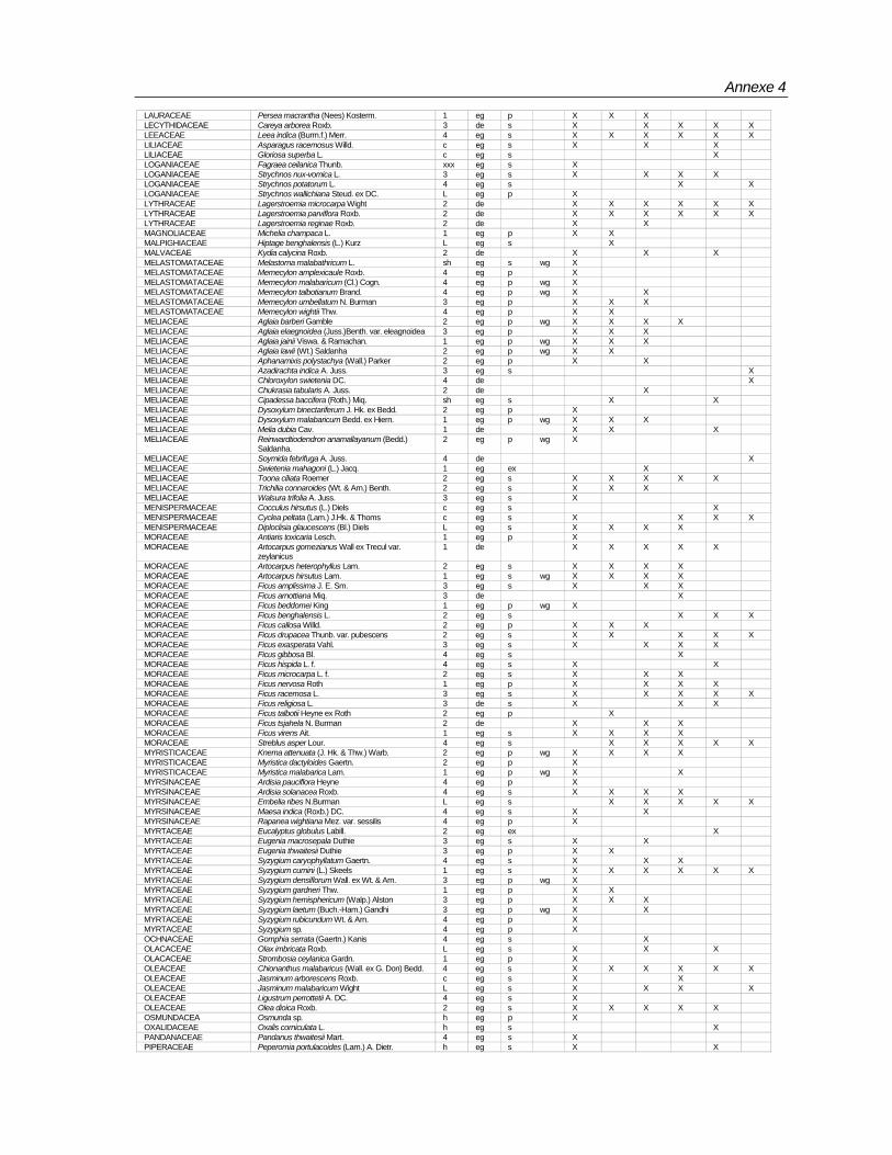
Annexe 4
LAURACEAE Persea macrantha (Nees) Kosterm. 1 eg p X X X LECYTHIDACEAE Careya arborea Roxb. 3 de s X X X X X LEEACEAE Leea indica (Burm.f.) Merr. 4 eg s X X X X X X LILIACEAE Asparagus racemosus Willd. c eg s X X X LILIACEAE Gloriosa superba L. c eg s X LOGANIACEAE Fagraea ceilanica Thunb. xxx eg s X LOGANIACEAE Strychnos nux-vomica L. 3 eg s X X X X LOGANIACEAE Strychnos potatorum L. 4 eg s X X LOGANIACEAE Strychnos wallichiana Steud. ex DC. L eg p X LYTHRACEAE Lagerstroemia microcarpa Wight 2 de X X X X X X LYTHRACEAE Lagerstroemia parviflora Roxb. 2 de X X X X X X LYTHRACEAE Lagerstroemia reginae Roxb. 2 de X X MAGNOLIACEAE Michelia champaca L. 1 eg p X X MALPIGHIACEAE Hiptage benghalensis (L.) Kurz L eg s X MALVACEAE Kydia calycina Roxb. 2 de X X X MELASTOMATACEAE Melastoma malabathricum L. sh eg s wg X MELASTOMATACEAE Memecylon amplexicaule Roxb. 4 eg p X MELASTOMATACEAE Memecylon malabaricum (Cl.) Cogn. 4 eg p wg X MELASTOMATACEAE Memecylon talbotianum Brand. 4 eg p wg X X MELASTOMATACEAE Memecylon umbellatum N. Burman 3 eg p X X X MELASTOMATACEAE Memecylon wightii Thw. 4 eg p X X MELIACEAE Aglaia barberi Gamble 2 eg p wg X X X X MELIACEAE Aglaia elaegnoidea (Juss.)Benth. var. eleagnoidea 3 eg p X X X MELIACEAE Aglaia jainii Viswa. & Ramachan. 1 eg p wg X X X MELIACEAE Aglaia lawii (Wt.) Saldanha 2 eg p wg X X MELIACEAE Aphanamixis polystachya (Wall.) Parker 2 eg p X X MELIACEAE Azadirachta indica A. Juss. 3 eg s X MELIACEAE Chloroxylon swietenia DC. 4 de X MELIACEAE Chukrasia tabularis A. Juss. 2 de X MELIACEAE Cipadessa baccifera (Roth.) Miq. sh eg s X X MELIACEAE Dysoxylum binectariferum J. Hk. ex Bedd. 2 eg p X MELIACEAE Dysoxylum malabaricum Bedd. ex Hiern. 1 eg p wg X X X MELIACEAE Melia dubia Cav. 1 de X X X MELIACEAE Reinwardtiodendron anamallayanum (Bedd.)
Saldanha. 2 eg p wg X
MELIACEAE Soymida febrifuga A. Juss. 4 de X MELIACEAE Swietenia mahagoni (L.) Jacq. 1 eg ex X MELIACEAE Toona ciliata Roemer 2 eg s X X X X X MELIACEAE Trichilia connaroides (Wt. & Arn.) Benth. 2 eg s X X X MELIACEAE Walsura trifolia A. Juss. 3 eg s X MENISPERMACEAE Cocculus hirsutus (L.) Diels c eg s X MENISPERMACEAE Cyclea peltata (Lam.) J.Hk. & Thoms c eg s X X X X MENISPERMACEAE Diploclisia glaucescens (Bl.) Diels L eg s X X X X MORACEAE Antiaris toxicaria Lesch. 1 eg p X MORACEAE Artocarpus gomezianus Wall ex Trecul var.
zeylanicus 1 de X X X X X
MORACEAE Artocarpus heterophyllus Lam. 2 eg s X X X X MORACEAE Artocarpus hirsutus Lam. 1 eg s wg X X X X MORACEAE Ficus amplissima J. E. Sm. 3 eg s X X X MORACEAE Ficus arnottiana Miq. 3 de X MORACEAE Ficus beddomei King 1 eg p wg X MORACEAE Ficus benghalensis L. 2 eg s X X X MORACEAE Ficus callosa Willd. 2 eg p X X X MORACEAE Ficus drupacea Thunb. var. pubescens 2 eg s X X X X X MORACEAE Ficus exasperata Vahl. 3 eg s X X X X MORACEAE Ficus gibbosa Bl. 4 eg s X MORACEAE Ficus hispida L. f. 4 eg s X X MORACEAE Ficus microcarpa L. f. 2 eg s X X X MORACEAE Ficus nervosa Roth 1 eg p X X X X MORACEAE Ficus racemosa L. 3 eg s X X X X X MORACEAE Ficus religiosa L. 3 de s X X X MORACEAE Ficus talbotii Heyne ex Roth 2 eg p X MORACEAE Ficus tsjahela N. Burman 2 de X X X MORACEAE Ficus virens Ait. 1 eg s X X X X MORACEAE Streblus asper Lour. 4 eg s X X X X X MYRISTICACEAE Knema attenuata (J. Hk. & Thw.) Warb. 2 eg p wg X X X X MYRISTICACEAE Myristica dactyloides Gaertn. 2 eg p X MYRISTICACEAE Myristica malabarica Lam. 1 eg p wg X X MYRSINACEAE Ardisia pauciflora Heyne 4 eg p X MYRSINACEAE Ardisia solanacea Roxb. 4 eg s X X X X MYRSINACEAE Embelia ribes N.Burman L eg s X X X X X MYRSINACEAE Maesa indica (Roxb.) DC. 4 eg s X X MYRSINACEAE Rapanea wightiana Mez. var. sessilis 4 eg p X MYRTACEAE Eucalyptus globulus Labill. 2 eg ex X MYRTACEAE Eugenia macrosepala Duthie 3 eg s X X MYRTACEAE Eugenia thwaitesii Duthie 3 eg p X X MYRTACEAE Syzygium caryophyllatum Gaertn. 4 eg s X X X MYRTACEAE Syzygium cumini (L.) Skeels 1 eg s X X X X X X MYRTACEAE Syzygium densiflorum Wall. ex Wt. & Arn. 3 eg p wg X MYRTACEAE Syzygium gardneri Thw. 1 eg p X X MYRTACEAE Syzygium hemisphericum (Walp.) Alston 3 eg p X X X MYRTACEAE Syzygium laetum (Buch.-Ham.) Gandhi 3 eg p wg X X MYRTACEAE Syzygium rubicundum Wt. & Arn. 4 eg p X MYRTACEAE Syzygium sp. 4 eg p X OCHNACEAE Gomphia serrata (Gaertn.) Kanis 4 eg s X OLACACEAE Olax imbricata Roxb. L eg s X X X OLACACEAE Strombosia ceylanica Gardn. 1 eg p X OLEACEAE Chionanthus malabaricus (Wall. ex G. Don) Bedd. 4 eg s X X X X X X OLEACEAE Jasminum arborescens Roxb. c eg s X X OLEACEAE Jasminum malabaricum Wight L eg s X X X X OLEACEAE Ligustrum perrottetii A. DC. 4 eg s X OLEACEAE Olea dioica Roxb. 2 eg s X X X X X OSMUNDACEA Osmunda sp. h eg p X OXALIDACEAE Oxalis corniculata L. h eg s X PANDANACEAE Pandanus thwaitesii Mart. 4 eg s X PIPERACEAE Peperomia portulacoides (Lam.) A. Dietr. h eg s X X

Annexe 4
PIPERACEAE Piper hymenophyllum Miq. c eg p wg X X X X PIPERACEAE Piper sp. c eg p X X PITTOSPORACEAE Pittosporum dasycaulon Miq. 3 eg p wg POACEAE Bambusa arundinacea (Retz.) Willd. 4 de s X X X POLGONACEAE Polygonum chinense L. h eg s X PROTEACEAE Grevillea robusta R. Br. 2 eg ex X PTERIDACEAE Pteris quadriaurita Retz. h eg o X RANUNCULACEAE Clematis gouriana Roxb. c de o X X RHAMNACEAE Scutia myrtina Kurz. L eg s X RHAMNACEAE Ventilago maderaspatana Gaertn. L eg s X X X X X X RHAMNACEAE Ziziphus glaberrima Sant. L eg s X X X X RHAMNACEAE Ziziphus nummularia Wt. sh eg s X RHAMNACEAE Ziziphus oenoplia (L.) Mill. L eg s X X X X X X RHAMNACEAE Ziziphus rugosa Lam. 4 eg s X X X X X X RHAMNACEAE Ziziphus xylopyrus (Retz.) Willd. 4 eg s X X RHIZOPHORACEAE Carallia brachiata (Lour.) Merr. 2 eg p X X X X ROSACEAE Prunus ceylanica (Wt.) Miq. 2 eg p X RUBIACEAE Canthium angustifolium Roxb. L eg p X X X X X RUBIACEAE Canthium dicoccum (Gaertn.) Teissm. var.
dicoccum 3 eg s X X X X X
RUBIACEAE Canthium parviflorum Lamk. 4 eg s X X RUBIACEAE Catunaregam dumetorum (Retz.)Tirven. 4 de X X X X X X RUBIACEAE Chasalia ophioxyloides (Wall.) Craib h eg p X RUBIACEAE Gardenia gummifera L.f. 4 eg s X RUBIACEAE Gardenia latifolia Aiton 4 eg s X X RUBIACEAE Gardenia resinifera Roth. 4 eg s X RUBIACEAE Haldina cordifolia (Roxb.) Ridsdale 1 de X X X X X RUBIACEAE Hymenodictyon orixense (Roxb.) Mabberly 2 de s X X RUBIACEAE Ixora arborea Roxb. ex Smith 4 eg s X X RUBIACEAE Ixora brachiata Roxb. ex DC. 3 eg s wg X X X X X X RUBIACEAE Ixora coccinia L. sh eg s X X X RUBIACEAE Ixora nigricans Br. ex Wt. & Arn. 4 eg p X X X RUBIACEAE Ixora polyantha Wt. sh eg p wg X X RUBIACEAE Lasianthus acuminatus Wt. sh eg p wg X RUBIACEAE Meyna laxiflora Robyns 4 eg s X X X X X X RUBIACEAE Mitragyna parvifolia (Roxb.) Korth. 2 de s X X X X X RUBIACEAE Mussaenda frondosa Linn. L eg s X X X X RUBIACEAE Neolamarkia cadamba (Roxb.) Bosser 1 eg p X RUBIACEAE Pavetta indica L. 4 eg s X RUBIACEAE Pavetta tomentosa Roxb. ex J.E. Smith 4 de X X X RUBIACEAE Psychotria dalzellii J. Hk. 4 eg p wg X X X RUBIACEAE Psychotria flavida Talbot 4 eg p X X RUBIACEAE Psychotria nigra (Gaertn.) Alston 4 eg p wg X X RUBIACEAE Psychotria octosulcata Talbot sh eg p wg X RUBIACEAE Psychotria truncata Wall. 4 eg p wg X RUBIACEAE Randia rugulosa (Thw.)J.Hk. L eg p X X RUBIACEAE Tamilnadia uliginosa (Retz.) Tirven. 4 eg s X RUBIACEAE Tarenna asiatica (L.) Kuntze ex K. Schum. var.
rigida sh eg s X
RUBIACEAE Tricalysia apiocarpa (Dalz.) Gamble 3 eg p wg X RUBIACEAE Wendlandia thyrsoidea (Schultes) Steud. 4 eg s X X RUTACEAE Aegle marmelos L. 3 de X RUTACEAE Atalantia wightii Tanaka 4 eg p wg X X X X RUTACEAE Clausena dentata (Willd.) R. & S. 4 eg s X X X RUTACEAE Clausena indica Oliver 4 eg s X X X X RUTACEAE Euodia lunu-ankenda (Gaertn.) Merr. 3 eg s X X X X X RUTACEAE Glycosmis macrocarpa Wt. 3 eg p wg X X RUTACEAE Glycosmis pentaphylla Corr. 4 eg s X X X X RUTACEAE Luvunga sarmentosa (Blume) Kurz L eg p X RUTACEAE Murraya koenigii (L.) Spreng. 4 eg s X X X X RUTACEAE Naringi crenulata (Roxb.) Nicolson 4 eg s X X RUTACEAE Paramignya monophylla Wight L eg p X X X X X RUTACEAE Toddalia asiatica (L.) Lam. L eg s X X X X X RUTACEAE Vepris bilocularis (Wt. & Arn.) Engl. 3 eg p wg X X RUTACEAE Zanthoxylum ovalifolium Wt. L eg s X X RUTACEAE Zanthoxylum rhetsa (Roxb.) DC. 3 de X X X X SANTALACEAE Osyris quadripartita Salz. ex Decne. 4 eg s X SANTALACEAE Santalum album L. 4 eg s X X X SANTALACEAE Scleropyrum pentandrum (Denn.) Mabb. 4 eg s X SAPINDACEAE Allophylus cobbe (L.) Raeusch 4 eg s X X X X SAPINDACEAE Dimocarpus longan Lour. 1 eg s X X X X SAPINDACEAE Dodonaea viscosa (L.)Jacq sh eg s X SAPINDACEAE Harpullia arborea (Blanco) Radlk. 3 eg p X X X X SAPINDACEAE Lepisanthes decipiens Radlk. 4 eg p X X X SAPINDACEAE Sapindus laurifolia Vahl 3 de X X X X SAPINDACEAE Schleichera oleosa (Lour.) Oken 2 de X X X X X X SAPOTACEAE Chrysophyllum lanceolatum (Blume) DC. 1 eg p X X SAPOTACEAE Isonandra lanceolata Wt. 4 eg p X SAPOTACEAE Madhuca longifolia (Koen.) Macbride var. latifolia 2 de X X X X X SAPOTACEAE Madhuca neriifolia (Moon.) Lam. 3 eg p X SAPOTACEAE Mimusops elengi L. 1 eg p X X X X X SAPOTACEAE Palaquium ellipticum (Dalz.) Baillon 1 eg p wg X SAPOTACEAE Xantolis tomentosa (Roxb.) Raf. 2 eg p X X X X X X SELAGINELACEAE Selaginela sp. h eg p X SIMARUBACEAE Ailanthus excelsa Roxb. 3 de ex X X SIMARUBACEAE Ailanthus triphysa (Dennst.) Alston 1 de X X X X SMILACACEAE Smilax zeylancia L. c eg s X X X X X X SOLANACEAE Solanum torvum Sw. sh eg s X STAPHYLACEAE Turpinia malabarica Gamble 3 eg p wg X STERCULIACEAE Helicteres isora L. 4 de X STERCULIACEAE Pterospermum diversifolium Blume 2 eg s X X STERCULIACEAE Pterospermum reticulatum Wt. & Arn. 2 eg s wg X X X X STERCULIACEAE Sterculia colorata R. Br. 3 de X STERCULIACEAE Sterculia guttata Roxb. 2 de X X X X X STERCULIACEAE Sterculia urens Roxb. 3 de X X SYMPLOCACEAE Symplocos cochinchinensis (Lour.) Moore var.
laurina 4 eg s X X
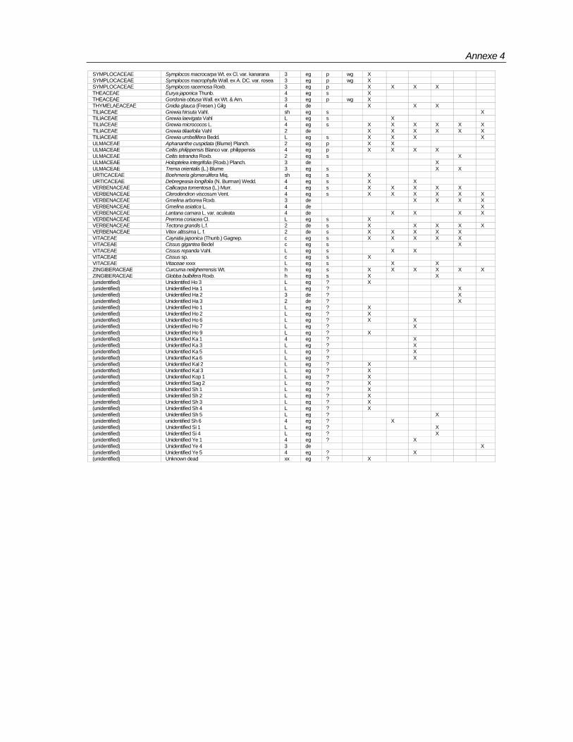
Annexe 4
SYMPLOCACEAE Symplocos macrocarpa Wt. ex Cl. var. kanarana 3 eg p wg X SYMPLOCACEAE Symplocos macrophylla Wall. ex A. DC. var. rosea 3 eg p wg X SYMPLOCACEAE Symplocos racemosa Roxb. 3 eg p X X X X THEACEAE Eurya japonica Thunb. 4 eg s X THEACEAE Gordonia obtusa Wall. ex Wt. & Arn. 3 eg p wg X THYMELAEACEAE Gnidia glauca (Fresen.) Gilg 4 de X X X TILIACEAE Grewia hirsuta Vahl. sh eg s X TILIACEAE Grewia laevigata Vahl L eg s X TILIACEAE Grewia micrococos L. 4 eg s X X X X X X TILIACEAE Grewia tiliaefolia Vahl 2 de X X X X X X TILIACEAE Grewia umbellifera Bedd. L eg s X X X X ULMACEAE Aphananthe cuspidata (Blume) Planch. 2 eg p X X ULMACEAE Celtis philippensis Blanco var. philippensis 4 eg p X X X X ULMACEAE Celtis tetrandra Roxb. 2 eg s X ULMACEAE Holoptelea integrifolia (Roxb.) Planch. 3 de X ULMACEAE Trema orientalis (L.) Blume 3 eg s X X URTICACEAE Boehmeria glomerulifera Miq. sh eg s X URTICACEAE Debregeasia longifolia (N. Burman) Wedd. 4 eg s X X VERBENACEAE Callicarpa tomentosa (L.) Murr. 4 eg s X X X X X VERBENACEAE Clerodendron viscosum Vent. 4 eg s X X X X X X VERBENACEAE Gmelina arborea Roxb. 3 de X X X X VERBENACEAE Gmelina asiatica L. 4 de X VERBENACEAE Lantana camara L. var. aculeata 4 de X X X X VERBENACEAE Premna coriacea Cl. L eg s X VERBENACEAE Tectona grandis L.f. 2 de s X X X X X VERBENACEAE Vitex altissima L. f. 2 de s X X X X X VITACEAE Cayratia japonica (Thunb.) Gagnep. c eg s X X X X X VITACEAE Cissus gigantea Bedel c eg s X VITACEAE Cissus repanda Vahl. L eg s X X VITACEAE Cissus sp. c eg s X VITACEAE Vitaceae xxxx L eg s X X ZINGIBERACEAE Curcuma neilgherrensis Wt. h eg s X X X X X X ZINGIBERACEAE Globba bulbifera Roxb. h eg s X X (unidentified) Unidentifed Ho 3 L eg ? X (unidentified) Unidentified Ha 1 L eg ? X (unidentified) Unidentified Ha 2 3 de ? X (unidentified) Unidentified Ha 3 2 de ? X (unidentified) Unidentified Ho 1 L eg ? X (unidentified) Unidentified Ho 2 L eg ? X (unidentified) Unidentified Ho 6 L eg ? X X (unidentified) Unidentified Ho 7 L eg ? X (unidentified) Unidentified Ho 9 L eg ? X (unidentified) Unidentified Ka 1 4 eg ? X (unidentified) Unidentified Ka 3 L eg ? X (unidentified) Unidentified Ka 5 L eg ? X (unidentified) Unidentified Ka 6 L eg ? X (unidentified) Unidentified Kal 2 L eg ? X (unidentified) Unidentified Kal 3 L eg ? X (unidentified) Unidentified Kop 1 L eg ? X (unidentified) Unidentified Sag 2 L eg ? X (unidentified) Unidentified Sh 1 L eg ? X (unidentified) Unidentified Sh 2 L eg ? X (unidentified) Unidentified Sh 3 L eg ? X (unidentified) Unidentified Sh 4 L eg ? X (unidentified) Unidentified Sh 5 L eg ? X (unidentified) unidentified Sh 6 4 eg ? X (unidentified) Unidentified Si 1 L eg ? X (unidentified) Unidentified Si 4 L eg ? X (unidentified) Unidentified Ye 1 4 eg ? X (unidentified) Unidentified Ye 4 3 de X (unidentified) Unidentified Ye 5 4 eg ? X (unidentified) Unknown dead xx eg ? X

Pondy Papers in Ecology
1. CLAIRE ELOUARD, FRANÇOIS HOULLIER, JEAN-PIERRE PASCAL, RAPHAEL PÉLISSIER, B.R. RAMESH. Dynamics of the dense moist evergreen forests. Long Term Monitoring of an Experimental Station in Kodagu District (Karnataka, India), 1997, n ° l , 23 p. http://hal.archives-ouvertes.fr/hal-00373536/fr/
2. FRANÇOIS HOULLIER, YVES CARAGLIO, MURIEL DURAND. Modelling Tree Architecture and Forest Dynamics. A Research Project in the dense moist evergreen forests of the Western Ghats (South India), 1997, n°2, 37 p. http://hal.archives-ouvertes.fr/hal-00373538/fr/
3. MURIEL DURAND. Architecture and growth strategy of two evergreen species of the Western Ghats (South India), Knema attenuata (J. Hk. & Thw.) Warb. (Myristicacece) and Vateria indica L. (Dipterocarpacece) 1997, n° 3, 39 p. http://hal.archives-ouvertes.fr/hal-00373540/fr/
4. FRANÇOIS HOULLIER, RANI M. KRISHNAN, CLAIRE ELOUARD. Assessment of Forest Biological Diversity. A FAO training course. 1. Lecture Notes 1998, n° 4, 102 p. http://hal.archives-ouvertes.fr/hal-00373545/fr/
5. CLAIRE ELOUARD, RANI M. KRISHNAN. Assessment of Forest Biological Diversity. A FAO training course. 2. Case study in India, 1999, n° 5, 75 p. http://hal.archives-ouvertes.fr/hal-00373548/fr/
6. B. R. RAMESH, MOHAN SEETHARAM, M. C. GUERO, R. MICHON. Assessment and Conservation of Forest Biodiversity in the Western Ghats of Karnataka, India. 1. General Introduction and Forest Land Cover and Land Use Changes (1977-1997), 2009, n° 6, pp. 1-64 p.
7. B. R. RAMESH, M. H. SWAMINATH, SANTHOSHAGOUDA PATIL, S. ARAVAJY, CLAIRE ELOUARD. Assessment and Conservation of Forest Biodiversity in the Western Ghats of Karnataka, India. 2. Assessment of Tree Biodiversity, Logging Impact and General Discussion. 2009, n° 7, pp. 65-121.