copyright © 2004-2018 by geoslope international,...

2

Copyright © 2004-2018 by GEOSLOPE International, Ltd.

All rights reserved. No part of this work may be reproduced or transmitted in any form or by any means,

electronic or mechanical, including photocopying, recording, or by any information storage or retrieval

system, without the prior written permission of GEOSLOPE International, Ltd.

Trademarks:

GEOSLOPE, GeoStudio, SLOPE/W, SEEP/W, SIGMA/W, QUAKE/W, CTRAN/W, TEMP/W, AIR/W and

VADOSE/W are trademarks or registered trademarks of GEOSLOPE International Ltd. in Canada and

other countries. Other trademarks are the property of their respective owners.

Recommended citation:

GEOSLOPE International Ltd. 2017. Heat and mass transfer modeling with GeoStudio 2018 (Second

Edition). Calgary, Alberta, Canada.

Updated January 2018; First Published August 2017

GEOSLOPE International Ltd. | www.geoslope.com

1200, 700 - 6th Ave SW, Calgary, AB, Canada T2P 0T8

Main: +1 403 269 2002 | Fax: +1 888 436 2239

http://www.geoslope.com/

3

Contents Symbols ......................................................................................................................................................... 6

Preface ........................................................................................................................................................ 10

1 GeoStudio Overview ........................................................................................................................... 11

2 Finite Element Approach for Field Problems ...................................................................................... 13

3 Water Transfer with SEEP/W .............................................................................................................. 14

3.1 Theory ......................................................................................................................................... 14

3.2 Material Models .......................................................................................................................... 18

3.2.1 Saturated-Only .................................................................................................................... 18

3.2.2 Saturated-Unsaturated ....................................................................................................... 18

3.2.3 Estimation Techniques ........................................................................................................ 20

3.3 Boundary Conditions ................................................................................................................... 21

3.3.1 Potential Seepage Face Review .......................................................................................... 21

3.3.2 Total Head versus Volume .................................................................................................. 21

3.3.3 Unit Gradient ...................................................................................................................... 22

3.3.4 Land-Climate Interaction .................................................................................................... 22

3.3.5 Diurnal Distributions ........................................................................................................... 28


3.4 Convergence ............................................................................................................................... 30

3.4.1 Water Balance Error ............................................................................................................ 30

3.4.2 Conductivity Comparison .................................................................................................... 30

4 Heat Transfer with TEMP/W ............................................................................................................... 31

4.1 Theory ......................................................................................................................................... 31

4.2 Material Models .......................................................................................................................... 34

4.2.1 Full Thermal ........................................................................................................................ 34

4.2.2 Simplified Thermal .............................................................................................................. 35

4.2.3 Coupled Convective ............................................................................................................ 35



4.3.1 Surface Energy Balance ....................................................................................................... 38

4.3.2 n-Factor ............................................................................................................................... 46

4.3.3 Convective Surface and Thermosyphon ............................................................................. 47


4

5 Air Transfer with AIR/W ...................................................................................................................... 50

5.1 Theory ......................................................................................................................................... 50

5.2 Material Models .......................................................................................................................... 52

5.2.1 Single Phase ........................................................................................................................ 52

5.2.2 Dual Phase ........................................................................................................................... 53



5.3.1 Barometric Air Pressure ...................................................................................................... 53

6 Solute and Gas Transfer with CTRAN/W ............................................................................................. 55

6.1 Theory ......................................................................................................................................... 55

6.1.1 Solute Transfer .................................................................................................................... 55

6.1.2 Gas Transfer ........................................................................................................................ 57

6.2 Material Models .......................................................................................................................... 58

6.2.1 Solute Transfer .................................................................................................................... 58

6.2.2 Gas Transfer ........................................................................................................................ 59


6.3.1 Source Concentration ......................................................................................................... 60

6.3.2 Free Exit Mass Flux .............................................................................................................. 60

6.4 Convergence ............................................................................................................................... 60

6.4.1 Dimensionless Numbers ..................................................................................................... 60

7 References .......................................................................................................................................... 62

Appendix I Formulation Fundamentals ................................................................................................. 67

I.1 Governing Equation .................................................................................................................... 68

I.1.1 Conservation of Mass Requirement ....................................................................................... 68

I.1.2 Conservation of Energy Requirement ..................................................................................... 69

I.2 Domain Discretization ................................................................................................................. 70

I.3 Primary Variable Approximation ................................................................................................ 71

I.4 Element Equations ...................................................................................................................... 71

I.5 Global Equations ......................................................................................................................... 72

I.6 Constitutive Behaviour................................................................................................................ 73

I.6.1 Functional Relationships ......................................................................................................... 74

I.6.2 Add-ins .................................................................................................................................... 74

I.7 Boundary Conditions ................................................................................................................... 74

5

I.7.1 Types ....................................................................................................................................... 75

I.7.2 Add-ins .................................................................................................................................... 75

I.8 Convergence ............................................................................................................................... 76

I.8.1 Significant Figures ................................................................................................................... 76

I.8.2 Maximum Difference .............................................................................................................. 76

I.8.3 Under-Relaxation .................................................................................................................... 76

I.8.4 Verifying Convergence ............................................................................................................ 77

Appendix II Numerical Modelling Best Practice ..................................................................................... 78

6

Symbols 𝜶 Albedo 𝜶 Dispersivity of soil/medium, m

in longitudinal direction, 𝛼𝐿 in air phase, 𝛼𝐿𝑎 in water phase, 𝛼𝐿𝑤 in transverse direction, 𝛼𝑇 in air phase, 𝛼𝑇𝑎 in water phase, 𝛼𝑇𝑤

𝜶 Rotation angle of x-y plane, degrees 𝜶 Slope angle for surface mass balance

𝜶𝒓𝒘 Root water extraction reduction factor 𝜶𝒘 Volumetric coefficient of thermal

expansion at constant pressure, /K 𝜷 Soil structure compressibility, /kPa

𝜷𝒘 Isothermal compressibility of water, 4.8x10-10 /kPa at 10 ⁰C

𝜸 Psychrometric constant, 0.0665 kPa/C 𝚪 Slope of the saturation vapor pressure

vs. temperature curve, kPa/C 𝜹 Solar declination, radians

𝚫𝒕 Time increment 𝚫𝒙 Nodal spacing 𝜺

Emissivity air emissivity, 휀𝑎

𝜼 Dynamic viscosity, kg/s/m 𝜽 Normalized time for sinusoidal radiation

distribution, radians 𝜽 Volumetric content, m3/m3

water content, 𝜃𝑤 unfrozen water content, 𝜃𝑢𝑤𝑐 at a given temperature, 𝜃𝑢𝑤𝑐

′ saturated water content, 𝜃𝑠𝑎𝑡 residual water content, 𝜃𝑟𝑒𝑠 lower limit of the volumetric water content function, 𝜃𝐿 air content, 𝜃𝑎 ice content, 𝜃𝑖𝑐𝑒

𝜽𝒆𝒒 Equivalent diffusion porosity, m3/m3

𝝀 Decay constant, /s 𝝁 Poisson’s ratio 𝝆 Mass density, g/ m3

soil dry bulk density, 𝜌𝑑 of air, 𝜌𝑎 of water, 𝜌𝑤 of solids particles, 𝜌𝑠 of snow, 𝜌𝑠𝑛𝑜𝑤 of ice, 𝜌𝑖𝑐𝑒

𝝈 Stefan-Boltzmann constant, 5.67×10-8 W/m2/K4

𝝉 Tortuosity factor 𝚿 Atmospheric stability correction factor

for heat flux,Ψℎ

for momentum flux, Ψ𝑚

𝝋 Latitude, radians

𝝋 Matric suction, kPa

𝝎𝒔 Sunset hour angle, radians

𝝅𝒓𝒐𝒐𝒕 Root length density, m/m3

𝝅𝒓𝒐𝒐𝒕′ Normalized water uptake distribution, /L 𝑨 Area, m2 𝑨 Normalized amplitude for sinusoidal

radiation distribution, MJ/hr/m2 𝑨𝑬 Actual evapotranspiration, m3/s/m2

𝑨, 𝑩, 𝒏 Empirical relationship constants for thermosyphon heat transfer conductance

𝒂𝒔, 𝒃𝒔 Angstrom formula regression constants 𝒂, 𝒂′, 𝒏, 𝒎

Curve fitting parameters for van Genuchten (1980), Fredlund and Xing (1994) volumetric water content functions

𝐂 Courant dimensionless number 𝑪 Mass concentration, kg/m3

in the gas phase, 𝐶𝑔𝑝

of gas in the dissolved phase, 𝐶𝑎𝑝

𝑪(𝝋) Correlation function for Fredlund-Xing (1994) volumetric water content function

𝑪(𝒎) FEM constitutive matrix 𝑪𝒑 Volumetric heat capacity, J/m3/K

of liquid water, 𝐶𝑤 of vapor, 𝐶𝑣 of air, 𝐶𝑎 of solids, 𝐶𝑠 of ice, 𝐶𝑖𝑐𝑒 of soil at a given water content, 𝐶𝑝

′

of a partially frozen soil, 𝐶𝑝𝑓

apparent volumetric heat capacity, 𝐶𝑎𝑝

𝒄𝒑 Specific heat capacity, J/kg/K of liquid water, 𝑐𝑤 of vapor, 𝑐𝑣 of air, 𝑐𝑎 of solids, 𝑐𝑠 of moist air, 𝑐𝑠𝑎

𝑫 Coefficient of diffusion or dispersion, m2/s diffusion of water vapor in soil, 𝐷𝑣 bulk mass diffusion coefficient, 𝐷𝑑

∗ bulk diffusion coefficient for gas phase, 𝐷𝑑𝑎

∗ bulk diffusion coefficient for gas in dissolved phase, 𝐷𝑑𝑤

∗ mechanical dispersion, 𝐷′ hydrodynamic dispersion, 𝐷 hydrodynamic dispersion of gas in gas phase, 𝐷𝑎

7

hydrodynamic dispersion of gas in dissolved phase, 𝐷𝑤

𝑫 Diameter, m 10% passing on grain size curve, 𝐷10 60% passing on grain size curve, 𝐷60

𝑫𝒗𝒂𝒑 Diffusivity of water vapor in air at given temperature, m2/s

𝒅 Zero-displacement height of wind profiles, m

𝒅𝒓 Inverse relative distance from Earth to Sun, m

𝑬 Modulus of elasticity 𝑬 Long-wave radiation, MJ/m2/day

𝑬𝒂 Aridity 𝑬𝒃 Maximum emissive power of an ideal

radiator

�� Rate of energy change, W

transfer into control volume, ��𝑖𝑛

transfer out of control volume, ��𝑜𝑢𝑡

generated in control volume, ��𝑔

stored in a control volume, ��𝑠𝑡

𝒇(𝒖) Latent heat transfer coefficient as a function of wind speed, MJ/m2/kPa/day

𝑮𝑺𝑪 Solar constant, 118 MJ/m2/day 𝒈 Gravitational constant, m/s2 𝑯 Dimensionless Henry’s equilibrium

constant 𝒉 Convection heat transfer coefficient,

W/m2/K 𝒉 Relative humidity

of the soil, ℎ𝑠 of the air, ℎ𝑎 daily maximum (air), ℎ𝑚𝑎𝑥 daily minimum (air), ℎ𝑚𝑖𝑛

𝒉 Depth / height, m of a crop, ℎ𝑐 of precipitation, ℎ𝑃 of snow, ℎ𝑠𝑛𝑜𝑤 incremental snow accumulation, ∆ℎ𝑠𝑛𝑜𝑤 incremental snowmelt depth, ∆ℎ𝑚𝑒𝑙𝑡 incremental snow-water equivalent accumulation, ∆ℎ𝑠𝑤𝑒

𝒉𝒊 Finite element interpolating function for the primary variable

𝒉𝒇𝒈 Latent heat of fusion, J/kg

𝒉𝒔𝒇 Latent heat of vaporization, J/kg

𝑰 Freeze/thaw index, K-days of the air, 𝐼𝑎 of the ground surface, 𝐼𝑔

𝑱 Mass flux, kg/s/m2

associated with diffusion, 𝐽𝐷 associated with diffusion, 𝐽𝐴 total surface mass flux at free exit boundary, 𝐽𝑠

𝑱 Day of the year 𝑲 Bulk modulus, N/m2

𝑲 Hydraulic conductivity, m/s

of isothermal liquid water, 𝐾𝑤 of a fluid, 𝐾𝑓

of dry air, 𝐾𝑎 of an unfrozen soil, 𝐾𝑢 of a frozen soil, 𝐾𝑓

of a partially frozen soil, 𝐾𝑝𝑓

of a saturated soil, 𝐾𝑠𝑎𝑡 of a dry soil, 𝐾𝑑𝑟𝑦

of soil at a given water content, 𝐾′ in the x direction, 𝐾𝑥 in the y direction, 𝐾𝑦

𝑲𝒚′ 𝑲𝒙

′⁄ Hydraulic conductivity anisotropy ratio

𝑲𝒅 Adsorption coefficient 𝑲𝒓

∗ Bulk reaction rate coefficient for irreversible first order reactions, 1/s

𝑲(𝒎) Element characteristic matrix for FEM 𝒌 Canopy radiation extinction constant 𝒌 Von Karman’s constant, 0.41 𝒌 Thermal conductivity, W/m/K

of soil solids, 𝑘𝑠 of liquid water, 𝑘𝑤 of a fluid, 𝑘𝑓

of snow, 𝑘𝑠𝑛𝑜𝑤 of an unfrozen soil, 𝑘𝑢 of a frozen soil, 𝑘𝑓

of a saturated soil, 𝑘𝑠𝑎𝑡 of a dry soil, 𝑘𝑑𝑟𝑦

𝑳 Characteristic length, m 𝑳𝑨𝑰 Leaf area index 𝑴 Molar mass, kg/mol 𝑴 Mass, kg

of water vapor, 𝑀𝑣 of liquid water, 𝑀𝑤 of solids, 𝑀𝑠

𝑴𝑭 Thermal conductivity modifier factor 𝑴𝑭 Snow depth multiplier factor

𝑴(𝒎) FEM element mass matrix

�� Stored mass rate of change, kg/s

of all water stored in REV, ��𝑠𝑡

of liquid water stored in REV, ��𝑤

of all air stored in an REV, ��𝑔

of water vapor stored in REV, ��𝑣

of dry air stored in REV, ��𝑎

of dissolved dry air stored in REV, ��𝑑

8

of adsorbed mass phase in REV, ��𝑎𝑝

of dissolved mass phase in REV, ��𝑑𝑝

of mass added to REV, ��𝑆

due to decay reactions, ��𝜆 �� Mass rate of change due to flow, kg/s

flow into a control volume, ��𝑖𝑛 flow out of a control volume, ��𝑜𝑢𝑡 flow of liquid water, ��𝑤 flow of water vapor, ��𝑣 flow of air, ��𝑎 due to diffusion, ��𝐷 due to advection, ��𝐴 perpendicular to control surfaces of x, y and z coordinates, ��𝑥, ��𝑦, ��𝑧

𝒎𝒘 Slope of the volumetric water content function, m2/N

𝒎𝒗 Coefficient of volume change, /kPa 𝑵 Maximum possible duration of sunshine

or daylight, hours 𝐍𝐮 Nusselt dimensionless number 𝒏 Porosity 𝒏 Actual duration of sunlight, hours 𝒏 n-Factor

𝐏𝐞 Péclet dimensionless number 𝒑𝒗 Vapor pressure, kPa

of air above the soil, 𝑝𝑣𝑎

of saturated air, 𝑝𝑣0𝑎

at the soil surface, 𝑝𝑣𝑠

at the surface of a saturated soil, 𝑝𝑣0𝑠

�� Heat transfer rate due to conduction, J/s perpendicular to control surfaces of

x, y and z coordinates, ��𝑥, ��𝑦 , ��𝑧

𝒒 Curve fitting parameter for air conductivity function, 2.9

𝒒 Volumetric flux, m3/s/m2 of air, 𝑞𝑎 of liquid water, 𝑞𝑤 of fluid normal to free surface, 𝑞𝑛 associated with rainfall, 𝑞𝑃 associated with snow melt, 𝑞𝑀 associated with infiltration, 𝑞𝐼 associated with runoff, 𝑞𝑅 through plant roots, 𝑞𝑟𝑜𝑜𝑡 associated with evaporation, 𝑞𝐸 of potential evaporation, 𝑞𝑃𝐸 of actual evaporation, 𝑞𝐴𝐸 of potential transpiration, 𝑞𝑃𝑇 of actual transpiration, 𝑞𝑃𝑇 of potential evapotranspiration due to radiation or aerodynamics, 𝑞𝑃𝐸𝑇 of user-defined daily potential

evapotranspiration, 𝑞𝑃𝐸𝑇

𝒒 Heat flux, MJ/m2/day ground heat flux, 𝑞𝑔

heat flux through snow, 𝑞𝑠𝑛𝑜𝑤 latent heat flux, 𝑞𝑙𝑎𝑡 sensible heat flux, 𝑞𝑠𝑒𝑛𝑠 surface convective heat flux, 𝑞𝑠𝑢𝑟 extraterrestrial radiation, 𝑞𝑒𝑥𝑡 shortwave radiation, 𝑞𝑠 net radiation, 𝑞𝑛 net longwave radiation, 𝑞𝑛𝑙 net shortwave, 𝑞𝑛𝑠

𝒒𝒏∗ Net radiation in terms of water flux,

mm/day 𝒒𝒓𝒐𝒐𝒕

𝒎𝒂𝒙 Maximum potential root water extraction rate per soil volume, m3/s/m3

𝑹 Gas constant, 8.314472 J/K/mol 𝐑𝐞 Reynolds dimensionless number 𝑹𝒊 Richardson number

𝑹(𝒎) FEM nodal load vector or forcing vector 𝒓 Resistance, s/m

aerodynamic resistance to heat flow from soil surface to atmosphere, 𝑟𝑎 neutral aerodynamic resistance, 𝑟𝑎𝑎 bulk surface resistance, 𝑟𝑐 bulk stomatal resistance of well- illuminated leaf, 𝑟𝑙

𝒓𝒎𝒂𝒙 Total root length, m 𝑺 Degree of saturation 𝑺 Solubility coefficient 𝑺∗ Mass sorbed per mass of solids 𝐒𝐜 Schmidt dimensionless number

𝑺𝑪𝑭 Soil cover fraction 𝑻 Temperature, K

of air, 𝑇𝑎 daily maximum (air), 𝑇𝑚𝑎𝑥 daily minimum (air), 𝑇𝑚𝑖𝑛 of the ground surface, 𝑇𝑔

at the snow surface, 𝑇𝑠𝑛𝑜𝑤 of fluid at the bounding surface, 𝑇𝑠𝑢𝑟 of fluid outside the thermal boundary layer surface, 𝑇∞ normal freezing point of water at atmospheric pressure, 𝑇0

𝒕 Time, s of sunrise, 𝑡𝑠𝑢𝑛𝑟𝑖𝑠𝑒

𝒕 Duration, days of the air freeze/thaw season, 𝑡𝑎 of the ground surface freeze/thaw season, 𝑡𝑔

𝒕𝟏/𝟐 Decay half-life, s

�� Rate of latent or sensible energy change,

9

J/s

of latent energy, ��𝑙𝑎𝑡

of latent energy from fusion, ��𝑠𝑓

latent energy from vaporization, ��𝑠𝑓

of sensible thermal energy, ��𝑠𝑒𝑛𝑠

𝑼(𝒎) FEM matrix of nodal unknowns 𝒖 Primary variable anywhere within a finite

element at nodal points, 𝑢𝑖

𝒖 Wind speed, m/s 𝒖 Pressure, kPa

of pore water, 𝑢𝑤 of pore air, 𝑢𝑎 gauge air pressure at given elevation, 𝑢𝑎𝑦

absolute air pressure, 𝑢𝑎 reference absolute air pressure, 𝑢𝑎0

𝒖𝒕 Sensible thermal energy per unit mass, J/kg

𝑽 Volume, m3

of air, 𝑉𝑎 total volume, 𝑉𝑡

𝑽𝑭 View factor accounting for angle of incidence and shadowing

𝒗 Velocity, m/s of water, 𝑣𝑤 of air, 𝑣𝑎

𝒗𝒘 Specific volume of water, m3/kg 𝒚𝒓𝒆𝒇 Reference elevation, m

𝒛 Surface roughness height, m for heat flux, 𝑧ℎ for momentum flux, 𝑧𝑚

𝒛𝒓𝒆𝒇 Reference measurement height, 1.5 m

10

Preface GeoStudio is an integrated, multi-physics, multi-dimensional, platform of numerical analysis tools

developed by GEOSLOPE International Ltd. for geo-engineers and earth scientists. The multi-disciplinary

nature of GeoStudio is reflected in its range of products: four finite element flow products (heat and

mass transfer); two finite element stress-strain products; and a slope stability product that employs limit

equilibrium and stress based strategies for calculating margins of safety. The focus of this book is on the

heat and mass transfer products.

Countless textbooks provide a thorough treatment of the finite element method and its

implementation, both in a general and subject-specific manner. Similarly, there are numerous

comprehensive presentations of the physics associated with heat and mass transfer in multiple

disciplines, such as soil physics, hydrogeology, and geo-environmental engineering. Journal articles and

conference papers abound on specific aspects of particular physical processes, characterization of

constitutive behaviours, and numerical strategies for coping with material non-linearity.

It follows, then, that the idea of writing a book on heat and mass transfer finite element modelling with

GeoStudio is not only daunting, but also a bit presumptuous, given the breadth of material already

available to the reader. Nonetheless, we feel that a review of the foundational principles associated

with both the physics and the numerical approaches used by GeoStudio will have value to the reader

and will assist in the effective use of the models.

It is important to note that the purpose of this ‘book’ is not to provide detailed instructions for

operating the software. The primary vehicle for that information is the support section of the

GEOSLOPE website (www.geoslope.com), where the user can access tutorial movies, example files, and

the GeoStudio knowledge base. In addition, help topics are available during operation of the software in

the Help menu (accessed by pressing F1). These resources provide valuable information for those

learning how to use GeoStudio.

The first two sections of this book include a general overview of GeoStudio and the finite element

method as applied to field problems. Sections 3 through 6 summarize the theoretical formulations of

each flow product and provide information on the product-specific material models and boundary

conditions. The ultimate objective of these sections is to help the reader understand the fundamental

components of each product. Readers can gain a deeper understanding of particular topic areas by

exploring the wealth of resources available in the public domain, which are referenced throughout.

Appendix I includes a detailed description of the FEM solution used in GeoStudio and Appendix II

provides a general discourse on the best practice for numerical modelling.

http://www.geoslope.com/

11

1 GeoStudio Overview GeoStudio comprises several products (Table 1). The first four products listed in Table 1 simulate the

flow of energy or mass (i.e., the ‘flow’ products) while the last three focus on geomechanics. Integration

of many of the products within GeoStudio provides a single platform for analyzing a wide range of

geotechnical and geoscience problems.

Table 1. Summary of GeoStudio applications.

Product Simulation Objective

TEMP/W Heat (thermal energy) transfer through porous media

SEEP/W Liquid water and vapor flow through saturated and unsaturated porous media

CTRAN/W Solute or gas transfer by advection and diffusion

AIR/W Air flow in response to pressure gradients

SIGMA/W Static stress-strain response of geotechnical structures to loading

QUAKE/W Dynamic stress-strain response of geotechnical structures to motion

SLOPE/W Static or pseudo-dynamic slope stability using limit equilibrium or stress-based methods

Many physical processes are coupled; that is, a change in the state variable governing one process alters

the state variable governing another. For example, time-dependent deformation of a soil in response to

an applied load represents a two-way, coupled process. During consolidation, the rate of water flow

controls the dissipation of excess pore-water pressures and causes deformation, while the generation of

excess pore-water pressures is linked to the resistance of the soil skeleton to deformation. Thus,

integration of SEEP/W and SIGMA/W allows a coupled consolidation to be simulated.

Water and air flow through porous media provides another example of coupled processes. Both water

and air flow depend on water and air pressures, so changes in stored water or air within the domain will

depend on the differential pressure between these two phases. A similar coupling occurs during the

simulation of density dependent water flow. Water flow generated in a seepage analysis (SEEP/W)

causes heat or mass transport when the analysis is coupled with a TEMP/W or CTRAN/W analysis;

however, the water flow is in turn affected by variations in water density created by the distribution of

heat or mass within the domain. The same type of coupling also occurs in a density-dependent air flow

analysis (i.e., AIR/W and TEMP/W). Table 2 summarizes the flow processes that can be coupled in

GeoStudio.

A single GeoStudio Project file (*.GSZ) can contain any number of independent analyses conducted on

the same geometry. Each analysis may contain a single set of physics (i.e., one product) or may

integrate more than one set of physics (i.e., multiple products) with various levels of dependency (i.e.,

coupled or uncoupled analyses). For certain scenarios involving one-way coupling, it is often convenient

to simulate the dependent process in a separate analysis and direct a subsequent analysis to the results

from the previous independent analysis. For example, a CTRAN/W analysis could refer to water

contents and water flow rates from an independent SEEP/W analysis. This simple method of product

12

integration is the same functionality that allows a SLOPE/W or SIGMA/W analysis, for example, to obtain

pore-water pressure information from a SEEP/W analysis. However, for two-way coupling, the coupled

sets of physics must be contained within a single analysis.

Table 2. Summary of the coupled heat and mass transfer formulations.

Product Coupled Processes

SEEP/W AIR/W

Coupled water and air transfer for modelling the effect of air pressure changes on water transfer and vice versa

SEEP/W TEMP/W

Forced convection of heat with water and/or vapor transfer, free convection of liquid water caused by thermally-induced density variations, and thermally-driven vapor transfer

AIR/W TEMP/W

Forced convection of heat with air transfer and free convection of air caused by thermally-induced density variations

CTRAN/W SEEP/W

Advection of dissolved solutes with water transfer and free convection of liquid water caused by density variations due to dissolved solutes

CTRAN/W AIR/W

Advection of gaseous solutes with air transfer and free convection of air caused by density variations due to differential gas pressures

The various analyses within a project file are organized in an Analysis Tree, as illustrated in many of the

example files. The Analysis Tree provides a visual structure of the analyses and identifies the ‘Parent-

Child’ relationships. For example, a CTRAN/W analysis might be the child of a SEEP/W analysis and,

consequently, the integration and dependency relationships are visible in the parent-child Analysis Tree

structure. The Analysis Tree also encourages the user to adopt a workflow pattern that is consistent

with the modelling methodology advocated by GEOSLOPE International Ltd. (Appendix II).

GeoStudio is formulated to support one-dimensional, two-dimensional, axisymmetric, and plan view

analyses. The formulation and finite element procedures are the same regardless of dimensionality.

The selected dimensionality is incorporated during assembly of the element characteristic matrices and

mass matrices (Section I.4). Assembly of these matrices involves numerical integration over the volume

of the element, which requires the area and out-of-plane thickness for the element unique to each type

of dimensionality. For a conventional two-dimensional analysis, the element thickness defaults to a unit

length (1.0). The element thickness and width for a one-dimensional analysis is also assumed to be one

unit length. A cylindrical coordinate system is adopted for axisymmetric analyses, with the conventional

‘x’ axis representing a radial dimension, r. The thickness of an element is the arc length calculated from

the specified central angle and radius. Finally, the element thickness for a plan view analysis is the

vertical distance between the upper and lower planes.

13

2 Finite Element Approach for Field Problems The finite element method (FEM) is a numerical approach to solving boundary value problems, or field

problems, in which the field variables are dependent variables associated with the governing partial

differential equation (PDE). The PDE provides a mathematical description of the physical process and is

generally derived by applying a statement of conservation (i.e., of mass or energy) to a representative

elementary volume (REV). The REV is a control volume of finite dimensions (𝑑𝑥, 𝑑𝑦, 𝑑𝑧) representing

the smallest volume of the domain for which characteristic material properties can be defined. The

conservation statement relates a mathematical description of the change in ‘storage’ (of heat or mass)

within the REV, to a mathematical description of the ‘flow’ processes (heat or mass transport) into or

out of the REV.

These problems are considered ‘field’ problems because the solution is the distribution of the energy

‘field’ controlling flow throughout the domain of interest. In geotechnical or earth sciences, the domain

is some specified volume of geologic material with known properties. The final solution is the value of

the dependent variable as a function of space (and time in the case of a transient problem). The

solution is constrained by boundary conditions specified over the domain boundaries. These boundary

conditions follow three general forms: (1) a specified value of the dependent variable (i.e., a 1st type

boundary condition); (2) the spatial derivative of the dependent variable (i.e., a 2nd type boundary

condition); or (3) a secondary variable which is a function of the dependent variable (e.g., a mass or

energy flux).

The numerical solution is based on the principle of discretization, in which the domain is represented by

a series of ‘finite elements’. Shape functions specify the distribution of the dependent variable across

each of these elements. Consequently, the value of the dependent variable anywhere within the

element is a function of the dependent variable at the element nodes. This discretization enables the

representation of the PDE in a semi-continuous way across the entire domain, and results in a series of

simultaneous equations, solved using linear algebra.

The key components of the FEM are:

1. Discretization of the domain into finite elements;

2. Selection of a function to describe how the primary variable varies within an element;

3. Definition of the governing partial differential equation (PDE);

4. Derivation of linear equations that satisfy the PDE within each element (element equations);

5. Assembly of the element equations into a global set of equations, modified for boundary

conditions; and,

6. Solution of the global equations.

Appendix I provides a detailed description of the FEM. The following sections highlight three key FEM

components for each product type: (1) development of the PDE describing the relevant physics; (2) the

material models used to describe material behavior; and (3) the boundary conditions used to constrain

the FEM solution.

14

3 Water Transfer with SEEP/W SEEP/W simulates the movement of liquid water or water vapor through saturated and unsaturated

porous media. This might include simulations of steady or transient groundwater flow within natural

flow systems subject to climatic boundary conditions, pore pressures around engineered earth

structures during dewatering, or the impact of flooding on the time-dependent pore pressures within a

flood control dyke. In some cases, it is important to simulate both liquid and vapor water movement.

An important example in this regard is the simulation of soil-vegetation-atmosphere-transfers, such as

evaporation, transpiration, and infiltration in the design of reclamation soil covers for mine waste or

landfills. The following sections summarize the governing physics, material properties, and boundary

conditions that are foundational to a seepage analysis: Section 3.1 summarizes the water transfer and

storage processes included in the formulation; Section 3.2 describes the constitutive models used to

characterize water transfer and storage; and Section 3.3 describes the boundary conditions unique to

this product. One final section provides additional information on dealing with material non-linearity

and the associated challenges faced by the convergence schemes required to solve these types of

problems. The symbols section at the beginning of this document has a full listing of the parameter

definitions used in the following sections.

3.1 Theory Domenico and Schwartz (1998) provide a comprehensive theoretical review of groundwater flow

through porous media. The conservation of mass statement requires that the difference in the rate of

mass flow into and out of the REV must be equal to the rate of change in mass within the REV, as

follows:

��𝑠𝑡 ≡𝑑𝑀𝑠𝑡

𝑑𝑡= ��𝑖𝑛 − ��𝑜𝑢𝑡 + ��𝑆

Equation 1

where 𝑀𝑠𝑡 is the stored mass, the inflow and outflow terms, 𝑚𝑖𝑛 and 𝑚𝑜𝑢𝑡, represent the mass

transported across the REV surface, and 𝑀𝑆 represents a mass source or sink within the REV. The over-

dot indicates a time-derivative (rate) of these quantities.

The rate of change in the mass of water stored within the REV is:

��𝑠𝑡 = ��𝑤 + ��𝑣 Equation 2

where ��𝑤 and ��𝑣 represent the rate of change of liquid water and water vapor, respectively. The liquid

water may contain dissolved solids and therefore have a density that is different from that of

freshwater. The rate of change in the stored liquid water is given by:

��𝑤 =𝜕(𝜌𝑤𝜃𝑤)

𝜕𝑡𝑑𝑥 𝑑𝑦 𝑑𝑧

Equation 3

which can be expanded to:

15

��𝑤 = 𝜌𝑤 (𝜃𝑤𝛽𝑤

𝜕𝑢𝑤

𝜕𝑡+ 𝛽

𝜕𝑢𝑤

𝜕𝑡+ 𝑚𝑤

𝜕𝜑

𝜕𝑡) + 𝜃𝑤𝜌𝑤𝛼𝑤

𝜕𝑇

𝜕𝑡

Equation 4

where 𝜌𝑤 is the density of water, 𝜃𝑤 is the volumetric water content, 𝛽𝑤 is the isothermal

compressibility of water (~4.8E-10 m2/N at 10 ⁰C), 𝑢𝑤 is the pore-water pressure, 𝛽 is the soil structure

compressibility, 𝑚𝑤 is the slope of the volumetric water content function, and 𝛼𝑤 is the volumetric

coefficient of thermal expansion at constant pressure. The matric suction, 𝜑, is the difference between

pore-air pressure and pore-water pressure (𝜑 = 𝑢𝑎 − 𝑢𝑤).

The soil structure compressibility is equivalent to the inverse of the bulk modulus (1 𝐾⁄ ) and links

volumetric straining of the soil structure to changes in pore-water pressure. The specified soil

compressibility must embody the loading conditions. For example, under three-dimensional loading

conditions, the bulk modulus is related to the modulus of elasticity, 𝐸, and Poisson’s ratio, 𝜇, by the

expression: 𝐾 = 𝐸 [3(1 − 2𝜇)]⁄ . Under two-dimensional plane strain loading conditions, the bulk

modulus is expressed as 𝐾 = 𝐸 [(1 + 𝜇)(1 − 2𝜇)]⁄ . Under one-dimensional loading conditions, the

compressibility is equivalent to the coefficient of volume change, 𝑚𝑣 , and the bulk modulus, which is

often referred to as the constrained modulus for this loading condition, is related to the modulus of

elasticity and Poisson’s ratio by the expression: 𝐾 = 𝐸(1 − 𝜇) [(1 + 𝜇)(1 − 2𝜇)]⁄ . Typical values of the

elastic properties (𝐸 and 𝜇) can be found in a number of textbooks on soil mechanics (e.g., Kézdi, 1974;

Bowles, 1996).

The rate of change in the water vapor stored in the REV is calculated with the ideal gas law:

��𝑣 =𝜕𝑀𝑣

𝜕𝑡=

𝑀

𝑅

𝜕

𝜕𝑡(

𝑝𝑣𝑉𝑎

𝑇) =

𝑀

𝑅

𝜕

𝜕𝑡(

𝑝𝑣𝜃𝑎

𝑇) 𝑑𝑥 𝑑𝑦 𝑑𝑧

Equation 5

where 𝑀 is the molar mass, 𝑅 is the gas constant (8.314472 J·K−1·mol−1), and 𝑝𝑣 is the vapor pressure.

The volume of air, 𝑉𝑎, is calculated using the volumetric air content (𝜃𝑎 = 𝑛 − 𝜃𝑤 − 𝜃𝑖𝑐𝑒) multiplied by

the volume of the REV (𝑑𝑥 𝑑𝑦 𝑑𝑧).

The total rate of change in the mass of water stored within the REV must be equal to the difference

between the rate of mass inflow (��𝑖𝑛) and the rate of mass outflow (��𝑜𝑢𝑡). These rates of mass flow

describe processes of water (liquid or vapor) transport across the REV control surfaces. All flows occur

in response to energy gradients. In the case of liquid water, flow can occur due to mechanical (elastic

potential, gravitational potential, kinetic), electrical, thermal, or chemical energy gradients; however,

only mechanical energy gradients are considered by SEEP/W. Vapor flow can occur by diffusive

transport due to partial vapor pressure gradients, or by advective transport with flowing air driven by

gradients in total pressure and density in the bulk air phase (i.e., integrated with AIR/W).

The mass flow rate of liquid water in response to mechanical energy gradients can be described using

Darcy’s Law for a variable density fluid (e.g., Bear, 1979; Bear, 1988):

��𝑤 = 𝜌𝑤𝑞𝑤𝑑𝑥𝑑𝑧 =−𝐾𝑤

𝑔(

𝜕𝑢𝑤

𝜕𝑦+ 𝜌𝑤𝑔

𝜕𝑦

𝜕𝑦) 𝑑𝑥𝑑𝑧

Equation 6

16

where 𝑞𝑤 is the water flux, 𝐾𝑤 is the isothermal liquid water hydraulic conductivity, and 𝑔 is the

acceleration due to gravity.

The mass flow rate of water vapor can be described using Fick’s Law (e.g., Joshi et al., 1993; Nassar et

al., 1989; Nassar et al., 1992; Saito et al., 2006):

��𝑣 = −𝐷𝑣

𝜕𝑝𝑣

𝜕𝑦𝑑𝑥𝑑𝑧

Equation 7

The coefficient of diffusion for water vapor in soil, 𝐷𝑣, is given by (Saito et al., 2006):

𝐷𝑣 = 𝜏𝜃𝑎𝐷𝑣𝑎𝑝

𝑀

𝑅𝑇

Equation 8

where 𝜏 is a tortuosity factor (e.g., Lai et al., 1976) and 𝐷𝑣𝑎𝑝 is the diffusivity of water vapor in air at a

temperature specified in Kelvin (e.g., Kimball, 1976).

Substitution and expansion of the rate equations into the conservation statement and division by the

dimensions of the control volume gives:

𝜌𝑤 (𝜃𝑤𝛽𝑤

𝜕𝑢𝑤

𝜕𝑡+ 𝛽

𝜕𝑢𝑤

𝜕𝑡+ 𝑚𝑤

𝜕

𝜕𝑡(𝑢𝑎 − 𝑢𝑤)) + 𝜃𝑤𝜌𝑤𝛼𝑤

𝜕𝑇

𝜕𝑡+

𝜕𝑀𝑣

𝜕𝑡

=𝜕

𝜕𝑦[𝐾𝑤

𝑔(

𝜕𝑢𝑤

𝜕𝑦+ 𝜌𝑤𝑔

𝜕𝑦

𝜕𝑦) + 𝐷𝑣

𝜕𝑝𝑣

𝜕𝑦]

Equation 9

Equation 9 can be simplified to the more conventional groundwater flow equation by ignoring vapor

transfer and thermal expansion, and dividing by water density, which is assumed to be spatially and

temporally constant:

(𝜃𝑤𝛽𝑤 + 𝛽)𝜕𝑢𝑤

𝜕𝑡+ 𝑚𝑤

𝜕(𝑢𝑎 − 𝑢𝑤)

𝜕𝑡=

𝜕

𝜕𝑦[(

𝐾𝑤

𝜌𝑤𝑔)

𝜕𝑢𝑤

𝜕𝑦+ 𝐾𝑤

𝜕𝑦

𝜕𝑦]

Equation 10

Equation 10 is further simplified for a saturated porous media by neglecting the second term (for

changing saturation):

(𝜃𝑤𝛽𝑤 + 𝛽)𝜕𝑢𝑤

𝜕𝑡=

𝜕

𝜕𝑦[(

𝐾𝑤

𝜌𝑤𝑔)

𝜕𝑢𝑤

𝜕𝑦+ 𝐾𝑤

𝜕𝑦

𝜕𝑦]

Equation 11

Table 3 provides a complete list of the physical processes included in the partial differential equation

solved by SEEP/W.

17

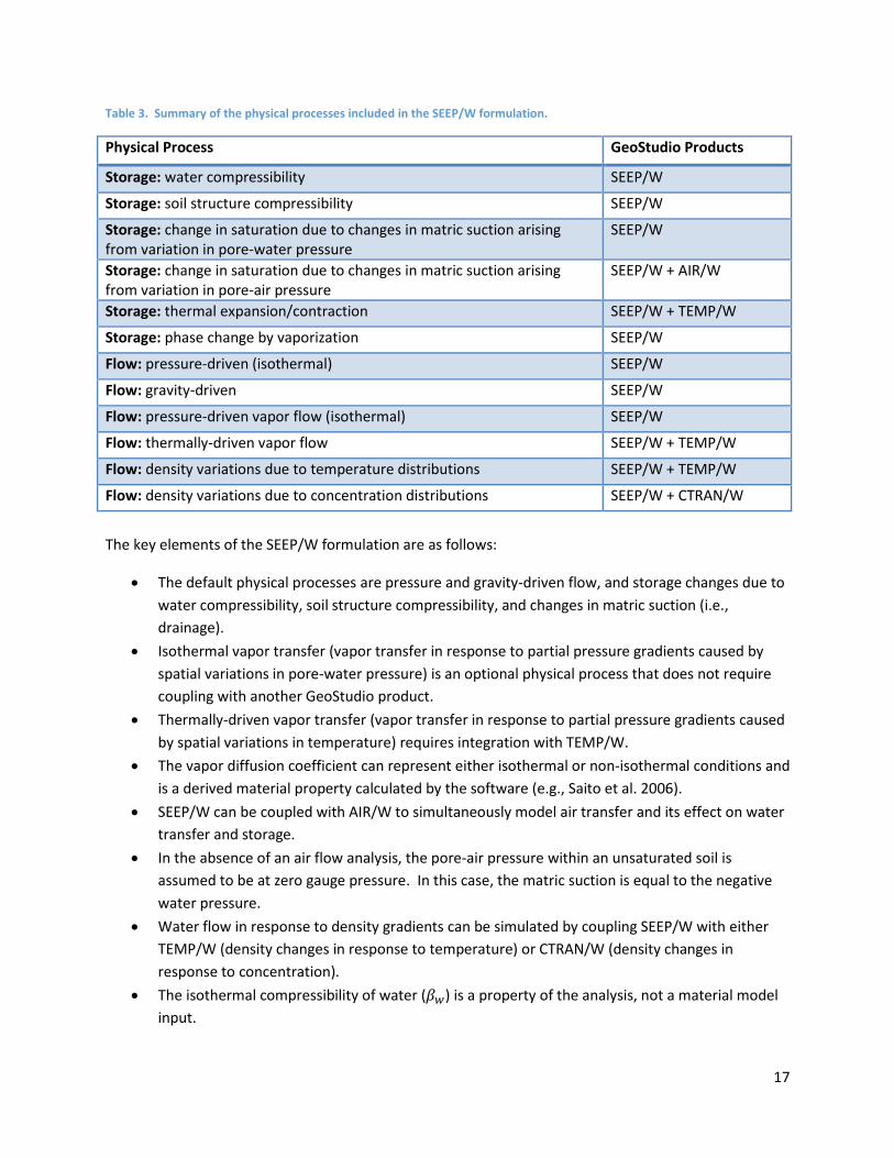
Table 3. Summary of the physical processes included in the SEEP/W formulation.

Physical Process GeoStudio Products

Storage: water compressibility SEEP/W

Storage: soil structure compressibility SEEP/W

Storage: change in saturation due to changes in matric suction arising from variation in pore-water pressure

SEEP/W

Storage: change in saturation due to changes in matric suction arising from variation in pore-air pressure

SEEP/W + AIR/W

Storage: thermal expansion/contraction SEEP/W + TEMP/W

Storage: phase change by vaporization SEEP/W

Flow: pressure-driven (isothermal) SEEP/W

Flow: gravity-driven SEEP/W

Flow: pressure-driven vapor flow (isothermal) SEEP/W

Flow: thermally-driven vapor flow SEEP/W + TEMP/W

Flow: density variations due to temperature distributions SEEP/W + TEMP/W

Flow: density variations due to concentration distributions SEEP/W + CTRAN/W

The key elements of the SEEP/W formulation are as follows:

The default physical processes are pressure and gravity-driven flow, and storage changes due to

water compressibility, soil structure compressibility, and changes in matric suction (i.e.,

drainage).

Isothermal vapor transfer (vapor transfer in response to partial pressure gradients caused by

spatial variations in pore-water pressure) is an optional physical process that does not require

coupling with another GeoStudio product.

Thermally-driven vapor transfer (vapor transfer in response to partial pressure gradients caused

by spatial variations in temperature) requires integration with TEMP/W.

The vapor diffusion coefficient can represent either isothermal or non-isothermal conditions and

is a derived material property calculated by the software (e.g., Saito et al. 2006).

SEEP/W can be coupled with AIR/W to simultaneously model air transfer and its effect on water

transfer and storage.

In the absence of an air flow analysis, the pore-air pressure within an unsaturated soil is

assumed to be at zero gauge pressure. In this case, the matric suction is equal to the negative

water pressure.

Water flow in response to density gradients can be simulated by coupling SEEP/W with either

TEMP/W (density changes in response to temperature) or CTRAN/W (density changes in

response to concentration).

The isothermal compressibility of water (𝛽𝑤) is a property of the analysis, not a material model

input.

18

The volumetric coefficient of thermal expansion at constant pressure (𝛼𝑤) is a property of the

analysis, not a material model input. The coefficient is calculated by the software from a

functional relationship between water density and temperature developed by the International

Committee for Weights and Measures.

The soil structure compressibility (𝛽) is a material model input.

Changes in storage due to soil structure compressibility are due solely to pore-water pressure

changes; therefore, the total stresses within the domain are assumed constant.

3.2 Material Models The material models in SEEP/W characterize the ability of a porous medium to store and transmit water.

The transmission and storage properties for vapor are calculated automatically by the software, while

the properties for liquid water are user inputs. The liquid water storage property defines the change in

the stored mass of liquid water in response to pore-water pressure variation (Equation 4). The hydraulic

conductivity function describes the ability of a soil to transmit water in response to the energy gradients

(Equation 6).

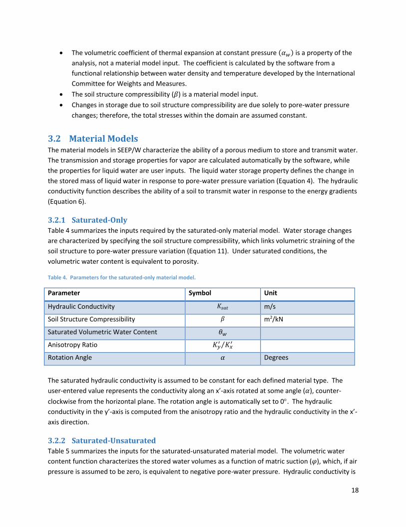
3.2.1 Saturated-Only

Table 4 summarizes the inputs required by the saturated-only material model. Water storage changes

are characterized by specifying the soil structure compressibility, which links volumetric straining of the

soil structure to pore-water pressure variation (Equation 11). Under saturated conditions, the

volumetric water content is equivalent to porosity.

Table 4. Parameters for the saturated-only material model.

Parameter Symbol Unit

Hydraulic Conductivity 𝐾𝑠𝑎𝑡 m/s

Soil Structure Compressibility 𝛽 m2/kN

Saturated Volumetric Water Content 𝜃𝑤

Anisotropy Ratio 𝐾𝑦′ 𝐾𝑥

′⁄

Rotation Angle 𝛼 Degrees

The saturated hydraulic conductivity is assumed to be constant for each defined material type. The

user-entered value represents the conductivity along an x’-axis rotated at some angle (𝛼), counter-

clockwise from the horizontal plane. The rotation angle is automatically set to 0. The hydraulic

conductivity in the y’-axis is computed from the anisotropy ratio and the hydraulic conductivity in the x’-

axis direction.

3.2.2 Saturated-Unsaturated

Table 5 summarizes the inputs for the saturated-unsaturated material model. The volumetric water

content function characterizes the stored water volumes as a function of matric suction (𝜑), which, if air

pressure is assumed to be zero, is equivalent to negative pore-water pressure. Hydraulic conductivity is

19

a function of the volumetric water content, and therefore indirectly a function of pore-water pressure.

Figure 1 presents an example of both functions.

Table 5. Parameters for the saturated-unsaturated material model.


Hydraulic Conductivity Function 𝐾(𝑢𝑤) m/s

Soil Structure Compressibility 𝛽 m2/kN (1/kPa)

Volumetric Water Content Function 𝜃𝑤(𝑢𝑤)

Anisotropy Ratio 𝐾𝑦′ 𝐾𝑥

′⁄

Rotation Angle 𝛼 Degrees

Figure 1. Examples of (a) volumetric water content and (b) hydraulic conductivity functions.

3.2.2.1 Hydraulic Conductivity of Frozen Ground

If SEEP/W is coupled to the thermal analyses product (TEMP/W), there is an option to reduce the

hydraulic conductivity of the saturated-unsaturated material model when the soil freezes. The change

in water pressure within the liquid water of a partially frozen soil can be determined from the Clapeyron

thermodynamic equilibrium equation (Schofield, 1935; Williams and Smith, 1989):

𝜕𝑢𝑤

𝜕𝑇=

ℎ𝑠𝑓

𝑣𝑤𝑇0

Equation 12

where 𝜕𝑇 is the change in temperature below the phase change temperature, ℎ𝑠𝑓 is the latent heat of

vaporization, 𝑣𝑤 is the specific volume of water, and 𝑇0 is the normal freezing point of water at

atmospheric pressure. Equation 12 is used to calculate the reduction in pore-water pressure of the

unfrozen liquid water, which is then used to determine the conductivity directly from the hydraulic

conductivity function.

VWC Function

Vo

l. W

ate

r C

on

ten

t (m

³/m

³)

Negative Pore-Water Pressure (kPa)

0

0.05

0.1

0.15

0.2

0.25

0.3

0.35

0.4

0.45

0.01 10000.1 1 10 100

K-Function

X-C

on

du

cti

vit

y (

m/s

ec

)

Matric Suction (kPa)

1.0e-05

1.0e-13

1.0e-12

1.0e-11

1.0e-10

1.0e-09

1.0e-08

1.0e-07

1.0e-06

0.01 10000.1 1 10 100

(a) (b)

20

3.2.3 Estimation Techniques

3.2.3.1 Volumetric Water Content Function

GeoStudio provides a number of methods for estimating the volumetric water content function. Closed

form equations requiring curve fit parameters can be used to generate the volumetric water content

function according to techniques developed by Fredlund and Xing (1994):

𝜃𝑤 = 𝐶(𝜑)𝜃𝑠𝑎𝑡

𝑙𝑛 [𝑒 + (𝜑𝑎

)𝑛

]𝑚

Equation 13

or van Genuchten (1980):

𝜃𝑤 = 𝜃𝑟𝑒𝑠 +𝜃𝑠𝑎𝑡 − 𝜃𝑟𝑒𝑠

[1 + (𝑎′𝜑)𝑛]𝑚

Equation 14

where 𝑎, 𝑎′, 𝑛, and 𝑚 are curve fitting parameters that control the shape of the volumetric water

content function, 𝐶(𝜑) is a correlation function, 𝜃𝑠𝑎𝑡 is the saturated volumetric water content, and 𝜃𝑟𝑒𝑠

is the residual volumetric water content. Note that the parameter 𝑎 in Equation 13 has units of pressure

and is related to the parameter 𝑎′ (𝑎′ = 1/𝑎), used by van Genuchten (1980) in Equation 14.

Sample volumetric water content functions are available for a variety of soil particle size distributions,

ranging from clay to gravel. These sample functions are generated by using characteristic curve fit

parameters in Equation 14. The volumetric water content function can also be estimated using the

modified Kovacs model developed by Aubertin et al. (2003). The model requires grain size data

including the diameter corresponding to 10% and 60% passing on the grain size curve (i.e., D10 and D60),

and the liquid limit. Finally, tabular data for volumetric water content and suction, obtained from the

literature, estimated from other pedotransfer functions or from the results of laboratory testing, can be

entered directly into the model.

3.2.3.2 Hydraulic Conductivity Function

GeoStudio provides two routines to estimate the hydraulic conductivity function from the saturated

hydraulic conductivity and the volumetric water content function. The first is the Fredlund and Xing

(1994) equation:

𝐾𝑤(𝜃𝑤) = 𝐾𝑠𝑎𝑡 ∫𝜃𝑤 − 𝑥

𝜑2(𝑥)𝑑𝑥

𝜃𝑤

𝜃𝑟𝑒𝑠

∫𝜃𝑠𝑎𝑡 − 𝑥

𝜑2(𝑥)𝑑𝑥

𝜃𝑠𝑎𝑡

𝜃𝑟𝑒𝑠

⁄ Equation 15

where 𝐾𝑠𝑎𝑡 is the saturated hydraulic conductivity, 𝑥 is a dummy variable of integration representing the

water content, and the remainder of the symbols are defined in Section 3.2.3.1.

The second estimation method is the equation proposed by van Genuchten (1980). The parameters in

the equation are generated using the curve fitting parameters from the volumetric water content

function and an input value for saturated hydraulic conductivity. The closed-form equation for hydraulic

conductivity is as follows:

21

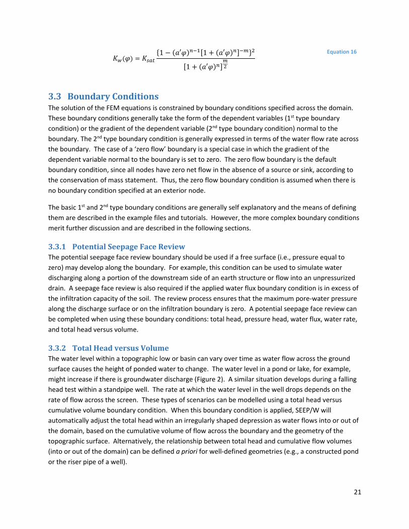
𝐾𝑤(𝜑) = 𝐾𝑠𝑎𝑡

{1 − (𝑎′𝜑)𝑛−1[1 + (𝑎′𝜑)𝑛]−𝑚}2

[1 + (𝑎′𝜑)𝑛]𝑚2

Equation 16

3.3 Boundary Conditions The solution of the FEM equations is constrained by boundary conditions specified across the domain.

These boundary conditions generally take the form of the dependent variables (1st type boundary

condition) or the gradient of the dependent variable (2nd type boundary condition) normal to the

boundary. The 2nd type boundary condition is generally expressed in terms of the water flow rate across

the boundary. The case of a ‘zero flow’ boundary is a special case in which the gradient of the

dependent variable normal to the boundary is set to zero. The zero flow boundary is the default

boundary condition, since all nodes have zero net flow in the absence of a source or sink, according to

the conservation of mass statement. Thus, the zero flow boundary condition is assumed when there is

no boundary condition specified at an exterior node.

The basic 1st and 2nd type boundary conditions are generally self explanatory and the means of defining

them are described in the example files and tutorials. However, the more complex boundary conditions

merit further discussion and are described in the following sections.

3.3.1 Potential Seepage Face Review

The potential seepage face review boundary should be used if a free surface (i.e., pressure equal to

zero) may develop along the boundary. For example, this condition can be used to simulate water

discharging along a portion of the downstream side of an earth structure or flow into an unpressurized

drain. A seepage face review is also required if the applied water flux boundary condition is in excess of

the infiltration capacity of the soil. The review process ensures that the maximum pore-water pressure

along the discharge surface or on the infiltration boundary is zero. A potential seepage face review can

be completed when using these boundary conditions: total head, pressure head, water flux, water rate,

and total head versus volume.

3.3.2 Total Head versus Volume

The water level within a topographic low or basin can vary over time as water flow across the ground

surface causes the height of ponded water to change. The water level in a pond or lake, for example,

might increase if there is groundwater discharge (Figure 2). A similar situation develops during a falling

head test within a standpipe well. The rate at which the water level in the well drops depends on the

rate of flow across the screen. These types of scenarios can be modelled using a total head versus

cumulative volume boundary condition. When this boundary condition is applied, SEEP/W will

automatically adjust the total head within an irregularly shaped depression as water flows into or out of

the domain, based on the cumulative volume of flow across the boundary and the geometry of the

topographic surface. Alternatively, the relationship between total head and cumulative flow volumes

(into or out of the domain) can be defined a priori for well-defined geometries (e.g., a constructed pond

or the riser pipe of a well).

22

Figure 2. Example of the Total Head versus Volume boundary condition applied to the inside of an excavation.

3.3.3 Unit Gradient

Water that enters the ground surface and passes beyond an upper active zone to enter the deeper

groundwater system is considered recharge or deep/net percolation. In uniform, deep, unsaturated

zones, the gravity gradient becomes the dominant gradient responsible for net percolation. In this

situation, the hydraulic gradient is equal to the elevation gradient (𝑑𝑦/𝑑𝑦), which is always 1.0. Since

the vertical hydraulic gradient produced by gravity is unity, the rate of net percolation and the hydraulic

conductivity become numerically equal and the pore-water pressures remain relatively constant with

depth. Under these conditions, Darcy’s Law can be written as follows (after Equation 6):

𝑞𝑤 = −𝐾𝑤 (𝜕𝑢𝑤

𝜕𝑦+

𝜕𝑦

𝜕𝑦) = −𝐾𝑤(0.0 + 1.0) = −𝐾𝑤

Equation 17

The unit gradient boundary condition can be applied to the lower boundary of a domain when the

negative pore-water pressure (suction) is assumed to be constant with depth. However, this

assumption does not require that suction is constant with time because a change in the flux rate

associated with net percolation will affect suction even under the unit gradient conditions.

3.3.4 Land-Climate Interaction

SEEP/W can simulate Soil-Vegetation-Atmosphere-Transfers across the ground surface using the land-

climate interaction (LCI) boundary condition. The LCI boundary condition can reflect various ground

surface conditions including bare, snow-covered, or vegetated ground. A boundary condition of this

type can be used to compute the water balance and net percolation through an engineered cover

system or evaluate the ability of a cover system to provide sufficient water for long-term plant growth.

3.3.4.1 Surface Mass Balance Equation

The water flux at the ground surface can be calculated with a mass balance equation:

(𝑞𝑃 + 𝑞𝑀)𝑐𝑜𝑠𝛼 + 𝑞𝐸 + 𝑞𝑅 = 𝑞𝐼 Equation 18

23

where superscripts on the water fluxes (𝑞) indicate rainfall (𝑃), snow melt (𝑀), infiltration (𝐼),

evaporation (𝐸) and runoff (𝑅), and 𝛼 is the slope angle. The slope angle is used to convert vertical flux

rates (i.e., P and M) to fluxes normal to the boundary. The evaporation and runoff fluxes are negative;

that is, out of the domain. Infiltration is the residual of the mass balance equation and forms the

boundary condition of the water transfer equation. Transpiration does not appear in Equation 18

because root water uptake occurs below the ground surface.

If the applied infiltration flux results in ponding, the pore-water pressure is set to zero and the time step

is resolved. Runoff is then calculated at the end of the time step as:

𝑞𝑅 = 𝑞𝐼𝑠𝑖𝑚 − (𝑞𝑃 + 𝑞𝑀)𝑐𝑜𝑠𝛼 − 𝑞𝐸 Equation 19

where 𝑞𝐼𝑠𝑖𝑚 is the simulated infiltration flux.

The maximum amount of evapotranspiration at a site is defined by the potential evapotranspiration

(PET). This potential rate of water transfer is partitioned into potential evaporation (PE) and potential

transpiration (PT) based on the soil cover fraction (SCF). SCF varies from 0.0 for bare ground to 1.0 for a

heavily vegetated surface. The proportion of PET attributed to potential surface evaporation is:

𝑞𝑃𝐸 = 𝑞𝑃𝐸𝑇(1 − 𝑆𝐶𝐹) Equation 20

while the portion that is potential transpiration flux is:

𝑞𝑃𝑇 = 𝑞𝑃𝐸𝑇(𝑆𝐶𝐹) Equation 21

Equation 21 is used to calculate root water uptake. The evaporation flux at the ground surface rarely

equals the potential evaporation due to limited water availability. The evaporation flux in Equation 18 is

calculated by recasting Equation 20 as:

𝑞𝐸 = 𝑞𝐴𝐸(1 − 𝑆𝐶𝐹) Equation 22

where 𝑞𝐴𝐸 is the actual evaporation.

Ritchie (1972) proposed the following equation, based on the interception of solar radiation by the

vegetation canopy, to apportion PET into PE and PT:

𝑆𝐶𝐹 = 1 − 𝑒−𝑘(𝐿𝐴𝐼) Equation 23

where 𝐿𝐴𝐼 is the leaf area index and 𝑘 is a constant governing the radiation extinction by the canopy as

a function of the sun angle, distribution of plants, and arrangement of leaves. The value of 𝑘 is generally

between 0.5 and 0.75. Various expressions exist for estimating 𝐿𝐴𝐼 from crop height.

3.3.4.1.1 Calculation of Evapotranspiration

Modelling evaporative flux at the ground surface (Equation 19 and Equation 22) requires knowledge of

the actual evaporation, while modelling root water uptake via Equation 21 requires the potential

24

evapotranspiration. There are three ‘Evapotranspiration’ methods available in SEEP/W: 1) user-defined;

2) Penman-Wilson; and, 3) Penman-Monteith.

The potential evapotranspiration is specified as a function of time for method 1. The actual evaporation

is calculated using the relationship proposed by Wilson et al. (1997):

𝑞𝐴𝐸 = 𝑞𝑃𝐸𝑇 [𝑝𝑣

𝑠 − 𝑝𝑣𝑎

𝑝𝑣0𝑠 − 𝑝𝑣

𝑎] Equation 24

where 𝑝𝑣𝑠 and 𝑝𝑣

𝑎 are the vapor pressures at the surface of the soil and the air above the soil,

respectively, and 𝑝𝑣0𝑠 is the vapor pressure at the surface of the soil for the saturated condition (kPa).

The term in brackets, which is referred to as the limiting function (𝐿𝐹), is a ratio of the actual vapor

pressure deficit to the potential vapor pressure deficit for a fully saturated soil. The user input, 𝑞𝑃𝐸𝑇,

can be determined from measured data or empirical and semi-empirical methods such as Thornthwaite

(1948) and Penman (1948).

The second method, the Penman-Wilson method, is based on the modification of the well-known

Penman (1948) equation used to calculate potential evaporation. The Penman-Wilson method

calculates the actual evaporation from the bare ground surface as (Wilson et al., 1997):

𝑞𝐴𝐸 =Γ𝑞𝑛

∗ + 𝛾𝐸𝑎

Γ + 𝛾/ℎ𝑠

Equation 25

where the aridity, 𝐸𝑎, is given as:

𝐸𝑎 = [2.625(1 + 0.146𝑢)]𝑝𝑣𝑎 (1

ℎ𝑎⁄ − 1

ℎ𝑠⁄ ) Equation 26

and

ℎ𝑎 Relative humidity of the air ℎ𝑠 Relative humidity of the soil Γ Slope of the saturation vapor pressure verses temperature curve

𝑞𝑛∗ Net radiation in terms of water flux

𝛾 Psychrometric constant = 0.0665 kPa/C 𝑢 Wind speed

The Penman-Wilson equation calculates potential evapotranspiration by substituting a relative humidity

of 1.0 into Equation 25, which causes the equation to revert to the original Penman equation (Penman,

1948). Calculation of the relative humidity at the ground surface (ℎ𝑠) requires temperature and matric

suction. A heat transfer analysis (TEMP/W) can be used to compute the temperature at the ground

surface; otherwise, the ground temperature is assumed to be equal to the air temperature.

Monteith extended the original work of Penman to crop surfaces by introducing resistance factors. The

Penman-Monteith equation (method 3) for calculating potential evapotranspiration, 𝑞𝑃𝐸𝑇, is well

accepted in the soil science and agronomy fields and is the recommended procedure of the Food and

Agriculture Organization of the United Nations (Allen et al., 1998). This method is generally best for

25

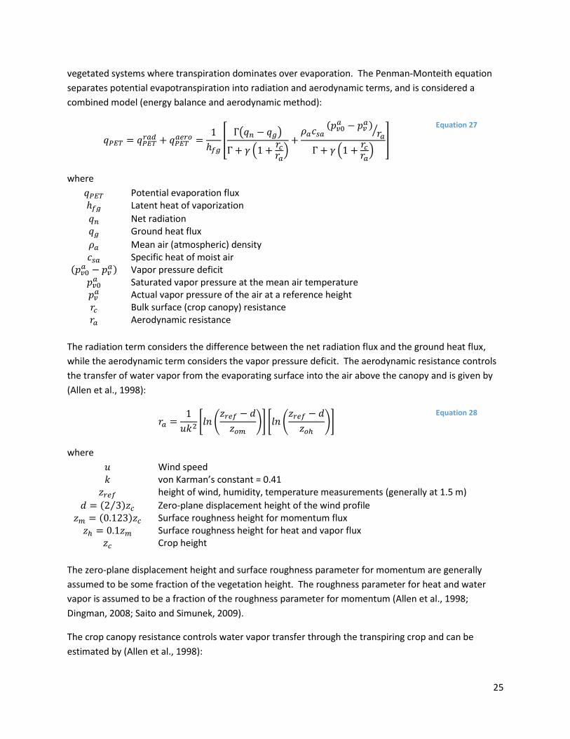
vegetated systems where transpiration dominates over evaporation. The Penman-Monteith equation

separates potential evapotranspiration into radiation and aerodynamic terms, and is considered a

combined model (energy balance and aerodynamic method):

𝑞𝑃𝐸𝑇 = 𝑞𝑃𝐸𝑇𝑟𝑎𝑑 + 𝑞𝑃𝐸𝑇

𝑎𝑒𝑟𝑜 =1

ℎ𝑓𝑔[

Γ(𝑞𝑛 − 𝑞𝑔)

Γ + 𝛾 (1 +𝑟𝑐𝑟𝑎

)+

𝜌𝑎𝑐𝑠𝑎(𝑝𝑣0

𝑎 − 𝑝𝑣𝑎)

𝑟𝑎⁄

Γ + 𝛾 (1 +𝑟𝑐𝑟𝑎

)]

Equation 27

where

𝑞𝑃𝐸𝑇 Potential evaporation flux ℎ𝑓𝑔 Latent heat of vaporization

𝑞𝑛 Net radiation 𝑞𝑔 Ground heat flux

𝜌𝑎 Mean air (atmospheric) density 𝑐𝑠𝑎 Specific heat of moist air

(𝑝𝑣0𝑎 − 𝑝𝑣

𝑎) Vapor pressure deficit 𝑝𝑣0

𝑎 Saturated vapor pressure at the mean air temperature

𝑝𝑣𝑎 Actual vapor pressure of the air at a reference height

𝑟𝑐 Bulk surface (crop canopy) resistance 𝑟𝑎 Aerodynamic resistance

The radiation term considers the difference between the net radiation flux and the ground heat flux,

while the aerodynamic term considers the vapor pressure deficit. The aerodynamic resistance controls

the transfer of water vapor from the evaporating surface into the air above the canopy and is given by

(Allen et al., 1998):

𝑟𝑎 =1

𝑢𝑘2[𝑙𝑛 (

𝑧𝑟𝑒𝑓 − 𝑑

𝑧𝑜𝑚)] [𝑙𝑛 (

𝑧𝑟𝑒𝑓 − 𝑑

𝑧𝑜ℎ)]

Equation 28

where

𝑢 Wind speed 𝑘 von Karman’s constant = 0.41

𝑧𝑟𝑒𝑓 height of wind, humidity, temperature measurements (generally at 1.5 m)

𝑑 = (2 3⁄ )𝑧𝑐 Zero-plane displacement height of the wind profile 𝑧𝑚 = (0.123)𝑧𝑐 Surface roughness height for momentum flux

𝑧ℎ = 0.1𝑧𝑚 Surface roughness height for heat and vapor flux 𝑧𝑐 Crop height

The zero-plane displacement height and surface roughness parameter for momentum are generally

assumed to be some fraction of the vegetation height. The roughness parameter for heat and water

vapor is assumed to be a fraction of the roughness parameter for momentum (Allen et al., 1998;

Dingman, 2008; Saito and Simunek, 2009).

The crop canopy resistance controls water vapor transfer through the transpiring crop and can be

estimated by (Allen et al., 1998):

26

𝑟𝑐 =𝑟𝑙

0.5𝐿𝐴𝐼=

100

0.5𝐿𝐴𝐼=

200

𝐿𝐴𝐼

Equation 29

where 𝑟𝑙 is bulk stomatal resistance of the well-illuminated leaf. The 𝐿𝐴𝐼 cannot be zero (bare ground)

in Equation 29, so a minimum of 0.1 is imposed in SEEP/W.

Potential evapotranspiration is calculated for a vegetated surface of any height. The potential

evapotranspiration value is then apportioned into evaporative and transpiration fluxes, using Equation

20 and Equation 21. As such, method 3 does not reduce PE to AE based on water availability. It is worth

noting that the crop canopy resistance approaches infinity as the 𝐿𝐴𝐼 approaches zero. Thus, the

Penman-Monteith equation does not adequately represent evaporation-dominant systems.

3.3.4.1.2 Root Water Uptake

SEEP/W determines the root water uptake as part of the LCI boundary condition if vegetation

characteristics have been defined. A general equation for the maximum possible root water extraction

rate per volume of soil, 𝑞𝑟𝑜𝑜𝑡𝑚𝑎𝑥, over a root zone of arbitrary shape is given by (Feddes et al., 2001):

𝑞𝑟𝑜𝑜𝑡 = 𝜋𝑟𝑜𝑜𝑡′ 𝛼𝑟𝑤𝑞𝑃𝑇 Equation 30

where 𝛼𝑟𝑤 is a reduction factor due to water stress, 𝑞𝑃𝑇 is equal to the potential transpiration flux, and

𝜋𝑟𝑜𝑜𝑡′ is the normalized water uptake distribution. The potential transpiration flux is computed using

Equation 21. The reduction factor is defined by a plant limiting function, which is a functional

relationship between the reduction factor and matric suction. Equation 30 is uniquely calculated at

each gauss point within the root zone.

The normalized water uptake distribution is:

𝜋𝑟𝑜𝑜𝑡′ =

𝜋𝑟𝑜𝑜𝑡

∫ 𝜋𝑟𝑜𝑜𝑡𝑟𝑚𝑎𝑥

0𝑑𝑟

Equation 31

where 𝜋𝑟𝑜𝑜𝑡 is the root length density or the length of root per volume of soil. Integration of the root

density function over the maximum root depth, 𝑟𝑚𝑎𝑥, gives the total root length beneath a unit area.

Normalizing the uptake distribution ensures that the normalized water uptake distribution is unity over

the maximum root depth:

∫ 𝜋𝑟𝑜𝑜𝑡′

𝑟𝑚𝑎𝑥

0

𝑑𝑟 = 1.0 Equation 32

Finally, integration of Equation 30 over the rooting depth recovers the actual transpiration flux:

𝑞𝐴𝑇 = ∫ 𝑞𝑟𝑜𝑜𝑡

𝑟𝑚𝑎𝑥

0

𝑑𝑟 Equation 33

27

3.3.4.1.3 Snow Melt

The LCI boundary condition in SEEP/W calculates the water flux associated with snowmelt (in Equation

18) based on the change in snow pack depth between time steps:

𝑞𝑀 =∆ℎ𝑠𝑛𝑜𝑤

∆𝑡

𝜌𝑠𝑛𝑜𝑤

𝜌𝑤

Equation 34

where ∆ℎ𝑠𝑛𝑜𝑤 is the change in snow depth, ∆𝑡 is the time increment, and 𝜌𝑠𝑛𝑜𝑤 is the snow density. A

snow depth verses time function is required to calculate snowmelt flux. Snow depth data can be

measured or estimated using a temperature-index method (see examples).

3.3.4.2 Inputs

Table 6 presents the LCI inputs for the three different evapotranspiration methods. All three methods

require functions for air temperature, precipitation, and relative humidity over time. Snow depth and

snow density are optional, although the later must be defined if snowmelt is to be modelled. The

Penman-Wilson and Penman-Monteith equations require wind speed and net radiation. SEEP/W

provides an option to select solar radiation (incoming) so that net radiation is calculated during solve-

time (see Section 4.3.1). The Penman-Monteith equation requires vegetation height. Finally, the user-

defined option requires that potential evapotranspiration is specified over time.

Table 6. Inputs for the land-climate interaction boundary condition.

Evapotranspiration Method Inputs

All Air temperature versus time Precipitation flux versus time Relative humidity Snow depth versus time (optional) Snow density (optional)

Penman-Wilson & Penman-Monteith Wind speed versus time Net radiation versus time

Penman-Monteith Vegetation height versus time

User-Defined Potential evapotranspiration verses time

Table 7 presents the vegetation data inputs required for modelling root water uptake. All

evapotranspiration methods require inputs for leaf area index, plant moisture limiting, root depth,

normalized root density, and soil cover fraction.

Table 7. Inputs for root water uptake.

Evapotranspiration Method Inputs

All Leaf area index versus time Plant moisture limiting function Root depth versus time function Normalized root density Soil cover fraction versus time function

28

3.3.5 Diurnal Distributions

3.3.5.1 Air Temperature

The air temperature at any hour of the day can be estimated from the daily maximum and minimum

values with:

𝑇𝑎 =𝑇𝑚𝑎𝑥 + 𝑇𝑚𝑖𝑛

2+

𝑇𝑚𝑎𝑥 − 𝑇𝑚𝑖𝑛

2𝑐𝑜𝑠 [2𝜋 (

𝑡 − 13

24)]

Equation 35

where 𝑇𝑚𝑎𝑥 and 𝑇𝑚𝑖𝑛 are the daily maximum and minimum temperatures, respectively, and 𝑡 is the

time in hours since 00:00:00. The approximation, which is used by Šimůnek et al. (2012) and presented

by Fredlund et al. (2012), assumes the lowest and highest temperature to occur at 01:00 and 13:00,

respectively. Equation 35 provides a continuous variation of the air temperature throughout the day;

however, the diurnal distributions are discontinuous from day-to-day. A continuous function over

multiple days is obtained by calculating 𝑇𝑎 for 𝑡 > 13: 00 using 𝑇𝑚𝑖𝑛 from the subsequent day.

3.3.5.2 Relative Humidity

The relative humidity at any hour of the day can be estimated from the measured daily maximum and

minimum values in the air:

ℎ𝑎 =ℎ𝑚𝑎𝑥 + ℎ𝑚𝑖𝑛

2+

ℎ𝑚𝑎𝑥 − ℎ𝑚𝑖𝑛

2𝑐𝑜𝑠 [2𝜋 (

𝑡 − 1

24)]

Equation 36

where ℎ𝑚𝑎𝑥 and ℎ𝑚𝑖𝑛 are the daily maximum and minimum relative humidity, respectively, and 𝑡 is the

time in hours since 00:00:00. The approximation, which is used by Šimůnek et al. (2012) and presented

by Fredlund et al. (2012), assumes the lowest and highest relative humidity to occur at 13:00 and 01:00,

respectively, which are the opposite times as the air temperature peaks. Equation 36 provides

continuous variation of the relative humidity throughout the day; however, the diurnal distributions are

discontinuous from day-to-day. Similar to the temperature function, the relative humidity function is

continuous over multiple days if ℎ𝑎 for 𝑡 > 13: 00 is calculated with ℎ𝑚𝑎𝑥 from the subsequent day.

3.3.5.3 Daily Potential Evapotranspiration

User-defined daily PET values can be distributed across the day in accordance with diurnal variations in

net radiation. Fayer (2000) assumes the fluxes are constant between about 0 to 6 hours and 18 to 24

hours, and otherwise follow a sinusoidal distribution:

𝑞𝑃𝐸𝑇 = 0.24(𝑞𝑃𝐸𝑇 ) 𝑡 < 0.264 𝑑; 𝑡 > 0.736 𝑑 Equation 37

and

𝑞𝑃𝐸𝑇 = 2.75(𝑞𝑃𝐸𝑇 )𝑠𝑖𝑛 (2𝜋𝑡 −𝜋

2) 0.264 𝑑 ≤ 𝑡 ≤ 0.736 𝑑 Equation 38

29

where the daily average potential evapotranspiration flux, 𝑞𝑃𝐸𝑇 , is expressed with the same time units

as the time variable. Equation 37 and Equation 38 produce a continuous function of instantaneous flux.

A finite element formulation is discretized in time and assumes the flux constant over the time step.

GeoStudio therefore obtains the potential evaporation flux by numerically integrating the function

between the beginning and end of the step and dividing by the time increment.


3.3.6.1 Snow Depth

Snow depth on the ground surface at any instant in time, ℎ𝑠𝑛𝑜𝑤, is the summation of all incremental

snow depth accumulations minus snowmelt:

ℎ𝑠𝑛𝑜𝑤 = ∑(∆ℎ𝑠𝑛𝑜𝑤 − ∆ℎ𝑚𝑒𝑙𝑡)

𝑡

0

Equation 39

where ∆ℎ𝑠𝑛𝑜𝑤 is the incremental snow depth accumulation corrected for ablation and ∆ℎ𝑚𝑒𝑙𝑡

represents the snowmelt over a given period.

Snow accumulation models often use temperature near the ground surface to determine the fraction of

precipitation falling as rain or snow (e.g., SNOW-17, Anderson, 2006). SEEP/W sets the fraction of

precipitation occurring as snow, 𝑓𝑠, to 1.0 if the average air temperature over the time interval is less

than or equal to the specified threshold temperature. Conversely, the snow fraction is set to 0.0 if the

average air temperature over the time interval was greater than the threshold value. The threshold

temperature is a model input.

Snow accumulation over the time interval in terms of snow-water equivalent, ∆ℎ𝑠𝑤𝑒, is determined by:

∆ℎ𝑠𝑤𝑒 = ℎ𝑃 × 𝑓𝑠 × 𝑀𝐹 Equation 40

where ℎ𝑃 is the precipitation depth (liquid) over the time interval, and 𝑀𝐹 is a multiplier factor

determined from the ablation constant as:

𝑀𝐹 = 1 − 𝐴𝑏𝑙𝑎𝑡𝑖𝑜𝑛 𝐶𝑜𝑛𝑠𝑡𝑎𝑛𝑡 Equation 41

The snow depth accumulated over the interval is then calculated as:

∆ℎ𝑠𝑛𝑜𝑤 = ∆ℎ𝑠𝑤𝑒

𝜌𝑤

𝜌𝑠𝑛𝑜𝑤

Equation 42

where the snow density, 𝜌𝑠𝑛𝑜𝑤, is input as a model parameter.

Snowmelt is assumed to only occur when the average air temperature is greater than 0ᵒC. The daily

snow melt depth, a model input, is used to compute snowmelt rate for a given time interval.

30

3.4 Convergence

3.4.1 Water Balance Error

The transient water transfer equation is formulated from the principle of mass conservation. As such,

an apparent water balance error can be calculated by comparing the cumulative change in stored mass

to the cumulative mass of water that flowed past the domain boundaries. The error is ‘apparent’

because it is a mathematical by-product of non-convergence, not an actual loss of mass, since the

solution conserves mass.

The software allows for inspection of mass balance errors on sub-domains. Sub-domains are essentially

control volumes that comprise a group of elements. The elements undergo changes in stored mass

during a transient analysis. Water enters or exits the sub-domain at nodes on the boundary of the sub-

domain and nodes inside the domain to which boundary conditions are applied (e.g., root water

uptake).

The cumulative mass of water that enters the domain, ��𝑖𝑛, minus the mass of water that leaves the

domain, ��𝑜𝑢𝑡, plus the mass of water that is added to (or removed from) the domain, ��𝑆, can be

calculated by reassembling the forcing vector:

∫ (��𝑖𝑛 − ��𝑜𝑢𝑡 + ��𝑆)𝑡

0

𝑑𝑡 = ∑ ��𝑑𝑡

𝑡

0

Equation 43

The rate of increase in the mass of water stored within the domain is:

∫ ��𝑠𝑡

𝑡

0

𝑑𝑡 Equation 44

The change in stored mass (Equation 44) is calculated in accordance with the final solution and all of the

storage terms shown in Equation 9 and/or listed in Table 3 (e.g., thermal expansion of water). The

calculated mass balance error is the difference between Equation 44 and Equation 43. The relative error

is calculated by dividing the absolute error by the maximum of Equation 43 or Equation 44.

3.4.2 Conductivity Comparison

Convergence can also be assessed by comparing the input hydraulic conductivity functions to a scatter

plot of the hydraulic conductivities from the penultimate iteration and the final pore water pressures.

The points of the scatter plot will generally overlie the input hydraulic functions if the solution did not

change significantly on the last two iterations. However, discrepancies might remain if the input

functions are highly non-linear, even if the changes in pore-water pressures were negligible and the

convergence criteria were satisfied (Section I.8). Therefore, evaluating convergence of non-linear

hydraulic properties requires multiple pieces of information. In addition, a less-than-perfect match

between the scatter plot and the input functions may sometimes be acceptable in the context of the

modelling objectives or in light of other convergence criteria.

31

4 Heat Transfer with TEMP/W TEMP/W is a finite element program for simulating heat transfer through porous media. Typical

applications of TEMP/W include studies of naturally occurring frozen ground (e.g., permafrost), artificial

ground freezing (e.g., for ground stabilization or seepage control), and frost propagation (e.g., for

insulation design for structures or roadways). Section 4.1 summarizes the heat transfer and storage

processes that are included in the formulation, while Section 4.2 describes the constitutive models

available to characterize the properties of the medium and Section 4.3 describes the boundary

conditions unique to TEMP/W.

4.1 Theory The TEMP/W formulation is based on the law of energy conservation or the first law of

thermodynamics, which states that the total energy of a system is conserved unless energy crosses its

boundaries (Incropera et al., 2007). Similarly, the rate of change of stored thermal energy within a

specified volume must be equal to the difference in the rate of heat flux into and out of the volume, as

described in the following equation:

��𝑠𝑡 ≡𝑑𝐸𝑠𝑡

𝑑𝑡= ��𝑖𝑛 − ��𝑜𝑢𝑡 + ��𝑔

Equation 45

where ��𝑠𝑡 is the rate of change in the stored thermal energy, the inflow and outflow terms, ��𝑖𝑛 and

��𝑜𝑢𝑡, represent the rate of change in heat flux across the control surfaces, and ��𝑔 is a heat sink or

source within the control volume (𝑑𝑥 𝑑𝑦 𝑑𝑧).

In a porous medium containing water, the rate of change in the thermal energy stored in this volume is:

��𝑠𝑡 = ��𝑠𝑒𝑛𝑠 + ��𝑙𝑎𝑡 = ��𝑠𝑒𝑛 + ��𝑠𝑓 + ��𝑓𝑔 Equation 46

where ��𝑠𝑒𝑛𝑠 and ��𝑙𝑎𝑡 represent the rate of change in the thermal energy associated with sensible and

latent heat, respectively, in the control volume. The rate of change in the sensible energy is equal to

(e.g., Andersland and Ladanyi, 2004):

��𝑠𝑒𝑛𝑠 = 𝐶𝑝

𝜕𝑇


Equation 47

where 𝐶𝑝 is the volumetric heat capacity associated with the control volume. Volumetric heat capacity

is the summation of the product of specific heat capacity, 𝑐𝑝, mass density, 𝜌, and volumetric fraction,

𝜃, of each component in the control volume (i.e., solid particles, water, ice, and air).

The change in latent energy within the control volume could be due to fusion, ��𝑠𝑓 (conversion from

solid to liquid or liquid to solid, via freezing or melting), or due to vaporization, ��𝑓𝑔 (conversion from

liquid to gas or vice versa, via evaporation or condensation). The latent heat of fusion, ℎ𝑠𝑓, and

vaporization, ℎ𝑓𝑔, represent the amount of energy required per unit mass of substance (i.e., water) to

effect these changes in state.

32

The rate of change in the latent energy associated with fusion for water is:

��𝑠𝑓 = −ℎ𝑠𝑓

𝜕𝑀𝑖𝑐𝑒

𝜕𝑡= −𝜌𝑖𝑐𝑒ℎ𝑠𝑓

𝜕𝜃𝑖𝑐𝑒


Equation 48

where 𝑀𝑖𝑐𝑒 is the mass of ice in the control volume, 𝜃𝑖𝑐𝑒 is the volumetric ice content, and 𝜌𝑖𝑐𝑒 is the

mass density of ice.

The rate of change in the latent energy associated with vaporization is given by:

��𝑓𝑔 = ℎ𝑓𝑔

𝜕𝑀𝑣

𝜕𝑡

Equation 49

where 𝑀𝑣 is the mass of vapor in the control volume. An increase in the mass of vapor is associated

with an increase in latent energy within the control volume. Energy is released into the control volume

during condensation and is consumed from within the control volume during vaporization.

The inflow and outflow terms (��𝑖𝑛 and ��𝑜𝑢𝑡) are associated exclusively with processes occurring at the

control surfaces. TEMP/W considers heat transfer across the boundaries via heat conduction and

advection. The rate of change in energy associated with conduction is described by Fourier’s Law (e.g.,

Carslaw and Jaeger, 1986):

��𝑦 = −𝑘𝜕𝑇

𝜕𝑦𝑑𝑥𝑑𝑧

Equation 50

where 𝑘 is the thermal conductivity of the medium.

Advection occurs when water entering or leaving the control volume transports thermal energy. The

advective heat flux may be comprised of both sensible and latent energy transfers. The net rate at

which sensible thermal energy enters the control volume with the flow of liquid water, water vapor, and

(dry) air can be calculated from the respective mass flow rates, ��:

(𝜕(��𝑦𝑢𝑡(𝑦))

𝜕𝑦)

𝑠𝑒𝑛𝑠

= 𝑐𝑤

𝜕(��𝑤𝑇)

𝜕𝑦+ 𝑐𝑣

𝜕(��𝑣𝑇)

𝜕𝑦+ 𝑐𝑎

𝜕(��𝑎𝑇)

𝜕𝑦

Equation 51

where 𝑢𝑡(𝑦) is the sensible thermal energy per unit mass calculated as the product of the temperature

and specific heat, 𝑐, with subscripts indicating water, vapor, and air.

Transport of vapor from one location to another constitutes a transport of energy in latent form

because evaporation or condensation within soil liberates or consumes heat energy (Jury and Horton,

2004). The rate of change in the latent energy due to vapor transfer into the control volume can be

computed by:

(𝜕(��𝑦𝑢𝑡(𝑦))

𝜕𝑦)

𝑙𝑎𝑡

= ℎ𝑓𝑔

𝜕��𝑣

𝜕𝑦

Equation 52

33

where ��𝑣 represents the mass flow rate of water vapor entering the control volume.

Substitution and expansion of the foregoing rate equations into the conservation statement and division

by the dimensions of the control volume gives:

(𝐶𝑝 + 𝜌𝑤ℎ𝑠𝑓

𝜕𝜃𝑢𝑤𝑐

𝜕𝑇)

𝜕𝑇

𝜕𝑡+ ℎ𝑓𝑔

𝜕𝑀𝑣

𝜕𝑡

=𝜕

𝜕𝑦(𝑘

𝜕𝑇

𝜕𝑦) − 𝑐𝑤

𝜕(��𝑤" 𝑇)

𝜕𝑦− 𝑐𝑣

𝜕(��𝑣" 𝑇)

𝜕𝑦− 𝑐𝑎

𝜕(��𝑎" 𝑇)

𝜕𝑦− ℎ𝑓𝑔

𝜕��𝑣"

𝜕𝑦

Equation 53

where the double prime indicates mass fluxes and 𝜃𝑢𝑤𝑐 is the unfrozen volumetric water content and

the apparent volumetric heat capacity, 𝐶𝑎𝑝 , is defined as:

𝐶𝑎𝑝 = 𝐶𝑝 + 𝜌𝑤ℎ𝑠𝑓

𝜕𝜃𝑢𝑤𝑐

𝜕𝑇

Equation 54

Equation 53 can be simplified by ignoring forced-convection heat transfer and the latent heat of

vaporization, giving:

𝐶𝑎𝑝

𝜕𝑇

𝜕𝑡=

𝜕

𝜕𝑦(𝑘

𝜕𝑇

𝜕𝑦)

Equation 55

Table 8 provides a complete list of the physical processes included in the partial differential equation

solved by TEMP/W.

Table 8. Summary of the physical processes included in the TEMP/W formulation.


Storage: sensible energy TEMP/W

Storage: latent heat of fusion (freeze/thaw) TEMP/W

Storage: latent heat of vaporization (vaporization/condensation) TEMP/W + SEEP/W

Flow: conduction TEMP/W

Flow: sensible heat advection with water transfer TEMP/W + SEEP/W

Flow: sensible heat advection with vapor transfer TEMP/W + SEEP/W

Flow: sensible heat advection with air transfer TEMP/W + SEEP/W + AIR/W

Flow: net latent energy transfer TEMP/W + SEEP/W

The key elements of the TEMP/W formulation are as follows:

The default physical processes in TEMP/W include conduction heat transfer and changes in

stored sensible energy and latent heat of fusion.

34

Advection heat transfer with flowing water and air – also referred to as forced convection – can

be simulated by coupling TEMP/W with SEEP/W and AIR/W, respectively.

A SEEP/W analysis that includes vapor transfer is required to evaluate the effects of vapor on

heat transfer.

The latent heat of vaporization, ℎ𝑠𝑓, and temperature at which phase change occurs are

properties of the analysis, not a material model input.

4.2 Material Models The TEMP/W material models characterize the ability of a porous medium to store and transmit heat.

The soil storage property quantifies the change in sensible energy, ��𝑠𝑒𝑛𝑠, in response to changes in

temperature and changes in the amount of latent energy associated with fusion, ��𝑠𝑓. The thermal

conductivity represents the ability of the porous medium to transmit heat in response to the

temperature gradients (Equation 50).

4.2.1 Full Thermal

Table 9 summarizes the inputs required by the full thermal material model. Changes in sensible energy

are characterized by volumetric heat capacity parameters for the unfrozen and frozen states, and the in

situ volumetric water content. Thermal conductivity is a function of temperature, so it is indirectly a

function of the portion of ice within the pore space (e.g., Andersland and Ladanyi, 2004).

Table 9. Parameters for the full thermal material model.


Thermal Conductivity function 𝑘(𝑇) J/s/m/K (W/m/K)

Volume Heat Capacity: Unfrozen 𝐶𝑝 J/m3/K

Volume Heat Capacity: Frozen 𝐶𝑝 J/m3/K

Normalized Unfrozen Volumetric Water Content function

𝜃′𝑢𝑤𝑐 =

𝜃𝑢𝑤𝑐

𝑛(𝑇)

In situ Volumetric Water Content 𝜃𝑤 = 𝑛

The normalized unfrozen volumetric water content, 𝜃′𝑢𝑤𝑐, is a function of temperature (Figure 3; e.g.,

Spaans and Baker, 1996; Flerchinger et al., 2006; Andersland and Ladanyi, 2004). This functional

relationship controls the rate of change in the latent energy of fusion per degree temperature change,

according to the second term on the left side of Equation 53. The normalized unfrozen volumetric water

content acknowledges that water within a porous medium changes phase over a temperature range

(Figure 3; see Section 4.2.4.1).

35

Figure 3. Example of an unfrozen water content versus temperature function.

4.2.2 Simplified Thermal

Table 10 summarizes the inputs required by the simplified thermal material model. The simplified

thermal constitutive model assumes that all latent heat is released or adsorbed at a single phase change

temperature. The change in volumetric ice content required by Equation 53 is assumed equal to the

specified in situ volumetric water content.

Table 10. Parameters for the simplified thermal material model.


Thermal Conductivity: Unfrozen 𝑘 J/s/m/K

Thermal Conductivity: Frozen 𝑘 J/s/m/K

Volume Heat Capacity: Unfrozen 𝐶𝑝 J/m3/K

Volume Heat Capacity: Frozen 𝐶𝑝 J/m3/K

In situ Volumetric Water Content 𝜃𝑤

The energy storage capacity for the simplified thermal model is defined in the same manner as the full

thermal model: a volume heat capacity for both the frozen and unfrozen states. Similarly, conduction is

characterized by specifying the thermal conductivity of the medium for the frozen and unfrozen states.

4.2.3 Coupled Convective

The coupled convective thermal material model can be used when the thermal properties of a material

vary with volumetric water content. For example, this material model can be used when forced

convection (or energy advection) is also being simulated. The fundamental difference between the

coupled convective and full thermal material models is the assumption regarding volumetric water

content. A full thermal material model assumes that the volumetric water content is constant

Normalized Unf rozen VWC Versus Temperature

Un

fro

ze

n W

ate

r C

on

ten

t (m

³/m

³)

Temperature (°C)

0

0.2

0.4

0.6

0.8

1

-1-2-3-4-5 0

36

throughout the analysis, such that the frozen/unfrozen volume heat capacities are constant and the

thermal conductivity is only a function of temperature. However, in a coupled heat and water transfer

analysis, the volumetric water content within the domain is known, so the thermal properties can be

defined as a function of the volumetric water content for the unfrozen state. The practical implication

of these relationships is that the thermal properties can vary throughout the domain with changes in

volumetric water content. Table 11 summarizes the inputs required by the coupled convective model.

Table 11. Parameters for the coupled convective material model.


Thermal Conductivity 𝑘′ = 𝑘(𝜃𝑤) J/s/m/K

Volume Heat Capacity 𝐶′𝑝 = 𝐶𝑝(𝜃𝑤) J/m3/K

Normalized Unfrozen Volumetric Water Content function

𝜃′𝑢𝑤𝑐 =

𝜃𝑢𝑤𝑐

𝑛(𝑇)

The coupled convective model adjusts the thermal conductivity and volumetric heat capacity if the

temperature is below the phase change value (after Johansen, 1975). The porosity and total volumetric

water content of the soil are known from the water transfer analysis. The unfrozen volumetric water

content is calculated from the normalized function, 𝜃′𝑢𝑤𝑐, at the current temperature as:

𝜃𝑢𝑤𝑐 = 𝑛𝜃′𝑢𝑤𝑐(𝑇) Equation 56

The volumetric ice content is the difference between the unfrozen and frozen water contents as:

𝜃𝑖𝑐𝑒 = 𝜃𝑤 − 𝜃𝑢𝑤𝑐 Equation 57

The thermal conductivity of the soil in the partially frozen state, 𝑘𝑝𝑓, is calculated via linear interpolation

as:

𝑘𝑝𝑓 = 𝑘′ +𝜃𝑖𝑐𝑒

𝜃𝑤[𝑘𝑓 − 𝑘′]

Equation 58

where 𝑘′ is the thermal conductivity at a given volumetric water content, and 𝑘𝑤 is the thermal

conductivity of liquid water. The thermal conductivity of the soil in a completely frozen state, 𝑘𝑓, is

calculated as:

𝑘𝑓 = 𝑘𝑠(1−𝑛)𝑘𝑖𝑐𝑒

(𝜃𝑤) Equation 59

where 𝑘𝑖𝑐𝑒 is the thermal conductivity of ice and the volumetric water content, 𝜃𝑤, is equal to the

volumetric ice content, 𝜃𝑖𝑐𝑒.

37

Finally, the thermal conductivity of the solids fraction, 𝑘𝑠, is calculated assuming the soil is unfrozen:

𝑘𝑠 = [𝑘′

(𝑘𝑤)𝜃𝑤]

(1

1−𝑛)

Equation 60

The volumetric heat capacity of the soil in the partially or fully frozen state is calculated as:

𝐶𝑝𝑓 = (1 − 𝑛)𝐶𝑠 + 𝜃𝑢𝑤𝑐𝐶𝑤 + 𝜃𝑖𝑐𝑒𝐶𝑖𝑐𝑒 + 𝜃𝑎𝐶𝑎 Equation 61

The volumetric heat capacity of the solids fraction, 𝐶𝑠, is calculated assuming the soil unfrozen as:

𝐶𝑠 =1

1 − 𝑛 (𝐶′𝑝 − 𝜃𝑤𝐶𝑤 − 𝜃𝑎𝐶𝑎)

Equation 62

where 𝐶′𝑝 is the volumetric heat capacity of a soil at a given water content, 𝐶𝑤 is the volumetric heat

capacity of water, 𝐶𝑎 is the volumetric heat capacity of air, and 𝜃𝑎 is the volumetric air content.


4.2.4.1 Normalized Unfrozen Volumetric Water Content Function

Various empirical or semi-empirical methods estimate the unfrozen volumetric water content function

(e.g., Flerchinger et al., 2006; Spaans and Baker, 1996). GeoStudio provides a number of sample

functions for the normalized unfrozen volumetric water content based on a range of soil particle size

distributions (clay to gravel). These sample functions were generated by first calculating the change in

water pressure for a shift in the freezing point temperature via the Clausius–Clapeyron thermodynamic

equilibrium equation. The (negative) pore-water pressure at the freezing point temperature is then

used to obtain the corresponding volumetric water content from the sample function referred to in

Section 3.2.2.1. The volumetric water content is then normalized by the soil porosity and cross-plotted

against the freezing point temperature to obtain a function similar to that shown in Figure 3.

4.2.4.2 Volumetric Heat Capacity, 𝑪𝒑(𝜽)

The functional relationship between volumetric heat capacity and volumetric water content of an

unfrozen soil, as required by the Coupled Convective Model (Section 4.2.3), can be estimated by (de

Vries, 1975):

𝐶𝑝 = 𝑐𝑠𝜌𝑠(1 − 𝑛) + 𝜃𝑤𝐶𝑤 Equation 63

where the specific heat capacity of the solids fraction, 𝑐𝑠, is defined by the user, and 𝜌𝑠 is the solids

density. The volumetric heat capacity of air is not included in Equation 63.

4.2.4.3 Thermal Conductivity, 𝒌(𝑻)

The functional relationship between thermal conductivity and temperature required by the Full Thermal

Model (Section 4.2.1) can be estimated as:

38

𝑘 = 𝑘𝑢 + (𝑀𝐹)(𝑘𝑓 − 𝑘𝑢) Equation 64

where 𝑘𝑢 is the user defined unfrozen thermal conductivity, 𝑘𝑓 is the user defined frozen thermal

conductivity, and 𝑀𝐹 is a modifier factor uniquely defined for a range of freezing point temperatures.

The modifier factor-temperature relationships are predefined for a range of particle size distributions

based on measured data (e.g., Johansen, 1975).

4.2.4.4 Thermal Conductivity, 𝒌(𝜽)

The functional relationship between thermal conductivity and volumetric water content of an unfrozen

soil, as required by the Coupled Convective Model (Section 4.2.3), can be estimated by (Johansen, 1975;

Farouki, 1981; Newman, 1995):

𝑘′ = (𝑘𝑠𝑎𝑡 − 𝑘𝑑𝑟𝑦) (0.85 log (𝜃

𝑛) + 1.0) + 𝑘𝑑𝑟𝑦

Equation 65

where the thermal conductivity for the saturated condition, 𝑘𝑠𝑎𝑡, is (refer to Equation 60):

𝑘𝑠𝑎𝑡 = 𝑘𝑤𝑛[𝑘𝑠

(1−𝑛)] Equation 66

where the mineral (solids) thermal conductivity is defined by the user. The thermal conductivity for the

dry condition, 𝑘𝑑𝑟𝑦, is given by:

𝑘𝑑𝑟𝑦 =0.137𝜌𝑑 + 64.7

2700 − 0.947𝜌𝑑

Equation 67

where the bulk dry density of a soil is estimated as:

𝜌𝑑 = 𝜌𝑠

1 − 𝑛

1 + 𝑛

Equation 68

4.3 Boundary Conditions

4.3.1 Surface Energy Balance

The thermal response of a ground profile subject to climate conditions is generally considered a coupled

soil-atmosphere process because the thermal energy flux (and concomitant ground surface

temperatures) are dependent on water transfers across the ground surface, and the water transfers also

depend on the ground surface temperatures. This coupled process can be modelled with the surface

energy balance (SEB) boundary condition, which has the potential to reflect various ground surface

conditions including bare, snow-covered, or vegetated ground. A boundary condition of this type can be

used to simulate cyclic changes in ground temperatures for the purpose of exploring frost protection

layers below trafficable surfaces, insulation configurations for foundations, or studying the preservation

of frost in permafrost zones, mine wastes or soil covers.

39

4.3.1.1 Surface Energy Balance Equation

The SEB boundary condition represents a mathematical description of the energy transfers between the

ground surface and the atmosphere. The amount of energy transmitted to the earth surface from the

sun is the difference between the net solar (shortwave) and net terrestrial (longwave) radiation (i.e., net

radiation). The net radiation drives a number of processes including evaporation (latent energy),

warming or cooling of the air (sensible energy) and ground heat flux, and other smaller energy-

consuming processes such as photosynthesis. The surface energy balance equation can be written for a

heat transfer analysis as follows:

(𝑞𝑛𝑠 − 𝑞𝑛𝑙) = 𝑞𝑠𝑒𝑛𝑠 + 𝑞𝑙𝑎𝑡 + 𝑞𝑔 Equation 69

where

𝑞𝑛𝑠 Net solar (shortwave) radiation 𝑞𝑛𝑙 Net terrestrial (longwave) radiation

(𝑞𝑛𝑠 − 𝑞𝑛𝑙) Net radiation 𝑞𝑠𝑒𝑛𝑠 Sensible heat flux 𝑞𝑙𝑎𝑡 Latent heat flux 𝑞𝑔 Ground heat flux

The energy terms in this equation are fluxes, defined as the amount of energy that flows through a unit

area per unit time. Equation 69 uses the sign convention of Sellers (1965) such that net radiation is

positive downwards (toward the surface). As a result, latent and sensible heat fluxes are positive

upwards (away from the surface), and ground heat flux is positive downward (into the ground). The

energy balance equation states that all energy received at the earth’s surface must be used to warm or

cool the air above the ground surface, evaporate water, or warm or cool the ground profile.

The principal objective of conducting a TEMP/W analysis is to determine the thermal response of the

ground subject to a given set of boundary conditions. Boundary conditions for heat transfer problems

generally fall into two categories: 1) first type (i.e., temperature); or 2) second type (i.e., heat flux or

heat transfer rate). The SEB boundary condition is calculated by solving the surface energy balance

(Equation 69) as:

𝑞𝑔 = (𝑞𝑛𝑠 − 𝑞𝑛𝑙) − 𝑞𝑠𝑒𝑛𝑠 − 𝑞𝑙𝑎𝑡 Equation 70

As a result, the ground heat flux is calculated as the remaining energy flux after the other fluxes are

satisfied.

4.3.1.1.1 Net Solar (Shortwave) Radiation

Most environmental processes operative at the surface of the earth are driven by solar radiation from

the sun. On average, the earth receives around 118 MJ/m2/day (0.0820 MJ/m2/min) of solar radiation at

the outer edge of the atmosphere (Allen et al., 1998). This quantity of solar radiation, termed the solar

constant, occurs when the sun is directly overhead, so that the angle of incidence is zero. The local

40

intensity of the sun’s radiation depends on the position of the sun relative to the position on earth.

Consequently, the extraterrestrial radiation is a function of latitude, date, and time of day as follows:

𝑞𝑒𝑥𝑡 =(24)(60)

𝜋𝐺𝑠𝑐𝑑𝑟[𝜔𝑠 sin 𝜑 sin 𝛿 + cos 𝜑 cos 𝛿 sin 𝜔𝑠]

Equation 71

where

𝑞𝑒𝑥𝑡 Extraterrestrial radiation 𝐺𝑠𝑐 Solar constant = 118 MJ/m2/day 𝑑𝑟 Inverse relative distance from earth to sun 𝜔𝑠 Sunset hour angle 𝜑 Latitude 𝛿 Solar declination

The inverse relative distance to the earth and the solar declination are given by:

𝑑𝑟 = 1 + 0.033 cos (2𝜋

365𝐽)

Equation 72

and

𝛿 = 0.409 sin (2𝜋

365𝐽 − 1.39)

Equation 73

where 𝐽 is the day of the year between 1 (January 1st) and 365 (December 31st) or 366 during a Leap

Year. The solar declination represents the angle between the equatorial plane and a straight line joining

the centres of the earth and sun.

The sunset hour angle, 𝜔𝑠, is given by:

𝜔𝑠 = cos−1(− tan 𝜑 tan−1 𝛿) Equation 74

Some of the extraterrestrial radiation is scattered, reflected, or absorbed by atmospheric gases, clouds,

and dust before reaching earth’s surface. The radiation reaching a horizontal plane on the earth’s

surface is the shortwave radiation. Cloud cover has a significant effect on shortwave radiation.

Approximately 75% of extraterrestrial radiation reaches the earth’s surface on a clear day (FAO, 1998).

In contrast, only 25% reaches the earth’s surface with extremely dense cloud cover. Ideally, the

shortwave solar radiation at a specific site is measured; however, the Angstrom formula estimates the

shortwave radiation by:

𝑞𝑠 = (𝑎𝑠 + 𝑏𝑠

𝑛

𝑁) 𝑞𝑒𝑥𝑡

Equation 75

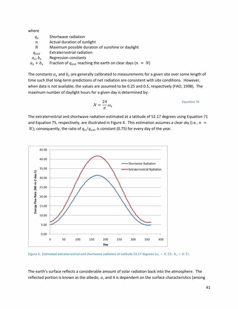
41

where

𝑞𝑠 Shortwave radiation 𝑛 Actual duration of sunlight 𝑁 Maximum possible duration of sunshine or daylight

𝑞𝑒𝑥𝑡 Extraterrestrial radiation 𝑎𝑠, 𝑏𝑠 Regression constants

𝑎𝑠 + 𝑏𝑠 Fraction of 𝑞𝑒𝑥𝑡 reaching the earth on clear days (𝑛 = 𝑁)

The constants 𝑎𝑠 and 𝑏𝑠 are generally calibrated to measurements for a given site over some length of

time such that long-term predictions of net radiation are consistent with site conditions. However,

when data is not available, the values are assumed to be 0.25 and 0.5, respectively (FAO, 1998). The

maximum number of daylight hours for a given day is determined by:

𝑁 =24

𝜋𝜔𝑠

Equation 76

The extraterrestrial and shortwave radiation estimated at a latitude of 52.17 degrees using Equation 71

and Equation 75, respectively, are illustrated in Figure 4. This estimation assumes a clear sky (i.e., 𝑛 =

𝑁); consequently, the ratio of 𝑞𝑠 𝑞𝑒𝑥𝑡⁄ is constant (0.75) for every day of the year.

Figure 4. Estimated extraterrestrial and shortwave radiation at Latitude 52.17 degrees (𝒂𝒔 = 𝟎. 𝟐𝟓; 𝒃𝒔 = 𝟎. 𝟓).

The earth’s surface reflects a considerable amount of solar radiation back into the atmosphere. The

reflected portion is known as the albedo, 𝛼, and it is dependent on the surface characteristics (among

0.00

5.00

10.00

15.00

20.00

25.00

30.00

35.00

40.00

45.00

0 50 100 150 200 250 300 350 400

Ene

rgy

Flu

x R

ate

(M

J m

-2 d

ay-1

)

Day

Shortwave Radiation

Extraterrestrial Radiation

42

other parameters). For example, the albedo of green vegetation is approximately 0.23 while that of

fresh white snow is approximately 0.95 (FAO, 1998). The net solar radiation reaching the earth’s surface

(direct and diffuse), 𝑞𝑛𝑠, also known as the short-wave radiation, is given as:

𝑞𝑛𝑠 = (1 − 𝛼)𝑞𝑠 Equation 77

where the net solar radiation is measured on a horizontal surface. The albedo is often based on field

measurements or is estimated from literature values.

If the net solar radiation is measured directly, albedo can be used as a calibration coefficient. In that

case, albedo incorporates the reflective property of the surface as well as a parameterization for cloud

cover (as above) and angle of incidence/shadowing. The latter is important in hilly terrain in which

some portion of the ground might be obstructed from direct sunlight. Dingman (2008) demonstrates

procedures for incorporating all of these effects. A simple modification to Equation 77 for shadowing

effects results in the expression:

𝑞𝑛𝑠 = (1 − 𝛼)𝑞𝑠 × 𝑉𝐹 Equation 78

where 𝑉𝐹 is a view factor (which varies from 0 to 1) to account for angle of incidence and shadowing.

4.3.1.1.2 Net (Terrestrial) Longwave Radiation

A portion of the net solar radiation incident on the earth’s surface is absorbed and converted into heat

energy. Radiation is emitted from any heated surface due to the thermal energy of the surface matter.

The rate of energy release per unit area of heated surface is the surface emissive power (Incropera et

al., 2007). The upper limit to the emissive power, 𝐸𝑏, is achieved only by a surface called an ideal

radiator (or blackbody), and is described by the Stefan-Boltzmann law:

𝐸𝑏 = 𝜎𝑇𝑔4 Equation 79

where

𝜎 Stefan-Boltzmann constant = 4.903×10-9 MJ/K4/m2/day = 5.67×10-8 W/m2/K4

𝑇𝑔 Absolute temperature of the (ground) surface

The energy emitted by a real surface, known as the long-wave radiation, 𝐸, is less than that of a

blackbody at the same temperature and is given by:

𝐸 = 휀𝑠𝜎𝑇𝑔4 Equation 80

where 휀𝑠 is the surface emissivity and is a value between 0.0 and 1.0. The surface emissivity provides a

measure of how efficiently a surface emits energy relative to a blackbody. Sellers (1965) reports values

of emissivity for dry and moist ground in the range of 0.9 to 0.98. Saito and Simunek (2009) present

various approaches for computing emissivity as a function of water content for bare ground (i.e., no

vegetation). TEMP/W assumes a value of 0.95 for estimating longwave radiation.

43

Some portion of the emitted long-wave radiation is lost into space. A portion is absorbed by water

vapor and CO2 in the atmosphere (including cloud cover). The longwave radiation adsorbed by the

atmosphere increases its temperature and the atmosphere then radiates energy back toward the

ground surface. Consequently, the earth’s surface both emits and receives longwave radiation. The net

longwave radiation is given by (van Bavel and Hillel, 1976):

𝑞𝑛𝑙 = 휀𝑠𝜎𝑇𝑔4 − 휀𝑎휀𝑠𝜎𝑇𝑎

4 Equation 81

where 휀𝑎 and 𝑇𝑎 are the air emissivity and air temperature, respectively. Expressions for air emissivity

vary in the literature. Saito and Simunek (2009) presented air emissivity as a function of near-surface

vapor pressure and/or air temperature. However, Saito and Simunek (2009) noted that most of the

equations performed poorly for their test site. For simplicity, the following expression given by Idso

(1981) is used:

휀𝑎 = 0.70 + 5.95 × 10−5𝑢𝑎𝑒(1500 𝑇𝑎⁄ ) Equation 82

where the atmospheric vapor pressure, 𝑝𝑣𝑎, is calculated using the relationship proposed by Buck (1981)

with an assumed relative humidity of 50%.

4.3.1.1.3 Sensible Heat Flux

Sensible heat flux is a convective heat transfer mechanism that derives its name from the ability to

sense a temperature change caused by energy movement. Sensible heat transport occurs between a

moving fluid (i.e., air) and a bounding surface (i.e., the ground) when the two are at different

temperatures (Incropera et al., 2007). Convective heat transfer involves the combined processes of

conduction (i.e., diffusion of heat through the still boundary layer next to the solid) and heat transfer by

bulk fluid flow, a process referred to as heat advection. Positive sensible heat flux is upward or away

from the surface and occurs when the ground surface is warmer than the air temperature. The rate

equation is of the form:

𝑞𝑠𝑒𝑛𝑠 = ℎ(𝑇𝑔 − 𝑇𝑎) Equation 83

where ℎ is the heat transfer coefficient and the air temperature is usually measured at a reference

height of 2 m (FAO, 1998).

The heat transfer coefficient attempts to accommodate a number of factors, including wind speed and

surface roughness. Expressions for the heat transfer coefficient vary in the literature. Saito and

Simunek (2009) present an equation for sensible heat flux that is in keeping with Dingman (2008). The

equation is:

𝑞𝑠𝑒𝑛𝑠 = 𝐶𝑎

(𝑇𝑔 − 𝑇𝑎)

𝑟𝑎

Equation 84

where 𝑟𝑎 is the aerodynamic resistance to water vapor or heat flow from a soil surface to the

atmosphere, and 𝐶𝑎 is the volumetric heat capacity of air.

44

The aerodynamic resistance can be expressed as:

𝑟𝑎 =1

𝑢𝑘2[𝑙𝑛 (

𝑧𝑟𝑒𝑓 − 𝑑 + 𝑧ℎ

𝑧ℎ) +

ℎ] × [𝑙𝑛 (

𝑧𝑟𝑒𝑓 − 𝑑 + 𝑧𝑚

𝑧𝑚) +

𝑚]

Equation 85

where

𝑢 Wind speed 𝑘 von Karman’s constant = 0.41

𝑧𝑟𝑒𝑓 Reference height for measurements (typically 1.5 m)

𝑑 Zero-plane displacement height 𝑧ℎ,𝑚 Surface roughness height for heat and momentum flux, respectively

ℎ,𝑚 Atmospheric stability correction factor for momentum and heat flux

The zero-plane displacement height, 𝑑, is generally assumed to be 2/3 the vegetation height, while the

surface roughness values, 𝑧ℎ and 𝑧𝑚, are assumed to be 0.1 and 0.123 times the vegetation height,

respectively (Dingman, 2008; Saito and Simunek, 2009). The typical surface roughness height for bare

ground is 0.001 m, with a zero-plane displacement height of zero. It is generally assumed that the

resistance to momentum and heat flow are the same, so the heat and momentum flux surface

roughness values are assumed equivalent (i.e., 𝑧ℎ = 𝑧𝑚).

The atmospheric stability correction factors for momentum and heat flux are assumed equal. In

general, determination of the factors requires an iterative solution. Saito and Simunek (2009) found

that a simplified correction, which was developed by Koivusalo et al. (2001), performed equally as well.

The correction requires the calculation of the Richardson number, 𝑅𝑖, as:

𝑅𝑖 =𝑔 (𝑧𝑟𝑒𝑓)(𝑇𝑎 − 𝑇𝑔)

(𝑇𝑎)𝑢2

Equation 86

The stability correction for stable and unstable conditions is:

= (1 − 10𝑅𝑖)−1 for Ri < 0 = (1 + 10𝑅𝑖)−1 for Ri > 0

Equation 87

The aerodynamic resistance is calculated by setting = 0 in Equation 85, which yields the neutral

aerodynamic resistance, 𝑟𝑎𝑎. The aerodynamic resistance is then calculated using the non-zero value of

the stability correction from Equation 87:

𝑟𝑎 = 𝑟𝑎𝑎 Equation 88

4.3.1.1.4 Latent heat flux

Latent heat refers to the amount of energy released or absorbed by water during a change of state that

occurs without changing its temperature. The term latent infers that energy is being stored in the water

molecules and can be released during condensation. The latent heat of vaporization of water is 2.45

MJ/kg at 20 °C; thus, it takes 2.45 MJ of energy to evaporate 1 kg of water, which is equivalent to 1 mm

45

of water over a square meter of area given a water density of 1000 kg/m3. The latent heat flux in

Equation 69 is given by:

𝑞𝑙𝑎𝑡 = 𝐴𝐸 (1

1000) 𝜌𝑤ℎ𝑠𝑓

Equation 89

where 𝐴𝐸 is the actual evapotranspiration. The actual evaporation can be established using two options

in TEMP/W: 1) user-defined; and, 2) ‘From Water Transfer Analysis’. The first option requires the

definition of an AE verses time function using measured or estimated data. The second option requires

a SEEP/W analysis with a land-climate interaction boundary condition.

4.3.1.1.5 Accommodating the Snowpack

The surface energy balance equation can be re-written to accommodate the presence of snow during

the winter months as:

𝑞𝑠𝑛𝑜𝑤 = 𝑞𝑔 = (𝑞𝑛𝑠 − 𝑞𝑛𝑙) − 𝑞𝑠𝑒𝑛𝑠 − 𝑞𝑙𝑎𝑡 Equation 90

where the energy flux through the snow, 𝑞𝑠𝑛𝑜𝑤, is assumed equal to the ground heat flux. This

assumption requires that the snow has no capacity to store energy. For implementation purposes,

Equation 90 is recast as:

0 = −(𝑞𝑛𝑠 − 𝑞𝑛𝑙) + 𝑞𝑠𝑒𝑛𝑠 + 𝑞𝑙𝑎𝑡 + 𝑞𝑠𝑛𝑜𝑤 Equation 91

The sensible heat flux (Equation 84) and net longwave radiation (Equation 81) are calculated using the

temperature at the top of the snow (not the ground temperature). The energy flux through the snow is

given by:

𝑞𝑠𝑛𝑜𝑤 = −𝑘𝑠𝑛𝑜𝑤

(𝑇𝑔 − 𝑇𝑠𝑛𝑜𝑤)

ℎ𝑠𝑛𝑜𝑤

Equation 92

where

𝑘𝑠𝑛𝑜𝑤 Thermal conductivity of snow 𝑇𝑠𝑛𝑜𝑤 Temperature at snow surface

𝑇𝑔 Temperature at ground surface

ℎ𝑠𝑛𝑜𝑤 Depth of snow

The implicit assumption of this approach is that the specific heat capacity (i.e., the ability to store or

release energy) of the snow pack is negligible relative to the energy flux through the snow. A downward

heat flux through the snow is considered positive as this implies warming of the ground. Latent heat

flux is assumed to be zero during the winter.

4.3.1.2 Inputs

Table 12 summarizes the most rigorous inputs for the SEB boundary condition associated with each of

the energy flux components. The net radiation energy flux drives the other processes and is naturally a

principal input for the SEB boundary condition. In order to calculate sensible heat flux, both the air

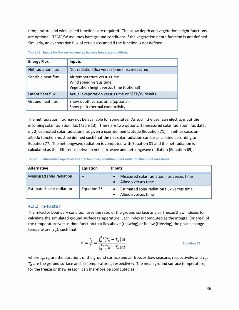
46

temperature and wind speed functions are required. The snow depth and vegetation height functions

are optional. TEMP/W assumes bare ground conditions if the vegetation depth function is not defined.

Similarly, an evaporative flux of zero is assumed if the function is not defined.

Table 12. Inputs for the surface energy balance boundary condition.

Energy Flux Inputs

Net radiation flux Net radiation flux versus time (i.e., measured)

Sensible heat flux Air temperature versus time Wind speed versus time Vegetation height versus time (optional)

Latent heat flux Actual evaporation versus time or SEEP/W results

Ground heat flux Snow depth versus time (optional) Snow pack thermal conductivity

The net radiation flux may not be available for some sites. As such, the user can elect to input the

incoming solar radiation flux (Table 13). There are two options: 1) measured solar radiation flux data;

or, 2) estimated solar radiation flux given a user-defined latitude (Equation 71). In either case, an

albedo function must be defined such that the net solar radiation can be calculated according to

Equation 77. The net longwave radiation is computed with Equation 81 and the net radiation is

calculated as the difference between net shortwave and net longwave radiation (Equation 69).

Table 13. Alternative inputs for the SEB boundary condition if net radiation flux is not measured.

Alternative Equation Inputs

Measured solar radiation -- Measured solar radiation flux versus time

Albedo versus time

Estimated solar radiation Equation 75 Estimated solar radiation flux versus time

Albedo versus time

4.3.2 n-Factor

The n-Factor boundary condition uses the ratio of the ground surface and air freeze/thaw indexes to

calculate the simulated ground surface temperature. Each index is computed as the integral (or area) of

the temperature versus time function that lies above (thawing) or below (freezing) the phase change

temperature (𝑇0), such that

𝑛 =𝐼𝑔

𝐼𝑎=

∫ (𝑇0 − 𝑇𝑔)d𝑡𝑡𝑔

0

∫ (𝑇0 − 𝑇𝑎)d𝑡𝑡𝑎

0

Equation 93

where 𝑡𝑔, 𝑡𝑎 are the durations of the ground surface and air freeze/thaw seasons, respectively; and 𝑇𝑔,

𝑇𝑎 are the ground surface and air temperatures, respectively. The mean ground surface temperature,

for the freeze or thaw season, can therefore be computed as

47

𝑇𝑔 = 𝑛(𝑇𝑎

− 𝑇0)𝑡𝑎

𝑡𝑠+ 𝑇0 Equation 94

where 𝑇𝑎 is the mean air temperature for the corresponding season. The ground surface temperature at

an instant in time can be computed from the air temperature by simplifying the equation as follows:

𝑇𝑔 = 𝑛(𝑇𝑎 − 𝑇0) + 𝑇0 Equation 95

4.3.2.1 Inputs

The inputs for the n-Factor boundary condition are:

Air temperature as a function of time

n-Factor for thawing conditions

n-Factor for freezing conditions

The magnitude of freezing and thawing n-Factors depends on the climatic conditions, as well as on the

material type at the ground surface.

4.3.3 Convective Surface and Thermosyphon

The Convective Surface and Thermosyphon boundary conditions both apply Newton’s Law of Cooling to

calculate a heat flux. The heat flux is then: a) numerically integrated over a surface area to apportion an

energy flux rate to the nodes associated with the surface (second-type); or b) multiplied by a user

entered convective surface area (e.g., perimeter of pipe x 1 unit length into page) to obtain an energy

rate applied to a single node.

4.3.3.1 Newton’s Law of Cooling

Convective heat transport is assumed to occur between a moving fluid and a bounding surface when the

two are at different temperatures (Incropera et. al, 2007). Convective heat transfer involves the

combined processes of conduction (i.e., diffusion of heat through the still boundary layer next to the

solid surface) and heat transfer by bulk fluid flow, referred to as heat advection. The rate equation

describing convective heat transfer (Newton’s Law of Cooling) is:

𝑞𝑠𝑢𝑟 = ℎ(𝑇𝑠𝑢𝑟 − 𝑇∞) Equation 96

where 𝑞𝑠𝑢𝑟 is the surface heat flux due to convection, ℎ is the convection heat transfer coefficient, 𝑇𝑠𝑢𝑟

temperature of the bounding surface, and 𝑇∞ the temperature of the fluid outside the thermal

boundary layer. The thermal boundary layer develops in response to the velocity boundary layer – the

zone in which there are high velocity gradients. A positive heat flux indicates energy transfer from a

warm surface to a cooler fluid.

4.3.3.2 Inputs: Convective Surface

The inputs for the convective surface boundary condition are:

Fluid temperature as a function of time

Convective heat transfer coefficient, ℎ, versus time

Convective surface area (only if the boundary condition is applied to a point)

48

A convective surface boundary condition can be used to simulate artificial ground freezing or other

processes that involve fluid flow over a surface. For example, Andersland and Ladanyi (2004) explore

the use of a convective surface boundary condition to represent the surface energy balance at the

ground surface. For cases involving internal flow through a conduit, heat transfer occurs by conduction

through the conduit wall and then by convective heat transfer from the inside wall of the conduit into

the flowing fluid. In a numerical analysis, however, the convection heat transfer coefficient embodies

the conditions within the boundary layer, as well as the heat transfer characteristics and geometry of

the conduit. Thus, the boundary condition is applied at the outside conduit wall.

The area of the convective surface is calculated via numerical integration if the boundary condition is

applied to an edge comprised of line segments. In contrast, application of the boundary condition to a

point, which inherently has no area, requires specification of the surface perimeter. The surface

perimeter, which is equal to the outside circumference of a pipe in ground freezing applications, is

multiplied by the element thickness to obtain the surface area.

Incropera et al. (2007) describes the difficulties in defining the convection coefficient a priori. In

addition to depending on numerous fluid properties such as density, viscosity, thermal conductivity, and

specific heat capacity, the convection coefficient depends on the surface geometry and flow conditions.

The convection coefficient can be obtained by solving the boundary layer equations for simple flow

situations. The more practical approach involves calculation of a Nusselt number, Nu, and subsequent

calculation of a convection heat transfer coefficient from the functional relationship:

Nu =ℎ𝐿

𝑘𝑓

Equation 97

where 𝑘𝑓 is the thermal conductivity of the fluid and 𝐿 is a characteristic length (e.g., hydraulic diameter

= outer diameter – inner diameter). The Nusselt number can vary with time in response to the flow

conditions (i.e., laminar or turbulent), temperature gradients, and other factors; consequently, the

convection heat transfer coefficient is input as a function of time. The convection heat transfer

coefficient for brine freezing applications typically ranges between 25 and 75 W/m2/°C.

4.3.3.3 Inputs: Thermosyphon

The inputs for the thermosyphon boundary condition are:

Air temperature as a function of time

Wind speed with time

Convective heat transfer coefficient versus wind speed

Surface perimeter (only if the boundary condition is applied to a point)

Maximum operating air temperature

Minimum temperature difference for vaporization

A common application of a thermosyphon is to maintain frozen conditions beneath surface

infrastructure, such as a roadway, constructed over permafrost. Thermosyphons transfer heat from the

49

ground if the air temperature moving past the condenser is less than ground temperature.

Thermosyphons comprise an evaporator section installed in the ground and a condenser section

exposed to atmospheric conditions.

The overall heat conductance of a thermosyphon is defined as the heat rate extracted from the device

divided by the temperature difference between the evaporator and air flowing past the condenser.

Haynes and Zarling (1988), for example, measured overall heat conductance of a thermosyphon by

placing the condenser in a wind tunnel maintained at constant temperature. The evaporator was also

maintained at a constant temperature via a heated water bath. The overall heat conductance was

measured at various wind speeds and the data described by empirical relationships of the form:

𝐻𝑒𝑎𝑡 𝑡𝑟𝑎𝑛𝑠𝑓𝑒𝑟 𝑐𝑜𝑛𝑑𝑢𝑐𝑡𝑎𝑛𝑐𝑒 = 𝐴 + 𝐵(𝑢𝑛) Equation 98

where 𝐴 and 𝐵 are coefficients, 𝑛 an exponent, and 𝑢 the fluid (wind) velocity. The convection heat

transfer coefficient can be calculated by dividing the overall heat conductance by the total area of the

evaporator, and input as a function of wind speed.

Heat transfer through the thermosyphon ceases if: a) the air temperature is greater than the ground

temperature; b) the air temperature exceeds a user specified maximum operating value; or, c) the

temperature difference between the air and outside wall of the evaporator (i.e., ground) is not great

enough to cause vaporization of the fluid (e.g., C02 or Anhydrous Ammonia).

Thermosyphons are most commonly applied to circular openings (i.e., edges of elements) or to a point

(i.e., node) in a 2D analysis. The evaporator of the thermosyphon is viewed in cross-section when the

boundary condition is applied in this manner. Similar to the convective surface boundary condition, the

surface area of the evaporator section is calculated via numerical integration when the boundary

condition is applied to an edge comprising line segments. In contrast, application of the boundary

condition to a point, which inherently has no area, requires specification of the surface perimeter. The

surface perimeter, which is equal to the outside circumference of the evaporator, is multiplied by the

element thickness to obtain the surface area of the evaporator. The thermosyphon boundary condition

can also be applied to a line in an axisymmetric analysis to model a single vertical thermosyphon.


4.3.4.1 Sinusoidal Distribution of Cumulative Daily Radiation

Cumulative daily net radiation and cumulative daily shortwave radiation are the time-integrated values

of the radiation flux (e.g., Figure 4). The cumulative daily radiation is often reported as an energy flux;

however, it is more appropriate to consider this measurement as the total quantity of energy over a unit

area of the ground surface in one day. The user has the option to apply the cumulative daily radiation

flux directly, which is equivalent to assuming that the flux rate is constant over the day. There is also the

option to distribute sinusoidally over each day. The radiation flux at any instant during the day is then

estimated from the cumulative value as:

(𝑞𝑛𝑠 − 𝑞𝑛𝑙) = 𝐴𝑠𝑖𝑛𝜃 Equation 99

50

where

𝐴 = Normalized Amplitude = (𝜋 2𝑁⁄ )

𝜃 = Normalized time (0 < 𝜃 < 𝜋) Figure 5 presents the incoming solar radiation flux associated with a sinusoidal distribution of

cumulative daily solar radiation. Sunrise and sunset are assumed to occur symmetrically around noon

based on the maximum number of daylight hours for a given day (Equation 76). Net radiation is

generally non-zero before and after sunrise and sunset, respectively, because the ground continues to

emit net longwave radiation. However, the option to distribute a cumulative daily net radiation value

assumes that the net radiation is zero before sunrise and after sunset.

Figure 5. Example of sinusoidal radiation flux.

5 Air Transfer with AIR/W AIR/W is a finite element program for simulating air transfer. Although it can be a standalone product,

the true power in the AIR/W formulation lies with the increased functionality it provides when

combined with other GeoStudio products. For example, AIR/W can be coupled with TEMP/W to model

forced convection heat transfer, with CTRAN/W to model gas transfer via advection, or with SEEP/W to

model coupled air-water systems. Section 5.1 summarizes the air transfer and storage processes

included in the formulation. Section 5.2 describes the constitutive models available to characterize the

air transfer and storage processes of the medium. Section 5.3 describes the boundary conditions that

are unique to this product beyond the basic FEM boundary conditions described in Section I.7.

5.1 Theory The AIR/W formulation is based on the mass conservation statement (Equation 1 in Section 3.1). The

rate of change in the mass of air stored in the REV is given by:

Cumulative Daily Solar Radiation

So

lar

Ra

dia

tio

n F

lux

(M

J/d

ay

s/m

²)

Time (days)

0

10

20

30

40

0 1 2 3 4 5

51

��𝑔 = ��𝑎 + ��𝑑 + ��𝑣 Equation 100

The subscript 𝑔 has been used denote pore-gas, which comprises dry air (𝑎), dissolved dry air (𝑑), and

water vapor (𝑣). The mass of dissolved air and water vapor are assumed negligible and are omitted

from the AIR/W formulation. The rate of change in the mass of dry air within the control volume is

calculated with the ideal gas law (see Equation 5):

��𝑎 =𝜕𝑀𝑎

𝜕𝑡=

𝑀

𝑅[𝜃𝑎

𝑇

𝜕𝑢𝑎

𝜕𝑡+

��𝑎

𝑇

𝜕𝜃𝑎

𝜕𝑡+ ��𝑎𝜃𝑎

𝜕

𝜕𝑡(

1

𝑇)] 𝑑𝑥 𝑑𝑦 𝑑𝑧

Equation 101

where 𝑀 is the molar mass, 𝑅 is the gas constant, 𝜃𝑎 is the volumetric air content, 𝑢𝑎 is pore air

pressure, and ��𝑎 absolute air pressure. The temporal derivative of the volumetric air content is equal to

the negative of the temporal derivative of the volumetric water content:

𝜕𝜃𝑎

𝜕𝑡= −

𝜕𝜃𝑤

𝜕𝑡= − (𝑚𝑤

𝜕𝑢𝑎

𝜕𝑡− 𝑚𝑤

𝜕𝑢𝑤

𝜕𝑡)

Equation 102

where 𝑚𝑤 is the slope of the volumetric water content function.

The air mass flow rate in response to mechanical energy gradients follows a similar form as Darcy’s Law

for variable density liquid water flow:

��𝑎 = 𝜌𝑎𝑞𝑎𝑑𝑥𝑑𝑧 =−𝑘𝑎

𝑔(

𝜕𝑢𝑎

𝜕𝑦+ 𝜌𝑎𝑔

𝜕𝑦

𝜕𝑦) 𝑑𝑥𝑑𝑧

Equation 103

where 𝑞𝑎 is the volumetric air flux and 𝑘𝑎 is the (dry) air hydraulic conductivity. Substitution and

expansion of Equation 101 and Equation 103 into the conservation statement and division by the

volume of the REV gives:

𝜌𝑎

[(𝜃𝑎

��𝑎

− 𝑚𝑤)𝜕𝑢𝑎

𝜕𝑡+ 𝑚𝑤

𝜕𝑢𝑤

𝜕𝑡+ 𝑇𝜃𝑎

𝜕

𝜕𝑡(

1

𝑇)] =

𝜕

𝜕𝑦[𝑘𝑎

𝑔(

𝜕𝑢𝑎

𝜕𝑦+ 𝜌

𝑎𝑔

𝜕𝑦

𝜕𝑦)]

Equation 104

Equation 104 can be simplified by assuming isothermal conditions with constant water content (i.e.,

single-phase air transfer):

𝜌𝑎

𝜃𝑎

��𝑎

=𝜕

𝜕𝑦[𝑘𝑎

𝑔(

𝜕𝑢𝑎

𝜕𝑦+ 𝜌

𝑎𝑔

𝜕𝑦

𝜕𝑦)]

Equation 105

Table 14 summarizes the physical processes included in the partial differential equation solved by

AIR/W. The left side of Equation 104 includes the rate of change in the mass of air due to changes in air

density and air content. The formulation implicitly includes the effect of changes in pore-air pressure

52

and temperature on storage via the ideal gas law. Changes in air content are linked to changes in water

content and, therefore, pore-water pressure. The right side of Equation 104 includes air transfer in

response to gradients in pore-air pressure and density.

Table 14. Summary of the physical processes included in the AIR/W formulation.


Storage: air compressibility AIR/W

Storage: soil structure compressibility AIR/W + SEEP/W

Storage: matric suction changes due to pore-water pressure changes AIR/W + SEEP/W

Storage: matric suction changes due to pore-air pressure changes AIR/W + SEEP/W

Storage: air density changes due to temperature changes AIR/W + TEMP/W

Flow: pressure-driven (isothermal) AIR/W

Flow: gravity-driven AIR/W

Flow: density-driven via thermal effects (free convection) AIR/W + TEMP/W

The key elements of the AIR/W formulation are as follows:

The default physical processes in AIR/W include pressure and gravity-driven flow and storage

changes due to changes in air pressure.

Thermal effects on air density, which exerts control on both storage and flow, are included by

coupling AIR/W and TEMP/W. This is achieved by selecting the option for free convection:

thermal effects.

AIR/W can be coupled with SEEP/W to simultaneously model water transfer and its effect on air

transfer and storage (and vice versa). This is achieved by solving air and water transfer on the

same domain. Thermal effects can also be included with this type of analysis (AIR/W + SEEP/W

+ TEMP/W).

5.2 Material Models

5.2.1 Single Phase

Single phase pore-air transfer through porous media can be modelled assuming that the volumetric air

content (and water content) are constant. This material model can be applied to AIR/W and coupled

AIR/W-TEMP/W analyses, but not for coupled AIR/W-SEEP/W analyses. The parameters required for

this material model are presented in Table 15. Air conductivity is assumed to be isotropic for this

material model. Changes in air storage are a function of the air content and air density, with the latter

calculated internally according to the ideal gas law.

Table 15. Parameters for the single-phase material model.

53


Air Conductivity 𝑘𝑎 m/s

Volumetric Air Content 𝜃𝑎 m2/kN

5.2.2 Dual Phase

The dual-phase material model is required for coupled AIR/W-SEEP/W analyses. The parameters

required for this material model are presented in Table 16. Air conductivity governs the resistance to

flow and is entered as a function of saturation. The air content is no longer an input because it is

determined directly from the volumetric water content function used in the SEEP/W water transfer

analysis. As in the single-phase material model, air density is calculated according to the ideal gas law

given the air pressure and temperature.

Table 16. Parameters for the single-phase material model.


Air Conductivity Function 𝑘𝑎(𝑆) m/s


5.2.3.1 Air Conductivity Function

GeoStudio uses the closed-form equation presented by Fredlund and Xing (1994) to estimate the air

conductivity function. The equation is given as:

𝑘𝑎 = 𝑘𝑑𝑟𝑦(1 − 𝑆)1

2⁄ (1 − 𝑆1

𝑞⁄ )2𝑞

Equation 106

where 𝑘𝑑𝑟𝑦 is the air conductivity of the dry soil, 𝑆 is the saturation of the soil, and 𝑞 is a curve fitting

parameter related to pore-size distribution (assumed to be 2.9 after Fredlund et al., 2012).

5.3 Boundary Conditions The conventional first and second type boundary conditions as described in Section 0 can be used within

an air flow analysis. However, simulating the effect of atmospheric air pressure on the ground surface

requires a unique boundary condition.

5.3.1 Barometric Air Pressure

The barometric air pressure boundary condition is used to simulate the variability in atmospheric air

pressure along a sloping ground surface. The air pressure, 𝑢𝑎𝑦, at an arbitrary elevation, 𝑦, is calculated

according to the barometric formula:

𝑢𝑎𝑦= ��𝑎0

𝑒(

−𝑀𝑔𝑅𝑇𝑎

(𝑦−𝑦0))− ��𝑎𝑁𝐼𝑆𝑇

Equation 107

54

where ��𝑎0 is the atmospheric air pressure measured at the elevation 𝑦0 and air temperature 𝑇𝑎, and

��𝑎𝑁𝐼𝑆𝑇 the standard atmospheric pressure at sea level (i.e. 101.325 kPa). Absolute pressure is zero-

referenced against a perfect vacuum while gauge pressure is zero-referenced against the ambient air

pressure. Absolute pressure is therefore equal to atmospheric pressure plus gauge pressure. Exposure

of an absolute pressure measurement device to the atmosphere allows for measurement of barometric

air pressure, which naturally corresponds to a gauge pressure of zero. The air pressure 𝑢𝑎𝑦 in Equation

107 must therefore be thought of as a differential pressure; that is, the air pressure measured by a

device that is zero referenced against standard atmospheric pressure at sea level.

55

6 Solute and Gas Transfer with CTRAN/W CTRAN/W is a finite element program for simulating the transport of a dissolved constituent or gas

through porous media. Typical applications for CTRAN/W include dissolved solute or gas transport

through regional or local groundwater flow systems, or oxygen transport through air and water within

unsaturated mine waste. Section 6.1 summarizes the solute and gas transfer and storage processes

included in the CTRAN/W formulation. Section 6.2 describes the constitutive models available to

characterize the solute and gas transfer and storage processes, and Section 6.3 describes the boundary

conditions unique to this product.

6.1 Theory The governing equations for solute and gas transfer in CTRAN/W are based on the law of mass

conservation in the same manner as the water (Section 3.1) and air (Section 5.1) transfer formulations.

6.1.1 Solute Transfer

The rate of change in the mass of solute stored in a control volume is given by:

��𝑠𝑡 = ��𝑑𝑝 + ��𝑎𝑝 Equation 108

The subscript 𝑑𝑝 and 𝑎𝑝 have been used to denote dissolved and adsorbed phases. This equation can be expanded to:

��𝑠𝑡 =𝜕

𝜕𝑡(𝐶𝜃𝑤 + 𝜌𝑑

𝜕𝑆∗

𝜕𝑡) 𝑑𝑥 𝑑𝑦 𝑑𝑧

Equation 109

where 𝐶 is the mass concentration in the dissolved phase, 𝜌𝑑 is the dry bulk density of the soil (𝑀𝑠 𝑉𝑡⁄ ),

and 𝑆∗ is the quantity of mass (𝑀) sorbed per mass of solids (𝑀𝑠).

First order kinematic reactions such as radioactive decay, biodegradation, and hydrolysis result in mass

consumption within the control volume. Thus, a sink term is now included in the conservation

statement (��𝑆) to represent the first order reaction processes. The rate of change in the solute mass

due to decay, ��𝜆, is given by:

��𝜆 = −𝜆(𝜃𝑤𝐶 + 𝜌𝑑𝑆∗) 𝑑𝑥 𝑑𝑦 𝑑𝑧 = −��𝑆 Equation 110

where 𝜆 is the reaction constant.

The mass flow rate in response to concentration gradients, ��𝐷, can be evaluated according to Fick’s

Law:

��𝑫 = 𝑱𝑫𝒅𝒙𝒅𝒛 = −𝑫𝒅∗ 𝜽𝒘

𝝏𝑪

𝝏𝒚𝒅𝒙𝒅𝒛

Equation 111

56

where 𝐽𝐷 is the diffusion mass flux and 𝐷𝑑∗ is the bulk diffusion coefficient, which accounts for the effects

of tortuosity. The bulk diffusion coefficient can be replaced by a coefficient of hydrodynamic dispersion

that incorporates the combined effects of diffusion and mechanical dispersion:

𝐷 = 𝐷′ + 𝐷𝑑∗ Equation 112

where 𝐷′ is the coefficient of mechanical dispersion, which can be expanded to give:

𝐷 = 𝛼𝑣𝑤 + 𝐷𝑑∗ Equation 113

where 𝛼 is the dispersivity of the medium and 𝑣𝑤 is the groundwater velocity. It is important to note

that mechanical dispersion is represented as a tensor rather than a scalar in multi-dimensional problems

while the bulk diffusion coefficient is represented as a scalar.

Advection solute transport is mass transport due to the flow of water in which the mass is dissolved.

The direction and rate of transport coincide with the groundwater flow. The groundwater flux is

described by the Darcy Equation. The advective mass flow rate, ��𝐴, is given by:

��𝐴 = 𝐽𝐴𝑑𝑥𝑑𝑧 = (𝜃𝑤𝐶)𝑣𝑤𝑑𝑥𝑑𝑧 = 𝐶𝑞𝑤𝑑𝑥𝑑𝑧 Equation 114

where 𝐽𝐴 is the advective mass flux, (𝜃𝑤𝐶) is the amount of dissolved mass relative to the control

volume, and 𝑞𝑤 is the water flux, which is related to the linear groundwater velocity by 𝑞𝑤/𝜃𝑤.

Substitution and expansion of the foregoing rate equations into the conservation statement and division

by the dimensions of the control volume gives:

(𝜃𝑤 + 𝜌𝑑

𝜕𝑆∗

𝜕𝐶)

𝜕𝐶

𝜕𝑡+ 𝐶

𝜕𝜃𝑤

𝜕𝑡=

𝜕

𝜕𝑦[𝐷𝜃𝑤

𝜕𝐶

𝜕𝑦− 𝐶𝑞𝑤] − 𝜆(𝜃𝑤𝐶 + 𝜌𝑑𝑆)

Equation 115

where 𝜕𝑆∗/𝜕𝐶 is the equilibrium sorption isotherm or the adsorption coefficient (𝐾𝑑).


CTRAN/W for solute transfer. The left side of Equation 115 includes rates of mass change in response to

concentration changes, adsorption, and water content changes. The right side of Equation 115 includes

solute transfer via diffusion and advection-dispersion, along with the first order reaction losses from the

dissolved and adsorbed mass.

Table 17. Summary of the physical processes included in the CTRAN/W solute transfer formulation.


Storage: concentration changes CTRAN/W + SEEP/W

Storage: water content changes CTRAN/W + SEEP/W

Storage: adsorption CTRAN/W + SEEP/W

Storage: decay of dissolved and adsorbed mass CTRAN/W + SEEP/W

Flow: diffusion CTRAN/W + SEEP/W

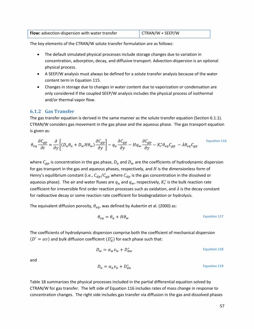
57

Flow: advection-dispersion with water transfer CTRAN/W + SEEP/W

The key elements of the CTRAN/W solute transfer formulation are as follows:

The default simulated physical processes include storage changes due to variation in

concentration, adsorption, decay, and diffusive transport. Advection-dispersion is an optional

physical process.

A SEEP/W analysis must always be defined for a solute transfer analysis because of the water

content term in Equation 115.

Changes in storage due to changes in water content due to vaporization or condensation are

only considered if the coupled SEEP/W analysis includes the physical process of isothermal

and/or thermal vapor flow.

6.1.2 Gas Transfer

The gas transfer equation is derived in the same manner as the solute transfer equation (Section 6.1.1).

CTRAN/W considers gas movement in the gas phase and the aqueous phase. The gas transport equation

is given as:

𝜃𝑒𝑞

𝜕𝐶𝑔𝑝

𝜕𝑡=

𝜕

𝜕𝑦[(𝐷𝑎𝜃𝑎 + 𝐷𝑤𝐻𝜃𝑤)

𝜕𝐶𝑔𝑝

𝜕𝑦] − 𝑞𝑎

𝜕𝐶𝑔𝑝

𝜕𝑦− 𝐻𝑞𝑤

𝜕𝐶𝑔𝑝

𝜕𝑦− 𝐾𝑟

∗𝜃𝑒𝑞𝐶𝑔𝑝 − 𝜆𝜃𝑒𝑞𝐶𝑔𝑝 Equation 116

where 𝐶𝑔𝑝 is concentration in the gas phase, 𝐷𝑎 and 𝐷𝑤 are the coefficients of hydrodynamic dispersion

for gas transport in the gas and aqueous phases, respectively, and 𝐻 is the dimensionless form of

Henry’s equilibrium constant (i.e., 𝐶𝑑𝑝/𝐶𝑔𝑝 where 𝐶𝑑𝑝 is the gas concentration in the dissolved or

aqueous phase). The air and water fluxes are 𝑞𝑎 and 𝑞𝑤, respectively, 𝐾𝑟∗ is the bulk reaction rate

coefficient for irreversible first order reaction processes such as oxidation, and 𝜆 is the decay constant

for radioactive decay or some reaction rate coefficient for biodegradation or hydrolysis.

The equivalent diffusion porosity, 𝜃𝑒𝑞, was defined by Aubertin et al. (2000) as:

𝜃𝑒𝑞 = 𝜃𝑎 + 𝐻𝜃𝑤 Equation 117

The coefficients of hydrodynamic dispersion comprise both the coefficient of mechanical dispersion

(𝐷′ = 𝛼𝑣) and bulk diffusion coefficient (𝐷𝑑∗) for each phase such that:

𝐷𝑤 = 𝛼𝑤𝑣𝑤 + 𝐷𝑑𝑤∗ Equation 118

and

𝐷𝑎 = 𝛼𝑎𝑣𝑎 + 𝐷𝑑𝑎∗ Equation 119


CTRAN/W for gas transfer. The left side of Equation 116 includes rates of mass change in response to

concentration changes. The right side includes gas transfer via diffusion in the gas and dissolved phases

58

and advection-dispersion in the gas and dissolved phases. The formulation also includes the decay of

mass within the gaseous and aqueous phases, as well as first order reaction processes (i.e.,

consumption).

Table 18. Summary of the physical processes included in the CTRAN/W gas transfer formulation.


Storage: concentration changes CTRAN/W + SEEP/W

Storage: decay of gas in free and dissolved phases CTRAN/W + SEEP/W

Storage: consumption in the free and dissolved phases CTRAN/W + SEEP/W

Flow: diffusion in the free and dissolved phases CTRAN/W + SEEP/W

Flow: advection-dispersion with water transfer CTRAN/W + SEEP/W

Flow: advection-dispersion with air transfer CTRAN/W + SEEP/W + AIR/W

The key elements of the CTRAN/W gas transfer formulation are as follows:

The default simulated physical processes include concentration changes via decay or reaction

processes, and diffusive transport. Advection-dispersion with water and/or air transfer is an

optional physical process.

A SEEP/W analysis must always be defined for a gas transfer analysis because of the equivalent

diffusion porosity term in Equation 116.

The concentration in the gas and dissolved phases is assumed to be in equilibrium.

6.2 Material Models

6.2.1 Solute Transfer

There is only one material model available in a CTRAN/W analysis. The parameters required for this

material model are presented in Table 19. The bulk diffusion coefficient is defined as a function of water

content and the adsorption is defined as a function of concentration. The first order reaction coefficient

is calculated internally from the specified reaction half-life (Equation 115). The longitudinal and

transverse dispersivity inputs are only visible if advection-dispersion is included in the analysis.

Table 19. Parameters for a solute transfer material model.


Bulk Diffusion Coefficient function 𝐷(𝜃𝑤) m2/s

Adsorption function 𝐾𝑑(𝐶) Mg/Mg

Decay Half-Life 𝑡12⁄ s

Dry Density 𝜌𝑑 Mg/m3

Longitudinal Dispersivity 𝛼𝐿 m

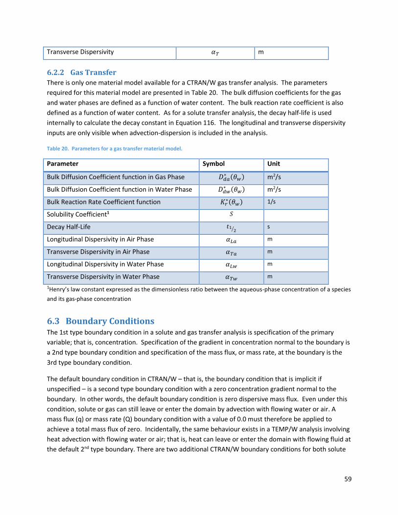
59

Transverse Dispersivity 𝛼𝑇 m

6.2.2 Gas Transfer

There is only one material model available for a CTRAN/W gas transfer analysis. The parameters

required for this material model are presented in Table 20. The bulk diffusion coefficients for the gas

and water phases are defined as a function of water content. The bulk reaction rate coefficient is also

defined as a function of water content. As for a solute transfer analysis, the decay half-life is used

internally to calculate the decay constant in Equation 116. The longitudinal and transverse dispersivity

inputs are only visible when advection-dispersion is included in the analysis.

Table 20. Parameters for a gas transfer material model.


Bulk Diffusion Coefficient function in Gas Phase 𝐷𝑑𝑎∗ (𝜃𝑤) m2/s

Bulk Diffusion Coefficient function in Water Phase 𝐷𝑑𝑤∗ (𝜃𝑤) m2/s

Bulk Reaction Rate Coefficient function 𝐾𝑟∗(𝜃𝑤) 1/s

Solubility Coefficient1 𝑆

Decay Half-Life 𝑡12⁄ s

Longitudinal Dispersivity in Air Phase 𝛼𝐿𝑎 m

Transverse Dispersivity in Air Phase 𝛼𝑇𝑎 m

Longitudinal Dispersivity in Water Phase 𝛼𝐿𝑤 m

Transverse Dispersivity in Water Phase 𝛼𝑇𝑤 m

1Henry’s law constant expressed as the dimensionless ratio between the aqueous-phase concentration of a species

and its gas-phase concentration

6.3 Boundary Conditions The 1st type boundary condition in a solute and gas transfer analysis is specification of the primary

variable; that is, concentration. Specification of the gradient in concentration normal to the boundary is

a 2nd type boundary condition and specification of the mass flux, or mass rate, at the boundary is the

3rd type boundary condition.

The default boundary condition in CTRAN/W – that is, the boundary condition that is implicit if

unspecified – is a second type boundary condition with a zero concentration gradient normal to the

boundary. In other words, the default boundary condition is zero dispersive mass flux. Even under this

condition, solute or gas can still leave or enter the domain by advection with flowing water or air. A

mass flux (q) or mass rate (Q) boundary condition with a value of 0.0 must therefore be applied to

achieve a total mass flux of zero. Incidentally, the same behaviour exists in a TEMP/W analysis involving

heat advection with flowing water or air; that is, heat can leave or enter the domain with flowing fluid at

the default 2nd type boundary. There are two additional CTRAN/W boundary conditions for both solute

60

and gas transfer analyses that require further consideration: (1) source concentration; and (2) free exit

mass flux.

6.3.1 Source Concentration

The source concentration is a special form of the 3rd type boundary in which the mass flux entering the

domain is calculated as the water flux multiplied by the input source concentration.

𝐽𝑠 = 𝐶𝑞𝑛 Equation 120

This boundary condition is useful because the concentration of the pore-fluid at the edge of the

boundary is not necessarily equal to the source concentration at the onset of an analysis due to mass

flux produced by concentration gradients. It is like a mass flux (q) or mass rate (Q) boundary in that the

boundary condition controls the mass flux into the domain; however, in this case the user is specifying

the concentration of the fluid ‘external’ to the domain and allowing the software to calculate mass flux

with the fluid flowing across the domain boundary.

6.3.2 Free Exit Mass Flux

Frind (1988) formulated a modified 3rd type boundary condition to create a free exit boundary condition

for mass flux when the mass flux across the boundary is dependent on the transport processes occurring

inside the domain. This boundary condition allows mass to exit by both advection and dispersion (i.e.,

Cauchy boundary condition) in accordance with the solute concentration arriving at the boundary. The

total surface mass flux at the boundary, 𝐽𝑠, is given by:

𝐽𝑠 = −𝐷𝜃𝑤

𝜕𝐶

𝜕𝑛+ 𝐶𝑞𝑛

Equation 121

where the fluid (air or water) flux, 𝑞𝑛, and concentration gradient are calculated normal to the surface.

The free exit mass flux boundary condition does not require any inputs because the concentration at the

boundary is computed by the solver. The free exit boundary reverts to a zero total mass flux boundary

condition if fluid is entering the domain, which causes a flushing effect given that the fluid is implicitly at

zero concentration.

6.4 Convergence

6.4.1 Dimensionless Numbers

The Péclet and Courant dimensionless numbers can be used to minimize the numerical dispersion and

oscillation that is inherent in the finite element solution of the advection-dispersion equation. The

Péclet number is defined as the ratio of the rate of advection to the rate of diffusion, and thus provides

a measure of the degree to which advection dominates the contaminant transport process. The Courant

number, on the other hand, reflects the portion of an element that is traversed by a solute in one time

step. In one dimensional form, these numbers read as follows

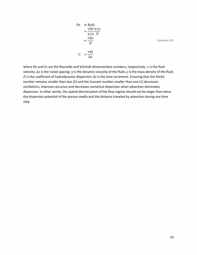
61

Pe ≡ ReSc

=𝑣∆𝑥

𝜂 𝜌⁄

𝜂 𝜌⁄

𝐷

=𝑣∆𝑥

𝐷

Equation 122

C =𝑣∆𝑡

∆𝑥

where Re and Sc are the Reynolds and Schmidt dimensionless numbers, respectively; 𝑣 is the fluid

velocity; ∆𝑥 is the nodal spacing; 𝜂 is the dynamic viscosity of the fluid; 𝜌 is the mass density of the fluid;

𝐷 is the coefficient of hydrodynamic dispersion; ∆𝑡 is the time increment. Ensuring that the Péclet

number remains smaller than two (2) and the Courant number smaller than one (1) decreases

oscillations, improves accuracy and decreases numerical dispersion when advection dominates

dispersion. In other words, the spatial discretization of the flow regime should not be larger than twice

the dispersion potential of the porous media and the distance traveled by advection during one time

step.

62

7 References Allen, R.G., Pereira, Luis S., Raes, D. and Smith, M. 1998. Crop evapotranspiration - Guidelines for

computing crop water requirements - FAO Irrigation and drainage paper 56. Food and Agriculture

Organization of the United Nations.

Andersland, O.B. and Ladanyi, B. 2004. Frozen Ground Engineering, 2nd Edition. John Wiley and Sons

Inc., New Jersey.

Aubertin, M., Aachib, M. and Authier, K. 2000. Evaluation of diffusive gas flux through covers with a

GCL. Geotextiles and Geomembranes, 18: 1-19.

Aubertin, M., Mbonimpa, M., Bussière, B. and Chapuis, R.P. 2003. A model to predict the water

retention curve from basic geotechnical properties. Canadian Geotechnical Journal, 40(6): 1104-1122.

Barbour, S.L. and Fredlund, D.G. 1989. Mechanisms of osmotic flow and volume change in clay soils.

Canadian Geotechnical Journal, 26: 551-552.

Barbour, S.L. and Krahn, J. 2004. Numerical modelling: Prediction or process? Geotechnical News,

December: 44-52.

Bathe, K.J. 2006. Finite Element Procedures. Prentice Hall, Pearson Education Inc.

Ba-Te, B., Zhang, L. and Fredlund, D.G. 2005. A general air-phase permeability function for air flow

through unsaturated soils. Geotechnical Special Publication no. 130 – 142, Geo-Frontiers 2005: 2961-

2985.

Bear, J. 1988. Dynamics of Fluids in Porous Media. American Elsevier Publishing Company, Inc., New

York.

Bear, J. 1979. Hydraulics of Groundwater. McGraw-Hill, New York.

Bowles, J.E. 1988. Foundation analysis and design. Fourth Edition. McGraw-Hill, Inc.

Brutsaert, W. 1975. The roughness length for water vapor, sensible heat and other scalars, Journal of

Atmospheric Sciences. 32: 2028-2031.

Buck, A. L. 1981. New equations for computing vapor pressure and enhancement factor. Journal of

Applied Meteorology, 20: 1527-1532.

Burland, J.B. 1987. Nash Lecture: The Teaching of Soil Mechanics – a Personal View. Proceedings of the

9th ECSMFE, Dublin, vol. 3, pp. 1427-1447.

Burland J.B. 1996. Closing Session Discussions. In: Proceedings of the First International Conference on

Unsaturated Soils, Paris, 6-8 September 1995. Edited by E.E. Alonso and P. Delage. A.A. Balkema. vol. 3,

pp. 1562-1564.

63

Carslaw, H.S. and Jaeger, J.C. 1986. Conduction of Heat in Solids, Oxford Science Publication, 2nd Edition.

Côté, J. and Konrad, J.-M. 2005. A numerical approach to evaluate the risk of differential surface icing

on pavements with insulated surfaces. Cold Regions Science and Technology, 43: 187-206.

Desai, C.S. 1979. Elementary Finite Element Method. Prentice-Hall Inc., Englewood Cliffs, N.J.

de Vries, D.A. 1963. Thermal Properties of Soils. In The Physics of Plant Environment. Edited by W.R.

van Wijk. Amsterdam, p. 382.

de Vries, D.A. 1975. Heat Transfer in Soils. In Heat and Mass Transfer in the Biosphere, 1. Transfer

Process in Plant Environment. Washington, DC, pp. 5-28.

Dingman, S.L. 2008. Physical Hydrology, 2nd Edition. Waveland Press Inc., Long Grove, Illinois.

Domenico, P.A. and Schwartz, W. 1998. Physical and Chemical Hydrogeology. 2nd Edition. John Wiley &

Sons Inc., New York.

Farouki, O.T. 1981. Thermal Properties of Soils. CRREL Monograph 81-1. U.S. Army Corps of Engineers,

Cold Regions Research and Engineering Laboratory, Hanover, New Hampshire.

Food and Agriculture Organization of the United Nations, 1998. Crop Evapotranspiration: Guidelines for

computing crop water requirements.

Fayer, M.J. 2000. UNSAT-H version 3.0: Unsaturated soil water and heat flow model, theory, user

manual, and examples, Rep. 13249, Pacific Northwest National Laboratory, Richland, Washington.

Feddes, R.A., Hoff, H., Bruen, M., Dawson, T. de Rosnay, P., Dirmeyer, P., Jackson, R.B., Kabat, P.,

Kleidon, A., Lilly, A. and Pitman, A.J. 2001. Modeling root water uptake in hydrological and climate

models. Bulletin of the Americal Meteorological Society, 82(12): 2797 – 2809.

Flerchinger, G.N., Kustas, W.P. and Weltz, M.A. 1998. Simulating surface energy fluxes and radiometric

surface temperatures for two arid vegetation communities using the SHAW model. Journal of Applied

Meteorology, 37: 449-60.

Flerchinger, G.N. 2000. The Simultaneous Heat and Water Model: Technical Documentation.

Flerchinger, G.N., Seyfried, M.S. and Hardegree, S.P. 2006. Using soil freezing characteristics to model

multi-season soil water dynamics. Vadose Zone Journal, 5: 1143-1153.

Fredlund, D.G. and Rahardjo, H. 1993. Soil Mechanics for Unsaturated Soils. John Wiley & Sons, Inc. NJ.

Fredlund, D.G., Rahardjo, H. and Fredlund, M.D. 2012. Unsaturated Soil Mechanics in Engineering

Practice. John Wiley & Sons, Inc. NJ.

Fredlund, D.G. and Xing, A. 1994. Equations for the soil-water characteristic curve. Canadian

Geotechnical Journal, 31, 521-532.

64

Freeze, R.A. and Cherry, J.A. 1979. Ground Water. Englewood Cliffs, NJ: Prentice Hall.

Frind, E.O. 1988. Solution of the advection-dispersion equation with free exit boundary. Numerical

Methods for Partial Differential Equations, 4: 301-313.

Hansson, K., Simunek, J., Mizoguchi , M., Lundin, L.-C. and van Genuchten, M.Th. 2004. Water flow and

heat transport in frozen soil: Numerical solution and freeze-thaw applications. Vadose Zone Journal, 3:

693-704.

Harlan, R.L. and Nixon, J.F. 1978. Ground Thermal Regime. Geotechnical Engineering for Cold Regions,

Edited by O.B. Andersland and D.M. Anderson. McGraw-Hill Inc.

Haynes, F.D. and Zarling, J.P. 1988. Thermosyphons and foundation design in cold regions. Cold

Regions Science and Technology, 15: 251-259.

Hughes, T.J.R. 2000. The Finite Element Method: Linear Static and Dynamic Finite Element Analysis.

Dover Publications. Mineola, New York.

Idso, S.B. 1981. A set of equations for full spectrum and 8- to 14-µm and 10.5- to 12.5-µm thermal

radiation from cloudless skies. Water Resources Research, 17: 295-304.

Incropera, F.P., DeWitt, D.P., Bergman, T. L. and Adrienne, S. L. 2007. Fundamentals of Heat and Mass

Transfer, 6th Edition. John Wiley & Sons Inc. New Jersey, USA.

Johansen, O. 1975. Thermal Conductivity of Soils. Ph.D. thesis. Trondheim, Norway. (CRREL Draft

Translation 637, 1977), ADA044002.

Johnston, G.H., Ladanyi, B., Morgenstern, N.R. and Penner, E. 1981. Engineering Characteristics of

Frozen and Thawing Soils. Permafrost Engineering Design and Construction. Edited by Johnston, G.H.

John Wiley & Sons.

Joshi, B., Barbour, S.L., Krause A.E. and Wilson G.W. 1993. A finite element model for the coupled flow

of heat and moisture in soils under atmospheric forcing. Finite Elements in Analysis and Design, 15: 57-

68.

Jury, W.A. and Horton, R. 2004. Soil Physics, 6th Edition. John Wiley & Sons Inc. New Jersey, USA.

Kimball, B.A., Jackson, R.D., Reginato, R.J., Nakayama, F.S. and Idso, S.B. 1976. Comparison of field

measured and calculated soil heat fluxes. Soil Science Society of America Journal, 40: 18-25.

Kelleners, T.J., Chandler, D.G., McNamara, J.P., Gribb, M.M. and Seyfried, M. 2009. Modeling the water

and energy balance of vegetated areas with snow accumulation. Vadose Zone Journal, 8(4): 1013-1030.

Kézdi, Á. 1974. Handbook of soil mechanics. Elsevier Scientific, Amsterdam.

65

Koivusalo, H., Heikinheimo, M. and Karvonen, T. 2001. Test of a simple two-layer parameterization to

simulate the energy balance and temperature of a snow pack. Theoretical and Applied Climatology, 70:

65-79.

Lai, S.H., Tiedje, J.M. and Erickson, A.E. 1976. In situ measurement of gas diffusion coefficient in soils.

Soil Science Society of America Journal, 40: 3-6.

Lebeau, M. and Konrad, J.-M. 2007. The effects and significance of natural convection in rockfill dams

under cold climate conditions. Proceedings of the 60th Canadian Geotechnical Conference & 8th Joint

CGS/IAH-CNC Groundwater Conference. Ottawa, Ontario, Canada. October 21 – 24, 2007.

Lewis, R.W., Nithiarasu, P. and Seetharamu, K.N. 2004. Fundamentals of the Finite Element Method for

Heat and Fluid Flow. John Wiley & Sons, Inc. NJ.

Liu, S., Graham, W.D. and Jacobs, J.M. 2005. Daily potential evapotranspiration and diurnal climate

forcings: influence on the numerical modelling of soil water. Journal of Hydrology, 309: 39-52.

Monteith, J.L. 1981. Evaporation and surface temperature. Quarterly Journal of the Royal

Meteorological Society, 107: 1-27.

Nassar, I.N. and Horton, R. 1989. Water transport in unsaturated nonisothermal salty soil: II. Theoretical

development. Soil Science Society of America Journal, 53: 1330-1337.

Nassar, I.N. and Horton, R. 1992. Simultaneous transfer of heat, water, and solute in porous media: I.

Theoretical development. Soil Science Society of America Journal, 56: 1350-1356.

Newman, G.P. 1995. Heat and mass transfer in unsaturated soils during freezing. M.Sc. Thesis,

University of Saskatchewan, Saskatoon, Canada.

Penman, H.L. 1948. Natural evaporation from open water, bare soil, and grass. Proceedings of the Royal

Society of London, Series A: Mathematical and Physical Sciences, 193: 120-145.

Ritchie, J.T. 1972. Model for predicting evaporation from a row crop with incomplete cover. Water

Resources Research, 8(5): 1204-1213.

Ritter, M.E. The Physical Environment: an Introduction to Physical Geography. 2006. Date Visited:

December 19, 2008. http://www.uwsp.edu/geo/faculty/ritter/geog101/textbook/title_page.html

Saito, H., Simunek, J. and Mohanty, P. 2006. Numerical analysis of coupled water, vapor, and heat

transport in the vadose zone. Vadose Zone Journal, 5: 784-800.

Saito, H. and Simunek, J. 2009. Effects of meteorological models on the solution of the surface energy

balance and soil temperature variations in bare soils. Journal of Hydrology, 373: 545-561.

Schofield, R.K. 1935. The PF of the water in soil. Transactions of the 3rd. International Congress of Soil

Science, 2: 37-48.

66

Sellers, W.D. 1965. Physical Climatology. University of Chicago Press. Chicago, Illinois.

Šimůnek, J., Šejna, M., Saito, H., Sakai, M. and van Genuchten, M.T. 2012. The HYDRUS-1D Software

Pack for Simulating the One-Dimensional Movement of Water, Heat, and Multiple Solutes in Variably-

Saturated Media (Version 4.15).

Smith, I.M. and Griffiths, D.V. 2014. Programming the Finite Element Method. 5th Edition. John Wiley &

Sons Ltd.

Spaans, E.J.A. and Baker, J.M. 1996. The soil freezing characteristic: its measurement and similarity to

the soil moisture characteristic. Soil Science Society of America Journal, 60: 13 -19.

Thornthwaite, C.W. 1948. An approach toward a rational classification of climate. Geographical Review,

38: 55-94.

van Bavel, C.M. and Hillel, D.I. 1976. Calculating potential and actual evaporation from a bare soil

surface by simulation of concurrent flow of water and heat. Agricultural Meteorology, 17: 453-476.

van Genuchten, M.Th. 1980. A closed-form equation for predicting the hydraulic conductivity of

unsaturated soils. Soil Science Society of America Journal 44(5): 892-898.

Williams, P.J. and Smith, M.W. 1989. The frozen earth—Fundamentals of geocryology. Cambridge

University Press, Oxford.

Wilson, G.W. 1990. Soil Evaporative Fluxes for Geotechnical Engineering Problems. Ph.D. Thesis,

University of Saskatchewan, Saskatoon, Canada.

Wilson, G.W., Fredlund, D.G. and Barbour, S.L. 1997. The effect of soil suction on evaporative fluxes

from soil surfaces. Canadian Geotechnical Journal, 34: 145-155.

Zienkiewicz, O. C. and Taylor, R.L. 1989. The Finite Element Method: Basic Formulation and Linear

Problems. 4th Edition. McGraw-Hill Book Company. London, UK.

67

Appendix I Formulation Fundamentals There have been many thorough textbooks written on the subject of the finite element method (e.g.

Bathe, 2006; Zienkiewicz and Taylor, 1989). The method is mathematically elegant and generalized;

however, the details of the derivations and implementation strategies can be overwhelming. As such,

the objective of this appendix is to provide a basic overview of the method with the goal being to

provide a framework for discussing other topics such as discretization, the need for a constitutive

model, and boundary conditions.

An analytical or closed-form solution of a physical problem always involves a few common steps. First, a

set of mathematical equations must be derived to describe the physical process under consideration;

commonly this takes the form of a partial differential equation (PDE) expressed in terms of some

dependent variable. Next, the temporal and spatial limits of the problem (the domain over which the

solution is sought) is defined and the appropriate boundary conditions which constrain the solution are

defined. All parameters within the PDE must then be defined, including material properties used to

characterize a particular material behavior. The solution of the PDE over the domain, given the specified

material properties and subject to the selected boundary conditions, is the value of the dependent

variable as a function of position and time (in the case of a transient problem).

A similar solution pattern is applied in the case of the FEM. A conceptual model of a physical system is

developed, the relevant physics (PDE) are selected, and the domain for the solution is defined. Just as in

the analytical solution, the material properties across the domain must be specified and boundary

conditions must be applied to constrain the solution. The FEM is selected as a solution method, rather

than an analytical solution, likely due to complexities in geometry or material behavior. In order to

overcome these complexities, the FEM, essentially, ‘solves’ the governing equation over smaller ‘finite

elements’ which have well defined geometry and have a pre-selected shape to the distribution of the

dependent variable across the element. The PDE across an individual element is then described in terms

of the values of the dependent variable at the element nodes (fixed positions within the domain).

Solving for the common set of nodal values for all elements at the same time then results in the solution

of the dependent variable across the domain (i.e. in space and time).

As a consequence, the finite element method involves the following general steps:

1. Discretization of the domain into finite elements;

2. Selection of a function to describe how the primary variable varies within an element;

3. Definition of a constitutive relationship;

4. Derivation of element equations;

5. Assembly of the global equations and modification for boundary conditions; and,

6. Solution of the global equations.

The solution of the global equations, which is a solution to a partial differential equation, provides a

spatial and temporal description of the primary variable (e.g. temperature or displacement) within the

domain.

68

I.1 Governing Equation

The governing partial differential equations for heat and mass transfer formulations are derived from

the requirement for energy or mass conservation. The following sections provide generalized

descriptions of the conservation requirements.

I.1.1 Conservation of Mass Requirement

The governing equations for the water (Section 3), air (Section 5), solute (Section 6), and gas (Section 6)

transfer formulations are derived from the requirement for mass conservation. The law of mass

conservation states that the total mass of a system is conserved and that the mass in a system can only

change if mass crosses its boundaries. The principle of mass conservation states that the increase in the

mass stored in a control volume must equal the mass that enters the control volume, minus the mass

that leaves the control volume, plus the mass that is added (source or sink) to the control volume

(Incropera et al., 2007).

The principle of mass conservation must also be satisfied at every instant of time, which means that

there must be a balance between all mass rates (i.e. mass per time). This can be stated as follows: the

rate of increase in the mass stored in a control volume must equal the mass rate entering the control

volume, minus the mass rate leaving the control volume, plus the mass rate at which mass is added to

the control volume.

The generic mass conservation statement in equation form is provided in Section 3.1 (Equation 1);

however, this statement can be specialized by appending ‘of water’, ‘of air’, ‘of dissolved solute’, or of

‘gas’ for the corresponding transfer formulation. The inflow and outflow terms in Equation 1 (𝑚𝑖𝑛 and

𝑚𝑜𝑢𝑡) can be separated into the mass transfer rates perpendicular to the control volume surfaces in the

x, y, and z directions (��𝑥, ��𝑦, and ��𝑧). The mass rates at the opposite surfaces can then be expressed

as a Taylor series expansion. Neglecting higher order terms and considering only one-dimensional flow

in the y-coordinate direction, the mass rate at the opposite surface is given by:

��𝑦+𝑑𝑦 = ��𝑦 +𝜕��𝑦

𝜕𝑦𝑑𝑦

Equation 123

Expressing the principle of mass conservation (Equation 1) with the foregoing rate equations and

assuming that no mass is added to (or removed from) the control mass, gives:

��𝑠𝑡 = ��𝑦 − ��𝑦+𝑑𝑦 Equation 124

Substitution of Equation 123 into Equation 124 gives:

��𝑠𝑡 = −𝜕��𝑦

𝜕𝑦𝑑𝑦

Equation 125

69

Equation 125 is generalized for the transient condition, which implies a temporal change in the stored

mass. Changes in stored mass are the result of a time-dependency of the primary variable. A well-

known example of this in geotechnical engineering would be consolidation – the time-dependent

dissipation of excess pore-water pressure and concomitant time-dependent compression of a soil

profile. Analogous processes include redistribution of solute or gas within a porous media and air/water

pressure changes due to barometric pressure changes. A steady-state condition develops when the

mass or energy stored within a system is constant. This can only occur if the primary variable at each

point in space is independent of time. The steady-state rate-based mass conservation statement can be

written as:

0 = −𝜕��𝑦

𝜕𝑦𝑑𝑦

Equation 126

I.1.2 Conservation of Energy Requirement

A similar conservation equation and approach can be applied to energy transport. There are various

forms of energy transport (e.g. thermal, electrical, chemical); however, TEMP/W considers only thermal

energy, comprised of sensible and latent components. The energy in a system changes according to the

first law of thermodynamics, which states that the increase in the amount of thermal energy stored in a

control volume must equal the amount of thermal energy that enters the control volume, minus the

amount of thermal energy that leaves the control volume, plus the amount of thermal energy that is

generated within the control volume (Incropera et al., 2007).

Energy is quantified in the SI system in terms of joules. The first law must also be satisfied at every

instant of time, which means that there must be a balance between all energy rates, as measured in

joules per second (Watts, W). In words, this is expressed as: The rate of increase in the amount of

thermal energy stored in a control volume must equal the rate at which thermal energy enters the

control volume, minus the rate at which thermal energy leaves the control volume, plus the rate at

which thermal energy is generated within the control volume (Incropera et al., 2007).

The equation associated with the rate-based energy conservation statement is provided in Section 4.1

(Equation 45). The inflow and outflow terms in Equation 45 (��𝑖𝑛 and ��𝑜𝑢𝑡) represent heat transfer

processes across the control surfaces. These energy fluxes are perpendicular to each of the surfaces in

the x, y, and z directions (��𝑥, ��𝑦, and ��𝑧). The conduction heat flux rates at the opposite surfaces can

then be expressed as a Taylor series expansion. Neglecting higher order terms and considering only

one-dimensional flow in the y-coordinate direction, the heat rate at the opposite surface is given by:

��𝑦+𝑑𝑦 = ��𝑦 +𝜕��𝑦

𝜕𝑦𝑑𝑦

Equation 127

The rate at which thermal energy enters the control volume by energy advection – also termed forced

convection – is calculated as ��𝑦𝑢𝑡(𝑦), where 𝑢𝑡 is the thermal energy per unit mass and ��𝑦 is the mass

70

flow rate. The rate at which thermal energy exits the control volume at the opposite surfaces can be

expressed as a Taylor series expansion:

��𝑦+𝑑𝑦𝑢𝑡(𝑦+𝑑𝑦) = ��𝑦𝑢𝑡(𝑦) +𝜕(��𝑦𝑢𝑡(𝑦))

𝜕𝑦𝑑𝑦

Equation 128

where the higher order terms are neglected.

Expressing the conservation of energy (Equation 45) with the foregoing rate equations, assuming no

energy generation within the control volume, gives:

��𝑠𝑡 = ��𝑦 + ��𝑦𝑢𝑡(𝑦) − ��𝑦+𝑑𝑦 − ��𝑦+𝑑𝑦𝑢𝑡(𝑦+𝑑𝑦) Equation 129

Substitution of Equation 127 and Equation 128 into Equation 129 gives:

��𝑠𝑡 = −𝜕��𝑦

𝜕𝑦𝑑𝑦 −

𝜕(��𝑦𝑢𝑡(𝑦))

𝜕𝑦𝑑𝑦

Equation 130

A transient response of a physical system is indicated by temporal changes in energy. Therefore,

temperature is time-dependent. The propagation of a freezing front is an example of a well-known

transient phenomenon. A steady-state condition develops when the energy within a system is constant.

This can only occur if the temperature at each point in space is independent of time. The steady-state

rate based energy conservation statement can be written as:

��𝑠𝑡 = 0 = −𝜕��𝑦

𝜕𝑦𝑑𝑦 −

𝜕(��𝑦𝑢𝑡(𝑦))

𝜕𝑦𝑑𝑦

Equation 131

I.2 Domain Discretization

The essence of the finite element method is embodied by discretization. Discretization is the process of

subdividing a complex system into a number of finite elements. Figure 6 shows an 8-node quadrilateral

and 6-node triangular element. Subdivision of the system into finite elements makes it possible to solve

the governing equation by writing equations for each individual finite element. The term discretization

implies approximation because the finite element method solves for the independent variable at

discrete points (the element nodes) within the domain. This produces a piece-wise approximation of a

variable, which in reality is continuously distributed (e.g., concentration or air pressure).

Figure 6. Examples of finite elements.

71

I.3 Primary Variable Approximation

The primary variable is calculated only at the element nodes. Thus, a shape or interpolation function is

required to generate a continuously distributed approximation of the primary variable. The

interpolation function describes the spatial variation of the primary variable within the element and is

used to estimate its value between the known data points (i.e., the nodes). Interpolation of a primary

variable is given by:

𝑢 = ∑ ℎ𝑖𝑢𝑖

𝑞

𝑖=1

Equation 132

where 𝑢 is the is the primary value anywhere within the element, 𝑢𝑖 is the value at nodal points, and ℎ𝑖

is the interpolating function for that particular node. A function of this form is written for all primary

variables, if there are more than 1 (e.g., displacement in the direction of the three primary coordinates).

The mathematical descriptions of the interpolating functions are irrelevant to this discussion. The key

concept is that the primary variable anywhere within the element is described based on nodal values.

I.4 Element Equations

The solution of a partial differential equation by the finite element method ultimately produces an

equation for each element. Bathe (2006) provides an insightful and generalized derivation of the finite

element equation for a steady-state problem, which can be written using matrix notation as:

𝐾(𝑚)𝑈(𝑚) = 𝑅(𝑚) Equation 133

where 𝐾(𝑚) is the element characteristic matrix, 𝑈(𝑚) is the matrix of nodal unknowns, 𝑅(𝑚) is the

nodal load vector for the element, which is sometimes called the forcing vector or the resultant vector.

The matrix notation represents a set of simultaneous algebraic equations that can be solved using a

number of techniques. The element characteristic matrix comprises a number of terms, including the

constitutive matrix, 𝐶(𝑚), that is populated with the material properties. The finite element equation

for a transient heat or mass transfer problem takes the form:

𝐾(𝑚)𝑈(𝑚) − 𝑀(𝑚)��(𝑚) = 𝑅(𝑚) Equation 134

The over dot indicates a time derivative of the primary variable and 𝑀(𝑚) is the element mass matrix.

The mass matrix embodies the material property related to storage. The time derivative of the primary

variable is the difference between the value at the current time step and the previous time step, divided

by the time increment. As a result of the time derivative, a transient analysis requires: a) time-step

definition; and, b) initial conditions.

Although not revealed by this basic discourse, and regardless of the complexity of the final form of the

equation, the element equation is in fact a perfect reflection of the conservation statement on which it

was derived. In other words, it is possible to inspect the mathematical operations and recover the

72

conservation statement. Desai (1979) provides a more elementary derivation that lends clarity to the

idea that the element equation is a perfect reflection of the conservation statement.

I.5 Global Equations

One of the most elegant aspects of the finite element method lies in Step 5: assembly of the global finite

element equation. The element equations (Equation 134) are generated recursively for every element in

the domain and then added to the global finite element equation:

𝐾𝑈 = 𝑅 Equation 135

where 𝐾 is the global characteristic matrix, 𝑈 is the global assemblage of nodal unknowns, and 𝑅 is the

global load vector.

The assembly process is based on the law of compatibility or continuity. The assembly process can also

be considered the final step required to obey the governing partial differential equation, which applies

to the entire domain (i.e., not just one element). The global finite element equation satisfies the

governing partial differential equation because it is the result of assembling the individual equations for

a single element that were formulated to satisfy the governing PDE. The assembly procedure is

analogous to the method of sections used to analyze the static equilibrium of a truss. Equilibrium of the

entire system is ensured by satisfying static equilibrium for each member of the structure.

Assembly of the finite element equations requires material property and element geometry definitions.

Conveniently, the discretization process produces a collection of elements and nodes with defined

geometry, namely the Cartesian coordinates of all the nodes.

It is important to note that the global finite element equation shown above is essentially a set of ‘n’

equations where n is the number of nodes. The U matrix represents the ‘n’ primary variables and the R

matrix represents the nodal fluxes. As a consequence, the only way a solution can be sought for this set

of linear equations is to have no more than ‘n’ unknowns; consequently, a value of the primary variable

or the nodal flux must be known (specified) at every node. The final step of the finite element

procedure (Step 6) is specification of the physical constraints to the solution at all nodes (i.e., boundary

conditions) in order to solve the global equations to obtain a spatial description of the primary variable.

Consider, for example, a simple domain in which the primary unknown is specified uniquely at two

nodes on the left side and two nodes on the right side of the domain (Figure 7). Solution of Equation

134 subject to these boundary conditions produces the primary variable at all nodes at which the

primary variable is unknown. Since the left and right side nodes had a specified value of the dependent

variable, the flow rate at these nodes is unknown; while, in the interior nodes the value of the

dependent variable is unknown; however, to satisfy the conservation of mass, the net flow at these

nodes is zero. Subsequent assembly of Equation 135 produces the flow rates at all nodes. The flow

rates at the boundary nodes are non-zero because there is no adjacent element that apportions a flow

rate with equal magnitude and opposite sign to cause cancellation.

73

Figure 7. A simple finite element domain with boundary conditions on the left and right sides.

In summary, the finite element method is a procedure for solving a partial differential equation, which is

a mathematical expression that governs the response of a physical system. Naturally, analysts seek to

describe and analyze the behavior of these systems. The key aspects of the finite element method are:

1. The partial differential equation describing the behavior of a physical system can be solved,

using the finite element method, by discretizing the domain into finite elements.

2. The process of discretization implies approximation; that is, the solution to the finite element

equation provides the approximate spatial distribution of the primary variable at the nodes.

3. The derivation of the finite element equations is based on a single element. The final equation

embodies the material properties and element geometry.

4. Using the principle of compatibility, these element equations are written recursively for every

element in the domain and assembled into the global finite element equation.

5. The global finite element equation is solved subject to boundary conditions.

I.6 Constitutive Behaviour

A constitutive model links a secondary quantity (e.g., flux) to the primary variable (e.g., temperature) or

changes in the primary variable to changes in the stored mass or energy. As a result, constitutive

models must represent two material behaviours: flow and storage. The storage component is only

required for a transient analysis.

Problems involving mass or energy transfer require a constitutive model that links a volume or energy

flux to an energy gradient. By way of comparison, stress-strain problems require a constitutive law that

links incremental stress changes to incremental strain quantities. Fourier’s Law, Fick’s law, and Darcy’s

law are examples of flow laws that govern heat, solute, and water flow, respectively. The flow laws

generally contain a property of the material through which flow is occurring – a coefficient – that

ensures proportionality between the energy gradients and the resulting mass or energy flux. Hydraulic

and thermal conductivity and the coefficient of diffusion are examples of such coefficients. These

coefficients may be constants or functions of other parameters and may therefore be directly or

indirectly functions of the primary variable. For instance, thermal conductivity may vary with the

proportions of ice and liquid water within the pore-space and is consequently a function of the unfrozen

water content, or indirectly a function of temperature.

74

Transient problems require a constitutive model that links time-dependent changes in the energy or

mass stored in the system to the primary variable. In the case of heat transfer, there must be an

increase in the amount of thermal energy stored in an element if the temperature of the element

increases. Similarly, the volumetric water content function links the change in the mass of water to

changes in pore-water pressure. There are a number of different material models in each product to

accommodate different ways of parameterizing the flow and storage properties.

I.6.1 Functional Relationships

Many of the constitutive models in GeoStudio require a functional relationship between a material

property and some other parameter. For example, water hydraulic conductivity can be defined as a

function of matric suction and thermal conductivity can be made to vary with either temperature or

volumetric water content. Functional relationships are defined by a data set that relates the property to

a parameter. The software then represents the data by a computed functional relationship, 𝑓(𝑥) (e.g.,

polynomial spline, linear interpolation, step function), which is used by the solver.

The data points defining the functional relationship can be from a measured dataset or generated by

published empirical or semi-empirical methods. In some cases, the software provides an estimation

routine. The estimation routines are documented in the product-specific sections.

I.6.2 Add-ins

User-defined functional relationships, such as those mentioned in Section I.6.1, can be generated by an

Add-In. An Add-In is compiled computer code called by the solver. A material function add-in returns a

specific property (e.g., thermal conductivity) at every gauss point within every element to which the

material model is assigned to the solver. The add-in can comprise a functional relationship that is multi-

variable, of any mathematical form, and dependent on another variable from the analysis being solved

or from another analysis.

I.7 Boundary Conditions

GeoStudio can be used to analyze a variety of field problems in order to define the state variable

spatially within the domain. The state variable may be a vector or scalar, where a vector has both

magnitude and direction (e.g., forces/stresses in SIGMA/W), while a scalar has only magnitude (e.g.,

total head in SEEP/W).

In the analysis of field problems, the values of the state variables are generally given on the boundaries.

An example would be the total head along the ground surface of a reservoir impoundment or the

vertical stress beneath a rigid foundation. Accordingly, these problems are called boundary value

problems, where the solution within the domain depends on the conditions along the boundary of the

domain (Bathe, 2006). A change in only one boundary value affects the entire solution.

75

I.7.1 Types

There are fundamentally three types of boundary conditions used in a finite element analysis:

1. First-type;

2. Second-type; and,

3. Third-type.

Consider the global finite element equation (Equation 135) that comprises the global assemblage of

nodal unknowns (𝑈) and the global load vector (𝑅). A first-type boundary condition specifies the

primary unknown at a node and is used to populate the 𝑈 vector. A second-type boundary condition is

the spatial derivative of the primary variable normal to the boundary. In the case of scalar problems,

this would be equivalent to applying a flux. Second-type boundary conditions are applied over an area

and apportioned to nodes via numerical integration. These boundary values are used to populate the 𝑅

vector. Finally, a third-type boundary condition specifies a nodal value directly in the global load vector.

Table 21 summarizes the fundamental boundary conditions in each GeoStudio product, while the

product-specific sections below detail boundary conditions unique to each product.

Table 21. Boundary condition types for each GeoStudio application.

Application First-type Second-type Third-type

SEEP/W Pore-water Total Head Water Flux Water Rate

TEMP/W Temperature Heat Flux Heat Rate

AIR/W Pore-air Total Head Air Flux Air Rate

CTRAN/W Concentration Mass Flux Mass Rate

SIGMA/W Displacement Stress Force

QUAKE/W Displacement Stress Force

Boundary values can be defined as constants or functions. A constant boundary condition implies that

the state of the boundary remains the same throughout the analysis. Functions are generally used in

transient analyses to define the boundary-type as a function of time, but functions also have an

important role in a SIGMA/W load-deformation or coupled analysis. Finally, it should be noted that

even the most involved boundary conditions, such as the surface energy balance boundary in TEMP/W

or the unit gradient boundary in SEEP/W, ultimately reduces to one of the three fundamental types.

The surface energy balance boundary condition, for example, is a heat flux (second-type) boundary.

I.7.2 Add-ins

User-defined boundary conditions can be generated by an Add-In. A boundary condition add-in returns

a specific value to the solver for every node (First or Third Type) or gauss point (Second Type) within

every element to which the boundary condition is applied. The add-in can comprise a functional

76

relationship that is multi-variable, of any mathematical form, and may be dependent on another

variable from the analysis being solved or from a different analysis.

I.8 Convergence

The global assemblage of finite element matrices contains material properties that could be a function

of the solution. A commonly used numerical procedure for coping with material non-linearity involves

repeatedly solving the finite element equations and updating the material properties based on the

solution at the previous iteration. This repeated substitution continues until the maximum number of

iterations is reached or a converged solution is obtained. Convergence occurs when successive solutions

are equal within a specified tolerance. The GeoStudio products determine convergence based on two

parameters: significant figures and maximum difference.

I.8.1 Significant Figures

The desired significant figure for comparison of the primary variable is specified in GeoStudio. The

significant figures represent the digits that carry meaning as to the precision of the number. Leading

and trailing zeros simply provide a reference as to the scale of the number. Consider the number

5123.789. This number could be written to a precision of two, three, or four significant figures as 5.1 x

103, 5.12 x 103, and 5.124 x 103, respectively. For example, specifying two significant digits means that

when the primary variable at a node from two successive iterations is the same to a precision of two

significant figures, the node is deemed to be converged.

I.8.2 Maximum Difference

Computer computations inherently produce numerical noise; that is, digits that have no significance. It

is necessary to filter out the insignificant digits when comparing floating point numbers. GeoStudio

filters out the insignificance using a user-specified maximum tolerable difference. If the difference

between two successive primary variables at a node is less than this maximum tolerable difference, the

two values are deemed to be numerically equivalent and the solution reaches convergence without

giving consideration to the significant figure criteria. For example, a node would be designated as

converged if the maximum difference was specified as 0.001 and the difference in the primary

variable(s) between successive iterations was less than this value.

Consider two numbers such as 1.23 x 10-6 and 1.23 x 10-7. These two numbers would not meet the

significant figures criteria for convergence; however, the difference (1.11 x 10-6) is small and may have

no physical meaning in the context of the analysis. The two numbers are consequently deemed to be

equivalent within the tolerance of the maximum difference.

I.8.3 Under-Relaxation

Successive iterative solutions can diverge and/or oscillate if the material properties are highly non-linear

and dependent on the primary variable. Under-relaxation procedures attempt to mitigate large

77

variations in the material properties on successive iterations. For example, the hydraulic conductivity of

water in unsaturated soil can vary by many orders of magnitude over a small pore-water pressure range.

The inclusion of latent heat effects in an energy transfer analysis is another example of extreme material

non-linearity. Divergence of the solution after two successive iterations can therefore be mitigated by

limiting – that is, under-relaxing – the variation of the material properties used to calculate the finite

element matrices. This in turn exerts a control on the difference between successive solutions and

produces a less chaotic progression towards a converged solution. The under-relaxation parameters are

specified in the Convergence settings of the analysis definition and include:

1. Initial Rate (e.g., 1);

2. Minimum Rate (e.g., 0.1);

3. Rate Reduction Factor (e.g., 0.65); and,

4. Reduction Frequency (e.g., 10 iterations).

The Initial Rate essentially controls the allowable variation in material properties between successive

iterations. A value of 1 corresponds to repeated substitution with no under-relaxation. The under-

relaxation rate is reduced by multiplication of the Rate Reduction Factor once the Reduction Frequency

is exceeded. For example, the under-relaxation rate would be 0.65 after the 10th iteration, 0.652 after

the 20th iteration and so on until the under-relaxation rate is less than or equal to the minimum rate.

The default parameters may not be ideal for some numerically challenging problems. For example, it

may be advantageous to immediately commence under-relaxation for a problem with highly non-linear

material properties by specifying an Initial Rate less than 1 (e.g., 0.65). The Minimum Rate might also

have to be reduced (e.g., 0.01) if the solution oscillates slightly around the final answer. Other variations

on this strategy are possible, such as retaining the Initial Rate of 1 but reducing the Reduction Frequency

(e.g. 5 iterations) and Minimum Rate (e.g., 0.01). Ultimately, some form of numerical experimentation is

required and convergence must be judged by using the previously mentioned techniques.

I.8.4 Verifying Convergence

The general techniques for verifying convergence include:

1. Examining the number of nodes that met the convergence criteria (Sections I.8.2 and I.8.3) on

two successive iterations;

2. Comparing iteration counts on each time step or reviewing to the maximum allowable value;

and,

3. Examining the number of non-converged nodes with iteration.

These techniques are covered in material available on the GEOSLOPE Website. Some products have

additional techniques for verifying convergence.

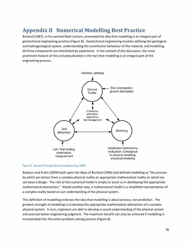
78

Appendix II Numerical Modelling Best Practice Burland (1987), in his seminal Nash Lecture, presented the idea that modelling is an integral part of

geotechnical engineering practice (Figure 8). Geotechnical engineering involves defining the geological

and hydrogeological system, understanding the constitutive behaviour of the material, and modelling.

All three components are interlinked by experience. In the context of this discussion, the most

prominent feature of this conceptualization is the fact that modelling is an integral part of the

engineering process.

Figure 8. Burland Triangle (Ground Engineering, 1996).

Barbour and Krahn (2004) built upon the ideas of Burland (1996) and defined modelling as “the process

by which we extract from a complex physical reality an appropriate mathematical reality on which we

can base a design. The role of the numerical model is simply to assist us in developing the appropriate

mathematical abstraction.” Stated another way, a mathematical model is a simplified representation of

a complex reality based on our understanding of the physical system.

This definition of modelling endorses the idea that modelling is about process, not prediction. The

greatest strength of modelling is to develop the appropriate mathematical abstraction of a complex

physical system. In turn, engineers are able to develop a sound understanding of the physical system

and exercise better engineering judgment. The maximum benefit can only be achieved if modelling is

incorporated into the entire problem solving process (Figure 8).

79

A finite element analysis is just one type of numerical model that is less restrictive and complimentary to

other types of numerical models, such as analytical and graphical solutions. The primary reason for

invoking a finite element analysis is to cope with various complexities, including: a) intricate geological

and hydrogeological settings; b) nontrivial physical processes; c) multiple and competing design

alternatives and economic implications; and, d) a decision making process that can be made difficult by

the need to communicate ideas to regulators and the general public.

Barbour and Krahn (2004) elaborate on some of the intricacies of each of these complexities. It is

perhaps worth highlighting that engineering problems involving the earth are particularly complicated

because natural systems exhibit extreme spatial variability, complex and sometimes unquantifiable

material behavior, incongruent temporal and spatial scales, and in many cases, physical processes that

are not fully understood. Barbour and Krahn (2004) illustrate this realization with a poignant case

history involving a comparison of various numerical simulations to measured deflections of a structurally

supported retaining wall for a deep excavation. None of the predictions of the lateral deflections were

accurate, or true to the measurements.

The reasons for the inaccuracies were related in part to the aforementioned complexities and

conceptualization errors, and in part to numerical problems. One can conclude that, in general,

predicting the exact response of a physical system is not feasible because it is impossible to reproduce

all of the detail present in the physical problem in even the most refined mathematical model.

Prediction should therefore not be the primary objective of numerical modelling. The encouraging

aspect of the case history was that the overall patterns of the physical behaviour were adequately

simulated. As such, the numerical solutions provided an appropriate basis for design.

This short discourse brings us back to the key advantage of numerical modelling: the process of

numerical modelling enhances engineering judgement and provides a basis for understanding

complicated physical processes. The process of modelling is iterative and comprises at least four

essential components:

1. Define the modelling objective and develop a conceptual model of the problem;

2. Determine the appropriate theoretical models (i.e., physics) that describe the key physical

processes;

3. Develop a mathematical description of these processes and verify that it provides an accurate

solution; and,

4. Interpret the results in relation to the observed physical reality.

Defining the modelling objective and developing a conceptual model are the most important steps in

the modelling process. Again, this is where numerical modelling can be exceptionally useful, as the

process forces the analyst to incorporate information on site geology and hydrogeology, laboratory

information, and any other pertinent information (e.g., construction sequencing) into a conceptual

model of the problem. The conceptual model must also be linked with the objectives of the modelling

exercise.

80

Determining the appropriate theoretical model involves gaining an understanding of the underlying

physics and the constitutive behavior governing material behavior. From the analysts’ perspective, this

is tantamount to ensuring that the formulation of the numerical model is representative of the physical

process being explored. This understanding is manifest in a model’s development through the definition

of the boundary conditions and material properties. These components often change as the analyst

iterates through the modelling process; refining the model as the understanding of the physical system

evolves and additional field and laboratory data becomes available.

Eventually, the conceptual and theoretical models are committed to a mathematical solution. In a finite

element analysis, the geometry of the problem domain is drawn, material properties are defined, and

boundary conditions are applied to the domain. A verification of the solution is completed to ensure

convergence, appropriate spatial and temporal discretization, and correct application of physics

(perhaps via comparison with an analytical solution). A simple to complex mantra must be adopted, so

that the analyst can be confident in the numerical solution.

Finally, the results are interpreted within the context of the physical reality. The most fundamental

question that should always be asked is: are the results reasonable? Stated another way, interpretation

of the results should be done with a skeptical mind-set. The results of the finite element analysis could

be compared with field monitoring data and should always be interpreted in light of the information

used to develop the conceptual and theoretical models.

A numerical model will likely evolve repeatedly over the course of the modelling process as the analyst

is challenged by interpreting the results. Increasing complexity of the conceptual model may be

required; however, speculating on high degrees of complexity in the absence of supporting observations

is not just problematic, it makes the remaining parts of the process more difficult or impossible. The

best numerical models include just enough complexity for the mathematical abstraction to reasonably

approximate the physical reality.

copyright © 2004-2018 by geoslope international,...

Documents