copyright © 2005 elsevier chapter 15:: code improvement programming language pragmatics michael l....

Copyright © 2005 Elsevier

Chapter 15:: Code Improvement

Programming Language PragmaticsMichael L. Scott


Introduction

• We discussed the generation, assembly, and linking of target code in the back end of a compiler– We get correct but highly suboptimal code

• redundant computations

• inefficient use of the registers, multiple functional units, and cache

• This chapter takes a look at code improvement: the phases of compilation devoted to generating good code– we interpret “good” to mean fast

– occasionally we also consider program transformations to decrease memory requirements


Introduction

• In a very simple compiler, we can use a peephole optimizer to peruse already-generated target code for obviously suboptimal sequences of adjacent instructions

• At a slightly higher level, we can generate near-optimal code for basic blocks– a basic block is a maximal-length sequence of instructions that

will always execute in its entirety (assuming it executes at all)

– in the absence of hardware exceptions, control never enters a basic block except at the beginning, and never exits except at the end


Introduction

• Code improvement at the level of basic blocks is known as local optimization– elimination of redundant operations (unnecessary loads, common sub-

expression calculations)

– effective instruction scheduling and register allocation

• At higher levels of aggressiveness, compilers employ techniques that analyze entire subroutines for further speed improvements

• These techniques are known as global optimization– multi-basic-block versions of redundancy elimination

– instruction scheduling, and register allocation

– code modifications designed to improve the performance of loops


Introduction

• Both global redundancy elimination and loop improvement typically employ a control flow graph representation of the program– Use a family of algorithms known as data flow analysis

(flow of information between basic blocks)

• Recent compilers perform various forms of interprocedural code improvement

• Interprocedural improvement is difficult– subroutines may be called from many different places

• hard to identify available registers, common subexpressions, etc.

– subroutines are separately compiled


Phases of Code Improvement

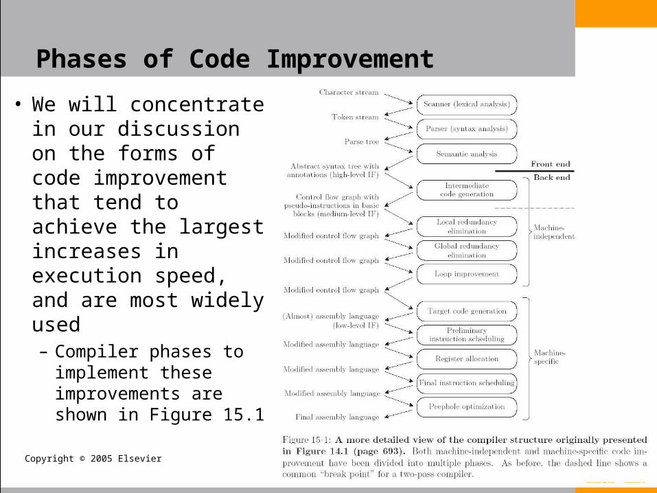
• We will concentrate in our discussion on the forms of code improvement that tend to achieve the largest increases in execution speed, and are most widely used– Compiler phases to

implement these improvements are shown in Figure 15.1



• The machine-independent part of the back end begins with intermediate code generation– identifies fragments of the syntax tree that correspond to

basic blocks

– creates a control flow graph in which each node contains a sequence of three-address instructions for an idealized machine (unlimited supply of virtual registers)

• The machine-specific part of the back end begins with target code generation– strings the basic blocks together into a linear program

• translates each block into the instruction set of the target machine and generating branch instructions that correspond to the arcs of the control flow graph



• Machine-independent code improvement has three separate phases1. Local redundancy elimination: identifies and

eliminates redundant loads, stores, and computations within each basic block

2. Global redundancy elimination: identifies similar redundancies across the boundaries between basic blocks (but within the bounds of a single subroutine)

3. Loop improvement: effects several improvements specific to loops• these are particularly important, since most programs spend

most of their time in loops.

• Global redundancy elimination and loop improvement may actually be subdivided into several separate phases



• Machine-specific code improvement has four separate phases– Preliminary and final instruction scheduling are essentially

identical (Phases 1 & 3)

– Register allocation (Phase 2) and instruction scheduling tend to interfere with one another• the instruction schedules minimize pipeline stalls which tend to

increase the demand for architectural registers (register pressure)

• we schedule instructions first, then allocate architectural registers, then schedule instructions again– If it turns out that there aren’t enough architectural registers, the

register allocator will generate additional load and store instructions to spill registers temporarily to memory

– the second round of instruction scheduling attempts to fill any delays induced by the extra loads


Peephole Optimization

• A relatively simple way to significantly improve the quality of naive code is to run a peephole optimizer over the target code– works by sliding a several instruction window (a

peephole) over the target code, looking for suboptimal patterns of instructions

– the patterns to look for are heuristic• patterns to match common suboptimal idioms produced by a

particular front end

• patterns to exploit special instructions available on a given machine

• A few examples are presented in what follows



• Elimination of redundant loads and stores– The peephole optimizer can often recognize that the

value produced by a load instruction is already available in a registerr2 := r1 + 5i := r2r3 := ir3 := r3 × 3

becomesr2 := r1 + 5i := r2r3 := r2 × 3



• Constant folding

• A naive code generator may produce code that performs calculations at run time that could actually be performed at compile time– A peephole optimizer can often recognize such

code

r2 := 3 × 2

becomes

r2 := 6



• Constant propagation– Sometimes we can tell that a variable will have a constant value at

a particular point in a program– We can then replace occurrences of the variable with occurrences

of the constantr2 := 4r3 := r1 + r2r2 := . . .

becomesr2 := 4r3 := r1 + 4r2 := . . .

and then r3 := r1 + 4r2 := . . .



• Common subexpression elimination– When the same calculation occurs twice within the

peephole of the optimizer, we can often eliminate the second calculation:r2 := r1 × 5r2 := r2 + r3r3 := r1 × 5

becomesr4 := r1 × 5r2 := r4 + r3r3 := r4

– Often, as shown here, an extra register will be needed to hold the common value



• It is natural to think of common subexpressions as something that could be eliminated at the source code level, and programmers are sometimes tempted to do so

• The following, for example,x = a + b + c;y = a + b + d;

could be replaced witht = a + b;x = t + c;y = t + d;



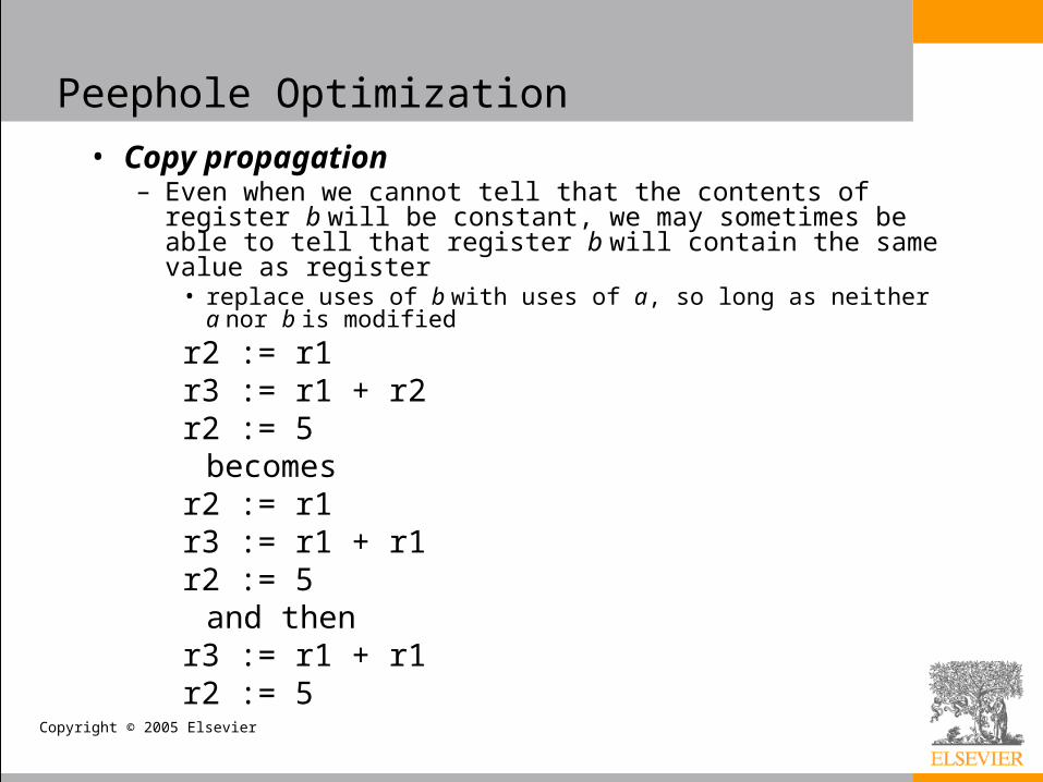
• Copy propagation– Even when we cannot tell that the contents of register b will be

constant, we may sometimes be able to tell that register b will contain the same value as register

• replace uses of b with uses of a, so long as neither a nor b is modified

r2 := r1r3 := r1 + r2r2 := 5

becomesr2 := r1r3 := r1 + r1r2 := 5

and then r3 := r1 + r1r2 := 5



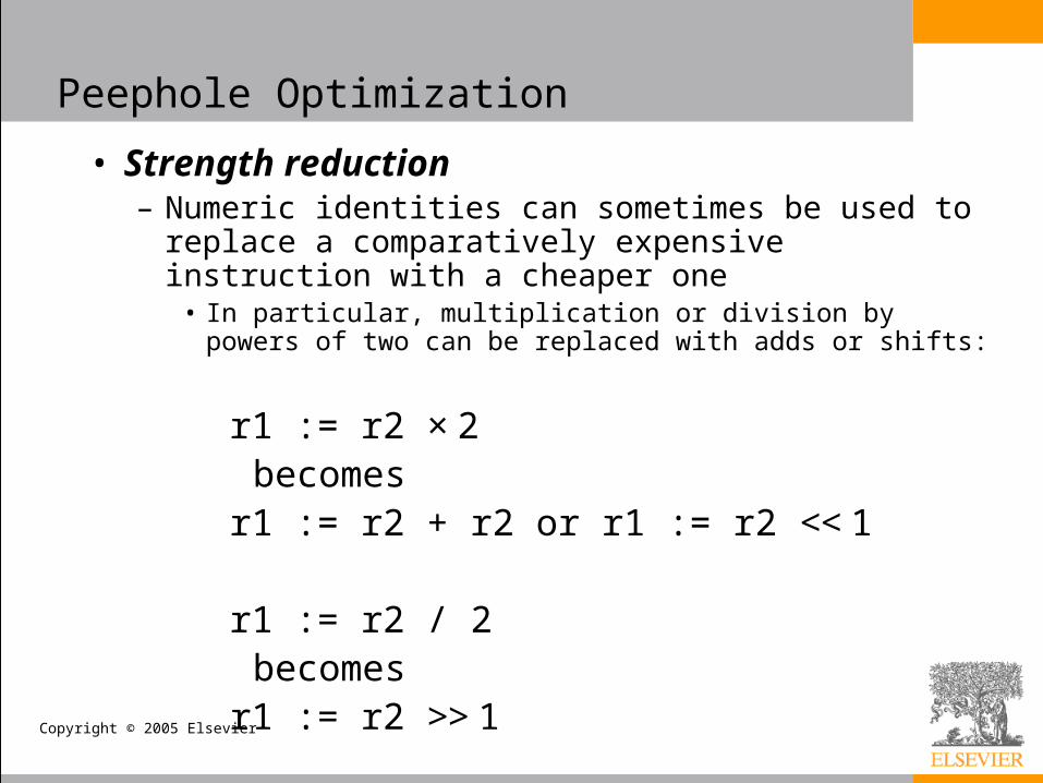
• Strength reduction– Numeric identities can sometimes be used to replace a

comparatively expensive instruction with a cheaper one• In particular, multiplication or division by powers of two can be

replaced with adds or shifts:

r1 := r2 × 2 becomes

r1 := r2 + r2 or r1 := r2 << 1

r1 := r2 / 2 becomes

r1 := r2 >> 1



• Elimination of useless instructions– Instructions like the following can be dropped

entirely:

r1 := r1 + 0r1 := r1 × 1

• Filling of load and branch delays– Several examples of delay-filling transformations

were presented in Chapter 5

• Exploitation of the instruction set– Particularly on CISC machines, sequences of

simple instructions can often be replaced by a smaller number of more complex instructions


Redundancy Elimination in Basic Blocks

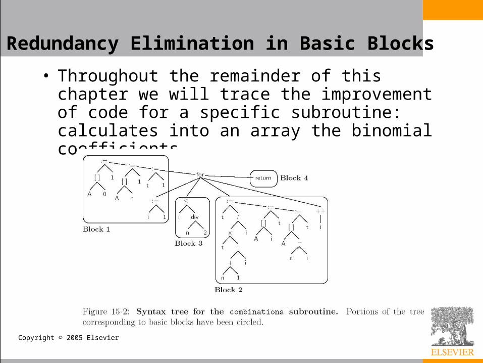
• Throughout the remainder of this chapter we will trace the improvement of code for a specific subroutine: calculates into an array the binomial coefficients



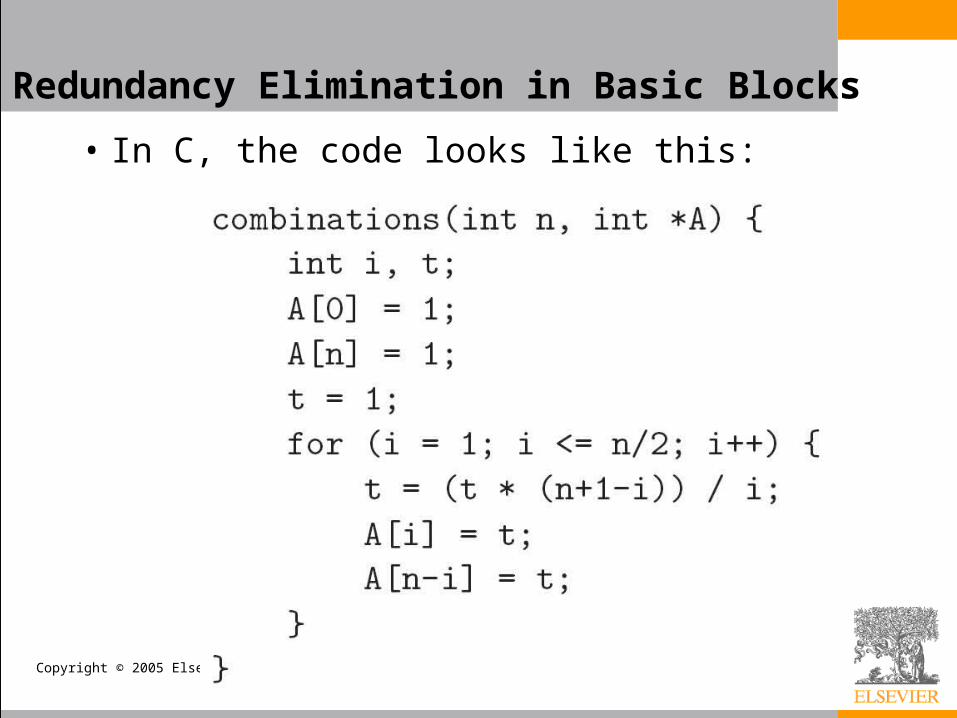
• In C, the code looks like this:



• We employ a medium level intermediate form (IF) for control flow– every calculated value is

placed in a separate register

– To emphasize virtual registers (of which there is an unlimited supply), we name them v1, v2, . . .

– We use r1, r2, . . . to represent architectural registers in Section 15.8.



• To improve the code within basic blocks, we need to– minimize loads and stores– identify redundant calculations

• There are two techniques usually employed1. translate the syntax tree for a basic block into an

expression DAG (directed acyclic graph) in which redundant loads and computations are merged into individual nodes with multiple parents

2. similar functionality can also be obtained without an explicitly graphical program representation, through a technique known as local value numbering

• We describe the last technique below



• Value numbering assigns the same name (a “number”) to any two or more symbolically equivalent computations (“values”), so that redundant instances will be recognizable by their common name

• Our names are virtual registers, which we merge whenever they are guaranteed to hold a common value

• While performing local value numbering, we will also implement – local constant folding– constant propagation, copy propagation– common subexpression elimination– strength reduction– useless instruction elimination


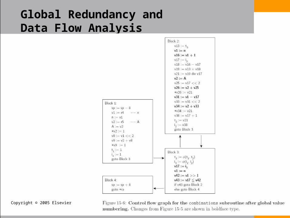
Global Redundancy and Data Flow Analysis

• We now concentrate on the elimination of redundant loads and computations across the boundaries between basic blocks

• We translate the code of our basic blocks into static single assignment (SSA) form, which will allow us to perform global value numbering

• Once value numbers have been assigned, we shall be able to perform – global common subexpression elimination– constant propagation– copy propagation



• In a compiler both the translation to SSA form and the various global optimizations would be driven by data flow analysis.– We detail the problems of identifying

• common subexpressions• useless store instructions

– We will also give data flow equations for the calculation of reaching definitions, used to move invariant computations out of loops

• Global redundancy elimination can be structured in such a way that it catches local redundancies as well, eliminating the need for a separate local pass



• Value numbering, as introduced earlier, assigns a distinct virtual register name to every symbolically distinct value that is loaded or computed in a given body of code– It allows us to recognize when certain loads or

computations are redundant.

• The first step in global value numbering is to distinguish among the values that may be written to a variable in different basic blocks– We accomplish this step using static single assignment

(SSA) form



• For example, if the instruction v2 := x is guaranteed to read the value of x written by the instruction x3 := v1, then we replace v2 := x with v2 := x3

• If we cannot tell which version of x will be read, we use a hypothetical function φ to choose among the possible alternatives– we won’t actually have to compute φ-functions at run

time• the only purpose is to help us identify possible code

improvements

– we will drop them (and the subscripts) prior to target code generation


• With flow-dependent values determined by φ-functions, we are now in a position to perform global value numbering– As in local value numbering, the goal is to merge any

virtual registers that are guaranteed to hold symbolically equivalent expressions

– In the local case, we were able to perform a linear pass over the code

– We kept a dictionary that mapped loaded and computed expressions to the names of virtual registers that contained them



• This approach does not suffice in the global case, because the code may have cycles– The general solution can be formulated using data flow– It can also be obtained with a simpler algorithm that

begins by unifying all expressions with the same top-level operator• In the end, repeatedly separates expressions whose operands

are distinct• It is quite similar to the DFA minimization algorithm of

Chapter 2

• We perform this analysis for our running example informally



• Many instances of data flow analysis can be cast in the following framework: 1. four sets for each basic block B, called InB, OutB, GenB,

and KillB; 2. values for the Gen and Kill sets; 3. an equation relating the sets for any given block B; 4. an equation relating the Out set of a given block to the

In sets of its successors, or relating the In set of the block to the Out sets of its predecessors; and (often)

5. certain initial conditions



• The goal of the analysis is to find a fixed point of the equations: a consistent set of In and Out sets (usually the smallest or the largest) that satisfy both the equations and the initial conditions– Some problems have a single fixed point

– Others may have more than one• we usually want either the least or the greatest fixed point

(smallest or largest sets)



• In the case of global common subexpression elimination, InB is the set of expressions (virtual registers) guaranteed to be available at the beginning of block B– These available expressions will all have been set by

predecessor blocks– OutB is the set of expressions guaranteed to be

available at the end of B– KillB is the set of expressions killed in B: invalidated by

assignment to one of the variables used to calculate the expression, and not subsequently recalculated in B

– GenB is the set of expressions calculated in B and not subsequently killed in B



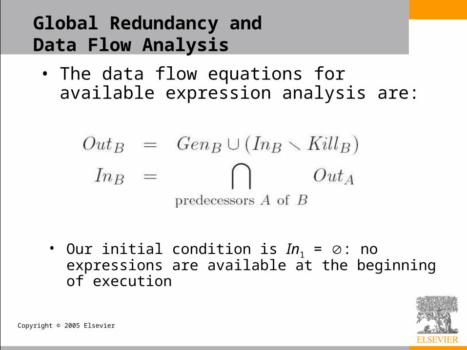
• The data flow equations for available expression analysis are:


• Our initial condition is In1 = : no expressions are available at the beginning of execution


• Available expression analysis is known as a forward data flow problem, because information flows forward across branches: the In set of a block depends on the Out sets of its predecessors– We will see an example of a backward data flow

problem later

• We calculate the desired fixed point of our equations in an inductive (iterative) fashion, much as we computed first and follow sets in Chapter 2

• Our equation for InB uses intersection to insist that an expression be available on all paths into B– In our iterative algorithm, this means that InB can only

shrink with subsequent iterations



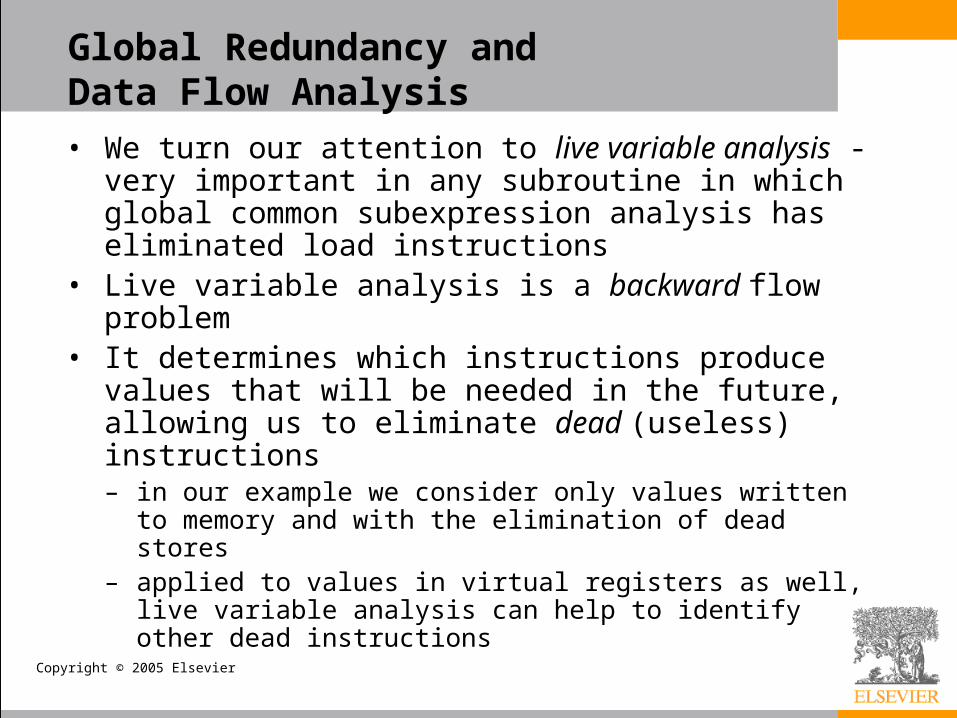
• We turn our attention to live variable analysis -very important in any subroutine in which global common subexpression analysis has eliminated load instructions

• Live variable analysis is a backward flow problem• It determines which instructions produce values

that will be needed in the future, allowing us to eliminate dead (useless) instructions– in our example we consider only values written to

memory and with the elimination of dead stores– applied to values in virtual registers as well, live variable

analysis can help to identify other dead instructions



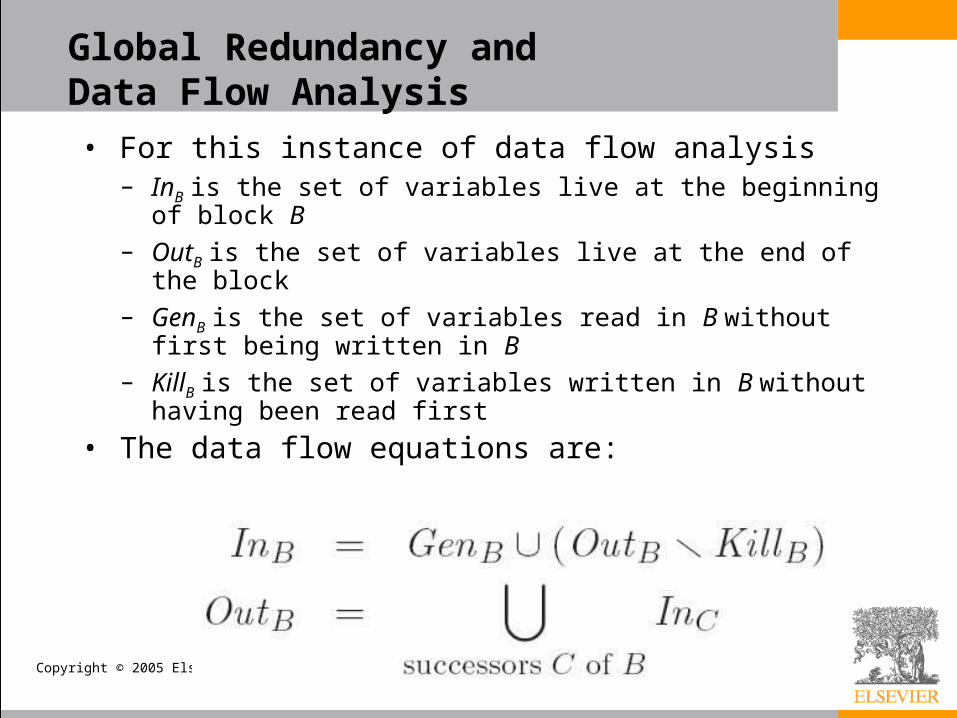
• For this instance of data flow analysis– InB is the set of variables live at the beginning of block B– OutB is the set of variables live at the end of the block– GenB is the set of variables read in B without first being

written in B– KillB is the set of variables written in B without having

been read first

• The data flow equations are:



• We consider two classes of loop improvements: – those that move invariant computations out of the body

of a loop and into its header, and– those that reduce the amount of time spent maintaining

induction variables

• Later we consider transformations that improve instruction scheduling by restructuring a loop body to include portions of more than one iteration of the original loop– manipulate multiply nested loops to improve cache

performance or increase opportunities for parallelization

Loop Improvement I


• A loop invariant is an instruction (i.e., a load or calculation) in a loop whose result is guaranteed to be the same in every iteration– If a loop is executed n times and we are able to move

an invariant instruction out of the body and into the header (saving its result in a register for use within the body), then we will eliminate n -1 calculations from the program• a potentially significant savings

• In order to tell whether an instruction is invariant, we need to identify the bodies of loops, and we need to track the locations at which operand values are defined

Loop Improvement I


• Tracking the locations at which an operand may have been defined amounts to the problem of reaching definitions– Formally, we say an instruction that assigns a value v

into a location (variable or register) l reaches a point p in the code if v may still be in l at p

• Like the conversion to static single assignment form, considered informally earlier, the problem of reaching definitions can be structured as a set of forward, any-path data flow equations– We let GenB be the set of final assignments in block B

(those that are not overwritten later in B)– For each assignment in B we also place in KillB all other

assignments (in any block) to the same location

Loop Improvement I


• Then we have

Loop Improvement I

• Given InB (the set of reaching definitions at the beginning of the block), we can determine the reaching definitions of all values used within B by a simple linear perusal of the code


Loop Improvement I


• An induction variable (or register) is one that takes on a simple progression of values in successive iterations of a loop. – We confine our attention to arithmetic progressions– Induction variables appear as loop indices, subscript

computations, or variables incremented or decremented explicitly within the body of the loop

• Induction variables are important for two reasons:– They commonly provide opportunities for strength

reduction, replacing multiplication with addition– They are commonly redundant: instead of keeping

several induction variables in registers, we can often keep a smaller number and calculate the remainder from those when needed

Loop Improvement I


Loop Improvement I


• We will perform two rounds of instruction scheduling separated by register allocation– Given our use of pseudoassembler, we won’t consider

peephole optimization in any further detail – On a pipelined machine, performance depends

critically on the extent to which the compiler is able to keep the pipeline full• A compiler can solve the subproblem of filling branch delays

in a more or less straightforward fashion

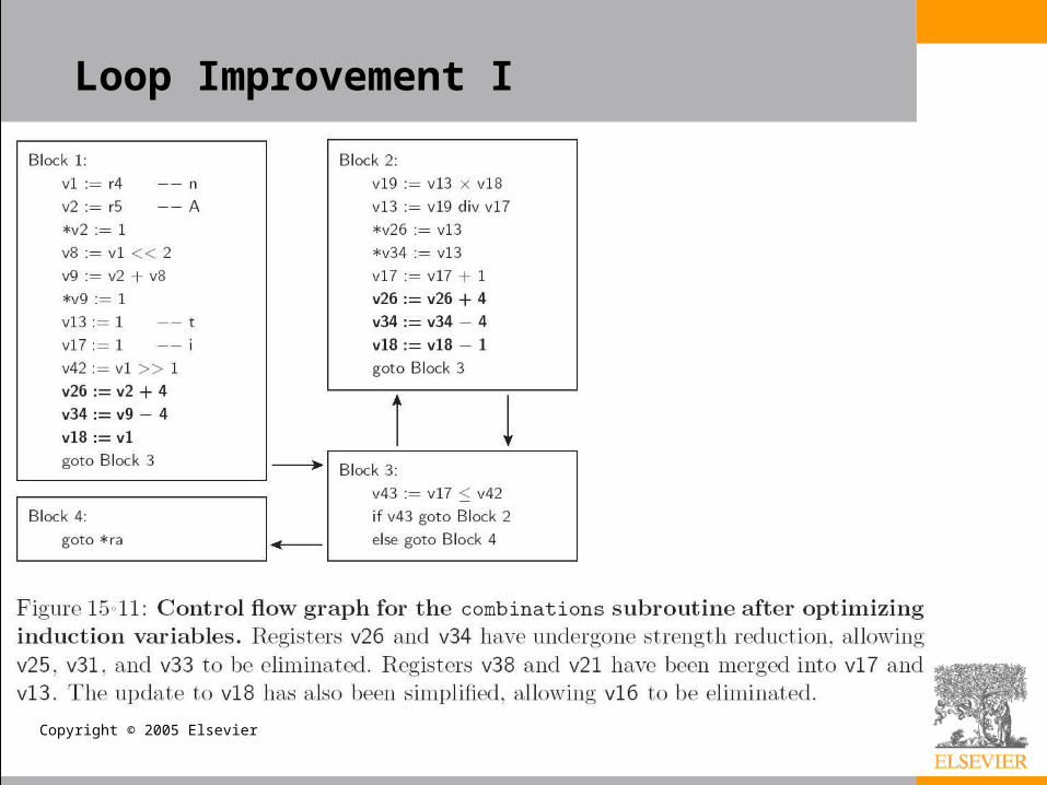
– If we examine the body of the loop in our combinations example, optimizations described thus far have transformed Block 2 from the 30 instruction sequence into the eight instruction sequence of Figure 15.11 • Unfortunately, on a pipelined machine without instruction

reordering, this code is still distinctly suboptimal

Instruction Scheduling


• To schedule instructions to make better use of the pipeline, we first arrange them into a directed acyclic graph (DAG), in which each node represents an instruction, and each arc represents a dependence– Most arcs will represent flow dependences, in which

one instruction uses a value produced by a previous instruction

– A few will represent anti-dependences, in which a later instruction overwrites a value read by a previous instruction

– In our example, these will correspond to updates of induction variables



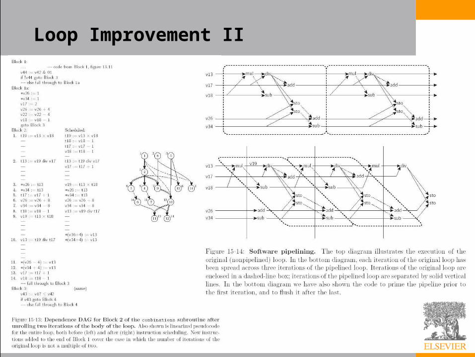
Loop Unrolling and Software Pipelining• Loop unrolling is a transformation that embeds

two or more iterations of a source-level loop in a single iteration of a new, longer loop, and allowing the scheduler to intermingle the instructions of the original iterations

• If we unroll two iterations of our combinations example we obtain the code of Figure 15.13– We have used separate names (here starting with the

letter ‘t’) for registers written in the initial half of the loop

– This convention minimizes anti- and output dependences, giving us more latitude in scheduling

Loop Improvement II


Loop Improvement II


• A software-pipelined version of our combinations subroutine appears in the bottom half of Figure 15.14 and as a control flow graph in Figure 15.15– The idea is to build a loop whose body comprises

portions of several consecutive iterations of the original loop, with no internal start-up or shut-down cost

– In our example, each iteration of the software-pipelined loop contributes to three separate iterations of the original loop

– Within each new iteration (shown between vertical bars) nothing needs to wait for the divide to complete

– To avoid delays, we have altered the code in several ways

Loop Improvement II


Loop Improvement II


Loop Improvement II

Loop Reordering

• The code improvement techniques that we have considered thus far have served two principal purposes– eliminate redundant or unnecessary instructions

– minimize stalls on a pipelined machine.

• Two other goals have become increasingly important in recent years– it has become increasingly important to minimize cache misses

(processor speed outstrips memory latency)

– it has become important to identify sections of code that can execute concurrently (parallel machines)

• As with other optimizations, the largest benefits come from changing the behavior of loops


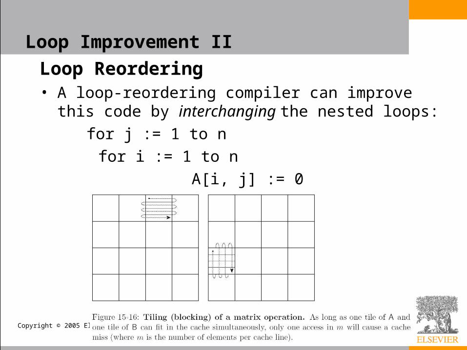
Loop Improvement II

Loop Reordering• A loop-reordering compiler can improve this code by

interchanging the nested loops:

for j := 1 to n

for i := 1 to n

A[i, j] := 0


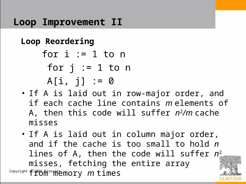
Loop Improvement II

Loop Reordering

for i := 1 to n

for j := 1 to n

A[i, j] := 0• If A is laid out in row-major order, and if each cache

line contains m elements of A, then this code will suffer n2/m cache misses

• If A is laid out in column major order, and if the cache is too small to hold n lines of A, then the code will suffer n2 misses, fetching the entire array from memory m times


Loop Improvement II

Loop Dependences• When reordering loops, we must to respect all data

dependences (loop-carried dependences)

i := 2 to n

for j := 1 to n1

A[i, j] := A[i, j] A[i1, j+1]

• Here the calculation of A[i, j] in iteration (i, j) depends on the value of A[i-1, j+1], which was calculated in iteration (i-1, j+1).

• This dependence is often represented by a diagram of the iteration space (see next slide):


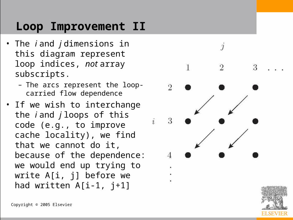
Loop Improvement II

• The i and j dimensions in this diagram represent loop indices, not array subscripts. – The arcs represent the loop-carried

flow dependence

• If we wish to interchange the i and j loops of this code (e.g., to improve cache locality), we find that we cannot do it, because of the dependence: we would end up trying to write A[i, j] before we had written A[i-1, j+1]


Loop Improvement II

• By analyzing the loop dependence, we note that we can reverse the order of the j loop without violating the dependence:

for i := 2 to n

for j := n1 to 1 by 1

A[i, j] := A[i, j] A[i1, j+1]

• This change transforms the iteration space as shown here


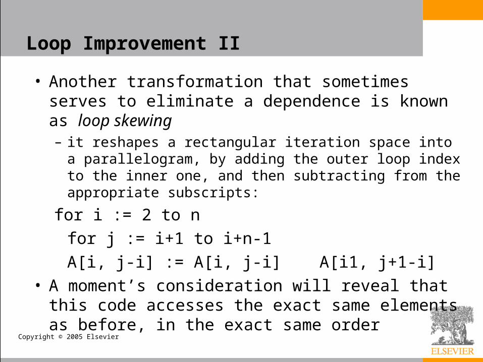
Loop Improvement II

• Another transformation that sometimes serves to eliminate a dependence is known as loop skewing– it reshapes a rectangular iteration space into a

parallelogram, by adding the outer loop index to the inner one, and then subtracting from the appropriate subscripts:

for i := 2 to n

for j := i+1 to i+n-1

A[i, j-i] := A[i, j-i] A[i1, j+1-i]

• A moment’s consideration will reveal that this code accesses the exact same elements as before, in the exact same order


Loop Improvement II

• Its iteration space, however, looks like here (the loops can be safely be interchanged)


Loop Improvement II

Parallelization• Loop iterations (at least in non-recursive programs)

constitute the principal source of operations that can execute in parallel– one needs to find independent loop iterations - with no

loop-carried dependences

• Even in languages without special constructs, a compiler can often parallelize code by identifying—or creating—loops with as few loop-carried dependences as possible– These transformations are valuable tools in this endeavor


Loop Improvement II

• Consider the problem of “zero-ing out” a two-dimensional array (row-major order):for i := 0 to n-1

for j := 0 to n-1

A[i, j] := 0

• On a machine containing several general purpose processors, we parallelize the outer loop:

–– on processor pid:

for i := (n/p × pid) to (n/p ×(pid + 1)-1)

for j := 1 to n

A[i, j] := 0


Loop Improvement II

• Other issues of importance in parallelizing compilers include communication and load balance

• Locality in parallel programs reduces communication among processors and between the processors and memory– Optimizations similar to those employed to reduce the number of

cache misses on a uniprocessor can be used to reduce communication trafic on a multiprocessor.

• Load balance refers to the division of labor among processors on a parallel machine– dividing a program among 16 processors, we shall obtain a speedup

of close to 16 only if each processor takes the same amount of time to do its work

– assigning 5% of the work to each of 15 processors and 25% of the work to the sixteenth, we are likely to see a speedup of no more than four


Register Allocation

• In a simple compiler with no global optimizations, register allocation can be performed independently in every basic block– simple compilers usually apply a set of heuristics to

identify such frequently accessed variables variables and allocate them to registers over the life of a subroutine.

– candidates for a dedicated register include loop indices, the implicit pointers of with statements in Pascal-family languages, and scalar local variables and parameters

• It has been known since the early 1970s that register allocation is equivalent to the NP-hard problem of graph coloring


Register Allocation

• We first identify virtual registers that cannot share an architectural register, because they contain values that are live concurrently– we use reaching definitions data flow analysis

– we then determine the live range of variables

• Given these live ranges, we construct a register interference graph– The nodes of this graph represent virtual registers.

Registers vi and vj are connected by an arc if they are simultaneously live

– The interference graph corresponding to Figure 15.17 appears in Figure 15.18 (see next slides)


Register Allocation

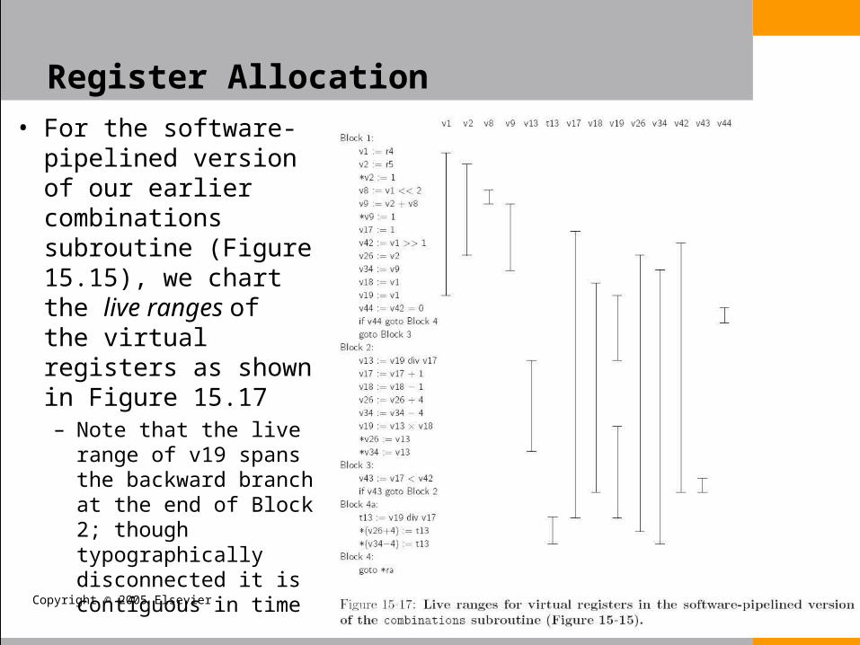
• For the software-pipelined version of our earlier combinations subroutine (Figure 15.15), we chart the live ranges of the virtual registers as shown in Figure 15.17– Note that the live range

of v19 spans the backward branch at the end of Block 2; though typographically disconnected it is contiguous in time


Register Allocation


Register Allocation

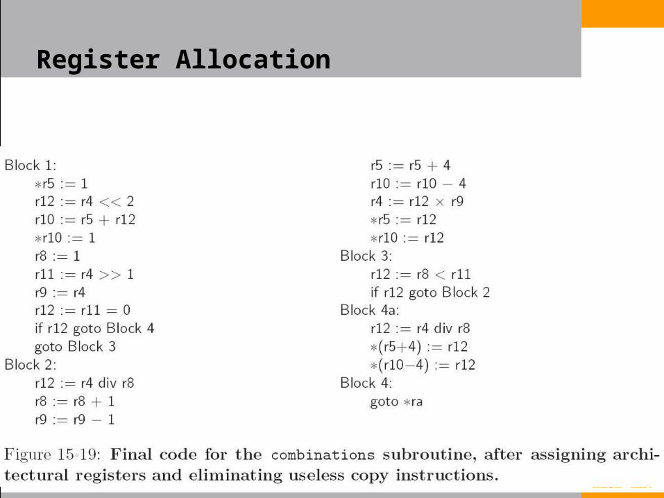
• The problem of mapping virtual registers onto the smallest possible number of architectural registers now amounts to finding a minimal coloring of this graph - an assignment of “colors” to nodes such that no arc connects two nodes of the same color

• In our example, we can find one of several optimal solutions by inspection– note that the six registers in the center of the figure

constitute a clique (a completely connected subgraph); each must be mapped to a separate architectural register

– final code for the combinations subroutine appears in Figure 15.19


Register Allocation

copyright © 2005 elsevier chapter 15:: code improvement programming language pragmatics michael l....

Documents

forms of code improvement

generated target code

target code generationstrings

basic blocksa basic

basic blockscreates

target machine

level of basic blocks

basic blocksrecent compilers