©Copyright 2020

Andrew M. Pace

Stepping Towards Control of Systems Undergoing Impact for

Legged Locomotion

Andrew M. Pace

A dissertationsubmitted in partial fulfillment of the

requirements for the degree of

Doctor of Philosophy

University of Washington

2020

Reading Committee:

Samuel A. Burden, Chair

Aleksandr Aravkin

J. Nathan Kutz

Michael T. Brett, GSR

Program Authorized to Offer Degree:Electrical Engineering

University of Washington

Abstract

Stepping Towards Control of Systems Undergoing Impact for Legged Locomotion

Andrew M. Pace

Chair of the Supervisory Committee:Dr. Samuel A. BurdenElectrical Engineering

This dissertation focuses on bringing control theory to mechanical systems subject to uni-

lateral constraints, with the focus on legged locomotion. The key feature of these systems is

the impact that occurs, causing a sudden change in the velocity of the object and a potential

change in its underlying vector fields. The primary challenge for such systems arises from

constraint activation, in other words, when a leg transitions from moving through the air to

the ground. Throughout this dissertation, the dynamics are captured using the modelling

paradigm of hybrid dynamical systems. In the language of hybrid dynamical systems, a

reset occurs causing instantaneous change in the systems velocity. In addition, when a con-

straint activates or deactivates, the underlying vector field discontinuously changes. Such

discontinuities violate continuity and smoothness assumptions many classical control tech-

niques impose. This dissertation focuses on developing three aspects of control for legged

locomotion: developing a control law about a desired trajectory undergoing simultaneous

constrain activations, such as a pronk gait, determining the complete state, both discrete

and continuous, of the system from noisy measurements, and finding a control law to track

a desired trajectory through contact.

TABLE OF CONTENTS

Page

List of Figures . . . . . . . . . . . . . . . . . . . . . . . . . . . . . . . . . . . . . . . iii

List of Tables . . . . . . . . . . . . . . . . . . . . . . . . . . . . . . . . . . . . . . . . vi

Chapter 1: Introduction . . . . . . . . . . . . . . . . . . . . . . . . . . . . . . . . 1

1.1 A brief overview of rigid mechanical systems modeled as Hybrid DynamicalSystems . . . . . . . . . . . . . . . . . . . . . . . . . . . . . . . . . . . . . . 2

1.2 Dissertation Content . . . . . . . . . . . . . . . . . . . . . . . . . . . . . . . 2

Chapter 2: Nonplastic Inelastic Billiards Must Have a new distance function . . . 4

2.1 Abstract . . . . . . . . . . . . . . . . . . . . . . . . . . . . . . . . . . . . . . 4

2.2 Introduction . . . . . . . . . . . . . . . . . . . . . . . . . . . . . . . . . . . . 4

2.3 Nonplastic Inelastic 1-DOF Billiard . . . . . . . . . . . . . . . . . . . . . . . 6

2.4 Discussion . . . . . . . . . . . . . . . . . . . . . . . . . . . . . . . . . . . . . 13

Chapter 3: State Estimation in Hybrid Dynamical Systems . . . . . . . . . . . . . 16

3.1 Abstract . . . . . . . . . . . . . . . . . . . . . . . . . . . . . . . . . . . . . . 16

3.2 Introduction . . . . . . . . . . . . . . . . . . . . . . . . . . . . . . . . . . . . 16

3.3 Problem formulation . . . . . . . . . . . . . . . . . . . . . . . . . . . . . . . 18

3.4 State estimation algorithm . . . . . . . . . . . . . . . . . . . . . . . . . . . . 24

3.5 Parameter Tuning for Proposed Algorithm . . . . . . . . . . . . . . . . . . . 31

3.6 Comparison with the Interacting Multiple Model (IMM) method . . . . . . . 32

3.7 Experiments with hybrid system models . . . . . . . . . . . . . . . . . . . . 35

3.8 Conclusion . . . . . . . . . . . . . . . . . . . . . . . . . . . . . . . . . . . . . 43

Chapter 4: Piecewise–differentiable flow . . . . . . . . . . . . . . . . . . . . . . . . 45

4.1 Abstract . . . . . . . . . . . . . . . . . . . . . . . . . . . . . . . . . . . . . . 45

4.2 Introduction . . . . . . . . . . . . . . . . . . . . . . . . . . . . . . . . . . . . 45

i

4.3 Background . . . . . . . . . . . . . . . . . . . . . . . . . . . . . . . . . . . . 46

4.4 Differentiability with differing contact mode sequences . . . . . . . . . . . . 59

4.5 Applications . . . . . . . . . . . . . . . . . . . . . . . . . . . . . . . . . . . . 72

4.6 Discussion . . . . . . . . . . . . . . . . . . . . . . . . . . . . . . . . . . . . . 79

Chapter 5: Discussion . . . . . . . . . . . . . . . . . . . . . . . . . . . . . . . . . . 91

Bibliography . . . . . . . . . . . . . . . . . . . . . . . . . . . . . . . . . . . . . . . . 93

Appendix A: Appendices for Chapter 3 . . . . . . . . . . . . . . . . . . . . . . . . . 103

A.1 Switched and hybrid dynamical systems . . . . . . . . . . . . . . . . . . . . 103

A.2 Linear Spring Double Mass Hopper . . . . . . . . . . . . . . . . . . . . . . . 104

A.3 Nonlinear double mass hopper hybrid system description . . . . . . . . . . . 106

A.4 With measurement model Hrelative, the linear one foot robot described in 3.7.2is unobservable. . . . . . . . . . . . . . . . . . . . . . . . . . . . . . . . . . . 106

ii

LIST OF FIGURES

Figure Number Page

2.1 A graphical representation of a trajectory in TC. The arrows indicate thedirection of travel with increasing time t. . . . . . . . . . . . . . . . . . . . . 7

2.2 An example trajectory in TC. . . . . . . . . . . . . . . . . . . . . . . . . . . 9

2.3 Visual representation of the projection P on two points in TC and their cor-responding points in TC(top) and for a trajectory (bottom). . . . . . . . . 10

2.4 A visual representation of function d compatible with d under P , (top) when

both points are in TC+ (bottom) when both points are in TC−. . . . . . . . 12

2.5 Assuming a function d:TC×TC → R+ is compatible with d, d cannotbe continuous and hence is not a distance function. with the desiredproperties of continuity and compatibility can not exist. The two sequences inTC, the semi-filled blue and green circles, converge to the filled blue and greencircles, yet with the distance measure d having the compatibility property thedistance on the convergent series does not equal the distance of the convergedpoints. . . . . . . . . . . . . . . . . . . . . . . . . . . . . . . . . . . . . . . 13

3.1 Probabability density and negative log-likelihood functions for Gaussian (solidblue) and Student’s t (dashed red; degree-of-freedom r = 1) distributions. . . 21

3.2 Algorithm 1 (VP) performs comparably to IMM when the contin-uous state does not undergo any resets. The top plot shows the truestate w and the simplex estimate of the true state from both methods wV P ,wIMM1 . The simplex estimate is shown in color and the probability estimateof the discrete state being w = 1 is superimposed as a black line. The middleplot shows the actual value of the continuous state of the simulation and theestimates. The bottom plot shows the residual between true continuous stateand the estimated continuous state. . . . . . . . . . . . . . . . . . . . . . . 34

3.3 Algorithm 1 (VP) outperforms the IMM when there are jumps inthe continuous state. The plots follow the convention laid out in Figure 3.2. 34

iii

3.4 Jumping robot and impact oscillator hybrid system models (Sec. 3.7.1).(a) Photograph of the physical robot (one leg from a Minitaur [52]) that in-spired the simulation models. (b) Nonlinear model consisting of two massescoupled with a linear spring and a nonlinear pantograph mechanism. (c) Lin-ear model consisting of two masses coupled with a linear spring. . . . . . . 36

3.5 The Student’s t distribution process noise yields better estimatesof instantaneous changes in continuous state (Sec. 3.7.2). In this plot,estimates of the foot velocity are shown near two impacts (≈ 16.6s, 17.5s). . 39

3.6 Gauss-Newton descent directions yield faster convergence than gra-dient (steepest) descent (Sec. 3.7.2). In this plot, the discrete state vari-ables w are given and the second line of Algorithm 1 is modified to use eitherGauss-Newton descent directions or gradient (steepest) descent to estimatethe continuous state variables x by minimizing the relaxed objective functionf(x,w) (3.6). . . . . . . . . . . . . . . . . . . . . . . . . . . . . . . . . . . . 40

3.7 Without smoothing (ν = 0), the discrete state estimate switchesfrequently (Sec. 3.7.2). With smoothing (ν > 0), the discrete stateestimate mostly switches near the true switching times. (Sec. 3.7.2).The top plot shows the true discrete state of the system w ∈ DM , the relaxeddiscrete state estimate w ∈ ∆M , and the discrete state estimate w ∈ DM fora simulation of the piecewise-linear system. The subsequent plots show theestimate, simulation, and error ε values for position and velocity of the hipq[1] and foot q[2]. . . . . . . . . . . . . . . . . . . . . . . . . . . . . . . . . 41

3.8 Estimated discrete state using onboard (relative position and ve-locity) measurements Hrelative (3.15) for the piecewise-linear systemclosely matches true discrete state. (Sec. 3.7.2). Continuous state esti-mates are not shown since they are formally unobservable using only onboardmeasurements (in practice, they drift away from ground truth over time). . . 42

3.9 State estimatotion for a piecewise-nonlinear model (Sec. 3.7.1); note the non-linear model only has two discrete states. . . . . . . . . . . . . . . . . . . . . 44

4.1 Figure of a basic example piecewise differentiable flow. The pictured systemis described in detail in section 4.5.1 . . . . . . . . . . . . . . . . . . . . . . 47

4.2 Example of what a constant contact mode sequence means for differentiationand why differentiable . . . . . . . . . . . . . . . . . . . . . . . . . . . . . . 52

4.3 Example of a discontinuous flow . . . . . . . . . . . . . . . . . . . . . . . . 57

iv

4.4 Illustration of trajectory undergoing simultaneous constraint activation anddeactivation: the trajectory initialized at (p, p) ∈ TA1 ⊂ TQ flows via (4.6a)to a point (ρ, ρ−) ∈ TA1 where both the constraint force λ1 and con-straint function a2 are zero, instantaneously resets velocity via (4.6b) to ρ+ =∆2(ρ)ρ−, then flows via (4.6a) to φ(t, (p, p)) ∈ TA2 ⊂ TQ. Nearby tra-jectories undergo activation and deactivation at distinct times: trajectoriesinitialized in the red region, e.g. (vr, vr), deactivate constraint 1 and flowthrough contact mode TA∅ before activating constraint 2—their contact modesequence is (1 , ∅, 2)—while trajectories initialized in the blue region, e.g.(vb, vb), activate 2 and flow through TA1,2 before deactivating 1—their con-tact mode sequence is (1 , 1, 2 , 2). Here, the constraint activation trig-gered a plastic impact wherein eq. (4.6b) resets the velocity normal to theactivated constraint to zero; if the activation had instead been elastic, thenthe final contact mode would have been TA∅. Note that constraint acti-vations generally reset the system state to the interior of a contact mode,whereas deactivations reset the system state to the boundary of a contactmode. Piecewise–differentiability of the trajectory outcome is illustrated bythe fact that red outcomes lie along a different subspace than blue. . . . . . 87

4.5 Trajectory outcomes in mechanical systems subject to unilateral constraints 88

4.6 PCr flow for the double pendulum . . . . . . . . . . . . . . . . . . . . . . . 89

4.7 Nonsmooth control law for a PCr system from . . . . . . . . . . . . . . . . . 90

v

LIST OF TABLES

Table Number Page

3.1 Discrete states and continuous dynamics for impact oscillator hybridsystem models (Sec. 3.7.1). Note that the continuous dynamics q have thesame general form for both the piecewise-linear and -nonlinear models, withthe spring law k being a linear or nonlinear function of the continuous statex = (q, q) depending on which model is considered. . . . . . . . . . . . . . . 38

4.1 Parameter values used in simulation to generate Fig. 4.5 . . . . . . . . . . . 77

4.2 Parameter values used in simulation to generate Fig. 4.6 . . . . . . . . . . . 78

vi

ACKNOWLEDGMENTS

The work of this dissertation, while mine, was never mine alone. I want to take this

opportunity who explicitly and implicitly played some role in completing this dissertation.

I will start with thanking my adviser, Professor Sam Burden, for the immense guidance

he gave, the continuous support, and the encouragement to look beyond existing tools and

techniques to come up with novel methods. Additionally, I want to thank the remainder of

my committee: Professor Sasha Aravkin, for showing me the development of an objective

function goes hand in hand with the optimization algorithm, Professor Nathan Kutz, for

making me think of how to make hybrid dynamics more widely used, and Professor Mike

Brett, for teaching me the French roll (and for taking the time to serve as GSR!).

Next, I want to thank my other collaborators Jize Zhang for tolerating the many itera-

tions of our paper’s figures, Rahul Malik 1 for patiently explaining how Dual Active Bridge

(DAB) converters works over and over again, and both for their immeasurable patience with

explaining new concepts.

The many people who have come through the ”Burden Group,” Bora Banjanin, Yana

Sosnovskaya, Momona Yamagami, Ben Chasnov, Joey Sullivan, Shruti Misra, Tianqi Li, and

Liam Han; to all of you, I am greatly indebted. Without our frequent conversations and chats

that go far beyond research, I may not have completed this dissertation. To the many people

both in and outside of BRL who have supported and encouraged me throughout this process,

Andy Lewis, Nava Agadhasi, Kevin Huang, Astrini Sie, Dianmu Zhang, David Caballero,

Vijeth Rai, Katherine Pratt, Sarah Li, Yohan Min, Gaurav Mukherjee, and all the members

1The work from the collaboration with Rahul unfortunately does not appear in this dissertation. Instead,it can be found in [69] and perhaps in a part Rahul’s future dissertation.

vii

of Seattle Cattle, I thank you; all of our conversations, from the general companionship to

the advice, helped me push through. I thank Brandon Larson and Jennifer Huberman for

advising me and helping me figure out all the necessary forms needed to actually graduate.

Additionally, I would like to thank the creators and contributors of NumPy [81, 104] and

Matplotlib [47], whose use was necessary for the computational examples throughout this

dissertation.

Finally, I thank my family. My parents for humoring me on this journey and their

unending support throughout my life. My sister for and bringing along Patch, who helped

me adjust to walking in the constant Seattle drizzle.

viii

1

Chapter 1

INTRODUCTION

In this dissertation I seek to solve of the challenges facing control of legged robots. The

challenge of such systems is the sudden change in velocity whenever a leg touches down,

particularly when running with legs of significant mass. Many current control techniques

for legged locomotion attempt to minimize or remove these discontinuities, either through

modeling (massless limbs, multi-level control such as templates and anchors [36]) or control

that minimizes impact velocity. As part of the goal of this dissertation, I seek to enable

control that at the model level does not require such workarounds.

Throughout this dissertation, I will be assuming the robot is made of rigid mechanical

components, neglecting the rich subfield of soft robotics. This assumption makes possible

the use of hybrid dynamical systems1 in a straightforward manner. Additionally, modeling

the physical system as a hybrid dynamical system, in particular a mechanical system subject

to unilateral constraints, captures the salient features of the real world dynamics. That is,

the flow of such models are left-continuous.2

Three critical components, but by no means the only critical component, of any closed

loop control system are tracking a reference, state estimation, and generating the control

signal. Classical control3 focuses on controlling continuous flows. For each of these three

problems, classical solution has several solutions for. While hybrid dynamics is not a new

field and has been used for control, most of the early motivation was for continuous systems

and later work seeks general control techniques for all hybrid dynamics. It is my view, much

1Also hybrid system or hybrid dynamics

2As will be briefly touched on in chapter 4, hybrid dynamics is but one modeling choice for such systems,complementarity and measure differential inclusion are two others.

3Which I lump so called modern control theory as part of.

2

can be gained by incorporating knowledge from mechanics into the control techniques. This

dissertation will not solve these challenges for legged robots but to provide feasible paths

forward.

1.1 A brief overview of rigid mechanical systems modeled as Hybrid Dynam-ical Systems

Before proceeding, I will provide an overview of the relevant portions of hybrid dynamics

as will be useful in this dissertation. See [39] for a general introduction to hybrid dynamics

and [50] for a more detailed account of modeling legged robots with hybrid dynamics. The

hybrid domain, which in this dissertation may sometimes be referred to as mode or discrete

state, indexes into the set of underlying vector fields. To account for this additional infor-

mation, I will refer to the state of a hybrid system as the continuous state and discrete state.

A guard is a set of sets within the hybrid domain specifies when the state change, either

the discrete or continuous or both change4 may change. For a legged robot, guard generally

correspond to when unilateral constraints are active, which is equal to zero. When a uni-

lateral constraint becomes active, an impact occurs which causes a jump in state’s velocity

such that the unilateral constraint is not violated. In hybrid systems, this jump in state is

referred to as a reset and what causes the discontinuous trajectories.

1.2 Dissertation Content

Chapter 2 (Aim 1) This chapter focuses on showing tracking a feasible trajectory for a

very particular system, the nonplastic inelastic billiard. We show that while the well known

mirror law [35] for the elastic billiard uses a technique of extending the tracked trajectory

past unilateral constraints, a similar method is not possible for inelastic billiards. From this

example, we conjecture geometric control techniques for continuous systems [1, 22] cannot

be used for mechanical systems with inelastic collisions.

4There can be guards and corresponding resets that don’t cause either to change, that is not the norm.

3

1.2.1 Chapter 3 (Aim 2)

The aim of this chapter is to develop an estimator for the complete state. In it, we incorporate

the discontinuous jumps in continuous state into the process noise by using the Student’s t

distribution. Additionally, we formulate the state estimation problem as an optimization

problem, relaxing the restriction the discrete state from being nodes of the simplex to lying

anywhere within the simplex. This relaxation, results in a smooth-nonconvex objective

function. We provide demonstration of the state estimation technique of simulated data for

a mechanical hopper.

1.2.2 Chapter 4 (Aim3)

This chapter focuses on differentiability for legged robots, particularly in cases where si-

multaneous activation occurs. In it we5 show that for admissible trajectories undergoing

simultaneous impacts of lift-offs the flow is piecewise–differentiable. Under more restricted

assumptions, we show the flow is at least once (classically) differentiable. Additionally,

we provide two example systems. One, a biped like model, we provide three variations

demonstrating discontinuous, piecewise–differentiable, and differentiable flow. The other,

the double pendulum, we develop a controller for using the implicit function for piecewise–

differentiable functions.

5All work in this dissertation comes out of collaborations with my adviser, Professor Sam Burden, andothers as indicated at the beginning of the chapters.

4

Chapter 2

NONPLASTIC INELASTIC BILLIARDS MUST HAVE A NEWDISTANCE FUNCTION1

2.1 Abstract

In this chapter, we show the nonexistence of an extended distance function compatible (de-

fined below) with the constrained distance function under a projection preserving trajectories

in the constrained space for the 1-DOF nonplastic inelastic billiard. We show the nonexis-

tence by extending the system past the point of impact in a manner similar to the mirror

law [35] and then construct a projection from the extended state space to the constrained

state space such that a trajectory undergoing one impact in the constrained space maps

uniquely to a trajectory in the extended space. We then show there does not exist a distance

function on the extended space by showing any function on the extended space cannot be

both compatible with the constrained space distance function and continuous. Hence, clas-

sical geometric tracking techniques [1, 22] cannot be used for tracking (or state estimation

of) inelastic billiards. Furthermore, we conjecture for any rigid mechanical system under-

going impacts, there does not exist a local continuous extension of any nonplastic inelastic

mechanical system with a consistent distance function as essential features of the dynamics

of the 1-DOF billiard embed in such systems around impact.

2.2 Introduction

A common technique in tracking a desired trajectory or in observer design uses distance

between the current state and the desired state (tracking) or between the estimated state

and observed state (estimation); for mechanical systems state includes both position and

1The results of this chapter stem from several enlightening discussions with Todd D. Murphey.

5

velocity. Many methods exist for determining distance, and hence error, for a continuous

trajectory of a mechanical system. For these smooth systems with continuous trajectories,

the underlying differential geometric structure of the mechanical system can be used to

develop a tracking controller [22] or observer [1].2 For rigid mechanical systems subject

to unilateral constraints, discontinuity at points of impact distinguishes these trajectories

from other smooth mechanical systems. The impact times for the desired trajectory and the

reference trajectory generally differ. While the position distance remains constant at the

point of impact, the velocity error will jump discontinuously. For perfectly elastic collisions,

the mirror law [35] accounts for the discontinuity in error at points of impact by extending

the trajectory of either the desired trajectory or the actual trajectory past the unilateral

constraint when only one of the trajectories has undergone impact. The error distance used

for reference tracking then uses this extended trajectory. Within this chapter we seek to

show for billiards undergoing nonplastic inelastic impacts, no similar method exists.

In this chapter, we present the 1-DOF billiard, the simplest possible example of a me-

chanical system undergoing impact. We detail the dynamics and state space of the system

and then describe the extended state space. Next, we motivate the definition of compati-

ble by equating points in TC with corresponding points along a trajectory in TC. After

which we present the main result of this chapter in section 2.3.3: for the nonplastic inelastic

1-DOF billiard, there does not exist an extended distance function that is compatible with

the distance function on the constrained state space. We conclude with a conjecture that

no mechanical system undergoing inelastic impact has an extension with a compatible func-

tion and a brief overview of other methods of tracking trajectories for mechanical systems

undergoing impact and more general hybrid dynamical systems.

2While both of these techniques are mathematically sound, implementation issues remain, such as deter-mining the geodesic on the underlying Riemannian manifold. Outside of the examples given in [22], closedform solutions for geodesics are scarce. First order approximations of the geodesic distance and paralleltransport between two points near each other are provided in [1, II.C].

6

2.3 Nonplastic Inelastic 1-DOF Billiard

In this section, we construct a distance function for the 1-DOF billiard3 with no external

forcing, undergoing an inelastic impact. Constructing an appropriate distance function is a

key aspect of any tracking controller. We then show no distance function can exist for the

complete trajectory when either the reference or the nominal trajectory undergoes impact.

Remark 1. We aim to simplify the exposition of this example. With this goal in mind, we

relegate much of the technical nuances of extending the example to more complicated systems

to the footnotes. We hope that the citations included in these footnotes may enable future

readers to formalize this extension.

2.3.1 Constrained Billiard

We begin by describing the 1-DOF billiard system. Let q ∈ Q = R be the position of the

billiard and let a:Q→ R with a(q) = q ≥ 0 be the unilateral constraint.4 The motion of the

billiard is restricted such that the unilateral constraint is satisfied for all time. The feasible

configuration space of the system is then C = R+ = q|q ≥ 0. The overall feasible state

space of the system is then TC = R+×R 3 (q, q).5 Fig. 2.1 provides a visual representation

of the feasible configuration and state spaces for the billiard system.

Next, we describe the dynamics of the billiard. For simplicity, let the mass matrix6

M(q) = I. Hence, the distance between two points x, y ∈ TC is given by

d:TC × TC → R+ d(x, y) = ‖x− y‖2 , (2.1)

3Billiards is game with a long history of generating mathematical problems. See [62] for one such earlyexample.

4In an effort to simplify notation, we will overload a to have domain of Q or TQ ⊃ TC. By a:TQ→ Rwe mean a ΠQ, where ΠQ:TQ→ Q is the canonical projection operator onto manifold Q.

5TC notation denotes the tangent bundle in the context of smooth manifolds [60, App. A].

6 In geometric mechanics, the mass matrix determines the distance between two points on the underlyingspace [65, §2.4]. A constant mass matrix, also referred to as a flat metric, greatly simplifies the challengeof finding this distance. A Riemannian manifold is said to have a flat metric (or be flat) if it is locallyisometric to an Euclidean space [60, pg. 12].

7

Figure 2.1: A graphical representation of a trajectory in TC. The arrows indicate the

direction of travel with increasing time t.

the `2-norm.7 Additionally, we assume no external forces act on the billiard. With some

abuse of notation,8

M(q)q = q = 0. (2.2)

Finally, let the coefficient of restitution γ ∈ (0, 1). That is, the billiard undergoes neither a

perfectly plastic9 γ = 0 nor perfectly elastic γ = 1 impact. The impact law is

q+ = −γq− (2.3)

and impact occurs when a (q) = 0 and q < 0, where q+ and q− denote the right- and

left-handed limits, respectively. We adopt the convention that the trajectories generated

by eqs. (2.2) and (2.3) are right-continuous. Without loss of generality, we will assume for

7In general, the metric for a Riemannian manifold M does not give a unique metric on the tangent bundleTM , also a Riemannian manifold. A metric is used to calculate the distance of the infimal path betweentwo points on a manifold. In order to calculate the distance for both position and velocity between areference and a controlled trajectory, that is the distance on TC, a metric on TC is needed. See [1,22] formethods of calculating the distance between two points in TC with applications in tracking and observers,respectively. For a general discussion on constructing a natural Riemannian metric on TC, see [77] for abrief overview.

8For a mechanical system with dynamics given by differential geometry, external forces are cotangentvectors [65, §2.3] and the Levi-Civita connection [65, §2.4] provides a way of defining acceleration givinga choice of coordinates. See [60, Chp. 4] for an explanation of why acceleration differs from the timederivative of the velocity vector on a general smooth manifold.

9For reasons that will not be discussed in this paper, a perfectly plastic impact gives rise to a sub-Riemannian metric [74].

8

any trajectory10 the time of impact occurs at t = 1, a (ζ(t = 1)) = 0. Additionally, we

will consider only trajectories that undergo impact. Equivalently, the trajectories under

consideration are those with nonzero velocity. These two assumptions imply the velocity for

any considered trajectory at t = 0 is negative.

Remark 2. As γ 6= 0 and the force is constant, any trajectory can be extended to any time.

That is, for a given trajectory ζ: [a, b] → TC with a, b ∈ R and a < b, there exists a unique

trajectory ζ:R→ TC such that ζ|[a,b]= ζ. That is for all q, q ∈ TC, there exists a trajectory

ζ:R→ TC such that ζ(0) = (q, q). Without loss of generality, we will assume all trajectories

have domain R and a (ζ(t = 1)) = 0. That is the impact for all trajectories occurs at time

t = 1.

2.3.2 Extended Billiard

We now introduce the extended billiard system, a system that does not undergo impacts

resulting in continuous trajectories. The two key characteristic of trajectories for the ex-

tended system are equality with a unique trajectory on the constrained system TC under

the defined projection and continuity.11

Let the extended configuration space be denoted with C = R 3 q. There are no unilateral

constraints for the extended system. The extended state space is then (q, ˙q) ∈ TC = R×R.

For notational purposes, we partition the extended state space into two nonoverlapping half-

spaces with

TC+ =

(q, ˙q) : q ≥ 0

TC− =

(q, ˙q) : q < 0,

(2.4)

TC = TC+

⊔TC−.12 Fig. 2.2 provides a visual representation of the extended state space

10As this assumption is not used to generate a tracking controller, it is not the same as assuming thereference and nominal (or plant) trajectory impact at the same time.

11The idea for the extended system is inspired by [85].

12By TC = TC+

⊔TC−, we mean TC = TC+

⋃TC− and TC+

⋂TC− = ∅.

9

and the partitions. As no external forces act on the constrained system,13 there are no forces

on the extended system, yielding

¨q = 0. (2.5)

Figure 2.2: An example trajectory in TC.

We construct a projection operator P :TC → TC such that a trajectory in TC, ζ:R →

TC maps to a unique trajectory in TC, ζ:R → TC. Equivalently, the projection operator

is such that a trajectory in TC, which undergoes exactly one impact, corresponds to one

trajectory in TC. That is P ζ = ζ. We define P as

P (q, ˙q) =

(q, ˙q) if q ≥ 0

(−γq,−γ ˙q) if q < 0.

(2.6)

That is P |TC+= I and P |TC−= −γI. See Fig. 2.3 for a visualization of P .

Remark 3. As there is no acceleration on the extended system eq. (2.5), any extended

trajectory ζ that maps to a given ζ in TC under P , P ζ = ζ, must have the same initial

condition ζ(t = 0) = ζ(t = 0) and be continuous. Clearly, there is only one such extended

trajectory ζ for every trajectory ζ with nonzero velocity. Additionally, if ζ(t) ∈ TC+, then

13 In general, if there are forces on the constrained system, the extended system will experience forcesmapped with the projection operator P eq. (2.6). For instance, in the bouncing ball system the sign ofthe force will switch. See [68, § 1.6] for how dynamics change under a smooth mapping.

10

Figure 2.3: Visual representation of the projection P on two points in TC and their corre-

sponding points in TC(top) and for a trajectory (bottom).

the point on the corresponding trajectory ζ(t) has not yet undergone impact. Likewise, if

ζ(t) ∈ TC−, then ζ(t) = (P ζ) (t) is post-impact.

Remark 4. The position after projection for P |TC− changes as any (q, ˙q) ∈ TC− violates

the unilateral constraint, a(q) < 0. As TC is the codomain of P , the unilateral constraint is

not violated after projection, a(P (q, ˙q)

)≥ 0 for all (q, ˙q) ∈ TC.

Remark 5. With the assumptions the time of impact for trajectory ζ occurs at t = 1,

a(ζ(t = 1)) = 0, and ζ has nonzero velocity, the unique (Remark 3) corresponding extended

trajectory ζ will remain in the left-half plane;14 for all t ∈ R, ζ(t) =(q, ˙q)

(t), ˙q(t) < 0.

14This is not the case when extending the trajectories for systems with force. See footnote 13 for a briefcomment and systems with nonzero forces.

11

2.3.3 A compatible function under P on TC does not exist

As TC and TC are not the same space,15 we provide a definition relating distance on TC

to distance on TC, using the idea points in TC, TC lie along trajectories. In particular,

we focus on when both points x, y ∈ TC+ or both x, y ∈ TC−. Following from Remark 3,

if both x, y ∈ TC+ then both points along their corresponding trajectories in TC have not

undergone impact. Likewise, if both points are in TC−, then both points occur after each

respective trajectory has undergone impact. In these two instances, the two points along

their corresponding trajectories have both either undergone or not undergone an impact,

and as such we wish to preserve the corresponding distance in TC under the projection P .

Definition 1. A function d on TC is compatible with distance function d on TC under P

when

d(x, y) = d (P (x), P (y)) if x, y ∈ TC+

or if x, y ∈ TC−.(2.7)

Fig. 2.4 gives a visual representation of the two cases for when functions d and d are com-

patible.

Remark 6. The definition of d compatible with d under P does not restrict the definition

of d everywhere, e.g. d(x, y) when x ∈ TC− and y ∈ TC+.

We now provide the main result of this paper, for the constructed extended state space

TC and projection P , there does not exist a function that is compatible with d.16 We

prove this fact by showing any compatible function cannot be continuous and hence is not a

distance function. Fig. 2.5 provides a visual representation for the proof of theorem 1.

Theorem 1. There does not exist a distance function d:TC × TC → R+ that is compatible

with the distance function d:TC × TC → R+ eq. (2.1) under P :TC → TC eq. (2.6) for

nonplastic inelastic impacts γ ∈ (0, 1).

15For instance, topologically TC has a boundary and TC does not.

16All distance functions are continuous [76, Chp. 2 §20 Exercise 3].

12

Figure 2.4: A visual representation of function d compatible with d under P , (top) when

both points are in TC+ (bottom) when both points are in TC−.

Proof. Let d:TC × TC → R+ be a distance function on TC. Assume for the sake of

contradiction d is compatible with d under P . Let x = (0,−v) and y = (0,−v − δ) for some

v, δ > 0; x, y ∈ TC.

d(x, y) = d (P (x), P (y)) = d ((0,−v), (0,−v − δ)) = δ (2.8)

Let zn = (−1/n,−v) and wn = (−1/n,−v − δ) for n ∈ N; zn, wn ∈ TC. Then limn→∞ zn = x

and limn→∞wn = y. Finally,

limn→∞

d(zn, wn) = limn→∞

d (P (zn), P (wn))

= limn→∞

d(

(1/n, γv), (1/n, γ(v + δ)))

= limn→∞

γδ

6= δ

= d(x, y),

(2.9)

where the inequality holds as γ ∈ (0, 1). This completes the proof as d is not continuous and

13

Figure 2.5: Assuming a function d:TC × TC → R+ is compatible with d, d cannot

be continuous and hence is not a distance function. with the desired properties of

continuity and compatibility can not exist. The two sequences in TC, the semi-filled blue

and green circles, converge to the filled blue and green circles, yet with the distance measure

d having the compatibility property the distance on the convergent series does not equal the

distance of the converged points.

hence cannot be a distance function.

Remark 7. For perfectly elastic impacts γ = 1, the above proof does not hold. For γ = 1,

P |TC−= −Id. With d(x, y) = ‖x − y‖2 for all x, y ∈ TC, d is compatible with d under P .

The given extended distance d is equivalent to the well known mirror law [35] for a 1-DOF

billiard.

Remark 8. The proof of theorem 1 does not specify how d(x, y) is defined. Hence, for any

d that is compatible with d, d cannot be continuous.

2.4 Discussion

Remark 9. One possible method of extending the billiard system is to consider mappings

N :TC → TC such that N ζ 6= ζ. If such mappings were considered, then it is possible to

14

define a continuous and compatible function on TC. Clearly, one such N :TC → TC is

N(q, q) =

(q, q) if q ≥ ε

(−γq,−γq) if q < −ε(−(1− 1−γ

εq)q,−

(1− 1−γ

εq)q)

otherwise

(2.10)

for any ε > 0. As the motivation is tracking, we do not consider such mappings.

The example we provide in section 2.3.3 demonstrates classical geometric tracking tech-

niques [1,22] cannot be used on the 1-DOF billiard undergoing nonplastic inelastic collisions.

The 1-DOF billiard exhibits the key characteristic of mechanical systems subject to unilat-

eral constraints, a discontinuous trajectory due to an impact As such, we make the following

conjecture:

Conjecture 2. For any rigid mechanical system subject to unilateral constraints and cor-

responding state space TC with the distance function d:TC × TC → R+ undergoing a

nonplastic inelastic collision, there does not exist a local extension TC, projection opera-

tor P :TC → TC, and distance function d:TC × TC → R+ such that

(i) trajectories ζ on the extended domain TC are continuous,

(ii) P ζ = ζ locally,

(iii) d is a distance function (and hence continuous), and

(iv) d is compatible with d under P .

This conjecture does not imply tracking on mechanical systems with impacts cannot be

done, only that different techniques from continuous control must be used. Indeed many

such techniques exist with varying levels of generality.

We conclude with a brief summary of these techniques, mentioning only methods that

do not assume both desired and nominal trajectories impact at the same time. For tracking

15

trajectories for a general hybrid dynamical system, [53] takes the approach of gluing pre-

and post-impact states and extends the method to deforming the underlying domain such

that all trajectories are now continuous. Instead of designing a metric, the problem is shifted

to designing a gluing function. In [17] demonstrates when the distance function takes into

account the instantaneous change in state, Lyapunov-based techniques can be used to show

global stability.

Another technique for handling impulsive events is to extend either the reference or nom-

inal trajectory past the point of impact. Reference spreading [88, 89] extends the idea to

multiple potentially simultaneous impacts and general hybrid dynamical systems by extend-

ing the reference trajectories beyond and prior to impacts as if the impact does not occur.

Regardless of how the extended reference trajectory is generated, to first order the controller

maintains asymptotic tracking. Another method of extending the trajectory is through a

nonlinear coordinate transformation, Zhuralev-Ivanov transformation [20, Chpt. 1, §1.4.3].

For the inelastic bouncing ball [46] demonstrates control using Zhuravlev-Ivanon transfor-

mation. Additionally, there have been several methods developed for tracking trajectories

specifically developed for mechanical systems subject to unilateral constraints, see [70] for

tracking periodic mechanical impacts, [37] for a method using an internal model principle

based controller, and [75] when the system as a complementarity Lagrangian system.

16

Chapter 3

STATE ESTIMATION IN HYBRID DYNAMICAL SYSTEMS1

3.1 Abstract

We propose an offline algorithm that simultaneously estimates discrete and continuous com-

ponents of a hybrid system’s state. We formulate state estimation as a continuous opti-

mization problem by relaxing the discrete component and using a robust loss function to

accommodate large changes in the continuous component during switching events. Subse-

quently, we develop a novel nonsmooth variable projection algorithm with Gauss-Newton

updates to solve the state estimation problem and prove the algorithm’s global convergence

to stationary points. We demonstrate the effectiveness of our approach by comparing it

to a state-of-the-art filter bank method, and by applying it to simple piecewise-linear and

-nonlinear mechanical systems undergoing intermittent impact.

3.2 Introduction

This paper considers the problem of using noisy measurements from a piecewise-continuous

trajectory to estimate a hybrid system’s state. A hybrid dynamical system switches between

dynamic regimes at time- or state-triggered events. The state estimation problem has been

extensively studied in classical dynamical systems whose states evolve according to one

(possibly time–varying) smooth model. This problem is fundamentally more challenging for

hybrid systems since the set of discrete state2 sequences generally grows combinatorially in

1Joint work with J. Zhang and A. Aravkin. This chapter appeared in [107]. Additional discussion of thederived optimization algorithm can be found in [106, Chp. 4].

2The state of the hybrid system is specified by the discrete and continuous components. We refer to thediscrete component of the hybrid system state as the discrete state, and refer to the continuous componentas the continuous state.

17

time.

When the discrete state sequence and switching times are known a priori or directly mea-

sured, only the continuous state needs to be estimated, yielding a classical state estimation

problem; this approach has been applied to piecewise-linear systems [100, Chap. 4.5] and to

nonlinear mechanical systems undergoing impacts [71]. When the discrete state is not known

or measured, estimating both the discrete and continuous states simultaneously improves es-

timation performance. One approach uses a bank of filters, each tuned to one discrete state,

and selects the discrete states as the filter with the lowest residual [13, §4.1]. This filter bank

method has been applied to hybrid systems with linear dynamics [11, §4.1] [41], nonlinear

dynamics [14], and jumps in the continuous state when the discrete state changes [12]. Like-

wise, particle filter methods for hybrid systems [18,29,97] use a collection of filters, identified

as particles, and are applicable to more general nonlinear process dynamics. Particle filters

and filter banks are effective when the number of discrete states and dimension of continuous

state spaces are small.

Another approach formulates a moving-horizon estimator over both the continuous and

discrete states, resulting in a mixed-integer optimization problem [16]. The inherently dis-

crete nature of the problem formulation enables estimation of the exact sample when the

discrete state switches, at the expensive of combinatorial growth of the set of discrete decision

variables as the horizon increases. Multiple methods have been developed to mitigate the

challenge posed by this combinatorial complexity. One approach entails summarizing past

measurements and state estimates with a penalty term in the the objective function [32].

Another approach, applicable to systems with bounded noise, entails restricting the set of

possible discrete state sequences using a priori knowledge of the system [3,4].

An alternative approach to circumventing the combinatorial challenge entailed by exactly

estimating the discrete state sequence involves relaxing the discrete state estimate to take

on continuous values as in [9, 51]. The latter reference uses a sparsity-promoting convex

program whose objective incorporates a nonsmooth penalty across all possible discrete state

sequences, and guarantees the estimate converges to the true continuous and discrete states.

18

Both approaches are formulated for piecewise-linear systems whose continuous states do not

jump when switching between subsystems; in the language of hybrid systems, the continuous

states are reset using the identity function.

Our approach and contributions

We propose an offline algorithm for estimating the state of hybrid systems with nonlinear

dynamics, non–identity resets, and noisy process and observation models. Although prior

work accommodates aspects of our problem formulation, to the best of our knowledge no

work simultaneously allows nonlinear dynamics and non–identity resets: [12] does not allow

nonlinear dynamics, [18] and [33] do not allow non–identity reset, and [9] does not allow

either nonlinear dynamics nor non–identity resets. Our starting point is the optimization

perspective on generalized and robust state estimation [5, 6]. To formulate state estimation

as a continuous optimization problem, we relax the discrete state to take on continuous

values as in prior work. Unlike prior work on state estimation for hybrid systems, we model

process noise using the Student’s t distribution, which allows large innovations and makes

the method applicable to systems with non–identity resets.

In combination, these elements yield a nonsmooth nonconvex continuous optimization

formulation for offline state estimation (Sec. 3.3). We develop a Gauss-Newton type algo-

rithm to solve this problem and prove the algorithm globally converges to stationary points

(Sec. 3.4). The algorithm is compared to a class of state-of-the-art algorithms (Sec. 3.6) and

evaluated on piecewise-linear and -nonlinear hybrid system models (Sec. 3.7).

3.3 Problem formulation

We consider observational data periodically sampled from a continuous-time hybrid dynam-

ical system [39] that undergoes occasional jumps in continuous state, such as a mechanical

system undergoing intermittent impacts [50]. We utilize a discrete-time switched system as

the process model for this sampled data. The process model is chosen to capture the salient

features of a hybrid dynamical system model, e.g. the continuous-time dynamics differing

19

between discrete states, while shifting the challenge of non–identity resets to the process

noise. As we explain below, combining this process model with a Student’s t distribution

for the process noise captures the salient features of the underlying system dynamics while

enabling our derivation of a computationally efficient state estimation algorithm.

3.3.1 Process and observation models

We use a discrete-time switched system

xt+1 =M∑m=1

Fm(xt)wt[m] + σt

yt = Ht(xt) + δt

(3.1)

where m ∈ 1, ...,M indexes the continuously-differentiable process model Fm:Rn → Rn,

M ∈ N is the number of process models, Ht:Rn → Rd is the continuously-differentiable ob-

servation model that generates observations yt ∈ Rd of the hidden continuous state xt ∈ Rn,

σt, δt are process and measurement noises, and wt ∈ DM is a one-hot vector3that indicates

which process model is active at time t. Note that the observation model does not de-

pend explicitly on the active model Fm, which must be inferred from measurements of the

continuous state xt.

The model Fm that is active during each time step may be determined by an exogenous

signal, prescribed as a function of time or state, or some combination thereof. Thus, the

equation in (3.1) can represent the process and observation models of a wide variety of

hybrid systems. Appendix A.1 provides an overview of the construction of a switched system

by sampling a general hybrid dynamical system. We are motivated theoretically and

experimentally to focus on cases where the active model Fm is constant for many time steps,

only occasionally switching to a new model. When the sampling rate of a continuous-time

hybrid dynamical system is much faster than the dwell-time [43], consecutive measurements

will often be from the hybrid system in the same discrete state.

3w ∈ RM is one-hot if w[i] ∈ 0, 1 for all i ∈ 1, . . . ,M and 1Tw = 1; DM ⊂ RM denotes the set ofone-hot vectors.

20

The problem of when measurements from a switched-system as in (3.1) with no process

noise σt ∼ 0, and no measurement noise δt ∼ 0, can reconstruct the true discrete and

continuous state (i.e. when is the system is observable) is well studied continuous time

switched linear systems [105] [51, Chpt. 2]. For the more general linear hybrid system,

when the continuous state undergoes occasional jumps, observability tests with particular

assumptions have been proposed [11]. To the best of our knowledge there is not a general

observability test that applies to nonlinear hybrid systems with non–identity resets; a class

of hybrid systems considered in this paper.

When the discrete state changes in a hybrid system, the continuous state may change

abruptly according to a reset map. As an example, the velocity of a rigid mass changes

abruptly when it impacts a rigid surface [66]. Empirically, these discrete reset dynamics are

much more poorly characterized than their continuous counterparts. For instance, whereas

the ballistic trajectory of a rigid mass is well-approximated by Newton’s laws, the abrupt

change in velocity that occurs at impact is not consistent with any established impact law [31].

Including such a reset in the system model (3.1) will introduce bias into the state estimate

because the model will generate erroneous predictions at resets, diminishing the accuracy

of estimated states at nearby times. This observation motivates us in the next section to

account for the effect of unknown resets as part of the process noise.

3.3.2 Process noise and observation noise models

Instead of incorporating continuous state resets explicitly into the model (3.1), we introduce

a distributional assumption on the process noise σt that accepts large instantaneous changes

in the continuous state estimate. Specifically, we assume that process noise σt follows a

Student’s t distribution. However, we emphasize that this is a modeling assumption. It

does not imply that process noise from real hybrid system has to follow this distribution.

Compared with the commonly-used Gaussian distribution, the heavy-tailed Student’s t is

tolerant to large deviations in the estimate of the hidden continuous state xt [8]. Hence,

the Student’s t error model allows an instantaneous change in the state that is consistent

21

probability density negative log-likelihood

Figure 3.1: Probabability density and negative log-likelihood functions for Gaussian (solid

blue) and Student’s t (dashed red; degree-of-freedom r = 1) distributions.

with (3.1) before and after the change. The negative log-likelihood of the Student’s t (as a

function of σt) is given by

r log(r +

∥∥Q−1/2σt∥∥2)− C(r), (3.2)

where r is the degrees-of-freedom parameter of the Student’s t, and Q is the covariance

matrix, and C(r) is a term independent of σt.

If the continuous state xt was known, then any residual between the predicted observa-

tions Ht(xt) and actual measurements yt at time t is due to measurement noise; in particular,

the residual does not exhibit large deviations due to continuous state resets at switching

times. Thus, we assume the measurement noise δt follows the usual Gaussian distribution,

with negative log-likelihood

1

2

∥∥R−1/2δt∥∥2, (3.3)

where R is the covariance matrix. Figure 3.1 provide a comparison between the probability

density (left) and the negative log-likelihood (right) for the scalar Gaussian (solid blue) and

Student’s t distributions (dashed red; degree-of-freedom r = 1).

22

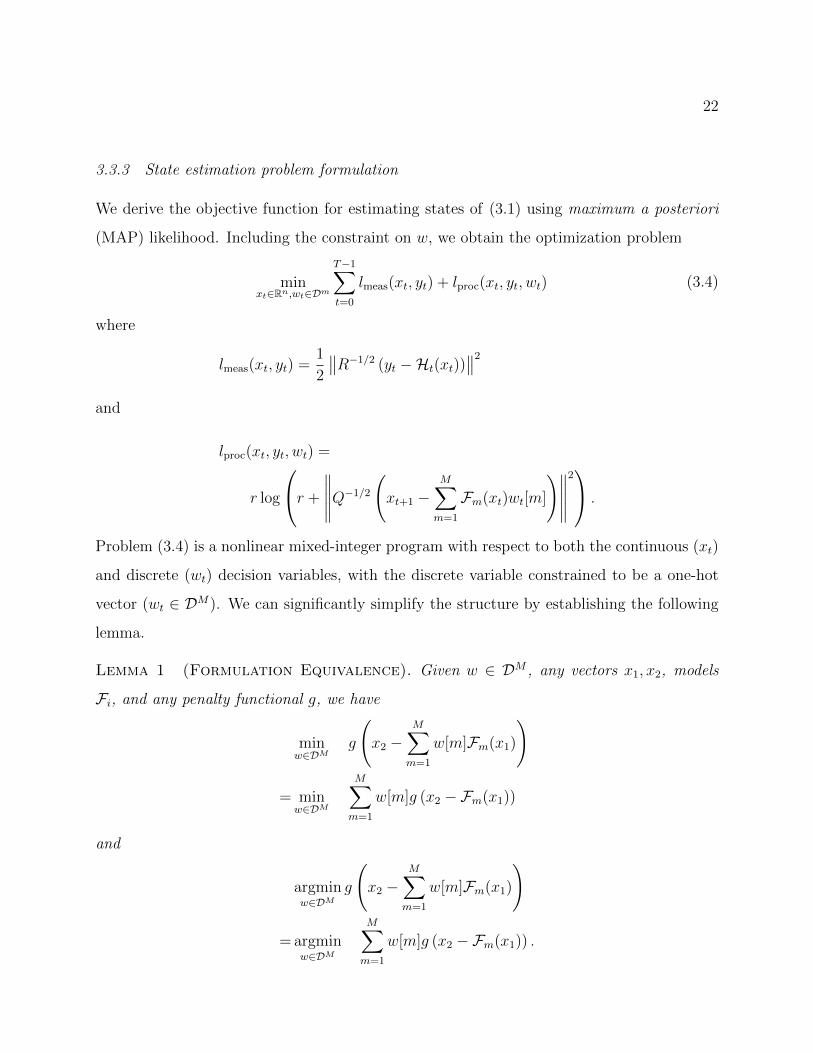
3.3.3 State estimation problem formulation

We derive the objective function for estimating states of (3.1) using maximum a posteriori

(MAP) likelihood. Including the constraint on w, we obtain the optimization problem

minxt∈Rn,wt∈Dm

T−1∑t=0

lmeas(xt, yt) + lproc(xt, yt, wt) (3.4)

where

lmeas(xt, yt) =1

2

∥∥R−1/2 (yt −Ht(xt))∥∥2

and

lproc(xt, yt, wt) =

r log

r +

∥∥∥∥∥Q−1/2

(xt+1 −

M∑m=1

Fm(xt)wt[m]

)∥∥∥∥∥2 .

Problem (3.4) is a nonlinear mixed-integer program with respect to both the continuous (xt)

and discrete (wt) decision variables, with the discrete variable constrained to be a one-hot

vector (wt ∈ DM). We can significantly simplify the structure by establishing the following

lemma.

Lemma 1 (Formulation Equivalence). Given w ∈ DM , any vectors x1, x2, models

Fi, and any penalty functional g, we have

minw∈DM

g

(x2 −

M∑m=1

w[m]Fm(x1)

)

= minw∈DM

M∑m=1

w[m]g (x2 −Fm(x1))

and

argminw∈DM

g

(x2 −

M∑m=1

w[m]Fm(x1)

)

= argminw∈DM

M∑m=1

w[m]g (x2 −Fm(x1)) .

23

Proof:

Since w ∈ DM for both problems, there are only M possible values for both objective

functions, i.e.

g(x2 −F1(x1)), g(x2 −F2(x1)), . . . , g(x2 −FM(x1)).

Hence, the minimum objective value for both problems will be minm g(x2 − Fm(x1)) and

every minimizer is a one-hot vector that selects a minimum value.

Based on Lemma 1, an equivalent formulation to (3.4) is given by

minxt∈Rn,wt∈DM

T−1∑t=0

(1

2

∥∥R−1/2 (yt −Ht(xt))∥∥2

+

M∑m=1

wt[m]r log(r +

∥∥Q−1/2 (xt+1 −Fm(xt))∥∥2))

.

(3.5)

Although still a mixed-integer program, this reformulation exhibits linear coupling between

the discrete variables wt and continuous variables xt. We will leverage this linear coupling

when we develop our estimation algorithm based on the relaxed problem formulation intro-

duced in the next section.

3.3.4 Relaxed state estimation problem formulation

Ultimately, the discrete state estimate will be specified as a one-hot vector, wt ∈ DM ⊂

RM . To formulate a continuous optimization problem that approximates the mixed-integer

problem formulated in the previous section, we relax the decision variable wt to take values in

the convex hull ∆M of DM .We use ∆M := w ∈ [0, 1]M : 1Tw = 1 to denote the simplex in

RM . The optimal relaxed wt will generally lie on the interior of the simplex, so we project the

result from our relaxed optimization problem to return the one-hot discrete state estimate.

Since this relaxation-optimization-projection process tends to induce frequent changes in the

discrete state estimate, we introduce a smoothing term on wt,

ν‖wt+1 − wt‖22,

24

yielding the continuous relaxation of (3.5) given by

minxt∈Rn,wt∈∆M

f(x,w) :=T−1∑t=0

(1

2

∥∥R−1/2 (yt −Ht(xt))∥∥2

+M∑m=1

wt[m]r log(r +

∥∥Q−1/2 (xt+1 −Fm(xt))∥∥2)

+ ν‖wt+1 − wt‖22

),

(3.6)

where x is the concatenated variable containing all xt, w is the concatenated variable con-

taining all wt, and ν is a parameter controlling the strength of smoothing. The optimal

relaxed discrete state estimate wt ∈ ∆M is projected onto DM by choosing the (unique)

one-hot vector whose argmaxmwt[m] component is equal to 1.

3.4 State estimation algorithm

In this section, we derive an algorithm to solve the relaxed state estimation problem formu-

lated in (3.6) using two key ideas:

1. nonsmooth variable projection;

2. Gauss-Newton descent with Student’s t penalties.

These two ideas are explained in the next two subsections, followed by a convergence

analysis in the third subsection.

3.4.1 Nonsmooth variable projection

The first idea is to pass to the value function, projecting out (partially minimizing over) the

w variables, so as to reduce the number of variables to optimize over. Define

v(x) := minwf(x,w) (3.7)

25

with f(x,w) as in (3.6). The objective f(x,w) is convex in w, but not strictly convex. To

guarantee differentiability of v(x), we add a smoothing term and consider

vβ(x) := minwf(x,w) +

β

2‖w‖2. (3.8)

where β is usually taken to be a very small number (e.g. 10−4 or smaller) so that the added

term has minimal effect on the original value function. (The minimizer of vβ is different from

that of v.) The function vβ(x) is a Moreau envelope [93, Def 1.22] of the true value function v;

we refer the interested reader to [7] for details and examples concerning the Moreau envelope

specifically (and nonsmooth variable projection more broadly). The unique minimizer w(x)

can be found quickly and accurately since the minimization problem with respect to w is

strongly convex: projected gradient descent converges linearly and can be accelerated using

the Fast Iterative Shrinkage-Thresholding Algorithm (FISTA) [15]. With the minimizer

w(x), the gradient of vβ is readily computed as

∇vβ(x) = ∂xf(x,w)|w=w(x). (3.9)

Plugging w(x) back into (3.6) we obtain the problem

minxvβ(x) =

1

2

T−1∑t=0

‖yt −H(xt)‖2R−1+ν‖wt+1(x)− wt(x)‖2

2

+M∑m=1

wt,m(x)r log

(1 +‖xt+1 −Fm(xt)‖2

Q−1

r

)+β

2‖w(x)‖2,

(3.10)

where wt,m(x) ≡ wt[m](x).

3.4.2 Gauss-Newton descent with Student’s t penalties

We derive a Gauss-Newton descent algorithm to solve (3.10) based on a line search method

first proposed in [27] for convex composite problems. To apply the method we first cast the

objective in (3.10) into a convex composite function, let vβ = ρ F , where

F (x) =

f1(x)

f2(x)

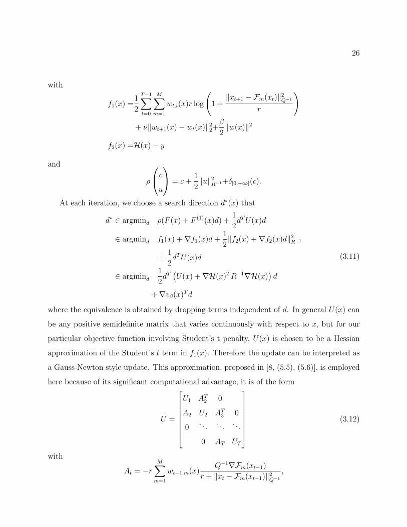
26

with

f1(x) =1

2

T−1∑t=0

M∑m=1

wt,i(x)r log

(1 +‖xt+1 −Fm(xt)‖2

Q−1

r

)+ ν‖wt+1(x)− wt(x)‖2

2+β

2‖w(x)‖2

f2(x) =H(x)− y

and

ρ

cu

= c+1

2‖u‖2

R−1+δ[0,+∞](c).

At each iteration, we choose a search direction d∗(x) that

d∗ ∈ argmind ρ(F (x) + F (1)(x)d) +1

2dTU(x)d

∈ argmind f1(x) +∇f1(x)d+1

2‖f2(x) +∇f2(x)d‖2

R−1

+1

2dTU(x)d

∈ argmind1

2dT(U(x) +∇H(x)TR−1∇H(x)

)d

+∇vβ(x)Td

(3.11)

where the equivalence is obtained by dropping terms independent of d. In general U(x) can

be any positive semidefinite matrix that varies continuously with respect to x, but for our

particular objective function involving Student’s t penalty, U(x) is chosen to be a Hessian

approximation of the Student’s t term in f1(x). Therefore the update can be interpreted as

a Gauss-Newton style update. This approximation, proposed in [8, (5.5), (5.6)], is employed

here because of its significant computational advantage; it is of the form

U =

U1 AT2 0

A2 U2 AT3 0

0. . . . . . . . .

0 AT UT

(3.12)

with

At = −rM∑m=1

wt−1,m(x)Q−1∇Fm(xt−1)

r + ‖xt −Fm(xt−1)‖2Q−1

,

27

Ut =rM∑m=1

wt,m(x)∇Fm(xt)TQ−1∇Fm(xt)

r + ‖xt+1 −Fm(xt)‖2Q−1

+wt−1,m(x)Q−1

r + ‖xt −Fm(xt−1)‖2Q−1

for 1 ≤ t ≤ T − 1, and

UT =rwT−1,m(x)Q−1

r + ‖xT −Fm(xT−1)‖2Q−1

.

We can rewrite U(x) as

U(x) =∑m

Fm(x)T Qm(w(x))−1Fm(x),

where

Gm(x) =

I 0 0

−∇Fm(x2) I 0 0

0. . . . . . . . .

. . . 0−∇Fm(xT ) I

and

Qm(w(x))−1 = diag(Qm,t(w(x))−1)

Qm,t(w(x))−1 =rwt−1,m(x)Q−1

r + ‖xt −Fi(xt−1)‖2Q−1

.

Clearly U(x) is positive semidefinite; we show in Lemma 3 that U(x) is actually positive

definite, so problem (3.11) reduces to the block tridiagonal linear system(U(x) +∇H(x)TR−1∇H(x)

)d+∇vβ(x) = 0.

Given d∗(x), the new x+ is of the form

x+ = x+ δd∗,

where δ is a step size selected using the Armijo-type [79, Sec. 3.1] line search criterion.

δ = maxγl:ρ(F (x+ γld∗)) ≤ ρ(F (x)) + cγl∆(x; d∗)

and c ∈ (0, 1)(3.13)

28

with

∆(x; d) = ρ(F (x) + F (1)(x)d) +1

2dTU(x)d− ρ(F (x)).

When d = 0, we have ∆(x; 0) = 04, and since we choose the minimizing

d∗ = argmind

ρ(F (x) + F (1)(x)d) +1

2dTU(x)d,

we have ∆(x; d∗) ≤ 0. Further,

∆(x; d∗) = 0⇔ 0 ∈ argmind

ρ(F (x) + F (1)(x)d) +1

2dTU(x)d

⇔ 0 ∈ ∂ρ(F (x))F (1)(x)

by [27, Thm. 3.6]. In other words, stationarity is achieved when ∆(x; d∗) = 0. When

∆(x; d) < 0, we are guaranteed to have descent

ρ(F (x) + F (1)(x)d) < ρ(F (x))

since U(x) is positive semidefinite. This condition ensures that the line search step (3.13) is

well-defined [27, Lemma 2.3].

Our approach is summarized in Algorithm 1. The positive parameter ε in the algorithm

specifies the stopping condition. Finally, we project the relaxed discrete state estimate

wt ∈ ∆M to obtain a discrete state estimate in DM as described in Section 3.3.4.

3.4.3 Convergence of state estimation algorithm

In this section we show the convergence of the proposed algorithm. The convergence of

Algorithm 1 to a stationary point for a general class of convex composite objective functions

is established in [27] and [8]. In particular [8, Theorem 5.1] establishes the possible outcomes

when applying this type of algorithm; informally, either the algorithm converges or the search

direction dk diverges. In the remainder of this section we provide two technical results needed

to formalize this intuition and to apply the aforementioned theorem:

4We overload ∆ here to match the notation in [8, 27]; ∆(x; d∗) should not be confused with ∆M , whichis used to denote the simplex containing relaxed state estimates.

29

Algorithm 1 Variable Projection for (3.6).

Require: x,w,Q,R, r, ν, β, ε

1: for k = 1, 2, 3, ... do

2: d(k) ← Gauss-Newton direction for x(k)

3: x(k+1) ← x(k) + δd(k)

4: w(k+1) ← InnerSolverΠt∆(w(k))

5: lossk ← f(x(k+1), w(k+1))

6:Iterate till ∆(x(k); d(k)) ≥ −ε.

• Lemma 2 establishes a set of sufficient conditions that prevent divergence (‖d(k)‖→ ∞);

• Lemma 3 proves that the sufficient conditions are satisfied.

Lemma 2. Let Λ = y|ρ(y) ≤ vβ(x(0)). If F−1(Λ) = x|F (x) ∈ Λ is bounded and U(x)

is positive definite for all x ∈ F−1(Λ), then the hypotheses in [8, Theorem 5.1] are satisfied

and the sequence of search directions d(k) is bounded.

Proof: The hypotheses in [8, Theorem 5.1] require that F (1) to be bounded and uni-

formly continuous on the set S = co(F (−1)(Λ)) where co stands for the closed convex hull.

F (1) is continuous on S since f(1)1 exists and is continuous by property of Moreau envelope

and proximal operator, and f(1)2 is continuous trivially. Further, given that S is closed by

definition and bounded by assumption, it is compact. Hence F (1) is bounded and uniformly

continuous on S.

Now we need to show that the sequence of search direction is bounded. At any iteration,

the search direction d we choose satisfies

0 ≤ ρ(F (x) + F (1)(x)d) +1

2dTU(x)d ≤ ρ(F (x)) ≤ ρ(F (x0))

where the first inequality relies on ρ ≥ 0 and on the positive semidefinite property of U(x);

the second inequality comes from ∆(x; d) ≤ 0; the third inequality results from the line

search condition that creates a decreasing sequence ρ(F (x(k)).

30

Since ρ(F (x0)) is finite, dTU(x)d <∞ for all iterations. Because Λ is closed by closedness

of ρ and F is continuous, F−1(Λ) is also closed. Along with its boundedness by assumption,

F−1(Λ) is compact. Since x ∈ F−1(Λ) 7→ λmin(U(x)) is continuous, its image is bounded,

hence given that U(x) is positive definite there exists some λmin > 0 for all x ∈ F−1(Λ).

Therefore 0 < λmin‖d‖2≤ dTU(x)d <∞, which implies that d(k) cannot be unbounded.

Lemma 3. F−1(Λ) is bounded for problem (3.10) and U(x) is positive definite for all x ∈

F−1(Λ).

Proof: First note that Λ is bounded by the coercivity of ρ. This implies that for an

unbounded sequence ‖x(k)‖→ ∞, we still have f1(x(k)) <∞ and ‖f2(x(k))‖<∞.

If ‖x(k)‖→ ∞, then we can find some t+ 1 and a subsequence J such that limk∈J‖x(k)t+1‖=

∞. By the definition of f1 and f1(x(k)) < ∞, limk∈J‖Fi(x(k)t )‖= ∞, which further implies

that limk∈J‖x(k)t ‖= ∞. Iteratively this means that limk∈J‖x(k)

t ‖= ∞ for all t, in particular

for the given starting point x0, but that is not possible.

To show that U(x) in (3.12) is positive definite, recall that we can rewrite U(x) as

U(x) =∑m

Gm(x)T Qm(w(x))−1Gm(x) 0.

If there exists some d such that dTU(x)d = 0, then

dT

(∑m

Gm(x)T Qm(w(x))−1Gm(x)

)d

=∑m

dTGm(x)T︸ ︷︷ ︸zm(x)T

Qm(w(x))−1Gm(x)d︸ ︷︷ ︸zm(x)

=∑m

zm(x)T Qm(w(x))−1zm(x) = 0,

⇒zm(x)T Qm(w(x))−1zm(x) = 0 ∀i

⇒zm,t(x)T Qm,t(w(x))−1zm,t(x) = 0∀t ∀i

since Qm(w(x))−1 = diag(Qm,t(w(x))−1), and

Qm,t(w(x))−1 =rw(x)t,mQ

−1

r + ‖xt+1 −Fm(xt)‖2Q−1

31

are positive semidefinite. However because each wt ∈ ∆, there has to be some Q−1m,t 0 for

each t. Therefore U(x) must be positive definite for all x ∈ F−1(Λ).

3.5 Parameter Tuning for Proposed Algorithm

Before we present numerical results, we include a general guidance on parameter tuning for

the new algorithm. We discuss both standard parameters (e.g. Q, R) that must be tuned

by any algorithm for this application, as well as the parameters ν and r which are specific to

our approach. We first give a rough outline of steps we have taken to tune the parameters,

followed by more detailed guidelines to tune each individual parameter.

1. Start with large r for Student’s t, i.e. distribution close to Gaussian.

2. If Q and R are unknown, they are tuned such that the smooth part of trajectories can

be well approximated.

3. Decrease degrees of freedom r of Student’s t so that the nonsmooth part of trajectories

can be captured.

4. Adjust smoothing coefficient ν to reduce number of switches.

For degrees of freedom r, one can start with a large value, meaning that the distribution is

close to Gaussian, and decrease it later to capture jumps in the continuous state.

For covariance matrices Q and R, if empirical estimations are available, they can be

supplied to the model directly. There is existing literature on estimation methods for noise

covariance matrices [30]. When such estimations are not available, we usually assume the

matrices to be diagonal for simplicity, in which case the inverse of diagonal entries can also

be interpreted as weights. The diagonal values of R represent variance for measurements.

When choosing R, we consider the relative scale of measurements, e.g. measurements with

smaller magnitude usually have smaller variance. For choices of diagonal values of Q, we

32

usually assign smaller variance for observed states, e.g. positions in our examples,and larger

variance for unobserved states.

The choice of smoothing coefficient ν depends on modeler’s belief in frequency of switches.

One can start with a small value of ν (i.e. little penalty on frequent switches), and gradually

increase it, till the pattern of switches is close to modeler’s belief.

We recommend having a short piece of manually labeled trajectories as a training set for

the purpose of parameter tuning. After tuning, the user can apply the same parameters on

larger dataset collected from similar scenarios.

In terms of sensitivity of estimation results on parameters, we had the following observa-

tions when running our experiments:

• The estimation result is not very sensitive to r. We were able to decrease r fairly

aggressively during parameter tuning.

• For the diagonals of Q and R, we found that it was important to have values in the

correct ranges, but the exact values taken were not crucial.

• For smoothing coefficient ν, we noticed that the switching times were sensitive to ν

when ν was very small relative to the diagonal entries of Q−1 and R−1. Since we

assumed that the discrete states should not change too frequently, we used a slightly

larger ν.

3.6 Comparison with the Interacting Multiple Model (IMM) method

We compare the nonsmooth variable projection algorithm5 (Algorithm 1) with the Interacting

Multiple Model (IMM) [19] algorithm implemented in the open-source package filterpy [58].

We consider two examples, in both cases the continuous state x is a scalar, and there are

two discrete states. In the first example, the continuous state x undergoes no jumps, i.e. the

5We provide an implementation of Algorithm 1 and the comparison results in this section at https:

//github.com/jizezhang/hds-state-estimation (and duplicated at https://github.com/apace2/

hds-state-estimation).

33

reset is the identity function. In the second example, the continuous state x undergoes an

instantaneous jump when the discrete state changes; i.e. a non–identity reset. The dynamics

of the two discrete state process models are:

x = −1 Fw=1,

x = 1 Fw=2.

For the second example with non–identity resets, when a discrete state switch occurs, the

continuous state decreases by 5. In both examples the discrete state switches at t = 1 and

t = 2. Additionally, the measurement noise has a variance of R = [.0001], which is used

as the measurement noise covariance for all models. IMM1 uses a process noise model of

covariance Q = [.001] for both the internal Kalman filters and IMM2 uses a process normal

process noise model with covariance Q = [.2].

In the first example, Algorithm 1 (VP) and IMM perform nearly identically (Figure 3.2).

Both methods accurately recover the continuous state and discrete state. When the system

undergoes instantaneous jumps in the continuous state at discrete state changes, Algorithm 1

outperforms IMM (Figure 3.3). For IMM, there is a clear trade–off exists between recovering

the continuous state and recovering the discrete state. When using a process noise model

with large covariance, as in the case of IMM2, the continuous state can be recovered at the

expense of the discrete state. In the top subplot of Figure 3.3, wIMM2 is nearly the same

value for the duration of the simulation, with slight separation between the two modes. With

a smaller covariance, as in IMM1, the discrete state can be recovered. From t = 1 to near

t = 1.25, IMM1 incorrectly identifies the discrete state due to the continuous state jump

direction being opposite of the continuous state dynamics for discrete state w = 2.

Both Algorithm 1 and IMM require a similar number of parameters from the user. For

both methods, covariance matrices for the process error model Q and measurement error

model R need to be provided. IMM adjusts the estimated frequency of switching between

the discrete states via a probability transition matrix while Algorithm 1 uses the smoothing

parameter ν, Sec. 3.3.4. Algorithm 1 has one additional parameter r due to the process noise

34

Time (s)

x

x = 1 x = −1

Figure 3.2: Algorithm 1 (VP) performs comparably to IMM when the continuousstate does not undergo any resets. The top plot shows the true state w and the simplexestimate of the true state from both methods wV P , wIMM1 . The simplex estimate is shownin color and the probability estimate of the discrete state being w = 1 is superimposed as ablack line. The middle plot shows the actual value of the continuous state of the simulationand the estimates. The bottom plot shows the residual between true continuous state andthe estimated continuous state.

Time (s)

x

x = 1 x = −1

Figure 3.3: Algorithm 1 (VP) outperforms the IMM when there are jumps in thecontinuous state. The plots follow the convention laid out in Figure 3.2.

35

model being Student’s t distribution, which is crucial for obtaining accurate estimates with

non–identity resets, Sec. 3.3.2.

3.7 Experiments with hybrid system models

To evaluate the proposed approach to state estimation for hybrid systems, we apply our

algorithm to linear and nonlinear impact oscillators. In addition to being well-studied (

[28, §1.2], [95]), these mechanical systems were chosen since they are among the simplest

physically-relevant models that have non–identity reset maps. The parameter and trajec-

tory regime considered in what follows is representative of a jumping robot constructed from

one limb of a commercially-available quadrupedal robot [52] and controlled with an event-

triggered stiffness adjustment; Figure 3.4a contains a photograph of the limb. The jump-

ing robot’s hip and foot are constrained to move vertically in a gravitational field, so the

rigid pantograph mechanism depicted in Figure 3.4b has two mechanical degrees-of-freedom

(DOF) coupled through nonlinear pin-joint constraints. These two DOF are preserved, but

their nonlinear coupling is neglected, in the piecewise-linear model illustrated in Figure 3.4c.

The hybrid dynamics of these linear and nonlinear impact oscillators are specified in Sec-

tion 3.7.1

We perform two sets of experiments. The first set of experiments in Sec. 3.7.2 concern the

piecewise-linear model depicted in Figure 3.4c and explore the consequences of our modeling

assumptions and the efficacy of our proposed algorithm:

• Sec. 3.7.2 demonstrates the advantage of employing a Student’s t distribution for pro-

cess noise as compared to a Gaussian distribution;

• Sec. 3.7.2 demonstrates the superior convergence rate yielded by Gauss-Newton descent

directions as compared to gradient (steepest) descent;

• Sec. 3.7.2 demonstrates the advantage of smoothing the relaxed discrete state estimate;

and

36

(a)

q[1]

q[2] g

(b)

k1, k2

q[1]

q[2] g

(c)

Figure 3.4: Jumping robot and impact oscillator hybrid system models (Sec. 3.7.1).(a) Photograph of the physical robot (one leg from a Minitaur [52]) that inspired the sim-ulation models. (b) Nonlinear model consisting of two masses coupled with a linear springand a nonlinear pantograph mechanism. (c) Linear model consisting of two masses coupledwith a linear spring.

• Sec. 3.7.2 demonstrates the algorithm’s performance when onboard measurements are

used instead of offboard measurements.

The second set of experiments in Sec. 3.7.3 evaluate our proposed approach using the non-

linear model depicted in Figure 3.4b.

Since this section is devoted to comparing estimated states to ground truth simulation re-

sults, and since our approach entails the determination of a relaxed discrete state estimate en

route to obtaining the discrete state estimate, we now introduce notation that distinguishes

these quantities:

• wt ∈ DM denotes the ground truth discrete state;

• wt ∈ ∆M denotes the relaxed discrete state estimate;

• wt ∈ DM denotes the discrete state estimate.

This notational distinction was not introduced previously in the interest of readability since

there was no ambiguity entailed by overloading notation in the problem formulation and

algorithm specification.

37

3.7.1 Impact oscillator hybrid system models

The continuous state x = (q, q) ∈ R4 for the jumping robot hybrid system model consists of

the two-dimensional configuration vector q ∈ R2 and corresponding velocity q ∈ R2, where

q[1] and q[2] denote the vertical height of the hip and foot, respectively. The foot is not

permitted to penetrate the ground, q[2] ≥ 0, so the first part of the discrete state indicates

whether this constraint is active: A (air) if q[2] > 0, G (ground) if q[2] = 0. To compensate

for energy losses at impact, an event-triggered controller stiffens or softens a spring based

on which direction the hip is traveling, so the second part of the discrete state indicates the

direction of travel for q[1]: ↑ if up, ↓ if down. With qm(q, q) ∈ R2 denoting the acceleration

of the hip and foot in discrete state m ∈ A↓,G↓,G↑,A↑,6 formula for this acceleration

are given in Table 3.1. At the moment of impact (when the discrete state changes from

wt ∈ A ↓,A ↑ to wt+1 ∈ G ↓,G ↑) the foot velocity q[2] is instantaneously reset to 0,

corresponding to perfectly plastic impact. An example of the jump in continuous state when

transitioning from A↓ to G↓ on the foot velocity q[2] is shown in Figure 3.5 near time 17.5s.

3.7.2 Piecewise-linear impact oscillator experiment

In this subsection, we employ the linear spring laws

k1(q, q) = 10(q[1]− q[2])− 3,

and

k2(q, q) = 15(q[1]− q[2])− 3,

with parameter values mh = 3,mt = 1, g = 2. Appendix A.2 contains a complete definition

of the hybrid system.

In our first demonstration the observed states are q[1] and q[2], position of the hip and

foot, leaving the velocities unobserved:

Hpos(x) = q. (3.14)

6To simplify exposition we identify m = A ↓ with m = 1, m = G ↓ with m = 2, m = G ↑ with m = 3,and m = A↑ with m = 4.

38

Discrete state w Icon qw(x)

w = A↓[ 1mh

(−k1(q, q))− g1mt

(k1(q, q))− g

]

w = G↓[

1mh

(−k1(q, q))− g0

]

w = G↑[

1mh

(−k2(q, q))− g0

]

w = A↑[ 1mh

(−k2(q, q))− g1mt

(k2(q, q))− g

]

Table 3.1: Discrete states and continuous dynamics for impact oscillator hybridsystem models (Sec. 3.7.1). Note that the continuous dynamics q have the same generalform for both the piecewise-linear and -nonlinear models, with the spring law k being alinear or nonlinear function of the continuous state x = (q, q) depending on which model isconsidered.

State estimation results for this system are shown in Figure 3.7b.

In the remainder of this subsection, we demonstrate the effects of the choices we made in

our problem formulation (Sec. 3.3) and algorithm derivation (Sec. 3.4) using the piecewise-

linear model as a running example. We also consider a variation where the measurements

correspond to the leg length and velocity, which are more representative of the onboard

measurements available to an autonomous robot operating outside of the laboratory.

Student’s t versus Gaussian process noise

Figure 3.5 compares the estimation of foot velocity using Student’s t with r = 0.01 versus

using Gaussian for the process noise distribution; in both cases the true discrete state is given.

The estimated trajectory for both distributions match the true simulated trajectory away

from jumps, while near jumps, such as around times 16.6s and 17.5s, using the Student’s t

distribution enables closer tracking of the instantaneous change in the true foot velocity q[2]

39

16.0 16.5 17.0 17.5 18.0

Time (s)

−4

−2

0

Foot

Vel

oci

tyq[

2](m

/s)

Student’s t Process Noise

Gaussian Process Noise

Simulation

Figure 3.5: The Student’s t distribution process noise yields better estimates ofinstantaneous changes in continuous state (Sec. 3.7.2). In this plot, estimates of thefoot velocity are shown near two impacts (≈ 16.6s, 17.5s).

than when using a Gaussian distribution.

Gauss-Newton versus gradient (steepest) descent

We empirically compared convergence rates for continuous state xt updates obtained using

Gauss-Newton and gradient (steepest) descent directions (Algorithm 1, line 2). Figure 3.6

shows the log loss versus algorithm iteration for the two methods; the actual discrete state wt

was taken as given to perform this comparison. As expected, the objective value decreases

significantly faster when the search direction is determined by the Gauss-Newton scheme as

compared to the direction of steepest descent, reaching the stopping criterion in ten times

fewer iterations in our tests.

Smoothing the relaxed discrete state versus not

If the continuous states are given, the discrete state estimate returned by our algorithm

(skipping lines 2 and 3 of Algorithm 1) is very close to the true discrete state regardless

of whether a smoothing term is included in the relaxed problem formulation. When simul-

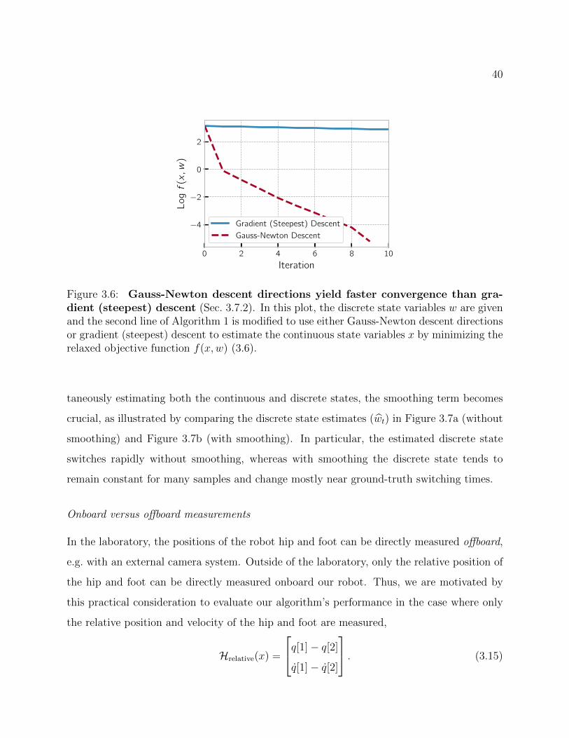
40

0 2 4 6 8 10

Iteration

−4

−2

0

2

Lo

gf

(x,w

)

Gradient (Steepest) Descent

Gauss-Newton Descent

Figure 3.6: Gauss-Newton descent directions yield faster convergence than gra-dient (steepest) descent (Sec. 3.7.2). In this plot, the discrete state variables w are givenand the second line of Algorithm 1 is modified to use either Gauss-Newton descent directionsor gradient (steepest) descent to estimate the continuous state variables x by minimizing therelaxed objective function f(x,w) (3.6).

taneously estimating both the continuous and discrete states, the smoothing term becomes

crucial, as illustrated by comparing the discrete state estimates (wt) in Figure 3.7a (without

smoothing) and Figure 3.7b (with smoothing). In particular, the estimated discrete state

switches rapidly without smoothing, whereas with smoothing the discrete state tends to

remain constant for many samples and change mostly near ground-truth switching times.

Onboard versus offboard measurements

In the laboratory, the positions of the robot hip and foot can be directly measured offboard,

e.g. with an external camera system. Outside of the laboratory, only the relative position of

the hip and foot can be directly measured onboard our robot. Thus, we are motivated by

this practical consideration to evaluate our algorithm’s performance in the case where only

the relative position and velocity of the hip and foot are measured,

Hrelative(x) =

q[1]− q[2]

q[1]− q[2]

. (3.15)

41

Time (s)

q[2] velocity (m/s)

q[1] velocity (m/s)

q[1], q[2] position (m)

A↓ G↓ G↑ A↑

(a) Without Smoothing (ν = 0)

Time (s)

q[2] velocity (m/s)

q[1] velocity (m/s)

q[1], q[2] position (m)

A↓ G↓ G↑ A↑

(b) With switching (ν > 0)

Figure 3.7: Without smoothing (ν = 0), the discrete state estimate switches fre-quently (Sec. 3.7.2). With smoothing (ν > 0), the discrete state estimate mostlyswitches near the true switching times. (Sec. 3.7.2). The top plot shows the truediscrete state of the system w ∈ DM , the relaxed discrete state estimate w ∈ ∆M , andthe discrete state estimate w ∈ DM for a simulation of the piecewise-linear system. Thesubsequent plots show the estimate, simulation, and error ε values for position and velocityof the hip q[1] and foot q[2].

42

Time (s)

A↓ G↓ G↑ A↑

Figure 3.8: Estimated discrete state using onboard (relative position and velocity)measurements Hrelative (3.15) for the piecewise-linear system closely matches truediscrete state. (Sec. 3.7.2). Continuous state estimates are not shown since they areformally unobservable using only onboard measurements (in practice, they drift away fromground truth over time).

Although the full hybrid system state is formally unobservable with these relative mea-

surements, our algorithm nevertheless yields good estimates of the discrete state as shown

in Figure 3.8; due to large errors in the estimate of (unobservable) continuous states, we

omit those results from the figure.

3.7.3 Piecewise-nonlinear impact oscillator experiment

To test Algorithm 1 on a nonlinear model, we included the kinematic constraints depicted in

Figure 3.4b, resulting in a nonlinear spring force. In this model we set the two spring laws

to be the same k1 = k2, decreasing the number of discrete states from four to two: w = A

when q[2] > 0 and w = G when q[2] = 0. Appendix A.3 contains the complete hybrid system

description for the model. State estimation results compare favorably with the analogous

results from the piecewise-linear system when using either absolute position measurements

Hpos (3.14) (compare Figure 3.9a with Figure 3.7b) or relative measurements Hrelative (3.15)

(compare Figure 3.9b with Figure 3.8).

In Figure 3.9a we see that the model can estimate continuous and discrete states in the

nonlinear setting. However, we do notice that the estimated trajectories are not as close to

ground truth as in the linear case. In particular, when q[2] has a value only slightly greater

than 0 (e.g. between times 3s and 4s), the algorithm fails to detect the transition between

43

w = A and w = G.

3.8 Conclusion

We proposed a new state estimation algorithm for hybrid systems, analyzed its convergence

properties, compared with IMM, and evaluated its performance on piecewise-linear and -

nonlinear hybrid systems with non–identity resets. The algorithm leverages a relaxed state

estimation problem formulation where the decision variables corresponding to the discrete

state are allowed to take on continuous values. This relaxation yields a continuous optimiza-

tion problem that can be solved using recently-developed nonsmooth variable projection

techniques. The effectiveness of the approach was demonstrated on hybrid system models of

mechanical systems undergoing impact.

44

Time (s)

q[2] velocity (m/s)

q[1] velocity (m/s)

q[1], q[2] position (m)

A G

(a) Continuous and discrete states estimated for the piecewise-nonlinear model(Sec. 3.7.3). Notational and plotting conventions are adopted from Figure 3.7.

Time (s)

GA

(b) Estimated discrete state using onboard (relative position and velocity) measure-ments Hrelative (3.15) for the piecewise-nonlinear system closely matches true discretestate. (Sec. 3.7.2). As with Figure 3.8, continuous state estimates are not shown since they driftfrom the true values over time.

Figure 3.9: State estimatotion for a piecewise-nonlinear model (Sec. 3.7.1); note the nonlinearmodel only has two discrete states.

45

Chapter 4

PIECEWISE–DIFFERENTIABLE FLOW1

4.1 Abstract

The goal of this paper is to present the conditions under which a mechanical system with

unilateral constraints is PCr and under which it is at least once C1. Additionally we provide

an example of such systems.

4.2 Introduction

In this paper we handle rigid mechanical systems subject to unilateral constraints, a type

of mechanism with many applications including locomotion and manipulation. One key

characteristic of such system is the discontinuous trajectories that result from impact with

unilateral constraints. While the trajectories themselves are discontinuous, under certain

circumstances away from points of impact, the flow is differentiable. Ignoring grazing, it is

well known that the flow is classically differentiable near trajectories undergoing indepen-

dent contacts [2]. The same is not the case near trajectories with simultaneous impacts, one

example is the flow for a rocking block [67] which is discontinuous along such trajectories.

When unilateral constraints are orthogonal with respect to the mass inverse matrix the flow

is at least continuous even for simultaneous impacts [10]. In this work we show that along

admissible trajectories the flow is piecewise–differentiable, a class of differentiability stronger

then directional differentiable and weaker than classical differentiable. We use the notion of

piecewise–differentiable from [91,96], which provides similar properties as classically differen-

tiable, e.g. composition, chain rule, and implicit function theorem [96, Chp. 3] We next show

with even greater restriction to the system, of which limbs decoupled through the body is a

1Portions of this chapter originally appeared in [83,84]

46

subset of [83], the flow is classically differentiable along trajectories even with simultaneous

impacts.

Much work has gone into characterizing flows for systems with switching vector fields. [2]

The work in [2] shows the existence of a first-order approximation for a continuous trajectory

undergoing a discontinuous change in the underlying vector field when all nearby trajectories

undergo the same sequence of vector field changes; [2, (2.5)] is the well known saltation (or

jump update) matrix. This result is extended to continuous left-hand side trajectories in

[49].2 [23] generalizes the result of [2] to cases where nearby trajectories may undergo differing

switching orders and shows the flow to be piecewise–differentiable. Similar result are shown

in [90, 94], where sensitivity analysis is provided for fixed mode sequences and potentially

varying mode sequences respectively. All the above results come from hybrid dynamics. [57]

provides a differentiability result when the dynamics stem from a complementarity problem.

4.3 Background

Within this section we cover well known properties of mechanical systems interacting with

unilateral constraints. We utilize two common formalisms for modeling mechanical systems

undergoing impacts (i) measure differential equations / inclusion and (ii) hybrid dynamical

systems.3 Measure differential inclusion provides the key result of existence and uniqueness

[10, Thm. 10] and continuity [10, Thm. 20] of flow.4

The section is organized as follows, we first define constraints and what contact is and

provide a key assumption orthogonality of constraints. Next, we introduce the well known

dynamics of the system, and introduce assumptions to guarantee existence and uniqueness

of the flow followed by a reiteration of [10, Thm. 20]. Next we state key assumptions on

what makes a given trajectory admissible.

2In [49], the notion of piecewise–differentiable is introduced for trajectories undergoing up to two simul-taneous impacts but means directional derivative as opposed to the stronger notion provided by [91].

3Other modeling conventions are singular perturbations and complementarity systems [61, Chp. 1].

4To the best of the authors’ knowledge, there are no comparable results to [10, Thm. 20] using the hybriddynamical systems formalism for mechanical systems subject to unilateral impacts.

47

Figure 4.1: Figure of a basic example piecewise differentiable flow. The pictured system is

described in detail in section 4.5.1

48

4.3.1 Mechanical Systems Subject to Unilateral Constraints

In this paper, we study the dynamics of a mechanical system with configuration coordinates

q ∈ Q = Rd subject to n (perfect, holonomic, scleronomic)5 unilateral constraints

ai(q) ≥ 0, ∀i ∈ 1, 2, · · · , n, (4.1)

where ai:Q→ R is differentiable and n, d ∈ N. We are primarily interested in systems with

n > 1 constraints. Given any ordered set J ⊂ 1, . . . , n with the natural ordering, and

letting |J | denote the number of elements in J , we let aJ :Q → R|J | denote the function

defined by

(aJ)i (q) = aJi(q) (4.2)

for all i ∈ J and q ∈ Q, with a∅(q) = 0.

Definition 2 (contact modes). With A = q ∈ Q|ai(q) ≥ 0 ∀i ∈ 1, . . . , n denoting

the set of admissible configurations, the constraint functions ajnj=1 partition A into a finite

collection6 AJJ∈2n of contact modes:

∀J ∈ 2n : AJ = q ∈ Q | aJ(q) = 0,∀i 6∈ J : ai(q) > 0. (4.3)

We let TA = (q, q) ∈ TQ : q ∈ A and TAJ = (q, q) ∈ TQ : q ∈ AJ for each J ∈ 2n.

Definition 3 ((in)active constraints). For an admissible configuration q ∈ AJ ⊂ A,

we refer to the J as the set of active constraints and the set j ∈ 1, 2, . . . , n|aj(q) > 0 as

the set of inactive constraints.

Remark 10. In definition 2, J = 1, . . . , n indexes the maximally constrained contact

mode and J = ∅ indexes the unconstrained contact mode.

5A constraint is: perfect if it only generates force in the direction normal to the constraint surface;holonomic if it varies with configuration but not velocity; scleronomic if it does not vary with time. Wewill discuss the inclusion of imperfect, nonholonomic, or nonscleronomic constraints in section 4.6.

6We let 2n = J ⊂ 1, . . . , n denote the power set (i.e. the set containing all subsets) of 1, . . . , n.

49

Assumption 1 (independent constraints [10, §3.4]). The constraints are indepen-

dent:

∀J ∈ 2n, q ∈ a−1J (0) : Daj(q)j∈J ⊂ T ∗qQ is linearly independent. (4.4)

Remark 11. Algebraically, Assumption 1 (independent constraints) implies that the con-

straint forces λJ are well–defined, and that there are no more constraints than degrees–of–

freedom, n ≤ d. Geometrically, it implies for each J ∈ 2n that a−1J (0) ⊂ Q is an embedded

codimension–|J | submanifold, and that the codimension–1 submanifoldsa−1j (0)

j∈J inter-

sect transversally; this follows from [59, Thm. 5.12] since (4.4) states that aJ :Q → R is

constant–rank on its zero section.

Assumption 2 (orthogonal constraints [10, Thm. 20]). Constraint surfaces in-

tersect orthogonally:

∀i, j ∈ 1, . . . , n , i 6= j, q ∈ a−1i (0) ∩ a−1

j (0) : 〈Dai(q), Daj(q)〉M−1 = 0. (4.5)

Remark 12. Note that Assumption 2 (orthogonal constraints) is strictly stronger than As-

sumption 1 (independent constraints). Physically, the assumption can be interpreted as as-

serting that any two independent limbs that can undergo impact simultaneously must be in-

ertially decoupled. This can be achieved in artifacts by introducing series compliance in a

sufficient number of degrees–of–freedom.

It is well–known (see e.g. [10, Sec. 3] or [50, Sec. 2.4, 2.5]) that for a constant contact mode

with J = j ∈ 1, . . . , n : aj(q) = 0, the set of active constraints, the system’s dynamics

take the form

M(q)q = f(q, q)− c(q, q)q +DaJ(q)>λJ(q, q), (4.6a)

q+ = ∆J(q, q−)q−, (4.6b)

where M :Q→ Rd×d specifies the mass matrix (or inertia tensor) for the mechanical system

in the q coordinates, f :TQ → Rd is termed the effort map [10] and specifies7 the internal

7We let TQ = Rd × Rd denote the tangent bundle of the configuration space Q; an element (q, q) ∈ TQcan be regarded as a pair containing a vector of generalized configurations q ∈ Rd and velocities q ∈ Rd;we write q ∈ TqQ.

50

and applied forces, c:TQ→ Rd×d denotes the Coriolis matrix determined8 by M , DaJ :Q→

R|J |×d denotes the (Jacobian) derivative of the constraint function aJ with respect to the

coordinates, λJ :TQ → R|J | denotes the reaction forces generated in contact mode J to

enforce the set of active unilateral constraints, aJ(q) = 0 [66, (4.5)],

λJ(q, q) = −ΛJ(q)

(Da(q)M−1(q) (f(q, q)− c(q, q)q) +

d

dt(DaJ)(q)q

), (4.7)

∆J :TQ → Rd×d specifies the collision restitution law that resets velocities to ensure com-

patibility with the active unilateral constraints, and q+ (resp. q−) denotes the right– (resp.

left–)handed limits of the velocity vector with respect to time.

Given Assumption 2 (orthogonal constraints), the impact law eq. (4.6b) has a unique

solution [50, Sec. 2.5]

∆(q, q) = Id − (1 + γ(q))M(q)−1DaJ(q)>ΛJ(q)DaJ(q),

where Id is the d–dimensional identity matrix, γ:Q → [0, 1] is a continuous function speci-

fying the coefficient of restitution,and ΛJ :Q→ Rd×d is given by

ΛJ(q) =(DaJ(q)M(q)−1DaJ(q)>

)−1,

and Λ∅(q) = 0

Remark 13. When only constraint deactivations occur, q+ = ∆J(q, q−)q− = q−. In a

similar vain, we adopt the convention ∆∅(q, q) = Id since any velocity is allowable in the

unconstrained mode.

Remark 14. Equation eq. (4.6) generates a right hand continuous flow, with discontinuities

whenever a constraint is activated. It is import to note eq. (4.6b) does not apply only when

the constraint mode changes, indeed at every instant in time eq. (4.6b) for a constant mode

J q+ = ∆J(q, q−)q− = q− as λJ ensures aJ(q) = 0.

8For each `,m ∈ 1, . . . , d the (`,m) entry c`m is determined from the entries of M via

c`m =1

2

d∑k=1

(DkM`m +DmM`k −D`Mkm) .

51

In the present paper, we will assume that appropriate conditions have been imposed to

ensure trajectories of eq. (4.6) exist on a region of interest in time and state.

Assumption 3 (existence and uniqueness [10, Thm. 10]). There exists a flow for eq. (4.6),

that is, a function φ : F → TA where F ⊂ [0,∞) × TA is an open subset containing

0 × TA and for each (t, (q, q)) ∈ F the restriction φ|[0,t]×(q,q): [0, t] → TQ is the unique

left–continuous trajectory for eq. (4.6) initialized at (q, q).

Remark 15. The problem of ensuring trajectories of eq. (4.6) exist and are unique has been

studied extensively; we refer the reader to [10, Thm. 10] for a specific result and [50] for a

general discussion of this problem.

Since we are concerned with differentiability properties of the flow, we assume the ele-

ments in eq. (4.6) are differentiable.

Assumption 4 (Cr vector field and reset map [10, §3.4]). The vector field eq. (4.6a)

and reset map eq. (4.6b) are continuously differentiable to order r ∈ N.

Remark 16. If we restricted our attention to the continuous–time dynamics in eq. (4.6),

then Assumption 4 would suffice to provide the local existence and uniqueness of trajectories

imposed by Assump. 3; as illustrated by [10, Ex. 2], Assumption 4 does not suffice when the

vector field eq. (4.6a) is coupled to the reset map eq. (4.6b).

Remark 17. The problem of ensuring trajectories of (4.6) exist and are unique has been

studied extensively; we refer the reader to [10, Thm. 10] for a specific result and [50] for a

general discussion of this problem.

4.3.2 Differentiability for constant contact mode sequence

It is possible to satisfy the hypothesis of Assumption 3 (existence and uniqueness of flow)

under mild conditions that allow trajectories to exhibit phenomena such as grazing (wherein

the trajectory activates a new constraint without undergoing impact) or Zeno (wherein the

52

(q0, q0)

q+ = ∆q−

(qt, qt)

a(q)

=0

Figure 4.2: Example of what a constant contact mode sequence means for differentiation

and why differentiable

trajectory undergoes an infinite number of impacts in a finite time interval). In this and

subsequent sections, where we seek to study differentiability properties of the flow, we will

not be able to accommodate grazing and Zeno phenomena. Therefore we proceed to restrict

the trajectories under consideration.

One import reminder is that while we seek criteria that denote differing concepts of dif-

ferentiability of the flow, this does not imply the flow is everywhere continuous. Importantly,

permissible trajectories with constraint activations must be discontinuous. Instead, the re-

strictions of considering trajectories will enforce continuity of final condition with respect to

perturbations of the initial condition. That is, under assumptions laid out in this section,

φ is a continuous function nearby (t, (q, dotq)), Fig. 4.2 provides an example of a classically

differentiable flow with a discontinuous trajectory.

Definition 4 (constraint activation/deactivation). The trajectory φ(q,q) initial-

ized at (q, q) ∈ TAJ ⊂ TQ activates constraints I ∈ 2n at time t > 09 if (i) no constraint

in I was active immediately before time t and (ii) all constraints in I become active at time t.

9We also informally refer to a constraint activating as impacting constraints I due to, once excludinggrazing trajectories, all constraint activations cause a discontinuity in the velocity according to eq. (4.6b).

53

Formally,10

∃ε > 0 : I ∩ J = ∅, (i) φ ((t− ε, t), (q, q)) ⊂ TAJ ,

(ii) φ(t, (q, q)) ∈ TAI∪J .(4.8)

We refer to t as a constraint activation time for φ(q,q). Similarly, the trajectory φ(q,q) deac-

tivates constraints I ∈ 2n at time t > 0 if (i) all constraints in I were active at time t and

(ii) no constraint in I remains active immediately after time t. Formally,

∃ε > 0 : I ⊂ J, (i) φ(t, (q, q)) ∈ TAJ ,

(ii) φ ((t, t+ ε), (q, q)) ⊂ TAJ\I .(4.9)

Definition 5 (Admissible (de)activation). A constraint activation time t > 0 for

φ(q,q) is admissible if the constraint velocity11 for all activated constraints I ∈ 2n is negative.

Formally, with (ρ, ρ−) = lims→t− φ(s, (q, q)) denoting the left–handed limit of the trajectory

at time t,

∀i ∈ I : Dt [ai φ] (0, (ρ, ρ−)) = Dai(ρ)ρ− < 0. (4.10)

for all activated constraints I ∈ 2d is negative.

A constraint deactivation time t > 0 for φ(q,q) is admissible if, for all deactivated con-

straints I ∈ 2n: (i) the constraint velocity or constraint acceleration12 is positive, or (ii) the

time derivative of the contact force is negative. Formally, with (ρ, ρ+) = lims→t+ φ(s, (q, q))

denoting the right–handed limit of the trajectory at time t, for all i ∈ I :

Dt [ai φ] (0, (ρ, ρ+)) > 0 or

D2t [ai φ] (0, (ρ, ρ+)) > 0,

(4.11a)

10φ((t1, t2), (q, q)) = φ(t, (q, q)) : t ∈ (t1, t2) ⊂ TQ denotes the image of φ(q,q) over the interval (t1, t2) ⊂[0,∞).

11 Formally, the Lie derivative [59, Prop. 12.32] of the constraint along the vector field specified by (4.6a).Although constraint functions are technically only functions of configuration q ∈ Q and not the full state(q, q) ∈ TQ, by a mild abuse of notation we allow ourselves to consider compositions a φ rather than theformally correct a πQ φ where πQ:TQ→ Q is the canonical projection.

12Formally, the second Lie derivative of the constraint along the vector field specified by (4.6a).

54

or

Dt [λi φ] (0, (ρ, ρ+)) < 0. (4.11b)

Remark 18. The conditions for admissible constraint deactivation in eq. (4.11a) can only

arise at admissible constraint activation times; otherwise the trajectory is continuous, whence

active constraint velocities and accelerations are zero. Hence deactivations of the form

eq. (4.11a) occur contingent upon an activation, and are thus referred to as contingent de-

activations.

Definition 6 (Admissible Trajectory). A trajectory φ(q,q) is admissible on [0, t] ⊂ R

if (i) it has a finite number of constraint activation (hence, deactivation) times on [0, t], and

(ii) every constraint activation and deactivation is admissible; otherwise the trajectory is

inadmissible.

Remark 19 (Admissible Trajectories). The key property admissible trajectories pos-

sess that will be leveraged in what follows is: time–to–activation and time–to–deactivation

(that is the time to a constraint (de)activation) are differentiable with respect to initial con-

ditions; the same is not generally true of inadmissible trajectories.

Remark 20 (Grazing is not admissible). The restriction in definition 6 (admissible

trajectory)that all constraint (de)activation times be admissible precludes admissibility of

grazing.

Remark 21 (Zeno is not admissible). The restriction in definition 6 (admissible tra-

jectory)to a finite number of constraint activations occur on a compact time interval precludes

admissibility of Zeno.

Remark 22 (Analyticity is sufficient). Given Zeno trajectories are not admissible,

the necessary order of differentiation for all functions may be less than analytic, Additionally

we know that the intersection of Assumption 4 (Cr vector field and reset map) and Assump-

tion 3 (existence and uniqueness of flow) given analytic functions satisfy both. We choose not

to assume all functions are analytic given that analyticity is a very restrictive assumption.

55

Remark 23 (Equivalence with Complementarity). The dynamics near a defini-

tion 6 (admissible trajectory) with Assumption 2 (orthogonal constraints) can be written

without the explicit dependence on the contact mode J . That is, we can write eq. (4.6a) as

M(q)q = f(q, q)− c(q, q)q +n∑i=1

δi(q, q)Dai(q)>λi(q, q), (4.12)

where

δi(q, q) =

1 if ai(q) = 0 and Dai(q)q = 0 and λi(q, q) ≤ 0

0 otherwise.

(4.13)

The total force due to the set of active constraints is the superposition (that is the sum) of

the forces due to the individual active constraints as the constraints are orthogonal. The

conditions on the constraint force eq. (4.13) are equivalent to

λi(q, q) ≤ 0, ai(q) ≥ 0, ai(q)λi(q, q) = 0

λi(q, q) ≤ 0, Dai(q)q ≥ 0, λi(q, q)Dai(q)q = 0,(4.14)

which are identical to the complementarity equations [66, (2.2)]. That is, for admissible

trajectories undergoing orthogonal constraint activations eq. (4.6) is equivalent to comple-

mentarity.

Definition 7 (Contact mode sequence [50, Def. 4]). The contact mode sequence

associated with a trajectory φ(q,q) that is admissible on [0, t] ⊂ R is the unique function

ω: 0, . . . ,m → 2n (4.15)

such that there exists a finite sequence of times t`m+1`=0 ⊂ [0, t] for which 0 = t0 < t1 < · · · <

tm+1 = t and

∀` ∈ 0, . . . ,m : φ((t`, t`+1), (q, q)) ⊂ TAω(`). (4.16)

Remark 24. In definition 7 (contact mode sequence), the sequence ω is easily seen to be

unique by the admissibility of the trajectory; indeed, the associated time sequence consists of

start, stop, and constraint activation/deactivation times. Note that successive modes in the

56

sequence need not be related by set containment (i.e. ω(`) ⊂ ω(` + 1) or ω(`) ⊃ ω(` + 1))

since, e.g., one constraint could activate and another deactivate at the same time instant as

in Fig. 4.4. Thus, ω is not simply a discrete “counter” as in hybrid time domains [40, §3.2].

We now state the well–known fact13 that, if the contact mode sequence is fixed, then

admissible trajectory outcomes are differentiable with respect to initial conditions.

Lemma 4 (Differentiability for constant mode sequence [2]). Under Assump-

tion 3 (existence and uniqueness of flow), Assumption 4 (Cr vector field and reset map),

and Assumption 1 (independent constraints), with φ: [0,∞)× TA → TA denoting the flow,

if Σ ⊂ TQ is a Cr embedded submanifold such that all trajectories initialized in Σ ∩ TA

(i) are admissible on [0, t] ⊂ R and

(ii) have the same contact mode sequence,

then the restriction φ|t×Σ is Cr.

4.3.3 (Dis)continuity with differing contact mode sequences

As stated in section 4.2, the purpose of this paper is provide sufficient conditions that ensure

trajectories of eq. (4.6) vary differentiably as the contact mode varies. In this section we

consider what condition must be imposed to give rise to continuity, a precondition for differ-

entiability. We begin in section 4.3.3 by demonstrating that the trasnversality of constraints

imposed by Assumption 1 (independent constraints) generally gives rises to discontinuity,

then introduce an orthogonality condition in section 4.3.3 that suffices to guarantee conti-

nuity.

57

(q0, q0)

q+ = ∆q−

(qt, qt)

a1 (q)

=0

a

2 (q)=

0

Figure 4.3: Example of a discontinuous flow

Discontinuity with differing contact mode sequences

Consider an unconstrained initial condition (q, q) ∈ TA∅ ⊂ TQ that impacts (i.e. admissibly

activates) exactly two constraints i, j ∈ 1, . . . , n at time t > 0. With (ρ, ρ−) = φ(t, (q, q)),

we have

ai,j(ρ) = 0, Dai(ρ)ρ0 < 0, Daj(ρ)ρ− < 0. (4.17)

The pre–impact velocity ρ− resets via eq. (4.6b):

ρ+ = ∆i,j(ρ)ρ−. (4.18)

As noted in Remark 11 (independent constraints), the constraint surfaces a−1i (0), a−1

j (0)

intersect transversally. Therefore given any ε > 0 it is possible to find (qi, qi) and (qj, qj) in

the open ball of radius ε centered at (q, q) such that the trajectory φ(qi,qi) impacts constraint

i before constraint j and φ(qj ,qj) impacts j before i. As ε > 0 tends toward zero, the time

spent flowing according to (4.6a) tends toward zero, hence the post–impact velocities tend

13The result follows via a straightforward composition of smooth flows with smooth time–to–impact maps;we refer the interested reader to [26, App. A1] for details.

58

toward the twofold iteration of (4.6b):

ρ+i = ∆i,j(ρ)∆i(ρ)ρ−,

ρ+j = ∆i,j(ρ)∆j(ρ)ρ−.

(4.19)

Recalling for all J ∈ 2n that ∆J ∈ Rd×d is an orthogonal projection14 onto the tangent

plane of the codimension–|J | submanifold a−1J (0), observe that ρ+

i = ρ+ = ρ+j if and only

if Dai(ρ) is orthogonal to Daj(ρ). Therefore if constraints intersect transversally but non–

orthogonally, outcomes from the dynamics in (4.6) vary discontinuously as the contact mode

sequence varies.

Remark 25 (discontinuous locomotion outcomes). The analysis of a saggital–

plane quadruped in [87] provides an instructive example of the behavioral consequences of

transverse but non–orthogonal constraints in a model of legged locomotion. As summarized

in [87, Table 2], the model possesses three distinct but nearby trot (or trot–like) gaits, cor-

responding to whether two legs impact simultaneously (as in eq. (4.18)) or at different time

instants (as in eq. (4.19)); the trot that undergoes simultaneous impact is unstable due to

discontinuous dependence of trajectory outcomes on initial conditions.

Continuity with differing contact mode sequences

To preclude the discontinuous dependence on initial conditions exhibited in section 4.3.3,

we strengthen the transversality of constraints implied by Assumption 1 (independent con-

straints) by imposing orthogonality of constraints.

Section 4.3.3 demonstrated that Assumption 2 (orthogonal constraints) is necessary in

general to preclude discontinuous dependence on initial conditions. The following result

demonstrates that this assumption is sufficient to ensure continuous dependence on initial

conditions, even as the contact mode varies.15

14relative to the inner product 〈·, ·〉M . For further discussion of orthogonal projection in constraintactivation of mechanical systems, see [50, §1.3.4].

15We note for the interested reader that the result on continuity with respect to initial conditions in [67]

59

Lemma 5 (continuity across mode seq. [10, Thm. 20]). Under Assumption 3 (ex-

istence and uniqueness of flow), Assumption 4 (Cr vector field and reset map), and Assump-

tion 2 (orthogonal constraints), with φ: [0,∞) × TA → TA denoting the flow, if t ∈ R and

(p, p) ∈ TA ⊂ TQ are such that t is not a constraint activation time for (p, p), then φ is

continuous at (t, (p, p)).

Remark 26 (continuity with differing mode sequence). The preceding result im-

plies that the flow φ is continuous almost everywhere in both time and state, without needing

to restrict to admissible trajectories. Thus orthogonal constraints ensure the flow φ depends

continuously on initial conditions, even along trajectories that exhibit grazing and Zeno phe-

nomena.16 For the reason described in Remark 19 (admissible trajectories), we will not be

able to accommodate these phenomena when we study differentiability properties of trajecto-

ries in the next section.

4.4 Differentiability with differing contact mode sequences

Within this section we present the two main results of this paper, theorem 3 (piecewise dif-

ferentiability with differing contact mode sequences) and theorem 4 (at least once classically

differentaible with differeing contact mode sequence). Additionally, we discuss how to cal-

culate the piecewise–derivative of the flow and the sufficient assumption for theorem 4 (at

least once classically differentaible with differeing contact mode sequence) to hold.

4.4.1 Piecewise–differentiability of trajectories

We now provide conditions that ensure trajectories depend differentiably on initial conditions,

even as the contact mode sequence varies. In general, the flow does not possess a classical

Jacobian (alternately called Frechet or F–)derivative, i.e. there does not exist a single linear

is inapplicable along trajectories that simultaneously activate and/or deactivate more than one constraint;such trajectories do no satisfy hypothesis 4 and 5 of [67, Thm. III.2].

16We remark that [10, Thm. 20] implies the function φ is continuous everywhere with respect to thequotient metric defined in [24, Sec. III], whence the numerical simulation algorithm in [24, Sec. IV] isprovably–convergent for all trajectories (even those that graze) up to the first occurrence of Zeno.

60

map that provides a first–order approximation for the flow. Instead, under admissibility

conditions introduced in section 4.3, we show that the flow admits a piecewise–linear first–

order approximation termed17 a Bouligand (or B–)derivative [96, Chp. 3.1]. Though perhaps

unfamiliar, this derivative is nevertheless quite useful. Significantly, unlike functions that are

merely directionally differentiable, B–differentiable functions admit generalizations of many

techniques familiar from calculus, including the Chain Rule [96, Thm. 3.1.1] (and hence Prod-

uct and Quotient Rules [96, Cor. 3.1.1]), Fundamental Theorem of Calculus [96, Prop. 3.1.1],

Implicit Function Theorem [96, Thm. 4.2.3], and the B–derivative can be employed to im-

plement scalable algorithms [54] for optimization or learning.

We proceed by showing that the flow is piecewise–differentiable in the sense defined

in [96, Chp. 4.1] and recapitulated here; functions that are piecewise–differentiable in this

sense are always B–differentiable [96, Prop. 4.1.3]. Let r ∈ N⋃∞ denote an oder of differ-

entiability18 and D ⊂ Rm be open. A continuous function ψ:D → R` is called piecewise–Cr if

the graph of ψ is everywhere locally covered by the graphs of a finite collection of functions

that are r–times continuously differentiable (Cr–functions).19 Formally, for every x ∈ D

there must exist an open set U ⊂ D containing x and a finite collectionψω:U → R`

ω∈Ω

of

Cr–functions such that for all x ∈ U we have ψ(x) ∈ ψω(x)ω∈Ω. We now state and prove

one of the two main results of this paper: whenever the flow of a mechanical system subject

to unilateral constraints is continuous and admissible, it is piecewise–Cr; see Fig. 4.4 for an

illustration.

Theorem 3 (piecewise–differentiable flow). Under Assumption 3 (existence and

uniqueness of flow), Assumption 4 (Cr vector field and reset map), and Assumption 2

17This terminology was introduced, to the best of our knowledge, by Robinson [91].

18We let context specify whether r =∞ indicates ”mere” smoothness or the more stringent condition ofanalyticity.

19The definition of piecewise–Cr may at first appear unrelated to the intuition that a function ought to bepiecewise–differentiable precisely if its “domain can be partitioned locally into a finite number of regionsrelative to which smoothness holds” [92, Section 1]. However, as shown in [92, Theorem 2], piecewise–Cr

functions are always piecewise–differentiable in this intuitive sense.

61

(orthogonal constraints), with φ: [0,∞) × TA → TA denoting the flow, if t ∈ [0,∞),

(p, p) ∈ TA ⊂ TQ, and Σ ⊂ TQ is a Cr embedded submanifold containing (p, p) such

that

(i) the trajectory φ(p,p) activates and/or deactivates constraints at a finite set of times

ti|ti ∈ (0, t),

(ii) φ(p,p) has no other activation or deactivation times in [0, t],

(iii) trajectories initialized in Σ ∩ TA are admissible on [0, t], and

(iv) the set Ω of contact mode sequences for trajectories initialized in Σ ∩ TA is finite,

then the restriction φ|[0,∞)×Σ is piecewise–Cr at (t, (p, p)).

Proof. We seek to show that the restriction φ|[0,∞)×Σ is piecewise–Cr at (t, (p, p)). We first

show the result when there is only one instant of time s ∈ (0, t) when constraints activate

and/or deactivate. We will proceed by constructing a finite set of r times continuously

differentiable selection functions for φ on [0, t] × Σ. In the example given in Fig. 4.4, there

are two selection functions, one corresponding to a perturbation along (vr, vr), colored red,

and the other along (vb, vb), colored blue. Let m ∈ 1, . . . , n be the number of constraints

undergoing (de)activation at time s. These selection functions will be indexed by a pair of

functions (ω, η) where: ω: 0, . . . ,m → 2n is a contact mode sequence, (de)activating at time

s. i.e. ω ∈ Ω; η: 0, . . . ,m− 1 → 1, . . . , n indexes constraints that undergo admissible

activation or deactivation20 at the contact mode transition indexed by ` ∈ 0, . . . ,m− 1.

For instance, in Fig. 4.4 the index functions for the (de)activation sequence starting from

(vr, vr), in red, are ωr(0) = 1 , ωr(1) = ∅, ωr(2) = 2, ηr(0) = 1, ηr(1) = 2, and the

20In light of Remark 18, we only consider deactivations of type (ii) in definition 5 (admissible constraintactivation/deactivation). In some systems, a deactivation of type (ii) may only arise following a (simulta-neous) activation; it suffices to restrict to functions η that do not index such deactivations. This restrictionof η is the only constraint we impose on the (ω, η). We do not attempt to find the set of feasible (ω, η)and instead show the result holds for all possible (ω, η) pairs.

62

index functions for the (de)activation sequence starting from (vb, vb), in blue, are ωb(0) =

1 , ωb(1) = 1, 2 , ωb(2) = 2, ηb(0) = 2, ηb(1) = 1. Note that for each ω ∈ Ω the set

H(ω) of possible η’s is finite; since the set Ω is finite by assumption, the set of pairs (ω, η)

is finite.

Let (ω: 0, . . . ,m → 2n) ∈ Ω and (η: 0, . . . ,m− 1 → 1, . . . , n) ∈ H(ω) be as de-

scribed above. Let µ: 0, . . . ,m → 2n be defined as µ(k) =⋃k−1i=0 η(i), where we adopt the

convention that⋃−1i=0 i = ∅; note that µ is uniquely determined by η. µ(k) as defined above

is equivalent to the union of only activated constraints up to k − 1 because of orthogonality

of constraints and constraints undergoing deactivation must be active at some prior point

for deactivation to occur.21 For the sake of readability, we suppress dependence on η and ω

until (4.26). Let (ρ, ρ−) = limu↑s φ(u, (p, p)). For all k ∈ 0, . . . ,m define ρk = ∆µ(k)(ρ)ρ−.

There exists an open neighborhood Uk ⊂ TQ containing (ρ, ρk) such that the vector field

determined by (4.6a) at ω(k) admits a Cr extension to Fk:Uk → R2d. (Note that for k = m

(resp. k = 0) the neighborhood Uk can be taken to additionally include φ((s, t], (p, p)) (resp.

φ([0, s), (p, p))).)

By the Fundamental Theorem on Flows [59, Thm. 9.12], Fk determines a unique maximal

flow φk:Fk → Uk over a maximal flow domain Fk ⊂ R×Uk, which is an open set that contains

0 × Uk, and the flow φ` is Cr. (Note that (t− s, (ρ, ρm)) ∈ Fm and (s, (p, p)) ∈ F0.)

If η(`) indexes an admissible constraint activation (recall that ` ∈ 0, . . . ,m− 1), then

there exists a time–to–activation τ`:U` → R defined over an open set U` ⊂ TQ containing

(ρ, ρ`) such that

∀(q, q) ∈ U` : aη(`) φ`(τ`(q, q), (q, q)) = 0. (4.20)

If instead η(`) indexes an admissible constraint deactivation, then there exists a time–to–

deactivation τ`:U` → R defined over an open set U` ⊂ TQ containing (ρ, ρ`) such that

∀(q, q) ∈ U` : λη(`) φ`(τ`(q, q), (q, q)) = 0. (4.21)

21η is not uniquely determined by ω due to the possibility of instantaneous activation/deactivation forthe same constraint; consider for instance the bounce of an elastic ball [42, Chp. 2.4].

63

In either case, τ` exists and is Cr by the Implicit Function Theorem [59, Thm. C.40] due to

admissibility of trajectories initialized in Σ. (Note for ` = 0 the neighborhood U` can be ex-

tended to include φ([0, s), (p, p)) using the semi–group property22 of the flow φ`.) See Fig. 4.4

for an illustration of constraint activations and deactivations.

Let ϕ`:R× U` → R× U` be defined for all (u, (q, q)) ∈ R× U` by

ϕ`(u, (q, q)) = (u− τ`(q, q), φ` (τ`(q, q), (q, q))) . (4.22)

The map ϕ` flows a state (q, q) using the vector field from contact mode ω(`) until constraint

η(`) undergoes admissible activation/deactivation, and deducts the time required from the

given budget u. The total derivative of ϕ` at (0, (ρ, ρ`)) (see also [26, § 7.1.4]) is

Dϕ`(0, (ρ, ρ`)) =

1 1gfg

0 I2d − 1gffg

, (4.23)

where f = F (ρ, ρ`) and g = Dhη(`)(ρ, ρ`) where h`:TQ→ R is defined for all (q, q) ∈ TQ by

h`(q, q) = aη(`)(q).

Let Γ`:R× TQ→ R× TQ be defined for all (u, (q, q)) ∈ R× TQ by

Γ`(u, (q, q)) = (u, (q,∆µ(`)(q, q)q)). (4.24)

The map Γ` resets velocities to be compatible with contact mode ω(`) while leaving positions

and times unaffected. The total derivative of Γ` at (u, (q, q)) is given by

DΓ`(u, (q, q)) =

1 0 0

0 Id 0

0 Dq(∆µ(`)(q, q)q) ∆µ(`)(q)

. (4.25)

For each ω ∈ Ω and η ∈ H(ω) define φηω by the formal composition

φηω = φm m−1∏`=0

(Γ`+1 ϕ`) . (4.26)

22φ`(u+ v, x) = φ`(u, φ`(v, x)) whenever (v, x), (u+ v, x), (u, φ`(v, x)) ∈ F`.

64

We take as the domain of φηω the set

Fηω = (φηω)−1 (TQ) ⊂ R× TQ, (4.27)

noting that Fηω is (i) open since each function in the composition is continuous, and (ii)

nonempty since (t, (p, p)) ∈ Fηω. The map φηω flows states via a given contact mode sequence

for a specified amount of time; note that some of the resulting “trajectories” are not physically

realizable, as they may evaluate the flows φkmk=0 in backward time. An example of such

a physically unrealizable “trajectory” is illustrated in Fig. 4.4 by φωrηr (t, (vb, vb)), which first

flows forward in time via the extended vector field F1 past the constraint surface a2(q) = 0

until constraint 1 deactivates and then flows backwards in time until constraint 2 activates,

ultimately terminating in TA2.

With F =⋂Fηω : ω ∈ Ω, η ∈ H(ω) ⊂ [0,∞)×TQ, for any (u, (q, q)) ∈ F∩([0,∞)× TA)

with contact mode sequence ω ∈ Ω and constraint sequence η ∈ H(ω), the trajectory out-

come is obtained by applying φηω to (u, (q, q)), i.e. φ(u, (q, q)) = φηω(u, (q, q)). See Fig. 4.4

for an illustration of trajectories with different contact mode sequences.

The maps ϕ`, Γ`, and φηω are Cr on their domains since they are each obtained from

a finite composition of Cr functions. Therefore the restriction23 φ|[0,∞)×Σ is a continuous

selection of the finite collection of Cr functions

φηω : ω ∈ Ω, η ∈ H(ω)

on the open neighborhood F ⊂ TQ containing (t, (p, p)), i.e. φ|[0,∞)×Σ is piecewise–Cr at

(t, (p, p)). See Fig. 4.1 for an illustration the piecewise–differentiability of trajectory outcomes

arising from a transition between contact mode sequences.

As the composition of a finite number of piecewise–differentiable functions is piecewise–

differentiable [96, Thm. 3.1.1], the above result can clearly be extended to include any finite

23As a technical aside, we remark that the domain of φ is confined to [0,∞)× TA, whence invoking the

definition of piecewise–differentiability requires a continuous extension φ of φ defined on a neighborhoodof (t, (p, p)) that is open relative to [0,∞) × TQ. One such extension is obtained by composing φ with asufficiently differentiable retraction [59, Chp. 6] of TQ onto TA (such a retraction is guaranteed to existlocally by transversality of constraint surfaces).

65

set of (de)activation times ti|ti ∈ (0, t).

Remark 27 (satisfying theorem 3 hypotheses). Models of animal or robot behav-

iors involving intermittent contact with terrain—walking, running, climbing, leaping, danc-

ing, juggling, grasping—generally satisfy our hypotheses, so long as they possess sufficient

compliance as in Fig. 4.5 (middle and right).

Remark 28 (relaxing theorem 3 hypotheses). Since the class of piecewise–differentiable

functions is closed under finite composition, conditions (i) and (ii) in the preceding Theorem

can be readily relaxed to accommodate a finite number of constraint activation/deactivation

times in the interval (0, t). Conditions (iii) and (iv) are more difficult to relax since there

are systems wherein trajectories initialized arbitrarily close to an admissible trajectory fail to

be admissible themselves. As a familiar example, consider a 1 degree–of–freedom elastic im-

pact oscillator [42, Chp. 2.4] (i.e. a bouncing ball): the stationary trajectory (initialized with

q, q = 0) is admissible for all time, but all nearby trajectories (initialized with q 6= 0 or q 6= 0)

exhibit the Zeno phenomenon. We will discuss further possible extensions in section 4.6

Under the hypotheses of the preceding Theorem, the continuous flow φ is piecewise–

differentiable at a point (t, (p, p)) ∈ [0,∞)×TA, that is, near (t, (p, p)) the graph of φ is has

an open covering by the graphs of a finite collection

φηω : ω ∈ Ω, η ∈ H(ω) of differentiable functions (termed selection functions). This implies

in particular that there exists a continuous and piecewise–linear function

Dφ(t, (p, p)) : T(t,(p,p)) ([0,∞)× TA)→ Tφ(t,(p,p))A (4.28)

(termed the Bouligand or B–derivative) that provides a first–order approximation for how

trajectory outcomes vary with respect to initial conditions. Formally, for all (u, (v, v)) ∈

T(t,(p,p)) ([0,∞)× TA), the vector Dφ(t, (p, p);u, (v, v)) ∈ R2d is the directional derivative of

φ(t, (p, p)) in the (u, (v, v)) direction:

limα↓0

1

α[(φ(t+ αu, (p+ αv, p+ αv))− φ(t, (p, p)))− Dφ(t, (p, p);u, (v, v))] = 0. (4.29)

66

Furthermore, this directional derivative is contained within the collection of directional

derivatives of the selection functions. Formally, for all (u, (v, v)) ∈ T(t,(p,p)) ([0,∞)× TA),

Dφ(t, (p, p);u, (v, v)) ∈ Dφηω(t, (p, p);u, (v, v)) : ω ∈ Ω, η ∈ H(ω) . (4.30)

The selection functions are classically differentiable, hence their directional derivatives can be

computed via matrix–vector multiplication between a classical (Jacobian/Frechet) derivative

matrix and the perturbation vector. Formally, for all (u, (v, v)) ∈ T(t,(p,p)) ([0,∞)× TA) and

corresponding ω ∈ Ω, η ∈ H(ω),

Dφηω(t, (p, p);u, (v, v)) = Dφηω(t, (p, p))

u

v

v

, (4.31)

where Dφηω(t, (p, p)) ∈ R(2d)×(1+2d) is the classical derivative of the selection function φηω. The

matrix Dφηω(t, (p, p)) can be obtained by applying the (classical) chain rule to the definition

of φηω from (4.26).

Remark 29 (Calculating Dφ(t, (p, p;u, (v, v))). We will assume that for a given (u, (v, v)),

the corresponding constraint (de)activation and mode sequences is known, corresponding to

η and ω in the proof of theorem 3 (piecewise differentiability with differing contact mode

sequences).24 As the component of the derivative with respect to time is the underlying vec-

tor field at φ(t, (p, p)), we will only discuss the calculation of D(q,q)φ(t, (p, p);u, (v, v)). In

particular, as the derivate of the flow away from constraint (de)activation is well studied

(see [44, §7.2] for calculating the variational equation of a continuous flow), we will calcu-

late the jump update, or saltation matrix, of the variational equation at points of admissible

contact (de)activation.

For the given (u, (v, v)) and the corresponding η and ω,

D(q,q)φ(t, (p, p); (v, v)) = D(q,q)φηω(t, (p, p))

vv

(4.32)

24It is nontrivial to to determine η, ω from u, (v, v) and to the best of the authors’ knowledge, existingliterature does not contain a closed form solution.

67

Without loss of generality, assume m simultaneous constraint (de)activations occur at time

s ∈ (0, t) and no other constraint (de)activations occur.

φηω(t, (p, p)) = φ m−1∏`=0

(Γη(`+1) ϕω(`)

) (t− s, φ(s, (p, p)))

= φ m−1∏`=0

(Γη(`+1) ϕω(`)

)(t− s, (ρ, ρ−)

),

(4.33)

with (ρ, ρ−) = limt↑s φ(t, (p, qp)), ΓJ eq. (4.24) is the impact map into mode J eq. (4.6b),

ϕω(`) eq. (4.22) is flowing in mode ω(`) until the next `+ 1 constraint (de)activation occurs.

The calculation of Dφηω then follows from the chain rule

Dφηω = Dφ(t− s, (ρ, ρ+))m−1∏`=0

(DΓω(`+1)Dϕω(`)

)(s, (ρ, ρ−))Dφ(s, (p, p)), (4.34)

where DΓ is given in eq. (4.25) and Dϕ in eq. (4.23). Let Ξηω:R×TQ→ R2d be given with25

Ξηω =

m−1∏`=0

Ξη(`)ω(`) =

m−1∏`=0

DΓω(`+1)Dϕ`. (4.35)

Next, we will show the equivalence of Ξηω with the more common form of the saltation ma-

trix S for the jump update to the variational equation on the state alone when only one

constraint undergoes activation.26 With F+ denoting the vector field immediately post con-

straint activation, F− the vector field immediately prior to constraint, g = D(q,q) (ai ΠQ)and

Ri:TQ→ TQ denoting the reset of the state due to the activation of constraint i being defined

with

Ri(q, q) = (q,∆i(q, q)q), (4.36)

25We denote this jump matrix update to the variational equation of Ξ for consistency with [26].

26When a constraint undergoes deactivation, the underlying vector field is continuous, hence the corre-

sponding Ξη(`)ω(`) = I.

68

Si =[F+ I2d

]DΓDϕ

0

I2d

=[F+ I2d

]1 0

0 DR

1 1gF−

g

0 DR− 1gF−

F−g

0

I2d

= DR +

1

gF−(F+ −DRF−

)g,

(4.37)

which matches [49, (1.5)] and [94, (27)] for autonomous mode transitions.27 Clearly, for

multiple simultaneous constraint (de)activations for a given mode sequence ω and constraint

(de)activation sequence η,

Sηω =m−1∏`=0

Sη(`+1)ω(`) . (4.38)

Then

D(q,q)φ(t, (p, p); (v, v)) = D(q,q)φ(t− s, (ρ, ρ+))Sηω(ρ, ρ−)D(q,q)φ(s, (p, p))

vv

. (4.39)

4.4.2 At least once (classically) differentiable

Under Assumptions 2 to 4 from section 4.3, previous work has shown that, when the contact

mode sequence is fixed, trajectory outcomes vary continuously [10, Thm. 20] and differen-

tiably [2] with respect to variations in initial conditions (i.e. initial states and parameters).

This enables the use of scalable algorithms for optimal control [86] and reinforcement learn-

ing [102] to improve the performance of a given behavior (corresponding to the fixed contact

mode sequence) using gradient descent. However, these algorithms cannot be relied upon to

select among different behaviors (corresponding to different contact mode sequences) since

trajectory outcomes are known to depend nonsmoothly on initial conditions theorem 3 (piece-

wise differentiability with differing contact mode sequences). In this section we report that

Assumption 5 yields classically differentiable trajectory outcomes even as the contact mode

sequence varies, enabling the use of scalable algorithms to select behaviors.

27In both the cited examples the reset map R is not directly written, instead using the notion that thereset is the initial state plus the change in state [49, (1.4)] or [94, (13)]. In the notation of [94], R = I+ ∆.

69

To show the flow is at least once differentiable, we introduce an assumption such that all

components of the piecewise–derivative are equal.

Assumption 5 (Commuting saltation matrices).

∀i, j ∈ 1, . . . , n , i 6= j, q ∈ a−1i (0) ∩ a−1

j (0) :

∀q ∈ q|Dai(q)q < 0 ∩ q|Daj(q)q < 0 :

Sji(q,∆i(q, q)q)Si(q, q) = Sij(q,∆j(q, q)q)S

j(q, q),

(4.40)

where Si, Sj are defined in eq. (4.37).

Remark 30 (Limbs decoupled through the body). While Assumption 5 has min-

imal mechanical motivation,28 a weaker condition with more mechanical intuition while also

yielding at least once C1 flow is limbs decoupled through the body [83]. Broadly speaking,

limbs decoupled through the body requires any two unilateral constraints (limbs) that undergo

simultaneous activation must be intertially decoupled. This assumption is strictly stronger

than Assumption 2 (orthogonal constraints). See section 4.6.3 for a further discussion of

decoupled limbs.

Remark 31 (Structure of saltation matrix S). Given Assumption 2 (orthogonal

constraints) and unilateral constraints only dependent upon positions eq. (4.1), the structure

of a saltation matrix Si eq. (4.37) for corresponding to admissible activation for constraint i

is

Si(q, q) =

Ai 0

Bi Ci

, (4.41)

where Ai, Bi, Ci ∈ Rd×d and 0 is the 0 matrix.

The following is a collection of facts related to the structure of the saltation matrix with

Ri as defined in eq. (4.36).

28It is possible to provide a set of equations which are equivalent to eq. (4.40), but those equations provideneither mechanical motivation nor elegance and only distract from the underlying idea; when the saltationmatrices pairwise commute, the flow is at least C1.

70

1. Following from the chain rule and Assumption 2 (orthogonal constraints), the reset

maps commute Ri Rj = Rj Ri and hence

DRi(Rj(q, q))DRj(q, q) = DRj(Ri(q, q))DRi(q, q). (4.42)

2. As coefficient of restitution only depends upon configuration, Dq(∆i(q, q)q) = ∆i(q) and

Ci = ∆i(q). Hence, for two different constraint activations i, j and i 6= j, CiCj = CjCi.

3. It can be shown, AiAj = AjAi.

4. If Dq(∆i(q, q)) = 0, e.g. when the mass matrix is configuration independent, the de-

termination of whether the saltation matrices commute depends on how forces change

when the velocity jumps. See section 4.5.1 for an example system with constant mass

matrix and non-commuting saltation matrices.

Example 1 (Specification of H(ω) for a simple system). Let the example system

consist of m ∈ N+ independent bean bags and a ceiling constraint. Assume all bean bags hit

their corresponding ceiling constraint at the same time, then Ω = (ω: (0, . . . ,m) = ∅)|m ∈ 1, . . . , n.

In this example, the various orderings will be due to η. Then |H(ω)| = m! with two examples

of the impact sequence being η1, η2: (1, . . . , n)→ (1, . . . , n),

η1(i) = i (4.43)

η2(i) = n+ 1− i. (4.44)

Theorem 4 (At least once (classically) differentiable with differing con-

tact mode sequences). Under Assumption 3 (existence and uniqueness of flow), Assump-

tion 4 (Cr vector field and reset map), Assumption 2 (orthogonal constraints), Assumption 5

(commuting saltation matrices), with φ: [0,∞)× TA→ TA denoting the flow, if t ∈ [0,∞),

(p, p) ∈ TA ⊂ TQ, and Σ ⊂ TQ is a Cr embedded submanifold containing (p, p) such that

(i) the trajectory φ(p,p) activates and/or deactivates constraints at a finite set of times

ti|ti ∈ (0, t),

71

(ii) φ(p,p) has no other activation or deactivation times in [0, t],

(iii) trajectories initialized in Σ ∩ TA are admissible on [0, t], and

(iv) the set Ω of contact mode sequences for trajectories initialized in Σ ∩ TA is finite,

then the restriction φ|[0,∞)×Σ is at least C1 at (t, (p, p)).

Proof. We begin by stating that from theorem 3 (piecewise differentiability with differing con-

tact mode sequences), φ is piecewise–differentiable at (t, (q, q)). We will showDφ(t, (q, q);u, (v, v))

is a linear function of (u, (v, v)). It will then follow that Dφ(t, (q, q)) exists and is the classical

derivative [96, § 3.1], proving the theorem. We first show the result when there is only one

time instant s ∈ (0, t) when constraints activate and/or deactivate. Let (ρ, ρ−) = φ(s, (q, q)),

that is the impact configuration and the pre-impact velocity.

We next demonstrate that showing all possible state saltation matrices S are identical is

equivalent to showingDφ(t, (q, q); (u, (v, v)) is linear as a function of (u, (v, v)). Dφ(t, (q, q; ·))

is composed of two components: Dtφ(t, (q, q); ·); the derivative with respect to time, and

D(q,q)φ(t, (q, q); ·); the derivative with respect to state. As discussed in Remark 29, Dtφ is

the underlying vector field at φ(t, (q, q)); hence independent of (u, (v, v)). From eq. (4.39),

D(q,q)φ(t, (q, q); (v, v)) = D(q,q)φ(t− s, (ρ, ρ+))Sηω(ρ, ρ−)D(q,q)φ(s, (q, q))

vv

, (4.45)

where η, ω depend on (v, v). Hence, showing Dφ(t, (q, q; ·) is a linear function is equivalent

to showing Sηω(ρ, ρ−) = Sη′

ω′(ρ, ρ−) for all ω, ω′ ∈ Ω and η ∈ H(ω), η′ ∈ H(ω′).

We next show all the state saltation matrices are identical. Without loss of generality,

assume all constraints are undergoing activation (not excluding dependent deactivations).

Let m be the number of constraints undergoing activation Assume |ω|= |ω′|= m or equiv-

alently assume both perturbations undergo m distinct constraint activations.29 Then by

Assumption 5 (commuting saltation matrices), Sηω = Sη′

ω′ , and Dφ(t, (q, q)) exists.

29This assumption does not loose cause a loss of generality, as clearly if ‖omega‖< m simultaneousconstraint activations occur and hence this theorem can be applied to those perturbation directions.

72

As the composition of a finite number of differentiable functions is differentiable [59,

Cor. C.11], the above result can clearly be extended to include any finite set of (de)activation

times ti|ti ∈ (0, t).

Example 2 (Simultaneous activation/deactivation of two different con-

straints). Let

(q, q−) ∈ TA1 and at t = τ constraint 2 activates and constraint 1 deactivates. Assume

constraints 1 and 2 are orthogonal. Then two of the word sequences are 1 → 1, 2 → 2

and 1 → ∅ → 2.

For the flow to be continuous, the post impact velocity must be the same regardless of the

word, i.e.

q+ = ∆2∆1,2q− = ∆2∆∅q

−

Given (q, q−) ∈ TA1,

∆1,2q− = ∆2q

−

completing the example, as from orthogonality of constraints ∆1,2 = ∆2∆1.

4.5 Applications

We demonstrate the applicability of results from section 4.4 on two example systems. Sec-

tion 4.5.1 provides variations of biped-like system with a constant mass matrix. The system

variations demonstrate discontinuous flow, piecewise–differentiable flow, and classically dif-

ferentiable flow about a trajectory undergoing simultaneous impacts. Section 4.5.2 generates

a nonsmooth control law using the knowledge a piecewise–differentiable system has an im-

plicit function. In this subsection, the example system is a double pendulum with two joint

stops.

73

4.5.1 Demonstration of various types of flow occurring at simultaneous impact for a simple

system

Our initial system is a crude approximation of a biped with two unilateral constraints as

the left and right feet, blue and red dots, respectively, in Fig. 4.5(top). For this system we

detail three variations, the discontinuous model, the piecewise–differentiable model, and the

classically differentiable case. Fig. 4.5 gives a visualization of each system variation and a

slice of the flow demonstrating the modes respective properties. In the following sections,

we provide a detailed description of each of the system variations.

Rigid biped: An example of discontinuous flow

For ease of notation, we will model the system shown in Fig. 4.5(top left) using bilateral con-

straints and not generalized coordinates. As discussed in section 4.6.10, bilateral constraints

can be incorporated into the general results. The legs, excluding the feet, are assumed to

be perfectly rigid and massless. Additional parameters used in the generation of Fig. 4.5 are

given in table 4.1.

The configuration parameters of the rigid biped are

q =[xb xl xr zb zl zr θ

], (4.46)

and the equivalent location on the piecewise–differentiable biped are depicting in Fig. 4.1.

The mass matrix is

M(q) = diag (mb,mf ,mf ,mb,mf ,mf , Ib) , (4.47)

where both the feet have the same mass mf . We will assume the system undergoes perfectly

plastic collisions, i.e. γ(q) = 0 for all q ∈ Q. For convenience, we will introduce the following

variables:

• w, half the width of the body,

• `, the leg length from the foot to the body,

74

• d, the distance from the center of the body (xb, zb) to either the right (xr, zr) or left

(xl, zl) foot, d =√`2 + w2),

• φr the angle from the center of the body to the right foot φr = cos−1(w/d), and

• φl the angle from the center of the body to the left foot φl = cos−1(−w/d).

Annotation of w and ` are given in Fig. 4.1.

For the rigid biped, there are two sets of constraints, unilateral and bilateral. The two

unilateral constraints require the two feet remain above the ground,

a1(q) = zl ≥ 0, (4.48a)

a2(q) = zr ≥ 0. (4.48b)

For ease of notation, we denote the bilateral constraints with the symbol ai, for i 6∈ 1, 2.

The first two bilateral constraints a3 and a4 require the right foot and the center of the body

remaining a fixed distance apart,

a3(q) = zb + d cos(φr + θ)− zr = 0 (4.49a)

a4(q) = xb + d sin(φr + θ)− xr = 0. (4.49b)

Likewise, bilateral constraints a5 and a6 require the left foot and the center of the body

remain a fixed distance apart,

a5(q) = zb + d cos(φl + θ)− zl = 0, (4.50a)

a6(q) = xb + d sin(φl + θ)− xl = 0. (4.50b)

As outlined in section 4.6.10, for a system with bilateral and unilateral constraints,

eq. (4.61) must be satisfied for all pairwise sets of constraints. The rigid biped does not

have orthogonal constraints as for any q ∈ Q,

Da1(q)TM−1(q)Da3(q) = −1/mf 6= 0 and

Da2(q)TM−1(q)Da5(q) = −1/mf 6= 0.(4.51)

75

The only applied force on the rigid biped comes from gravity g ∈ R,

f(q, q) =[0 0 0 −mbg −mlg −mrg 0

], (4.52)

with g > 0. As bilateral constraints are always considered active, the set of possible modes

is given with

J =

3, 4, 5, 6 a1(q) > 0 and a2(q) > 0

1, 3, 4, 5, 6 a1(q) = 0 and a2(q) > 0

2, 3, 4, 5, 6 a1(q) > 0 and a2(q) = 0

1, 2, 3, 4, 5, 6 a1(q) = 0 and a2(q) = 0

(4.53)

The continuous dynamics for the rigid biped are then given with eq. (4.6a). As a result of the

constraints not being orthogonal, eq. (4.6b) cannot be used. Instead, the reset law follows

from the rocking block [67, §II.E].

Biped with actuation: An example of PCr flow

The biped with actuation is depicted in Fig. 4.5(top center), where the gray circle denotes

an attached flywheel actuator and as opposed to the rigid legs of section 4.5.1, the legs are

now massless spring. The state, mass matrix, and unilateral constraints remain the same as

in section 4.5.1. As the rigid, massless legs are replaced with massless linear springs, there

are no bilateral constraints. The two unilateral constraints a1 and a2 are clearly orthogonal

with respect to the inverse of the mass matrix eq. (4.47).

Before we define the effort map f for the actuated biped, we define two convenience

functions, Lr, Ll:Q→ R, the length of the right and left limbs, respectively.

Lr(q) =

√(xr − (xb + w cos θ))2 + (zr − (zb + w sin θ))2,

Ll(q) =

√(xl − (xb − w cos θ))2 + (zl − (zb − w sin θ))2.

(4.54)

76

The effort map f :TQ→ Rd is then

f(q, q) =[0 0 0 −mbg −mlg −mrg 0

]force from gravity

+ κ(Ll(q)− `)Dq(Ll)(q) + κ(Lr(q)− `)Dq(Lr)(q) force from springs

+[0 0 0 0 0 0 β(zl − zr)2

]force from actuator,

(4.55)

where ` is the nominal length of the spring, κ is the spring constants, and β is a constant

parameter.

While the actuated biped meets Assumption 2 (orthogonal constraints), it does not

meet Assumption 5 (commuting saltation matrices). Clearly it can be shown the two state

saltation matrices do not commute and additional the cause is the force from the actua-

tor. Hence, the assumption for theorem 3 (piecewise differentiability with differing contact

mode sequences) are meet but not for theorem 4 (at least once classically differentaible with

differeing contact mode sequence).31

Springy biped: An example of classically differentiable flow

The springy biped is depicted in Fig. 4.5(top right). The dynamics for this variation are

similar to that of the actuated biped in section 4.5.1 with the exception the effort map

differs. The effort map f changes to

f(q, q) =[0 0 0 −mbg −mlg −mrg 0

]force from gravity

+ κ(Ll(q)− L)Dq(Ll)(q) + κ(Lr(q)−R)Dq(Lr)(q) force from springs.(4.56)

to mimic the removal of the massless actuated flywheel. As the mass matrix and the unilateral

constraints do not change, the unilateral constraints remain orthogonal. Additionally, it can

be shown the conditions for Assumption 5 (commuting saltation matrices) are meet as the

system now satisfies Remark 30 (limbs decoupled through the body).32

31To see the explicit calculation of the saltation matrices for the actuated biped, see biped/salt calc.py

in https://github.com/apace2/20-mechanical-simultaneous-impact.

32To see the explicit calculation of the saltation matrices for the actuated biped, see biped/salt calc.py

in https://github.com/apace2/20-mechanical-simultaneous-impact.

77

Table 4.1: Parameter values used in simulation to generate Fig. 4.5

Parameter Description Value

mb,ml,mr Mass of the body, left foot, and right foot (resp.) 1

Ib body inertia 1

g gravity 1

l, w length of leg and half of the body width 0.5, 0.25

κ leg spring constant 27

β actuator parameter 1.5

T Final time 1.4

4.5.2 Non-smooth control

In this section we seek to demonstrate the phenomenon of PCr flow on a system with

non-constant mass matrix which causes non-zero Coriolis forces. We will use the double

pendulum with inelastic impacts as the basis for our example. First, we demonstrate the

example system is PCr and then we generate a nonsmooth control law controlling for a final

state about a trajectory with simultaneous constraint activations.

Double pendulum and PCr flow

For the double pendulum shown in Fig. 4.6a the configuration space is Q = R2 with config-

uration states being

q =[θ1 θ2

]>(4.57)

The mass matrix for the system is given in [78, (4.10)]. The unilateral constraints are

a1(q) = θ1 ≥ 0

a2(q) = −θ2 + c ≥ 0,(4.58)

33The code used to generate Fig. 4.6b can be found at https://github.com/apace2/

20-mechanical-simultaneous-impact in pendulum/PCr plot.py.

78

Table 4.2: Parameter values used in simulation to generate Fig. 4.6

Parameter Description Value

m1,m2 Mass of rod 1 and 2 (resp.) 1

l1, l2 Length of rod 1 and 2 (resp.) 12 ,

27

γ Coefficient of restitution .3

(θ1, θ2) = (θ1, θ2)(t = 0) Initial configuration (0.681, 1.29)

(θ1, θ2)(t = 0) Initial velocity (−.992, 1.943)

T Final time 1.4

where c ∈ R is a carefully chosen34 constant such that for the given choice of parame-

ters in table 4.2, Da1(q)M−1(q)Da>2 (q) = 0 when both a1(q) = 0 and a2(q) = 0. It can

be shown that with b = m2l1l2/2 and d = m2l22/3 + m2(l1/2)2, with c = arccos(−d/b),

Da1(q)>M−1(q)Da2(q) = 0 when q =[0, c].

For the sake of simplicity, the only forces on the system are Coriolis forces due to the

choice of reference frame. That is, the effort map f(q, q) = 0. The coefficient of restitution

γ is 0.3. Due to the nature of elastic impacts, similar to the bouncing ball, whenever one

constraint is activated the same constraint is deactivated due to condition eq. (4.11a), a

contingent deactivation.

It can be shown35 the described double pendulum does not satisfy Assumption 5 (commut-

ing saltation matrices). Without explicitly calculating the necessary state saltation matrices,

the configuration dependence of the mass matrix provides intuition the system may not be

34 [98] goes into detail on designing mechanical systems such that unilateral constraints are orthogonalat points of simultaneous constraint activation.

35See pendulum/DP PCr salt.py in https://github.com/apace2/20-mechanical-simultaneous-impact.The saltation matrices in the referenced file are calculated for the two possible pairs of words and activationsequences

ω = ∅, ∅, ∅η1: 0, 1 → 1, 2 with η1(0) = 1, η1(1) = 0

η2: 0, 1 → 1, 2 with η2(0) = 0, η2(1) = 1.

(4.59)

79

classically differentiable. In particular, Dq∆i(q) 6= 0 for both i = 1 and i = 2 at point

of simultaneous constraint activation and the lower left d × d submatrix of the saltation

matrix is non-zero. See Fig. 4.6 for an example of the piecewise nature of the flow due to

simultaneous constraint activation.

4.5.3 Nonsmooth Control law

One method to generate a control law for a differentiable system uses the implicit function

theorem, see [63], which is another method of developing a deadbeat control law on a linear

system. As implicit function theorem exists for PCr functions [96, 4.2.1] a similar method

can be used for the double pendulum.

The control parameter u is a constant torque applied to the shoulder joint as shown

in Fig. 4.6a. As the system is underactuated, only one final state can be controlled using

this method. For the sake of demonstration purposes, we will develop a control law to

regulate final elbow angle at time T θ2(T ) with respect to the initial shoulder angle θ1(0).

We numerically calculate the control law for a range of θ1 values about the nominal theta1.

The control law and the resulting final elbow θ2(T ) rotation using this control law is shown

in section 4.5.3.

4.6 Discussion

While the results presented in this paper are most directly applicable to the study of loco-

motion and manipulation, we contend the potential of extending the results presented here

to a broader class of hybrid systems. In [26], the existence of a piecewise–differentiable flow

was shown to exist in nonsmooth vector fields commonly used to model neural networks and

power distribution systems along with locomotion. theorem 3 (piecewise differentiability

with differing contact mode sequences) extends this result for locomotion and manipulation

to allow non-trivial state resets between domains and varying dimensions of the hybrid state

36The code used to generate this figure can be found at https://github.com/apace2/

20-mechanical-simultaneous-impact in pendulum/nonsmooth controller.py.

80

space. To the best of our knowledge, this is the first time a class of hybrid systems with

non-trivial state resets has been shown to generate piecewise–differentiable flows. A similar

proof technique may be useful to generalize the result to additional hybrid systems.

We conclude by discussing possible routes (or obstacles) to extending our results and

implications.

4.6.1 Extending our results

The hypotheses used to state theorem 3 (piecewise differentiability with differing contact

mode sequences) restrict either the systems or systems trajectories under consideration; we

will discuss the latter before addressing the former.

Trajectories we termed admissible exhibit neither grazing nor Zeno phenomena. Since

grazing generally entails constraint activation times that are not even Lipschitz continuous

with respect to initial conditions, flow is not piecewise–Cr along grazing trajectories. This

fact has been shown by others [28, Ex. 2.7], and is straightforward to see in an example.

Indeed, consider the trajectory of a point mass moving vertically in a uniform gravitational

field subject to a maximum height (i.e. ceiling) constraint. The grazing trajectory is a

parabola; the time–to–activation function involves a square root of the initial position. Zeno

trajectories, on the other hand, can exhibit differentiable trajectory outcomes following an

accumulation of constraint activations (and, hence, deactivations); consider, for instance,

the (stationary) outcome that follows the accumulation of impacts in a model of a bouncing

ball with inelastic collisions [42, Chp. 2.4]. Thus we cannot at present draw any general

conclusions regarding differentiability of the flow along Zeno trajectories, and speculate that

it might be possible to recover piecewise–differentiability along such trajectories in the com-

pletion of the mechanical system [82, Sec. IV] after establishing continuity with respect to

initial conditions in the intrinsic state–space metric [24, Sec. III].

The (so–called [10]) effort map f was not allowed to vary with the contact mode, while

the dynamics in eq. (4.6) vary with the contact mode J ⊂ 1, . . . , n due to intermittent

activation of unilateral constraints ai(q) ≥ 0,∀i ∈ 1, . . . , n. Contact–dependent effort can

81

easily introduce nonexistence or nonuniqueness. Indeed, this phenomenon was investigated

thoroughly by Caratheodory and, later, Filippov [34, Chp. 1]. For a specific example of

the potential challenges in allowing contact–dependent forcing, note that the introduction

of simple friction models into mechanical systems subject to unilateral constraints is known

to produce pathologies including nonexistence and nonuniqueness of trajectories [101]. To

generalize the preceding results to allow the above phenomena, one would need to provide

conditions ensuring that trajectories (i) exist uniquely, (ii) depend continuously on initial

conditions, and (iii) admit differentiable selection functions along trajectories of interest.

Generalizing result to non–mechanical systems

Two key challenges need to be meet,

• the unilateral constraints must be orthogonal in some sense, to avoid the discontinuity

challenge presented in section 4.3.3.

• Continuity must be guaranteed. To the best of our knowledge, orthogonal constraints

are sufficient for continuity. [10, Thm. 20] is the only result the authors are aware of

that proves continuity and it applies to mechanical systems

Including control inputs

We focused on autonomous dynamics in eq. (4.6); however, parameterized control inputs can

be incorporated through a standard state augmentation technique in such a way that theo-

rem 3 (piecewise differentiability with differing contact mode sequences) implies trajectory

outcomes depend piecewise–differentiably on initial states and input parameters, even as the

contact mode sequence varies.

Specifically, suppose eq. (4.6) is replaced with

M(q)q = f((q, q), u) + c(q, q)q +DaJ(q)>λJ((q, q), u), (4.60a)

q+ = ∆J((q, q−), u)q−, (4.60b)

82

where f :TQ×U → Rd is an effort map that accepts a constant input parameter u ∈ U = Rm,

λJ :TQ×U → R|J | is the reaction force that results from applying effort f(q, q, u) in contact

mode J , and ∆J :TQ× U → Rd is a reset map that accepts input parameter u as well. We

interpret the vector u as parameterizing an open– or closed–loop input to the system; once

initialized, u remains constant.37 It is possible to generalize the proof of theorem 3 (piecewise

differentiability with differing contact mode sequences) to provide conditions under which

there exists a continuous flow φ: F → TA for eq. (4.60) that is piecewise–differentiable with

respect to initial conditions (q, q) ∈ TA and input parameters u ∈ U over an open subset

F ⊂ [0,∞)× TA× U containing 0 × TA× U .

4.6.2 Implications for optimization and learning

Optimization and learning algorithms have emerged in recent years as powerful tools for syn-

thesis of dynamic and dexterous robot behaviors [55,56,64,72,103]. Since scalable algorithms

leverage derivatives of trajectory outcomes, their applicability to the dynamics in eq. (4.6)

has previously (i) been confined to a fixed contact mode sequence [72, 73] or (ii) relied on

approximations or relaxations of the dynamics [55, 56, 103]. Neither of these approaches is

entirely satisfying: (i) prevents the algorithm from automatically selecting the behavior (cor-

responding to the contact mode sequence) in addition to extremizing its performance; (ii)

implies the model under consideration is no longer a mechanical system subject to unilateral

constraints. The results we report in section 4.4 provide an analytical and computational

framework within which derivative–based algorithms can be rigorously and directly applied

to the dynamics of mechanical systems subject to unilateral constraints eq. (4.6) to select

between permutations of constraint (de)activations. The issue of whether or not a contact

needs to be activated still must be addressed. See section 4.6.4 for a discussion of difficulties

associated with grazing, and hence varying the number of contacts between trajectories, is

37A control policy represented using a universal function approximator such as an artificial neural net-work [56,64] provides an example of a parameterized closed–loop input, while a control signal representedusing a finite truncation of an expansion in a chosen basis [55,72] provides an example of a parameterizedopen-loop input.

83

difficult.

4.6.3 Decoupled limbs

Limbs decoupled through the body [83] meets the conditions imposed by Assumption 5

(commuting saltation matrices), and can be interpreted physically as asserting that robot

segments that can undergo impact simultaneously (i.e. limbs) must be decoupled through an-

other segment not undergoing impact (i.e. the body). Crucially, this condition is required to

ensure trajectory outcomes vary continuously with respect to initial conditions [10, Thm. 20];

since continuity is a precondition for differentiability, this condition is equally necessary for

the result reported in theorem 4 (at least once classically differentaible with differeing contact

mode sequence). We note that this condition is violated by conventional robots constructed

from rigid serial chains and non–backdrivable actuators [78]. In contrast, design method-

ologies that incorporate direct–drive actuators [48, 52] or series compliance [80, 99] tend to

produce robotic limbs that are (approximately) decoupled.

4.6.4 Grazing contact

definition 5 (admissible constraint activation/deactivation) precludes grazing trajectories, i.e.

those that activate constraints with zero constraint velocity, or deactivate constraints with

zero instantaneous rate of change in contact force. The key technical challenge entailed by

allowing constraint activation (resp. deactivation) we termed inadmissible lies in the fact that

the time–to–activation (resp. time–to–deactivation) function is not differentiable. This fact

has been shown by others [28, Ex. 2.7], and is straightforward to see in an example. Indeed,

consider the trajectory of a point mass moving vertically in a uniform gravitational field

subject to a maximum height (i.e. ceiling) constraint. The grazing trajectory is a parabola,

whence the time–to–activation function involves a square root of the initial position.

84

4.6.5 Zeno phenomena

definition 5 (admissible constraint activation/deactivation) precludes Zeno trajectories, i.e.

those that undergo an infinite number of constraint activations (hence, deactivations) in a

finite time interval. The key technical challenge entailed by allowing Zeno lies in the fact

that evaluating the flow requires composing an infinite number of flow–and–reset functions.

Composing a finite number of smooth functions yields a smooth function, but the same is not

generally true for infinite compositions. Thus although it is possible to show that the infinite

composition results in a differentiable flow in simple examples like the rocking block [45] and

bouncing ball [10, Sec. 6.1], we cannot at present draw any general conclusions regarding

differentiability of the flow along Zeno trajectories.

4.6.6 Friction

Friction is a microscopic phenomenon that eludes first–principles understanding [38]. Phe-

nomenological models of friction are macroscopic approximations; one popular model38 po-

sists a transition from sticking to sliding when the ratio of normal to tangential force drops

below a parameterized threshold. The system’s flow is discontinuous at this threshold, as

some trajectories slide away from their stuck neighbors. Even if such transitions are avoided,

the introduction of simple friction models into mechanical systems subject to unilateral

constraints is known to produce pathologies including nonexistence and nonuniqueness of

trajectories [101].

4.6.7 Non–Euclidean configuration spaces

We restricted the configuration space to Q = Rd starting in section 4.4.2 to simplify the

exposition and lessen the notational overhead. Nevertheless, the preceding results apply to

configuration spaces that are complete Riemannian manifolds.39

38Usually attributed to Coulomb, but also due to Antomons [38].

39Since the preceding results are not stated in coordinate–invariant terms, they are formally applicableonly after passing to coordinates.

85

4.6.8 Contact–dependent effort

The dynamics in eq. (4.6) vary with the contact mode J ⊂ 1, . . . , n due to intermittent

activation of unilateral constraints aJ(q) ≥ 0, but the (so–called [10]) effort map f was

not allowed to vary with the contact mode. Contact–dependent effort can easily introduce

nonexistence or nonuniqueness. Indeed, consider a planar system with q ∈ R2 undergoing

plastic impact with the constraint surface specified by a(q) = q1 subject to contact–dependent

effort that satisfies f∅(q) = (−1,+1) if q1 > 0 and f1(q) = (+1,−1) if q1 = 0. Every

trajectory eventually activates the constraint. Once the constraint is active, the trajectory

becomes ill–defined.

4.6.9 Massless limbs

To accommodate massless limbs, one must specify their unconstrained dynamics. If the un-

constrained dynamics differ from the constrained dynamics, then in effect one has introduced

contact–dependent effort, whence we refer to the preceding section. If the unconstrained dy-

namics do not differ from the constrained dynamics, then in effect one has introduced bilateral

constraints the massless limbs must satisfy, whence we refer to the subsequent section. The

constrained dynamics of massless limbs are derived in [21].

4.6.10 Bilateral constraints

The preceding results hold in the presence of bilateral (i.e. equality) constraints so long as

they do not couple limbs. Formally, if the bilateral constraints b(q) = 0 are specified by

a differentiable function b : Q → Rm, there must exist an assignment β : 1, . . . ,m →

1, . . . , n such that for all bilateral constraints k ∈ 1, . . . ,m, unilateral constraints i, j ∈

1, . . . , n, i 6= j, and configurations q ∈ b−1(0) ∩ a−1i (0) ∩ a−1

j (0):

〈Dai(q), Daj(q)〉M−1 = 0,

〈Dbβ(k)(q), Dai(q)〉M−1 = 0,

〈Dbβ(k)(q), Daj(q)〉M−1 = 0.

(4.61)

86

4.6.11 Non–autonomous dynamics

One may wish to allow the continuous and/or discrete dynamics in eq. (4.6) to vary with

time or an external input. Some common cases can easily be handled. If the dynamics

are time–varying, but time could be incorporated as a state variable so that the preceding

assumptions hold for the augmented system determined by q = (t, q) ∈ Q = R×Q,

M (q) = diag (1,M(q)) , f(q, ˙q)

= (0, f(t, q, q)), (4.62)

then the preceding results apply directly to the augmented system; a similar observation

holds when the value of an external input is determined by time and state in such a way

that the closed–loop system (possibly augmented as above to remove the time dependence)

satisfied the preceding assumptions.

87

(p, p) ρ+ = ∆2(ρ)ρ− φ(t, (p, p))

TA1 TA2

TA∅

(ρ, ρ−)

λ1 =

0TA1,2

(ρ, ρ+)

(vr, vr)

(vb, vb) φ(t, (vb, vb))

φ(t, (vr, vr))

λ1 =

0

a2

=0

a 2=

0

Figure 4.4: Illustration of trajectory undergoing simultaneous constraint activation and

deactivation: the trajectory initialized at (p, p) ∈ TA1 ⊂ TQ flows via (4.6a) to a

point (ρ, ρ−) ∈ TA1 where both the constraint force λ1 and constraint function a2 are

zero, instantaneously resets velocity via (4.6b) to ρ+ = ∆2(ρ)ρ−, then flows via (4.6a) to

φ(t, (p, p)) ∈ TA2 ⊂ TQ. Nearby trajectories undergo activation and deactivation at dis-

tinct times: trajectories initialized in the red region, e.g. (vr, vr), deactivate constraint 1 and

flow through contact mode TA∅ before activating constraint 2—their contact mode sequence

is (1 , ∅, 2)—while trajectories initialized in the blue region, e.g. (vb, vb), activate 2 and

flow through TA1,2 before deactivating 1—their contact mode sequence is (1 , 1, 2 , 2).

Here, the constraint activation triggered a plastic impact wherein eq. (4.6b) resets the ve-

locity normal to the activated constraint to zero; if the activation had instead been elastic,

then the final contact mode would have been TA∅. Note that constraint activations gener-

ally reset the system state to the interior of a contact mode, whereas deactivations reset the

system state to the boundary of a contact mode. Piecewise–differentiability of the trajectory

outcome is illustrated by the fact that red outcomes lie along a different subspace than blue.

88

0.15 0.00 0.150.4

0.2

0.0

0.2

0.4

(t=

T)

0.15 0.00 0.15(t = 0)

0.15 0.00 0.15

Figure 4.5: Trajectory outcomes in mechanical systems subject to unilateral con-

straints.30(top) In general, trajectory outcomes depend discontinuously on initial conditions.

In the pictured model for rigid–leg trotting (adapted from [87]), discontinuities arise when

two legs touch down: if the legs impact simultaneously (corresponding to rotation θ(0) = 0),

then the post–impact rotational velocity is zero; if the left leg impacts before the right leg

(θ(0) > 0, blue) or vice–versa (θ(0) < 0, red), then the post–impact rotational velocities

are bounded away from zero. (middle) In the pictured model for soft–leg trotting (adapted

from [26] with the addition of a nonlinear damper coupling the body and limbs), trajectory

outcomes (solid lines) are continuous and piecewise–differentiable at θ(0) = 0 (dashed lines).

(bottom) When the system meets Assumption 5 (commuting saltation matrices), trajectory

outcomes depend continuously and classically differentiably on initial conditions. In the pic-

tured model for soft–leg trotting (adapted from [26]), trajectory outcomes (solid lines) are

continuous and differentiable.

In each of the three cases, the entire biped is rotated by the initial body angle about the

center of the body (xb, zb)(t = 0) = (0, 1).

89

(a) Underactuated double pendulum with

two stops.

0.4 0.6 0.81(t = 0)

1.8

1.9

2.0

2.1

2.2

2(t=

T)

(b) Piecewise dependence on initial condition.

When the initial θ1(t = 0) < θ1, the unilat-

eral constraint a1 undergoes impact before a1.

Vice versa when θ1(t = 0) > θ1.

Figure 4.6: An example system a with configuration dependent mass matrix generating PCr

flow b.33

90

0.10

0.05

0.00

0.05

0.10

Appl

ied

Torq

ue

0.60 0.65 0.70 0.752.00

2.05

2.10

Elbo

w Ro

tatio

n2(

t=T)

0.60 0.65 0.70 0.75Initial Shoulder Rotation

1(0)

Figure 4.7: Demonstration of the nonsmooth control law36

91

Chapter 5

DISCUSSION

The goal of my dissertation is to argue legged robots are inherently a different type

of dynamical system from classical mechanical systems and provide initial steps towards

developing rigorous control techniques for them. Considering legged robots as a type of

rigid mechanical system undergoing impacts, trajectories will experience a rapid change in

velocity around every impact. These trajectories, while continuous, are very nonlinear around

points of impact. We used hybrid dynamics to model the system instead, as hybrid dynamics

captures the salient feature, periods of continuous motion punctuated by instantaneous jumps

in velocity.

In Chapter 2, we showed for a system as simple as the billiard, there does not exist a

compatible distance function for an extended, i.e. continuous, trajectory whenever the im-

pact is not perfectly elastic. Importantly, this means the notion of distance between two

points along a trajectory undergoing impact is distinct from the distance along continuous

trajectories. Hence, new control techniques are needed for systems undergoing impact. We

developed two such tools for state estimation, in Chapter 3, and control input generation,

in Chapter 4. Future work in both cases is still needed, an online method for state esti-

mation and a continuous feedback control input to handle disturbances. It remains to be

seen how precise the change in discrete state needs to be determined based on a given con-

troller. We suspect, at least for legged robots, it will greatly depend on the continuous mode

dynamics (and hence on how the physical robot is designed). Another avenue for further

research is better characterization of continuous extensions of trajectories undergoing im-

pact considering what are the trade offs between requiring exact projection to the original

trajectory, continuous trajectories, or compatible distance functions. Perhaps relaxing the

92

requirement of compatible distance functions around points of impacts will allow the use

control methodologies similar to those used for continuous systems.

93

BIBLIOGRAPHY

[1] N. Aghannan and P. Rouchon. An intrinsic observer for a class of lagrangian systems.IEEE Transactions on Automatic Control, 48(6):936–945, June 2003.

[2] M. A. Aizerman and F. R. Gantmacher. Determination of Stability by Linear Approxi-mation of a Periodic Solution of a System of Differential Equations with DiscontinuousRight-Hand Sides. The Quarterly Journal of Mechanics and Applied Mathematics,11(4):385–398, 1958.

[3] A. Alessandri, M. Baglietto, and G. Battistelli. Receding-horizon estimation forswitching discrete-time linear systems. IEEE Transactions on Automatic Control,50(11):1736–1748, November 2005.

[4] Angelo Alessandri, Marco Baglietto, and Giorgio Battistelli. Minimum-DistanceReceding-Horizon State Estimation for Switching Discrete-Time Linear Systems. InAssessment and Future Directions of Nonlinear Model Predictive Control, number 358in Lecture Notes in Control and Information Sciences, pages 348–366. Springer-VerlagBerlin Heidelberg, 2007.

[5] Aleksandr Aravkin, James V. Burke, Lennart Ljung, Aurelie Lozano, and GianluigiPillonetto. Generalized Kalman smoothing: Modeling and algorithms. Automatica,86:63–86, December 2017.

[6] Aleksandr Aravkin, James V. Burke, and Gianluigi Pillonetto. Robust andTrend-Following Kalman Smoothers using Student’s t. IFAC Proceedings Volumes,45(16):1215–1220, July 2012.

[7] Aleksandr Aravkin, Dmitriy Drusvyatskiy, and Tristan van Leeuwen. Variable projec-tion without smoothness. arXiv preprint arXiv:1601.05011, 2016.

[8] Aleksandr Y Aravkin, James V Burke, and Gianluigi Pillonetto. Robust and trend-following student’s t kalman smoothers. SIAM Journal on Control and Optimization,52(5):2891–2916, 2014.

[9] Laurent Bako and Stephane Lecoeuche. A sparse optimization approach to state ob-server design for switched linear systems. Systems & Control Letters, 62(2):143–151,February 2013.

94

[10] Patrick Ballard. The Dynamics of Discrete Mechanical Systems with Perfect UnilateralConstraints. Archive for Rational Mechanics and Analysis, 154(3):199–274, September2000.

[11] A. Balluchi, L. Benvenuti, M.D. Di Benedetto, and A.L. Sangiovanni-Vincentelli. Ob-servability for hybrid systems. In Proceedings of the IEEE Conference on Decision andControl, volume 2, pages 1159–1164, Maui, Hawaii, USA, 2003. IEEE.

[12] Andrea Balluchi, Luca Benvenuti, Maria D. Di Benedetto, and Alberto Sangiovanni-Vincentelli. The design of dynamical observers for hybrid systems: Theory and appli-cation to an automotive control problem. Automatica, 49(4):915–925, 2013-04, 2013.

[13] Andrea Balluchi, Luca Benvenuti, Maria D. Di Benedetto, and Alberto L. Sangiovanni-Vincentelli. Design of Observers for Hybrid Systems. In Proceedings of Hybrid Systems:Computation and Control (HSCC), volume 2289, pages 76–89, Berlin, Heidelberg, 2002.Springer Berlin Heidelberg.

[14] N. Barhoumi, F. Msahli, M. Djemaı, and K. Busawon. Observer design for some classesof uniformly observable nonlinear hybrid systems. Nonlinear Analysis: Hybrid Systems,6(4):917–929, 2012-11, 2012.

[15] Amir Beck and Marc Teboulle. A fast iterative shrinkage-thresholding algorithm forlinear inverse problems. SIAM Journal on Imaging Sciences, 2(1):183–202, 2009.

[16] A. Bemporad, D. Mignone, and M. Morari. Moving horizon estimation for hybrid sys-tems and fault detection. In Proceedings of the American Control Conference, volume 4,pages 2471–2475 vol.4, June 1999.

[17] J. J. B. Biemond, N. van de Wouw, W. P. M. H. Heemels, and H. Nijmeijer. Track-ing Control for Hybrid Systems With State-Triggered Jumps. IEEE Transactions onAutomatic Control, 58(4):876–890, April 2013.

[18] H. A. P. Blom and E. A. Bloem. Exact Bayesian and particle filtering of stochastichybrid systems. IEEE Transactions on Aerospace and Electronic Systems, 43(1):55–70,2007-01, 2007.

[19] Henk A. P. Blom and Yaakov Bar-Shalom. The Interacting Multiple Model Algorithmfor Systems with Markovian Switching Coefficients. IEEE Transactions on AutomaticControl, 33(8), August 1988.

[20] Bernard Brogliato. Nonsmooth Mechanics: Models, Dynamics and Control. Springer,1999.

95

[21] Bernard Brogliato and Daniel Goeleven. Singular mass matrix and redundant con-straints in unilaterally constrained Lagrangian and Hamiltonian systems. MultibodySystem Dynamics, 35(1):39–61, September 2015.

[22] Francesco Bullo and Richard M. Murray. Tracking for fully actuated mechanical sys-tems: A geometric framework. Automatica, 35(1):17–34, January 1999.

[23] Samuel A Burden. A Hybrid Dynamical Systems Theory for Legged Locomotion. PhDthesis, University of California, Berkeley, 2014.

[24] Samuel A. Burden, Humberto Gonzalez, Ramanarayan Vasudevan, Ruzena Bajcsy, andS. Shankar Sastry. Metrization and Simulation of Controlled Hybrid Systems. IEEETransactions on Automatic Control, 60(9):2307–2320, September 2015.

[25] Samuel A. Burden, Shai Revzen, and S. Shankar Sastry. Model Reduction Near Peri-odic Orbits of Hybrid Dynamical Systems. IEEE Transactions on Automatic Control,60(10):2626–2639, October 2015.

[26] Samuel A. Burden, S. Shankar Sastry, Daniel E. Koditschek, and Shai Revzen. Event–Selected Vector Field Discontinuities Yield Piecewise–Differentiable Flows. SIAM Jour-nal on Applied Dynamical Systems, 15(2):1227–1267, January 2016.

[27] James V Burke. Descent methods for composite nondifferentiable optimization prob-lems. Mathematical Programming, 33(3):260–279, 1985.

[28] M. Di Bernardo, C.J. Budd, A.R. Champneys, and P. Kowalczyk. Piecewise-SmoothDynamical Systems: Theory and Applications. Number 163 in Applied MathematicalSciences. Springer, London, 2008.

[29] A. Doucet, N. J. Gordon, and V. Krishnamurthy. Particle filters for state estimation ofjump Markov linear systems. IEEE Transactions on Signal Processing, 49(3):613–624,2001-03, 2001.

[30] Jindrich Dunık, Ondrej Straka, Oliver Kost, and Jindrich Havlık. Noise covariancematrices in state-space models: A survey and comparison of estimation methods—PartI. International Journal of Adaptive Control and Signal Processing, 31(11):1505–1543,2017.

[31] Nima Fazeli, Samuel Zapolsky, Evan Drumwright, and Alberto Rodriguez. LearningData-Efficient Rigid-Body Contact Models: Case Study of Planar Impact. In Proceed-ings of the Conference on Robot Learning, page 10, 2017.

96

[32] G. Ferrari-Trecate, D. Mignone, and M. Morari. Moving horizon estimation for hybridsystems. IEEE Transactions on Automatic Control, 47(10):1663–1676, October 2002.

[33] G Ferrari-Trecate, D Mignone, and M Morari. Moving horizon estimation for hybridsystems. IEEE transactions on automatic control, 47(10):1663–1676, October 2002.

[34] A. F. Filippov. Differential Equations with Discontinuous Righthand Sides. KluwerAcademic Publishers, 1988.

[35] F. Forni, A. R. Teel, and L. Zaccarian. Follow the Bouncing Ball: Global Resultson Tracking and State Estimation With Impacts. IEEE Transactions on AutomaticControl, 58(6):1470–1485, June 2013.

[36] R J Full and D E Koditschek. Templates and Anchors: Hypotheses of legged locomotionon land. Journal of Experimental Biology, 202:8, 1999.

[37] S. Galeani, L. Menini, A. Potini, and A. Tornambe. Trajectory tracking for a particlein elliptical billiards. International Journal of Control, 81(2):189–213, February 2008.

[38] Eric Gerde and M. Marder. Friction and fracture. Nature, 413(6853):285–288, Septem-ber 2001.

[39] R. Goebel, R.G. Sanfelice, and A. Teel. Hybrid dynamical systems. IEEE ControlSystems, 29(2):28–93, April 2009.

[40] Rafal Goebel, Joao Hespanha, Andrew R. Teel, Chaohong Cai, and Ricardo Sanfelice.Hybrid systems: Generalized solutions and robust stability. IFAC Proceedings Volumes,37(13):1–12, September 2004.

[41] D. Gomez-Gutierrez, S. Celikovsky, A. Ramırez-Trevino, J. Ruiz-Leon, and S. Di Gen-naro. Sliding mode observer for Switched Linear Systems. In IEEE InternationalConference on Automation Science and Engineering, pages 725–730, 2011-08, 2011.

[42] John Guckenheimer and Philip Holmes. Nonlinear Oscillations, Dynamical Systems,and Bifurcations of Vector Fields. Springer, 1983.

[43] J. P. Hespanha and A. S. Morse. Stability of switched systems with average dwell-time. In Proceedings of the IEEE Conference on Decision and Control, volume 3,pages 2655–2660, December 1999.

[44] Morris W. Hirsch, Stephen Smale, and Robert L. Devaney. Differential Equations,Dynamical Systems, and an Introduction to Chaos. Elsevier, 2013.

97

[45] George W. Housner. The behavior of inverted pendulum structures during earthquakes.Bulletin of the Seismological Society of America, 53(2):403–417, February 1963.

[46] Olivier Huber and Harshal B. Oza. Implicit numerical integration for the simulationand control of a non-smooth system with resets. In 2016 IEEE 55th Conference onDecision and Control (CDC), pages 6551–6556, December 2016.

[47] John D. Hunter. Matplotlib: A 2D Graphics Environment. Computing in ScienceEngineering, 9(3):90–95, May 2007.

[48] Dong Jin Hyun, Sangok Seok, Jongwoo Lee, and Sangbae Kim. High speed trot-running: Implementation of a hierarchical controller using proprioceptive impedancecontrol on the MIT Cheetah. The International Journal of Robotics Research,33(11):1417–1445, September 2014.

[49] A.P. Ivanov. The stability of periodic solutions of discontinuous systems that inter-sect several surfaces of discontinuity. Journal of Applied Mathematics and Mechanics,62(5):677–685, January 1998.

[50] Aaron M Johnson, Samuel A Burden, and Daniel E Koditschek. A hybrid systemsmodel for simple manipulation and self-manipulation systems. The International Jour-nal of Robotics Research, 35(11):1354–1392, September 2016.

[51] Scott C Johnson. Observability and Observer Design for Switched Linear Systems.PhD thesis, Purdue University, December 2016.

[52] Gavin Kenneally, Avik De, and D. E. Koditschek. Design Principles for a Family ofDirect-Drive Legged Robots. IEEE Robotics and Automation Letters, 1(2):900–907,July 2016.

[53] Jisu Kim, Hyungbo Shim, and Jin Heon Seo. State Estimation and Tracking Controlfor Hybrid Systems by Gluing the Domains. IEEE Transactions on Automatic Control,64(7):3026–3033, July 2019.

[54] Krysztof C. Kiwiel. Methods of Descent for Nondifferentiable Optimization. Springer-Verlag, 1985.

[55] Scott Kuindersma, Robin Deits, Maurice Fallon, Andres Valenzuela, Hongkai Dai,Frank Permenter, Twan Koolen, Pat Marion, and Russ Tedrake. Optimization-basedlocomotion planning, estimation, and control design for the atlas humanoid robot.Autonomous Robots, 40(3):429–455, March 2016.

98

[56] Vikash Kumar, Emanuel Todorov, and Sergey Levine. Optimal control with learnedlocal models: Application to dexterous manipulation. In 2016 IEEE InternationalConference on Robotics and Automation (ICRA), pages 378–383, Stockholm, Sweden,May 2016. IEEE.

[57] Jerzy Kyparisis. Uniqueness and differentiability of solutions of parametric nonlinearcomplementarity problems. Mathematical Programming, 36(1):105–113, October 1986.

[58] Roger Labbe. FilterPy, 2014. https://github.com/rlabbe/filterpy.

[59] John M. Lee. Introduction to Smooth Manifolds. Number 218 in Graduate Texts inMathematics. Springer, New York ; London, 2nd ed edition, 2013.

[60] John M. Lee. Introduction to Riemannian Manifolds. Springer Berlin Heidelberg, NewYork, NY, 2018.

[61] Remco I. Leine and Nathan van de Wouw. Stability and Convergence of MechanicalSystems with Unilateral Constraints. Number v. 36 in Lecture Notes in Applied andComputational Mechanics. Springer, Berlin, 2008.

[62] N J Lennes. On the Motion of a Ball on a Billiard Table. The American MathematicalMonthly, 12(8/9):5, August 1905.

[63] A.U. Levin and K.S. Narendra. Control of nonlinear dynamical systems using neuralnetworks: Controllability and stabilization. IEEE Transactions on Neural Networks,4(2):192–206, March 1993.

[64] Sergey Levine, Chelsea Finn, Trevor Darrell, and Pieter Abbeel. End-to-End Trainingof Deep Visuomotor Policies. Journal of Machine Learning Research, 17:40, April 2016.

[65] Andrew D. Lewis. Is it worth learning differential geometric methods for modeling andcontrol of mechanical systems? Robotica, 25(6):765–777, November 2007.

[66] Per Lotstedt. Mechanical Systems of Rigid Bodies Subject to Unilateral Constraints.SIAM Journal on Applied Mathematics, 42(2):281–296, 1982.

[67] J. Lygeros, K.H. Johansson, S.N. Simic, Jun Zhang, and S.S. Sastry. Dynamical prop-erties of hybrid automata. IEEE Transactions on Automatic Control, 48(1):2–17, Jan-uary 2003.

[68] Saunders Mac Lane. Geometrical Mechanics v1. Accessed viahttps://harrydole.com/Mac%20Lane, 1968.

99

[69] R. Mallik, A. M. Pace, S. A. Burden, and B. Johnson. Accurate Small–Signal Dis-crete–Time Model of Dual Active Bridge using Saltation Matrices. In 2020 IEEEEnergy Conversion Congress and Exposition (ECCE), pages 6312–6317, October 2020.

[70] L. Menini and A. Tornambe. Asymptotic tracking of periodic trajectories for a simplemechanical system subject to nonsmooth impacts. IEEE Transactions on AutomaticControl, 46(7):1122–1126, July 2001.

[71] L. Menini and A. Tornambe. Asymptotic tracking of periodic trajectories for a simplemechanical system subject to nonsmooth impacts. IEEE Transactions on AutomaticControl, 46(7):1122–1126, July 2001.

[72] Katja D. Mombaur, Richard W. Longman, Hans Georg Bock, and Johannes P.Schloder. Open-loop stable running. Robotica, 23(1):21–33, January 2005.

[73] K.D. Mombaur, H.G. Bock, J.P. Schloder, and R.W. Longman. Self-stabilizing som-ersaults. IEEE Transactions on Robotics, 21(6):1148–1157, December 2005.

[74] Richard Montgomery. A Tour of Subriemannian Geometries, Their Geodesics andApplications, volume 91 of Mathematical Surveys and Monographs. American Mathe-matical Society, United States of America, 2002.

[75] Irinel Constantin Morarescu and Bernard Brogliato. Trajectory Tracking Control ofMulticonstraint Complementarity Lagrangian Systems. IEEE Transactions on Auto-matic Control, 55(6):1300–1313, June 2010.

[76] James Munkres. Topology. Pearson, second edition, 2000.

[77] Marian Ioan Munteanu. Old and New Structures on the Tangent Bundle. In Conferenceon Geometry, Integrability and Quantization, Varna, Bulgaria, 2007. GIQ.

[78] Richard M. Murray, Zexiang Li, and S. Shankar Sastry. A Mathematical Introductionto Robotic Manipulation. CRC Press, 1994.

[79] Jorge Nocedal and Stephen J Wright. Nonlinear Equations. Springer, 2006.

[80] Lael U. Odhner, Leif P. Jentoft, Mark R. Claffee, Nicholas Corson, Yaroslav Tenzer,Raymond R. Ma, Martin Buehler, Robert Kohout, Robert D. Howe, and Aaron M.Dollar. A compliant, underactuated hand for robust manipulation. The InternationalJournal of Robotics Research, 33(5):736–752, April 2014.

[81] Travis E. Oliphant. A Guide to NumPy. Trelgol Publishing, USA, 2006.

100

[82] Yizhar Or and Aaron D. Ames. Stability and Completion of Zeno Equilibria in La-grangian Hybrid Systems. IEEE Transactions on Automatic Control, 56(6):1322–1336,June 2011.

[83] A. M. Pace and S. A. Burden. Decoupled limbs yield differentiable trajectory out-comes through intermittent contact in locomotion and manipulation. In 2017 IEEEInternational Conference on Robotics and Automation (ICRA), pages 2261–2266, May2017.

[84] Andrew M. Pace and Samuel A. Burden. Piecewise - Differentiable Trajectory Out-comes in Mechanical Systems Subject to Unilateral Constraints. In Proceedings of the20th International Conference on Hybrid Systems: Computation and Control - HSCC’17, pages 243–252, Pittsburgh, Pennsylvania, USA, 2017. ACM Press.

[85] David Pekarek, Vlad Seghete, and Todd D Murphey. The Projected Hamilton’s Prin-ciple: Modeling Nonsmooth Mechanics as Switched Systems. unpublished, January2017.

[86] Elijah Polak. Optimization: Algorithms and Consistent Approximations. Springer,1997.

[87] C. David Remy, Keith Buffinton, and Roland Siegwart. Stability Analysis of PassiveDynamic Walking of Quadrupeds. The International Journal of Robotics Research,29(9):1173–1185, August 2010.

[88] M. Rijnen, A. Saccon, and H. Nijmeijer. Reference Spreading: Tracking Performancefor Impact Trajectories of a 1DoF Setup. IEEE Transactions on Control SystemsTechnology, pages 1–8, 2019.

[89] Mark Rijnen, Benjamin Biemond, Nathan Van De Wouw, Alessandro Saccon, and HenkNijmeijer. Hybrid Systems with State-Triggered Jumps: Sensitivity-Based StabilityAnalysis with Application to Trajectory Tracking. IEEE Transactions on AutomaticControl, pages 1–1, 2019.

[90] Mark Rijnen, Hao Liang Chen, Nathan van de Wouw, Alessandro Saccon, and HenkNijmeijer. Sensitivity analysis for trajectories of nonsmooth mechanical systems withsimultaneous impacts: A hybrid systems perspective. In 2019 American Control Con-ference (ACC), pages 3623–3629, July 2019.

[91] Stephen M. Robinson. Local structure of feasible sets in nonlinear programming, PartIII: Stability and sensitivity. In Nonlinear Analysis and Optimization, volume 30, pages45–66. Springer Berlin Heidelberg, Berlin, Heidelberg, 1987.

101

[92] R T Rockafellar. A Property of Piecewise Smooth Functions. Computational Opti-mization and Applications, page 4, 2003.

[93] R. Tyrrell Rockafellar and Roger J.-B. Wets. Variational Analysis. Springer Verlag,Heidelberg, Berlin, New York, 1998.

[94] Alessandro Saccon, Nathan van de Wouw, and Henk Nijmeijer. Sensitivity analysisof hybrid systems with state jumps with application to trajectory tracking. In IEEEConference on Decision and Control, pages 3065–3070. IEEE, December 2014.

[95] M Schatzman. Uniqueness and continuous dependence on data for one–dimensionalimpact problems. Mathematical and Computer Modelling, 28(4—8):1–18, 1998.

[96] Stefan Scholtes. Introduction to Piecewise Differentiable Equations. SpringerBriefs inOptimization. Springer, New York, 2012.

[97] C E Seah and I Hwang. State Estimation for Stochastic Linear Hybrid Systems withContinuous-State-Dependent transitions: An IMM approach. IEEE Transactions onAerospace and Electronic Systems, 45(1):376–392, January 2009.

[98] Vlad Seghete and Todd D. Murphey. A Propagative Model of Simultaneous Impact:Existence, Uniqueness, and Design Consequences. IEEE Transactions on AutomationScience and Engineering, 11(1):154–168, January 2014.

[99] Alexander Sprowitz, Alexandre Tuleu, Massimo Vespignani, Mostafa Ajallooeian, Em-ilie Badri, and Auke Jan Ijspeert. Towards dynamic trot gait locomotion: Design,control, and experiments with Cheetah-cub, a compliant quadruped robot. The Inter-national Journal of Robotics Research, 32(8):932–950, July 2013.

[100] Robert R. Stengel. Optimal Control and Estimation. Dover, 1994.

[101] D. Stewart and J.C. Trinkle. An implicit time-stepping scheme for rigid body dynam-ics with Coulomb friction. In 2000 IEEE International Conference on Robotics andAutomation, pages 162–169, San Fransico, CA, 2000. IEEE.

[102] Richard Sutton and Andrew Barto. Reinforcement Learning: An Introduction. TheMIT Press, second edition, 2018.

[103] E. Todorov. A convex, smooth and invertible contact model for trajectory optimization.In 2011 IEEE International Conference on Robotics and Automation, pages 1071–1076,May 2011.

102

[104] Stefan van der Walt, S. Chris Colbert, and Gael Varoquaux. The NumPy Array: AStructure for Efficient Numerical Computation. Computing in Science Engineering,13(2):22–30, March 2011.

[105] Rene Vidal, Alessandro Chiuso, Stefano Soatto, Shankar Sastry, Gerhard Goos, JurisHartmanis, and Jan van Leeuwen. Observability of Linear Hybrid Systems. In Hy-brid Systems: Computation and Control, volume 2623, pages 526–539. Springer BerlinHeidelberg, Berlin, Heidelberg, 2003.

[106] Jize Zhang. Nonconvex Optimization Methods with Applications to Portfolio Selectionand Hybrid Systems. PhD thesis, University of Washington, Seattle, 2020.

[107] Jize Zhang, Andrew M. Pace, Samuel A. Burden, and Aleksandr Aravkin. Offlinestate estimation for hybrid systems via nonsmooth variable projection. Automatica,115:108871, May 2020.

103

Appendix A

APPENDICES FOR CHAPTER 3

A.1 Switched and hybrid dynamical systems

A hybrid dynamical system is a tuple H = (D,F,G,R) [25, 39] where

D =∐j∈J

Dj, F : D → TD, G ⊂ D, R : G→ D.

With φ : [0,∞) ×D → D the flow of H, then a discrete-time switched nonlinear system is

obtained by sampling H with timestep ∆ > 0:

x+ = φ(∆, x).

This equation may not immediately appear to be “switched”, but the function φ is only

piecewise-continuous; the switching structure can be exposed with reference to the flows

φj : [0,∞) × Dj → Dj and time-to-guard τj : Dj → [0,∞), τj,k : Dj → [0,∞) functions

associated with each discrete state j ∈ J and pair of discrete states (j, k) ∈ J × J :

x+ =

φj(∆, x), τj(x) > ∆;

φk (∆− τj,k(x), Rj,k (φj(τj,k(x), x))) ,

τj(x) = τj,k(x) ≤ ∆.

This piecewise-defined equation, equivalent to (but much more explicit than) x+ = φ(∆, x),

is a discrete-time switched nonlinear system (in particular, each function in the piecewise

definition is continuously differentiable) with model set indexed by M = J ∪ (J × J) and

switching rule determined as a function of x:

m(x) =

j, τj(x) > ∆;

(j, k), τj(x) = τj,k(x) ≤ ∆.

104

A.2 Linear Spring Double Mass Hopper

For more on the theory of modeling systems as mechanical systems subject to unilateral

constraints, see [66]. To explicitly formulate the hybrid dynamical system given in Sec. 3.7.1,

we use the hybrid dynamical system definition found in [50, §3.1].

105

J = A↓,G↓,G↑,A↑

Γ = K4

A completely connected graph with 4 vertices

DA↓ = (q, q) ∈ R4|q[2] ≥ 0 and q[2] ≤ 0

DG↓ = (q, q) ∈ R4|q[2] = 0 and q[2] ≤ 0

DG↑ = (q, q) ∈ R4|q[2] = 0 and q[2] ≥ 0

DA↑ = (q, q) ∈ R4|q[2] ≥ 0 and q[2] ≥ 0

GA↓,G↓ = (q, q)|q[G↓] = 0 and q[G↓] ≤ 0

GA↓,G↑ = (q, q)|q[G↓] = 0 and q[G↓] ≤ 0 and q[A↓] > 0

GA↓,A↑ = (q, q)|q[A↓] = 0 and FA↓(q, q)[G↓] ≥ 0

GG↓,A↓ = (q, q)|FG↓(q, q)[G↓] ≥ 0

GG↓,G↑ = (q, q)|q[A↓] > 0

GG↓,A↑ = (q, q)|q[A↓] > 0 and FG↓(q, q)[G↓] ≥ 0

GG↑,A↓ = (q, q)|q[A↓] < 0 and FG↑(q, q)[G↓] ≥ 0

GG↑,G↓ = (q, q)|q[A↓] > 0

GG↑,A↑ = (q, q)|FG↑(q, q)[G↓] ≥ 0

GA↑,A↓ = (q, q)|q[A↓] < 0

GA↑,G↓ = (q, q)|q[A↓] < 0 and q[G↓] = 0 and q[G↓] < 0

GA↑,G↑ = (q, q)|q[G↓] = 0 and q[G↓] < 0

Ri,j(q, q) =

(q, q[1], 0) for i ∈ A↓,A↑ and j ∈ G↓,G↑

(q, q[1], q[2] otherwise

The vector fields are defined in (??).

106

A.3 Nonlinear double mass hopper hybrid system description

J = A,G

Γ = K2

A completely connected graph with 2 vertices

DA = (q, q) ∈ R4|qG ≥ 0 and qA ≤ 0

DG = (q, q) ∈ R4|qG = 0 and qA ≤ 0

GA,G = (q, q)|q[2] = 0 and q[2] ≤ 0

GG,A = (q, q)|FG(q, q)[2] ≥ 0

RA,G(q, q) = (q, q[q], 0)

RG,A(q, q) = (q, q)

The vector fields include a nonlinear of the spring force.

A.4 With measurement model Hrelative, the linear one foot robot describedin 3.7.2 is unobservable.

Proposition 1. Given the discrete mode sequence, the switched linear system given by the

dynamics x = Aix and y = Cx is continuous state unobservable, with Ai the forward Euler’s

approximation of (??) with ∆t = .01 and i ∈ 1, 2, 3, 4 and C =

1 0 −1 0

0 1 0 −1

.

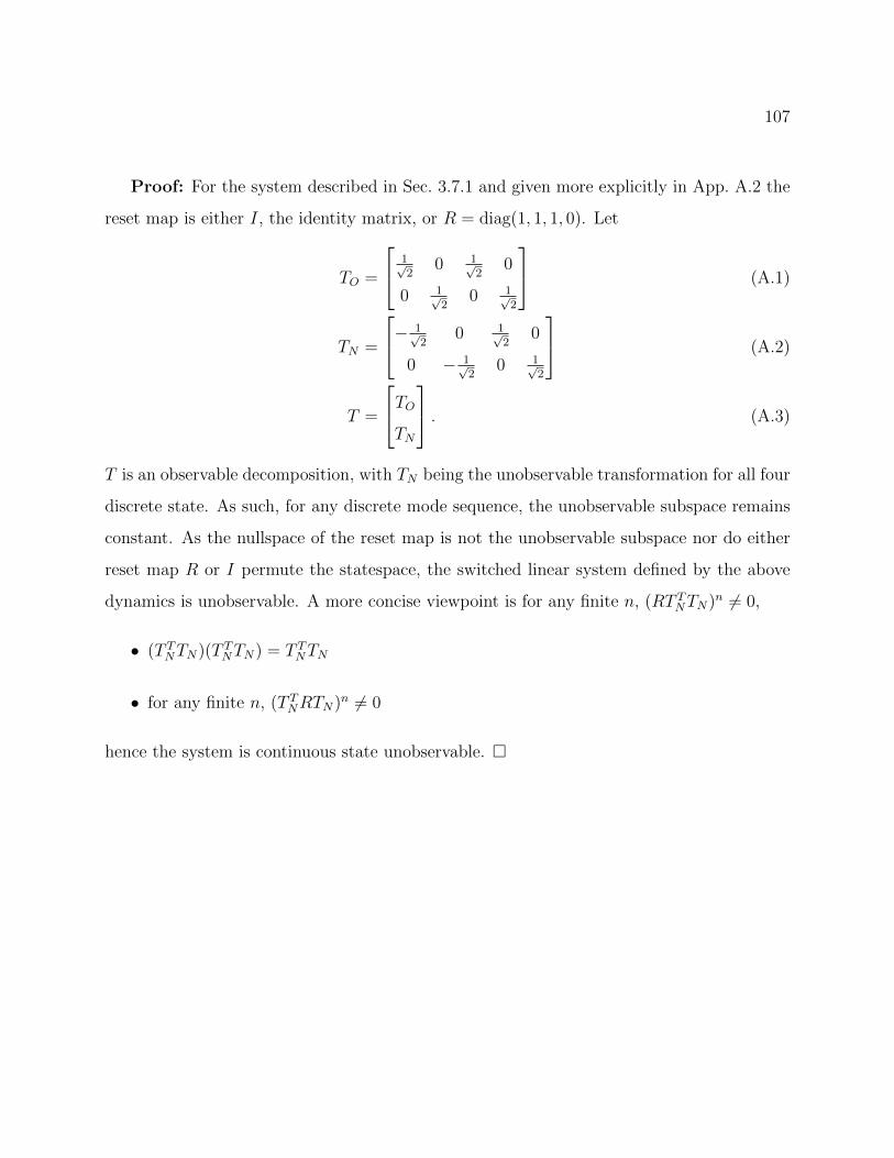
107

Proof: For the system described in Sec. 3.7.1 and given more explicitly in App. A.2 the

reset map is either I, the identity matrix, or R = diag(1, 1, 1, 0). Let

TO =

1√2

0 1√2

0

0 1√2

0 1√2

(A.1)

TN =

− 1√2

0 1√2

0

0 − 1√2

0 1√2

(A.2)

T =

TOTN

. (A.3)

T is an observable decomposition, with TN being the unobservable transformation for all four

discrete state. As such, for any discrete mode sequence, the unobservable subspace remains

constant. As the nullspace of the reset map is not the unobservable subspace nor do either

reset map R or I permute the statespace, the switched linear system defined by the above

dynamics is unobservable. A more concise viewpoint is for any finite n, (RT TNTN)n 6= 0,

• (T TNTN)(T TNTN) = T TNTN

• for any finite n, (T TNRTN)n 6= 0

hence the system is continuous state unobservable.