copyright by byung-soon min 2004 · the dissertation committee for byung-soon min certifies that...
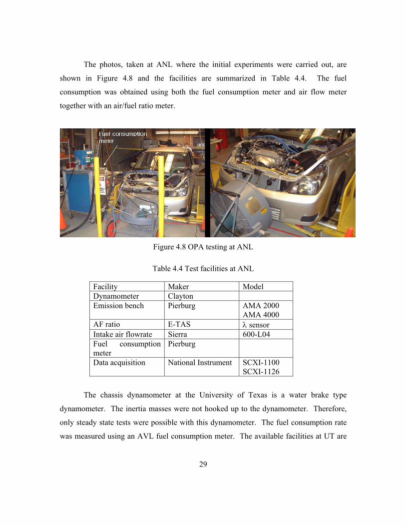
TRANSCRIPT

Copyright
by
Byung-Soon Min
2004

The Dissertation Committee for Byung-Soon Min certifies that this is the approved version of the following dissertation:
Analysis of the Fuel Economy Potential of a Direct Injection Spark Ignition Engine
and a CVT in an HEV and a Conventional Vehicle Based on In-Situ Measurements
Committee:
Ronald Matthews, Supervisor
Matthew Hall
Janet Ellzey
Ofodike Ezekoye
Robert Larsen

Analysis of the Fuel Economy Potential of a Direct Injection Spark Ignition Engine
and a CVT in an HEV and a Conventional Vehicle Based on In-Situ Measurements
by
Byung-Soon Min, B.S., M.S.
Dissertation
Presented to the Faculty of the Graduate School of
The University of Texas at Austin
in Partial Fulfillment
of the Requirements
for the Degree of
Doctor of Philosophy
The University of Texas at Austin
August 2004

Dedication
To my mother, Pyungja Shim and to my father, Kwanshik Min,
who love, encourage and support me.
and
Eunjin, Jiyoon and Dayoon

Acknowledgements
I owe an eternal debt of gratitude to Dr. Matthews for helping me with kindness and
patience. He is the best mentor I have ever had and I am very fortunate to have the
opportunity to work with him.
Thanks to the whole Argonne National Laboratory for its great welcoming and its
wonderful working environment. The contacts I made were really enriching both for the
work and human relationships: Bob Larsen, John Anderson, Mike Duoba, Justin Kern,
Henry Ng, Dave Shimcoski.
I would like to thank Cynthia Webb at the Department of Emissions Research of SwRI
for granting me a chance to use their facility.
Thanks to the rest of the members of my dissertation committee for helping send me on
my way a better person than I was when I got here:
Dr. Ezekoye, Dr. Ellzey, Dr. Matt Hall.
I thank my office partners: Myoungjin, Shinhyuk and Myoungjun. It was a great
pleasure to work with them. Additionally, I appreciate support received from
colleagues: Dohyung, Daejong and Younghoon.
Thanks to my wife Eunjin and kids Jiyoon and Dayoon, for love and life.
v

Analysis of the Fuel Economy Potential of a Direct Injection Spark Ignition Engine and a
CVT in an HEV and a Conventional Vehicle Based on In-Situ Measurements
Publication No.________________
Byung-Soon Min, Ph.D. The University of Texas at Austin, 2004
Supervisor: Ronald Matthews
A Toyota OPA was selected as a test vehicle as it has the components of
interest: a Direct Injection Spark Ignition (DISI) engine and a Continuously Variable
Transmission (CVT). In order to estimate the benefit of the DISI engine and CVT, a
2001MY Toyota OPA was tested to collect the engine and CVT maps using in-situ
measurement techniques. Two torque sensors were installed into the powertrain in the
vehicle for that purpose; one is between the engine and transmission and the other one
is installed on the driveshaft. The overall efficiency of the engine and transmission was
estimated using the measured torques and speeds during Phase 3 of the FTP cycle The
overall efficiencies of the engine at different operating modes including the lean and
stoichiometric combustion modes were compared to each other. The overall efficiencies
of the CVT are analyzed similarly. Finally, the measured steady state efficiency maps
and emissions maps were used to predict the fuel economy and emissions of an HEV
with the DISI engine and CVT.
vi
The FTP test for the test vehicle shows that Toyota has made a remarkable
improvement of tailpipe HC and NOx emissions with their second generation DISI
engine. The reduction of HC emissions is attributed to the improvement in the
combustion system using a slit nozzle injector. The dominant factor for NOx reduction
turns out to be the catalyst efficiency. Due to the increase in the catalyst capacity, the
average catalyst efficiency for NOx is improved from 67.5% to 89.9%.
The steady state characteristics of the DISI engine and CVT were collected
successfully using the in-situ mapping technique. The operating range of the lean
combustion was revealed. The maximum engine load for lean operation was 6 bar
BMEP and the maximum engine speed was 2750 rpm. The improvement in steady state
fuel consumption is about 20% at low speed and around 3 bar BMEP. The engine-out
HC emissions are 2~3 times more and the engine-out NOx emissions are one-half to
one-sixth of that in stoichiometric combustion mode.
The energy losses were calculated from the measured power flows. The engine,
the largest energy sink, consumes 62.3% of total energy loss during power mode and
additionally consumes 11.8% more during idling and braking. The CVT consumes 5.6%
and the vehicle consumes 20.2%. The overall efficiency of the engine, which is 29.3%
during the Hot 505 cycle, is improved to 32.7% with the change in combustion mode to
lean combustion. The resulting fuel economy improvement was measured as 5.7%.
Therefore, it can be concluded that the fuel economy benefit of the second generation
Toyota DISI engine over a PFI engine during Phase 3 of the FTP cycle is 5.7% which is
due to the 3.4% improvement in the overall engine efficiency.
The benefit of a DISI engine over a conventional SI engine in an HEV
application is found to be 4.2% in terms of composite fuel economy and 3.9% for the
Hot 505 cycle, which is less than that of 5.7% for a DISI engine in a conventional
vehicle. The overall engine efficiency improvement of a DISI engine in an HEV
application is 0.5 percentage points which is also less than that for a DISI engine in a
conventional vehicle application. This is because the engine is working in the high load
region due to the down-sized engine. This DISI engine operates primarily in
homogeneous charge mode for high load, and thus does not offer a large fuel economy
benefit. The HC emissions of both types of engines are similar to each other and the
NOx emissions of HEV with a DISI engine is 26% higher than that with an SI engine.
vii

TABLE OF CONTENTS
List of figures .........................................................................................................xi List of tables .........................................................................................................xiv Chapter 1 Introduction............................................................................................1
1.1 Background............................................................................................1 1.1.1 Development of the Hybrid Electric Vehicle ................................1 1.1.2 Attractions and barriers of DISI engines .......................................2 1.1.3 Efficient transmission ....................................................................5 1.1.4 In-situ measurement technique ......................................................5
1.2 Overview and goal of this project .........................................................6 Chapter 2 Test Vehicle Description and Preparation .............................................8
2.1 The 2nd generation Toyota D-4 and Super CVT ......................................8 2.2 Differences between the old and new D-4 system...................................9 2.3 D-4 combustion and emissions control system......................................11
Chapter 3 Methodology .......................................................................................14 3.1 Conventional vehicle ............................................................................14
3.1.1 Direct measurement of powertrain component efficiencies .......14 3.1.3 Power flow for each operation mode .........................................16 3.1.4 Component efficiencies .............................................................17
3.2 Hybrid Electric Vehicle ........................................................................18 Chapter 4 Experimental setup .............................................................................22
4.1 Sensor installation ................................................................................23 4.1.1 Torque sensor installation ..........................................................23 4.1.2 Temperature measurement .........................................................27
4.2 Facilities ...............................................................................................28 Chapter 5 FTP test results ....................................................................................32
5.1 Air/fuel ratio control .............................................................................32 5.2 Fuel economy ........................................................................................35 5.3 Emissions ..............................................................................................37
5.3.1 THC emission .............................................................................39 5.3.2 NOx emission .............................................................................41 5.3.3 CO emission ................................................................................43
5.4 Chapter summary ..................................................................................43 Chapter 6 Steady state test results ........................................................................45
viii
6.1 Steady state vehicle operation................................................................45 6.2 CVT efficiency.......................................................................................47 6.3 Air/fuel ratio distribution .......................................................................49 6.4 Fuel consumption...................................................................................52 6.5 Emissions ...............................................................................................53 6.6 Ignition and injection timing..................................................................56 6.7 Catalyst efficiency .................................................................................58 6.8 Chapter summary ..................................................................................60
Chapter 7 Overall efficiency measurements.........................................................61 7.1 Measured torque and power...................................................................61 7.2 Energy loss distribution .........................................................................66 7.3 Effect of additional parameters..............................................................67
7.3.1 Effect of warm-up .......................................................................67 7.3.2 Effect of shift mode ....................................................................70
7.4 Comparison with simulation ..................................................................73 7.5 Comparison with prior results................................................................77 7.6 Fuel economy potential of a DISI engine in a conventional vehicle .....78 7.7 Chapter summary ...................................................................................82
Chapter 8 Fuel economy and emissions of DISI engine powered HEV ..............84 8.1 Stock vehicle modeling..........................................................................85
8.1.1 Equinox model ............................................................................85 8.1.2 Simulation results .......................................................................87
8.2 HEV modeling .......................................................................................91 8.2.1 Component sizing .......................................................................91 8.2.2 HEV model for simulation ..........................................................93 8.2.3 Simulation results ........................................................................95
8.3 Chapter summary ...................................................................................98 Chapter 9 Summary and conclusions .................................................................100
9.1 Summary and conclusions ...................................................................100 9.2 Recommendations for future work ......................................................101
9.2.1 Finding a way to maximize the benefit of DISI engine in HEV application .....................................................................................102
9.2.2 Refinement of engine torque mesuring technique ....................102 9.2.3 Correlation of engine efficiency with the vehicle’s fuel economy
....................................................................................................103 Appendix A FTP test results................................................................................104
ix

Appendix B Steady state test results ...................................................................114 References ...........................................................................................................121 Vita ......................................................................................................................125
x

LIST OF FIGURES
Figure 2.1 Comparison of two D-4 combustion systems ................................................11 Figure 2.2 Combustion control scheme based on engine operating point (Numbers in
parenthesis indicate air/fuel ratio range) .............................................................12 Figure 2.3 OPA emissions control system ......................................................................13 Figure 3.1 Schematic diagram of power flow measurements .........................................15 Figure 3.2 Power flow during vehicle operation .............................................................16 Figure 3.3 Vehicle simulation model ..............................................................................18 Figure 3.4 Comparison of forward and backward models [27].......................................20 Figure 3.5 Block diagram of PSAT.................................................................................21 Figure 4.1 Positions for torque sensor installation ..........................................................23 Figure 4.2 Torque sensor used.........................................................................................24 Figure 4.3 Engine torque sensor installation ...................................................................25 Figure 4.4 Powertrain and vehicle after the torque sensor installation ...........................26 Figure 4.5 Axle shaft torque measurement system .........................................................26 Figure 4.6 Temperature measuring positions ..................................................................27 Figure 4.7 Location of catalyst temperature measurement .............................................28 Figure 4.8 OPA testing at ANL.......................................................................................29 Figure 4.9 OPA testing in UT..........................................................................................30 Figure 5.1 Comparison of air/fuel ratio control...............................................................33 Figure 5.2 Temperatures of the exhaust gas and catalysts ..............................................33 Figure 5.3 Engine operation for NOx regeneration.........................................................34 Figure 5.4 Comparison of engine operation for the OPA and Corona............................35 Figure 5.5 Fuel flowrate during FTP cycle .....................................................................37 Figure 5.6 Comparison of tailpipe emissions ..................................................................39 Figure 5.7 Source of THC difference between the OPA and Corona .............................40 Figure 5.8 Comparison of engine-out THC between the OPA and Corona during the
FTP cycle.............................................................................................................40 Figure 5.9 Source of NOx difference between the OPA and Corona .............................41 Figure 5.10 Comparison of NOx conversion efficiencies between the OPA and Corona
during the FTP cycle. The interval during which the efficiency is calculated is also illustrated......................................................................................................42
Figure 5.11 Source of CO difference between the OPA and Corona..............................43 Figure 6.1 Emissions during steady state engine operation ............................................46 Figure 6.2 Efficiencies of the CVT .................................................................................48 Figure 6.3 Estimated error in engine torque calculation .................................................49
xi

Figure 6.4 Operating points used in steady state tests.....................................................nn Figure 6.5 Measured lean combustion region .................................................................50 Figure 6.6 Air/fuel ratio distribution ...............................................................................51 Figure 6.7 Brake specific fuel consumption of the 2nd generation D4 engine ................52
Figure 6.8 Relative improvement in SFC (tricstoichiome
tricstoichiomelean
sfcsfcsfc −
×= 100 ) .......................53
Figure 6.9 Steady state emissions....................................................................................54 Figure 6.10 Change in EGR step according to load ........................................................55 Figure 6.11 Effect of combustion mode on the emissions during the last 140 seconds of
FTP Phase 1 and 3 ...............................................................................................56 Figure 6.12 Comparison of ignition timing.....................................................................57 Figure 6.13 Injection timing ............................................................................................57 Figure 6.14 Behavior of the catalysts ..............................................................................58 Figure 6.15 Catalyst conversion efficiencies for stoichiometry and lean combustion
modes...................................................................................................................59 Figure 7.1 Engine operating points during the Hot 505 cycle.........................................62 Figure 7.2 Measured engine and axle torques during the Hot 505 cycle ........................63 Figure 7.3 Measured power and energy during the Hot 505 cycle .................................64 Figure 7.4 Measured efficiencies of the engine and CVT during the Hot 505 cycle .....65 Figure 7.5 Change of the CVT efficiency according to the clutch state .........................66 Figure 7.6 Energy loss distributions................................................................................67 Figure 7.7 Comparison of the energy loss and efficiency according to the warm-up.....68 Figure 7.8 Change in fuel economy and contribution of each component......................69 Figure 7.9 Operating points according to shift modes ....................................................71 Figure 7.10 Energy losses at each component.................................................................72 Figure 7.11 Change of efficiencies by shift modes .........................................................72 Figure 7.12 Comparison of measured power flows with simulated................................75 Figure 7.13 Simulated energy loss distributions .............................................................76 Figure 7.14 Energy flow distribution ..............................................................................77 Figure 7.15 Comparison of the energy loss and efficiency according to combustion
mode ....................................................................................................................79 Figure 7.16 Effect of combustion mode on the overall engine efficiency and fuel
economy ..............................................................................................................80 Figure 7.17 Simulated engine operating points on BSFC map .......................................81
xii

Figure 7.18 Simulated fuel consumption and relative improvement during the Hot 505 cycle.....................................................................................................................82
Figure 8.1 Engine performance and efficiency used in simulation .................................86 Figure 8.2 Transmission efficiencies used in the simulations.........................................87 Figure 8.3 Screenshots for the simulation of conventional the Equinox.........................89 Figure 8.4 Screenshot of the simulation results...............................................................90 Figure 8.5 Characteristics of used motor.........................................................................94 Figure 8.6 Catalyst efficiency curve................................................................................94 Figure 8.7 Energy losses for each component.................................................................96 Figure 8.8 Engine operating points of an HEV ...............................................................97 Figure A.1 Engine operation during the FTP cycle.......................................................104 Figure A.2 Exhaust gas temperature during the FTP cycle...........................................107 Figure A.3 Catalyst temperature during the FTP cycle.................................................107 Figure A.4 Engine-out and Tailpipe THCs during the FTP cycle.................................108 Figure A.5 Engine-out and Tailpipe NOx during the FTP cycle ..................................109 Figure A.6 Engine-out and Tailpipe CO during the FTP cycle.....................................110 Figure A.7 Catalyst efficiencies during the FTP cycle..................................................111 Figure B.1 Brake specific fuel consumption maps........................................................114 Figure B.2 Brake specific HC maps ..............................................................................115 Figure B.3 Brake specific NOx maps............................................................................116 Figure B.4 Specific CO map .........................................................................................117 Figure B.5 MAP and volumetric efficiency ..................................................................118 Figure B.6 Ignition timing and injection timing............................................................119 Figure B.7 Exhaust and catalyst temperatures ..............................................................120
xiii
LIST OF TABLES
Table 1.1 Specifications of mass produced HEVs as of November, 2003........................2 Table 1.2 Factors contributing to the fuel economy benefit of a DISI engine ..................6 Table 2.1 Specifications of the OPA and Corona..............................................................9 Table 2.2 Difference in combustion system of new D-4 engine .....................................10 Table 2.3 Combustion control scheme ............................................................................12 Table 3.1 Measured Physical Quantities .........................................................................15 Table 3.2 Energy Losses for Each Mode.........................................................................17 Table 3.3 Comparisons of ADVISOR and PSAT [26]....................................................19 Table 4.1 Specifications of test fuel, EEE.......................................................................22 Table 4.2 Specifications of the engine torque sensor ......................................................24 Table 4.3 Test cells..........................................................................................................28 Table 4.4 Test facilities at ANL ......................................................................................29 Table 4.5 Test facilities at UT .........................................................................................31 Table 5.1 Fuel economy of the OPA and Corona (mpg) [28] .........................................36 Table 5.2 FTP emissions test results for the OPA (unit: g/mile).....................................38 Table 6.1 Measured physical quantities used to calculate the CVT efficiency...............47 Table 6.2 Lean combustion region of the 2nd generation Toyota D-4 engine .................50 Table 7.1 Fuel economies according to warm-up state ...................................................69 Table 7.2 Fuel economies according to shift mode.........................................................70 Table 7.3 Description of basic model parameters ...........................................................74 Table 7.4 Comparison of basic model parameters ..........................................................76 Table 7.5 Fuel economy for both combustion modes .....................................................78 Table 7.6 Summary of the benefit of lean combustion during the Hot 505 cycle...........81 Table 8.1 Specifications of the Equinox..........................................................................85 Table 8.2 Selected vehicle technical specifications in ChallengeX and PNGV
performance guidelines .......................................................................................88 Table 8.3 Comparison of simulation results with the vehicle technical specifications...90 Table 8.4 Criteria for component sizing..........................................................................91 Table 8.5 Combination of engine/motor/battery to satisfy performance guidelines .......92 Table 8.6 Configurations and components used..............................................................93 Table 8.7 Fuel economy simulation results .....................................................................95 Table 8.8 Contribution of each factor on the fuel economy improvement due to the
hybridization........................................................................................................96 Table 8.9 Dwell time in lean combustion mode of DISI engine during 505 cycle .........98
xiv

Table 8.10 Simulated emissions of HEVs with SI and DISI engines (g/mile)................98
xv

CHAPTER 1: INTRODUCTION
The Partnership for a New Generation of Vehicles (PNGV) identified the Hybrid
Electric Vehicle (HEV) as a key configuration to achieve significant fuel economy
improvements [3]. The FreedomCAR Partnership, the successor to the PNGV, continues
to support the electric propulsion systems applicable to both fuel cell and internal
combustion/electric hybrid vehicles. The benefit by hybridization depends on the balance
between improvements in hybrid designs and improvements of powertrain components.
The engine in the HEV is the least efficient component in the powertrain so the
development of an efficient engine is more effective than improvements to the other
components of an HEV drivetrain. Therefore, the use of an efficient engine and
transmission is also important in HEVs as well as in conventional vehicles.
In the present Ph. D. research, the fuel economy benefit of DISI engine over the
Port Fuel Injection engine is investigated in both a conventional and a hybrid electric
vehicle. The benefit of a Continuously Variable Transmission (CVT) is also researched.
For that purpose, the 2001 MY Toyota OPA was selected to be tested as a vehicle with
the state-of-the-art DISI engine and CVT. To overcome the difficulty of benchmarking
tests, an in-situ measurement technique was developed and used. The following sections
address the basic information for the important issues in this research.
1.1 BACKGROUND
1.1.1 Development of the Hybrid Electric Vehicle
As the hybrid system is regarded as a promising system that can reduce energy
consumption and emissions regardless of using the different power plants such as the
diesel engine and fuel cell, the development of the HEV system is a general trend of the
automotive industry. As a first step, Toyota launched the Prius in 1997 and added two
more models in 2001 – the Estima Hybrid minivan and Crown mild-hybrid. Honda has
1

two HEV models – Insight and Civic. The specifications of the mass produced HEVs are
shown in Table 1.1.
Table 1.1 Specifications of mass produced HEVs as of November, 2003
Manufacturer Vehicle Configuration Engine Transmission Prius Power split SI ECVT Estima Parallel
(2 motor 4WD)SI CVT
Toyota
Crown Parallel DISI AT Insight Parallel Lean burn MT/CVT Honda Civic Parallel Lean burn MT/CVT
It is seen in this table that the parallel type is the majority of current HEVs. The
potential for fuel economy gains due to vehicle hybridization can be estimated on the
three elements [3]: the reduction of engine idling, the recovery of braking energy and the
capability of high efficiency operation control. However, according to Toyota, the
parallel type HEV is somewhat unfavorable for the high efficiency operation. A common
misconception of how a hybrid works is the dated thermostat concept [31]. That is, a
small engine is operating at a constant output power at its maximum efficiency point,
providing the averaging energy with a battery acting as a load follower. One problem of
this concept is that some trips need a higher than average load condition for a long time
period. Therefore, the improvement of the efficiency of each powertrain component is
essential for an efficient HEV.
1.1.2 Attractions and barriers of DISI engines
Current lean burn engines, both compression and spark ignition, have high
potential efficiencies. The Direct Injection Compression Ignition (CIDI) engine has
higher potential than the spark ignition engine. However, the Direct Injection Spark
Ignition (DISI) engine is also attractive due to its emissions potential over the CIDI
engine and fuel economy potential over the PFI gasoline engine. Thus, The important
viewpoints for the adoption of the DISI engine are how much benefit can be obtained and
if the DISI engine can meet the strict emissions regulations. Zhao and coworkers [41] 2

summarized the major factors contributing to the improved BSFC of the DISI engine
over that of a conventional PFI engine as follows;
• Decreased pumping losses due to unthrottled part load operation using overall
lean mixtures
• Increased knock limited compression ratio due to low end gas temperature
• Increased cooling of the intake charge due to in cylinder injection during
induction
• Increased cycle efficiency due to the incrementally higher specific heat ratio
of lean mixtures
• Decreased cylinder wall and combustion chamber heat loss due to stratified
combustion
In the stage of decision making, it is necessary to evaluate the actual benefit that
can be drawn from the adoption of a DISI engine. There are several arguments regarding
this matter. Karl and coworkers [20] said that the stratified GDI engine can reduce the
fuel consumption by 20~25% at part load with the optimized gas cycle, heat transfer and
geometric configuration. A 25% increase in fuel economy potential is reported by Wojik
and Fraidl[39]. The theoretical potential of fuel economy is reported as 20% at part load
and 35% at idle by Fraidl and coworkers [14]. Regarding the fuel economy benefit in the
vehicle, Kume and coworkers [25] said that the vehicle fuel economy can be improved by
35%. According to the recent publication by Alkidas and El Tahry [1], the potential of
the DISI engine is overestimated and its advantage in the FTP cycle is only 15%.
However, GM’s Fritz Indra said in the report of Dan Carney that, in production, the
engine lost 1% because of the wide range of operating conditions and margin of mass
production. In addition, the condition around the spark plug is not ideal. Finally, the
gain ends up with a 6~7% benefit for a stratified charge DISI engine [7]
A DISI engine has the barriers into the market as well as the attraction. The first
barrier is a higher level of emissions. At a constant engine speed of 2000 rpm, Matthews
and coworkers [29] found that the early injection mode (homogenous charge near
stoichiometric) engine-out HC Emission Index (g/kgfuel) was about twice as high as that 3

for a comparable PFI engine. The HC Emission index for late injection was higher by a
factor of up to four. Brehob and coworkers [6] measured the brake specific HCs
(BSHCs) to be ~25% higher in early homogeneous charge mode than those from a
comparable PFI engine. For late injection, the brake specific HCs increase monotonically
with increasing air/fuel ratio up to 3 times.
On the contrary, the NOx emissions in the stratified charge lean mode is reported
as less than that of the homogeneous charge stoichiometric mode [34]. However, for the
DISI designed to operate with lean combustion, the conventional three way catalyst can
not be used effectively to remove the NOx. Therefore, other techniques for in-cylinder
NOx reduction or after-treatment are necessary. As an in-cylinder NOx reduction
technique, EGR is widely used. For a DISI engine using charge stratification, stable
combustion is possible with a high level of EGR because the mixture near the spark plug
is not affected by diluted exhaust gas. A comparison of the effect of EGR on the NOx
reduction reported by Kuwahara and coworkers [26] shows that a larger NOx reduction
can be realized for DISI than that for PFI.
A number of technologies are being explored for a NOx reduction catalyst for
lean exhaust gas. Two catalyst concepts have entered into the market as follows [24].
• The continuously reducing Iridium catalyst using HC in lean burn phases as
selective reductant for NOx
• The non-continuously reducing NOx storage catalyst which stores NOx in lean
burn phases and reduces NOx to harmless N2 in rich or stoichiometric operation
mode
Only the NOx storage catalyst has the potential to meet the stringent U.S.
emissions standards but it needs to develop not only the catalyst but also a sophisticated
additional engine management. In addition, the fuel originated sulfur compounds are
known to reduce the effectiveness of this catalyst. Therefore, the De-NOx catalyst with
more potential for sulfur tolerance or sulfur free fuel is necessary.
4
1.1.3 Efficient transmission
Another feature of the OPA is its CVT. The Super CVT is Toyota’s first steel
push-belt and pulley continuously variable transmission, manufactured in-house and
using a Dutch Van Doorne Transmissie belt. Toyota boasted that the newly introduced
Super CVT realized both good fuel economy and high driving performance [30].
According to Kluger and Long [21], the overall efficiency of a belt type CVT is
84.6% which is less than the efficiency of manual and automatic. However, the major
advantage of a CVT is that it allows the engine to operate in a more fuel efficient region.
Thus the combination of a CVT and conventional engine can improve the typical
powertrain’s fuel economy by 5~10%.
1.1.4 In-situ measurement technique
Most automotive manufacturers have been doing benchmarking tests and
comparing the performance and fuel economy of competing vehicles to devise
countermeasures. However, the testing of other maker’s engines or transmissions has
become difficult because the control system of the engine is integrated with that of the
transmission and vehicle. In addition to that, the engine control computer controls not
only the injection and ignition but also VVT, EGR and so on. Especially for DISI
engines, it controls the throttle valve and swirl valve. The recent ECU communicates
even with the brake and ABS. As a result of that, even a little modification of the engine
can induce a complete malfunction of engine control.
Therefore, the best way of benchmarking testing is doing that without any
modification to the powertrain. To do that, it is necessary to install a torque sensor
between the engine and transmission in a vehicle. There have been several attempts to
put a torque sensor in such a position. Duoba and coworkers [12] attempted and
succeeded in measuring engine-out torque to examine the powertrain of the Prius, the
first HEV in the market. In another publication of them [13], an axle shaft torque sensor
was installed on an Insight. The characteristics of two kinds of HEVs were assessed and
5

compared. Another example of in-situ measurements was published by Corsetti and
coworkers [9]. They refined the torque measuring system in a vehicle to supplement the
engine dynamometer development and validation of an ECM torque model.
1.2 OVERVIEW AND GOAL OF THIS PROJECT
In the present PhD research, the actual fuel economy benefit of a DISI engine and
CVT was evaluated in terms of overall efficiency for a driving cycle and fuel economy as
a result of that for both a conventional vehicle and an HEV. In the conventional vehicle,
the efficiency of the DISI engine will be measured and compared with the same engine
operating in stoichiometric mode in the same vehicle. The itemized factors on the fuel
economy benefit of a DISI engine was reported by Kume and coworkers [25] and Alkidas
and El Tahry [1] and tabulated in Table 1.2.
Table 1.2 Factors contributing to the fuel economy benefit of a DISI engine
Factors By [Kume and coworkers, 1996]
By [Alkidas and Tahry, 2003]
Reduced pumping loss 15% 10.2% Higher specific heat 5% 7.5% Reduced thermal dissociation 2% Compression ratio 4% 3.1%
Positive
Reduced heat loss 5% 2% Lower combustion efficiency -4% Negative Higher friction -3.9%
Total 30% 15%
By means of a scan tool, the DISI engine’s operating mode was manipulated to
operate in homogeneous stoichiometric mode. With the same engine hardware and
different mixture preparation, we can examine the all the factors in Table 1.2 except for
the compression ratio. Thus, according to Alkidas and El Tahry [1], the fuel economy
benefit should be about 12%. The power flow through each powertrain component was
measured and integrated to be the total energy flow. From this energy flow, the overall
and average efficiencies of the engine and transmission will be obtained. The
6

comparison between the conventional gasoline engine and the DISI engine in the same
vehicle was accomplished by controlling the second generation Toyota D-4 DISI engine
to operate either i) in homogenous charge, throttled mode for all engine operating
conditions or ii) as a DISI engine.
Through the vehicle testing, steady state efficiency and emissions maps were
collected and used in an HEV simulation. For evaluation of the benefits of the DISI
engine and CVT in an HEV, a simulation method was used because it is not possible to
build a physical HEV as necessary to allow direct experimental measurement. As a
simulation tool, ADVISOR (Advanced Vehicle Simulator) and PSAT (Powertrain
System Analyst Toolkit) were used. The ADVISOR is one of the most well known tools
for vehicle modeling, developed in the National Renewable Energy Laboratory (NREL)
and programmed in MATLAB/Simulink. The PSAT is developed in Argonne National
Laboratory (ANL) and programmed in MATLAB/Simulink, too.
In summary, three primary deliverables are expected from this dissertation:
• A comparison of the fuel economy of a conventional gasoline and a DISI engine
in the same vehicle operating over a transient driving cycle.
• A comparison of engine/drivetrain/vehicle energy distributions for the same
vehicle with a conventional gasoline engine and a DISI engine, as averaged for
operation over a transient driving cycle.
• Prediction of fuel consumption and emissions for a DISI engine in an HEV.
7

CHAPTER 2: TEST VEHICLE DESCRIPTION AND PREPARATION
This chapter describes the test vehicle used in this study. The major reason to
select the OPA as the test vehicle is that it has the 2nd generation D-4 engine of Toyota.
The differences of the 2nd generation and the 1st generation D-4 engine are explained to
help the understanding of the differences in measured emissions that will be mentioned in
the later chapters.
2.1 THE 2ND GENERATION TOYOTA D-4 AND SUPER CVT
A 2001 model year Japanese market Toyota OPA is used as the test vehicle. The
University of Texas previously tested a vehicle, a 1998 Corona Premio, equipped with
the 1st generation D4 and automatic transmission. Stovell and coworkers [35] measured
the fuel economy and emissions and compared with those of a 1999 Corolla with a PFI
engine. In this previous collaboration between UT and Argonne National Labs, it was
shown that high tailpipe emissions of NOx and, to a lesser extent, HCs were the biggest
barriers to introduction of vehicles with DISI engines into the U.S. market. Furthermore,
periodic regeneration of the lean NOx trap/catalyst and an extended period of
homogenous stoichiometric operation to light-off this catalyst at the beginning of the FTP
penalized fuel economy. Additionally, it was shown that tailpipe NOx emissions were
high during acceleration and high speed cruises. It was postulated that use of a DISI in
an HEV might overcome the emissions barriers while improving fuel economy.
Toyota has developed a new generation D-4 engine with an improved combustion
system and launched several vehicles with it. Table 2.1 shows the difference of
specifications between the vehicles with the 1st and 2nd generation D-4 engine. From this
table we can see that the OPA shows better fuel economy and emissions due to
improvement in the combustion system.
8

Table 2.1 Specifications of the OPA and Corona
Corona Premio G OPA 2.0a 2WD Weight 1200 kg 1250 kg Total Weight 1475 kg 1525 kg Fuel consumption (10-15 mode) 17 km/L 17.8 km/L Vehicle
Emission rating Japan 1978 regulation certified* J-TLEV certified*
Name 3S-FSE 1AZ-FSE Displacement volume 1998 cc ←
Valve train VVT-i VVT-i Fuel pressure 12 MPa ← Intake port Helical + Straight Straight Rated Power/Speed 107 kW/ 6000rpm 112 KW/6,000 rpm Max Torque/Speed 196 N-m/ 4400rpm 200 N-m/4,000 rpm
Engine
EGR Yes Yes Transmission Type ECT(4AT) Super CVT
* 70% reduction in regulation
2.2 DIFFERENCES BETWEEN THE OLD AND NEW D-4 SYSTEM
The major differences between these two D-4 systems are shown in Table 2.2 and
Figure 2.1.
The original D-4 relies on the incoming air’s powerful swirl motion to create
charge stratification, gathering a fuel-rich portion around the spark plug. Swirl is
generated by closing the straight port letting air enter through the open helical port. The
swirl control valve (SCV) and helical port are combined with a deep, asymmetrical heart
shaped bowl in the piston to obtain charge stratification. The bent intake port and deep
bowl designs impede efficient filling in the engine’s high load, homogeneous charge
operation, limiting maximum torque and power.
The new D-4 combustion system uses the mixture’s inertial dynamics versus the
original version’s swirl flow. The key to the system is the new “slit” injector design.
9

From this novel design, fuel is injected in a solid, fan-like pattern versus the previous
hollow cone “casting net” pattern.
Table 2.2 Difference in combustion system of new D-4 engine
Old system New system Injector Cone nozzle Slit nozzle
Flow Swirl (Weak tumble) Intake Port Helical & straight port 2 straight ports
Piston bowl Deep and asymmetrical heart shaped
Shallow and symmetrical shell (oval) shaped
Mixture preparation By charge motion By spray’s own energy
Figure 2.1 shows a schematic of mixture preparation of the two combustion
systems [18]. In the old system, a helical shaped swirl intake port is used to produce an
optimum swirl in the cylinder by variable controlled swirl control valve. Pistons with a
concave bowl and high pressure fuel injection system provide a fine fuel-air mixture in
the combustion chamber. Compared to the previous spray, the new spray has large
penetration and uniform fuel distribution [23].
Due to these improvements, the new D-4 system achieved stratified combustion
over a larger range of operating conditions and higher output performance compared to
the previous one [16]. In addition to the advantage in power and enlarged stratified
combustion region, the engine-out THC and NOx are reduced by 20~30% [18] and the
robustness of engine control is improved. The catalyst of the OPA is also improved. The
new one has 1.5 times the NOx storage capacity of the previous type and its sulfur
resistance has been increased. The amount of tailpipe NOx after durability testing is
about one-third of that with the conventional catalyst [15]. The combined improvement
in combustion system and catalyst system results in far better emissions rating. The
previous Corona was certified for 1978 Japanese regulation 1 whereas the OPA was
certified for J-TLEV2 which is only 30% of 1978’s regulation.
1 HC: 0.25 g/km, CO: 2.1g/km, NOx: 0.25g/km 2 HC: 0.06 g/km, CO: 0.67g/km, NOx: 0.06g/km
10

Old system New systemOld system New system
Figure 2.1 Comparison of two D-4 combustion systems
2.3 D-4 COMBUSTION AND EMISSIONS CONTROL SYSTEM
The engine control computer determines the optimum combustion scheme based
on the engine operating point determined from various sensors as shown in Figure 2.2. It
switches the control scheme by controlling injection timing and quantity, throttle position
and EGR valve opening.
11

torque
Engine speed
Road load curve
Homogeneous(12~15)
Weak stratified(15~30)
Stratified(17~50)
100km/h
torque
Engine speed
Road load curve
Homogeneous(12~15)
Weak stratified(15~30)
Stratified(17~50)
100km/h
Figure 2.2 Combustion control scheme based on engine operating point (Numbers in
parenthesis indicate air/fuel ratio range)
Table 2.3 shows the combustion control schemes. When the engine load is above
a certain load threshold, the engine is working in the homogeneous charge mode. Other
homogeneous charge control modes are during cold start, brake control and NOx control.
During brake control, the engine goes stoichiometric throttled to supply a significant
amount of negative pressure (vacuum) to the brake booster. For control of NOx in NOx
the storage reduction catalyst, the engine control should be stoichiometric or rich to
supply the reduction agent (HC and so on).
Table 2.3 Combustion control scheme
Control Combustion A/F ratio Injection timing Operating condition
Stratified 50~17 Compression Low load Lean control Weak Stratified
(2 stage) 30~15 Compression & Intake Middle load
High load Cold Start Brake control
Stoichiometric control Homogeneous 15~12 Intake
NOx control
12

The OPA has two catalysts as shown in Figure 2.3. In addition to the three way
catalyst, a NOx storage reduction catalyst is installed downstream of the 3 way catalyst.
It traps NOx as nitrate during lean operation. The stored NOx is reduced to N2 in
homogeneous control regeneration mode occurring once every 30~50 seconds. The
reduction agents, such as HC in the stoichiometric/rich products of combustion are used
to reduce the stored NOx.
Figure 2.3 OPA emissions control system
13
CHAPTER 3: METHODOLOGY
This chapter describes the methodology used to estimate the benefit of DISI
engine in two types of powertrains, conventional vehicle and HEV. For the conventional
vehicle, an experimental method was used and a simulation was performed to support the
experimental results. The procurement of the vehicle with state-of-the-art DISI engine
made it possible to estimate experimentally this benefit but a different methodology was
necessary for HEV. A virtual HEV was built and the resulting fuel economy, emission
and performances were evaluated using a simulation method. The experimental
approach, analysis method and simulation method are explained in this chapter.
3.1 CONVENTIONAL VEHICLE
Conventional methods to evaluate the factors on fuel economy are fuel economy
test in driving cycle or collecting a 2 dimensional specific fuel consumption map from
component testing. However, as the fuel economy of a vehicle is the combined result
from all factors, it is not easy to distinguish the contribution of a specific factor from
vehicle fuel economy testing. Also, the specific fuel consumption map can give only a
clue to explain a difference in efficiency, not the overall efficiency itself. Therefore, in
order to directly evaluate and compare the efficiency, it is necessary to directly measure
the efficiency of the specific component during an actual driving cycle.
3.1.1 Direct measurement of powertrain component efficiency
In this research, the fuel consumption and power flow between the major
powertrain components were collected during Phase 1 and Phase 3 of the FTP cycle. To
assess the power flow through the major components, the fuel flow rate into the engine
and the speeds and torques out of the engine and out of the CVT were measured as shown
in Figure 3.1.
14

Figure 3.1 Schematic diagram of power flow measurements
The physical quantities measured for this experiment are summarized in Table
3.1. The fuel flowrate was deduced from the measured air flowrate and measured AF
ratio. The accuracy of the fuel flow calculation was confirmed by comparing it with that
of a direct fuel consumption meter during steady state tests.
Table 3.1 Measured Physical Quantities
Power Formulae Physical quantity Instrument Air flowrate Laminar flow meter
valueheatingLowerFA
flowrateair×
/ A/F ratio λ sensor
Fuel power
valueheatingLowerflowratefuel × Fuel flowrate AVL fuel consumption
meter Torque Engine power engineengine ωτ × Speed HBM T10F
Torque SDI sensor Axle power axleaxle ωτ × Speed CVT speed signal
15
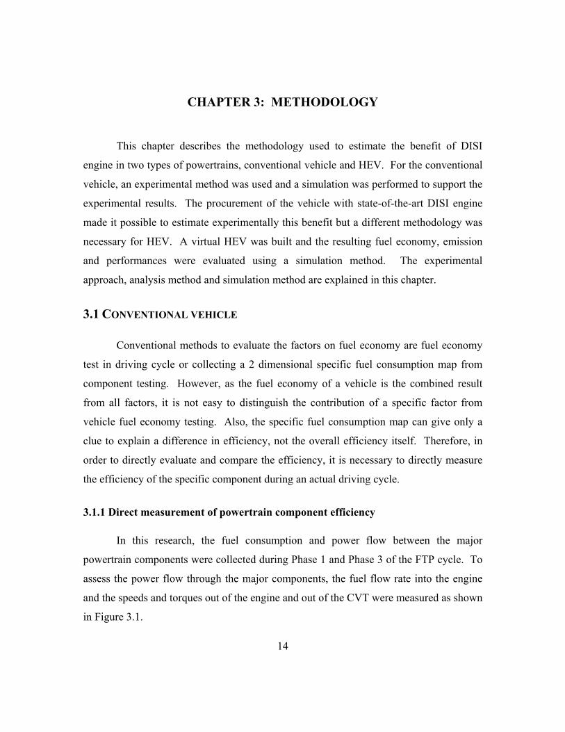
3.1.2 Power flow for each operation mode
The function of the powertrain in a vehicle can be defined as conversion of the
chemical energy of the fuel into rotational mechanical energy and transmission of this
energy to kinetic energy of the vehicle. Therefore, the loss of energy occurs during this
conversion and during transmission. Therefore, to analyze those losses of energy, the
vehicle operating mode should be defined first as shown in Figure 3.2.
Fueltank Engine Drive
train VehicleEfuel Eengine ECVT
Chemicalenergy
Mechanicalenergy
Mechanicalenergy
(a) Engine power mode
Fueltank Engine Drive
train VehicleEfuel Evehicle
Chemicalenergy
Mechanicalenergy
Mechanicalenergy
(b) Standby mode
ECVT
Fueltank Engine Drive
train VehicleEfuel Eengine ECVT
Chemicalenergy
Mechanicalenergy
Mechanicalenergy
(a) Engine power mode
Fueltank Engine Drive
train VehicleEfuel Evehicle
Chemicalenergy
Mechanicalenergy
Mechanicalenergy
(b) Standby mode
ECVT
Figure 3.2 Power flow during vehicle operation
In Figure 3.2, the engine power mode means the engine power is transmitted to
the vehicle for acceleration, cruising and powered deceleration. Therefore, the efficiency
of the engine and drivetrain are important in this mode. During braking, the kinetic
energy is lost if there is no regeneration device as in a hybrid electric vehicle. Moreover,
fuel must be supplied to the engine to maintain stability. Accordingly, the overall
efficiency of the engine is 0% and all the fuel energy supplied to the engine is lost during
the standby mode.
16

Table 3.2 Energy Losses for Each Mode
Mode Loss component Energy loss Engine loss Fuel energy – Engine output CVT loss Engine output – CVT output
Engine power mode Vehicle loss Road load + Acceleration
Idle loss Fuel energy Stand-by mode Braking fuel loss Fuel energy
In this analysis, the energy loss and efficiency of each component were
investigated according to the vehicle modes and energy losses, as summarized in Table
3.2. The tests are performed with the engine in stratified charge unthrottled mode as well
as in homogeneous throttled mode. As results of tests in two different combustion
modes, the benefit of DISI engine is investigated.
3.1.3 Component efficiencies
Based on the measured fuel flowrate from the fuel tank and torque and speed of
the engine and transmission, the overall efficiency can be calculated from the following
formulae. For the various conditions of the engine and the vehicle, the overall
efficiencies from the following formulae can be obtained. The efficiency of the DISI
engine is obtained by running the vehicle at the normal operating mode and that of the
PFI is obtained by manipulating the mode into the homogenous stoichiometric mode.
Then, the overall efficiencies of both the lean burn mode and the homogenous mode can
be compared.
∫∫∫∫
⋅
⋅=
⋅=
emodpower engineengine
emodpower CVTCVT
CVT
emodpower fuel
emodpower engineengine
engine
dt
dt
dt)LHV(m
dt
ωτ
ωτη
ωτη
& (1)
17

3.2 HYBRID ELECTRIC VEHICLE
The benefit of a DISI engine in a conventional vehicle can be estimated by actual
vehicle testing. Similar tests could be performed on an HEV. However, it was not
possible to build a vehicle for the purpose of this research. Therefore, a virtual HEV and
a simulation tool which can predict the fuel economy and emissions are necessary. The
required functions of the simulation tool are as shown in Figure 3.3. The simulation
program should predict the fuel economy and emissions from the input data such as the
vehicle resistance and powertrain efficiency and engine emissions maps and the cycle
that the vehicle needs to run on. It also has various libraries of vehicle models from the
conventional vehicle to the various types of HEVs such as series, parallel and power-
split.
Fuel economy (MPG)
Emission (g/mile)
Configuration
Conventional
Hybrid Electric Vehicle
Vehicle resistance
–Mass
–Drag resistance
–Rolling resistance
Powertrain
–Efficiency
–Emissions
Cycle
–FTP, US06, SC03
–Japan 10-15
Vehicle modelInput data Output
Fuel economy (MPG)
Emission (g/mile)
Configuration
Conventional
Hybrid Electric Vehicle
Vehicle resistance
–Mass
–Drag resistance
–Rolling resistance
Powertrain
–Efficiency
–Emissions
Cycle
–FTP, US06, SC03
–Japan 10-15
Vehicle modelInput data Output
Figure 3.3 Vehicle simulation model
ADVISOR (ADvanced VehIcle SimulatOR) and PSAT (Powertrain Systems
Analysis) were used as the simulation tools as shown below.
ADVISOR version 2002
PSAT version 5.1 Non-proprietary version
18

Brief descriptions for ADVISOR and PSAT are shown in Table 3.3. Both tools
are based on a Bond graph model [19]. There are effort and flow for each component
model. The efforts and flows change as they pass through the components.
Table 3.3 Comparisons of ADVISOR and PSAT [32]
PSAT ADVISOR Model Map based model
• For maximum/minimum characteristics • Efficiency and emissions
Bond graph model
• Mechanical Component
o Effort = Torque o Flow = Speed
• Electrical Component o Effort = Voltage o Flow = Current
History • 1995 by USCAR (Contract to SwRI)
• 1999 transferred to ANL
• 1994 by USCAR (Contract to NREL)
Primary difference • Forward facing • Backward facing
19
The main difference between the two simulation tools is that PSAT is based on a
forward facing model and ADVISOR is facing backward, as shown in Figure 3.4. The
backward model means the desired vehicle goes from the vehicle model back to the
engine to finally find out how each component should be used to follow the speed cycle.

Instead, the forward model used in PSAT goes from the driver. The driver determines
the required power to drive the vehicle as close to the given cycle as possible. Then this
power passes through the clutch, transmission, final drive, wheel and finally to the
vehicle (i.e., the road). The efficiencies and dynamic effects of each component model
affects the flows of speeds and torques between the component models.
(a) Backward facing model
(b) Forward facing model
Figure 3.4 Comparison of forward and backward models [44]
The forward facing model is closer to the actual operation of the vehicle. Its
advantages over the backward facing model can be summarized as follows [44];
• More realistic prediction for the transient component behavior and vehicle
response
• Consistent with industry design practice
• Allows for the development of control strategies that can be utilized in
hardware-in-the-loop or vehicle testing
20
In this research, PSAT and ADVISOR were used for the conventional vehicle
simulation. The predictions of both programs were compared with the measured results.
For the simulation of the HEV, PSAT was selected due to the advantages mentioned

above. Figure 3.5 shows an example of the block diagram of PSAT. The controller
model determines the operation of each component based on the accelerator and brake
pedal position from the driver model. The driver sees the vehicle speed of a given
driving cycle and actual vehicle speed and controls accelerator and brake pedals. The
controller determines the load of the engine, clutch engagement, gear shifting, brake
on/off and the usage of the motor.
Figure 3.5 Block diagram of PSAT
21

CHAPTER 4: EXPERIMENTAL SETUP
For this project, the test vehicle, a 2001 OPA, was imported directly from Japan.
The break-in time period was dictated by the catalyst’s aging requirement needed for
emissions certification. Due to time and cost, a dyno-controlled AMA cycle break-in
period was not done on the vehicle. Instead a simulated AMA cycle was mapped out
using the streets and highways of Chicago and the surrounding areas. Several workers at
ANL, including this author, drove the vehicle until the 4000 miles were accumulated.
Special concern regarding the contamination of the lean NOx trap catalyst
required the use of special fuel during not only the actual testing but also the break-in
period. A gasoline with high sulfur concentration, which is usually available in any gas
station, may affect dramatically the lean NOx trap catalyst’s efficiency. Inappropriate
use of fuel would result in an inaccurate representation of the tailpipe emissions of the
production vehicle. The fuel used throughout this research is commercially known as
EEE. The EEE fuel is an unleaded low sulfur fuel used as a certification gasoline. Its
specifications are presented in Table 4.1.
Table 4.1 Specifications of test fuel, EEE
Specification Units Value Gravity °API 59.3 Density kg/liter .741 Reid vapor pressure psi 9.2 Hydrogen/Carbon ratio mole/mole 1.806 Oxygen wt % <0.05 Sulfur wt % 0.0035 Lead g/gal <0.01 Phosphorus g/gal <0.0008 Aromatics vol % 29.2 Olefins vol % 0.7 Saturates vol % 70.1 Net heating value BTU/lb 18430 Research octane number 97.6 Motor octane number 88.5
22

4.1 SENSOR INSTALLATION
A special technique of sensor installation used in the present research is torque
sensor installation in the vehicle so that it can be tested on the chassis dynamometer. The
engine and axle shaft torque measuring methods are explained. The installation of
thermocouples on the catalyst is explained as well.
4.1.1 Torque sensor installation
Two kinds of torque sensors were installed to measure the power output of the
engine and CVT. In the present experiments, an engine torque sensor was installed
between the engine and CVT, as shown in Figure 4.1, so that the engine-out torque and
speed could be measured during chassis dynamometer testing.
EngineCVT
EngineCVT
Engine torque sensor
Axle shaft torque sensors
Engine torque sensor
Axle shaft torque sensors
Figure 4.1 Positions for torque sensor installation
Though the apparent functions of both torque sensors are the same, the torque
sensors and installations of them are different from each other. An engine torque sensor
was purchased from HBM GmbH and installed between the engine and CVT. The
necessary parts and modifications were accomplished at ANL. For the measurement of
axle shaft torque, the axle shafts were take out from the vehicle and sent to the Sensor
23

Development Inc.. This sensor company attached strain gauges on the axle shafts and
sent them back to ANL with a telemetry system.
The engine torque sensor is composed of a rotor and stator as shown in Figure
4.2. The rotor is installed between the crankshaft and torque converter and rotates
together with them. The stator is a kind of signal receiver and was installed on the
housing located between the engine and transmission case. The specifications of the
torque sensor are shown in Table 4.2.
rotor
stator
rotor
stator
Figure 4.2 Torque sensor used
Table 4.2 Specifications of the engine torque sensor
Manufacturer HBM Model T10F-200 Measuring system Strain gauge Load limits 200 N-m Limit torque 400 N-m Breaking torque 800 N-m Maximum speed 8000~15000 rpm Temperature range 10~60 °C Signal transfer Non-contact Output signal Voltage, frequency
24

This torque sensor has a finite thickness so the total length of the powertrain must
be increased. In the case of this OPA, the total length increased by 3 inches. There are
two kinds of work necessary for the torque sensor installation as shown below.
• Sensor work: Machining the adapter and sensor housing
• Engine room work: Modification for increased powertrain length
Photos of the torque sensor installation are shown in Figure 4.3. At first, the
powertrain was taken out from the vehicle. Then, the sensor work and engine room work
proceeded separately.
(a) Sensor work
(b) Engine room work
Figure 4.3 Engine torque sensor installation
25

After the sensor work and engine room work, the powertrain was installed into the
vehicle to be ready to go. The completed powertrain and vehicle are shown in Figure 4.4.
There were additional modifications done due to the sensor installation. The engine room
cover and the brake booster were removed. Thus, the tests were done without the brake
booster.
(a) Assembled powertrain (b) Vehicle after the powertrain installed
Figure 4.4 Powertrain and vehicle after the torque sensor installation
For the measurement of axle shaft torques, a strain gauge was attached on the
surface of each axle shaft. The axle shaft torque measurement system is shown in Figure
4.5.
Figure 4.5 Axle shaft torque measurement system
26

As the sensor is installed on a rotating shaft, a wireless signal transmission is
necessary. A signal transmission collar is installed on the shaft and the data was obtained
using a signal receiver. The left photo of Figure 4.5 shows the signal transmission collar
and signal receiver and the right photo shows the axle shaft with the sensor and
transmission collar installed.
4.1.2 Temperature measurement
The measurement of temperatures of the exhaust gas and catalyst is essential to
examine the characteristics of the catalyst. Four thermocouples were installed as shown
in Figure 4.6. Two of them were for exhaust gas temperature and the others were for
catalyst temperature.
3 way catalyst
DeNOx catalyst
After catalysttemperature
Rear catalysttemperature
Front catalyst temperature
Before catalyst temperature
3 way catalyst
DeNOx catalyst
After catalysttemperature
Rear catalysttemperature
Front catalyst temperature
Before catalyst temperature
Figure 4.6 Temperature measuring positions
In order to minimize the machine work on the catalyst, two thermocouples of
similar diameter with the hole in the substrate were inserted into one of the holes of the
27

substrate. The thermocouples are located in the middle of the catalyst so that the
measured temperature represents the average temperature of the catalyst.
catalyst
substratethermocouple
R/2
L/2
D=0.5mm
catalyst
substratethermocouple
R/2
L/2
D=0.5mm
Figure 4.7 Location of catalyst temperature measurement
4.2 FACILITIES
The experiments were done in three different test cells as summarized in Table
4.3. This research started at ANL and finished at UT. The chassis dynamometer
emission benches in UT are not capable of FTP testing. Thus, with the help of SwRI
staff engineers, the FTPs were performed at SwRI. SwRI has both a CVS and modal
emission measurement system. Only the steady state tests were performed at UT.
Table 4.3 Test cells
Test cell ANL SwRI UT Test duration Jan. 2001~Aug. 2001 Mar. 2004 Apr. 2004~June 2004 Cell type Twin roll 48” single roll Twin roll Performed test Overall efficiency
measurement FTPs Steady state test
28
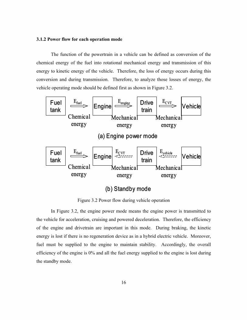
The photos, taken at ANL where the initial experiments were carried out, are
shown in Figure 4.8 and the facilities are summarized in Table 4.4. The fuel
consumption was obtained using both the fuel consumption meter and air flow meter
together with an air/fuel ratio meter.
Figure 4.8 OPA testing at ANL
Table 4.4 Test facilities at ANL
Facility Maker Model Dynamometer Clayton Emission bench Pierburg AMA 2000
AMA 4000 AF ratio E-TAS λ sensor Intake air flowrate Sierra 600-L04 Fuel consumption meter
Pierburg
Data acquisition National Instrument SCXI-1100 SCXI-1126
The chassis dynamometer at the University of Texas is a water brake type
dynamometer. The inertia masses were not hooked up to the dynamometer. Therefore,
only steady state tests were possible with this dynamometer. The fuel consumption rate
was measured using an AVL fuel consumption meter. The available facilities at UT are
29

summarized in the following Table 4.5. The OPA on the chassis dynamometer at UT is
shown in Figure 4.9.
The dynamometer settings used for the FTP test are as follows.
Test inertia: 3125 lbs
Road load:
)/(02055.0
)(93.382
2
0
220
mphlbff
lbffwherevffF
=
=⋅+=
Figure 4.9 OPA testing in UT
30

Table 4.5 Test facilities at UT
Facility Maker Model Specification/Remarks Dynamometer Clayton CT-200 Water brake type
Capacity: 200 hp Fuel consumption meter
AVL 730 Dynamic
Accuracy: 0.12% of consumed mass Measuring frequency: 1 Hz
CLA 53 NO/NOx analyzer Measuring range : 0–10~5,000 ppm Repeatability: ±1% of full scale Linearity: ±1% of full scale
Horiba
FIA-34A-2
HC analyzer Measuring range : 0–10~30,000 ppm HC Range: 0-10000 ppm vol.
Repeatability: within 1/3 of (±12ppm or ±5 % of readout)
CO Range: 0-10 % Repeatability: within 1/3 of (±0.06 % or ±5 % of readout)
Emissions bench
Horiba MEXA-554J
CO2 0-20 % Repeatability: within 1/3 of (±0.5 % or ±5 % of readout)
Data acquisition system
Fluke 2640 NetDAQ
Measurement: DC, AC, Resistance, Frequency, Thermocouple Channel: 20 ea Scan speed: Slow: 6 channels/sec Medium: 48 channels/sec Fast: 100 channels/sec
A/F ratio sensor
Horiba MEXA-110λ
Range: 0.0-99.9 (with gasoline) Within ± 0.1 A/F (at stoichiometry)
31

CHAPTER 5: FTP TEST RESULTS
The main reason for investigating a DISI engine is the benefit in fuel economy
and the barrier is strict emissions regulations in the U.S. The OPA with Toyota’s 2nd
generation D-4 engine and super CVT was tested for fuel economy and emissions on the
Federal Test Procedure. The measured fuel economy and emissions are compared with
those of the vehicle with the 1st generation D-4 engine. UT has already completed a
project of testing the Corona Premio which employs the previous version of Toyota’s
DISI engine in 1999. The Corona test data used for comparison are based on several
references [35] [37].
Selected topics and comparison issues are addressed in this section. Air/fuel ratio
control for the OPA is compared to that for the Corona in the following section. Fuel
economy and emissions are discussed in Sections 5.2 and 5.3 respectively. Additional
FTP results are provided in Appendix A.
5.1 AIR/FUEL RATIO CONTROL
Figure 5.1 shows the air/fuel ratio histories for the OPA and Corona during the
FTP cycle. Both the OPA and Corona begin the cycle with stoichiometric combustion
and, after a while, lean combustion starts. The onset of lean combustion for the Corona
was 256 seconds whereas that for the OPA is 416~529 seconds after vehicle start-up.
The main factor on this timing is the catalyst light-off. The temperatures of the
exhaust gas and catalysts are shown in Figure 5.2. For the Corona, only the exhaust
temperature is available so the catalyst temperature is plotted only for the OPA. The
exhaust temperatures of both vehicles are similar to each other as long as the combustion
control scheme is the same as each other, about 250 seconds after start-up. After that, the
exhaust temperature of the OPA is about 20~30 °C higher than that of the Corona
because its combustion remains stoichiometric.
32

Vehi
cle
spee
d (m
ph)
0
20
40
60
Phase 1 and 2 Phase 3
Air
fuel
ratio
10
20
30Corona
Lean onset: 256 sec
Air f
uel r
atio
10
20
30
Time (sec)
0 200 400 600 800 1000 1200 1400
Run 1 Run 2 Run 3
OPALean onset
529 sec416 sec470 sec
Time (sec)
0 100 200 300 400 500
Figure 5.1 Comparison of air/fuel ratio control
The catalyst is heated by hot exhaust gas and reaction heat within the catalyst.
The onset of lean combustion might be dependent on the temperature of the rear catalyst
because it is used to convert NOx emissions. The front catalyst temperature passes
500°C at 32 seconds and the rear catalyst passes at 259 seconds. Therefore, it is
reasonable to program the engine to begin the lean combustion at around 250 seconds. It
is not clear why the onset of the lean combustion is after 400 seconds for the OPA.
Veh
icle
spe
ed(m
ph)
0
20
40
60
Cat
alys
t tem
p (C
)
0200
400600
800
1000
Time(s)0 100 200 300 400 500
Front catalyst(OPA) Rear catalyst (OPA)
Exh
aust
tem
p. (C
)
0
200
400
600
800 OPA Corona
33Figure 5.2 Temperatures of the exhaust gas and catalysts

The D-4 engine is supposed to work in the lean combustion mode after catalyst
light-off. During lean combustion, the tailpipe NOx emissions are reduced by a NOx
storage reduction catalyst [17]. The mechanism is that NOx is stored and held in the
catalyst as nitrate at lean air/fuel ratios, then desorbed from the catalyst and reduced to
nitrogen using the reduction agent exhausted during stoichiometric combustion.
Therefore, the regular repetition of stoichiometric combustion is necessary. Figure 5.3
shows this operation during steady state and transient running of the vehicle. At constant
speed running as shown in Figure 5.3(a), the air/fuel ratio is kept constant and the rich
spikes occur periodically. At this rich spike, the throttle valve closes to reduce the
amount of air with the constant accelerator position. During the transient operation
shown in Figure 5.3(b), the stoichiometric combustions are seen for both the high load
and rich spikes for NOx regeneration.
Accel. position Throttle position
Time (sec)
150 200 250 300 350
Veh
icle
spe
ed (m
ph)
0
20
40
60
Air
fuel
ratio
0
10
20
30
40
Acc
el. p
ositi
on
Thro
ttle
posi
tion
0
1
2
3
4
Time (sec)
1100 1150 1200 1250 1300
(a) Steady state operation (b) Transient operation
Figure 5.3 Engine operation for NOx regeneration
34

Figure 5.4 shows the comparison between the OPA and Corona for the engine
operation, air/fuel ratio and engine speed. Even though the air/fuel ratio is transient and
complex, the range of air/fuel ratio for the OPA and Corona is similar to each other. The
air/fuel ratio during the idle for the OPA is 32 whereas that for the Corona is 27. The
engine speed of the OPA is controlled lower than that of the Corona due to the use of a
CVT.
Veh
icle
spe
ed (m
ph)
0
20
40
60
AF ra
tio
10
20
30
AF ratio at idle
OPA Corona
3227
Eng
ine
spee
d (r
pm)
0
500
1000
1500
2000
2500
Time (sec)
0 60 120 180 240 300
Figure 5.4 Comparison of engine operation for the OPA and Corona.
5.2 FUEL ECONOMY
The OPA was tested 3 times on the FTP cycle. The fuel economy results are
shown in Table 5.1 along with the fuel economy of the Corona. The Corona was the first
Toyota vehicle with the 1st generation D-4 engine. UT has conducted experiments on this
vehicle and presented the fuel economy and emissions results and examined the potential
of the DISI engine [36]. The FTP fuel economy of the OPA is 30.5 mpg, 10% less than
that of the Corona. There are two possibilities for this unexpected finding. One 35

possibility is that there is an actual difference in fuel economy and the other one is the
test variation. The weight of the OPA is 50 kg heavier than the Corona and the OPA is a
station wagon while the Corona is a sedan and thus should have a higher drag coefficient.
The specifications can affect the fuel economy difference. The test-to-test variation in
fuel economy for tests performed at the same lab is usually said to be 3%. However, the
OPA was tested on a chassis dynamometer at SwRI and the Corona was tested at GM.
The test-to-test variation together with the lab-to-lab variation can result in a 10%
difference in fuel economy. Therefore, it can not be stated with certainty that the fuel
economy of the OPA is 10% less than that of the Corona.
Table 5.1 Fuel economy of the OPA and Corona (mpg) [37]
Phase 1 Phase 2 Phase 3 Weighted resultsRun 1 25.812 31.876 34.877 31.079 Run 2 25.597 31.213 34.341 30.575 Run 3 24.968 30.535 33.444 29.804
Average 25.453 31.208 34.221 30.486 Corona 33.495
The fuel flowrate during the FTP cycle is shown in Figure 5.5. There is a small
difference in fuel consumption rate. In fact, the fuel economy data in the above table is
obtained from the CO2 concentration bag measurements and the fuel consumption rate in
Figure 5.5 is obtained from the instantaneous modal CO2 concentration and exhaust gas
flowrate. There is usually a discrepancy between the modal data and bag data. That is
the reason that the fuel consumption rates in Figure 5.5 do not show a big difference.
Anyway, what we can see from the fuel flowrate is that the fuel consumption patterns of
the OPA and Corona are similar to each other.
36

Veh
icle
spe
ed(m
ph)
0
20
40
60Fu
el ra
te (g
/sec
)
0.0
0.5
1.0
1.5
2.0
2.5
3.0 OPA Corona
Phase 1
Time (sec)
500 700 900 1100 1300
OPA Corona
Phase 2
Fuel
rate
(g/s
ec)
0.0
0.5
1.0
1.5
2.0
2.5
3.0
Time (sec)
0 100 200 300 400 500
Phase 3
Figure 5.5 Fuel flowrate during FTP cycle
5.3 EMISSIONS
The tailpipe emissions from the OPA on the FTP cycle are summarized in Table
5.2. The comparison of these emissions with the previous version D4 engine is shown in
Figure 5.6, which also shows the regulated levels. For this comparison, two sets of
standards were used. The first set is the intermediate useful life (50 kmile) Low Emission
Vehicle (LEV) standards fro the National Low Emission Vehicle (NLEV) program. The
FTP emissions are also compared to the intermediate life Tier 2 bins, which is effective
for 2004~2009 MY. Specifically, the emissions of the OPA are compared with Bin 10.
Regulators recognize the fact that some HC species are more ozone-forming than others.
Methane is essentially non-reactive and excluded from most regulations. Thus,
California hydrocarbon emissions are regulated in terms of Non-Methane Organic Gas
(NMOG) and Federal HC emissions as Non-Methane Hydrocarbons (NMHC). To
37

compare the measured emissions results with the emissions regulations, it is necessary to
convert the amount of THC into the terms actually used in the regulations. In this
research, the measured THC is converted into the NMOG using the factors suggested by
Lindhjem [27].
Table 5.2 FTP emissions test results for the OPA (unit: g/mile)
Phase 1
Phase 2 THC NOx CO CO2
THC NOx CO CO2 0.480 0.167 3.141 338.15
0.049 0.224 0.613 277.52
Phase 3
Weighted average THC NOx CO CO2
THC NOx CO CO2 0.056 0.342 0.531 258.90
0.141 0.245 1.114 283.52
As seen in Figure 5.6, the OPA meets only the CO standard for both regulations.
The NOx of the OPA meets Bin 10 of the Tier 2 EPA Bins but still needs improvement to
meet Bin 9, or LEV in the NLEV program. For the NMOG, the barrier is larger than for
the NOx. Although the D-4 engine is not calibrated for U.S. standards, this result implies
that the barriers for the DISI engine in the U.S. market are NOx and HC emissions, even
though Toyota has made considerable improvements to both with their second generation
D-4.
For all species except for carbon monoxide (CO), the tailpipe emissions of the
OPA are smaller than those of the Corona. The weighted average NMOG emissions
from the OPA are 30% less than that from the Corona. The NOx emissions of the OPA
are almost half of that from the previous D-4 vehicle. Even though the CO emissions
increase, its level is still below the regulated amount. Therefore, we can see that there is
a significant improvement in the development of the 2nd generation D-4 engine. The
following is a detailed analysis about the sources of these improvements.
38

0.0
0.2
0.4
0.6
0.8
1.0
1.2
NMOG NOx CO
Tailp
ipe F
TP e
mis
sio
n (
g/m
ile)
Corona OPA
-30%
-49%
+67%
NLEV 50K LEV CO standards: 3.4 g/mile
TIER 2 BIN 10 at 50K
0.0
0.2
0.4
0.6
0.8
1.0
1.2
NMOG NOx CO
Tailp
ipe F
TP e
mis
sio
n (
g/m
ile)
Corona OPA
-30%
-49%
+67%
NLEV 50K LEV CO standards: 3.4 g/mile
TIER 2 BIN 10 at 50K
Figure 5.6 Comparison of tailpipe emissions
5.3.1 THC emissions
The reason for the difference in emissions can be considered in two ways, engine-
out and after-treatment. To make this reason clear, the engine-out and tailpipe THC and
catalyst efficiencies are shown in Figure 5.7. The difference in the amount of engine-out
THC appears in the same quantitative way. The catalyst efficiencies are almost the same
as each other. The change in combustion system using slit nozzle injector seems to be
effective for the reduction of engine-out HC. According to Toyota [18], [23], the fuel
spray from the slit nozzle injector can be mixed well with air more evenly than the
previous cone spray and the reduced under-mixing and over-mixing can effectively
reduce HC emissions.
39

0
20
40
60
80
Phase 1 Phase 2 Phase 3 Total
Mas
s em
issi
on (g
)
OPA Corona
0.0
1.0
2.0
3.0
Phase 1 Phase 2 Phase 3 Total
Mas
s em
issi
on (g
)
OPA Corona
70%
80%
90%
100%
Phase 1 Phase 2 Phase 3 Total
Effic
ienc
y (%
)
OPA Corona
(a) Engine-out emissions (b) Tailpipe emissions (c) Catalyst efficiency
Figure 5.7 Source of THC difference between the OPA and Corona
Figure 5.8 shows the second by second HC emissions for Phases 1~3 of the FTP
cycle. It is seen in this figure that the OPA emits less HC than the Corona except for the
initial period until 250 seconds while both engines are working in a stoichiometric
combustion mode.
HC
(g/s
ec)
0.00
0.03
0.06
0.09
0.12 OPA Corona
Phase 1
Time (sec)500 700 900 1100 1300
Phase 2
HC
(g/s
ec)
0.00
0.03
0.06
0.09
0.12
Time (sec)0 100 200 300 400 500
Phase 3
Vehi
cle
spee
d(m
ph)
0
20
40
60
Figure 5.8 Comparison of engine-out THC between the OPA and Corona during the FTP
cycle
40

5.3.2 NOx emission
The reasons for decreased NOx emissions are investigated in the same way as for
THC. The engine-out and tailpipe NOx and catalyst efficiencies are shown in Figure 5.9
to see which factor dominates the reduced tailpipe NOx emissions. The dominant factor
seems to be different from that for THC. In the case of THC, the catalyst efficiency is
similar to each other and the decrease in engine-out emissions is the reason for the
decreased tailpipe emission. In contrast, the engine-out NOx emissions for the OPA are
more than that of the Corona but the tailpipe emissions are less than the Corona. This
means that the catalyst plays a significant role in the reduction of tailpipe emissions in the
case of NOx. As shown in Figure 5.9(c), the NOx purification efficiency of the catalyst
of the OPA is far better than that of the Corona in every phase of the FTP cycle. Toyota
increased the capacity of the NOx absorption reduction catalyst by 1.5 times compared to
the previous version and used a lot more EGR to decrease the engine-out NOx emissions.
From this result, it can be concluded that the improvement in after-treatment is more
effective than the changes to the combustion process (EGR).
0
10
20
30
Phase 1 Phase 2 Phase 3 Total
Mas
s em
issi
on (g
)
OPA Corona
0
2
4
6
Phase 1 Phase 2 Phase 3 Total
Mas
s em
issi
on (g
)
OPA Corona
0%
20%
40%
60%
80%
100%
Phase 1 Phase 2 Phase 3 Total
Effic
ienc
y (%
)
OPA Corona
(a) Engine-out emissions (b) Tailpipe emissions (c) Catalyst efficiency
Figure 5.9 Source of NOx difference between the OPA and Corona
Figure 5.10 shows the NOx conversion efficiency of the catalyst during the FTP
cycle. As the catalyst repeats absorption and regeneration during the transient operation,
the second by second conversion efficiency does not give the insight for the actual
41

conversion efficiency. Therefore, the efficiency is calculated within the interval between
the stoichiometric combustions as shown in the lower right graph of Figure 5.10.
Time (sec)500 700 900 1100 1300
Phase 2
Effic
ienc
y (%
)
0
20
40
60
80
100
Phase 3
OPA Corona
Effic
ienc
y (%
)
0
20
40
60
80
100
Time (sec)0 100 200 300 400 500
Phase 1
Veh
icle
spe
ed(m
ph)
0
20
40
60
AF ra
tio
10
20
30
Time (sec)
340 360 380 400 420 440 460 480
Interval
Figure 5.10 Comparison of NOx conversion efficiencies between the OPA and Corona
during the FTP cycle. The interval during which the efficiency is calculated is also illustrated.
Except for the initial 250 seconds before the catalyst light-off, the catalyst of the
OPA is more efficient than that of the Corona. For the latter part of Phase 1, the
difference is caused by the combustion scheme. The efficiency of the OPA is almost
100% because it is working in stoichiometric mode whereas the Corona is in lean
combustion mode. For Phases 2 and 3, where both vehicles are in the lean combustion
mode, the efficiency of the OPA catalyst is better than that of the Corona. Especially for
Phase 3, the difference in efficiency is larger than that for Phase 2. The engine load in
Phase 3 is larger than that of Phase 2 because the average vehicle speed is higher.
Therefore, the capacity of the Corona seems to be insufficient to purify the engine-out
NOx. That is why the efficiencies of the OPA for Phases 1~3 are similar to each other
but the efficiencies of the Corona for the 3 Phases are different from each other. For the
42

Corona, the efficiency during Phase 3 is worst and only 47.3% whereas that of the OPA
is 84.8%. The overall efficiency of the OPA is 89.9% and that of the Corona is 67.5%.
5.3.2 CO emissions
For the analysis of the increased tailpipe CO emissions, the engine-out and
tailpipe CO and catalyst efficiencies are shown in Figure 5.11. Both the engine-out and
tailpipe CO of the OPA are more than that of Corona. The catalyst efficiency of the OPA
is worse than those of the Corona. Every factor contributes to the increase in CO
emissions. However, the CO emissions are still within the regulated level even in the
strict U.S. standards.
0
20
40
60
80
100
120
140
Phase 1 Phase 2 Phase 3 Total
Mas
s em
issi
on (g
)
OPA Corona
0
3
6
9
12
15
Phase 1 Phase 2 Phase 3 Total
Mas
s em
issi
on (g
)
OPA Corona
70%
80%
90%
100%
Phase 1 Phase 2 Phase 3 Total
Effic
ienc
y (%
)
OPA Corona
(a) Engine-out emissions (b) Tailpipe emissions (c) Catalyst efficiency
Figure 5.11 Source of CO difference between the OPA and Corona
5.3 CHAPTER SUMMARY
The OPA was driven on the chassis dynamometer following the FTP cycle. The
operations of the OPA are compared with those of the Corona. The fuel economy and
emissions were measured and compared with those of the Corona. The factors affecting
the fuel economy and emissions were analyzed.
43

Both the OPA and Corona begin the FTP cycle with stoichiometric combustion
and, after a while, lean combustion starts and lasts until the end of the FTP. For the OPA,
the onset of lean combustion was 416~529 seconds after vehicle start-up. This onset
timing is delayed compared with that of the Corona. The fuel economy of the OPA is
30.5 mpg, 10% less than that of the Corona. This is because the vehicle resistance of the
OPA is larger than that of the Corona.
Toyota has made considerable improvements in tailpipe HC and NOx emissions
with their second generation D-4. For the HC emissions, the change in combustion
system using their slit nozzle injector seems to be effective. It was reported by Toyota
that the fuel spray from the slit nozzle injector can be mixed well with air more evenly
than the previous cone spray. In contrast, the dominant factor for the NOx reduction
turns out to be the catalyst efficiency. Due to the increase in the capacity of the catalyst,
the average catalyst efficiency for NOx is improved from 67.5% for the Corona to 89.9%
for the OPA.
Even with these improvements, the barrier of the U.S. market seems to remain
high for the DISI engine. The tailpipe NMOG and NOx do not meet the LEV standards
in the NLEV program.
44

CHAPTER 6: STEADY STATE RESULTS
Chapter 6 describes the steady state test results. The purpose of these steady state
tests was to examine the feasibility of an in-situ mapping technique and obtain the map
data for the OPA’s DISI engine and CVT. The in-situ mapping technique is a method of
getting map data in the actual vehicle on the chassis dynamometer instead of via engine
dynamometer testing. The key problem in this method is how to get the engine torque
with the engine in the vehicle. The installation of torque sensors at the output shafts of
the engine and CVT was developed and used. Part of this experiment was done with both
torque sensors and the remaining part was done with only the axle torque sensor. In the
latter case, the efficiency map of the CVT, which was obtained from the previous tests
with both torque sensors, was used to estimate the engine torque.
The measured map plots of steady state results are presented in Appendix B.
Some of the important issues are selected and addressed in the following sections.
6.1 STEADY STATE VEHICLE OPERATION
The emissions were measured at constant vehicle speed under road load
conditions and the measured results are shown in Figure 6.1. The air/fuel ratio is
controlled at around 30 at 20 mph and decreases as the vehicle speed increases. In this
figure, two kinds of rich spikes are observed. The air/fuel ratio goes down to near
stoichiometry when the vehicle is accelerated because the engine load goes beyond the
lean combustion region. The other kind of spikes occurs regularly to regenerate the NOx
catalyst.
Every species, both engine-out and tailpipe, change according to the change in
load and air/fuel ratio. The behaviors of both HC and CO concentrations are directly
linked to the air/fuel ratio. Their peaks coincide with the rich spikes. Similar trends can
be seen in the NOx concentration. During lean combustion, the engine-out NOx remains
constant but the tailpipe NOx concentration increases gradually. This indicates that the
45

catalyst efficiency decreases with time as the NOx is absorbed in the catalyst until the
next regeneration occurs to purge the absorbed NOx and increases the efficiency again. V
ehic
le s
peed
(mph
)
0
20
40
HC
Con
cent
ratio
n (p
pmC
)
0
2000
4000
6000
8000 Engine-out Tailpepe X 5
CO
Con
cent
ratio
n (%
)
0
1
2
3
4
Time (sec)
0 50 100 150 200 250 300 350
Engine-out Tailpipe
NO
x C
once
ntra
tion
(ppm
)
0
300
600
900 Engine-out Tailpipe
AF ra
tio
10
20
30
Rich spike for NOx regeneration
Rich spike at high acceleration
Figure 6.1 Emissions during steady state engine operation
46

6.2 CVT EFFICIENCY
The fuel consumption and emissions of the engine and the efficiency of the CVT
were obtained using the in-situ mapping technique. The torque sensors between the
engine and the CVT and those between the CVT and wheels enable the measurement of
the CVT efficiency. The efficiency of the CVT is defined as the ratio of the output power
to the input power as shown in the following equation. Table 6.1 shows the physical
quantities in this equation.
engineengine
axleaxleCVT powerEngine
powerAxleωτωτη
××
== (6.1)
Table 6.1 Measured physical quantities used to calculate the CVT efficiency
Power Formulae Physical quantity Measurement Torque Engine torque sensor
(HBM T10F) Engine power engineengine ωτ ×
Speed CPS(Crank Position Sensor) signal Torque Two torque sensors, one on each
axle shaft Axle power axleaxle ϖτ ×
Speed CVT output speed signal
For the measurement of fuel consumption and emissions, the engine torque sensor
was used while the chassis dynamometer absorbs the power of the engine as if the engine
is mounted on the engine dynamometer. A part of this experiment was done with both
torque sensors and the other part was done without the engine torque sensor because the
engine torque sensor got out of order. For the latter part of this experiment, the efficiency
of the CVT was used to estimate the engine torque from the axle torques.
Figure 6.2 shows the measured efficiency of the CVT. The losses in the CVT are
composed of oil pump power, belt drag and frictional losses in the gears and bearings
[22]. In Figure 6.1, it is seen that the input engine torque, expressed as BMEP, is the
dominant factor and engine speed and gear ratio also affect the efficiency of the CVT.
As the input torque increases, the efficiency increases and as the engine speed increases,
47

the efficiency decreases. At the same engine speed and torque, the efficiency at middle
ratio with the similar radius of belt pulley is better than that of high or low ratio.
Engine speed (rpm)
500 1500 2500 3500 4500 5500
0.65 0.65 0.65
0.76 0.76 0.76
0.82 0.82 0.82
0.85 0.85 0.85
0.880.88
0.880.90
0.90
BM
EP (b
ar)
1
3
5
7
9
11
Engine speed (rpm)
500 1500 2500 3500 4500 5500
0.74 0.74 0.74
0.830.83 0.83
0.870.87
0.870.90
0.900.90
0.920.92
0.920.930.93
(a) At middle ratio ( 1≈out
in
ωω ) (b) At high or low ratio
Figure 6.2 Efficiencies of the CVT
Direct measurement of the engine torque is the best way for the engine map test
but an indirect method was used due to the problems with the engine torque sensor. To
check the validity of this approach, the errors of engine torque were estimated from the
measured torque, as shown in Figure 6.3. The actual torques directly measured from the
engine torque sensor are compared with those estimated from the axle shaft torque and
rotational speed on both sides of the CVT using the efficiency map in Figure 6.3. The
frequency of the error at each range is counted and shown in this figure for the 43
measurement points. The maximum error is 1.6 N-m and more than 90% of the
measurements are within 1 N-m.
48
-2 -1 0 1 20
2
4
6
Error (Nm)
frequency
Figure 6.3 Estimated error in engine torque calculation
The CVT efficiency map was used to estimate the engine torque for both engine
map testing and simulation. From the results in Figure 6.3, it appears that this method for
engine torque estimation is reliable even though it is not measured directly.
6.3 AIR/FUEL RATIO DISTRIBUTION
As the in-situ mapping test was done in an actual vehicle, the operation is
different from testing on an engine dynamometer. It was not possible to locate the
operating point on the exact point of pre-selected engine speed and torque. The operating
point was controlled as close to the target as possible by manipulating the throttle pedal
and the load of the chassis dynamometer.
Experiments were done in both the lean and stoichiometric combustion mode.
The operating points are shown in Figure 6.4 for normal operating conditions. The
markers indicated as stoichiometric mean that the operating points go beyond the lean
combustion range.
49
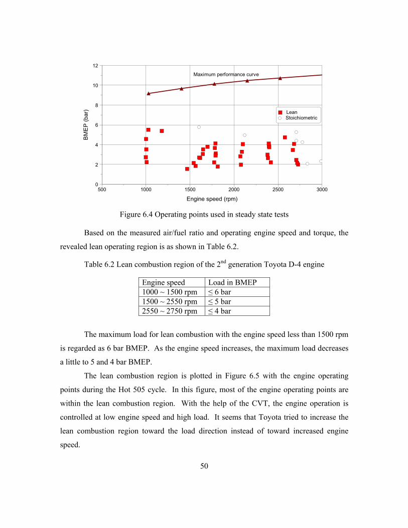
BM
EP
(bar
)
0
2
4
6
8
10
12
Engine speed (rpm)500 1000 1500 2000 2500 3000
Lean Stoichiometric
Maximum performance curve
Figure 6.4 Operating points used in steady state tests
Based on the measured air/fuel ratio and operating engine speed and torque, the
revealed lean operating region is as shown in Table 6.2.
Table 6.2 Lean combustion region of the 2nd generation Toyota D-4 engine
Engine speed Load in BMEP 1000 ~ 1500 rpm ≤ 6 bar 1500 ~ 2550 rpm ≤ 5 bar 2550 ~ 2750 rpm ≤ 4 bar
The maximum load for lean combustion with the engine speed less than 1500 rpm
is regarded as 6 bar BMEP. As the engine speed increases, the maximum load decreases
a little to 5 and 4 bar BMEP.
The lean combustion region is plotted in Figure 6.5 with the engine operating
points during the Hot 505 cycle. In this figure, most of the engine operating points are
within the lean combustion region. With the help of the CVT, the engine operation is
controlled at low engine speed and high load. It seems that Toyota tried to increase the
lean combustion region toward the load direction instead of toward increased engine
speed.
50

BM
EP
(bar
)
0
2
4
6
8
10
12
Engine speed (rpm)500 1500 2500 3500 4500 5500
Maximum performance curve
Lean combustion region
BM
EP
(bar
)
0
2
4
6
8
10
12
Engine speed (rpm)500 1500 2500 3500 4500 5500
Engine operating pointsduring HOT 505 cycle
Figure 6.5 Measured lean combustion region
The air/fuel ratio distribution is shown in Figure 6.6. At low engine speed and
low load, the air/fuel ratio is controlled high and decreases as the engine speed and load
increase. In the manual for the OPA published by Toyota, it is stated that the maximum
air/fuel ratio is 50. However, in these experiments, the measured maximum air/fuel ratio
was 30 as shown as a marker in Figure 6.6.
BMEP
(bar
)
1
2
3
4
5
6
Engine speed (rpm)
1000 1500 2000 2500 3000
15
15
15
21
2121
24
24
24
24
2426
26
Measured maximumair fuel ratio (30)
Figure 6.6 Air/fuel ratio distribution
51

6.4 FUEL CONSUMPTION
The measured brake specific fuel consumption maps, in g/kW-hr, for both the
lean and stoichiometric combustion modes are shown in Figure 6.7. The fuel
consumption rate used to calculate the BSFC in this figure is the average fuel
consumption rate for at least 2 minutes. Therefore, the fuel consumption includes the
effect of fuel enrichment for NOx regeneration. As the load increases, the specific fuel
consumption decreases monotonically in the stoichiometric combustion mode. In
contrast, the specific fuel consumption for the lean combustion mode decreases rapidly at
low load and then the rate of decrease becomes small.
Lean combustion
BMEP
(bar
)
0
2
4
6
8
10
12
Engine speed (rpm)
500 1000 1500 2000 2500 3000
265
265265
265
294294
294294
270
270
270
270280
280
280
280280280
320320320
Leanoperation region
Maximum performance
Stoichiometric combustion
Engine speed (rpm)
500 1000 1500 2000 2500 3000
265
265 265
300300300
270
270
270
270
320320320
370370370
340 340 340
Maximum performance
(a) Map
BSF
C (g
/kw
-hr)
260
300
340
380
420
BMEP (bar)
1 2 3 4 5 6
Lean Stoichiometric
14 %
1200 rpm
19 %
BMEP (bar)
1 2 3 4 5 6
1800 rpm
12 %
16 %
(b) Plots at 1200 rpm and 1800 rpm
52Figure 6.7 Brake specific fuel consumption of the 2nd generation D4 engine

Figure 6.8 shows the relative SFC decrease in lean combustion mode compared to
the SFC in stoichiometric combustion mode. Within the lean operation region, the
improvement in fuel consumption is best at low engine speed and 3 bar BMEP. From
this figure, the fuel consumption improvement at low speed and 2~4 bar is about 20%.
Figure 6.8 Relative improvement in SFC (
tricstoichiome
tricstoichiomelean
sfcsfcsfc −
×= 100 )
6.5 EMISSIONS
The emission rates are expressed in terms of BSHC(Brake Specific HC) and
BSNOx(Brake specific NOx). The definitions are as followings.
(( )
)(:/:
/:
kWpowerbrakebphrgNOxofflowratemassm
hrgHCofflowratemassmWherebp
mhrkW
gBSNOx
bpm
hrkWgBSHC
NOx
HC
NOx
HC
&
&
&
&
=
⋅
=
⋅
) (6.2)
53

The change in BSHC and BSNOx according to the load at 1200 and 1800 rpm are
shown in Figure 6.9. BSHC in lean combustion is 2~3 times of that in the stoichiometric
combustion mode. On the other hand, the lean BSNOx is about one-half to one sixth
compared to that in the stoichiometric combustion mode.
1200 rpm 1800 rpm
BSH
C (g
/kw
-hr)
0
2
4
6
8
10
BMEP (bar)
2 3 4 5
Lean Stoichiometry
BMEP (bar)
2 3 4 5
(a) BSHC (g/kW-hr)
1200 rpm 1800 rpm
BS
NO
x (g
/kw
-hr)
0
5
10
15
20
BMEP (bar)2 3 4 5
Lean Stoichiometry
BMEP (bar)2 3 4 5
(a) BSNOx (g/kW-hr)
Figure 6.9 Steady state emissions
The FTP test results for the 1st generation D-4 of Toyota were reported by Chad
and coworkers [36] and those for the Mitsubish Legnum with a 1.8L GDI engine were
reported by Cole and coworkers [8]. They compared the engine-out and tailpipe
emissions with those of comparable PFI(Port Fuel Injection) engine. According to the
results of Chad and coworkers [36], the difficulties for the HC emissions are the engine-
out HC emissions for all modes of operation during the FTP cycle. Those for the NOx
emissions stem from the low efficiency of the lean NOx catalyst in the DISI vehicle. The 54

rich and lean ends of the gradient in the DISI engine working under stratified charge
mode give rise to unburned HC. Another source is wall wetting on the piston and
cylinder liner. These are the cause of increased HC in DISI engine.
The NOx emissions decrease as the load increases in the lean mode whereas that
in the stoichiometry mode increases. This is because the usage of EGR is different for
lean stoichiometric operation. The stock ECU does not control the EGR valve during
stoichiometric operation. In contrast, during the lean combustion mode, the EGR rate
increases as the load increases as shown in Figure 6.10. Due to the restriction in facilities
at UT, the actual EGR ratio could not be measured and the EGR step number shown on
the scan tool was recorded and shown in Figure 6.10.
To compare the difference in emissions for the lean and stoichiometric
combustion modes, the emissions during the last 160 seconds in Phase 1 and 3 are shown
Figure 6.10. As the engine is warmed-up during this period, the only difference is the
air/fuel control scheme as shown in Figure 6.10(b). As expected from the measured
steady state emissions results, the engine-out HC in the lean mode is more than that in the
stoichiometric mode and the engine-out NOx in the lean mode is far less than that in the
stoichiometric mode.
EGR
ste
p nu
mbe
r
0
10
20
30
40
50
60
BMEP (bar)
1 2 3 4 5 6
BMEP (bar)
1 2 3 4 5 6
(a) 1200 rpm (b) 1800 rpm
Figure 6.10 Change in EGR step according to load 55

Veh
icle
spe
ed(m
ph)
0
20
40
60
NO
x (m
g/se
c)
0
20
40
60
80
100Engine-out Phase 1 Phase 3
NO
x (m
g/se
c)
0
3
6
9
12
Time (sec)
340 380 420 460 500
Tailpipe
HC
(mg/
sec)
0
20
40
60
80
100 Engine-out Phase 1 Phase 3
Phase 1 Phase 3
AF ra
tio
10
20
30
40 Phase 1 Phase 3
HC
(mg/
sec)
0
1
2
3
4
Time (sec)340 380 420 460 500
Tailpipe
Figure 6.11 Effect of combustion mode on the emissions during the last 140 seconds of
FTP Phase 1 and 3
6.6 IGNITION AND INJECTION TIMING
The strategies for ignition timing calibration are either MBT or retardation for
emissions reduction. Figure 6.12 shows the mapped ignition timing for the lean and
stoichiometric modes. Both ignition timings at 1200 rpm are similar to each other but
those in the lean burn mode are retarded by 5 ° compared to those in stoichiometric
combustion mode. This indicates that the burning speed in the lean stratified charge
mode is faster than that in homogeneous stoichiometric mode. Makato and coworkers
[18] who presented a paper regarding this D-4 engine claimed that the stratified
combustion has a short ignition delay and a large heat release at the beginning. It seems
that the mapped ignition timing in the lean combustion mode is close to the TDC as a
result of faster burning speed.
56

Igni
tion
timin
g (d
eg B
TDC
)
5
10
15
20
25
30
35
BMEP (bar)
1 2 3 4 5 6
1200 rpm Stoichiometry Lean
BMEP (bar)
1 2 3 4 5 6
1800 rpm
Figure 6.12 Comparison of ignition timing
The injection timing shown in Figure 6.13 is mostly dependent on the engine
speed. As the engine speed increases, the duration for mixture preparation in terms of
crank angle increases. The advance in injection timing with load is also observed.
Inje
ctio
n tim
ing
(deg
BTD
C)
40
50
60
70
80
Engine speed (rpm)
1000 1500 2000 2500 3000
3.5 bar BMEP 2.5 bar BMEP 4.5 bar BMEP
Load
Figure 6.13 Injection timing
57
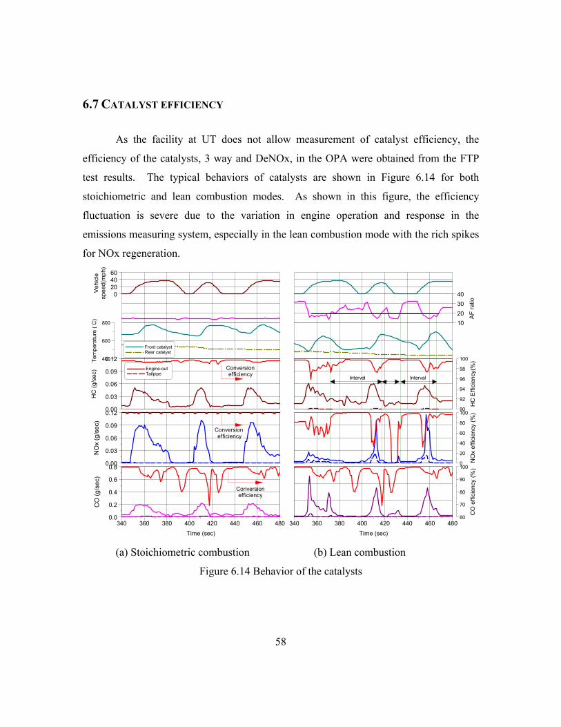
6.7 CATALYST EFFICIENCY
As the facility at UT does not allow measurement of catalyst efficiency, the
efficiency of the catalysts, 3 way and DeNOx, in the OPA were obtained from the FTP
test results. The typical behaviors of catalysts are shown in Figure 6.14 for both
stoichiometric and lean combustion modes. As shown in this figure, the efficiency
fluctuation is severe due to the variation in engine operation and response in the
emissions measuring system, especially in the lean combustion mode with the rich spikes
for NOx regeneration.
Time (sec)340 360 380 400 420 440 460 480
AF ra
tio
10203040
HC
Effi
cien
cy(%
)
90
92
94
96
98
100
Interval Interval
CO
effi
cien
cy (%
)
60
70
80
90
100N
Ox
effic
ienc
y (%
)0
20
40
60
80
100
Vehi
cle
spee
d(m
ph)
0204060
CO
(g/s
ec)
0.0
0.2
0.4
0.6
0.8
Time (sec)340 360 380 400 420 440 460 480
HC
(g/s
ec)
0.00
0.03
0.06
0.09
0.12 Engine-out Tailpipe
NO
x (g
/sec
)
0.00
0.03
0.06
0.09
0.12
Conversionefficiency
Conversion efficiency
Conversionefficiency
Tem
pera
ture
( C
)
400
600
800
Front catalyst Rear catalyst
(a) Stoichiometric combustion (b) Lean combustion
Figure 6.14 Behavior of the catalysts
58
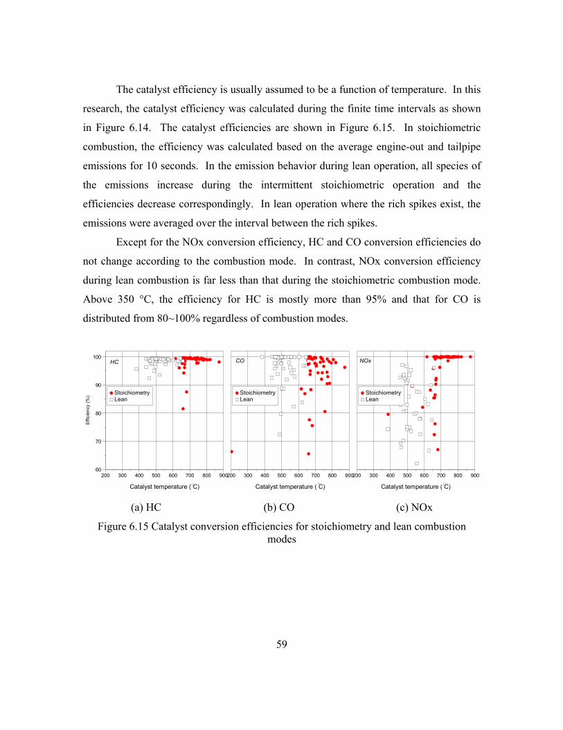
The catalyst efficiency is usually assumed to be a function of temperature. In this
research, the catalyst efficiency was calculated during the finite time intervals as shown
in Figure 6.14. The catalyst efficiencies are shown in Figure 6.15. In stoichiometric
combustion, the efficiency was calculated based on the average engine-out and tailpipe
emissions for 10 seconds. In the emission behavior during lean operation, all species of
the emissions increase during the intermittent stoichiometric operation and the
efficiencies decrease correspondingly. In lean operation where the rich spikes exist, the
emissions were averaged over the interval between the rich spikes.
Except for the NOx conversion efficiency, HC and CO conversion efficiencies do
not change according to the combustion mode. In contrast, NOx conversion efficiency
during lean combustion is far less than that during the stoichiometric combustion mode.
Above 350 °C, the efficiency for HC is mostly more than 95% and that for CO is
distributed from 80~100% regardless of combustion modes.
Catalyst temperature ( C)
200 300 400 500 600 700 800 900
CO
Stoichiometry Lean
Catalyst temperature ( C)
200 300 400 500 600 700 800 900
HC
Stoichiometry Lean
Effic
ienc
y (%
)
60
70
80
90
100
Catalyst temperature ( C)
200 300 400 500 600 700 800 900
NOx
Stoichiometry Lean
(a) HC (b) CO (c) NOx
Figure 6.15 Catalyst conversion efficiencies for stoichiometry and lean combustion modes
59

6.8 CHAPTER SUMMARY
The in-situ mapping technique turns out to be feasible to measure the map data for
the engine and transmission in case that the dynamometer test for the engine and
transmission itself is hard to perform. In this research, the steady state characteristics of
DISI engine and CVT in Toyota’s OPA was collected using the in-situ mapping
technique.
The operating range of the lean combustion control was revealed. The maximum
load for the lean combustion decreases as the engine speed increases and that for less
than 1500 rpm was 6 bar BMEP. The maximum engine speed for lean combustion was
found to be 2750 rpm. The mapped air/fuel ratio decreases as the engine speed and load
increases. The measured maximum air/fuel ratio was 30 at 1000 rpm and 2.3 bar BMEP.
The improvement in steady state fuel consumption is about 20% at low speed and
around 3 bar BMEP. This improvement decreases at lower and higher load and higher
engine speed. The engine-out HC emissions in terms of BSHC for the lean combustion
are 2~3 times of that in the stoichiometric combustion mode. The engine-out NOx
emissions are about one-half to one-sixth compared to that in the stoichiometric
combustion mode. It was confirmed again that the higher level of HC emissions in lean
combustion mode come from the engine-out emission and that of NOx emission stem
from the less efficiency of catalyst.
60

CHAPTER 7: OVERALL EFFICIENCY MEASUREMENTS
In order to determine the factors that affect fuel economy quantitatively, the
power flows through the major powertrain components were measured during operation
over transient cycles. The fuel consumption rate and torque and speed of the engine
output and axle shafts were measured to assess the power flows in a vehicle with a CVT.
The measured power flows were converted to the energy loss for each component to
obtain the efficiency. Tests were done for Phase 1 and Phase 3 of the FTP and for two
different CVT shift modes. The measured energy distributions were compared with those
from the ADVISOR simulation and to results from the PNGV study.
The baseline combustion mode was the stoichiometric mode. As most of this
experiment was done when the lean mode engine control was unstable, there was not
enough data for the normal operation of the D-4 engine. Therefore, the data were
obtained by manipulating the engine combustion mode to stoichiometric mode. The
normal combustion mode data was added later and compared with the stoichiometric
mode data.
The measured torque and speed are used to locate the operating point on the
efficiency map as well as to calculate the energy flows and losses. The measured powers
and calculated energy flows are plotted and related issues are discussed in the following
sections.
7.1 MEASURED TORQUE AND POWER
The engine torque and axle torque measured using the installed torque sensors are
shown in Figure 7.1 and Figure 7.2. Figure 7.1 shows the operating points during the Hot
505 cycle, based on the measured speeds and torques, superimposed on the engine’s
efficiency map.
In Figure 7.1, the engine efficiency map was obtained from the steady state
experiments with the same measurement system as explained in the previous chapter.
Fuel consumption rates at steady state were measured by changing gear ratio and vehicle
61

speed so that fuel consumption data would be obtained at several engine operating points.
From Figure 7.1, it can be seen that the CVT allows the engine to operate close to the
best efficiency line during much of the cycle. As noted previously, the test vehicle is
equipped with a CVT, for which a continuously variable gear ratio is available.
Figure 7.1 Engine operating points during the Hot 505 cycle.
Figure 7.2 shows the engine and axle torque changes as the vehicle accelerates
and decelerates. The two measured axle torques are not exactly in accord with each
other. It is seen that the engine torque is around 18 N⋅m and axle torques are around 100
N⋅m during idling. While decelerating, the engine torque becomes negative due to the
transmitted power from the vehicle’s inertia.
62

Figure 7.2 Measured engine and axle torques during the Hot 505 cycle
The power flows from the fuel through the powertrain to the vehicle can be
calculated from the measured fuel rate, torques and speeds. Figure 7.3(a) shows the
measured fuel energy addition rate (“fuel power”), engine power and axle power. The
cumulative energies are shown in Figure 7.3(b).
63

(a) Power flows
(b) Cumulative energy of each component
Figure 7.3 Measured power and energy during the Hot 505 cycle.
Figure 7.4 shows the instantaneous efficiency of the engine and drivetrain during
the engine power mode. As shown via the engine operating points on the efficiency map
in Figure 7.2, the efficiency of the engine varies between 0 (during deceleration) to 34%
over the Hot 505 cycle. However, as shown in Figure 7.4, during engine power mode
64

operation, the engine efficiency varies from 20~34% and the average engine efficiency is
29.3%.
Figure 7.4 Measured efficiencies of the engine and CVT during the Hot 505 cycle.
The efficiency of the CVT is low during the early stages of acceleration, when the
clutch is not yet locked up. It is seen in Figure 7.5 that the efficiency of the CVT does
not exceed 80% with the unlocked clutch, but once the clutch is locked-up the efficiency
goes beyond 80%. The measured CVT efficiency is in the range of 50~90% with an
average of 78.4% during power mode operation.
65

Figure 7.5 Change of the CVT efficiency according to the clutch state.
7.2 ENERGY LOSS DISTRIBUTION
The energy losses for each major component were calculated for the two
operating modes, engine power and standby, and are shown in Figure 7.6. In the Hot 505
cycle experiments, 12% of the fuel energy was consumed for idling and braking for this
test vehicle.
In Figure 7.6 it can be seen that the most energy was consumed by the engine.
The CVT loss was only 5.6% of total fuel consumption. The energy conversion
efficiency from fuel to engine-out mechanical energy is quite low compared to that of
mechanical power transmission via the CVT. Nevertheless, the efficiency of the
transmission is significant because a relatively small loss in the transmission can cause a
relatively larger energy loss in the engine due to the limited efficiency of the engine.
66

Engine loss(62.3% )
Road load+ Acceleration
20.2%
Stabilization11.8%
CVT loss5.6%
Engine power modeStandby mode
Engine loss(62.3% )
Road load+ Acceleration
20.2%
Stabilization11.8%
CVT loss5.6%
Engine power modeStandby mode
Figure 7.6 Energy loss distributions.
7.3 EFFECT OF ADDITIONAL PARAMETERS
In addition to the results shown above, more experiments were performed to
examine the effect of cold vs. warm start and of the shift mode and of the combustion
mode, as discussed below.
7.3.1 Effect of warm-up
In addition to the Hot 505 cycle, the Cold start 505 cycle (Phase 1 of the FTP)
was performed to quantify the effect of the powertrain warm-up on the energy
distribution. Based on the measured energy flow through each powertrain component,
the energy losses and efficiencies were calculated, as shown in Figure 7.7.
67

0
50
100
150
200
250
300
Engine CVT Vehicle Idle & Braking
Components
Fuel
loss (
g)
Hot 505 cycleCold 505 cycle
(a) Energy losses in terms of fuel consumption
0%
20%
40%
60%
80%
100%
Engine CVT
Components
Eff
icie
ncy (
%)
Hot 505 cycleCold 505 cycle
29.3%25.0%
78.4%74.1%
(b) Efficiencies of engine and CVT
Figure 7.7 Comparison of the energy loss and efficiency according to the warm-up
For cold starts, more fuel must be supplied to overcome the increased friction of
the engine and CVT and to compensate for incomplete vaporization of the fuel.
Moreover, the increased idle speed consumes more fuel. Thus, it is shown in Figure 7.7
that the energy losses for the cold start test are larger than those for the hot start test,
especially in the engine. The change in the average efficiency of the engine and CVT
68

was 4.3 percentage points for both, even though the effect on the engine was expected to
be larger than for the CVT.
Even though the average (over the cycle) efficiency changed by 4.3 percentage
points for both the engine and CVT for the hot vs. cold starts, the effect on the engine is
much more important because its baseline efficiency (29.3%) is much lower than for the
CVT (78.4%). That is, the 4.3% percentage point decrease in engine efficiency translates
to a 14.7% loss in efficiency, whereas the CVT experienced only a 5.5% loss in
efficiency. Of course, the product of the two efficiencies affects fuel economy.
Table 7.1 Fuel economies according to warm-up state
Operation Cold start Hot start Difference
Fuel economy (mpg) 24.27 32.99 8.72 mpg (26.4%)
As a result of this increased energy loss, the fuel economy deteriorated, as shown
in Table 7.1. About 36% more fuel was used to run the same distance with the same
driving schedule. This additional fuel input contributes to the worse fuel economy. From
the measured energy losses for each component, the factors which affect the change in
fuel economy were quantified, as shown in Figure 7.8. More than 93% of the decrease in
fuel economy for the cold start test can be attributed to the engine.
0
5
10
15
20
25
30
35
Fuel econom
y (m
pg)
Hot start
Engine
Idle and braking
CVT
Vehicle
0
5
10
15
20
25
30
35
Fuel econom
y (m
pg)
Hot start
Engine
Idle and braking
CVT
Vehicle
Cold startCold start
Figure 7.8 Change in fuel economy and contribution of each component 69

7.3.2 Effect of shift mode
The test vehicle in this research has two modes of gear shifting. One is the
normal mode, seeking fuel economy, and the other is a sports mode, seeking torque and
acceleration. In the sports mode, the engine operates mainly at high speed to realize a
high level of acceleration. However, as there is a trade-off between the power and fuel
economy, the sports mode is expected to increase fuel consumption. In this research,
with the measurement of the fuel consumption and efficiencies of the engine and CVT,
the effect of the shift mode was quantified.
The operating points of the engine and CVT on their efficiency maps are shown in
Figure 7.9. Both efficiency maps, of the engine and CVT, were obtained by measuring
the power flow in and out of the components at steady state. As shown in Figure 7.9, use
of the sports mode results in operation at higher engine speeds. In general, this results in
both the engine and CVT operating at lower efficiency on their respective efficiency
maps.
The fuel economies for both operations are shown in Table 7.2. Using the sports
mode rather than the normal mode decreases fuel economy by 28.2%, for the Hot 505
test.
Table 7.2 Fuel economies according to shift mode
Operation Normal mode Sports mode Difference
Fuel economy (mpg) 32.99 23.25 28.2%
In order to clarify the factors that dominate this fuel economy loss, the energy
losses for each component were calculated. The results are shown in Figure 7.10. The
additional fuel losses for the engine and CVT are;
• Engine: 81.3 grams
• CVT: 10.2 grams
70

(a) On engine efficiency map
(b) On CVT efficiency map
Figure 7.9 Operating points according to shift modes
A portion of the increased fuel consumption by the engine is, in fact, due to the
CVT. The increased fuel consumption by the engine is caused by the CVT in 2 ways.
• Change of engine operating points
• Increased energy requirement from decreased efficiency of the CVT
71

As the engine has a limited efficiency, the increase in energy requirement from
the transmission necessarily increases the energy loss in the engine. That is, even if the
engine operating points do not change, the engine energy loss would have increased.
0
50
100
150
200
250
300
Engine CVT Vehicle Idle & Braking
Components
Fuel
loss (
g)
Normal mode
Sports mode
Figure 7.10 Energy losses at each component
Figure 7.11 shows the change of efficiencies of the engine and CVT. The
efficiency of the engine decreases about 4 percentage points and that of the CVT
decreases about 10 percentage points.
0%
20%
40%
60%
80%
100%
Engine CVT
Components
Eff
icie
ncy (
%)
Normal modeSports mode
Figure 7.11 Change of efficiencies by shift modes
72
7.4 COMPARISON WITH SIMULATION
In the vehicle simulation, the most important parameters are energy flows
between the major powertrain components. The fuel consumption and emissions make
sense only if the input and output torque and speeds of the powertrain components are
defined correctly. In this section, the measured fuel rates and power flows are compared
with the simulation results.
PSAT and ADVISOR were used as the simulation tools for this purpose. Both of
them are programmed in MATLAB/Simulink. PSAT uses a forward facing modeling
approach and ADVISOR uses backward facing modeling. The backward facing
calculation begins with a required speed trace that the vehicle must meet. The model
calculates the necessary force at the wheels to move the vehicle as required. It then
works backwards through differential, transmission, clutch and finally the engine. In
contrast, the forward facing approach starts from the driver and determines the power
requirement based on the difference between the actual speed and target speed. Then,
this power transmits to the vehicle through the components such as the clutch,
transmission, final drive and wheel.
The calculations of power through each component are based on the efficiency
and performance of each component. Therefore, the required input includes the
efficiency maps for each powertrain component: engine, CVT, and so on. In this
research, those efficiency maps were generated by steady state mapping tests and used in
this simulation. For example, the efficiency of the engine was obtained by measuring the
torque and speed of the engine keeping the vehicle at constant speed. The basic model
parameters for this simulation are shown in Table 7.3.
Figure 7.12 shows the measured results and simulation predictions
simultaneously. From this figure, the simulated results agree well with the measured
results.
73

Table 7.3 Description of basic model parameters
Component Parameter Specification Source Frontal area 2.5848 m2 Specification Weight 1417.5 kg Specification Drag coefficient 0.3362 Vehicle Rolling resistance coefficient 0.009843 Coast down test
Max torque curve In Figure 6.7 (a) Specification Engine BSFC Map In Figure 6.7 (a) Steady state test Ratio range 0.428~2.396 Specification CVT Efficiency map In Figure 6.2 (b) Steady state test
From the simulated power flows, the energy losses for each component were
calculated, as shown in Figure 7.13(a). Comparing this result with the measured results
in Figure 7.6, we can see that the simulation makes a good estimation for the energy loss
of each component. As expected from Figure 7.12, the stabilization loss in the
ADVISOR simulation is a little larger than measured and that in the PSAT simulation is a
little less. The estimated loss contributions of the other components do not deviate more
than 4%.
74

Veh
icle
spe
ed(m
ph)
0
20
40
60
Eng
ine
spee
d (r
pm)
0
1000
2000
3000R
educ
tion
ratio
(-)
0.0
0.5
1.01.5
2.0
2.5
Time (sec)
0 100 200 300 400 500
Experiment ADVISOR simulation PSAT simulation
Eng
ine
torq
ue (N
m)
-50
0
50
100
150
(a) Engine speed and torque
Veh
icle
spe
ed(m
ph)
0
20
40
60
Pow
er (k
W)
-10
0
10
20
30
40
Experiment ADVISOR simulation PSAT simulation
Engine power
Pow
er (k
W)
-10
0
10
20
30
40
Time (sec)0 100 200 300 400 500
Axle power
Fuel
flow
rate
(g/s
ec)
0
1
2
3
(b) Power through the engine and CVT
Figure 7.12 Comparison of measured power flows with simulated 75

Engine loss(60.8%)
Road load+ Acceleration
19.2%
Stabilization14.6%
CVT loss5.4%
Engine power modeStandby mode
Engine loss(64.8%)
Stabilization7.8%
Road load+ Acceleration
21.1%
CVT loss6.6%
Engine power mode
Standby mode
Engine loss(60.8%)
Road load+ Acceleration
19.2%
Stabilization14.6%
CVT loss5.4%
Engine power modeStandby mode
Engine loss(64.8%)
Stabilization7.8%
Road load+ Acceleration
21.1%
CVT loss6.6%
Engine power mode
Standby mode
(a) ADVISOR (b) PSAT
Figure 7.13 Simulated energy loss distributions
The fuel economy and efficiencies for both the Hot 505 and Cold 505 are
compared in Table 7.4. For the Hot 505, ADVISOR predicts the engine and CVT
efficiencies within 2% of the measurements, but underpredicts the fuel economy by 10%.
Half of this difference is due to the inability to account for the fuel cut during
deceleration and the remaining part might be caused by other factors such as inaccuracies
of modeling assumptions and/or of experimental measurements.
Table 7.4 Comparison of basic model parameters
Efficiency Condition Fuel economy
(mpg) Engine CVT Test 33.0 29.3% 78.4% Simulation(ADVISOR) 29.6 28.8% 77.3% Hot
505 Simulation(PSAT) 31.5 28.2% 76.3% Test 24.3 25.0% 74.1% Cold
505 Simulation(ADVISOR) 27.5 26.8% 77.3%
The predictions of PSAT for the efficiencies are also within a few percent and that
for the fuel economy seems to be also within the error bound. For the Cold 505,
ADVISOR overpredicts the engine efficiency by 7% and overpredicts the fuel economy
76

by 13%. Even though ADVISOR includes a routine for estimating the starting and
warm-up behavior from the steady state maps for fully warmed-up operation, it is
obvious that this routine is not as accurate as might be desired. PSAT does not have the
routine to account for the effect of cold start.
7.5 COMPARISON WITH PRIOR RESULTS
The results in this research are compared with the results from the PNGV study
[5] in Figure 7.14. The present study is only for Phase I and Phase III whereas the PNGV
study was for whole FTP cycle. The previous study was for a 1993 mid-size car, so there
is a 7 year difference between the models for these studies.
Engine Driveline100%
Engine+Accessory losses62.4 (64.6)%
Driveline loss5.5 (5.6)%
Standby loss14.6 (17.2)%
Vehicle loss(Aero+Rolling+Kinetic)
17.4 (12.6)%
Note: Numbers in parentheses indicate the energy loss presented in [Anon., 1994]
Engine Driveline100%
Engine+Accessory losses62.4 (64.6)%
Driveline loss5.5 (5.6)%
Standby loss14.6 (17.2)%
Vehicle loss(Aero+Rolling+Kinetic)
17.4 (12.6)%
Note: Numbers in parentheses indicate the energy loss presented in [Anon., 1994] Figure 7.14 Energy flow distribution
Regardless of the differences of the vehicle model and operating cycle, the energy
distributions seem to agree well with each other. What is seen in this comparison is that
the stand-by loss and engine + accessory losses decreased but the driveline loss is almost
the same. As a result, the relative portion assigned to vehicle loss increased. The
decrease in engine loss is probably caused by the use of the CVT. The CVT on the
77
present test vehicle could locate the engine operating points in the more efficient region.
The reduction of stand-by loss is partially due to the deceleration fuel cut and partially
due to the reduction of idle engine speed.
7.6 FUEL ECONOMY POTENTIAL OF A DISI ENGINE IN A CONVENTIONAL VEHICLE
The D-4 engine in the OPA is supposed to work in the lean combustion mode
except for the cold start, braking and high load operation. The potential fuel economy
improvement due to the DISI engine over a PFI engine was addressed by Seiffert [33]
who concluded that the reduction of pumping work is the principal factor contributing to
the improvement in fuel economy. Therefore, even though the engine is a DISI engine,
its fuel economy can be assumed to be equivalent to that of a PFI engine if it is working
in homogeneous stoichiometric mode instead of stratified lean mode. Fortunately, it was
possible to manipulate the combustion of the D-4 engine in the stoichiometric mode.
By comparing the engine efficiency and fuel consumption in two different
combustion modes, the benefit of the DISI engine was attempted to be evaluated. The
OPA was tested in two different combustion modes over the Hot 505 cycle. The Hot 505
cycle was selected as the comparison cycle as it can represent the benefit of lean
operation. The fuel economies for both combustion modes were obtained and are shown
in Table 7.4. The fuel economy benefit that can be realized by lean operation is obtained
as 1.76~1.89 mpg. The absolute experimental value of fuel economy is different from
that of the simulation. However, the difference is almost the same. Thus, it can be
concluded that the simulation is reliable to estimate the relative effect.
Table 7.5 Fuel economy for both combustion modes
Operation Homogeneous charge stoichiometric mode
Stratified charge lean mode Difference
Experiment 32.99 34.88* 1.89 mpg Fuel economy (mpg) Simulation 31.15 32.91 1.76 mpg
*1st run of 3 FTPs 78

To analyze the factors on this difference in fuel economy caused by combustion
modes, the energy loss distribution of each component obtained from both the experiment
and simulation are shown in Figure 7.15.
17.1
62.0
170.0
18.0
64.6
190.9
36.2 36.2
0
50
100
150
200
250
Engine CVT Vehicle Idle & Braking
Components
Fuel
loss
(g)
Stoichiometry Lean
Total fuel lossStoichiometry : 306.2gLean : 288.8g
(a) Experimental results
20.1
64.7
204.0
20.1
64.7
23.9
216.1
18.6
0.00
50.00
100.00
150.00
200.00
250.00
Engine CVT Vehicle Idle & Braking
Components
Fuel
loss
(g)
Stoichiometry Lean
Total fuel lossStoichiometry : 324.7gLean : 307.4g
(b) Simulation results
Figure 7.15 Comparison of the energy loss and efficiency according to combustion mode
The other contributions are expected to be the same regardless of the combustion
mode but the energy loss in the vehicle for the lean combustion mode was measured a
79

little more than that for the stoichiometric mode. In fact, these different combustion
mode tests were performed with different chassis dynamometers. Lean mode testing was
done using the chassis dynamometer of SwRI and stoichiometric mode testing was done
at ANL. Even though the same dynamometer coefficients were used, it is not possible to
set all other conditions the same. As the energy absorption for lean mode is larger than
that for stoichiometric mode, the fuel economy benefit might be underestimated
compared to the actual benefit. The difference in fuel economy of 1.89 mpg is mostly
caused by the reduction in fuel consumption in the engine. The lost fuel in the engine is
reduced from 190.9 g for stoichiometric mode to 170.0 g for the lean mode. The
simulation results show similar results.
The effects of combustion modes on the overall engine efficiency and fuel
economy are shown in Figure 7.16 and summarized in Table 7.6
29
30
31
32
33
34
35
36
25% 27% 29% 31% 33% 35%
Overall engine efficiency
Fuel
eco
nom
y (m
pg)
ExperimentSimulation
stoichiometric
Lean
Lean
stoichiometric
experiment
simulation
Figure 7.16 Effect of combustion mode on the overall engine efficiency and fuel
economy
80

. The overall engine efficiency and fuel economy were obtained for both the
experiment and simulation. The simulation results were obtained using PSAT with
different engine specific fuel consumption maps as shown in Figure 6.7. The resulting
benefit of fuel economy was 5.7% for both the experiment and simulation. As this result
is only for Phase 3 of the FTP, the actual benefit in the FTP cycle which includes cold
starts should be smaller than this value.
Table 7.6 Summary of the benefit of lean combustion during the Hot 505 cycle
Overall engine efficiency Fuel economy improvement Experiment 29.3→32.7% 2.6% point 5.7% Simulation 28.2→29.4% 1.2% point 5.7%
In Figure 6.8 of the previous chapter, the relative improvement of the lean
combustion mode in BSFC was 5~25%. This improvement of steady state fuel
consumption is relieved as the viewpoint goes from the engine to the vehicle. The engine
operating points on the BSFC map are shown in Figure 7.17. It is shown that the engine
operating points disperse not only at low load but also t high load where both operations
are in stoichiometric combustion mode.
BM
EP
(bar
)
0
2
4
6
8
10
12
Engine speed (rpm)
500 1000 1500 2000 2500 3000
320 320 320
280 280 280
280
280280
270
270
270
270
294 294
294 294
265
265 265
265
Leanoperation region
Maximum performance
Engine speed (rpm)
500 1000 1500 2000 2500 3000
370 370 370
320 320320
270
270
270
270
330 330 330
300 300300
265265
265
Maximum performance
(a) On BSFC map in lean mode (b) On BSFC map in stoichiometric mode
Figure 7.17 Simulated engine operating points on BSFC map
81

The simulated fuel consumptions for stoichiometric and lean operation are shown
in Figure 7.18. The relative difference and accumulated fuel consumption are shown in
that figure, too. Even though we can see more than 20% of the relative improvement, the
final difference in fuel consumption is about 5%.
Veh
icle
spe
ed
(mph
)
0
20
40
60
Fuel
flow
rate
(g/s
ec)
0
1
2
3
Stoichiometry Lean
Accu
mul
ated
fuel
con
sum
ptio
n (g
)
0
100
200
300
Time (sec)
0 100 200 300 400 500
Rel
ativ
e im
prov
emen
t (%
)
-10
0
10
20
30
Figure 7.18 Simulated fuel consumption and relative improvement during the Hot 505
cycle
7.7 CHAPTER SUMMARY
In order to determine the factors that affect fuel economy quantitatively, the
power flows through the major powertrain components were measured during operation
over the FTP cycles. By operating the engine in two different combustion modes, lean
and stoichiometric combustion, the effect of the lean combustion on the overall efficiency
and the resulting fuel economy was evaluated. The measured results were compared with
simulation results using PSAT and ADVISOR.
82
The energy losses were calculated from the measured power flows. The engine,
the largest energy sink, consumes 62.3% of the total energy loss during the power mode

and additionally consumes 11.8% more during the idling and braking. The CVT
consumes 5.6% and the vehicle consumes 20.2%. The overall efficiencies of the engine
in stoichiometric combustion during the Hot and Cold 505 cycle were measured as 29.3%
and 25%, respectively. The CVT efficiencies were 78.4% during the Hot 505 cycle and
74.1% during the Cold 505 cycle. The sports shift mode lower the engine efficiency by
4.6% points and the CVT efficiency 8.9% points.
The overall efficiency of the engine, which is 29.3% during the Hot 505 cycle, is
improved to 32.7% with the change in combustion mode to lean combustion. The
resulting fuel economy improvement was measured as 5.7%. Therefore, it can be
concluded that the fuel economy benefit of a DISI engine over a PFI engine during Phase
3 of the FTP cycle is 5.7% due to the 3.4% improvement in the overall engine efficiency.
Both the PSAT and ADVISOR predictions for the power flows, speeds and
torques of each component, agree well with the measured results. PSAT is found to be a
reliable simulation tool to estimate the relative effect of the change in engine efficiency
on the fuel economy.
83
CHAPTER 8: FUEL ECONOMY AND EMISSIONS OF DISI
POWERED HYBRID ELECTRIC VEHICLE
A 2005 Chevrolet Equinox is selected as the vehicle for simulating a virtual
hybrid powertrain with a DISI engine. The 2005 Equinox was chosen because the
University of Texas has been accepted as a competitor in ChallengeX. ChallengeX is a
three year competition sponsored by DOE and GM, beginning in fall 2004 and ending in
spring 2007. Participating teams will design and develop a vehicle that will minimize
energy consumption, emissions and greenhouse gases on a well-to-wheel basis while
maintaining or exceeding the utility and performance of the stock vehicle. For the first
year, every team has to focus on modeling and simulation of the stock vehicle and of the
powertrain design which can accomplish the goals of the competition. The Equinox is
the base vehicle on which the modified hybrid powertrain is installed. This research is
involved as one of the attempts to design the hybrid powertrain. Therefore, the Equinox
is also used as a base vehicle in the present research.
In this chapter, the modeling results of the stock vehicle are addressed and
compared with the vehicle specifications. Then the hybrid system, using the DISI engine
in the OPA, is modeled. By comparing the HEV with a DISI engine and that with a SI
engine, the benefit of a DISI engine in an HEV application was evaluated. The steady
state efficiency maps of the OPA engine in the lean and stoichiometric modes were used
in the simulation.
84

8.1 STOCK VEHICLE MODELING
8.1.1 Equinox model
As a first step for the testing of a DISI engine in the HEV application through
simulation, the PSAT model was validated by comparing the simulation results with the
vehicle’s technical specifications. The specifications of the Equinox that will be used in
the input data for PSAT are shown in Table 8.1. The available specifications were not
enough for a complete simulation. Thus, in the cases that the data for simulation were
not available, equivalent data from the PSAT library were used instead of the actual
Equinox data. The important parameters with relation to vehicle performance, such as
the vehicle resistance and speed reduction ratios came from the actual specifications of
the Equinox.
Table 8.1 Specifications of the Equinox
Component Parameter Specification Frontal area 3.19 m2 Drag coefficient 0.417
Vehicle
Rolling resistance coefficient 0.0084 Displacement 3.4L Maximum power 138 kW @ 5200 rpm
Engine
Maximum torque 285 N-m @ 3800 rpm Type 5 speed automatic
1st 4.68 2nd 2.94 3rd 1.92 4th 1.30
Transmission Gear ratios
5th 1.00 Final drive Reduction ratio 2.65 Tires Nominal specification P235/60R17
The frontal area of the vehicle was calculated based on the dimensions shown in
the specifications. The drag coefficient and weights are also available in the
specifications. The rolling resistance coefficient was not available so that of the Explorer
85

in the PSAT library was assumed to be same as that of the Equinox. The only available
engine data were the maximum power and maximum torque, as shown in Table 8.1. The
maximum torque curve and efficiency map were not available. The 4.0L SI engine for
the Explorer was selected as its characteristics are similar to that of the engine in the
Equinox. To make the power rating of the two engines equivalent to each other, the
torque curve of the Explorer was scaled so that the maximum power is the same as that of
Equinox. The maximum torque and power curves are shown in Figure 8.1(a). The
efficiency of the Explorer engine was assumed to be same as that of the Equinox. The
efficiency of the engine can be expressed in terms of both brake specific fuel
consumption and brake thermal efficiency which is defined as the ratio of the brake
power to the rate of input fuel energy. The brake thermal efficiency map is shown in
Figure 8.1(b).
Pow
er (k
W)
0
20
40
60
80
100
120
140
160
Engine speed (rpm)
500 1500 2500 3500 4500 5500
Power
Torq
ue (N
-m)
180
210
240
270
300
Maximum torque of Equinox
Maximum power of Equinox
Torque
Torq
ue (N
-m)
0
50
100
150
200
250
300
Engine speed (rpm)
500 1500 2500 3500 4500 5500
0.2200.220
0.280
0.2800.280
0.325
0.3250.300
0.300
Maximum torque curve
(a) Maximum performance (b) Efficiency map
Figure 8.1 Engine performance and efficiency used in simulation
86
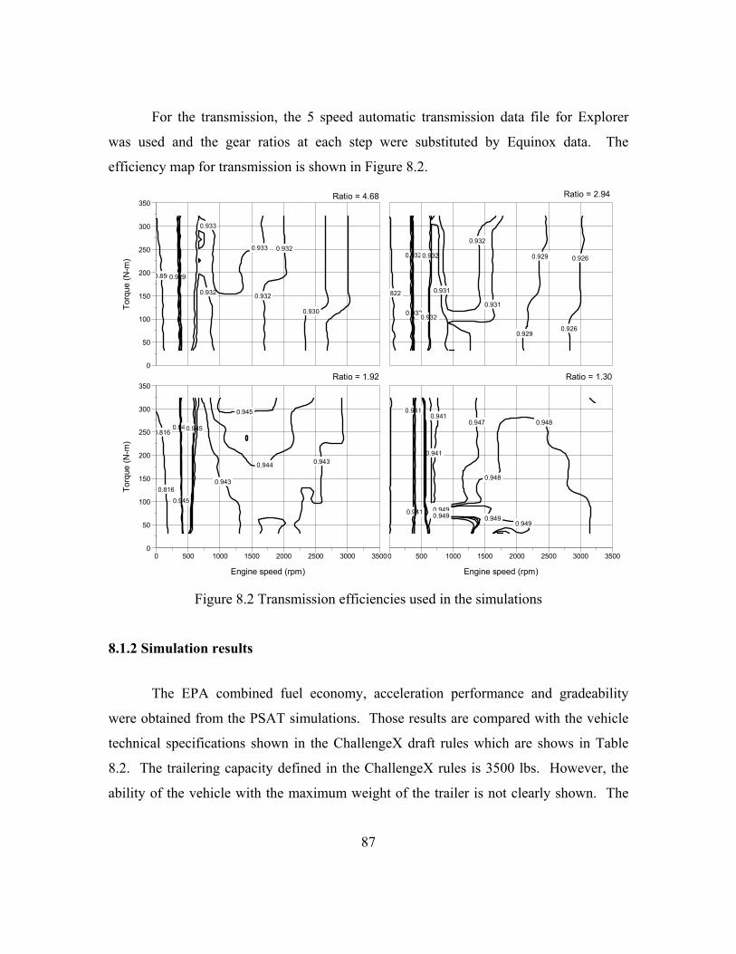
For the transmission, the 5 speed automatic transmission data file for Explorer
was used and the gear ratios at each step were substituted by Equinox data. The
efficiency map for transmission is shown in Figure 8.2.
Torq
ue (N
-m)
0
50
100
150
200
250
300
350
0.8560.929
0.930
0.932 0.932
0.932
0.933
0.933
Ratio = 4.68
.822
0.932
0.9320.932
0.932
0.932
0.929
0.929 0.926
0.926
0.931
0.931
Ratio = 2.94
Torq
ue (N
-m)
0
50
100
150
200
250
300
350
Engine speed (rpm)
0 500 1000 1500 2000 2500 3000 3500
0.816
0.816
0.945
0.945
0.945
0.945
0.944
0.943
0.943
Ratio = 1.92
Engine speed (rpm)
0 500 1000 1500 2000 2500 3000 3500
0.941
0.9410.941
0.941
0.941
0.9470.947
0.947
0.9480.948
0.948
0.948
0.9490.949 0.949
0.949
Ratio = 1.30
Figure 8.2 Transmission efficiencies used in the simulations
8.1.2 Simulation results
The EPA combined fuel economy, acceleration performance and gradeability
were obtained from the PSAT simulations. Those results are compared with the vehicle
technical specifications shown in the ChallengeX draft rules which are shows in Table
8.2. The trailering capacity defined in the ChallengeX rules is 3500 lbs. However, the
ability of the vehicle with the maximum weight of the trailer is not clearly shown. The
87

author followed the PNGV performance guidelines and assumed that the gradeability of
the vehicle with trailer (3500 lbs) must be the ability to climb a grade higher than 6.5%.
Table 8.2 Selected vehicle technical specifications in ChallengeX and PNGV performance guidelines
Vehicle technical specifications in ChallengeX rules Description Base vehicle (V6) Competition requirement
0-60 mph 8.9 sec 9.0 sec 50-70 mph 6.8 sec 6.8 sec Vehicle mass 4000 lbs 4400 lbs MPG combined EPA
23.3 mpgge 32.0 mpgge
Highway range 320 miles 200 miles Passenger capacity 5 passenger 5 passenger Emission cert. level Tier 2, Bin 5 - Trailering capacity 3500 lbs 2500 lbs Starting time < 2.0 sec < 5.0 sec
PNGV guidelines Description Requirement
0-60 mph 12 sec 0-85 mph 25 sec 40-60 mph 5.3 sec Maximum speed 85 mph Gradeability, forward & reverse 30% at GVW Gradeability, forward 6.5% @55mph for 20
minutes (GVW with full accessory load)
The screenshots for a PSAT simulation are shown in Figure 8.3. The first screen
is for the construction of the test vehicle. The configuration and data file for each
component is set in this screen. The second one is for the test cycle. It determines the
driving cycle or performance test on which the constructed vehicle is to be tested. It is
possible to simulate for multiple driving cycles and multiple performance testing. The
application of the SOC (State of Charge) correction algorithm is also determined here.
The screenshot shown in Figure 8.4 is the result screen. The fuel economy and emissions
data are shown. The acceleration performance can be known from this screen, too.
88

(a) Input data screen
(b) Simulation condition screen
Figure 8.3 Screenshots for the simulation of conventional the Equinox
89
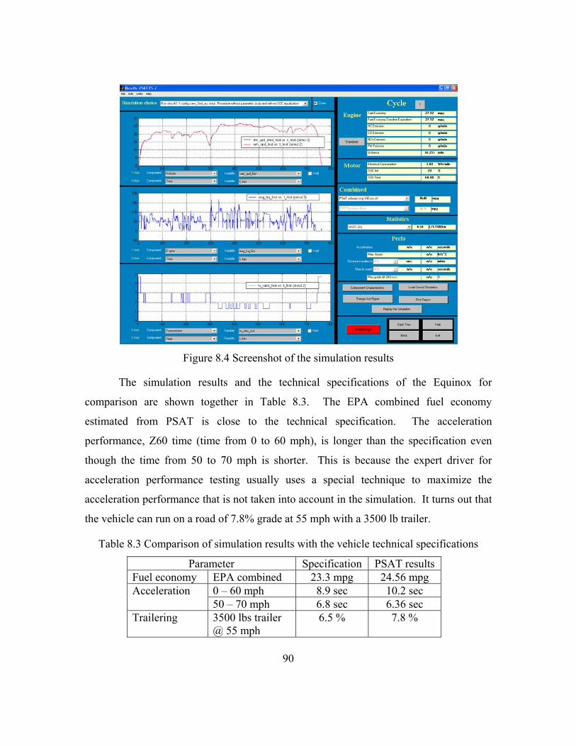
Figure 8.4 Screenshot of the simulation results
The simulation results and the technical specifications of the Equinox for
comparison are shown together in Table 8.3. The EPA combined fuel economy
estimated from PSAT is close to the technical specification. The acceleration
performance, Z60 time (time from 0 to 60 mph), is longer than the specification even
though the time from 50 to 70 mph is shorter. This is because the expert driver for
acceleration performance testing usually uses a special technique to maximize the
acceleration performance that is not taken into account in the simulation. It turns out that
the vehicle can run on a road of 7.8% grade at 55 mph with a 3500 lb trailer.
Table 8.3 Comparison of simulation results with the vehicle technical specifications
Parameter Specification PSAT results Fuel economy EPA combined 23.3 mpg 24.56 mpg
0 – 60 mph 8.9 sec 10.2 sec Acceleration 50 – 70 mph 6.8 sec 6.36 sec
Trailering 3500 lbs trailer @ 55 mph
6.5 % 7.8 %
90

Except for minor discrepancies, the PSAT results seem to be reliable for the
estimation of fuel economy and performances. These data will be used as the baseline
data to determine the size of the components of the virtual HEV.
8.2 HEV MODELING
8.2.1 Component sizing
The conventional Equinox is a high performance vehicle satisfying a number of
standards for acceleration performance, gradeability (hill-climbing ability), sustained
high speed and driving range. It is necessary to find out the combination
engine/battery/motor satisfying the performance guidelines. The starting point is the
engine sizing to at least satisfy the gradeability requirement since the long duration of this
requirement implies that the engine has the capability of gradeability by itself. The
battery and motor are then to be sized to allow the vehicle to meet acceleration
performance. The gradeability is not yet clearly defined in the ChallengeX rules.
Instead, the trailering capacity is defined. Therefore, the author designed the virtual HEV
which has the performance specifications shown in Table 8.4. The required Z60 time is
9.0 seconds in the given specifications. However, the simulated Z60 time can be reduced
in the actual vehicle testing. The allowable Z60 time in simulation is assumed to be the
same as that of the stock vehicle, 10.2 seconds.
Table 8.4 Criteria for component sizing
Component Required performance Specification Engine Gradeability @ 55 mph
with GVW + trailer More than 6.5% gradeability
with 2500 lbs trailer Motor/Battery 0-60 mph 9.0 (10.2) seconds
Various combinations of engine/battery/motor were simulated to find out the
combination which can satisfy the performance requirement. At first, the engine of the
OPA was tested to determine if it can satisfy the trailering capacity without changing the
maximum power of the engine. Then the combination of motor and battery was selected
91

to meet the required acceleration performance. The combination found as results of the
simulations are shown in Table 8.5 with the simulation results.
It turns out that the 112kW DISI engine in the OPA can satisfy the trailering
capacity requirement by itself. The 30kW UQM motor with Ovonic battery were
selected as their combination has the least power and capacity as well as the ability to
satisfy the performance requirement.
Table 8.5 Combination of engine/motor/battery to satisfy performance guidelines
Specification Comp-onent
Manufacturer Type Maximum power/Capacity
File name in PSAT
Engine Toyota DISI 112 kW Eng_si_2000_112_opa Motor Unique
Mobility PM Induction motor/inverter
30 kW mc_pm_30
Battery Ovonic NiMH 28 A-hr Ess_nimh_28_300_ovonic
Performance PSAT results
Parameter Specification Stock vehicle
Virtual HEV
0-60 mph 9.0 sec 10.2 sec 10.21 sec Acceleration 50-70 mph 6.8 sec 6.4 sec 5.7 sec
Trailering capacity
Gradeability @ 55 mph with 3500 lbs (stock vehicle) with 2500 lbs (virtual HEV)
6.5 % 7.8 % 6.5 %
92

8.2.2 HEV model for simulation
The base vehicle for simulation is the Equinox and the parallel 2-wheel drive
configuration was selected as the HEV system to be simulated. The configurations and
the specifications of the components used are shown in Table 8.6.
Table 8.6 Configurations and components used
Configuration
Battery
Engine Motor
Clutch Transmission Final drive WheelsBattery
Engine Motor
Clutch Transmission Final drive Wheels
Components specifications Component Parameter Specification
Frontal area 3.19 m2 Drag coefficient 0.417
Vehicle
Rolling resistance coefficient 0.0084 Displacement 1998 cc Type Direct Injection Spark Ignition Maximum power 112 kW @ 6000 rpm Maximum torque 200 N-m @ 4000 rpm Efficiency map Figure 6.7
Engine
Emissions maps Figure B.2 ~ B.3 Type 3 way + DeNOx catalyst Catalyst Efficiency Figure 8.6 Type 5 speed manual transaxle Transmission Gear ratios 3.2 - 2.3 - 1.5 - 1.0 - 0.75
Final drive Reduction ratio 3.24 Continuous maximum power 30 kW Continuous maximum torque 305 N-m
Motor
Efficiency map Figure 8.5 Battery Capacity 28 A-hr
93

The efficiency map and the maximum torque curve of the motor used are shown
in Figure 8.5. The efficiency of the catalyst is defined as a function of temperature. The
catalyst efficiency was approximated based on the obtained conversion efficiency during
the FTP cycle and shown in Figure 8.6.
To
rque
(N-m
)
0
100
200
300
400
Rotational speed (rpm)
0 1000 2000 3000 4000 5000 6000
0.86
0.86
0.86
0.86
0.86
0.86
0 85
0.85
0.85
0.85
0.85
0.85
0.85
0 850 85
0.74 0.74 0.74
0.740.740.740.74
0.82 0.82 0.82
0.82
0.82
0.82
0 82
0.82
0 82
0.70 0.70 0.70
0.90
0.90
0.90
0.90
0.90
0.90
Peak maximum torque
Continuous maximum torque
Figure 8.5 Characteristics of used motor
Catalyst temperature ( C)
0 100 200 300 400 500 600 700 800 900
HC
Stoichiometric Lean
Mapped efficiency (Lean) Mapped efficiency (Stoichiometric)
Con
vers
ion
effic
ienc
y (%
)
0
20
40
60
80
100
Catalyst temperature ( C)
0 100 200 300 400 500 600 700 800 900
NOx
Stoichiometric Lean
Mapped efficiency
(a) HC (b) NOx
Figure 8.6 Catalyst efficiency curve
94

8.2.3 Simulation results
The hybridization results in an increase in vehicle weight. The gross vehicle
weight of the Equinox is 4000 lbs and that of the hybridized Equinox is calculated based
on the added components and found to be around 4400 lbs, which is the regulated weight
defined in the ChallengeX rule. Therefore, the test weight of hybrid Equinox was set as
4400 lbs.
The fuel economy results from the PSAT simulations are summarized in Table
8.7. Even with the increased vehicle weight, the fuel economy is improved by more than
10 % due to the hybridization. The fuel economy improvement by adoption of a DISI
engine instead of a conventional SI engine is found to be 4.2 % in terms of composite
fuel economy.
Table 8.7 Fuel economy simulation results
Conventional HEV with SI engine
HEV with DISI engine
Vehicle weight 4000 lbs 4400 lbs 4400 lbs FTP 22.37 25.44 26.93 HWFET 27.92 30.39 30.99 Fuel economy
(mpg) Composite 24.56 27.45 28.61 Improvement over conventional powertrain - 11.8 % 16.5 % Improvement over HEV with SI engine - - 4.2 %
To see in detail the contributing factors on the fuel economy improvement due to
the hybridization, the energy loss at each component was calculated. In this calculation,
only Phase 3 was considered. The fuel consumption of the conventional vehicle was
446.8 g and that of the HEV was 381.0 g. The difference of consumed fuel is 65.8 g and
the corresponding energy difference is 2906 kJ. The calculated energy losses are shown
in Figure 8.7. It is seen that there are three positive factors and one negative factor. The
energy loss in the engine decreases as the engine size decreases. The reduced engine size
makes the operating points closer to the most efficient region and increases the overall
efficiency. The transmission loss decreases as the transmission changes from the
automatic to the manual transmission. The energy loss for the vehicle increases because 95

the weight increases. Turning off the engine when power is not required (idle engine
stop) is effective to decrease the fuel consumption during idle and braking.
0
3000
6000
9000
12000
15000
Engine TM Vehicle Idle & braking
Components
Ener
gy (k
J)
Conventional Parallel HEV
Engine efficiency increase by down sizing
Automatic to manual transmission
Vehicle weight increase
Idle enginestop
Figure 8.7 Energy losses for each component
The savings of fuel consumption for each factor are quantified and shown in
Table 8.8. The savings in the engine including the savings for idle and braking is found
to be the dominant factor on the fuel economy improvement due to the hybridization.
The sum of these two factors is about 88% of the total savings.
Table 8.8 Contribution of each factor on the fuel economy improvement
due to the hybridization
Components Engine Transmi-ssion
Vehicle Idle & braking
Regenerated energy
Contributions 60.2% 11.7% -12.9% 28.4% 12.6%
96

In Table 8.7, the fuel economy improvement from the DISI engine was found to
be 4.2% in terms of composite fuel economy and that improvement during Phase 3 of the
FTP was found to be 3.9%. This improvement is less than that of conventional vehicle
mentioned in the previous chapter. In the previous chapter, the benefit of fuel economy
of the OPA engine in the lean combustion mode over the stoichiometric mode was found
to be 5.7% for both the experiment and simulation.
The overall engine efficiencies were calculated from the history of input and
output power flows during the power mode and the following efficiencies were obtained.
• SI engine : 29.8%
• DISI engine : 30.3%
The difference in the overall efficiency of a DISI engine in a conventional vehicle
(mentioned in the previous chapter: 1.2 percentage points) and that in an HEV is 0.5
percentage points. This is because the HEV engine operating points are primarily located
in the high load region. In the HEV, the engine is down sized so the engine has to work
in the high torque region at the same power requirement from the vehicle. Figure 8.8
shows the engine operating points on the BSFC map during the 505 cycle for both the
DISI engine and SI engine in an HEV.
BM
EP (b
ar)
0
2
4
6
8
10
12
Engine speed (rpm)
500 1000 1500 2000 2500 3000
265
265265
265
294294
294294
270
270
270
270280
280
280
280280280
320320320
Leanoperation region
Maximum performance
Engine speed (rpm)
500 1000 1500 2000 2500 3000
265
265 265
300300300
270
270
270
270
320320320
370370370
340 340 340
Maximum performance
(a) DISI engine (b) SI engine
Figure 8.8 Engine operating points of an HEV
97

It is shown that the DISI engine operating points within the lean operation region
are less than those in the case of the conventional vehicle shown in Figure 7.17. The
dwell times in the lean combustion mode of the DISI engine for both the conventional
and HEV are shown in Table 8.9. It is shown that the time in the lean combustion mode
of the DISI engine for the HEV is less than one third of that for a conventional vehicle.
As a result of that, the fuel economy improvement from use of a DISI engine in an HEV
is not as high as might be anticipated because the down-sized DISI engine operates
primarily in homogeneous charge mode.
Table 8.9 Dwell time in lean combustion mode of DISI engine during 505 cycle
Engine power mode
In lean combustion mode
Ratio of lean combustion mode
Conventional 297 sec 189 sec 64 % HEV 284 sec 56 sec 20 %
The emissions of two HEVs with different types of engines were calculated
during the Hot 505 cycle and shown in Table 8.10. The HCs from the two HEVs are
similar to each other. However, the NOx from the DISI engine is higher than that of the
SI engine. This is mostly due to the worse efficiency of the lean NOx catalyst.
Table 8.10 Simulated emissions of HEVs with SI and DISI engines (g/mile)
HC NOx SI engine 0.027 0.193
DISI engine 0.026 0.243
During the Hot 505 cycle, the use of a DISI engine in a parallel-type HEV
application results in an improvement of fuel economy by 3.9% but 26% higher the NOx
emissions and similar HC emissions.
8.3 CHAPTER SUMMARY
The fuel economy benefit of a DISI engine in an HEV application was evaluated
for a virtual HEV which will be used in the ChallengeX competition. PSAT was used as
98

a simulation tool to calculate the fuel economy, emissions and performance for the given
powertrain configuration and components.
The validity of the simulation was checked by comparing the simulated results
with the vehicle specifications and test data. It is concluded that PSAT can predict the
performance within an allowable error range. The sizes of the components were
determined based on the performance requirements defined in the ChallengeX rules. The
required maximum engine power was determined based on the gradeability with the
specified maximum trailer. The 112kW engine in the OPA was found to be enough to
satisfy that requirement without scaling of maximum power. Then the sizes of the
motor/battery were determined so that the combination of engine/motor/battery can
accomplish the specified acceleration performance of Z60 time. As results from the
PSAT simulations, it was found that the combination of a 30kW PM induction motor and
a 28A-h NiMH battery can satisfy the acceleration requirement.
The fuel economy improvement by hybridization was found to be a 12% increase
in EPA composite fuel economy. The factors on the fuel economy improvement were
analyzed and it was found that the fuel savings in the engine is a dominant factor
responsible for 88% of the improvement.
The benefit of a DISI engine over a conventional SI engine in an HEV application
is found to be 4.2% in terms of composite fuel economy and 3.9% for the Hot 505 cycle,
which is less than that of 5.7% for a DISI engine in a conventional vehicle. The overall
engine efficiency improvement of a DISI engine in an HEV application is 0.5 percentage
points which is also less than that for a DISI engine in a conventional vehicle application.
This is because the engine is working in the high load region due to the down-sized
engine. This DISI engine operates primarily in homogeneous charge mode for high load,
and thus does not offer a large fuel economy benefit. The HC emissions of both types of
engines are similar to each other and the NOx emissions of HEV with a DISI engine is
26% higher than that with an SI engine.
99

CHAPTER 9: SUMMARY AND CONCLUSIONS
A Toyota OPA was selected as a test vehicle as it has the components of interest:
a Direct Injection Spark Ignition (DISI) engine and a Continuously Variable
Transmission (CVT). In order to estimate the benefit of the DISI engine and CVT, a
2001MY Toyota OPA was tested to collect the engine and CVT maps using in-situ
measurement techniques. Three torque sensors were installed into the powertrain in the
vehicle for that purpose; one is between the engine and transmission and the other two
are installed on the drive axles. The overall efficiency of the engine and transmission
was estimated using the measured torques and speeds during Phase 3 of the FTP cycle.
The overall efficiencies of the engine at different operating modes including the lean and
stoichiometric combustion modes were compared to each other. The overall efficiencies
of the CVT are analyzed similarly. Finally, the measured steady state efficiency maps
and emissions maps were used to predict the fuel economy and emissions of an HEV
with the DISI engine and CVT.
9.1 CONCLUSIONS
1. Fuel economy and emissions of the OPA
2nd generation D4 – 30.5 mpg
FTP emissions
o HC – 0.141 g/mile
o NOx – 0.245 g/mile
o CO – 1.114 g/mile
2. Toyota has made considerable improvements in tailpipe HC and NOx
emissions with their second generation D-4 engine. For the HC emissions, the
change in combustion system using their slit nozzle injector is the dominant
factor. The dominant factor for the NOx emissions turns out to be the
significantly improved catalyst efficiency.
100

3. Even with the improvement for the emissions reductions, the barriers to the
U.S. market still remain high for the DISI engine. The tailpipe NMOG and
NOx do not meet the LEV standards in the NLEV program.
4. Using the in-situ mapping technique, the map data for the engine and
transmission was successfully obtained. This in-situ mapping is a promising
tool.
5. The engine-out HC emissions in terms of BSHC for lean combustion are 2~3
times of that in the stoichiometric combustion mode. The engine-out NOx
emissions are about one-half to one-sixth compared to that in the
stoichiometric combustion mode.
6. Both the PSAT and ADVISOR predictions for the power flows, speeds and
torques of each component agree well with the measured results.
7. It is concluded that the fuel economy benefit of a DISI engine over a PFI
engine is 5.7% due to the 3.4 percentage points improvement in the overall
engine efficiency.
8. The fuel economy benefit of a DISI engine over a PFI engine in an HEV
application during Phase 3 of the FTP cycle is found to be 3.9%.
9. The fuel economy benefit of a DISI engine in an HEV application is found to
be less than that for a DISI engine in a conventional vehicle application. This
is because the engine is working in the high load region where the engine is in
the stoichiometric combustion mode due to the downsized engine.
10. The tailpipe HC emission from a DISI engine in an HEV are about the same as
those from a conventional SI engine in an HEV, but the tailpipe NOx emission
are 26% higher.
9.2 RECOMMENDATIONS FOR FUTURE WORK
This dissertation research focused on the evaluation of the fuel economy benefit
of the newly introduced DISI engine and CVT transmission using in-situ power flow
101

measurements. The power flow measurement technique is also applicable to compare the
efficiency of the engine or transmission of two competing vehicles. The feasibility of the
DISI engine in an HEV was tested using a simulation tool in a virtual vehicle. The
simulation results are compared with the experimental results and the simulation
approach is found to be reliable for the estimation of the fuel economy benefit.
Therefore, the further direction can be either refinement or applications of this approach.
Even though the application of the DISI engine in an HEV is found to be less effective
than that in a conventional vehicle, there should be a way to maximize the benefit of the
DISI engine in an HEV. Several topics for further research are addressed below.
9.2.1 Finding a way to maximize the benefit of a DISI engine in an HEV application
There are various configurations and control strategies in HEVs. In the present
research, only the parallel 2 wheel drive HEV with the default control strategy in PSAT
was simulated to examine the effect of the DISI engine. The other configuration, with a
control strategy which takes into account the efficiency characteristics of the DISI
engine, will be able to improve the fuel economy of an HEV with the DISI engine.
9.2.2 Refinement of engine torque measuring technique
The engine torque measurement in a vehicle is one of the most important
techniques used in this dissertation research. This in-situ torque measurement technique
has various applications in vehicle development. The problem of this method is time and
cost of torque sensor installation. In the application to the OPA, it took four months to
install the torque sensor between the engine and CVT. The finite length of the torque
sensor increases the total length of the powertrain so the mounting has to be changed.
Therefore, the best way to reduce the mechanical work is to use a zero clearance torque
sensor which can eliminate the engine room work.
102

9.2.3 Correlation of engine efficiency with the vehicle’s fuel economy
One of the questions of the engine designer is how the change in the BSFC map
affects the actual vehicle fuel economy. The BSFC map is obtained from steady state
engine dynamometer testing and the fuel economy comes from transient chassis
dynamometer testing. As the fuel economy is the combined result of all powertrain
components, it is not clear yet how the engine dynamometer test result is related to the
vehicle test results. If the simulation tool is refined and validated by comparing the
simulation results with the measured results, it would be possible to predict precisely the
change in fuel economy given only the two BSFC maps.
103

APPENDIX A FTP TEST RESULTS
The following graphs are the measured engine data and emissions data during the
FTP test. Except for the issues discussed in the main chapters, the other variables are
presented here
Veh
icle
spe
ed (m
ph)
0
20
40
60
Fuel
flow
rate
(g/s
ec)
0
1
2
3
Time (sec)
0 100 200 300 400 500
AF
ratio
0
10
20
30
40
Acce
l. po
sitio
n T
hrot
tle p
ositi
on (V
)
0
1
2
3
4
(a) Phase 1
Figure A.1 Engine operation during the FTP cycle 104

Veh
icle
spe
ed (m
ph)
0
20
40
60
Fuel
flow
rate
(g/s
ec)
0
1
2
3
Time (sec)
500 700 900 1100 1300
AF
ratio
0
10
20
30
40
Acc
el. p
ositi
on
Thro
ttle
posi
tion
(V)
0
1
2
3
4
(b) Phase 2
Figure A.1 Engine operation during the FTP cycle
105

Veh
icle
spe
ed (m
ph)
0
20
40
60
Fuel
flow
rate
(g/s
ec)
0
1
2
3
Time (sec)
0 200 400
AF
ratio
0
10
20
30
40
Acc
el. p
ositi
on
Thro
ttle
posi
tion
(V)
0
1
2
3
4
(c) Phase 3
Figure A.1 Engine operation during the FTP cycle
106

Veh
icle
spe
ed(m
ph)
0
20
40
60E
xhau
st te
mpe
ratu
re (
C)
0
200
400
600
800
Time (sec)
0 200 400 600 800 1000 1200
Before catalyst After catalyst
Time (sec)
0 100 200 300 400 500
Figure A.2 Exhaust gas temperature during the FTP cycle
Veh
icle
spe
ed(m
ph)
0
20
40
60
Cat
alys
t tem
pera
ture
( C
)
0
200
400
600
800
1000
Time (sec)
0 200 400 600 800 1000 1200
Front catalyst Rear catalyst
Time (sec)
0 100 200 300 400 500
Figure A.3 Catalyst temperature during the FTP cycle
107

Veh
icle
spe
ed(m
ph)
0
20
40
60Ai
r fue
l rat
io
0
10
20
30
40
HC
(g/s
ec)
0.00
0.02
0.04
0.06
0.08
HC
(g/s
ec)
0.00
0.01
0.02
0.03
Time (sec)
500 700 900 1100 1300
HC
(g/s
ec)
0.00
0.02
0.04
0.06
0.08
Air f
uel r
atio
0
10
20
30
40
HC
(g/s
ec)
0.00
0.01
0.02
0.03
Time (sec)0 100 200 300 400 500
Figure A.4 Engine-out and Tailpipe THCs during the FTP cycle
108
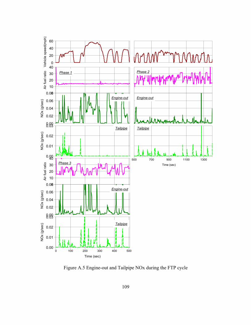
Veh
icle
spe
ed(m
ph)
0
20
40
60A
ir fu
el ra
tio
0
10
20
30
40Phase 1
NO
x (g
/sec
)
0.00
0.02
0.04
0.06
0.08Engine-out
Phase 2
Engine-out
NO
x (g
/sec
)
0.00
0.01
0.02
0.03 Tailpipe
Time (sec)
500 700 900 1100 1300
Tailpipe
NO
x (g
/sec
)
0.00
0.02
0.04
0.06
0.08Engine-out
Air
fuel
ratio
0
10
20
30
40Phase 3
NO
x (g
/sec
)
0.00
0.01
0.02
0.03
Time (sec)0 100 200 300 400 500
Tailpipe
Figure A.5 Engine-out and Tailpipe NOx during the FTP cycle
109

Veh
icle
spe
ed(m
ph)
0
20
40
60A
ir fu
el ra
tio
0
10
20
30
40Phase 1
CO
(g/s
ec)
0.0
0.1
0.2
0.3Engine-out
Phase 2
Engine-out
CO
(g/s
ec)
0.00
0.05
0.10
0.15Tailpipe
Time (sec)
500 700 900 1100 1300
Tailpipe
CO
(g/s
ec)
0.0
0.1
0.2
0.3Engine-out
Air
fuel
ratio
0
10
20
30
40Phase 3
CO
(g/s
ec)
0.00
0.05
0.10
0.15
Time (sec)0 100 200 300 400 500
Tailpipe
Figure A.6 Engine-out and Tailpipe CO during the FTP cycle
110

Veh
icle
spe
ed (m
ph)
0
20
40
60
HC
Effi
cien
cy(%
)
0
25
50
75
100
NO
x Ef
ficie
ncy(
%)
0
25
50
75
100
CO
Effi
cien
cy (%
)
0
25
50
75
100
Time (sec)0 100 200 300 400 500
Cat
alys
t tem
pera
ture
( C
)
0
200
400
600
800
1000
Front catalyst Rear catalyst
(a) Phase 1 Figure A.7 Catalyst efficiencies during the FTP cycle
111
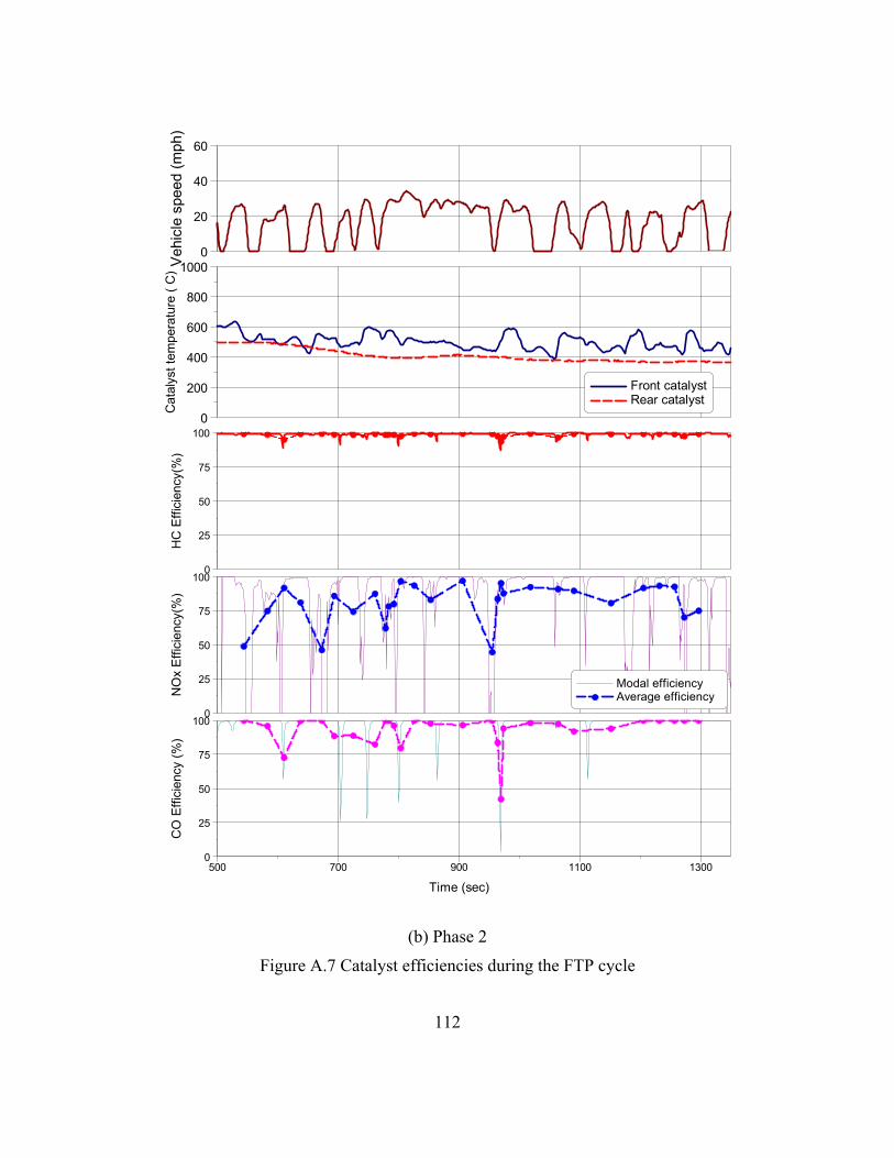
Veh
icle
spe
ed (m
ph)
0
20
40
60
HC
Effi
cien
cy(%
)
0
25
50
75
100
NO
x E
ffici
ency
(%)
0
25
50
75
100
Modal efficiency Average efficiency
CO
Effi
cien
cy (%
)
0
25
50
75
100
Time (sec)500 700 900 1100 1300
Cat
alys
t tem
pera
ture
( C
)
0
200
400
600
800
1000
Front catalyst Rear catalyst
(b) Phase 2
Figure A.7 Catalyst efficiencies during the FTP cycle
112

Veh
icle
spe
ed (m
ph)
0
20
40
60H
C E
ffici
ency
(%)
0
25
50
75
NO
x E
ffici
ency
(%)
0
25
50
75
CO
Effi
cien
cy (%
)
0
25
50
75
Time (sec)0 100 200 300 400 500
Cat
alys
t tem
pera
ture
( C
)
0
200
400
600
800
1000
Front catalyst Rear catalyst
(c) Phase 3
Figure A.7 Catalyst efficiencies during the FTP cycle
113

APPENDIX B STEADY STATE TEST RESULTS
The following graphs are the measured engine and emissions data maps obtained
during the steady state test. Except for the issues discussed in the main chapters, the
other variables are presented here
Lean combustion
BM
EP (b
ar)
0
2
4
6
8
10
12
Engine speed (rpm)
500 1000 1500 2000 2500 3000
265
265265
265
294294
294294
270
270
270
270280
280
280
280280280
320320320
Leanoperation region
Maximum performance
Stoichiometric combustion
BME
P (b
ar)
0
2
4
6
8
10
12
Engine speed (rpm)
500 1000 1500 2000 2500 3000
265
265 265
300300300
330330330
270
270
270
270
320320320
370370370
Maximum performance
Figure B.1 Brake specific fuel consumption maps
114

Stoichiometric mode
Lean mode
BM
EP
(bar
)
1
2
3
4
5
6
Engine speed (rpm)
1000 1500 2000 2500 3000
2.92
2.92
2.922.67
2.67 3.07
3.07
3.073.07
BM
EP
(bar
)
1
2
3
4
5
6
Engine speed (rpm)
1000 1500 2000 2500 3000
3.63.63.6
5.15.1
5.1
5.1
5.1
7.47.4
7.4
7.4
Figure B.2 Brake specific HC maps
115

Stoichiometric mode
Lean mode
BM
EP
(bar
)
1
2
3
4
5
6
Engine speed (rpm)
1000 1500 2000 2500 3000
2.0
2.0
2.03.1
3.1
3.1 4.64.6
4.64.6
4.6
4.6
4.64.6
BME
P (b
ar)
1
2
3
4
5
6
Engine speed (rpm)
1000 1500 2000 2500 3000
16.916.9
16.9
16.9
16.9
16.9
13.4
14.2
14.2
14.2
Figure B.3 Brake specific NOx maps
116

Stoichiometric mode
Lean mode
BM
EP
(bar
)
1
2
3
4
5
6
Engine speed (rpm)
1000 1500 2000 2500 3000
33
33
33
3333
33
33
43
43 43
27
27
BMEP
(bar
)
1
2
3
4
5
6
Engine speed (rpm)
1000 1500 2000 2500 3000
25.3
25.3
25.3
25.3
28.528.5
28.5
28.5
28.5
28.5
31.4
31.4
Figure B.4 Specific CO map
117

Stoichiometric mode Lean mode
MAP (kPa)
Volumetric efficiency (-)
Engine speed (rpm)
1000 1500 2000 2500 3000
95
95
95
7070
70
5858
58
81
81
8190
90
90
BM
EP
(bar
)
1
2
3
4
5
6
Engine speed (rpm)
1000 1500 2000 2500 3000
35 35 35
42 42 42
52 52 52
60 60 60
70 70 70
BM
EP
(bar
)
1
2
3
4
5
6
Engine speed (rpm)
1000 1500 2000 2500 3000
0.500.500.50
0.430.430.43
0.360.360.36
0.290.290.29
0.240.240.24
Stoichiometric mode
Engine speed (rpm)
1000 1500 2000 2500 3000
0.620.62
0.62
0.56
0.560.560.520.52
0.52
0.410.410.41
Lean mode
Figure B.5 MAP and volumetric efficiency
118

Lean modeStoichiometric mode
Ignition timing (deg BTDC)
Injection timing (deg. BTDC)Engine speed (rpm)
1000 1500 2000 2500 3000
22.6
19.6
19.6
19.6
19.6
19.0
19.0
19.0
19.0
16.1
16.1
16.1
BM
EP
(bar
)
1
2
3
4
5
6
Engine speed (rpm)
1000 1500 2000 2500 3000
25.8
25.8
25.8
28.1 28.1
19.1
19.1
19.1
21.4
21.4
21.4
BME
P (b
ar)
1
2
3
4
5
6
Engine speed (rpm)
1000 1500 2000 2500 3000
310
310
310
320 320
300
300
Stoichiometric mode
Engine speed (rpm)
1000 1500 2000 2500 3000
51.9
59.6
59.6
63.0
63.0
67.4
67.4
Lean mode
Figure B.6 Ignition timing and injection timing
119
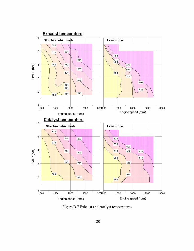
Exhaust temperature
Catalyst temperature
BME
P (b
ar)
1
2
3
4
5
6
Engine speed (rpm)
1000 1500 2000 2500 3000
450
480
480480
480
520
520
520
550
550
550
590
590
620
Engine speed (rpm)1000 1500 2000 2500 3000
460
460
460
430
430
430
420
420
360
BM
EP (b
ar)
1
2
3
4
5
6
Engine speed (rpm)
1000 1500 2000 2500 3000
800
760
760
720
720
720
670
670
670
600
Stoichiometric mode
Engine speed (rpm)
1000 1500 2000 2500 3000
460
460
510
510
510
570
570
570
620
620
620
Stoichiometric mode
Lean mode
Lean mode
Figure B.7 Exhaust and catalyst temperatures
120

REFERENCE
1. Alkidas, A. and S. El Tahry (2003), “Contributors to the Fuel Economy Advantage of DISIE Engines Over PFI Engins”, SAE Paper 2003-01-3101
2. Amann, C. (1997), “The Stretch for Better Passenger-Car Fuel Economy”, SAE Paper 972658
3. An, F., F. Stodolsky, and D. Santini (1999), “Hybrid Options for Light-Duty Vehicles”, SAE Paper 1999-01-2929.
4. Anderson, R., D. Brehob, J. Yang, J. Vallance, R. Whitaker, “A New Direct Injection Spark Ignition Combustion System for Low Emission” FISITA-96, No. P0201
5. Anon. (1994), “PNGV Program Plan”, U.S. Dept. of Commerce, Washington, DC, and USCAR, Dearborn, MI (July 1994)
6. Brehob, D.D., J. Fleming, M. Haghgooie, R.A. Stein (1998), “Stratified charge Engine Fuel Economy and Emission Characteristics”, SAE Paper 982704
7. Carney, D. (2004), “Internal Combustion Engineering”, SAE Automotive Engineering International, 1997, No. 5, pp 39-46
8. Cole, R. C., R.B.Poola, and R. Sekar (1998), “Exhaust Emissions of a Vehicle with a Gasoline Direct-Injection Engine”, SAE Paper 982605
9. Corsetti, A., G. O’Connell, K. Watkins (2002), “In-vehicle Torque Model Validation”, SAE Paper 2002-01-1143
10. Davis, S.C. and S.G. Strang (1993), “Transportation energy data book: Edition 13”, Report ORNL-6743, Oak Ridge National Laboratory,
11. Decicco, J. and M. Ross (1996),”Recent advances in automotive technology and cost-effectiveness of fuel economy improvement”, Transportation Research Part D (2), 79-96
12. Duoba, M., H. Ng and R. Larsen (2000), “In-situ mapping and analysis of the Toyota Prius HEV engine”, SAE Paper 2000-01-3096
13. Duoba, M., H. Ng and R. Larsen (2001) “Characterization and comparison of two hybrid electric vehicles (HEVs) – Honda Insight and Toyota Prius”, SAE Paper 2001-01-1335
121

14. Fraidl, G., W. Piock, M. Wirth (1996), “Gasoline Direct Injection: Actual Trends and Future Strategies for Injection and Combustion System”, SAE Paper 960465
15. Hachisuka, I., H. Hirata, Y. Ikeda, S. Matsumoto, “Deactivation Mechanism of NOx Storage-Reduction Catalyst and Improvement of Its Performance”, SAE Paper 2000-01-1196
16. Harada, J., T. Tomita, H. Mizuno, Z. Mashiki, Y. Ito (1997), “Development of Direct Injection Gasoline Engine”, SAE Paper 970540
17. Ikeda, Y. (1999), “Development of NOx storage Reduction Catalyst for Direct Injection Gasoline Engine”, SAE Paper 991279
18. Kanda, M., T. Baika, S. Kato, M. Iwamuro, M. Koike, A. Saito(2000), “Application of a New combustion Concept to Direct Injection Gasoline Engine”, SAE Paper 2000-01-0531
19. Karnopp, D., D. Margolis, R. Rosenberg (2000), System Dynamics 3rd ed., John Wiley & Sons, New York, ,
20. Karl, G., R. Kemmler, M. Bargende (1997), “Analysis of a Direct Injected Gasoline Engine”, SAE Paper 970624
21. Kluger, M. A. and D. M. Long (1999), “An Overview of Current Automatic, Manual and Continuous Variable Transmission Efficiencies and their Projected Future Improvement”, SAE Paper 1999-01-1259
22. Kluger, M. A. and Fussner, D. R. (1997). An overview of current CVT mechanisms, forces and efficiencies. SAE Technical Paper 970688.
23. Koike, M., A. Saito, T. Tomoda, Y. Yamamoto, “Research and Development of a New Direct Injection Gasoline Engine”, SAE Paper 2000-01-0530
24. Krebs, R., E. Pott, T.P. Kreuzer, U. Gobel, K. Gluck (2002),”Exhaust Gas Aftertreatment of Volkswagen FSI Fuel Stratified Injection Engines”, SAE Paper 2002-01-0346
25. Kume, T., Y. Iwamoto, K. Iida, M. Murakami, K. Akishino, H. Ando (1996), “Combustion Control Technologies for Direct Injection SI engine”, SAE Paper 960600
26. Kuwahara, K., T. Watanabe, T. Shudo, H. Ando (1996), “A Study of Combustion Characteristics in a Direct Injection Gasoline Engine by High Speed Spectroscopic Measurement”, Proceedings of the Internal Combustion Engine Symposium – Japan (in Japanese),1996, pp145-150
122

27. Lindhjem, C.E. (1997), “Conversion Factors for Hydrocarbon Emission Components,” U.S. EPA Office of Mobile Sources Report No. NR-002
28. Markel, T., A. Brooker, T. Hendricks, V. Johnson, K. Kelly, B. Kramer, M. O’Keefe, S. Sprik, K. Wipke (2002), “ADVISOR: A system analysis tool for advanced vehicle modeling”, Journal of Power Sources, Vol. 4801 pp 1-12
29. Matthews, R.D., C. Stovell, H. Ng, B. Larsen, and B.E. Johnson (1999), “Effects of Load on Emissions and NOx trap/catalyst Efficiency for Direct Injection Spark Ignition Engine”, SAE Paper 1999-01-1528
30. Nishigaya, M., T. Tamura, H. Yasue, S. Kasuga and M. Sugaya (2001), “Development of Toyota’s New Super CVT”, SAE 2001-01-0872
31. Plotkin, S., D. Santini, A. Vyas, J. Anderson, M. Wang, J. He, and D. Bharathan (2001), “Hybrid Electric Vehicle Technology Assessment: Methodology, Analytical Issues, and Interim Results”, Argonne National Laboratory Report, ANL/ESD/02-2.
32. Rousseau, A., P. Sharer F. Besnier (2004), “Feasibility of Reusable Vehicle Modeling: Application to Hybrid Vehicles”, SAE Paper 2001-01-1618
33. Seiffert, U. (1996), “The Automobile in the Next Century”, FISI Technical Paper, No. K0011
34. Shimotani, K., K. Oikawa, O. Horada, Y. Kagawa, “Characteristics of Gasoline In-Cylinder Direct Injection Engine”, Proceedings of the Internal Combustion Engine Symposium – Japan (in Japanese), 1995, pp289-294
35. Stovell, C., R.D. Matthews (1999), “Emission and Fuel Economy of a 1998 Toyota with a Direct Injection Spark Ignition Engine,” SAE Paper 1999-01-1527
36. Stovell, C., R.D. Matthews, B.E. Johnson, H. Ng and R. Larsen (1999), “Emissions and Fuel Economy of a 1998 Toyota with a Direct Injection Spark Ignition Engine”, SAE Paper 1999-01-1527
37. Stovell, C. (2001) Emissions Study of a 1998 Toyota Direct Injection Spark Ignition Production Engine, Masters Thesis, University of Texas at Austin
38. Van den Brink, R. and B. Wee (2001), “Why has car-fleet specific fuel consumption not shown any decrease since 1990? Quantitative analysis of Dutch passenger car-fleet specific fuel consumption”, Transportation Research Part D 6 75-93
39. Wojik, K., G.K.Fraidl (1996), “Engine and Vehicle Concepts for Low Consumption and Low Emission Passenger Cars”, FISITA-96, Paper No. P1302
123

40. Yamaguchi, J., “OPA – Toyota’s new-age vehicle”, SAE Automotive Engineering International, 2000 Sep. pp 29-34
41. Zhao, F., M. C. Lai, D.L. Harrington (1999), “Automotive Spark Ignited Direct Injection Gasoline Engines”, Progress in Energy and Combustion Science 25, pp437-562
42. Federal Highway Administration (1992), “Highway statistics 1991”
43. http://www.fueleconomy.gov/
44. https://www.psat.anl.gov/default.html
124

Vita
Byung-Soon Min was born May 26, 1966, in Incheon-shi, Republic of Korea, the
son of Pyungja Shim and Kwanshik Min. Byungsoon Min graduated from Hwagok High
School in February 1984 and entered Seoul National University in Seoul, Korea. He
graduated in February 1988. He received the degree of Bachelor of Science from the
department of Machine Design and Production Engineering in Seoul National University.
He then entered the Graduate School of Seoul National University and graduated in
February 1990 with the degree of Master of Science.
Byungsoon Min then began to work at Hyundai Motor Company as a powertrain
test engineer. In September 2000, he entered University of Texas at Austin for his Ph.D.
study in Mechanical Engineering. In May 2001, he was sent to Argonne National
Laboratory to perform a research project as well as his dissertation project. He came to
the University in September 2002 to finish his study.
After graduation, Byungsoon Min will be working in Hyundai Motor Company
from September 2004.
Permanent Address: 402-402 Hyundai Apt. Okryun-dong, Yeonsu-gu, Incheon-shi,
Republic of Korea, 406-772
This thesis was typed by the author.
125