Copyright

by

Kiran Mallavarapu

2001

Feedback Control

of Ionic Polymer Actuators

by

Kiran Mallavarapu

Thesis submitted to the Faculty of the

Virginia Polytechnic Institute and State University

in partial fulfillment of the requirements for the degree of

Master of Science

in

Mechanical Engineering

Donald J. Leo, ChairDaniel J. InmanRonald G. Kander

July 2001

Blacksburg, Virginia

To my father,

M. Adinarayana Murthy,

and my mother,

P. Vijayalakshmi

Feedback Control

of Ionic Polymer Actuators

Kiran Mallavarapu, M.S.

Virginia Polytechnic Institute and State University, 2001

Advisor: Donald J. Leo

Abstract

An ionic polymer actuator consists of a thin Nafion-117 sheet plated with gold or

platinum on both sides. An ionic polymer actuator undergoes large deformation in the

presence of low applied voltage across its thickness and exhibits low impedance. They can

also be used as large displacement sensors by bending them to induce stresses and generate a

voltage response. They operate best in a humid environment. Ionic polymer actuators have

been used for various practical applications such as bio-mimetic robotic propulsion, flexible

low mass robotic arms, propellors for swimming robotic structures, linear and platform type

robotic actuators and active catheter systems.

One of the disadvantages of ionic polymer actuators is that their settling time to a

unit step voltage is on the order of 5-20 seconds in a cantilever configuration. The slow

time constant of an ionic polymer limits the actuation bandwidth. The characteristics of

ionic polymer actuators, low force and large displacement (as compared to other actuator

technologies such as PZT or PVDF), cannot be used in applications requiring a faster

response time for a given actuation signal. Due to this limitation, many applications will not

be able to make use of the large displacement effectively because of the limited bandwidth

of the actuator.

Another disadvantage of using an ionic polymer actuator is that the stiffness of

the actuator is a function of the hydration of the polymer. Difficulties in controlling the

hydration, which changes with respect to time, results in inconsistencies in the mechanical

response exhibited by the polymers during continual usage.

iv

Several physical models of ionic polymer actuators have been proposed. The physical

phenomenon responsible for the bending is not completely understood and no clear set

of principles have been able to explain the motion of the polymers completely. Physical

phenomena like ionic motion, back diffusion of water and electrostatic force have been used

to explain these models.

This research demonstrates the use of feedback control to overcome the limitation of

slow settling time. First, an empirical model of the ionic polymers developed by Kanno was

modified by studying the step response of these actuators. The empirical model is used to

design a feedback compensator by state space modeling techniques. Since the ionic polymer

actuator has a slow settling time in the open-loop, the design objectives are to minimize

the settling time and constrain the control voltage to be less than a prescribed value. The

controller is designed using Linear Quadratic Regulator (LQR) techniques which reduced

the number of design parameters to one variable.

Simulations are performed which show settling times of 0.03 seconds for closed-loop

feedback control are possible as compared to the open-loop settling time of 16-18 seconds.

The maximum control voltage varied from 1.2 Volts to 3.5 Volts depending on the LQR

design parameter. The controller is implemented and results obtained are consistent with

the simulations. Closed-loop settling time is observed to be 4-8 seconds and the ratio of the

peak response to the steady-state response is reduced by an order of magnitude.

Discrepancies between the experiment and the simulations are attributed to the

inconsistencies in the resonant frequency of the actuator. Experiments demonstrate that

changes in the surface hydration of the polymer result in 20% variations in the actuator

resonance. Variations in the actuator resonance require a more conservative compensator

design, thus limiting the performance of the feedback control system.

v

Feedback Control

of Ionic Polymer Actuators

Approved byAdvising Committee:

Acknowledgments

First, I must thank my advisor, Dr. Donald J. Leo, for his guidance and patience throughout

my graduate studies. His support made my work and learning experience, a very special

one. Also, I want to extend my thanks to Dr. Daniel J. Inman and Dr. Ron Kander for

their support and enthusiasm as members of my advisory committee.

I am immensely grateful to my parents and my sister for the encouragement and

support they have given me during my studies. They have endured many sacrifices to

provide for my education. I promise to give them back my support all their lives. I must

also thank Vasanthi for all her support during these years. Her love and attitude towards

life have always motivated me to go on. I shall try to match her strong demonstration of

love.

In addition, I want to thank my “teammates”. Thanks to Kenn Newbury for his

invaluable suggestions and help during this entire research. I would also like to thank my

other teammates Orion Parott and Matt Bennett for the discussions and ideas we exchanged

and helping me with their experimental skills. Their suggestions, help, friendship and time

was invaluable in assisting my research.

I also want to thank my colleagues in the Center for Intelligent Material Systems

and Structures (CIMSS). Special thanks to Greg Pettit and Kevin Fahrenholt for their en-

couragement and many a helpful discussions, which have found their way into this research.

The cooperation and good humor of everybody made it an unforgettable and enjoyable

experience.

This work is supported by the Air Force Research Lab through a subcontract from

University Space Research Association of Albuquerque, NM, contract number F29601-98-D-

0210. I gratefully acknowledge the support. I would like to thank Dr. Mohsen Shahinpoor

and Dr. Kwang Kim of the Mechanical Engineering Department of the University of New

vii

Mexico for providing the polymer samples used in this project.

Kiran Mallavarapu

Virginia Polytechnic Institute and State University

July 2001

viii

Contents

Abstract iv

Acknowledgments vii

List of Tables xii

List of Figures xiii

Chapter 1 Introduction 1

1.1 Ionic Polymer Actuators . . . . . . . . . . . . . . . . . . . . . . . . . . . . . 1

1.1.1 Comparison with other Actuator Technologies . . . . . . . . . . . . . 2

1.2 Motivation . . . . . . . . . . . . . . . . . . . . . . . . . . . . . . . . . . . . 3

1.3 Literature Review and Background . . . . . . . . . . . . . . . . . . . . . . . 4

1.3.1 Modeling . . . . . . . . . . . . . . . . . . . . . . . . . . . . . . . . . 4

1.3.2 Summary . . . . . . . . . . . . . . . . . . . . . . . . . . . . . . . . . 6

1.3.3 Preparation . . . . . . . . . . . . . . . . . . . . . . . . . . . . . . . . 7

1.3.4 Applications . . . . . . . . . . . . . . . . . . . . . . . . . . . . . . . 10

1.4 Overview of Thesis . . . . . . . . . . . . . . . . . . . . . . . . . . . . . . . . 11

1.4.1 Research Objectives . . . . . . . . . . . . . . . . . . . . . . . . . . . 11

1.4.2 Contribution . . . . . . . . . . . . . . . . . . . . . . . . . . . . . . . 12

1.4.3 Approach . . . . . . . . . . . . . . . . . . . . . . . . . . . . . . . . . 12

Chapter 2 Dynamic Response of Ionic Polymer Actuators 14

2.1 Previous Work . . . . . . . . . . . . . . . . . . . . . . . . . . . . . . . . . . 14

2.2 Step Voltage response . . . . . . . . . . . . . . . . . . . . . . . . . . . . . . 15

2.2.1 Test Setup . . . . . . . . . . . . . . . . . . . . . . . . . . . . . . . . 15

ix

2.2.2 Experimental Results . . . . . . . . . . . . . . . . . . . . . . . . . . 16

2.3 Transfer functions . . . . . . . . . . . . . . . . . . . . . . . . . . . . . . . . 17

2.3.1 Test Setup . . . . . . . . . . . . . . . . . . . . . . . . . . . . . . . . 17

2.3.2 Experimental Results . . . . . . . . . . . . . . . . . . . . . . . . . . 18

2.4 Summary . . . . . . . . . . . . . . . . . . . . . . . . . . . . . . . . . . . . . 21

Chapter 3 Empirical Modeling 22

3.1 Introduction . . . . . . . . . . . . . . . . . . . . . . . . . . . . . . . . . . . . 22

3.2 Empirical model by Kanno et al. (1994) . . . . . . . . . . . . . . . . . . . . 23

3.3 Modification of the Empirical Model . . . . . . . . . . . . . . . . . . . . . . 24

3.3.1 Optimization function: FMINCON . . . . . . . . . . . . . . . . . . . 25

3.3.2 Test Setup . . . . . . . . . . . . . . . . . . . . . . . . . . . . . . . . 26

3.3.3 Optimized Results . . . . . . . . . . . . . . . . . . . . . . . . . . . . 27

3.4 Cost Function Analysis . . . . . . . . . . . . . . . . . . . . . . . . . . . . . . 29

3.4.1 Short Polymer . . . . . . . . . . . . . . . . . . . . . . . . . . . . . . 30

3.4.2 Long Polymer . . . . . . . . . . . . . . . . . . . . . . . . . . . . . . . 31

3.4.3 Conclusions about the Cost Analysis . . . . . . . . . . . . . . . . . . 33

3.5 Summary . . . . . . . . . . . . . . . . . . . . . . . . . . . . . . . . . . . . . 35

Chapter 4 Feedback Control 36

4.1 State Space Model . . . . . . . . . . . . . . . . . . . . . . . . . . . . . . . . 36

4.2 Design of Controller . . . . . . . . . . . . . . . . . . . . . . . . . . . . . . . 39

4.2.1 Linear Quadratic Regulator(LQR) Control . . . . . . . . . . . . . . 39

4.2.2 Linear Observer-Estimator . . . . . . . . . . . . . . . . . . . . . . . 40

4.3 Closed-loop Control Simulation . . . . . . . . . . . . . . . . . . . . . . . . . 42

4.3.1 Short polymer . . . . . . . . . . . . . . . . . . . . . . . . . . . . . . 42

4.3.2 Case 1: Long polymer - Resonance term included in Q . . . . . . . . 47

4.3.3 Case 2: Long Polymer - Resonance term ignored in Q . . . . . . . . 51

4.3.4 Simulations with Perturbation . . . . . . . . . . . . . . . . . . . . . 55

4.4 Summary . . . . . . . . . . . . . . . . . . . . . . . . . . . . . . . . . . . . . 60

Chapter 5 Experimental Analysis 61

5.1 Experimental setup . . . . . . . . . . . . . . . . . . . . . . . . . . . . . . . . 61

x

5.2 Experimental Results . . . . . . . . . . . . . . . . . . . . . . . . . . . . . . . 63

5.2.1 Short Polymer . . . . . . . . . . . . . . . . . . . . . . . . . . . . . . 63

5.2.2 Long Polymer . . . . . . . . . . . . . . . . . . . . . . . . . . . . . . . 66

5.2.3 Analysis of Results . . . . . . . . . . . . . . . . . . . . . . . . . . . 69

5.3 Summary . . . . . . . . . . . . . . . . . . . . . . . . . . . . . . . . . . . . . 71

Chapter 6 Contributions, Conclusions, Recommendations and FutureWork 72

6.1 Contributions . . . . . . . . . . . . . . . . . . . . . . . . . . . . . . . . . . . 72

6.2 Conclusions . . . . . . . . . . . . . . . . . . . . . . . . . . . . . . . . . . . . 73

6.3 Recommendations and Future Work . . . . . . . . . . . . . . . . . . . . . . 75

Bibliography 77

Vita 81

xi

List of Tables

1.1 Comparison of Actuator Technologies . . . . . . . . . . . . . . . . . . . . . 3

2.1 Actuator Samples and their Sizes . . . . . . . . . . . . . . . . . . . . . . . . 16

3.1 Empirical model for short polymer using 2 real poles and one resonance term 30

3.2 Empirical model for short polymer using 3 real poles and one resonance term 30

3.3 Empirical model for short polymer using 4 real poles and one resonance term 31

3.4 Average cost function as number of real poles vary for short polymer . . . . 31

3.5 Empirical model for long polymer using 2 real poles and one resonance term 32

3.6 Empirical model for long polymer using 3 real poles and one resonance term 32

3.7 Empirical model for long polymer using 4 real poles and one resonance term 33

3.8 Average cost function as number of real poles vary for longer polymer . . . 33

4.1 Trade-off between peak control input & settling time. . . . . . . . . . . . . 44

5.1 Actuator Samples and their Sizes . . . . . . . . . . . . . . . . . . . . . . . . 61

xii

List of Figures

1.1 (a) Ionic polymer actuator before an electric field is applied; (b) Actuator after an

electric field is applied . . . . . . . . . . . . . . . . . . . . . . . . . . . . . . . 2

1.2 Chemical Structure of the Ionic Actuator Shahinpoor et al. (1998). . . . . . . . . 7

1.3 Some of the Ionic polymer actuators coated with Platinum in our lab at CIMSS. . 8

2.1 Experimental setup for the measurement of open-loop tip displacement for a 1V step

input. . . . . . . . . . . . . . . . . . . . . . . . . . . . . . . . . . . . . . . . 16

2.2 Bending response of (a) 12 mm x 5 mm x 0.2 mm actuator; (b) 40 mm x 5 mm x

0.2 mm actuator for 1V step input. . . . . . . . . . . . . . . . . . . . . . . . . 17

2.3 Experimental setup for the measurement of open-loop transfer function for a 40mV

random signal. . . . . . . . . . . . . . . . . . . . . . . . . . . . . . . . . . . . 18

2.4 Magntiude and phase of the frequency response of three ionic polymer actuators. . 19

2.5 (a) Change in the natural frequency of the 40mm x 5mm x 0.2mm ionic polymer

actuator during the dehydration test; (b) Change in the natural frequency of the

40mm x 5mm x 0.2mm ionic polymer actuator during the rehydration test. . . . . 20

3.1 Bending response of (a) 12 mm x 5 mm x 0.2 mm actuator; (b) 40 mm x 5 mm x

0.2 mm actuator. . . . . . . . . . . . . . . . . . . . . . . . . . . . . . . . . . . 25

3.2 Experimental setup for the measurement of open-loop tip displacement for a 1V step

input. . . . . . . . . . . . . . . . . . . . . . . . . . . . . . . . . . . . . . . . 27

3.3 (a) Optimal curve fit using three real poles of the experimental data using for the

16 mm x 5 mm x 0.2 mm ionic polymer actuator sample to a 1 V step input; (b)

Optimal curve fit using three real poles of the experimental data using for the 40

mm x 5 mm x 0.2 mm ionic polymer actuator sample to a 1 V step input. . . . . 28

xiii

3.4 (a) Cost function variation for short polymers as number of real poles vary; (b) Cost

function variation for long polymers as number of real poles vary. . . . . . . . . 34

4.1 Parallel interconnection of the control model. . . . . . . . . . . . . . . . . . . . 37

4.2 Linear Observer-Estimator compensator to track reference inputs in state space design. 39

4.3 Simulation of closed-loop tip displacment of the 7.8 mm-long polymer for varying

values of the control design parameter r. . . . . . . . . . . . . . . . . . . . . . . 43

4.4 Simulation of the control input of the 7.8 mm-long polymer for varying values of the

control design parameter r. . . . . . . . . . . . . . . . . . . . . . . . . . . . . . 44

4.5 Root Locus representation of the closed-loop system of the short polymer. . . . . 45

4.6 Bode plot of the closed loop system of the short polymer. . . . . . . . . . . . . . 46

4.7 Simulation of the tip displacement for the 26.3 mm long polymer with weighting

matrix Q = C 0C. . . . . . . . . . . . . . . . . . . . . . . . . . . . . . . . . . . 47

4.8 Simulation of the control input for the 26.3 mm long polymer with weighting matrix

Q = C 0C. . . . . . . . . . . . . . . . . . . . . . . . . . . . . . . . . . . . . . . 48

4.9 (a) Transfer function of the actuator at the time of the experiment; (b) Bode plot

of the compensator and the system for Q = C 0C. . . . . . . . . . . . . . . . . . 49

4.10 Root Locus representation of the closed-loop system of the long polymer for Case 1. 50

4.11 Bode plot of the series plant and compensator of the long polymer for Case 1. . . 50

4.12 (a) Simulation of the tip displacement for the 40 mm-long polymer for Q = C 0mCm;

(b)Simulation of the control input. . . . . . . . . . . . . . . . . . . . . . . . . . 51

4.13 (a) Bode plot of the plant; (b) Bode plot of the compensator and system for Q =

C 0mCm. . . . . . . . . . . . . . . . . . . . . . . . . . . . . . . . . . . . . . . . 52

4.14 Root Locus representation of the closed-loop system of the long polymer for Case 2. 53

4.15 Bode plot of the series plant and compensator of the long polymer for Case 2. . . 54

4.16 Tip displacement of the long polymer actuator for a perturbation factor of 9% in

Case 1. . . . . . . . . . . . . . . . . . . . . . . . . . . . . . . . . . . . . . . . 55

4.17 Bode plot of the series plant and compensator of the long polymer for a perturbation

factor of 9% in Case 1. . . . . . . . . . . . . . . . . . . . . . . . . . . . . . . . 56

4.18 Tip displacement of the long polymer actuator for a perturbation factor of 9% for

case 2. . . . . . . . . . . . . . . . . . . . . . . . . . . . . . . . . . . . . . . . 57

xiv

4.19 Bode plot of the series plant and compensator of the long polymer for a perturbation

factor of 9% in Case 2. . . . . . . . . . . . . . . . . . . . . . . . . . . . . . . . 58

4.20 Variation of the Settling Time ratio as Pertubation changes(−0.3 < ∆ < 0.3). . . . 59

4.21 Variation of the Settling Time ratio as Pertubation changes (−0.1 < ∆ < 0.1). . . 59

5.1 Experimental setup for closed-loop control . . . . . . . . . . . . . . . . . . . . . 62

5.2 Schematic of the experimental setup for closed-loop control . . . . . . . . . . . . 63

5.3 Experimental step response for the short polymer in an open-loop and closed-loop. 64

5.4 Experimental step response for the short polymer in closed-loop for various gains. . 65

5.5 Experimental step response for the short polymer in unstable closed-loop at high gain. 65

5.6 Experimental step response for the long polymer in an open-loop and closed-loop. 66

5.7 Experimental step response for the long polymer in closed-loop for various gains. . 67

5.8 Experimental step response for the long polymer in an open-loop and closed-loop. 68

5.9 Unstable experimental step response for the long polymer in closed-loop for high gain. 69

5.10 Experimental step response for the long polymer in closed-loop for various gains. . 70

xv

Chapter 1

Introduction

Ionic polymer actuators are a class of electroactive polymers that can be formulated to

have a range of electrical properties through the chemical composition and structure of

the polymers. These properties can be made to change in response to external application

of electric field and/or stress. In most of the actuators, the actuator mechanism is based

on the movement of an ionic species in or out of the polymer network. Different types of

electroactive polymers can be characterized as gels or ionic polymer metal composites. This

chapter is an introduction to the ionic polymers.

1.1 Ionic Polymer Actuators

An Ionic polymer actuator consists of a thin Nafion-117 sheet plated with gold or platinum

on both sides. The actuator undergoes large deformation under moist conditions in the

presence of low applied voltage across its thickness and exhibits low impedance. By applying

an electric field to the membrane, ions can be moved from one surface to the other. If the

actuator is placed in a cantilever configuration, and a voltage is applied across its thickness,

the actuator tip bends towards the anode and then moves towards the cathode before

relaxing. The ionic polymer actuator reverses its direction of bending if the voltage is

reversed. The actuators have been reported to respond quickly to signal frequencies of 100

Hz by Kanno et al. (1994). The Ionic polymer actuator is also referred as the Electro-Active

Polymer (EAP), Ionic Polymer-Metal Composite (IPMC), Ionic Metal-Polymer Composite

(IMPC) and the Ionic Conducting Polymer Film (ICPF) in literature. These actuators are

flexible, light and compact. They can be cut into any shape and size. Figure 1.1 shows

1

the movement of the tip of the actuator in a cantilever configuration before and after the

application of 2 Volts across its thickness.

Figure 1.1: (a) Ionic polymer actuator before an electric field is applied; (b) Actuatorafter an electric field is applied

These ionic polymer materials can also be used as large displacement sensors. By

bending the ionic polymer sensor, a voltage can be measured across its thickness. When

the sensor is bent, differential stresses are induced on its layers relative to its neutral axis.

This leads to a movement of ions to favored regions which can be translated into a voltage

gradient which was reported in Shahinpoor et al. (1998).

1.1.1 Comparison with other Actuator Technologies

The ionic polymer actuator has a large electrically induced strain at low voltages. This

property offers many advantages compared to other actuator technologies. It is very light

in weight, compact, flexible, and can be cut into any size and shape. Hence it can be used

in various applications such as bio-muscle, micro-robot and micro-machines.

A comparison of the ionic polymer actuator with other conventional technologies

such as PZT, PVDF and Shape Memory Alloys is shown in Table 1.1 which was reported

by Hunter and Lafontaine (1992). By examining the stress and strain values, we observe

that the actuators providing the largest displacements exhibit low stress. Shape Memory Al-

loys(SMA) and hydraulic actuators demonstrate large stress and strain capability. However,

SMAs are mechanically inefficient, due to poor conversion of thermal energy into mechani-

2

cal energy. Hydraulic systems offer good efficiency, but the large overhead equipment such

as pumps and piping impacts their applicability for small scale devices. The ionic polymer

generates a high strain as compared to any other actuator technologies and can used as a

high displacement actuator and sensor. The table also illustrates the similarities between

the ionic polymer actuator and the human muscle. Active research is going on in the field

of ionic polymers to use these actuators as artificial muscles [Wax and Sands (1999)].

Table 1.1: Comparison of Actuator Technologies

Actuator Maximum Maximum Maximum Bandwidth RelativeTechnology Strain Stress Efficiency Speed

(%) (MPa) (%) (Hz) (full cycle)

Pneumatic 0.5 0.7 > 90 20 fast

Hydraulic 0.5 70 > 80 4 fast

PZT 0.2 110 > 90 5000 fast

PVDF 0.1 4.8 n/a 5000 fast

SMA > 5 > 200 < 10 3 slow

Muscle > 40 0.35 > 35 10 medium

Ionic Polymer > 40 0.3 > 30 10 slow

One of the disadvantages of using the ionic polymer is that the force output of the

actuator is much less than a PZT or a PVDF actuator. Another disadvantage of using

the ionic polymer as an actuator is its low bandwidth which is two orders less than PZT

or a PVDF technology. By increasing the force output and the bandwidth of the ionic

polymer, it can be used for microactuation and bio-mimetic applications. Many researchers

are studying methods to improve the force output by varying the method of preparation of

the ionic polymer actuator.

1.2 Motivation

One of the disadvantages of ionic polymer materials is that their settling time to a step

voltage is on the order of 5-20 seconds. The slow time constant of an ionic polymer actuator

limits the actuation bandwidth. Previous results have illustrated that cantilevered actuators

of size 15mm x 2mm x 0.184mm (unsupported length of 10mm) have settling times in the

order of 4-10 seconds [Kanno et al. (1996b), Kanno et al. (1996a) and Tadokoro et al.

(2000)]. Due to this limitation, many applications will not be able to make use of the large

3

displacement effectively because of the limited bandwidth of the actuator. This research

work aims to increase the bandwidth of the ionic actuator by designing a controller using

state space methods. The controller is designed to reduce the settling time and the overshoot

of the actuator. By using a suitable control algorithm, the ionic polymer actuator can be

used to actuate signals of high frequency.

1.3 Literature Review and Background

1.3.1 Modeling

The physical phenomenon responsible for exhibiting high strains in the actuator is not

completely understood. Several plausible models have been suggested by various research

groups in this field. Physical phenomenon, such as ionic motion, water back diffusion,

electrostatic force, concentration gradient etc. have been considered as forces responsible

for the bending. Yet, no clear set of principles have been able to explain the motion of the

polymers completely.

One of the first models proposed in this field was the theory of nonhomogeneous

large deformation of Ionic polymeric gels in electric and pH fields by Shahinpoor (1993).

Two distinct mechanisms were identified to be responsible for the bending of the ionic

polymeric strips. The first mechanism, the presence of pH field, distributes the anions

and cations within the gel network creating a spatial distribution of the ions. The second

mechanism, the application of electric field across the thickness, causes the bending of the

ionic polymer towards the anode or the cathode depending on the initial spatial distribution

of the ions. The microelectro-mechanics of ionic polymeric gels used as synthetic robotic

muscles was reported by Shahinpoor (1994b). The model presented by Shahinpoor in the

paper considers the effect of the internal electric charge redistribution of fixed and mobile

ions due to the presence of the electric field.

At the same time, an empirical model and the characteristics of the ionic polymer

actuator was presented by Kanno et al. (1994). The step response of the actuator was

empirically modeled as a linear combination of real poles. The parameters in the transfer

function, which are the set of real poles and their coefficients, were optimized using a

least square method and reported for a varying range of voltage input. The step response

under constant voltage was expressed by a transfer function of the fourth degree by this

4

dynamic model. Kanno et al. (1996b) proposed the ‘black-box model’. The ionic polymer

was modeled as a series capacitor and resistor network. Three stages: the electric stage,

the stress generation stage and a mechanical stage were identified to be responsible for

the bending of the actuator. An extension of the two dimensional model was proposed by

Kanno et al. (1996a), considering the three dimesional network and the effects of the curling

at the end of the actuator. In both the above papers, the mechanical stage was modeled

using a finite element model.

A study of an ionic metal composite sensor was presented in Mojarrad and Shahin-

poor (1997). The characteristics of the sensor films was studied as a function of the dis-

placement applied to the tip. It was observed that the voltage output was highly linear

in one direction of the tip displacement input and a higher order polynomial was required

to describe the voltage output for the negative displacement. Similarly, the vibration and

resonance characterisitics of several ionic polymeric membrane metal composites was pre-

sented by Mojarrad et al. (1997). It was observed here that as the applied frequency was

increased, the maximum deformation observed also increased till a critical frequency, after

which it decreases. The factors affecting the membrane composite performance were also

identified as the amplitide and frequency of the applied voltage and dehydration.

Shahinpoor (1999) presented the electromechanics of the iono-beams to be used

as artificial muscles. A mathematical model, similar to the Euler-Bernoulli model, was

developed to include the non-homogeneous distributed electrically-induced moment due to

the presence of a non-homogeneous electric field in an elastic material. The effects of the

two driving forces, electrostatic force and water pressure gradient and two fluxes, electric

current and water current, on the behavior of the ionic gels was presented by de Gennes

et al. (1999).

A mathematical model which tries to explains the behaviour of the IPMC is presented

in Shahinpoor et al. (1998). This paper reviews the various research activities of the ionic

polymer. The sensing and actuation capabilities, vibrational and resonance characteristics

of the ionic polymer are reported. A brief description of the preparation and applications

ionic polymers is also presented. Four forces produced by ionic motion are used to model the

ionic polymer-metal composite in Shahinpoor (1998). The model presented in this paper,

considers the redistribution of fixed ions and migration of mobile ions within the network

on the application of an electric field. Factors such as hyperelasticity, concentration of ions

5

and electromechanical coefficient were used to describe the bending motion. The cryogenic

properties and load characteristics are reported in this paper.

Tadokoro et al. (2000) presented the ‘white-box model’ of the Nafion-Pt composite

actuators. The model consisted of two stages: An ionic migration model, in which the

movement of sodium ions and water ions is modeled and a stress generation model, in

which the swell and contraction of membrane, momentum effect, electrostatic force and

conformation change of the membrane is included. The quadratic relation between the step

voltage and maximum displacement was shown in this paper.

Nemat-Nasser and Li (2000) presented a model considering the microstructure of

water-saturated Nafion. A phase seperation morphology considering the hydrophilic and

hydrophobic regions which composed of ionic groups and counter ions was used to explain

this model. The model proposes that due to electrostatic interaction, application of an

electric field, redistribution of the ionic groups, and redistribution of water molecules, the

differential swelling of the membrane causes the bending movement.

An empirical model was presented by Mallavarapu et al. (2001) in which a simple

pole zero model was used to model a short ionic polymer actuator. A feedback controller

was designed to reduce the settling time and decrease the overshoot of the short polymer in

a cantilever configuration. The implementation of the controller at large gains was hindered

by the resonance frequency of the polymers.

1.3.2 Summary

None of the above models presented in literature completely explain the motion of the

polymers. Most of the models presented use partial differential equations to explain in-

dividual physical phenomenon. These differential equations were not coupled with other

physical phenomenon and solved for a set of solutions. In some other papers, a finite ele-

ment method was used to obtain the displacements. Such a physical model cannot be used

for the design of the controller because it is incomplete.

The empirical model can be used as a control model due to its simplicity of imple-

mentation. The empirical model presented in literature does not incorporate any resonance

effects seen in the longer polymers. Hence it had to be modified before using as a control

model. No literature was present in the field of control of ionic polymers to improve their

performance or increase its bandwidth by designing a controller.

6

1.3.3 Preparation

The ionic polymer is a perfluorinated ion exchange membrane such as Nafion-117 (DuPont,

U.S.A) and is given an electroless plating with a metal such as gold or platinum. The

chemical structure of the of the ionic polymer is shown in Figure 1.2 where n is such

that 5 < n < 11 and m ∼ 1 and M+ is the counter ion (H+, Li+ or Na+) as reported

by Shahinpoor et al. (1998). This ionic polymer actuator has an ability to absorb large

amounts of polar solvents such as water. Platinum ions are dispersed through out the

hydrophilic regions of the polymer are reduced to corresponding metal atoms resulting in

the formation of dendritic type electrodes.

[-(CF2-CF2)n-(CF-CF2)m-]

|

O-CF-CF2-O-CF2-SO-3 …..M+

|

CF3

Figure 1.2: Chemical Structure of the Ionic Actuator Shahinpoor et al. (1998).

The ionic polymer can be prepared in different ways. Chemical plating or electroless

plating is a the most common method of preparation of these polymers. In the chemical

plating method suggested by Oguro et al. (1999), an ion-exchange of the counter ion such as

Na+ with a cationic solution (gold complex) is followed by a reduction process in an aqueous

solution of reducing agents such as sodium sulphate. This ion exchange and reduction

process can be repeated several times until a suitable thickness of the electrode is plated on

to the surface of the membrane. The sodium cation in the composite is then exchanged with

various alkali metal ions by immersing the composite in chloride salt solutions overnight.

Thin films of the electrodes have been formed by a electrostatic self assembly process by

combining metal nanocluster particles with or without polymer interlayer spaces, presented

in Yanjing et al. (1999).

Figure 1.3 shows 2 actuators prepared in our lab at CIMSS, where Nafion-117 mem-

7

Figure 1.3: Some of the Ionic polymer actuators coated with Platinum in our lab atCIMSS.

brane was coated with Platinum using the chemical plating method. Recently at CIMSS,

efforts of researchers have focussed on new ways to manufacture these membrane actuators,

which constitutes applying the metal electrodes to each side of the Nafion membrane, as

explained by Bennett (2001).

The two methods that have been studied are sputter coating and electroless plating.

Sputter coating uses gas plasma to directly deposit thin metallic films and is commonly used

in electron microscopy. A variety of metals can be deposited using this method, including

gold, platinum, titanium, nickel, and silver. However, the process takes place under a

vacuum at slightly elevated temperature. This means that the membrane must be dry prior

to the coating process and then hydrated after. Besides the handling issues that this raises,

some other problems have been encountered as a result of this. The electrodes deposited by

sputter coating have been observed to become much more resistive after hydration. This

has been attributed to the fact that the membrane swells when hydrated, thus pulling the

grains of the metal electrode apart and increasing the resistance of the bulk metal.

Another method that has been explored is electroless plating. Electroless plating

is a process by which metal ions in solution are reduced to elemental form by a reducing

agent directly on the surface of a part. In the case of some metal parts this can be done

without a catalyst. In the case of plastic parts the surface must be catalyzed for the

reaction to occur. The electroless plating process that has been developed consists of an

8

initial deposition of a very thin layer of palladium to serve as a catalyst for the reduction

reaction. The part is then placed in a bath of nickel chloride and sodium hypophosphite at

elevated temperature until the desired thickness of metallic nickel is formed on the surface.

Some issues that have been encountered with this process are adhesion and degradation of

the electrode. Early samples had electrodes that would flake off very easily, though this

problem seems to have been solved by increasing the surface roughness of the membrane

prior to plating. The resistance of the electrodes has also been observed to increase over

time with the samples stored in de-ionized water, but “as-plated” resistances as low as 2-3

Ω/cm have been observed. Although it is not as easy to change metals as with the sputter

coating process, other metals besides nickel can be electroless plated. Examples are copper

and silver. The electroless plating process has the advantage that all of the process steps

occur in aqueous baths, so the part may remain hydrated throughout the entire procedure.

The next step in the investigation of the manufacture of these actuators is to incorpo-

rate electroplating into the process with the goal of producing electrodes with lower surface

resistance and to perform a study using surface roughness as a parameter to determine how

the apparent charge density affects the performance of the actuators.

Takenaka et al. (1982) studied the electrocatalyts and their plating methods to per-

fluorosulphonic acid polymers membranes. In this method, Nafion membrane was clamped

between two chambers of a reactor. Platinum solution (Pt salt, platinic acid) was present

in one chamber and a reducing agent was present on the other side. The reducing agent

penetrates through membrane to reduce Pt solution to Pt metal. Nobel metals and alloys

were attached to both sides of the membrane without a binder using chemical reactions of

metal salt solutions in the presence of a reducing agent. This method is the most common

type of electroless plating used in the preparation of ionic polymer actuator.

Lawrance and Wood (1980) proposed the hot pressing method. Here the catalyst

is deposited upon the surface of the polymer electrolyte upon the roughened surface and

fixed by means of pressure or heat. The amount of catalyst normally required for making

the process is reduced by this method. Three chemical techniques of preparation of ionic

polymer metal composites was reported by Liu et al. (1992). The Takenaka-Torikai method,

Impregnation method with and without equilibrium was compared and characterized visu-

ally by transmission electron microscopy to study the polarization and hydrogen adsorption

of the various methods.

9

1.3.4 Applications

Ionic polymer research has experienced rapid development in the last decade. Mostly applied

to design and develop medical and micro-machines, its similarity to human muscle has

stirred a lot of interest.

One of the first applications of the ionic polymer actuator is presented in Shahinpoor

(1994a). In this paper, a spring loaded actuator was designed and a mathematical model

was presented for the dynamic response of the contractile fibers embedded in the elastic

springs. By applying an electric field, the polymer gel fiber bundle is made to contract or

expand. A mathematical model, based on the proposed composite structure taking into

consideration various physical phenomenon such as pH of the gel and surrounding medium,

hyperelasticity of the fiber bundle and dimensions, and simulation and experimental data

were presented in this paper.

A micro catheter with active guide wire that has two bending degrees of freedom

was designed using the ICPF by Guo et al. (1996). The active guide wire consisted of

micro hollow cable and the actuator was fixed by bonding. The performance of system was

evaluated by application of electricity in physiological saline solutions.

The ionic polmer actuator was used as a servo actuator in the development of a

capsule micropump by Guo et al. (1997). The micropump made use of two active one-way

valves which make use of the same actuator and supply tank. The proposed actuating mech-

anism was simple and the micropump had satisfactory responses. This type of micropump

can supply micro liquid flow and could be used for diagnosis and surgery in medicine. A

number of experimental results were also reported in Guo et al. (1999).

An elliptical friction drive actuator was also developed by Tadokoro et al. (1997)

which generates an elliptic motion for use in ultrasonic motors. A pattern plating method

was developed in order to produce muctiple ICPF actuators and a bridge combining the

actuator motions at the same time. The friction drive was used as a driving device. When

sinusoidal voltages with a phase difference are applied to the actuators, the top of the arch

makes an elliptic motion. The relation of the elliptic motion to the applied voltage was

reported in this paper. A similar device with multiple degrees of freedom was presented by

Tadokoro et al. (1999). A micro motion device was developed by crossing a pair of planar

devices perpendicularly at the end points using parallel mechanism of the actuators. The

10

actuator motion and the forces and moments applied were explained using the compliance

matrix.

Biomimetic fish-like propulsion using the ICPF was also replicated by Mojarrad and

Shahinpoor (1996) and Guo et al. (1998). The ICPF actuator was used as fins of the fish

and the speed of the fish was varied by changing the frequency of the sine wave excitation.

Such a type of fish propulsion system can be used for in-pipe inspection and microsurgery

of blood vessels. The structure of the microrobot and the motion mechanism is explained.

Linear and platform type robotic actuators were made by attaching the ionic poly-

mer actuators from end-to-end and in a movable platform in a cylindrical configuration by

Karim Salehpoor and Mojarrad (1997). A theoretical model was developed and the simu-

lations were compared to the experimental results. The electrodes were embedded within

the platform to convert the bending response of the actuator into a linear motion of the

mobile platform.

Cohen et al. (1998) developed a low mass robotic arm using electroactive polymers

which can be used in future NASA missions. Space mechanisms require light weight and

compact actuators and sensors which are driven by low power. Mechanism such as a grip-

per, manipulator arm and a surface wiper were successfully developed and tested. These

mechanisms exhibited superior actuation displacement, low mass, low cost and low power

consumption.

By designing a controller, many applications can have a control network which will

enhance the performance of these actuators by reducing the settling time and increasing

the bandwidth to actuate high frequency signals.

1.4 Overview of Thesis

1.4.1 Research Objectives

The objectives for this research can be summarized as:

1. To experimentally obtain a series of step responses and transfer functions for various

lengths of the ionic polymer actuator,

2. To empirically model the ionic polymer actuator by optimization methods and obtain

a state space representation suitable for control design,

11

3. To design a controller using LQR techniques to reduce the settling time and decrease

the overshoot of the closed-loop system compared to a open-loop response ,

4. To implement the controller on the ionic polymer actuator and compare the results

to the simulation.

1.4.2 Contribution

The following is a list of contributions made in this work:

• The step response of the ionic polymer actuator is studied in a cantilever configuration.The importance of control of resonance is stressed by studying the frequency response

data of three different sizes of the polymer. The change in the natural frequency as

the ionic polymer dehydrated and re-hydrated is quantified.

• An empirical model is developed and generalized for any length of the polymer. Res-onance terms are included to model the resonance seen in longer polymers. The

accuracy of the empirical model as a function of the number of real poles in the model

is studied for a short and long polymers.

• A linear observer-estimator controller is designed using the LQR techniques which

reduced the settling time and the overshoot in closed-loop simulations. The response

and stability of the closed-loop system for a long ionic polymer actuator is studied for

two different cost functions.

• Experiments are conducted on the closed-loop ionic polymer actuator system. Fastersettling time and reduction in overshoot in the tip displacement are observed by using

feedback control. The closed-loop system of the ionic polymer actuator went unstable

at high values of the design parameter r, as predicted by the simulations, due to the

change in resonance frequency as the polymer dehydrates during testing.

1.4.3 Approach

Chapter 2 presents the inconsistency exhibited and the change in first elastic resonance as

the polymer gets hydrated and dehydrated. The challenges posed by this inconsistency and

the need for a robust controller to overcome it, are documented in this chapter.

12

Chapter 3 discusses the development of the empirical model. The empirical model

is based upon the experimental data of a series of open-loop responses of the ionic polymer

actutor to a unit step voltage. A empirical model presented by Kanno, R.(1994) is modified

and optimized using the least square method and a transfer function is developed. The

method of optimization and the analysis of the cost function as the number of real poles

vary is presented.

Chapter 4 introduces the feedback control algorithm used to design the controller.

The transfer function obtained after optimization is converted into a canonical state space

representation. The state space model does not have any physical significance, but the states

are ordered such that it is easy to distinguish the various time constants of the response

with the resonant dynamics. A study on the number of real poles required to accurately

model the system is made by performing the optimization for an increasing number of real

poles is also documented. The behavior of the ionic polymer actuator is also explained on

the basis of the location of the poles and shown by a root locus plot. The design of the

linear observer estimator controller using LQR method is explained.

Chapter 5 discusses the experimental setup and the results of the closed-loop control

of both a short polymer and a long polymer. The reduction in the settling time and the

control input is presented in this chapter. The difference between the simulations illustrated

in Chapter 4 and experimental results is explained.

Finally, Chapter 6 summarizes conclusions, proposes future work and formulates

the corresponding recommendations.

13

Chapter 2

Dynamic Response of Ionic

Polymer Actuators

The ionic polymer actuator shows a very large deformation in the presence of low applied

voltage. In this chapter, the dynamic response of the actuators when a step voltage is

provided is discussed. First, the previous work conducted by Shahinpoor and Kanno is

presented. The dynamic response analysis conducted as a part of this research is discussed.

The step response of the polymer is shown which indicates a slow settling time and a fast

rise time. The long polymers exhibit resonance during the first few seconds of the response.

A study of the change in the natural frequency is also presented. The variation in the

natural frequency as the unsupported length of the polymer increases is discussed. It is

also seen that the natural frequency of the polymer varies as the polymer hydrates and

dehydrates.

2.1 Previous Work

The dynamic response of ionic polymer actuators has been studied previously by Kanno

(1994,1996) and Shahinpoor (1997). In their work, a series of tests on the IPMC sample

of size 20 mm x 4 mm in a cantilever configuration were conducted. In the first test, an

alternating signal was applied to the actuator, and the measurement of the tip displacement

was taken as a function of frequency. It was observed that the IPMC sample could follow the

input signal very closely up to a frequency of 35 Hz. Resonance of this sample was observed

at a frequency of 20 Hz and the associated displacement was 7.5 mm. The actuator was

14

also tested after encapsulating it in a plastic membrane, Saran. The displacement observed

was less than the previous case due to increased stiffness of the encapsulating membrane.

In the second test, the displacement of the free end was measured by varying the

amplitude of the sinusoidal input voltage from 0.5 Volts to 2.5 Volts at a constant freqency

of 0.5 Hz. It was observed the relation of the displacement to the amplitude of the free end

was linear in the given range of voltages at constant frequency of 0.5 Hz. In the next test,

the variation of deformation was measured with the imposed voltage gradient for varying

frequency. The lowest frequency of 0.1 Hz caused higher deformation at high voltages than

the frequency of 1 Hz at high voltages. As the frequency increased, the deformation at

higher voltages tends to be constant.

Most of the previous work in dynamic response analysis concentrates on a single size

polymer. For various applications, the length of the polymer can vary. Hence the nature of

the dynamic response as length varies is studied as a part of this research work. The step

response of a short polymer is reported in previous work. The step response of a longer

polymer and whether the response varies as a function of the hydration level has never been

studied. This chapter aims to study the dynamic response of a set of polymers with varying

length, and the effects of hydration and dehydration on their behavior.

2.2 Step Voltage response

2.2.1 Test Setup

To study the dynamic response of the ionic polymer material samples given, a test setup was

built. The test setup consists of a set of two electrodes placed at the fixed end of the actuator.

The sample is cantilevered from the electrodes and the displacement at approximately the

tip of the actuator is measured with a laser vibrometer. The actuator is excited by a voltage

supplied by a power amplifier (50 V, 1.2 A) that is controlled by the signal from a digital

signal processor (dSPACE, Inc. Model 1102). The digital signal processor also measures the

actuator displacement at the tip, the voltage across the actuator, and the current through

the actuator. Figure 2.1 is a schematic of the test setup. The three different sizes of the

ionic polymer actuator used in this set of experiments are summarized in Table 2.1.

15

+

-

Laser Vibrometer

Matlab, Simulink

& Control-Desk

Cantilever Test Setup

Laser Scanner

dSPACE 1102

Figure 2.1: Experimental setup for the measurement of open-loop tip displacementfor a 1V step input.

Table 2.1: Actuator Samples and their Sizes

Actuator Label Length Width Thickness Unsupported Length(mm) (mm) (mm) (mm)

Short 12 5 0.2 7.8

Medium 30 5 0.2 16.7

Long 40 5 0.2 26.3

2.2.2 Experimental Results

Application of a step voltage across the thickness of the membrane causes a bending in the

short polymer, as shown in Figure 2.2a. The step response of the polymer is characterized

by a fast rise time, on the order of 0.05 seconds, and a slow relaxation to a steady-state

position. The time constant of the relaxation is at least an order of magnitude larger than

the rise time. Our experiments on several polymer actuators indicate a relaxation time on

the order of 5-15 seconds.

Another defining characteristic of the actuator response is the large ratio of the peak

response to the steady-state response. Figure 2.2a illustrates that the peak response of the

polymer is over 200 µm whereas the steady-state response is on the order of 50 µm. Previous

16

0 2 4 6 8 10 12 14 16 18 200

20

40

60

80

100

120

140

160

180

200

220

Time (sec)

Tip

Disp

lace

men

t (m

icro

ns)

0 5 10 150

200

400

600

800

1000

1200

1400

1600

1800

2000

Tip

Disp

lace

men

t (m

icro

ns)

Time(sec)

(a) (b)

Figure 2.2: Bending response of (a) 12 mm x 5 mm x 0.2 mm actuator; (b) 40 mm x5 mm x 0.2 mm actuator for 1V step input.

researchers have correlated the initial rise to the application of the electric field and the

slow relaxation to the back diffusion of water within the polymer (Tadokoro, S., 2000).

Increasing the length of the actuator introduces another response mechanism due

to the decrease in the resonance frequency of the actuator. Figure 2.2b is a plot of the

tip displacement of a cantilevered sample of length 40 mm x 5 mm x 0.2 mm with an

unsupported length of 26.3 mm. The steady-state response is greater than the steady-state

response of the shorter sample by over a factor of 10, and the response exhibits a 2.5:1

ratio of peak response to steady-state response. The inset of the figure demonstrates the

oscillations that occur in the first 2-3 seconds of motion. These oscillations are caused by

the resonance of the actuator.

2.3 Transfer functions

2.3.1 Test Setup

The dynamic response of the ionic polymer was studied using transfer functions. The ionic

polymer actuator sample is placed in a cantilever configuration in a small test fixture as

shown in Figure 2.3. The deflection of a point near the tip is measured with a laser vibrom-

17

eter and a Tektronix 2630 Fourier Analyzeris used to compute the frequency response. A

DC coupled 40mV random signal is used as the excitation signal. The test setup is shown

in Figure 2.3. Three different sizes of the ionic polymer actuator were used in this set of

experiments, summarised in Table 2.1.

+

-

Laser Vibrometer

Cantilever Test Setup

Laser Scanner

Tip displacement

measurement

Random Signal

Input

Tektronics 2630 Analyzer

Figure 2.3: Experimental setup for the measurement of open-loop transfer functionfor a 40mV random signal.

2.3.2 Experimental Results

Figure 2.4 shows the frequency response data for the 3 different lengths of ionic polymer

actuators listed in Table 2.1. All three samples were provided to us by Dr. M. Shahinpoor

and Dr. K. Kim of The University of New Mexico. The measurements demonstrate that the

frequency response below 5 Hz is relatively constant in magnitude and exhibits a phase lag

that increases towards 90 degrees for increasing frequency. The sharp increase in magnitude

and abrupt 180 degree phase lag is due to resonance of the polymer. From Figure 2.4, we

can infer that the natural frequency of actuator decreases as the length of the polymer

increases similar to dynamics of a cantilever beam. Hence, control of resonance should be

given more importance as the length of the polymer increases. Since all the experiments

were conducted in air, the damping of the ionic polymer actuator is much lower than that

18

100

101

102

10 1

10 2

103

w (Hz)

Mag

nitu

de (m

m /

V)

100

101

102

-300

-250

-200

-150

-100

-50

0

w (Hz)

Phas

e in

deg

Long Medium

Short

Figure 2.4: Magntiude and phase of the frequency response of three ionic polymeractuators.

observed in water.

A cantilevered structure will have a resonance frequency that is a function of the

structural geometry and material properties. An attribute of ionic polymer actuators that

has been reported previously is that the stiffness of the actuator is a function of the hydration

of the polymer [Shahinpoor et al. (1997)]. Variations in stiffness introduce variations in the

resonant response of the actuator. Difficulties in controlling the hydration and the fact that

the hydration might change with respect to time results in inconsistencies in the mechanical

response exhibited by the polymers during continual use.

To assess the importance of these factors on the resonance frequency of a long ionic

polymer actuator, a series of tests are performed to determine the effect of material hydra-

tion on the resonance frequency of the polymer. The tests are performed on the longer ionic

polymer sample of size 40mm x 5 mm x 0.2 mm (unsupported length of 26.3 mm). Two

tests involving the effect of de-hydration and re-hydration are performed in air.

In the first test, the ionic polymer actuator is continuously excited and a frequency

response is taken every 2 minutes to study the effect of de-hydration and continual use on

the first resonance frequency of the polymer. In the second test, the ionic polymer actuator

is hydrated by boiling it in de-ionized water for 30 minutes and the frequency response data

19

is taken. After some time, the actuator is removed from the fixture, hydrated in the same

manner and a frequency response test is performed again. This tested the consistency of

the frequency response as a function of handling (i.e. removing from the test fixture) and

boiling.

Figure 2.5a shows the transfer functions taken for the first series of tests. A change

in the natural frequency is seen as time progresses. On close observation, it is seen that the

natural frequency changed from 17 Hz to 19.13 Hz in a span of 8 minutes. This represents a

12.5% change in the natural frequency due to changes in the hydration state of the polymer.

The change is attributed to the change in hydration because a noticeable change in color is

observed on the surface of the polymer.

10110

1

102

103

Frequency (Hz)

Mag

nitu

de (

micr

ons/

V)

101-250

-200-150-100-50

Frequency (Hz)

Phas

e in

deg

300

300

101

102

101

-250

-200

-150

-100

-50

300

300

103

Frequency (Hz)

Frequency (Hz)

(a) (b)

Mag

nitu

de (

micr

ons/

V)

Phas

e in

deg

Figure 2.5: (a) Change in the natural frequency of the 40mm x 5mm x 0.2mm ionicpolymer actuator during the dehydration test; (b) Change in the natural frequency ofthe 40mm x 5mm x 0.2mm ionic polymer actuator during the rehydration test.

In the second frequency response test, it is hypothesized that the natural frequency

of the ionic polymer actuator might remain the same if the material is rehydrated after a

period of continual use. Contrary to the hypothesis, Figure 2.5b shows a change in the

natural frequency between tests. It is seen that the natural frequency changed from 17 Hz

to 18.13 Hz, a change of 6.6% in the first elastic resonance. It is also noted that the quasi-

static response of the polymer changed significantly between tests. This is illustrated by

20

the change in the magnitude of the frequency response at frequencies well below resonance.

This change in the natural frequency in the first case is attributed to the increasing

stiffness of the polymer due to dehydration and/or inconsistencies in the preparation of the

polymer. In the second test, it is attributed to the inconsistencies in the preparation of

the polymer or the effect of inconsistent boundary conditions at the fixed end. In either

case, we see that 5-15% changes in the natural frequency of the polymer are possible from

continual use or from variations between tests performed in this work. The magnitude of

the change in natural frequency does not represent the entire population of the samples

tested, since a statistical analysis is not presented. The change in the natural frequency is

given more importance. This result necessitates the design of feedback control laws that are

robust with respect to these percentage changes in the natural frequency of the actuator.

2.4 Summary

In this chapter, the dynamic response of the ionic polymer actuator was discussed. On

application of step voltage across the thickness of the actuator, a fast rise time and a slow

relaxation to the steady state was observed. High overshoot can also be observed due to the

ratio between the peak response and steady state value. For a longer polymer actuators,

oscillations due to resonance was observed during the first few seconds of the step input. The

frequency response data for 3 different lengths of the actuator illustrates that the natural

frequency of actuator decreases as the length of the polymer increases.

The variation in stiffness due to changes in hydration was studied. The de-hydration

test shows a change of 12.5% in the natural frequency due to the effect of de-hydration and

continual usage on the first resonance frequency is reported. In the second test, the natural

frequency of the polymer changed by 6.6%, though it was hypothesized that the natural

frequency of the actuator might remain the same if the material is rehydrated after a period

of continual use.

Difficulties in controlling the hydration and the change of hydration as time pro-

gresses might result in mechanical inconsistency. Hence, the importance of the need for

control, to shape the dynamic response of the actuator is stressed in this chapter.

21

Chapter 3

Empirical Modeling

The ionic polymer actuator behavior is explained by physical phenomenon in many plausible

ways. None of these models are suitable for control. In this chapter, the empirical model of

the ionic polymer is developed. First, an empirical model developed by Kanno is modified

and generalized for any length of the polymer. Then, the model is optimized using a function

in MATLAB. The accuracy of the curve-fit obtained is a function of the number of real poles

included in the empirical model. Hence an analysis of the cost-function variation as the

number of poles is varied is discussed.

3.1 Introduction

Many physical models were presented to explain the high displacement of the ionic actuator

in cantilever configuration at low voltages. In the last four years, research in this field

has intensified, with many macro level and micro level models being considered. Physical

phenomenon such as ionic motion in the polymer, water back diffusion, applied electrostatic

force, concentration gradient of the ions, etc. have been considered as some of the forces

responsible for the bending of the actuator. Yet, no clear set of principles have been able

to explain the motion of the polymers completely.

An empirical control model does not consider any physical phenomenon. It is a

simple linear combination of real poles and imaginary poles useful for designing feedback

controllers. The empirical model is obtained by studying the tip displacement of the ionic

polymer actuator to a given step input. The poles and their coefficients in a transfer func-

tion, are optimized by defining a cost function such that the error between the experimental

22

data and the simulated step response of the actuator is reduced. An input-output transfer

function of the ionic polymer actuator is obtained and a state space model is developed

from the transfer function. The output of the transfer function is the tip displacement and

the input to the transfer function is the control voltage. The states in the model do not

have any physical significance, but we will order the states in such a manner that it is easy

to distinguish the various time constants of the response with the resonant dynamics.

Modeling of ionic polymer actuators for the purpose of control is complicated by

the fact that the dominant period of the dynamic response is greater than 1 second. Most

commercially-available frequency analyzers are limited to analyzing frequencies greater than

0.5 or 1 Hz. Furthermore, testing at frequencies less than 1 Hz requires long sample records

to obtain high frequency resolution (e.g. a record with 1024 points sampled at 2.56 Hz would

require 400 seconds of data). Averaging the data would increase the test time even further,

making problems due to dehydration in the material even more pronounced.

In this research, the empirical model developed by Kanno et al. (1994), is modified

and used for controller design. Later in 1996, Kanno, R., proposed the black box model,

in which a second order delay was incorporated into the stress generation stage. A similar

term is used to modify the resonances observed in the longer polymers in this research. A

key element in this research is whether or not feedback control laws can be designed using

a linear time invariant dynamic model of the polymer.

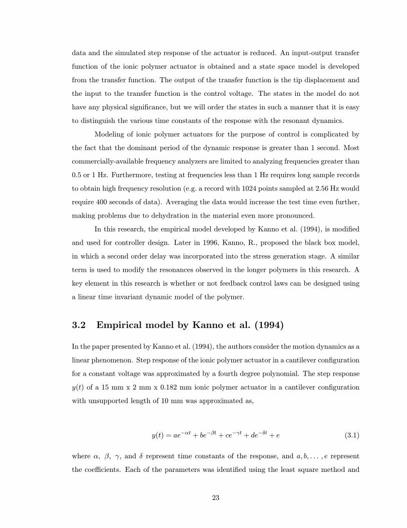
3.2 Empirical model by Kanno et al. (1994)

In the paper presented by Kanno et al. (1994), the authors consider the motion dynamics as a

linear phenomenon. Step response of the ionic polymer actuator in a cantilever configuration

for a constant voltage was approximated by a fourth degree polynomial. The step response

y(t) of a 15 mm x 2 mm x 0.182 mm ionic polymer actuator in a cantilever configuration

with unsupported length of 10 mm was approximated as,

y(t) = ae−αt + be−βt + ce−γt + de−δt + e (3.1)

where α, β, γ, and δ represent time constants of the response, and a, b, . . . , e represent

the coefficients. Each of the parameters was identified using the least square method and

23

a transfer function was developed. A table of the identified coefficients and time constants

for a range of step voltages from 0.5 Volts to 1.5 Volts was presented in this paper.

Generalizing equation (3.1), we assume that the response to the control input u(t)

is expressed in the Laplace domain as

G(s) =Y (s)

U(s)=

a

s+ α+

b

s+ β+ . . . (3.2)

In the work by Kanno, et al, the unsupported length of the ionic polymer actuator

was smaller and the response did not exhibit any contribution due to resonance. The fourth

degree transfer function was validated by observing the simulation and experimentation of

the response of the ionic polymer actuator to series of square waves (1.5 V and 0.1, 0.5, 1.5

Hz).

The empirical model presented in this work is one of the first and most useful for

a control model. However, as discussed in Chapter 2 , resonance should be given more

importance as the length of the polymer increases. In this research work, the above model

is modified to incorporate resonance and use it as a control model.

3.3 Modification of the Empirical Model

In our work, the empirical model is based on the experimental data of a series of open-loop

responses of the ionic polymer actuator to a unit step voltage. Figure 3.1a shows an open

loop response for a 26.3 mm x 5mm x 0.2mm. Figure 3.1b shows an open loop response

for a 7.8 mm x 5 mm x 0.2 mm ionic polymer actuator. The response of the long and

short polymers exhibit a fast rise time but a slow decay to steady state value. In the longer

polymers, resonance appears to be dominant in the first few seconds of the response, dying

out as the steady state value is reached, as shown in the inset in Figure 3.1a.

In this paper, equation (3.2) is modified to incorporate the resonance modes as shown

in the frequency response of the ionic polymer actuator. The model with resonant terms

can be represented in the Laplace domain as

G(s) =Y (s)

U(s)=

a

s+ α+

b

s+ β+

c

s+ γ+ · · ·+ Kr1ω

2n1

s2 + 2ζ1wn1s+ ω2n1+

Kr2ω2n2

s2 + 2ζ2wn2s+ ω2n2+ · · ·

(3.3)

24

0 2 4 6 8 10 12 14 16 18 200

20

40

60

80

100

120

140

160

180

200

220

Time (sec)

Tip

Disp

lace

men

t (m

icro

ns)

0 5 10 150

200

400

600

800

1000

1200

1400

1600

1800

2000

Tip

Disp

lace

men

t (m

icro

ns)

Time(sec)

(a) (b)

Figure 3.1: Bending response of (a) 12 mm x 5 mm x 0.2 mm actuator; (b) 40 mm x5 mm x 0.2 mm actuator.

where ωn is the natural frequency of the actuator, ζ is the nondimensional damping ratio,

and Kr represents the gain coefficient of the resonant response. The accuracy of the empir-

ical model might depend on the number of poles in the empirical model. A simpler model,

with four linear poles and a single resonance term, of equation (3.3)can be written as,

G(s) =Y (s)

U(s)=

a

s+ α+

b

s+ β+

c

s+ γ+

d

s+ δ+

Krω2n

s2 + 2ζwns+ ω2n(3.4)

3.3.1 Optimization function: FMINCON

As in the previous work by Kanno, et al, we utilize a nonlinear least squares technique to

find the optimal values of the actuator model. The optimization variables are the coefficients

a, b, . . . , the time constants α, β, . . . , and the resonant parameter terms Kr, ωn, and

ζ. The optimization is constrained to guarantee that the steady-state displacement of the

modelled response is equivalent to the measured response.

The MATLAB function FMINCON, Coleman and Zhang (2000) is used to find the

solution to the optimization problem (Mathworks, 2000). The FMINCON function finds

the constrained minimum of a scalar function of several variables starting at an initial

25

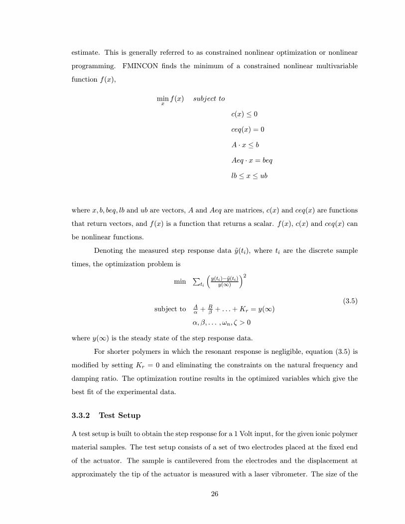
estimate. This is generally referred to as constrained nonlinear optimization or nonlinear

programming. FMINCON finds the minimum of a constrained nonlinear multivariable

function f(x),

minxf(x) subject to

c(x) ≤ 0ceq(x) = 0

A · x ≤ bAeq · x = beqlb ≤ x ≤ ub

where x, b, beq, lb and ub are vectors, A and Aeq are matrices, c(x) and ceq(x) are functions

that return vectors, and f(x) is a function that returns a scalar. f(x), c(x) and ceq(x) can

be nonlinear functions.

Denoting the measured step response data y(ti), where ti are the discrete sample

times, the optimization problem is

minPti

³y(ti)−y(ti)y(∞)

´2

subject to Aα +

Bβ + . . .+Kr = y(∞)

α, β, . . . ,ωn, ζ > 0

(3.5)

where y(∞) is the steady state of the step response data.For shorter polymers in which the resonant response is negligible, equation (3.5) is

modified by setting Kr = 0 and eliminating the constraints on the natural frequency and

damping ratio. The optimization routine results in the optimized variables which give the

best fit of the experimental data.

3.3.2 Test Setup

A test setup is built to obtain the step response for a 1 Volt input, for the given ionic polymer

material samples. The test setup consists of a set of two electrodes placed at the fixed end

of the actuator. The sample is cantilevered from the electrodes and the displacement at

approximately the tip of the actuator is measured with a laser vibrometer. The size of the

26

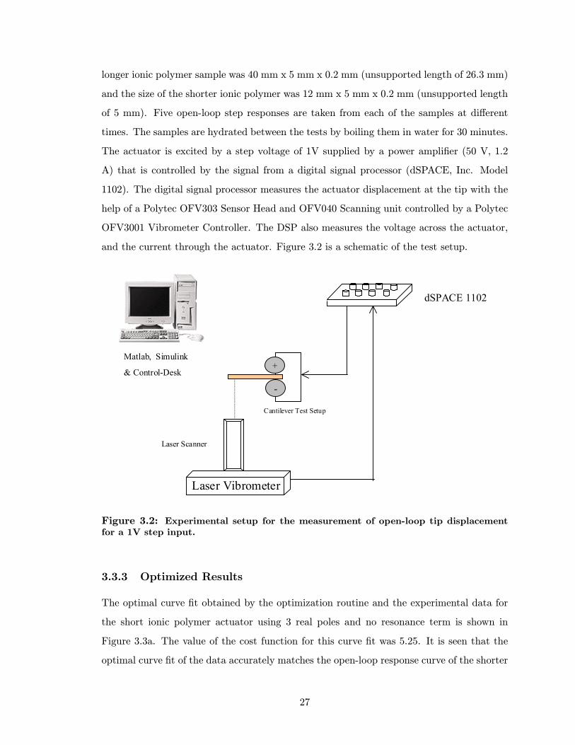
longer ionic polymer sample was 40 mm x 5 mm x 0.2 mm (unsupported length of 26.3 mm)

and the size of the shorter ionic polymer was 12 mm x 5 mm x 0.2 mm (unsupported length

of 5 mm). Five open-loop step responses are taken from each of the samples at different

times. The samples are hydrated between the tests by boiling them in water for 30 minutes.

The actuator is excited by a step voltage of 1V supplied by a power amplifier (50 V, 1.2

A) that is controlled by the signal from a digital signal processor (dSPACE, Inc. Model

1102). The digital signal processor measures the actuator displacement at the tip with the

help of a Polytec OFV303 Sensor Head and OFV040 Scanning unit controlled by a Polytec

OFV3001 Vibrometer Controller. The DSP also measures the voltage across the actuator,

and the current through the actuator. Figure 3.2 is a schematic of the test setup.

+

-

Laser Vibrometer

Matlab, Simulink

& Control-Desk

Cantilever Test Setup

Laser Scanner

dSPACE 1102

Figure 3.2: Experimental setup for the measurement of open-loop tip displacementfor a 1V step input.

3.3.3 Optimized Results

The optimal curve fit obtained by the optimization routine and the experimental data for

the short ionic polymer actuator using 3 real poles and no resonance term is shown in

Figure 3.3a. The value of the cost function for this curve fit was 5.25. It is seen that the

optimal curve fit of the data accurately matches the open-loop response curve of the shorter

27

0 2 4 6 8 10 12 14 16 18 200

20

40

60

80

100

120

140

160

180

200

220

Time (sec)

Tip

Disp

lace

men

t (m

icron

s)

0 5 10 15 20 25-500

0

500

1000

1500

2000

2500

Time (sec)

Tip

disp

lace

men

t (m

icron

s)

Experimental

OptimalExperimental

Optimized

Initial

(a) (b)

Figure 3.3: (a) Optimal curve fit using three real poles of the experimental data usingfor the 16 mm x 5 mm x 0.2 mm ionic polymer actuator sample to a 1 V step input;(b) Optimal curve fit using three real poles of the experimental data using for the 40mm x 5 mm x 0.2 mm ionic polymer actuator sample to a 1 V step input.

polymer. The optimized transfer function for the short polymer using 3 real poles of one

of the data set is shown in Equation 3.6. The optimized curve fit transfer function can be

used to develop a control model for the shorter polymers.

G(s) =Y (s)

U(s)=−0.44s+ 0.27

+802.39

s+ 69.88+−957.21s+ 108.87

(3.6)

The optimal curve fit for one of the open loop response of the longer ionic polymer

actuator using 3 real poles and one resonance term is shown in Figure 3.3b. The value

of the cost function for this curve fit was 10.71. Figure 3.3b illustrates that the optimal

curve fit of the data accurately matches the backbone of the open-loop response curve, but

does not accurately match the resonances observed. This error of model might occur due

to the FMINCON function optimization, which tries to reduce the summation of the error

at each time step. The resonant portion of the response does not contribute substantially

to the error cost function, therefore only minimal reductions in the cost function occur by

matching the response in the first 2-3 seconds of the measurement. The optimized transfer

function for the long polymer, using 3 real poles and one resonance term, of one of the data

28

set is shown in Equation 3.7.

G(s) =Y (s)

U(s)=

10.31

s+ 13.08+

6.24

s+ 0.85+−6.13s+ 0.77

+0.71(75)2

s2 + 2(0.09)(75) + (75)2(3.7)

From the optimized results of the long polymer and the short polymer shown in

this section, we can conclude that the simulation of the optimized transfer function model

adequately match the step response data obtained from experiments. Hence, the transfer

functions can be used to design a controller.

3.4 Cost Function Analysis

The curve fit obtained from the previous section shows the accuracy of the optimization

routine in obtaining an empirical model. For a more rigorous analysis of the accuracy which

can be obtained from this routine, a cost function analysis is done. The accuracy of the

curve fit routine can be varied by varying the number of variables to be optimized. For

example, the accuracy of the curve fit routine of an empirical model of long ionic polymer

actuator will vary if the model includes two real poles and two resonance terms as opposed

to a model consisting of three real poles and two resonance terms. Hence the need for a

cost function analysis arises.

The optimization variables are the coefficients a, b, . . . , the time constants α, β, . . . ,

and the resonant parameter terms Kr, ωn, and ζ. The number of variables can be altered,

by increasing or decreasing the number of poles included in an empirical model. The accu-

racy of the empirical model might depend on the number of poles in the empirical model.

The number of states in the control model is an important aspect of the design. Hence a

study of the number of the real poles required to accurately model by optimization is per-

formed by varying the number of real poles and considering one resonance term. A series

of five open loop responses for the long polymer and short polymer are optimized for three

different number of real poles in the system. The number of real poles is varied from 2 to 4.

Here it is emphasized that the cost function is square of the error of the tip displacement

of the experimental and simulated value normalized to the steady state value.

29

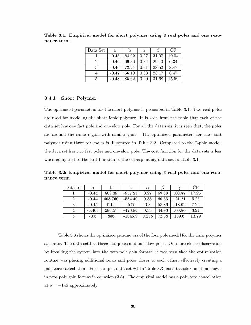
Table 3.1: Empirical model for short polymer using 2 real poles and one reso-nance term

Data Set a b α β CF

1 -0.45 84.02 0.27 31.07 19.04

2 -0.46 69.36 0.34 29.10 6.34

3 -0.46 72.24 0.31 28.52 8.47

4 -0.47 56.19 0.33 23.17 6.47

5 -0.48 85.62 0.29 31.68 15.59

3.4.1 Short Polymer

The optimized parameters for the short polymer is presented in Table 3.1. Two real poles

are used for modeling the short ionic polymer. It is seen from the table that each of the

data set has one fast pole and one slow pole. For all the data sets, it is seen that, the poles

are around the same region with similar gains. The optimized parameters for the short

polymer using three real poles is illustrated in Table 3.2. Compared to the 2-pole model,

the data set has two fast poles and one slow pole. The cost function for the data sets is less

when compared to the cost function of the corresponding data set in Table 3.1.

Table 3.2: Empirical model for short polymer using 3 real poles and one reso-nance term

Data set a b c α β γ CF

1 -0.44 802.39 -957.21 0.27 69.88 108.87 17.26

2 -0.44 408.766 -534.40 0.33 60.33 121.21 5.25

3 -0.45 421.1 -547 0.3 58.86 118.02 7.26

4 -0.466 286.57 -423.86 0.33 44.93 106.86 3.91

5 -0.5 886 -1046.9 0.288 72.38 109.6 13.79

Table 3.3 shows the optimized parameters of the four pole model for the ionic polymer

actuator. The data set has three fast poles and one slow poles. On more closer observation

by breaking the system into the zero-pole-gain format, it was seen that the optimization

routine was placing additional zeros and poles closer to each other, effectively creating a

pole-zero cancellation. For example, data set #1 in Table 3.3 has a transfer function shown

in zero-pole-gain format in equation (3.8). The empirical model has a pole-zero cancellation

at s = −148 approximately.

30

G(s) =Y (s)

U(s)=

12247(s+ 147.41)(s− 122.76)(s+ 0.10)(s+ 148.21)(s+ 115.11)(s+ 56.36)(s+ 0.27)

(3.8)

Table 3.3: Empirical model for short polymer using 4 real poles and one reso-nance term

Data set a b c d α β γ δ CF

1 -0.44 358 -147.2 -352.67 0.27 56.36 115.11 148.21 17.314

2 -0.44 355 -148 -353.2 0.33 58.39 113.49 145.82 5.25

3 -0.45 355 -148 -353 0.3 56.6 113.06 145.09 7.26

4 -0.46 354 -139 -335 0.33 47.19 85.25 97 3.87

5 -0.47 359 -166 -375 0.28 58.104 147.9 158.2 13.83

For all the above three cases, on visual inspection it was seen that the simulated

step response of the empirical model matched the experimental step response. The average

cost function of the data sets for each case is presented in Table 3.4. The cost function

represents the square of the error between the measured response and the model response

normalized to the steady state value of the response. As shown in Table 3.4, increasing the

number of real poles beyond 3 does not provide a substantial increase in model accuracy.

Table 3.4: Average cost function as number of real poles vary for short polymer

Number of real poles Average Cost Function

2 11.182

3 9.49

4 9.4

3.4.2 Long Polymer

The long polymer is optimized using two real poles and a single resonance term, whose

parameters are presented in Table 3.5. The data set has one fast pole and one slow pole.

The damping coefficient is around 0.05. On visual inspection, the resonance data did

not match very well in the the long polymers using the two pole model. The damping

coefficient varies from 0.03 to 0.15 and the natural frequency varies around 72-80 rad/sec

in the simulated empirical model.

31

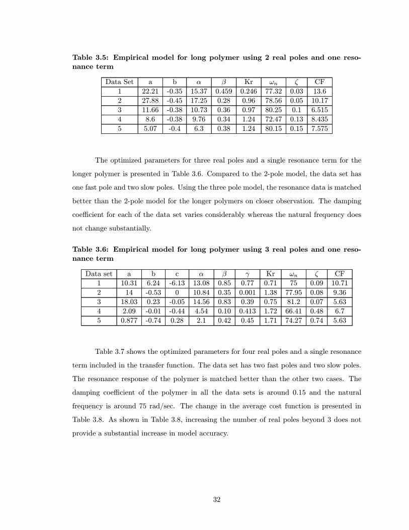
Table 3.5: Empirical model for long polymer using 2 real poles and one reso-nance term

Data Set a b α β Kr ωn ζ CF

1 22.21 -0.35 15.37 0.459 0.246 77.32 0.03 13.6

2 27.88 -0.45 17.25 0.28 0.96 78.56 0.05 10.17

3 11.66 -0.38 10.73 0.36 0.97 80.25 0.1 6.515

4 8.6 -0.38 9.76 0.34 1.24 72.47 0.13 8.435

5 5.07 -0.4 6.3 0.38 1.24 80.15 0.15 7.575

The optimized parameters for three real poles and a single resonance term for the

longer polymer is presented in Table 3.6. Compared to the 2-pole model, the data set has

one fast pole and two slow poles. Using the three pole model, the resonance data is matched

better than the 2-pole model for the longer polymers on closer observation. The damping

coefficient for each of the data set varies considerably whereas the natural frequency does

not change substantially.

Table 3.6: Empirical model for long polymer using 3 real poles and one reso-nance term

Data set a b c α β γ Kr ωn ζ CF

1 10.31 6.24 -6.13 13.08 0.85 0.77 0.71 75 0.09 10.71

2 14 -0.53 0 10.84 0.35 0.001 1.38 77.95 0.08 9.36

3 18.03 0.23 -0.05 14.56 0.83 0.39 0.75 81.2 0.07 5.63

4 2.09 -0.01 -0.44 4.54 0.10 0.413 1.72 66.41 0.48 6.7

5 0.877 -0.74 0.28 2.1 0.42 0.45 1.71 74.27 0.74 5.63

Table 3.7 shows the optimized parameters for four real poles and a single resonance

term included in the transfer function. The data set has two fast poles and two slow poles.

The resonance response of the polymer is matched better than the other two cases. The

damping coefficient of the polymer in all the data sets is around 0.15 and the natural

frequency is around 75 rad/sec. The change in the average cost function is presented in

Table 3.8. As shown in Table 3.8, increasing the number of real poles beyond 3 does not

provide a substantial increase in model accuracy.

32

Table 3.7: Empirical model for long polymer using 4 real poles and one reso-nance term

Data set a b c d α β γ δ

1 4.09 2.1 0.44 -2.46 8.28 0.92 0.91 0.73

2 560.76 -0.42 2442.67 -2806 48.16 0.28 144.72 99.34

3 -143.66 -0.35 -748 94.21 60.8 0.3 2584 28

4 48 -0.37 -25274 -64.3 22.5 0.34 49823 84

5 77.3 -0.6 0.28 42.8 31.6 0.4 0.653 75.62

Data set Kr ωn ζ CF

1 1.01 71.6 0.20 12.24

2 2.29 77.73 0.12 6.83

3 1.3 80 0.12 5.60

4 1.25 73.83 0.11 6.34

5 1.22 74.21 0.13 4.42

Table 3.8: Average cost function as number of real poles vary for longer polymer

Number of real poles Average Cost Function

2 9.07

3 8.1

4 7.75

3.4.3 Conclusions about the Cost Analysis

Cost function analysis was done for the shorter polymer and the longer polymer using one

resonance term and varying the number of real poles to model the system from 2 to 4. As

the number of real poles were increased in the short polymer model, there was no substantial

increase in accuracy when observed visually. In the longer polymer, as the number of poles

was increased, the resonance part of the response was modeled more accurately. It was

also seen that as the number of poles increased in the short polymer and the long polymer,

a pole-zero cancellation was propogating through the optimization method. Hence, by

increasing the number of real poles in the ionic polymer model, a pole zero cancellation

appears instead of an substantial increase in the accuracy. The pole-zero cancellation effect

observed, results in an unstable system with a stable transfer function [Friedland (1986)].

The transfer function is of lower order than the system and the unstable modes are either

33

not capable of being affected by the input or not visible in the output, i.e. not completely

observable and not completely controllable, which was proved by R.E. Kalman in 1950s.

This unrealistic increase of poles increases the complexity of the controller design. The cost

function analysis presented is one of the methods to prevent such effects to creep into the

empirical model.

Figure 3.4a shows the cost function variation for each of the data set optimized in a

short polymer, while Figure 3.4b shows the variation for the long polymer. It is seen that

the cost function saturates as the number of real poles is increased from 3 to 4.

2 3 42

4

6

8

10

12

14

16

18

20

No. of Real Poles

Cos

t Fun

ctio

n

2 3 44

5

6

7

8

9

10

11

12

13

14

No. of Real Poles

Cos

t Fu

nctio

n

(a) (b)

Figure 3.4: (a) Cost function variation for short polymers as number of real polesvary; (b) Cost function variation for long polymers as number of real poles vary.

34

3.5 Summary

An empirical model does not consider any physical phenomenon. In this chapter, an em-

pirical model developed by Kanno et al. (1994) was modified to incorporate resonance

behavior observed in longer polymers and was generalized for any length of ionic polymer.

Short polymers with an unsupported length of 7.8 mm do not exhibit any resonance in the

step response, hence they are modeled using 3 real poles. Longer polymers which exhibit

resonance, are modeled using 3 real poles and 2 resonant poles. This empirical model was

optimized using a function in MATLAB. The optimization results are analysed with respect

to a cost function as the number of real poles was varied for short and long polymers.

The accuracy of the model can be changed by varying the number of poles in the

model. A study of the cost function as the number of real poles are varied is done. It is seen

that as the number of real poles is varied from 3 to 4, the cost function has no substantial

decrement. Hence the empirical model developed using 3 real poles, can be used as a control

model for the ionic polymer actuator.

In this chapter, the empirical model for the ionic polymer actuator is developed

and optimized. This model can now be used for the design of a controller to increase the

bandwidth of the actuator.

35

Chapter 4

Feedback Control

The dynamic response of the ionic polymer actuator illustrates a slow settling time and

a high overshoot of the tip displacement when a step input voltage is applied. The ionic

polymer actuator has a low bandwidth due to the slow settling time observed and cannot be

used to actuate high frequency signals. Feedback control of the ionic polymer is necessary

to overcome these disadvantages.

In this chapter, the optimized transfer function from the empirical model developed

in the previous chapter is converted into a canonical state space model. A feedback controller

is designed using the Linear Quadratic Regulator (LQR) method to increase the bandwidth

of the ionic polymer actuator. Two methods of designing control systems using different cost

functions in the LQR technique are discussed for long polymers. Simulations are performed

on the closed-loop system which indicate faster settling time and a reduction in overshoot.

A perturbation analysis is discussed on the effect of the change in natural frequency on the

closed-loop stability of the system.

4.1 State Space Model

A state space model represents the dynamics of a system by a number of first-order differ-

ential equations. The optimized transfer function [Eq. (3.6) & Eq. (3.7)] is converted into a

canonical state space representation. The ionic polymer actuator is represented as a parallel

interconnection of subsystems which is advantageous for the control design. Although the

input-output relationship is independent of the state variable representation, representing

the dynamics in this form allows us to directly relate the states to the time constants of

36

the response. This is a necessary step for the LQR control used in the feedback which is

discussed in the next section.

a----------

s + a

b----------

s + b

22

2

2 nn

nr

sK

ωζωω

++

+

+

+

U(s)Y(s)

G(s)

Figure 4.1: Parallel interconnection of the control model.

The optimal values of the parameters determined from the empirical model opti-

mization are substituted into the transfer function as given by equation (3.4). A canonical

state space model of the form

x(t) = Ax(t) +Bu(t)

y(t) = Cx(t) +Du(t) (4.1)

is obtained from the optimized transfer function, where x(t) is the state vector, u(t) is the

control input, y(t) is the output (tip displacement) of the system and A, B, C, and D are

the state matrices. The system transfer function is treated as a parallel interconnection of

smaller systems as shown in Figure 4.1. Assuming this structure, equation (4.1) has the

form

37

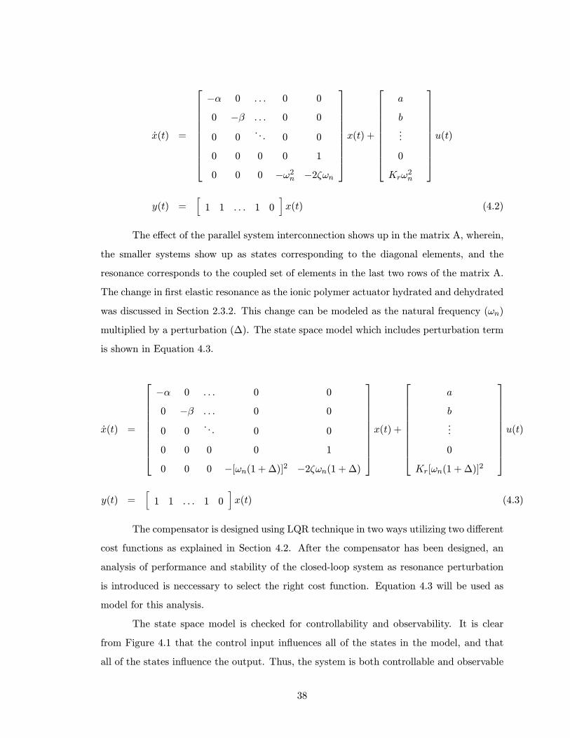
x(t) =

−α 0 . . . 0 0

0 −β . . . 0 0

0 0. . . 0 0

0 0 0 0 1

0 0 0 −ω2n −2ζωn

x(t) +

a

b...

0

Krω2n

u(t)

y(t) =h1 1 . . . 1 0

ix(t) (4.2)

The effect of the parallel system interconnection shows up in the matrix A, wherein,

the smaller systems show up as states corresponding to the diagonal elements, and the

resonance corresponds to the coupled set of elements in the last two rows of the matrix A.

The change in first elastic resonance as the ionic polymer actuator hydrated and dehydrated

was discussed in Section 2.3.2. This change can be modeled as the natural frequency (ωn)

multiplied by a perturbation (∆). The state space model which includes perturbation term

is shown in Equation 4.3.

x(t) =

−α 0 . . . 0 0

0 −β . . . 0 0

0 0. . . 0 0

0 0 0 0 1

0 0 0 −[ωn(1 +∆)]2 −2ζωn(1 +∆)

x(t) +

a

b...

0

Kr[ωn(1 +∆)]2

u(t)

y(t) =h1 1 . . . 1 0

ix(t) (4.3)

The compensator is designed using LQR technique in two ways utilizing two different

cost functions as explained in Section 4.2. After the compensator has been designed, an

analysis of performance and stability of the closed-loop system as resonance perturbation

is introduced is neccessary to select the right cost function. Equation 4.3 will be used as

model for this analysis.

The state space model is checked for controllability and observability. It is clear

from Figure 4.1 that the control input influences all of the states in the model, and that

all of the states influence the output. Thus, the system is both controllable and observable

38

indicating that the closed-loop poles can be placed anywhere in the complex plane using

full-state feedback and a linear observer.

4.2 Design of Controller

4.2.1 Linear Quadratic Regulator(LQR) Control

State-space control approaches are used to design feedback control laws for the ionic polymer

actuators using a model that consists of three real poles. Two additional resonance states

are used to model the actuator resonance for the longer polymer. To control the system,

the states are estimated by designing a linear observer-estimator as shown in Figure 4.2.

+x

A

.K

r

-^

OBSERVER

+B

C

u xx

A

.

B

y

C

+

-y^

+

-

states

stateestimates

stateerror

-Gx r

+- +

G r -

x d

F

G d

STATEFEEDBACK

FEEDFORWARDGAINS

F

+

Figure 4.2: Linear Observer-Estimator compensator to track reference inputs in statespace design.

For the design of the controller, we will utilize Linear Quadratic Regulator (LQR)

control theory to determine a set of state feedback gains. The LQR optimization produces

an optimal full-state feedback gain matrix G. It is well known that LQR control can be

used for optimizing the performance with respect to a quadratic cost function [Friedland

(1986)]. The cost function is comprised of a quadratic function of the states and a quadratic

39

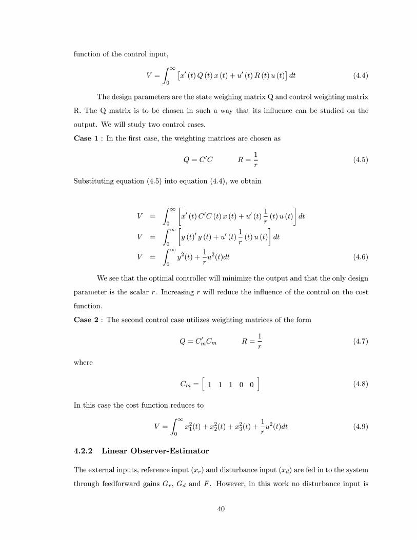
function of the control input,

V =

Z ∞0

£x0 (t)Q (t) x (t) + u0 (t)R (t)u (t)

¤dt (4.4)

The design parameters are the state weighing matrix Q and control weighting matrix

R. The Q matrix is to be chosen in such a way that its influence can be studied on the

output. We will study two control cases.

Case 1 : In the first case, the weighting matrices are chosen as

Q = C 0C R =1

r(4.5)

Substituting equation (4.5) into equation (4.4), we obtain

V =

Z ∞0

∙x0 (t)C 0C (t) x (t) + u0 (t)

1

r(t)u (t)

¸dt

V =

Z ∞0

∙y (t)0 y (t) + u0 (t)

1

r(t) u (t)

¸dt

V =

Z ∞0y2(t) +

1

ru2(t)dt (4.6)

We see that the optimal controller will minimize the output and that the only design

parameter is the scalar r. Increasing r will reduce the influence of the control on the cost

function.

Case 2 : The second control case utilizes weighting matrices of the form

Q = C 0mCm R =1

r(4.7)

where

Cm =h1 1 1 0 0

i(4.8)

In this case the cost function reduces to

V =

Z ∞0x21(t) + x

22(t) + x

23(t) +

1

ru2(t)dt (4.9)

4.2.2 Linear Observer-Estimator

The external inputs, reference input (xr) and disturbance input (xd) are fed in to the system

through feedforward gains Gr, Gd and F . However, in this work no disturbance input is

40

considered. Hence, xd = 0 & F = Gd = 0. The poles due to full-state feedback are the

eigenvalues of the matrix A− BG. The rate of convergence of the estimated states to theactual states is controlled by choosing the observer gain matrix K. The gain matrix K

is chosen by pole placement method by specifying the eigen values of the observer state

matrix A−BK. The eigenvalues of the observer state matrix A−KC are chosen to be a

multiple of two of the full-state feedback poles. This selection keeps the control gains low

and thereby maintains the control voltage across the polymer within acceptable limits while

ensuring that the observer error will converge to zero in an acceptable amount of time.

The final component of the control design is to compute a feed forward gain matrix

Gr that eliminates steady-state error. Gr is chosen to eliminate the steady state output

error due to the reference input and is computed as shown in Equation[ 4.10]. Further

details of this computation are provided in Friedland (1986).

Gr =hC (A−BG)−1B

i−1C (A−BG)−1E (4.10)

where

E =h(A−Ar) F

iSince, for a step input Ar = 0, we have E = A. Substituting the value of E in

Equation[ 4.10], we have

Gr =hC (A−BG)−1B

i−1C (A−BG)−1A (4.11)

After computing the observer gain matrix K and feed forward gain Gr, the state

space model for the observer-estimator compensator is,

˙x(t) = [A−BG−KC] x(t) +hBG−BGr K

i xr(t)y(t)

u(t) = [−G] x(t) +

hG−Gr 0

i xr(t)y(t)

(4.12)

where x(t) is the state estimate vector, xr(t) is the reference input vector and y(t) is the

output (tip displacement) of the system. Simulations of the closed-loop system are obtained

41

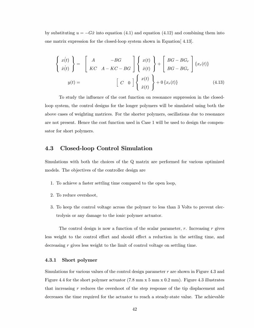
by substituting u = −Gx into equation (4.1) and equation (4.12) and combining them into

one matrix expression for the closed-loop system shown in Equation[ 4.13].

˙x(t)

˙x(t)

= A −BGKC A−KC −BG

x(t)

x(t)

+ BG−BGrBG−BGr

xr(t)y(t) =

hC 0

i x(t)

x(t)

+ 0 xr(t) (4.13)

To study the influence of the cost function on resonance suppression in the closed-

loop system, the control designs for the longer polymers will be simulated using both the

above cases of weighting matrices. For the shorter polymers, oscillations due to resonance

are not present. Hence the cost function used in Case 1 will be used to design the compen-

sator for short polymers.

4.3 Closed-loop Control Simulation

Simulations with both the choices of the Q matrix are performed for various optimized

models. The objectives of the controller design are

1. To achieve a faster settling time compared to the open loop,

2. To reduce overshoot,

3. To keep the control voltage across the polymer to less than 3 Volts to prevent elec-

trolysis or any damage to the ionic polymer actuator.

The control design is now a function of the scalar parameter, r. Increasing r gives

less weight to the control effort and should effect a reduction in the settling time, and

decreasing r gives less weight to the limit of control voltage on settling time.

4.3.1 Short polymer

Simulations for various values of the control design parameter r are shown in Figure 4.3 and

Figure 4.4 for the short polymer actuator (7.8 mm x 5 mm x 0.2 mm). Figure 4.3 illustrates

that increasing r reduces the overshoot of the step response of the tip displacement and

decreases the time required for the actuator to reach a steady-state value. The achievable

42

settling time is limited by the maximum control input objective. High values of r exhibit

a faster settling time, but increases the gains leading to an increase in initial control input.

Figure 4.4 illustrates the control input required to the polymer as a function of r.

The simulations indicate that the closed-loop control signal consists of a large initial

input followed by a slow increase in the voltage to a steady-state value. We hypothesize that

the slow voltage increase is required to offset the relaxation of the polymer. Kanno et al.

(1996b) and Newbury and Leo (2001) has measured the current variation for a step input

of a open-loop ionic polymer actuator which shows the capacitive nature of the actuator.

For a capacitor, the rate of change of voltage is proportional to the current flowing in the

capacitor. Due to the capacitive nature of the actuator, we believe that this slow voltage

rise will have a constant gradient and hence will result in a constant current across the

polymer.

0 2 4 6 8 10 12 14 16 18 20020406080

100120140160180200220

Time(sec)

Tip

Dis

plac

emen

t (m

icro

ns)

r=10-4

r=10-3

r=10-2

Open Loop

Figure 4.3: Simulation of closed-loop tip displacment of the 7.8 mm-long polymer forvarying values of the control design parameter r.

The control simulations demonstrate that the response time of the actuator can be

significantly increased with feedback control. The large overshoot and slow relaxation of

the actuator is eliminated by feedback control that utilizes tip displacement as the sensor

signal and voltage as the control signal. Table 4.1 shows the trade-off between maximum

control input and settling time as a function of the design parameter r. The simulations

43

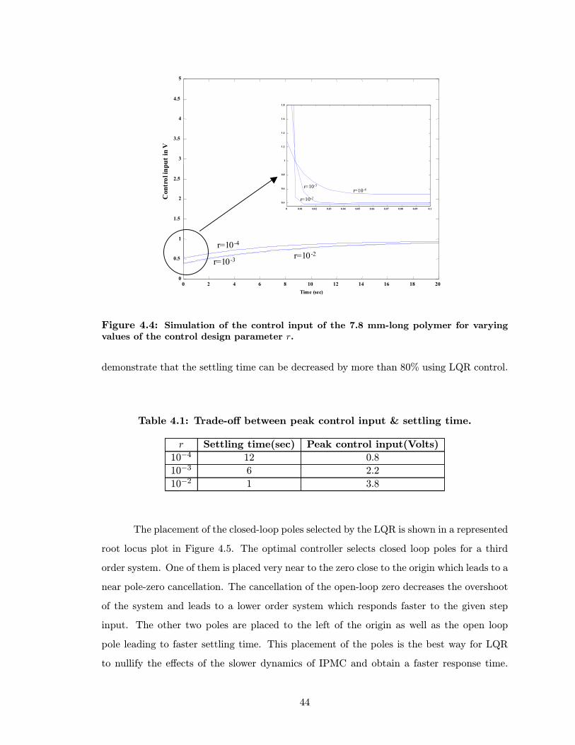
0 2 4 6 8 10 12 14 16 18 200

0.5

1

1.5

2

2.5

3

3.5

4

4.5

5

Time (sec)

Con

trol

inpu

t in

V

r=10-4

r=10-2r=10-3

0 0.01 0.02 0.03 0.04 0.05 0.06 0.07 0.08 0.09 0.1

0.4

0.6

0.8

1

1.2

1.4

1.6

1.8

r=10-4r=10-3

r=10-2

Figure 4.4: Simulation of the control input of the 7.8 mm-long polymer for varyingvalues of the control design parameter r.

demonstrate that the settling time can be decreased by more than 80% using LQR control.

Table 4.1: Trade-off between peak control input & settling time.

r Settling time(sec) Peak control input(Volts)

10−4 12 0.8

10−3 6 2.2

10−2 1 3.8

The placement of the closed-loop poles selected by the LQR is shown in a represented

root locus plot in Figure 4.5. The optimal controller selects closed loop poles for a third

order system. One of them is placed very near to the zero close to the origin which leads to a

near pole-zero cancellation. The cancellation of the open-loop zero decreases the overshoot

of the system and leads to a lower order system which responds faster to the given step

input. The other two poles are placed to the left of the origin as well as the open loop

pole leading to faster settling time. This placement of the poles is the best way for LQR

to nullify the effects of the slower dynamics of IPMC and obtain a faster response time.

44

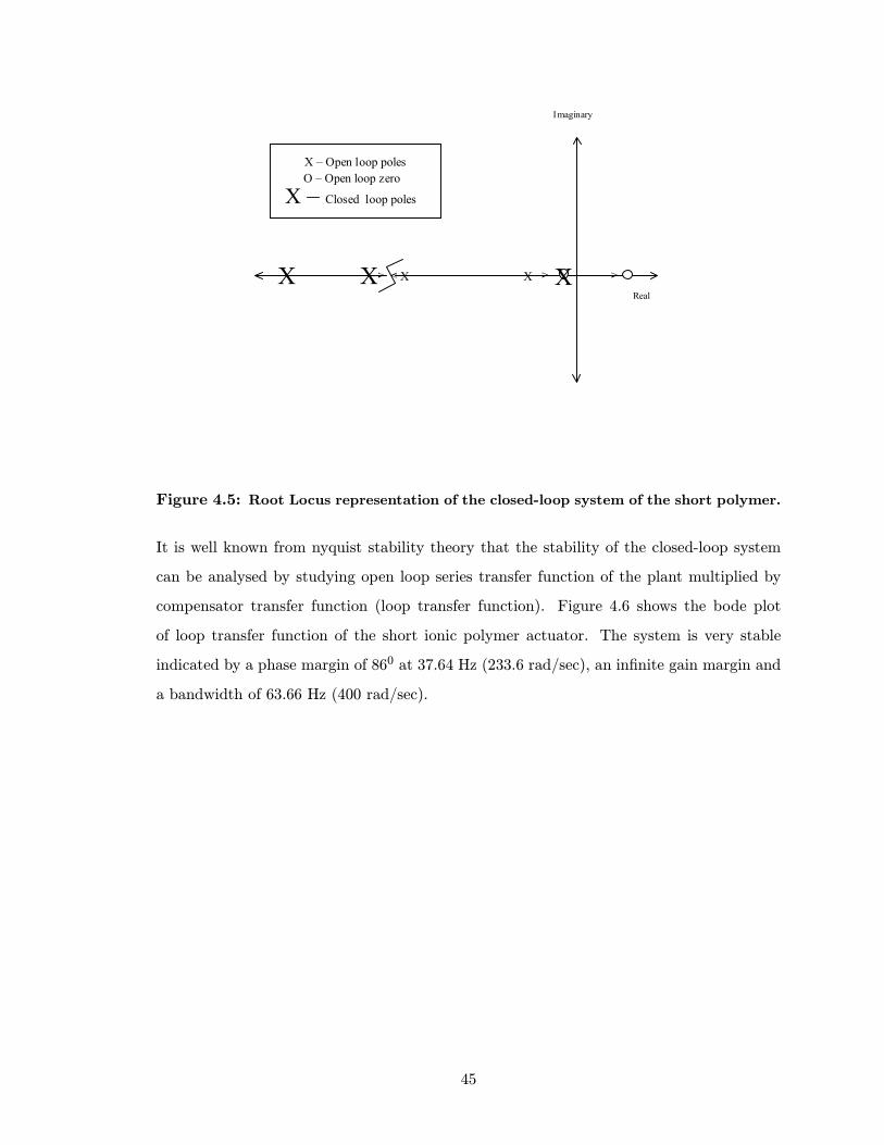
XXXX XReal

Imaginary

X – Open loop poles

X – Closed loop poles

O – Open loop zero

vv v v

Figure 4.5: Root Locus representation of the closed-loop system of the short polymer.

It is well known from nyquist stability theory that the stability of the closed-loop system

can be analysed by studying open loop series transfer function of the plant multiplied by

compensator transfer function (loop transfer function). Figure 4.6 shows the bode plot

of loop transfer function of the short ionic polymer actuator. The system is very stable

indicated by a phase margin of 860 at 37.64 Hz (233.6 rad/sec), an infinite gain margin and

a bandwidth of 63.66 Hz (400 rad/sec).

45

10-3

10-2

10-1

100

101

102

103

10-2

100

102

Frequency (Hz)

Mag

nitu

de (m

icron

s/V)

10-3

10-2

10-1

100

101

102

103

-200

-150

-100

-50

0

50

Frequency (Hz)

Phas

e (de

g)

PM = 860

Figure 4.6: Bode plot of the closed loop system of the short polymer.

46

4.3.2 Case 1: Long polymer - Resonance term included in Q

A second series of control simulations are performed for the model of the 26.3 mm-long ionic

polymer actuator using a control design that incorporates the resonance terms in the LQR

cost function (i.e. Q = C 0C). Figure 4.7 illustrates that control system provides reduction of

the settling time as the r factor is increased. The reduction in settling time is accompanied

by a decrease in the oscillatory response of the polymer in the first 2-3 seconds of the step

response. The control input for the simulation cases are shown in Figure 4.8. The control

signal for this case has the same characteristics as the control signal for the short polymer

(Figure 4.4), but exhibits a oscillatory response in the first 2 seconds to nullify the effects

of the resonance (see the inset of Figure 4.8).

Time(sec)

0 5 10 150

500

1000

1500

2000

Tip

Disp

lace

men

t (m

icro

ns) Open Loop

r=10-6

r=10-4

r=10-5

Figure 4.7: Simulation of the tip displacement for the 26.3 mm long polymer withweighting matrix Q = C 0C.

The low frequency oscillations seen in the open-loop data of the step response are

now reduced considerably by using the controller in the closed-loop system. Hence, time

response simulations indicate that feedback control is eliminating the effects of resonance

in the response of the polymer actuator. This is investigated in more detail by examining

the frequency response functions of the plant, compensator, and the system defined by the

series combination of the plant and compensator. Figure 4.9a is the frequency response of

47

0 5 10 150

0.5

1

1.5

2

2.5

3

3.5

Time (sec)

Con

trol

inpu

t in

V

r = 10-5

r = 10-6

r = 10-7

r = 10-7

r = 10-6

r = 10-5

Figure 4.8: Simulation of the control input for the 26.3 mm long polymer with weight-ing matrix Q = C 0C.

the plant illustrating the low frequency dynamics associated with the time constants α, β,

and γ, and the magnitude and phase changes associated with the resonant terms in the 10-

20 Hz frequency range. The resonant frequency is approximately at 13 Hz for this actuator

at the time of experiment. Figure 4.9b is the bode plot of the compensator and the system,

which illustrates that the LQR controller is a lead compensator that adds phase near the

resonance frequency of the actuator. Lead compensation increases the phase margin and

provides closed-loop damping to the actuator resonance.

Examining the closed loop poles selected by the LQR, we see a very interesting

result. The optimal controller selects closed loop poles for a fifth order system, as shown

in Figure 4.10. Three of them are placed near to the zeros which leads to a near pole-zero

cancellation. The cancellation of the open-loop zero decreases the overshoot of the system

and makes the response faster to the step input. The set of resonance poles are placed

diagonally far from the open loop resonance poles to the left of the s-plane leading to faster

settling time. Hence the closed-loop resonance poles are placed at a higher damping ratio

than the open-loop resonance poles, increasing the settling time. LQR minimizes the effect

of resonance in the longer polymers and leads to a faster settling time with less overshoot

with this placement of the poles. Figure 4.11 shows the bode plot of the series connection of

48

10-2

10-1

100

101

102

101

102

103

104

Frequency (Hz)

Mag

nitu

de (m

icron

s/V)

10-2

10-1

100

101

102

-200

-150

-100

-50

0

50

Frequency (Hz)

Phas

e (de

g)

10-2

10-1

100

101

102

10-4

10-2

100

102

Frequency (Hz)

Mag

nitu

de (m

icron

s/V)

10-2

10-1

100

101

102

-200

-150

-100

-50

0

Frequency (Hz)

Phas

e (de

g)

Compensator

Compensator

System

System

(a) (b)

Figure 4.9: (a) Transfer function of the actuator at the time of the experiment; (b)Bode plot of the compensator and the system for Q = C 0C.

actuator and compensator of long ionic polymer actuator for Case 1. The system is stable

and gives satisfactory performance which is indicated by a phase margin of 460 at 27.5 Hz

(174 rad/sec), a high gain margin of 15.7 dB at 80 Hz (498 rad/sec) and a bandwidth of

33.42 Hz (210 rad/sec).

49

XXXReal

Imaginary

X – Open loop poles

X – Closed loop poles

O – Open loop zero

X X X

X

X

X

X

vv v vFigure 4.10: Root Locus representation of the closed-loop system of the long polymerfor Case 1.

10-3

10-2

10-1

100

101

102

10-2

100

102

Frequency (Hz)

Mag

nitu

de (m

icron

s/V)

10-3

10-2

10-1

100

101

102

-200

-150

-100

-50

0

50

Frequency (Hz)

Phas

e (de

g)

PM = 460

GM = 15dB

Figure 4.11: Bode plot of the series plant and compensator of the long polymer forCase 1.

50

4.3.3 Case 2: Long Polymer - Resonance term ignored in Q

A final series of control simulations are performed using the weighting matrix Q = C 0mCm.

Figure 4.12a shows a change in the settling time as the r factor is increased. The primary

difference between the controlled response for this weighting matrix and the weighting

matrix for Case 1 is that the closed-loop response still exhibits oscillation in the first 2-3

seconds after the step is applied. Figure 4.12b shows the increase in the control input as the

r factor is increased. The rationale for this time response is examined by investigating the

frequency response of the compensator and system. Figures 4.13a and b are the Bode plots

for the plant, compensator, and system. Figure 4.13b illustrates that the compensator is

adding a notch at the resonant frequency of the plant. The settling time does not change

as much as the previous case due to the rolloff at higher frequencies, but the notch in the

compensator does not provide the phase lead as in the case of the design that utilized

Q = C 0C as the state weighting matrix. Due to this, the bandwidth is limited and the

controlled response still exhibits the oscillations associated with resonance of the actuator.

0 5 10 150

200

400

600

800

1000

1200

1400

1600

1800

2000

Time(sec)

Tip

Dis

pla

cem

ent

(mic

rons

)

Open Loop

r=10-4

r=10-5

r=10-6

0 5 10 15 20 25 300.2

0.4

0.6

0.8

1

1.2

1.4

1.6

1.8

Time (sec)

Con

trol

inp

ut

in V

r = 10-5

r = 10-4

r = 10-6

Figure 4.12: (a) Simulation of the tip displacement for the 40 mm-long polymer forQ = C 0mCm; (b)Simulation of the control input.

In both the above cases, the slope of the control voltage input decreases as time

progresses during settling. The reason for this behavior can be explained by the nature

51

10-2

100

102

100

102

104

Mag

nitu

de (m

icron

s/V)

10-2

100

102

-200

-100

0

Phas

e (de

g)

10-2

100

102

100

Mag

nitu

de (

mu/

V)

10-2

100

102

-200

0

200

400

Phas

e (de

g)

frequency (Hz) frequency (Hz)

(a) (b)

System

Compensator

System

Compensator

Figure 4.13: (a) Bode plot of the plant; (b) Bode plot of the compensator and systemfor Q = C 0mCm.

of the ionic polymer actuator to behave largely as a capacitor. In the absence of feedback

control, the current through the actuator increases rapidly and then decreases exponentially

to zero (Kanno, R., 1994) when a step voltage is applied. After this rapid increase, the

current through the ionic polymer actuator does not decrease exponentially to zero as in

the open loop. The control voltage has a gradual slope during the settling. This shows that

current is still flowing through the ionic polymer actuator and its slope also varies until the

control voltage is steady. Taking the physical phenomenon into account as predicted by

plausible models suggested by others, we can deduce that the current is flowing across the

polymer to oppose the back diffusion of the water in the ionic polymer actuator.

Examining the closed loop poles selected by the LQR, we see a classic example of

pole-zero cancellation. As shown in Figure 4.14, the cancellation takes place at the four

locations on the s-plane. The open-loop resonance poles are cancelled by placing a closed-

loop zero. Two sets of pole-zero cancellation are introduced by the compensator at two

locations on the real axis. Compared to the other cases, the open loop zero very close to

the origin is not cancelled. Hence overshoot in the system and the response to the step

input do not change adequately. A set of resonance poles are placed diagonally far from

the open loop resonance poles to the left of the s-plane. Figure 4.15 shows the bode plot of

52

XXXReal

Imaginary

X X

X

X

X

X – Open loop poles

X – Closed loop poles

O – Open loop zero

O – Closed loop zeros

O

XO O

OXOo

Xv vv

Figure 4.14: Root Locus representation of the closed-loop system of the long polymerfor Case 2.

the series connection of actuator and compensator of long ionic polymer actuator for Case

2. The system is very close to being unstable. The bode plot illustrates the proximity to

unstability by a phase margin of 53.90 at 13.37 Hz (83.8 rad/sec), a very low gain margin

of 4.3dB at 27.5 Hz (173 rad/sec).

53

10-3

10-2

10-1

100

101

102

10-4

10-2

100

Frequency (Hz)

Mag

nitu

de (m

icron

s/V)

10-3

10-2

10-1

100

101

102

-250

-200

-150

-100

Frequency (Hz)

Phas

e (de

g)

PM =540

Figure 4.15: Bode plot of the series plant and compensator of the long polymer forCase 2.

54

4.3.4 Simulations with Perturbation

At the end of Section 4.1, perturbation variable (∆) was introduced to model the changes

in the natural frequency (ωn) of the ionic polymer actuator. The stability of the closed-

loop system of the long ionic polymer actuator is analyzed by simulating the system with

perturbation for both of the above discussed cost functions.

Case 1: Resonance term included in Q

Figure 4.16 shows the simulation of the tip displacement for r = 10−4 for a perturba-

tion factor of 9%, in which the resonant frequency of the ionic polymer plant is changed from

13 Hz to 14.2 Hz. The settling time to steady state increases to 3.2 seconds as compared to

the zero-perturbation settling time. The bode plot shown in Figure 4.17 illustrates that the

phase margin of 420 does not change substantially from the zero perturbation phase margin

of 460 and the gain margin still remains high. The stability of this system illustrates that

the cost function used in the design of the compensator is robust for perturbation in the

resonant frequency.

0 5 10 15 20 25 300

200

400

600

800

1000

1200

1400

1600

1800

2000

Time(sec)

Tip

Dis

plac

emen

t (m

icro

ns)

Figure 4.16: Tip displacement of the long polymer actuator for a perturbation factorof 9% in Case 1.

55

10-3

10-2

10-1

100

101

102

103

10-5

100

Frequency (Hz)

Mag

nitu

de (m

u/V

)

10-3

10-2

10-1

100

101

102

103

-200

-150

-100

-50

0

50

Frequency (Hz)

Phas

e (de

g)

Figure 4.17: Bode plot of the series plant and compensator of the long polymer for aperturbation factor of 9% in Case 1.

56

Case 2: Resonance term not included in Q

0 0.5 1 1.5 2 2.5 3 3.5

-6

-4

-2

0

2

4

6

x 1025

Time (sec)

Tip

Disp

lace

men

t (m

icor

ns)

Figure 4.18: Tip displacement of the long polymer actuator for a perturbation factorof 9% for case 2.

Figure 4.18 shows the simulation of the tip displacement for r = 10−4 for a pertur-

bation factor of 9%, in which the resonant frequency changed from 12 Hz to 14 Hz. The

system is unstable. The bode plot shown in Figure 4.19 illustrates that the closed-loop is

unstable since the phase margin and the gain margin are zero. The proximity to instability

in the system to a change in natural frequency of the plant by 9% proves that the cost func-

tion used for the design of the compensator is not preferred if perturbation in the resonant

frequency occurs.

The variation of the ratio of the settling time with perturbation to the settling time

without perturbation as the perturbation factor ∆ varies, is shown in Figure 4.20. In case

1, The settling time of the polymer increases as ∆→ −0.3. Similarly, the settling time alsoincreases as ∆→ +0.3. However, the system is stable for −0.3 < ∆ < 0.3 for case 1.

In contrast, in case 2, the settling time of the polymer does not change much as

∆ → −0.3. This can be explained as the compensator has a low gain margin at lower

frequencies. Hence, at the resonant frequency of the ionic polymer, the magnitude of the

compensator times the plant is very low, which does not affect the stability of the system.

However, the closed-loop system of the polymer goes unstable as ∆ → +0.3. This is due

57

10-3

10-2

10-1

100

101

102

10-2

10-1

100

101

Frequency (Hz)

Mag

nitu

de (m

icron

s/V)

10-3

10-2

10-1

100

101

102

-240

-220

-200

-180

-160

Frequency (Hz)

Phas

e (de

g)

GM = 0 dB, PM = 0 (Unstable Closed Loop)

Figure 4.19: Bode plot of the series plant and compensator of the long polymer for aperturbation factor of 9% in Case 2.

to the increase in gain margin of the compensator after the resonant frequency, which adds

up to the resonance phenomenon of the plant. Figure 4.21 shows that system for case 2,

where Q = C 0mCm goes unstable at ∆ = 0.08.

58

-0.3 -0.2 -0.1 0 0.1 0.2 0.30

50

100

150

200

250

300

350

400

Tss/

To Q=C’C

Q=Cm’Cm

Q=C’CQ=Cm’Cm

Delta D

Figure 4.20: Variation of the Settling Time ratio as Pertubation changes(−0.3 < ∆ <0.3).

-0.1 0-5

0

5

10

15

20

25

30

35

Delta D

Tss/

To

Q=Cm’Cm

Q=C’C

0.1

Figure 4.21: Variation of the Settling Time ratio as Pertubation changes (−0.1 < ∆ <0.1).

59

4.4 Summary

In this chapter, the empirical model developed in the previous chapter was converted into

a canonical state space model. The ionic polymer actuator was modeled as a parallel inter-

connection of subsystems representing single time constants and resonance. A perturbation

factor was introduced in the state space model to study the effects of change in resonant

frequency on the design of the compensator.

The controller was designed using an observer estimator with LQR techniques. The

number of design variables was reduced to one using the LQR method selecting appropriate

cost functions. Two cost functions were used which varied in the inclusion of resonance

terms. Simulations of the closed-loop system of the short-polymer showed a fast settling

time and a high initial control input followed by a slow increase. The stability of the system

was discussed using bode plots and the placement of poles was explained using the root

locus plot. Simulations of the closed-loop system of the long polymer using cost function

including the resonance terms showed a fast settling time. Simulations of the closed-loop

system of the long polymer using cost function without including the resonance terms showed

no substantial change in the settling time. The system was close to instability which was

illustrated using bode plots and placement of poles using the root locus plot.

To study the effects of change in resonant frequency on the design of the compensator

using two different cost functions, simulations of the closed-loop system of the long polymer

were performed by varying the perturbation factor from −0.9 to +0.9. The design of thecompensator using cost function including the resonance terms was more robust compared

to the design of the compensator using the cost function which excludes the resonance

terms.

The feedback control of the ionic polymer actuator when simulated showed that the

settling time is faster when a step input is given. Using the controller, the bandwidth of

the actuators can be increased and it can be used to actuate high frequency signals.

60

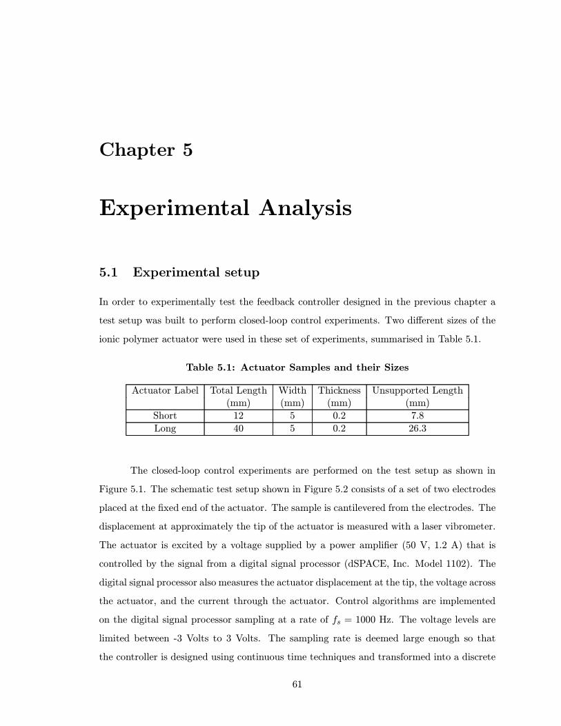
Chapter 5

Experimental Analysis

5.1 Experimental setup

In order to experimentally test the feedback controller designed in the previous chapter a

test setup was built to perform closed-loop control experiments. Two different sizes of the

ionic polymer actuator were used in these set of experiments, summarised in Table 5.1.

Table 5.1: Actuator Samples and their Sizes

Actuator Label Total Length Width Thickness Unsupported Length(mm) (mm) (mm) (mm)

Short 12 5 0.2 7.8

Long 40 5 0.2 26.3

The closed-loop control experiments are performed on the test setup as shown in

Figure 5.1. The schematic test setup shown in Figure 5.2 consists of a set of two electrodes

placed at the fixed end of the actuator. The sample is cantilevered from the electrodes. The

displacement at approximately the tip of the actuator is measured with a laser vibrometer.

The actuator is excited by a voltage supplied by a power amplifier (50 V, 1.2 A) that is

controlled by the signal from a digital signal processor (dSPACE, Inc. Model 1102). The

digital signal processor also measures the actuator displacement at the tip, the voltage across

the actuator, and the current through the actuator. Control algorithms are implemented

on the digital signal processor sampling at a rate of fs = 1000 Hz. The voltage levels are

limited between -3 Volts to 3 Volts. The sampling rate is deemed large enough so that

the controller is designed using continuous time techniques and transformed into a discrete

61

compensator using a Tustin transformation. Also, the limited frequency content of the

input signal (i.e. the step excitation) is such that no anti-aliasing filters are required. In

the continuous domain, the state space model of the compensator equations are given in

Equation[ 5.1].

˙x(t) = (A−BG−KC) x(t) +hBG−BGr K

i xr(t)

y(t)

u(t) = −Gx(t) +

hG−Gr 0

i xr(t)

y(t)

(5.1)

The continuous state space model is converted into a discretised model by Convert

to discrete time using the bilinear (Tustin) approximation to the derivative using the C2DM

function provided in MATLAB. In the Tustin method, the continuous s-domain is mapped

on to the discretized z-domain using the transformation shown in Equation[ 5.2].

s← 2fsz − 1z + 1

(5.2)

Figure 5.1: Experimental setup for closed-loop control

62

+

-

Laser Vibrometer

Matlab, Simulink

& Control-Desk

Cantilever Test Setup

Laser Scanner

dSPACE 1102

Figure 5.2: Schematic of the experimental setup for closed-loop control

5.2 Experimental Results

5.2.1 Short Polymer

A plot of the tip deflection as a function of time for the shorter polymer in an open-loop

and closed-loop is shown in Figure 5.3. The plots have been normalized by their steady-

state value to emphasize the difference in settling time and overshoot. The steady-state

value for the plot is on the order of 150 µm and can be varied by changing the value of

the step input to the control system. As predicted by the simulations, feedback control

reduces the overshoot and settling time of the tip deflection. The overshoot of the response

is reduced from 500% (5:1) to approximately 30% (1.3:1). The settling time is reduced from

approximately 13 seconds to between 3 and 4 seconds.

Experimental measurements of the tip displacement, as the values of the gain applied

practically are varied, is shown in Figure 5.4. It is observed that as the value of the control

design parameter r increased, the settling time is faster.

It is observed that as the value of the control design parameter r increased beyond

r = 10−3, the system became unstable. As r increases beyond a certain value, the initial

control input becomes very high. The system is more sensitive to this sudden spike in the

63

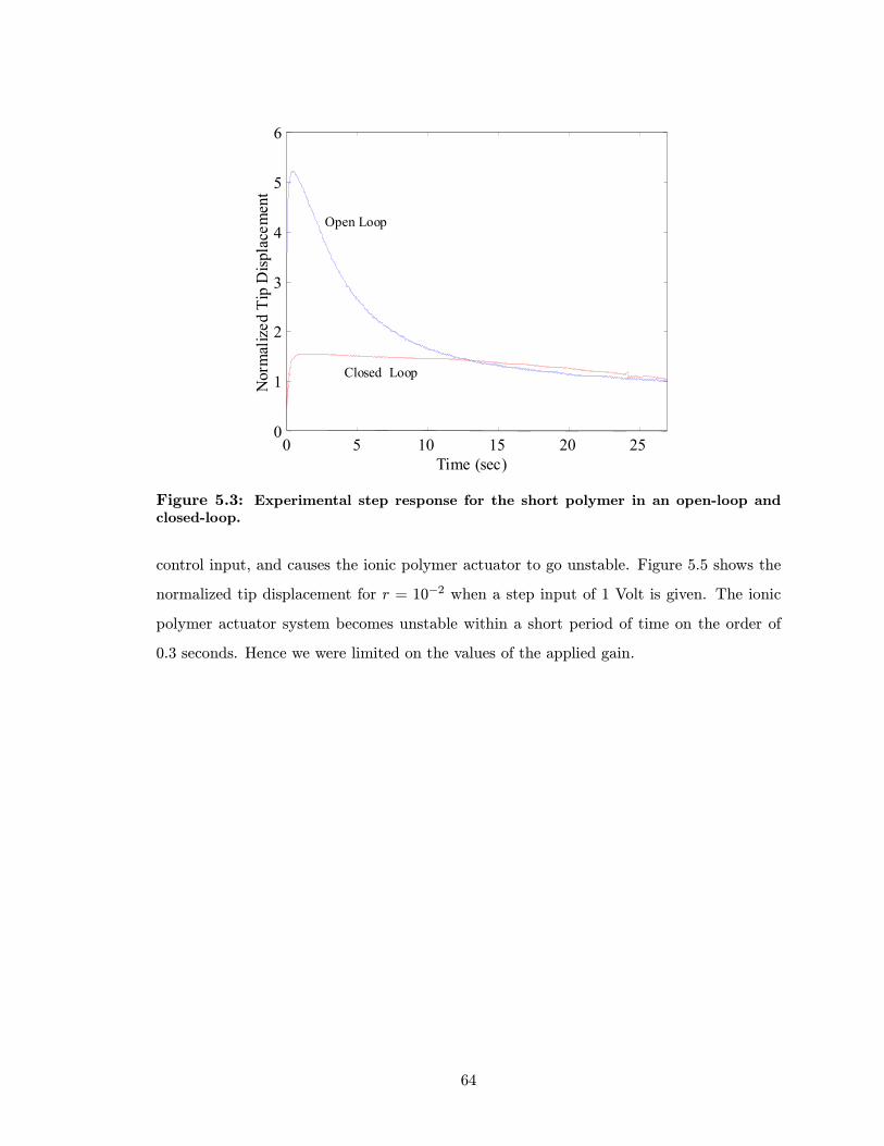
0 5 10 15 20 250

1

2

3

4

5

6

Time (sec)

Nor

mal

ized

Tip

Disp

lace

men

t

Open Loop

Closed Loop

Figure 5.3: Experimental step response for the short polymer in an open-loop andclosed-loop.

control input, and causes the ionic polymer actuator to go unstable. Figure 5.5 shows the

normalized tip displacement for r = 10−2 when a step input of 1 Volt is given. The ionic

polymer actuator system becomes unstable within a short period of time on the order of

0.3 seconds. Hence we were limited on the values of the applied gain.

64

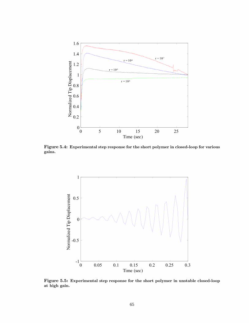
0 5 10 15 20 250

0.2

0.4

0.6

0.8

1

1.2

1.4

1.6

Time (sec)

Nor

mal

ized

Tip

Disp

lace

men

t r = 10-7r = 10-6

r = 10-4

r = 10-5

Figure 5.4: Experimental step response for the short polymer in closed-loop for variousgains.

0 0.05 0.1 0.15 0.2 0.25 0.3-1

-0.5

0

0.5

1

Time (sec)

Nor

mal

ized

Tip

Disp

lace

men

t

Figure 5.5: Experimental step response for the short polymer in unstable closed-loopat high gain.

65

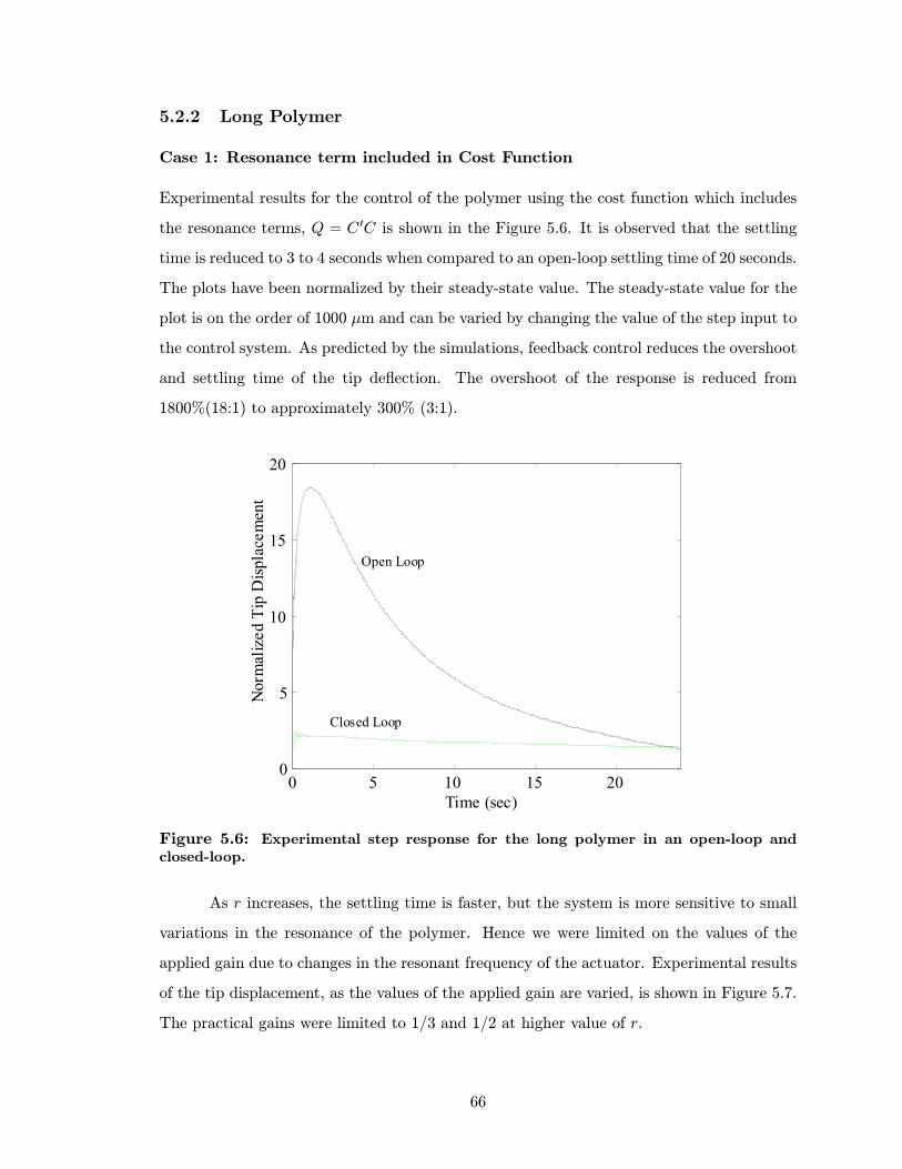
5.2.2 Long Polymer

Case 1: Resonance term included in Cost Function

Experimental results for the control of the polymer using the cost function which includes

the resonance terms, Q = C 0C is shown in the Figure 5.6. It is observed that the settling

time is reduced to 3 to 4 seconds when compared to an open-loop settling time of 20 seconds.

The plots have been normalized by their steady-state value. The steady-state value for the

plot is on the order of 1000 µm and can be varied by changing the value of the step input to

the control system. As predicted by the simulations, feedback control reduces the overshoot

and settling time of the tip deflection. The overshoot of the response is reduced from

1800%(18:1) to approximately 300% (3:1).

0 5 10 15 200

5

10

15

20

Time (sec)

Nor

mal

ized

Tip

Disp

lace

men

t

Open Loop

Closed Loop

Figure 5.6: Experimental step response for the long polymer in an open-loop andclosed-loop.

As r increases, the settling time is faster, but the system is more sensitive to small

variations in the resonance of the polymer. Hence we were limited on the values of the

applied gain due to changes in the resonant frequency of the actuator. Experimental results

of the tip displacement, as the values of the applied gain are varied, is shown in Figure 5.7.

The practical gains were limited to 1/3 and 1/2 at higher value of r.

66

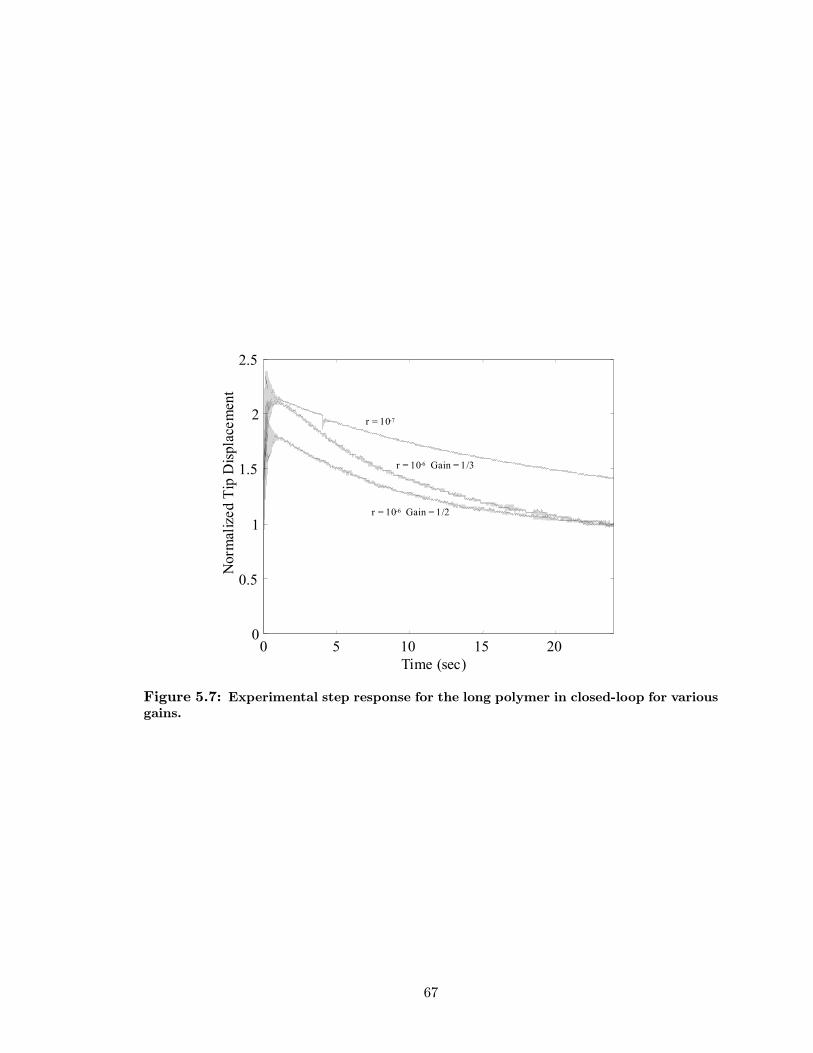
0 5 10 15 200

0.5

1

1.5

2

2.5

Time (sec)

Nor

mal

ized

Tip

Disp

lace

men

t

r = 10-6 Gain = 1/3

r = 10-7

r = 10-6 Gain = 1/2

Figure 5.7: Experimental step response for the long polymer in closed-loop for variousgains.

67

Case 2: Resonance terms not included in Cost Function

Experimental results for the control of the polymer using the cost function which does not

include the resonance terms, Q = C 0mCm is shown in the Figure 5.8. It is observed that the

settling time is reduced to 4 to 5 seconds when compared to an open-loop settling time of 25

seconds. The plots have been normalized by their steady-state value. The response for the

case Q = C 0mCm achieves a steady-state value near approximately zero tip displacement.

This is caused by the fact that the value of r for this form of the state weighting matrix

cannot be increased much beyond 10−7 due to a closed-loop instability. Any change in

the resonance frequency introduces increases in the magnitude of the system frequency

response and has the potential to cause instability in the closed loop. Figure 5.9 shows

one measurement of the tip displacement at higher gains where the system oscillates and

becomes unstable.

As predicted by the simulations, feedback control reduces the overshoot and settling

time of the tip deflection. The overshoot of the response is reduced from 1800%(18:1) to

approximately 800% (8:1).

0 5 10 15 200

5

10

15

20

Time (sec)

Nor

mal

ized

Tip

Disp

lace

men

t

Open Loop

Closed Loop

Figure 5.8: Experimental step response for the long polymer in an open-loop andclosed-loop.

Experimental results of the tip displacement, as the values of the applied gain are

68

0 5 10 15 20-1

-0.5

0

0.5

1

Time (sec)

Nor

mal

ized

Tip

Disp

lace

men

t

Figure 5.9: Unstable experimental step response for the long polymer in closed-loopfor high gain.

varied, is shown in Figure 5.10. The practical gains were as low as 1/20 and 1/12 at higher

value of r.

5.2.3 Analysis of Results

Experimental results for the short polymer illustrate that feedback control reduces the

overshoot and the settling time. By varying the magnitude of the step input, the steady

state value can be changed. For high values of the design parameter r, the closed-loop system

goes unstable. The experiments follow the simulations to a large extent and satisfactory

results are achieved by using feedback control for the short polymer when a step voltage is

given.

Experimental results for the control of the long polymer indicate that as the value

of the control design parameter r increased, the system became unstable. Although both

control systems are limited in their performance, the control system that utilizes the reso-

nant states in the weighting function (Case 1) results in much better performance than the

design that ignores the resonant states (Case 2). The response of the ionic polymer actuator

(tip displacement) for Q = C 0mCm has a settling time of 6 seconds, and Q = C 0C has a

69

0 5 10 15 200

5

10

15

20

Time (sec)

Nor

mal

ized

Tip

Disp

lace

men

tr = 10-8 Gain = 1/2

r = 10-7 Gain = 1/20

r = 10-7 Gain = 1/12

Figure 5.10: Experimental step response for the long polymer in closed-loop for variousgains.

settling time of 10 seconds as compared to the open loop settling time of 20 seconds. The

simulation shows a much faster response, but due to the limitation of the gains, the experi-

mental response does not match the simulation. An important attribute of the closed-loop

response is that the overshoot due to a step is decreased dramatically. We note that the

controlled response has an overshoot on the order of 20-30%, compared to the ratio of the

peak to steady-state value exhibited by the open-loop response.

For Case 2, the instability is attributed to test-to-test variations in the resonance

frequency and the fact that this controller is placing a notch at the resonance frequency of

the model. As shown in Figure 4.13b, ideal pole-zero cancellation eliminates the changes

in magnitude associated with the actuator resonance and enables the system to have small

phase margins and still maintain stability. In contrast, in Case 1, the control design that

utilizes Q = C 0C places lead compensation in the network to provide additional phase mar-

gin near resonance. Additional phase is a more robust method of controlling the resonance

because it is less sensitive to small variations in the natural frequency as a result of surface

dehydration or test-to-test variations in the resonance.

70

5.3 Summary

In this chapter, the feedback controller developed in the Chapter 4 is tested experimentally.

The control of short polymer showed reduction in settling time and overshoot. The system

was stable for low value of design parameter and instablity was observed at high value of

design parameter due to the initial spike of current.

The control of the longer polymer was acheived by two methods as shown in the

simulations in the previous chapter. Both the methods showed a reduction in settling time

and overshoot. In the first method, where the resonance terms were included in the cost

function, the closed-loop system was relatively stable when compared to the second method

at high value of design parameter r.

71

Chapter 6

Contributions, Conclusions,

Recommendations and Future

Work

6.1 Contributions

The following is a list of contributions made in this work:

• The step response of the ionic polymer actuator was studied in a cantilever configura-tion. The importance of control of resonance was stressed by studying the frequency

response data of three different sizes of the polymer. The change in the natural

frequency as the ionic polymer dehydrated and re-hydrated was quantified.

• An empirical model was developed and generalized for any length of the polymer.Resonance terms were included to model the resonance seen in longer polymers. The

accuracy of the empirical model as a function of the number of real poles in the model

was studied for a short and long polymers.

• A linear observer-estimator controller was designed using the LQR techniques whichreduced the settling time and the overshoot in closed-loop simulations. The response

and stability of the closed-loop system for a long ionic polymer actuator was studied

for two different cost functions.

• Experiments were conducted on the closed-loop ionic polymer actuator system. Faster

72

settling time and reduction in overshoot in the tip displacement was observed by

using feedback control. The closed-loop system of the ionic polymer actuator became

unstable at high values of the design parameter r, as predicted by the simulations,

due to the change in resonance frequency as it dehydrates during testing.

6.2 Conclusions

A test setup to measure the tip displacement of the ionic polymer actuator in a cantilever

configuration was built. From the analysis and work in this research, the following conclu-

sions are made:

• The tip displacement of an ionic polymer actuator in a cantilever configuration, toa step input of 1 Volt was studied. The dynamic response showed a fast rise time,

on the order of 0.05 seconds, and a slow settling time to steady state on the order of

5-15 seconds. High overshoot was also observed due to the ratio between the peak

response and the steady state value.

• The dynamic response for longer polymers was studied. For a step input of 1 Volt,oscillations due to resonance were observed during the first few seconds of the step

input. The variation in the stiffness of the actuators due to changes in hydration

was studied. The value of the change in the natural frequency mentioned does not

represent the entire population of samples tested since a statistical analysis was not

presented. For the five experiments performed in the dehydration test, a change

of 12.5% in the natural frequency on the first resonance was observed which was

caused due to the effect of dehydration and continual usage. For the two experiments

performed in the re-hydration test, a change of 6.6% in the natural frequency was

observed which did not match with our hypothesis that the natural frequency of the

actuator will remain the same if the material is rehydrated after a period of continual

use.

• The frequency response data for the 3 different lengths of ionic polymer actuatorsdemonstrate that control of resonance should be given more importance as the length

of the polymer increases. Difficulties in controlling the hydration and the change of

hydrations as time progresses result in mechanical inconsistency. This neccesitates

73

feedback control to improve and shape the dynamic response of the actuator and

increase the bandwidth of the actuator.

• The modeling of the ionic polymer actuator to develop a control model using phys-ical phenomenon is infeasible due to complexities involved and incomplete models

suggested. An empirical model suggested by Kanno et al. (1994) was modified to

incorporate resonance observed in long polymers and optimized using the least square

method. The simulation of such an empirical model to a step input closely matched

the experimental data obtained.

• The accuracy of the empirical model as a function of the number of real poles in themodel was studied for both short and long polymers. It was observed that increasing

the number of real poles did not substantially increase the accuracy of the model. A

pole-zero cancellation appeared during the optimization routine if the number of real

poles was increased.

• A linear observer estimator was designed using the LQR techniques. The simulationsof the closed-loop ionic polymer actuator showed faster settling time and reduction in

overshoot.

• The response and stability of the closed-loop system for a long ionic polymer actu-

ator was studied for two different cost functions. The system was more stable for a

compensator designed using the cost function which included resonance terms when

compared to the system designed using the cost function without the resonance terms.

• Finally, from the experiments, faster settling time and reduction in overshoot in the

tip displacement was observed by using feedback control. The overshoot was reduced

to 30% in a closed-loop system from a open-loop overshoot in excess of 800%. The

settling time was reduced to 4-10 seconds from an open-loop settling time of 20-25

seconds. The closed-loop system of the ionic polymer actuator goes unstable at high

values of the design parameter r, as predicted by the simulations, due to the change

in resonance frequency as it is dehydrated during testing.

74

6.3 Recommendations and Future Work

From the experience of this research, the following recommendations on future work are

suggested:

• In order to minimize the inconsistency observed in the ionic polymer actuators, it isrecommended that the polymers are hydrated for a period of 30 minutes in boiling

water. This ensures constant hydration levels during tests and it was observed that

the actuators do not dry quickly. It is also recomended that input voltages beyond 3

Volts is not supplied since the polymers undergo electrolysis at the anode.

• To avoid dehydration of water in the ionic polymer actuators, future work on thedevelopment of techniques to encapsulate is recommended. This will allow the ionic

polymer actuator to be tested for longer times and better consistency can be obtained.

• Various methods of preparation of the ionic polymer actuators with various metalssuch as nickel, titanium and silver to obtain low surface resistance need to be devel-

oped.

• Physical models and characteristics of the ionic polymer actuators and sensors have tobe developed. Such models can be used directly by systems and control researchers.

The relationship between the blocked force output as the voltage changes need to be

studied to develop more practical applications.

• For practical applications, the response of the ionic polymer actuator to a S-curveinput, square input and sinusoidal inputs should be studied. A controller can be

designed using the techniques used in this work for the same.

• The design of a compensator for the single-input single-output can be further devel-oped into a multi-input multi-output system. The compensator can also be designed

to handle inputs which give a reference value of a force or a tip deflection instead of

a voltage.

• The tip displacement which was measured using a laser vibrometer needs to be mea-sured more accurately. Sensors like PZTs or another ionic polymer may be attached

to the end of the actuator and used for the tip displacement after calibration.

75

• Other configurations, such as a fixed-fixed configuration of the ionic polymer actuatorcan be studied.

• The cost function used for the optimization can be further improved by giving weightsto the resonance data to model them more accurately

• The empirical model developed in this work can include more resonance terms toaccurately model the dynamics of the long polymer

76

Bibliography

Bennett, M., 2001, “Preparation of electroactive polymers at CIMSS, Virginia Tech,”

Personal communication.

Cohen, Y., T.Xue, Shahinpoor, M., J.O.Simpson, and J.Smith, Flexible, Low-Mass Ro-

botic Arm Actuated by Electroactive Polymer, Proceedings of the SPIE Conference,

Vol. 3329, pp. 52—57, 1998.

Coleman, T. F. and Zhang, Y., 2000, Optimization Toolbox - For Use with MAT-

LAB, The Mathworks, Inc., 3 Apple Hill Drive, Natick, MA 01760-2098, 2nd edn.

de Gennes, P., Shahinpoor, M., and Kim, K., Mechanoelectric Effect in Ionic Gels, Euro-

physics Letters, 1999.

Friedland, B., Control System Design, An Introduction to State Space Methods,

McGraw-Hill, Inc., New York, New York, 1986.

Guo, S., Fukuda, T., Kato, N., and Oguro, K., Development of a Underwater Microro-

bot using ICPF Actuator, Proceedings of the IEEE International Conference on

Robotics and Automation, pp. 1829—1834, 1998.

Guo, S., Fukuda, T., Nakamura, T., Aria, F., Oguro, K., and Negoro, M., Micro Active

Guide Catheter System Characteristic Evaluation, Electrical Model and Operability Evalu-

ation of Micro Active Catheter, Proceedings of the IEEE International Conference

on Robotics & Automation, pp. 2226—2231, 1996.

Guo, S., Hata, S., Sugumoto, K., Fukuda, T., and Oguro, K., Development of a New

Type of Capsule Micropump, Proceedings of the IEEE International Conference

on Robotics & Automation, pp. 2171—2176, 1999.

77

Guo, S., Nakamura, T., Fukuda, T., and Oguro, K., Development of a Micropump using

ICPF Actuator, Proceedings of the IEEE International Conference on Robotics

and Automation, pp. 1829—1834, 1997.

Hunter, I. and Lafontaine, S., A Comparison of Muscle with Artificial Actuators, Tech-

nical Digest of the IEEE Solid-State Sensor and Actuator Workshop, Hilton

Head, South Carolina, pp. 178—185, 1992.

Kanno, R., Kurata, A., Hattori, M., Tadokoro, S., and Takamori, T., Characteristics

and Modeling of ICPF Actuator, Proceedings of the Japan-USA Symposium on

Flexible Automation, Vol. 2, pp. 691—698, 1994.

Kanno, R., Tadokoro, S., and Takamori, T., 3-Dimensional Dynamic Model of Ionic Con-

ducting Polymer Gel Film (ICPF) Actuator, Proceedings of the IEEE International

Conference on Robotics and Automation, pp. 2179—2184, 1996a.

Kanno, R., Tadokoro, S., Takamori, T., and Hattori, M., Linear Approximate Dynamic

Model of ICPF (Ionic Conducting Polymer Gel Film) Actuator, Proceedings of the

IEEE International Conference on Robotics and Automation, Vol. 1, pp. 219—

225, 1996b.

Karim Salehpoor, M. S. and Mojarrad, M., Linear and Platform Type Robotic Actua-

tors made from Ion Exchange Membrane Metal Composites, Proceedings of the SPIE

Conference, Vol. 3040, pp. 192—198, 1997.

Lawrance, R. and Wood, L. D., Method of making Solid Polymer electrolyte Catalytic

Electrodes, United States Patent 4,272,353, 1980.

Liu, R., Her, W., and Fedkiw, P. S., In Situ Electrode Formation on a Nafion Membrane by

Chemical Platinization, Journal of Electrochemical Society, Vol. 139, No. 1, pp. 15—

23, 1992.

Mallavarapu, K., Newbury, K., and Leo, D., Feedback Control of the bending Response

of Ionic Polymer Metal Composite Actuators, Proceedings of the SPIE March 4-8

Conference, Newport Beach, CA, 2001.

78

Mojarrad, M. and Shahinpoor, M., Noiseless Propulsion for Swimming Robotic Structures

Using Polyelectrolyte Ion-Exchange Membranes, Proceedings of the SPIE Conference,

Vol. 2716, No. 27, pp. 183—192, 1996.

Mojarrad, M. and Shahinpoor, M., Ion Exchange Metal Composite Sensor Films, Pro-

ceedings of SPIE, Vol. 3042, pp. 52—60, 1997.

Mojarrad, M., Shahinpoor, M., and Salehpoor, K., Electrically Induced Large Amplitude

Vibration and Resonance Charaqcteristics of Ionic Polymeric Membrane-Metal Composites

Artificial Muscles, Proceedings of SPIE Msrat Material & Structures Conference,

Vol. 3041, No. 76, pp. 829—838, 1997.

Nemat-Nasser, S. and Li, J. Y., Electromechanical Response of Ionic Polymer Metal Com-

posites, Proceedings of the SPIE Conference, Vol. 3987, pp. 82—91, 2000.

Newbury, K. and Leo, D., Mechanical Work and Electromechanical Coupling in Ionic

Polymer Bender Actuators, Proceedings of the IMECE Nov 11-16, New York,

NY, 2001, To be published.

Oguro, K., Fujiwara, N., Asaka, K., Onishi, K., and Sewa, S., Polymer Electrolyte Actuator

with Gold Electrodes, Proceedings of the SPIE Conference, Vol. 3669, pp. 64—71, 1999.

Shahinpoor, M., Nonhomogeneous Large Deformation theory of Ionic Polymeric Gels in

Electric and pH Fields, Proceedings of SPIE Conference on Smart Structures and

Materials, Vol. 1916, pp. 40—50, 1993.

Shahinpoor, M., Design and Modeling of a Novel-Spring Loaded Ionic Polymer Gel Ac-

tuator, Proceedings of SPIE North American Conference on Smart Structures

and Materials, Vol. 2189, No. 26, pp. 255—264, 1994a.

Shahinpoor, M., Microelectro-Mechanics of Ionic Polymeric Gels As Synthetic Robotic

Muscles, Proceedings of SPIE North American Conference on Smart Structures

and Materials, Vol. 2189, No. 27, pp. 265—274, 1994b.

Shahinpoor, M., Active Polyelectrolyte Gels as Electrically Controllable Artificial Muscles

and Intelligent Network Structures, Structronic Systems: Smart Structures, devices

and Systems, Part II: Systems and Controls, World Scientific, pp. 31—85, 1998.

79

Shahinpoor, M., Electro-mechanics of Iono-Eleactic Beams as Electrically-Controllable Ar-

tificial Muscles, Proceedings of SPIE Conferences on Electroactive Polymer Ac-

tuators and Devices, Vol. 3669, pp. 109—121, 1999.

Shahinpoor, M., Cohen, Y., J.O.Simpson, and J.Smith, Ionic Polymer-Metal Composites

(IPMC) as Biomimetic Sensors, Actuators and Artificial Muscles - A Review, Interna-

tional Journal of Smart Materials and Structures, Vol. 7, pp. R15—R30, 1998.

Shahinpoor, M., Mojarrad, M., and Salehpoor, K., Electrically-Induced Large Amplitude

Vibration and Resonance Characteristics of Ionic Polymeric Membrane- Metal Composites,

Proceedings of SPIE Smart Materials and Structures Conference,, Vol. 3041,

No. 76, pp. 829—838, 1997.

Tadokoro, S., Murakami, T., Fuji, S., Kanno, R., Hattori, M., and Takamori, T., An Ellip-

tic Friction Drive Element Using an ICPF Actuator, IEEE Control Systems, Vol. 17,

No. 3, pp. 60—68, 1997.

Tadokoro, S., Yamagami, S., Ozawa, M., Kimura, T., and Takamori, T.,Multi-DOF Device

for Soft Micromanipualtion Consisting of Soft Gel Actuator Elements, Proceedings of

the IEEE International Conference on Robotics & Automation, pp. 2177—2182,

1999.

Tadokoro, S., Yamagami, S., Takamori, T., and Oguro, K., Modeling of Nafion-Pt Com-

posite Actuators (ICPF) by Ionic Motion, Proceedings of SPIE, Smart Structures

and Materials, Vol. 3987, pp. 92—102, 2000.

Takenaka, H., Torikai, E., Kawami, Y., and Wakabayashi, N., Solid Polymer Electrolyte

Water Electrolysis, International Journal of Hydrogen Energy, Vol. 7, No. 5, pp. 397—

403, 1982.

Wax, S. and Sands, R., Electroactive Polymer Actuators and Devices, Proceedings of

the SPIE Conference on Electroactive Polymers, Vol. 3669, No. 2, pp. 2—9, 1999.

Yanjing, L., Zeng, T., Y.W., W., and H., Y., Self Assembled Flexible Electrodes on Elctroac-

tive Polymer Actuators, Proceedings of the SPIE Conference, Vol. 3669, pp. 284—288,

1999.

80

Vita

Kiran Mallavarapu, son of Mallavarapu Adinarayana Murthy and Pulley Vijayalakshmi,

was born on September 16, 1978, in Bapatla, India. He was raised in Bangalore. He

graduated from Kendriya Vidyalaya, Indian Institute of Science, Bangalore in May 1995. He

enrolled in M.S.Ramaiah Institute of Technology, Bangalore University later that August,

and graduated in December 1999 with a Bachelor of Engineering in Mechanical Engineering.

He enrolled at Virginia Tech to pursue a Master of Science in Mechanical Engineering with

the Center for Intelligent Material Systems and Structures (CIMSS), concentrating on Ionic

Polymer Actuator and Controls.

Permanent Address: C-408, Quarters

Indian Institute of Science,

Bangalore, Karnataka

INDIA

This thesis was typeset with LATEX2ε1 by the author.

1LATEX2ε is an extension of LATEX. LATEX is a collection of macros for TEX. TEX is a trademark of theAmerican Mathematical Society. The macros used in formatting this thesis were written by Greg Walker,Department of Mechanical Engineering, Virginia Tech.

81