copyright by paul joseph ruess 2017

Copyright

by

Paul Joseph Ruess

2017

The Thesis Committee for Paul Joseph Ruess

Certifies that this is the approved version of the following thesis:

Height Above Nearest Drainage: Assessment and

Recommendations for Improved Rating Curve Generation

APPROVED BY

SUPERVISING COMMITTEE:

David R. Maidment

Paola Passalacqua

Supervisor:



by

Paul Joseph Ruess, B.S.

Thesis

Presented to the Faculty of the Graduate School of

The University of Texas at Austin

in Partial Fulfillment

of the Requirements

for the Degree of

Master of Science in Engineering

The University of Texas at Austin

May 2017

iv

Acknowledgements

Thank you first and foremost to Dr. David R. Maidment, whose unwavering

compassion and persistent pursuit of knowledge has finally culminated in the conception

of a feasible methodology for widespread flood prediction. Without the extensive research

progress made by Dr. Maidment and his contemporaries over the past decades, this research

and its potential implications would never have been possible. I truly am walking alongside

a giant, and for this experience I am eternally grateful.

Secondly, and certainly not least, I would like to extend my thanks to Xing Zheng

for his selfless dedication to this research. This work was largely made possible due to

Xing’s previous research and many methodologies which he developed along the way.

Thank you for struggling through some of my most difficult problems with me, and for

helping guide the direction of this work.

I would also like to thank our entire research team at the Center for Research in

Water Resources. In particular, thank you to Dr. Paola Passalacqua and Dr. Tim Whiteaker

for your recommendations throughout the progression of this research.

Finally, I would like to thank the Consortium of Universities for the Advancement

of Hydrologic Science, Inc. for sponsoring me as a Graduate Research Fellow at the

National Water Center Summer Institute of 2016.

v

Abstract



Paul Joseph Ruess, M.S.E.

The University of Texas at Austin, 2017

Supervisor: David R. Maidment

Real-time flood forecasting for the Conterminous United States is currently

underway. Powered by improvements to the Height Above Nearest Drainage methodology,

coupled with the recent publication of streamflow predictions through the National Water

Model, few uncertainties remain before implementation can be realized. Of these

uncertainties, rating curve generalizations for all NHDPlusV2 stream reaches in the nation

has persistently proven problematic, particularly regarding approximations of Manning’s

roughness and stream reach slope values. This research attempts to address these concerns

through detailed analyses of various rating curves along Onion Creek in Austin, Texas.

From this research, alternatives are proposed to the currently used roughness and slope

values, and the overall performance of these alternatives is assessed to provide

recommendations for future rating curve approximations.

vi

Table of Contents

List of Tables ......................................................................................................... ix

List of Figures ..........................................................................................................x

Chapter 1: Introduction ............................................................................................1

1.1 Motivation .................................................................................................1

1.2 Background ...............................................................................................1

1.3 Overview ...................................................................................................4

Chapter 2: Literature Review ...................................................................................6

2.1 Hydraulic Geometry..................................................................................6

2.2 Height Above the Nearest Drainage .........................................................8

2.3 National Water Model.............................................................................10

2.4 Rating Curves..........................................................................................11

Chapter 3: Methodology ........................................................................................15

3.1 Preliminary Study Area...........................................................................15

3.2 Available Data ........................................................................................18

3.2.1 National Hydrography Dataset Plus Version 2 ...........................18

3.2.2 HAND Data ................................................................................19

3.2.3 USGS Data ..................................................................................21

3.2.4 HEC-RAS Data ...........................................................................23

3.3 Preliminary Rating Curve Assessments ..................................................25

3.3.1 HAND Rating Curves .................................................................26

3.3.2 USGS Rating Curves ..................................................................28

3.3.3 HEC-RAS Rating Curves ...........................................................31

3.3.3.1 Power-Law Curve Fitting ...............................................32

3.3.3.2 Resistance Function ........................................................33

3.4 Preliminary Cross Section Assessments .................................................36

3.4.1 HAND Cross Sections ................................................................36

3.4.2 USGS Cross Sections ..................................................................37

3.5 Revised Study Area.................................................................................38

vii

3.6 Stream Profile .........................................................................................40

3.7 Detailed Rating Curve Assessments .......................................................43

3.7.1 Revised HEC-RAS Rating Curves..............................................44

3.7.1.1 USGS 100-year Flood Regression ..................................45

3.7.1.2 Slope Assumption ...........................................................48

3.7.1.3 Final HEC-RAS Rating Curves ......................................48

3.7.2 HAND vs. HEC-RAS .................................................................50

3.8 Potential Improvements ..........................................................................51

3.8.1 Rating Curve Depth-Shift ...........................................................51

3.8.2 Manning’s Roughness Edits .......................................................53

3.8.2.1 NLCD Catchment Averaged Roughness ........................53

3.8.2.2 NLCD Roughness by Depth ...........................................57

3.8.3 Slope Edits ..................................................................................60

3.8.3.1 DEM Slope......................................................................60

3.8.3.2 Slope Complications .......................................................61

3.8.3.3 Catchment-Averaged and Nearest-Neighbor Slopes ......62

Chapter 4: Results ..................................................................................................66

4.1 Preliminary Rating Curves ......................................................................66

4.1.1 Rating Curves..............................................................................66

4.1.2 Boxplots ......................................................................................67

4.1.3 Scaling Analysis..........................................................................68

4.1.4 Manning’s Roughness Optimization...........................................69

4.2 Cross Sections .........................................................................................70

4.3 Final Rating Curves ................................................................................71

4.3.1 Rating Curves..............................................................................71

4.3.2 Least-Squares Difference Analysis .............................................72

viii

Chapter 5: Conclusions ..........................................................................................80

References ..............................................................................................................83

Vita .......................................................................................................................87

ix

List of Tables

Table 1: Summary of three selected stream reaches for preliminary analysis.16

x

List of Figures

Figure 1: Annual flood fatalities as reported by the National Weather Service’s

National Hazard Statistics dataset (NWS, 2016). ...............................1

Figure 2: Ternary diagram displaying b, f, and m exponents for 315 AHG data

points (some points overlap with others) (Rhodes, 1977). .................7

Figure 3: Hydrograph forecast for Onion Creek at Highway 183 in Austin, Texas.

...........................................................................................................11

Figure 4: Preliminary study area representing the Onion Creek watershed. ....15

Figure 5: 2-Dimensional (left) and 3-Dimensional (right) maps of NHDPlusV2

COMID 5781369. .............................................................................16


COMID 5781373. .............................................................................17


COMID 5781407. .............................................................................17

Figure 8: National Flood Interoperability Experiment HAND Data Portal for HUC

6 “120902” (http://nfie.roger.ncsa.illinois.edu/nfiedata/HUC6/120902/).

...........................................................................................................20

Figure 9: Representative sample of USGS Water Watch rating curve data for

USGS gage 08159000 representing Onion Creek at Highway 183

(https://waterdata.usgs.gov/nwisweb/get_ratings?file_type=exsa&site_n

o=08159000). ....................................................................................21

xi

Figure 10: Representative sample of USGS Water Watch detailed data for USGS

gage 08159000 representing Onion Creek at Highway 183

(https://waterdata.usgs.gov/tx/nwis/measurements?site_no=08159000&a

gency_cd=USGS&format=rdb_expanded) .......................................22

Figure 11: Gage height at Zero Flow (GZF) data available for three example stream

gages in the Onion Creek watershed. Data received from Kisters. ..23

Figure 12: Austin FloodPro HEC-RAS Model for Onion Creek viewed in the HEC-

RAS 5.0.3 Desktop Application (City of Austin, n.d.). ....................24

Figure 13: River Station 55510 from Austin FloodPro HEC-RAS Model for Onion

Creek viewed in the HEC-RAS 5.0.3 Desktop Application (City of

Austin, n.d.).......................................................................................25

Figure 14: Preliminary HAND rating curve for Onion Creek stream reach COMID

5781369.............................................................................................27

Figure 15: Preliminary HAND cross section for Onion Creek stream reach COMID

5781369.............................................................................................28

Figure 16: Preliminary USGS rating curve for Onion Creek stream reach COMID

5781369 (USGS gage 08159000). ....................................................29

Figure 17: Preliminary USGS cross section for Onion Creek stream reach COMID

5781369 (USGS gage 08159000). ....................................................30

Figure 18: Preliminary HEC-RAS rating curves for Onion Creek stream reach

COMID 5781369. .............................................................................32

Figure 19: Boxplots denoting the spread of HEC-RAS rating curves for stream

reach COMID 5781369.....................................................................34

Figure 20: Preliminary HEC-RAS rating curves for Onion Creek stream reach

COMID 5781369 (in grey) with “resistance function” (in red). .......36

xii

Figure 21: Revised study area representing only Onion Creek rather than the entire

Onion Creek watershed. ....................................................................39

Figure 22: Sample of River Stations for cross sections along Onion Creek with their

associated minimum HEC-RAS elevations. .....................................41

Figure 23: Sample of River Stations and associated unfilled (DEM) and filled

(FEL) DEM values extracted from the NED. ...................................42

Figure 24: Stream profile showing HAND (DEM and FEL) and HEC-RAS (RAS)

elevations along the entire length of Onion Creek. ...........................43

Figure 25: Sample of Onion Creek HEC-RAS cross section data extracted from the

model and summarized in .csv format. .............................................44

Figure 26: Sample of Onion Creek HEC-RAS River Stations and associated

NHDPlusV2 mean annual discharge (“Q0001C”). ...........................45

Figure 27: Omega parameter representing a generalized terrain and climate index

for Texas (Asquith & Roussel, 2009). ..............................................47

Figure 28: Example of calculated 100-year flood discharge for COMID 5781939.

...........................................................................................................47

Figure 29: HEC-RAS cross section for River Station 55510 with eight stage heights

corresponding to the eight discharges linearly interpolated between the

stream reach’s mean annual discharge and 100-year flood regression.49

Figure 30: HEC-RAS median rating curve for COMID 5781369, with box plots

representing the spread of all HEC-RAS curves within this COMID.50

Figure 31: Original HAND rating curve (with Manning’s roughness assumption of

0.05 and NHDPlusV2 slope) as compared to the HEC-RAS rating curve

for the same reach, COMID 5781369. ..............................................51

xiii

Figure 32: HAND rating curve with a depth shift applied (with Manning’s

roughness assumption of 0.05 and NHDPlusV2 slope) as compared to

the HEC-RAS rating curve for the same reach, COMID 5781369...53

Figure 33: Manning’s roughness by National Land Cover Database classification

(Moore, 2011). ..................................................................................54

Figure 34: HAND rating curve alternatives for COMID 5781369: no depth shift

and 0.05 roughness (upper left), depth shift and 0.05 roughness (upper

right), no depth shift and NLCD catchment averaged roughness (lower

left), and depth shift and NLCD catchment averaged roughness (lower

right). .................................................................................................55

Figure 35: Summary of all Onion Creek COMIDs, with consistently poor

performers highlighted in yellow. .....................................................56

Figure 36: Summary of land cover prevalence in all Onion Creek COMIDs.

Column headings correspond to specific NLCD classifications. ......56

Figure 37: ArcGIS ModelBuilder workflow for automated generation of NLCD

roughness by depth values. ...............................................................57

Figure 38: NLCD roughness rasters for COMID 5781369 representing HAND

flood extents derived at inundation depths of 1 foot (left), 40 feet

(center), and 80 feet (right). ..............................................................58

Figure 39: HAND curve using the depth shift and NLCD roughness by depth

adjustments, COMID 5781369. ........................................................59

Figure 40: DEM-derived average flowline slopes for all Onion Creek catchments.

...........................................................................................................61

Figure 41: Hydrologic slope values in and around COMID 5781939. ..............62

Figure 42: NHDPlusV2 and DEM-derived slopes along Onion Creek. .............63

xiv

Figure 43: HAND rating curve alternatives for COMID 5781369: NHDPlusV2

catchment-averaged slope and 0.05 roughness (upper left), NHDPlusV2

catchment-averaged slope and NLCD roughness by depth (upper right),

DEM-derived catchment-averaged slope and 0.05 roughness (lower left),

DEM-derived catchment-averaged slope and NLCD roughness by depth

(lower right). .....................................................................................65

Figure 44: Preliminary HAND, USGS, and HEC-RAS curves, as well as the

initially constructed HEC-RAS “resistance function” for COMIDs

5781369, 5781373, and 5781407. .....................................................67

Figure 45: Preliminary HEC-RAS rating curve spread represented as boxplots for

COMIDs 5781369, 5781373, and 5781407. .....................................67

Figure 46: Preliminary HAND, USGS, and “resistance function” rating curves as

compared to HEC-RAS rating curves along specific portions of COMID

5781369.............................................................................................68

Figure 47: Summary of optimized Manning’s roughness values for stream reaches

in the Onion Creek watershed. ..........................................................69

Figure 48: HAND (blue) and USGS (green) cross sections with (left) and without

(right) a GZF depth shift correction for COMID 5781369. ..............70

Figure 49: Example of various HAND-derived rating curves as compared to the

HEC-RAS rating curve and its power-law fit curve for COMID

5781369.............................................................................................72

Figure 50: Two example HEC-RAS rating curves showing a power-law curve fitted

to the eight linearly-interpolated HEC-RAS data points. COMID

5781411 (left) shows an exceptionally good fit, while COMID 5781403

(right) shows a relatively poor fit......................................................73

xv

Figure 51: Organization of least-squares difference from best to worst HAND

rating curve candidate for each COMID along Onion Creek. ..........74

Figure 52: Box plots representing the spread of least-squares differences for all

COMIDs organized by rating curve adjustment type. ......................76


COMIDs excluding COMID 5781939..............................................77


COMIDs, specifically comparing various slope alternatives. The NLCD

roughness by depth approach is used for all of these box plot

alternatives. .......................................................................................78

1

Chapter 1: Introduction

1.1 MOTIVATION

Flooding is the most impactful natural disaster worldwide: “since 1995, floods have

accounted for 47% of all weatherrelated disasters, affecting 2.3 billion people” (Wahlstrom

& Guha-Sapir, 2015). Specifically in the United States (U.S.), flooding accounts for 44%

of the country’s deaths caused by natural disasters, and the frequency of these deaths has

persisted over the last decades with an average of 102 annual deaths (Figure 1) (NWS,

2016). More work is necessary to effectively address this need.

Figure 1: Annual flood fatalities as reported by the National Weather Service’s

National Hazard Statistics dataset (NWS, 2016).

1.2 BACKGROUND

In response to the large number of annual flood deaths, the National Weather

Service (NWS) River Forecast System (RFS) was created. The RFS produces flood

0

100

200

300

400

500

600

1940 1950 1960 1970 1980 1990 2000 2010

Total NWS Recorded Flood Fatalities, 1940-2015

2

forecasts at approximately 3,600 larger streams and rivers throughout the United States,

including Alaska and Hawaii (NWS, n.d.). Additional work by the Federal Emergency

Management Agency (FEMA) has systematically compiled FEMA National Flood

Insurance Program flood hazard maps into a digital database, the National Flood Hazard

Layer (NFHL) (FEMA, n.d.). The NFHL enables access to flood risks maps for

approximately 60% of the land area and 88% of the area in the United States (Maidment,

2016). However, despite these efforts, flood deaths continue to occur throughout the U.S.,

with 176 reported flash flood and/or river flood fatalities in 2015 (NWS, n.d.).

Recent efforts at improving upon the RFS and NFHL have led to the development

of the National Water Model (NWM). The NWM was released on August 16, 2016 through

a National Oceanic and Atmospheric Administration (NOAA) collaboration with the

National Center for Atmospheric Research (NCAR), the Consortium of Universities for

the Advancement of Hydrologic Sciences (CUAHSI), the National Science Foundation

(NSF), and federal Integrated Water Resources Science and Services Consortium partners

(NOAA, 2016). Through this collaboration, the NWM has become a very complete

predictive force, significantly improving detailed understandings of America’s waters. The

NWM in particular tremendously enables future efforts for flood forecasting through the

production of streamflow predictions.

Using NWM streamflow predictions, two final conversions must be realized for

generating flood forecasts. First, these forecast discharges must be converted to stage

heights. Once stage heights are calculated, a second conversion is needed to translate from

a stage height to a flood extent.

The streamflow to stage height conversion is traditionally accomplished through

the use of rating curves, specifically a stage-discharge rating curve (Sauer, 2002).

According to the Office of Water Prediction, “all [NWM] configurations provide

3

streamflow for 2.7 million river reaches and other hydrologic information on 1km and

250m grids” (Cosgrove & Klymmer, 2016). As such, once a rating curve is known for each

stream reach, discharged provided by the NWM can be used to programmatically predict

flood extents for the entire nation. This is the true objective, and justification for, this

particular research.

These stage-discharge rating curves are usually generalized through frequent and

highly-detailed field measurements. A leader in U.S. field measurement collection and

subsequent rating curve creation is the United States Geological Survey (USGS), providing

rating curves for many thousands of stream reaches in the Conterminous United States

(CONUS) (USGS, n.d.). Additional rating curve data can be generated through the use of

local Hydrologic Engineering Center River Analysis System (HEC-RAS) models

(Brunner, 2016); this methodology will later be explored in detail.

Stage height to flood extent conversions are outside the scope of this work, but it is

still valuable to briefly mention them. While various options exist for mapping flood

extents, the shortage here is in generalized methodologies that enable instantaneous

predictive flood mapping strictly from stage-height and terrain data. In response to this

need, ongoing research applying the Height Above the Nearest Drainage (HAND)

methodology to flood mapping is underway (Liu et al., 2016; Liu, Maidment, Tarboton,

Zheng, & Wang, 2017).

Notably, the HAND methodology has additional applications in rating curve

generation at large scales (Zheng, Tarboton, Maidment, Liu, & Passalacqua, 2017),

potentially enabling accurate rating curve approximations to be constructed for all 2.67

million National Hydrography Dataset Plus Version 2 (NHDPlusV2) stream reaches in the

nation (Mckay et al., 2012). This work has already been accomplished, however it relies

on the tremendous assumption that Manning’s roughness coefficient is 0.05 for all stream

4

reaches in the nation, effectively ignoring the physical characteristics of the stream reach

(Zheng et al., 2017). As will be further observed, NHDPlusV2 slope values for Onion

Creek are also highly variable, presenting additional room for improvement.

Owing to the existence of current pitfalls to the HAND method, this work focuses

on introducing potential improvements to these faults. More specifically, this work serves

as a study of HAND, USGS, and HEC-RAS rating curves and cross-sections, focused on

understanding how the HAND methodology can be improved to more closely align with

generally accepted USGS and HEC-RAS hydraulics. Ideally these improvements will

inform future HAND development to better approximate reality, in turn enhancing the

accuracy of HAND-based flood extent forecasts.

Once these corrections are resolved, HAND flood extents will hopefully be

published by the NWS as authoritative flood extent predictions. Using these authoritative,

publicly-available predictions, forecast dissemination tools will be used to communicate

forecast flood extents to first responders and citizens. Preliminary work in this area has

been investigated, creating highly-detailed engineering-grade flood forecasts and

communicating these results to the local first response communities around Austin, Texas

(Fagan, 2016). Further work along this vein proposed the OPERA prototype, extending the

responsibilities of first responders to the public and enabling individuals to inform

themselves through social media flood alert integration (Johnson, Ruess, & Coll, 2016).

1.3 OVERVIEW

Ultimately, the goal of this research is to improve the accuracy of HAND forecast

flood extents as much as possible before passing them off to the NWS for widespread, real-

time, dynamic flood-mapping services intended to decrease flood deaths nation-wide.

HAND improvements are particularly sought in the form of improved rating curves,

5

specifically through the replacement of the existing Manning’s roughness coefficient

assumption (n = 0.05) with more informed Manning’s roughness values. An additional area

requiring further improvement is in the derivation of improved slopes as compared to

NHDPlusV2 stream reach slopes; this is explored in this work, yet further work is required

before conclusive results can be arrived at. Overall, the contributions realized by this work

are presented as potentially generalizable corrections to the Manning’s roughness and slope

used in computing HAND rating curves. Through these corrections, HAND rating curves

are intended to more accurately represent the channels which they describe, significantly

improving the conversion from NWM discharges to stage heights. Improvements to this

conversion consequently better flood extent prediction accuracy overall, potentially

decreasing loss of life.

6

Chapter 2: Literature Review

2.1 HYDRAULIC GEOMETRY

First introduced in 1953, Hydraulic Geometry (HG) has been an on-going area of

research to understand seemingly consistent mathematical relationships relating river

geometries to mean annual discharge (Leopold & Maddock, 1953). Two different forms of

HG were introduced, namely at-a-station hydraulic geometries (AHG) and downstream

hydraulic geometries (DHG). AHG speaks to relationships between instantaneously-

measured channel geometries (namely width, depth, and velocity) and discharge. Similarly,

DHG relates measured cross-sectional geometries downstream of a station to the mean

annual discharge for that cross section. These initial investigations showed that power law

trends relating mean annual discharge to width, to depth, and to velocity were

independently existent for various rivers in the western U.S, and these relationships were

respectfully described by the following equations:

𝑤 = 𝑎𝑄𝑏

𝑑 = 𝑐𝑄𝑓

𝑣 = 𝑘𝑄𝑚

Interestingly, as was observed by Leopold and Maddock, Q = wdv results in these

equations all being constrained by their units: a x c x k must equal 1, and b + f + m must

also equal 1. Additional research by both Parker (1977) and Rhodes (1977) independently

concluded that AHG exponents experience spatial variation. Both Parker (1977) and

Rhodes (1977) used a ternary diagram to assess these similarities, an example of which is

shown in Figure 2.

7

Figure 2: Ternary diagram displaying b, f, and m exponents for 315 AHG data points

(some points overlap with others) (Rhodes, 1977).

Further investigations by Knighton (1974, 1975) extended this line of thought,

successfully identifying that similar power law relationships exist, relating discharge to

suspended sediment, flow resistance, bed slope, Manning’s n, and the Darcy-Weisbach f.

Knighton (1975) further showed that, while AHG varies spatially, temporal variations exist

as well; this conclusion was arrived at through a study of changes in AHG-derived slopes

over time.

One of the most impactful studies of this ongoing AHG research is an article

published by Ferguson (1986). Using widely accepted flow resistance equations, Ferguson

8

(1986) successfully derived AHG values for different channel geometries, essentially by-

passing the need to use width, depth, velocity, and discharge data typically collected in the

field. Ferguson (1986) also claimed that the power law form so often identified as

authoritative was in fact strictly coincidental.

The former of these two findings is arguably the more important, particularly as it

applies to the work here presented. According to Ferguson (1986), Manning’s equation

(described in the “Rating Curve” section) can be used to determine velocity as a function

of a cross section’s depth. This derived velocity can then be combined with the Keulegan

flow law to arrive at a width-to-depth relationship (Gleason, 2015; Hijar, 2015).

2.2 HEIGHT ABOVE THE NEAREST DRAINAGE

Continuing along the same stream of thought, the Height Above the Nearest

Drainage (HAND) model was initially constructed as a Digital Elevation Model (DEM)-

based terrain model intended for terrain classification between soil water conditions and

topography based on soil drainage potential (Rennó et al., 2008). Further research has

expanded upon (Nobre et al., 2011) and implemented the HAND model for various

purposes, such as landscape classification (Gharari, 2011) and flood extent modeling (Liu

et al., 2016; Liu et al., 2017). Similar conceptually to the HG methodologies – particularly

as developed and described by Ferguson (1986) – HAND is now being used to develop

river channel properties (ie. hydraulic geometries), enabling a detailed understanding of all

river reaches in the CONUS.

In more detail, the HAND methodology determines the height value for each 10m

x 10m raster grid-cell based on that cell’s nearest stream reach, determined by following

the path of steepest descent using a 10m x 10m DEM (the 10m x 10m size selection was a

result of the National Elevation Dataset (NED) which is being used in this analysis). As a

9

result, a HAND raster represents the stage height requirement for each grid-cell in a

catchment to become inundated. For example, a HAND value of 20 feet means that the

grid-cell in question is 20 feet above its nearest stream reach. This means that once the

stream reaches a stage height of 20 feet, that particular grid-cell will become inundated.

Specifically pertaining to flood forecasting, HAND presents a new approach for

flood inundation mapping in a computationally efficient way, relying effectively on a NED

DEM that has been normalized to its respective watershed (Liu et al., 2016; Liu et al.,

2017). This enables HAND data to be collected and organized in a raster format (a matrix

where each cell contains associated values) collected from DEMs. These HAND rasters

can then be stored for quick access, bypassing any hydraulic calculations that would

otherwise be necessary for generating an inundation map (assuming stage height is

provided). Consequently, the HAND methodology is intended primarily for flood

inundation mapping (ie. given a stage-height, a flood extent map can be produced by

showing which grid-cells are inundated). However, by using an assumed maximum depth,

the HAND method can also be used to approximate various hydraulic properties for each

depth interval therein (Zheng et al., 2017).

The data needed to construct a HAND rating curve is the following: the wetted area,

hydraulic radius, channel bed-slope, and Manning’s roughness. Using an assumed stage

height, the approximate channel width can be derived from a HAND flood extent and the

wetted area can then be computed. While this is not the same as the approach proposed by

Ferguson (1986) to compute channel geometries, the end result is identical: using a HAND

raster, various channel geometries can be back-calculated from the terrain data.

Using the wetted area previously computed and assuming a trapezoidal geometry,

the hydraulic radius can further be computed using this same channel width in addition to

the channel length, which is retrievable from the NHDPlusV2 dataset. Slope is also

10

contained in the NHDPlusV2 dataset, leaving the Manning’s roughness coefficient as the

only unknown parameter for converting between stage and discharge. While hydraulic

geometries computed through typical AHG methodologies may have enabled the

computation of these slopes, the lack of a solid theoretical understanding of the underlying

mechanisms driving HGs to work was seen as good reason not to rely on their application.

Additionally, seeing as there was no existing method available for generalizing Manning’s

roughness on a national scale for all NHDPlusV2 stream reaches (in a proven and reliable

way, excluding HG approaches), this Manning’s roughness coefficient was assumed to be

0.05 everywhere. This assumption, along with the derived channel geometries, made the

computation of HAND-derived rating curves for all 2.67 million stream reaches possible.

While this methodology is relatively sound, the accuracy of HAND-derived rating

curves is questionable due to DEM imperfections. DEMs are generally constructed with

the use of remote sensing technologies which often fail to penetrate through water surfaces;

this technology is currently advancing, but the construction of accurate bathymetric data

from DEMs is still in progress (Hernandez & Armstrong, 2016). This discrepancy

introduces potentially faulty errors to the HAND-based rating curves created in this way.

Further complications arise due to the Manning’s roughness assumption of 0.05 for all

streams, which clearly ignores the physical characteristics of the stream, decreasing the

completeness and accuracy of this approach.

2.3 NATIONAL WATER MODEL

The release of the NWM now provides a myriad of hydrological and atmospheric

water-related forecasts for the 2.67 million stream reaches in the NHDPlusV2 dataset

(Mckay et al., 2012), which approximately represents all stream reaches throughout the

CONUS (Cosgrove & Klymmer, 2016). These forecasts exist in various scenarios,

11

collectively accounting for up to thirty-day forecasts and refresh frequencies as small as

every hour (Cosgrove & Klymmer, 2016). In addition to the release of this incredible

dataset, relatively simple methods exist for accessing this data through the National Water

Model Forecast Viewer and its associated Application Program Interface (published

through a HydroShare (Tarboton et al., 2014) web application, which requires a free

account to access) (NWM Forecast Viewer, 2016). A python wrapper for easily retrieving

large series of these forecasts also exists (Whiteaker, 2016).

In terms of providing flood forecasts, the most practical outputs from the NWM are

the various channel streamflow forecasts available. With these streamflow forecasts and

their associated forecast timestamps, a predictive hydrograph can be generated for any of

the ~2.67 million stream reaches in the CONUS, up to thirty days into the future. Figure 3

shows an example of a five-day forecast retrieved on March 17, 2017 at 3:00 pm using the

National Water Model Forecast Viewer HydroShare application (NWM Forecast Viewer,

2016).

Figure 3: Hydrograph forecast for Onion Creek at Highway 183 in Austin, Texas.

2.4 RATING CURVES

Before exploring available HAND, USGS, and HEC-RAS data, an introduction to

the rating curve methodologies here used is necessary. A rating curve can describe many

12

different surface water relationships (Sauer, 2002). In this work, the most common rating

curve will be used: the relationship between volumetric discharge (ie. streamflow) and river

stage height (ie. height of a river measured above the lowest point in a cross-section) for

any given stream reach.

Rating curves have been studied for many years and are consequently accepted as

the standard streamflow-to-flood-depth conversion. Historically, Manning’s equation has

been used to generate rating curves, relying on empirically-derived relationships between

physical channel properties and the Manning’s roughness coefficient (Manning, 1895). The

weakness to this approach is the dependency on a prescribed channel description, such as

a stream being natural, clean, and straight resulting in a Manning’s roughness of n = 0.03

(Chow, Maidment, & Mays, 1988). This dependency leads to different rating curves based

on different observers’ assessments of a channel’s roughness. An additional weakness is

that this prescriptive approach leads to rating curves going unchecked and subsequently

having consistent roughness values over long periods of time (despite the fact that,

particularly after large flooding events, terrain can shift and often cause a rating curve to

change).

While rating curves accomplish their task well, it is important to note two major

dependencies that impact their applicability. First-off, a constant stage-discharge

relationship must exist at a cross section for a rating curve to be valid. Due to scour and

deposition, seasonal variation of aquatic vegetation, variable backwater effects, and ice,

streams may change significantly, requiring changes to the existent rating curve (Braca &

Futura, 2008). In some special cases rating curves may even need to be divided into two

pieces, with a low and a high flow component, in order to actually be valid (Braca & Futura,

2008). While this last point is important, it cannot be realized by the current HAND rating

curves, and therefore will not be considered in this analysis.

13

A second dependency of rating curves is the requirement for steady flow, meaning

that depth, water area, velocity, and discharge remain constant along the stream reach in

question (Chow, 1953). While this can be a tremendous problem for USGS rating curves,

which are available only at select river cross sections, HAND nullifies this concern by

treating each stream reach as one entity. This means that HAND always assumes steady

flow for all HAND rating curves, consequently avoiding any complications presented to

rating curves by non-steady flow, such as hysteresis (Braca & Futura, 2008).

Though various open channel flow equations may be applicable (Chow, Maidment,

& Mays, 1988), this project has elected to utilize the Manning’s equation for simplicity

and conformity reasons. The HAND approach currently in use relies on the Manning’s

approach for rating curve generation, and thus this approach will be used to explore these

improvements. Notably, this research is not intended to investigate the correctness of the

Manning’s approach, it is simply intended to improve the accuracy of the HAND

methodology for deriving rating curves. In order to explore potential improvements,

HAND rating curves must be normalized against USGS and HEC-RAS rating curves,

which also use the Manning’s equation methodology (Brunner, 2016; USGS, n.d.). This

consistent application of Manning’s equation to all authoritative rating curve datasets

mandates that this particular investigation use the same approach. Manning’s equation is

described as follows:

𝑄 =𝑘

𝑛𝐴𝑤𝐻𝑅

23⁄ 𝑆0

12⁄

Where Q is the discharge [L3/T]; Aw is the cross-sectional wetted area [L2]; HR is

the hydraulic radius [L]; S0 is the channel bed slope at constant water depth [L/L]; n is the

14

so-called Manning’s roughness coefficient [T/L1/3]; and k is a conversion factor, 1.0 for SI

units and 1.49 for English units (Manning, 1891). Consequently, using Manning’s

equation, a rating curve can only be created if the discharge and height (included in the

area term) are related, requiring Aw, HR, S0, and n to be known.

15

Chapter 3: Methodology

3.1 PRELIMINARY STUDY AREA

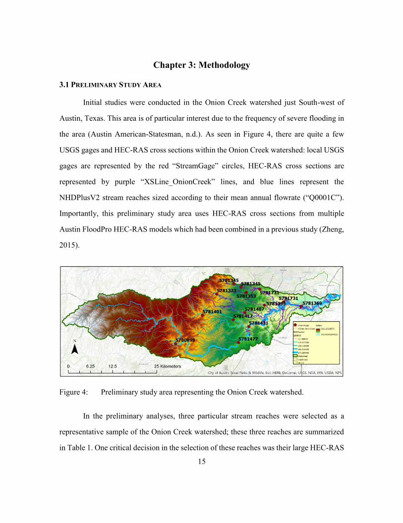
Initial studies were conducted in the Onion Creek watershed just South-west of

Austin, Texas. This area is of particular interest due to the frequency of severe flooding in

the area (Austin American-Statesman, n.d.). As seen in Figure 4, there are quite a few

USGS gages and HEC-RAS cross sections within the Onion Creek watershed: local USGS

gages are represented by the red “StreamGage” circles, HEC-RAS cross sections are

represented by purple “XSLine_OnionCreek” lines, and blue lines represent the

NHDPlusV2 stream reaches sized according to their mean annual flowrate (“Q0001C”).

Importantly, this preliminary study area uses HEC-RAS cross sections from multiple

Austin FloodPro HEC-RAS models which had been combined in a previous study (Zheng,

2015).

Figure 4: Preliminary study area representing the Onion Creek watershed.

In the preliminary analyses, three particular stream reaches were selected as a

representative sample of the Onion Creek watershed; these three reaches are summarized

in Table 1. One critical decision in the selection of these reaches was their large HEC-RAS

16

cross section density, enabling a more thorough analysis of HAND rating curves as

compared to HEC-RAS data. These stream reaches also needed to approximately represent

the range of variations present in the dataset, resulting in the selection of reaches of varying

lengths, USGS stream gage locations, and topographical ranges.

COMID Stream Reach

Length (ft)

USGS Stream

Gage Location

# HEC-RAS

Cross-

sections

Topography

Range (ft)

5781369 15,521 Downstream end 63 62.538

5781373 25,803 Upstream end 102 127.212

5781407 32,175 Middle 105 100.718

Table 1: Summary of three selected stream reaches for preliminary analysis.

As an aid to generally understand these reaches prior to analyzing them,

cartographic details for all of these reaches were generated in the form of 2-dimensional

and 3-dimensional maps (see Figures 5, 6, and 7). These maps helped inform where the

USGS gages were located along each stream reach as well as what the topography ranges

were for each stream reach.


COMID 5781369.

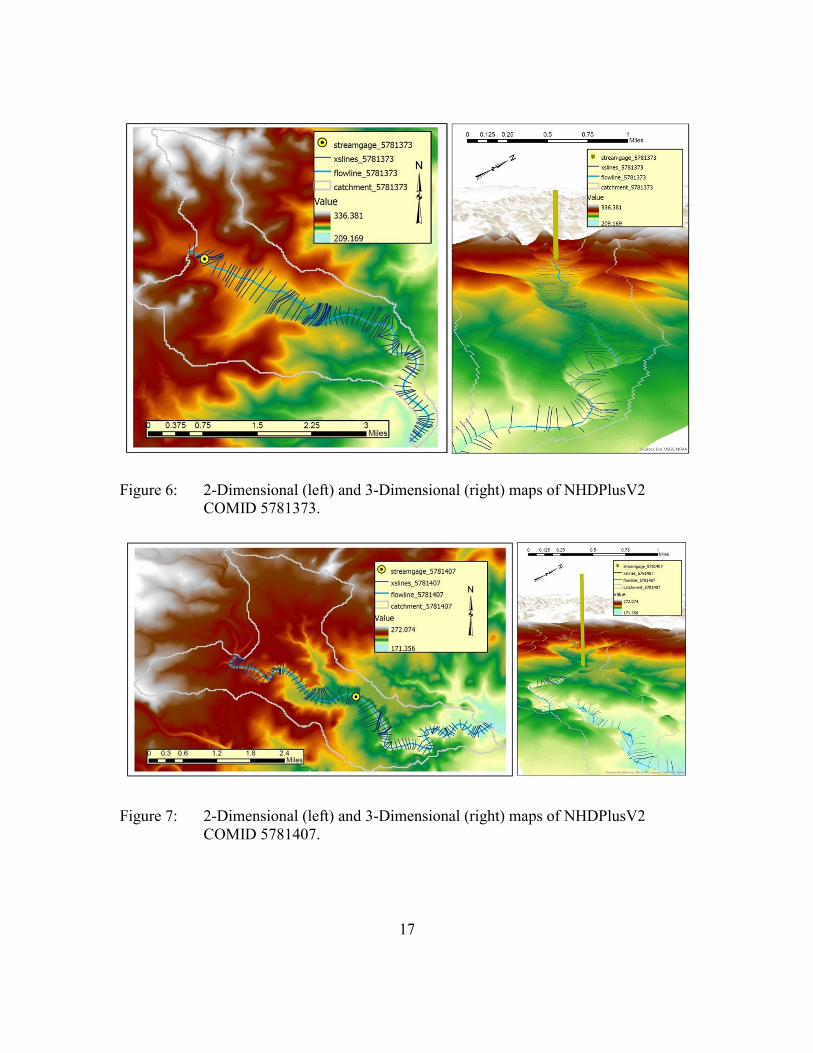
17


COMID 5781373.


COMID 5781407.

18

3.2 AVAILABLE DATA

This research relies primarily on two types of data along stream reaches: rating

curves and transverse cross sections. Transverse cross sections were collected for HAND

and USGS stream reaches primarily for preliminary analysis, after which the focus of this

research turned strictly to rating curves. HEC-RAS cross-sections were also collected

strictly with the purpose of converting them into HEC-RAS rating curves. Rating curve

data was also gathered for HAND and USGS stream reaches.

3.2.1 National Hydrography Dataset Plus Version 2

The National Hydrography Dataset Plus Version 2 (NHDPlusV2) approximately

represents all stream reaches throughout the CONUS (Mckay et al., 2012). In addition to

geographical locations for all stream reaches, each of these 2.67 million stream reaches has

additional data associated with it. Specifically relevant to this project, each NHDPlusV2

stream reach has an associated mean discharge in cubic feet per second (“Q0001C”), a

length in kilometers (“LengthKM”), and a unitless slope (“SLOPE”). Importantly, these

slopes are computed using NED elevations at each end of the reach in conjunction with the

length in kilometers of the stream reach (Mckay et al., 2012).

In addition to providing extensive data for each stream reach in the nation, the

NHDPlusV2 dataset organizes all stream reaches by hydrologic accounting regions called

Hydrologic Unit Codes (HUCs), which are for convenient organization and indexing.

These HUCs are widely used in hydrology for organization by different catchments, and

this same organization approach is used for the indexing of both the NWM discharge

outputs and the HAND database. Consequently, these HUCs were used throughout this

analysis in order to enable the use of available NHDPlusV2, NWM, and HAND data. In

addition, NHDPlusV2 stream reaches have unique “common identifiers” termed

19

“COMIDs”; COMIDs will be mentioned throughout this work to refer to specific stream

reaches in the NHDPlusV2 dataset.

3.2.2 HAND Data

Owing to extensive research, HAND hydraulic properties have been computed for

all NHDPlusV2 stream reaches in the CONUS (see Figure 8) (Liu et al., 2017). This

research was initially conducted through the National Flood Interoperability Experiment

(NFIE), hence the web portal’s url location: http://nfie.roger.ncsa.illinois.edu/nfiedata/.

These hydraulic properties are organized by 6-digit HUC (HUC-6) regions for convenient

organization and ease of use (Seaber, Kapinos, & Knapp, 1987). For all of these regions,

in addition to providing a myriad of hydraulic parameters, various datasets are also

available, such as DEM raster datasets and shapefiles.

20

Figure 8: National Flood Interoperability Experiment HAND Data Portal for HUC 6

“120902” (http://nfie.roger.ncsa.illinois.edu/nfiedata/HUC6/120902/).

For this investigation, these HAND rating curve parameters were programmatically

retrieved from .csv files containing all HAND data for specific HUC 6 watersheds. As seen

in Figure 8, these .csv files were named by HUC-6 code: “hydroprop-fulltable-<HUC6

stream reach identifier>.csv” (ie. hydroprop-fulltable-120902.csv for HUC 120902). Once

retrieved, this dataset provides all the information necessary for generating HAND rating

21

curves for all NHDPlusV2 stream reaches in the CONUS (with an assumed Manning’s

roughness of 0.05).

3.2.3 USGS Data

The USGS publishes an array of hydrologic data collected at their stream gages

scattered throughout the country (USGS, n.d.). One particular dataset contains information

for rating curves organized by online web address, as shown in Figure 9. These datasets

specifically provide streamflow (“INDEP”), stage height (“DEP”), and depth-shift

correction (“SHIFT”) information. These values are retrieved from frequent field

measurements of river cross sections at stream gage locations, coupled with automated

surface water depth measurements retrieved by these stream gages.

Figure 9: Representative sample of USGS Water Watch rating curve data for USGS

gage 08159000 representing Onion Creek at Highway 183

(https://waterdata.usgs.gov/nwisweb/get_ratings?file_type=exsa&site_no=0

8159000).

Cross section data are also available through another USGS Water Watch portal

containing more detailed information (see Figure 10). Specifically relating to cross

sections, this portal provides channel widths (“chan_width”), stage heights

22

(“gage_height_va”), and a data classifier (“current_rating_nu”). From this data,

symmetrical cross sections can be approximated that describe the most current USGS field

measurements.

Figure 10: Representative sample of USGS Water Watch detailed data for USGS gage

08159000 representing Onion Creek at Highway 183

(https://waterdata.usgs.gov/tx/nwis/measurements?site_no=08159000&agen

cy_cd=USGS&format=rdb_expanded)

Importantly, these USGS cross-sections do not include a Gage height at Zero Flow

(GZF) value; GZF values were instead shared by Kisters (a large data management firm

collaborating with much of the currently ongoing HAND research). Regrettably, GZF

values exist only for some USGS gages. Notably, the GZF value is of particular importance

because, similar to the bottom-depth shift implemented for all USGS rating curves, a GZF

represents the “actual” bottom of a river channel cross-section, rather than the measured

bottom on the day the stream was visited. A sample of the GZF values available for Onion

Creek are shown in Figure 11 below, showing both the organization of the table as well as

the fact that each steam gage may have multiple GZF shifts for each data point.

23

Figure 11: Gage height at Zero Flow (GZF) data available for three example stream

gages in the Onion Creek watershed. Data received from Kisters.

One final point is important: though using USGS rating curves is a seemingly

obvious approach for completing the discharge-to-stage-height conversion, the shortage of

USGS rating curve data as compared to the ~2.67 million stream reaches where the NWM

is now forecasting discharges is fairly substantial. This extreme shortage of rating curve

data must be resolved before this conversion can be reasonably implemented at the national

scale. Various approaches to resolving this problem have been undertaken, frequently

focusing on model simulations, at-a-station hydraulic geometries, remotely sensed data,

etc., though it is unclear if they will integrate appropriately with the new NWM forecasts

(Dingman, 2007; Smith & Pavelsky, 2008; Raymond, 2012). This work attempts to address

this concern by exploring alternatives to the USGS dataset, hopefully enabling future

national-scale rating curve approximations at all 2.67 million stream reaches.

3.2.4 HEC-RAS Data

HEC-RAS cross sections along with their associated Manning’s roughness values are

available from the Austin FloodPro Onion Creek HEC-RAS model (Figure 12) (City of

Austin, n.d.). In this visualization, the blue line represents the Onion Creek flowlines, while

green lines represents the HEC-RAS cross sections along the stream reaches. Within this

HEC-RAS model, all cross sections along the reach are uniquely identified by their so-

24

called River Station, named in accordance with their distance downstream. Further points

laying along the cross section are termed Stations, describing various distances along the

cross section with their associated elevation.

Figure 12: Austin FloodPro HEC-RAS Model for Onion Creek viewed in the HEC-

RAS 5.0.3 Desktop Application (City of Austin, n.d.).

An example cross section at River Station 55510 is shown in Figure 13,

corresponding to the cross section that is 55,510 feet downstream from the end of this HEC-

RAS model stream reach (ie. 0 marks the most downstream end of the reach). This cross

section corresponds to the precise location of the USGS stream gage representing Onion

Creek at highway 183 in Austin, Texas.

The cross section is represented by the black line, while the black dots along this

line represent individual Stations along this cross section. The two red dots denote the

divide between the main channel and the over bank channel. Further, the blue “WS” lines

and green “EG” lines represent the water surface lines and energy grade lines, respectively.

25

The black “Ground” line seems to have been added as a representation of bridge piers (to

restrict water from entering these areas), which would be consistent with the bridge upon

which this gage is placed.

Figure 13: River Station 55510 from Austin FloodPro HEC-RAS Model for Onion

Creek viewed in the HEC-RAS 5.0.3 Desktop Application (City of Austin,

n.d.).

3.3 PRELIMINARY RATING CURVE ASSESSMENTS

Throughout the preliminary study area, HAND, USGS, and HEC-RAS rating

curves were constructed for all stream reaches. This rating curve creation is described in

the following sections.

26

3.3.1 HAND Rating Curves

HAND rating curves were constructed using Manning’s equation. First, S0 was

retrieved from the NHDPlusV2 dataset (Mckay et al., 2012). The HAND methodology was

then used to determine Aw and HR for all stream reaches at specified depth intervals (ie.

every 1 foot). Rather than re-compute these hydraulic properties, this data was retrieved

through the NFIE portal (NFIE, n.d.). Given these hydraulic properties, the only remaining

variable required was Manning’s roughness coefficient, n.

Manning’s roughness can either be retrieved from existing data sources (such as

USGS field measurements or HEC-RAS models), or can be determined in the field through

observations. Seeing as Manning’s roughness values are not currently available for all 2.67

million NHDPlusV2 stream reaches, a Manning’s roughness of n = 0.05 was initially

assumed. This value was selected simply because it is an average Manning’s roughness

value, describing a natural stream that is “winding with weeds and pools” (Chow,

Maidment, & Mays, 1988). Finally, using all these data, Manning’s equation was used to

compute discharge for all depth intervals, enabling the generation of synthetic HAND

rating curves such as that shown in Figure 14.

27

Figure 14: Preliminary HAND rating curve for Onion Creek stream reach COMID

5781369.

By stacking HAND top widths at varying stage heights on top of each other, HAND

cross sections can also be created using the HAND methodology (see Figure 15). The two

sides of each HAND cross section (centered on the bottom point) are then reflectively

symmetric to one another. While this is not precisely representative of a physical channel,

this assumption was necessary for this approach to work appropriately. It is important to

note that HAND rating curves are unrelated to this methodology and are therefore

uncompromised. Additionally, this HAND cross section has not been shifted to correct its

geodetic datum; this correction was identified and explored in further sections of the work.

28

Figure 15: Preliminary HAND cross section for Onion Creek stream reach COMID

5781369.

3.3.2 USGS Rating Curves

USGS rating curve data was retrieved by programmatically scraping the USGS

online Water Watch database with customized Python scripts. These scripts were written

to retrieve stage height, discharge, and depth-shift data before plotting rating curves for

visual analysis (see Figure 16). The depth-shift data describes a stage height correction

based on USGS field measurements. This depth-shift correction was consequently applied

to all USGS rating curves henceforth presented in this research work.

29

Figure 16: Preliminary USGS rating curve for Onion Creek stream reach COMID

5781369 (USGS gage 08159000).

Identical to the construction of HAND rating curves, USGS channel width data

were also available. Channel width information was collected and stacked on top of itself

according to the related stage heights, creating another form of reflectively symmetrical

cross section (see Figure 17). Importantly, the dataset containing channel width

information also included a classifier grouping the data into groups. The USGS changes

these groupings whenever a stream reach’s hydraulic properties vary significantly,

meaning that only the most recent group could be meaningfully compared to the HAND

30

cross sections. As such, this classifier was used as a selection tool to collect cross section

data only for the most recent and up-to-date channel widths available. While this

significantly shrinks the dataset, this isolation of only the more recent data was necessary

to maintain cross section continuity without including erratic outliers. Notably, this USGS

cross section has not been shifted to account for its geodetic datum; this correction was

identified and explored in further sections of the work.

Figure 17: Preliminary USGS cross section for Onion Creek stream reach COMID

5781369 (USGS gage 08159000).

31

3.3.3 HEC-RAS Rating Curves

In the preliminary analysis of HEC-RAS rating curves, information from a previous

study compiling Austin FloodPro data and generating rating curves for Onion Creek was

used (Zheng, 2015). In this study, HEC-RAS rating curves were created by exporting the

available Hydrologic Engineering Center Data Storage System (HEC-DSS) rating curve

file, making this data accessible outside of the HEC-RAS model. This process involves

reading the HEC-DSS file using a DSS Utility Program (DSSUTL), retrieving the

minimum channel elevation of each HEC-RAS cross-section using the HEC-RAS API –

HEC-RASController (for VBA integration), locating each cross-section’s rating curve

using the HEC-RAS River Station nomenclature (detailing the length downstream of each

cross-section), and wrapping all this data up together (Zheng, 2015). From this study, a

.csv file summarizing HEC-RAS rating curve data for the Onion Creek watershed was

available in .csv format (Zheng, 2015).

These HEC-RAS rating curves were then collected and plotted with a Python script

(see Figure 18). As in the figure, most NHDPlusV2 catchments have multiple HEC-RAS

cross sections within them, resulting in the generation of various HEC-RAS rating curves

for each stream reach. Notably, these rating curves are comprised of five hypothetical flood

discharges, each representing a point along the rating curve: the 10-year, 25-year, 50-year,

100-year, and 500-year floods. These flood discharges were then plotted as linearly-

interpolated lines, consequently resulting in the sharp angle at the front end of the curve

(between the origin and the 10-year hypothetical flood discharge).

32

Figure 18: Preliminary HEC-RAS rating curves for Onion Creek stream reach COMID

5781369.

An additional output from this analysis is a shapefile representation of all HEC-

RAS cross sections. This output can be viewed and analyzed in ArcGIS or other spatial

analysis software, as was shown in Figures 10 through 13.

3.3.3.1 Power-Law Curve Fitting

Many of the rating curves derived in this work rely on only a few points which must

be generalized with a curve fitting. For this curve fitting, a power-law fit was used due to

its acceptance in rating curve literature (Reistad, Petersen-Øverleir, & Bogetveit, 2005;

Dingman, 2007). Notably, because a power-law function thins out exponentially, marginal

https://www.researchgate.net/profile/Asgeir_Petersen-Overleir

33

changes in rating curve stage heights eventually become associated with enormous changes

in discharge, creating significant under-approximations of stage height moving forward.

Despite this complication, a power-law fit generally looks significantly better than a linear

regression, and consequently this fitting was used throughout this work. Particularly at

lower stage height values, a power-law fit greatly improves the curvature of a rating curve,

again justifying its use.

The power-law relationship used in this work is defined by the following equation,

where A and B are constants describing the particular rating curve which is being fit:

𝑦 = 𝐴𝑥𝐵

Power-law curve fitting was accomplished first through a programmatic

transformation of all HEC-RAS curves to a natural log – natural log relationship. Following

this transformation, a linear fitting of the data was possible, and this fit enabled a

computation of the slope (B) and the intercept (logA) of each line. With a bit more

manipulation, each HEC-RAS line was successfully fitted with a power-law line, enabling

queries on the HEC-RAS dataset at all stage heights.

3.3.3.2 Resistance Function

In an effort to better understand the large spread of cross-sectional rating curve

variation, multiple box-plots were plotted for every stage-height for all reaches in the study

area containing HEC-RAS cross-section data. An example of this visual analysis is shown

in Figure 19.

34

Figure 19: Boxplots denoting the spread of HEC-RAS rating curves for stream reach

COMID 5781369.

Following this comparison, HEC-RAS rating curves comparable to the HAND and

USGS rating curves were generated using a reach-averaged representation of all HEC-RAS

rating curves. This relationship was derived as a “resistance function”, so named due to its

dependency on variable Manning’s roughness coefficients. Importantly, this is not

constructed through an averaging of rating curve values at varying stage heights, instead it

depends on back-calculated Manning’s roughness values at every stage height.

To construct the resistance functions for each catchment, a Manning’s roughness

value was back-calculated for each stage height between 0 and 82 feet (this extent of stage

35

heights was chosen for consistency with the HAND rating curve stage height data). This

back-calculation relied on NHDPlusV2 slope values as well as HAND wetted area and

hydraulic radius values. Using this information and the discharge (retrieved by reading

each HEC-RAS rating curve for the stage height in question), a Manning’s roughness was

computed for each HEC-RAS curve at that particular stage height. Once all of these

Manning’s roughness values were computed, all these roughness values within a stream

reach could be averaged together by stage-height (ie. one roughness average for every 1-

foot stage height interval), and a single representative rating curve, the “resistance

function”, could be created describing the entire reach (see Figure 20).

36

Figure 20: Preliminary HEC-RAS rating curves for Onion Creek stream reach COMID

5781369 (in grey) with “resistance function” (in red).

3.4 PRELIMINARY CROSS SECTION ASSESSMENTS

In addition to rating curve analyses, cross sections were also explored as a

potentially useful metric for assessing the performance of the HAND methodology. This

comparison was only conducted between HAND and USGS cross sections in avoidance of

the monstrous variations of the HEC-RAS cross sections.

3.4.1 HAND Cross Sections

HAND cross sections were created using the channel width and stage height data

available through the NFIE web portal. A Python script was written to iterate through all

37

stage heights and channel widths, consequently stacking them up on top of each other in a

typical cross sectional plot. These cross sections were then positioned at the appropriate

elevation using geodetic datum elevations retrieved using ArcGIS.

Seeing as a HAND cross-section is representative of a whole reach, the geodetic

datum was collected at the USGS gage location from the 10-meter NED upon which

HAND is generated. This was done for consistency when comparing with the USGS

location which (ideally) would have a similar geodetic datum value. In order to collect this

geodetic datum value, the USGS gages first had to be snapped to their nearest NHDPlusV2

streamline using the ArcGIS “snap” tool. Following this spatial adjustment, the 10-meter

NED was read at each USGS gage in question using the ArcGIS “Extract Multi Values to

Points” tool, resulting in a table containing COMIDs and 10-meter NED elevations. These

elevations were treated as the representative geodetic datum of the HAND cross sections,

depending on the COMID of the HAND stream reach. An example HAND cross section

constructed in this way is shown in Figure 15.

3.4.2 USGS Cross Sections

Constructed similarly to the HAND cross sections, USGS cross sections relied on

width and depth data, with an additional depth shift step required. This depth shift was

collected from the GZF values corresponding to these USGS stream gages, though notably

only the most recent GZF value was used for each stream gage, rather than an average of

all previously observed GZF values together. Additionally, not all USGS stream gages in

the Onion Creek watershed contained GZF adjustments, thereby nullifying the relevance

of any HAND and USGS cross section comparisons for these stream reaches.

Once USGS cross sections were collected and properly tweaked according to any

GZF data available, the geodetic datum describing the elevation above sea level was

38

retrieved for each cross-section. The geodetic datum information for all USGS gaging

stations is available on each cross-section’s Water Watch webpage (USGS, n.d.); this data

was scraped from the web for all COMIDs in question using another Python script.

Specifically for the USGS gages, a particular spatial reference of the datum was

retrieved as well, as some gages were listed using the National Geodetic Vertical Datum

of 1929 (NGVD 29) while others used the North American Vertical Datum of 1988

(NAVD 88). Importantly, these two reference systems are similar but different, meaning

that in a more complex study a conversion may be necessary to precisely retrieve USGS

elevations. In this fundamental assessment this conversion was ignored, seeing as the

conversion would likely create errors of up to only a few feet (FEMA, 2013). This was

acceptable for the visual comparisons made in this work. An example USGS cross section

constructed using this methodology is shown in Figure 17.

3.5 REVISED STUDY AREA

Over the course of this study, it became apparent that analysis at the river level

would be more informative than at the watershed level. After realizing this, the study area

was adjusted to reflect a new focus on Onion Creek as a river rather than the entire

watershed. As shown in Figure 21, local USGS gages are represented by the red

“OnionCk_StreamGages” circles, HEC-RAS cross sections are represented by purple

“OnionCk_XSects” lines, and NHDPlusV2 stream reaches are represented by blue lines

sized according to their mean annual flowrate (“Q0001C”). This change was made

primarily for two reasons. First-off, the initial reasoning for studying Onion Creek as a

sample set of various catchments throughout the Onion Creek area was due to the

availability of USGS data; this USGS data was later determined to be less useful than the

HEC-RAS data for this analysis, so this benefit was no longer relevant. The second reason

39

is that observation across a continuous stream reach enabled more thorough analysis not

only of roughness values and slopes (which both affect rating curves), but also of the way

these parameters change along the stream reach as one larger entity. These analyses were

considered to be critical for the overall generalization of the HAND methodology on a

larger scale, and therefore this shift in study area was necessary.

Figure 21: Revised study area representing only Onion Creek rather than the entire

Onion Creek watershed.

As shown in Figure 21, HEC-RAS cross section data are available for the entirety

of Onion Creek, while USGS gaging stations are only available at three locations (one of

which contains no useful HEC-RAS data for comparison, so truly data for only two USGS

40

gages is useful). Due to this relative scarcity of USGS data, comparison between HAND

and HEC-RAS rating curves became the focus of analysis moving forward.

3.6 STREAM PROFILE

Once the study area was revised, the next step in comparing HAND and HEC-RAS

data was to recognize that HAND is generated using the NED DEM. As such, any

differences between the NED and the elevations used in the Onion Creek HEC-RAS model

would be informative. Consequently, the next study involved a stream profile comparison

between the HAND and HEC-RAS stream profiles. USGS data was not included due to

the relative scarcity of information along Onion Creek; any attempt to create a stream

profile would have had only two or three points along Onion Creek, resulting in an

uninformative stream profile.

For this comparison, only the minimum elevation value is needed from the HEC-

RAS dataset, and thus all other cross-section Stations were removed. The results of this

generalization were arrived at by relating each RiverStation only to its lowest Station’s

elevation value (see Figure 22, where “RAS” is the column denoting the HEC-RAS lowest

elevation values).

41

Figure 22: Sample of River Stations for cross sections along Onion Creek with their

associated minimum HEC-RAS elevations.

After simplifying the HEC-RAS data, minimum DEM elevations were retrieved for

each HAND stream reach using a raw DEM (“120902.tif”), a filled DEM (“120902.fel”),

and DEM-derived flowlines (“120902.src”) (NFIE, n.d.). All these data were specified by

HUC-6, similar to all other HAND data organization seen previously in Figure 8. The raw

DEM is simply a normal DEM, the filled DEM has all pits removed, and the DEM-derived

flowlines are the equivalent of the NHDPlusV2 flowlines except that they are derived from

the DEM (and consequently differ slightly). Before processing, only the DEM-derived

flowlines intersecting the Onion Creek cross sections were selected and exported to a new

shapefile.

Using these datasets along with a shapefile of the HEC-RAS cross sections, a

customized ArcGIS script was used to extract the values of the filled and unfilled DEMs

where each HEC-RAS cross section intersects with the DEM-derived flowlines. The results

42

of this data extraction are shown in Figure 23, displaying each River Station along with its

DEM and FEL (filled DEM) values (in feet).

Figure 23: Sample of River Stations and associated unfilled (DEM) and filled (FEL)

DEM values extracted from the NED.

These values were then combined with the HEC-RAS minimum elevations (Figure

22) and plotted as a stream profile for comparison. The result of this comparison for Onion

Creek is shown in Figure 24, displaying the minimum elevation differences between

HAND (represented by DEM and FEL) and the HEC-RAS model. The DEM-based stream

profiles vary significantly more than the HEC-RAS stream profile, resulting in more slope

variability throughout the stream reach. This has problematic implications on slope which

will be explored later.

43

Figure 24: Stream profile showing HAND (DEM and FEL) and HEC-RAS (RAS)

elevations along the entire length of Onion Creek.

3.7 DETAILED RATING CURVE ASSESSMENTS

As this research progressed, the focus shifted from locating individual HEC-RAS

cross-sections for each stream reach to become a more thorough analysis using reach-

averaged median HEC-RAS rating curves (this is different from the above-described

resistance function curves). These reach-averaged HEC-RAS rating curves were then

methodically compared to HAND rating curves to resolve any differences. Additionally,

the study area revisions enable the entirety of Onion Creek to be assessed, searching for

generalizable trends in HEC-RAS rating curve differences as compared to HAND rating

curves. These generalizable differences are the real question, with the true objective being

the elimination of HAND inconsistencies on a national scale.

44

3.7.1 Revised HEC-RAS Rating Curves

Using a Python script, Onion Creek cross section data was extracted from the HEC-

RAS model. The results of this extraction are a .csv output summarizing the data at all

points on the HEC-RAS cross section, specifically capturing each point’s Station and

Elevation as shown in Figure 25. The Station value describes how far along the cross

section each point is (in feet, following the cross section’s length), and the Elevation is

simply the elevation of each of these Stations (also in feet).

Figure 25: Sample of Onion Creek HEC-RAS cross section data extracted from the

model and summarized in .csv format.

Using this information, HEC-RAS rating curves for various discharge values were

created for all HEC-RAS cross sections. To generate these rating curves, various discharge

values were first collected for each stream reach before they could be run through the HEC-

RAS model. From the NHDPlusV2 dataset, mean annual discharge was collected for all

locations where HEC-RAS River Stations and NHDPlusV2 flowlines intersect. A sample

of this data after it was extracted is shown in Figure 26, representing each river station and

the mean annual flow for the NHDPlusV2 stream reach it intersects (denoted by the

“Q0001C” column).

45

Figure 26: Sample of Onion Creek HEC-RAS River Stations and associated

NHDPlusV2 mean annual discharge (“Q0001C”).

These mean annual flow data were then simplified by removing any duplicated

COMIDs. This was done by selecting only the most upstream River Station in each

COMID, and removing all other River Stations that share the same COMID value.

Logically this is acceptable because the NHDPlusV2 mean annual discharge values are

unique only at the stream reach scale, meaning that, as seen in Figure 26 above, these mean

annual discharges are identical for all River Stations with the same COMID. This removal

of downstream River Stations therefore did not impact the HEC-RAS model results.

3.7.1.1 USGS 100-year Flood Regression

Following the collection of this data, a 100-year flood regression was computed

using a flood regression methodology derived by the USGS (Asquith & Roussel, 2009).

This flood regression methodology is based on the following equation:

𝑄100 = 𝑃1.071𝑆0.50710[0.969Ω+10.82−8.448𝐴−0.0467]

46

Where Q100 represents the 100-year discharge, P represents mean annual

precipitation (inches), S is the main-channel slope, Ω is a generalized terrain and climate

index, and A represents the drainage area (square miles).

Using this equation, a 100-year flood discharge was computed for all catchments

along Onion Creek. Annual precipitation draining to each stream reach, channel slope of

each stream reach, and drainage area to each stream reach were all retrieved from the

NHDPlusV2 dataset as “P_inch”, “SLOPE”, and “TotDASqMI”, respectively. The

OMEGA value was retrieved from Figure 26, retrieved from the USGS work in which the

equation was derived (Asquith & Roussel, 2009). According to Figure 27, the OMEGA

value for all of Onion Creek is 0.125. Figure 28 shows an example of this calculated 100-

year flood discharge for COMID 5781939 using the stream reach’s local NHDPlusV2

properties and the Onion Creek OMEGA value of 0.125.

47

Figure 27: Omega parameter representing a generalized terrain and climate index for

Texas (Asquith & Roussel, 2009).

Figure 28: Example of calculated 100-year flood discharge for COMID 5781939.

48

3.7.1.2 Slope Assumption

Before continuing with the analysis, the flood regression 100-year flood discharge

was compared to the HEC-RAS 100-year flood discharge (retrievable from the HEC-RAS

model) for each stream reach. In the case of Onion Creek, these values differed

significantly, and as such the slope was modified to approach a more reasonable 100-year

discharge. Initially this shift was made by using a calculated average slope of all Texas

stream reaches (0.00623), but this slope still resulted in a significant error and was therefore

not as useful as anticipated.

Finally, the optimal slope for creating a minimal difference between the HEC-RAS

and HAND 100-year floods curves was computed for Onion Creek as 0.00999, and the

flood-regression slope was manually changed to this value. After this change, both 100-

year flood values matched much better, and the analysis could continue. It is very important

to note that this was initially considered an unreasonable approach. However, after careful

assessment, it was ultimately determined that the intent of this research is to improve the

relationship between discharge and stage height (ie. rating curves), and as such determining

the correct discharge was not within this scope. This is particularly true seeing as

discharges from the NWM will ultimately be used for any real-time flood forecasting.

Consequently, this manipulated discharge value was used to match HEC-RAS 100-year

flood discharges as closely as possible while still remaining consistent in its derivation

method using the USGS equation introduced above.

3.7.1.3 Final HEC-RAS Rating Curves

After correcting these discharge assumptions, a series of eight linearly-interpolated

discharge values were generated between the mean annual flow (“Q0001C” from

NHDPlusV2) and the 100-year flood discharge (100-year flood regression discharge using

a manually corrected slope). Eight values were selected as a good balance to maintain

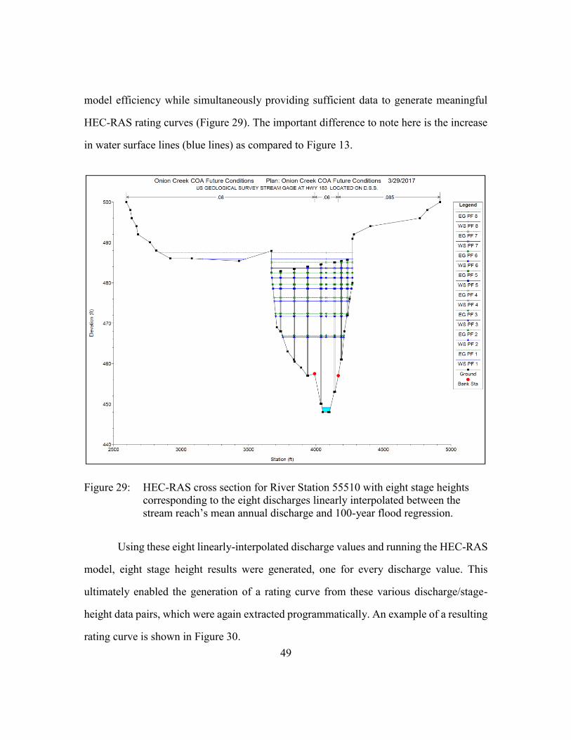
49

model efficiency while simultaneously providing sufficient data to generate meaningful

HEC-RAS rating curves (Figure 29). The important difference to note here is the increase

in water surface lines (blue lines) as compared to Figure 13.

Figure 29: HEC-RAS cross section for River Station 55510 with eight stage heights

corresponding to the eight discharges linearly interpolated between the

stream reach’s mean annual discharge and 100-year flood regression.

Using these eight linearly-interpolated discharge values and running the HEC-RAS

model, eight stage height results were generated, one for every discharge value. This

ultimately enabled the generation of a rating curve from these various discharge/stage-

height data pairs, which were again extracted programmatically. An example of a resulting

rating curve is shown in Figure 30.

50

Figure 30: HEC-RAS median rating curve for COMID 5781369, with box plots

representing the spread of all HEC-RAS curves within this COMID.

3.7.2 HAND vs. HEC-RAS

Using the current HAND assumption of Manning’s roughness equal to 0.05, a

preliminary look at the differences of HAND and HEC-RAS can be observed. An initial

look at this (see Figure 30) shows that, though there are differences between the blue

HAND curve and the red HEC-RAS curve, the 0.05 assumption seems to perform quite

well for this particular stream reach. This form of visual comparison will be revisited in

the results section, exploring alternative HAND rating curves and their performance.

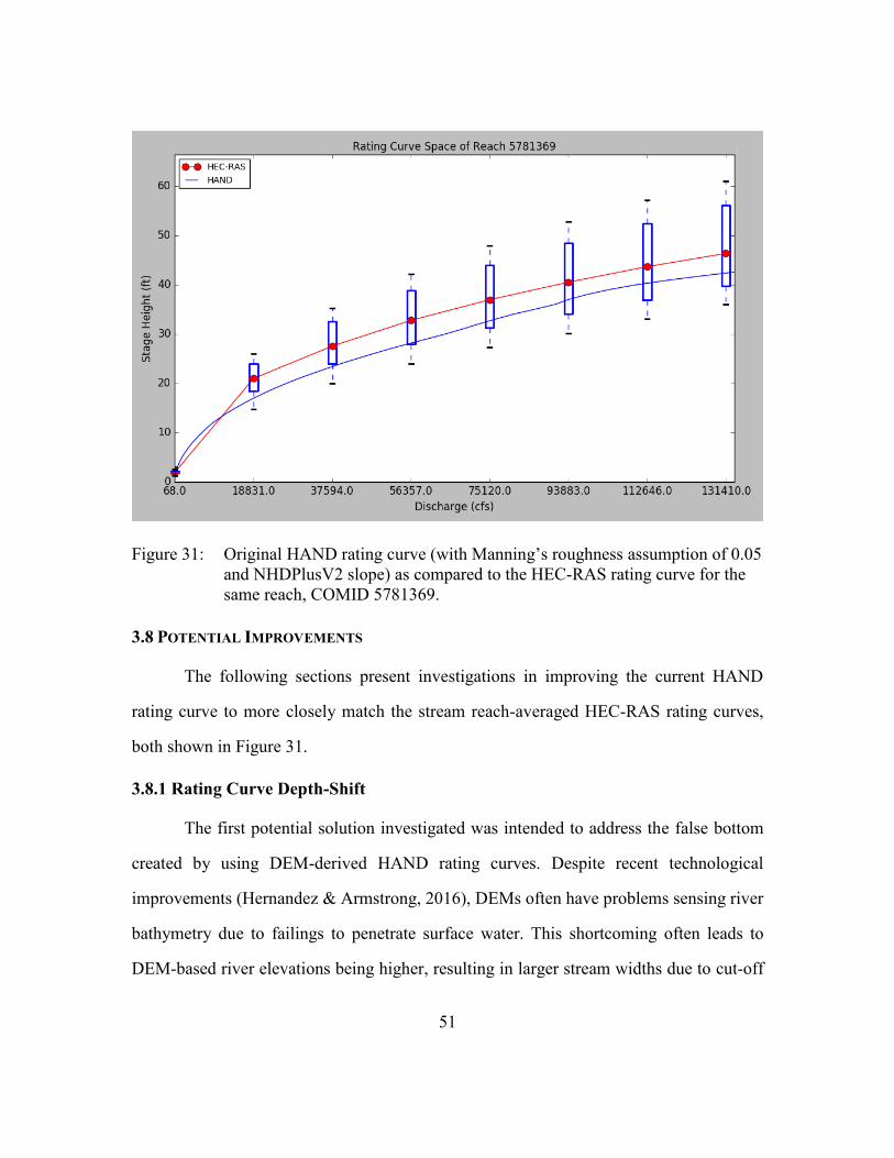
51

Figure 31: Original HAND rating curve (with Manning’s roughness assumption of 0.05

and NHDPlusV2 slope) as compared to the HEC-RAS rating curve for the

same reach, COMID 5781369.

3.8 POTENTIAL IMPROVEMENTS

The following sections present investigations in improving the current HAND

rating curve to more closely match the stream reach-averaged HEC-RAS rating curves,

both shown in Figure 31.

3.8.1 Rating Curve Depth-Shift

The first potential solution investigated was intended to address the false bottom

created by using DEM-derived HAND rating curves. Despite recent technological

improvements (Hernandez & Armstrong, 2016), DEMs often have problems sensing river

bathymetry due to failings to penetrate surface water. This shortcoming often leads to

DEM-based river elevations being higher, resulting in larger stream widths due to cut-off

52

channel bottoms, and ultimately decreasing stage heights. This could easily be a reason for

the HAND curve being lower than the HEC-RAS curve in Figure 30.

In resolving this issue, the HEC-RAS cross-sections were used as a guide by

retrieving the HEC-RAS depth at zero discharge. This depth was determined by finding

the width of the river reach at a HAND depth of zero feet (width is determined by summing

the number of pixels along the transverse axis to the reach). A corresponding discharge is

then read off of the median HEC-RAS rating curve, resulting in a discharge shift. Once

these values were determined, the HAND rating curve was adjusted to reflect the physical

depth captured by the HEC-RAS rating curve (which is assumedly missed by the HAND

rating curve). Similarly, a shift in discharge was also applied to account for the discharge

that would exist in this false bottom if it was accounted for. After this analysis, the HAND

rating curves were generally shifted up, beginning at a positive depth and discharge (rather

than at the origin), as shown in Figure 32.

53

Figure 32: HAND rating curve with a depth shift applied (with Manning’s roughness

assumption of 0.05 and NHDPlusV2 slope) as compared to the HEC-RAS

rating curve for the same reach, COMID 5781369.

3.8.2 Manning’s Roughness Edits

In an effort to further improve the fit of the HAND rating curves, edits to the 0.05

roughness assumption were explored next.

3.8.2.1 NLCD Catchment Averaged Roughness

Attempting to intelligently determine Manning’s roughness for all stream reaches

in the CONUS, roughness relationships between Manning’s roughness and the 2011

National Land Cover Database (NLCD) (Homer et al., 2015) were sought out. Luckily, an

informative review summarized and generalized previous findings to relate a Manning’s

roughness value to all NLCD classifications as follows (Figure 33) (Moore, 2011).

54

Figure 33: Manning’s roughness by National Land Cover Database classification

(Moore, 2011).

After retrieving NLCD data for Onion Creek (Homer, 2011), these new Manning’s

roughness values were re-mapped to the NLCD grid before being averaged for each Onion

Creek NHDPlusV2 catchment. Using these new catchment-averaged roughness values,

HAND discharges were re-computed using Manning’s equation, resulting in different

rating curve outputs. These outputs, with and without the depth-shift previously described,

are summarized in Figure 34 for COMID 5781369. As shown, all three edited options are

preferable to the currently available HAND rating curve (no depth-shift and a roughness

assumption of 0.05).

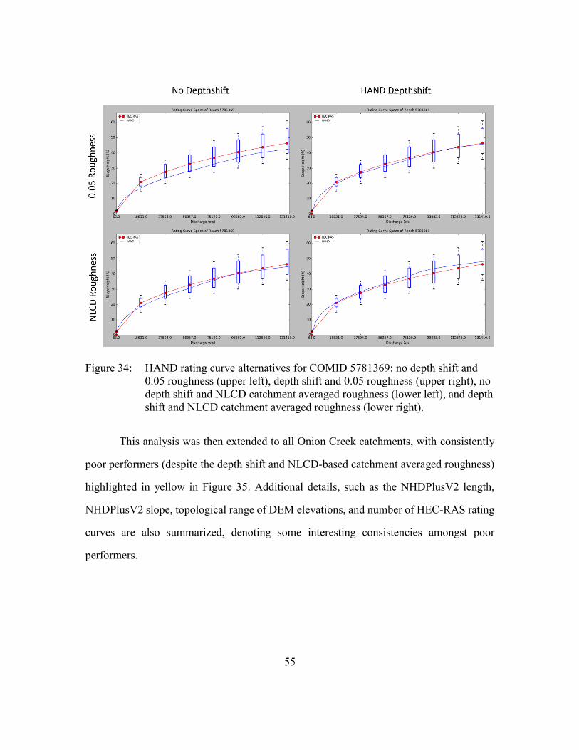
55

Figure 34: HAND rating curve alternatives for COMID 5781369: no depth shift and

0.05 roughness (upper left), depth shift and 0.05 roughness (upper right), no

depth shift and NLCD catchment averaged roughness (lower left), and depth

shift and NLCD catchment averaged roughness (lower right).

This analysis was then extended to all Onion Creek catchments, with consistently

poor performers (despite the depth shift and NLCD-based catchment averaged roughness)

highlighted in yellow in Figure 35. Additional details, such as the NHDPlusV2 length,

NHDPlusV2 slope, topological range of DEM elevations, and number of HEC-RAS rating

curves are also summarized, denoting some interesting consistencies amongst poor

performers.

56

Figure 35: Summary of all Onion Creek COMIDs, with consistently poor performers

highlighted in yellow.

From Figure 35, the poor performers appear to generally occur for shorter reaches

with smaller slopes. Notably, reaches with a smaller number of HEC-RAS cross sections

are less authoritative, due to the fact that HEC-RAS cross section rating curves are highly

dependent on their precise location along a reach. This means that reaches with fewer HEC-

RAS cross sections have a less precise median HEC-RAS rating curve with which the

respective HAND rating curve was compared. This naturally introduces error. NLCD

roughness values were then similarly compared for all stream reaches with no obvious

conclusions (see Figure 36).

Figure 36: Summary of land cover prevalence in all Onion Creek COMIDs. Column

headings correspond to specific NLCD classifications.

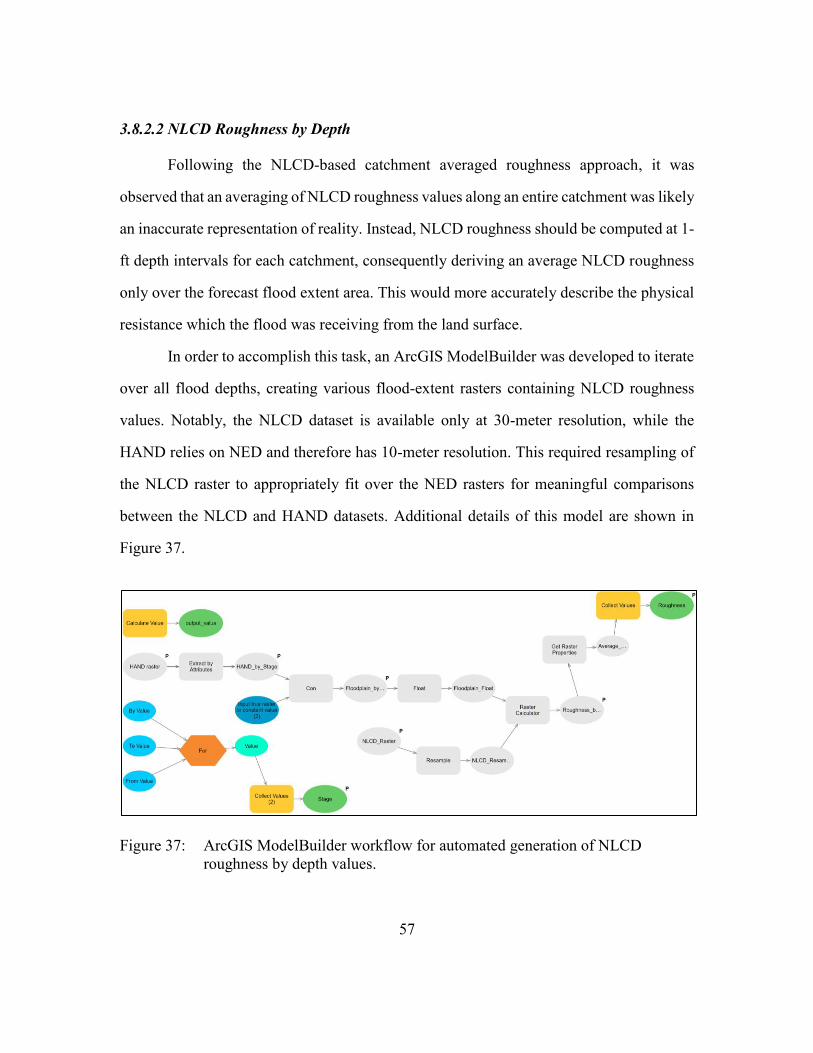
57

3.8.2.2 NLCD Roughness by Depth

Following the NLCD-based catchment averaged roughness approach, it was

observed that an averaging of NLCD roughness values along an entire catchment was likely

an inaccurate representation of reality. Instead, NLCD roughness should be computed at 1-

ft depth intervals for each catchment, consequently deriving an average NLCD roughness

only over the forecast flood extent area. This would more accurately describe the physical

resistance which the flood was receiving from the land surface.

In order to accomplish this task, an ArcGIS ModelBuilder was developed to iterate

over all flood depths, creating various flood-extent rasters containing NLCD roughness

values. Notably, the NLCD dataset is available only at 30-meter resolution, while the

HAND relies on NED and therefore has 10-meter resolution. This required resampling of

the NLCD raster to appropriately fit over the NED rasters for meaningful comparisons

between the NLCD and HAND datasets. Additional details of this model are shown in

Figure 37.

Figure 37: ArcGIS ModelBuilder workflow for automated generation of NLCD

roughness by depth values.

58

This ModelBuilder produced different NLCD-based roughness rasters for all Onion

Creak stream reaches at each different flood depth, from 0 through 82 feet (to maintain

consistency with available HAND flood depth data). Three example flood inundation

depths with their respective NLCD-based roughness rasters are shown in Figure 38 for

COMID 5781369.

Figure 38: NLCD roughness rasters for COMID 5781369 representing HAND flood

extents derived at inundation depths of 1 foot (left), 40 feet (center), and 80

feet (right).

After generating these models, a Python script was written to read through the

ModelBuilder log files, retrieving the average of all NLCD roughness values within the

NLCD roughness rasters. Using this methodology, averaged Manning’s roughness values

were computed for each COMID for all flood inundation depths between 0 and 82 feet,

resulting in NLCD depth-averaged roughness values, or NLCD roughness by depth. An

example rating curve generated using the previously described depth shift combined with

this new NLCD roughness by depth approach for computing Manning’s roughness is

shown in Figure 39. While most rating curves show an improvement using this approach,

this combination appears to worsen the result for this particular stream reach.

As is shown in Figure 34, the depth-shift (which has a sound theoretical basis)

seems to be an improvement both when using the assumed Manning’s roughness of 0.05,

and when using the NLCD averaged roughness (which for this reach is approximately

59

0.59). The NLCD roughness by depth for this reach varies by depth from about 0.086 at 0

feet down to 0.068 at 80 feet. According to the Onion Creek HEC-RAS model, the

roughness in this reach is generally 0.06, and very rarely at 0.055. Seeing as the Manning’s

roughness initially assumed is fairly close to the “correct” HEC-RAS roughness, as is the

NLCD average roughness, this reach happens to see better agreement in these two

instances. Conversely, in the case of the NLCD roughness by depth approach, the

Manning’s roughness values are too large initially (causing the curve to over-estimate the

computed discharges), and even on the tail end of the curve this roughness remains too

large.

Figure 39: HAND curve using the depth shift and NLCD roughness by depth

adjustments, COMID 5781369.

60

3.8.3 Slope Edits

Another problem identified in the initial rating curve analysis was the appearance

of overly-gradual slopes throughout Onion Creek. As seen in Figure 35, the poor

performers frequently had slopes around 0.00001, which is essentially a flat stream reach

with no elevation gradient. While this is theoretically possible, the results previously found

in the Onion Creek stream profile Figure 24) show that the DEM and FEL-derived stream

profiles vary significantly more than the HEC-RAS stream profiles. This decreasing overall

confidence in the NHDPlusV2 slopes due to their jaggedness.

3.8.3.1 DEM Slope

In attempting to correct for this, a more detailed slope analysis was conducted to

generate alternative slopes to those available through the NHDPlusV2. This was done by

averaging hydrologic slopes along DEM-derived channels for each catchment, where a

DEM-derived flowline is simply a 1-cell wide channel defining the lowest points of

drainage passing through a catchment. These DEM-derived channels are published on the

HAND webpage as a “.src” file for all HUC-6 regions (NFIE, n.d.). An additional dataset

collected from the HAND webpage was the “.slp” file containing slope data; this dataset

describes the hydrologic slope, or the steepest vertical slope, of each cell in the area (NFIE,

n.d.).

First, the data was cleaned by extracting only data within the catchments in

question. The hydrologic slope values were then conditionally selected solely where they

intersected with the DEM-derived flowline, ultimately returning slopes for every cell along

each catchment’s flowline. These slopes-along-each-flowline were averaged together for

each reach, resulting in an average DEM-derived slope over each stream reach, in theory

roughly equivalent to the NHDPlusV2 slopes (see Figure 40).

61

Figure 40: DEM-derived average flowline slopes for all Onion Creek catchments.

3.8.3.2 Slope Complications

Observing the results in Figure 40, there is clearly a problem with the very last

reach, COMID 5781939. The slope of this reach is zero, which – whether it makes physical

sense or not – will cause problems in the HAND model at this catchment, resulting in very

extremely inaccurate rating curves for flood prediction.

In attempting to understand the reason for this zero slope, a closer analysis of

COMID 5781939 was conducted. Plotted in Figure 41 is COMID 5781939 with a green

outline denoting the catchment, blue-and-orange lines denoting the DEM-derived flowline,

and the black-and-white background denoting hydrologic slope values across the entire

reach (black is zero slope, white is 100% slope). Blue cells along the flowline have a slope

of zero, while orange cells represent any positive, non-zero slope. From Figure 41 the

reason for a zero average slope of the reach becomes very clear: all hydrologic slope values

62

along the flowline for this catchment have a value of zero, thus resulting in an average

hydrologic slope of zero along the whole reach. Similarly, while there are slope values on

the two neighboring catchments, there are apparently a very large fraction of data points

with zero slope in these reaches as well. This is problematic and currently unresolved.

Figure 41: Hydrologic slope values in and around COMID 5781939.

3.8.3.3 Catchment-Averaged and Nearest-Neighbor Slopes

In attempting to resolve this issue of zero-slopes, nearest-neighbor slopes were

computed as averages of each slope with its two (or one, in the case of the two stream

63

reaches on either end of Onion Creek) neighboring stream reach’s slopes. This was

attempted hoping that neighboring catchments would have similar slopes. Hypothetically,

this would result in nearest-neighbor averages simply smoothing out the results and

simultaneously taking care of any zero-slope catchments by giving them a small positive

slope. The results of this analysis are shown in Figure 42, representing both NHDPlusV2

and DEM-derived slopes alongside their nearest-neighbor slopes.

Figure 42: NHDPlusV2 and DEM-derived slopes along Onion Creek.

From Figure 42 it is clear that the slopes are incredibly variable along Onion Creek.

Not only are the NHDPlusV2 and DEM-derived slopes significantly different for most

64

stream reaches, but the slopes from one point as compared to another point a few kilometers

downstream are often unrealistically different. Plotted in Figure 42 for additional

information is also a third option explored in the later phases of this project, describing the

nearest non-zero neighbors. This line shows the nearest-neighbor averaged slopes with all

0 or 0.00001 (in the case of NHDPlusV2) slope values ignored. Apparently this avoidance

of problematic stream reaches does not seem to have significantly large deviations from

the nearest-neighbor slopes overall, and these deviations are still sporadically rising and

falling throughout the reach (which is physically improbable).

Further comparison to the previously-computed stream profile Figure 24 confirm

this problem, with the DEM and FEL-derived stream profiles varying significantly more

than the HEC-RAS stream profile. A summary of the resulting rating curves generated for

COMID 5781369 using these different slopes can be seen in Figure 43.

65

Figure 43: HAND rating curve alternatives for COMID 5781369: NHDPlusV2

catchment-averaged slope and 0.05 roughness (upper left), NHDPlusV2

catchment-averaged slope and NLCD roughness by depth (upper right),

DEM-derived catchment-averaged slope and 0.05 roughness (lower left),

DEM-derived catchment-averaged slope and NLCD roughness by depth

(lower right).

66

Chapter 4: Results

4.1 PRELIMINARY RATING CURVES

Preliminary rating curve results are focused on the initial study area and the data

collected for that region. One particular different is the use of the earlier HEC-RAS curves

with 5 linearly-interpolated points.

4.1.1 Rating Curves

An example summary of all preliminary rating curve data collected for the three

focus COMIDs is shown in Figure 44. From observation there appears to be a consistent

trend that USGS and HAND cross-sections are in the lower ranges of the HEC-RAS curve

spread. Rationally, this may mean that USGS gages are placed at wider cross-sections

(where, generally, stage-height increases less as discharge increases). This may make sense

from a field-installation and observation standpoint: data can be collected from much larger

storms (ie. higher discharges) without the storm destroying the gage. Despite this

seemingly rational explanation, there is no way of knowing whether this is true in practice

or not (save viewing all of the USGS gages in the field). However, if this were known,

there may be potential for generalizing the USGS rating curves for the rest of the nation,

by taking into account where a USGS gage would be most likely placed and using those

geometries for rating curve comparisons. This would not necessarily improve the accuracy

of rating curves, but it would at least maintain consistency with USGS practices.

67

Figure 44: Preliminary HAND, USGS, and HEC-RAS curves, as well as the initially

constructed HEC-RAS “resistance function” for COMIDs 5781369,

5781373, and 5781407.

4.1.2 Boxplots

Preliminary box plots were also created for all stream reaches in the Onion Creek

watershed, with three examples shown in Figure 45. From these box plots it is clear that

not only is there a large spread of HEC-RAS data, but some COMIDs have incredibly large

outliers. These outliers, which tend to appear more at higher stage heights, are likely related

to the power-law regression used to fit the rating curves: as stage height increases,

discharge values of the power-law fit quickly approach infinity, thus producing some of

the results seen in COMIDs 5781373 and 5781407.

Figure 45: Preliminary HEC-RAS rating curve spread represented as boxplots for

COMIDs 5781369, 5781373, and 5781407.

68

4.1.3 Scaling Analysis

Specifically observing COMID 5781369, Figure 46 shows the river channel split

into 5,000-foot lengths. The USGS, HAND, and Resistance Function curves shown are all

at the entire stream-reach scale, whereas the HEC-RAS curves shown are only relevant to

the scale in the image title; these titles are measured in percent-length, meaning 32

corresponds to a length 32% along the stream reach. As such, the first image shows only

the HEC-RAS rating curves from 0 through 32.21% of the stream reach, or roughly the

first third.

Figure 46: Preliminary HAND, USGS, and “resistance function” rating curves as

compared to HEC-RAS rating curves along specific portions of COMID

5781369.

Notably, similar images have been created for all other stream reaches in the Onion

Creek watershed containing both HEC-RAS cross-sections and USGS gage data. COMID

5781369 shown in Figure 44 is one of the best performers of the group in terms of

consistent HEC-RAS cross sections along the stream length (meaning that the cross

sections seem to look similar to their cross section neighbors within the 5,000-foot scale

used). Consequently, for this stream reach, the result ends up showing that the USGS rating

curve (which is in the first third of this catchment) matches up fairly nicely with the nearby

HEC-RAS cross-sections. However, this apparent matching is not consistent for the other

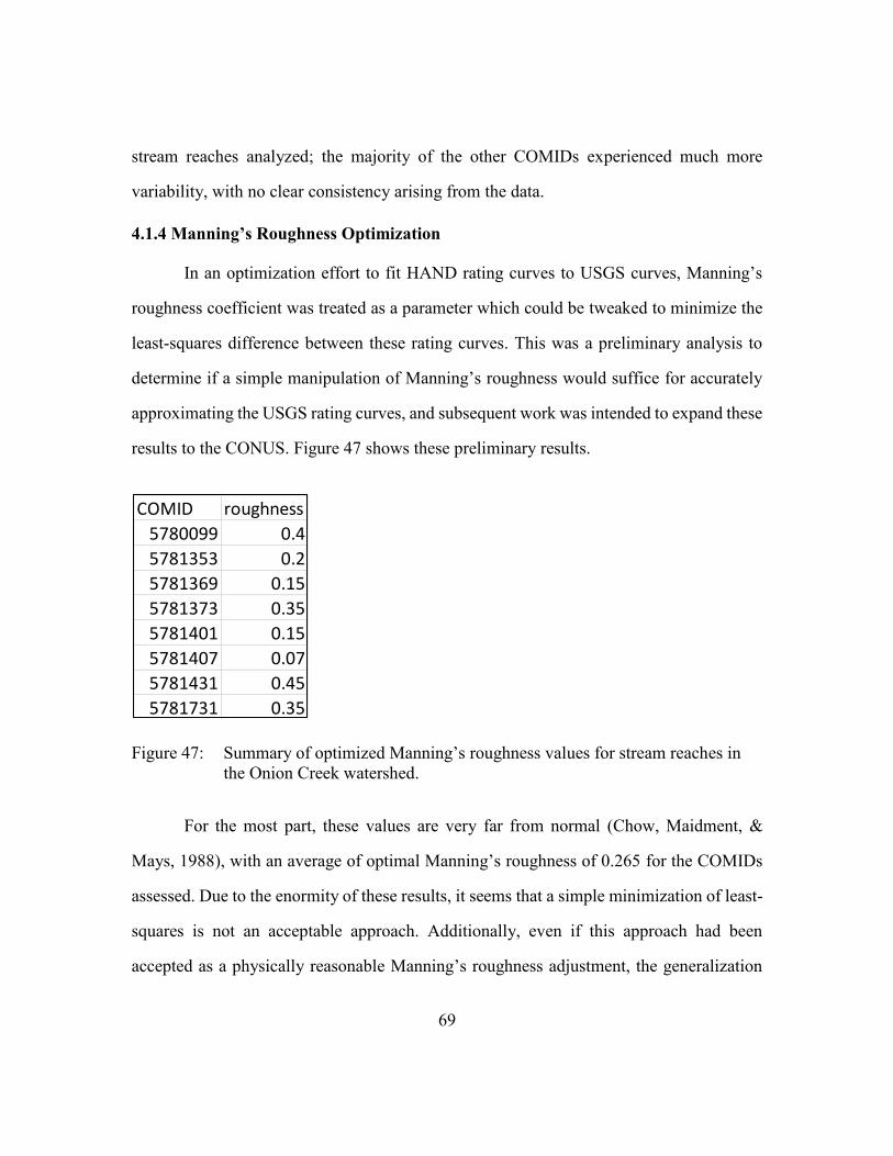
69

stream reaches analyzed; the majority of the other COMIDs experienced much more

variability, with no clear consistency arising from the data.

4.1.4 Manning’s Roughness Optimization

In an optimization effort to fit HAND rating curves to USGS curves, Manning’s

roughness coefficient was treated as a parameter which could be tweaked to minimize the

least-squares difference between these rating curves. This was a preliminary analysis to

determine if a simple manipulation of Manning’s roughness would suffice for accurately

approximating the USGS rating curves, and subsequent work was intended to expand these

results to the CONUS. Figure 47 shows these preliminary results.

Figure 47: Summary of optimized Manning’s roughness values for stream reaches in

the Onion Creek watershed.

For the most part, these values are very far from normal (Chow, Maidment, &

Mays, 1988), with an average of optimal Manning’s roughness of 0.265 for the COMIDs

assessed. Due to the enormity of these results, it seems that a simple minimization of least-

squares is not an acceptable approach. Additionally, even if this approach had been

accepted as a physically reasonable Manning’s roughness adjustment, the generalization

COMID roughness

5780099 0.4

5781353 0.2

5781369 0.15

5781373 0.35

5781401 0.15

5781407 0.07

5781431 0.45

5781731 0.35

70

of this solution to a national scale would have been remarkably difficult; there are simply

not enough USGS gages to create a meaningful machine learning training dataset from (let

along validation and testing datasets).

4.2 CROSS SECTIONS

Interesting comparisons between HAND and USGS cross sections were also

conducted, such as that shown in Figure 48. This comparison looks fairly good, reinforcing

the belief that the HAND methodology is consistently missing some area at the bottom of

each cross-section (see right side of Figure 48, with GZF depth correction implemented).

As is also clear from this comparison, the GZF shift is necessary for any sort of meaningful

comparison between HAND and USGS cross-sections, because without this shift the cross-

sections do not relate in any visibly meaningful way (as in the case of the left image in

Figure 48).

Figure 48: HAND (blue) and USGS (green) cross sections with (left) and without

(right) a GZF depth shift correction for COMID 5781369.

Due to this restriction, and due to the lack of available GZF shift data for the stream

reaches here in question, there are few cross section results, most of which look worse than

71

that shown in Figure 48. Many results have cross sections that are tens of feet separated

due to unavailable depth shifts or other complications. As such, no HAND rating curve

recommendations can be recommended based on these cross sections.

4.3 FINAL RATING CURVES

Analyzed over the revised study area and using the more complex HEC-RAS reach-

averaged rating curves for comparison, this final analysis summarizes a meaningful way to

compare the various options presented.

4.3.1 Rating Curves

A visual assessment of fit was first used to determine which combination of

roughness and slope correction methodologies would result in the best HAND rating curves

(as compared to the median HEC-RAS rating curves) for Onion Creek as a whole. An

example visualization is shown in Figure 49, comparing different roughness alternatives

with NHDPlusV2 or DEM-derived catchment-averaged slopes. The nearest-neighbor

slopes are not shown on this particular plot to avoid clutter, but they can be analyzed in a

similar way as well.

72

Figure 49: Example of various HAND-derived rating curves as compared to the HEC-

RAS rating curve and its power-law fit curve for COMID 5781369.

While it is clear that the best curves for this reach are either the DEM-derived slope

with the NLCD-based roughness-by-depth approach, or the DEM-derived slope with a

reach-averaged NLCD-based roughness, this is not consistent when compared amongst all

stream reaches. As such, a least-squares approach was used to assess performance,

assessing which approach minimized the least-squares difference for a majority of the

stream reaches along Onion Creek.

4.3.2 Least-Squares Difference Analysis

In order to conduct a least-squares difference minimization, first a multitude of data

points must be gathered along the curves to be compared. The HAND rating curves have

83 data points, one for each whole number stage height between 0 and 82 feet, whereas the

HEC-RAS rating curves have only eight evenly-spaced data points at decimal stage heights

73

along the curve. Therefore, in enabling a comparison between these two curves, a power-

law curve was first fit to each HEC-RAS rating curve to enable queries upon it at all 1-foot

stage height intervals.

Using power-law curves fitted to each catchment’s averaged HEC-RAS rating

curve, a more mathematically meaningful comparison of least-squares differences could

be made between the median HEC-RAS rating curve and various HAND-derived rating

curves. Notably, these power-law fits did not always perfectly describe the rating curves

they were derived from. An example of a very good fit and one of the worst fits within

Onion Creek are shown in Figure 50; most rating curves fell somewhere on the spectrum

between these two examples in terms of goodness of fit. This introduces some error into

the least-squares difference methodology here applied, yet this power-law fit was still

considered to be superior as compared to the linear interpolation seen in red in Figure 50,

particularly seeing as the power-law fit fairly accurately describes the lower stage heights

of the rating curve, while the linear interpolation shortcuts this portion of the curve.

Figure 50: Two example HEC-RAS rating curves showing a power-law curve fitted to

the eight linearly-interpolated HEC-RAS data points. COMID 5781411

(left) shows an exceptionally good fit, while COMID 5781403 (right) shows

a relatively poor fit.

74

Once the HEC-RAS rating curves were fit to a power-law function, squared

discharge differences were summed for all 1-foot stage height intervals up to the final

HEC-RAS data point; this distinction is important, as it removed the errors that would be

experienced as the power-law curves approached infinite discharges for marginally larger

stage heights. This least-squares difference approach was then applied for all potential

HAND rating curves as compared to a stream reach’s power-law fit HEC-RAS rating

curve. These least-squares differences were then ranked for each COMID, resulting in an

ordering as shown in Figure 51.

Figure 51: Organization of least-squares difference from best to worst HAND rating

curve candidate for each COMID along Onion Creek.

From Figure 51, it is fairly clear that, when paired with the depth shift and some

form of slope adjustment, the NLCD roughness by depth (“nlcdroughbydepth”)

methodology is an improvement over the 0.05 Manning’s roughness assumption

previously used. While these changes to the Manning’s roughness seem to consistently

improve results, understanding which slope is the best performer is more difficult. In the

“Best” column, seven of thirteen results show the DEM-derived slope as being the winner.

However, seeing as this represents only 54% of a very small sample, the second-best

column was also assessed, showing that the NHDPlusV2 slope seems superior overall. This

discrepancy creates some confusion and fails to inform any valid conclusions.

75

In a more useful visualization, box plots were generated to explore the spread of

least-squares values when assessing all catchments along Onion Creek (see Figure 52,

where the y-axis represents the least-squares differences in trillion cubic feet per second;

smaller values correspond to minimal least-squares differences). Plotting only catchment-

averaged slopes, the NHDPlusV2 catchment-averaged slope and the NLCD roughness by

depth approaches together seemed to minimize the deviations of the rating curve least-

squares differences significantly more than the other methods. Notably, as mentioned, each

least-squares regression was computed only up to the furthest HEC-RAS point for each

stream-reach to avoid extreme power-curve deviation at larger stage-heights. This resulted

in least-squares values likely deviating in magnitude from reach to reach, which may have

caused some of the extreme outliers shown in Figure 52. However, because this value was

consistent for all methodologies for any given reach (because this cut-off is based on the

HEC-RAS rating curve, not the HAND rating curve), this difference was deemed to be

acceptable.

76


COMIDs organized by rating curve adjustment type.

While conclusive results as to the best of the six methods may or may not be valid,

it is fairly clear that the NLCD roughness adjustments tend to outperform the original 0.05

roughness assumption for both slope alternatives. The comparison is still unclear as to

slope performance, but the NHDPlusV2 slopes seem to perform best.

In remembering that COMID 5781939 was a problematic reach with a miniscule

(NHDPlusV2) or zero (DEM-derived) slope, this particular reach was treated as an outlier

and was temporarily removed from the analysis. After ignoring COMID 5781939, the

resulting performance of the Onion Creek catchments significantly improved (see Figure

77

53), showing that, if this problematic reach is ignored, the NLCD roughness by depth

approach seems to be the clear winner over the other approaches. While the DEM-derived

slope seems to perform marginally better than the NHDPlusV2 slopes overall, the

conclusion as to which is the better approach remains unclear.


COMIDs excluding COMID 5781939.

In attempting to resolve these slope complications, the previously-calculated

catchment-averaged and nearest-neighbor slopes were used in conjunction with the NLCD-

based roughness by depth approach to generate a new set of box plots strictly comparing

78

the influence of different slopes (see Figure 54). COMID 5781939 was added back in again

for this analysis, as the real purpose of this project is to determine a generalizable approach

for resolving all rating curve corrections. As such, even the problematic reaches need to be

included.


COMIDs, specifically comparing various slope alternatives. The NLCD

roughness by depth approach is used for all of these box plot alternatives.

From this comparison, the NHDPlusV2 reach-averaged slope is clearly the best

performer. However, despite this improved performance, the nearest-neighbor approach

79

would likely be the simplest to generalize and implement on a large scale. Consequently,

the NHDPlusV2 nearest-neighbor slope is considered to be the best all-around performer,

though further research is highly recommended before adapting these changes.

80

Chapter 5: Conclusions

A major finding of this research is that, while USGS rating curves are largely

beneficial for spot-checking of models at specific locations, they are largely ineffective for

national-scale flood mapping due to their relative spatial scarcity. Consequently, while

precisely-derived rating curves from highly detailed cross section field measurements may

be beneficial to small-scale studies, they should not be relied upon for large-scale

hydrological implementations. In the end, a generalizable flood extent modeling approach

that is mostly correct and operational is vastly preferable to a system that is perpetually

being improved and never being delivered.

An additional finding from HEC-RAS rating curve exploration is also interesting.

HEC-RAS rating curves along each NHDPlusV2 stream reach have much more resolution

than the more sparse USGS rating curves. Consequently, if a method existed to ingest all

HEC-RAS models throughout the nation for detailed river channel modeling, then the

NHDPlusV2 stream reaches might all feasibly be highly understood in the near future.

Similarly, if the theoretical reasons for at-a-station hydraulic geometry relations are ever

agreed upon, cross section geometries may be computed at a very high spatial scale.

However, while this may sound very interesting from a hydrological perspective, it has

here been discovered that an incredibly high level of detail may in fact be disadvantageous.

The large quantity of HEC-RAS rating curves had such an enormous spread for each

NHDPlusV2 stream reach (and this spread was consistently large, even for smaller subsets

of these stream reaches) that averaging these rating curves over the entire stream reach was

the only feasible method for utilizing them. Ironically, an excess of data is also seemingly

unbeneficial.

81

A third and very important finding is that both the NHDPlusV2 and DEM-based

slopes utilized in this analysis were found to be unreasonable for Onion Creek. The

tremendous amount of variation occurring along this one reach, as well as the fairly

common zero-slope reaches (or 0.00001 m/m for NHDPlusV2), is hydrologically and

bathymetrically unlikely. From the Onion Creek stream profile generated in this research,

it is apparent that the HEC-RAS model has a significantly more consistent (and realistic)

understanding of bed elevation which is not captured by the National Elevation Dataset.

An alternative methodology is likely needed to resolve this issue, with nearest-neighbor

averages presenting a possible step in the correct direction.

Regarding the extensive analysis of different proposed solutions for improving

HAND rating curves, it is clear that some newly-proposed approaches may be

advantageous. In particular, the NLCD roughness by depth approach seems to improve

Onion Creek rating curves significantly on average. Similarly, while the results were not

nearly as conclusive, the NHDPlusV2 slopes seem preferable to the DEM-derived slopes,

and the problem of tremendously small slope values can possibly be decreased through

nearest-neighbor slope averaging.

While these results seem to have clear benefits to national-scale HAND rating curve

improvements, their exploration at the Onion Creek scale are insufficient for large scale

implementation. To further this research, these findings must be explored for other stream

reaches, preferably in other regions with different climates, topologies, and geographies

than those present in Onion Creek. Finally, if certain approaches seem to consistently

improve HAND rating curves across regions, a full analysis must take place at the national

scale, including all 2.67 million NHDPlusV2 stream reaches, before implementation of

these new methodologies should be applied.

82

Though the purpose of this research was to improve the process of generating

HAND rating curves on a national scale, many incompatible approaches ended up

becoming the most informative findings. From limited USGS data availability and

extensive HEC-RAS data availability, the NHDPlusV2 stream reach-averaged rating curve

approach was very much validated; this level of resolution is ideal for the implementation

of flood extent mapping using current technologies. Additionally, potential solutions

relying on other national datasets have been explored, particularly the NLCD roughness

approaches and the DEM-derived slopes, which both seem to present feasible results that

are easily generalizable at the national scale. The HAND predictive flood extent

methodology is on the verge of implementation. Hopefully these proposed improvements

can further this research, helping to save lives nationwide.

83

References

Asquith, W. H. & Roussel, M. H. 2009. Regression Equations for Estimation of Annual

Peak-Streamflow Frequency for Undeveloped Watersheds in Texas Using an L-

moment-Based, Press-Minimized, Residual-Adjusted Approach. U.S. Geological

Survey Scientific Investigations Report 2009-5087. Retrieved from:

https://pubs.usgs.gov/sir/2009/5087/pdf/sir2009-5087.pdf

Austin American-Statesman. n.d. History of Onion Creek Flooding. Retrieved from:

http://www.statesman.com/news/history-onion-creek-

flooding/R6y769kkhg4bo5ZtiesVUM/

Braca, Giovanni, & Futura, Grafiche. 2008. Stage-Discharge Relationships in Open

Channels: Practices and Problems. Trento University. Department of Civil and

Environmental Engineering.

Brunner, G. W. 2016. HEC-RAS River Analysis System User’s Manual Version 5.0. US

Army Corps of Engineers, Hydrologic Engineering Center. Retrieved from:

http://www.hec.usace.army.mil/software/hec-ras/documentation/HEC-

RAS%205.0%20Users%20Manual.pdf

Chow, V. T., Maidment, D. R., Mays, L. W. 1988. Applied Hydrology.

Chow, Ven. 1953. Open-Channel Hydraulics. Civil Engineering Series. The University of

Michigan: McGraw-Hill.

City of Austin. n.d. Austin FloodPro. http://www.austintexas.gov/FloodPro/

Cosgrove, B. & Klymmer, C. 2016. National Water Model. Retrieved from:

http://water.noaa.gov/about/nwm

Dingman, S. L. 2007. Analytical Derivation of At-a-station Hydraulic-Geometry Relations.

Journal of Hydrology 334. DOI: http://dx.doi.org/10.1016/j.jhydrol.2006.09.021

Fagan, C. 2016. Improving Flood Preparedness in South-Central Texas. MA Thesis,

University of Texas at Austin. Retrieved from:

https://repositories.lib.utexas.edu/bitstream/handle/2152/38755/FAGAN-

THESIS-2016.pdf?sequence=1

Federal Emergency Management Agency (FEMA). 2013. NGVD NAVD? Retrieved

from: https://www.fema.gov/media-library-data/20130726-1755-25045-

0634/ngvd_navd.pdf

Federal Emergency Management Agency (FEMA). n.d. Flood Map Service Center.

Retrieved from: https://msc.fema.gov/portal/

Ferguson, R. 1986. Hydraulic and hydraulic geometry. Progress in Physical Geography 10,

1-31.

http://www.statesman.com/news/history-onion-creek-flooding/R6y769kkhg4bo5ZtiesVUM/

http://www.statesman.com/news/history-onion-creek-flooding/R6y769kkhg4bo5ZtiesVUM/

http://dx.doi.org/10.1016/j.jhydrol.2006.09.021

https://www.fema.gov/media-library-data/20130726-1755-25045-0634/ngvd_navd.pdf

https://www.fema.gov/media-library-data/20130726-1755-25045-0634/ngvd_navd.pdf

84

Gharari, S., Hrachowitz, M., Fenicia, F., & Savenije, H. H. G. 2011. Hydrological

Landscape Classification: Investigating the Performance of HAND Based

Landscape Classifications in a Central European Meso-Scale

Catchment. Hydrology and Earth System Sciences, 15(11), 3275-3291. Retrieved

from: http://www.hydrol-earth-syst-sci.net/15/3275/2011/hess-15-3275-2011.pdf

Gleason, C. J. 2015. Hydraulic geometry of natural rivers: A review and future

directions. Progress in Physical Geography, 39(3), 337-360.

Hernandez, W. J., Armstrong, R. A. 2016. Deriving Bathymetry from Multispectral

Remote Sensing Data. Journal of Marine Science and Engineering, 4(1), 8.

Retrieved from:

https://pdfs.semanticscholar.org/cef7/4efb22f8e51b17e16c51f3a1802b1041a561.p

df

Homer, C.G., Dewitz, J.A., Yang, L., Jin, S., Danielson, P., Xian, G., Coulston, J., Herold,

N.D., Wickham, J.D., & Megown, K. 2015. Completion of the 2011 National Land

Cover Database for the Conterminous United States – Representing a Decade of

Land Cover Change Information. Photogrammetric Engineering and Remote

Sensing, v. 81, no. 5, p. 345-354

Johnson, M., Ruess, P., & Coll, J. 2016. OPERA – Operational Platform for Emergency

Awareness: Reimagining Disaster Alerts. Ch. 13. Consortium of Universities for

the Advancement of Hydrologic Sciences, Inc. DOI:

http://dx.doi.org/10.4211/technical.20161019

Leopold, L. and T. Maddock 1953. The hydraulic geometry of stream channels and some

physiographic implications. Geological Survey professional paper 252, 1-56.

Liu, Y. et al. 2016. A CyberGIS Approach to Generate High-Resolution Height Above

Nearest Drainage (HAND) Raster for National Flood Mapping. Retrieved from:

http://www.cigi.illinois.edu/yanliu/NFIEHAND.pdf

Liu, Y. Y., Maidment, D. R., Tarboton, D. G., Zheng, X., & Wang, S. W. 2017. A

CyberGIS Integration and Computation Framework for High-Resolution

Continental-Scale Flood Inunundation Mapping. Journal of the American Water

Resources Association (JAWRA). Draft for review.

Maidment, D. R. 2016. Conceptual Framework for the National Flood Interoperability

Experiment. Journal of the American Water Resources Association. Retrieved

from:

https://www.cuahsi.org/Files/Pages/documents/13623/nfieconceptualframework_r

evised_feb_9.pdf

Manning, R. 1891. On the Flow of Water in Open Channels and Pipes. Transactions of the

Institution of Civil Engineers of Ireland. 20. 161-207

Manning, R. 1895. On the Flow of Water in Open Channels and Pipes – Supplement to a

Paper Read on the 4th December 1889, published in the Transactions, 1891, vol.

http://bit.ly/1K7WjO3



http://dx.doi.org/10.4211/technical.20161019

85

XX, p. 161. Transactions of the Institution of Civil Engineers of Ireland, 24, 179-

207

Mckay, L., Bondelid, T., Dewald, T., Johnston, J., Moore, R., & Rea, A. 2012. NHDPlus

Version 2: User Guide. Horizon Systems Corporation. Retrieved from:

ftp://ftp.horizon-

systems.com/nhdplus/NHDPlusV21/Documentation/NHDPlusV2_User_Guide.pd

f

Moore, M. R. 2011. Development of a High-Resolution 1D/2D Flood Simulation of

Charles City, Iowa. MS Thesis, University of Iowa. Retrieved from:

http://ir.uiowa.edu/cgi/viewcontent.cgi?article=2417&context=etd

National Flood Interoperability Experiment (NFIE). n.d. Index of /nfiedata/.

http://nfie.roger.ncsa.illinois.edu/nfiedata/

National Oceanic and Atmospheric Administration (NOAA). 2016. NOAA Launches

America’s First National Water Forecast Model. Retrieved from:

http://www.noaa.gov/media-release/noaa-launches-america-s-first-national-water-

forecast-model

National Water Model (NWM) Forecast Viewer. 2016. Hydroshare. Retrieved from:

https://apps.hydroshare.org/apps/nwm-forecasts/

National Weather Service (NWS). 2016. Natural Hazards Statistics. Retrieved from:

http://www.nws.noaa.gov/om/hazstats.shtml

National Weather Service (NWS). n.d. National Forecasts: River Forecasts. Retrieved

from: https://water.weather.gov/ahps/forecasts.php

Nobre, A. D. 2011. Height Above the Nearest Drainage – A Hydraulically Relevant New

Terrain Model. Journal of Hydrology, 404.1-2, pp. 13-29. DOI:


Park, C. C. 1977. World-wide variations in hydraulic geometry exponents of stream

channels: An analysis and some observations. Journal of Hydrology, 33, 133-146

Parker, G. 1979. Hydraulic Geometry of active gravel rivers. Journal of Hydraulic Division

105, 1185-1201.

Raymond, P. A. 2012. Scaling the Gas Transfer Velocity and Hydraulic Geometry in

Streams and Small Rivers. Journal of Hydrology, 2.1, pp. 41-53. DOI:

http://dx.doi.org/10.1215/21573689-1597669

Reistad, K. S., Petersen-Øverleir, A., Bogetveit, L. J. 2005. Setting up Rating Curves Using

HEC-RAS. Retrieved from:

https://www.researchgate.net/publication/265166848_Setting_up_rating_curves_u

sing_HEC-RAS


http://dx.doi.org/10.1215/21573689-1597669

https://www.researchgate.net/profile/Asgeir_Petersen-Overleir

86

Rennó, C. D., Nobre, A. D., Cuartas, L. A., Soares, J. V., Hodnett, M. G., Tomasella, J., &

Waterloo, M. J. 2008. HAND, a New Terrain Descriptor Using SRTM-DEM:

Mapping Terra-Firme Rainforest Environments in Amazonia. Remote Sensing of

Environment, 112(9), 3469-3481. Retrieved from:

http://www.dpi.inpe.br/referata/arq/_2012/12_Gabriel/Renno_etal_2008.pdf

Rhodes, D. D. 1977. The b-f-m diagram: Graphical representation and interpretation of at-

a-station hydraulic geometry. Amercian Journal of Science 277, 73-96

Rhodes, D. D. 1987. The bfm diagram for downstream hydraulic geometry. Geografiska

Annaler. Series A. Physical Geography, 147-161.

Sauer, V. B. 2002. Standards for the Analysis and Processing of Surface-Water Data and

Information using Electronic Methods (No. 2001-4044). United States Geological

Survey

Seaber, P. R., Kapinos, F. P., and Knapp, G. L. 1987. Hydrologic Unit Maps. U.S.

Geological Survey Water-Supply Paper 2294. Retrieved from:

https://pubs.usgs.gov/wsp/wsp2294/pdf/wsp_2294_a.pdf

Smith, L. C., Pavelsky, T. M. 2008. Estimation of River Discharge, Propagation Speed,

and Hydraulic Geometry from Space: Lena River, Siberia. Water Resources

Research 44.3. DOI: http://dx.doi.org/10.1029/2007WR006133

Tarboton, D. G., Idaszak, R., Horsburgh, J. S., Heard, J., Ames, D., Goodall, J. L., ... &

Hooper, R. 2014. HydroShare: advancing collaboration through hydrologic data

and model sharing. Retrieved from:

http://scholarsarchive.byu.edu/cgi/viewcontent.cgi?article=1005&context=iemssc

onference

United States Geological Survey (USGS). n.d. Water Watch. Retrieved from:

http://waterwatch.usgs.gov

Wahlstrom, M., and Guha-Sapir, D. 2015. “The Human Cost of Weather-Related Disasters

1995-2015.” Geneva, Switzerland: UNISDR (2015). Retrieved from:

http://www.preventionweb.net/publications/view/46796

Whiteaker, T. 2016. PyNWM. Github Repository. Retrieved from:

https://github.com/twhiteaker/pynwm

Zheng, X. 2015. Hydraulic Fabric: An Information Framework for River Channel Cross

Section Data. MS Thesis, University of Texas at Austin. Retrieved from:

http://hdl.handle.net/2152/31786

Zheng, X., Tarboton, D., Maidment, D., Liu, Y., Passalacqua, P. 2017. River Channel

Geometry and Rating Curve Estimation Using Height Above the Nearest Drainage.

Manuscript in preparation.

http://dx.doi.org/10.1029/2007WR006133

http://waterwatch.usgs.gov/

http://www.preventionweb.net/publications/view/46796

87

Vita

Paul Ruess grew up in Northern Virginia, just outside of Washington, D.C. After

receiving a Bachelor of Science degree in Civil and Environmental Engineering from the

University of Virginia, Paul began a professional career as a wastewater engineer. Paul

then moved to Austin one year later to pursue a Master of Science degree in Environmental

and Water Resources Engineering. Following graduation, Paul intends to begin a PhD

program at the University of Illinois Urbana-Champaign, where he will investigate the

Food-Energy-Water Nexus.

Permanent email: [email protected]

This thesis was typed by Paul Joseph Ruess.

copyright by paul joseph ruess 2017

Documents