copyright by runhua guo 2007
TRANSCRIPT

Copyright
by
Runhua Guo
2007
This Dissertation Committee for Runhua Guo certifies that this is the approved version of the following dissertation:
PREDICTING IN-SERVICE FATIGUE LIFE OF FLEXIBLE
PAVEMENTS BASED ON ACCELERATED PAVEMENT TESTING
Committee:
__________________________ Jorge A. Prozzi, Supervisor
__________________________ Randy B. Machemehl
__________________________ C. Michael Walton
__________________________ Kevin J. Folliard
__________________________ Harovel G. Wheat
PREDICTING IN-SERVICE FATIGUE LIFE OF FLEXIBLE
PAVEMENTS BASED ON ACCELERATED PAVEMENT TESTING
by
Runhua Guo, B.S., M.S.
Dissertation
Presented to the Faculty of the Graduate School of
The University of Texas at Austin
in Partial Fulfillment
of the Requirements
for the Degree of
Doctor of Philosophy
The University of Texas at Austin
December 2007

To my family for their unconditional love and support,
To my Xiao-tu-di and Zao-zao

ACKNOWLEDGEMENTS
I wish to express my deepest appreciation to my dissertation supervisor, Dr. Jorge A.
Prozzi and Ms. Jolanda Prozzi, for all of the support and mentorship that they have
provided me during my time here at the University of Texas at Austin. It has been an
honor, a pleasure, and a blessing to have the opportunity to work with them.
I would like to thank my committee member Randy B. Machemehl, Kevin J.
Folliard, C. Michael Walton, and Harovel G. Wheat for their insights and valuable
suggestions to this work. The author also is very grateful to Darhao Chen for his
provision of data and other support. My special thanks go to Janet A Slack for all of the
assistance she provided during these years.
The discussions with Feng Hong, Feng Wang, Zhong Wang, Bin Zhou, Jianming
Ma, Zheng Li, Xiaokun Wang, Lu Gao, Hui Wu, Jessica Y. Guo, Isabel Victoria and Jose
Pablo Aguiar-Moya are helpful and should be credited. My special thanks also go to
Huimin Zhao and Yong Zhao for the precious friendship and for their sincere and
generous support.
Last but not least, I am indebted to my wife Hangwen Liang, my parents Zhonghe
Guo and Shifeng Yang, my parents-in-law Xueti Liang and Xiafang Yu, my brother
Yaping Guo, my brother Yaqun Guo, my sister Yali Guo, my brother-in-law Tinghui Xu,
my sister-in-law Xuemei Li, and my sister-in-law Chunxia Wang. Without their support
and encouragement, I would never finish this work. I shall make it up to them during my
lifetime.
v
PREDICTING IN-SERVICE FATIGUE LIFE OF FLEXIBLE
PAVEMENTS BASED ON ACCELERATED PAVEMENT TESTING
Publication No._____________
Runhua Guo, Ph.D.
The University of Texas at Austin, 2007
Supervisor: Jorge A. Prozzi Pavement performance prediction in terms of fatigue cracking and surface rutting are
essential for any mechanistically-based pavement design method. Traditionally, the
estimation of the expected fatigue field performance has been based on the laboratory
bending beam test. Full-scale Accelerated Pavement Testing (APT) is an alternative to
laboratory testing leading to advances in practice and economic savings for the evaluation
of new pavement configurations, stress level related factors, new materials and design
improvements. This type of testing closely simulates field conditions; however, it does
not capture actual performance because of the limited ability to address long-term
phenomena. The same pavement structure may exhibit different response and
performance under APT than when in-service. Actual field performance is better captured
by experiments such as Federal Highway Administration’s Long-Term Pavement
vi

Performance (LTPP) studies. Therefore, to fully utilize the benefits of APT, there is a
need for a methodology to predict the long-term performance of in-service pavement
structures from the results of APT tests that will account for such differences. Three
models are generally suggested to account for the difference: shift factors, statistical and
mechanistic approaches.
A reliability based methodology for fatigue cracking prediction is proposed in this
research, through which the three models suggested previously are combined into one
general approach that builds on their individual strengths to overcome some of the
shortcomings when the models are applied individually. The Bias Correction Factor
(BCF) should account for all quantifiable differences between the fatigue life of the
pavement site under APT and in-service conditions. In addition to the Bias Correction
Factor, a marginal shift factor, M, should be included to account for the unquantifiable
differences when predicting the in-service pavement fatigue life from APT.
The Bias Correction Factor represents an improvement of the currently used “shift
factors” since they are more general and based on laboratory testing or computer
simulation. By applying the proposed methodology, APT performance results from a
structure similar to an in-service structure can be used to perform four-point bending
beam tests and structural analysis to obtain an accurate estimate of the necessary Bias
Correction Factor to estimate in-service performance.
vii
Table of Contents
List of Figures.....................................................................................................................x
List of Tables....................................................................................................................xii
Chapter 1: Introduction................................................................................................... 1
1.1 Background................................................................................................................... 1
1.2 Problem Statement........................................................................................................ 3
1.3 Research Objective....................................................................................................... 5
1.4 Organization of Dissertation........................................................................................ 6
Chapter 2: Literature Review ........................................................................................ 8
2.1 Overview...................................................................................................................... 8
2.2 Fatigue Test of Asphalt Mixtures .............................................................................. 12
2.3 Fatigue Characteristics of Asphalt Mixtures............................................................... 22
2.4 Accelerated Pavement Testing………........................................................................ 26
Chapter 3: Methodology................................................................................................. 35
3.1 Principles of Methodology.......................................................................................... 35
3.2 Methods and Procedures............................................................................................. 39
3.3 Reliability-based Fatigue Performance Prediction .................................................... 41
Chapter 4: Gathering and Processing of Performance Data...................................... 45
4.1 Accelerated Pavement Testing in California ............................................................. 45
4.2 Federal Highway Administration’s Accelerated Loading Facility............................. 48
4.3 Performance Data for In-service Flexible Pavement.................................................. 49
Chapter 5: Development of the Bias Correction Factor ............................................. 53
5.1 Bias Correction Function for Temperature and Loading Speed (frequency) ............ 55
5.2 Bias Correction Function for Traffic Wandering ....................................................... 64
5.3 Bias Correction Function for Moisture ...................................................................... 67
5.4 Bias Correction Function for Loading Ratio ............................................................. 67
5.5 Sensitivity Analysis of Bias Correction Functions..................................................... 70
viii
Chapter 6: Reliability Based Fatigue Life Prediction................................................. 75
6.1 Test Results of Bias Correction Functions................................................................. 75
6.2 Marginal Shift Factor (m)........................................................................................... 86
6.3 Reliability Based Fatigue Life Prediction................................................................... 90
Chapter 7: Validation of the Fatigue Life Prediction.................................................. 92
7.1 Principles of Validation.............................................................................................. 92
7.2 Data Gathering and Processing................................................................................... 93
7.3 Verification and Validation Analysis of the Proposed Fatigue Life Prediction.........97
Chapter 8: Summary, Conclusions and Future Work...............................................101
8.1 Summary....................................................................................................................101
8.2 Conclusions ...............................................................................................................102
8.3 Methodology Limitations and Further Research...................................................... 106
Appendix A: Specification of the Bias Correction Functions....................................107
Appendix B: Estimation of Correlation Matrix for the Parameters in Fatigue Life
Prediction.................................................................................................................112
Appendix C: Laboratory Fatigue Tests.......................................................................115
Appendix D: Sensitivity Analysis of the Model Parameters on the Predicted Fatigue
Life of Flexible Pavements.....................................................................................133
List of References..........................................................................................................135
Vita..................................................................................................................................146
ix

List of Figures
Figure 1.1 Interrelationship between pavement engineering facets (Hugo et al., 1991)….2
Figure 3.1 Main differences between in-service and APT fatigue performance………...36
Figure 3.2 Estimation of field performance: F′ = A × B × M……………………………37
Figure 3.3 Reliability statement of performance prediction from APT………………….43
Figure 4.1 Structural pavement sites of CAL/APT program (Harvey et al., 1999) ……..46
Figure 4.2 Performance fatigue data corresponding to 6 subsections of site 501RF…….47
Figure 4.3 Performance fatigue data corresponding to 6 subsections of site 503RF…….47
Figure 4.4 Layout of the pavement lanes for fatigue tests ………………………………48
Figure 4.5 Percentage of area cracked corresponding to 9 fatigue test sites…………….49
Figure 5.1 Four-point bending fatigue testing apparatus ………………………………..56
Figure 5.2 Mode for loading speed (frequency) calculation……………………………..58
Figure 5.3 Master curve of a particular asphalt mixture…………………………………61
Figure 5.4 Traffic loading with or without rest period…………………………………..68
Figure 5.5 Effect of temperature on BCFs……………………………………………….71
Figure 5.6 Effect of driving speed on BCFs……………………………………………..72
Figure 5.7 Effect of subgrade modulus change on BCFs………………………………..72
Figure 5.8 Effect of loading ratio on BCFs………………………………………………73
Figure 5.9 Effect of standard deviation of lateral position on BCFs…………………….74
Figure 6.1 Hourly temperature change of LTPP site 48-6160 in different month……….75
Figure 6.2 Hourly pavement temperature change of LTPP site 48-6160 at different
depth………………………………………………………………………………...76
Figure 6.3 Sinusoidal curve fitted to hourly air temperature…………………………….77
Figure 6.4 A ten-year air temperature record of LTPP site 48-6160…………………….78
Figure 6.5 Estimated annual average daily number of trucks in the LTPP lane…………81
Figure 6.6 Definition of a fully damaged fatigue cracking area…………………………86
(DR=1, crack density = 6.7m/m2 correspondingly)
x
Figure 6.7 Constrained regressions on marginal shift factor M…………………………88
Figure 6.8 Histogram of log (εi) …………………………………..…………………….90
Figure 6.9 Probability plot of log (εi) ………………………………………..………….91
Figure 7.1 Layout of part of the 12 pavement test lanes……………………..………….94
Figure 7.2 Performance fatigue data corresponding to Lane 2 site 3 (PG70-22) ……….94
Figure 7.3 LTPP sites selected for approach validation………………………….……..96
Figure 7.4 Plot of observed vs. predicted number of ESALs……….………………....99
xi

List of Tables
Table 4.1 Selected LTPP sites match CAL/APT program………………………………51
Table 4.2 Selected LTPP sites match FHWA/ALF program……………………………51
Table 5.1 Loading frequencies at different speed and load spread area width (Hz) ……59
Table 5.2 Experimental arrangement of fatigue tests……………………………………60
Table 5.3 Laboratory four-point bending fatigue test results……………………………62
Table 5.4 Regression analysis of temperature and loading frequency…………………..63
Table 5.5 Regression analysis of loading ratio based on laboratory investigation………69
Table 6.1 BCFs of LTPP sites to different APT temperatures…………………………..79
Table 6.2 BCFs of LTPP sites to different APT loading speed………………………….80
Table 6.3 Hour truck traffic distribution default values based on LTPP traffic data
(NCHRP, 2006) …………………………………………………………………… 81
Table 6.4 BCFs of LTPP sites to different APT loading ratio…………………………...82
Table 6.5 Maximum tensile strains in the asphalt layer matched with CAL/APT………84
Table 6.6 Maximum tensile strains in the asphalt layer matched with FHWA/ALF Lane
1&2 (10^-6)……………….…………………………………………………………84
Table 6.7 Maximum tensile strains in the asphalt layer matched with FHWA/ALF Lane
3&4 (10^-6)…………….………………………………………………………….. 85
Table 6.8 Summary table of Bias Correction Functions…………………………………85
Table 6.9 Load repetitions (in ESALs) of LTPP and APT at different DR…...…………89
Table 6.10 Standard normal deviate for various levels of reliability………….…………91
Table 7.1 Selected LTPP sites match FHWALF program………….………………….97
Table 7.2 Summary table of the fatigue life prediction………….………………….....98
Table 7.3 Summary statistics for the measured and predicted traffic………….….…....99
xii
Chapter 1: Introduction
1.1 Background
Pavement performance prediction in terms of fatigue cracking and surface rutting is
essential for any mechanistically-based pavement design method (NCHRP, 2006). The
estimation of the expected fatigue performance of a flexible pavement in the field is
based on the estimation of the maximum tensile strain at the bottom of the asphalt layers
and its correlation to the performance of the same mix in the laboratory under bending
beam test. This laboratory-based estimation is further calibrated to better predict actual
field performance by means of shift factors (Al-Qadi and Nassar, 2003). But none of
these shift factors have been comprehensive and often are limited to assessing the effect
of one variable at a time.
Full-scale Accelerated Pavement Testing (APT) is a supplement to laboratory testing.
It is defined as the controlled application of a prototype wheel loading, at or above loads
representative of field traffic loads to a prototype or actual, layered, structural pavement
system to determine pavement response and performance under a controlled, accelerated
accumulation of damage in a compressed time period (Metcalf, 1996). There are a wide
variety of APT programs in operation today. Metcalf indicated that 35 full scale APT
facilities existed worldwide in 1996, of which 19 had active research programs. By 2004,
28 such programs were reported as being active, among which more than half are in the
1
United States (Hugo and Epps, 2004). Therefore, a globally scaled knowledge exists in
the field of APT. As a facet of pavement engineering, APT generates knowledge over a
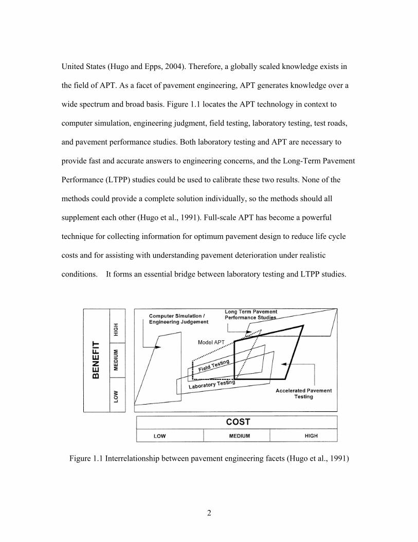
wide spectrum and broad basis. Figure 1.1 locates the APT technology in context to
computer simulation, engineering judgment, field testing, laboratory testing, test roads,
and pavement performance studies. Both laboratory testing and APT are necessary to
provide fast and accurate answers to engineering concerns, and the Long-Term Pavement
Performance (LTPP) studies could be used to calibrate these two results. None of the
methods could provide a complete solution individually, so the methods should all
supplement each other (Hugo et al., 1991). Full-scale APT has become a powerful
technique for collecting information for optimum pavement design to reduce life cycle
costs and for assisting with understanding pavement deterioration under realistic
conditions. It forms an essential bridge between laboratory testing and LTPP studies.
Figure 1.1 Interrelationship between pavement engineering facets (Hugo et al., 1991)
2
1.2 Problem Statement
To date, the main factors that differentiate APT and in-field pavement performance
can be summarized as follows: (1) traffic: loading time (speed), loading ratio (rest periods
over loading time), and traffic distribution (wandering), (2) environmental conditions:
moisture, temperature , and (3) other long term effects such as climate and age hardening
of asphalt.
Traffic loading
The effect of truck speed on the response of asphalt concrete (AC) pavements is
significant. Increasing truck speed will greatly reduce the peak longitudinal strain while
the effect on transverse strain is less pronounced (Chatti et al., 1996). The loading speed
also greatly influences the behavior of viscoelastic and viscoelastoplastic materials,
drainable materials, slow setting stabilized materials, and materials that age with time.
The majority of APT facilities use loading speeds between 5 and 25 km/h, much lower
than typical highway speeds (70 to 120 km/h).
Loading ratio (LR) is defined as the ratio of rest period over loading time. Loading
ratios in APT experiments are much lower than those in actual highways, and result in
shorter fatigue life. This can primarily be explained by the rate of healing. Although
damage caused by repeated traffic loading accumulates in asphalt pavements, it heals
during rest periods (time between traffic loadings), which enhances the fatigue life of the
3
pavement (Kim and Roque, 2006; Al-Balbissi and Little, 1990). The interval of APT
loading cycles varies between 2 and 15 seconds. In an in-service pavement, the time
spacing between the two heavy vehicles passing in the same location varies from 5
seconds to several hours.
Channelized instead of wandering lateral traffic distribution has been used for studies
where the comparative performance of several materials or construction procedures is
investigated. The most commonly used method is to reduce or eliminate the lateral
wandering of the loading wheel. This will greatly accelerate the development of rutting
and fatigue cracking in asphalt pavements, as well as rutting in granular pavements.
Environmental conditions
The moisture and temperature condition of APT and in-service pavement differs
from each other significantly. APT always results in controlled, accelerated accumulation
of damage in a compressed time period. From a fatigue perspective, the effect of
differential moisture condition between APT and in-service pavements relates primarily
to the loss of support of the asphalt concrete layer and the consequential increase in
tensile strains for the same applied wheel loads. Pavement temperature contributes
significantly to the difference in performance because of the temperature susceptibility of
asphalt binder. Asphalt concrete with a softer binder has been proven to result in longer
fatigue life; therefore, the temperature has a pronounced effect on the fatigue life of
asphalt concrete mixtures.
4
Exclusion of long term effects (climate and age hardening of asphalt)
Since APT is carried out in a compressed time period, it does not capture actual
performance because of the limited ability to address long-term phenomena. This is
primarily because of material aging properties over a long time period. Asphalt materials
harden with loss of volatile components, which is mainly due to volatilization during mix
production and construction and oxidation in the field. Both factors result in an increase
in viscosity of the asphalt, and consequently the asphalt mixture becomes hard and brittle
and susceptible to cracking failure.
All the factors mentioned above have restricted APT practitioners and researchers
from developing an accurate methodology for estimating the performance of the APT
pavements they tested if subjected to in-service conditions.
1.3 Research Objective
The objectives of this research are to: (1) establish a database of APT and in-service
pavement performance data in terms of fatigue cracking, (2) quantify and analyze the
difference between APT results and in-service pavement fatigue performance, (3) find a
means of accounting for the difference between APT and in-service performance, and (4)
quantify uncertainties and develop a methodology for the prediction of pavement
performance.
5
The Bias Correction Factor and Bias Correction Functions should account for all
quantifiable differences between the performance of the pavement section under APT and
in-service conditions. Laboratory tests are carried out, as required, to evaluate specific
quantifiable and measurable differences. To account for the unquantifiable differences, a
margin of shift factor, M, is also included and calibrated by combining data sets.
1.4 Organization of this Dissertation
Chapter 2 contains the literature review, including fatigue testing of asphalt mixtures
and fatigue performance prediction, with particular emphasis on fatigue characteristics of
asphalt mixtures. Finally, previous work involving the application of APT is reviewed.
Chapter 3 proposes a methodology to calibrate the performance difference between
APT and in-service pavement sections. First, the methodology principles are introduced,
followed by the supplemental laboratory testing programs to gain full benefit. The
detailed methods and procedures are also presented. Thereafter, a reliability based
method for fatigue performance prediction is introduced.
Chapter 4 reviews the data used in this research, which include 1) Accelerated
Pavement Testing in California; 2) Federal Highway Administration’s Accelerated
Loading Facility; and 3) performance data for in-service flexible pavement from LTPP.
6
Chapter 5 focuses on the formulation of the Bias Correction Functions. Experimental
results are arranged according to frequency, temperature and strain level considerations.
This is followed by laboratory test results analysis and, based on the analysis, the
development of the Bias Correction Functions for temperature and frequency is
described. The development of the Bias Correction Functions and calibration for moisture
and wandering are also included. Chapter 5 concludes with the sensitivity analysis of the
Bias Correction Functions on pavement fatigue performance.
Chapter 6 focuses on the specification of Bias Correction Functions (BCFs) based on
LTPP, FHWA/ALF and CAL/APT data sets. The main characteristics of the LTPP and
CAL/APT data sets are discussed and described first. Thereafter, the basic specification
of the BCFs is given. This is followed by another component of the model: marginal shift
consideration. Based on that consideration, this chapter concludes with the reliability
based fatigue life prediction.
Chapter 7 is the validation of the fatigue life prediction. Chapter 8 summarizes this
dissertation with conclusions and identifies methodology limitations and further research
needs.
7

Chapter 2: Literature Review
2.1 Overview
The concept of fatigue failure was first introduced into asphalt pavement design in
the United States in 1948 by Hveem and Carmany to recognize pavement distress from
repeated bending (Hveem and Carmany, 1948), and in Europe in 1953 by Nijboer and
van der Poel, who investigated the problem with road vibration equipment (Nijboer and
Van der Poel, 1953). Since that time, fatigue distress has been a major consideration for
researchers and designers.
The fatigue behavior of asphalt pavements had been intensively studied through the
phenomenological approach in the 1960s and 1970s (Deacon, 1965; Monismith and
Deacon, 1969; Epps and Monismith, 1972; Pell and Cooper, 1975). A large number of
laboratory fatigue tests on asphalt mixtures were conducted to characterize asphalt
pavement fatigue response. With this phenomenological approach, the fatigue life of
asphalt concrete mixtures was related to stress or strain levels and other material
constants. The fatigue properties of asphalt concrete were expressed by a relationship
between repetitive loading applications and the tensile stress or strain repeatedly applied.
Later-developed design procedures such as the Asphalt Institute and the Shell asphalt
pavement design guide make use of these principles. Attempts have also been made to
8

determine the mode of loading that best simulates actual pavement conditions
(Monismith and Deacon, 1969).
Early in the 1970s, other two alternative approaches were studied: (1) dissipated
energy and (2) fracture mechanics methods. In the dissipated energy approach, credited
to Chomton and Valayer (1972) and van Dijk (1975), cumulative dissipated energy was
recognized as the only factor used to predict fatigue life, and this energy seemed to be
independent of the mix formulation and testing type, which meant that the fatigue life
could be predicted if only the dissipated energy was measured. Later work (Van Dijk and
Vesser, 1977) suggested that the relationship between cumulative dissipated energy and
the number of cycles is not independent of the mix formulation and other characteristics
of the test methods, such as temperature, modes of loading, and frequency. Recent work
by Daniel et al. (2004) presented a comparison of the viscoelastic, continuum damage
(VECD) and dissipated energy (DE) using uniaxial direct tension fatigue tests on
WestTrack mixtures. Although the DE approach does not show agreement with observed
field performance, it is highly correlated and similar with VECD if the DE failure
criterion is modified. The major problem of the DE approach is that it is not valid for
crack propagation. Furthermore, the basic assumption of current application that all of the
dissipated energy goes into damaging the material is not flawless. Despite these
disappointments, dissipated energy remains a useful concept in fatigue investigation and
is highly correlated with stiffness reduction during fatigue testing and helps explain the
effects of mode of loading on mix behavior.
9

In the early 1970s, Ohio State University researchers considered fatigue as a process
of damage and utilized fracture mechanics principles to investigate cracking of paving
mixtures (Majidzadeh et al., 1972). As a conclusion, they presented a method to
determine crack growth with considerations for foundation modulus and material
characteristics. The major shortcoming of this approach is that uncertain determination of
the initial crack size and only a type-I cracking is included. Extensive literature on the
application of fracture mechanics to modeling crack propagation on asphalt concrete
existed during the 1970s (Paris and Erdogan, 1963; Cook and Erdogan, 1972; Majidzadeh
et al., 1976).
It was the Strategic Highway Research Program (SHRP) that first promoted a
combined method to take advantage of different approaches (Tangella et al., 1990;
Tayebali et al., 1994). Phenomenological approach and fracture mechanics methods were
separately used to take care of different stages of the fatigue process: a fatigue model
based on beam fatigue tests conducted under both stress controlled and strain controlled
loading conditions was established for the crack initiation stage, while crack propagation
was described by a model based on a stress intensity factor and Paris’s law. Note that
Paris' Law is used to relate the stress intensity factor to subcritical crack growth under a
fatigue stress regime. Although this method stood for the state-of-the-art, it still had many
shortcomings because of the inherent flaws: it is only inclusive of bottom-up and type-I
cracking. In the real world, the crack initiation may occur anywhere within the layer
due to tensile stress concentration at one point. If the surface layer is in two lifts
10
constructed, the crack initiation will occur even in the middle of the layer (Harvey et al.,
1999).
Similar to the currently used method for modeling in-service pavement fatigue
performance based on laboratory testing, the approach for predicting in-service flexible
pavement fatigue performance from APT was intensively applied over the past decade.
Hugo and Epps in their recent NCHRP Synthesis 325 summarized the state of the art and
the attempts to model the asphalt fatigue and cracking performance of APT sections
(Hugo and Epps, 2004). FHWA’s Turner Fairbanks Research Center made use of the
Accelerated Loading Facility (ALF) to evaluate the fatigue performance of a relatively
thin asphalt pavement surface layer on top of a granular base (Tayebali et al., 1994).
The observed field performance was correlated with third-point bending fatigue testing of
rectangular beams cut out of the test sections. Similar approaches have been followed
by other research groups such as the Minnesota Road Research Center (MnRoad)
(Newcomb et al., 1999) and the circular APT facility at the Laboratoire Central des Ponts
et Chaussees in Nantes (France) (Gramsammer et al., 1999). The relationship between
observed field performance and laboratory testing was developed with regression
analysis. Unfortunately, except for the last facility mentioned herein, very few pairs of
APT and in-service sections have been found that can provide adequate data to validate
and calibrate the various individual models, i.e. shift factors, statistical and mechanistic.
Therefore, the current prediction model based on APT needs to be improved on a number
of aspects.
11

2.2 Fatigue Test of Asphalt Mixtures
2.2.1 Fatigue failure criteria
Before discussing the fatigue life of asphalt mixtures, it is necessary to clarify the
definition of fatigue failure. Different testing methods or research approaches have
different failure criterion according to the performance or mechanism. The time of
failure is given by the time at which an unacceptable level of service is reached by the
pavement structure or when the extent of cracking is such that further delaying of repair
work (maintenance or rehabilitation) would increase the cost of the repair work to an
unacceptably high level. Thus, failure should always be determined from an economic
point of view. In the first case, the level of service is such that user costs (such as
operating costs and delay costs) are higher than the cost necessary to repair the road. In
the second case, if maintenance and rehabilitation work is delayed, the marginal costs of
such delay would surpass the marginal benefit of the savings (Prozzi et al., 2005).
It should be noted that in most cases, the number of repetitions to fatigue failure in
controlled strain is considered as the number of repetitions that cause a 50 % drop in the
calculated beam stiffness or, traditionally, failure has been defined as a 50 % reduction in
initial stiffness (Pronk and Hopman, 1990; Tayebali et al., 1992). This aspect was
questioned in The Netherlands where it is believed that after the distresses that produce a
drop in the original stiffness take place, there is still life remaining in the pavement
(Molenaar et al., 1999). In controlled-stress testing the failure was defined as the
12

complete fracture of the sample (Bazin and Saunier 1967; Pell and Cooper 1975). From
the mechanics viewpoint (Majidzadeh et al., 1972), it was assumed that failure occurs by
brittle fracture at a critical crack depth or until the crack grows to almost the full depth of
the specimen. After comparing with other existing failure criterion, Al-Khateeb et al.
(2004) presented a distinctive fatigue failure criterion at a point where stress and strain
are no longer correlated, instead of using the arbitrary 50 % reduction in stiffness. This
failure criterion still needs to be verified not only in the fatigue test but also in the
pavement performance. In the dissipated energy approach, Ghuzlan and Carpenter
defined the failure point as “… the number of load cycles at which the percentage change
of dissipated energy begins to increase rapidly, indicating instability” (Ghuzlan and
Carpenter, 2006).
Prior to Al-Khateeb’s achievement, Prozzi and Madanat (2000) presented a survival
model to better analyze the American Association of State Highway Officials (AASHO)
road test data, which is more appealing than the original AASHO formulation. More
recently, survival models have been used to predict in situ pavement fatigue performance
from laboratory fatigue test results (Tsai et al. 2003). The Weibull distribution was used
to model fatigue failures (Prozzi and Madanat, 2000; Tsai et al., 2003) for its natural
properties of extreme value data and its capability to model failure times for mechanisms
(random failure processes exist).
13

Researchers recently defined a fatigue failure threshold based on the fact that most of
the LTPP fatigue cracking in the wheel path did not appear for several years and when
the cracks did appear they soon propagated to a significant level. According to this
definition, 20 m2 of fatigue cracking of different severity level was selected as the failure
threshold for each LTPP section (500 ft length ×12 ft width), i.e. 3.6 % of each LTPP
section. If different threshold values are used, the fatigue life of these pavement
sections may change accordingly.
2.2.2 Fatigue test methods
There are seven main categories of methodologies for measuring the fatigue behavior
and response of asphalt concrete, which include (Porter and Kennedy, 1975; Tayebali et
al., 1994):
(1). Simple flexure with a direct relationship between fatigue life and stress/strain
developed by subjecting beams to pulsating or sinusoidal loads in either a third- or
center-point configuration; rotating cantilever beams; and trapezoidal cantilever beams
subjected to sinusoidal loading. The center-point, third-point loading and cantilever
loading all fall into this category. Deacon developed a controlled stress flexure apparatus
with two-point systematical loading (Deacon, 1965). Kallas and Puzinauskas (1972) used
different specimens and loading system from Deacon’s, while Pell (1962) used the
rotating cantilever testing apparatus. This basic technique measures a fundamental
property and the results can be directly used in the structural design of pavement. The
14

main limitations of this methodology are the validation of laboratory results when
comparing with in-situ pavement performance; furthermore, the state of stress is
essentially uniaxial and its elastic theory assumption.
(2). Supported flexure with a direct relationship between fatigue life and stress/strain
developed by loading beams or slabs that are supported in various ways to directly
simulate in-situ modes of loading and sometimes to simulate a more representative stress
state. Although this method better simulates the field conditions, the state of stress is
predominantly uniaxial and depends on how the specimen is “clamped” in the test
apparatus; it may not be subjected to stress reversals (Barksdale, 1977).
(3). Direct axial with a direct relationship between fatigue life and stress/strain
developed by applying pulsating or sinusoidal loads, uniaxially, with or without stress
reversal. Direct axial method includes tension only and tension/compression. Except
for the ability to simulate the loading pulse observed in the field, this test does not well
represent field conditions. Raithby and Ramshaw (1972) used a direct tension and
compression axial load on specimens, while Kallas (1970) applied tension, compression,
and the combination of both with several loading frequencies.
(4). Diametral with a direct relationship between fatigue life and stress/strain developed
by applying pulsating loads to cylindrical specimens in the diametral direction. Most of
the repeated-load indirect tensile tests have been conducted at the Center for Highway
15

Research at the University of Texas at Austin (Moore and Kennedy, 1971; Navarro and
Kennedy, 1975; Cowher, 1975; Kennedy, 1977). The diametral test offers a biaxial state
of stress, which is possibly of a type that better represents field conditions. A key
problem with this method is that it will significantly underestimate fatigue life if the
principal tensile stress is used as the damage determinant.
(5). Triaxial with a direct relationship between fatigue life and stress/strain developed by
testing similar to direct axial testing but with confinement. Several agencies such as the
University of Nottingham (Pell and Brown, 1972; Pell and Cooper, 1975) and the
University of California, Berkeley (McLean, 1974; Sousa, 1986) developed this type of
device to best represent the state of stress in situ. The only concern about this kind of test
is that the shear strains must be well controlled; otherwise the predicted fatigue lives
could be considerably different than the field results.
(6). Fracture tests and the use of fracture mechanics principles to predict fatigue life.
According to this method, fatigue consists of three main phases: crack initiation, stable
crack growth, and unstable crack propagation. The second phase is assumed to consume
most of the fatigue life. Consequently, the quantitative fatigue models based on fracture
mechanics have been proposed in this phase (Majidzadeh et al., 1971; Salam, 1971;
Monismith et al., 1973). Although the need for conducting fatigue testing is eliminated
and this theory well explains the low temperature crack propagation, its applicability is
16

not good because of the need for a considerable amount of currently unavailable
experimental data. In other words, this method is not valid.
(7). Wheel-tracking tests, including both laboratory and full-scale arrangements, with a
direct relationship between the amount of cracking, the number of load applications, and
the measured and/or computed stress/strain. For full-scale tests, both linear and circular
track configurations have been used. To better simulate the effects of a rolling wheel on
the pavement and to better understand the pattern of crack initiation and propagation, van
Dijk (1975) developed a wheel tracking machine to study fatigue characteristics of
asphalt slabs. The problem with the wheel tracking machine is the speed limitation, as
well as being disadvantageous for full-scale testing due to centrifugal forces. Currently
there are a large number of active full-scale testing facilities around the world. NCHRP
syntheses 235 and 325 (Metcalf, 1996; Hugo and Epps, 2004) summarized the state of the
art.
Large differences exist among fatigue lives obtained in different studies (Porter and
Kennedy, 1975), mainly because of the differences in test methods, loading conditions,
material properties, and environmental testing conditions. The mechanics of different
test methods also differ from each other on loading configuration, stress distribution, load
waveform, loading frequency, permanent deformation, and the state of stress.
2.2.3 Factors affecting fatigue response of asphalt mixtures
17

Many factors have been identified that affect the fatigue response of asphalt paving
mixtures, and are classified into three main categories: load variables, environmental
variables, and mixture variables.
Load variables
The fatigue behavior of asphalt mixtures is affected by the characteristics of the
applied load, such as loading mode, loading waveform, rest period and loading
frequency. These characteristics are summarized next.
Attempts have been made to determine the mode of loading that best simulates actual
pavement conditions (Monismith and Deacon 1969; Monismith et al., 1977). The type of
loading is expressed by means of a mode factor (MF) defined in Equation 2.1:
BABA
MF+−
= (2.1)
Where,
|A|: percentage change in stress, and
|B|: percentage change in strain for some fixed percentage reduction of stiffness.
The MF assumes a value of -1 for controlled-stress conditions and + 1 for
controlled-strain conditions (Monismith, 1966). Researchers have evaluated several
characteristics of the two modes of loading. For controlled-stress, the stress is constant
and the strain increases as the number of load applications increases, which simulates
18

actual pavement structures with comparatively thick asphalt bound layers. For
controlled-strain, the strain is constant and the stress decreases as the number of load
applications increases, which simulates actual pavement structures with asphalt bound
layers thinner than 3 inches. For a given specimen, the fatigue life under controlled-strain
testing is longer than that under controlled-stress testing.
A comparison of fatigue life was performed by Raithby and Sterling (1972) to
determine the effect of loading waveform. Three different waveforms were applied in
their study and compared with the test result under sinusoidal waveform: the square
waveform produced the shortest fatigue life while the triangular waveform produced the
longest fatigue life. They also performed a series of tests to study the effects of rest
periods on fatigue life. Based on their conclusion, the fatigue tests under continuous
cyclic loading provided skeptical results in relation to real conditions under discontinuous
traffic loads. The resultant fatigue life with strain recovery may increase by 5 or more
times as the life indicated by continuous cyclic loading.
The effects of rest periods on fatigue response of asphalt concrete mixtures were also
studied by other researchers. For example, Van Dijk et al. (1972) demonstrated the
beneficial effects of rest periods on fatigue life, which was reflected by a significant
increase in the fatigue life of laboratory specimens as compared with specimens tested
with no rest period. They also found that a maximum rest period length exists, above
which longer rest periods have no effect on fatigue life.
19
Bonnaure et al. (1982) carried out a laboratory investigation of the influences of rest
periods on the fatigue characteristics of bituminous mixes. Based on their study, rest
periods were shown to have a beneficial effect on fatigue life, and the benefits seem to
reach a maximum when the rest period equals to 25 times the load cycle. They also found
that higher temperature and softer binders increased the beneficial effect. Compared
with constant-strain mode, the fatigue life under constant-stress mode benefited much
more from the rest period. Hsu and Tseng (1996) applied a similar study on the effects
of rest periods on asphalt concrete mixtures. They conducted a series of tests at different
temperatures and loading ratio (rest period over times of the load cycle), and concluded
that as the loading ratio increases, the fatigue life becomes longer due to the healing
effect, resulting in higher stiffness modulus of the asphalt concrete mixtures.
Since rest period, loading frequency, and load duration are interdependent, studies
were conducted on the effect of loading frequency on fatigue life of asphalt mixtures,
while the effects of load period were studied (Pell and Taylor, 1969; Raithby and
Sterling, 1970; Epps and Monismith, 1972). Gerritsen and Jongeneel (1988) focused on
the fatigue properties of asphalt mixtures under conditions of very low loading frequency
(0.00004Hz, such as diurnal temperature and stress variations) and summarized that
unfavorable combinations of mix composition and test condition lead to significant
deterioration of the mix samples. The low cycle fatigue resistance of asphalt mixes is a
function of the mix composition, especially the binder content.
20
Environmental variables
Moisture and temperature are probably the most important environmentalal factors in
laboratory and field testing. Several researchers have studied the effect of temperature
and found that fatigue life increases with lower temperatures in controlled stress tests,
and it decreases with lower temperatures in controlled strain tests (Pell and Taylor, 1969;
Raithby and Sterling, 1970; Epps and Monismith, 1972; Hsu and Tseng, 1996). For
controlled stress tests, the strain increases with the increasing temperature while the stress
decreases for controlled strain tests. This could be further explained with the dissipation
energy method.
Mixture variables
The composition of asphalt mixtures determines its fatigue performance. The most
important factors identified that affect fatigue response are: asphalt content, asphalt type,
aggregate type, aggregate gradation, and air void content. Several investigators have
presented optimum asphalt content with respect to maximum fatigue life (Jiminez and
Gallaway, 1962; Pell, 1967; Epps and Monismith, 1969; Pell and Taylor, 1969). For
example, the effect of increasing air void content on fatigue life was quantified by Epps
and Monismith (1969) in the United States and Pell and Taylor (1969) in the United
Kingdom.
21

2.3 Fatigue Characteristics of Asphalt Mixtures
“The fatigue characteristics of asphalt mixes are usually expressed as relationships
between the initial tensile stress or strain and the number of load repetitions to
failure—determined by using repeated flexure, direct tension, or diametral tests
performed at several stress or strain levels” (Tayebali et al., 1994). Early researchers
have been expressing simple flexure results of fatigue tests in the form of relationships
between the initial tensile stress or strain and the number of load repetitions to failure. It
was found that fatigue life was often better correlated with tensile strains than with tensile
stresses, and that the basic failure relationship could be characterized by the following
equations (Monismith et al., 1966, 1981; Pell, 1967; Pell et al., 1975):
b
tf aN ⎟⎟
⎠
⎞⎜⎜⎝
⎛=
ε1 (2.2)
Where,
Nf: the number of load applications to failure (e.g. number of cycles to reach 50%
of initial stiffness, number of load application to crack initiation),
εt,: the magnitudes of tensile strain and tensile stress repeatedly applied, and
a and b: experimentally determined material coefficients.
In an attempt to account for the effects of loading frequency and temperature on
fatigue life, a mixture stiffness term can be added to Equation 2.2 as follows:
22

cmix
b
tf SaN )(1
⎟⎟⎠
⎞⎜⎜⎝
⎛=
ε (2.3)
Where,
Smix: initial stiffness modulus of the asphalt mixture
a,b and c: experimentally determined parameters
The effects of the volumetric asphalt content (Vb) and the air void (Va) content on the
fatigue performance of hot mix asphalt (HMA) were introduced by Pell and Cooper
(1975) as follows:
432
1
11k
ab
b
kk
tf VV
VE
kN ⎟⎟⎠
⎞⎜⎜⎝
⎛+
⎟⎠⎞
⎜⎝⎛
⎟⎟⎠
⎞⎜⎜⎝
⎛=
ε (2.4)
Where,
E: stiffness modulus of the HMA mixtures,
Vb : volumetric asphalt content,
Va : air void content,
k1, k2, k3 and k4: experimentally determined parameters.
Different models have been proposed by the Nottingham researchers (Brown et al.,
1982), Shell (Shell, 1978), and the Asphalt Institute (AI, 1981) to account for the effects
of other factors on fatigue life. The Nottingham researchers developed a general
relationship between tensile strain, the number of loadings to failure, asphalt content
(volume basis), and the ring and ball softening point of the asphalt in the mix as follows:
23

8.15log63.8log13.5log7.40log2.24log39.14log
−+−−+
=RBB
RBBt TV
NTVε (2.5)
Where,
εt: allowable tensile stain
VB : volumetric asphalt content,
N: number of load applications to failure
TRB: ring and ball softening point temperature, °C
The Shell researchers developed a general approach to estimate the allowable fatigue
strain expressed as follows. Where the mix stiffness (Smix) can be estimated with the
volume concentrations of the aggregate and asphalt and the stiffness of the asphalt (Sasp)
contained in the mix.
2.0036.0)08.1856.0( −− ×+×= NSV mixBtε (2.6)
The Asphalt Institute (AI, 1982) took the volume of air voids into consideration and
included a correction term C, thus the Asphalt Institute methodology expressed the
number of load applications to failure from the following expression:
)10325.4(4.18 854.0291.33 −−−×= mixt SCN ε (2.7)
Where,
, MC 10=
)69.0(84.4 −+
×=VB
B
VVVM
24
Bonnaure et al. (1980) employed a statistical approach using 146 fatigue curves from
various fatigue tests and found the following equations in the form of initial strain and
fatigue life (Equations 2.8 and 2.9) to determine the fatigue resistance of a mix.
For constant strain test:
2.036.0)707.2094.1205.0102.4( −− ××−×+××−×= NSVVPIPI mixBBε (2.8)
For constant stress test:
2.028.0)198.0080.0015.0300.0( −− ××−×+××−×= NSVVPIPI mixBBε (2.9)
Where,
VB: the volumetric bitumen content of the mix,
PI: the penetration index of the binder in the mix, and
Smix: the stiffness modulus of the mix.
The 146 fatigue curves covered a wide range of mixes, bitumens and testing
conditions. Although the accuracy of this method is only ±50 % (after discarding some
10% outliers) for the constant strain test and ±40 % for the constant stress test, it is
considered sufficient given the wide range of testing mixes and conditions. From the
above mentioned relationships, one simple nomograph has been prepared for the constant
stress test and constant strain test, respectively. Initial strain and fatigue life relations
can be determined once the volumetric bitumen content of the mix, the penetration index
of the binder in the mix, and the stiffness modulus of the mix are provided.
25
Several researchers have used the energy approach for predicting the fatigue
behavior of the asphalt mixes (Chomton and Valayer, 1972; Van Dijk et al., 1972, 1975,
1977). The relationship between fatigue life and cumulative dissipated energy can be
characterized as follows:
( )zfN NAW = (2.10)
Where,
WN: Cumulative dissipated energy to failure, and
A,z: experimentally determined coefficients.
With this approach, the fatigue life could be predicted only if the dissipated energy
was determined for a given mix formulation. Dissipated energy captures both elastic and
viscous effects and thus it is possible to predict the relative fatigue behavior of mixes in
the laboratory from the results of fatigue tests when strain is the only test variable
(Tayebali et al., 1994).
2.4 Accelerated Pavement Testing (APT)
Development of a protocol for the establishment and operation of LTPP sections in
conjunction with APT sections, laboratory characterization of materials tested, and the
development of testing protocols and specifications are potential components of LTPP
studies being conducted in all regions to investigate the relationships between field and
APT performance and the results of laboratory characterization.
26
APT programs have led to advances in practice and economic savings from the
evaluation of new pavement configurations, stress level related factors (such as a
vehicle’s weight, axle configuration, traveling speed, tire type, tire inflation pressure, and
wheel arrangements), new materials and design improvements. APT could be traced back
to as early as 1909 with a test track in Detroit. Historically, the most notable APT
program on highway pavement engineering is the Road Test conducted by the
Association of State Highway Officials (AASHO) in the late 1950s (AASHO, 1961).
The United States was not as active and productive as Australia, Denmark, South Africa,
France, Britain, and the Netherlands in APT activities during the period between the
1970s and 1980s (Coetzee et al., 2000). Since the mid-1980s, the situation changed
dramatically. The Federal Highway Administration (FHWA), U.S. Army Corps of
Engineers (USACE, both at Waterways Experiment Station (WES) and at the Cold
Regions Research and Engineering Laboratory (CRREL)), and the states of Minnesota,
California, and Louisiana have made significant investments in APT programs. The State
of Florida and the National Center for Asphalt Technology (NCAT), in collaboration
with the Alabama Department of Transportation, have taken the leadership in new APT
programs of the 21st Century (Coetzee et al., 2000).
However, because of the limited ability to address long-term phenomena, the same
pavement structure may exhibit different response and performance under APT than
when in-service. Therefore, to fully utilize the benefits of APT, there is a need for a
27

methodology to predict the long-term performance of in-service pavement structures
from the results of APT tests that will account for such differences. Moreover, APT
programs must be supplemented with laboratory testing programs to gain full benefit.
Three approaches are generally suggested to account for the difference: (1) shift factors,
(2) statistical models, and (3) mechanistic models.
Shift factors
Shift factors have been used by many APT programs to obtain quick correlations
between APT and in-service performance when limited data are available (Al-Qadi and
Nassar, 2003; Al-Balbissi and Little, 1990). This is similar to the approach followed to
estimate in-service performance based on laboratory results. Shift factors can be
estimated for each APT pavement structure for which in-service performance data are
available. In order to generalize, the estimated shift factors of all structures should be
compared and multivariate statistical analysis should be performed to investigate the
manner in which each loading and climatic condition influences the shift factor. The main
disadvantage of this approach, although relatively simple and straightforward, is that shift
factors cannot be extrapolated. Thus, shift factors can only be developed when both APT
and in-service performance results are available.
Empirical or statistical models
The empirical approach is based on experience, experimentation or a combination of
both to establish the relationships between design inputs (pavement structures, material
28
properties, traffic loading and environment) and pavement performance indicators (such
as rutting, cracking and roughness). Many pavement structural design procedures such as
the AASHTO and California methods use an empirical approach. The AASHTO method
is the most common empirical design method that could be traced back to the 1960s, and
remains popular for pavement structural design. The resulting design equation was
developed from experimental data at the AASHO Road Test, which relates pavement
structure to pavement performance, applied loads, service life and subgrade support. The
California method is another common empirical design method developed in California
during the early 1940s by Francis Hveem and others. This method was originally based
on test track data from Brighton and Stockton. Similar to the AASHTO equation, the
California method relates pavement structure to applied loads and subgrade support
(HAPI, 2007).
Regression analysis in pavement performance prediction is the process used to
estimate the parameter values of a prediction model, in which the model predicts the
pavement performance as a function of the explanatory variables such as pavement
structure, environmental condition and traffic loading. The goal of regression analysis is
to determine the values of parameters for a model that cause the model to best fit a set of
data observations provided. Regression analysis has been applied to develop empirical or
statistical models to predict fatigue response of asphalt-aggregate mixes (Tangella et al.,
1990; SHRP, 1994). The main disadvantage is that performance equations are only
approximations of the real physical phenomena. Linear and multi-linear regression and
29
non-linear regression are the two statistical methods most commonly used. In order for
the statistical methods to benefit from a generalized application, relatively large data
sources are required.
Mechanistic-Empirical (M-E) models (Linear Elastic and Finite elements)
A mechanistic-empirical (M-E) model or mechanistic model consists of two main
parts, including structural models and transfer functions. The first part, which is referred
to as the mechanistic part, is used to compute critical stresses, strains, and displacements
due to both traffic loads and climatic factors. Stress-dependent finite element programs
(such as ILLI-PAVE, MICH-PAVE) and multi-layer linear-elastic computer programs
(such as BISAR, WESLEA, JULEA, CHEVRON, ELSYM5, CIRCLY and
KENLAYER) are both recommended for structural analysis. The second part, which is
actually the empirical part, utilizes the resultant responses from the first part in damage
models to accumulate damage over the design period, and further relates to specific
distresses such as fatigue cracking or rutting by using a field calibrated model. The most
common flexible pavement transfer functions are flexural strain to fatigue life and
subgrade vertical strain to pavement rutting. Since transfer functions are the weak link in
the M-E approach, field calibration and validation are essential for a reliable distress
prediction model (Theyse et al., 1996; Thompson, 1996). The Mechanistic-Empirical
Pavement Design Guide (MEPDG) developed under NCHRP 1-37A provides the most
advanced and comprehensive method for the design of flexible pavements to date
(www.trb.org/mepdg).
30

Besides the capability of accommodating stress-dependent properties such as
granular materials stress hardening and fine-grained soils stress softening, the Finite
Element Model (FEM) is used to estimate the effects of loading frequency, presence or
lack of lateral wheel wandering, dynamic loading (several wave shapes, modeling those
typically measured for APT wheel loading will be used), and unidirectional or
bi-directional loading.
The approach for modeling the fatigue performance of pavement sections through
APT is similar to that currently used for modeling in-service pavements based on
laboratory testing. The laboratory transfer functions developed in this manner are
correlated to the expected APT performance by means of a shift factor or other type of
calibration approach (Prozzi and De Beer, 1997; Harvey et al., 1997; AL-Qadi and
Nassar, 2003).
Predicting in-service fatigue life of HMA based solely on laboratory tests is still not
a very reliable method. The differences between laboratory testing and field conditions
are related to loading, material properties and specimen preparation and have typically
been accounted for by using shift factors (AL-Qadi and Nassar, 2003). Four shift
factors were identified in the literature: stress state, traffic wander, HMA healing and
material properties. Based on truck testing at the Virginia Smart Road, a shift factor to
account for the traffic wander can be calculated with Equation 2.11. This shift factor
makes use of the density function to consider the lateral distribution of traffic, but it does
31
not reflect the sensitivity of a particular process to a change in the level of interested
variable. Furthermore, it has been established independently of other factors.
∫ ∫×=−
dxxdxxxfSHF
ratioratiowandertraffic
)(/)()(1
εε (2.11)
Where,
SHFtraffic-wander: shift factor to account for traffic wander,
f(x): probability density function of lateral traffic distribution , and
)7199.1exp(931.0)(max
xxratio −==εεε (fitted to an exponential curve of truck
testing at the Virginia Smart Road).
The development of fatigue cracking during an APT experiment can be captured
through the direct or indirect monitoring of the changes in the stiffness of the asphalt
surface or base layers or by monitoring the development of hairline surface cracks by
visual or automated digital surveys (Long et al., 1996; Tsai et al., 2004). This monitoring
enables the determination of the time between opening the pavement section to traffic
and the end of the propagation phase (actual deterioration stage). However, given the
difficulty in determining the first hairline cracks appearing on the surface, the transfer
functions are calibrated to different levels of crack, e.g. 45% area cracked, etc. That is,
crack initiation and some degree of crack propagation are merged together into one
process.
32
The development of fatigue cracking is traditionally related to the maximum
horizontal tensile strains that develop at the bottom of the asphalt layer under the action
of the APT device. Through this approach, the classical bottom-up fatigue cracking is
developed. Most recently, research conducted in South Africa was able to quantify the
tensile stresses that develop at the surface of an asphalt layer due to higher tire inflation
pressures and non-uniform stress distributions (De Beer, 1996). This research could help
explain the development of top-down fatigue cracking, although reliable transfer
functions for this type of failure are not available to date. Although the newly developed
MEPDG (NCHRP, 2006) includes models for estimating bottom-up cracking, initial
assessment of these models yielded unreasonable performance estimation results.
A number of attempts to model the asphalt fatigue and cracking performance of APT
sections have been reported by Hugo in his recent Synthesis of Highway Practices 325
(Hugo, 2004). The Accelerated Loading Facility (ALF) at FHWA’s Turner Fairbanks
Research Center was used to evaluate the fatigue performance of a relatively thin asphalt
pavement surface layer on top of a granular base (Tayebali et al., 1994). This research,
part of the SHRP, involved the selection of a laboratory testing methodology for
modeling fatigue performance (SHRP, 1994). Observed field performance was correlated
with third-point bending fatigue testing of rectangular beams, which were sawed out of
the test sections. The laboratory tests were conducted at 10 Hz and 20°C under controlled
strain conditions.
33

A similar approach has been followed by other research groups such as the
Minnesota Road Research Center (MnRoad). The regression equation (Newcomb et al.,
1999) that was developed to estimate the fatigue performance at MnRoad sections is:
206.36 11083.2 ⎟⎟
⎠
⎞⎜⎜⎝
⎛××=
tfN
ε (2.12)
Where,
N: number of cycles to the onset of fatigue cracking, and
εt: transverse strain at the bottom of the asphalt layer, microstrain.
The circular APT facility at the Laboratoire Central des Ponts et Chaussees (LCPC)
in Nantes (France) has been used to determine fatigue performance of flexible pavement
structures of varying surface thickness (Gramsammer et al., 1999; De La Roche et al.,
1994). In this case, fatigue was correlated with surface deflection. Trapezoidal cantilever
beams were used in the laboratory to estimate the fatigue resistance of the mixes under
stress and strain-controlled conditions.
Very few pairs of APT and in-service sections have been found that can provide
adequate data to validate and calibrate the various individual models, i.e. shift factors,
statistical and mechanistic. Therefore, a reliability-based methodology is preferred since,
in addition to better data usage, it provides an estimate of the expected performance as
well as a probability associated with the estimate.
34
Chapter 3: Methodology
3.1 Principles of Methodology
Given a set of similar basic structural inputs (such as pavement type, material
properties, layer thicknesses, and subgrade characteristics) a pavement site could be
subjected to accelerated deterioration by means of APT or to the action of actual traffic
and environmental conditions (in-service pavement). Let A denote the performance of the
site under APT conditions and F denote the field performance of the in-service pavement
site. If APT technology is able to simulate exact field conditions, the performance on the
in-service pavement (F) could be directly estimated by the observed APT performance
(A) (Prozzi et al., 2005)
AF = (3.1)
Where,
F: in-service performance, e.g. number of trucks or Equivalent Single-Axle Load
(ESALs) to a certain density of fatigue cracking (e.g. 45% of whole area with
fatigue cracking, 3m/m2 crack density),
A: performance of the site under APT, e.g. number of trucks or ESALs of the
APT device to the same severity of fatigue cracking as that of in-service.
Figure 3.1 shows a schematic representation of the main differences between the
fatigue performance of in-service sites and those subjected to APT. The figure shows the
35
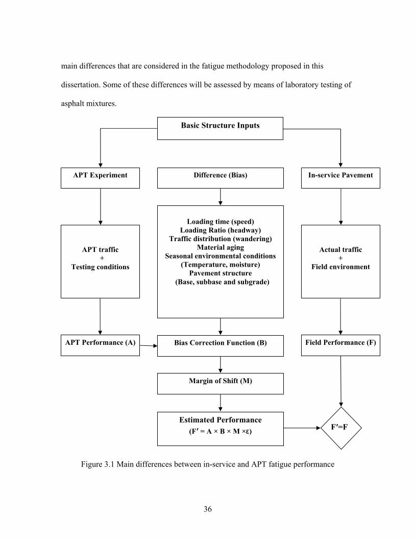
main differences that are considered in the fatigue methodology proposed in this
dissertation. Some of these differences will be assessed by means of laboratory testing of
asphalt mixtures.
APT Performance (A)
APT Experiment
APT traffic +
Testing conditions
Margin of Shift (M)
Bias Correction Function (B)
Loading time (speed)
Loading Ratio (headway) Traffic distribution (wandering)
Material aging Seasonal environmental conditions
(Temperature, moisture) Pavement structure
(Base, subbase and subgrade)
Difference (Bias)
Estimated Performance (F′ = A × B × M ×ε)
Basic Structure Inputs
Field Performance (F)
Actual traffic +
Field environment
F′=F
In-service Pavement
Figure 3.1 Main differences between in-service and APT fatigue performance
36
Due to the various conditions indicated in Figure 3.1, both sites perform differently.
APT performance (A) constitutes a biased estimate of in-service performance (F).
Therefore, a Bias Correction Factor (B) must be incorporated to account for these
differences. In addition, due to the high variability and uncertainties inherent to the
process and the effects of unobserved variables, the incorporation of a margin of shift
(M) is desirable to account for the unquantifiable differences. By incorporating these two
aspects into the formulation, the in-service performance can now be modified by
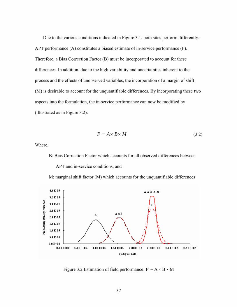
(illustrated as in Figure 3.2):
MBAF ××= (3.2)
Where,
B: Bias Correction Factor which accounts for all observed differences between
APT and in-service conditions, and
M: marginal shift factor (M) which accounts for the unquantifiable differences
Figure 3.2 Estimation of field performance: F′ = A × B × M
37
This equation provides a means to estimate the expected in-service fatigue
(or
for
n
It should be noted that the “shift factor” approach commonly used to correlate
.
ner,
tion
Equation 3.2 represents the expected value of F. No matter how accurately the bias
performance of a pavement site (F), when the expected performance of the same
similar) site has been previously determined through APT (A). The equation provides
the incorporation of a margin of shift factor to account for expected but unobserved
differences, field variability and other sources of uncertainty. All variables in Equatio
3.2 are random variables, which are characterized by a given distribution function.
laboratory and field performance is the simplest version of a Bias Correction Factor
While the shift factor is a deterministic number, usually determined in an ad-hoc man
the bias factor is statistically determined and characterized: it has a distribution. In
addition, by using a Bias Correction Function instead of a correction factor, an equa
can be developed that can incorporate variables affecting the value of the factor.
correction factor and the shift factor are estimated, due to unobserved variables and the
random nature of A, B, M and F, a random model error is actually present, therefore:
ε×××= MBAF (3.3)
Empirical evidence supports that performance functions such as F and A can be
assumed to follow a log-normal distribution. Thus, if the formulation of the bias
38

correction function, B, and the marginal shift factor, M, are such that they can be
assumed to be log-normal random variables, then the prediction error can be give
)log()log()log()log( MBAF
n by:
−×−=ε (3.4)
Under the above-mentioned assumptions, the predic
.4 is a log-normal random variable with mean equal to zero. It takes the form:
tion error defined by Equation
3
( )2,0)log( )log(εσε N≈ (3.5)
Where,
ε: unbiased random error term,
(ε): std. deviation of the prediction error.
imation of the fatigue life of in-service
ites based on the observed performance of similar sites under APT conditions will be
p
ed methodology for fatigue cracking prediction, four
ain steps are required. The first step consists of obtaining and analyzing cracking
’s
ts
σ log
The reliability-based methodology for the est
s
im lemented in four steps, which are discussed in the following section.
3.2 Methods and Procedures
To develop a reliability bas
m
performance data from sites tested under APT and similar in-service sites from FHWA
LTPP studies, the objective of which is to address the difference between APT resul
39

and in-service pavement fatigue performance. In the second step, Bias Correction
Functions will be developed to estimate Bias Correction Factors, the objective of which
to quantify the difference between APT and in service conditions. The third step is
develop the marginal shift factor and calibration, which will account for all
unquantifiable differences between the performance of the pavement site under APT and
in-service conditions. The final step consists of the reliability analysis, the o
which is to account for uncertainties and to obtain pavement performance estimations and
their respective variability.
The systematic compone
is
to
bjective of
nt of the unobserved differences and other differences of
condary order effect will be considered by the incorporation of a marginal shift factor
he
logy,
se of limited available data, and
he expected performance as well as an estimate of its
ty calculations.
se
(M). The random differences between observed and predicted behavior will be part of t
unbiased model error. As outlined in Figure 3.1, the shift factor approach, statistical and
mechanistic modeling are combined into one general approach that builds on their
individual strengths to overcome some of the shortcomings when the models are applied
individually (Prozzi et al., 2005). By combining the three models into one methodo
the utilization of the available data is optimized. In addition, this combined methodology
is preferred because:
1) It is scientifically sound,
2) It makes optimal u
3) It provides an estimate of t
variability. This becomes very important for reliabili
40

3.3 Reliability-based Fatigue Performance Prediction
In the past, prediction models developed from full scale or laboratory tests have been
used to predict performance. It is also known that a great spatial variability exists among
the
s,
ties in
e first time in
the 1993 AASHTO design method, which uses a reliability-based approach to account for
the
numerous pavement structural components, such as layer material properties and
layer thicknesses as a result of the construction of the pavement. There are also variations
in layer material quality, homogeneity, environmental conditions, and construction
techniques. Another source of spatial variability is due to the dynamic loads applied to
the pavement structure by the moving traffic. As a result of all these spatial variation
the distributions of stresses, strains, and deformations within the pavement structure are
by no means uniform and lead to the development of non uniform distribution of
distresses in the pavement. Before reliability concepts were employed in probabilistic
pavement design, shift factors were widely used to account for the many uncertain
the deterministic pavement design method. This generally resulted in over-design or
under-design, depending on the applied shift factors. The factors applied in the design
usually reflected the magnitude of the variation of all the design variables.
A more realistic procedure called probabilistic design was applied for th
uncertainties in the design variables and introduced desired level of reliability into the
pavement design. The AASHTO definition of reliability is: "The reliability of the
pavement design-performance process is the probability that a pavement site designed
41
using the process will perform satisfactorily over the traffic and environmental
conditions for the design period" (AASHTO, 1993). The limit state is assumed to be
reached when the predicted number of ESALs reaches the number that the site can
withstand before it reaches a specified terminal level of serviceability. In the AASHTO
Design Guide (1993), closed form solutions are used to develop designs for the chosen
reliability level.
Reliability based methodology for pavement performance (such as fatigue cracking)
prediction was recently proposed (Prozzi et al., 2005; Sun and Hudson, 2005) and is
furt
ach
n
ent
her developed in the early part of this research (Prozzi and Guo, 2007). Through this
approach, the three models suggested previously are combined into one general appro
that builds on their individual strengths to overcome some of the shortcomings when the
models are applied individually. The unobserved differences and other differences of
secondary order effect are considered part of the model error. In this dissertation, a
reliability based methodology for fatigue cracking prediction is developed. As shown i
Figure 3.3, let W(t) = A×B×M denote the allowable traffic loading repetitions (or
ESALs) predicted from APT and laboratory testing when the performance of pavement
structure deteriorates to a certain level and let W(T) be the actual in-service pavem
traffic loading repetitions, then the definition of reliability is expressed by Equation 3.6:
[ ] W(t) W(T)y Probabilit R <= (3
.6)
42
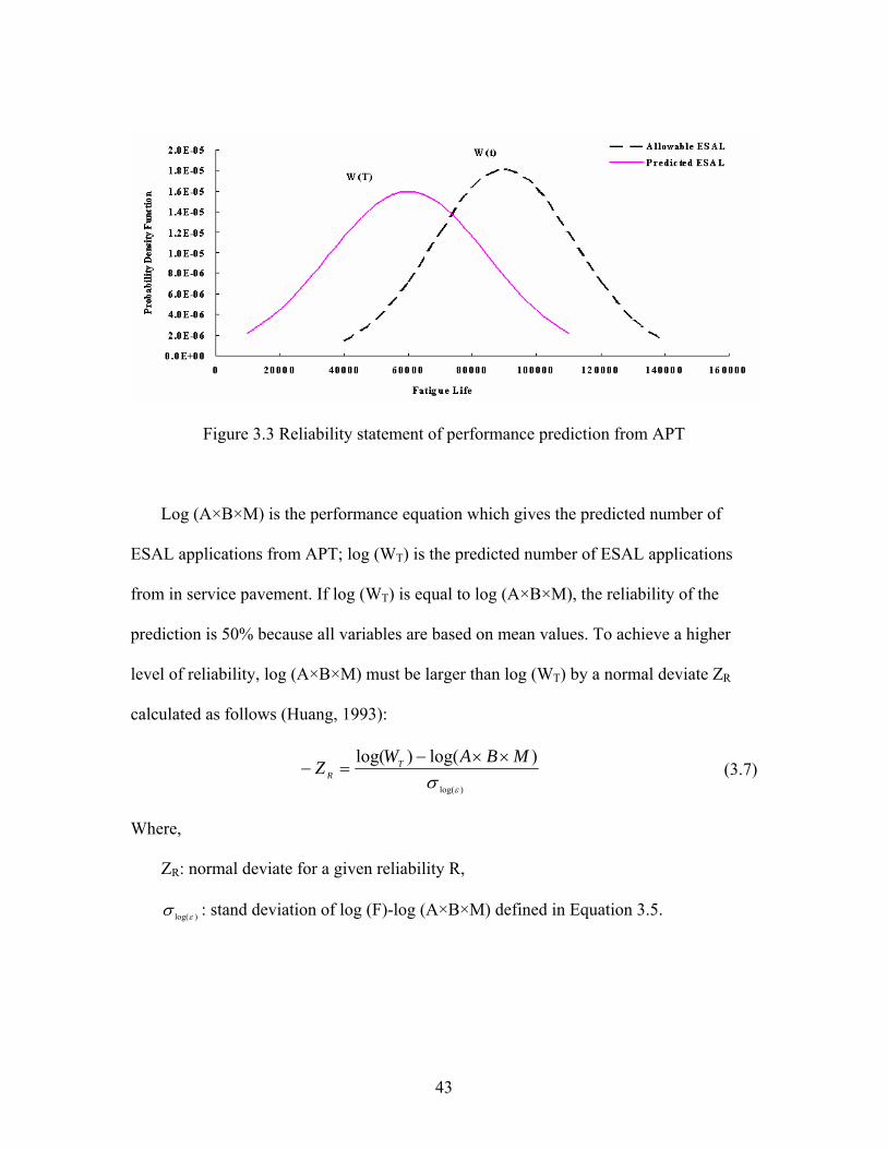
Figure 3.3 Reliability statement of performance prediction from APT
og (A×B×M) is the performance equation which gives the predicted number of
ESA
L
L applications from APT; log (WT) is the predicted number of ESAL applications
from in service pavement. If log (WT) is equal to log (A×B×M), the reliability of the
prediction is 50% because all variables are based on mean values. To achieve a higher
level of reliability, log (A×B×M) must be larger than log (WT) by a normal deviate ZR
calculated as follows (Huang, 1993):
)log(
)log()log(WZ =−εσ
MBATR
××− (3.7)
Where,
normal deviate for a given reliability R, ZR:
)log(εσ : stand deviation of log (F)-log (A×B×M) defined in Equation 3.5.
43
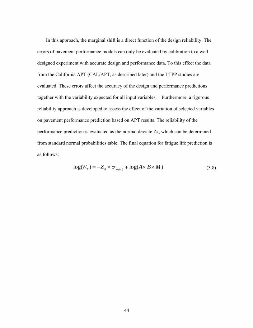
In this approach, the marginal shift is a direct function of the design reliability. The
errors of pavement performance models can only be evaluated by calibration to a well
designed experiment with accurate design and performance data. To this effect the data
from the California APT (CAL/APT, as described later) and the LTPP studies are
evaluated. These errors affect the accuracy of the design and performance predictions
together with the variability expected for all input variables. Furthermore, a rigorous
reliability approach is developed to assess the effect of the variation of selected variables
on pavement performance prediction based on APT results. The reliability of the
performance prediction is evaluated as the normal deviate ZR, which can be determined
from standard normal probabilities table. The final equation for fatigue life prediction is
as follows:
)log()log( )log( MBAZW RT ××+×−= εσ (3.8)
44

Chapter 4: Gathering and Processing of Performance Data
The first step in the reliability-based methodology consists of collecting cracking
performance data from sites tested under APT and similar in-service sites from FHWA’s
LTPP databases. Caltrans’ fleet of Heavy Vehicle Simulators (HVS) and FHWA’s
Accelerated Loading Facilities (ALF) represent the most successful APT programs
worldwide and have been collecting performance information on numerous mixes and
pavements for several years.
4.1 Caltrans Accelerated Pavement Testing Program (CAL/APT)
From 1994 to 1996, the University of California at Berkeley (UCB), in a joint effort
with the California Department of Transportation (Caltrans) and other agencies, utilized
two Heavy Vehicle Simulators (HVS) to study the accelerated loading on four full-scale
pavements with untreated aggregate and asphalt treated permeable bases (ATPB). One of
the HVS units was used to test in-service pavements while the other was utilized for
testing environment-controlled full-scale pavements at UCB’s Richmond Field Station
(RFS). The primary objective was to develop data to quantitatively verify existing
Caltrans design methodologies for different pavement types. A secondary objective was
to determine and compare fatigue lives of the different types of pavement structures. For
this research, test results from CAL/APT on pavement structure (Figure 4.1) containing
untreated aggregate base site 501RF and 503RF were collected (Harvey et al., 1999).
45
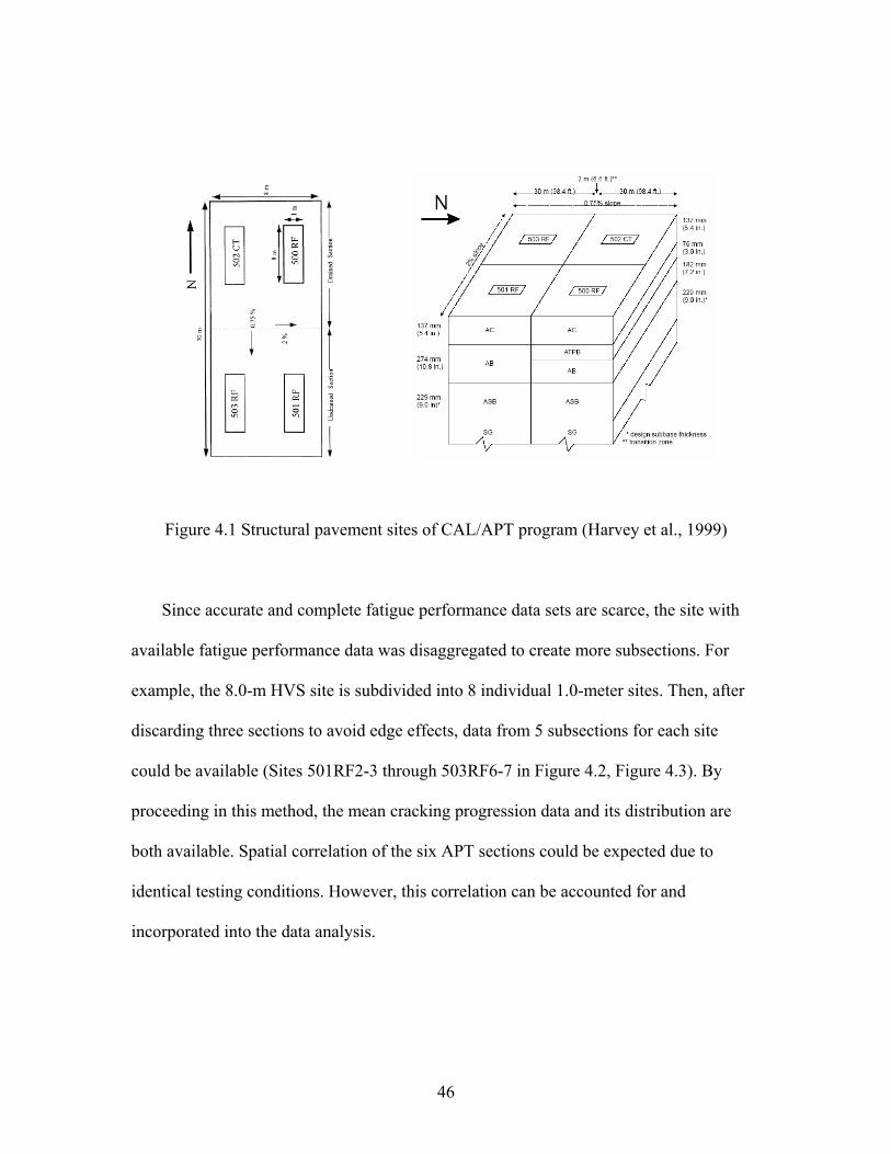
Figure 4.1 Structural pavement sites of CAL/APT program (Harvey et al., 1999)
Since accurate and complete fatigue performance data sets are scarce, the site with
available fatigue performance data was disaggregated to create more subsections. For
example, the 8.0-m HVS site is subdivided into 8 individual 1.0-meter sites. Then, after
discarding three sections to avoid edge effects, data from 5 subsections for each site
could be available (Sites 501RF2-3 through 503RF6-7 in Figure 4.2, Figure 4.3). By
proceeding in this method, the mean cracking progression data and its distribution are
both available. Spatial correlation of the six APT sections could be expected due to
identical testing conditions. However, this correlation can be accounted for and
incorporated into the data analysis.
46
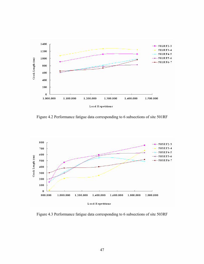
Figure 4.2 Performance fatigue data corresponding to 6 subsections of site 501RF
Figure 4.3 Performance fatigue data corresponding to 6 subsections of site 503RF
47
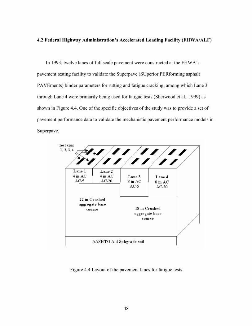
4.2 Federal Highway Administration’s Accelerated Loading Facility (FHWA/ALF)
In 1993, twelve lanes of full scale pavement were constructed at the FHWA’s
pavement testing facility to validate the Superpave (SUperior PERforming asphalt
PAVEments) binder parameters for rutting and fatigue cracking, among which Lane 3
through Lane 4 were primarily being used for fatigue tests (Sherwood et al., 1999) as
shown in Figure 4.4. One of the specific objectives of the study was to provide a set of
pavement performance data to validate the mechanistic pavement performance models in
Superpave.
Figure 4.4 Layout of the pavement lanes for fatigue tests
48

Figure 4.5 shows the cracking data of the nine fatigue test sites. Lane 1 site 2 and lane
2 site 2 are not included in the data analysis because both of these sites failed prematurely
under rutting. Lane 1 site 3 was also excluded because of poor drainage and early failure
due to a heavy rain storm.
Figure 4.5 Percentage of area cracked corresponding to nine fatigue test sites
4.3 In-service Pavement Performance Data (LTPP)
Initiated as part of SHRP, the LTPP program was established by the Transportation
Research Board (TRB) of the National Research Council in the early 1980’s and
sponsored by FHWA in cooperation with AASHTO. The motivation of the LTPP
program is to better understand pavement performance under the effects of various
variables. The overall objective of this program was to monitor and evaluate in-service
pavement performance under a variety of affecting factors over a pavement’s service life
49
for as long as 20 years (SHRP, 1994). Two main categories of pavement test sites are
included in the LTPP database, among which General Pavement Studies (GPS) are
existing pavements while Specific Pavement Studies (SPS) are sites where multiple test
sites of differing experimental treatment factors were specifically constructed (FHWA,
2003).
The LTPP pavement performance database is divided into several modules
containing multiple tables, among which the pavement monitoring (MON) module
contains manual distress and inventory (INV) module contains inventory information for
all GPS test sites. As one of the main LTPP products, the LTPP DataPave Online
provides a fast and easy means of navigating the complex structure of the LTPP relational
database.
According to the CAL/APT program, 3 similar in-service pavement sites with 5.8
inches (±5%) of asphalt concrete (AC) surface layer are selected from the LTPP database
(Table 4.1). According to the FHWA/ALF program, 4 similar in-service pavement sites
with 4 inches and 8 inches (±5%) of asphalt concrete (AC) surface layer are selected
from the LTPP database (Table 4.2).
50

Table 4.1 Selected LTPP sites match CAL/APT program
Table 4.2 Selected LTPP sites match FHWA/ALF program
51
The performance data from CAL/APT and FHWA/ALF provide the distribution of
A, while the data from LTPP provide the distribution of F (Figure 3.1). The link between
these two databases is established by means of Bias Correction Factor (variable B) and
the marginal shift factor M. Data for the determination of F is obtained from the fatigue
cracking tables contained in the LTPP pavement performance monitoring database.
Initially, data for the equivalent LTPP sites is typically obtained from the fatigue cracking
tables GATOR_CRACK_A contained in DataPave, which is expressed in squared meters
and the data contained in the tables corresponding to alligator cracking are used at the
various levels of severity (low, medium, high) (FHWA, 2006). Longitudinal cracking and
transverse cracking data are also used as that contained in tables TRANS_CRACK_ L (L,
M and H), TRANS_CRACK_ N (L, M and H), LONG_CRACK_WP_L (L, M and H)
and LONG_CRACK_NWP_L (L, M, H). These data are updated every year and are
available at http://www.ltpp-products.com. A most recent update can be obtained on
request from FHWA.
52
Chapter 5: Development of the Bias Correction Factor
In addition to pavement and material properties, the main factors that need to be
considered for developing an accurate methodology are traffic loading and
environment-related variables. To be specific, these factors are loading frequency
(speed), loading ratio (LR: rest periods over loading time), traffic distribution
(wandering), moisture, temperature and other long term effects such as climate and age
hardening of asphalt. The Bias Correction Factor should account for all quantifiable
differences of these factors between the performance of the pavement site under APT and
in-service conditions. In order to account for all differences, the Bias Correction Factor
can be represented as the product of a number of independent Bias Correction Functions
as in Equation 5.1:
K×××××= moistureetemperaturwanderioloadingratfrequency BCFBCFBCFBCFBCFB (5.1)
Where,
BCF frequency: Bias Correction Function to account for differences in loading speed,
BCF loading ratio: Bias Correction Function to account for differences in rest periods and
loading time,
BCF wander: Correction Function to account for differences in the lateral
distribution of traffic: channelized versus wandering,
BCF temperature: Bias Correction Function to account for differences in temperature,
and
53
BCF moisture: Bias Correction Function to account for differences in the moisture
content of the untreated granular materials.
All these correction functions are aimed at capturing the overall differential effect of
the specified variable between in-service pavements and similar pavements subjected to
APT, which is represented by the ratio of a given moment between the distribution of the
variables under in-service and APT, as in Equation 5.2, the parameter α reflects the
sensitivity of a particular process to a change in the level of variable x. This parameter
represents the order of the moment.
∫∫
∫∫
=
=
APTAPTAPT
ininingeneric
inin
APTAPTgeneric
dxxfxD
dxxfxDBCF
or
dxxfxg
dxxfxgBCF
in
APT
)()(
)()](
)()(
)()(
α
α
α
(5.2)
Where,
xin: variable of interest under in-service conditions,
xAPT: variable of interest under APT conditions, and
α: parameter that reflects the sensitivity of a particular process to a change in the
level of variable x. This parameter represents the order of the moment,
g(x): fatigue life as a function of variable x, and
D(x): damage as a function of variable x, and
f(x): density function of variable x.
54

When the variable of interest is not continuously distributed, the correction functions
are then represented as in Equation 5.3:
∑
∑= n
APTiAPTi
m
iin
generic
xpxg
xpxgBCF
iin
1
1.
)()(
)()(.
α
α
(5.3)
Where,
p(x.i): proportion of variable of interest in condition i,
m, n: number of conditions considered in the analysis (e.g. seasons).
During this research, BCFs are developed based on previous research results and
experience or computer simulations. In those cases where appropriate data are not
available for developing the specification form of the models or for testing the
recommended methodology and “fine-tuning” of the actual factors, laboratory testing is
carried out. This laboratory testing consists primarily of third-point bending tests and
dynamic stiffness. In the hypothetical case when the testing of the APT site is such that
all expected differences can be accounted for, then the value of the bias factor should be
unity. For example, if the wandering under APT is the same as the wandering observed
in-service, the Bias Correction Function for wandering will be one.
5.1 Bias Correction Function for Temperature and Loading Frequency (Speed)
55
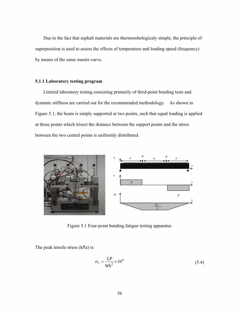
Due to the fact that asphalt materials are thermorehologicaly simple, the principle of
superposition is used to assess the effects of temperature and loading speed (frequency)
by means of the same master curve.
5.1.1 Laboratory testing program
Limited laboratory testing consisting primarily of third-point bending tests and
dynamic stiffness are carried out for the recommended methodology. As shown in
Figure 5.1, the beam is simply supported at two points, such that equal loading is applied
at those points which trisect the distance between the support points and the stress
between the two central points is uniformly distributed.
P
z
x
Pa aaP
v
xP
2Pa
−
x
M
Figure 5.1 Four-point bending fatigue testing apparatus
The peak tensile stress (kPa) is:
62
10×=WhLP
tσ (5.4)
56
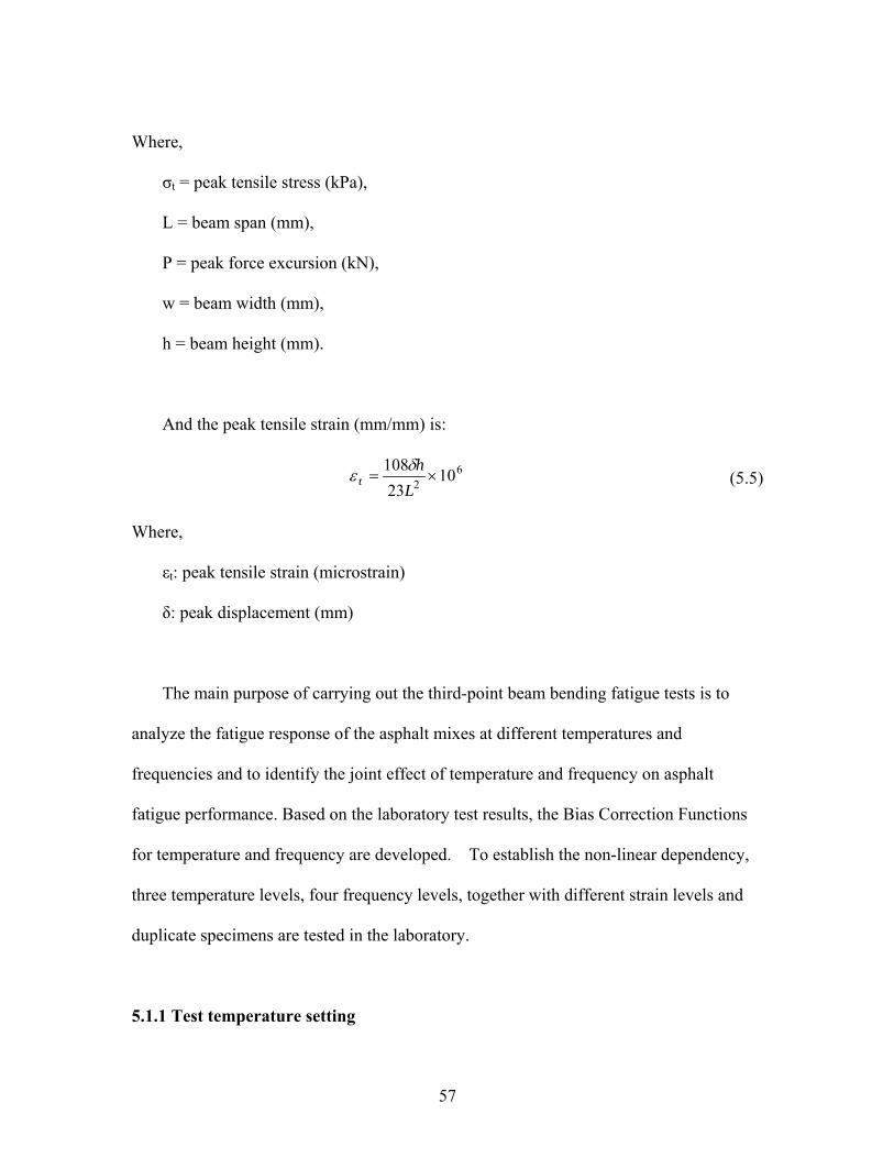
Where,
σt = peak tensile stress (kPa),
L = beam span (mm),
P = peak force excursion (kN),
w = beam width (mm),
h = beam height (mm).
And the peak tensile strain (mm/mm) is:
62 10
23108
×=L
ht
δε (5.5)
Where,
εt: peak tensile strain (microstrain)
δ: peak displacement (mm)
The main purpose of carrying out the third-point beam bending fatigue tests is to
analyze the fatigue response of the asphalt mixes at different temperatures and
frequencies and to identify the joint effect of temperature and frequency on asphalt
fatigue performance. Based on the laboratory test results, the Bias Correction Functions
for temperature and frequency are developed. To establish the non-linear dependency,
three temperature levels, four frequency levels, together with different strain levels and
duplicate specimens are tested in the laboratory.
5.1.1 Test temperature setting
57
Asphalt pavements are known to exhibit fatigue distress or deterioration of binder
stiffness under repeated traffic load in the intermediate temperature range from about
10°C to 30°C (Deacon et al., 1994; Stuart et al., 2002). Based on these findings, three test
temperatures were selected in this research: 30°C, 20°C and 10°C.
5.1.2 Test loading frequency setting
The change in material temperature has the same effect as changing the loading
speed. As shown in Figure 5.2, the loading frequency applied to the bottom of AC layer
is a function of the length of tire contact area (a), the thickness of AC layer (h), the
driving speed and the load spread angle (θ°). Suggested by Shell (1978), the loading time
of 0.02s is representative of the range of a vehicle speed of 48 to 64 km/h, which
corresponds to a loading frequency of 8 Hz according to Equation 5.6, which could also
be referred to calculate loading frequencies at different speed (Table 5.1).
Figure 5.2 Mode for loading speed (frequency) calculation
58
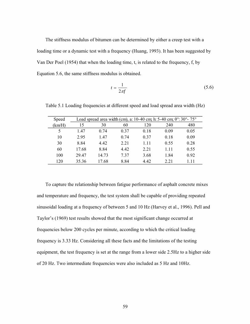
The stiffness modulus of bitumen can be determined by either a creep test with a
loading time or a dynamic test with a frequency (Huang, 1993). It has been suggested by
Van Der Poel (1954) that when the loading time, t, is related to the frequency, f, by
Equation 5.6, the same stiffness modulus is obtained.
ft
π21
= (5.6)
Table 5.1 Loading frequencies at different speed and load spread area width (Hz)
15 30 60 120 240 4805 1.47 0.74 0.37 0.18 0.09 0.0510 2.95 1.47 0.74 0.37 0.18 0.0930 8.84 4.42 2.21 1.11 0.55 0.2860 17.68 8.84 4.42 2.21 1.11 0.55100 29.47 14.73 7.37 3.68 1.84 0.92120 35.36 17.68 8.84 4.42 2.21 1.11
Speed(km/H)
Load spread area width (cm), a: 10-40 cm; h: 5-40 cm; θ°: 30°- 75°
To capture the relationship between fatigue performance of asphalt concrete mixes
and temperature and frequency, the test system shall be capable of providing repeated
sinusoidal loading at a frequency of between 5 and 10 Hz (Harvey et al., 1996). Pell and
Taylor’s (1969) test results showed that the most significant change occurred at
frequencies below 200 cycles per minute, according to which the critical loading
frequency is 3.33 Hz. Considering all these facts and the limitations of the testing
equipment, the test frequency is set at the range from a lower side 2.5Hz to a higher side
of 20 Hz. Two intermediate frequencies were also included as 5 Hz and 10Hz.
59
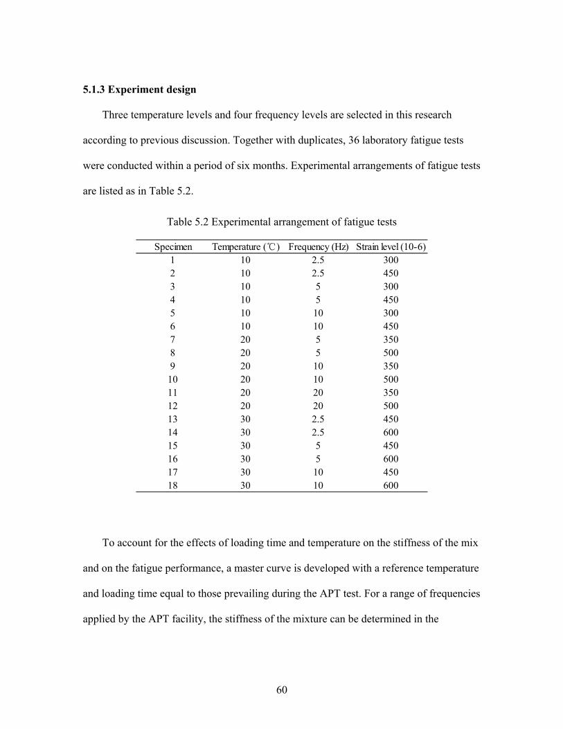
5.1.3 Experiment design
Three temperature levels and four frequency levels are selected in this research
according to previous discussion. Together with duplicates, 36 laboratory fatigue tests
were conducted within a period of six months. Experimental arrangements of fatigue tests
are listed as in Table 5.2.
Table 5.2 Experimental arrangement of fatigue tests
Specimen Temperature (℃) Frequency (Hz) Strain level (10-6)1 10 2.5 3002 10 2.5 4503 10 5 3004 10 5 4505 10 10 3006 10 10 4507 20 5 3508 20 5 5009 20 10 350
10 20 10 50011 20 20 35012 20 20 50013 30 2.5 45014 30 2.5 60015 30 5 45016 30 5 60017 30 10 45018 30 10 600
To account for the effects of loading time and temperature on the stiffness of the mix
and on the fatigue performance, a master curve is developed with a reference temperature
and loading time equal to those prevailing during the APT test. For a range of frequencies
applied by the APT facility, the stiffness of the mixture can be determined in the
60

laboratory at different temperatures. Then, the data obtained at different temperatures is
shifted horizontally so as to build the master curve, which is shown in Figure 5.3. The
amount of shifting that takes place at each temperature reflects the frequency and
temperature dependency of the material.
Figure 5.3 Master curve of a particular asphalt mixture
The master curve is typically developed from dynamic modulus testing of the
material by means of tri-axial testing. For the purpose of this research, however, it is
proposed to base the master curve on stiffness determinations performed by means of
third-point bending test. The reasoning f this selection is that dynamic stiffness is closely
related to fatigue performance as opposed to dynamic modulus. It has been shown that
modified and unmodified asphalt mixtures with equivalent dynamic modulus may show
significantly different fatigue performance.
61
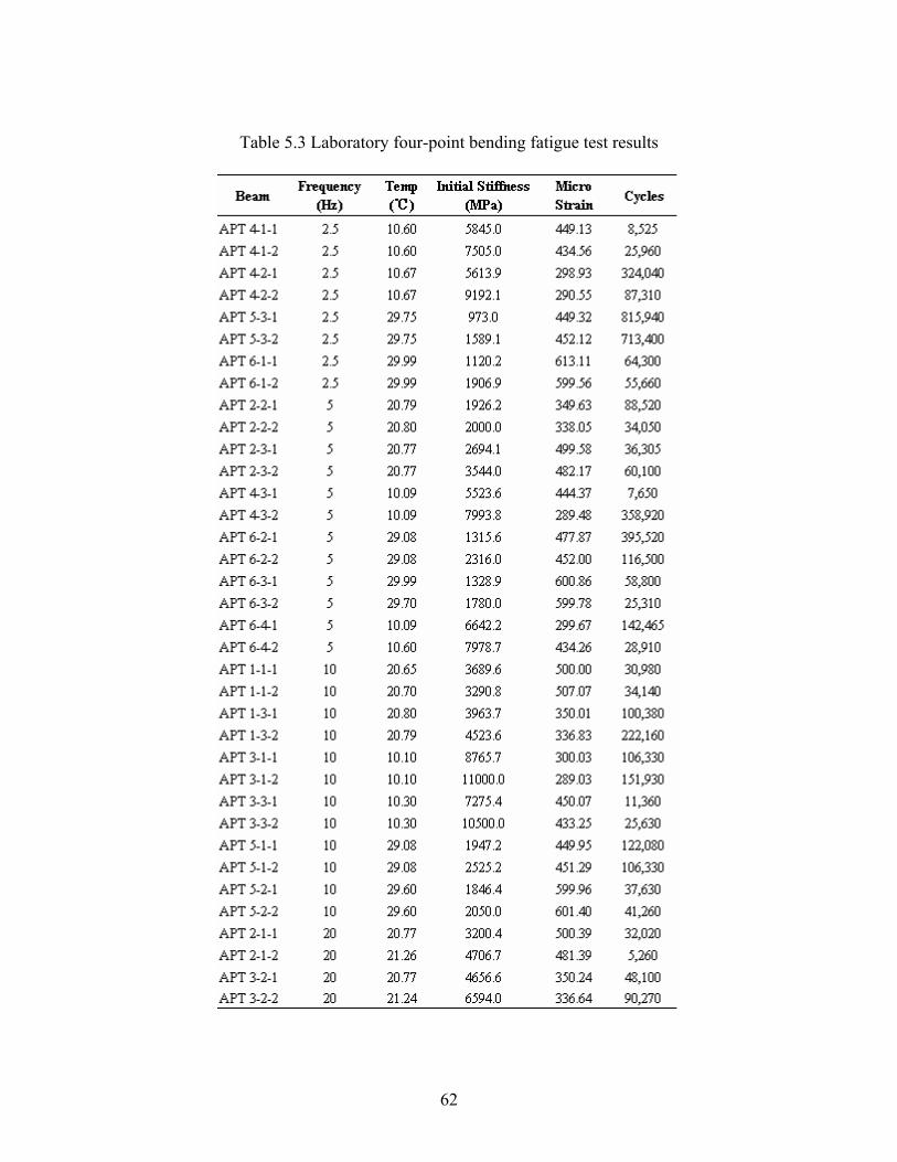
Table 5.3 Laboratory four-point bending fatigue test results
62
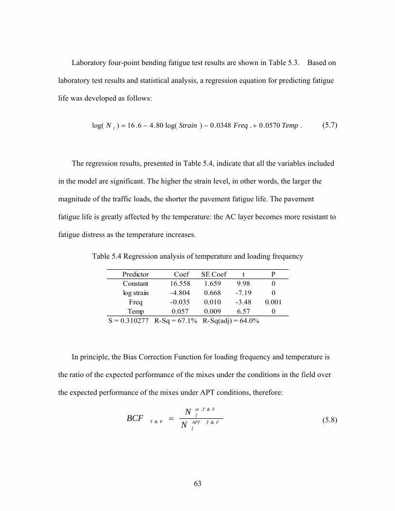
Laboratory four-point bending fatigue test results are shown in Table 5.3. Based on
laboratory test results and statistical analysis, a regression equation for predicting fatigue
life was developed as follows:
.0570.0.0348.0)log(80.46.16)log( TempFreqStrainN f +−−= (5.7)
The regression results, presented in Table 5.4, indicate that all the variables included
in the model are significant. The higher the strain level, in other words, the larger the
magnitude of the traffic loads, the shorter the pavement fatigue life. The pavement
fatigue life is greatly affected by the temperature: the AC layer becomes more resistant to
fatigue distress as the temperature increases.
Table 5.4 Regression analysis of temperature and loading frequency
Predictor Coef SE Coef t PConstant 16.558 1.659 9.98 0log strain -4.804 0.668 -7.19 0
Freq -0.035 0.010 -3.48 0.001Temp 0.057 0.009 6.57 0
S = 0.310277 R-Sq = 67.1% R-Sq(adj) = 64.0%
In principle, the Bias Correction Function for loading frequency and temperature is
the ratio of the expected performance of the mixes under the conditions in the field over
the expected performance of the mixes under APT conditions, therefore:
FTAPTf
FTinf
FT NN
BCF &,
&,
& = (5.8)
63

By replacing Equation 5.6 into Equation 5.7, thus, Bias Correction Function for
fatigue life as a function of loading frequency (Hz) and temperature (°C) can be
computed as:
)(0348.0)(0570.0& 10 APTFreqinFreqAPTTinT
FTBCF −−−= (5.9)
Where,
TAPT: pavement temperature during APT testing (°C),
Tin: pavement temperature in the field (°C),
FAPT: loading frequency during APT testing (Hz), and
Fin: loading frequency of in service pavement (Hz).
5.2 Bias Correction Function for Traffic Wandering
Unlike APT traffic, which is tightly controlled, actual highway traffic on in-service
pavements follows a random lateral distribution. Previous research has indicated that the
distribution could be characterized as normal with mean and standard deviation of the
lateral position being a function of the facility type, number of lanes and lane width
(Wang et al., 2000). Independent of the actual distribution, the traffic distribution will
produce a distribution of the maximum strain that develops in the asphalt concrete layer.
By denoting εx the random variable that represents the value of the maximum tensile
strain as a result of the horizontal traffic distribution and f(x) the probability density
function of this random variable, the Bias Correction Factor for traffic wandering
(BCFwander) can be calculated as follows:
64

∫∫=
−
−
ininin
APTAPTAPTWander dxxf
dxxfBCF)()()()(
β
β
εε
(5.10)
Where,
εin, εAPT: maximum tensile strain as a function of the lateral position x,
β: parameter that represents the sensitivity of the pavement fatigue life to a change in
strain, -4.8 based on laboratory test results,
f(x): probability density function of traffic distributed at lateral position x.
If APT is strictly controlled, which means there is no wandering for APT, this
equation can be simplified as Equation 5.11:
∫=
−
−
inininWander dxxf
BCF)()(
maxβ
β
εε
(5.11)
According to truck testing at the Virginia Smart Road, the maximum response as a
function of the lateral position could be fitted to an exponential curve (Al-Qadi and
Nassar, 2003):
)7199.1exp(931.0max xin −××= εε (5.12)
It is assumed that traffic is normally distributed along the lateral position x with a
mean of zero, the probability density function becomes:
)21exp(
21)(
2
⎥⎦⎤
⎢⎣⎡−=σπσxxf (5.13)
65
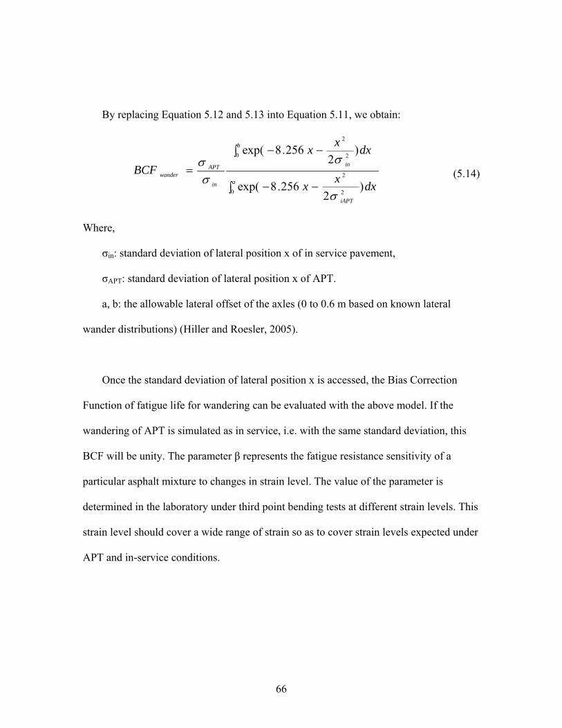
By replacing Equation 5.12 and 5.13 into Equation 5.11, we obtain:
∫ −−
∫ −−
=a
iAPT
b
in
in
APTwander
dxxx
dxxx
BCF0 2
2
0 2
2
)2
256.8exp(
)2
256.8exp(
σ
σ
σσ
(5.14)
Where,
σin: standard deviation of lateral position x of in service pavement,
σAPT: standard deviation of lateral position x of APT.
a, b: the allowable lateral offset of the axles (0 to 0.6 m based on known lateral
wander distributions) (Hiller and Roesler, 2005).
Once the standard deviation of lateral position x is accessed, the Bias Correction
Function of fatigue life for wandering can be evaluated with the above model. If the
wandering of APT is simulated as in service, i.e. with the same standard deviation, this
BCF will be unity. The parameter β represents the fatigue resistance sensitivity of a
particular asphalt mixture to changes in strain level. The value of the parameter is
determined in the laboratory under third point bending tests at different strain levels. This
strain level should cover a wide range of strain so as to cover strain levels expected under
APT and in-service conditions.
66

5.3 Bias Correction Function for Moisture
Moisture condition of pavement subgrade under APT is well controlled while
in-service subgrade is subjected to seasonal changes. This change relates primarily to the
variation of the bottom tensile strains of asphalt concrete layer and, therefore, to the
fatigue performance. With the multi-layer linear elastic assumption, the Bias Correction
Factor for moisture (BCFmositure) is determined with Equation 5.15:
∑=
=
n
Iiiniin
APTmoisture
pBCF
1.
8.4,
8.4
)(εε
ε (5.15)
Where,
εAPT: maximum tensile strain in the asphalt layer under APT,
εi: maximum seasonal tensile strain in the asphalt layer as a result of differential
support due to moisture changes,
p(εi): proportion of time in condition i,
n: number of seasons (typically 4 to 12 seasons are sufficient),
5.4 Bias Correction Function for Loading Ratio
The rest times in an APT experiment are shorter than those occurring on actual
highways but the loading time is longer because of the lower speeds typical of APT. This
can be illustrated by a loading ratio, which is defined as the ratio of rest period over
loading time (Figure 5.4). This translates into an increased amount of dissipated energy
67
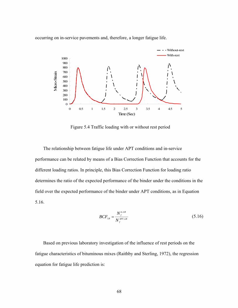
occurring on in-service pavements and, therefore, a longer fatigue life.
0100200300400500600700800900
1000
0 0.5 1 1.5 2 2.5 3 3.5 4 4.5 5
Time (Sec)
Mic
ro-S
train
Without-restWith-rest
Figure 5.4 Traffic loading with or without rest period
The relationship between fatigue life under APT conditions and in-service
performance can be related by means of a Bias Correction Function that accounts for the
different loading ratios. In principle, this Bias Correction Function for loading ratio
determines the ratio of the expected performance of the binder under the conditions in the
field over the expected performance of the binder under APT conditions, as in Equation
5.16.
LRAPTf
LRinf
LR NN
BCF,
,
= (5.16)
Based on previous laboratory investigation of the influence of rest periods on the
fatigue characteristics of bituminous mixes (Raithby and Sterling, 1972), the regression
equation for fatigue life prediction is:
68
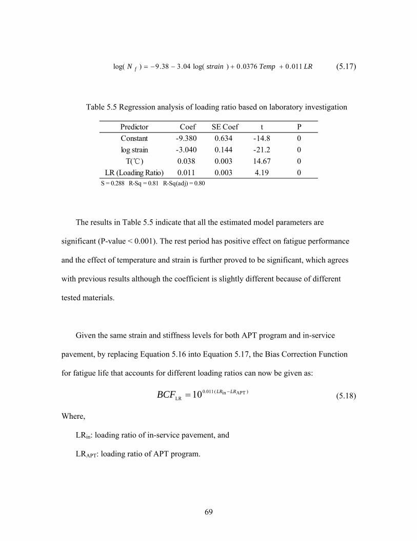
LRTempstrainN f 011.00376.0)log(04.338.9)log( ++−−= (5.17)
Table 5.5 Regression analysis of loading ratio based on laboratory investigation
Predictor Coef SE Coef t PConstant -9.380 0.634 -14.8 0log strain -3.040 0.144 -21.2 0
T(℃) 0.038 0.003 14.67 0LR (Loading Ratio) 0.011 0.003 4.19 0
S = 0.288 R-Sq = 0.81 R-Sq(adj) = 0.80
The results in Table 5.5 indicate that all the estimated model parameters are
significant (P-value < 0.001). The rest period has positive effect on fatigue performance
and the effect of temperature and strain is further proved to be significant, which agrees
with previous results although the coefficient is slightly different because of different
tested materials.
Given the same strain and stiffness levels for both APT program and in-service
pavement, by replacing Equation 5.16 into Equation 5.17, the Bias Correction Function
for fatigue life that accounts for different loading ratios can now be given as:
)APTin( 0.011LR 10 LRLRBCF −= (5.18)
Where,
LRin: loading ratio of in-service pavement, and
LRAPT: loading ratio of APT program.
69
Furthermore, according to Bonnaure’s results, the beneficial effect of rest periods on
fatigue life seems to reach a maximum when the loading ratio is up to 25 (Bonnaure et
al., 1982). LR will then take a value of 25 when the ratio is larger than 25.
5.5 Sensitivity Analysis of Bias Correction Functions
Sensitivity analysis is the determination of how variations in input parameters
quantitatively affect predicted distress. The goals of a sensitivity analysis are as follows:
(1) determination of the degree to which the distress prediction model can simulate
observed trends in the development and progression of distress; (2) determination of what
factors contribute to variability in the predicted distress; and (3) assessment of the
reasonability of the influence of the model parameters on the variability of the predicted
distress. With the use of Bias Correction Functions, sensitivity analyses were made to
determine the effects of loading frequency (speed), loading ratio, traffic distribution
(wandering), moisture, and temperature on pavement fatigue life prediction.
The Bias Correction Factor can now be represented as the product of a number of
independent Bias Correction Functions as in Equation 5.19, which was used to determine
the effect of various parameters on the Bias Correction Factor.
70
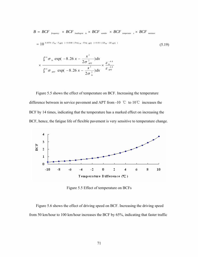
8.4
8.4
6.00 2
2
6.00 2
2
)APTin(011.0)(0348.0)(0570.0
)2
26.8exp(
)2
26.8exp(
10
−
−
−+−−−
×∫ −−
∫ −−
×
=
××××=
APT
in
inAPT
APTin
LRLRAPTFreqinFreqAPTTinT
moistureetemperaturwanderioloadingratfrequency
dxxx
dxxx
BCFBCFBCFBCFBCFB
εε
σσ
σσ
(5.19)
Figure 5.5 shows the effect of temperature on BCF. Increasing the temperature
difference between in service pavement and APT from -10 ℃ to 10℃ increases the
BCF by 14 times, indicating that the temperature has a marked effect on increasing the
BCF, hence, the fatigue life of flexible pavement is very sensitive to temperature change.
Figure 5.5 Effect of temperature on BCFs
Figure 5.6 shows the effect of driving speed on BCF. Increasing the driving speed
from 50 km/hour to 100 km/hour increases the BCF by 65%, indicating that faster traffic
71
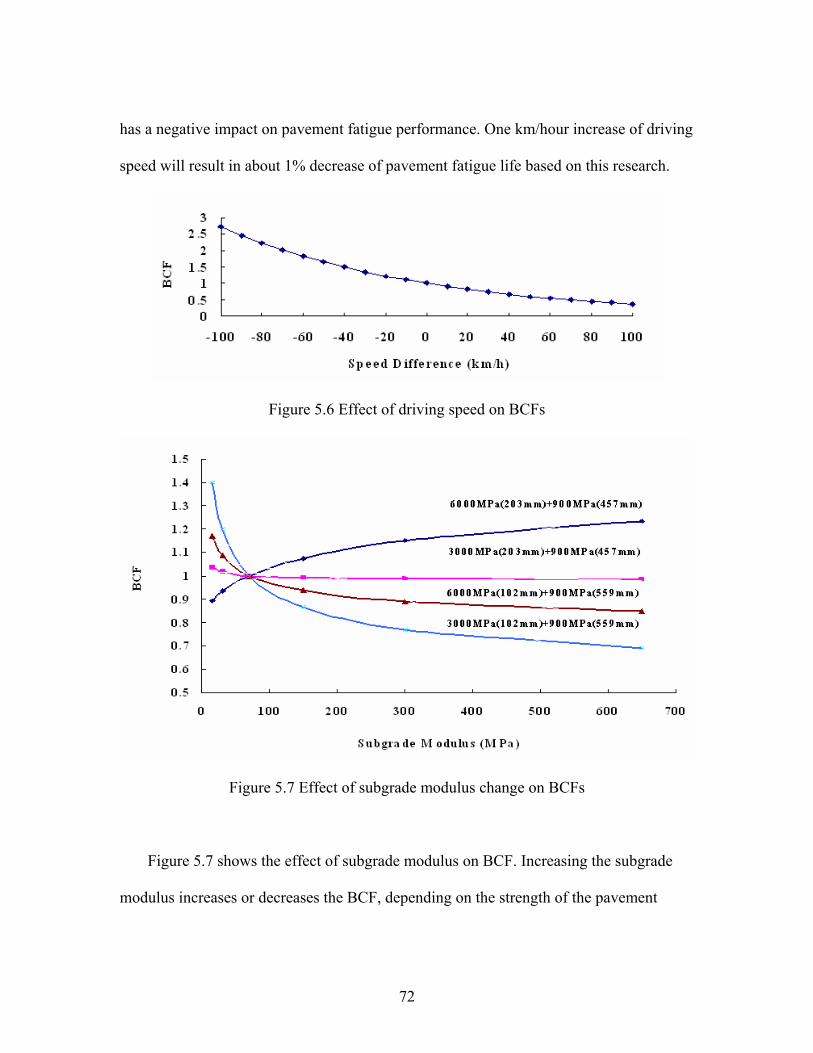
has a negative impact on pavement fatigue performance. One km/hour increase of driving
speed will result in about 1% decrease of pavement fatigue life based on this research.
Figure 5.6 Effect of driving speed on BCFs
Figure 5.7 Effect of subgrade modulus change on BCFs
Figure 5.7 shows the effect of subgrade modulus on BCF. Increasing the subgrade
modulus increases or decreases the BCF, depending on the strength of the pavement
72
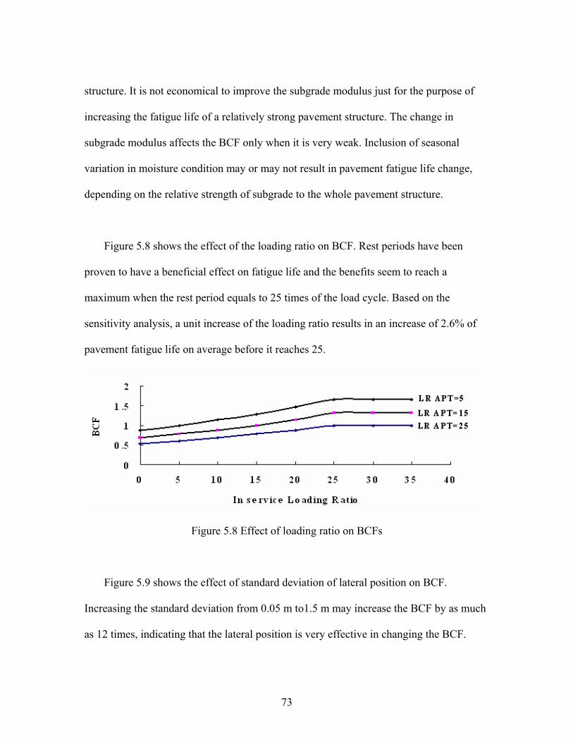
structure. It is not economical to improve the subgrade modulus just for the purpose of
increasing the fatigue life of a relatively strong pavement structure. The change in
subgrade modulus affects the BCF only when it is very weak. Inclusion of seasonal
variation in moisture condition may or may not result in pavement fatigue life change,
depending on the relative strength of subgrade to the whole pavement structure.
Figure 5.8 shows the effect of the loading ratio on BCF. Rest periods have been
proven to have a beneficial effect on fatigue life and the benefits seem to reach a
maximum when the rest period equals to 25 times of the load cycle. Based on the
sensitivity analysis, a unit increase of the loading ratio results in an increase of 2.6% of
pavement fatigue life on average before it reaches 25.
Figure 5.8 Effect of loading ratio on BCFs
Figure 5.9 shows the effect of standard deviation of lateral position on BCF.
Increasing the standard deviation from 0.05 m to1.5 m may increase the BCF by as much
as 12 times, indicating that the lateral position is very effective in changing the BCF.
73
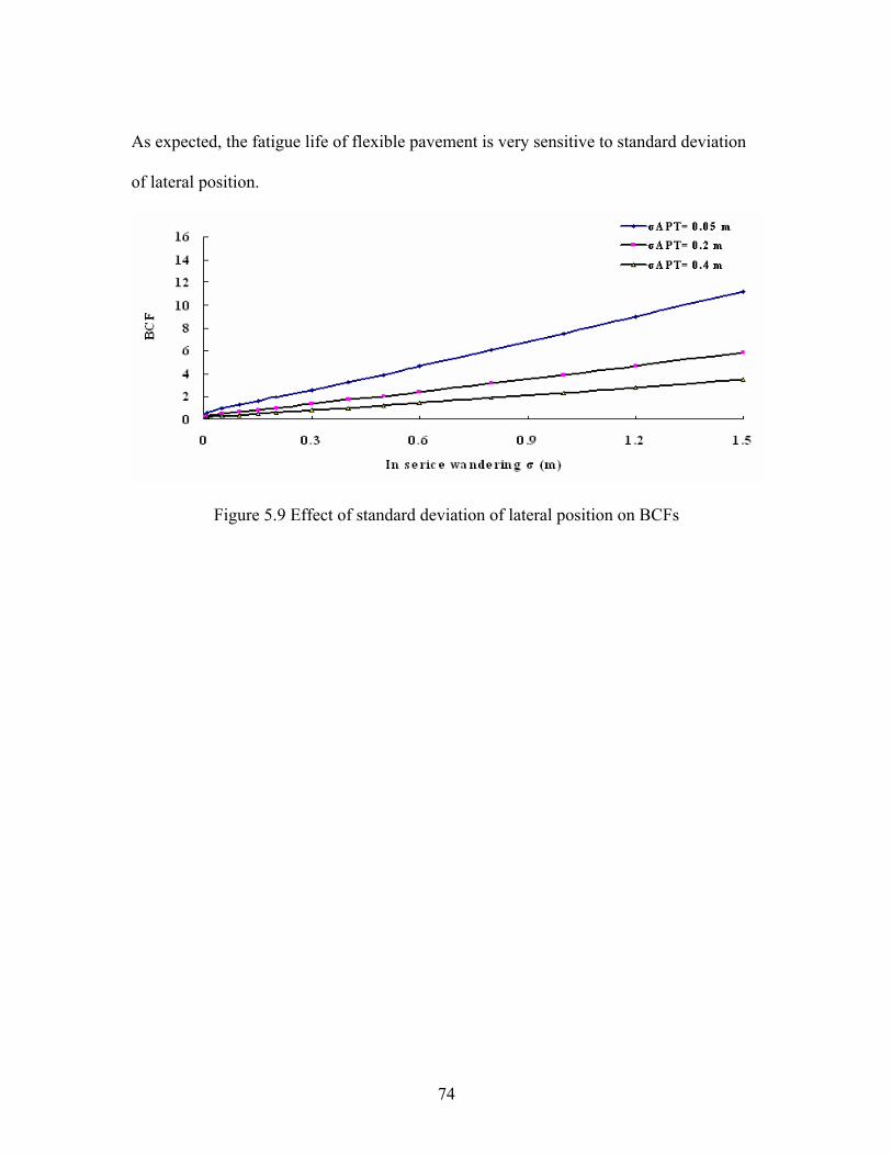
As expected, the fatigue life of flexible pavement is very sensitive to standard deviation
of lateral position.
Figure 5.9 Effect of standard deviation of lateral position on BCFs
74
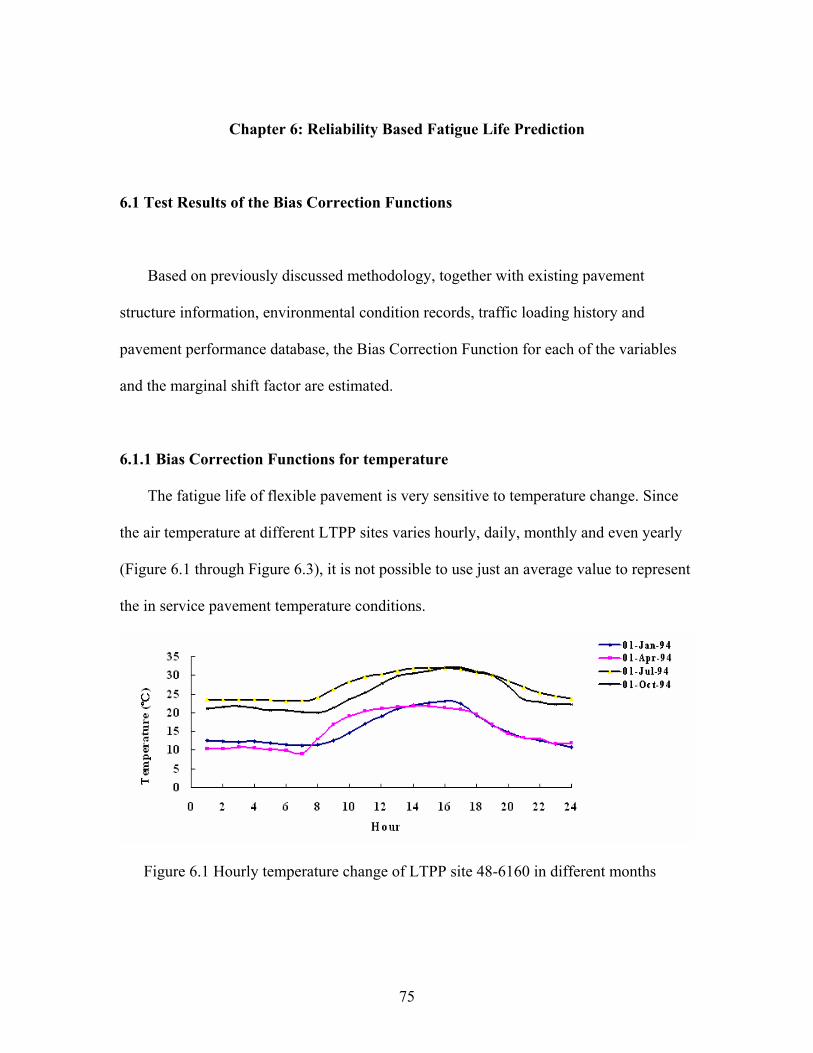
Chapter 6: Reliability Based Fatigue Life Prediction
6.1 Test Results of the Bias Correction Functions
Based on previously discussed methodology, together with existing pavement
structure information, environmental condition records, traffic loading history and
pavement performance database, the Bias Correction Function for each of the variables
and the marginal shift factor are estimated.
6.1.1 Bias Correction Functions for temperature
The fatigue life of flexible pavement is very sensitive to temperature change. Since
the air temperature at different LTPP sites varies hourly, daily, monthly and even yearly
(Figure 6.1 through Figure 6.3), it is not possible to use just an average value to represent
the in service pavement temperature conditions.
Figure 6.1 Hourly temperature change of LTPP site 48-6160 in different months
75
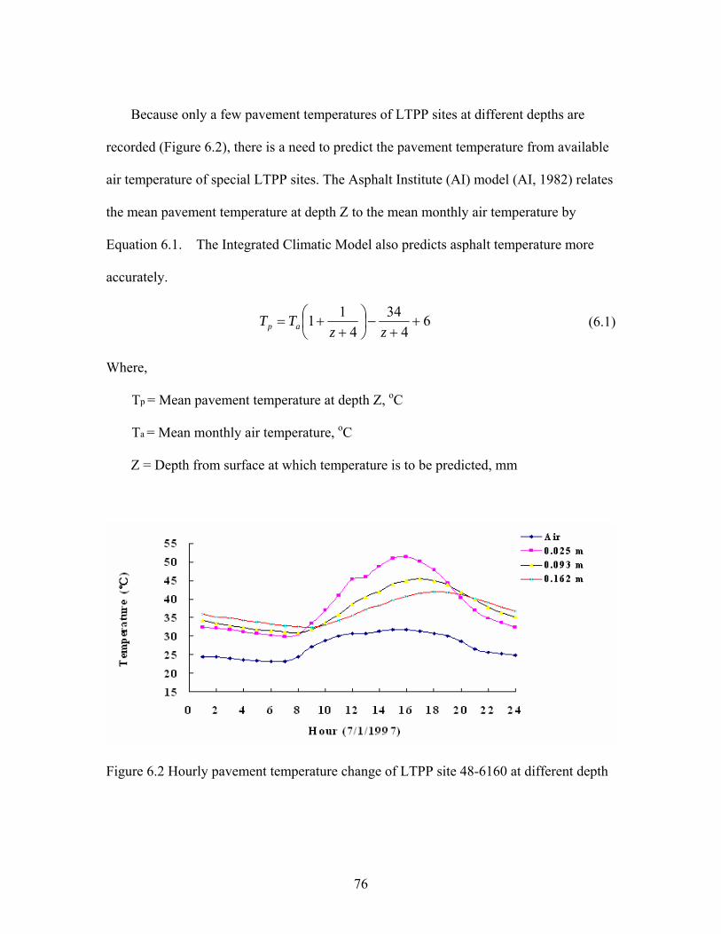
Because only a few pavement temperatures of LTPP sites at different depths are
recorded (Figure 6.2), there is a need to predict the pavement temperature from available
air temperature of special LTPP sites. The Asphalt Institute (AI) model (AI, 1982) relates
the mean pavement temperature at depth Z to the mean monthly air temperature by
Equation 6.1. The Integrated Climatic Model also predicts asphalt temperature more
accurately.
64
344
11 ++
−⎟⎠⎞
⎜⎝⎛
++=
zzTT ap (6.1)
Where,
Tp = Mean pavement temperature at depth Z, oC
Ta = Mean monthly air temperature, oC
Z = Depth from surface at which temperature is to be predicted, mm
Figure 6.2 Hourly pavement temperature change of LTPP site 48-6160 at different depth
76
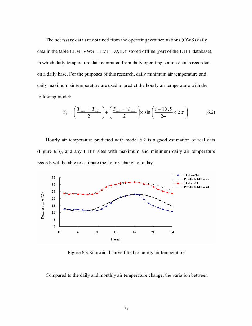
The necessary data are obtained from the operating weather stations (OWS) daily
data in the table CLM_VWS_TEMP_DAILY stored offline (part of the LTPP database),
in which daily temperature data computed from daily operating station data is recorded
on a daily base. For the purposes of this research, daily minimum air temperature and
daily maximum air temperature are used to predict the hourly air temperature with the
following model:
⎟⎠⎞
⎜⎝⎛ ×
−×⎟
⎠⎞
⎜⎝⎛ −
+⎟⎠⎞
⎜⎝⎛ +
= π224
5.10sin22
minmaxminmax iTTTTTi (6.2)
Hourly air temperature predicted with model 6.2 is a good estimation of real data
(Figure 6.3), and any LTPP sites with maximum and minimum daily air temperature
records will be able to estimate the hourly change of a day.
Figure 6.3 Sinusoidal curve fitted to hourly air temperature
Compared to the daily and monthly air temperature change, the variation between
77
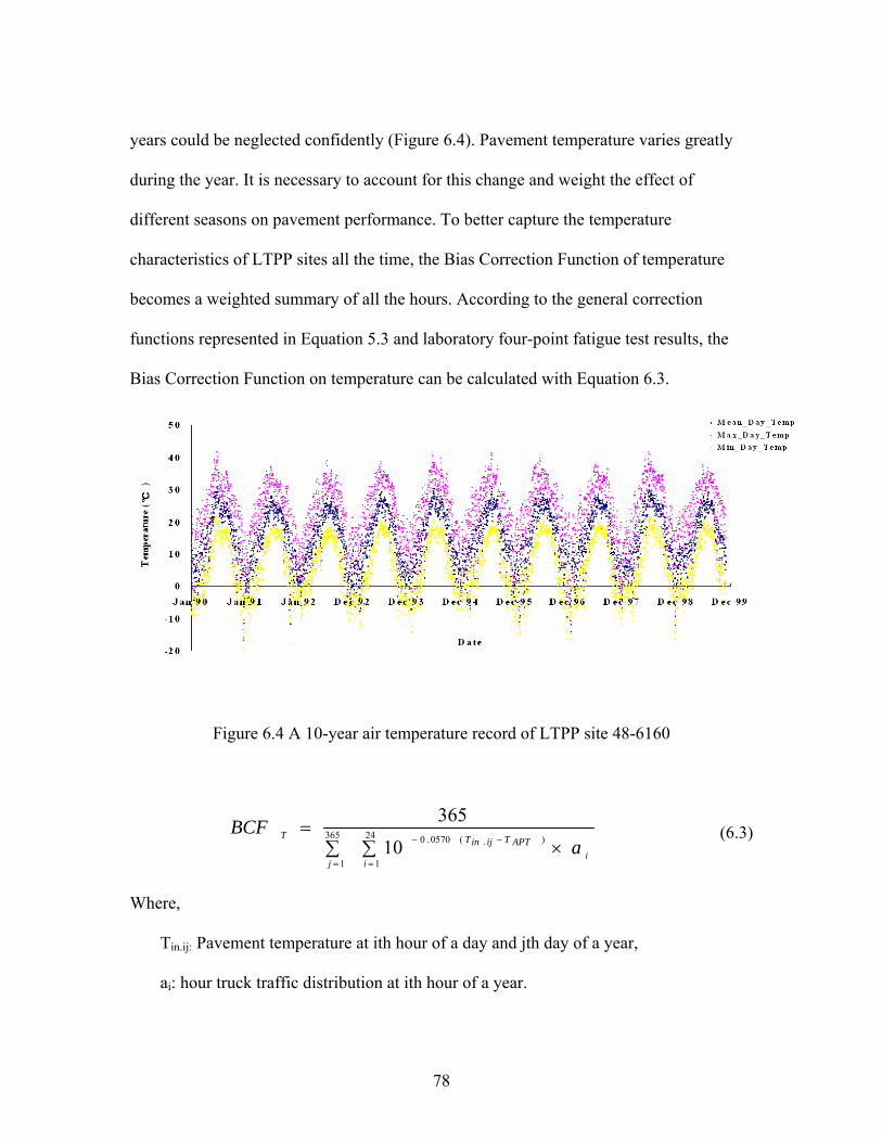
years could be neglected confidently (Figure 6.4). Pavement temperature varies greatly
during the year. It is necessary to account for this change and weight the effect of
different seasons on pavement performance. To better capture the temperature
characteristics of LTPP sites all the time, the Bias Correction Function of temperature
becomes a weighted summary of all the hours. According to the general correction
functions represented in Equation 5.3 and laboratory four-point fatigue test results, the
Bias Correction Function on temperature can be calculated with Equation 6.3.
Figure 6.4 A 10-year air temperature record of LTPP site 48-6160
∑ ×∑=
=
−−
=
24
1
).(0570.0365
110
365
ii
APTTijinT
j
Ta
BCF (6.3)
Where,
Tin.ij: Pavement temperature at ith hour of a day and jth day of a year,
ai: hour truck traffic distribution at ith hour of a year.
78

Table 6.1 is a summary Bias Correction Functions table of all the selected LTPP sites
to different APT temperatures.
Table 6.1 BCF of LTPP sites to different APT temperatures
6.1.2 Bias Correction Functions for frequency
At the seven LTPP sites selected, free flow conditions can be assumed; therefore,
traveling speeds were assumed to be close to the speed limit of each site (rural interstate).
Thus, the traffic loading frequency of in-service pavement (Fin) is assumed to be constant
in this research. In areas subjected to traffic congestion, the change of loading frequency
should be considered. Based on the speed limit information of each LTPP site, the
loading time (loading frequency) is calculated with Equation 5.6. With loading frequency
known, the Bias Correction Function can then be evaluated with Equation 5.9. Table 6.2
is a list of Bias Correction Functions on loading frequency for all seven LTPP sites.
6.1.3 Bias Correction Function for traffic wandering
Since the lateral wandering of APT sections was programmed to simulate the traffic
wandering on a typical highway lane, the Bias Correction Function for traffic wandering
should be set as one in this research.
79
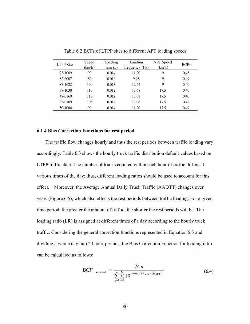
Table 6.2 BCFs of LTPP sites to different APT loading speeds
LTPP Sites Speed(km/h)
Loadingtime (s)
Loadingfrequency (Hz)
APT Speed(km/h)
BCFs
23-1009 90 0.014 11.20 9 0.4582-6007 80 0.016 9.95 9 0.4987-1622 100 0.013 12.44 9 0.4037-1030 110 0.012 13.68 17.5 0.4048-6160 110 0.012 13.68 17.5 0.4035-0109 105 0.012 13.06 17.5 0.4250-1004 90 0.014 11.20 17.5 0.49
6.1.4 Bias Correction Functions for rest period
The traffic flow changes hourly and thus the rest periods between traffic loading vary
accordingly. Table 6.3 shows the hourly truck traffic distribution default values based on
LTPP traffic data. The number of trucks counted within each hour of traffic differs at
various times of the day; thus, different loading ratios should be used to account for this
effect. Moreover, the Average Annual Daily Truck Traffic (AADTT) changes over
years (Figure 6.5), which also effects the rest periods between traffic loading. For a given
time period, the greater the amount of traffic, the shorter the rest periods will be. The
loading ratio (LR) is assigned at different times of a day according to the hourly truck
traffic. Considering the general correction functions represented in Equation 5.3 and
dividing a whole day into 24 hour-periods, the Bias Correction Function for loading ratio
can be calculated as follows:
∑ ∑=
= =
−n
j i
LRLR
nBCF
1
24
1
)APTin.ij( 0.011-periodrest 10
24 (6.4)
80
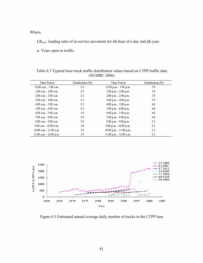
Where,
LRin.ij: loading ratio of in-service pavement for ith hour of a day and jth year.
n: Years open to traffic.
Table 6.3 Typical hour truck traffic distribution values based on LTPP traffic data (NCHRP, 2006)
Figure 6.5 Estimated annual average daily number of trucks in the LTPP lane
81

The minimum rest period is calculated with the maximum AADTT and the busiest
hour of a day. In this research, the loading ratios of the seven selected LTPP sites and
APT programs are all above 25 and thus a value of 25 is used, as shown in Table 6.4.
Table 6.4 BCFs of LTPP sites to different APT loading ratio
6.1.5 Bias Correction Functions for moisture
The KENLAYER computer program (Huang, 2004) is used to calculate the tensile
strain at the bottom of the asphalt layer under the application of a 40 kN dual-tire load
having 690 kPa tire pressure and 30 cm (13.5 inches) dual spacing. Pavement layer
properties differ from each other at different seasons because of the changes in moisture
conditions, and hence the maximum tensile strain in the asphalt layer. The maximum
strains obtained are shown in Table 6.4 through Table 6.6, with different layer properties
discussed in the following paragraphs; the BCF for moisture can then be calculated with
Equation 5.10.
Seasonal variation in elastic modulus of base and subbase layers
The base and subbase layer modulus in LTPP sites are assumed constant throughout
82

the year, which is valid since these layers are much less affected by moisture variation
compared to subgrade soils. In the absence of base and subbase materials data, typical
value from AASHTO is used in this research.
Seasonal variation in subgrade resilient modulus
The seasonal variation in no-freeze zone subgrade resilient modulus is expressed
with a sinusoidal function as follows (Ali and Parker, 1996):
)2sin( CfTBAM R ++= π (6.5)
Where,
MR: subgrade resilient modulus AC elastic modulus at any season,
A: average value,
B: amplitude value,
T: time of observation,
f: number of increments per cycle (1/12 if months), and
C: phase angle that controls the starting point on the curve and the months.
The seasonal moduli are displayed in Table 6.5 through Table 6.7. The seasonal
subgrade resilient modulus cycles of LTPP site 87-1622 and 82-6007 are illustrated in
Drumm and Meier’s NCHRP report (2003). Information for site 23-1009 is not
accessible; thus, a neighbor LTPP site, 23-1026 (within one hundred miles), is set as
reference.
83
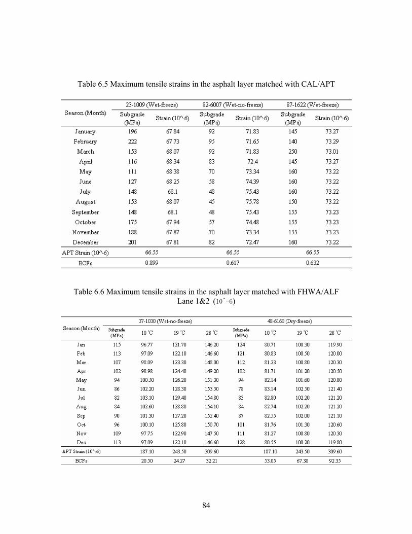
Table 6.5 Maximum tensile strains in the asphalt layer matched with CAL/APT
Table 6.6 Maximum tensile strains in the asphalt layer matched with FHWA/ALF
Lane 1&2 (10^-6)
84
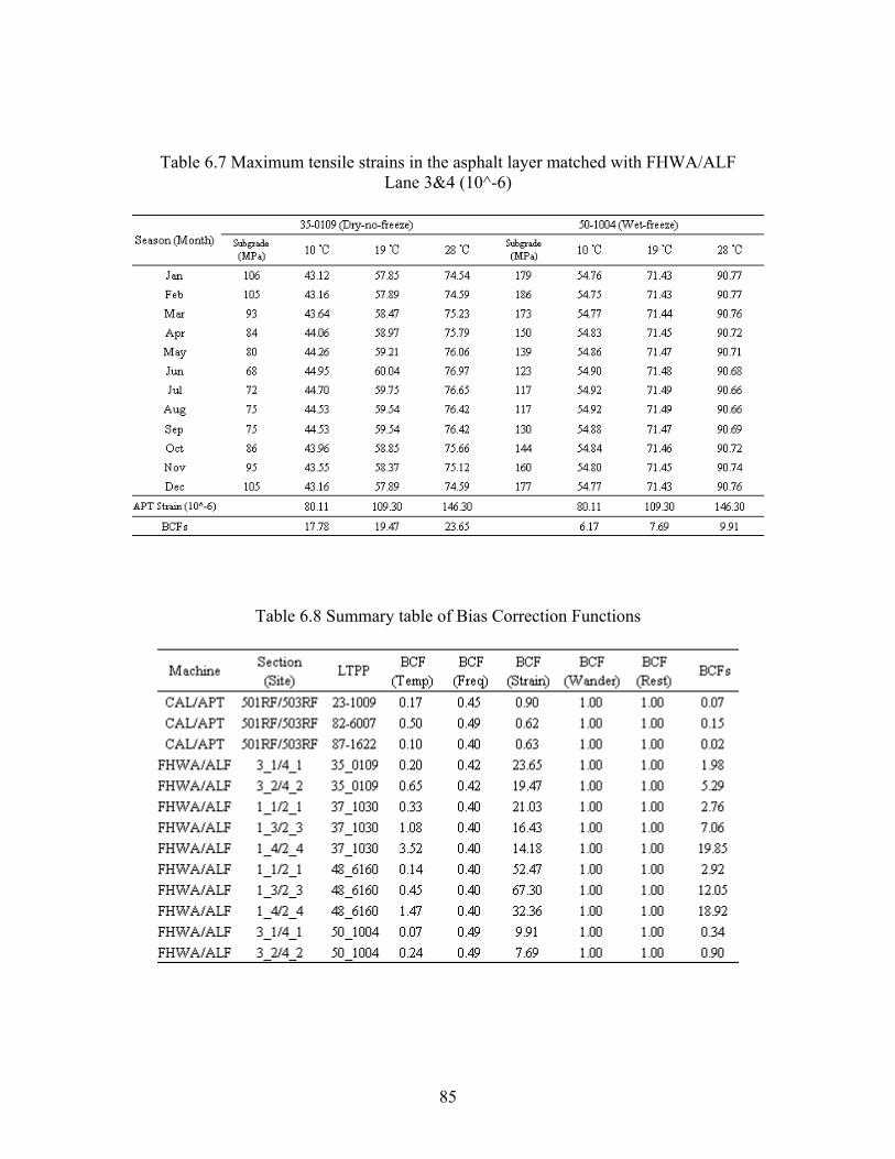
Table 6.7 Maximum tensile strains in the asphalt layer matched with FHWA/ALF
Lane 3&4 (10^-6)
Table 6.8 Summary table of Bias Correction Functions
85

Table 6.8 is a summary of all the Bias Correction Functions including the effects of
temperature, travel speed, traffic wandering, moisture condition and rest periods.
6.2 Marginal Shift Factor (M)
The marginal shift factor M to account for all other unquantifiable differences is
developed by combing APT and LTPP datasets. APT recorded the crack length under
different load repetitions while LTPP records the area. Since the fatigue distress
recording systems of APT and LTPP differ from each other, there is a need to standardize
the test results to make them compatible. The Damage Ratio (DR) concept is used in this
research, which is defined as the ratio of total crack length to the maximum crack length
when the whole area is cracked. According to LTPP distress identification manual, the
crack length of a fatigue area is usually less than 0.3 meters (FHWA, 2003). Accordingly,
the DR is defined as 100% when the cracked area is comprised of less than 0.3 meters
cracks (Figure 6.6).
Figure 6.6 Definition of a fully damaged fatigue cracking area (DR=1, crack density = 6.7m/m2 correspondingly)
86
In this research, the differences between APT and LTPP sites are captured by the
addressed variables. To account for all unquantifiable differences (such as aging)
between the performance of the pavement site under APT and in-service conditions, the
margin of shift factor M is calibrated by combining data sets as shown in Equation 3.2, M
will be calculated explicitly using the equation developed earlier:
( ) )log()log(log BAFM ×−= (6.6)
The APT performance data provide the distribution of log (A), while the data from
LTPP will provide the distribution of log (F). With the previously-mentioned log-normal
assumptions, the prediction error is a normal random variable with mean equal to zero,
together with the calculated B, margin of shift factor M is calibrated by means of
constrained regression analysis between log (F) and log (A×B). As shown in Figure 6.7,
when the coefficient before log (A×B) is constrained as 1, the intercept (constant part of
this regression) represents the expected value of log (M). If it is statistically significantly
different from zero, the marginal shift factor is necessary and can only be released when
all variables to account for the difference are included. In other words, M can be
calculated by minimizing the squared differences between Log (A×B) and Log (F).
87

Figure 6.7 Constrained regressions on marginal shift factor M
Table 6.9 presents the load repetitions (ESALs) of CAL/APT and FHWA/ALF to
different damage levels (damage ratio) of area cracked. Associated with that, load
repetitions of selected LTPP sites are collected at the same fatigue cracking level. It
should be noted that the accumulated load repetitions are not proportional to fatigue
cracking level, so the calibrated marginal shift M may be different according to different
failure criteria.
With the constrained regression analysis between log (F) and log (A×B), the
estimated intercept is 0.191. Then, the margin of shift, M, is estimated as 1.552 (i.e.
100.191) when 45% area cracked (3m/m2) is set as the failure criterion. This means that
despite the quantified differences, the APT program tends to predict shorter pavement
fatigue life. The fatigue performance of pavement is underestimated and this marginal
shift factor M should be included.
88
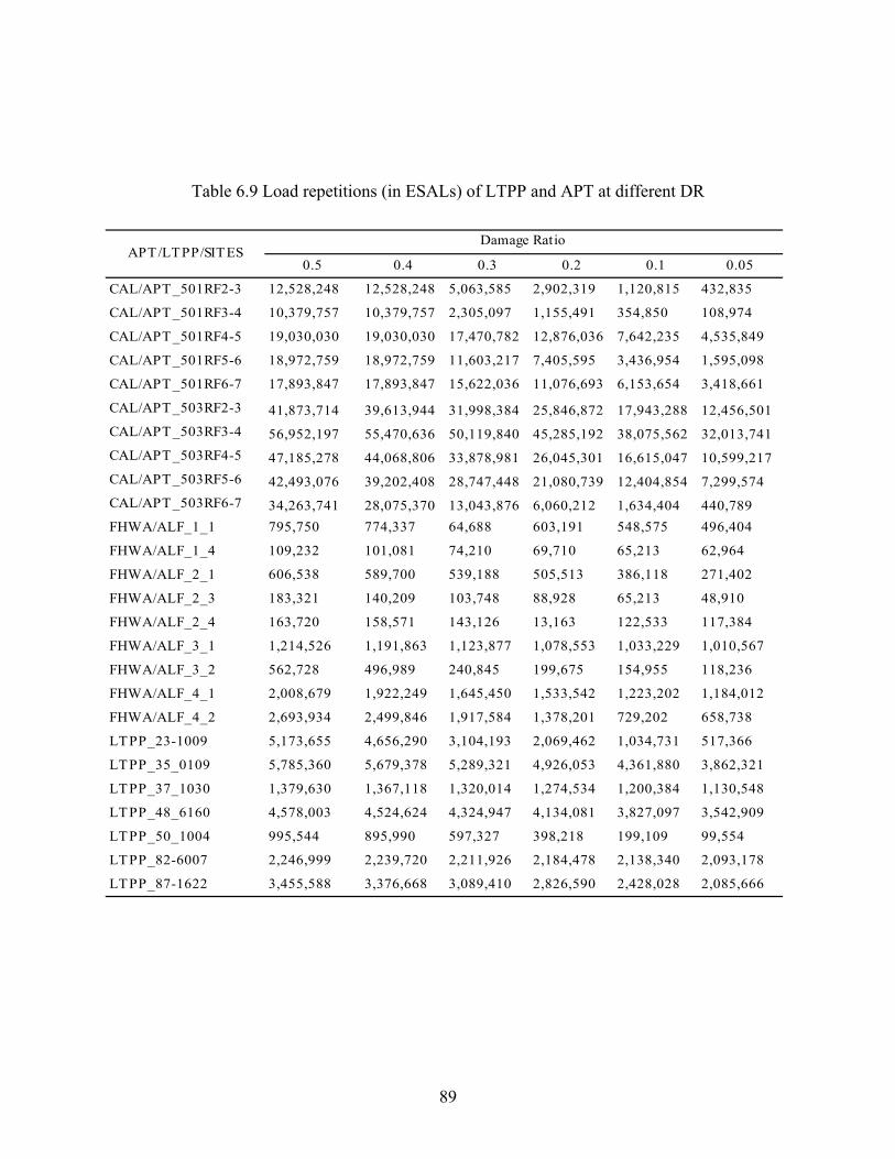
Table 6.9 Load repetitions (in ESALs) of LTPP and APT at different DR
0.5 0.4 0.3 0.2 0.1 0.05
CAL/APT_501RF2-3 12,528,248 12,528,248 5,063,585 2,902,319 1,120,815 432,835
CAL/APT_501RF3-4 10,379,757 10,379,757 2,305,097 1,155,491 354,850 108,974
CAL/APT_501RF4-5 19,030,030 19,030,030 17,470,782 12,876,036 7,642,235 4,535,849
CAL/APT_501RF5-6 18,972,759 18,972,759 11,603,217 7,405,595 3,436,954 1,595,098
CAL/APT_501RF6-7 17,893,847 17,893,847 15,622,036 11,076,693 6,153,654 3,418,661
CAL/APT_503RF2-3 41,873,714 39,613,944 31,998,384 25,846,872 17,943,288 12,456,501CAL/APT_503RF3-4 56,952,197 55,470,636 50,119,840 45,285,192 38,075,562 32,013,741CAL/APT_503RF4-5 47,185,278 44,068,806 33,878,981 26,045,301 16,615,047 10,599,217CAL/APT_503RF5-6 42,493,076 39,202,408 28,747,448 21,080,739 12,404,854 7,299,574CAL/APT_503RF6-7 34,263,741 28,075,370 13,043,876 6,060,212 1,634,404 440,789FHWA/ALF_1_1 795,750 774,337 64,688 603,191 548,575 496,404
FHWA/ALF_1_4 109,232 101,081 74,210 69,710 65,213 62,964
FHWA/ALF_2_1 606,538 589,700 539,188 505,513 386,118 271,402
FHWA/ALF_2_3 183,321 140,209 103,748 88,928 65,213 48,910
FHWA/ALF_2_4 163,720 158,571 143,126 13,163 122,533 117,384
FHWA/ALF_3_1 1,214,526 1,191,863 1,123,877 1,078,553 1,033,229 1,010,567
FHWA/ALF_3_2 562,728 496,989 240,845 199,675 154,955 118,236
FHWA/ALF_4_1 2,008,679 1,922,249 1,645,450 1,533,542 1,223,202 1,184,012
FHWA/ALF_4_2 2,693,934 2,499,846 1,917,584 1,378,201 729,202 658,738
LTPP_23-1009 5,173,655 4,656,290 3,104,193 2,069,462 1,034,731 517,366
LTPP_35_0109 5,785,360 5,679,378 5,289,321 4,926,053 4,361,880 3,862,321
LTPP_37_1030 1,379,630 1,367,118 1,320,014 1,274,534 1,200,384 1,130,548
LTPP_48_6160 4,578,003 4,524,624 4,324,947 4,134,081 3,827,097 3,542,909
LTPP_50_1004 995,544 895,990 597,327 398,218 199,109 99,554
LTPP_82-6007 2,246,999 2,239,720 2,211,926 2,184,478 2,138,340 2,093,178
LTPP_87-1622 3,455,588 3,376,668 3,089,410 2,826,590 2,428,028 2,085,666
Damage RatioAPT/LTPP/SITES
89

6.3 Reliability Based Fatigue Life Prediction
The prediction error is then given by:
)log()log()log()log( MBAF iiii −×−=ε (6.7)
Figure 6.8 is the histogram of log(εi). It is chosen to perform an Anderson-Darling
test for normality, which is a test based on the empirical cumulative distribution function
(Anderson and Darling, 1952). A P-value larger than 0.05 will fail to reject the null
hypothesis that the log(εi) follows normal distribution at a 95% confidence level (Figure
6.9). Thus the distribution of the error term can be evaluated with existing database,
which is as follows:
( )2265.0,0)log( N≈ε (6.8)
log (error)
Freq
uenc
y
0.60.40.20.0-0.2-0.4-0.6
9
8
7
6
5
4
3
2
1
0
M ean 0.00001576S tD ev 0.2654N 48
Figure 6.8 Histogram of log (εi)
The equation for fatigue life prediction is now updated as follows:
90

161.0)log(265.0)Wlog( T +×+×−= BAZ R (6.9)
log (error)
Perc
ent
0.750.500.250.00-0.25-0.50
99
95
90
80
70
60
50
40
30
20
10
5
1
Mean
0.827
0.00001576StDev 0.2654N 4A D 0.220P-Value
8
Figure 6.9 Probability plot of log (εi)
The reliability of the performance prediction is evaluated as the normal deviate ZR,
which is determined from standard normal probabilities table and, more conveniently,
from Table 6.10.
Table 6.10 Standard normal deviate for various levels of reliability
Reliability (%)Standard normal
deviate (ZR) Reliability (%)Standard normal
deviate (ZR)
50 0 92 1.40555 0.126 93 1.47660 0.253 94 1.55565 0.385 95 1.64570 0.524 96 1.75175 0.674 97 1.88180 0.842 98 2.05485 1.036 99 2.32690 1.282 99.5 2.57691 1.341 99.9 3.09
91
Chapter 7: Validation of the Fatigue Life Prediction
7.1 Principles of Validation
The proposed approach should be validated using different dataset to examine the
predictive capacity and accuracy. Comparison of the model distress predictions to
observed distress were made by applying the following steps: (1) assemble a database of
in-service pavements and test sites, containing information regarding design, material,
construction, climate, traffic, and measure pavement distress in the form of fatigue
cracking; (2) for each test pavement, run the distress model using the data assembled in
step 1; and (3) compare the predicted distress to measured distress from the in-service test
sections and evaluate the predictive capacity and accuracy of the model.
The predictive capacity and accuracy of the distress model was evaluated using
statistical analysis as follows: (1) determine the correlation between predicted and
measured distress (R2); (2) determine the residual error between predicted and measured
distress (mean square error, MSE); and (3) use paired t-test to determine whether there is
a significant difference on average between measured and predicted distress for the
in-service pavements analyzed.
92
7.2 Data Gathering and Processing
A dataset different from that used for methodology development was prepared for
the validation of fatigue life prediction. A comprehensive search and review of
publications documenting the performance of in-field and in-service pavements was the
first task undertaken to conduct this study. Several studies, implementation projects and
investigation programs were identified as potential sources of data. Based on the type,
quality and potential usage of the data available, two programs were considered for
inclusion in this study. Details of each of these programs are presented in the following
sections.
7.2.1 APT Performance Data (FHWA/ALF)
In 2002, twelve lanes of full scale pavement were constructed at the FHWA’s
pavement testing facility to study the performance of Superpave mixtures containing
modified asphalt binders. Lane 2 used unmodified asphalt binder, and this lane served as
the control reference section. For this research, test results pertaining to FHWA/ALF lane
2 site 3 were utilized. Details of the structural and material properties of these test
sections can be found in Figure 7.1. Additional information can be found in Qi et al.
(2004).
The progressive cracking patterns in terms of the cracked area are shown in Figure
7.2.
93

Figure 7.1 Layout of part of the 12 pavement test lanes
Figure 7.2 Performance fatigue data corresponding to Lane 2 site 3
94

7.2.2 In-service pavement performance data
The main source for in-service pavement data selected to conduct the validation was
the Long Term Pavement Performance database (LTPP). The LTPP database is part of a
comprehensive program established by the Strategic Highway Research Program
designed specifically to investigate the long-term performance of various pavement
structures, both new and rehabilitated, subject to different loads, environments, subgrade
soils, and maintenance practices. This thorough program consists of over 2,400 pavement
test sections of in-service, new and rehabilitated pavements located across the United
States, Canada and Puerto Rico. These pavement sections are classified in the LTPP
program as General Pavement Studies (GPS) or Specific Pavement Studies (SPS).
Essentially, the main difference between them is that the GPS test sections are existing
pavements at the start of the program and the SPS test sections are newly constructed
sections or existing pavement sections subject to maintenance or rehabilitation
treatments. Regardless of what experiment classification a test section pertains to, similar
data is housed within the database. This data includes original construction data,
inventory data, material data, performance data and climatic information.
As one of the main LTPP products, the LTPP DataPave Online web-page provides
fast and easy means for navigating the complex structure of the LTPP relational database.
One of the principal advantages of this database management system is that it allowed the
generation of summary reports of the pavement information. In addition, in order to
obtain the latest updates of the data, performance data was retrieved from the LTPP
95
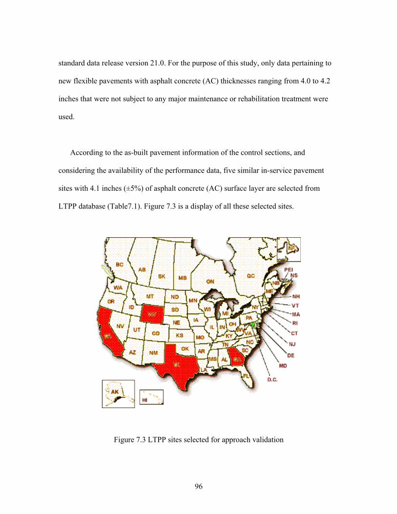
standard data release version 21.0. For the purpose of this study, only data pertaining to
new flexible pavements with asphalt concrete (AC) thicknesses ranging from 4.0 to 4.2
inches that were not subject to any major maintenance or rehabilitation treatment were
used.
According to the as-built pavement information of the control sections, and
considering the availability of the performance data, five similar in-service pavement
sites with 4.1 inches (±5%) of asphalt concrete (AC) surface layer are selected from
LTPP database (Table7.1). Figure 7.3 is a display of all these selected sites.
Figure 7.3 LTPP sites selected for approach validation
96

Table 7.1 Selected LTPP sites match FHWALF program
7.3 Verification and Validation Analysis of the Proposed Fatigue Life Prediction
In order to check the prediction accuracy of the aforementioned model, a verification
and validation study was conducted. For this study, verification and validation were
defined as follows:
97
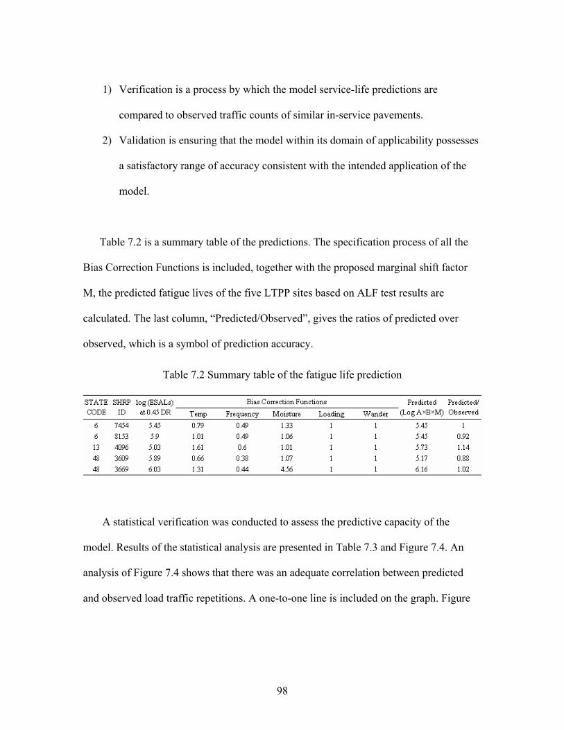
1) Verification is a process by which the model service-life predictions are
compared to observed traffic counts of similar in-service pavements.
2) Validation is ensuring that the model within its domain of applicability possesses
a satisfactory range of accuracy consistent with the intended application of the
model.
Table 7.2 is a summary table of the predictions. The specification process of all the
Bias Correction Functions is included, together with the proposed marginal shift factor
M, the predicted fatigue lives of the five LTPP sites based on ALF test results are
calculated. The last column, “Predicted/Observed”, gives the ratios of predicted over
observed, which is a symbol of prediction accuracy.
Table 7.2 Summary table of the fatigue life prediction
A statistical verification was conducted to assess the predictive capacity of the
model. Results of the statistical analysis are presented in Table 7.3 and Figure 7.4. An
analysis of Figure 7.4 shows that there was an adequate correlation between predicted
and observed load traffic repetitions. A one-to-one line is included on the graph. Figure
98
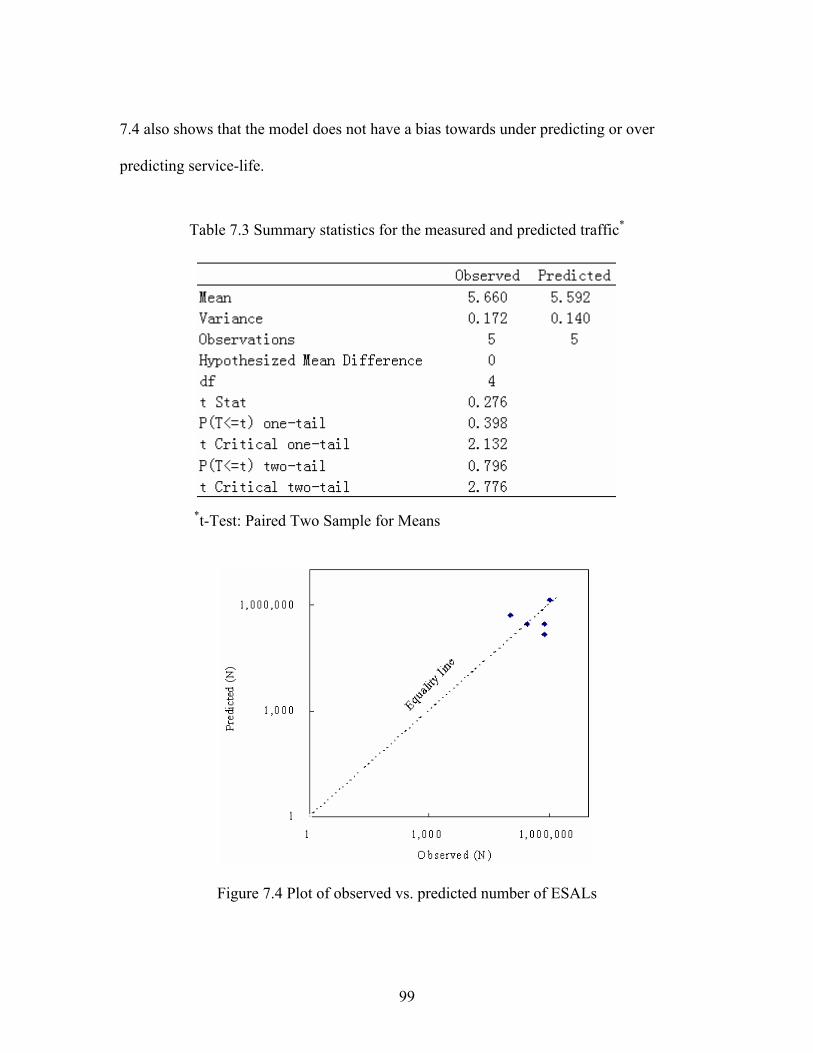
7.4 also shows that the model does not have a bias towards under predicting or over
predicting service-life.
Table 7.3 Summary statistics for the measured and predicted traffic*
*t-Test: Paired Two Sample for Means
Figure 7.4 Plot of observed vs. predicted number of ESALs
99

Furthermore, an analysis of the summary statistics proves that the null hypothesis that
the average of the differences between the paired observations is zero could not be
rejected.
The proposed approach for fatigue life prediction is valid.
100
Chapter 8: Summary, Conclusions and Future Work
8.1 Summary
The main objective of this research is to analyze and quantify the difference between
APT and in-service pavements and their impacts on the overall pavement fatigue life. To
achieve this objective, a methodology framework for using results for APT to predict the
life of in-service pavements has been presented. The methodology proposed in this
research is generic, independent of facility, conditions or environment. However, it has
been initially calibrated for the specific set of data available at this time, (Caltrans APT
programs, FHWA’s ALF program and LTPP Studies). By applying this methodology,
APT performance results from a structure similar to an in-service structure can be used to
run limited third-point bending tests and computer simulations in order to obtain an
accurate estimate of the necessary Bias Correction Factors to estimate in-service
performance. This methodology represents a significant improvement on the current
state-of-practice and enables more accurate pavement performance predictions. The
methodology enables not only the estimation of mean expected performance but also its
expected variability (standard deviation), thus facilitating the implementation of
reliability-based predictions and the incorporation of risk.
101
8.2 Conclusions
From the results of tests and associated analyses, the following preliminary
conclusions have been established. It is expected that these conclusions may change as
further data are incorporated into the analysis. The LTPP program will end in 2009 and as
the final database is compiled, there will be an invaluable opportunity to enhance and
validate the models developed in this dissertation. The work on this regard is not
complete but this methodology represents an important step in the right direction. To
date, the most significant findings can be summarized as follows:
1) Some of the important factors that help to explain the differences between the
performance of APT sites and LTPP sites have been recognized and evaluated.
These factors include: loading frequency (loading speed), loading ratio (rest
period), traffic wandering, seasonal moisture change, and pavement temperature.
The factors are individually assessed instead of being aggregated into one “shift
factor” as is generally done.
2) Based on laboratory third-point beam fatigue test results, a general model relating
pavement temperature and loading frequency to the difference of fatigue life
between APT and in-service pavement was developed. The model shows that
pavement temperature contributes the most to the difference. The most significant
advantage of this model is that it is based on the observed fatigue life in the
102
laboratory as opposed to current models that estimate life based on the dynamic
modulus. In addition, dynamic stiffness is preferred because it correlates closely
to fatigue performance.
3) Heavier and faster traffic has been proven to have a negative impact on pavement
performance, reducing the fatigue life. A heavier truck generates larger strains at
the bottom of the asphalt layer, thus resulting in shorter fatigue life. According to
these preliminary results, higher loading frequency (all else being equal) results in
higher material stiffness and, therefore, in higher stress levels and shorter fatigue
lives under the strain-controlled test. It should be noted that these results apply to
thin asphalt structures (asphalt surface on granular base); however, the results
may be opposite for full-depth asphalts (asphalt surface and asphalt base). The
evaluation of thick asphalt layers was out of the scope of the current dissertation
because of the lack of APT and field data. These findings are practical for
pavements in use in Texas; the pavement life would be greatly shortened due to
heavy and high speed traffic.
4) Traffic-induced pavement strains vary with the modulus of various pavement
layers. The effect of differential moisture conditions between APT and in-service
pavements relates primarily to the loss of support of the asphalt concrete base or
surface and the consequential increase in tensile strains for the same applied
wheel loads. For the same applied wheel loads, the tensile strains at the bottom of
103
asphalt concrete layer may increase significantly due to the loss of support from
subgrade. The results show that the seasonal water content variations of subgrade
affect the estimation of pavement fatigue life conditionally: the poorer the
pavement structure, the greater the effect will be.
5) Rest periods have been proven to have a beneficial effect on pavement fatigue
life. Rest periods in an APT experiment are shorter than those occurring on
actual highways, resulting in a longer fatigue life of in-service pavement for the
same traffic volume. The benefits seem to reach a maximum when the rest period
equals to 25 times the load cycle. Unfortunately, for the cases studied, the loading
ratios were larger than 25, and therefore the corresponding BCF were similar. The
methodology, however, allows the determination when the loading ratios in the
field are variable. This can be assessed by including urban highways where traffic
congestion will cause differential loading ratio during the day.
6) Because of the inability to quantify all variables that affect the differences of
overall pavement fatigue life between APT and in-service pavement, a marginal
shift factor, M, should be introduced at this time. For the cases studied, this factor
was estimated as 1.552. This research represents a significant improvement on
pavement performance prediction. This marginal shift cannot be ignored and will
only be released in the future when all the differences are taken into account. The
104

APT sections tend to present shorter pavement fatigue life and the fatigue
performance of pavement is underestimated.
7) Sensitivity analyses were performed to numerically determine the effects of
temperature, loading speed, lateral wander, rest period and subgrade moisture
content. The fatigue life of flexible pavement is very sensitive to temperature
change. On average, and for the cases studied in this dissertation, the following
conclusions are valid:
a) Increasing the temperature from -10 ℃ to 10℃ will result in fatigue life
extension by as much as 14 times, indicating that the fatigue life of flexible
pavement is very sensitive to temperature change.
b) One km/hour increase of driving speed will result in about 1% decrease of
pavement fatigue life based on this research.
c) A unity increase of the loading ratio results in an increase of 2.6% of
pavement fatigue life on average but this beneficial effect reaches a maximum
when the loading ratio reaches 25.
d) Increasing the standard deviation of lateral wandering from 0.05 m to1.5 m
may increase the fatigue life by as much as 12 times, indicating that the
fatigue life of flexible pavement is very sensitive to standard deviation of
lateral position.
e) Validation process proved that the proposed approach for fatigue life
prediction is valid.
105

8.3 Methodology Limitations and Further Research
Due to the lack of data, there is a main difference between APT and in service
pavements not addressed in this research, which contributes the most to the marginal shift
factor M. The difference not addressed is material aging properties of in service
pavement. This aspect has effect on pavement fatigue performance and should be
calibrated into future work.
106

Appendix A: Specification of the Bias Correction Functions
A.1 Specification of General Bias Correction Function
All these correction functions are aimed at capturing the overall differential effect of
the specified variable between in-service pavements and similar pavements subjected to
APT, which is represented by the ratio of the expected performance of the mixes under
the conditions in the field over the expected performance of the mixes under APT
conditions, as in Equation A.1.
inf
APTf
APTf
inf
DD
NN
BCFgeneric == (A.1)
Since the variable of interest may be in different levels (under different conditions),
and under different loading and environmental conditions pavement structure performs
differently, there is a need to account for the overall damage under all the levels. Miner’s
law was used in the development of the Bias Correction Functions. To account for the
difference and the overall damage ascended, a particularly convenient form known as
Linear Cumulative Damage (Miner’s law) was proposed. The life of a pavement
experiencing fatigue at various situations can be assessed through the cumulative damage
(D) as follows:
∫∫=
inin
APTAPTgeneric dxxfinD
dxxfAPTDBCF)()(
)()(
(A.2)
107

Given that the fatigue life of a pavement structure under condition xin.i is , the
damage of one pass of traffic loading to pavement structure from condition x
)( .a
iinxg
i can be
expressed as:
Damage of one pass from condition xin.i )(
1
.. a
iiniin xg
D == (A.3)
Where,
xin: variable of interest under in-service conditions,
α: parameter that reflects the sensitivity of a particular process to a change in the
level of variable x. This parameter represents the order of the moment,
g(x): fatigue life as a function of variable x, and
Provided the portion in condition xin.i is , the overall damage of one pass of
traffic loading to pavement structure from all conditions can be expressed as the
summary of all the damages:
)( .iinxf
Damage of one pass = iinaiin
iin dxxg
xf.
.
.
)()(1
∫×
iiniina
iin dxxfxg ..1
. )()]([∫= − (A.4)
So the fatigue life of a pavement structure under all conditions is the reciprocal of the
overall damage of one pass of traffic loading:
iiniin
aiin
in dxxfxgN
..1
. )()]([1
∫=
− (A.5)
108

In principle, this Bias Correction Function is the ratio of the expected performance of
the pavement structure under the conditions in the field over the expected performance of
the pavement structure under APT conditions, therefore,
∫
∫=
−
−
APTAPTAPT
iiniina
iingeneric
dxxfxg
dxxfxgBCF
)()]([1
)()]([1
1
..1
.
α
∫
∫=
−
−
iiniina
iin
APTAPTAPT
dxxfxgdxxfxg
..1
.
1
)()]([)()]([ α
(A.6)
If the portion in condition xi is given as probability mass function and the
condition of a controlled APT is uniform, the Bias Correction Function can then be
simplified as:
)( .iinxp
∑
∑=
=
−
=
−
n
Iiiniin
m
JJAPT
aAPT
generic
xpxg
xpxgBCF
1.
1
.
1,
1
)()]([
)()]([
α (A.7)
A.2 Specification of Bias Correction Function for Moisture
The change of subgrade moisture content relates primarily to the variation of the
strength of the subgrade and, therefore, to the bottom tensile strains of asphalt concrete
layer. The fatigue life as a function of the bottom tensile strains can be expressed as:
8.41
−= εkN f (A.8)
And based on the general form the Bias Correction Function for Moisture is:
109
∑=
=
−
−
n
Iiiniin
APTmoisture
xpxg
xgBCF
1.
1
.
1
)()]([
)]([α
α
=∑=
−−
−−
n
Iiiniin
APT
xpk
k
1.
18.4,1
18.41
)(][
][
ε
ε
=∑=
n
Iiiniin
APT
xp1
.8.4,
8.4
)(ε
ε (A.9)
If a whole year is divided into 12 seasons to represent different subgrade moisture
conditions, the Bias Correction Function for Moisture should be:
∑=
=
12
1
8.4,
8.412
Iiin
APTmoistureBCF
ε
ε (A.10)
A.3 Specification of Bias Correction Function for Temperature
A regression equation based on laboratory four-point bending fatigue test results
shows fatigue life as a function of temperature was developed as follows:
Tf kN 057.0
210= (A.11)
Since pavement temperature varies hourly and daily, and the traffic volume changes
hourly ( ), the Bias Correction Function for Temperature should account for all three
variables. Still based on the general form the function is developed as follows:
ia
∑=
=
−
−
n
Iiiniin
APTeTemperatur
xpxg
xgBCF
1.
1
.
1
)()]([
)]([α
α
110

111
=∑ ×∑=
−
=
−
24
1
1.057.02
1
1057.02
3651]10[
]10[
ii
ijinT
j
APTT
ak
k365
=∑ ×∑=
−−
=
24
1
).(0570.0
110
365
ii
APTTijinT
ja
LRf kN 011.0
310
A regression equation based on the research of the effect of rest period on fatigue
performance shows fatigue life as a function of loading ratio as follows:
A.4 Specification of Bias Correction Function for Loading Ratio
Since traffic loading ratio varies hourly and yearly, the Bias Correction Function for
loading ratio should account for these. The function is developed as follows:
=
∑=
=
−
n
Iiiniin
APToLadingRati
xg
xgBCF
1..
1
))]([
)]([α
α
=
=
∑∑=
−−
=
24
1
).(011.0
110
24
i
PTLRAijinLRn
j
n
∑ ××∑=
−
=
−
24
1
1.011.03
1
1011.03
241]10[
]10[
i
ijinLRn
j
APTLR
k
k1n
365 (A.12)
(A.13)
− xp1 (
(A.14)
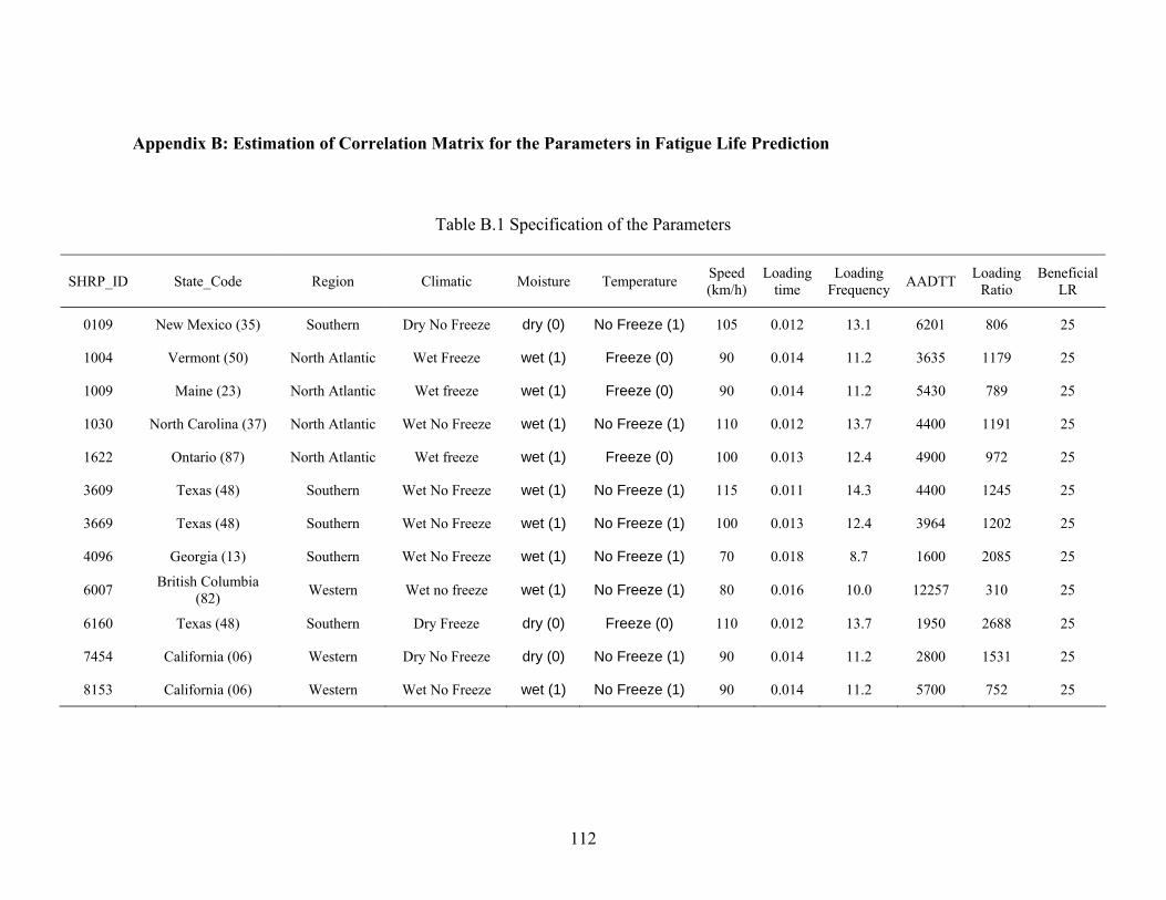
Appendix B: Estimation of Correlation Matrix for the Parameters in Fatigue Life Prediction
Table B.1 Specification of the Parameters
SHRP_ID State_Code Region Climatic Moisture Temperature Speed (km/h)
Loading time
Loading Frequency AADTT Loading
Ratio Beneficial
LR
0109 New Mexico (35) Southern Dry No Freeze dry (0) No Freeze (1) 105 0.012 13.1 6201 806 25
1004 Vermont (50) North Atlantic Wet Freeze wet (1) Freeze (0) 90
0.014 11.2 3635 1179 25
1009 Maine (23) North Atlantic Wet freeze wet (1) Freeze (0) 90 0.014 11.2 5430 789 25
1030 North Carolina (37) North Atlantic Wet No Freeze wet (1) No Freeze (1) 110 0.012 13.7 4400 1191 25
1622 Ontario (87) North Atlantic Wet freeze wet (1) Freeze (0) 100 0.013 12.4 4900 972 25
3609 Texas (48) Southern Wet No Freeze wet (1) No Freeze (1) 115 0.011 14.3 4400 1245 25
3669 Texas (48) Southern Wet No Freeze wet (1) No Freeze (1) 100 0.013 12.4 3964 1202 25
4096 Georgia (13) Southern Wet No Freeze wet (1) No Freeze (1) 70 0.018 8.7 1600 2085 25
6007 British Columbia (82) Western Wet no freeze wet (1) No Freeze (1) 80 0.016 10.0 12257 310 25
6160 Texas (48) Southern Dry Freeze dry (0) Freeze (0) 110 0.012 13.7 1950 2688 25
7454 California (06) Western Dry No Freeze dry (0) No Freeze (1) 90 0.014 11.2 2800 1531 25
8153 California (06) Western Wet No Freeze wet (1) No Freeze (1) 90 0.014 11.2 5700 752 25
112
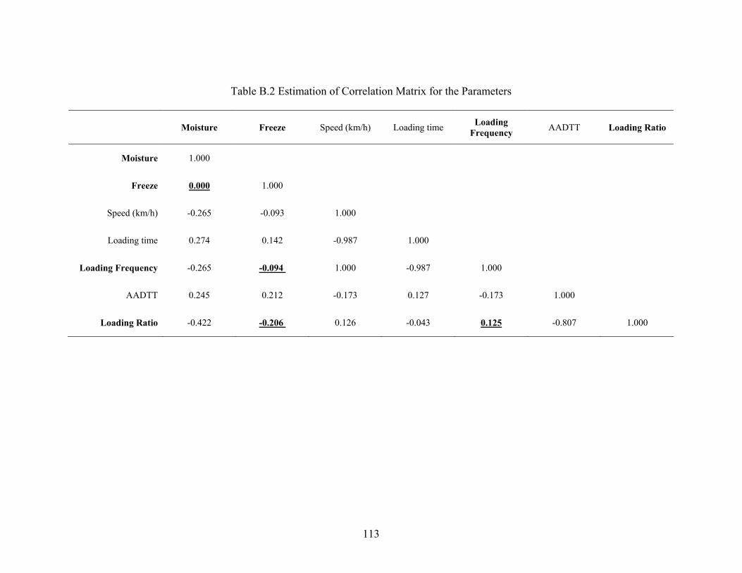
Table B.2 Estimation of Correlation Matrix for the Parameters
Moisture Freeze Speed (km/h) Loading time Loading Frequency AADTT Loading Ratio
Moisture 1.000
Freeze 0.000 1.000
Speed (km/h) -0.265 -0.093 1.000
Loading time 0.274 0.142 -0.987 1.000
Loading Frequency -0.265 -0.094 1.000 -0.987 1.000
AADTT 0.245 0.212 -0.173 0.127 -0.173 1.000
Loading Ratio -0.422 -0.206 0.126 -0.043 0.125 -0.807 1.000
113
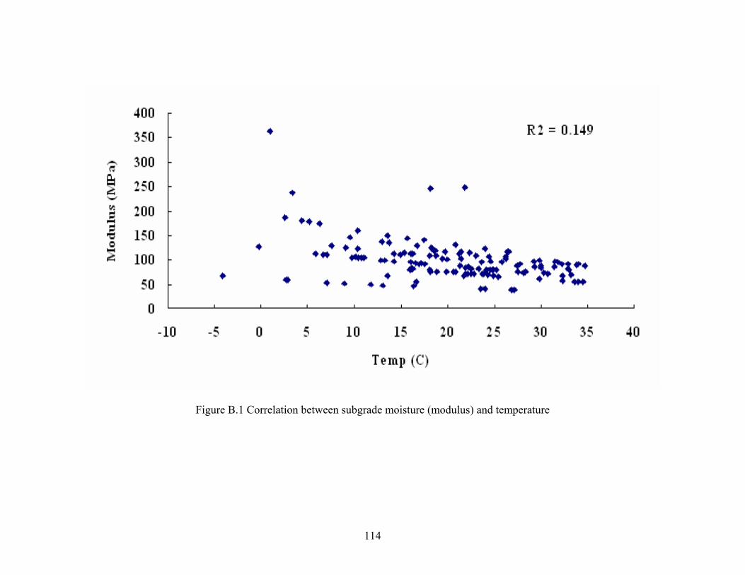
114
Figure B.1 Correlation between subgrade moisture (modulus) and temperature
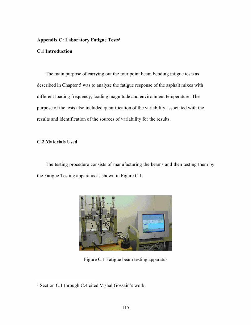
Appendix C: Laboratory Fatigue Tests1
C.1 Introduction
The main purpose of carrying out the four point beam bending fatigue tests as
described in Chapter 5 was to analyze the fatigue response of the asphalt mixes with
different loading frequency, loading magnitude and environment temperature. The
purpose of the tests also included quantification of the variability associated with the
results and identification of the sources of variability for the results.
C.2 Materials Used
The testing procedure consists of manufacturing the beams and then testing them by
the Fatigue Testing apparatus as shown in Figure C.1.
Figure C.1 Fatigue beam testing apparatus
1 Section C.1 through C.4 cited Vishal Gossain’s work.
115
The 36 tests consisted of premanufactured mixes designated as Accelerated
Pavement Testing (APT) mixes obtained from the pavement constructed at the J.J. Pickle
Research Campus (PRC) for Accelerated Pavement Testing with the Texas Mobile Load
Simulator (TxMLS).
C.3 AASHTO TP – 8
The AASHTO TP-8 (AASHTO TP8, 1996) standard provides procedures for
determining the fatigue life and fatigue energy of 380 mm long by 50 mm thick by 63
mm wide hot mix asphalt (HMA) beam specimens sawed from laboratory or field
compacted HMA and subjected to repeated flexural bending until failure. The fatigue life
and failure energy determined by this standard can be used to estimate the fatigue life of
HMA pavement layers under repeated traffic loading.
The four point beam bending test procedure (constant strain) involves applying
repeated loading and unloading on a beam specimen till the flexural stiffness of the
specimen reduces to a calculated value. One such application of loading and unloading is
termed as a load cycle.
The load is so applied that the specimen experiences a constant level of strain during
each loading cycle. Repeated sinusoidal loading at a frequency range of 2.5 to 20 Hz is
usually applied subjecting specimens to four points bending with free rotation and
116
horizontal translation at all load and reaction points with the flexural stiffness estimated
after every 10 cycles. The constant strain level can be fixed from 250-750 micro strains
as specified by AASHTO TP – 8. The flexural stiffness measured after the first 50
conditioning cycles is termed as initial stiffness and 50% of the initial stiffness is termed
as termination stiffness or point of failure. The test is stopped after the termination
stiffness has been achieved.
C.4 Manufacture of Beams
The asphalt mixes used for the construction of the section for Accelerated Pavement
Testing at PRC were transported to the laboratories for testing.
AASHTO TP – 8 specifies the desired void content of 7 ± 0.5 % in the beam, which
is representative of the void content of a new pavement. Based on the void content, the
amount of mix to be compacted to a specified volume can be computed by volumetric
calculations. The volume is determined based on the volume of the mold used for
compaction. The mold is made out of steel with a width of 152.4 mm and length of 393.7
mm, and is supplied with the Asphalt Vibratory Compactor (AVC). The amount of
aggregate blend can then be calculated from the amount of mix as the percentage of
binder by mass of mix is known. The amounts of individual aggregates required to
prepare the blend are then calculated from the amount of blend. The various volumetric
117

equations involved are listed as Equations (C.1) – (C.5). A conservative value of Gmm is
used in the calculations.
b
sbb P
MPM
−=
1*
(C.1)
bst MMM += (C.2)
V = l * b * h (C.3)
VM
G tmb =
(C.4)
mm
mb
GG
VIM −=1 (C.5)
Where,
Mb: Mass of binder
Mt: Total mass of mix
Pb: Percentage of binder by weight of the mix
Ms: Mass of aggregate
l ,b,h: Dimensions of the mold
V: Volume of the mold
Gmb: Bulk density
Gmm: Maximum theoretical specific gravity
VIM: Voids in mix
Thus, it is essentially a backcalculation procedure to estimate Ms based on a known
VIM. After determining the Ms, the desired proportions of the aggregates are mixed and
then heated to the mixing temperatures.
118

The mix is then aged in the oven for 4 hours at 135 ℃ to simulate the aging in the
field in the time taken to transport the mix from the plant to the pavement. Two thousand
grams of the mix is taken out (in total) from the pans after 4 hours for tests to determine
theoretical maximum density in accordance with AASHTO T 209 (AASHTO T 209, 99).
Figure C.2 Rotatory mixer for mixing binder with aggregates
AASHTO T 209 test method covers the determination of the theoretical maximum
specific gravity and density of uncompacted bituminous paving mixtures at 25°C. The
obtained rice value (Gmm, maximum theoretical specific gravity) is then used to estimate
the mass of the mix required to achieve the desired void content based on volumetric
calculations. The mix is then heated to the compaction temperature.
119
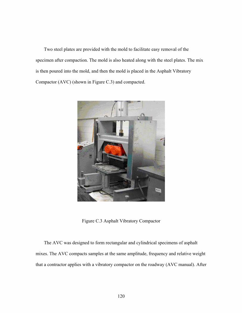
Two steel plates are provided with the mold to facilitate easy removal of the
specimen after compaction. The mold is also heated along with the steel plates. The mix
is then poured into the mold, and then the mold is placed in the Asphalt Vibratory
Compactor (AVC) (shown in Figure C.3) and compacted.
Figure C.3 Asphalt Vibratory Compactor
The AVC was designed to form rectangular and cylindrical specimens of asphalt
mixes. The AVC compacts samples at the same amplitude, frequency and relative weight
that a contractor applies with a vibratory compactor on the roadway (AVC manual). After
120

the samples are compacted, they are extracted with the help of an air cylinder. After
extraction, the top plate is immediately removed. The slab is kept on a flat surface for
10-12 minutes to cool down, and then the bottom plate is also removed. After
compaction, the slabs are left overnight and then tested for their bulk density.
The slabs are then sawed to derive two beams 380 mm long (L) by 50 mm high (h)
by 63 mm wide (b) out of each slab, which serve as replicates. The slabs are cut such that
each side is sawed. The beams are then aged for 7 days in a temperature control chamber
at 20 ℃. They are then tested in accordance with AASHTO TP – 8. The strain levels and
the loading frequency were selected based on experimentation discussed in Chapter 5.
The test was terminated at a stiffness level of 20% instead of the traditional 50%.
The beam is subjected to both tension and compression in a constant strain test. It
can be observed in Figure C.4 that the strain is not in phase with the load indicating the
viscoelastic nature of asphalt, and the difference represents the phase angle of asphalt
binder. The phase angle provides a relative indication of the viscous and elastic behavior
of the asphalt binder. Materials with a phase angle of 90 degrees are completely viscous;
while materials with a phase angle of 0 degrees are completely elastic. At intermediate
temperatures, such as 20ºC, asphalt binders are said to be viscoelastic (phase angle near
45 degrees).
121
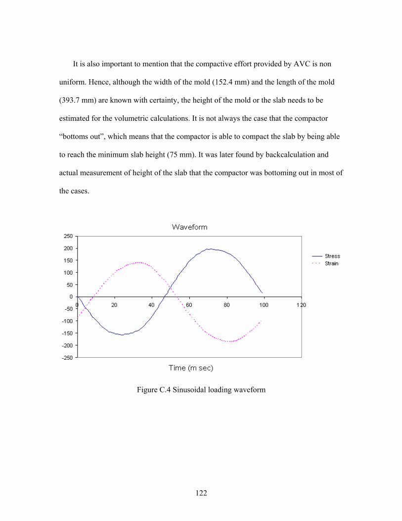
It is also important to mention that the compactive effort provided by AVC is non
uniform. Hence, although the width of the mold (152.4 mm) and the length of the mold
(393.7 mm) are known with certainty, the height of the mold or the slab needs to be
estimated for the volumetric calculations. It is not always the case that the compactor
“bottoms out”, which means that the compactor is able to compact the slab by being able
to reach the minimum slab height (75 mm). It was later found by backcalculation and
actual measurement of height of the slab that the compactor was bottoming out in most of
the cases.
Figure C.4 Sinusoidal loading waveform
122

Figure C.5 is a sample fatigue test record (Beam APT 5-2-1 10Hz@30C 600ue). Tables C.1 through C.9 are summary
tables of all the laboratory fatigue test results at different remaining material stiffness.
Figure C.5 Sample fatigue test record (Beam APT 5-2-1 10Hz at 30C 600ue)
123
C.5 Laboratory fatigue test results
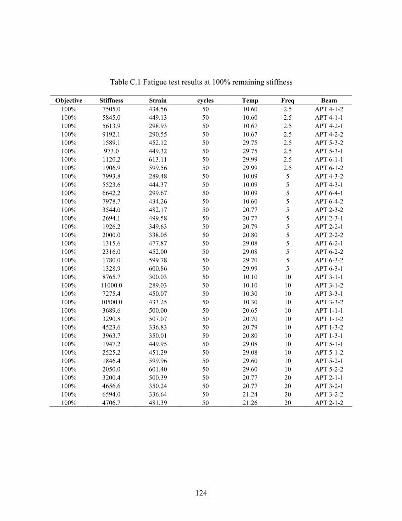
Table C.1 Fatigue test results at 100% remaining stiffness
Objective Stiffness Strain cycles Temp Freq Beam 100% 7505.0 434.56 50 10.60 2.5 APT 4-1-2 100% 5845.0 449.13 50 10.60 2.5 APT 4-1-1 100% 5613.9 298.93 50 10.67 2.5 APT 4-2-1 100% 9192.1 290.55 50 10.67 2.5 APT 4-2-2 100% 1589.1 452.12 50 29.75 2.5 APT 5-3-2 100% 973.0 449.32 50 29.75 2.5 APT 5-3-1 100% 1120.2 613.11 50 29.99 2.5 APT 6-1-1 100% 1906.9 599.56 50 29.99 2.5 APT 6-1-2 100% 7993.8 289.48 50 10.09 5 APT 4-3-2 100% 5523.6 444.37 50 10.09 5 APT 4-3-1 100% 6642.2 299.67 50 10.09 5 APT 6-4-1 100% 7978.7 434.26 50 10.60 5 APT 6-4-2 100% 3544.0 482.17 50 20.77 5 APT 2-3-2 100% 2694.1 499.58 50 20.77 5 APT 2-3-1 100% 1926.2 349.63 50 20.79 5 APT 2-2-1 100% 2000.0 338.05 50 20.80 5 APT 2-2-2 100% 1315.6 477.87 50 29.08 5 APT 6-2-1 100% 2316.0 452.00 50 29.08 5 APT 6-2-2 100% 1780.0 599.78 50 29.70 5 APT 6-3-2 100% 1328.9 600.86 50 29.99 5 APT 6-3-1 100% 8765.7 300.03 50 10.10 10 APT 3-1-1 100% 11000.0 289.03 50 10.10 10 APT 3-1-2 100% 7275.4 450.07 50 10.30 10 APT 3-3-1 100% 10500.0 433.25 50 10.30 10 APT 3-3-2 100% 3689.6 500.00 50 20.65 10 APT 1-1-1 100% 3290.8 507.07 50 20.70 10 APT 1-1-2 100% 4523.6 336.83 50 20.79 10 APT 1-3-2 100% 3963.7 350.01 50 20.80 10 APT 1-3-1 100% 1947.2 449.95 50 29.08 10 APT 5-1-1 100% 2525.2 451.29 50 29.08 10 APT 5-1-2 100% 1846.4 599.96 50 29.60 10 APT 5-2-1 100% 2050.0 601.40 50 29.60 10 APT 5-2-2 100% 3200.4 500.39 50 20.77 20 APT 2-1-1 100% 4656.6 350.24 50 20.77 20 APT 3-2-1 100% 6594.0 336.64 50 21.24 20 APT 3-2-2 100% 4706.7 481.39 50 21.26 20 APT 2-1-2
124
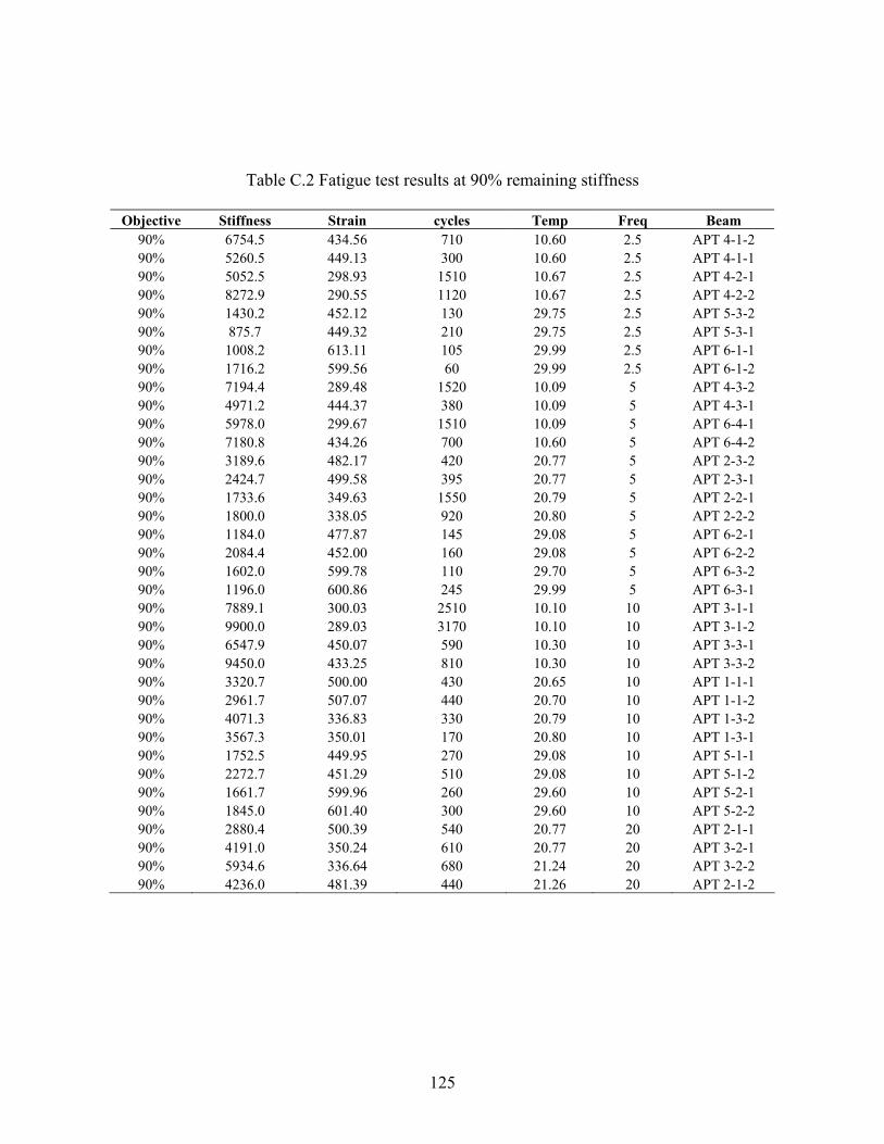
Table C.2 Fatigue test results at 90% remaining stiffness
Objective Stiffness Strain cycles Temp Freq Beam 90% 6754.5 434.56 710 10.60 2.5 APT 4-1-2 90% 5260.5 449.13 300 10.60 2.5 APT 4-1-1 90% 5052.5 298.93 1510 10.67 2.5 APT 4-2-1 90% 8272.9 290.55 1120 10.67 2.5 APT 4-2-2 90% 1430.2 452.12 130 29.75 2.5 APT 5-3-2 90% 875.7 449.32 210 29.75 2.5 APT 5-3-1 90% 1008.2 613.11 105 29.99 2.5 APT 6-1-1 90% 1716.2 599.56 60 29.99 2.5 APT 6-1-2 90% 7194.4 289.48 1520 10.09 5 APT 4-3-2 90% 4971.2 444.37 380 10.09 5 APT 4-3-1 90% 5978.0 299.67 1510 10.09 5 APT 6-4-1 90% 7180.8 434.26 700 10.60 5 APT 6-4-2 90% 3189.6 482.17 420 20.77 5 APT 2-3-2 90% 2424.7 499.58 395 20.77 5 APT 2-3-1 90% 1733.6 349.63 1550 20.79 5 APT 2-2-1 90% 1800.0 338.05 920 20.80 5 APT 2-2-2 90% 1184.0 477.87 145 29.08 5 APT 6-2-1 90% 2084.4 452.00 160 29.08 5 APT 6-2-2 90% 1602.0 599.78 110 29.70 5 APT 6-3-2 90% 1196.0 600.86 245 29.99 5 APT 6-3-1 90% 7889.1 300.03 2510 10.10 10 APT 3-1-1 90% 9900.0 289.03 3170 10.10 10 APT 3-1-2 90% 6547.9 450.07 590 10.30 10 APT 3-3-1 90% 9450.0 433.25 810 10.30 10 APT 3-3-2 90% 3320.7 500.00 430 20.65 10 APT 1-1-1 90% 2961.7 507.07 440 20.70 10 APT 1-1-2 90% 4071.3 336.83 330 20.79 10 APT 1-3-2 90% 3567.3 350.01 170 20.80 10 APT 1-3-1 90% 1752.5 449.95 270 29.08 10 APT 5-1-1 90% 2272.7 451.29 510 29.08 10 APT 5-1-2 90% 1661.7 599.96 260 29.60 10 APT 5-2-1 90% 1845.0 601.40 300 29.60 10 APT 5-2-2 90% 2880.4 500.39 540 20.77 20 APT 2-1-1 90% 4191.0 350.24 610 20.77 20 APT 3-2-1 90% 5934.6 336.64 680 21.24 20 APT 3-2-2 90% 4236.0 481.39 440 21.26 20 APT 2-1-2
125
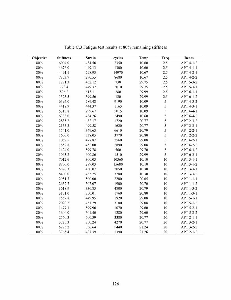
Table C.3 Fatigue test results at 80% remaining stiffness
Objective Stiffness Strain cycles Temp Freq Beam 80% 6004.0 434.56 2350 10.60 2.5 APT 4-1-2 80% 4676.0 449.13 1300 10.60 2.5 APT 4-1-1 80% 4491.1 298.93 14970 10.67 2.5 APT 4-2-1 80% 7353.7 290.55 8680 10.67 2.5 APT 4-2-2 80% 1271.3 452.12 730 29.75 2.5 APT 5-3-2 80% 778.4 449.32 2010 29.75 2.5 APT 5-3-1 80% 896.2 613.11 280 29.99 2.5 APT 6-1-1 80% 1525.5 599.56 120 29.99 2.5 APT 6-1-2 80% 6395.0 289.48 9190 10.09 5 APT 4-3-2 80% 4418.9 444.37 1165 10.09 5 APT 4-3-1 80% 5313.8 299.67 5015 10.09 5 APT 6-4-1 80% 6383.0 434.26 2490 10.60 5 APT 6-4-2 80% 2835.2 482.17 1720 20.77 5 APT 2-3-2 80% 2155.3 499.58 1620 20.77 5 APT 2-3-1 80% 1541.0 349.63 6610 20.79 5 APT 2-2-1 80% 1600.0 338.05 3770 20.80 5 APT 2-2-2 80% 1052.5 477.87 2560 29.08 5 APT 6-2-1 80% 1852.8 452.00 2890 29.08 5 APT 6-2-2 80% 1424.0 599.78 560 29.70 5 APT 6-3-2 80% 1063.2 600.86 1510 29.99 5 APT 6-3-1 80% 7012.6 300.03 10360 10.10 10 APT 3-1-1 80% 8800.0 289.03 15680 10.10 10 APT 3-1-2 80% 5820.3 450.07 2050 10.30 10 APT 3-3-1 80% 8400.0 433.25 3280 10.30 10 APT 3-3-2 80% 2951.7 500.00 2200 20.65 10 APT 1-1-1 80% 2632.7 507.07 1900 20.70 10 APT 1-1-2 80% 3618.9 336.83 4800 20.79 10 APT 1-3-2 80% 3171.0 350.01 1760 20.80 10 APT 1-3-1 80% 1557.8 449.95 1920 29.08 10 APT 5-1-1 80% 2020.2 451.29 3100 29.08 10 APT 5-1-2 80% 1477.1 599.96 1070 29.60 10 APT 5-2-1 80% 1640.0 601.40 1280 29.60 10 APT 5-2-2 80% 2560.3 500.39 3380 20.77 20 APT 2-1-1 80% 3725.3 350.24 4270 20.77 20 APT 3-2-1 80% 5275.2 336.64 5440 21.24 20 APT 3-2-2 80% 3765.4 481.39 1390 21.26 20 APT 2-1-2
126
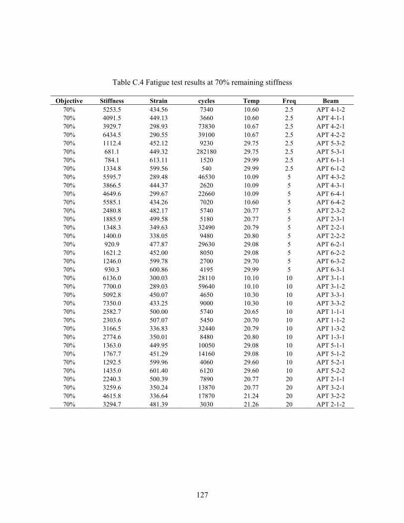
Table C.4 Fatigue test results at 70% remaining stiffness
Objective Stiffness Strain cycles Temp Freq Beam 70% 5253.5 434.56 7340 10.60 2.5 APT 4-1-2 70% 4091.5 449.13 3660 10.60 2.5 APT 4-1-1 70% 3929.7 298.93 73830 10.67 2.5 APT 4-2-1 70% 6434.5 290.55 39100 10.67 2.5 APT 4-2-2 70% 1112.4 452.12 9230 29.75 2.5 APT 5-3-2 70% 681.1 449.32 282180 29.75 2.5 APT 5-3-1 70% 784.1 613.11 1520 29.99 2.5 APT 6-1-1 70% 1334.8 599.56 540 29.99 2.5 APT 6-1-2 70% 5595.7 289.48 46530 10.09 5 APT 4-3-2 70% 3866.5 444.37 2620 10.09 5 APT 4-3-1 70% 4649.6 299.67 22660 10.09 5 APT 6-4-1 70% 5585.1 434.26 7020 10.60 5 APT 6-4-2 70% 2480.8 482.17 5740 20.77 5 APT 2-3-2 70% 1885.9 499.58 5180 20.77 5 APT 2-3-1 70% 1348.3 349.63 32490 20.79 5 APT 2-2-1 70% 1400.0 338.05 9480 20.80 5 APT 2-2-2 70% 920.9 477.87 29630 29.08 5 APT 6-2-1 70% 1621.2 452.00 8050 29.08 5 APT 6-2-2 70% 1246.0 599.78 2700 29.70 5 APT 6-3-2 70% 930.3 600.86 4195 29.99 5 APT 6-3-1 70% 6136.0 300.03 28110 10.10 10 APT 3-1-1 70% 7700.0 289.03 59640 10.10 10 APT 3-1-2 70% 5092.8 450.07 4650 10.30 10 APT 3-3-1 70% 7350.0 433.25 9000 10.30 10 APT 3-3-2 70% 2582.7 500.00 5740 20.65 10 APT 1-1-1 70% 2303.6 507.07 5450 20.70 10 APT 1-1-2 70% 3166.5 336.83 32440 20.79 10 APT 1-3-2 70% 2774.6 350.01 8480 20.80 10 APT 1-3-1 70% 1363.0 449.95 10050 29.08 10 APT 5-1-1 70% 1767.7 451.29 14160 29.08 10 APT 5-1-2 70% 1292.5 599.96 4060 29.60 10 APT 5-2-1 70% 1435.0 601.40 6120 29.60 10 APT 5-2-2 70% 2240.3 500.39 7890 20.77 20 APT 2-1-1 70% 3259.6 350.24 13870 20.77 20 APT 3-2-1 70% 4615.8 336.64 17870 21.24 20 APT 3-2-2 70% 3294.7 481.39 3030 21.26 20 APT 2-1-2
127
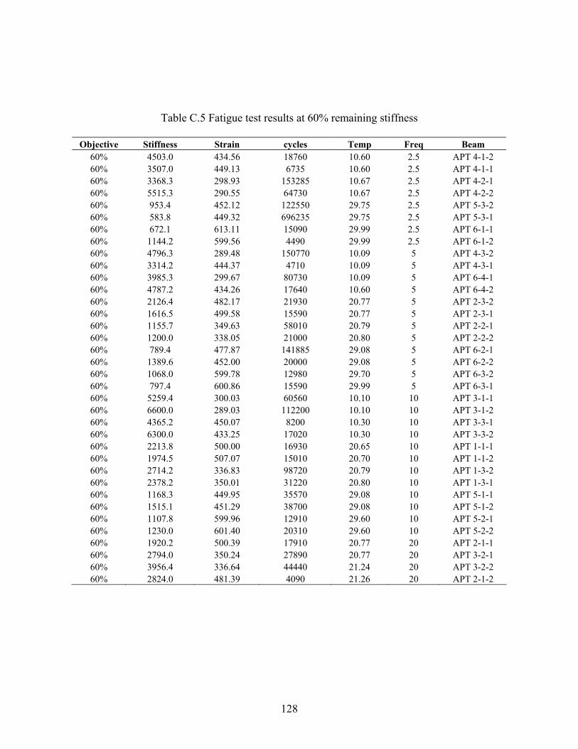
Table C.5 Fatigue test results at 60% remaining stiffness
Objective Stiffness Strain cycles Temp Freq Beam 60% 4503.0 434.56 18760 10.60 2.5 APT 4-1-2 60% 3507.0 449.13 6735 10.60 2.5 APT 4-1-1 60% 3368.3 298.93 153285 10.67 2.5 APT 4-2-1 60% 5515.3 290.55 64730 10.67 2.5 APT 4-2-2 60% 953.4 452.12 122550 29.75 2.5 APT 5-3-2 60% 583.8 449.32 696235 29.75 2.5 APT 5-3-1 60% 672.1 613.11 15090 29.99 2.5 APT 6-1-1 60% 1144.2 599.56 4490 29.99 2.5 APT 6-1-2 60% 4796.3 289.48 150770 10.09 5 APT 4-3-2 60% 3314.2 444.37 4710 10.09 5 APT 4-3-1 60% 3985.3 299.67 80730 10.09 5 APT 6-4-1 60% 4787.2 434.26 17640 10.60 5 APT 6-4-2 60% 2126.4 482.17 21930 20.77 5 APT 2-3-2 60% 1616.5 499.58 15590 20.77 5 APT 2-3-1 60% 1155.7 349.63 58010 20.79 5 APT 2-2-1 60% 1200.0 338.05 21000 20.80 5 APT 2-2-2 60% 789.4 477.87 141885 29.08 5 APT 6-2-1 60% 1389.6 452.00 20000 29.08 5 APT 6-2-2 60% 1068.0 599.78 12980 29.70 5 APT 6-3-2 60% 797.4 600.86 15590 29.99 5 APT 6-3-1 60% 5259.4 300.03 60560 10.10 10 APT 3-1-1 60% 6600.0 289.03 112200 10.10 10 APT 3-1-2 60% 4365.2 450.07 8200 10.30 10 APT 3-3-1 60% 6300.0 433.25 17020 10.30 10 APT 3-3-2 60% 2213.8 500.00 16930 20.65 10 APT 1-1-1 60% 1974.5 507.07 15010 20.70 10 APT 1-1-2 60% 2714.2 336.83 98720 20.79 10 APT 1-3-2 60% 2378.2 350.01 31220 20.80 10 APT 1-3-1 60% 1168.3 449.95 35570 29.08 10 APT 5-1-1 60% 1515.1 451.29 38700 29.08 10 APT 5-1-2 60% 1107.8 599.96 12910 29.60 10 APT 5-2-1 60% 1230.0 601.40 20310 29.60 10 APT 5-2-2 60% 1920.2 500.39 17910 20.77 20 APT 2-1-1 60% 2794.0 350.24 27890 20.77 20 APT 3-2-1 60% 3956.4 336.64 44440 21.24 20 APT 3-2-2 60% 2824.0 481.39 4090 21.26 20 APT 2-1-2
128
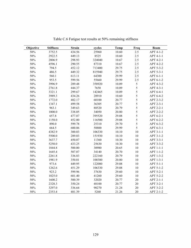
Table C.6 Fatigue test results at 50% remaining stiffness
Objective Stiffness Strain cycles Temp Freq Beam 50% 3752.5 434.56 25960 10.60 2.5 APT 4-1-2 50% 2922.5 449.13 8525 10.60 2.5 APT 4-1-1 50% 2806.9 298.93 324040 10.67 2.5 APT 4-2-1 50% 4596.1 290.55 87310 10.67 2.5 APT 4-2-2 50% 794.5 452.12 713400 29.75 2.5 APT 5-3-2 50% 486.5 449.32 815940 29.75 2.5 APT 5-3-1 50% 560.1 613.11 64300 29.99 2.5 APT 6-1-1 50% 953.5 599.56 55660 29.99 2.5 APT 6-1-2 50% 3996.9 289.48 358920 10.09 5 APT 4-3-2 50% 2761.8 444.37 7650 10.09 5 APT 4-3-1 50% 3321.1 299.67 142465 10.09 5 APT 6-4-1 50% 3989.3 434.26 28910 10.60 5 APT 6-4-2 50% 1772.0 482.17 60100 20.77 5 APT 2-3-2 50% 1347.1 499.58 36305 20.77 5 APT 2-3-1 50% 963.1 349.63 88520 20.79 5 APT 2-2-1 50% 1000.0 338.05 34050 20.80 5 APT 2-2-2 50% 657.8 477.87 395520 29.08 5 APT 6-2-1 50% 1158.0 452.00 116500 29.08 5 APT 6-2-2 50% 890.0 599.78 25310 29.70 5 APT 6-3-2 50% 664.5 600.86 58800 29.99 5 APT 6-3-1 50% 4382.9 300.03 106330 10.10 10 APT 3-1-1 50% 5500.0 289.03 151930 10.10 10 APT 3-1-2 50% 3637.7 450.07 11360 10.30 10 APT 3-3-1 50% 5250.0 433.25 25630 10.30 10 APT 3-3-2 50% 1844.8 500.00 30980 20.65 10 APT 1-1-1 50% 1645.4 507.07 34140 20.70 10 APT 1-1-2 50% 2261.8 336.83 222160 20.79 10 APT 1-3-2 50% 1981.9 350.01 100380 20.80 10 APT 1-3-1 50% 973.6 449.95 122080 29.08 10 APT 5-1-1 50% 1262.6 451.29 106330 29.08 10 APT 5-1-2 50% 923.2 599.96 37630 29.60 10 APT 5-2-1 50% 1025.0 601.40 41260 29.60 10 APT 5-2-2 50% 1600.2 500.39 32020 20.77 20 APT 2-1-1 50% 2328.3 350.24 48100 20.77 20 APT 3-2-1 50% 3297.0 336.64 90270 21.24 20 APT 3-2-2 50% 2353.4 481.39 5260 21.26 20 APT 2-1-2
129
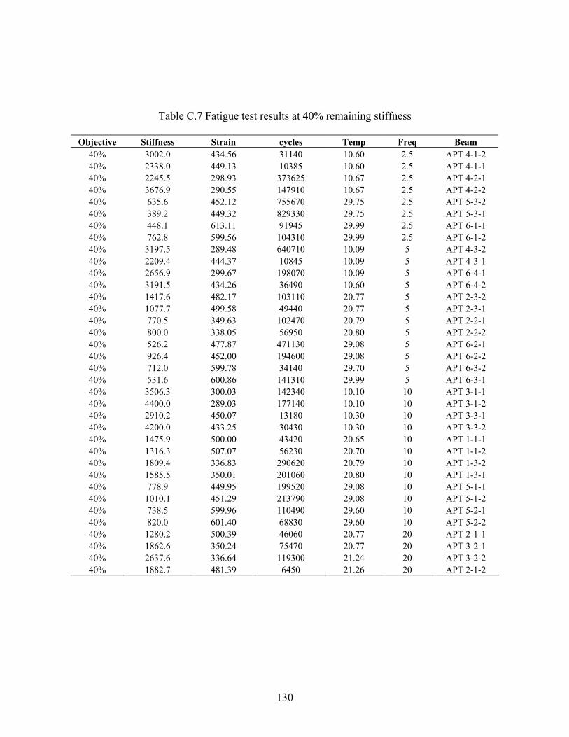
Table C.7 Fatigue test results at 40% remaining stiffness
Objective Stiffness Strain cycles Temp Freq Beam 40% 3002.0 434.56 31140 10.60 2.5 APT 4-1-2 40% 2338.0 449.13 10385 10.60 2.5 APT 4-1-1 40% 2245.5 298.93 373625 10.67 2.5 APT 4-2-1 40% 3676.9 290.55 147910 10.67 2.5 APT 4-2-2 40% 635.6 452.12 755670 29.75 2.5 APT 5-3-2 40% 389.2 449.32 829330 29.75 2.5 APT 5-3-1 40% 448.1 613.11 91945 29.99 2.5 APT 6-1-1 40% 762.8 599.56 104310 29.99 2.5 APT 6-1-2 40% 3197.5 289.48 640710 10.09 5 APT 4-3-2 40% 2209.4 444.37 10845 10.09 5 APT 4-3-1 40% 2656.9 299.67 198070 10.09 5 APT 6-4-1 40% 3191.5 434.26 36490 10.60 5 APT 6-4-2 40% 1417.6 482.17 103110 20.77 5 APT 2-3-2 40% 1077.7 499.58 49440 20.77 5 APT 2-3-1 40% 770.5 349.63 102470 20.79 5 APT 2-2-1 40% 800.0 338.05 56950 20.80 5 APT 2-2-2 40% 526.2 477.87 471130 29.08 5 APT 6-2-1 40% 926.4 452.00 194600 29.08 5 APT 6-2-2 40% 712.0 599.78 34140 29.70 5 APT 6-3-2 40% 531.6 600.86 141310 29.99 5 APT 6-3-1 40% 3506.3 300.03 142340 10.10 10 APT 3-1-1 40% 4400.0 289.03 177140 10.10 10 APT 3-1-2 40% 2910.2 450.07 13180 10.30 10 APT 3-3-1 40% 4200.0 433.25 30430 10.30 10 APT 3-3-2 40% 1475.9 500.00 43420 20.65 10 APT 1-1-1 40% 1316.3 507.07 56230 20.70 10 APT 1-1-2 40% 1809.4 336.83 290620 20.79 10 APT 1-3-2 40% 1585.5 350.01 201060 20.80 10 APT 1-3-1 40% 778.9 449.95 199520 29.08 10 APT 5-1-1 40% 1010.1 451.29 213790 29.08 10 APT 5-1-2 40% 738.5 599.96 110490 29.60 10 APT 5-2-1 40% 820.0 601.40 68830 29.60 10 APT 5-2-2 40% 1280.2 500.39 46060 20.77 20 APT 2-1-1 40% 1862.6 350.24 75470 20.77 20 APT 3-2-1 40% 2637.6 336.64 119300 21.24 20 APT 3-2-2 40% 1882.7 481.39 6450 21.26 20 APT 2-1-2
130
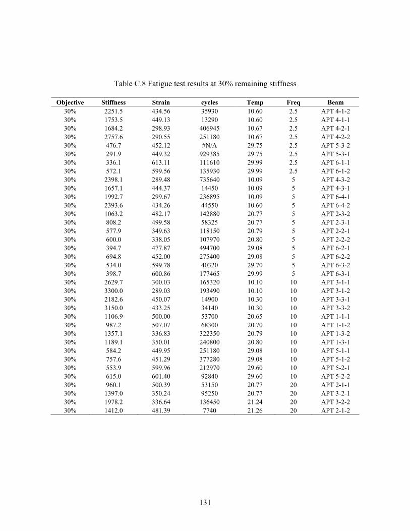
Table C.8 Fatigue test results at 30% remaining stiffness
Objective Stiffness Strain cycles Temp Freq Beam 30% 2251.5 434.56 35930 10.60 2.5 APT 4-1-2 30% 1753.5 449.13 13290 10.60 2.5 APT 4-1-1 30% 1684.2 298.93 406945 10.67 2.5 APT 4-2-1 30% 2757.6 290.55 251180 10.67 2.5 APT 4-2-2 30% 476.7 452.12 #N/A 29.75 2.5 APT 5-3-2 30% 291.9 449.32 929385 29.75 2.5 APT 5-3-1 30% 336.1 613.11 111610 29.99 2.5 APT 6-1-1 30% 572.1 599.56 135930 29.99 2.5 APT 6-1-2 30% 2398.1 289.48 735640 10.09 5 APT 4-3-2 30% 1657.1 444.37 14450 10.09 5 APT 4-3-1 30% 1992.7 299.67 236895 10.09 5 APT 6-4-1 30% 2393.6 434.26 44550 10.60 5 APT 6-4-2 30% 1063.2 482.17 142880 20.77 5 APT 2-3-2 30% 808.2 499.58 58325 20.77 5 APT 2-3-1 30% 577.9 349.63 118150 20.79 5 APT 2-2-1 30% 600.0 338.05 107970 20.80 5 APT 2-2-2 30% 394.7 477.87 494700 29.08 5 APT 6-2-1 30% 694.8 452.00 275400 29.08 5 APT 6-2-2 30% 534.0 599.78 40320 29.70 5 APT 6-3-2 30% 398.7 600.86 177465 29.99 5 APT 6-3-1 30% 2629.7 300.03 165320 10.10 10 APT 3-1-1 30% 3300.0 289.03 193490 10.10 10 APT 3-1-2 30% 2182.6 450.07 14900 10.30 10 APT 3-3-1 30% 3150.0 433.25 34140 10.30 10 APT 3-3-2 30% 1106.9 500.00 53700 20.65 10 APT 1-1-1 30% 987.2 507.07 68300 20.70 10 APT 1-1-2 30% 1357.1 336.83 322350 20.79 10 APT 1-3-2 30% 1189.1 350.01 240800 20.80 10 APT 1-3-1 30% 584.2 449.95 251180 29.08 10 APT 5-1-1 30% 757.6 451.29 377280 29.08 10 APT 5-1-2 30% 553.9 599.96 212970 29.60 10 APT 5-2-1 30% 615.0 601.40 92840 29.60 10 APT 5-2-2 30% 960.1 500.39 53150 20.77 20 APT 2-1-1 30% 1397.0 350.24 95250 20.77 20 APT 3-2-1 30% 1978.2 336.64 136450 21.24 20 APT 3-2-2 30% 1412.0 481.39 7740 21.26 20 APT 2-1-2
131

Table C.9 Fatigue test results at 20% remaining stiffness
Objective Stiffness Strain cycles Temp Freq Beam 20% 1501.0 434.56 52210 10.60 2.5 APT 4-1-2 20% 1169.0 449.13 21290 10.60 2.5 APT 4-1-1 20% 1122.8 298.93 452310 10.67 2.5 APT 4-2-1 20% 1838.4 290.55 382360 10.67 2.5 APT 4-2-2 20% 317.8 452.12 #N/A 29.75 2.5 APT 5-3-2 20% 194.6 449.32 #N/A 29.75 2.5 APT 5-3-1 20% 224.0 613.11 139030 29.99 2.5 APT 6-1-1 20% 381.4 599.56 189630 29.99 2.5 APT 6-1-2 20% 1598.8 289.48 836650 10.09 5 APT 4-3-2 20% 1104.7 444.37 20875 10.09 5 APT 4-3-1 20% 1328.4 299.67 263325 10.09 5 APT 6-4-1 20% 1595.7 434.26 67260 10.60 5 APT 6-4-2 20% 708.8 482.17 171130 20.77 5 APT 2-3-2 20% 538.8 499.58 67745 20.77 5 APT 2-3-1 20% 385.2 349.63 156080 20.79 5 APT 2-2-1 20% 400.0 338.05 169170 20.80 5 APT 2-2-2 20% 263.1 477.87 #N/A 29.08 5 APT 6-2-1 20% 463.2 452.00 #N/A 29.08 5 APT 6-2-2 20% 356.0 599.78 60720 29.70 5 APT 6-3-2 20% 265.8 600.86 213390 29.99 5 APT 6-3-1 20% 1753.1 300.03 181020 10.10 10 APT 3-1-1 20% 2200.0 289.03 218460 10.10 10 APT 3-1-2 20% 1455.1 450.07 17240 10.30 10 APT 3-3-1 20% 2100.0 433.25 38210 10.30 10 APT 3-3-2 20% 737.9 500.00 62930 20.65 10 APT 1-1-1 20% 658.2 507.07 77620 20.70 10 APT 1-1-2 20% 904.7 336.83 378730 20.79 10 APT 1-3-2 20% 792.7 350.01 289170 20.80 10 APT 1-3-1 20% 389.4 449.95 319580 29.08 10 APT 5-1-1 20% 505.0 451.29 624380 29.08 10 APT 5-1-2 20% 369.3 599.96 275290 29.60 10 APT 5-2-1 20% 410.0 601.40 113060 29.60 10 APT 5-2-2 20% 640.1 500.39 69150 20.77 20 APT 2-1-1 20% 931.3 350.24 107560 20.77 20 APT 3-2-1 20% 1318.8 336.64 162180 21.24 20 APT 3-2-2 20% 941.3 481.39 8580 21.26 20 APT 2-1-2
132

Appendix D: Sensitivity Analysis of the Model Parameters on the Predicted Fatigue
Life of Flexible Pavements
The model verification and validation process requires conducting a sensitivity
analysis and assessing the reasonability of the influence of the model parameters on the
predicted fatigue life of flexible pavements.
The approach adopted in this study requires running the distress prediction model for
different combinations of input parameters within the experienced inference space.
Figures D.1 through D.3 show the overall influence on pavement fatigue life of the
different model parameters.
Figure D.1 Plot showing the influence of damage ratio on the predicted number of load
applications
133
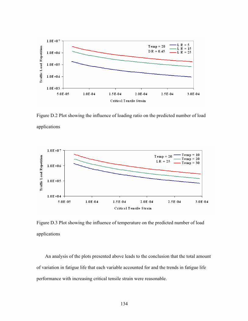
Figure D.2 Plot showing the influence of loading ratio on the predicted number of load
applications
Figure D.3 Plot showing the influence of temperature on the predicted number of load
applications
An analysis of the plots presented above leads to the conclusion that the total amount
of variation in fatigue life that each variable accounted for and the trends in fatigue life
performance with increasing critical tensile strain were reasonable.
134
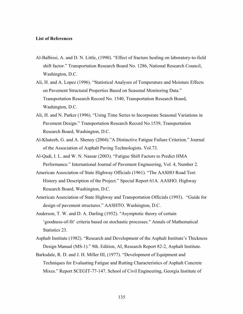
List of References
Al-Balbissi, A. and D. N. Little, (1990). “Effect of fracture healing on laboratory-to-field
shift factor.” Transportation Research Board No. 1286, National Research Council,
Washington, D.C.
Ali, H. and A. Lopez (1996). “Statistical Analyses of Temperature and Moisture Effects
on Pavement Structural Properties Based on Seasonal Monitoring Data.”
Transportation Research Record No. 1540, Transportation Research Board,
Washington, D.C.
Ali, H. and N. Parker (1996). “Using Time Series to Incorporate Seasonal Variations in
Pavement Design.” Transportation Research Record No.1539, Transportation
Research Board, Washington, D.C.
Al-Khateeb, G. and A. Shenoy (2004).”A Distinctive Fatigue Failure Criterion.” Journal
of the Association of Asphalt Paving Technologists. Vol.73.
Al-Qadi, I. L. and W. N. Nassar (2003). “Fatigue Shift Factors to Predict HMA
Performance.” International Journal of Pavement Engineering, Vol. 4, Number 2.
American Association of State Highway Officials (1961). “The AASHO Road Test:
History and Description of the Project.” Special Report 61A. AASHO. Highway
Research Board, Washington, D.C.
American Association of State Highway and Transportation Officials (1993). “Guide for
design of pavement structures.” AASHTO. Washington, D.C.
Anderson, T. W. and D. A. Darling (1952). "Asymptotic theory of certain
‘goodness-of-fit’ criteria based on stochastic processes." Annals of Mathematical
Statistics 23.
Asphalt Institute (1982). “Research and Development of the Asphalt Institute’s Thickness
Design Manual (MS-1).” 9th. Edition, AI, Research Report 82-2, Asphalt Institute.
Barksdale, R. D. and J. H. Miller III, (1977). “Development of Equipment and
Techniques for Evaluating Fatigue and Rutting Characteristics of Asphalt Concrete
Mixes.” Report SCEGIT-77-147. School of Civil Engineering, Georgia Institute of
135
Technology, Atlanta.
Bazin, P. and J.B.Saunier (1967). "Deformability, fatigue and healing properties of
asphalt mixes." Proceedings of the 2nd International Conference on the Structural
Design of Asphalt Pavements, Ann Arbor, Michigan.
Bonnaure, F., A. Gravois and J. Udron (1980). “A New Method for Predicting the
Fatigue Life of Bituminous Mixes.” Journal of the Association of Asphalt Paving
Technologists, Vol.49.
Bonnaure, F., A. H. J. J. Huibbers, and A. Booders (1982) "A Laboratory Investigation of
the Influence of Rest Periods on Fatigue Characteristics of Bituminous Mixes."
Journal of the Association of Asphalt Paving Technologists, Vol. 51.
Brown, S. F., J. M. Brunton, and P. S. Pell (1982). "The Development and
Implementation of Analytical Pavement Design for British Conditions." Proceedings,
Fifth International Conference on the Structural Design of Asphalt Pavements,
University of Michigan, Ann Arbor, Michigan.
Chatti, K., H. B. Kim, K. K. Yun, J.P. Mahoney and C. L. Monismith (1996). "Field
Investigation into Effects of Vehicle Speed and Tire Pressure on Asphalt Concrete
Pavement Strains." Transportation Research Record 1539, National Research
Council, Washington, D.C.
Chomton, G. and P. J. Valayer (1972). “Applied Rheology of Asphalt Mixes - Practical
Application.” Proceedings, Third International Conference on the Structural Design
of Asphalt Pavements, London.
Coetzee, N. F., W. Nokes, C. L. Monismith, J. Metcalf, and J. Mahoney (2000).
“Full-scale/Accelerated Pavement Testing: Current Status and Future Directions. A
TRB Millennium paper, A2B52: Task Force on Full-Scale/Accelerated Pavement
Testing.” Transportation Research Board, National Research Council, Washington,
D.C. Internet Document, http://gulliver.trb.org/publications/millennium/00046.pdf,
last accessed December 2006.
Cook, T. S. and F. Erdogan,. (1972). "Stresses in Bonded Materials with a Crack
Perpendicular to the Interface.” International Journal of Engineering Science, Vol. 10.
136
Cowher, K. (1975). “Cumulative Damage of Asphalt Materials under Repeated-Load
Indirect Tension.” Research Report Number 183-3. Center for Highway Research –
University of Texas at Austin.
Daniel, J. S., W. Bisirri and Y. R. Kim (2004). "Fatigue Evaluation of Asphalt Mixtures
Using Dissipated Energy and Viscoelastic Continuum Damage Approaches." Journal
of the Association of Asphalt Paving Technologists, Vol. 73.
Deacon, J. A. (1965). “Fatigue of Asphalt Concrete.” Ph.D. dissertation, University of
California. Berkeley.
Deacon, J. A., A. A. Tayebali, J. S. Coplantz, F. N. Finn, and C. L. Monismith (1994).
“Fatigue Response of Asphalt-Aggregate Mixes, Part III—Mix Design and Analysis.”
Strategic Highway Research Program Report No. SHRP-A-404, National Research
Council, Washington, D.C.
Deacon, J. A., J. S. Coplantz, A. A. Tayebali, and C. L. Monismith (1994). “Temperature
Considerations in Asphalt-Aggregate Mixture Analysis and Design.” Transportation
Research Record 1454, National Research Council, Washington, D.C.
De Beer, M. (1996). “Measurement of tyre/pavement interface tresses under moving
wheel loads.” International Journal of Vehicle Design. Special Issue on Vehicle-Road
and Vehicle-Bridge Interaction, Vol. 3, Nos. 1-4.
De la Roche, C., H. Odeon, J.P. Simoncelli, and A. Spernol (1994). “Study of the fatigue
of asphalt mixes using the circular test track of the laboratoire central des Ponts et
Chaussées in Nantes, France.” Transportation Research Record 1436, National
Research Council, Washington, D.C.
Drumm, E. C. and R. Meier (2003). “LTPP Data Analysis: Daily and Seasonal Variations
in Insitu Material Properties.” NCHRP Web Document 60, Transportation Research
Board, National Research Council, Washington, D.C.
Epps, J. and C. L. Monismith (1969). "Influence of mixture variables on the flexural
fatigue properties of asphalt concrete.” Journal of the Association of Asphalt Paving
Technologists, Vol.38.
137
Epps, J. and C. L. Monismith (1972). "Fatigue of asphalt concrete mixtures—A summary
of existing information." Fatigue of Compacted Bituminous Aggregate Mixtures,
Special Technical Publications 508, American Society for Testing and Materials.
Federal Highway Administration (2003). “Long-term pavement performance information
management system pavement performance database user guide.” FHWA, U.S.
Department of Transportation, Report No. FHWA-RD-03-088.
Federal Highway Administration (2003). “Distress Identification Manual for the
Long-Term Pavement Performance Program (Fourth Revised Edition).” FHWA, U.S.
Department of Transportation, Report No. FHWA-RD-03-031.
Federal Highway Administration (2007). “LTPP DataPave Online”, FHWA, available at
http://www.ltpp-products.com/, last accessed March 2007.
Gerritsen, A. H. and D. J. Jongeneel. (1988). "Fatigue Properties of Asphalt Mixes Under
Conditions of Very Low Loading Frequencies.” Journal of the Association of Asphalt
Paving Technologists, Vol. 57.
Ghuzlan, K.A.and S.H. Carpenter (2006)."Fatigue damage analysis in asphalt concrete
mixtures using the dissipated energy approach." Canadian Journal of Civil
Engineering, Vol. 33, Number 7.
Gramsammer, J. C., J. P. Kerzreho, and H. Odeon (1999). “The LCPC’s APT Facility.”
Proceedings, 9th International Conference on Accelerated Pavement Testing, Reno,
Nevada.
Hawai'i Asphalt Paving Industry (HAPI) (2007). "HAPI Asphalt Pavement Guide."
available at http://www.hawaiiasphalt.com/HAPI/index.htm, last accessed March
2007.
Harvey, J. T, L. du Plessis, F. Long, S. Shatnawi, C. Scheffy, B. Tsai, I. Guada, D. Hung,
N. Coetzee, M. Reimer, and C. L. Monismith (1996). “Initial CAL/APT Program:
Site Information, Test Pavement Construction, Pavement Materials Characterizations,
Initial CAL/APT Test Results, and Performance Estimates.” Pavement Research
Center, CAL/APT Program, Institute of Transportation Studies, University of
California, Berkeley.
138
Harvey, J. T., L. Louw, I. Guada, D. Hung, J. A. Prozzi, F. Long, and L. du Plessis.
(1999). “CAL/APT Program: Test Results from Accelerated Pavement Test on
Pavement Structure Containing Untreated Aggregate Base—Section 501RF.”
Pavement Research Center, CAL/APT Program, Institute of Transportation Studies,
University of California, Berkeley.
Hiller, J. E.and J. R. Roesler (2005). "Determination of Critical Concrete Pavement
Fatigue Damage Locations Using Influence Lines." Journal of Transportation
Engineering, Vol. 131, Issue 8.
Hsu, T. W. and K. H. Tseng (1996), “Effect of Rest Periods on Fatigue Response of
Asphalt Concrete Mixtures.” Journal of Transportation Engineering, ASCE. Vol. 122,
No. 4.
Huang, Y.H. (1993). Pavement Analysis and Design. Prentice Hall, NJ.
Hugo, F., B. F. McCullough, and B. van der Walt (1991). “Full-Scale Accelerated
Pavement Testing for the Texas State Department of Highways and Public
Transportation.” Transportation Research Record 1293, National Research Council,
Washington, D.C.
Hugo, F. and A. L. Epps (2004). “NCHRP Synthesis Practice 325: Significant Findings
from Full-Scale Accelerated Pavement Testing.” Transportation Research Board,
National Research Council, Washington, D.C.
Hveem, F. N. and R. M. Carmany (1948). “The Factors Underlying the Rational Design
of Pavements. Proceedings of the Highway Research Board, Vol. 28, Highway
Research Board, Washington, D.C.
Jiminez, R. Z. and B. M. Gallaway (1962). “Behavior of asphalt concrete diaphragms to
loading.” International Conference on the Structural Design of Asphalt Pavements,
Ann Arbor, Michigan.
Kallas, B. F. (1970). “Dynamic modulus of asphalt concrete in tension and compression.”
Journal of the Association of Asphalt Paving Technologists. Vol.39.
139
Kallas, B. F. and V. P. Puzinauskas (1972). “Flexural Fatigue Tests on Asphalt Paving
Mixtures.” Fatigue of Compacted Bituminous Aggregate Mixtures, Special Technical
Publications 508, American Society for Testing and Materials.
Kennedy, T. W. (1977). “Characterization of asphalt pavement material using the indirect
tensile test.” Journal of the Association of Asphalt Paving Technologists, Vol. 46.
Kim, B. and R. Roque (2006). “Evaluation of Healing Property of Asphalt Mixtures.”
Transportation Research Record 1970, Transportation Research Board, National
Research Council, Washington, D.C.
Long, F., J. T. Harvey, C. Scheffy, and C. L. Monismith (1996). “Prediction of Pavement
Fatigue for California Department of Transportation Accelerated Pavement Testing
Program: Drained and Undrained Test Sections.” Transportation Research Record
1540, National Research Council, Washington, D.C.
Majidzadeh, K., E. M. Kauffmann and D. V. Ramsamooj (1971). "Application of
Fracture Mechanics in the Analysis of Pavement Fatigue.” Journal of the Association
of Asphalt Paving Technologists, Vol. 40.
Majidzadeh, K., E. Kauffmann, and C. Saraf (1972). “Analysis of Fatigue of Paving
Mixtures from the Fracture Mechanics Viewpoint.” Fatigue of Compacted
Bituminous Aggregate Mixtures, Special Technical Publications 508, American
Society for Testing and Materials.
Majidzadeh, K., C. Buranrom, and M. Karakomzian.(1976). "Applications of fracture
mechanics for improved design of bituminous concrete." Report No.76-91, FHWA,
U.S. Dept. of Transportation.
McLean, D. B. (1974). “Permanent Deformation Characteristics of Asphalt Concrete.”
Ph.D. thesis, University of California, Berkeley.
Metcalf, J. B. (1996). “NCHRP Synthesis of Highway Practice 235: Application of
Full-Scale Accelerated Pavement Testing.” Transportation Research Board, National
Research Council, Washington, D.C.
140

Metcalf, J. B. (2005). “NCHRP Active Project 10-66: Predicting In-Service Performance
of Flexible Pavements from Accelerated Pavement Testing.” Transportation Research
Board, National Research Council, Washington, D.C.
Mirza, M. W. and M. W. Witczak (1995). “Development of a Global Aging System for
Short and Long Term Aging of Asphalt Cements.” Journal of the Association of
Asphalt Paving Technologists, Vol. 64.
Molenaar, A.A.A., J. Groenendijk and A.E. van Dommelen (1999). “ Development of
performance models from APT.” Proceedings, 9th International Conference on
Accelerated Pavement Testing, Reno, Nevada.
Monismith, C. L. (1966). “Asphalt Mixture Behavior in Repeated Flexure.” Report No.
TE 66-66, ITIE, to California Division of Highways, University of California.
Monismith, C. L. and Deacon, J. A. (1969). "Fatigue of asphalt paving mixtures."
Transportation Engineering Journal. ASCE 95(2).
Monismith, C. L. and Y. M. Salam (1973). "Distress Characteristics of Asphalt Concrete
Mixes.” Journal of the Association of Asphalt Paving Technologists, Vol.42.
Monismith, C. L., K. Inkabi, D. B. McLean, and C. R. Freeme (1977). “Design
Considerations for Asphalt Pavements.” Report No. TE 77-1, University of
California, Berkeley.
Monismith, C. L. (1981). "Fatigue characteristics of asphalt paving mixtures and their us
in pavement design.” Proceedings, 18th Paving Conference, University of New
Mecico, Albuquerque.
Moore, R. K. and T. W. Kennedy (1971). “Tensile Behavior of Subbase Materials Under
Repetitive Loading.” Research Report 98-12, Center for Highway Research,
University of Texas at Austin, Austin, TX,
Navarro, D. and T, W. Kennedy (1975). "Fatigue and Repeated-Load Elastic
Characteristics of In-service Asphalt-Treated Pavement.” Research Report No.183-2,
Center for Highway Research, the University of Texas at Austin.
141
NCHRP (2006). “Mechanistic-Empirical Guide for the Design of New and Rehabilitated
Pavement Structures”, National Cooperative Highway Research Program, Project
1-37A, available at www.trb.org/mepdg/guide.htm, last accessed December 2006.
Newcomb, D. E., G. Engstrom, D. A. Van Deusen, J. A. Siekmeier, and D. H. Timm.
(1999). “Minnesota Road Research Project: A Five-Year Review of
Accomplishments.” Proceedings, 9th International Conference on Accelerated
Pavement Testing, Reno, Nevada.
Nijboer, L. W. and Van der Poel, C. (1953). “A Study of Vibration Phenomena in
Asphaltic Road Constructions.” Proceedings of the Association of Asphalt Paving
Technologists, Vol. 22.
Paris, P. and F. Erdogan (1963). “A critical analysis of crack propagation laws.” Journal
of Basic Engineering, Transactions of the American Society of Mechanical
Engineers, Vol. 85.
Pell, P.S. (1962). “Fatigue characteristics of bitumen and bituminous mixes.”
International conference on the structural design of asphalt pavements, Ann Arbor,
Michigan.
Pell, P.S. (1967). “Fatigue of asphalt pavement mixes.” Proceedings, Second
International conference on the structural design of asphalt pavements, Ann Arbor,
University of Michigan.
Pell, P. S. and I. F. Taylor (1969). "Asphaltic Road Materials in Fatigue.” Journal of the
Association of Asphalt Paving Technologists, Vol. 38.
Pell, P. S. and S. F. Brown (1972). “The characteristics of materials for the design of
flexible pavement structures.” Proceedings, Third International Conference on the
Structural Design of Asphalt Pavements, London.
Pell, P. S. and K. E. Cooper (1975). "The effect of testing and mix variables on the
fatigue performance of bituminous materials." Journal of the Association of Asphalt
Paving Technologists, Vol. 44.
Porter, B. P. and T. W. Kennedy (1975). “Comparison of Fatigue Test Methods for
Asphaltic Materials.” Research Report 183-4, Center for Highway Research, the
142
University of Texas at Austin.
Pronk, A.C. and P.C. Hopman (1990). "Energy dissipation: the leading factor of fatigue.
In Highway Research: Sharing the Benefits." Proceedings of the Conference of the
United States Strategic Highway Research Program, London, UK.
Prozzi, J. A. and M. de Beer (1997), “Mechanistic determination of equivalent damage
factors for. multiple load and axle configurations”, Proceedings of the 8th
International Conference on Asphalt Pavements, Vol. 1, Seattle.
Prozzi, J. A. and S. M. Madanat (2000). “Using duration models to analyze experimental
pavement failure data.” Transportation Research Record 1699, Transportation
Research Board, National Research Council, Washington, D.C., 87–94.
Prozzi, J.A., M. Sánchez Silva, S. Caro Spinel (2005). Uso de Ensayos Acelerados para
Predecir el Comportamiento Real de carreteras. Proceedings, Congres
Ibero-Latinoamericano del Asfalto, San José, Cost Rica.
Prozzi, J.A. and R. Guo (2007). Reliability-Based Approach for Using LTPP and APT
Test Results for Estimating Fatigue Performance. Session 508, the 86th
Transportation Research Board Annual Meeting, National Research Council,
Washington D.C.
Raithby, K. D. and A. B. Sterling (1970). "Effect of Rest Periods on Fatigue Performance
of Hot-Rolled Asphalt under Reversed Axial Loading.” Association of Asphalt
Paving Technologists, Vol. 39.
Raithby, K. D. and A. B. Sterling (1972). “Some Effects of Loading History on the
Performance of Rolled Asphalt.” TRRL-LR 496, Crowthorne, England.
Raithby, K. D. and J. T. Ramshaw (1972). “Effects of secondary compaction on the
fatigue performance of a hot-rolled asphalt.” TRRL-LR 471, Crowthorne, England.
Salam, Y.M. (1971). “Characteristics of Deformation and Fracture of Asphalt Concrete.”
Ph.D. Dissertation, University of California, Berkeley.
Shell (1978). “Shell Pavement Design Manual-Asphalt Pavement and Overlays for Road
Traffic.” Shell International Petroleum, London.
143
Sherwood, J.A., X. Qi, P. Romero, K.D. Stuart, S. Naga, N.L. Thomas, and W. Mogawer.
(1999). “Full-scale pavement fatigue testing from FHWA superpave validation
study.” Proceedings, International conference on Accelerated Pavement Testing,
Reno, Nevada.
Sousa, J.B. (1986). “Dynamic Properties of Pavement Materials.” Ph.D. thesis,
University of California, Berkeley.
Strategic Highway Research Program (1994). “SHRP-LTPP General Pavement Studies:
Five-Year Report.” SHRP, National Research Council, Washington, D.C.
Stuart, K. D., W. S. Mogawer, and P. Romero (2002). "Validation of the superpave
asphalt binder fatigue cracking parameter using an Accelerated Loading Facility."
Rep. No. FHWA-RD-01-093, Federal Highway Administration, McLean, Va.
Sun, L. and W.R. Hudson (2005). “Probabilistic approaches for pavement fatigue
cracking prediction based on cumulative damage using Miner's law.” Journal of
Engineering Mechanics, Vol. 131, No 5.
Tangella, R., J. A. Deacon, and C. L. Monismith (1990). “Summary report of fatigue
response of asphalt mixtures.” Technical Memorandum No. M-UCB-A-003A-89-3M,
prepared for SHRP Project A-003A. Institute of Transportation Studies, University of
California, Berkeley.
Tayebali, A. A., G. M. Rowe, and J. B. Sousa (1992). "Fatigue response of
asphalt–aggregate mixtures." Journal of the Association of Asphalt Paving
Technologists, Vol. 61.
Tayebali, A. A., J. S. Coplantz, J.A. Deacon, F. N. Finn, and C. L. Monismith. (1994),
“Fatigue Response of Asphalt-Aggregate Mixtures.” Report No. SHRP-A-404,
Strategic Highway Research Program, National Research Council, Washington, D.C.
Theyse, H. L., M. De Beer, and F. C. Rust (1996). "Overviews of South African
Mechanistic Pavement Design Method." Transportation Research Record 1539,
Transportation Research Board, National Research Council, Washington, D.C.
144
Thompson, M. R.(1996). "Mechanistic-Empirical Flexible Pavement Design: An
Overview." Transportation Research Record 1539, Transportation Research Board,
National Research Council, Washington, D.C.
Tsai, B. W., Harvey, J. T., and Monismith, C. L. (2003). “The application of weibull
theory in asphalt concrete fatigue performance prediction.” Transportation Research
Board Annual Meeting Presentation, Washington, D.C.
Van Der Poel, C. (1954)."A General System Describing the Viscoelastic Properties of
Bitumens and its Relations to Routine Test Data." Journal of Applied Chemistry, Vol.
4.
Van Dijk, W., H. Moreaud, A. Quedeville and P.Uge (1972). “The Fatigue of Bitumen
and Bituminous Mixes.” Journal of the Association of Asphalt Paving Technologists,
Vol. 38.
Van Dijk, W. (1975). “Practical Fatigue Characterization of Bituminous Mixes.” Journal
of the Association of Asphalt Paving Technologists, Vol. 44.
Van Dijk, W. and W. Vesser (1977). ”The Energy Approach to Fatigue for. Pavement
Design.” Journal of the Association of Asphalt Paving Technologists, Vol.46.
Wang, F., R. F. Inman, R. B. Machemehl, Z. Zhang and C. M. Walton (2000). “Study of
Current Truck Configurations.” Tx-00/1862-2. Texas Department of Transportation,
Austin.
145

VITA
Runhua Guo was born in Jianshi, Hubei, China on November 5, 1975, the son of
Zhonghe Guo and Shifeng Yang. After completing his study at Enshi Senior High School
in 1993, he entered Tongji University in Shanghai. He earned the degree of Bachelor of
Engineering and Master of Engineering in civil engineering from Tongji University in
July 1997 and March 2000 respectively. In January 2002 he entered the transportation
group of the University of Texas at Austin. During the following years, he worked as a
graduate research assistant at the Center for Transportation Research of the University.
His primary research interests include Accelerated Pavement Testing (APT), pavement
performance modeling, integrated transportation infrastructure management and
pavement management systems, applications of probability and statistics in transportation
engineering, pavement materials and testing, and applications of Geographic information
system (GIS) in transportation engineering.
Permanent Address: #1 Guangrun road, Jianshi jibing kongzhi zhongxin, Hubei Province,
P.R.China 445300
This dissertation was typed by the author.
146