core mathematics at usma math/cmb-2014...... about the core mathematics ... mathematical skills and...

CORE MATHEMATICS

ACADEMIC YEAR 2014 – 2015

CORE MATHEMATICS AT USMA AY 14-15

CONTENTS: INTRODUCTION . . . . . . . . . . . . . . . . . . . . . . . . . . . . . . . . . . . . . . . . . . . . . . . . . . . . . . . 1 EDUCATIONAL PHILOSOPHY . . . . . . . . . . . . . . . . . . . . . . . . . . . . . . . . . . . . . . . . . . . 3 ADAPTIVE CURRICULUM . . . .. . . . . . . . . . . . . . . . . . . . . . . . . . . . . . . . . . . . . . . . . . . 4 SUPPORT OF USMA GOALS . . . .. . . . . . . . . . . . . . . . . . . . . . . . . . . . . . . . . . . . . . . . . 5 CORE MATH GOALS . . . . . . . . .. . . . . . . . . . . . . . . . . . . . . . . . . . . . . . . . . . . . . . . . . . . 7 THE ROLE OF TECHNOLOGY IN THE CORE MATH PROGRAM . . . . . .. . . . . 11 COURSE OBJECTIVES: MA100 . . . . . . . . . . . . . . . . . . . . . . . . . . . . . . . . . . . . . . . . . . . . . . . . . . . . . . . . . . . 13 MA103 . . . . . . . . . . . . . . . . . . . . . . . . . . . . . . . . . . . . . . . . . . . . . . . . . . . . . . . . . . . 16 MA104 . . . . . . . . . . . . . . . . . . . . . . . . . . . . . . . . . . . . . . . . . . . . . . . . . . . . . . . . . . . 19 MA205 . . . . . . . . . . . . . . . . . . . . . . . . . . . . . . . . . . . . . . . . . . . . . . . . . . . . . . . . . . . 23 MA206 . . . . . . . . . . . . . . . . . . . . . . . . . . . . . . . . . . . . . . . . . . . . . . . . . . . . . . . . . . . 25 MA153 . . . . . . . . . . . . . . . . . . . . . . . . . . . . . . . . . . . . . . . . . . . . . . . . . . . . . . . . . . . 27 MA255 . . . . . . . . . . . . . . . . . . . . . . . . . . . . . . . . . . . . . . . . . . . . . . . . . . . . . . . . . . . 30 MA364 . . . . . . . . . . . . . . . . . . . . . . . . . . . . . . . . . . . . . . . . . . . . . . . . . . . . . . . . . . . 33 INTERDISCIPLINARY GOAL………………………………………………. . . . . . . . . . . . 35 LIAISON PROFESSORS . . . . . . . . . . . . . . . . . . . . . . . . . . . . . . . . . . . . . . . . . . . . . . . . . . 38 MATHEMATICAL RECALL KNOWLEDGE . . . . . . . . . . . . . . . . . . . . . . . . . . . . . . . . . 39 REQUIRED SKILLS IN SCIENTIFIC COMPUTING . . . . . . . . . . . . . . . . . . . . . . . . . . . 43 REQUIRED MATHEMATICAL SKILLS FOR ENTERING CADETS . . . . . . . . . . . . . . 46 EXAMPLE FUNDAMENTAL CONCEPT EXAMS (FCEs) . . . . . . . . . . . . . . . . . . . . . 48 HISTORY OF THE DEPT OF MATHEMATICAL SCIENCES AT USMA . . . . . . . . . . 53

THIS PAGE INTENTIONALLY LEFT BLANK

1

CORE MATHEMATICS AT USMA AY 14-15

INTRODUCTION

This document is designed to inform USMA faculty in the Math/Science/Engineering (MSE) Departments, and interested others, about the core mathematics program. Inside you will learn what mathematical skills and concepts you can expect from your cadets as they progress from admission to the end of the core math sequence. You will see some of the philosophy and growth goals that we have adopted in order to develop a diverse group of high school graduates into college juniors who are prepared to succeed in an engineering stem or in higher-level disciplinary study. You will read about our new interdisciplinary goal and our Liaison Professor program. These programs aim to achieve a more integrated MSE experience for cadets by promoting coordination and collaboration between the Department of Mathematical Sciences and other academic departments. You will also learn the details of our program for identifying and reinforcing required mathematical skills for entering cadets. We have included a detailed summary of course objectives for each core math course for this academic year. As part of our educational philosophy, we recognize that mastering conceptual knowledge is a difficult process requiring periodic review, practice, and consolidation. Therefore, we recommend that courses which rely heavily on portions of this conceptual material identify those portions to the cadet at the beginning of the course, and then reinforce student understanding as appropriate. Also of special interest is the list of Mathematical Recall Knowledge. This is a modest list of basic facts designated by the MSE Committee that should be memorized by each cadet. Within the core math program, cadets periodically test their proficiency on this current and accumulated recall knowledge. For MSE courses that rely heavily on some subset of these recall skills, we again recommend that you identify these to your cadets at the beginning of the course, and then reinforce (and test) them as appropriate. Applied mathematics is the process of appropriately transforming one form into a more useful form in order to reveal additional insight. This can be as simple as transforming an array of numbers into a sum; a function into its derivative; or a computer network into a bipartite graph. A historian who can transform the data of secondary sources into information that reveals the interactions of an earlier society is an applied mathematician in disguise! It is essential that we provide our cadets an experience where they can appreciate and apply the power of transformations to solve real problems. Technologies are facilitating new transformations and have made other transformations obsolete. Hence, the teaching of mathematics at the undergraduate level is changing. While new technologies allow us to do innovative things today, experience strongly suggests that much of it will be only partly relevant, sometimes misleading, and occasionally wrong. We know that what we consider to be the fundamentals of mathematical knowledge change more slowly. Our role is to continually find the appropriate balance between technology and the fundamentals as mathematical pedagogy and content evolve. Thus we have identified a list of fundamental concepts both non-technology and technology related for each of our core courses.

2

We hope you find the information in this booklet useful. We welcome your feedback on how we can better coordinate our programs, and on what information we can include here in order to help you succeed as a teacher who uses the tools from core mathematics. The Department of Mathematical Sciences updates this document annually in coordination with the Math Science Goal Team. Please direct any comments to the former for inclusion in the next edition. STEVEN B. HORTON COL, Professor USMA Acting Head, Department of Mathematical Sciences DISTRIBUTION: Dean of the Academic Board Dept of Behavioral Sciences & Leadership Dept of Chemistry Dept of Civil and Mechanical Engineering Dept of Electrical Engineering & Computer Science Dept of Geography and Environmental Engineering

Dept of Mathematical Sciences Dept of Physics Dept of Social Sciences Dept of Systems Engineering

3

EDUCATIONAL PHILOSOPHY The Role of Core Mathematics Education at USMA

The mind is not a vessel to be filled but a flame to be kindled. -- Plutarch Core mathematics education at USMA includes both acquiring a body of knowledge and developing thought processes judged fundamental to a cadet's understanding of basic ideas in mathematics, science, and engineering. Equally important, this educational process in mathematics affords opportunities for cadets to progress in their development as life-long learners who are able to formulate intelligent questions and research answers independently and interactively. At the mechanical level, the core math program seeks to minimize memorization of a disjoint set of facts. The emphasis of the program is at the conceptual level, where the goal is for cadets to recognize relationships, similarities, and differences to help internalize the unifying framework of mathematical concepts. To enhance understanding of course objectives, major concepts are presented numerically, graphically, and symbolically. This helps cadets develop a visceral understanding that facilitates the use of these concepts in downstream science and engineering courses. Concepts are applied to representative problems from science, engineering, and the social sciences. These applications develop cadet experience in modeling and provide immediate motivation for developing a sound mathematical foundation for future studies. The core mathematics experience at USMA is not a terminal process wherein a requisite subset of mathematics knowledge is mastered. Rather, it is a vital step in an educational process that enables the cadet to acquire more sophisticated knowledge more independently. Cadet development dictates that we must provide the cadet time for experimentation, discovery, and reflection. Within this setting, review, practice, reinforcement, and consolidation of mathematical skills and concepts are necessary and appropriate, both within the core math program and in later science and engineering courses. Cadets completing the core math program will have developed a degree of proficiency in several modes of thought and habits of the mind. Cadets learn to reason deductively, inductively, algorithmically, by analogy, and with the ability to capture abstractions in models. The cadet who successfully completes the USMA core mathematics program will have a firm grasp of the fundamental thought processes underlying discrete and continuous processes, linear and nonlinear dynamics, and deterministic and stochastic processes. The cadet will possess a curious and experimental disposition, as well as the scholarship to formulate intelligent questions, to seek appropriate references, and to independently and interactively research answers. Most importantly, cadets will understand the role of applied mathematics – insight gained from transformations.

4

Adaptive Curriculum

The Department of Mathematical Sciences is committed to taking the lead in developing an effective mathematics curriculum that attempts to foresee the mathematical needs of tomorrow’s students. Our goal is to create a mathematics program that will enhance the mathematical maturity and problem solving skills of students. Technology has reversed the roles of calculus and modeling. Traditionally, calculus determined the core program and modeling was used to support the application aspect of the program. Tomorrow, modeling and inquiry will determine the program with calculus and other mathematics subjects supporting the modeling portion of the program. Placing an emphasis on both discrete and continuous modeling broadens the role of mathematics to include transforming real world problems into mathematical constructs, performing analysis, and interpreting results. Placing an emphasis on inquiry provides opportunities for student growth in terms of learning how to learn, becoming an exploratory learner, and taking responsibility for one’s own learning. Our approach is to provide students with a broad appreciation and practice of mathematics through modern ideas and applications. The program is designed to provide student experiences through important historical problems and noteworthy contemporary issues as well. The goal is for students to establish a foundation from which to address unanticipated problems of the future. Examples of problem domains that will be considered include: the fair distribution of resources among nations; scheduling transportation resources; network design; financial models; population models; statistical inference; motion in space; optimization models; position, location, and geometric models; accumulation models; growth and change models; long-term behavior of systems; algorithm analysis; numerical techniques; linear and non-linear systems; and heuristic techniques. Some problem domains will be revisited several times at more sophisticated levels throughout the core program as students develop into more competent problem solvers. Mathematics has the responsibility to develop a broad range of reasoning skills. The program will include contrasting approaches to problem solving such as: Continuous and Discrete; Linear and Non-linear; Deterministic and Stochastic; Deductive and Inductive; Exact and Approximate; Local and Global; Quantitative and Qualitative; and Science (what is) and Engineering (what can be). Exposure to the art of reasoning will come through the process of induction and deduction. We will create learning opportunities where students move from puzzling data to a suggested meaning (i.e., induction). Just as importantly, we will require students to move from the suggested meaning back to the data (i.e., deduction). This process of reasoning, along with other threads (e.g., approximation with error analysis, data analysis, and discovery), will run throughout the core program. Central to the entire program is the concept of problem solving in the modeling sense. This involves: (1) understanding the problem; (2) devising a plan to solve the problem; (3) carrying out the plan; and (4) looking back to examine the solution in the context of the original problem.

5

Disciplinary Depth: Graduates integrate and apply knowledge and methodological approaches gained through in-depth study of an academic discipline.

Critical Thinking and Creativity: Graduates think critically and creatively.

Communication: Graduates communicate effectively with all audiences.

Lifelong Learning: Graduates demonstrate the capability and desire to pursue progressive and continued intellectual development.

Science, Technology, Engineering, and Mathematics (STEM): Graduates apply STEM concepts and processes to solve complex problems.

SUPPORT OF USMA ACADEMIC GOALS The Role of Core Mathematics in the USMA Education

USMA Academic Program Goal: The USMA academic program is designed to accomplish the overarching USMA Academic Goal.

USMA Academic Goal

Graduates integrate knowledge and skills from a variety of disciplines to anticipate and respond appropriately to

opportunities and challenges in a changing world. Academic Program Goals: There are seven Academic Program Goals which support the above overarching USMA Academic Goal; of these, four are particularly pertinent to the Core Math Program, while key aspects of the Core Math curriculum support a fifth goal. The Core Math Program is uniquely designed to enable accomplishment of the Science, Technology, Engineering and Mathematics Goal. The Lifelong Learning, Communication, and Critical Thinking and Creativity goals are addressed in a successive and progressive manner by both the Core Mathematics program as well as other USMA programs. However, by virtue of its position at the beginning of the student’s academic program and the large amount of consecutive contact time, the Core Mathematics Program has a large responsibility for initial growth in these three areas. Recent efforts to integrate interdisciplinary pedagogical approaches in the Core Mathematics Program, in coordination with several other academic programs, contribute to the development of cadets’ ability to collaboratively engage challenges that span multiple disciplines, which is a sub-goal of Disciplinary Depth. Science, Technology, Engineering, and Mathematics (STEM) Academic Program Goal: The focus of the STEM Program Goal is on helping students develop various modes of thought in a rigorous manner, use a formal problem solving process to solve complex and ill-defined problems in science and engineering, develop scientific literacy sufficient to be able to understand and deal with the issues of society and our profession, and effectively apply technology to enhance their problem solving abilities. The Math-Science Goal Committee deems students to have demonstrated evidence of achieving these goals when they can do the following:

6

• Apply mathematics, science, and computing to model devices, systems, processes or behaviors. • Apply the scientific method. • Collect and analyze data in support of decision making. • Apply an engineering design process to create effective and adaptable solutions. • Understand and use information technology appropriately, adaptively, and securely. The two items in bold above are particularly pertinent to the Core Math Program. Lifelong Learning Academic Program Goal: The four semester contiguous core mathematics program plays an important role in transforming introductory college level students into independent learners prepared to begin study in their major discipline. The four-course connected curriculum provides a gradual transition from detailed to minimal direction. Each course provides the cadets with opportunities to take responsibility for their own learning. Embedded assessment indicators are used to track the role of the core mathematics curriculum in the continued intellectual development of our students. Communication Academic Program Goal: Throughout the four-semester core mathematics curriculum, cadets are expected to communicate their problem solving process both orally and in writing. They are introduced to the technical writing process and are evaluated according to the substance, organization, style, and correctness of their report. Each course also progressively develops cadets’ ability to read and interpret technical material through increased reliance on the textbook and independent learning exercises, and to actively listen and participate in class instruction. Critical Thinking and Creativity Academic Program Goal: Cadets completing the core mathematics program will have developed a degree of proficiency in several modes of thought and habits of mind. Cadets learn to solve complex problems through deductive and inductive reasoning, algorithmically, by analogy, and with the ability to capture abstractions in models. Interdisciplinary projects and activities are introduced throughout the core mathematics sequence developing our students’ ability to transfer learning across disciplines. The critical thinking skills gained solving complex, ill-defined problems in the core mathematics program are a vital element in creating graduates that can think and act creatively. Disciplinary Depth: The Core Mathematics Program facilitates the Disciplinary Depth goal in several ways. Much of the content is an integral part of the ABET accreditation process for several of the engineering related majors. The Core Mathematics Program provides students majoring in STEM disciplines as well as in Economics a broad overview of several fundamental tools and methods of inquiry. More generally, all cadets who complete the Core Mathematics Program get introduced to some of the basic limitations of mathematical modeling and reasoning processes. Additionally, all cadets participate in several interdisciplinary applications throughout the four-course sequence, and thus gain exposure to the importance of collaborative efforts that span multiple disciplines to make progress on some challenging and complex problems.

7

Core Mathematics Program Goals

Core Mathematics Program Goals: The goals of the Core Math program support the USMA Academic Program goals. The six primary goals of the Core Math program are provided and explained in further detail below.

Acquire a Body of Knowledge: Acquiring a body of knowledge is the foundation of the Core Math program. This body of knowledge includes the fundamental skills requisite to entry at USMA as well as the incorporation of new skills fundamental to the understanding of calculus and statistics. Incoming students are expected to be competent in algebra, trigonometry, and pre-calculus upon entry to USMA. Although many students have been introduced to calculus prior to entering USMA, the curriculum assumes that students possess no prior knowledge of calculus. Students will develop competence in the following skills and topic areas through the core math program: MA100

- Solve elementary algebra and geometry problems. - Analyze, manipulate, and solve equations and inequalities. - Recognize, sketch, and transform graphs and functions. - Define functions and draw their graphs. - Solve elementary inverse function problems. - Solve problems involving polynomial and rational functions. - Solve problems involving exponential and logarithmic problems. - Define trigonometric functions and solve problems involving trigonometric identities and - trigonometric equations. - Formulate mathematical models using the various functions described in the course.

MA103

- Model and solve problems using discrete systems and difference equations. - Apply matrix algebra to solve systems of equations. - Model and solve problems using continuous equations. - Use discrete and continuous models to make predictions. - Understand the concepts of limits and rates of change, and apply these concepts to assist in

understanding the long term behavior of mathematical models. - Understand when it is advantageous to use technology, especially when developing models,

exploring potential solutions, and iterating to find numerical solutions.

8

MA104

- Understand average and instantaneous rates of change - Understand the concept of the derivative and use this concept to model and solve problems. - Be able to take basic derivatives by hand (polynomials, trig, exponential, and logarithmic

functions). - Understand vectors and vector functions. - Understand partial derivatives, directional derivatives, and gradients and use these concepts to

model and solve problems. MA205

- Understand accumulation in one and more variables (Single and Multiple Variable Integration). - Be able to determine basic antiderivatives by hand (polynomials, trig, exponential and

logarithmic functions). - Use integrals to model and analyze simple physical problems. - Evaluate integrals and iterated integrals. - Be able to model real world problems using differential equations. - Use analytical, numerical, and graphical techniques to solve 1st and 2nd order differential

equations and systems of differential equations. MA206

- Understand the basic concepts of probability, statistics, and random variables. - Model applied problems using the fundamental probability distributions. - Make inferences about a population using Point Estimation, Interval Estimation, and Hypothesis

Testing. - Use Linear Regression to make predictions.

Communicate Effectively: Students learn mathematics only when they construct their own mathematical understanding. Successful problem solvers must be able to clearly articulate their problem solving process to others. Throughout the core math program, students will learn to:

- Actively listen to a presentation by a student of instructor and be able to synthesize information. - Read a mathematics textbook and either synthesize the material or frame appropariate questions

to clarify what they do not understand. - Articulate mathematical ideas in writing to include development of a mathematical model,

methods used to solve the model, and interpretation of the results. - Appropriately document all assignments according to the procedures in Documentation of Written

Work. - Articulate mathematical ideas orally in the form of board briefings, in class discussions, and

project presentations. Apply Technology: Technology can change the way students learn. Along with increased visualization, computer power has opened up a new world of applications and solution techniques. Our students can solve meaningful real-world problems by leveraging computer power appropriately. They will develop competence in the following skills through the core math program:

- Students will use both EXCEL and Mathematica to visualize, solve, analyze, and experiment with a myriad of mathematical functions (discrete, continuous, linear, non-linear, deterministic and stochastic). Specific skills are listed in the Required Skills for Scientific Computing section of this document.

- Students can interpret and correctly apply results obtained from EXCEL or Mathematica. - Students recognize the advantages and disadvantages of using technology, and can make wise

choices regarding when to use technology to assist with a problem. - Students are competent in using resources available to provide help in using technology, and are

capable of detecting errors and fixing faulty code. - Following the core sequence, we expect students to be confident and aggressive problem-solvers

who are able to use technology to leverage their ability to solve complex problems.

9

Build Competent and Confident Problem Solvers: The ultimate goal of the core mathematics program is the development of a competent and confident problem solver. Students need to apply mathematical reasoning and recognize relationships, similarities, and differences among mathematical concepts in order to solve problems. Given a problem, students will learn to:

- Identify information relevant to the problem and determine what they are trying to find. - Make reasonable and necessary assumptions to simplify the problem, and recognize the impact of

those assumptions. - Transform the problem into a mathematical model that can be solved using quantitative

techniques. - Choose appropriate techniques (computational, algorithmic, graphical, etc.) to solve the problem. - Interpret and apply the solution. - Perform sensitivity analysis to evaluate the impact of the assumptions.

Interdisciplinary Problem Solving: In today’s increasingly complex world, problems that leaders will face require the ability to consider a variety of perspectives. Mathematical analysis and results should not be accepted without understanding the social, economic, ethical and other concerns associated with the problem. The Core Math program seeks to expose cadets to problems with interdisciplinary scope. The goal is for cadets to consider what they have learned in other disciplines when faced with a problem requiring mathematical analysis. Additionally, cadets should appropriately apply mathematical concepts to support problems faced in other disciplines. Develop Habits of Mind: Learning is an inherently inefficient process. Learning how to teach oneself is a skill that requires maturity, discipline, and perseverance. In studying mathematics, students learn good scholarly habits for progressive intellectual development. The core mathematics program seeks to improve each cadet’s habits of mind in areas to include:

- Reasoning and Critical Thinking: Students can identify relevant information, ask questions to

clarify purpose or intent, make reasonable assumptions and recognize their affects, apply induction and deduction, develop a plan, and critique their own work.

- Creativity: Students can extend knowledge to new situations, draw upon previous experiences, develop illustrations to clarify concepts, establish connections between concepts, and take responsible risks.

- Work Ethic: Students strive for accuracy and precision, persist in the face of difficulty, attempt various methods without giving up, and remain focused on developing a solution strategy and implementing it.

- Thinking Interdependently: Students recognize potential contributions of team members, gather data from all sources, paraphrase another’s ideas, understand the diverse perspectives of others, and act responsibly in fulfilling group commitments.

- Life Long Learning and Curiosity: Students recognize the value of continuous learning, develop the ability to learn independently, learn to formulate questions to fill gaps between known and unknown, actively seek knowledge, and think about their own thinking (metacognition).

10

Core Mathematics Goals and Objectives G1: Students display effective habits of mind in their intellectual process. O1: Demonstrate curiosity toward learning new mathematics. O2: Reason and think critically through complex and challenging problems. O3: Demonstrate creativity and a willingness to take risks in their approach to solving new problems. O4: Display a sound work ethic, striving for accuracy and precision while maintaining strong resolve to complete problems in their entirety (e.g., persistence). O5: Think interdependently when working in groups. O6: Demonstrate the ability and motivation to learn new material without the help of the instructor. G2: Students demonstrate problem solving skills. O7: Transform problems into mathematical models that can be solved using quantitative techniques. O8: Select and apply appropriate mathematical methods as well as algorithmic and other computational techniques in the course of solving problems. O9: Interpret a mathematical solution to ensure that it makes sense in the context of the problem. G3: When appropriate, students apply technology to solve mathematical problems. O10: Use technology to visualize problems and, when appropriate, estimate solutions. O11: Use technology to explore possible solutions to mathematical problems and to conduct a sensitivity analysis. O12: Confidently use existing and new technologies to leverage their skills. G4: Students demonstrate an ability to communicate mathematics effectively. O13: Write to strengthen their understanding of mathematics and integrate their ideas. O14: Discuss their knowledge of mathematics to strengthen their understanding and integrate their ideas. O15: Understand and interpret written material (e.g., the textbook). O16: Listen actively to the instructor and student presentations. G5: Students demonstrate knowledge of mathematics. O17: Demonstrate competency of the fundamental skills required for entry into USMA. O18: Demonstrate competency of the fundamental skills required for each of the four core math courses.

O19: Demonstrate competency on major mathematical concepts for discrete math, linear algebra, probability and statistics, calculus, and differential equations covered in the core program.

G6: Students demonstrate an ability to consider problems from the perspective of multiple disciplines including mathematics. O20: Recognize the connections between disciplines when facing complex problems. O21: Consider the implications of issues from other disciplines when formulating and using mathematical models in problem solving. O22: Include analytical approaches and mathematical models to help the problem solving process when faced with a problem from another discipline.

11

The Role of Technology in the Core Math Program

“Mathematical sciences departments should employ technology in ways that foster teaching and learning, increase the students’ understanding of mathematical concepts, and prepare students for the use of technology in their careers or their graduate study. Where appropriate, courses offered by the department should integrate current technology. The availability of new technological tools and their pervasive use in the workplace have the potential for changing both the curriculum and the way that the mathematical sciences can and should be taught.” – Guidelines for Programs and Departments in Undergraduate Mathematical Sciences, The Mathematical Association of America, February 2003.

The Core Mathematics Program at USMA incorporates technology into the classroom throughout the four-semester sequence of courses to enhance student learning and understanding of mathematics, and to help produce graduates who are competent and confident at using and adapting to evolving technologies. Students use technology in the Core Math Program with the following purposes: (1) Exploration. Technology enhances students’ ability to explore mathematical ideas. For example, using technology, students can experiment by manipulating parameters of functions to see the effects, analyzing large data sets to look for patterns, fitting functions to data for use in predictive analysis, and developing new visual and graphical representations of relationships among variables. By removing time-consuming manual computations, students can focus on making conjectures, using technology to investigate and refine those conjectures, and better understand the underlying mathematics. (2) Visualization. Technology provides an easy way for students to visualize and gain understanding of previously intractable concepts. Graphs of higher dimensional functions, histograms or bar charts of large data sets, phase portraits of differential equations, and graphs of network systems are examples of visual tools that technology provides to the learner to help them gain better understanding. (3) Scientific Computing. The computing capability provided by technology frees students from unnecessarily tedious computations and allows students to solve complex problems that they cannot complete manually. The appropriate use of technology for scientific computing helps differentiate for students the problem solving skills that should be performed by humans (thinking, modeling, analyzing, developing algorithms) versus those that can be performed by machines (computing, iterating, executing algorithms, etc.) (4) Conceptual understanding. The use of technology can significantly contribute to students’ conceptual understanding of mathematics. Technology enables students to use multiple problem solving strategies – graphical, numerical, algebraic – on a given problem and compare/contrast results. Using technology for computational efforts frees up time for students to focus on understanding the mathematical ideas instead of just focusing on computational processes. The ability to explore and visualize gives them deeper insight and enables them to solve complex problems. In addition, the need to be “intelligent consumers of technology,” i.e. interpreting their results to determine if they make sense in the context of the problem, will help provide them with a better understanding of mathematics and problem solving.

12

Use of Technology in Core Courses Program directors and instructors of core mathematics courses will use the following guidelines when incorporating technology into a particular lesson: • Determine in advance the goal of using technology, and design the experience appropriately. • Focus on what the student needs from the technology and not on what the technology can do.

Students should not be overwhelmed with complicated code and requirements. Rather, they should be able to focus on the mathematics instead of being distracted by the difficulty of syntax or procedure.

• Be clear about expectations on the use of technology. If technology is used in class for a particular type of problem, students should be able to use it on an exam for that type of problem.

• Ensure the use of technology is pedagogy-based – use it when it enhances teaching/learning. The focus should not be on learning the specific technological tool but on the mathematics that students can learn as a result.

Since the appropriate application of technology is one of the goals of the core mathematics program, program directors will also assess the students’ ability to use technology. Part of this assessment will involve the students’ ability to perform specific tasks or skills; however, the following areas should also be considered:

1) Do students recognize when it is appropriate to use technology to aid in problem solving? 2) Can students look at the results obtained through technology and interpret them intelligently?

Can they reflect on the meaning of the results and evaluate whether the results make sense? 3) Can students use available resources, such as software-specific help menus, student guides, or on-

line search engines, to perform tasks while using technology, including tasks that may or may not have been demonstrated in the classroom or by an instructor? When students encounter errors in using technology, can they interpret the meaning of those errors and troubleshoot to fix them?

13

MA100 – Precalculus AY 14 – 15 Class of 2018 COURSE OBJECTIVES

MA100 prepares cadets with background deficiencies in algebra and trigonometry for the core mathematics program. The course develops fundamental skills in algebra, trigonometry, and functions through an introducation to mathematical modeling and problem solving, providing the mathematical foundation for an introductory calculus course. Note: Cadets taking MA100 will follow this course with MA101, Mathematical Mdoeling and Introduction to Calculus, and then MA104, Differential Calculua. Together, MA100 and MA101 count as MA103 is the 8TAP and cover all the course objectives and embedded skills in MA103. The course is broken down into four blocks of instruction. The block objectives are as follows: Block 1: Review of Fundamentals Objectives:

(1) Understand the properties of real numbers (e.g. integer, rational, irrational, negative), fractions, sets and intervals, and exponents and roots.

(2) Use basic properties of arithmetic operations to identify equivalent algebraic expressions and to re-express a given expression in various alternative forms to include:

- Expanding or simplifying expressions - Writing radical expressions as exponents and exponential expressions as radicals - Simplifying fractions and compound fractions.

(3) Explain what it meant to solve an equation or inequality, and do so for various types of problems.

(4) Use a Cartesian coordinate system to plot and identify points in a plane and to graph a function.

(5) Apply these skills in a wide variety of practical situations. Block 2: Functions Objectives:

(1) Understand the definition of a function and be able to evaluate a function at any value, numerical or symbolic.

(2) Be able to sketch the graph of a given function, to include piecewise functions, and be able to determine the function’s domain and range.

(3) Given the graph of a function 𝒚 = 𝒇(𝒙), know and understand the transformation that - Shifts it vertically and horizontally - Shrinks it vertically and horizontally - Reflects it about the x and y axis - Combines shifts, shrinks, and reflections.

(4) Understand the definitions of the following and be able to graph them: - Polynomial functions - Exponential functions - Logarithmic functions.

(5) Apply these skills in a wide variety of practical situations.

14

Block 3: Trigonometry Objectives:

(1) Understand the unit circle and the trigonometry of right triangles. (2) Understand the definition of and be able to graph trigonometric functions. (3) Understand the periodic properties of trigonometric functions and the transformations that

shift, stretch, and reflect trigonometric functions. (4) Understand the laws of sines and cosines. (5) Apply these skills in a wide variety of practical situations.

Block 4: Matrix Algebra Objectives:

(1) Understand and apply common vector and linear algebra concepts to include: - Vector addition and subtraction - Scalar multiplication with vectors and matrices - Matrix addition, subtractions, and multiplication - Matrix inverses - Elementary row operations to reduce a matrix.

(2) Formulate a model to represent certain situations with a vector, a matrix, or a system of linear equations.

15

Examples of Embedded Skills in MA100 which Support Course Objectives

1. Know the definition and understand the properties of real numbers, negative numbers,

fractions, sets and intervals, and absolute values. 2. Be able to write radical expressions using exponents and exponential expressions using

radicals. 3. Be able to use special product formulas to find products of (expand) and factor algebraic

expressions. 4. Be able to simplify, add, subtract, multiply and divide fractional expressions. 5. Know the definition of a linear equation, and be able to solve linear equations. 6. Given an equation, be able to solve for one variable in terms of others. 7. Be able to solve linear inequalities, nonlinear inequalities, inequalities involving a quotient,

and inequalities involving absolute values. 8. Be able to sketch a graph by plotting points, and find the x and y intercepts of the graph of

equations. 9. Understand the definition of function. 10. Be able to evaluate a function (to include piecewise functions) at any value, numeric or

symbolic. 11. Be able to find the domain and range of a function. 12. Understand average rate of change, how it is calculated and be able to apply the concept to

problem solving. 13. Given the graph of y = f(x), know and understand the transformation that shifts it vertically

and horizontally and be able to sketch it. 14. Be able to combine functions and form new ones through algebraic operations on functions. 15. Be able to determine the end behavior of polynomials. 16. Be able to define complex numbers. 17. Understand the definition of exponential and logarithmic functions. 18. Understand the definition of the natural logarithm and its properties and be able to evaluate

them. 19. Given a situation for circular motion, be able to find linear and angular speed. 20. Understand the definition of trigonometric functions. 21. Be able to express one trigonometric function in terms of another. 22. Be able to “solve a triangle” by determining all three angles and the lengths of all three sides. 23. Know the Law of Sines and Cosines. 24. Be able to graph trigonometric functions and their transformations. 25. Be able to use the substitution, elimination, and graphical methods to solve both linear and

nonlinear systems of equations. 26. Be able to determine the number of solutions of a linear system in two variables. 27. Understand the definition of vectors, what they represent, their graphical representation, and

their proper mathematical notation. 28. Be able to find the horizontal and vertical components of vectors. 29. Compute the dot (scalar) product of two vectors. 30. Solve systems of linear equations graphically and by substitution. 31. Solve systems of linear equations in several variables. 32. Understand the 3 possible number of solutions that a system of equations can have. For a

linear system of equations with 2 variables, understand what the solutions mean graphically. 33. Use elementary row operations to solve a linear system of equations. 34. Find sums, differences, and scalar products of matrices. 35. Be able to compute the product of matrices (perform matrix multiplication). 36. Write a linear system as a matrix equation. 37. Understand how the inverse of a matrix can be used in mathematical operations.

16

MA103 – Mathematical Modeling and Introduction to Calculus

AY 14-15 - Class of 2018 COURSE OBJECTIVES

MA103 is the first course of the mathematics core curriculum. It emphasizes applied mathematics through modeling and using effective problem solving strategies and modeling theory to solve complex and often, ill-defined problems. The course exercises mathematical concepts while nurturing creativity, critical thinking, and learning through activities performed in disciplinary, interdisciplinary, and multidisciplinary settings. Special emphasis is placed on introducing calculus using continuous and discrete mathematics through applied settings. The course exploits a variety of technological tools to develop numerical, graphical, and analytical solutions that enhance understanding. The course is broken down into five blocks of instruction, all focusing on connections to calculus. The block objectives are as follows: Block 1: Modeling with Discrete Dynamical Systems (Discrete Differential Equations) Objectives:

(1) Transform situations involving change at discrete intervals into mathematical models. (2) Solve a discrete dynamical system (DDS) numerically (through iteration), graphically, and

analytically (for linear cases). (3) Interpret the results of solving a DDS for a given problem.

Block 2: Introduction to Vectors and Matrices Objectives:

(1) Develop a base of knowledge of certain mathematical skills and concepts to allow for success in future math/science/engineering (MSE) courses at USMA.

(2) Understand and apply common vector and linear algebra concepts to include: a. Vector addition and subtraction b. Scalar multiplication of a vector and matrix c. Matrix multiplication d. Inverses e. Elementary row operations

(3) Solve a system of equations manually using linear algebra techniques. (4) Solve a system of equations graphically (for linear cases).

Block 3: Modeling with Matrices and Systems of Recursion Equations Objectives:

(1) Transform a situation into a mathematical model using a system of linear equations. (2) Solve a system of equations using technology. (3) Solve a system of equations analytically (for linear cases). (4) Evaluate and interpret the results of solving a system of recursion equations.

Block 4: Introduction to Continuous Functions Objectives:

(1) Understand common characteristics of continuous functions. (2) Explain the concepts of average and instantaneous rate of change as applicable to the

definition of the derivative. (3) Understand the graphical and algebraic interpretations of the derivative. (4) Determine and evaluate the derivative of functions using the properties of the derivative as

well as applying basic differentiation rules. Block 5: Modeling with Continuous Functions Objectives:

(1) Distinguish common families of functions (linear, exponential, power, and trigonometric), their properties, and how their parameters impact their shape.

(2) Transform a specified data set into a model using an appropriate continuous function. (3) Evaluate and interpret the results of solving a continuous model.

17


1. Given an initial condition, iterate a difference equation to find the value of interest in a sequence generated by the underlying recursion equation.

2. Determine equilibrium values for recursion equations algebraically, numerically, and graphically. 3. Determine the long term behavior of a discrete dynamical system using its analytic solution. 4. Determine an analytic solution for homogeneous and non-homogeneous linear Discrete

Dynamical Systems. 5. Algebraically verify an analytic solution to an initial value problem. 6. Find the sum and the difference of two vectors. 7. Multiply vectors by a scalar or a matrix. 8. Determine the dot product of two vectors. 9. Multiply a matrix by a scalar, matrix, or vector. 10. Solve (by hand) systems of equations (2x2) using substitution, row reduction, and the inverse of a

matrix. 11. Use technology to solve systems of equations of virtually any size using row reduction or the

inverse matrix method. 12. Understand the graphical interpretation of an eigenvector and eigenvalue and how to compute

each for a 2 x 2 matrix. 13. Using eigenvalues, eigenvectors, and vector decomposition, develop closed form solutions to

initial value problems involving systems of linear equations. 14. Using the definition of a function, determine which relationships are functions and which are not. 15. Describe the four different representations of functions. 16. Determine the limit of a function using graphic and numeric means. 17. Determine if a function is continuous, both at a point and on an interval. 18. Compute average rates of change to include slopes of secant lines and approximate instantaneous

rates of change by exploring the limits of the slopes of secant lines as well as calculating derivatives.

19. Know how parameters affect the shape of linear, exponential, power, and trigonometric functions; using one of these functions, evaluate a model’s utility and make comparisons by computing its sum of squared errors (SSE) and its coefficient of determination (r2).

20. Understand the graphical, algebraic and physical interpretations of the derivative. 21. Know, understand and apply the definition of the derivative. 22. Apply the definition of the derivative to find derivatives of functions. 23. Use the concepts of rates of change and derivatives to characterize the stability of the equilibrium

values of non-linear difference equations. 24. Understand the similarities and differences between first-order difference equations and first

order differential equations.

18

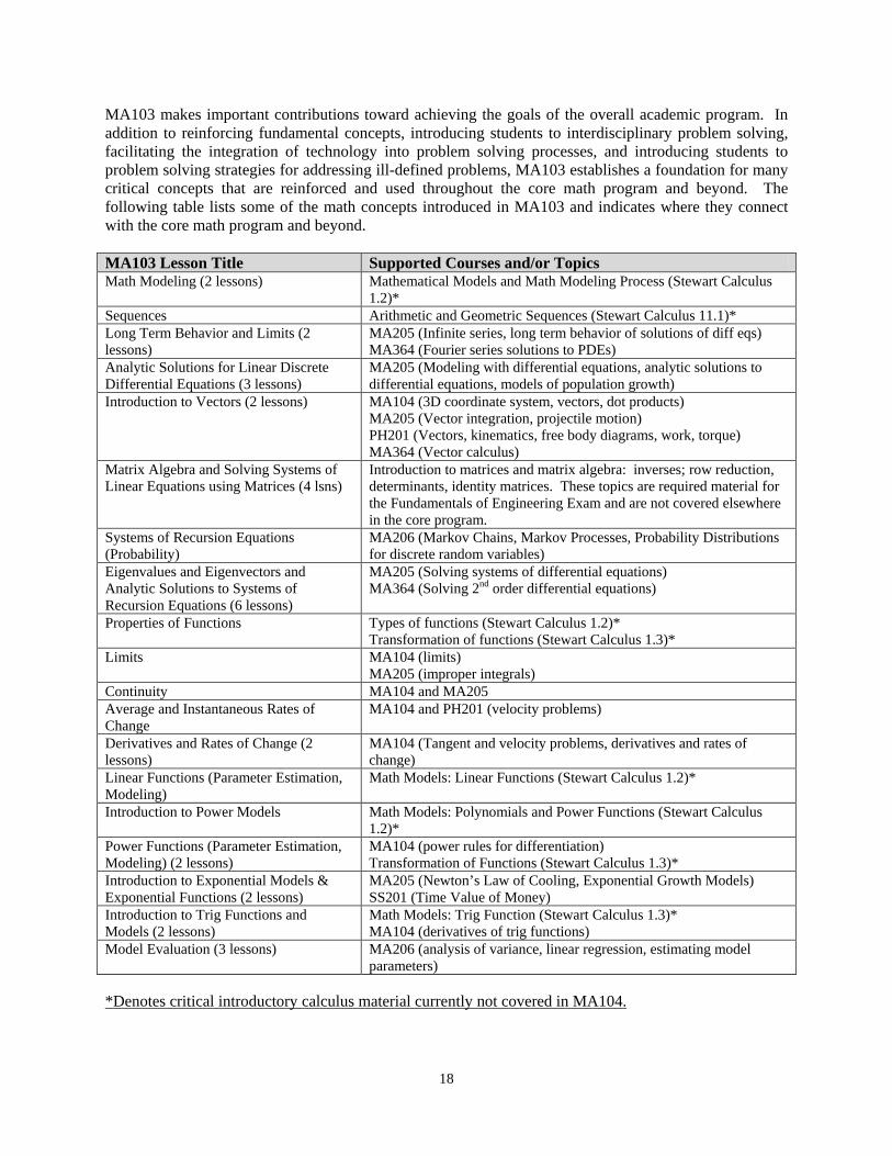
MA103 makes important contributions toward achieving the goals of the overall academic program. In addition to reinforcing fundamental concepts, introducing students to interdisciplinary problem solving, facilitating the integration of technology into problem solving processes, and introducing students to problem solving strategies for addressing ill-defined problems, MA103 establishes a foundation for many critical concepts that are reinforced and used throughout the core math program and beyond. The following table lists some of the math concepts introduced in MA103 and indicates where they connect with the core math program and beyond. MA103 Lesson Title Supported Courses and/or Topics Math Modeling (2 lessons) Mathematical Models and Math Modeling Process (Stewart Calculus

1.2)* Sequences Arithmetic and Geometric Sequences (Stewart Calculus 11.1)* Long Term Behavior and Limits (2 lessons)

MA205 (Infinite series, long term behavior of solutions of diff eqs) MA364 (Fourier series solutions to PDEs)

Analytic Solutions for Linear Discrete Differential Equations (3 lessons)

MA205 (Modeling with differential equations, analytic solutions to differential equations, models of population growth)

Introduction to Vectors (2 lessons) MA104 (3D coordinate system, vectors, dot products) MA205 (Vector integration, projectile motion) PH201 (Vectors, kinematics, free body diagrams, work, torque) MA364 (Vector calculus)

Matrix Algebra and Solving Systems of Linear Equations using Matrices (4 lsns)

Introduction to matrices and matrix algebra: inverses; row reduction, determinants, identity matrices. These topics are required material for the Fundamentals of Engineering Exam and are not covered elsewhere in the core program.

Systems of Recursion Equations (Probability)

MA206 (Markov Chains, Markov Processes, Probability Distributions for discrete random variables)

Eigenvalues and Eigenvectors and Analytic Solutions to Systems of Recursion Equations (6 lessons)

MA205 (Solving systems of differential equations) MA364 (Solving 2nd order differential equations)

Properties of Functions Types of functions (Stewart Calculus 1.2)* Transformation of functions (Stewart Calculus 1.3)*

Limits MA104 (limits) MA205 (improper integrals)

Continuity MA104 and MA205 Average and Instantaneous Rates of Change

MA104 and PH201 (velocity problems)

Derivatives and Rates of Change (2 lessons)

MA104 (Tangent and velocity problems, derivatives and rates of change)

Linear Functions (Parameter Estimation, Modeling)

Math Models: Linear Functions (Stewart Calculus 1.2)*

Introduction to Power Models Math Models: Polynomials and Power Functions (Stewart Calculus 1.2)*

Power Functions (Parameter Estimation, Modeling) (2 lessons)

MA104 (power rules for differentiation) Transformation of Functions (Stewart Calculus 1.3)*

Introduction to Exponential Models & Exponential Functions (2 lessons)

MA205 (Newton’s Law of Cooling, Exponential Growth Models) SS201 (Time Value of Money)

Introduction to Trig Functions and Models (2 lessons)

Math Models: Trig Function (Stewart Calculus 1.3)* MA104 (derivatives of trig functions)

Model Evaluation (3 lessons) MA206 (analysis of variance, linear regression, estimating model parameters)

*Denotes critical introductory calculus material currently not covered in MA104.

19

MA104 - CALCULUS I AY 14-15 - Class of 2018 COURSE OBJECTIVES

MA104 is the second semester of the mathematics core curriculum capitalizing on MA03’s introduction to vectors and calculus. This Differential Calculus course emphasizes the conceptual understanding of single and multivariable differentiation using modeling and problem solving techniques. Applications of the derivative such as optimization, rates of change in one and several variables, motion in space, and intersection/collisions are used to motivate the study of calculus. The course provides the basic mathematical foundation for further studies in mathematics, the physical sciences, the social sciences, and engineering. The course is broken down into five blocks of instruction focusing on differential and vector calculus. The objectives for each block are as follows: Block 1: Single Variable Differentiation Objectives:

(1) Recall, understand and be able to use mathematics from high school and previous math classes to include the definition of a function and its inverse as well as transcendental (exponential, logarithmic and trigonometric) functions.

(2) Understand the relationship and differences between average rate of change and instantaneous rate of change within the context of graphic, numeric, and algebraic representations.

(3) Determine and evaluate the derivative of functions using the properties of the derivative as well as applying differentiation rules.

(4) Find the derivatives of implicitly defined functions. (5) Calculate and interpret the antiderivative of a polynomial function with regards to

rectilinear motion.

Block 2: Applications of the Single Variable Derivative Objectives:

(1) Model and solve problems in which quantities grow or decay at a rate proportional to their size.

(2) Model and solve problems using rates of change, as well as related rates of change. (3) Approximate propagated error using single variable differentials. (4) Determine the local minima/maxima of a function and justify them with an appropriate

test. (5) Determine the absolute minimum/maximum of a function using the Closed Interval

Method. (6) Model and solve single variable optimization problems.

Block 3: Vector Functions and Geometry of Space Objectives:

(1) Develop parametric equations and understand how to use them in modeling problems.

20

(2) Understand the graphical and physical interpretation of vector functions and their derivatives.

(3) Calculate and interpret the dot product. (4) Calculate and interpret the cross product. (5) Develop and interpret mathematical models used to depict scenarios involving lines and

planes in space. (6) Differentiate vector functions and understand the corresponding graphical and physical

interpretation of the resulting derivatives. (7) Utilize vector functions to model and analyze the two-dimensional motion of an object or

the three-dimensional relative proximity of two objects moving through space.

Block 4: Multivariable Differentiation Objectives:

(1) Understand the graphical, numerical, and algebraic interpretations of functions of two or more variables.

(2) Calculate and interpret partial derivatives for a multivariable function. (3) Approximate propagated error using multivariable differentiation. (4) Calculate and interpret directional derivatives for a multivariable function. (5) Calculate and interpret the gradient vector for a multivariable function. (6) Produce a gradient vector field and use it to estimate the location of the critical points for

a multivariable function.

Block 5: Multivariable Optimization Objectives:

(1) Determine the local minima/maxima of a function of two variables and justify them with an appropriate test.

(2) Determine the absolute minima/maxima of a function of two variables on a closed and bounded set.

(3) Model and solve problems involving the optimization of a function of two variables. (4) Understand the geometry of a constrained problem and solve constrained multivariable

optimization problems using the Method of Lagrange Multipliers. (5) Use multivariable calculus and least squares to estimate the parameters of a polynomial

function which best fits a set of data.

21

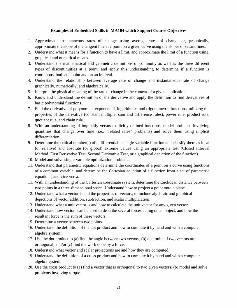
Examples of Embedded Skills in MA104 which Support Course Objectives 1. Approximate instantaneous rates of change using average rates of change or, graphically,

approximate the slope of the tangent line at a point on a given curve using the slopes of secant lines. 2. Understand what it means for a function to have a limit, and approximate the limit of a function using

graphical and numerical means. 3. Understand the mathematical and geometric definitions of continuity as well as the three different

types of discontinuities at a point, and apply this understanding to determine if a function is continuous, both at a point and on an interval.

4. Understand the relationship between average rate of change and instantaneous rate of change graphically, numerically, and algebraically.

5. Interpret the physical meaning of the rate of change in the context of a given application. 6. Know and understand the definition of the derivative and apply the definition to find derivatives of

basic polynomial functions. 7. Find the derivative of polynomial, exponential, logarithmic, and trigonometric functions, utilizing the

properties of the derivative (constant multiple, sum and difference rules), power rule, product rule, quotient rule, and chain rule.

8. With an understanding of implicitly versus explicitly defined functions, model problems involving quantities that change over time (i.e., “related rates” problems) and solve them using implicit differentiation.

9. Determine the critical number(s) of a differentiable single-variable function and classify them as local (or relative) and absolute (or global) extreme values using an appropriate test (Closed Interval Method, First Derivative Test, Second Derivative Test, or a graphical depiction of the function).

10. Model and solve single-variable optimization problems. 11. Understand that parametric equations determine the coordinates of a point on a curve using functions

of a common variable, and determine the Cartesian equation of a function from a set of parametric equations, and vice-versa.

11. With an understanding of the Cartesian coordinate system, determine the Euclidean distance between two points in a three-dimensional space. Understand how to project a point onto a plane.

12. Understand what a vector is and the properties of vectors, to include algebraic and graphical depictions of vector addition, subtraction, and scalar multiplication.

13. Understand what a unit vector is and how to calculate the unit vector for any given vector. 14. Understand how vectors can be used to describe several forces acting on an object, and how the

resultant force is the sum of these vectors. 15. Determine a vector between two points. 16. Understand the definition of the dot product and how to compute it by hand and with a computer

algebra system. 17. Use the dot product to (a) find the angle between two vectors, (b) determine if two vectors are

orthogonal, and/or (c) find the work done by a force. 18. Understand what vector and scalar projections are and how they are computed. 19. Understand the definition of a cross product and how to compute it by hand and with a computer

algebra system. 20. Use the cross product to (a) find a vector that is orthogonal to two given vectors, (b) model and solve

problems involving torque.

22

21. Be able to express the following in three-dimensional space: (a) a line using a point and a vector; (b) a line in space using a vector equation and a set of parametric equations; (c) vector and scalar equations of a plane in space using vectors; (d) an equation of a plane in space given either a point on the plane and a vector normal to the plane, or three points on the plane that do not lie on the same line; (e) the distance from a point to a given plane.

22. Understand the definition of a vector function and be able to find the domain of a vector function. 23. Understand how to calculate rates of change for vector functions and understand the physical

interpretation of the derivative of a vector function, to include the relationship between the position, velocity, and acceleration vectors for an object’s motion in space.

24. Be able to use the parametric equations of motion in order to solve projectile motion problems, to include (a) finding the velocity and acceleration vectors when given the position vector and an initial condition; (b) determining if the paths of two objects intersect given parametric equations modeling the paths of the objects in space; and (c) determining whether two objects collide, given parametric equations modeling the paths of the objects in space.

27. Given a function of two variables, determine the domain of the function. 28. Develop a general understanding of the use and meaning of level curves and level surfaces to

represent functions of two and three variables, respectively. 29. Understand the definition of a partial derivative and describe geometrically what a partial derivative

is for a function of two variables. 30. Approximate the partial derivative of a function of two variables at a point using average rates of

change. 31. Given a function of several variables, calculate the partial derivatives. 32. Understand what a directional derivative is in terms of a rate of change and, given a function 𝑓 of two

variables, find the directional derivative of 𝑓 at a given point in any direction. 33. Understand that the gradient vector gives the direction of the greatest increase in functional value at a

given point for a differentiable function and, given a function of two variables, find the gradient vector at a specified point.

34. Find the vector that is normal to the level curve𝑓(𝑥) = 𝑐 at a specified point. 35. Understand that the magnitude of the gradient vector gives the maximum rate of change of

differentiable function at a given point and how, geometrically, the gradient vector is related to level curves.

36. Given the surface 𝑧=(𝑥,𝑦), defined by a function which has continuous partial derivatives over some region 𝑹, examine the level curves for possible maximum or minimum values.

37. Determine the critical number(s) of a differentiable multivariate function of two variables, 𝑓(𝑥,𝑦), and classify them as local (or relative) and absolute (or global) extreme values using an appropriate test (Closed Interval Method, Second Derivatives Test, or a graphical depiction of the surface).

38. Model and solve simply constrained multivariable optimization problems for functions of two variables.

39. Solve optimization problems for functions of several variables subject to a single constraint using the Method of Lagrange Multipliers.

23

MA205 - CALCULUS II AY 14-15 – Class of 2017 COURSE OBJECTIVES

MA205 is the third semester of the mathematics core curriculum. This course provides a foundation for the continued study of mathematics and for the subsequent study of the physical sciences, the social sciences, and engineering. MA205 covers single and multivariable integral calculus and ordinary differential equations. Mathematical models motivate the study of topics such as accumulation, differential equations, motion in space, and other topics from the natural sciences, the social sciences, and the decision sciences. The course is divided into four blocks of material: Block 1: Single Variable Integration Objectives:

(1) Evaluate net change using approximating rectangles to estimate area under a curve. (2) Use integrals to model and analyze simple physical problems. (3) Evaluate integrals and iterated integrals. (4) Parameterize curves and analyze parameterized functions. (5) Apply single variable integral calculus to vector functions.

Block 2: Modeling with Ordinary Differential Equations Objectives:

(1) Model and analyze motion problems. (2) Model problems involving growth/decay, motion, heating/cooling, and mixing. (3) Approximate a solution to a first order differential equation with graphical (slope fields) and numerical

(Euler’s method) techniques. (4) Solve first and second order differential equations analytically (1st order: separation of variables,

integrating factor, 2nd order: characteristic equation).

Block 3: Series Solutions to Differential Equations and Systems of Differential Equations Objectives:

(1) Determine the power series solution to a differential equation by substituting the applicable form of the power series into the differential equation and calculating the coefficients of the power series solution.

(2) Model multivariable problems as systems of first order ordinary differential equations and solve analytically using eigenvalues and eigenvectors.

(3) Determine and describe the long term behavior of a system of differential equations using analytical, graphical, and numerical methods.

Block 4: Multivariable Integration and Applications Objectives:

(1) Use a double Riemann sum to estimate volume under a surface. (2) Evaluate an iterated integral over a rectangular region. (3) Find the volume of any solid whose base is a specified region in the 𝑥𝑦-plane and bounded above by a

given function 𝑓(𝑥,𝑦). (4) Use an iterated integral to compute volume, probability, and other values that can be accumulated in

two dimensions. (5) Be able to convert points and equations between Cartesian and polar forms to evaluate double integrals.

24


1. Evaluate integrals of polynomials, exponentials, rational, and trigonometric functions. 2. Evaluate definite and indefinite integrals using substitution. 3. Apply integration to solve work problems involving variable force or distance. 4. Evaluate improper integrals that converge. 5. Verify that a function with a given domain is a probability density function. 6. Given a probability density function, compute the probability that a random variable X lies between two values. 7. Parameterize functions and equations. 8. Solve initial-value vector function problems. 9. Model and analyze aspects of projectile motion. 10. Determine the arc length between two points on a space curve. 11. Be able to classify differential equations based on linearity, order, and homogeneity. 12. Use differential equations to model problems involving growth, decay, motion, heating/cooling, mixing, and predator-prey systems. 13. Find equilibrium solutions to differential equations. 14. Sketch approximate solution curves to 1st order differential equations using slope fields. 15. Use Euler’s method to approximate a numerical solution to 1st order differential equations. 16. Use separation of variables and integrating factors to solve 1st order ordinary differential equations. 17. Use the characteristic equation to solve 2nd order ordinary differential equations. 18. Solve initial value problems involving simple harmonic and damped motion of a spring mass system. 19. Compute the sum of a geometric series when it converges. 20. Apply the Integral Test to determine convergence of an infinite series. 21. Apply the Ratio Test to determine convergence of an infinite series. 22. Find the radius and interval of convergence for a power series. 23. Given a function of x, determine the Taylor Series given a value of a. 24. Apply a power series solution with polynomials as coefficients to solve differential equations. 25. Be able to classify systems of differential equations in terms of order, linearity, and homogeneity. 26. Determine the eigenvalues and eigenvectors of a matrix by hand. 27. Use eigenvalues and eigenvectors to find solutions to systems of 1st order, linear, and homogenous differential equations. 28. Sketch by hand the phase portraits for linear systems with real eigenvalues. 29. Sketch approximate solution curves to systems of differential equations using phase portraits. 30. Apply Euler’s Method to numerically solve a system of first order differential equations (linear or nonlinear, homogeneous or nonhomogeneous). 31. Describe long term behavior of solutions to differential equations using analytical, graphical, and numerical methods. 32. Use a table of data to estimate the volume under a surface. 33. Use level curves to estimate the volume under a surface. 34. Evaluate iterated integrals. 35. Convert a Cartesian iterated integral into an equivalent expression in polar coordinates. 36. Set up iterated integrals to calculate center of mass, volume, and probability.

25

MA206 - PROBABILITY & STATISTICS AY 14-15 - Class of 2017 COURSE OBJECTIVES

MA206 is the final course in the mathematics core curriculum. It provides a professional development experience upon which cadets can structure their reasoning under conditions of uncertainty and presents fundamental probability and statistical concepts that support the USMA core curriculum. Coverage includes data analysis, modeling, probabilistic models, simulation, random variables and their distributions, hypothesis testing, confidence intervals, and simple linear regression. Applied problems motivate concepts, and technology enhances understanding, problem solving and communication. The course is divided into four blocks of material: Block 1: Descriptive Statistics and Probability Theory Objectives:

(1) Be able to display, analyze, and interpret data visually. (2) Be able to calculate and discuss uses for numerical measures of location and variability. (3) Understand and use appropriate notation to describe events and probability statements. (4) Use elementary counting methods to determine the size of certain sets. Find probabilities

using these results. (5) Understand and apply conditional probability, Bayes’ Theorem, and independence.

Block 2: Random Variables and Empirical Distribution Functions Objectives:

(1) Be able to define random variables as real-valued functions. Be able to discuss the differences between discrete and continuous random variables.

(2) Understand how to calculate and interpret probabilities, expected values, and variances for discrete and continuous random variables.

(3) Discuss the relationship between a probability mass function (PMF) or probability density function (PDF) and the corresponding cumulative distribution function (CDF). Be able to construct a CDF from a PMF or PDF (and vice-versa) and use either to compute probabilities.

(4) Recognize a binomial experiment and understand the assumptions underlying a binomial experiment. Calculate appropriate binomial probabilities.

(5) Understand what an Empirical Distribution Function (EDF) represents and why it is useful in making inferences about a population; be able to create an EDF by hand and using Microsoft Excel.

(6) Under appropriate conditions, use uniform, normal, gamma, or exponential random variables to model situations. Calculate probabilities as required.

Block 3: Inferential Statistics and Linear Regression Objectives:

(1) Understand and apply the Central Limit Theorem (CLT). (2) Interpret the meaning of a confidence interval. Calculate required confidence intervals for

the population mean based on the underlying population distribution, sample data, and sample size.

(3) Construct appropriate null and alternative hypotheses. (4) Calculate the P-value for tests of the mean of normally distributed populations. (5) Be able to draw appropriate conclusions form the P-value of a hypothesis test. (6) Understand the Principle of Least Squares. (7) Be able to create, use, and interpret a simple linear regression model. (8) Be able to conduct and interpret results from the Model Utility Test.

26

Block 4: Linear Regression and Monte Carlo Simulation Objectives:

(1) Determine the adequacy and appropriateness of a simple linear regression model on a given data set.

(2) Be able to identify situations where regression with transformed variables is more appropriate.

(3) Develop and assess multiple regression models with quantitative and categorical variables. (4) Understand how statistical simulation helps us solve real world problems and use basic

Monte Carlo simulation techniques to solve and interpret real world problems.


1. Understand, construct, and interpret visual representations of data, measures of location, and measures of variability.

2. Understand, create and use an EDF to make inferences about a population. 3. Use Microsoft Excel to fit parametric functions to an EDF, and, interpret and compute the error between a

functional model (linear or non-linear) and an EDF. 4. Understand the concept of the PDF (the derivative of the CDF). 5. Create a simple, computer-based Monte Carlo Simulation and use the results to answer probability

questions. 6. Understand the theoretical/conceptual processes involved with joint PDFs and calculate solutions for joint

PDF probability questions. 7. Define a random variable in terms of a real-valued function. 8. Compare and contrast discrete and continuous random variables. 9. Create a probability mass function (PMF) in a table or graphical format. 10. Construct a CDF from a PMF (and vice-versa) and be able to use either to solve probability calculations. 11. Understand the theoretical concept of conditional probability. 12. Understand and calculate the expected value and variance of a discrete random variable. 13. Use basic counting techniques to solve problems involving combinations and permutations. 14. Recognize and understand the assumptions underlying a binomial experiment. 15. Calculate solutions for probability questions involving the binomial and Poisson distributions. 16. Understand and be able to apply the Central Limit Theorem to solve probability problems. 17. Calculate confidence intervals for the population mean based on parameter values, the underlying

population distribution, and sample data. 18. Explain the meaning of a confidence interval. 19. Understand hypothesis testing in general terms and be able to construct the proper null and alternative

hypotheses for a given problem. 20. Conduct a hypothesis test, understand the relationship between the test statistic and the p-value, and

properly interpret the p-value. 21. Understand the difference between predictor (independent) variables and response (dependent) variables. 22. Given a bivariate data set, construct a simple linear regression model. 23. Understand the specific distribution of the random error term in simple linear regression. 24. Understand how the principle of least squares is used to find the best linear model. Modify linear model

parameters in order to minimize SSE. 25. Understand the calculation and interpretation of the coefficient of determination (R-squared). 26. Use the slope parameter from a linear regression model to understand the relationship between the variables

of interest. 27. Understand the purpose of and execute the model utility test. 28. Create a graph of the residuals of a linear regression model. 29. Create a normal probability plot for a linear regression model.

27

MA153 – ADVANCED MULTIVARIABLE CALCULUS AY 14-15 – Class of 2018 COURSE OBJECTIVES

MA153 is the first course of a two-semester advanced mathematics sequence for selected cadets who have validated single variable calculus and demonstrated strength in the mathematical sciences. It is designed to provide a foundation for the continued study of mathematics, sciences, and engineering. This course consists of an advanced coverage of topics in multivariable calculus. An understanding of course material is enhanced through the use of Mathematica (computer algebra system). The course is broken down into four blocks of instruction. Students are expected to become proficient in the block objectives, as well as the course-level technology objectives. Objectives at the topical level are: Block 1: Vectors and the Geometry of Space. Objectives:

(1) Become familiar with three-dimensional coordinate systems. (2) Understand the basic concepts and operations involving vectors. (3) Develop and interpret mathematical models used to depict scenarios involving lines,

planes and surfaces in space. (4) Understand the graphical and physical interpretation of vector functions. (5) Develop parametric equations and understand how to use them in modeling problems. (6) Differentiate vector functions and understand the corresponding graphical and physical

interpretation of the resulting derivatives. (7) Utilize vector functions to model and analyze the motion of an object (position, velocity

and acceleration) in two or three-dimensional space.

Block 2: Multivariable Differentiation Objectives:

(1) Understand the graphical, numerical, and algebraic interpretations of functions of two or more variables.

(2) Calculate and interpret partial derivatives and directional derivatives of a multivariable function.

(3) Use tangent planes and partial derivatives to develop linear approximations to nonlinear functions.

(4) Calculate and interpret the gradient vector for a multivariable function. (5) Determine the local minima/maxima of a function of two variables and justify them with

an appropriate test. (6) Determine the absolute minima/maxima of a function of two variables on a closed and

bounded set. (7) Model and solve problems involving the optimization of a function of two variables. (8) Understand the geometry of a constrained problem and solve constrained multivariable

optimization problems using the Method of Lagrange Multipliers.

28

Block 3: Multivariable Integration and Applications Objectives:

(1) Use a double Riemann sum to estimate volume under a surface. (2) Use iterated integrals to compute double integrals over rectangular and general regions in

rectangular and polar coordinate systems. (3) Use iterated integrals to compute triple integrals over general regions in rectangular,

cylindrical and spherical coordinate systems. (4) Use multivariable integration to compute volume, center of mass, mass, and other values that

can be accumulated in two and three dimensions.

Block 4: Vector Calculus Objectives:

(1) Understand vector fields and their different applications. (2) Compute the line integral of scalar and vector functions over a defined path. (3) Understand the Fundamental Theorem of Line Integrals. (4) Parameterize surfaces in three dimensional space and compute their areas. (5) Compute the surface integral of scalar and vector functions over a parameterized surface. (6) Understand and compute the curl and divergence of a vector function. (7) Understand and apply the higher dimensional versions of the Fundamental Theorem of

Calculus: Green’s Theorem, Stoke’s Theorem and the Divergence Theorem.


1. Determine the vector between two points. 2. Determine the length (magnitude) of a vector. 3. Perform arithmetic operations on vectors. 4. Determine the unit vector in a given direction. 5. Determine the resultant force of several forces using vector operations. 6. Determine the dot (scalar) and cross (vector) products of two vectors. 7. Determine the angle between vectors, lines, and planes. 8. Determine the scalar projection and vector projection of one vector onto another. 9. Use vectors to compute work. 10. Use vectors to parameterize a line segment between two points. 11. Determine if two vectors are parallel or orthogonal. 12. Use vectors to compute the equations of lines and planes. 13. Determine the point of intersection of a line and a plane. 14. Determine the equation for the line of intersection of two planes. 15. Determine the distance between a point to a plane and two parallel planes. 16. Determine limits, derivatives, and integrals of vector functions. 17. Determine the tangent line to a space curve at any point. 18. Determine arc length and curvature of space curves. 19. Determine the normal and binormal vectors of a space curve. 20. Determine velocity from acceleration and position from velocity. 21. Determine domain, range, limits, and continuity of a function of two or more variables. 22. Compute the partial derivatives of a function of two or more variables. 23. Determine the tangent plane to a surface. 24. Determine the linear approximation to a function of two variables.

29

25. Determine the total differential of a function of a function of two variables. 26. Use the chain rule to differentiate a function of several variables. 27. Determine the directional derivative and gradient vector of a function of two or more variables. 28. Determine the critical points of a multivariable function. 29. Determine the absolute maximum and minimum values of a function of two variables. 30. Use the method of Lagrange multipliers to determine the absolute maximum and minimum values

of a function with one or two constraints. 31. Approximate a double integral using double Riemann sums 32. Evaluate double and triple integrals using iterated integrals. 33. Evaluate a double integral by changing to polar coordinates. 34. Evaluate a triple integral by changing to cylindrical or spherical coordinates. 35. Use triple integrals to determine the density, mass, and center of mass of a solid of variable

density. 36. Be able to interpret two- and three-dimensional vector fields. 37. Determine the line integral of a multi-variable function and a vector field. 38. Understand how line integrals relate to work. 39. Understand the Fundamental Theorem for Line Integrals. 40. Use Green’s Theorem to evaluate a line integral. 41. Compute the curl and divergence of a vector field and understand the physical significance of curl

and divergence. 42. Determine the parametric representation of a surface. 43. Compute the surface integral of scalar and vector functions over a surface. 44. Develop an understanding of flux (surface integrals of vector fields). 45. Use surface integrals to determine the electric flux, net charge, and heat flow across a solid

region. 46. Use Stokes’s Theorem to evaluate a surface integral. 47. Understand and apply the divergence theorem.

30

MA255 – MATHEMATICAL MODELING & INTRODUCTION TO DIFFERENTIAL EQUATIONS

AY 14-15 – Class of 2018 COURSE OBJECTIVES

MA255 is the second course of a two-semester advanced mathematics sequence for selected cadets who have validated single variable calculus and demonstrated strength in the mathematical sciences. It is designed to provide a foundation for the continued study of mathematics, sciences, and engineering. This course emphasizes the interaction between mathematics and the physical sciences through modeling with differential equations. An understanding of course material is enhanced through the use of Mathematica (computer algebra system) and Excel (spreadsheet). The course is broken down into four blocks of instruction. Students are expected to become proficient in the block objectives, as well as the course-level technology objectives. Objectives at the topical level are: Block 1: First Order Ordinary Differential Equations (ODEs) Objectives:

(1) Understand the basic concepts of ODEs. (2) Solve a first order ODE analytically using separation of variables and integrating factors. (3) Model problems involving growth/decay, motion, heating/cooling, and mixing using first

order ODEs. (4) Approximate a solution to a first order ODE with graphical (slope fields) techniques. (5) Approximate a solution to first order ODEs using numerical techniques (Euler’s and Improved

Euler’s method, Runge-Kutta Method).

Block 2: 2nd Order ODEs Objectives:

(1) Solve homogenous, second order ODEs analytically using the characteristic equation. (2) Solve nonhomogeneous, second order ODEs analytically using the method of undetermined

coefficients. (3) Use second order, linear ODEs to model mechanical and electrical vibration problems. (4) Understand the basic concepts behind infinite sequences and series and power series and be

able to approximate a function with a Taylor Series polynomial. (5) Determine the power series solution to a variable coefficient, second order ODE.

Block 3: Laplace Transforms and Systems of Linear, First Order ODEs Objectives:

(1) Understand the Laplace Transform and apply it to solve an initial value problem. (2) Understand discontinuous functions (the step function and impulse function) and solve initial

value problems with discontinuous forcing functions. (3) Understand basic matrix operations and find the eigenvalues and eigenvectors of matrix. (4) Model multivariable problems as systems of first order ODEs and solve them analytically

using eigenvalues and eigenvectors. (5) Determine and describe the long term behavior of a system of ODEs using analytical,

graphical, and numerical methods.

31

Block 4: Nonlinear Systems of First Order ODEs Objectives:

(1) Investigate solutions to systems of nonlinear ODEs using analytical and qualitative techniques.

(2) Model predator-prey and competing species problems using systems of nonlinear ODEs.


1. Derive differential equations that mathematically model simple problems. 2. Graph a direction field for a first order ODE and sketch approximate solutions. 3. Understand what an initial value problem is, and how to show a given function is a solution to

one. 4. Classify differential equations with respect to order and linearity. 5. Compute the integrating factor and general solution for a linear differential equation. 6. Determine the general solution for a separable equation. 7. Understand the three identifiable stages that are always present in the mathematical modeling

process: Construction of the model (transform), analysis of the model (solve), comparison with experiment or observation (interpret).

8. Identify the logistic equation, determine the equilibrium solutions, and classify them as asymptotically stable, semistable, or unstable.

9. Understand the similarities and differences between a difference equation and a differential equation.

10. Solve a difference equation in terms of an initial value. Describe the behavior as n approaches infinity.

11. Set up and solve difference equations involving bank interests, mortgages, investing, etc. 12. Understand when and how to apply the Euler method, the Improved Euler method and the Runge-

Kutta method to solve first order initial value problems (by hand and with software). 13. Understand the components of an initial value problem for a second order linear equation. 14. Determine whether an equation is homogeneous or nonhomogeneous, linear or nonlinear. 15. Understand the implications of the Existence and Uniqueness Theorem and the Principle of

Superposition. 16. Understand the relationship between a fundamental set of solutions, linear independence, and a

non-zero Wronskian. 17. Use the roots of the characteristic equation to find the general solution of a homogenous equation

with constant coefficients. 18. Use initial conditions to find the particular solution for any case of a second order differential

equation. 19. Use the method of undetermined coefficients to solve for the particular solution of a

nonhomogeneous equation. 20. Determine the period, natural frequency, amplitude, and phase of undamped and unforced

vibrations and the quasi frequency and quasi period of damped vibrations. 21. Understand the three different kinds of damping: overdamped, underdamped, and critically

damped. 22. Understand the difference between forced and unforced vibrations. 23. Understand the basic definitions of a sequences and series. 24. Understand the meanings of convergence and limit of a sequence. 25. Understand the notion of recursive sequences.

32

26. Know the geometric and harmonic series. 27. Understand the properties of convergent series. 28. Know how to apply the Test for Divergence, Alternating Series Test and Ratio Test. 29. Understand absolute convergence and conditional convergence. 30. Understand the definition of a power series and the importance of the Ratio Test in determining

the radius and interval of convergence of a power series. 31. Determine a power series representation of a function. 32. Find a power series solutions of an ODE about a given point 𝑥0. 33. Understand the definition and properties of the Laplace transform. 34. Determine the inverse Laplace transform of a function using a table of elementary Laplace

transforms. 35. Determine the solution to an initial value problem for a second order linear ODE using Laplace

transforms. 36. Understand the properties and sketch the graphs of discontinuous functions (step functions and

impulse functions). 37. Determine the solution to an initial value problem for a second order, linear ODE with a

discontinuous forcing function using Laplace transforms. 38. Transform a second order ODE into a system of first order ODEs. 39. Understand how to use row reduction to solve systems of equations; perform this process by hand

for systems of three equations. 40. Understand and apply the properties of matrices and matrix algebra. 41. Find the eigenvalues and eigenvectors of a matrix. 42. Understand the definition of a fundamental set of solutions. 43. Find the general solution of a system of linear ODEs with real and different or complex

eigenvalues. 44. Sketch the phase portrait for a system of two linear ODEs. 45. Classify the critical point of a system of two linear differential equations with respect to type and

stability and determine the phase plane and phase portraits of the system. 46. Understand stability as related to nonlinear systems. 47. Sketch the phase portrait of a nonlinear system. 48. Determine whether a system of ODEs is almost linear and classify the critical point of an almost

linear system with respect to type and stability. 49. Use phase plane methods to investigate solutions to competing species and predator prey models.

33

MA364 - ENGINEERING MATHEMATICS AY 14-15 - Classes of 2015 and 2016

COURSE OBJECTIVES MA364 provides additional mathematical techniques and deepens the understanding of concepts in mathematics to support continued study in science and engineering. Emphasis is placed upon using mathematics to gain insight into natural and man-made phenomena that give rise to problems in differential equations and vector calculus. Calculus topics focus on three-dimensional space curves, vector fields and operations, divergence and curl, line and surface integrals. Analytic and numerical solutions to differential equations and systems of differential equations are found using a variety of techniques. Linear algebra topics include solutions to homogeneous and non-homogeneous systems of equations. An introduction to classical partial differential equations is included in the spring semester. Objectives at the topical level are:

A. Vector Calculus

(1) Parameterize Curves and surfaces in 2 and 3-space. (2) Calculate the gradient and understand it as a tool for measuring the local rate of change (in

magnitude and direction of steepest ascent) in a scalar field. Apply the gradient to potential (conservative) fields, as necessary.

(3) Calculate the divergence and understand it as a measure of outward/inward flow or expandability/compressibility.

(4) Calculate the curl and understand it as a measure of the local rotation (circulation) at a point in a vector field.

(5) Set up and evaluate line integrals to measure work and circulation. (6) Understand the relationship between path-independent line integrals, exact differential forms,

and conservative fields. Apply the Fundamental Theorem of Line Integrals. (7) Use Green’s Theorem to convert between line integrals and double integrals. (8) Set up and evaluate surface integrals to measure the flux through surfaces. (9) Understand the Divergence Theorem and use it to evaluate flux integrals. (10) Use Stoke’s Theorem to convert between line integrals and surface integrals. Understand

the relationship between Green’s and Stoke’s Theorems.

B. Ordinary Differential Equations (1) Understand the geometry of the complex plane and the relationship between rectangular and

polar representations of complex numbers. (2) Perform arithmetic with complex numbers, including multiplication, division, powers, roots,

and exponentiation. (3) Classify ordinary differential equations by order, linearity, homogeneity, and coefficient type. (4) Model physical systems, such as exponential decay or spring/mass systems, with ordinary

differential equations. (5) Solve second-order linear constant coefficient homogeneous differential equations using the

characteristic equation. Understand how complex roots of the characteristic equation lead to real-valued solutions to the differential equation.

(6) Know the three conditions for and the behavior of the three types of damping: under, critical, and over, for a spring/mass system.

(7) Understand and apply the unit step (Heaviside) and Dirac Delta functions in modeling physical systems with discontinuous inputs.

(8) Solve second-order ordinary differential equations with continuous and discontinuous inputs using Laplace transforms.

(9) Solve linear systems of ordinary differential equations.

34

C. Fourier Series and Partial Differential Equations (1) Express periodic functions as linear combinations of sine and cosine functions using Fourier

series. Conversely, understand the convergence of the Fourier series to the periodic extension of the function.

(2) Understand the concepts related to orthogonal functions. (3) Construct even and odd extensions to functions, and represent those extensions as linear

combinations of sine and cosine functions using Fourier sine or cosine series. (4) Understand Fourier series as an expansion in terms of sine and cosine basis functions, much

like the expansion of three dimensional vectors in terms of the unit basis vectors, i,j, and k. (5) Understand the concepts of a partial differential equations containing boundary conditions,

and in particular, the construct of the heat equation. (6) Understand the construct of solutions pertaining to the heat equation. Solve the one-

dimensional heat equation for various boundary conditions.

35

INTERDISCIPLINARY GOAL AY 14-15

The Department of Mathematical Sciences believes that cadets learn mathematics by doing mathematics. Traditionally, this has meant daily work that enables cadets to practice and explain their problem-solving skills, which enables instructors to gauge the cadet’s understanding. While this practice continues, the advent of calculators, computers, and associated software now provides opportunities for cadets and teachers to create and explore more sophisticated problems. In developing these “more sophisticated problems” mathematics instructors here, as elsewhere, have naturally turned to mathematical applications in nature, science, engineering, economics, as well as to other fields including physical education and psychology. As a result, the mathematics faculty is often engaged in conversations dealing with how to best prepare cadets to wield these new weapons of discovery and learning. We began this process with our Interdisciplinary Lively Applications Project (ILAP) program in AY 92-93, and have included projects in our courses since that time. Last year, we added an interdisciplinary perspective goal to our core program goals in an effort to ensure interdisciplinary efforts are emphasized throughout the program and to encourage further collaboration with other departments in this endeavor. Interdisciplinary projects are valuable as they: - excite cadets with the power of mathematics as a tool in describing, investigating, and solving

applied problems. - excite cadets about the fields that become accessible to them as they master more mathematics. - acquaint downstream departments with their future customers, allow these departments to

demonstrate the utility of mathematics within their discipline, and involve these departments in exciting these cadets at an early stage of their development.

- enhance inter-departmental cooperation and make the four-year cadet experience more cohesive. Usually, each core math course presents from one to three projects during the course of the semester that demonstrate realistic applications of the mathematics being studied. In some cases, when the project is assigned to the class, the application department presents an introductory lecture (or video) explaining the project. When the project has been completed, the application department returns to present a concluding lecture (or video) reviewing the formulation and problem solving process, highlighting the important concepts being used, and illuminating extensions of the problem in their discipline. ILAPs that have been used in the core mathematics courses include the following: MA103:

1-D Heat Transfer in a Bar – D/CME (Thermo) – 931 Pollution Levels in Lake Shasta – D/GEnE – 931 Tank Battle Direct Fire Simulation – D/SE – 931 Pollution Levels in the Great Lakes – D/GEnE – 941/942 Smog in the LA Basin – D/Chem – 941 Car Financing – D/SocSci (Econ) – 942 Pollution Levels in the Great Lakes – D/GEnE – 951 Car Financing – D/SocSci (Econ) – 951 Making Water in Space – D/Chem – 971 Brusselator – D/Chem – 981 Bioaccumulation of methylmercury – D/Chem – 001 Civil War –D/History – 0201 College Tuition – 0401 Hot Coffee – Newton’s Law of Cooling – 0501 Game Theory – Chutes and Ladders – 0601 Thrift Savings Plan – D/SocSci – 0701

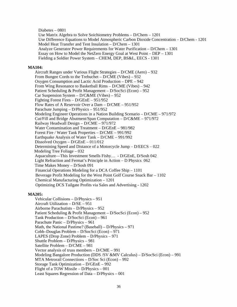
36

Diabetes – 0801 Use Matrix Algebra to Solve Soichiometry Problems – D/Chem – 1201 Use Difference Equations to Model Atmospheric Carbon Dioxide Concentration – D/Chem - 1201 Model Heat Transfer and Tent Insulation – D/Chem – 1301 Analyze Generator Power Requirements for Water Purification – D/Chem – 1301 Essay on How to Model the NetZero Energy Goal at West Point – DEP – 1301 Fielding a Soldier Power System – CHEM, DEP, BS&L, EECS - 1301

MA104: Aircraft Ranges under Various Flight Strategies – D/CME (Aero) – 932 From Bungee Cords to the Trebuchet – D/CME (Vibes) – 932 Oxygen Consumption and Lactic Acid Production – DPE – 942 From Wing Resonance to Basketball Rims – D/CME (Vibes) – 942 Patient Scheduling & Profit Management – D/SocSci (Econ) – 952 Car Suspension System – D/C&ME (Vibes) – 952 Fighting Forest Fires – D/GEnE – 951/952 Flow Rates of A Reservoir Over a Dam – D/CME – 951/952 Parachute Jumping – D/Physics – 951/952 Modeling Engineer Operations in a Nation Building Scenario – D/CME – 971/972 Cut/Fill and Bridge Abutment/Span Computation – D/C&ME – 971/972 Railway Headwall Design – D/CME – 971/972 Water Contamination and Treatment – D/GEnE – 981/982 Forest Fire / Water Tank Properties – D/CME – 991/992 Earthquake Analysis of Water Tank – D/CME – 991/992 Dissolved Oxygen – D/GEnE – 011/012 Determining Speed and Distance of a Motorcycle Jump – D/EECS – 022 Modeling Tree Foliage – 032 Aquaculture—This Investment Smells Fishy… - D/GEnE, D/Sosh 042 Light Refraction and Fermat’s Principle in Action – D Physics 062 Time Makes Money – D/Sosh 091 Financial Operations Modeling for a DCA Coffee Ship – 1101 Beverage Profit Modeling for the West Point Golf Course Snack Bar – 1102 Chemical Manufacturing Optimization – 1201 Optimizing DCS Tailgate Profits via Sales and Advertising - 1202 MA205: Vehicular Collisions – D/Physics – 951 Aircraft Utilization – D/SE – 951 Airborne Parachutists – D/Physics – 952 Patient Scheduling & Profit Management – D/SocSci (Econ) – 952 Tank Production – D/SocSci (Econ) – 961 Parachute Panic – D/Physics – 961 Math, the National Pastime? (Baseball) – D/Physics – 971 Cobb–Douglas Problem – D/SocSci (Econ) – 971 LAPES (Drop Zone) Problem – D/Physics – 971 Shuttle Problem – D/Physics – 981 Satellite Problem – D/CME – 981 Vector analysis of truss members – D/CME – 991 Modeling Bangalore Production (DDS /SV &MV Calculus) – D/SocSci (Econ) – 991 MTA Metrorail Connections – D/Soc Sci (Econ) – 992 Storage Tank Optimization – D/GEnE – 992 Flight of a TOW Missile – D/Physics – 001 Least Squares Regression of Data – D/Physics – 001

37

Counterbattery Target Acquisition – D/Physics – 011 Modernizing Camera Product Lines – D/SocSci (Econ) – 011 Incoming Interception in BMD – D/Physics – 021 Treating Motor Pool Runoff – D/GEnE – 021 Modeling the Spread of Information and Influence – 1001 Modeling the Growth of an Insurgency – 1101 Analyzing Opium Trade in Afghanistan – 1201 Tidal Power – 1301 Wind Turbine Analysis – 1301 Modeling Drug Assimilation in the Bloodstream – 1302 Modeling the Spread of Disease – 1302 Modeling Rocket/Projectile Flight – D/Physics - 1401 MA206: Pollution Levels in the Great Lakes – D/GEnE – 951/952 Statistical Analysis of Hudson River Pollution Data – D/GEnE – 981 Markov Chain Model of Dow Jones Industrial Average – D/SocSci– 982 Statistical Analysis of Elementary Circuits – D/Physics – 982 Call for Artillery – D/EECS – 981 The Dam Problem – D/CME – 992 Capacitors in Circuits – D/Physics – 082 Price Controls and Gasoline in Iraq – D/SocSci - 091 The interdisciplinary goal embodies the belief that early mastery of mathematics skills produces in cadets the realization that they can indeed formulate and analyze interesting problems arising in engineering, science, business, and many other fields. Our experience is that this realization increases cadet motivation. We and the application departments have seen benefits of this increased motivation as cadets move from core mathematics into their disciplines. Our interdisciplinary material is public domain – any reader interested in these materials can find many of the ILAPs at the Department of Mathematical Science’s web page (www.dean.usma.edu/math/), or can contact the core program director for more information. Beginning in AY 12-13, the focus of our interdisciplinary work has been built around the theme of operational energy. The math department has been part of the leadership team in an Academy initiative involving interdisciplinary collaboration. This effort began with participation as one of 25 institutions in a Project Kaleidoscope (PKAL) initiative to enhance interdisciplinarity within core programs. The West Point team chose the topic of energy for preliminary efforts as it is both a timely real world issue and ties into the designation of West Point as a “Net Zero” installation. The department is participating as part of the Academy Core Interdisciplinary Team (CIT) with 8 departments to include energy themed work within the core courses so that students explore the topic from multiple perspectives and see ties between those disciplines in the context of one important issue.

38

LIAISON PROFESSORS “Servicing What We Sell”

Most departments at USMA rely on at least some portion of the core mathematics program to prepare cadets for studies in their Department. Additionally, the Department of Mathematical Sciences has found that the study of mathematical principles and methods is almost always made easier by considering problems in applied settings with realistic scenarios. In order to facilitate success in both of these areas, the Department of Mathematical Sciences has instituted a liaison program in which a tenured faculty member is designated as the Liaison Professor primarily responsible for coordination with a particular client Department. The designations for this academic year are as follows: DEPARTMENT LIAISON PROFESSOR PHONE OFFICE BS&L (Human Factors) LTC Krista Watts x7685 TH226C Chemistry & Life Science COL Jerry Kobylski x5608 TH251 C&ME LTC Tony Johnson x7217 TH235B EE&CS LTC Doug McInvale x4544 TH255A GEnE COL Tina Hartley x2276 TH239A Physics Fr. Gabe Costa x5625 TH235A COL Tina Hartley x2276 TH239A Soc Sci (Econ) LTC Mike Yankovich x2807 TH225 Systems Eng LTC Doug McInvale x4544 TH255A COL Tina Hartley has primary responsibility for oversight of the Liaison Professor program. The major focus of this program is to achieve a more integrated student MSE experience by promoting coordination and collaboration between the Department of Mathematical Sciences and the other MSE Departments. The role of the Liaison Professor is to serve as the principal point of contact for members of the client department. The Liaison Professor fields questions, accepts suggestions, and works issues from the client department with respect to course material, ILAPs, procedures, timing, and any other matters of mutual interest. Additionally, the Liaison Professor is a first point of contact for course directors in the Department of Mathematical Sciences who are looking for examples and applications appropriate to their course and need referrals. This program is not intended to preclude closer coordination (for instance, at the course director or instructor level), but rather is intended to provide a continuing source of information and input at the senior faculty level who can ensure that inter-departmental cooperation is accomplished across several courses in a consistent fashion, as required.

39

UNITED STATES MILITARY ACADEMY MATHEMATICAL RECALL KNOWLEDGE

The following constitutes a basic mathematical vocabulary that will be built upon during each cadet’s four-semester core mathematics experience and in his or her future math/science/engineering courses. Once each of these basic ideas has been covered in class, each cadet can be required to reproduce, upon demand in any future lesson of any math/science/engineering course, that idea exactly as shown here. Annotated beside each heading or item is the course number in which the cadet is responsible for each item . These items are recall knowledge - cadets are also required to be proficient in the more conceptual, less-verbatim ideas and skills reflected in each core math course’s Course Objectives section of this document.

ALGEBRA (103/1)

1. ax2 + bx + c = 0 = = > x = −b +− b2 − 4ac

2a 2. ab . ac = a b +c

3. (ab )c = ab c 4. ab

ac = ab −c

5. y = logb x => x = by 6. logb bx = b logb x = x

7. logb xa = a logb x 8. logb ac = logb a + logb c

9. logb ac = logb a - logb c 10. logb a = log a

log bc

c

ANALYTIC GEOMETRY (103/1)

Rectangle: Area = lw Perimeter = 2l + 2w

Circle: Area = πr2 Circumference = 2πr

Rectangular Solid: Volume = lwh Surface Area = 2lw + 2lh + 2hw

Cylinder: Volume = πr2 l Surface Area = 2πr2 + 2πrl

Sphere: Volume = 43 π r3 Surface Area = 4 π r 2

Distance between (x1, y1) and (x2, y2) = 2)21(

2)21( yyxx −+−

TRIGONOMETRY (103/1)

With reference to the right triangle:

2π radians = 360 degrees sin θ =

yr cos θ =

xr tan θ =

yx

tan θ = sin θcos θ x2 + y2 = r2 sin2θ + cos2θ = 1

cot θ = 1

tan θ sec θ = 1

cos θ csc θ = 1

sin θ

40

RELATIONSHIPS (MA103/1)

Corresponding sides of similar triangles are proportional Distance = average rate × time

DIFFERENTIATION (MA 104)

1. ddx (a) = 0 (104) 2.

ddx (x) = 1 (104)

3. ddx (au ) = a

dudx (104) 4

ddx (u + v) =

dudx +

dvdx (104)

5. ddx (uv) = u

dvdx + v

dudx Product Rule (104) 6. v =

v dudx − u

dvdx

v2ddx

u

Quotient Rule (104)

7. ddx (un) = nun−1

dudx Power Rule (104) 8.

ddx [f(u)] =

ddu [f(u)]

dudx Chain Rule (104)

9. ddx (sin u) = cos u

dudx (104) 10.

ddx (cos u) = −sin u

dudx (104)

11. ddx(eu) = eu

dudx (104) 12.

ddx (ln u) = dx

1u

du (104)

INTEGRATION (MA 205)

13. ∫ a dx = ax + C (205) 14. ∫ (u + v) dx = ∫ u dx + ∫ v dx (205)

15. ∫ xn dx = xn+1

n+1 + C (n ≠ −1) (205) 16. ∫ eax dx = Ceax

a + (205)

17. Understand and be able to apply the 18. ∫ duu = ln |u| + C (205)

Substitution Rule (205)

19. ∫ sin (ax) dx = − 1a cos (ax) + C (205) 20. ∫ cos (ax) dx = C

1a sin (ax) + (205)

21. If f is integrable on [a, b], then ∫ −=b

a

aFbFdxxf )()()( where )(xfdxdF

=

(Fundamental Theorem of Calculus) (205)

VECTOR CALCULUS (MA104)

22. |A− >

| = j + a2ka

2i + a

2 (104)

24. =× BA

|A− >

| |B− >

| |sin θ| (104)

23. θcosBAkbkajbjaibiaBA

=++=• (104)

25.∇f = k zf

+ j yf

+ i xf

∂

∂

∂

∂

∂

∂ (104)

41

PROBABILITY & STATISTICS (MA 206) 26. PDFs and CDFs: (206) Discrete: PDF: )()( xpxXP == . CDF: ∑

≤

=≤xy

ypxXP )()( .

Continuous: PDF: )(xf is used to find probabilities - ∫=≤≤b

a

dxxfbXaP )()( .

CDF: ∫∞−

=≤=x

dyyfxXPxF )()()( .

27. The total accumulation of a probability distribution function is 1. (206)

Discrete: 1)( =∑∀x

xp Continuous: 1)( =∫∞

∞−

dxxf

28. Calculate and interpret the expected value (mean) of a random variable. (206)

Discrete: ∑∀

⋅=x

xpxXE )()( Continuous: ∫∞

∞−

⋅= dxxfxXE )()(

29. Calculate and interpret the variance of a random variable. (206) The variance is an expected value: 222 )(])[()( µµ −=−= XEXEXV . 30. Percentiles of random variables including the median (50th percentile). (206) 31. Central Limit Theorem: Let X X X n1 2, ,... , be a random sample from any population with a finite mean

and variance. Then, if n is sufficiently large, nXX i∑= and ∑= iXT0 are approximately normally distributed. (206)

42

PROPERTIES OF FUNCTIONS (103/1)

x

f(x)f x( ) .8 x. 2

f x( )

x

f(x) = mx + b

f x( ) sin x( )

f x( )

x2

1

1

2

π π20

f(x) = sin (x)

x

f(x)

f x( ) cos x( )

f x( )

x2

1

1

2

π x

f(x) f(x) = cos (x)

0 π2

g x( ) tan x( )

g x( )

x

πx

f(x)

π−

f(x) = tan (x)

0

asymptote

f x( ) ex

f x( )

x

f(x)f(x) = e x

asymptotex

(0,1)

x

f(x)f x( ) e x

f x( )

x

asymptote

(0,1)

f(x) = e -x

x

f(x)f x( ) ln x( )

f x( )

x

f(x) = ln (x)

(1,0)

asymptote

43

UNITED STATES MILITARY ACADEMY REQUIRED SKILLS IN SCIENTIFIC COMPUTING

The following list constitutes the basic, required scientific computing skills that you will learn and use during your four-semester core mathematics experience and in your future math/science/engineering courses. Once each of the listed topics is covered in class, you must be able to execute this skill upon demand in any future lesson or course. Reference books, for the respective computing system, are the chief source of information for learning these skills. Annotated beside each item is the course, which denotes the exact point in time you are responsible for that particular item (e.g. 103 indicates responsibility for that skill following MA103).

LAPTOP SKILLS (MATHEMATICA and MS EXCEL) The following are all laptop (or desktop) computer skills. Most can be accomplished in either Mathematica or Excel, but some are easier in one package. As you become proficient in each skill, it is your job to decide which tool is the right one for the task at hand. 1. Enter a recursive relationship and evaluate analytically, numerically and graphically:

E.g. Given the difference equation 21 3 naa nn +=+ (103)

a. Find 100a .

b. Display a table of “n” and “ na ” values.

c. Graph the time-series plot of na . 2. Perform basic matrix and vector operations a. Given 2 matrices, compute (if defined) their sum and product. (103) b. Find the inverse of a given square matrix (if it exists). (103) c. Find the eigenvalues and eigenvectors of a given matrix. (103) d. Find the magnitude of a given vector. (104) e. Given 2 vectors, compute their dot product and cross product. (103/104) 3. Perform matrix operations on linear systems of equations in two and three variables:

E.g. Given the linear system of equations,

=

474

523487652

zyx

a. Solve the system of equations. (103) b. Perform row reduction operations on the augmented matrix. (103) 4. Use the Solve or FindRoot commands in Mathematica to find the roots of a polynomial or transcendental function (both real and complex) or to solve simultaneous equations. E.g. a. Find the roots of the functions 08147 23 =+−− rrr (103) b. Find the roots of the functions ex – 2 = 0 c. Solve to find the point of intersection between 732 =+ yx and 4=+− yx 5. Define and evaluate a function at a specific point in Mathematica and Excel. (103) f(x) = 2x2 + 3x – 24 e2x g(x) = sin (3x) + ex – 2 ln(x) 6. Plot a function or several functions over a specified domain. (103)

44

7. Use the Excel Solver to minimize the squared error when fitting models to data. (103) Minimize the SSE between known distributions and the EDF. (206) 8. Plot 3-dimensional objects (surfaces, space curves, and level curves): E.g. Plot the space curve (104) [ ]π,0 , )sin( 2 )( 2 ∈++= tktjtittr

E.g. Plot the surface 164

22 yxz += . (104)

E.g. Plot the level curves for x2 + y2 = k (104) 9. Evaluate limits: (103/104)

E.g. Evaluate 255

lim 25 −

−→ x

xx

.

E.g. Evaluate 73

2lim

1

−

+ −

∞→ xxx

x .

10 Evaluate derivatives:

E.g. Given the function )2(sin1 3 -xx+x

y = ,

a. Find the derivative. (104) b. Plot the derivative. (104)

E.g. Given the function )-sin(2+1

),( 3 yxy

yxf = , find xf

∂∂

and yf

∂∂

. (104)

E.g. Given the function 22),( xyyxyxf += ,

a. Find the partial derivatives .2

22

,

,

xf

yxf

xf

∂

∂∂∂

∂∂∂

(104)

b. Find the gradient of f(x,y) at the point (2,3). (104) c. Find the directional derivative of f(x,y) at the point (2,3) in the (104) direction of ji

4 2 − .

11. Solve nonlinear systems of equations: a. Solving for relative extrema (104) b. Constrained optimization (Lagrange) (104) 12. Calculate Riemann sums to approximate net change. (205) 13. Evaluate definite and indefinite integrals:

E.g. Evaluate ∫x

adyyf )( . (205)

45

E.g. Evaluate ∫ − dxexx x ))ln(( (205)

E.g. Evaluate ( )∫ +π

0

2 )2cos( dxxx . (205)

E.g. Evaluate ( )∫ ∫3

0

2

0

2 dxdyyx (205)

E.g. Evaluate ( )∫ ∫1

0

2

0

3 3y

xy dydxey . (205)

E.g. Evaluate ( ) ( )

, 6

12sin

6 12

sin3

0dx

xmxn

−

∫− ππ

(364)

for m = n and m ≠ n . 14. Calculate distance traveled along a curve using the concept of arc length. (205) 15. Differential Equations (DE):

E.g. Given the DE , 2)cos( −+= −xexdxdy

π

a. Plot the direction (slope) field of the DE. (205) b. Graphically approximate a solution curve to the DE for y(0) = 2. (205) c. Use Euler’s Method to find a numerical approximation for y(3) given y(0) = 2. (205) d. Verify a given solution to the DE (205) 16. Probability and Statistics: a. Fit a regression line to given data by minimizing the SSE. (206) b. Compute sample statistics from a data set. (206)

c. Plot a histogram. (206) c. Create an empirical CDF from a given matrix of data. (206)

d. Analyze data with descriptive statistics and descriptive plots. (206) e. Integrate known distributions to determine probabilities. (206) f. Calculate expected value and population variance using integration. (206) g. Calculate the inverse CDF using FindRoot or Solve commands. (206) . h. Simulate data (generate pseudo-random data) (206)

i. Perform linear regression and interpret the output (206)

17. Seek on-line HELP to learn new commands, uses, and methods, as well as to troubleshoot one’s own efforts.

MS-WORD, with Graphics Objects from other Packages

18. Create a formal document in electronic form that includes textual, graphical, numerical, and analytical modeling and analysis. (103)

46

REQUIRED MATHEMATICAL SKILLS FOR ENTERING CADETS

Cadets enter the United States Military Academy (USMA) with different backgrounds in mathematics. To successfully begin work in math, science, and engineering (MSE) courses at USMA, cadets must arrive with knowledge of certain mathematical skills and concepts. The MSE Committee deems the items below to be fundamental skills and concepts that all entering cadets must possess. Early in Cadet Basic Training, the Department of Mathematical Sciences administers a “Gateway” exam to assess fundamental skills. Therefore, we encourage incoming cadets to evaluate their mathematics skills and work at remediation of any deficiencies prior to arriving at USMA. The Department of Mathematical Sciences administers two additional “Gateway” exams during the first semester in MA103 (Discrete Dynamical Systems and Introduction to Calculus). Self-paced texts and software files offer opportunities for self-remediation. Failure to pass at least one “Gateway” exam at mastery level (≥ 80%) may result in having to retake MA103 during the second semester instead of continuing into MA104 (Calculus and Differential Equations), or other scheduled remediation. Cadets enrolled in MA100 who do not demonstrate proficiency in these fundamental mathematics skills by the end of their first year may be separated from USMA.

Almost any high school algebra book is a suitable reference for these fundamental skills. An incoming cadet can obtain additional exam resources by going to the following link: http://www.dean.usma.edu/math/courses/MA103/ProspectiveStudents/CandidateWeb.htm

Note: All calculations must be done without the use of technology (i.e., calculator). Some examples of skills are provided in parentheses. 1. Algebra and Real Numbers. a. Use symbols and operators to represent ideas and objects and the relationships existing between them. b. Understand the relationship between measures of the physical world. (Velocity, distance and time: On a 40-mile car trip to Middletown, NY, you drive the first twenty miles at 40 mph and the last twenty miles at 60 mph. What is your average speed during the trip?) c. Know and apply the following algebraic properties of the real number system: identity, associative, commutative, inverse, and distributive. d. Express numbers using scientific notation. (Express 0.004312 in scientific notation.) 2. Radicals and Exponents. a. Convert between radical and rational exponent

form. (Transform 21+x to the rational exponent

form 21

)2(−

+x .)

b. Manipulate algebraic expressions that contain

integer and rational exponents. (Simplify 32

23

274−−

⋅ .)

3. Algebraic Expressions. a. Add, subtract, multiply, and divide algebraic expressions. (Find the remainder when x3 – 7x2 + 9x is divided by x – 2.) b. Simplify algebraic expressions. (Expand and simplify (x-3) (x-2) (x-1).) 4. Factoring / Prime Numbers a. Write a number as the product of factors. (Write 42 as the product of prime factors.) b. Solve for the roots of a polynomial by factoring. (Find the roots of x2 – 5x + 6 = 0.) 5. Linear Equations, Inequalities and Absolute Values. a. Solve two simultaneous linear equations by graphing and by substitution. (Use a graph to estimate the point of intersection of the lines 2x + 3y = 7 and –x + y = 4. Verify your result using back substitution.) b. Solve linear equations and inequalities [graphically and algebraically]. (Solve 5(3-x) > 2(3-2x) for x.) c. Solve linear equations and inequalities with absolute values. (Solve | x - 4 | ≥ 3 for x.)

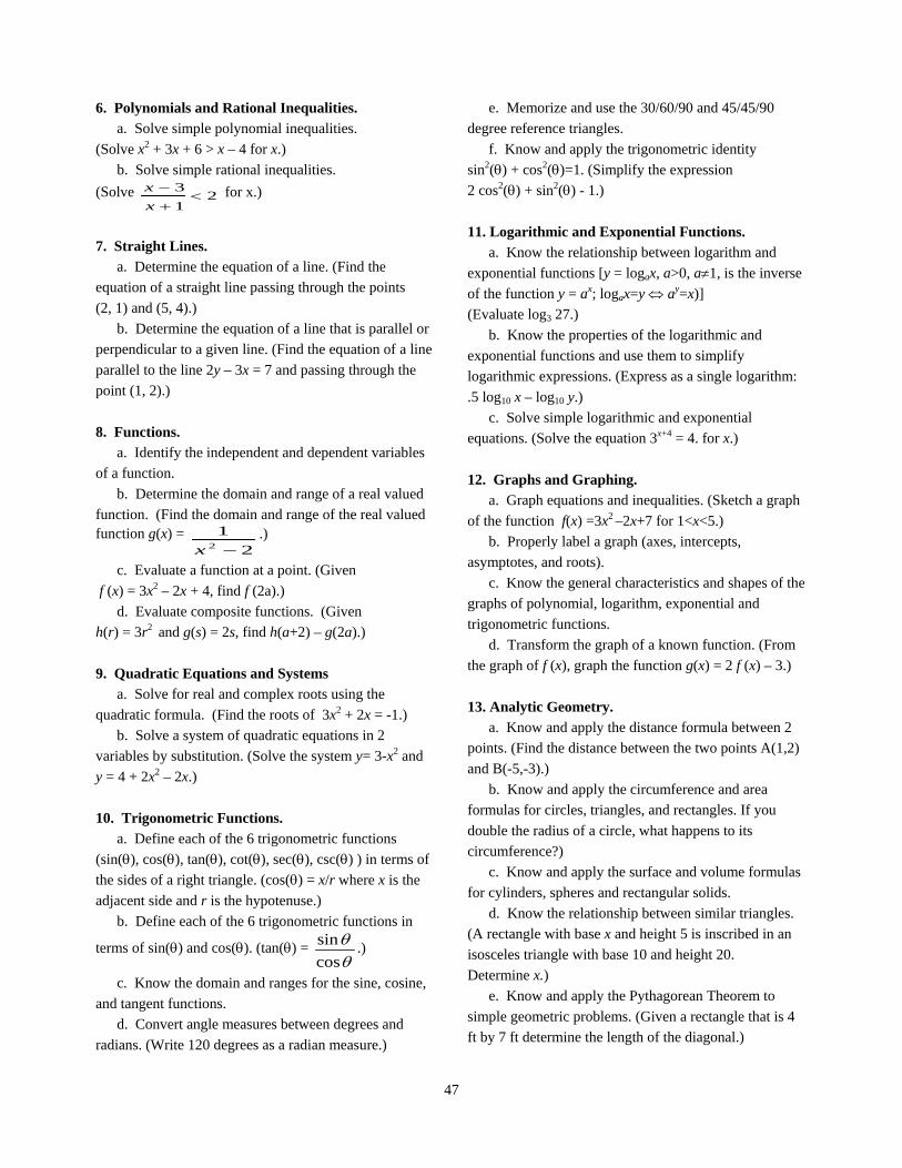
http://www.dean.usma.edu/math/courses/MA103/ProspectiveStudents/CandidateWeb.htm

47

6. Polynomials and Rational Inequalities. a. Solve simple polynomial inequalities. (Solve x2 + 3x + 6 > x – 4 for x.) b. Solve simple rational inequalities. (Solve 2

13

<+

−

xx for x.)

7. Straight Lines. a. Determine the equation of a line. (Find the equation of a straight line passing through the points (2, 1) and (5, 4).) b. Determine the equation of a line that is parallel or perpendicular to a given line. (Find the equation of a line parallel to the line 2y – 3x = 7 and passing through the point (1, 2).) 8. Functions. a. Identify the independent and dependent variables of a function. b. Determine the domain and range of a real valued function. (Find the domain and range of the real valued function g(x) =

21

2 −x.)

c. Evaluate a function at a point. (Given f (x) = 3x2 – 2x + 4, find f (2a).) d. Evaluate composite functions. (Given h(r) = 3r2 and g(s) = 2s, find h(a+2) – g(2a).) 9. Quadratic Equations and Systems a. Solve for real and complex roots using the quadratic formula. (Find the roots of 3x2 + 2x = -1.) b. Solve a system of quadratic equations in 2 variables by substitution. (Solve the system y= 3-x2 and y = 4 + 2x2 – 2x.) 10. Trigonometric Functions. a. Define each of the 6 trigonometric functions (sin(θ), cos(θ), tan(θ), cot(θ), sec(θ), csc(θ) ) in terms of the sides of a right triangle. (cos(θ) = x/r where x is the adjacent side and r is the hypotenuse.) b. Define each of the 6 trigonometric functions in

terms of sin(θ) and cos(θ). (tan(θ) = θθ

cossin .)

c. Know the domain and ranges for the sine, cosine, and tangent functions. d. Convert angle measures between degrees and radians. (Write 120 degrees as a radian measure.)

e. Memorize and use the 30/60/90 and 45/45/90 degree reference triangles. f. Know and apply the trigonometric identity sin2(θ) + cos2(θ)=1. (Simplify the expression 2 cos2(θ) + sin2(θ) - 1.) 11. Logarithmic and Exponential Functions. a. Know the relationship between logarithm and exponential functions [y = logax, a>0, a≠1, is the inverse of the function y = ax; logax=y ⇔ ay=x)] (Evaluate log3 27.) b. Know the properties of the logarithmic and exponential functions and use them to simplify logarithmic expressions. (Express as a single logarithm: .5 log10 x – log10 y.) c. Solve simple logarithmic and exponential equations. (Solve the equation 3x+4 = 4. for x.) 12. Graphs and Graphing. a. Graph equations and inequalities. (Sketch a graph of the function f(x) =3x2 –2x+7 for 1<x<5.) b. Properly label a graph (axes, intercepts, asymptotes, and roots). c. Know the general characteristics and shapes of the graphs of polynomial, logarithm, exponential and trigonometric functions. d. Transform the graph of a known function. (From the graph of f (x), graph the function g(x) = 2 f (x) – 3.) 13. Analytic Geometry. a. Know and apply the distance formula between 2 points. (Find the distance between the two points A(1,2) and B(-5,-3).) b. Know and apply the circumference and area formulas for circles, triangles, and rectangles. If you double the radius of a circle, what happens to its circumference?) c. Know and apply the surface and volume formulas for cylinders, spheres and rectangular solids. d. Know the relationship between similar triangles. (A rectangle with base x and height 5 is inscribed in an isosceles triangle with base 10 and height 20. Determine x.) e. Know and apply the Pythagorean Theorem to simple geometric problems. (Given a rectangle that is 4 ft by 7 ft determine the length of the diagonal.)

48

SAMPLE FUNDAMENTAL CONCEPT EXAM I

1. Completely simplify 113�1−

23�

2. Solve 7𝑥 = 149

for 𝑥 3. Expand the product (3𝑥 − 4)(5 − 2𝑥) and combine like terms.

4. Find all roots of 𝑥2 − 10𝑥 + 23 = 0. 5. Find the distance between the points (1,6) and (6,18). 6. Solve 𝑥2 + 3𝑥 ≤ 4 for 𝑥. 7. Find an equation of the line that passes through the points (−1,0) and (2,6). 8. If the independent variable of 𝑤(𝜃) = 2𝜃2 is restricted to values in the interval [2,5], what is the

interval of all possible values of the dependent variable? 9. Completely simplify 2 cot 𝑥 sec 𝑥 sin 𝑥.

10. Completely simplify �3𝑎−2

𝑏�−2

.

11. Solve �3𝑥 = 2 − 7𝑦𝑦 = 𝑥 − 5

� for 𝑥 and 𝑦.

12. Given 𝑔(𝑡) = 2 + 3𝑡 and ℎ(𝑠) = 4𝑠2, evaluate 𝑔(3) − ℎ(2). 13. Graph 𝑦 = sin 𝑥 − 2 on the domain [0,2𝜋]. Label the axes. 14. If you double the length of the sides of a cube, by how much is the volume affected? 15. Completely simplify 3

(log4 8 + log4 2) .

16. Find an equation of the line that is parallel to the line −4𝑥 + 8𝑦 = 12 and passes through the point

(1,1). 17. Solve 𝑥2 + 7𝑥 − 8 = 0 for 𝑥.

18. Completely simplify � �𝑥𝑦63 �6

.

49

19. Given the right triangle below, what is tan𝜃?

20. Solve 3 + 𝑥 > −(𝑥 − 2) for 𝑥.

10

B

A C θ

6

50

SAMPLE FUNDAMENTAL CONCEPT EXAM II

1. Write 42 as a 𝑝𝑟𝑜𝑑𝑢𝑐𝑡 of its prime factors.

2. Write √𝑥23 without using radical notation.

3. If Joe runs the first mile of the APFT in 5 minutes 40 seconds, and he wants to finish the 2-mile course in less than 12 minutes 40 seconds, at what speed must he run the remaining mile?

4. Solve |𝑥 − 5| = 7 for 𝑥.

5. Find the equation of the line that passes through the points (−2,1) and (−3,1).

6. What is the range of the function ℎ(𝑥) = −𝑥2?

7. Solve 𝑦 = 2𝑥 − 5𝑦2 = 4𝑥2 + 5 for 𝑥 and 𝑦.

8. If the hypotenuse of a 30-60-90 right triangle measures 6 inches, how long is the side of the triangle that

is opposite from the 30° angle?

9. Solve 4 = log3 𝑥 for 𝑥.

10. Given that 𝑓(𝑥) = sin 𝑥, write the function that shifts 𝑓(𝑥) to the right by 3 units.

11. Write 6.371 𝑥 10−5 in decimal notation.

12. Expand the product (𝑥 − 5)(5 − 𝑥).

13. Solve for the roots of 𝑔(𝑥) = 𝑥2 − 3𝑥 − 10.

14. Solve 𝑥2 − 5𝑥 + 3 > 5 − 4𝑥 for 𝑥.

15. Find the equation of the line that pass through the point (1,2) and that is parallel to the line 𝑦 = −3𝑥 + 4.

16. Evaluate 𝑗(𝑥) = √𝑥2 + 5 at 𝑥 = 𝑎.

17. What is the domain of the function 𝑚(𝜃) = sin(3𝜃)?

18. Completely simplify log3 𝑎 + log3 𝑏.

19. Sketch a graph of 𝑦 = 𝑥3 + 3. Label 3 points on your sketch.

20. How long is the diagonal of a 3" x 5" rectangle?

51

SAMPLE FUNDAMENTAL CONCEPT EXAM III

1. Write 5,226,000 in scientific notation.

2. Completely simplify √16𝑢124 . Assume all variables represent positive numbers.

3. Expand the product (3𝑥 + 7)(3𝑥 − 7) and combine like terms.

4. Find all roots of 𝑥2 + 8𝑥 = 1.

5. Find the distance between the points (−2,−1) and (−6,−9).

6. Solve 𝑥2 − 5𝑥 ≤ −4 for 𝑥.

7. What is the range of the function ℎ(𝑥) = −𝑥2?

8. Solve 𝑦 = 2𝑥 − 5𝑦2 = 4𝑥2 + 5 for 𝑥 and 𝑦.

9. If the hypotenuse of a 30-60-90 right triangle measures 6 inches, how long is the side of the

triangle that is opposite from the 30° angle?

10. Solve 4 = log3 𝑥 for 𝑥.

11. Given the triangle below with side 𝐷𝐸 parallel to side 𝐵𝐶 and lengths in 𝑓𝑒𝑒𝑡, what is the length of side 𝐵𝐷?

12. If the diagonal of a rectangle measures 6 𝑖𝑛𝑐ℎ𝑒𝑠, and its short side measures 2 𝑖𝑛𝑐ℎ𝑒𝑠, what is the area of the rectangle?

13. Sketch the graph of 𝑦 = 𝑥2 − 4. Label three points on the graph.

14. Find the equation of the line that passes through the points (3,4) and (5,4).

15. What is the domain of the function ℎ(𝑥) = sin 𝑥?

16. Given 𝑔(𝑡) = 6𝑡 − 2 and ℎ(𝑠) = 5𝑠3, find 𝑔(ℎ(−1)).

17. Completely simplify 2 cot 𝑥 sec 𝑥 sin 𝑥.

10

4 6

E C

B A D

52

18. Write 42 as a product of its prime factors.

19. Solve |𝑥 − 5| = 7 for 𝑥.

20. Completely simplify log4 36 − log4 9.

53

HISTORY OF THE DEPT OF MATHEMATICAL SCIENCES AT USMA A teacher affects eternity; he can never tell where his influence stops. -- Henry Adams The Department of Mathematical Sciences, USMA, has a rich history of contributing to the education of cadets as confident problem solvers and of developing its faculty as effective teachers, leaders, and researchers. The story of mathematical education at West Point is full of interest: faculty curriculum developments, teaching methods and tools, and technological equipment. Many of the Department's advances have been exported outside the Academy to be employed by other civilian and military educational institutions. EARLY BEGINNINGS: The actual teaching of mathematics at West Point dates from even before the Academy was established. In 1801, George Baron taught a few Cadets of Artillery and Engineers some of the fundamentals and applications of algebra. The Academy at West Point was instituted by act of Congress and signed into law by President Thomas Jefferson on 16 March 1802. The first acting Professors of Mathematics were Captains Jared Mansfield and William Barron. They taught the first few cadets topics in algebra, geometry, and surveying. CONTRIBUTIONS TO THE NATION: Since the Academy was the first scientific and technical school in America, the early mathematics professors at USMA had the opportunity to make significant contributions not only to the Academy, but also to other American colleges. Perhaps the most prominent contributors were the early 19th century department heads Charles Davies and Albert E. Church. The work of these two professors had a significant impact on elementary schools, high schools, and colleges across the country. Davies became the Professor of Mathematics in 1823. He was one of the most prolific textbook authors of his day, writing over 30 books from elementary arithmetic to advanced college mathematics. His books were used in schools throughout the country from grade school to college. He had tremendous influence on the educational system of America throughout the 19th century. Albert Church succeeded Davies in 1837, and served as Department Head for the next 41 years. Another influential author, he published seven college mathematics textbooks. PRODUCING LEADERS FOR THE NATION: Faculty from the Department have been notable military leaders for the country. Robert E. Lee was a standout cadet-instructor in the Department, Omar Bradley served as an Instructor for four years, Harris Jones and William Bessell were Deans of the Academic Board at USMA for a total of 15 years, and Department Heads Harris Jones, William Bessell, Charles Nicholas, John Dick, and Jack Pollin served impressively during two world wars. The unique technical curriculum in place at the Academy during the middle of the 19th century produced many successful mathematicians and scientists for the country at large. West Point graduates Horace Webster, Edward Courtenay, Alexander Bache, James Clark, Francis Smith, Richard Smith, Henry Lockwood, Henry Eustis, Alexander Stewart, and William Peck filled positions as professors of mathematics or college presidents at other schools such as the U. S. Naval Academy, Geneva College, University of Virginia, University of Pennsylvania, University of Mississippi, Yale, Brown, Harvard, Columbia, Virginia Military Institute, Cooper Institute, and Brooklyn Polytechnic Institute. Two mathematics department heads became college presidents after leaving USMA; Alden Partridge founded and became the first president of Norwich University, and David Douglass served as president of Kenyon College in Ohio for four years. Jared Mansfield was appointed surveyor-general of the Northwest Territory, and Ferdinand Hassler became superintendent of the United States Coastal Survey. Capable individuals such as these exported the West Point model of undergraduate mathematics education throughout the nation. While the faculty at USMA has been primarily military, the Department has benefited from civilian visiting professors since 1976. As part of the goal for civilianization of 25% of the faculty by 2002, begun in 1992, the Department established in 1994 a Center for Faculty Development in Mathematics. This Center establishes faculty development models and curricula and provides for the development of the "Davies Fellows", who serve as rotating civilian faculty members. HISTORICAL AND LIBRARY HOLDINGS: Sylvanus Thayer's first task before assuming the Superintendancy in 1817 was to tour the technical institutions of Europe and assess what features USMA could use to advantage. One of Thayer's many accomplishments was to obtain numerous mathematics and science

54

books from Europe. Thayer's book collection included many of the finest books available at that time. His books provided a solid foundation for the USMA library to build upon. Today, the West Point Library has one of the finest collections of pre-20th century mathematics books in the world. Also during the middle of the 19th century, the Academy instructors used elaborate physical models made by Theodore Oliver to explain the structures and concepts of geometry. This magnificent collection of string models is still in the Department today. CURRICULAR DEVELOPMENT: After Thayer studied the military and educational systems of Europe, he reorganized the Academy according to the French system of the Ecole Polytechnic. The Department of Mathematics faculty (which included as Professor the distinguished scientist and surveyor Andrew Ellicott, and the famous French mathematician Claude Crozet whom Thayer recruited during his European trip to bring to USMA and America his expertise in Descriptive Geometry, advanced mathematics, and fortifications engineering) combined the French theoretical mathematics program with the practical methods of the English to establish a new model for America's program of undergraduate mathematics. This program of instruction in Mathematics grew over several decades and was emulated by many other schools in the country. The initial purpose of the Military Academy was to educate and train military engineers. Sylvanus Thayer, the "Father of the Military Academy" and Superintendent from 1817-1833, instituted a four-year curriculum with supporting pedagogy to fulfill this purpose. Thayer's curriculum was very heavy in mathematics; from Thayer's time to the late 1800's, cadets took the equivalent of 54 credit hours of mathematics courses. The topics covered in these courses were algebra, trigonometry, geometry, descriptive geometry (engineering drawing), analytic geometry, and calculus. Over the years, the entering cadets became better prepared and fewer of the elementary subjects were needed. During Davies' tenure (1823-37), calculus was introduced as a requirement for all cadets, and was used in the development of science and engineering courses. The time allotted for the mathematics curriculum decreased to 48 credit hours by 1940, and to 30 credit hours by 1950. During the 1940's, courses in probability & statistics and in differential equations were introduced into the core curriculum and a limited electives program was started for advanced students. In the 1960's, department head Charles Nicholas (previously one of the organizers of the Central Intelligence Agency) wrote a rigorous and comprehensive mathematics textbook (the "Green Death") that cadets used during their entire core mathematics program. With this text, he was able to adapt the mathematics program to keep up with the increasing demands of modern science and engineering. In the 1970's, Academy-wide curricular changes provided opportunities for cadets to major in mathematics. During the 1980's, a mathematical sciences consulting element was established that allowed faculty members and cadets to support the research needs of the Army. This type of research activity continues today in the Army Research Laboratory (ARL) Mathematical Sciences Center of Excellence and in the Operations Research Center (ORCEN). In 1990 the Department introduced a new core mathematics curriculum that included a course in discrete dynamical systems, with embedded linear algebra. In that same year, the department changed its name to the Department of Mathematical Sciences to reflect broader interests in applied mathematics, operations research, and computation. TECHNOLOGICAL DEVELOPMENT: USMA has a long history of technological innovation in the classroom. It was Crozet and other professors at USMA in the 1820's who were the first professors in the nation to use the blackboard as the primary tool of instruction. In 1944, the slide rule was issued to all cadets and was used in all plebe mathematics classes. During William Bessell’s tenure (1947-1959), the mathematics classrooms in Thayer Hall (a converted riding stable) were modernized with overhead projectors and mechanical computers. Bessell was also instrumental in establishing a computer center at West Point. The hand held calculator was issued to all cadets beginning in 1975, and pre-configured computers were issued to all cadets beginning in 1986. In recent years, the department has established a UNIX workstation lab, an NSF-funded PC lab, and has run experimental sections with notebook computers and with multimedia. NATIONAL COMPETITION: In the spring of 1933 West Point entered an interesting competition in mathematics. After USMA defeated Harvard at a football game the previous fall, a chance remark from President Lowell of Harvard to Superintendent Jones of USMA led the two schools to arrange a mathematics challenge match between the two schools with the two competing teams each composed of 12 second-year cadets. Army was the home team, so the Harvard competitors traveled by train to West Point. All the competitors took a test written by the president of the Mathematics Association of America. The New York Times, which had promoted the event with a series of articles in its sports section, reported the results. The West Point "mathletes" defeated Harvard in the competition that was the precursor to the national Putnam

55

Competition. Since its inception in 1984, the Academy has entered two three-person teams in the International Mathematics Competition in Modeling. USMA won the top prize in 1988, 1993, 2000, 2001, 2002, 2003, and 2004. During the first half of the 1990’s, the Department of Mathematical Sciences at USMA became recognized as one of the more progressive mathematics programs in the country. The Department developed a strong “7 into 4” program that is exciting as well as innovative. Throughout the 1990’s and into the 21st century, the Department of Mathematical Sciences has led the nation in curricular reform and in nurturing interdisciplinary cooperation and collaboration between and among partner disciplines. Project INTERMATH, a National Science Foundation grant to develop integrated curriculum and ILAPs, assisted in supporting these efforts. The USMA mathematics program has had great influence on mathematics education in America throughout its history, and strives to continue contributing to the improvement of mathematical education in America. For a more extensive exposition on the history of the Department, refer to http://www.dean.usma.edu/math/about/history/dept.htm.

http://www.dean.usma.edu/math/about/history/dept.htm

core mathematics at usma math/cmb-2014...... about the core mathematics ... mathematical skills and...

Documents