CORE PROFITABILITY OF COMMUNITY BANKS, 1985–2015

JARED FRONK Division of Insurance and Research

Federal Deposit Insurance Corporation 550 17th Street NW

Washington, DC 20429

19 SEPTEMBER 2017

ABSTRACT

The relatively low profitability reported by community banks since the 2008 financial crisis has sparked concerns about the core profitability of the community banking model. This paper constructs an econometric model using 31 years of data to estimate the impact of macroeconomic shocks on industry average pretax return on assets. After accounting for macroeconomic factors, the remaining unexplained variation is considered to be the core component of profitability. Core return on assets (ROA) is found to have been relatively stable between 1985 and 2015. It trended downward over the 1990s, but the effect of the financial crisis on industry composition has led to a reversal and a modest increase in core profitability. More than 80 percent of the post-crisis decline in profitability can be explained by negative macroeconomic shocks.

Keywords: community banking, bank profitability, business cycle JEL Codes: E32, G21, G28 The views here expressed are those of the author and no not necessarily reflect the official positions of the Federal Deposit Insurance Corporation.

1

Community Bank Profitability, 1985 to 2015

Profitability across FDIC-insured institutions fell to record lows during the financial crisis of 2008 and subsequent recession. In the years since, several measures of performance show the banking industry has rebounded. For example, by year-end 2015, noncurrent loans, loan-loss provisions, and net charge-offs had fallen to pre-crisis levels, and less than 5 percent of all institutions were unprofitable.

In contrast, profitability has remained well below pre-crisis levels, as measured by the average industry return on assets (ROA) of 1.03 percent at year-end 2015. Banks continue to feel the strain of an economy marked by slow growth and low interest rates. The industry’s net interest margin was just over 3 percent at year-end 2015, even as the share of longer-term assets with maturities over three years grew to just over one-third of total assets. It is reasonable to ask whether the weakness of the larger economic recovery has led to lackluster profitability growth in the banking industry.

Community banks—which accounted for 93 percent of all banks and 13 percent of total industry assets in 2015—have followed the same performance trends as the overall industry.1 Their noncurrent loans, loan-loss provisions, net charge-offs, and the percentage of unprofitable institutions have returned to pre-crisis levels, while profitability has remained stubbornly below pre-crisis levels. Pretax ROA for community banks was more than a full percentage point higher in 2015 than the lows seen during the crisis and stayed 20 to 30 basis points below the annual averages reported in the pre-crisis years.2

What accounts for the relatively low level of profitability among community banks in the post-crisis period? Have macroeconomic factors that are external to the banking industry placed downward pressure on profits, or have structural factors within the industry—such as business practices and the regulatory environment—changed the intrinsic profitability of the community banking model? I use an econometric model to separate pretax ROA, my chosen measure of bank profitability, into two parts: one part is attributable to cyclical variations in pretax ROA caused by macroeconomic factors, and the second part represents the core component of profitability and is attributable to structural factors that reflect the operational environment of the banking industry.

Core profitability is the intrinsic earning capacity of a bank, after controlling for the impact of macroeconomic factors. It reflects the net impact of the structural factors, which could include but are not limited to: business practices, the entry and exit of banks, the competitive environment, and the regulatory environment. Chart 1 visualizes the relationship between macroeconomic factors, core profitability, and observed overall bank profitability. The econometric model does not estimate the contributions of individual structural factors on profitability separately; instead, it estimates their net effect. Furthermore, this analysis does not attempt to predict or explain an individual bank’s core profitability; rather, this analysis applies to national and regional profitability aggregates.

1 I use the FDIC (2012) definition of community bank, which is a functional definition rather than a fixed-asset size definition. 2 I evaluate pretax ROA for community banks because about one-third of community banks are pass-through Subchapter S corporations and consequently do not pay federal income taxes.

2

Results show that community bank profitability from 1985 through 2015 may be divided into three distinct periods: the savings and loan (S&L) crisis years from 1985 to 1990, the economically strong years from 1991 to 2007, and the financial crisis and recovery years from 2008 to 2015. I find that relatively low profitability during the S&L crisis was the result of structural factors within the industry and was largely independent of the macroeconomic environment. Immediately following the S&L crisis, structural changes resulted in a sharp increase in core profitability. During the second period, observed profitability was relatively high largely due to the exceptionally strong economy; however, core profitability trended down slowly over this period as the strong economy was able to sustain increasingly less-efficient institutions.

I find that the sharp decline in profitability during the 2008 financial crisis and subsequent recovery are largely the result of adverse macroeconomic conditions, and that structural factors played only a modest role. After controlling for macroeconomic factors, core profitability is shown to have been above its long-run average over much of the post-crisis period, a characteristic which has been obscured by the strong economic headwinds affecting observed ROA. These findings suggest that the core earnings model of community banks remains sound, despite the challenging post-crisis economy.

Literature Review

The lion’s share of research into bank profitability has focused on bank- and industry-level factors. One of the earliest papers to empirically investigate the determinants of bank profitability was Ho and Saunders (1981). Of the four determinants suggested by the authors, only one is a macroeconomic variable: interest rates. Their empirical analysis finds a positive correlation between net interest margins—typically a major component of bank profitability—and interest rates. This emphasis on bank-and industry-level characteristics has been continued by much subsequent research, including Bourke (1989); Molyneux and Thornton (1992); Godard, Molyneux, and Wilson (2004); and Tregana (2009). Other studies, such as Kanas, Vasiliou, and Eriotis (2011) and Niepmann (2014), examine the marginal effects of bank-level characteristics on bank profits, including macroeconomic variables only as controls.

3

There is little more than cursory examination of the macroeconomic environment’s effect, often due to the relatively short time span of the analyses’ panel data.

Another branch of research has concentrated on the pro-cyclicality of bank profitability. Albertazzi and Gambacorta (2009) analyze national-level aggregates across European countries and find that pro-cyclical effects are the primary driver behind improvements in net interest income and in loan loss provisions—two major components of bank profitability. Similarly, Demirgüç-Kunt and Huizinga (1999), Bikker and Hu (2002), and Athanasoglou, Brissimis, and Delis (2006) use national GDP to examine the effects of economic conditions on bank profits. The model of this paper first differs from these studies by considering GDP growth and unemployment and by controlling for the endogeneity bias introduced by bank entry and exit.

The primary contribution of this analysis is not in its methodology, but rather in its focus. Preceding analyses have concentrated on evaluating the marginal effects of various determinants—both macroeconomic and microeconomic—on individual bank profitability. Even in cross-country studies, the emphasis has generally been on estimating the marginal impact of the chosen variables. This analysis instead attempts to estimate a baseline measure of community banks’ core profitability, stripping away the effects of macroeconomic variables and approaching bank-level decisions agnostically. Thus, the purpose is not to predict how individual banks respond to an increase in deposits or a change in loan portfolios; rather, it is to reach a baseline estimate of the counter-factual industry-wide profitability of banks in the absence of real-life perturbations in the macroeconomic environment.

This analysis further extends the literature by focusing solely on community banks, which are by far the most common form of banking institution in the United States, but are often overlooked in favor of the larger institutions. The analysis most similar to this paper’s is that of Morris and Regehr (2014). The authors examine the determinants of net interest income at community banks, focusing on bank-level characteristics and allowing for multiple statistical breaks. They do include macroeconomic variables; however, GDP is measured at the national level and unemployment is omitted. Surprisingly, the authors find a negative effect from GDP growth that is consistent across their specifications—a relationship which they leave unexplained, despite its unexpectedness.

Econometric Methodology and Statistical Results

The first issue that ought to be addressed in any economic analysis of community bank ROA is that of endogenous attrition. On average, nearly 500 banks leave the sample each year. They may exit either by losing their charter or by outgrowing the community bank definition. In economic boom years, banks leaving the sample tend to be the most productive banks: their relatively high productivity leads them to expand beyond community bank status or to merge with other institutions. The selective loss of high productivity banks from the sample may cause the analysis to underestimate macroeconomic factors’ impacts on profitability. Conversely, in economically weak years, banks leaving the sample tend to be the least productive banks: their low productivity leads either to failure or to acquisition by better managed or capitalized institutions. The attrition of low productivity firms in these years may bias coefficient estimates upward. It is difficult to predict ex ante which force will dominate.

To correct for this attrition bias, I employ the annual Heckman selection correction as suggested by Vella (1998), Peterson (2009), and Wooldridge (2010) as a first-stage before implementing the model’s main

4

regression. In the first stage, a probit regression is run on a dichotomous variable indicating exit from the data set. The exogenous variables used in the regression are the lagged values of various bank-level factors, as listed below. A separate regression is run for each time period, effectively transforming the data from time series to cross section. The inverse Mill’s ratio from each cross-sectional regression is calculated and the results are compiled as a vector for use in the second-stage regression. The first-stage regression takes the following form:

𝐼𝐼𝑖𝑖,𝑡𝑡 = 𝛽𝛽0 + 𝛽𝛽1𝐴𝐴𝐴𝐴𝐴𝐴𝑖𝑖,𝑡𝑡 + 𝛽𝛽2𝑃𝑃𝑃𝑃𝐴𝐴– 𝑡𝑡𝑡𝑡𝑡𝑡 𝑅𝑅𝑅𝑅𝐴𝐴𝑖𝑖,𝑡𝑡−1 + 𝛽𝛽3𝐴𝐴𝐴𝐴𝐴𝐴𝐴𝐴𝑡𝑡𝐴𝐴𝑖𝑖,𝑡𝑡−1 + 𝛽𝛽4𝐿𝐿𝐿𝐿𝑡𝑡𝐿𝐿𝐿𝐿𝐿𝐿𝐿𝐿𝑡𝑡𝐿𝐿𝐴𝐴𝐴𝐴𝑖𝑖,𝑡𝑡−1+ 𝛽𝛽5𝐿𝐿𝐿𝐿𝑡𝑡𝐿𝐿 𝐼𝐼𝐿𝐿𝐼𝐼𝐿𝐿𝐼𝐼𝐴𝐴 𝑅𝑅𝑡𝑡𝑡𝑡𝐿𝐿𝐿𝐿𝑖𝑖,𝑡𝑡−1 + 𝛽𝛽6𝑁𝑁𝐴𝐴𝑡𝑡 𝐼𝐼𝐿𝐿𝑡𝑡𝐴𝐴𝑃𝑃𝐴𝐴𝐴𝐴𝑡𝑡 𝑀𝑀𝑡𝑡𝑃𝑃𝐴𝐴𝐿𝐿𝐿𝐿𝑖𝑖,𝑡𝑡−1 + 𝛽𝛽6𝐸𝐸𝑡𝑡𝐸𝐸𝐴𝐴𝐿𝐿𝐴𝐴𝐴𝐴 𝑅𝑅𝑡𝑡𝑡𝑡𝐿𝐿𝐿𝐿𝑖𝑖,𝑡𝑡−1+ 𝛽𝛽7𝑈𝑈𝐿𝐿𝐴𝐴𝐼𝐼𝐸𝐸𝐿𝐿𝐿𝐿𝑈𝑈𝐼𝐼𝐴𝐴𝐿𝐿𝑡𝑡𝑘𝑘,𝑡𝑡−1 + 𝛽𝛽8𝐺𝐺𝐺𝐺𝑃𝑃 𝐺𝐺𝑃𝑃𝐿𝐿𝐺𝐺𝑡𝑡ℎ𝑘𝑘,𝑡𝑡−1 + 𝛽𝛽9𝐴𝐴𝐴𝐴 𝐿𝐿𝐿𝐿𝑡𝑡𝐿𝐿 𝑅𝑅𝑡𝑡𝑡𝑡𝐿𝐿𝐿𝐿𝑖𝑖,𝑡𝑡−1+ 𝛽𝛽10𝐶𝐶&𝐼𝐼 𝐿𝐿𝐿𝐿𝑡𝑡𝐿𝐿 𝑅𝑅𝑡𝑡𝑡𝑡𝐿𝐿𝐿𝐿𝑖𝑖,𝑡𝑡−1 + 𝛽𝛽11𝐶𝐶𝐿𝐿𝐿𝐿𝐴𝐴𝑡𝑡𝑃𝑃𝐶𝐶𝐼𝐼𝑡𝑡𝐿𝐿𝐿𝐿𝐿𝐿 𝐿𝐿𝐿𝐿𝑡𝑡𝐿𝐿 𝑅𝑅𝑡𝑡𝑡𝑡𝐿𝐿𝐿𝐿𝑖𝑖,𝑡𝑡−1+ 𝛽𝛽12𝐶𝐶𝑃𝑃𝐴𝐴𝐶𝐶𝐿𝐿𝑡𝑡 𝐶𝐶𝑡𝑡𝑃𝑃𝐶𝐶 𝐿𝐿𝐿𝐿𝑡𝑡𝐿𝐿 𝑅𝑅𝑡𝑡𝑡𝑡𝐿𝐿𝐿𝐿𝑖𝑖,𝑡𝑡−1 + 𝛽𝛽13𝑅𝑅𝐸𝐸 𝐿𝐿𝐿𝐿𝑡𝑡𝐿𝐿 𝑅𝑅𝑡𝑡𝑡𝑡𝐿𝐿𝐿𝐿𝑖𝑖,𝑡𝑡−1+ 𝛽𝛽14𝐸𝐸𝑡𝑡𝑃𝑃𝐿𝐿𝐿𝐿𝐿𝐿𝐴𝐴 𝐴𝐴𝐴𝐴𝐴𝐴𝐴𝐴𝑡𝑡𝐴𝐴 𝑅𝑅𝑡𝑡𝑡𝑡𝐿𝐿𝐿𝐿𝑖𝑖,𝑡𝑡−1 + 𝜀𝜀𝑖𝑖,𝑡𝑡

where 𝐿𝐿 indicates bank, 𝑡𝑡 indicates year, and 𝑘𝑘 indicates state. The indicator 𝐼𝐼𝑖𝑖,𝑡𝑡 takes the value of 1 if the bank submitted call reports and was categorized as a community bank for at least 3 quarters of the given year and 0 otherwise.3 Errors are assumed to be normally distributed, indicated by 𝜀𝜀.

The second stage of the analysis uses a straightforward ordinary least squares approach, utilizing the vector of inverse Mill’s ratios as an exogenous variable to correct for attrition. The statistical significance of the inverse Mill’s ratio in this second regression functions as a test for the presence of an endogenous attrition bias. Results from this analysis are found in the appendix.

The primary analysis takes the form:

𝑅𝑅𝑅𝑅𝐴𝐴𝑖𝑖𝑡𝑡 = 𝛽𝛽0 + 𝛽𝛽1𝑈𝑈𝐿𝐿𝐴𝐴𝐼𝐼𝐸𝐸𝐿𝐿𝐿𝐿𝑈𝑈𝐼𝐼𝐴𝐴𝐿𝐿𝑡𝑡𝑘𝑘,𝑡𝑡 + 𝛽𝛽2𝐺𝐺𝐺𝐺𝑃𝑃 𝐺𝐺𝑃𝑃𝐿𝐿𝐺𝐺𝑡𝑡ℎ𝑘𝑘,𝑡𝑡 + 𝛽𝛽3𝐺𝐺𝐸𝐸𝑃𝑃𝐴𝐴𝑡𝑡𝐶𝐶 𝑘𝑘,𝑡𝑡 + 𝛽𝛽4𝐼𝐼𝐿𝐿𝑡𝑡𝐴𝐴𝑃𝑃𝐴𝐴𝐴𝐴𝑡𝑡 𝑅𝑅𝑡𝑡𝑡𝑡𝐴𝐴𝑘𝑘,𝑡𝑡

+ 𝛽𝛽5𝐷𝐷𝐴𝐴𝐷𝐷𝐿𝐿𝑡𝑡𝑡𝑡𝐿𝐿𝐿𝐿𝐿𝐿𝑘𝑘,𝑡𝑡 + 𝛽𝛽6𝑈𝑈𝐿𝐿𝐴𝐴𝐼𝐼𝐸𝐸𝐿𝐿𝐿𝐿𝑈𝑈𝐼𝐼𝐴𝐴𝐿𝐿𝑡𝑡𝑘𝑘,𝑡𝑡−1 + 𝛽𝛽7𝐺𝐺𝐺𝐺𝑃𝑃 𝐺𝐺𝑃𝑃𝐿𝐿𝐺𝐺𝑡𝑡ℎ𝑘𝑘,𝑡𝑡−1 + 𝛽𝛽8𝐺𝐺𝐸𝐸𝑃𝑃𝐴𝐴𝑡𝑡𝐶𝐶 𝑘𝑘,𝑡𝑡−1

+ 𝛽𝛽9𝐼𝐼𝐿𝐿𝑡𝑡𝐴𝐴𝑃𝑃𝐴𝐴𝐴𝐴𝑡𝑡 𝑅𝑅𝑡𝑡𝑡𝑡𝐴𝐴𝑘𝑘,𝑡𝑡−1 + 𝛽𝛽10𝐷𝐷𝐴𝐴𝐷𝐷𝐿𝐿𝑡𝑡𝑡𝑡𝐿𝐿𝐿𝐿𝐿𝐿𝑘𝑘,𝑡𝑡−1 + 𝛽𝛽11𝐼𝐼𝐿𝐿𝐷𝐷𝐴𝐴𝑃𝑃𝐴𝐴𝐴𝐴 𝑀𝑀𝐿𝐿𝐿𝐿𝐿𝐿𝐴𝐴𝑘𝑘,𝑡𝑡−1 + 𝛾𝛾𝑖𝑖 + 𝜀𝜀𝑖𝑖,𝑡𝑡

where 𝐿𝐿 indicates bank, 𝑡𝑡 indicates year, and 𝑘𝑘 indicates state. The attrition correction term is the inverse Mills ratio, which econometrically accounts for bias introduced by entry and exit of banks in the sample. Bank fixed effects are given by 𝛾𝛾𝑖𝑖. Errors are assumed to be normally distributed, indicated by 𝜀𝜀. All variables are measured as deviations from the mean.4 Standard errors are calculated robustly and clustered at the bank level. The analysis is repeated for the United States as a whole and for each of the six FDIC supervisory regions.5 Regression results are presented in Table 1.

3 Banks are only in the sample for one year after exit; that is, in no case does 𝐼𝐼𝑖𝑖,𝑡𝑡 = 0 for two successive years. 4 Measuring variables as deviations from the mean has no effect on estimated coefficients or standard deviations. It affects only the constant term 𝛽𝛽0 and facilitates interpretation as deviations from the average. See Vella (1998). 5 The six FDIC regions cover the U.S. states and territories as follows. New York: ME, NH, MA, VT, NY, NJ, DE, DC, MD, PA, PR, VI; Atlanta: WV, VA, NC, SC, GA, FL, AL; Chicago: WI, MI, OH, IN, IL, KY; Kansas City: ND, SD, NE, KS, MN, IA, MO; Dallas: CO, NM, TX, OK, AR, LA, MS, TN; San Francisco: MT, WY, ID, UT, AZ, NV, OR, WA, CA, AK, HI, AS, FM, GU.

5

In the national sample, nearly every variable is strongly statistically significant. Only the contemporaneous value of the interest rate fails to be significant at the 5% level. The magnitude of the coefficients is relatively robust across regions and national data sets, with some exceptions. For instance, neither contemporaneous nor lagged interest rates have any significant effect in the Atlanta region, and deviations from trend in interest rates have significant but negligible effects, perhaps because of the region’s relatively large agricultural loan portfolio. Similarly, year-ago unemployment levels seem to have no significant impact in either the Chicago or Kansas City regions.

The statistical model estimates core profitability by identifying the degree to which external factors impact industry ROA. External shocks are captured by gross state product (GSP) growth, state unemployment, interest rates, interest rate spread, and deviation from interest rate trend. Using the coefficients on the macroeconomic variables and their lagged values, I calculate their net impact on industry average profitability for each year, nationally and within each region. These findings are discussed in the following section.

Data

Table 1: Main Regression Results. Dependent Variable: Pre-tax Return on Assets

Variable National New York Atlanta Chicago Kansas Ci ty Dal las San Francisco

Unemployment -0.273*** -0.344*** -0.301*** -0.175*** -0.281*** -0.228*** -0.273***

(0.007) (0.025) (0.019) (0.010) (0.013) (0.014) (0.007)

GSP Growth 0.021*** 0.045*** 0.063*** 0.026*** 0.004** 0.023*** 0.021***

(0.001) (0.006) (0.006) (0.003) (0.002) (0.002) (0.001)

Spread 0.049*** 0.050*** 0.036 0.054*** 0.062*** 0.074*** 0.049***

(0.006) (0.015) (0.031) (0.007) (0.006) (0.017) (0.006)

Interest Rate -0.014* -0.047** 0.025 -0.048*** 0.148*** -0.120*** -0.014*

(0.008) (0.022) (0.040) (0.009) (0.011) (0.017) (0.008)

-0.001*** -0.001 -0.003** 0.002*** -0.004*** 0.002*** -0.001***

(0.000) (0.001) (0.001) (0.000) (0.000) (0.000) (0.000)

Unemployment, Lagged 0.040*** 0.188*** 0.113*** -0.013 -0.009 -0.097*** 0.040***

(0.006) (0.022) (0.014) (0.008) (0.010) (0.011) (0.006)

GSP Growth, Lagged 0.029*** 0.018*** 0.052*** 0.005** 0.008*** 0.037*** 0.029***

(0.001) (0.005) (0.008) (0.002) (0.002) (0.003) (0.001)

Spread, Lagged 0.163*** 0.191*** 0.125*** 0.129*** 0.124*** 0.262*** 0.163***

(0.006) (0.027) (0.019) (0.007) (0.006) (0.013) (0.006)

Interest Rate, Lagged 0.050*** 0.091*** -0.017 0.109*** -0.113*** 0.191*** 0.050***

(0.008) (0.021) (0.040) (0.009) (0.011) (0.017) (0.008)

-0.004*** -0.005*** -0.005*** -0.002*** -0.001*** -0.006*** -0.004***

(0.000) (0.000) (0.002) (0.000) (0.000) (0.000) (0.000)

Inverse Mi l l s Ratio -21.238*** -8.376*** -11.224* -8.971*** -11.952*** -17.542*** -21.238***

(1.839) (1.343) (6.120) (1.242) (1.662) (1.800) (1.839)

Adjusted R2 0.19 0.05 0.07 0.09 0.18 0.24 0.09

Number of Observations 304,948 35,745 38,563 67,631 71,617 68,809 22,541

* Significant at the 10% level; ** Significant at the 5% level; *** Significant at the 1% level

Region

Note: All regressions include bank fixed effects. Robust standard errors clustered at the bank level. All variables measured in deviations from the mean. Constant term included but ommitted from table.

Deviation from Interest Rate Trend, Lagged

Deviation from Interest Rate Trend

6

To capture regional variation in macroeconomic factors facing community banks, I use nominal gross state products (GSP) and state-level unemployment rates. GSP data are from the Bureau of Economic Analysis and state-level unemployment rates are from the Bureau of Labor Statistics. The interest rate is measured by the return on a ten-year Treasury note, and the interest-rate spread is measured by the difference in return on the ten-year and one-year Treasury notes. By including both the interest rate and the rate spread, I capture the effects of the level and slope of the yield curve as they change over time. Finally, the model includes the deviation from the three-year interest rate trend in an effort to capture the effect of unforeseen rate changes. Interest-rate data are from the Federal Reserve Board, as reported through Haver Analytics.

Note that GSP growth, spread, and interest rate are all in nominal terms. Real inflation arguably varies across states, where prices do not always move in tandem. Using nominal values avoids this complication, and it should be kept in mind when noting high growth and interest rates, especially in the late 1980s, early 1990s, and mid-2000s. The spread serves as a measure of inflation expectations: if markets predict that the federal funds rate is too low, the market will demand higher yields on longer-term bonds to account for expected inflation, and the yield curve will steepen as the spread widens. Conversely, if markets regard the federal funds rate (and the return on short-term bonds) as too high, low-inflation expectations will cause the spread to decrease as the yield curve flattens.

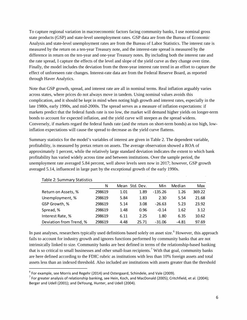
Summary statistics for the model’s variables of interest are given in Table 2. The dependent variable, profitability, is measured by pretax return on assets. The average observation showed a ROA of approximately 1 percent, while the relatively large standard deviation indicates the extent to which bank profitability has varied widely across time and between institutions. Over the sample period, the unemployment rate averaged 5.84 percent, well above levels seen now in 2017; however, GSP growth averaged 5.14, influenced in large part by the exceptional growth of the early 1990s.

In past analyses, researchers typically used definitions based solely on asset size.6 However, this approach fails to account for industry growth and ignores functions performed by community banks that are not intrinsically linked to size. Community banks are best defined in terms of the relationship-based banking that is so critical to small businesses and other small-loan recipients.7 With that goal, community banks are here defined according to the FDIC rubric as institutions with less than 10% foreign assets and total assets less than an indexed threshold. Also included are institutions with assets greater than the threshold 6 For example, see Morris and Regehr (2014) and Ostergaard, Schindele, and Vale (2009). 7 For greater analysis of relationship banking, see Hein, Koch, and MacDonald (2005); Critchfield, et al. (2004); Berger and Udell (2001); and DeYoung, Hunter, and Udell (2004).

Table 2: Summary StatisticsN Mean Std. Dev. Min Median Max

Return on Assets, % 298619 1.01 1.89 -135.26 1.26 369.22Unemployment, % 298619 5.84 1.83 2.30 5.54 21.68GSP Growth, % 298619 5.14 3.08 -26.63 5.23 23.92Spread, % 298619 1.48 0.96 -0.14 1.62 3.12Interest Rate, % 298619 6.11 2.25 1.80 6.35 10.62Deviation from Trend, % 298619 4.48 25.71 -31.06 -4.81 97.69

7

but with substantial loan-to-asset ratios, high core-deposit-to-assets ratios, and a limited geographical footprint.8 The sample covers all community banks from 1985 through 2015.

The attrition correction data are constructed from FDIC call reports. Call reports are collected on a quarterly basis and track information at the bank level, comprising all the bank-level characteristics used in this study. The data consist of 20,335 unique community banks, of which 6,175 remain in 2015 and 4,368 have observations for every sample year. These banks range from de novo charters to institutions that have operated for over 200 years. Over the 31-year period, 4,516 new banks enter the data set, and 14,249 banks permanently exit—while some of this attrition is due to bank failure, the vast majority of exit results from outgrowing the community bank definition, acquisition, or merger. Community banks in the sample tend to be relatively small, with the typical bank holding assets valued around $69 million and employing 28 employees. However, there are also included larger institutions, the largest of which have more than 10,000 employees and assets of more than $30 billion. Among these larger institutions, 443 banks fluctuate in size and complexity such that they lose and regain their community bank designation at least once over the time period. Bank characteristic summary statistics are reported in Table 3.

State-level variables were chosen as the best compromise between capturing macroeconomic forces and allowing for local variation. Data exist at the metropolitan statistical area and county levels; however, that level of geographic localization could prove problematic. It is reasonable to assume that community banks individually have no appreciable effect on national economic conditions. Furthermore, it is argued here that such banks have small enough impact on state-level economic conditions such that gross state product and unemployment may be considered exogenous to any given community bank’s performance. However, it is likely that at the county level, each community bank may have a significant impact on the county’s economic environment, leading to issues of endogeneity through simultaneity bias.

8 Threshold indexed to $250 million in 1985 and $ 1 billion in 2010. For more in-depth analysis of this functional definition of community bank, see FDIC (2012).

Table 3: Bank CharacteristicsMean Std. Dev. Min Median Max

Age 66 39 1 74 215Assets, million $ 159 339 0 69 30,984Deposits, million $ 132 266 0 60 25,468Equity, million $ 15 34 -1,093 6 2,758Liabilities, million $ 145 308 0 62 28,226Employees 53 88 1 28 10034

8

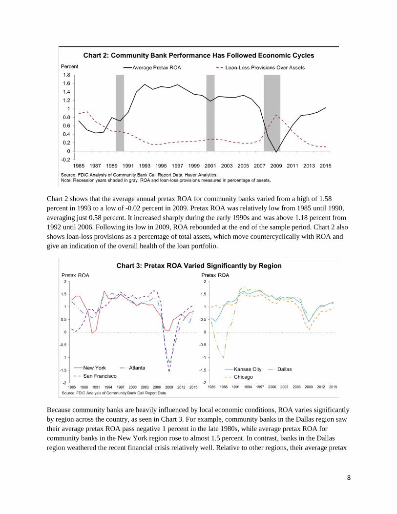
Chart 2 shows that the average annual pretax ROA for community banks varied from a high of 1.58 percent in 1993 to a low of -0.02 percent in 2009. Pretax ROA was relatively low from 1985 until 1990, averaging just 0.58 percent. It increased sharply during the early 1990s and was above 1.18 percent from 1992 until 2006. Following its low in 2009, ROA rebounded at the end of the sample period. Chart 2 also shows loan-loss provisions as a percentage of total assets, which move countercyclically with ROA and give an indication of the overall health of the loan portfolio.

Because community banks are heavily influenced by local economic conditions, ROA varies significantly by region across the country, as seen in Chart 3. For example, community banks in the Dallas region saw their average pretax ROA pass negative 1 percent in the late 1980s, while average pretax ROA for community banks in the New York region rose to almost 1.5 percent. In contrast, banks in the Dallas region weathered the recent financial crisis relatively well. Relative to other regions, their average pretax

9

ROA dipped only slightly to 0.62 percent, whereas at the same time the average pretax ROA of community banks in the San Francisco region fell sharply to almost negative 1.6 percent.

Results

Estimation finds that the five macroeconomic factors—economic growth, unemployment rate, interest-rate spread, interest rates, and deviations in interest-rate trend—together explain a significant part of the variation in pretax ROA across community banks. On average, macroeconomic factors accounted for more nearly two-thirds (66 percent) of the total variation in ROA; however, this fluctuated significantly over time. Structural industry factors explain nearly all of the observed deviation from the period average core ROA in the late 1980s, as macroeconomic factors played a negligible role in determining ROA for community banks during the S&L crisis. During the stronger, more economically stable years of the 1990s and early 2000s, macroeconomic factors explain 82 percent of the variation in ROA. Finally, since the financial crisis in 2008, the exceptionally weak post-crisis expansion account for approximately 80 percent of the variation in community bank.

Chart 4 shows the contributions of the five macroeconomic factors to pretax ROA over time. Together, the macroeconomic factors lowered pretax ROA by 2 basis points from 1985 to 1990; changes in structural factors were the primary forces affecting community bank ROA during the S&L crisis. Macroeconomic factors increased pretax ROA by 20 basis points from 1991 to 2007, peaking at 41 basis points in 1998. The effect of the crisis had a large negative impact, reducing pretax ROA by 85 basis points in 2009 and by 84 basis points in 2010. The drag from macroeconomic factors gradually declined as the post-recession recovery progressed, falling to a 31 point decrement in 2013 before finally reversing in 2015 to provide an 11 basis point boost.

The unemployment rate is the dominant macroeconomic factor affecting community bank ROA across the sample period. This is not surprising given that community banking is focused on local relationship-based lending: a strong local job market boosts demand for loans while a weak job market may raise delinquency rates. From 1995 to 2007, low unemployment boosted community bank ROA by an average of 32 basis points annually. Conversely, the sharp increase in unemployment during the financial crisis hit

10

hard, reducing pretax ROA by 74 basis points in 2009 and 76 basis points in 2010. The subsequent decline in unemployment first lessened the drag on community bank profitability. By 2014, low unemployment was a net contributor to bank profitability, and in 2015 the model predicts that it potentially added 28 basis points to industry ROA.

Gross state product growth is the least influential of the four macroeconomic factors. Local unemployment, interest rates, and interest-rate spreads affect community bank profitability directly, whereas economic growth affects banks indirectly—often through the channel of the other macroeconomic factors—likely explaining this result.

The interest rate generally had a relatively small impact on community bank profitability over the sample period, with the major exception of the post-crisis period in which the federal funds rate hit the zero lower bound. Over this period, the negative effect of interest rates grew from 11 basis points in 2009 to as much as 53 basis points in 2014. This lends credence to the oft-suggested theory that the longer interest rates remained exceptionally low, the more damaging they became to bank profitability. The corner was turned in 2015 when the Federal Open Market Committee raised rates above zero for the first time in 7 years.9

The impact of the interest-rate spread on community bank industry profitability is directly related to the size of the spread and generally moved independently of the other three macroeconomic variables. The spread had a small positive impact in the first two years, a negative impact when the yield curve inverted prior to the 1990 to 1991 recession, and a large positive impact when the yield curve steepened sharply in the first half of the 1990s. The spread again had a negative impact in the mid-1990s through the recession of 2001, when the yield curve flattened before inverting in 2000. In 1995 through 1998, the spread was the only macroeconomic factor that had a negative impact on profitability. The pattern repeated itself following the 2001 recession, with a steep yield curve boosting community bank profits before gradually flattening and finally inverting just before the 2008 financial crisis.

9 The FOMC’s action took place in December 2015. However, forward guidance and clear communication allowed the market to price in the interest rate lift-off well in advance.

11

Trends in Core Profitability

One explanation put forward for the decline in profitability among banks is the impact of new regulations put into place following the financial crisis. Among these are a range of regulations mandated by the Dodd-Frank Act of 2010 and the Basel III capital standards introduced in 2013; however, regulation is just one among many noneconomic factors that may contribute to structural change in community bank profitability. Other structural factors may include the rise of nonbank lending, competition from larger banks, and changes in loan portfolios and other business practices. Given that macroeconomic factors can account for 80 percent of the post-crisis variation in ROA, the net effect of structural factors combined explains the remaining 20 percent of post-crisis ROA variation.

Core profitability is the intrinsic earning capacity of a bank, after controlling for the impact of macroeconomic factors. It is a measure of the impact of structural factors on pretax ROA. Using the estimates from the model, it is possible to construct a counterfactual core ROA that estimates what community bank profitability would have been in the absence of any positive or negative economic shocks. Chart 5 shows that core ROA averaged 1.01 percent from 1985 through 2015. Core ROA and observed ROA generally evolve together, but core ROA is more stable with less variability around the average. Note that the difference between core ROA and observed ROA each year is the net effect of the model’s macroeconomic factors.

Core profitability among community banks was at its lowest during the S&L crisis of the late 1980s. It improved through the early 1990s, possibly as the competitive environment evolved following the failure of more than 1,700 banks and savings and loans, which eliminated many less-profitable institutions. After peaking in 1992, core profitability declined gradually over the following decade as a strong economy helped boost earnings, but enabled less profitable banks to operate. Bank responses to the recession of 2001 arrested this trend in core profitability for two years, after which core ROA resumed its downward trajectory. Core profitability reached its lowest level since the S&L crisis during the financial crisis in 2008, falling to 0.51 percent. The subsequent rapid-fire failure of 440 banks between 2009 and 2012, which eliminated many underperforming banks, combined with other structural changes to the

12

competitive environment to reverse the long-term downward trend and resulted in a marked upturn in core profitability.

Core profitability has been relatively strong throughout the post-crisis period, remaining at or above its historical average until 2015. The sharp decline in observed ROA during the financial crisis and subsequent recession is largely attributable to the severity of the downturn in macroeconomic factors, primarily the unemployment rate. At their extreme, macroeconomic factors reduced community bank profitability by 85 basis points in 2009. From 2010 onward, the slow pace of macroeconomic recovery and the persistence of historically low interest rates continued to be a drag on profitability, although by less in each successive year. By 2015, macroeconomic factors were no longer a headwind to ROA and in fact are estimated to have constituted a slight tailwind.

The Potential Effect of Entry and Exit on Core Profitability Trends

The number of community banks has fallen steadily from a high of 15,957 in 1985 to 5,874 at the end of the sample in 2015. One structural factor that is measureable and offers a potential explanation of trends observed in core profitability is entry and exit of community banks, which affects core ROA by changing the composition of community banks over time.10 New entries may increase competitive pressures on existing community banks and may lower overall core earning potential. Conversely, the failure or merger of less-productive banks may cause both observed ROA and core ROA to rise, as underperformers are removed from the sample.

Chart 6 shows that bank entry and exit correlate closely with overall trends in ROA: a rise in failures corresponds to an increase in core ROA (and observed ROA), whereas higher entry and fewer failures corresponds to a decline in core ROA. The rate of de novo entry follows a clear cyclical pattern—rising in expansions and falling in recessions—while the rate at which banks exit follows the opposite pattern. The period since the financial crisis in 2008 and subsequent recession is exceptional in that de novo charters have not increased as the economy has expanded.

During the S&L crisis period from 1985 to 1990, when entry rates were falling and failure rates were growing, core ROA rose at an average rate of 1.3 basis points per year. During the economically strong period from 1991 to 2007, when many banks entered and few banks failed, core ROA fell at an average rate of 1.5 basis points per year. Finally, during the financial crisis, recession, and subsequent economic recovery, the high rate of failures and lack of new charters corresponds to a strong upward trend in core ROA of 6.2 basis points per year.

10 The compositional effect from entry and exit is independent of any econometric bias introduced by entry and exit. Banks’ exiting the sample results in a measurement bias if the same unobserved factors that influence profitability also affect failure rates. This analysis uses a standard econometric technique to identify and correct for this bias: an F-test shows that the coefficient on the inverse Mills ratio—the attrition bias correction factor—is statistically significant, confirming the presence of attrition bias. Results suggests that if banks hadn’t outgrown the sample in the boom times, average ROA would have been up to 12 basis points higher in some years. Conversely, if banks hadn’t failed out of the sample during the recent crisis, in some years average ROA would have been 11 basis points lower.

13

The correlation between bank entry and exit and community bank core profitability is strong; however, this is not to suggest that compositional effects from entry and exit explain all of the variation in core profitability. Changes in other structural factors such as business practices, competitive environment, and regulation also play an important role; however, unlike entry and exit, these other structural factors are difficult to measure reliably.

Regional Analysis

As seen in Table 4, the regions differed significantly from one another in nearly all respects, reflecting the broad diversity expressed across community banks.

The New York region suffered a steep decline in pretax ROA during the 1990 recession, but weathered the recent crisis comparatively well. Interest rate fluctuations had a moderately stronger impact on the ROA of banks in this region, while the other factors had commensurately reduced effects. Core ROA for the region was much more stable than for the nation as a whole, with economic shocks accounting for most of the deviations from trend. Unfortunately, that trend has been a slow but unabated downward trajectory since the early 1990s, falling on average 1.4 basis points per year.

The Atlanta region was one of the hardest hit by the 2008 financial crisis, with regional average ROA plummeting to negative 1.2 percent. The region differs primarily from the national pattern in its sensitivity to gross state product shocks. In many years, the effects of economic growth exceeded the effects of unemployment—the only market in which this occurred. Core ROA broadly follows the national pattern by rising steeply in the late 1980s, falling gradually across the 1990s and 2000s, and finally rising again post-crisis; however, since 1989 regional average ROA has typically been 15 to 25 basis points lower than the national average.

Table 4: Regional Responses to Macroeconomic Fluctuations

14

The Chicago and Kansas City regions are largely a matched pair, perhaps explained by the high level of similarity within the states across the American Midwest in terms of economics and industry. The Chicago region expresses a slightly raised sensitivity to interest rate variation, compared with the Kansas City region, with this difference most prominent in the mid-1980s. Core ROA for both regions has been remarkably stable across the entire sample period, with averages of 1.09 and 1.22 for Chicago and Kansas City, respectively.

The Dallas region was the hardest hit by the S&L crisis of the late 1980s but was one of the strongest during the recent financial crisis, in a reversal of the Atlanta region’s experience. The S&L crisis saw regional community bank average ROA drop to -1.01 percent, after which it rebounded to 1.81 percent, the highest average ROA posted by any region in any sample year. The analysis indicates that the Dallas region’s community banks are the most sensitive to lagged values of interest rates and to deviations from interest rate trends, perhaps indicating a difference in the maturity composition of their loan portfolios. From 1991 onward, core profitability in the region expressed a generally gentle decline followed by an upturn after the financial crisis, falling by 1.9 basis points annually from 1991 to 2008, then rising 3.5 basis points annually thereafter.

During the financial crisis, community bank average ROA in the San Francisco region plummeted to negative 1.59 percent, lower than any other region in any year. However, the western U.S. states suffered

15

some of the worst employment shocks during the crisis, and this is reflected in the 74 basis points in ROA that the model predicts were lost due to job market disruption. While core profitability follows the national pattern for most of the sample, it appears to peak in 2013 and to go into a steep decline in the following two years, which may suggest greater stress in this region than in others around the country.

What Can We Conclude About Core Profitability Among Community Banks?

Understanding the evolution of core profitability among community banks requires an econometric approach that distinguishes the impact of macroeconomic factors from structural factors on observed profitability. This model estimates the impact of the macroeconomic factors on pretax ROA in order to net them out and arrive at a counterfactual core profitability measure that imagines a world free from macroeconomic shocks. This core profitability therefore represents the structural component of community bank profitability.

Analyzing a sample period from 1985 through 2015, this model indicates that core profitability rose sharply from a low in the late 1980s during the S&L crisis to a high in the early 1990s, trended down slowly through the mid-2000s before falling sharply to a low during the financial crisis in 2008, and then returned to pre-crisis levels during the weak economic recovery in the years following the financial crisis. The model finds that macroeconomic factors are largely responsible for the low level of community bank profitability during and after the financial crisis, and that core profitability generally has been at or above its long-run level since 2009. These findings suggest that the fundamental earnings model of community banks remains sound, despite the challenging post-crisis economic environment.

16

References

Achen, Christopher. 2001. “Why Lagged Dependent Variables Can Suppress the Explanatory Power of Other Independent Variables.” Working Paper 1001, University of Michigan.

Adams, Robert, and Jacob Gramlich. 2016. “Where Are All the New Banks? The Role of Regulatory Burden in New Bank Formation.” Review of Industrial Organization 48:181–208.

Albertazzi, Ugo, and Leonardo Gambacorta. 2009. “Bank Profitability and the Business Cycle.” Journal of Financial Stability 3:393–409.

Athanasoglou, Panayiotis, Sophocles Brissimis, and Matthaios Delis. 2006. “Bank-Specific, Industry-Specific and Macroeconomic Determinants of Bank Profitability.” Journal of International Financial Markets, Institutions, and Money 18:121–136.

Beckmann, Rainer. 2007. “Profitability of Western European Banking Systems: Panel Evidence on Structural and Cyclical Determinants.” Deutsche Bundesbank Discussion Paper, Series 2, No. 17/2007, Deutsche Bank.

Berger, Allen, and Gregory Udell. 2001. “Small Business Credit Availability and Relationship Lending: The Importance of Bank Organisational Structure.” Board of Governors of the Federal Reserve System, FEDS Working Paper No. 2001-36.

Bikker, Jacob, and Haixia Hu. 2002. “Cyclical Patterns in Profits, Provisioning and Lending of Banks and Procyclicality of the New Basel Capital Requirements.” BNL Quarterly Review 221:143–175.

Bureau of Labor Statistics, U.S. Department of Labor. 2015. “Local Area Unemployment Statistics.” November 17. www.bls.gov.

Bourke, Philip. 1989. “Concentration and Other Determinants of Bank Profitability in Europe, North America, and Australia.” Journal of Banking and Finance, 13:65–79.

Boyd, John, and Mark Gertler. “1993. U.S. Commercial Banking: Trends, Cycles, and Policy.” NBER Working Paper, No. 4404, National Bureau of Economic Research.

Critchfield, Tim, Tyler Davis, Lee Davison, Heather Gratton, George Hanc, and Katherine Samolyk. 2004. “Community Banks: Their Recent Past, Current Performance, and Future Prospects.” FDIC Banking Review 16:1–56.

Demirgüc-Kunt, Asli, and Harry Huizinga. 1999. “Determinants of Commercial Bank Interest Margins and Profitability: Some International Evidence.” The World Bank Economic Review 13:430–455.

DeYoung, Robert, and Karin Roland. 2001. “Product Mix and Earnings Volatility at Commercial Banks: Evidence From a Degree of Leverage Model.” Journal of Financial Intermediation 10:54–84.

DeYoung, Robert, William Hunter, and Gregory Udell. 2004. “The Past, Present and Probable Future of Community Banks.” Journal of Financial Services Research 25:85-133.

Ho, Thomas, and Anthony Saunders. 1981. “The Determinants of Bank Interest Margins: Theory and Empirical Evidence.” Journal of Financial and Quantitative Analysis, 16:581–600.

Hein, Scott, Timothy Koch, and S. Scott MacDonald. 2005. “On the Uniqueness of Community Banks.” Federal Reserve Bank of Atlanta Economic Review, 1:15–36.

Federal Deposit Insurance Corporation (FDIC). 2012. FDIC Community Banking Study. Washington, DC, FDIC.

17

Godard, John, Philip Molyneux, and John Wilson. 2004. “Dynamics of Growth and Profitability in Banking.” Journal of Money, Credit, and Banking. 16:1069–90.

Kanas, Aanglos, Dimitros Vasiliou, and Nikolaos Eriotis. 2012. “Revisiting Bank Profitability: A Semi-parametric Approach.” Journal of International Financial Markets, Institutions, and Money 22:990–1005.

Morris, Charles, and Kristen Regehr. 2014. “What Explains Low Net Interest Income at Community Banks?” Federal Reserve Bank of Kansas City Economic Review 2:59–87.

Molyneux, Philip, and John Thornton. 1992. “Determinants of European Bank Profitability.” Journal of Banking and Finance. 16:1173–1178.

Niepmann, Friederike. 2014. “Banking Across Borders with Heterogeneous Banks.” Staff Reports 609, Federal Reserve Bank of New York.

Ostergaard, Charlotte, Ibolya Schindele, and Bent Vale. 2009. “Social Capital and the Viability of Stakeholder-Oriented Firms: Evidence from Norwegian Savings Banks.” EFA 2009 Bergen Meetings Paper.

Petersen, Mitchell. 2009. “Estimating Standard Errors in Finance Panel Data Sets: Comparing Approaches.” Review of Financial Studies 22:435–480.

Tregenna, Fiona. 2009. “The Fat Years: The Structure and Profitability of the US Banking Sector in the Pre-crisis Period.” Cambridge Journal of Economics 33:609–632.

U.S. Bureau of Economic Analysis. 2015. “Annual Gross Domestic Product by State.” November 17. http://www.bea.gov/regional.

Vella, Francis. 1998. “Estimating Models with Sample Selection Bias: A Survey.” Journal of Human Resources 33 (1):127–169.

Wooldridge, Jeffrey. 2010. “Censored Data, Sample Selection, and Attrition.” In Econometric Analysis of Cross Section and Panel Data, 2nd ed., 837–845. Cambridge, MA: MIT Press.

18

Appendix: Attrition Correction

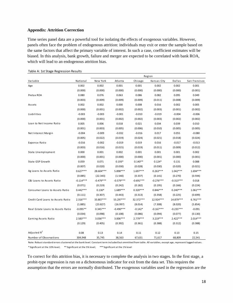
Time series panel data are a powerful tool for isolating the effects of exogenous variables. However, panels often face the problem of endogenous attrition: individuals may exit or enter the sample based on the same factors that affect the primary variable of interest. In such a case, coefficient estimates will be biased. In this analysis, bank growth, failure and merger are expected to be correlated with bank ROA, which will lead to an endogenous attrition bias.

To correct for this attrition bias, it is necessary to complete the analysis in two stages. In the first stage, a probit-type regression is run on a dichotomous indicator for exit from the data set. This requires the assumption that the errors are normally distributed. The exogenous variables used in the regression are the

Table A: 1st Stage Regression Results

Variable National New York Atlanta Chicago Kansas Ci ty Dal las San Francisco

Age 0.002 0.002 0.001 0.001 0.002 0.002 0.001

(0.000) (0.000) (0.000) (0.000) (0.000) (0.000) (0.001)

Pretax ROA 0.080 0.076 0.063 0.086 0.082 0.095 0.049

(0.003) (0.009) (0.009) (0.009) (0.011) (0.008) (0.009)

Assets 0.002 0.002 0.000 0.008 0.016 0.002 0.005

(0.000) (0.001) (0.002) (0.002) (0.003) (0.001) (0.002)

Liabi l i ties -0.003 -0.003 -0.001 -0.010 -0.019 -0.004 -0.006

(0.000) (0.001) (0.002) (0.002) (0.003) (0.002) (0.002)

Loan to Net Income Ratio 0.005 0.006 0.018 0.021 0.034 0.039 0.010

(0.001) (0.003) (0.005) (0.006) (0.010) (0.005) (0.005)

Net Interest Margin -0.004 -0.009 -0.032 -0.016 0.017 0.055 -0.080

(0.005) (0.022) (0.019) (0.024) (0.021) (0.018) (0.024)

Expense Ratio -0.016 -0.002 -0.019 0.019 0.016 -0.017 -0.013

(0.003) (0.016) (0.015) (0.019) (0.011) (0.009) (0.012)

State Unemployment 0.000 0.001 0.002 0.001 0.001 0.001 0.002

(0.000) (0.001) (0.000) (0.000) (0.001) (0.000) (0.001)

State GSP Growth 0.059 0.071 0.193* 0.140** 0.124* 0.131 0.088

(0.007) (0.020) (0.030) (0.028) (0.030) (0.020) (0.021)

Ag Loans to Assets Ratio 0.627*** 28.604*** 5.898*** 1.697*** 0.263*** 1.042*** 1.694***

(0.085) (22.343) (1.540) (0.337) (0.141) (0.270) (0.594)

C&I Loans to Assets Ratio -0.114*** -0.479*** -0.579*** -0.691*** -0.276*** -0.313*** 0.018

(0.071) (0.219) (0.242) (0.182) (0.195) (0.166) (0.224)

Consumer Loans to Assets Ratio 0.442*** 0.130* 1.689*** 0.320*** 0.846*** 0.240*** 1.061***

(0.111) (0.307) (0.443) (0.313) (0.358) (0.225) (0.699)

Credit Card Loans to Assets Ratio 2.316*** 33.807*** 55.297*** 32.372*** 12.924*** 14.879*** 6.761***

(1.885) (23.827) (16.997) (8.014) (7.308) (8.020) (5.854)

Real Es tate Loans to Assets Ratio -0.095** 0.345*** -0.490*** -0.142* -0.167*** -0.235*** -0.091

(0.034) (0.098) (0.108) (0.086) (0.094) (0.077) (0.130)

Earning Assets Ratio 2.583*** 3.036*** 3.006*** 2.779*** 3.219*** 2.422*** 2.014***

(0.129) (0.405) (0.392) (0.361) (0.388) (0.312) (0.388)

Adjusted R2 0.08 0.13 0.14 0.11 0.12 0.13 0.15

Number of Observations 304,948 35,745 38,563 67,631 71,617 68,809 22,541

* Significant at the 10% level; ** Significant at the 5% level; *** Significant at the 1% level

Region

Note: Robust standard errors clustered at the bank level. Constant term included but ommitted from table. All variables, except age, represent lagged values.

19

lagged values of various bank-level factors. A separate regression is run for each time period, effectively transforming the data from time series to cross section. The inverse Mill’s ratio from each cross-sectional regression is calculated and the results are tabulated as a vector for use in the second-stage regression. Results from the first-stage regression are shown in Table A.

While the magnitude and significance of the regressors in this first stage are not of particular importance to the main analysis, it is interesting to note that many characteristics that might commonly be assumed to be strong predictors of bank success or failure are here found to be not significant. These include the net interest margin, pretax ROA, assets, and liabilities. In contrast, the loan portfolio variables, listed as asset ratios, were generally highly significant.

The first-stage probit regressions generate pseudo r-squared values ranging from a high of 0.433 to a low of 0.02. The mean pseudo r-squared values for each region are reported in Table A.