core.ac.uk · supervisors docent luigia petre department of information ecthnologies Åbo akademi...
TRANSCRIPT

Turku Centre for Computer Science
TUCS DissertationsNo 162, September 2013
Maryam Kamali
Reusable Formal Architectures for Networked Systems


Reusable Formal Architectures forNetworked Systems
Maryam Kamali
To be presented, with the permission of the Department of InformationTechnologies at Åbo Akademi University, for public criticism in Auditorium
Gamma on September 13, 2013, at 12 noon.
Turku Centre for Computer ScienceÅbo Akademi University
Department of Information TechnologiesJoukahainengatan 3-5, 20520 Åbo, Finland
2013

Supervisors
Docent Luigia PetreDepartment of Information TechnologiesÅbo Akademi UniversityJoukahaisenkatu 3-5, 20520, TurkuFinland
Professor Kaisa SereDepartment of Information TechnologiesÅbo Akademi UniversityJoukahaisenkatu 3-5 A, 20520, TurkuFinland
Reviewers
Professor Tiziana Margaria-Ste�enInstitute for InformaticsUniversity of PotsdamAugust Bebel Straÿe 89, 14482, PotsdamGermany
Doctor Helen TreharneDepartment of ComputingUniversity of SurreyGuildford, Surrey, GU2 7XHUK
Opponent
Professor Tiziana Margaria-Ste�enInstitute for InformaticsUniversity of PotsdamAugust Bebel Straÿe 89, 14482, PotsdamGermany
ISBN 978-952-12-2932-9ISSN 1239-1883

To my mom and dad
تقدیمع بع پدرع وع مادع عزی�م

ii
Abstract
Today's networked systems are becoming increasingly complex and diverse.The current simulation and runtime veri�cation techniques do not providesupport for developing such systems e�ciently; moreover, the reliability ofthe simulated/veri�ed systems is not thoroughly ensured. To address thesechallenges, the use of formal techniques to reason about network system de-velopment is growing, while at the same time, the mathematical backgroundnecessary for using formal techniques is a barrier for network designers toe�ciently employ them. Thus, these techniques are not vastly used for de-veloping networked systems.
The objective of this thesis is to propose formal approaches for the deve-lopment of reliable networked systems, by taking e�ciency into account.With respect to reliability, we propose the architectural development ofcorrect-by-construction networked system models. With respect to e�ciency,we propose reusable network architectures as well as network development.At the core of our development methodology, we employ the abstractionand re�nement techniques for the development and analysis of networkedsystems. We evaluate our proposal by employing the proposed architectu-res to a pervasive class of dynamic networks, i.e., wireless sensor networkarchitectures as well as to a pervasive class of static networks, i.e., network-on-chip architectures. The ultimate goal of our research is to put forwardthe idea of building libraries of pre-proved rules for the e�cient modelling,development, and analysis of networked systems. We take into account bothqualitative and quantitative analysis of networks via varied formal tool sup-port, using a theorem prover � the Rodin platform � and a statistical modelchecker � the SMC-Uppaal.
iii

iv

Sammanfattning
Nätverkssystem blir numera allt mer invecklade och olika varandra. De ex-isterande teknikerna för simulering och körtidsveri�ering ger inget stöd före�ektiv utveckling av nätverkssystem, och utöver detta kan simulerade/ ve-ri�erade systems pålitlighet inte fullständigt garanteras. För att möta dessautmaningar har användningen av formella metoder för att resonera kring ut-veckling av nätverkssystem ökat, men den matematiska bakgrund som krävsför att använda formella metoder hindrar samtidigt nätverksutvecklare frånatt e�ektivt dra nytta av dessa metoder. För utveckling av nätverkssystemanvänds dessa metoder därför inte i någon större utsträckning.
Målsättningen med denna avhandling är att föreslå formella tillväga-gångssätt för utveckling av pålitliga nätverkssystem där e�ektiviteten tasi beaktande. Gällande pålitligheten föreslår vi modeller av nätverkssystemvars arkitektur utvecklas korrekt genom konstruktionen. När det gäller e�ek-tivitet föreslår vi nätverksarkitekturer och nätverksutveckling som kan åter-användas. Kärnan i vår utvecklingsmetodologi är att använda abstraktion-och preciseringstekniker för utveckling och analys av nätverkssystem. Vi ut-värderar vårt förslag genom att använda de föreslagna arkitekturerna för engenomgripande klass av dynamiska nätverk, det vill säga trådlösa sensornät-verk, och likaså en genomgripande klass av statiska nätverk, det vill sägaarkitekturer för nätverk-på-chip. Det slutgiltiga målet med vår forskning äratt föra fram idén om att bygga bibliotek innehållande på förhand bevisa-de regler för e�ektiv modellering, utveckling och analys av nätverkssystem.Vi tar i beaktande såväl kvalitativ som kvantitativ analys av nätverk viaolika formella verktyg såsom Rodin-plattformen, för bevis av teorem, ochSMC-Uppaal, för statistisk modellkontroll.
v

vi

Acknowledgements
First of all, I would like to express profound thanks to my supervisors DocentLuigia Petre and Prof. Kaisa Sere for their excellent advice and support, fortheir continuous encouragement, for the countless scienti�c discussions wehave had, and for always being there to help, no matter the time or date.Furthermore, I wish to thank Prof. Tiziana Margaria-Ste�en and Dr. HelenTreharne for their valuable reviews of this dissertation and for providingconstructive comments that improved its quality. Particular thanks are dueto Prof. Tiziana Margaria-Ste�en for also agreeing to act as an opponent atthe public defence of the thesis.
I am grateful to all the members of the Department of Information Tech-nologies at Åbo Akademi University, especially my colleagues at the Dis-tributed Systems Laboratory and Turku Centre for Computer Science forproviding such a friendly atmosphere to work. In particular, I wish to thankDocent Linas Laibinis for his advice and encouragement as well as Dr. An-ton Tarasyuk, Dr. Mats Neovius and Petter Sandvik for their help withpractical matters and the Swedish version of the abstract. I would like toacknowledge Prof. Ansgar Fehnker's kind help and supervision during mystay at University of the South Paci�c, Fiji. I extend my sincere thanks toDr. Peter Höfner, Prof. Rob J. van Glabeek and Prof. Frank Cessar fortheir supervision and friendship during my stay at NICTA, Australia. I amvery grateful to all my co-authors for the knowledge they shared with me.
I gratefully thank the Turku Centre for Computer Science and the De-partment of Information Technologies at Åbo Akademi University for thegenerous funding of my doctoral studies and travels. I would like to alsoacknowledge the Nokia foundation and the Ulla Tuomienen Foundation forgranting me research scholarships that supported my work.
Finally, I would like to express my thankfulness to my family and myfriends for their cheeriness and support throughout these years. I am es-pecially grateful to my brothers, Ehsan and Morteza, and my dear sister,Mojgan, who continuously motivated me to keep the pace in my research.I would like to express my deepest gratitude to my dearest parents, Nahidand Ali, for their love and support during di�erent phases of my life. Thisdissertation is dedicated to you.
Maryam KamaliÅbo, August 2013
vii

viii

List of original publications
I Maryam Kamali, Linas Laibinis, Luigia Petre, and Kaisa Sere. FormalDevelopment of Wireless Sensor-Actor Networks, In Science of Com-puter Programming (SCP) Journal. Elsevier, 2012. DOI: 10.1016/j.scico.2012.03.002.
II Maryam Kamali, Linas Laibinis, Luigia Petre, and Kaisa Sere. A Dis-tributed Implementation of a Network Recovery Algorithm, In Interna-tional Journal of Critical Computer-Based Systems (IJCCBS), Vol. 4,No. 1, pp. 45-68. Inderscience Publishers, 2013.
III Ansgar Fehnker, Peter Höfner, Maryam Kamali, and Vinay Mehta.Topology-based Mobility Model for Wireless Networks, In K. Joshi etal. (Eds.) Proceedings of the 10th International Conference on Quan-titative Evaluation of Systems conference - QEST 13, Lecture Notes inComputer Science Vol. 8054, pp. 389-404, Springer-Verlag, 2013.
IV Peter Höfner, and Maryam Kamali. Quantitative Analysis of AODVand its Variants on Dynamic Topologies using Statistical Model Check-ing, In V. Braberman and L. Fribourg (Eds.) Proceedings of the 11thInternational Conference on Formal Modeling and Analysis of TimedSystems - FORMATS 13, Lecture Notes in Computer Science Vol. 8053,pp. 121-136, Springer-Verlag, 2013.
V Maryam Kamali, Luigia Petre, Kaisa Sere, and Masoud Daneshtalab.Re�nement-Based Modeling of 3D NoCs, In F. Arbab and M. Sirjani(Eds.) Proceedings of the 4th IPM International Conference on Funda-mentals of Software Engineering - FSEN 11, Lecture Notes in ComputerScience Vol. 7141, pp. 236-252, Springer-Verlag, 2012.
VI Maryam Kamali, Luigia Petre, Kaisa Sere, and Masoud Daneshtalab.Formal Modeling of Multicast Communication in 3D NoCs. In P. Kitsosand S. Niar (Eds.) Proceedings of the 14th Euromicro Conference onDigital System Design - DSD 2011, pp. 634-642. IEEE/Euromicro,August 2011.
ix
VII Maryam Kamali, Luigia Petre, Kaisa Sere, and Masoud Daneshtalab.CorreComm: A Formal Hierarchical Framework for Communication De-signs, In Proceedings of the 2nd IEEE International Conference on Net-worked Embedded Systems for Enterprise Applications - NESEA2011,pp. 1-7. IEEE Computer Society, December, 2011.
VIII Maryam Kamali, Luigia Petre, and Kaisa Sere. NetCorre: A Hierarchi-cal Framework and Theory for Network Design (Submitted to Science ofComputer Programming Journal), April, 2013.
x
Contents
Part I: Research Summary 1
1 Introduction 3
2 Networking Architectures 5
2.1 Dynamic Networks . . . . . . . . . . . . . . . . . . . . . . . . 62.2 Static Networks . . . . . . . . . . . . . . . . . . . . . . . . . . 8
3 Formal Methods 11
3.1 Event-B . . . . . . . . . . . . . . . . . . . . . . . . . . . . . . 133.2 Statistical Model Checking in Uppaal . . . . . . . . . . . . . . 16
4 Reusable Formal Network Architectures 19
4.1 Reusable and correct-by-construction WSANs . . . . . . . . . 194.2 Towards a reusable implementation of WSANs . . . . . . . . 204.3 A reusable mobility model for analysing ad-hoc networks . . . 204.4 Quantitative analysis of routing in ad-hoc networks . . . . . . 214.5 Reusable and correct-by-construction NoC architectures . . . 214.6 Reusable and correct-by-construction multicast routing in NoC
architectures . . . . . . . . . . . . . . . . . . . . . . . . . . . 224.7 A correct-by-construction framework for developing static net-
work architectures . . . . . . . . . . . . . . . . . . . . . . . . 224.8 A reusable and correct-by-construction network theory . . . . 23
5 Related Approaches 25
5.1 Modelling and Analysing Dynamic Networks . . . . . . . . . . 255.2 Modelling and Analysing Static Networks . . . . . . . . . . . 265.3 Architectural Development of Networked Systems . . . . . . . 275.4 Correct-by-Construction System Development . . . . . . . . . 29
6 Discussion 31
7 Bibliography 35
xi

Complete List of Publications 43
Pat II: Original Publications 45
xii
Part I
Research Summary
1


1. Introduction
In recent years, novel networked systems have increasingly emerged at bothlarge and small scale, such as wireless sensor networks, mobile ad-hoc net-works, networks-on-chip, etc. These networked systems are uniquely de-signed and implemented, according to their speci�c principles. For instance,the design of wireless sensor networks is derived mostly by considering thepower consumption, the data-centric nature of the sensor network, the nodecoordination techniques and the node failures. The design focus in mobilead-hoc networks is on mobility, spatial correlation, in-network data miningand link failures. Networks-on-chip are designed to address on-chip commu-nication issues and to provide for more e�cient embedded systems.
The proliferation of these and other novel network paradigms leads to re-thinking how to develop them in an e�cient as well as reliable way. E�cientdevelopment allows one to manage the complexity of networked systems andshorten their development time. Producing reliable systems means that wecan trust the developed system to behave according to its speci�cation.
The overall goal of this thesis consists in contributing to the developmentof networking architectures for e�ciency and reliability. This is a very largeand diverse area of research whose impact can be enormous, due to theubiquity of networked systems in our society. With respect to developinge�cient network architectures, we focus on the reusability of our proposedmodels. With respect to developing reliable network architectures, we studythe development of correct models from their speci�cations.
Our research method consists in applying formal methods toward achiev-ing our research goal. Formal methods aim at increasing the rigour of thedesign and of the development of systems by employing mathematical-basedtechniques used for speci�cation, development and veri�cation of systemmodels. Ultimately, formal methods aim at establishing software and sys-tem development as a discipline comparable to other engineering disciplinessuch as car manufacturing, avionics, construction and architecture, etc.
Networks can be classi�ed with respect to several criteria, such as themedium used for transporting data, the scale, the topology, etc. With re-spect to the medium used for communication, we distinguish between wirednetworks, where waves are transmitted along a physical medium such as a
3

twisted pair cable or an optical �ber and wireless networks, where microwave,radio or infrared waves are propagated through air. With respect to scale,we distinguish between local area networks (LAN), that connect devices overa relatively short distance and wide area networks (WAN) that span a largephysical distance. Network topology can be de�ned as the physical layoutof the interconnections and the devices in a network. Such a topology canbe dynamic when the layout evolves. A topology can also be static whenthe layout is �xed and unchangeable; in this case, we can distinguish be-tween bus, star, ring and mesh topologies. In our research we focus on thetopology taxonomy of networked systems, studying both static and dynamicnetworks. One reason for this choice is that it underlies both their functionaland non-functional properties.
Thus, we propose reusable formal architectures for networked systemsthat can be applied to both dynamic and static networks. We evaluate ourproposal by employing the proposed architectures to a pervasive class ofdynamic networks, i.e., wireless sensor network architectures as well as to apervasive class of static networks, i.e., network-on-chip architectures.
A complementary aspect of our work consists in developing systematicapproaches for both qualitative and quantitative analysis of these networks.We employ two main modelling and analysis frameworks: a theorem proverand a statistical model checker. The study focus in qualitative analysis ison designing correctly functioning networks, while in quantitative analysisthe study focus is on evaluating non-functional network properties such asperformance.
Our research is based on a collection of eight papers. We split this dis-sertation in two parts. In Part I we present the context and overall view ofthe work, while in Part II we reprint the research papers (with permission).In Part I we proceed as follows. In Section 2, we describe our object ofstudy, namely, our approach to networking architectures. In Section 3, wemotivate and overview the research methods we employ. In Section 4, weput everything together and explain how we apply the methods describedin Section 3 to the architectures described in Section 2; paper by paper, wecharacterise our contribution to the reusability and correctness of the devel-oped networked architectures, emphasizing the qualitative or quantitativeanalysis that we perform. In Section 5, we discuss related approaches to thisdissertation and in Section 6 we summarise our work as well as emphasizefuture research directions.
4

2. Networking Architectures
In this section we describe the design space of networked systems that iscovered in our study. We point out the main aspects of networks that aretaken into account in our architectural development.
A network consists of a set of interconnected devices that communicatewith each other via messages. Three central features are at the core of everynetworked system: the network topology, the resource management and therouting algorithm. In this dissertation we refer to a networking architectureas a set of these three features.
The network topology determines the physical layout of the devices andof their interconnections in the network. A network topology can be de�nedas a graph G = (V,E). The set of vertices V = {v1, v2, ..., vn} modelsthe network devices, called nodes. The set of edges E = {e1, e2, ...., em}models the interconnections, called links between the nodes; an edge ei,i ∈ {1, ...,m} is expressed as a pair of vertices (vj , vk), where vj , vk ∈ V . Theresource management refers to the usage of the edges and vertices of G forthe functioning of the network. A central concept for network functioningis that of a message. A message is a communication unit in a networkand is typically characterized by a source node, one or more destinationnodes, as well as some data. A routing algorithm determines the paths(also called routes) through the network, that messages take to reach theirdestinations. Routing algorithms can be classi�ed into several categories, forinstance adaptive or deterministic and unicast or multicast routing. In anadaptive routing algorithm, a path from a particular source to a destinationis determined when it is required, by considering the network state. In adeterministic routing algorithm, the routes of the messages to destinationsare determined at the initialization of the network; messages are alwaysrouted on a �xed path between a particular source and destination. Adaptiverouting algorithms are preferable in networks with frequent topology changesand non-uniform network tra�c: a better route might always be found in anew con�guration. Deterministic routing algorithms are e�cient in networkswith relatively stable topologies and regular tra�c patterns: they can safelyreuse already established routes. A unicast or multicast routing algorithmrefers to the message delivery scheme in networked systems. In the unicast
5

category, a message is delivered to a single speci�c destination node, whilein the multicast category, the same message is sent to a set of destinationnodes.
In this dissertation, our goal is to model, develop, and analyse reliablenetworking architectures for reusability. Our starting point consists of a veryabstract representation of a network topology - the graph G above -, that isassociated with abstract resource management and routing. Already in thisabstract view, two networking architectures can be derived: (i) a networkmodel with a varying set of nodes and interconnections and (ii) a networkmodel with a �xed set of nodes and interconnections. We refer to the models(i) for networking architectures as dynamic networks and to the models (ii)for networking architectures as static networks.
Modelling, developing and analysing networking architectures is highlyin�uenced by the network type. For this reason, in the following we put for-ward the most important issues concerning topology, resource management,and routing algorithms with respect to dynamic and static networks.
2.1 Dynamic Networks
The main concern in a dynamic network is to achieve its desired function-ality while the network topology frequently changes. The network topologychanges due to node or link failures. The node failure can happen at anytime due to unpredictable changes in the network, such as malfunctioning,shortage of power, etc. The link failures usually happen when nodes aremobile and move out of the range of their neighbours.
Network topology According to the two types of failures, we study twoessential features in our dynamic network topologies: unpredictable changesand mobility. The dynamic topology keeps changing with time and thus, wecan consider the network goes through a series of transition points ti, fori > 0. A transition point ti corresponds to a particular moment when thenetwork topology changes from Gi = (Vi, Ei) to Gi+1 = (Vi+1, Ei+1).
We specify the behaviour of the network topology in the presence ofunpredictable changes in the network with the following three sets of changesfor a transition point ti:
add_edges(i) =
{Vi+1 = Vi
Ei+1 = Ei ∪ {α}, α /∈ Ei
6

add_vertices(i) =
{Vi+1 = Vi ∪ {m}, m /∈ Vi
Ei+1 = Ei
delete_vertices(i) =
{Vi+1 = Vi \ {m}, m ∈ Vi
Ei+1 = Ei \ {γ}, γ = {(a, b) | a = m ∨ b = m}
These changes model the following situations. When a new link between twoneighbour nodes modelled by vertices m and k is discovered in the network,the corresponding edge α = (m, k) is added to the set of edges and theset of vertices does not change (add_edges(i)). Nodes can be added at anytime to a dynamic network, leading to a change in the set of vertices ofthe network graph, as described by add_vertices(i). When a node (e.g.,modelled by vertex m) fails, its corresponding vertex is deleted from the setof vertices. As a result, all its edges γ are also deleted from the set of edges(delete_vertices(i)).
We specify the behaviour of the network topology in the presence ofmobility with the following two sets of changes for a transition point ti:
add_edges(i) =
{Vi+1 = Vi
Ei+1 = Ei ∪ {α}, α /∈ Ei
delete_edges(i) =
{Vi+1 = Vi
Ei+1 = Ei \ {α}, α ∈ Ei
When a mobile node modelled by say, vertex m, enters the transmissionrange of another node, modelled by say, vertex k, the edge α = (m, k)corresponding to a link between vertices m and k is added to the set of edgesof the network graph; the set of vertices does not change (add_edges(i)).When a mobile node modelled by say, vertex m, leaves the range of one ofits neighbours modelled by say, vertex k, the edge α = (m, k) is deleted fromthe set of edges and the set of vertices does not change (delete_edges(i)).
Resource management In dynamic networks, nodes are untethered au-tonomous devices with power limitations due to their device types. Variousdevice types result in correspondingly various resources with their speci�ccomputation abilities and communication ranges. For instance, some morepowerful nodes may route messages from more limited nodes and some nodesmay act as gateways to long-range data communication networks. The de-gree of heterogeneity in dynamic networked systems is an important factora�ecting the resource management.
7
To address resource management features in dynamic networks, we havestudied two di�erent types of nodes together with their relationships. Con-sidering heterogeneity in a networked system design provides the means tomodel and analyse connectivity at di�erent levels. We have speci�ed thebehaviour of the network at three di�erent levels, based on three connectiv-ity graphs. Two of these graphs model the homogeneous interconnections,between nodes of the same type. The third graph models the heterogeneousinterconnections, between nodes of di�erent types.
Routing algorithm In order to discover routes in dynamic networks, thenetwork should be connected, i.e., there should always be a path, possi-bly over multiple hops, between any two nodes. However, due to topologychanges, the network may transform into a set of sub-networks disconnectedfrom each other; this set is called a network partition. In particular, thismeans that there can be nodes in the network that have no connection andmessages cannot be transported between them. A recovery mechanism isnecessary in this case, to re-establish connections between the sub-networks.The recovery should guarantee the establishment of connection between thesub-networks. We address the connectivity issue in our dynamic networkarchitecture by discovering a sub-graph of the network topology graph de-noting alternative links between separated sub-networks.
Apart from connectivity, route discovery and maintenance play a cru-cial role in the reliability and the performance of dynamic networks. TheAd Hoc On-Demand Distance Vector Routing protocol (AODV) [56] is ane�cient routing algorithm with di�erent variants, aimed at improving theperformance of dynamic networks. To reason about AODV and its vari-ants in dynamic networks, we use a dynamic topology model that considersmobility.
2.2 Static Networks
Static networks have a �xed set of nodes and interconnections. The mainconcern in a static network is to function predictably, i.e., according to agiven speci�cation. Hence, one important area of study is how to design andreason about various given speci�cations for network functioning.
Network topology The main characteristic of a static network consistsin its predictability. With respect to the network topology, this means thatwe can specify and reuse various topologies. In particular, we can developa hierarchy of static network topologies, where the most abstract one de-�nes concepts common to all network topologies. Such abstract topologyis essentially made of the graph G = (V,E) with the vertices V and the
8

corresponding edges E between vertices not evolving in time. We then spe-cialize this graph into a very common topology for static networks, namelythe mesh topology. The mesh topology is a regular graph structure thatmakes analysis of static networks possible. In a mesh topology, nodes can belaid out to form a 2-dimensional (2D) rectangular grid in which each nodeis connected to its four neighbours except for the nodes of the boundary.We specify the topology graph of a 2D mesh network for a �xed number ofnodes, say | V |= N . In such a mesh topology, we have a
√N ×√N mesh
structure, and the number of edges is less or equal than 2N : | E |≤ 2N . Theconnectivity degree du of a node u stores the number of pairs (v, u) ∈ E,for any v ∈ V ; du is also an important factor in the topology of a staticnetwork. For a 2D mesh network, we have that du ∈ [2, 4] for any u ∈ V .We can of course specialize the abstract topology to a n-dimensional (nD)mesh topology. For n = 3 (a 3-dimensional (3D) mesh topology) a �xed setof nodes N (| V |= N), we have a
√N × √N × √N mesh structure with
| E |≤ 3N and the connectivity degree du is so that du ∈ [3, 6] for any u ∈ V .
Resource management To analyse a systematic and e�ective architec-ture for static networks, apart from the message resource, other resourcessuch as channels and bu�ers should be managed. A message, which is gen-erated by a node, is further divided into packets and a packet can be furthersplit into a number of �its. A channel is a link that connects nodes together.In fact, channels are instantiations of edges in the network topology, allowingto model more network characteristics. A bu�er stores messages temporarilyin the start and end nodes of the channels. Moreover, in order to manageallocating bu�ers and channels to messages, we need to de�ne the switchingmechanism that determines how the message moves along the network path.Regarding the switching mechanism, bu�ers and channels can be allocatedto either messages, packets or �its. In message-based switching, channelsand bu�ers between a source and a destination across multiple hops are al-located to the whole message. In packet-based switching, the allocation ofchannels and bu�ers is handled independently for each packet. In �it-basedswitching, also called wormhole, �its of a packet follow each other and thesame set of channels and bu�ers are allocated to each individual �it of apacket, at di�erent moments.
We model and analyse the channel and bu�er structural elements ofa static network as well as messages, packets and �its in our architecturefor static networks. We also address switching techniques, to manage theallocation of channels and bu�ers at the message, packet and �it level.
Routing algorithm In static networks the issues in designing routing al-gorithms are to provide high throughput and low latency, and also to be
9

deadlock free. There are many routing algorithms that are proposed forvarious topologies of static networks ranging from adaptive to deterministicrouting schemes, to provide e�ciency in the presence of di�erent conges-tion conditions. In adaptive routing techniques in static networks, the routedecision is taken in each node, with respect to network tra�c. In deter-ministic routing techniques, the minimal route is typically chosen. As thenetwork topology does not change, nodes always route messages on the samepath. Therefore, the behaviour of nodes is di�erent in a static network withadaptive or deterministic routing algorithms. Moreover, in networks withunicast routing technique, nodes only need to route a message to one out-going channel. In networks with a multicast routing algorithm, nodes needto take decisions about routing a message on one or more outgoing chan-nels. In order to address di�erent characteristics of routing algorithms atthe architectural level, we model a hierarchy of fundamental architecturalcomponents and analyse them at di�erent levels of abstraction.
10

3. Formal Methods
In this section we describe the formal tools that we employ throughout thethesis. Formal methods can be seen nowadays as a contribution of computerscientists to raise software and software-intensive system development toan engineering level comparable to well established disciplines such as carmanufacturing, avionics, construction and architecture, etc.
One essential artefact common to these engineering disciplines is thatof blueprint or model. A model allows us to address the complexity of thesystem under development by abstraction, i.e., illustrating only the featuresof interest with respect to a particular model's purpose.
In model-driven development, �rst a high-level model of a system is devel-oped (often via numerous steps) and then the model is developed into a spec-i�cation closer to the implementation of the system. This development canconsist of adding details and functionalities and removing non-determinismand is typically referred to as re�nement [20]. The concepts of abstractionand re�nement are at the core of such a stepwise development. Abstractionis an essential feature for reusability. The abstract speci�cation typicallydescribes what the system does, whereas the more concrete speci�cationsderived by re�nement describe how it is done. In fact, the architecture ofa system is introduced in a high-level speci�cation and the design decisionsare gradually introduced in low-level speci�cations.
Formal methods are broadly divided into state-based and event-based,corresponding to the �rst class entities in the models. State-based methodsdeal with specifying systems by variables and operations that modify thesevariables. The values of the variables describe the state of the system. ActionSystems [16], the Z notation [63], the B-method [9], VDM [53] and Event-B [10] are all examples of state-based formal methods. Event-based formalmethods focus on representing systems by a composition of processes thatcommunicate via channels. Well-known examples of event-based methodsare CSP [39], CCS [49] and π-calculus [50]. A combination of state-basedand event-based methods are also proposed as CSP||B [59] and CSP||Event-B[60].
Nowadays, tool support is an essential instrument for the usability of aformal method. One reason for this is that tools provide a platform to cope
11
with system modelling and analysis at the same time; this promotes thee�cient use of formal methods. Another reason is that tools have features forsyntax checking and also, at some levels, they can automatically prove trivialproperties of a desired system. According to their type, tools associated toformal methods can be theorem provers, model checkers and simulators. Inthis dissertation, we employ the state-based formal method Event-B thathas an associated theorem prover tool, namely the Rodin platform [7, 12].We also �nd instrumental the event-based formalism of timed-automata [13],supported by tools such as the Uppaal [21] model checker and its statisticalextension called SMC-Uppaal [28].
Common to all formal methods is the concept of a precise (or formal)model. This essentially means that we can associate a meaning to the model,called semantics. Semantics can be de�ned as a mapping from a novel con-cept to a concept that we already understand well. Capturing a system atseveral levels of abstraction via formal models allows for two types of activ-ities that are speci�c to formal methods: formal development and analysisof various properties.
Event-B combines the idea of model-driven development and formal meth-ods to construct a correct model of a system. In this framework, a formalabstract model of a system with its desired properties is speci�ed and provedcorrect with respect to its speci�cation. The high-level speci�cation is thendeveloped at several di�erent re�nement levels. The notion of re�nement ismathematically de�ned in Event-B in a way that allows us to analyse therelationship between formal speci�cations at di�erent levels of abstraction.This corresponds to a qualitative analysis of the system.
In Event-B, in each re�nement step, certain design decisions are intro-duced into the system speci�cation. There might be various design alterna-tives that can provide the desired functionality with distinct consequencesfor the non-functional properties of the system. In order to choose the opti-mal design alternative, a quantitative analysis of non-functional properties,(e.g., performance) should also be undertaken.
To assess system performance in a networked system, the probabilitythat a system correctly functions over a given period of time should be eval-uated. To achieve quantitative assessment in networked systems, we use anextension of timed-automata in Uppaal for system speci�cation, called pricetimed-automata; this integrates the notion of time and probability into clas-sical timed-automata and uses a statistical model to verify the quantitativeproperties of networked systems.
In the following we brie�y overview the formal frameworks that are em-ployed in this dissertation for both qualitative and quantitative analysis ofnetworked systems.
12

3.1 Event-B
Event-B [10] is a formal approach for the speci�cation and development ofhighly dependable distributed systems. Event-B comes along with the asso-ciated tool Rodin [12] which provides a platform for specifying and verifyingdistributed systems based on a theorem prover.
Event-B allows us to formally model a system and to prove that themodel ful�ls certain desired properties. A system is simulated by construct-ing models which will be analysed by doing proofs. To perform simulationand proofs, a discrete transition system formalism is used. The system sim-ulation is represented by means of a succession of states with transitions,called events. The proof is performed by demonstrating that the transitionspreserve a number of desired global properties which must be guaranteed bythe states of the system components. These properties are called invariants.A system state is de�ned by a set of variables and constants at a certain levelof abstraction and changes by taking a transition that can occur under cer-tain circumstances. Transitions are made of a guard and an action. A guardis the necessary condition under which an event can occur and is expressedas a predicate on the state constants and variables. An action introducesthe way in which state variables are changed as a consequence of the eventoccurrence. In order to be able to reason about a system model, we constructclosed models: the interaction between an environment and a correspondingcontroller is clearly regulated and preserved. In fact, we need to model thecontroller, an abstract environment within which the system behaves, as wellas their interaction. Therefore, the large number of states and transitions ofsuch systems are categorized into environment and controller. To master thecomplexity of such real systems with large number of states and transitions,Event-B employs the concept of re�nement, developing a system model bya number of correctness preserving steps.
Re�nement The re�nement concept was �rst introduced by Dijkstra [33]and Wirth [71] for developing correct programs. The logical foundation ofre�nement based on the weakest precondition approach [34] was later devel-oped into the re�nement calculus framework by Back and Von Wright [32].The re�nement concept provides for a top-down approach to constructingsystems following rules for gradually introducing details to an initial ab-stract speci�cation. In stepwise re�nement development, an abstract, non-deterministic speci�cation is transformed into a more concrete and determin-istic one in such a way that the correctness is preserved during the transfor-mation. In fact, the re�nement relation guarantees that each intermediatere�ned speci�cation from R1 to RN as well as the Executable programare correct re�nements of the initial abstract speci�cation (R0), as illus-trated below. Therefore, the system developed by re�nement is correct-by-
13
construction:
R0 v R1 v ... RN v Executable program
There are two types of re�nement: horizontal re�nement and verticalre�nement. In horizontal re�nement (superposition re�nement) [18], a largesystem is modelled in successive steps so that the model becomes richer ineach step by �rst creating and then enriching states and transitions of themodel components. In vertical re�nement (data re�nement) [15, 19], the taskis to transform some states and transitions of the model to more concretestates and transitions that are easier to implement.
In our networked system development in Event-B, re�nement is the cen-tral method by which initially abstract models of networked system featuresare developed through detailed design toward code. At the abstract level,the architectural components of networked systems are introduced and theglobal properties of such systems are analysed. This abstraction is bene�cialfor constructing correct reusable models. On one hand, abstraction allows usto generalize the speci�cation of a set of systems with common behaviours.On the other hand, it allows us to prove the global properties of such gen-eral speci�cations. Then the successive steps of re�nement allow to unfoldcomponents of the abstract model one-by-one while the global correctness ofour networked system is preserved. In addition, the re�ned model is reusablein the development of di�erent types of networked systems. This approachprovides means to construct reusable generic models while preserving theglobal correctness of the system.
Apart from re�nement, Event-B bene�ts from pattern-driven formal de-velopment, decomposition (modularization) and theory extension features toprovide for correctness-by-construction and reusability in system develop-ment.
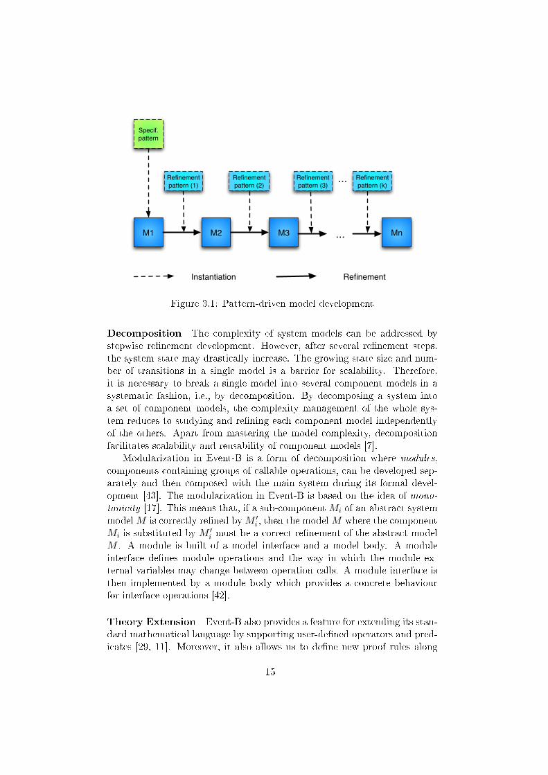
Pattern-driven formal development This approach aims to identifygeneral model transformation solutions called re�nement patterns and thenrepeatedly apply them to facilitate the re�nement process. Re�nement pat-terns are used in pattern-driven formal development to provide a basis forautomation and reusability. Pattern-driven formal development can be rep-resented as shown in Fig. 3.1. The initial model M1, the starting pointof the development, is created by instantiating a special template, calledspeci�cation pattern; this is a parametrised speci�cation. During pattern in-stantiation, the model parameters are substituted with concrete data struc-tures, while the model variables and events can be renamed. The modelconstraints given for these parameters become the theorems to be proved inorder to show that this pattern is applicable for the given concrete values.If the instantiation succeeds, the model invariant properties (together withtheir proofs) are obtained for free, i.e., without any proofs.
14
M1 M2 M3 Mn
Specif. pattern
Refinement pattern (1)
...
Refinement pattern (2)
Refinement pattern (3)
Refinement pattern (k)
...
Instantiation Refinement
Figure 3.1: Pattern-driven model development
Decomposition The complexity of system models can be addressed bystepwise re�nement development. However, after several re�nement steps,the system state may drastically increase. The growing state size and num-ber of transitions in a single model is a barrier for scalability. Therefore,it is necessary to break a single model into several component models in asystematic fashion, i.e., by decomposition. By decomposing a system intoa set of component models, the complexity management of the whole sys-tem reduces to studying and re�ning each component model independentlyof the others. Apart from mastering the model complexity, decompositionfacilitates scalability and reusability of component models [7].
Modularization in Event-B is a form of decomposition where modules,components containing groups of callable operations, can be developed sep-arately and then composed with the main system during its formal devel-opment [43]. The modularization in Event-B is based on the idea of mono-tonicity [17]. This means that, if a sub-component Mi of an abstract systemmodelM is correctly re�ned byM ′i , then the modelM where the componentMi is substituted by M ′i must be a correct re�nement of the abstract modelM . A module is built of a model interface and a model body. A moduleinterface de�nes module operations and the way in which the module ex-ternal variables may change between operation calls. A module interface isthen implemented by a module body which provides a concrete behaviourfor interface operations [42].
Theory Extension Event-B also provides a feature for extending its stan-dard mathematical language by supporting user-de�ned operators and pred-icates [29, 11]. Moreover, it also allows us to de�ne new proof rules along
15

with these notations. Both additional notations and proof rules are de�nedas a theory component that can be then used in future Event-B models. Atheory can consist in new algebraic types, new operators and new proof rulesand their validation is ensured by proving the generated proof obligations.The theory feature enables the de�nition of reusable types, operators as wellas proof rules as a library of theories that can be employed in Event-B modelsand development processes.
3.2 Statistical Model Checking in Uppaal
Numerical model checking accurately computes the probability that a systemsatis�es a temporal logic property. However, the applicability of numericalmodel checking is generally limited to systems with a small number of states.The state-number restriction in model checking does not allow to verify largemodels such as protocols in large networks or under di�erent conditions.Therefore, for the veri�cation of quantitative properties of network protocols,we need to employ other methods, such as statistical model checking (SMC).SMC [73, 61] combines ideas of model checking and simulation with the aimof supporting quantitative analysis as well as addressing the size barrier thatprevents useful analysis of large models.
Statistical model checking addresses the veri�cation problem of large sys-tems by providing a statistical evidence for the satisfaction or violation ofthe speci�cation [73, 61]. It computes the probability that a system modelsatis�es a system property. For instance, in protocol veri�cation, it can com-pute the probability of route discovery in the presence of mobile nodes in thenetwork. This problem cannot be solved by numerical model checking tech-niques due to the state explosion problem. Thus, the idea of this approachis to conduct some simulation of the system and to verify if this simulationsatis�es a given property.
SMC is based on a formal semantic of systems and uses Monte Carlo sam-pling and hypothesis testing to reason on behavioural properties of systems.In fact, a system is simulated for many runs. The number of simulation runsneeded in SMC-Uppaal is computed by using Cherno�-Hoe�ding bounds,that are independent of the size of the system. Extracted samples are mon-itored by testing techniques and a statistical evidence for the correctness ofthe system with respect to the system properties is provided. The statisticalevidence is an accurate estimation, because it is computed on sample runs ofthe system according the distribution de�ned by the system. Therefore theprobability measures follow the same distribution as de�ned by the system.
SMC-Uppaal supports the analysis of price timed-automata (PTAs). PT-As are timed-automata in which clocks may have di�erent rates in di�er-ent locations. PTAs are input-enabled, deterministic automata that com-
16

municate via broadcast channels and shared variables to build networks ofprice timed-automata (NPTA). Properties of NPTAs are expressed in cost-constraint temporal logic [31, 64] over runs of the form ψ = ♦x≤c ϕ, where ϕis a state-predicate, x is an observer clock which never resets and c ∈ R≥0 isa bound. Each run is encoded as a Bernouli random variable that is true ifthe run satis�es ϕ with x ≤ c and false otherwise. For an NPTA M , PM (ψ)is the probability that a random run of M satis�es ϕ.
To answer the problem of checking PM (ψ) ≥ p (p ∈ [0, 1]), statisticalmodel checking algorithms are used. We can have two types of analysis:qualitative and quantitative. In qualitative analysis, the goal is to answer ifthe probability PM (♦x≤c ϕ) related to a given NPTA M is greater or equalthan a certain threshold θ:
PM (♦x≤c ϕ) ≥ θ
In quantitative analysis, the goal is to �nd the probability that a random runof a given NPTAM satis�es ♦x≤c ϕ. The qualitative analysis issue in SMC-Uppaal is addressed by the hypothesis testing approach. In this approach,the hypothesis H : p = PM (♦x≤c ϕ) ≥ θ is tested against K : p < θ. Thequantitative analysis issue in SMC-Uppaal is addressed by the Monte Carloapproach. Namely, the number of runs needed to produce an approximationinterval [p− ε, p+ ε], where p denotes the probability of ψ with a con�dence1 − α is computed. Here, α stands for the probability of false negativesand ε stands for the probabilistic uncertainty. These parameters are used tospecify the statistical con�dence on the result.
17

18

4. Reusable Formal Network Archi-
tectures
In this section we put forward the contribution of the original publicationsthat make up this dissertation. In particular, we discuss the approach takenin each paper to address the reuse and correctness of networking architec-tures. Moreover, we emphasize the quantitative and quantitative analysisaspects put forward by each paper.
4.1 Reusable and correct-by-construction WSANs
In this paper, we model and analyse the functioning of a dynamic networkin Event-B. Based on this, we then derive design patterns for developingreliable dynamic networks. With respect to the three components of a net-working architecture (i.e., topology, resource management and routing), inthis paper we address the following. The network topology changes due tounpredictable failures of nodes. The resource management feature is studiedby considering two types of nodes with their corresponding homogeneousand heterogeneous connections. Routing is addressed by modelling the con-nectivity aspects of a dynamic network upon the failure of a node. A formalarchitecture for developing dynamic networks is thus proposed, includingthree main features: unpredictable topology, heterogeneous nodes and con-nectivity. These features are developed in several re�nement steps. Thestepwise methodology reduces the proofs of the system correctness at eachlevel, because in each re�nement step one feature is detailed. Dealing withone feature at each step also provides for a compositional approach. Thedeveloped dynamic network is analysed against its desirable mathematicalproperties. The main property we verify is the satis�ability of reestablish-ing connectivity in a dynamic network; this is a rather thorough example ofqualitative analysis. We put forward the reusability of our methodology viaformal design patterns. We present an abstract model of our architecturetogether with possible re�nement patterns that can be reused to develop andanalyse a particular dynamic network. Our example of a dynamic networkis a wireless sensor-actor network (WSAN).
19

4.2 Towards a reusable implementation of WSANs
In this paper we start from the same model of a networking architecture asin Paper I. Namely, we study a dynamic network whose topology changesdue to unpredictable failures and whose resource management is addressedagain via two types of nodes. However, in Paper II we take a di�erent viewon the development and reusability feature of our network. In particular, wediscuss the derivation of a dynamic network implementation from part of theabstract speci�cation presented in Paper I. In the proposed architecture ofPaper I, the network features are compacted in an individual system model:this makes it challenging to derive an implementation of a dynamic networkfrom the speci�cation. To tackle this and provide a more e�cient develop-ment approach, we employ the decomposition technique in Event-B. Moreprecisely, we develop a model for a network infrastructure and a model forthe distributed nodes, using the modularization technique in Event-B. Wede�ne node modules which have their own state and invariant properties.The correctness of the decomposed model follows from the proof obligationsthat express the consistency between the abstract and the re�ned model;again, we put forward a qualitative analysis for our proposed architecture.By decomposing the model of a dynamic network, we provide means to reusethe node modules and the network infrastructure to develop speci�c dynamicnetwork architectures, which can then be e�ciently implemented.
4.3 A reusable mobility model for analysing ad-hoc
networks
In this paper, we focus on modelling a dynamic network, whose topologyevolves due to node mobility. The resource management and the routingfeatures are considered as general as possible, and hence, have no explicitde�nition in this paper. Our aim here is to e�ciently model node mobility, inorder to evaluate the performance of network protocols by simulations. Wepropose an abstract, reusable, automata-based model that de�nes mobilityas probabilistic changes in the topology. The model is instantiated to twospeci�c mobility models, namely random walk and random waypoint, toexpress reusability of the automata-based model. The proposed mobilitymodel provides a sound foundation for reasoning about the behaviour ofdynamic networks such as mobile ad-hoc networks. In other words, the modelis intended to be used in conjunction with protocols for e�cient performanceanalysis of dynamic network protocols and thus provides the basis for aquantitative analysis of the proposed architecture.
20

4.4 Quantitative analysis of routing in ad-hoc net-
works
In this paper, we focus on the quantitative analysis of the dynamic networkmodel proposed in Paper III. We analyse several variants of the AODV rout-ing protocol and compare them, to determine optimal versions. We model adynamic network where the topology changes are due to node mobility. Theresource management feature is addressed by considering two types of nodesin the network: static and mobile. The routing feature is studied by mod-elling the AODV routing protocol and its variants. We develop a mobilitymodel as a price timed-automata. AODV and its variants are speci�ed usingalso priced timed-automata. The probability of route discovery is analysed inall AODV variants to determine which variant performs better with respectto route discovery. The mobility model is an independent time automatathat can be reused for analysis of network protocols in networks where thetopology changes due to mobility. The mobility model is a parametrized tem-plate which can be instantiated to provide di�erent patterns for the changingtopology.
4.5 Reusable and correct-by-construction NoC ar-
chitectures
In this paper, we propose a formal architecture for the e�cient developmentof static networks. In particular, we develop a network-on-chip architectureusing Event-B. We address the modelling of a static topology and focus onthe 3D mesh topology. The resource management feature is modelled byconsidering network resources such as packets, channels and bu�ers. Byconsidering the packet as a resource, we focus our development on packet-based switching mechanisms. The routing feature is addressed by studyingunicast communication. These network features are developed in three re-�nement steps. The initial abstract model includes a static topology that isindependent of the real physical layout, a set of messages and the unicastcommunication functionality. In the �rst re�nement steps the mesh topol-ogy and the concept of channels are added and in the second re�nement stepthe concept of bu�er is added. Already in the �rst abstract model, the su�-cient condition for constructing a correct network architecture is de�ned andproved. The su�cient condition is that all injected messages are received bytheir destinations. In the next re�nement steps the condition is developed totake into account the speci�c features of these steps. In each re�nement step,the proving process guides us to develop a correct architecture. The re�ne-ment decisions are taken so that each of the three models can be reused todevelop and analyse speci�c network designs at di�erent abstraction levels.
21

We demonstrate the reuse of our development, by modelling and analysinga particular routing algorithm, as a re�nement of our third model. Thusin this paper we put forward a qualitative analysis of the proposed networkarchitecture.
4.6 Reusable and correct-by-construction multicast
routing in NoC architectures
In this paper, we propose a reusable architecture for static networks witha multicast communication scheme. We start from the same topology andresource management models of a networking architecture as in Paper V;however, multicast communication is taken into account for modelling therouting feature. The network development is performed in three re�nementsteps. In the initial model, structural components and su�cient conditionsfor modelling and analysing multicast communication are proposed. In thenext two re�nement steps, the structures are re�ned to add the concept ofchannel and bu�er. The su�cient condition is that all injected messages arereceived by all their destinations; this condition is preserved by our devel-opment. The generic models specify the primitive structures and su�cientconditions for constructing a correct network, regardless of any speci�c net-work architecture. The generic aspect of the proposed development is keyfor reusability and provides another example of qualitative analysis of staticnetwork architectures.
4.7 A correct-by-construction framework for devel-
oping static network architectures
In this paper, we propose a hierarchical framework for the development ofcorrect static network systems. We combine models of static networks pro-posed in Paper V and Paper VI for developing network-on-chip systems, togain a more general model that can be reused for a wider class of static net-works. The framework addresses the modelling of a static network regardlessof its physical layout. To study the resource management feature, we con-sider packets, �its, channels and bu�ers. By considering both packets and�its, our framework becomes suitable for modelling both packet-based and�it-based switching mechanisms. The routing feature is addressed by consid-ering both unicast and multicast communication. The framework providesa clear separation between architectural and algorithmic aspects of networkdevelopment and, as a consequence, provides means for easier discoveringerror resources in the development cycle. The framework is constructed inEvent-B and is an abstract and parametric description of static networks;
22
its correctness is satis�ed by proving the satisfaction of su�cient conditions.The strength of our framework consists in reusability. The pre-proved frame-work provides a reusable network infrastructure that allows designers to de-velop speci�c network architectures correctly by proving all proof obligationsin their development. It also provides the means to construct a library ofveri�ed components to be employed for the development and qualitativeanalysis of a speci�c network design.
4.8 A reusable and correct-by-construction network
theory
In this paper we strengthen the framework proposed in Paper VII by amend-ing a set of basic formal theories for developing network architectures at anabstract level. The purpose of this extension is to use lessons learned fromprevious architectural developments to address our ultimate aim, i.e., pro-viding a network theory that can be reused for the development of correctnetworked systems. We address the modelling of a generic topology thatcan represent both static and dynamic topologies. The resource manage-ment feature is modelled by considering a message, as a general conceptthat can be instantiated to packets and �its; we also consider channels andbu�ers. The routing feature is addressed by studying general communicationschemes that can be seen as unicast and multicast or adaptive and deter-ministic. For these features we de�ne and prove correct rules as theories inEvent-B. As theories are general, they are reusable for the development ofcorrect networked systems. In fact, we develop a library of pre-proved rules,representing the functionality of network features in a hierarchical manner.The pre-proved rules facilitate the design and veri�cation of networked sys-tems throughout the network development cycle. The developed rules canbe reused as original constructors in Event-B that alleviate the di�culty ofusing formal methods for network development. Another advantage of usingsuch rules is that the designer can freely develop networked systems for qual-itative analysis of other features of networked systems without consideringre�nement decisions that have been taken in our previous works.
23

24

5. Related Approaches
In this chapter, we review existing literature that we �nd relevant to this dis-sertation. First, we discuss formal approaches for modelling and analysingdynamic networks. Second, we outline approaches for correctly develop-ing static networks. Third, general approaches for speci�cation and veri-�cation of network protocols without considering certain characteristics ofdynamic/static networks are discussed. Finally, we discuss correct-by con-struction approaches for system development.
5.1 Modelling and Analysing Dynamic Networks
Formal modelling and analysis of dynamic networks has been widely ad-dressed in the literature. Bernardeschi et al. [22] propose an approach basedon the PVS theorem prover [6] to analyse protocols for sensor networks indynamic scenarios with mobile nodes. They develop a formal speci�cationfor the reverse path forwarding (RPF) algorithm, which is a broadcast rout-ing method. RPF exploits the information contained in the routing table todeliver packets generated by a base station to all other nodes in a multi-hopnetwork. They use PVS to verify correctness properties of RPF. The simi-larity of their approach to ours consists in using abstraction and re�nementtechniques in network development.
Bhargavan et al. [23] use the theorem prover HOL [4] and the modelchecker SPIN [8] together to prove properties of routing protocols in ad-hocnetworks. They verify the AODV routing protocol using their method andidentify errors in the AODV speci�cation that can lead to a deadlock situa-tion. Fehnker et al. [36] propose a process algebra for wireless networks toverify properties of network protocols. They model AODV in this frameworkand derive a Uppaal model of AODV from their process algebra model tocheck desired properties of AODV against all topologies of up to 5 nodes[35]. This exhaustive search allows to quantify in how many topologies aparticular error can occur. They also analyse the AODV model in a dy-namic network when a link breaks. Continuing this line of research, Hoefnerand McIver [40] use the SMC extension of Uppaal to verify properties of theAODV in larger networks, with up to 100 nodes. We extend this series of
25

studies on the AODV routing algorithm by adding a mobility model. Wecapture a dynamic network topology and analyse properties of AODV.
Xiong et al. [72] propose a timed model to verify routing protocols forwireless ad-hoc networks, based on the idea of topology approximation. Thisapproach describes aggregate behaviour of nodes when their long term av-erage behaviours are of interest. They use Colored Petri Nets (CPN) [44]to demonstrate the applicability of their approach by modelling and verify-ing AODV. Yuan et al. [74] model the dynamic topology changes of ad-hocnetworks with Colored Petri Nets and verify a routing protocol for mobilenetworks called Destination-Sequenced Distance Vector (DSDV) [57] to ex-emplify their technique.
The purpose of the outlined studies consists in mostly specifying and ver-ifying existing network protocols. Our approach focuses on the developmentof correct network protocols by investigating the genericity and reusabilityof proof-based models. We propose su�cient architectural conditions andstructural design patterns and methods to design correct network protocolsthat satisfy the essential conditions of network architectures. Our approachwould ensure that properties established on the abstract models are satis�edby the actual implementation.
5.2 Modelling and Analysing Static Networks
The literature on modelling and analysing static networks has grown in therecent years. Schmaltz and Borrione [58] propose a general model of on-chipcommunication architectures, called GeNoC, in order to facilitate the de-sign of correct network-on-chip systems. Their model is developed using theACL2 theorem prover [1]. Three independent groups of functions, namelyrouting and topology, scheduling, and interfaces, form the foundation of themodel. Moreover, the su�cient constraints that these functions should sat-isfy are introduced in order to prove the correctness of the model. Thisseparation of functions allows for a stepwise design and veri�cation, whereat each step only one group of functions is considered. We also adopt thisfeature in our framework. The GeNoC model is used to prove propertiesof communication functions for the routing algorithm of the HERMES NoC[26, 68] and of the spidergon NoC [27]. The purpose of the above stud-ies is to verify the overall correctness of these NoC systems. Verbeek andSchmaltz [65, 66, 67] extend GeNoC to provide su�cient constraints thatensure deadlock-free routing and liveness of the design.
The genericity and reusability proposed by GeNoC are similar to ourapproach. However, we provide these features using the powerful techniqueof re�nement, to manage the complexity of the development as well as of theproofs. Moreover, we have the possibility to derive an implementation of a
26

certain NoC architecture from a developed model, using re�nement.Andriamiarina et al. [14] have only recently proposed a formalism for
NoC architectures based on incremental design and proof theory. They de-velop their speci�cation using the Event-B formalism to verify an adaptiveand fault-tolerant routing technique. They focus only on a particular typeof routing technique in their development, which reduces the generalisationof the development.
Chen et al. [30] propose a formal modelling approach to verify routingprotocols for NoC architectures. They provide a guideline for constructingformal models of NoC designs and propose a methodology for verifying NoCproperties such as deadlock freedom and tra�c congestion. For the formalveri�cation task, a model checker called State Graph Manipulators (SGM)[41] is used and they show the applicability of their approach by developingand verifying a speci�c NoC, namely the Bidirectional Channel Network-on-Chip (BiNoC) [48]. However, due to applying model checking in veri�cation,this work su�ers from the state explosion problem. Therefore, the numberof nodes is a concern in this veri�cation while the number of nodes is not alimitation for our work.
Palaniveloo et al. [55] propose a formal model of the Hermes NoC routerarchitecture and its communication scheme using their own HeterogeneousProtocol Automata (HPA) formalism. The HPA language is developed inthis work to model the behaviour of communication modules as event-basedtransition systems. They also map the automata model of NoC developedin HPA to PROMELA speci�cation language of the SPIN model checker [8]for veri�cation.
Böhm [24] proposes a formal framework for modelling and verifying on-chip communication protocols in the Isabelle/HOL theorem prover [54, 5].The proposed methodology is based on incremental modelling in which ab-stract building blocks and composition rules are initially speci�ed. Thisrelates to our work of using an incremental approach that interleaves modelconstruction and veri�cation. Some other re�nement approaches to the de-sign and veri�cation of on-chip communication architectures have also beenused in [25, 38].
5.3 Architectural Development of Networked Sys-
tems
The formal approaches discussed in Sections 5.1 and 5.2 entail the speci�ca-tion and veri�cation of networks at a high and abstract level. The high-levelspeci�cation should be transformed to an actual implementation while itensures the correctness of its properties. The correct transformation of ahigh-level speci�cation to an implementation is a challenge. To tackle this
27

challenge, there are a series of studies on the use of formal analysis tech-niques to reason about network protocol correctness throughout the networkdevelopment cycle [45, 37]. They mostly propose domain speci�c languagesin order to develop correct network protocols.
Karsten [45] axiomatically speci�es basic inter-networking concepts. Thisis then employed to construct a theoretically sound framework, to express ar-chitectural invariants and the deliverability of messages even in the presenceof network dynamism. A meta-language is proposed for the rapid imple-mentation of di�erent packet forwarding schemes. The concepts and themeta-language derived from them aim at clarifying the essential architectureof the Internet. Moreover, they provide a bridge between formal proofs onnode reachability using a particular forwarding scheme and an implemen-tation of that scheme. The purpose of this approach is to provide for ane�cient development of networked systems, by accelerating the constructionof their essential aspects.
To address e�ciency in the modelling and analysis of network architec-tures, Khoury et al. [46] present a design methodology based on the Alloylanguage, which is based on relations and �rst-order predicate logic. Theconcept of architectural style is at the core of this formalism in order tode�ne a precise, common design vocabulary for a class of architectures. Themethodology is demonstrated by describing a model of a class of network ar-chitectures called FARA [3]. FARA is an abstract high-level network modelin which the Internet architecture is modelled, to enable decoupling of end-point names from network addressing.
Another approach that deals with e�cient network development is pro-posed by Gri�n and Sobrinho [37]. They use a high-level and declarativelanguage to model routing and its correctness properties by proposing anapproach called Metarouting. The theoretical basis of Metarouting is theRouting Algebra framework of Sobrinho [62]. These formal models use acorrect-by-construction approach in which the veri�cation of convergence isaccomplished once for the idealized algebra, and any routing protocol thatimplements the algebra is correct.
Wang et al. [69, 70] propose a formally veri�able networking (FVN) ap-proach for unifying the design, speci�cation, implementation and veri�cationof networking protocols. The FVN framework uses a formal logical founda-tion to specify the behaviour and the properties of network protocols and ofthe abstract network meta-model. A theorem prover such as PVS [6] or Coq[2] is used to verify the speci�ed formal properties of declarative networkprotocols.
To bridge the high-level speci�cation with the implementation of net-worked systems in these related works, their authors propose new languagesfor which the theoretical bases are proved using formal methods. An impor-tant advantage of our method for network development consists in reusing an
28

existing language to bridge high-level speci�cations with implementations,namely Event-B; in our approach, we handle this bridging challenge with thepowerful re�nement technique.
5.4 Correct-by-Construction System Development
Correct-by-construction methods have been applied in several domains re-lated to networked systems such as product line analysis, train systems, etc.Lamprecht et al. [47] use the correct-by-construction approach to propose amodelling framework for the analysis of product lines. They combine synthe-sis technology with a constraint-oriented approach to guarantee the validityof system properties. The validity of a variant of a product line is satis-�ed if properties of the high-level model of the product line are preserved.They present the applicability of their approach by illustrating it on a co�eemachine example.
Moller et al. [51] verify railway systems through CSP||B modelling andanalysis. In [52], they propose a structured way of analysis for interlockingrailway systems by applying the correct-by-construction approach. Theypropose model checking of the abstract model to ensure the safety properitiesthat hold in the concrete models as well.
29

30

6. Discussion
In this �nal section, we outline the main achievements put forward in thisdissertation as well as point out future research directions.
Summary In this dissertation, we have aimed at contributing to the de-velopment of networked architectures for e�ciency and reliability, where bye�ciency we refer to the possibility of reusing such architectures and by re-liability we refer to developing correct models with respect to their speci�ca-tions. In order to provide reusable architectures, we need to construct themin certain ways; for verifying the correctness of the architectures, we need toanalyse them with respect to certain properties. Our research method con-sists in applying formal methods in order to achieve our aims, in particularthe abstraction and re�nement techniques.
The Challenge A very interesting challenge in applying formal methods inthe domain of networked systems consists in determining a formal theory ofnetwork architectures and, as a consequence, providing reusable, pre-proveddesign rules. Determining a formal theory of networked architectures re-quires generic models. These models consist of the essential components ofany networked system together with their relations. In addition, such modelsneed to preserve the global correctness of the network. Providing reusable,pre-proved design rules needs considering individual components of a net-worked system and their variations. If a correct model of a component andits variants can be developed independently of other components, then it canbe reused in the development of a certain architecture.
What we have achieved Our goal has been to develop approaches forthe formal construction and analysis of networked systems that support:
(1) A reusable and correct-by-construction development of networked sys-tems
(2) Precise and sound foundation for rigorous qualitative and quantitativeanalysis
31

To achieve this goal, we have developed three artefacts:
(A) A formal generic architectural model for the correct development ofnetworked systems
(B) Methods for reusable networked system development
(C) A library of rules for developing and analysing networked systems
Artefact (A), a formal generic architectural model for the correct de-velopment of networked systems, consists of high-level generic models forspecifying networked systems and their properties that are preserved underre�nement. General high-level models represent the conceptual frameworkof networked systems as a general architectural model of networks. The gen-eral architectural model can be instantiated to a particular architecture byre�nement, so that the functional correctness is preserved; this is an answerto the correct development of networked systems. As network developmentas we proposed it does not start from scratch, but from using the generalarchitectural model, this is also an answer to the reusable development ofnetworked systems. Artefact (A) is therefore an answer to goal (1).
Artefact (B), consisting of the methods for reusable networked systemdevelopment, de�nes processes in which models can be speci�ed and shown tobe reusable. The methods that are used to support reusability in this thesisare: abstraction, re�nement, re�nement patterns, modularisation, theoryextension and automata-based templates. Artefact (B) is therefore an answerto goal (1), as well.
Artefact (C), consisting of a library of rules for developing and analysingnetworked systems, consists of a set of fundamental design rules which de�nethe individual architectural components of networked systems that can beseparately reused in the development and analysis of certain architectures.Artefact (C) is therefore an answer to goal (1) and (2).
Future Directions We can put forward several possible directions for fu-ture work. We have proposed a network framework consisting of high-leveldescriptions of networked systems, together with their functional properties.An interesting research direction consists in further extending of the currentframework by including other features of networked systems. Such an exten-sion could support, for instance, the analysis of real-time and non-functionalproperties such as power consumption, delay and performance during devel-opment. Moreover, the applicability of the framework could be examined byusing it in the development and analysis of various networks. One could in-vestigate how �exible the framework is to analyse a wider class of networkedsystems and to support di�erent views of development in our framework.
32

These investigations would suggest the possible lines of the framework ex-tension. In fact, by applying the framework for the development and analysisof di�erent networked systems, two points could be highlighted: the ful�l-ment of the reusability feature and the clear modi�cations and extensionswhich could improve the framework usefulness.
Another research direction consists in extending the library of designrules, by adding new pre-proved network structures and techniques or re�n-ing the existing rules. Extending the library of pre-proved rules promotesthe e�ciency of developing reliable networked systems.
A signi�cant challenge in our methodology for networked systems is thatthe qualitative and quantitative analysis are not integrated. This means thatmuch e�ort is needed to model a network in such a way that either qualitativeor quantitative analysis can be performed. As a solution to this, we plan tostudy how both qualitative and quantitative analysis of networked systemscan be uni�ed at the architectural level. Ideally, we should be able to de�netransformation rules that automatically transform a developed model usedfor qualitative analysis into a model for quantitative analysis and vice versa.Even more, the automatic transformation is conceivable at the architecturallevel, where the design detail are excluded. Providing an integrated toolsupport for developing and analysing both qualitatively and quantitativelythe network architectures is also very instrumental.
33

34
7. Bibliography
[1] ACL2, online at http://www.cs.utexas.edu/ moore/acl2/.
[2] The coq proof assistanct, online at http://coq.inria.fr/, accessed20.07.2013.
[3] FARA, online at http://www.isi.edu/newarch/fara.html.
[4] HOL, online at http://www.cl.cam.ac.uk/research/hvg/hol.
[5] isabelle, online at http://isabelle.in.tum.de/.
[6] PVS speci�cation and veri�cation system, online athttp://pvs.csl.sri.com/, accessed 20.07.2013.
[7] Rodin - rigorous open development environment for complex, deliverabled7, event-b language, online at http://rodin.cs.ncl.ac.uk.
[8] SPIN, online at http://spinroot.com/spin/whatispin.html.
[9] J.-R. Abrial. The B-book: assigning programs to meanings. CambridgeUniversity Press, New York, NY, USA, 1996.
[10] J.-R. Abrial. Modeling in Event-B: System and Software Engineering.Cambridge University Press, New York, NY, USA, 1st edition, 2010.
[11] J.-R Abrial, M. Butler, S. Hallerstede, M. Leuschel, M. Schmalz, andL. Voisin. Proposals for mathematical extensions for event-b. Technicalreport, Deploy Project, 04 2010.
[12] J.-R. Abrial, M. J. Butler, S. Hallerstede, T. S. Hoang, F. Mehta,and L. Voisin. Rodin: an open toolset for modelling and reasoning inEvent-B. STTT, 12(6):447�466, 2010. http://dx.doi.org/10.1007/
s10009-010-0145-y.
[13] R. Alur and D. L. Dill. A theory of timed automata. Theoretical Com-puter Science, 126:183�235, 1994.
35

[14] M. B. Andriamiarina, H. Daoud, M. Belarbi, D. Méry, andC. Tanougast. Formal Veri�cation of Fault Tolerant NoC-based Archi-tecture. In First International Workshop on Mathematics and ComputerScience (IWMCS2012), December 2012.
[15] R. J. R. Back. Re�nement calculus, part ii: Parallel and reactive pro-grams. In REX Workshop, pages 67�93, 1989.
[16] R. J. R. Back and R. Kurki-Suonio. Distributed cooperation with actionsystems. ACM Trans. Program. Lang. Syst., 10(4):513�554, October1988.
[17] R. J. R. Back and K. Sere. From action systems to modular systems. InSoftware - Concepts and Tools, volume 17, pages 1�25. Springer-Verlag,1994.
[18] R. J. R. Back and K. Sere. Superposition re�nement of reactive systems.Formal Aspects of Computing, 8(3):324�346, 1996.
[19] R. J. R. Back and J. von Wright. Trace re�nement of action systems.In CONCUR, pages 367�384, 1994.
[20] R. J. R. Back and J. V. Wright. Re�nement calculus - a systematicintroduction. Undergraduate texts in computer science. Springer, 1999.
[21] G. Behrmann, A. David, and K. G. Larsen. A tutorial on uppaal. InSFM, volume 3185 of Lecture Notes in Computer Science, pages 200�236. Springer, 2004.
[22] C. Bernardeschi, P. Masci, and H. Pfeifer. Analysis of wireless sensornetwork protocols in dynamic scenarios. In Proceedings of the 11th Inter-national Symposium on Stabilization, Safety, and Security of DistributedSystems, SSS '09, pages 105�119, Berlin, Heidelberg, 2009. Springer-Verlag.
[23] K. Bhargavan, D. Obradovic, Carl, and A. Gunter. Formal veri�cationof standards for distance vector routing protocols. Journal of the ACM,49:538�576, 2002.
[24] P. Böhm. A framework for incremental modelling and veri�cation of on-chip protocols. In Proceedings of the 2010 Conference on Formal Meth-ods in Computer-Aided Design, FMCAD '10, pages 159�166, Austin,TX, 2010. FMCAD Inc.
[25] P. Böhm and T. Melham. A re�nement approach to design and veri�-cation of on-chip communication protocols. In Proceedings of the 2008
36
International Conference on Formal Methods in Computer-Aided De-sign, FMCAD '08, pages 18:1�18:8, Piscataway, NJ, USA, 2008. IEEEPress.
[26] D. Borrione, A. Helmy, L. Pierre, and J. Schmaltz. A generic modelfor formally verifying noc communication architectures: A case study.In Proceedings of the First International Symposium on Networks-on-Chip, NOCS '07, pages 127�136, Washington, DC, USA, 2007. IEEEComputer Society.
[27] D. Borrione, A. Helmy, L. Pierre, and J. Schmaltz. A formal approachto the veri�cation of networks on chip. EURASIP J. Embedded Syst.,2009:2:1�2:14, January 2009.
[28] P. Bulychev, A. David, K. G. Larsen, M. Mikucionis, P. Bogsted,A. Legay, and Z. Wang. Uppaal-smc: Statistical model checking forpriced timed automata. In Herbert Wiklicky and Mieke Massink, ed-itors, Proceedings 10th Workshop on Quantitative Aspects of Program-ming Languages and Systems, Tallinn, Estonia, 31 March and 1 April2012, volume 85 of Electronic Proceedings in Theoretical Computer Sci-ence, pages 1�16. Open Publishing Association, 2012.
[29] M. Butler and I. Maamria. Mathematical extension in event-b throughthe rodin theory component. Technical report, Deploy Project, 10 2010.
[30] Y.-R. Chen, W.-T. Su, P.-A. Hsiung, Y.-C. Lan, Y.-H. Hu, and S.-J. Chen. Formal modeling and veri�cation for network-on-chip. InGreen Circuits and Systems (ICGCS), 2010 International Conferenceon, pages 299�304, June.
[31] A. David, K. G. Larsen, A. Legay, M. Mikucionis, and Z. Wang. Timefor statistical model checking of real-time systems. In CAV, pages 349�355, 2011.
[32] J. W. de Bakker, W. P. de Roever, and G. Rozenberg, editors. StepwiseRe�nement of Distributed Systems, Models, Formalisms, Correctness,REX Workshop, Mook, The Netherlands, May 29 - June 2, 1989, Pro-ceedings, volume 430 of Lecture Notes in Computer Science. Springer,1990.
[33] E. W. Dijkstra. A constructive approach to the problem of programcorrectness. BIT Numerical Mathematics, 8(3):174�186, 1968.
[34] E. W. Dijkstra. A Discipline of Programming. Prentice Hall PTR,Upper Saddle River, NJ, USA, 1st edition, 1997.
37
[35] A. Fehnker, R.J. van Glabbeek, P. Höfner, A. McIver, M. Portmann,and W.L. Tan. Automated analysis of aodv using uppaal. In Proceed-ings of the 18th international conference on Tools and Algorithms forthe Construction and Analysis of Systems, TACAS'12, pages 173�187,Berlin, Heidelberg, 2012. Springer-Verlag.
[36] A. Fehnker, R.J. van Glabbeek, P. Höfner, A. McIver, M. Portmann,and W.L. Tan. A process algebra for wireless mesh networks. In H. Seidl,editor, European Symposium on Programming (ESOP'12), volume 7211of Lecture Notes in Computer Science, pages 295�315. Springer, 2012.
[37] T. G. Gri�n and J. L. Sobrinho. Metarouting. In Proceedings of the 2005conference on Applications, technologies, architectures, and protocols forcomputer communications, SIGCOMM '05, pages 1�12, New York, NY,USA, 2005. ACM.
[38] R. Ameur-Boulifa H. Mokrani. A re�nement approach to design andveri�cation of on-chip communication protocols. In Proceedings of theSAFA workshop, 2011.
[39] C. A. R. Hoare. Communicating sequential processes. Commun. ACM,21(8):666�677, August 1978.
[40] P. Höfner and A. McIver. Statistical model checking of wireless meshrouting protocols. In NASA Formal Methods Symposium (NFM'13), vol-ume unde�ned of Lecture Notes in Computer Science, page unde�ned.Springer, 2013.
[41] P.-A. Hsiung and F. Wang. A state graph manipulator tool for real-timesystem speci�cation and veri�cation. In Real-Time Computing Systemsand Applications, 1998. Proceedings. Fifth International Conference on,pages 181�188, Oct.
[42] A. Iliasov, L. Laibinis, E. Troubitsyna, and A. Romanovsky. Formalderivation of a distributed program in event b. In Proceedings of the 13thinternational conference on Formal methods and software engineering,ICFEM'11, pages 420�436, Berlin, Heidelberg, 2011. Springer-Verlag.
[43] A. Iliasov, E. Troubitsyna, L. Laibinis, A. Romanovsky, K. Varpaaniemi,D. Ilic, and T. Latvala. Supporting reuse in event b development: mod-ularisation approach. In Proceedings of the Second international con-ference on Abstract State Machines, Alloy, B and Z, ABZ'10, pages174�188, Berlin, Heidelberg, 2010. Springer-Verlag.
[44] K. Jensen. Coloured Petri Nets: Basic Concepts, Analysis Methods andPractical Use. Volume 1. Springer Publishing Company, Incorporated,2010.
38
[45] M. Karsten, S. Keshav, S. Prasad, and M. Beg. An axiomatic basis forcommunication. In Proceedings of the 2007 conference on Applications,technologies, architectures, and protocols for computer communications,SIGCOMM '07, pages 217�228, New York, NY, USA, 2007. ACM.
[46] J. Khoury, C. Abdallah, and G. Heileman. Towards formalizing net-work architectural descriptions. In Marc Frappier, Uwe Glässer, SarfrazKhurshid, Régine Laleau, and Steve Reeves, editors, Abstract State Ma-chines, Alloy, B and Z, volume 5977 of Lecture Notes in ComputerScience, pages 132�145. Springer Berlin Heidelberg, 2010.
[47] A.-L. Lamprecht, T. Margaria, I. Schaefer, and B. Ste�en. Synthesis-based variability control: Correctness by construction. In FMCO, pages69�88, 2011.
[48] Y.-C Lan, S.-H. Lo, Y.-C. Lin, Y.-H. Hu, and S.-J. Chen. Binoc: Abidirectional noc architecture with dynamic self-recon�gurable channel.In Proceedings of the 2009 3rd ACM/IEEE International Symposium onNetworks-on-Chip, NOCS '09, pages 266�275, Washington, DC, USA,2009. IEEE Computer Society.
[49] R. Milner. A Calculus of Communicating Systems. Springer-Verlag NewYork, Inc., Secaucus, NJ, USA, 1982.
[50] R. Milner. Communicating and mobile systems: the &pgr;-calculus.Cambridge University Press, New York, NY, USA, 1999.
[51] F. Moller, H. N. Nguyen, M. Roggenbach, S. Schneider, and H. Tre-harne. Csp||b modelling for railway veri�cation: The double junctioncase study. In AVOCS'12, 2012.
[52] F. Moller, H. N. Nguyen, M. Roggenbach, S. Schneider, and H. Tre-harne. De�ning and model checking abstractions of complex railwaymodels using csp||b. In HVC'2012, 2012.
[53] A. Müller. Vdm � the vienna development method, 2009.
[54] T. Nipkow, L. C. Paulson, and M. Wenzel. Isabelle/HOL � A ProofAssistant for Higher-Order Logic, volume 2283 of LNCS. Springer, 2002.
[55] V.A. Palaniveloo and A. Sowmya. Application of formal methods forsystem-level veri�cation of network on chip. In VLSI (ISVLSI), 2011IEEE Computer Society Annual Symposium on, pages 162�169, July.
[56] C. E. Perkins, E. M. Belding-Royer, and I. D. Chakeres. Ad hocon-demand distance vector (AODV) routing. Internet Draft, 2003.At http://tools.ietf.org/id/draft-perkins-manet-aodvbis-00.
txt.
39

[57] C. E. Perkins and P. Bhagwat. Highly dynamic destination-sequenceddistance-vector routing (dsdv) for mobile computers. In Proceedings ofthe conference on Communications architectures, protocols and appli-cations, SIGCOMM '94, pages 234�244, New York, NY, USA, 1994.ACM.
[58] J. Schmaltz and D. Borrione. A generic network on chip model. InProceedings of the 18th international conference on Theorem Proving inHigher Order Logics, TPHOLs'05, pages 310�325, Berlin, Heidelberg,2005. Springer-Verlag.
[59] S. Schneider and H. Treharne. Csp theorems for communicating b ma-chines. Formal Aspects of Computing, 17(4):390�422, December 2005.
[60] S. Schneider, H. Treharne, and H. Wehrheim. A csp approach to con-trol in event-b. In Proceedings of the 8th international conference onIntegrated formal methods, IFM'10, pages 260�274, Berlin, Heidelberg,2010. Springer-Verlag.
[61] K. Sen, M. Viswanathan, and G. A. Agha. Vesta: A statistical model-checker and analyzer for probabilistic systems. In Quantitative Evalu-aiton of Systems (QEST'05), pages 251�252. IEEE, 2005.
[62] J. L. Sobrinho. Network routing with path vector protocols: theory andapplications. In Proceedings of the 2003 conference on Applications,technologies, architectures, and protocols for computer communications,SIGCOMM '03, pages 49�60, New York, NY, USA, 2003. ACM.
[63] J. M. Spivey. The Z notation: a reference manual. Prentice-Hall, Inc.,Upper Saddle River, NJ, USA, 1989.
[64] T. Teige, A. Eggers, and M. Fränzle. Constraint-based analysis of con-current probabilistic hybrid systems: An application to networked au-tomation systems. Nonlinear Analysis: Hybrid Systems, 5(2):343�366,2011.
[65] F. Verbeek and J. Schmaltz. Formal speci�cation of networks-on-chips:deadlock and evacuation. In Design, Automation Test in Europe Con-ference Exhibition (DATE), 2010, pages 1701 �1706, march 2010.
[66] F. Verbeek and J. Schmaltz. Automatic veri�cation for deadlockin networks-on-chips with adaptive routing and wormhole switching.In Proceedings of the Fifth ACM/IEEE International Symposium onNetworks-on-Chip, NOCS '11, pages 25�32, New York, NY, USA, 2011.ACM.
40

[67] F. Verbeek and J. Schmaltz. On necessary and su�cient conditionsfor deadlock-free routing in wormhole networks. IEEE Transactions onParallel and Distributed Systems, 22(12):2022�2032, 2011.
[68] F. Verbeek and J. Schmaltz. Easy formal speci�cation and validation ofunbounded networks-on-chips architectures. ACM Trans. Des. Autom.Electron. Syst., 17(1):1:1�1:28, January 2012.
[69] A. Wang, P. Basu, B. T. Loo, and O. Sokolsky. Declarative networkveri�cation. In Proceedings of the 11th International Symposium onPractical Aspects of Declarative Languages, PADL '09, pages 61�75,Berlin, Heidelberg, 2009. Springer-Verlag.
[70] A. Wang, L. Jia, C. Liu, B. T. Loo, O. Sokolsky, and P. Basu. Formallyveri�able networking. In Lakshminarayanan Subramanian, Will E. Le-land, and Ratul Mahajan, editors, HotNets. ACM SIGCOMM, 2009.
[71] N. Wirth. Program development by stepwise re�nement. Communica-tions of the ACM, 14(4):221�227, 1971.
[72] C. Xiong, T. Murata, and J. Tsai. Modeling and simulation of rout-ing protocol for mobile ad hoc networks using colored petri nets. InProceedings of the conference on Application and theory of petri nets:formal methods in software engineering and defence systems - Volume12, CRPIT '02, pages 145�153, Darlinghurst, Australia, Australia, 2002.Australian Computer Society, Inc.
[73] H. Younes. Veri�cation and Planning for Stochastic Processes withAsynchronous Events. PhD thesis, Carnegie Mellon University, 2004.
[74] C. Yuan, J. Billington, and J. Freiheit. An abstract model of routing inmobile ad hoc networks. In Sixth Workshop and Tutorial on PracticalUse of Coloured Petri Nets and the CPN Tools, pages 137�156, Aarhus,Denmark, October 2005. DAIMI.
41

42

Complete List of Publications
1. Peter Höfner, and Maryam Kamali. Quantitative Analysis of AODVand its Variants on Dynamic Topologies using Statistical Model Check-ing, In V. Braberman and L. Fribourg (Eds.) Proceedings of the 11thInternational Conference on Formal Modeling and Analysis of TimedSystems - FORMATS 13, Lecture Notes in Computer Science Vol.8053, pp. 121-136, Springer-Verlag, 2013.
2. Ansgar Fehnker, Peter Höfner, Maryam Kamali, and Vinay Mehta.Topology-based Mobility Model for Wireless Networks, In K. Joshiet al. (Eds.) Proceedings of the 10th International Conference onQuantitative Evaluation of Systems conference - QEST 13, LectureNotes in Computer Science Vol. 8054, pp. 389-404, Springer-Verlag,2013.
3. Maryam Kamali, Mats Neovius, Luigia Petre and Petter Sandvik.Formal Development of System of Systems, Accepted to ISRN Soft-ware Engineering Journal, Hindawi Publishing Corporation, 2013. (Inpress)
4. Maryam Kamali, Linas Laibinis, Luigia Petre, and Kaisa Sere. A Dis-tributed Implementation of a Network Recovery Algorithm, In Inter-national Journal of Critical Computer-Based Systems (IJCCBS), Vol.4, No. 1, pp. 45-68. Inderscience Publishers, 2013.
5. Maryam Kamali, Luigia Petre, and Kaisa Sere. NetCorre: A Hierarchi-cal Framework and Theory for Network Design (Submitted to Scienceof Computer Programming Journal), April, 2013.
6. Maryam Kamali, Linas Laibinis, Luigia Petre, and Kaisa Sere. FormalDevelopment of Wireless Sensor-Actor Networks, In Science of Com-puter Programming (SCP) Journal. Elsevier, 2012. DOI: 10.1016/j.scico.2012.03.002.
7. Maryam Kamali, Luigia Petre, Kaisa Sere, and Masoud Daneshtalab.Re�nement-Based Modeling of 3D NoCs, In F. Arbab and M. Sir-jani (Eds.) Proceedings of the 4th IPM International Conference on
43

Fundamentals of Software Engineering - FSEN 11, Lecture Notes inComputer Science Vol. 7141, pp. 236-252, Springer-Verlag, 2012.
8. Masoud Daneshtalab, Maryam Kamali, Masoumeh Ebrahimi, SaeedMohammadi, Ali Afzali-Kusha, Juha Plosila. Adaptive Input-OutputSelection Based On-Chip Router Architecture, In Journal of LowPower Electronics, Volume 8, Number 1, pp. 11-29, February 2012.
9. Maryam Kamali, Luigia Petre, Kaisa Sere, and Masoud Daneshta-lab. CorreComm: A Formal Hierarchical Framework for Communi-cation Designs, In Proceedings of the 2nd IEEE International Confer-ence on Networked Embedded Systems for Enterprise Applications -NESEA2011, pp. 1-7. IEEE Computer Society, December, 2011.
10. Maryam Kamali, Luigia Petre, Kaisa Sere, and Masoud Daneshtalab.Formal Modeling of Multicast Communication in 3D NoCs. In P. Kit-sos and S. Niar (Eds.) Proceedings of the 14th Euromicro Conferenceon Digital System Design - DSD 2011, pp. 634-642. IEEE/Euromicro,August 2011.
11. Maryam Kamali, Luigia Petre, Kaisa Sere, Masoud Daneshtalab. AFormalization of 3D NoCs, In M. Waldén, and L. Petre (Eds.) Proceed-ings of the 22nd Nordic Workshop on Programming Theory - NWPT2010,TUCS Technical Reports, No. 57, pp. 79-81, November 2010.
12. Maryam Kamali, Linas Laibinis, Luigia Petre and Kaisa Sere. Self-Recovering Sensor-Actor Networks, In M. Mousavi and G. Salaün (Eds.)Proceedings of the 9th International Conference on the Foundations ofCoordination Languages and Software Architectures - FOCLASA2010,pp. 47-61. EPTCS, September, 2010.
13. Maryam Kamali, Linas Laibinis, Luigia Petre and Kaisa Sere. Recon-structing Coordination Links in Sensor-Actor Networks, In C. Jensen(Eds.) Proceedings of the 4th Nordic Workshop on Dependability andSecurity - NODES 2010, pp. 1-10, June 2010.
14. Mohsen Shari�, Saeed Sedighian and Maryam Kamali. RechargingSensor Nodes Using Implicit Actor Coordination in Wireless SensorActor Networks, In Scienti�c Research Journal of Wireless Sensor Net-work, Vol 2, N. 2, pp. 123-131, February 2010.
15. Maryam Kamali, Mohsen Shari� and Saeed Sedighian. A DistributedRecovery Mechanism for Actor-Actor Connectivity in Wireless SensorActor Networks, In Proceedings of the 4nd IEEE International Con-ference on Intelligent Sensors, Sensor Networks and Information Pro-cessing - ISSNIP 2008, pp. 183-188, December 2008.
44

Part II
Original Publications
45

Paper I
Formal Development of Wireless Sensor-Actor
Networks
Maryam Kamali, Linas Laibinis, Luigia Petre and Kaisa Sere
Originally published in: Science of Computer Programming (SCP) Journal,Elsevier, 2012. In press, DOI: 10.1016/j.scico.2012.03.002.
Based on the publication: Maryam Kamali, Linas Laibinis, Luigia Petre andKaisa Sere. Self-Recovering Sensor-Actor Networks, In Proceedings of the 9thInternational Conference on the Foundations of Coordination Languages andSoftware Architectures - FOCLASA2010, pp. 47-61. EPTCS, September,2010.
47

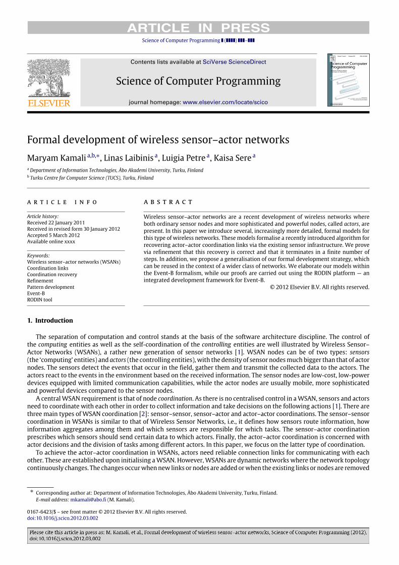
Science of Computer Programming ( ) –
Contents lists available at SciVerse ScienceDirect
Science of Computer Programming
journal homepage: www.elsevier.com/locate/scico
Formal development of wireless sensor–actor networksMaryam Kamali a,b,∗, Linas Laibinis a, Luigia Petre a, Kaisa Sere a
a Department of Information Technologies, Åbo Akademi University, Turku, Finlandb Turku Centre for Computer Science (TUCS), Turku, Finland
a r t i c l e i n f o
Article history:Received 22 January 2011Received in revised form 30 January 2012Accepted 5 March 2012Available online xxxx
Keywords:Wireless sensor–actor networks (WSANs)Coordination linksCoordination recoveryRefinementPattern developmentEvent-BRODIN tool
a b s t r a c t
Wireless sensor–actor networks are a recent development of wireless networks whereboth ordinary sensor nodes and more sophisticated and powerful nodes, called actors, arepresent. In this paper we introduce several, increasingly more detailed, formal models forthis type of wireless networks. These models formalise a recently introduced algorithm forrecovering actor–actor coordination links via the existing sensor infrastructure. We provevia refinement that this recovery is correct and that it terminates in a finite number ofsteps. In addition, we propose a generalisation of our formal development strategy, whichcan be reused in the context of a wider class of networks. We elaborate our models withinthe Event-B formalism, while our proofs are carried out using the RODIN platform — anintegrated development framework for Event-B.
© 2012 Elsevier B.V. All rights reserved.
1. Introduction
The separation of computation and control stands at the basis of the software architecture discipline. The control ofthe computing entities as well as the self-coordination of the controlling entities are well illustrated by Wireless Sensor–Actor Networks (WSANs), a rather new generation of sensor networks [1]. WSAN nodes can be of two types: sensors(the ‘computing’ entities) and actors (the controlling entities),with the density of sensor nodesmuchbigger than that of actornodes. The sensors detect the events that occur in the field, gather them and transmit the collected data to the actors. Theactors react to the events in the environment based on the received information. The sensor nodes are low-cost, low-powerdevices equipped with limited communication capabilities, while the actor nodes are usually mobile, more sophisticatedand powerful devices compared to the sensor nodes.
A centralWSAN requirement is that of node coordination. As there is no centralised control in aWSAN, sensors and actorsneed to coordinate with each other in order to collect information and take decisions on the following actions [1]. There arethree main types of WSAN coordination [2]: sensor–sensor, sensor–actor and actor–actor coordinations. The sensor–sensorcoordination in WSANs is similar to that of Wireless Sensor Networks, i.e., it defines how sensors route information, howinformation aggregates among them and which sensors are responsible for which tasks. The sensor–actor coordinationprescribes which sensors should send certain data to which actors. Finally, the actor–actor coordination is concerned withactor decisions and the division of tasks among different actors. In this paper, we focus on the latter type of coordination.
To achieve the actor–actor coordination in WSANs, actors need reliable connection links for communicating with eachother. These are established upon initialising aWSAN. However,WSANs are dynamic networkswhere the network topologycontinuously changes. The changes occurwhennew links or nodes are addedorwhen the existing links or nodes are removed
∗ Corresponding author at: Department of Information Technologies, Åbo Akademi University, Turku, Finland.E-mail address:[email protected] (M. Kamali).
0167-6423/$ – see front matter© 2012 Elsevier B.V. All rights reserved.doi:10.1016/j.scico.2012.03.002

2 M. Kamali et al. / Science of Computer Programming ( ) –
Fig. 1. Three partitions created by the failed actor A1 .
due to failures, typically caused by hardware crashes or malfunctions, the lack of energy, mobility, etc. Consequently, actornodes can fail during operation of a network. As a result, a WSAN may transform into several, disconnected WSAN sub-networks, thus interrupting the actor–actor coordination. Such a separation is called a network partitioning and is illustratedin Fig. 1, where the actor nodes A1–A15 are shown to produce a network partitioning if the actor node A1 fails.
Another central WSAN requirement focuses on embedding real-time aspects. In particular, depending on an application,it might be essential to respond to sensor inputs within predefined time limits, e.g., in critical applications such as forest firedetection. Due to the real-time requirements ofWSANs, a failure of an actor node should not affect the whole actor networkfor too long. To re-establish connectivity of actor nodes, their physical movement towards each other has been proposedin [3,4]. However, during thismovement, nodes in different network partitions created by an actor failure cannot coordinate.To shorten the time of recovery, Kamali et al. [5] have proposed an algorithm for establishing new routes between non-failedactors via sensor nodes. This algorithm allows for quick reconnection of the separated partitions, beforemoving actor nodesas proposed in [3,4]. In this paper we focus on studying this recovery mechanism, which alleviates the problems caused byactor coordination failures.
There are several properties that are desirable to verify for this algorithm. First, we need to show that there is always apath via sensor nodes that can be established for the partitioned actor nodes. Second, it is important to guarantee that thenew path is the shortest one for the involved actor nodes. Assuming that the sensor network is sufficiently dense, this alsoreduces the power consumption of the sensor nodes that are employed to re-establish connection. Third, to shorten the timeof recovery as much as possible, it is desirable to re-establish connection as soon as possible. In this paper we address thefirst and the second property of the algorithm.
The contribution of our paper is threefold. First, we formalise the algorithm for self-recovering actor coordination [5]using a theorem prover tool. This allows us to better understand the functioning of the algorithm and, more importantly,to verify essential properties such as the functional correctness and termination of the recovery mechanism. An importantaspect of the recovery is that indirect links between actors are built in a distributed manner, thus ensuring self -recoveringof the network. Second, we prove that the recovery can be done at different levels, via different link types, such as director indirect actor links, in the latter case also reusing the WSAN infrastructure of sensors. This contributes to modellingfault-recovery in sensor–actor networks. Third, we explore a generalisation of the described approach to a wider class ofnetworks by using the notions of refinement patterns and pattern-driven formal development. This allows us to facilitatethe presented formal development process by identifying the development (design) steps typical for coordinating networksas well as reusing both formal models and proofs.
To model the functional correctness of the recovery algorithm, we use the mathematical concepts of tree and forest.In graph theory, a tree is a graph whose any two vertices are connected by a non-cyclic path, while a forest is a set ofdisjoint trees. As special cases, an empty graph (with no nodes) and a discrete graph on a set of vertices (with no edges) areexamples of forests. We introduce a special data structure to model a forest and use it to prove correctness properties inthe following way. When a node fails, the set of all the neighbours of the failed node is considered as a set of disconnectedtrees, i.e., a (node) forest. For instance, in Fig. 1 the nodes A2, A6, A7, A8 A9, and A12 are the neighbours of the failed nodeA1. These nodes are considered as disconnected trees, with each tree initially formed of exactly one of the nodes. Whilethe recovery process either finds or re-establishes links, these trees gradually become connected to each other. When therecovery process terminates, we show that all the trees of the forest are connected. This means that, by the end of therecovery, all the neighbours of the failed node are re-connected.
In order to prove correctness of the recoverymechanism,we employ the Event-B formalism formodellingWSANs and theproposed algorithm [5]. Event-B [6,7] is an extension of the B Method [8] for specifying distributed and reactive systems.In Event-B, a system model is gradually specified at several levels of abstraction, always ensuring that a more concretemodel is a correct development of the previous, more abstract model. The language and proof theory of Event-B are basedon predicate logic and the set theory. Correctness of stepwise construction of formal models is ensured by discharging a

M. Kamali et al. / Science of Computer Programming ( ) – 3
Machine MVariables vInvariants IEvents
Initevt1· · ·
evtN
Sees−−→
Context CCarrier Sets dConstants cAxioms A
Fig. 2. A machineM and a context C in Event-B.
set of proof obligations: if these obligations hold, then the undertaken development is mathematically shown to be correct.Event-B comes with the associated tool RODIN [7,9,10,18], which automatically discharges a part of the proof obligationsand also provides the interactive prover to discharge the remaining proofs.
The paper is organised as follows. In Section 2we discuss the Event-B formalism and also describe the recovery algorithm.In Section 3 we overview our formal development of the recovery mechanism. Sections 4–7 contain the description of ourformal models at four abstraction levels. Specifically, in Section 4 we model the direct actor link recovery mechanism.In Section 5 the abstract model is enhanced by the indirect actor link recovery. In Section 6 we introduce the sensorinfrastructure and the indirect actor link recovery via the introduced sensors. In Section 7 we model physical distancesbetween nodes to ensure the shortest indirect links via sensors. We continue in Section 8 by discussing proving aspectsregarding our formal development. In Section 9we bring forward our approach to generalisation and reuse of the introducedformal models. We survey related work in Section 10 and in Section 11 we present several concluding remarks.
2. Preliminaries
This section presents the background material for the paper. We start by overviewing the Event-B formalism. In thesecond part of the section, we describe the recovery algorithm for WSANs, which will be formalised later.
2.1. Introduction to Event-B
The B Method [8] is a formal approach for the specification and rigorous development of highly dependable software.The method has been successfully used in the development of several complex real-life applications [10,11]. Event-B [6] is aformal framework derived from the BMethod tomodel and reason about parallel, distributed and reactive systems. Event-Bhas the associated RODIN platform [7,9,10,18], which provides automated tool support for modelling and verification bytheorem proving.
Event-B Language. In Event-B, a system specification (model) is defined using the notion of a machine [10] operating onan abstract state. Such a machine encapsulates the model state, represented as a collection of model variables, and definesoperations on this state. Thus, it describes the behaviour of the modelled system, also referred to as the dynamic part. Amachine may also have an accompanying component, called context, which contains the static part of the system. A contextcan include user-defined carrier sets, constants and their properties, which are given as a list of model axioms. The generalform of an Event-B model is illustrated in Fig. 2. The relationship between a machine and its accompanying context isexpressed by the keyword Sees, denoting a structuring technique that allows the machine access to the contents of thecontext.
A machine is uniquely identified by its nameM . The state variables, v, are declared in the Variables clause and initialisedby the Init event. The variables are strongly typed by the constraining predicates I given in the Invariants clause. Theinvariant clause may also contain other predicates defining properties that should be preserved over the state of the model.
The dynamic behaviour of the system is defined by a set of atomic events specified in the Events clause. Generally, anevent can be defined as follows:
evt = any vlwhere g then S end,
where the variable list vl contains new local variables (parameters) of the event, the guard g is a conjunction of predicatesover the state variables v and vl, and the action S is an assignment to the state variables.
The occurrence of events represents the observable behaviour of the system. The event guard defines the conditionsunder which the action can be executed, i.e., when the event is enabled. If several events are enabled at the same time, anyof them can be chosen for execution non-deterministically. If none of the events is enabled then the system deadlocks.
In general, the action of an event is a parallel composition of assignments. The assignments can be either deterministicor non-deterministic. A deterministic assignment, x := E(x, y), has the standard syntax and meaning. A non-deterministicassignment is denoted either as x :∈ Set , where Set is a set of values, or x :| P(x, y, x′), where P is a predicate relating initialvalues of x, y to some final value x′. As a result of a non-deterministic assignment, x can get any value belonging to Set oraccording to P .

4 M. Kamali et al. / Science of Computer Programming ( ) –
Action (S) BA(S)x := E(x, y) x′
= E(x, y) ∧ y′= y
x :∈ Set x′∈ Set ∧ y′
= yx :| P(x, y, x′) P(x, y, x′) ∧ y′
= y
Fig. 3. Before–after predicates.
Event-B Semantics. The semantics of Event-B actions is defined using so-called before–after (BA) predicates [6,10]. A before–after predicate describes a relationship between the system states before and after execution of an event, as shown in Fig. 3.Here x and y are disjoint lists (partitions) of state variables, and x′, y′ represent their values in the after-state. A before–afterpredicate for events is constructed as follows:
BA(evt) = ∃vl. g ∧ BA(S).
The semantics of a whole Event-B model is formulated as a number of proof obligations, expressed in the form of logicalsequents. Below we describe only the most important proof obligations that should be verified (proved) for the initial andrefined models. The full list of proof obligations can be found in [6].
Every Event-B model should satisfy the event consistency and invariant preservation properties. For each event of themodel, evti, its consistency means that, whenever the event is enabled, its before–after predicate (BA) is well-defined, i.e.,there exists some reachable after-state:
A(d, c), I(d, c, v), gi(d, c, v) ⊢ ∃v′· BAi(d, c, v, v′) (FIS)
where A stands for the conjunction of the model axioms, I is the conjunction of the model invariants, gi is the event guard, dstands for the model sets, c are the model constants, and v, v′ are the variable values before and after the event execution.
Each event evti of the Event-B model should also preserve the given model invariant:
A(d, c), I(d, c, v), gi(d, c, v), BAi(d, c, v, v′) ⊢ I(d, c, v′) (INV)
Since the initialisation event has no initial state and guard, its proof obligation is simpler:
A(d, c), BAInit(d, c, v′) ⊢ I(d, c, v′) (INIT)
The formal semantics provides us with a foundation for establishing correctness of Event-B specifications. In particular,to verify correctness of a specification, we need to prove that its initialisation and all the events preserve the giveninvariant.
System development. Event-B employs a top-down refinement-based approach to formal system development.Development starts from an abstract system specification that models some of the essential functional requirements. Whilecapturing more detailed requirements, each refinement step typically introduces new events and variables into an abstractspecification. These new events correspond to stuttering steps that are not visible in the abstract specification. We call suchmodel refinement as superposition refinement. Moreover, Event-B formal development supports data refinement, allowingus to replace some abstract variables with their concrete counterparts. In that case, the invariant of a refinedmodel formallydefines the relationship between the abstract and concrete variables; this type of invariant is called a gluing invariant. Outof these refinement approaches, in this paper we employ the superposition refinement.
When presenting events in a refinedmodel, we often use the shorthand notation ‘‘refined_event extends abstract_event ’’.The meaning of this notation is that the refined event is created from the abstract one by simply adding new guards and/ornew actions. Only the added elements are shown in the extended event, while the old guards and actions are implicitlypresent.
To verify correctness of a refinement step,we need to prove a number of proof obligations for a refinedmodel. For brevity,here we show only a few essential ones.
Let us first introduce a shorthand H(d, c, v, w) to stand for the hypotheses A(d, c), I(d, c, v), I ′(d, c, v, w), where I, I ′are respectively the abstract and refined invariants, and v, w are respectively the abstract and concrete variables. Then theconsistency refinement property for an event evti of a refined model can be presented as follows:
H(d, c, v, w), g ′
i (d, c, w) ⊢ ∃w′. BA′
i(d, c, w,w′) (REF_FIS)
where g ′
i is the refined guard and BA′
i is a before–after predicate of the refined event.The event guards in a refined model can be only strengthened in a refinement step:
H(d, c, v, w), g ′
i (d, c, w) ⊢ gi(d, c, v) (REF_GRD)
where gi, g ′
i are respectively the abstract and concrete guards of the event evti.

M. Kamali et al. / Science of Computer Programming ( ) – 5
0 // Detecting a failed actor; Failed_Actors and Active_Actors partition the set Actors1 IF actor i, i ∈ Active_Actors receives no acknowledgement from actor j,2 j ∈ Neighbours(i), for a period t3 THEN Failed_Actors := Failed_Actors ∪ {j}
4 Active_Actors := Active_Actors \ {j}
5 FI6 FailedNodeNeighbours := Neighbours(j)7 IF ∀ k,l ∈ FailedNodeNeighbours8 there is a path from k to l via actors distinct from j9 THEN Neighbours(k) := Neighbours(k) \ {j}
10 Neighbours(l) := Neighbours(l) \ {j}
11 FailedNodeNeighbours := FailedNodeNeighbours \ {k}
12 ELSE recovery(FailedNodeNeighbours)13 FI14 // Selecting the shortest distance between neighbours and establishing it via sensors15 PROCEDURE recovery(valres FailedNodeNeighbours)16 FOR ∀ k ∈ FailedNodeNeighbours with17 degree(k) = max{degree(i)|i ∈ FailedNodeNeighbours}
18 find an actor l ∈ FailedNodeNeighbours so that19 dist(k,l) = min{dist(k,i)|i ∈ FailedNodeNeighbours \ {k}}
20 establish the new communication link between k and l through sensors21 FailedNodeNeighbours := FailedNodeNeighbours \ {k}
22 END FOR23 END PROCEDURE
Fig. 4. A general pseudo-code of the recovery algorithm.
Finally, the simulation proof obligation requires to show that the ‘‘execution’’ of a refined event is not contradictory to itsabstract version:
H(d, c, v, w), g ′
i (d, c, w), BA′
i(d, c, w,w′) ⊢ ∃v′.BAi(d, c, v, v′) ∧ I ′(d, c, v′, w′) (REF_SIM)
where BAi, BA′
i are respectively the abstract and concrete before–after predicates of the same event evti.The Event-B refinement process allows us to gradually introduce implementation details, while preserving functional
correctness during stepwise model transformation. The model verification effort and, in particular, automatic generationand proving of the required proof obligations, are significantly facilitated by the provided tool support — the RODINplatform [7,9,10,18].
Let us note here the quintessential feature of Event-B and its associated RODIN platform. Modelling in Event-B issemantically justified by proof obligations. Every update of a model generates a new set of proof obligations in thebackground. It is this interplay between modelling and proving that sets Event-B apart from other formalisms. Withoutproving the required obligations, we cannot be sure of correctness of a model. The proving effort thus encourages thedeveloper to structure formal model development in such a way that manageable proof obligations are generated at eachstep. This leads to very abstract initial models so that we can gradually introduce into a system model various facets of thesystem. Such a development method fits well when we have to describe complex algorithms.
2.2. The recovery mechanism
Our object of study is the recovery algorithm introduced in [5]. A rather general pseudo-code model of the algorithm isshown in Fig. 4, while a more detailed model appears in [5].
In this algorithm, the detection of a failed actor leads to the communication links among non-failed actor nodes to bere-established via sensor nodes. The mechanism has three parts: detecting a failed actor (lines 1–13), selecting the shortestpath via actors (lines 15–19), and establishing the selected path through sensor nodes (line 20).
Actors aremodelled in the pseudo-codewith the set Actors, which is further partitioned into the sets Active_Actorsand Failed_Actors. When actor neighbours of an actor node do not receive any acknowledgement from that actor node,they detect it as failed andmove it from the Active_Actors set to the Failed_Actors set (lines 1–5). All the neighboursof the failed node are collected in the set FailedNodeNeighbors (line 6). At this time, the neighbours of the failed nodehave to investigate this set to determine whether the actor failure has produced separate partitions. No partitioning meansthere is a path between any two actors in FailedNodeNeighbors, via the actors distinct from the failed actor.
If there is no partitioning (lines 7–8), then nothing is done except updating the neighbour lists of nodes (lines 9–11).However, if separate partitions are detected, a new path is selected and established, which is modelled by the procedurerecovery (lines 15–23). This procedure takes (as a value-result parameter) the set FailedNodeNeighbors, which is firstanalysed (lines 16–19) and then updated (line 21).
In this algorithm,modelling the actor–actor coordination is based on the assumption that each actor nodehas informationabout its immediate neighbours (1-hop neighbours) and 2-hop neighbours (the neighbours of the neighbours) [5]. This is theleast costly coordinationmodel with respect to energy consumption, because it involves the least number of nodes requiredto re-establish communication. Based on this information, the non-failed actors can recover their communication links upondetecting a failed (intermediary) actor. These links are formed based on the node degree information (the number of

6 M. Kamali et al. / Science of Computer Programming ( ) –
immediate neighbours) and on the relative distance dist between actor nodes. We formally detail this in Sections 4–7,while in the next section we overview the overall formal development.
3. Skeleton of the development
Our initial goal in this paper is to prove that the recovery mechanism described in the previous section works. For this,we have created a formal model of the algorithm in Event-B and proved that the algorithm indeed reconnects partitions ina finite number of steps after an actor failure. The model is created in four increasingly more detailed refinement steps. Inthis sectionwe overview the design decisions that wemade during the refinement process as well as describe themain datastructures and variables of our models. While developing the models, we have found that our development of the recoverymechanism in a WSAN is more general than we initially thought. We explore this generality in more detail in Section 9.
The wireless sensor–actor networks that we model employ distributed recovery that is location-based andhierarchical [12]. In order to better focus on the task at hand, we exclude from our model several WSAN features such asenergy-saving mechanisms and mobility of nodes. Our assumption for the recovery to succeed is that there are sufficientlydensely deployed sensors in the field. Another assumption is that only one actor can fail at one time. The recoverymechanismtakes place almost immediately and the recovery process is done in a negligible time, hence this assumption does not indeedrestrict our model. Moreover, we note that we do not model time to effectively measure duration of the recovery, nor do wesimulate our algorithm in this paper. Modelling time and thus demonstrating the third desirable property of the algorithmas described in Section 1 is left for future research. A simulation of the original algorithm can be found in [5].
Wemodel a wireless sensor–actor network as a graph (NODE,Net), where NODE is a set of nodes modelling both sensorsand actors and Net is a set consisting of all direct communication links between nodes. We assume that communicationis symmetric, meaning that if a node can hear another node, then it can also be heard by it. The corresponding graph isundirected. A wireless link exists between any two nodes only if these nodes are within wireless range of each other:
Net = {(u, v) ∈ NODE × NODE | dist(u, v) ≤ R}
Here, R is the communication range among any two nodes and dist(u, v) denotes the Euclidean distance between the nodesu and v. Namely, if ux and uy are the horizontal and vertical Cartesian coordinates of the node u, respectively, and vx and vy
are the horizontal and vertical Cartesian coordinates of the node v, respectively, then dist(u, v) =
(ux − vx)2 + (uy − vy)2.The Net relation models the links between all the nodes in NODE, without considering their sensor/actor type.
In our modelled recovery mechanism, we distinguish among three types of network link: sensor–sensor, sensor–actor,and actor–actor. To model them, we partition the network nodes into two different types of node, i.e., sensors and actors:NODE = sensors ∪ actors. Based on this partition, we then also partition the direct network links into three types:
Net = SNet ∪ ANet ∪ SANet,
where SNet denotes direct links between sensors, ANet denotes direct links between actors, and SANet denotes direct linksbetween sensors and actors. The network graph (NODE,Net) is therefore partitioned as follows:
(NODE,Net) = (sensors, SNet) ∪ (actors, ANet) ∪ (sensors ∪ actors, SANet)SNet = {(u, v) ∈ sensors × sensors | dist(u, v) ≤ Rs}
ANet = {(u, v) ∈ actors × actors | dist(u, v) ≤ Ra}
SANet = {(u, v) ∈ (sensors ∪ actors) × (sensors ∪ actors) | dist(u, v) ≤ Rs}
Here, Ra is the actor communication range and Rs is the sensor communication range. Here we assume that Rs ≤ Ra andrequire that every direct link between a sensor and an actor to respect the range Rs. We also assume that Rs ≤ Ra ≤ R.
In order to prove the correctness of the algorithm, we do not model it in all detail from the beginning. Instead, westart with a rather abstract model, which is still sufficient to prove various important properties for the algorithm. Thenwe gradually add the required details to that initial model. Such an abstraction strategy proves to be essential to ourdevelopment.
The main purpose of the recovery algorithm is to re-establish connections among the partitions that are formed by anactor failure. Initially, we specify an abstract recoverymodel that re-establishes new connection routes after an actor failure.In fact, the abstract model does not include a specific recovery algorithm. The initial model is kept general, as a model offault tolerance that has the potential to be refined to a particular recovery mechanism. We observe that, by keeping theinitial model very abstract, we can derive a pattern from it and reuse this pattern for modelling and verifying other modelsof fault tolerance.
Due to these reasons, in our first model we only describe the actor network, without any knowledge about sensor nodesand their links. With this partial knowledge about the network, we model the recovery mechanism non-deterministicallyand in a centralised manner. Namely, we assume that global knowledge about 1-hop and 2-hop links (direct and indirect)between actors is available. This global knowledge is modelled by the relation ANet for the 1-hop links and by the relationANet; ANet for the 2-hop links (here ANet; ANet models the forward composition of relation ANet with itself). Furthermore,addition of new actor links in the initial model is also kept abstract, considering neither their communication range nor theirlocation coordinates.

M. Kamali et al. / Science of Computer Programming ( ) – 7
Fig. 5. Overview of model development.
In the second model we focus on the distributed nature of the recovery mechanism. For this, we restrict the globalknowledge about the network topology to the information about 1-hop and 2-hop neighbours. Specifically, the recoverymechanism is based on the knowledge stored in a variable l_net of the type (actors × actors) ↔ NODE. Assuming that(n,m), (m, k) ∈ ANet , then a tuple (n,m,m) ∈ l_net stores the direct, 1-hop link (n,m) and a tuple (n, k,m) ∈ l_net storesthe indirect, 2-hop link (n,m); (m, k). We prove that our recovery mechanism works distributively, i.e., it is based only onthe localised knowledge stored in the l_net variable.
In the third model, we add the earlier described SNet and SANet relations that model all the links between sensors andbetween sensors and actors.Moreover, the recoverymechanism is refined tomodel the re-establishing of actor links throughsensors.
Finally, in the fourth model, the actor and sensor communication ranges are introduced and the location coordinates ofnodes are specified. Links among nodes are established only if the nodes are within the communication ranges. In addition,we employ the Euclidean distance for selecting the shortest path among two actors that are neighbours of a failed node.Once this path is found, the recovery between the actors is performed as described in the third step, i.e., via sensors.
Let us observe that our fourth model contains all the details of the recovery algorithm described in the previous section.However, the order of introducing these details is different from the order in which the algorithm proceeds in Section 2.2.For instance, the algorithm is composed of three sequential parts, such as detecting a failed actor, selecting the shortest pathvia actors, and establishing the selected path through sensor nodes. We detect a failed actor in the first model and then usethe detection throughout the other threemodels, while we establish the path through sensors in the thirdmodel, and finallyselect the shortest path via actors in the fourth model.
This particular order of introducing details into a model is chosen because it produces logical and manageable proofobligations. In addition, each refinement step is a small increment of the previous step, as this tends to help us managethe proofs better with the tool rather when many details are introduced in a step. For instance, we could have introducedthe location coordinates already in the first model and selected the shortest path already in the same model. However, theprover would then have generated many obligations that were not necessary at that stage. Similarly, adding wireless linksaccording to communication ranges can occur earlier in the model development, but we chose to introduce it when all thenetwork links were modelled, in order to simplify and reuse the proofs as much as possible.
The graphical overview of our gradual model construction is shown in Fig. 5. The boxes contain data structure names,variable names, and event names. We will describe all these entities in detail in the following sections.
4. The initial model: recovery via direct actor links
Westart a description of our formal developmentwith the initial, abstract networkmodel representing essential networkfunctionality as well as a simple recovery mechanism via direct actor links. First we introduce necessary concepts in themodel context component.
4.1. Model context
The context of our initial model contains definitions of constants and sets as well as ourmodel assumptions as axioms onthe introduced sets and constants. We note here that the RODIN tool does not include support for verifying the consistencyof the model axioms. It is therefore a responsibility of the modeller to ensure this.

8 M. Kamali et al. / Science of Computer Programming ( ) –
The set of all the network nodes is modelled as a finite (@axm1), non-empty (@axm2), generic set NODE. These nodescan be either sensor nodes or actor nodes, hence we partition the set NODE into two subsets, sensors and actors, as describedby@axm3-6. Also we introduce an abstract set PARTITION to distinguish between partitions in the network.
We also define another generic set STATUS = {ok, fail}, where the constant fail models the failed status of a node andthe constant ok models the active status of a node (@axm7). In addition, we introduce a constant closure that models thetransitive closure of a binary relation on the set NODE (@axm8-11).
CONSTANTS closure connected ok fail sensors actors initial_node_statusSETS NODE PARTITION STATUSAXIOMS@axm1 finite(NODE)@axm2 NODE = ∅@axm3 sensors ⊆ NODE@axm4 actors ⊆ NODE@axm5 sensors ∩ actors = ∅@axm6 sensors ∪ actors = NODE@axm7 partition(STATUS, {ok}, {fail})@axm8 closure ∈ (NODE ↔ NODE) → (NODE ↔ NODE)@axm9 ∀r · r ⊆ closure(r)@axm10 ∀r · closure(r); r ⊆ closure(r)@axm11 ∀r, s · r ⊆ s ∧ s; r ⊆ s ⇒ closure(r) ⊆ s
The constant closure is employed to dynamically construct all the indirect sensor links in the current network.Moreover, itallows us to express the property of network nodes being connected. Specifically, a function (predicate) connected is defined(@axm12-13) for this purpose. The function takes a set of nodes and a set of network links and returns a Boolean valueindicating whether all the given nodes are connected via the given links. The main definition of connected (@axm13) relieson the existence of a link path between arbitrary nodes n and m from the given set, i.e., the pair n → m belongs to thetransitive closure on the given links.
The essential properties of connected are listed as the axioms @axm14-18. The consistency of these properties has beenproven in the interactive theoremprover HOL [19]. Themost important property for proving the correctness of the proposedrecovery mechanism is@axm14, which states that two disconnected networks become connected by adding links betweentwo arbitrary nodes belonging to these separate networks. We note that the other axioms of our model (@axm1-13) eitherdenote standard mathematical properties or constraints of our model.
Finally, the initial status of the network nodes is given as an abstract constant initial_node_status (@axm19). It can beconsidered as a parameter of our formal development.
AXIOMS@axm12 connected ∈ P(NODE) × (NODE ↔ NODE) → BOOL@axm13 ∀S, L·(connected(S →L)=TRUE)⇔(∀n,m·n∈S∧m∈S⇒(n →m∈closure(L)))@axm14 ∀S1, S2, L1, L2, n,m· n ∈ S1 ∧ m ∈ S2 ∧ connected(S1 → L1) = TRUE
∧ connected(S2 →L2)=TRUE ⇒connected((S1∪S2) →(L1 ∪L2∪ {n →m,m →n}))=TRUE@axm15 ∀L·connected(∅ → L) = TRUE@axm16 ∀L, n·n ∈ dom(L) ⇒ connected({n} → L) = TRUE@axm17 ∀S, L1, L2·L1 ⊆ L2 ∧ connected(S → L1) = TRUE ⇒ connected(S → L2) = TRUE@axm18 ∀S1, S2, L·S1 ⊆ S2 ∧ connected(S2 → L) = TRUE ⇒ connected(S1 → L) = TRUE@axm19 initial_node_status ∈ NODE → STATUS
4.2. Model variables and invariants
In the machine part of our initial model we introduce seven variables as follows. Their invariant properties are listedbelow (in three separate boxes).
VARIABLESStatus, ANet, recovered_ANet, rec_set, FailedNodeNeigh, rec_links, rec_forest
INVARIANTS@inv1 Status ∈ NODE → STATUS@inv2 ANet ∈ actors ↔ actors@inv3 ∀n,m · n → m ∈ ANet ⇒ Status(n) = ok ∧ Status(m) = ok@inv4 actors ▹ id ∩ ANet = ∅@inv5 ANet = ANet−1
@inv6 recovered_ANet ∈ actors ↔ actors@inv7 ∀n,m · n → m ∈ recovered_ANet ⇒ Status(n) = ok ∧ Status(m) = ok@inv8 actors ▹ id ∩ recovered_ANet = ∅@inv9 recovered_ANet = recovered_ANet−1
@inv10 ANet ∩ recovered_ANet = ∅@inv11 FailedNodeNeigh ⊆ actors@inv12 FailedNodeNeigh ⊆ (Status−1
[{ok}])

M. Kamali et al. / Science of Computer Programming ( ) – 9
The dynamic status of each node (active or failed) is modelled with a function Status, which maps each node in NODE took or fail (@inv1). A relation ANet denotes bidirectional, non-failed actor links (@inv2 and@inv3). This relation is requiredto be irreflexive (@inv4) and symmetric (@inv5). This means that an ANet link from an actor to itself is prohibited and, if anactor a has a link with an actor b, the actor b also has a link with the actor a. Let us note that the relation ANet stores onlydirect links between actors.
For our development purposes, we define a relation recovered_ANet to store the indirect links that are established bythe recovery mechanism after a failure of an actor node. As ANet , recovered_ANet is irreflexive and symmetric. Moreover,recovered_ANet links only active nodes, and ANet and recovered_ANet are disjoint (@inv6-10).
The recovery process is triggered by a detection of a failed actor node. The active nodes directly affected by a failureare stored in a set variable FailedNodeNeigh. Specifically, FailedNodeNeigh contains active actor neighbours of a failed actor(@inv11-12). The set is repeatedly updated during the recovery process, as also illustrated by the pseudo-code in Fig. 4.
...@inv13 rec_set ⊆ actors@inv14 rec_set ⊆ (Status−1
[{ok}])@inv15 FailedNodeNeigh ⊆ rec_set@inv16 rec_links ∈ rec_set ↔ rec_set@inv17 rec_links = rec_links−1
@inv18 ∀n,m·n →m∈ rec_links∧n=m⇒n →m∈(ANet∪ recovered_ANet∪(ANet;ANet))@inv19 rec_forest ∈ PARTITION ↔ rec_set@inv20 rec_forest−1
∈ rec_set → PARTITION
Tomodel and verify the recovery algorithm, which re-establishes connection among the neighbours of a failed node afterits failure, we define three extra variables rec_set , rec_links and rec_forest . These variables will be later directly involved indefining desired properties of the recovery algorithm as model invariants.
The subset rec_set models all the active neighbours of a failed actor (@inv13-15). This set is equal to FailedNodeNeighwhen the recovery starts. However, unlike FailedNodeNeigh, it remains constant throughout the recovery process. Therelation rec_links denotes all the links between the neighbours of the failed node that can be established via ANet , ANet; ANetor recovered_ANet (@inv16-18). Finally, the relation rec_forest models the separated network partitions caused by a nodefailure as a node forest. The variable rec_forest is repeatedly updated during the recovery process when nodes graduallydiscover alternative routes and thus reduce the network partitioning (@inv19-20).
...@inv21 ∀p1·p1 ∈ dom(rec_forest) ⇒ connected(rec_forest[{p1}] → rec_links) = TRUE@inv22 FailedNodeNeigh = ∅ ⇒ card(dom(rec_forest)) = card(FailedNodeNeigh)@inv23 card(FailedNodeNeigh) = 0 ∧ card(rec_set) = 0 ⇒ card(dom(rec_forest)) = 1
The last three invariants (@inv21-23) express the desired correctness properties of the recovery algorithm. The invariant@inv21 states that, for each element of a node forest modelled as the relation rec_forest , all its nodes are connected to eachother by the existing links in rec_links. In other words, rec_forest indeed represents a forest consisting of node trees. Thisproperty is preserved during the recovery process when new links are added and, as a result, the forest elements aremergedtogether.
The set FailedNodeNeighmodels the active neighbours of a failed node, which have not yet discovered or re-established alink between each other. In each step of the recovery process, a node from FailedNodeNeigh is selected, the links associatedwith this node andother disconnectedneighbours are re-established, and, finally, the node is removed from FailedNodeNeigh.As a result, each recovery step decreases the number of forest elements by one. In fact, during the recovery process thenumber of forest elements is always equal to that of FailedNodeNeigh, as formulated in the invariant@inv22.
When the recovery terminates, FailedNodeNeigh becomes empty. The invariant (@inv23) states that this happens onlywhen rec_forest represents a single node tree. In other words, all the nodes in rec_set have now a route to each other viarec_links. This essentially gives us a proof of correctness of the modelled recovery algorithm since it relates the end of therecovery with the reconnection of all the actor nodes whose neighbour has previously failed.
4.3. Model events
The initial model contains six events (in addition to the obligatory initialisation event).
INITIALISATIONBEGIN@act1 Status := initial_node_status@act2 ANet := ∅@act3 recovered_ANet := ∅@act4 rec_links := ∅@act5 rec_forest := ∅@act6 FailedNodeNeigh := ∅@act7 rec_set := ∅
END
ActivateNodeANY nWHERE@grd1 n ∈ actors@grd2 Status(n) = fail@grd3 FailedNodeNeigh = ∅
THEN@act1 Status(n) := ok
END

10 M. Kamali et al. / Science of Computer Programming ( ) –
The INITIALISATION event sets the status of all the nodes based on the given constant initial_node_status and, as a result,builds the initial configuration of the network. The relations ANet , recovered_ANet , rec_links and rec_forest are all initialisedto be empty. The sets FailedNodeNeigh and rec_set are initialised to empty sets as well.
The other events in the initial model activate actor nodes from failed to active (ActivateNode), add actor links (AddLink),deactivate actor nodes and remove their corresponding links (DeactivateNode), and abstractly recover connections whenan actor fails (Recovery1, Recovery2 and Recovery3). Thus, starting from the initial setting (given as initial_node_status)consisting of failed and active actors that have no links between each other, we can randomly activate actors, add linksbetween active actors, as well as deactivate actors and remove their corresponding links.
The DeactivateNode event models actor failures and thus enables our recovery mechanism. Until the recovery iscomplete, the first three events (ActivateNode, AddLink, and DeactivateNode) are not enabled anymore. Consequently,we have the normal operation phase of the network, when the ActivateNode, AddLink, and DeactivateNode events arenon-deterministically executed, and the recovery phase of the network, when only Recovery1, Recovery2 and Recovery3events are executed. The phase separation is modelled using the variable FailedNodeNeigh. While FailedNodeNeigh is empty,the network is in its operational phase. Otherwise, the network is in its recovery phase.
In the ActivateNode event shown above, the status of a failed actor (see the event guards@grd1 and@grd2) is changedto active (the action@act1). The event is enabled if FailedNodeNeigh is empty (@grd3), thus this is an event of the operationalphase.
AddLinkANY n mWHERE@grd1 n ∈ actors ∧ m ∈ actors@grd2 Status(n) = ok ∧ Status(m) = ok@grd3 n = m@grd4 n → m /∈ ANet@grd5 FailedNodeNeigh = ∅
THEN@act1 ANet := ANet ∪ {n → m,m → n}@act2 recovered_ANet := recovered_ANet \ {n → m,m → n}
END
In the AddLink event, we add a link between two distinct, active actors (@grd1-3) that are not connected (@grd4). Torespect the invariants @inv5 and @inv10, we also add the links in both directions in ANet (@act1) and remove them fromthe relation recovered_ANet (@act2). This corresponds to cancelling the temporary links proposed by the recovery algorithm.When twonodes can be connected directly, an indirect link consumingmore power is not needed. Therefore, the constructedindirect links are removed from recovered_ANet . The event is enabled only if FailedNodeNeigh is empty (@grd5), thus this isagain an event of the operational phase. In later refinement models we restrict adding communication links based on thecommunication range of the actors.
DeactivateNodeANY n i WHERE@grd1 n ∈ actors@grd2 Status(n) = ok@grd3 FailedNodeNeigh = ∅@grd4 i ∈ ANet[{n}] � PARTITION@grd5 i−1
∈ PARTITION � ANet[{n}]THEN@act1 Status(n) := fail@act2 ANet := {n} ▹− ANet ◃− {n}@act3 recovered_ANet := {n} ▹− recovered_ANet ◃− {n}@act4 FailedNodeNeigh := ANet[{n}]@act5 rec_forest := i−1
@act6 rec_set := ANet[{n}]@act7 rec_links := (ANet[{n}] ▹ id)
END
The event DeactivateNode changes the status of an active actor (@grd1-2) to that of a failed one (@act1). Also, all thelinks of the actor are removed from both ANet and recovered_ANet , which is expressed by using correspondingly the domainsubtraction operator ▹− and the range subtraction operator ◃− in the event actions @act2-3. By removing these links, wepreserve the invariant property @inv3. In addition, the neighbours of the actor are included into the set FailedNodeNeigh(@act4).
In order to verify correctness of the recovery algorithm, we construct a node forest, all elements of which consists ofindividual nodes (the neighbours of the failed node), as required by @grd4-5. As a result, the number of the failed node’sneighbours is the number of forest elements at the start of the recovery process. The constructed forest becomes a newvalue of the relation rec_forest (@act5). At the same time, the variable rec_set is assigned the set consisting of all thefailed node’s neighbours (@act6). Finally, the variable rec_links is re-initialised for recovery by linking all the neighbournodes to themselves (@act7). Consequently, the event DeactivateNode acts as an initialisation event for the recoveryprocess.

M. Kamali et al. / Science of Computer Programming ( ) – 11
DeactivateNode is an event of the operational phase, enabled only when FailedNodeNeigh is empty (@grd3). If the failedactor has neighbours in ANet , FailedNodeNeigh becomes not empty after@act4 is executed. At this point, the network entersinto the recovery phase. As mentioned in Section 3, we only model the situations where one actor fails at a time, thereforeDeactivateNode cannot become enabled again until the recovery for this failed node is finished.
Recovery1ANY n kWHERE@grd1 n ∈ FailedNodeNeigh ∧ k ∈ FailedNodeNeigh ∧ n = k@grd2 n → k /∈ ANet ∧ n → k /∈ ANet; ANet
THEN@act1 recovered_ANet := recovered_ANet ∪ {n → k, k → n}@act2 FailedNodeNeigh := FailedNodeNeigh \ {n}@act3 rec_links := rec_links ∪ {n → k, k → n}@act4 rec_forest := ({rec_forest−1(n)} ▹− rec_forest)
∪({rec_forest−1(k)} × rec_forest[{rec_forest−1(n)}])END
Deactivating an actor triggers the recovery process. The event Recovery1 is enabled when two neighbours of the failedactor (@grd1) have no connection through other neighbours (@grd2) (there is no path fromone actor to another consideringatmost 2-hop distance).We note that this check does not imply that deactivation of an actor necessarily leads to partitioningof the actor network, although in some cases it may.
A full check for the actor network partitioning would require the guard@grd2 to be of the form n → k /∈ closure(ANet).However, this is a very strong condition for an actor node, since no actor can have such global knowledge on the entire actornetwork. Hence, we enable our recovery phase if there are no short (maximum 2-hop) paths among the neighbours of thedeactivated actor.
When the event Recovery1 is executed, a direct actor–actor link is established and stored separately in the relationrecovered_ANet (@act1). This separation is essential becauseANet models only the direct links betweennodes. The recoveredlinks modelled by recovered_ANet are ‘magically’ re-established direct links. In other words, the linked nodes are not withinthe communication range of each other and thus they need, in fact, to communicate through some intermediate nodes,which are not yet modelled at this level of abstraction.
When a link is established between two nodes belonging to the set FailedNodeNeigh, this link is also added to the relationrec_links (@act3).Moreover, the two separated elements of the node forest, denoted by n and k are nowmerged to a joint one(@act4), so that their corresponding node trees are now connected through the added links. At the same time, a neighbournode is removed from the set FailedNodeNeigh (@act2).
Recovery2ANY n kWHERE@grd1 n ∈ FailedNodeNeigh ∧ k ∈ FailedNodeNeigh@grd2 n → k ∈ ANet ∨ n → k ∈ (ANet; ANet) \ (actors ▹ id)
THEN@act1 FailedNodeNeigh := FailedNodeNeigh \ {n}@act2 rec_links := rec_links ∪ {n → k, k → n}@act3 rec_forest := ({rec_forest−1(n)} ▹− rec_forest)
∪({rec_forest−1(k)} × rec_forest[{rec_forest−1(n)}])END
The event Recovery2 deals with the situation when a failure is detected but an alternative path through 1-hop or 2-hopneighbours already exists between the neighbours of the deactivated actor, i.e.,
n → k ∈ ANet ∨ n → k ∈ ANet; ANet \ (actors ▹ id).
In this case, FailedNodeNeigh is simply updated by removing the corresponding node. Adding links to rec_links and mergingelements of a node forest in rec_forest are similar to Recovery1.
Recovery3WHERE@grd1 card(FailedNodeNeigh) = 1
THEN@act1 FailedNodeNeigh := ∅
END
The event Recovery3 concludes the recovery process by removing the last remaining node from FailedNodeNeigh.According to the invariant@inv23, all the forest elements are now merged into a single node tree.

12 M. Kamali et al. / Science of Computer Programming ( ) –
Table 1Mapping between elements of the original algorithm and the initialmodel.Elements of algorithm Elements of initial model
FailedNodeNeighbours FailedNodeNeighActors actorsFailed_Actors Status−1
[{fail}]Active_Actors Status−1
[{ok}]lines 1–2 FailedNodeNeigh = ∅lines 3–4 @act1 in the event DeactivateNodeline 6 @act4 in the event DeactivateNodelines 7–8 @grd1-2 in the event Recovery2lines 9–10 @act2 in the event DeactivateNodeline 11 @act1 in the event Recovery2line 12 @grd1-2 in the event Recovery1line 21 @act2 in the event Recovery1
4.4. Model properties
theorem @THM1(∃n · n ∈ actors ∧ Status(n) = fail ∧ FailedNodeNeigh = ∅)∨ (∃ n,m · n ∈ actors ∧ m ∈ actors ∧ Status(n) = ok ∧ Status(m) = ok ∧ n = m
∧ n → m /∈ ANet ∧ FailedNodeNeigh = ∅)∨ (∃ n · n ∈ actors ∧ Status(n) = ok ∧ FailedNodeNeigh = ∅)∨ (∃ n, k · n ∈ FailedNodeNeigh ∧ k ∈ FailedNodeNeigh ∧ n = k ∧ n → k /∈ ANet
∧n → k /∈ (ANet; ANet))∨ (∃ n, k · n ∈ FailedNodeNeigh ∧ k ∈ FailedNodeNeigh ∧ (n → k ∈ ANet
∨ n → k ∈ (ANet; ANet) \ (actors ▹ id)))∨ (card(FailedNodeNeigh) = 1)
Besides the correctness property discussed above, we show that the overall model presented in this section is deadlock-free, i.e., at any moment at least one event is enabled. We state this property as theorem @THM1, which is proved once forthe wholemodel (unlikemodel invariants proven separately for each event). The theorem simply states that the disjunctionof the guards of all the events is always true. In fact, we prove this type of theorem once for each refined model, i.e., also forthe models in Sections 5–7.
Let us note that each recovery event removes a node from the set FailedNodeNeigh. Since FailedNodeNeigh is a finiteset (@axm1, @axm4, @inv11), the recovery events can be enabled only a finite number of times. This means that therecovery phase, triggered by a node failure, always terminates. Technically, we show this by proving that the natural numberexpression card(FailedNodeNeigh) is decreased by each execution of Recovery1, Recovery2, and Recovery3.
4.5. The original algorithm and our initial model
The mapping between elements of the algorithm pseudo-code, given in Fig. 4, and the initial model is presented inTable 1. There are several elements from Fig. 4 that are missing in our initial model. The reason for that is that the presentedmodel is still quite abstract, yet containing all the necessary elements to enable us to later introduce various facets of theoriginal algorithm. Thus, lines 16–20 from the pseudo-code have no correspondence in the initial model, but will havecorrespondence in the subsequent models.
Overall, the initial model presented in this section describes non-deterministic activation and deactivation of actornodes as well as adding and removing of actor links in a dynamic (wireless sensor–actor) network. In such a network,communication problems between the actor nodes are detected and recovered from via ‘magically’ re-established directactor links. The recovery process assumes some global network knowledge, specifically, accessing data for calculatingANet; ANet . Recovery finishes by non-deterministically establishing direct links among the active actor neighbours of thefailed actor. Such a recovery mechanism can be used in practice only for strategic actors, i.e., the actor nodes whose rangeis sufficiently large to check the contents of ANet and ANet; ANet and re-establish direct actor links. The following modelsconsider more localised assumptions as well as indirect recovery paths.
Let us observe that, after the initialisation of our actor network, we have an arbitrary distribution of failed and activenodes. The active nodes can be later connected via arbitrary links using the AddLink event. We do not aim our recovery atthe initially failed nodes, since there is nothing to recover there: those nodes have no previous links that no longer functiondue to somenode failure. Instead, our recovery is concerned onlywith deactivation (failure) of actor nodes that occurs duringfunctioning of the network.

M. Kamali et al. / Science of Computer Programming ( ) – 13
5. First refinement: recovery via indirect actor links
In the previous sectionwe have presented a formalmodel of the actor network recovery based on some global knowledgeabout thenetwork links. In this sectionwe showhowwecan refine thepresented abstractmodel so that each actor has accessonly to information of its 1-hop neighbours and 2-hop neighbours, i.e, by modelling the actor–actor coordination recoveryusing local information.
The goal of this refinement step is to supplement the global knowledge about the network used in the initial model withthe localised information for every actor. We achieve this by introducing a new variable, the relation l_net , that for eachactor keeps track of the 1-hop and 2-hop neighbours and the recovered links between them that are stored in the abstractmodel by recovered_ANet .
@inv24 l_net ∈ (actors × actors) ↔ NODE@inv25 actors ▹ id ∩ dom(l_net) = ∅@inv26 ∀n,m.n →m ∈ ANet ↔ n →m →m∈ l_net@inv27 ∀n,m, k.n=m ∧ m=k ∧ n →k →m∈ l_net ⇒
(n →k∈ recovered_ANet ∪ ((recovered_ANet ∪ ANet); (recovered_ANet ∪ ANet)))@inv28 recovered_ANet ⊆ dom(l_net)
The relation l_net is irreflexive (@inv25) and it relates a pair of actor nodes via some other (not necessarily actor) node(@inv24). Themeaning of this relation is that any 1-hop neighbourm of an actor node n is denoted by n → m → m ∈ l_net ,while a 2-hop neighbour m of an actor n is denoted by n → m → k ∈ l_net . In the first case, m is locally related to n viaitself (by a direct link). In the second case,m is locally related to n via k (m is a 2-hop neighbour of n, while k is either a 1-hopneighbour of n or an intermediate node discovered by the recovery mechanism). In such a way, the relation l_net describesall the localised links between nodes.
All links in ANet form 1-hop links of l_net: @inv26 is thus a gluing invariant. The connection between 2-hop links inl_net and the global structures ANet and recovered_ANet is more intricate and expressed by the gluing invariant@inv27. Asa result, we use l_net in all the places where global information about the network is needed.
AddLinkextends AddLinkTHEN@act3 l_net := (l_net \ (({n} × {m} × Status−1
[{ok}] \ ANet[{n}]) ∪
({m} × {n} × Status−1[{ok}] \ ANet[{m}]))) ∪ {n → m → m,m → n → n}
END
When a new link is added between two actors, the relation l_net also needs to be updated. Therefore, the event AddLinkis extended to add links to l_net . For every two actors n and m that have a direct link, n → m → m and m → n → n areadded into l_net (@act3), which means that m is a 1-hop neighbour of n and vice versa. If there exist any recovered links,they are removed from the l_net relation. The expression (used in the action@act3)
{m} × {n} × Status−1[{ok}] \ ANet[{m}]
results in all the links betweenm and n that are not 1-hop or 2-hop neighbours ofm, i.e., they belong to the recovered linksin l_net .
Addl_net2hopLinkANY n m k WHERE@grd1 Status(n) = ok ∧ Status(m) = ok ∧ Status(k) = ok@grd2 m → k → k ∈ l_net ∧ m → n → n ∈ l_net ∧
n → k → m /∈ l_net ∧ k → n → m /∈ l_net@grd3 m = n ∧ n = k@grd4 FailedNodeNeigh = ∅
THEN@act1 l_net := l_net \ (({k} × {n} × (Status−1
[{ok}] \ ANet[{k}])) ∪
({n} × {k} × (Status−1[{ok}] \ ANet[{n}]))) ∪ {n → k → m, k → n → m}
END
The event Addl_net2hopLink is a newly introduced event that handles the addition of 2-hop neighbour links for actornodes. If an actor has a direct link with two other actors, these actors become 2-hop neighbours of each other. The actorsinvolved in this event have to be active (@grd1) and distinct (@grd3). Moreover, the pairs (m, k) and (m, n) have a direct(1-hop) link, but a 2-hop link between n and k does not yet belong to l_net (@grd2). As a result of the event, if there areany 2-hop links between n andm re-established through the recovery, these links are removed from l_net , while the newlydetected 2-hop links are added to l_net (@act1).
DeactivateNodeextends DeactivateNodeTHEN@act8 l_net := l_net \ (({n} × dom(ANet) × Status−1
[{ok}])∪(dom(ANet) × {n} × Status−1
[{ok}] \ ANet[{n}]))END

14 M. Kamali et al. / Science of Computer Programming ( ) –
When deactivating an actor node, all its links are also removed from l_net . Therefore, the event DeactivateNode isextended by a new action @act8 removing the links to and from the failed actor from the relation l_net . The expression(used in the added action)
{n} × dom(ANet) × Status−1[{ok}]
describes all the links from n, either direct (1-hop neighbours) or indirect (2-hop neighbours), as well as the recovered links.The expression
dom(ANet) × {n} × Status−1[{ok}] \ ANet[{n}]
describes all the links to n that are either direct connections (1-hop neighbours) or recovered ones.In the followingwemodel detection of failed actors and recovery of node links based on the introduced local information
instead of the global actor–actor coordination data described by ANet; ANet . As a result, the l_net information is used inaddition to ANet for detecting an actor failure (@grd3) and recovering links in the event Recovery1 presented below.
Recovery1extends Recovery1ANY n m k WHERE@grd3 n → k → m ∈ l_net ∧ n → m → m /∈ l_net ∧ k → n → m ∈ l_net ∧ k → m → m /∈ l_net@grd4 n → k → k /∈ l_net ∧ k → n → n /∈ l_net
THEN@act5 l_net :| l_net ′ ⊆ (l_net \ {n → k → m, k → n → m}) ∪
({n} × {k} × Status−1[{ok}] \ ANet[{n}]) ∪ ({k} × {n} × Status−1
[{ok}] \ ANet[{k}]) ∪
indir(k, n) ∪ indir ~(n, k) ∪ indir(n, k) ∪ indir ~(k, n)END
When an actorm is detected as failed, the neighbours ofm (say, n and k) that are connected to each other viam (n → k → mand k → n → m belong to l_net) need to find an alternative route for communication. If there is no other route in ANet(n → k /∈ ANet∧n → k /∈ ANet; ANet) (asmodelled by@grd2 of Recovery1 in the abstractmodel), l_net should be updatedby both removing invalid links and adding new ones. Since the node m is marked as failed, the links between n and k via mare not valid anymore. As a result, both n → k → m and k → n → m are removed from l_net .
The relation l_net should be also updated by adding new links to connect n and k. In the refined model, we define that anactor n can establish a link with an actor k through any active node which is not a neighbour of n, i.e., the new link belongsto {n} × {k} × Status−1
[{ok}] \ ANet[{n}]. Similarly, for the actor k to establish a new link with the actor n, this new linkshould belong to {k} × {n} × Status−1
[{ok}] \ ANet[{k}].In addition, we have to update l_net with 2-hop links involving the neighbours of n and k. For the sake of illustration, we
will use the following short definitions throughout the paper:
indir(k, n) = ANet[{k}] × {n} × {k}
and
indir ~(n, k) = {n} × ANet[{k}] × {k}
Here indir(k, n) and indir ~(n, k) describe the 2-hop links involving the neighbours of k.When the node n establishes a link with k, the neighbours of n also need to add node k to their 2-hop neighbours
list (expressed as indir(n, k) and indir ~(k, n) respectively). Moreover, the neighbours of k need to add n to their 2-hopneighbours list (expressed as indir(k, n) and indir ~(n, k) respectively). The whole required update of l_net is described by@act5 in the event Recovery1.
Recovery2-1extends Recovery2ANY n m k WHERE@grd3 (n → k ∈ dom(l_net \ {n → k → m}) ∧ n → m → m /∈ l_net
∧ k → n ∈ dom(l_net \ {k → n → m}) ∧ k → m → m /∈ l_net)∨(n → k → k ∈ l_net ∧ k → n → n ∈ l_net)
THEN@act4 l_net := l_net \ ({n → k → m, k → n → m} ∪ indir(n,m) ∪ indir(k,m))
END
Recovery2-2extends Recovery2ANY n m k WHERE@grd3 n → k /∈ dom(l_net \ {n → k → m}) ∧ n → m → m /∈ l_net
∧ k → n /∈ dom(l_net \ {k → n → m}) ∧ k → m → m /∈ l_net∧ n → k → k /∈ l_net ∧ k → n → n /∈ l_net
THEN@act4 l_net :| l_net ′ ⊆ (l_net \ {n → k → m, k → n → m})
∪({k} × {n} × Status−1[{ok}] \ ANet[{n}]) ∪ ({n} × {k} × Status−1
[{ok}] \ ANet[{n}])∪ indir(k, n) ∪ indir ~(n, k) ∪ indir(n, k) ∪ indir ~(k, n)
END

M. Kamali et al. / Science of Computer Programming ( ) – 15
The eventRecovery2 is refined by two events to consider two different cases involving l_net when there is a link betweentwo neighbours either through ANet or ANet; ANet . The first case describes the situation when there is a 2-hop link betweentwo FailedNodeNeigh nodes which is already included in l_net , while the second case covers the situation when there is a2-hop link between them which is not yet included in l_net . In the former case, we update l_net by removing all the linkswith the failed actor or via it. In the latter case, we remove invalid links and add new routes into l_net . Refining Recovery2in such a way allows us to re-establish a new link via l_net without using recovered_ANet .
The relation l_net is an elegant data structure relating two actor nodes in its domain via a third node in its range. Themodel described in this section is a refinement of the (more abstract) model presented in the previous section. This meansthat the old invariants still hold for the extended model, in addition to the five new ones. Moreover, the link recoverymechanism terminates in a finite number of steps. Indirect links between actors are now established non-deterministicallybased on the localised information. These types of links can be further refined to a more deterministic form, as we show inthe next section.
The pseudo-code in Fig. 4 has no counterpart in the model in this section, because we have not shown any informationabout 1-hop and 2-hop neighbours in Fig. 4. These details appear only in a more detailed version of the pseudo-code in [5].
The refined model is a specific distributed actor–actor coordination model using the l_net data structure. The actor–actor coordination recovery mechanism is based on this local coordination model. It is also shown that when 2-hopnode neighbours, i.e., indirect links in l_net , are not updated, additional new links can be established. However, addingmore recovered links through intermediate nodes requires extra power consumption in the whole network. Since powerconsumption is one of the main constraints in WSANs, this can be considered as a weakness of the recovery algorithm.
6. Second refinement: sensor-based recovery
In the previous model, we have defined l_net as a special relational structure for actor nodes. After detection of an actorfailure, l_net had to be updated non-deterministically, due to the lack of knowledge about sensor nodes. In this refinedmodel, we add sensor nodes and specify concretely how replacement links through sensors are added after detecting anactor failure. For this, we introduce two new relations onNODE, SNet (@inv29) and SANet (@inv30), the former representingthe links between sensor nodes and the latter modelling the links between sensor and actor nodes.
INVARIANTS@inv29 SNet ∈ sensors ↔ sensors@inv30 SANet ∈ NODE ↔ NODE@inv31 SNet ∩ ANet = ∅@inv32 ANet ∩ SANet = ∅@inv33 SNet ∩ SANet = ∅@inv34 SNet = SNet−1
@inv35 SANet = SANet−1
@inv36 sensors ▹ id ∩ SNet = ∅@inv37 NODE ▹ id ∩ SANet = ∅@inv38 ∀n,m · n → m ∈ SANet ⇒
(n ∈ actors ∧ m ∈ sensors) ∨ (m ∈ actors ∧ n ∈ sensors)@inv39 ∀n,m · n → m ∈ SNet ⇒ Status(n) = ok ∧ Status(m) = ok@inv40 ∀n,m · n → m ∈ SANet ⇒ Status(n) = ok ∧ Status(m) = ok@inv41 ∀n, k, x, y · n → k → x ∈ l_net ∧ k → n → y ∈ l_net ∧ x ∈ sensors ∧ y ∈ sensors ⇒
x ∈ SANet[{n}] ∧ y ∈ SANet[{k}] ∧ x → y ∈ closure(SNet)@inv42 ∀n,m · n →m∈ recovered_ANet⇒(∃k · k∈ sensors ∧ n →m →k ∈ l_net)
These relations describe links between nodes at a different level, hence they are disjoint from the actor linksmodelled byANet (@inv31 and @inv32). SNet and SANet are also disjoint sets (@inv33). Moreover, they are symmetric and irreflexivesets (@inv34-37). We also require that, for each link n → m in SANet , one of these nodes should be a sensor node and theother one should be an actor node (@inv38).
The next two invariants (@inv39 and @inv40) express the property that every node involved in either SNet or SANetshould be active. The invariant @inv41 states that the actor–actor recovered links of l_net can be reconstructed by actor–sensor and sensor–sensor links contained correspondingly in SANET and SNET . Finally, the invariant @inv42 is a gluinginvariant showing how the global structure recovered_ANet can be replaced by the local information l_net and the availablesensor nodes.
We add two new events for adding links between sensor nodes into SNet and links between sensor and actor nodes intoSANet: AddSLink and AddSALink.
AddSLinkANY n m WHERE@grd1 n ∈ sensors ∧ m ∈ sensors@grd2 Status(n) = ok ∧ Status(m) = ok@grd3 n → m /∈ SNet@grd4 n = m@grd5 FailedNodeNeigh = ∅
THEN@act1 SNet := SNet ∪ {n → m,m → n}
END
AddSALinkANY n mWHERE@grd1 n∈actors∧m∈ sensors@grd2 Status(n) = ok ∧ Status(m) = ok@grd3 n → m /∈ SANet@grd5 FailedNodeNeigh = ∅
THEN@act1 SANet := SANet ∪ {n → m,m → n}
END

16 M. Kamali et al. / Science of Computer Programming ( ) –
The AddSLink event is similar to AddLink except for a different guard, which that models that, for every link n → m addedin AddSLink, n and m should be sensor nodes. The event AddSALink models adding of links between sensors and actors ina similar way.
The events AddSLink and AddSALink belong to the operational phase of the network, hence they also have the conditionFailedNodeNeigh = ∅ as one of their guards (@grd5 in both events).
DeactivateNoderefines DeactivateNodeTHEN@act8 l_net := l_net \ (({n} × dom(ANet) × Status−1
[{ok}]) ∪
(dom(ANet) × {n} × {n}) ∪ (dom(ANet) × {n} × dom(SNet)))@act9 SANet := {n} ▹− SANet ◃− {n}
END
In the previous models, removing an actor and all its connections was modelled by the event DeactivateNode. In thismodel we refine DeactivateNode because all the connections through actor and sensor nodes to and from a failed actorshould be removed from l_net (@act8). The expressions dom(ANet) × {n} × {n} and dom(ANet) × {n} × dom(SNet)describe respectively all the direct and recovered links to n. These links belong to the relational expression dom(ANet) ×
{n} × Status−1[{ok}] that was used in the previous models. Therefore, action refinement is proven for DeactivateNode
(the simulation proof obligation (REF_SIM)). Finally, we add a new action for updating SANet after removing an actor node(@act9).
A similar action refinement is done in the event Addl_net2hoplink. The action@act1 in Addl_net2hoplink is refined byupdating l_net with
l_net \ (({k} × {n} × sensors) ∪ ({n} × {k} × sensors)) ∪ {n → k → m, k → n → m}.
This assignment actually restricts removing the recovered links through sensors from l_net when there is an alternativepath through actors.
Recovery1extends Recovery1ANY n m k x yWHERE@grd5 x ∈ SANet[{n}] ∧ y ∈ SANet[{k}]@grd6 x → y ∈ closure(SNet)
THEN@act5 l_net := (l_net \ ({n → k → m, k → n → m} ∪ indir(n,m) ∪ indir(k,m)))
∪ indir(k, n) ∪ indir ~(n, k) ∪ indir(n, k) ∪ indir ~(k, n)∪ {n → k → x, k → n → y}
END
The event Recovery1, which models the recovery after an actor failure, is refined based on the information present inSNet and SANet . Compared to the previous version of the event, there are two additional parameters x and y representingthe sensor nodes connected with the respective actor nodes n and k (@grd5). Also, x and y have either a direct or indirectlink between each other, via closure(SNet) (@grd6).
The action @act5 in Recovery1 was described non-deterministically in the previous model. We now refine thisassignment to a deterministic one. Specifically, we replace {k} × {n} × Status−1
[{ok}] \ ANet[{n}] with k → n → y and,similarly, {n} × {k} × Status−1
[{ok}] \ ANet[{n}] with n → k → x. The similar action @act4 in Recovery2-2 is refinedaccordingly. These actions correspond to line 20 of the recovery algorithm pseudo-code shown in Fig. 4.
To show the correctness of the modifications made in Recovery1, the simulation proof obligation (REF_SIM) is againdischarged. This ensures that the execution of the concrete version of Recovery1 is not contradictory to that of the abstractone. The obligation is proved by showing that the abstract event models a more general case than the concrete one.
In this refined model, we uncover the sensor infrastructure and employ it for the actor recovery. This model is arefinement of the previous models, respecting all the introduced invariants. The third model illustrates the usage of sensorsas a fault tolerance mechanism for the actor coordination. This refinement step includes a large number of proof obligationsbecause, firstly, we add a new type of nodes and their corresponding networks and, secondly, all the non-deterministicactions in the previous model are substituted with deterministic ones. The latter leads to the simulation proof obligationsthat are generated to prove the consistency between the abstract and concrete models.
7. Third refinement: sensor-based recovery via the shortest actor path
Our previous systemmodel re-establishes connections through sensor nodes between pairs of actor nodes that are directneighbours of a failed actor node. However, this is not an optimal mechanism since the actor nodes can be far from eachother and may need to involve numerous sensor nodes to re-establish the connection, while there might be a shorter pathfor this.
INVARIANTS@inv43 locX ∈ NODE → 0..X@inv44 locY ∈ NODE → 0..Y...

M. Kamali et al. / Science of Computer Programming ( ) – 17
To determine the shortest path between actor nodes, we need information about the physical location of the nodes. Forthis purpose, in this model we introduce new variables locX and locY to store the (x, y) coordinates for actor nodes (@inv43,@inv44).
CONSTANTS X Y init_locX init_locY r_s r_a distAXIOMS@axm20 X ∈ N1@axm21 Y ∈ N1@axm22 init_locX ∈ NODE → 0..X@axm23 init_locY ∈ NODE → 0..Y@axm24 dist ∈ NODE × NODE → N1@axm25 r_a ∈ N1@axm26 r_s ∈ N1
A number of new constants are also added into the model context component. Namely, constants X (@axm20) and Y(@axm21) represent the height and width of the field where the WSAN has been deployed. The locations of all nodes areinitialised with constants init_locX (@axm22) and init_locY (@axm23). We also define a new constant dist (@axm24) as afunction on node pairs in such a way that the distance dist(i, j) stands for
(locX(i) − locX(j)) ∗ (locX(i) − locX(j)) + (locY (i) − locY (j)) ∗ (locY (i) − locY (j))
As explained in Section 3, a link between nodes can be added only when they are within the communication range of eachother. To model that, we introduce the actor communication range r_a (@axm25) and the sensor communication range r_s(@axm26) as abstract constants in the model context.
INVARIANTS...@inv45 ∀n,m·n → m → m ∈ l_net ⇒ dist(n → m) ≤ r_a@inv46 ∀n,m·n → m ∈ SNet ⇒ dist(n → m) ≤ r_s@inv47 ∀n,m·n → m ∈ SANet ⇒ dist(n → m) ≤ r_s@inv48 ∀n,m, k·n → m → k ∈ l_net ∧ k ∈ actors ⇒ dist(n → k) ≤ r_a ∧ dist(m → k) ≤ r_a@inv50 ∀n,m·n ∈ FailedNodeNeigh ∧ m ∈ FailedNodeNeigh ⇒ dist(n → m) ≤ (r_a + r_a)...
Having defined the communication range and the distance function, we can now formulate the network requirementsfor adding links by @inv45-50. These invariants state that a link between two nodes in ANet , l_net , SNet and SANet can beadded only if the nodes are within the pre-defined range from each other.
In the refined model, the guards of the event AddLink are strengthened to permit adding links only when the nodes arewithin the range. Specifically, the event is enabled when the physical distance between nodes is less than or equal to thecommunication range of actor nodes (dist (n → m) ≤ r_a). Similarly, the guards of the events AddSLink and AddSALinkare strengthened to add links between sensors and sensors–actors in SNet and SANet only if the distance between them isless than or equal to r_s (dist(n → m) ≤ r_s).
The network recovery modelled so far proceeds by choosing one of the neighbours of a failed node and re-establishingits connection to another neighbour. The choice of a pair of the neighbour nodes is completely arbitrary. To optimise therecovery process, we introduce some node priorities when selecting a (first) node for recovery. Such a node priority standsfor the number of direct (1-hop) neighbours of the node and can also be referred to as the node degree.
Once the first actor node is selected according to its degree, the choice of the second one depends on the physical locationinformation of the network nodes introduced in this refinement step. More specifically, the closest actor node (according tothe function dist defined above) is chosen to re-establish connection with.
As explained in Section 2.2, a direct neighbour of the failed node with the highest degree calculates its distance fromother direct neighbours of the failed node and chooses to connect (via sensors) to the closest actor. Next, an actor node withthe second highest degree calculates its distance to the other neighbours of the failed actor. This process continues until allthe neighbours of the failed actor have a new route via sensors.
INVARIANTS...@inv51 degree ∈ rec_set → 0..card(NODE)@inv52 Neigh_temp ⊆ FailedNodeNeigh@inv53 Neigh_temp ∩ dom(degree) = ∅@inv54 Neigh_temp = ∅ ⇒ FailedNodeNeigh = dom(degree)
The function variable degree is introduced to store the current degree of each neighbour of the failed actor (@inv51). Thedegree of all the neighbours of the failed node has to be recalculated every time the recovery starts. The neighbour nodesthat still require to recalculate their degree are stored in a set variable Neigh_temp (@inv52-54). Essentially, this variablecontrols the loop of degree calculation, while the natural number expression card(Neigh_temp) also serves as a loop variantguaranteeing its termination.
The invariant @inv53 states that, when the calculation of the degree is finished, the calculated degree is assigned to allthe neighbours of the failed node. When Neigh_temp becomes empty, the computation of degree is completed, establishingthe invariants@inv52 and @inv54.

18 M. Kamali et al. / Science of Computer Programming ( ) –
DeactivateNodeextends DeactivateNodeTHEN@act7Neigh_temp :=dom(l_net−1
[{n}])END
DegreeANY nWHERE@grd1 FailedNodeNeigh = ∅@grd2 n ∈ Neigh_temp
THEN@act1 degree :=
degree ∪ {n →card(dom(l_net−1[{n}]))}
@act2 Neigh_temp := Neigh_temp \ {n}END
The event DeactivateNode needs to be extended to assign a new value to the variable Neigh_temp (@act7). When n isthe deactivated (failed) node, then l_net−1
[{n}] denotes all its 1-hop neighbours.In this refinement step we also add a new event Degree to model the degree calculation loop, i.e., to calculate the degree
of all the actors in Neigh_temp. The event belongs to the recovery phase of the network, i.e., FailedNodeNeigh is not empty(@grd1). Degree recalculates the degree for one element of the set variable Neigh_temp and then removes it from the set.As mentioned above, the decreasing cardinality of Neigh_temp guarantees termination of the looping events modelling therecovery process.
To guarantee non-interference from the other events of the recovery phase, we block their execution until the degreecalculation is completed. Blocking is done by adding the guard Neigh_temp = ∅.
Recovery1extends Recovery1WHERE@grd7 Neigh_temp = ∅@grd8 degree(n) = max(dom(degree−1))@grd9 ∀i · i ∈ dom(degree) \ {n, k} ⇒ dist(n → k) ≤ dist(n → i)
THEN@act6 degree := {n} ▹− degree
END
The recovery events Recovery1, Recovery2-1 and Recovery2-1 are also refined to constrain node selection for recovery.The presented event Recovery1 contains three additional guards. The guard@grd7 blocks the event during the node degreecalculation. The guard @grd8 requires the neighbour node n to be one with the highest degree. Finally, the guard @grd9constrains selection of the node k to be the closest neighbour of n. The additional action @act6 removes the node n fromdegree once the node is re-connected. The same guards and action are added to Recovery2-1 and Recovery2-2.
The added new guards constrain the random choice of nodes from FailedNodeNeigh in the same way as in the originalproposed recovery algorithm in [5]. In particular,@grd8 corresponds to lines 16–17 in Fig. 4 and@grd9 corresponds to lines18–19 in Fig. 4.
8. Proving and refinement
Our aim throughout the development has been to make refinement steps in such a way that the proofs are manageableby the RODIN platform — our modelling and proving environment. Our initial model is sufficiently abstract to be refinedfor modelling some other recovery algorithms as well. To faithfully model and verify our target algorithm [5], we had togradually introduce several features into our formal development, starting from the initial model:
1. the sensor network, the actor network, and the sensor–actor network;2. the localised node knowledge;3. the optimal nature of the recovery path.
In this paper we have chosen to add these features to the initial model in the order 2.,1.,3., in three refinement steps. Thisorder of modelling the features produced a rather balanced automated-versus-interactive proving ratio in each refinementstep. However, we did not try to introduce these features in any other order, so it remains as an informative future exerciseto study a different order strategy.
We illustrate the proof statistics of our development in Table 2. These figures show the number of proof obligationsgenerated by the RODIN platform as well as the number of obligations automatically discharged by the platform and thoseinteractively proved. We notice that, in each refinement step, we have about the same percentage of automatically versusinteractively proved, namely on average 55% automated proving and 45% interactive proving.
A high number of interactive proofs came from reasoning about set comprehension and unions. The interactive provinghas also often involved manually suggesting values to discharge various properties containing logical disjunctions orexistential quantifiers.
In order to prove the functional correctness properties given in the initialmodel, we have defined the predicate connectedto express the existence of a path between a subset of nodes in a network. A number of useful properties of connectedwerepostulated as model axioms, whose consistency has been proven within the external theorem prover HOL. This is because,at the moment, the provers of the RODIN platform are better suited for proving properties of particular model elements(e.g., invariant preservation or refinement of a specific event) than for proving general properties of recursive data structures.

M. Kamali et al. / Science of Computer Programming ( ) – 19
Table 2Proof statistics.
Model Number of proof Automatically InteractivelyObligations Discharged (%) Discharged (%)
Context1 19 68 32Context2 4 100 0Initial Model 104 72 281st Refinement 40 55 452nd Refinement 57 52 483rd Refinement 69 58 42
Total 293 63 37
Fig. 6. Before and after tree structure of Recovery1 in the initial model.
We note that there are plans to bridge the RODIN platform with external provers such as Isabelle or HOL, exactly for thereason of proving the consistency of various model axioms using such external provers.
The most essential property for proving correctness of the recovery mechanism is the axiom@axm14. It states that eachstep of recovery reduces a number of disconnected partitions among the neighbours of a failed node. Specifically, addinglinks between two elements of a node forest allows one to merge those elements into one node tree and thus reduces thenumber of disconnected node partitions:
@axm14 ∀S1, S2, L1, L2, n,m·n ∈ S1 ∧ m ∈ S2 ∧ connected(S1 → L1) = TRUE ∧
connected(S2 →L2)=TRUE ⇒ connected((S1∪S2) →(L1 ∪L2∪{n →m,m →n}))=TRUE
For each recovery event, we have proved that two separated partitions become connected and create a new tree by us-ing the accordingly specialised @axm14 as an hypothesis for the proof. For instance, to prove preservation of the invariant@inv21 for the event Recovery of the initial model, we have split the generated proof obligation into two simple ones:
(1)∀ p1 · p1 ∈ dom(rec_forest) ⇒ connected(({pk} × rec_forest[{pn}])[{p1}] → rec_links) = TRUE
(2)∀ p1 · p1 ∈ dom(rec_forest) ⇒ connected(({pn} ▹− rec_forest)[{p1}] → rec_links) = TRUE
To prove these proof obligations, we have specialised the universally quantified variables S1, S2, L1, L2, n,m in the axiom@axm14 by the values ({pk} × rec_forest[{pn}])[{p1}], ({pn} ▹− rec_forest)[{p1}], rec_links, rec_links, n and k, respectively.As a result, we have proved that after merging two separated partitions pn and pk (illustrated in Fig. 6), we have only oneconnected partition consisting of pn and pk.
9. Discussion: pattern-driven formal development
In this section we discuss how we can generalise and reuse the formal development of self-recovering sensor–actornetworks presented so far. To achieve this,we rely on the idea of formal patterns, whichmaybe identified and then repeatedlyapplied to facilitate the refinement process.
We call such formal patterns refinement patterns. These patterns generalise certain typical model transformationsreoccurring in a particular development method. They can be thought of as refinement rules in large.

20 M. Kamali et al. / Science of Computer Programming ( ) –
Fig. 7. Pattern-driven model development.
The application of refinement patterns is compositional. Hence, some large model transformation steps can berepresented by a certain combination of refinement patterns, and therefore can also be seen as refinement patterns perse. Moreover, reducing the execution of a refinement step to a number of syntactic manipulations over a model provides abasis for automation. Finally, such an approach can potentially support reuse of not only models but also proofs. Indeed, byproving that an application of a generic pattern produces a valid refinement of a generic model, we at the same time verifycorrectness of such a transformation for any of its instances.
Graphically, pattern-driven formal development can be represented as shown in Fig. 7. The initial modelM1, the startingpoint of the development, is created by instantiating a special template, called a specification pattern. Essentially, it is aparametrised specification (e.g., an Event-B model). During pattern instantiation, the model parameters are substitutedwith concrete data structures, while the model variables and events can be renamed. The model constraints (e.g., Event-Baxioms) given for these parameters become the theorems to be proved to show that this pattern is applicable for the givenconcrete values. If the instantiation succeeds, the model invariant properties (together with their proofs) are obtained forfree, i.e., without any proofs. For more details about formal pattern-driven development in the Event-B framework, see [13].
The development presented in Sections 4–7 formalises the specific recovery algorithm that can be used to restorecommunication links in sensor–actor networks. It would be desirable, if possible, to generalise this approach to a widerclass of networks, identifying at the same time typical design steps that can be then formalised as refinement patterns. Inthis section we put forward the initial steps towards achieving this goal.
We start by presenting a specification pattern that provides us with a suitable abstract model, which will be the startingpoint of a formal development by refinement. We define basic data structures and operations for any network containingcommunicating nodes. Specifically, we construct a node graph G(NodeType1, Net1) by defining NodeType1 as a subset ofall nodes NODE and Net1 as the set of all the direct communication links between NodeType1 nodes. The sets NODE andNodeType1 are defined in the model context, while Net1 is a model variable. The node status reflecting whether it is activeor failed is stored in a function variable Status. The initial status of the network is given by a constant Initial_status.
The context for our specification pattern is as follows.
CONTEXT DataCONSTANTS active failed Init_statusSETS NODE NodeType1 NODE_STATUSAXIOMS
@axm1 finite(NODE)@axm2 NodeType1 ⊆ NODE@axm3 NODE = ∅@axm4 partition(NODE_STATUS, {active}, {failed})@axm5 Init_status ∈ NODE → NODE_STATUS
END
The sets and constants defined here are the specification pattern parameters, which can be instantiated during patternapplication. Many concrete details, such as the type of nodes, the communication ranges for different node types, specificdetails of communication recovery and so on are missing in this model and will be later introduced in dedicated refinementsteps (refinement patterns).
In the machine part of our initial model we have six invariants as shown below. The dynamic status of each node (activeor failed) is modelled by a function Status (@inv1). A relation Net1 denotes the bidirectional, non-failed node links (@inv2and @inv3). This relation is irreflexive (@inv4) and symmetric (@inv5). In addition, the recovered links are modelled by arelation Coord_Net1 (@inv6) that denotes those links which are not included in the relation Net1. These invariants expressthe expected network properties that should be preserved.

M. Kamali et al. / Science of Computer Programming ( ) – 21
INVARIANTS@inv1 Status ∈ NODE → NODE_STATUS@inv2 Net1 ∈ NodeType1 ↔ NodeType1@inv3 ∀n,m · n → m ∈ Net1 ⇒ Status(n) = active ∧ Status(m) = active@inv4 NodeType1 ▹ id ∩ Net1 = ∅@inv5 Net1 = Net1−1
@inv5 Coord_Net1 ∈ NodeType1 ↔ NodeType1
The initialisation event sets the status of all the nodes according to the given parameter Init_status, while the Net1 andCoord_Net1 relations are initially empty.
The model contains four event operations, which are abstracted versions of these events presented in Section 4. In theAddNode event, a new node is added by updating the function Status.
initialisationBEGIN@act1 Status := Init_status@act2 Net1 := ∅@act3 Coord_Net1 := ∅
END
AddNodeANY nWHERE@grd1 n ∈ NodeType1@grd2 Status(n) = failed
THEN@act1 Status(n) := active
END
In the AddLink event we non-deterministically add a link in both directions. In later refinement steps we are going torestrict adding communication links based on the node communication range.
The RemoveNode event changes the status of a node from active to failed. Also, all the links of that node (in bothdirections) are removed from Net1 and Coord_Net1. Again, this is needed to preserve the@inv3 proof obligation.
AddLinkANY n m WHERE@grd1 n ∈ NodeType1 ∧ m ∈ NodeType1@grd2 Status(n) = active
∧Status(m) = active@grd3 n = m@grd4 n → m /∈ Net1
THEN@act1 Net1 := Net1 ∪ {n → m,m → n}
END
RemoveNodeANY nWHERE@grd1 n ∈ NodeType1@grd2 Status(n) = active
THEN@act1 Status(n) := failed@act2 Net1 := {n} ▹− Net1 ◃− {n}@act3 Coord_Net1 := {n} ▹− Coord_Net1 ◃− {n}
END
Finally, the Recovery event adds a link in both directions, after a link is removed from the network which leads to itspartitioning.
RecoveryANY n m WHERE
@grd1 n ∈ NodeType1 ∧ m ∈ NodeType1@grd2 Status(n) = active ∧ Status(m) = active@grd3 n = m@grd4 n → m /∈ Net1
THEN@act1 Coord_Net1 :∈ Coord_Net1 ∪ {n → m,m → n}
END
By instantiating this specification pattern, we can obtain an abstract network model that can serve as the starting pointof formal development. For instance, if we instantiate NODE_STATUS with the concrete type STATUS, Init_status with theconcrete constant initial_node_status, active and failed with the concrete constants ok and fail, and rename the variablesNet1 by ANet and Coord_Net1 by recovered_ANet , we obtain the initial abstract model for our formal development describedin Sections 4–7. The network model presented in Section 4 then becomes a refinement of this instantiated model. Therefinement is easily proved since both context and machine shown in Section 4 are essentially extensions, only addingnew data structures and variables as well as a couple of new events for modelling communication recovery defined on thesenew variables.
Below we discuss some typical transformation (refinement) steps for formal network models such as the one describedabove:
Ĺ Introduction of specific types of network nodes (e.g., sensors and actors) and their interdependencies. Here weshould distinguish between two different development strategies resulting in distinct refinement patterns. We cangradually introduce different types of nodes (different sub-networks) by adding newdata structures, variables and events(so called superposition refinement) and tying them together by new axioms and invariants. That approach is taken inthis paper. Alternatively, we can start with a complete network consisting of abstract nodes and then introduce a nodeclassification into different types. The events of the abstract model modelling abstract network functionality (like addingnew nodes or links between them) would be then refined by several more concrete versions taking into account whattypes of nodes are involved. In both approaches, the applicability conditions of the corresponding patterns would reflectwhich development strategy is chosen. In Fig. 8 we show the application of a refinement pattern to transform the initialmodel to a more concrete one;

22 M. Kamali et al. / Science of Computer Programming ( ) –
Fig. 8. Application of the refinement pattern to transform M1 to M2.
Ĺ Refinement of the communication recovery mechanisms affecting a particular (localised) part of the network.Essentially, such patterns would be parametrised by data structures defining the network area and the types of nodesinvolved in recovery. For a refinement pattern to be applied, the input model would need to already have the event(s)modelling recovery in an abstract way. These events will be directly affected by pattern application. Moreover, newvariables and events to model intermediate or temporary results of recovery would be also added;
Ĺ Introduction of physical attributes or characteristics (for instance, communication distance) for different typesof nodes. This information is used to restrict different network operations (e.g. adding communication links betweennodes) by checking that the involved network elements satisfy the given constraints. The corresponding event guardsare added, while some events may be split to account for different cases. Care should be taken to ensure that the patternapplication does not introduce deadlocks in the resulting model or, e.g., prevent network recovery mechanisms fromachieving their goals.
Some of these refinement steps can be merged or applied in a different order. Moreover, it would be unrealistic toexpect to express all of these steps by single refinement patterns. Different network typesmay, and probably will, require tocreate separate patterns to account for specific differences between them. To investigate different cases of communicatingnetworks and, as a result, build an extensive collection of such patterns will be a part of our future work.
10. Related work
In this sectionwe consider related contributionswith respect to three topics: firstly,wemotivate our choice of formalism;secondly, we discuss other formal approaches to modelling various aspects of wireless networks; and thirdly, we considercontributions related to the pattern-based idea of reuse that we explore in our paper.
Choice of formalism. Choosing amodelling formalism is an essential step for formalisation of any system. Themain reason forchoosing Event-B in ourwork is due to a globalmodelling and reasoning approach that Event-Bprovides. Event-Bhas evolvedfrom the B-Method [8] and the Action Systems [14] formalisms. The latter formalism was introduced in 1983 for modellingparallel and distributed algorithms from a global perspective. Process algebra formalisms such as CSP [15] or CCS [16] focuson the particular (sequential) computation that each process specifies, possibly also synchronising with other processes. Incontrast, Action Systems and, later on, Event-B promote the so-called system approach [17]. Following the system approach,we can reason about global properties of the system, without having to consider the properties of sequential processcomputations and their communications. Moreover, we can add details at the global level, thus developing the system ina clean top-down approach. Because we focus on the global view of the system to be modelled, we initially specify a veryabstract model, on top of which we identify details to add in subsequent refinement steps.
Another feature that we strongly appreciate about Event-B is its tool support provided by the RODIN platform [7,9,10,18].While we can prove theorems in various theorem provers such as HOL [19], PVS [20], or Isabelle [21], RODIN comes with anintegrated approach for modelling and proving in an interleaving manner, as we have discussed in Section 2.1. While otherstate-based approaches such as Z [22] and Abstract State Machines [23] propose refinement methodologies, in the RODINplatform we construct a complete system model and then the platform generates and partially or completely dischargesthe required proof obligations. The system approach is also supported and highly emphasised in the RODIN platform.For instance, if one needs to specify several components communicating with each other, one starts from a global viewcontaining all the components in one model and then decomposes this model into components [6,24,25].

M. Kamali et al. / Science of Computer Programming ( ) – 23
Other formal approaches. In this paper we have employed Event-B in order to formalise a recovery algorithm for wirelesssensor–actor networks. There are many other formalisms used for modelling aspects of WSANs. A recent experiment [26]shows that several formalisms are well-suited for modelling and analysing various aspects of sensor networks. The authorsof [26] conclude that a new formalism can be defined that combines the advantages of at least three other formalisms,including Ambient Calculus [27] and a timed extension of the Object-Z [28]. In [29], the authors show that combiningmodel checking and refinement proofs is advantageous for verifying performance and correctness of protocols for wirelessnetworks. Model checking is also used in [30], to model and verify a wireless sensor network protocol, while in [31] theauthors employ Petri Nets [32] to verify the design and structural properties of wireless sensor and actuator networks.Wireless sensor and actuator networks are networks containing a control systemwhose sensors and actuators communicatewith each other via a wireless network.We note in this context that wemodel actors instead of actuators: a sensor–actuatorpair is typically related to a control loop, while a sensor–actor pair is a coordination pair. Our actors are in control of theentire WSAN and form a subnetwork of their own, whose recovery we address.
Some contributions in the domain of refinement-driven development focus on modelling and analysing networkprotocols in a static environment, i.e., without considering activation and deactivation of nodes. In [33,34], a formaldevelopment of a distributed leader election protocol on a connected network graph is presented, considering several safetyproperties. In [6], the development of a routing algorithm for mobile agents is modelled. While all the nodes and links arepredefined and fixed, the networks operate in a decentralised manner, similarly to the distributed nature of recovery in ourmodel.
In [35], the authors present a discovery algorithm for developing the network topology. The topology discovery is anissue relevant to most routing algorithms. All the nodes in a network need to discover and maintain information on thenetwork topology, so that they have to cooperate to establish connections. The development guarantees that at the end ofthe discovery algorithm, all the nodes in the network have the same information about the network topology. However, theaccess to this type of information about the whole network is not possible in a dynamic network where nodes are randomlyadded and removed. Another correct-by-construction distributed development is shown in [36], where the authors presenta formal development of a distributed reference counting algorithm. Both works focus on preservation of the consistencyproperties of the relevant protocols.
In [37,38], a modelling and analysing approach for dynamic decentralised systems is proposed. The author applies astepwise and event-based approach to specify dynamic behaviours of a system that has no dedicated network infrastructure.As an application of the method, a mobile ad-hoc network (MANET) is modelled as an abstract model. In the next model,by considering the management of the IP addresses of nodes and exchange messages, the routing algorithm is refined. Theinitial model is composed of two main parts: the structure of the MANET and the routing protocol. The similarity of ourapproach to this paper is that we both choose the same strategy of separating the modelling of the network structure fromthe algorithms that employ these structures.
Refinement and reuse. The refinement pattern of our work was inspired by several contributions on automation of therefinement process. The Refinement Calculator tool [39] has been developed to support program development using theRefinement Calculus theory [40] The theory has been formalised in the HOL theorem prover [19], while specific refinementrules were proved as HOL theorems. A similar framework consisting of refinement rules (called tactics) and the tool supportfor their application has been developed by Oliveira, Cavalcanti, and Woodcock [41]. The framework (called ArcAngel)provides support for another version of the Refinement Calculus [42]. The obvious disadvantage of both these frameworksis that the refinement rules that can be applied usually describe quite small, localised transformations.
In [43,44] a design pattern within the framework of Event-B is proposed as a template on how to solve a problemwhich can be used in many different situations. The idea is to have a number of pre-defined solutions that cooperate ina development with some modifications or instantiations. The authors focus on instantiating generic models (specificationpatterns) to gradually develop a systemmodel. On the other hand, our approach relies on the notion of refinement patternsas automatic parametrised model transformations, where the resulting model is a refinement of the input model. Anotherexperiment on employing the idea of refinement patterns appears in [45,46], where it is applied for formal development ofNetwork-on-Chip routing algorithms.
11. Conclusions
In this paper, we have formalised a distributed recovery algorithm that was introduced and simulated in [5]. Thealgorithm addresses the network partitioning problem in WSANs generated by actor failures. We have modelled thealgorithm and the corresponding WSANs in Event-B. One part of our contribution here consists in proving correctness andsuccessful termination of the recovery algorithm. More importantly, we set up a formal model of arbitrary WSANs that canevolve dynamically by adding nodes and their corresponding links as well as by removing nodes and their links. We havespecified the network structure and the recovery mechanism at four increasing levels of abstraction that refine each other.We have formally proved the refinement steps using the theorem prover tool RODIN [7,9,10,18].
One of themost interesting aspects put forward is formalmodelling and development of actor coordination links that canbe seen in three forms: a direct actor–actor link, an indirect, not further specified path, or an indirect path through sensornodes. We have gradually developed these cases by refinement, specifically, by replacing the first form with the second

24 M. Kamali et al. / Science of Computer Programming ( ) –
form, and then by the third one. However, the proved refinement relation between them shows that all three forms can bepresent in a network and thus provide various coordination alternatives for actors. In this respect, one can define differentcoordination classes, e.g., for delegating themost security-sensitive coordination to the direct actor–actor coordination links,the least real-time constrained coordination to indirect links, and the safety-critical coordination to both direct actor linksand indirect sensor paths between actors. This contributes to modelling fault-recovery in wireless networks.
Specifically, we have formalised the direct actor–actor recovery that relies on the global network information, which canbe formally represented as the relation ANet; ANet . Moreover, we have successfully proved correctness and termination ofthis formalised coordination recovery. In the next two refinement steps, we have specified indirect actor–actor recovery viaarbitrary nodes or via sensors. In these two cases, we do not need the global network information to perform the recoverybut rely instead on the information stored locally by the l_net relation. Since these two forms of indirect recovery are correctrefinements of the direct actor–actor recovery, we can deduce that the distributed recovery is also correct and successfullyterminating. Finally, the last refinement step optimises the recovery process by taking into account the physical locationinformation of the network.
Using the sensor infrastructure as a temporary backup for actor coordination also aligns with the growing sustainabilityresearch of using resources without depleting them. Upon detecting a direct actor–actor coordination link between twoactor nodes, all the sensor nodes contributing to a communication link between these actor nodes are released of theirbackup task, as illustrated in the events adding links between nodes in our models.
As a result, our formal development achieves a complete formalisation of the original algorithm presented in [5]. Ourmodel presented in this paper also demonstrates the power and applicability of a formal refinement approach. The originalalgorithm in [5] consists only of the fourth recovery form, with actors, sensors, the l_net relation as well as the physicaldistance information. While this form is quite complex to model and verify, we have shown how to start from a moreabstract version and prove its functional correctness, termination and other properties. Stepwise refinement of this initialmodel has allowed us to gradually handle the rising complexity while keeping the desired correctness properties preserved.
A more general message suggested by the achieved results of this paper is that they can be applied to any network withtwo coordinating categories of node, some more powerful than the others. The algorithm we have modelled is essentially ageneral one that can be reused as the basis formore complex networks. Indeed, in Section 9we have provided a specificationpattern that can be reused in similar situations. We have also discussed there possible refinement patterns for modellingdynamic networks with heterogeneous nodes.
Acknowledgements
M. Kamali’s work is partially supported by Nokia. This work is supported by IST FP7 DEPLOY project. We would like tokindly thank the reviewers for their detailed and pertinent comments on our paper.
References
[1] I.F. Akyildiz, I.H. Kasimoglu, Wireless sensor and actor networks: research challenges, Ad Hoc Networks Journal 2 (4) (2004) 351–367.[2] T. Melodia, D. Pompili, V.C. Gungor, I.F. Akyildiz, Communication and coordination in wireless sensor and actor networks, Proceedings of IEEE
Transactions on Mobile Computing 6 (10) (2007) 1116–1129.[3] K. Akkaya, M. Younis, Coverage and latency aware actor placement mechanisms in WSANs, International Journal of Sensor Networks 3 (3) (2008)
152–164.[4] A. Abbasi, K. Akkaya, M. Younis, A distributed connectivity restoration algorithm in wireless sensor and actor networks, in: Proceedings of 32nd IEEE
Conference on Local Computer Networks, LCN’07, IEEE, 2007, pp. 496–503.[5] M. Kamali, S. Sedighian, M. Sharifi, A distributed recovery mechanism for actor–actor connectivity in wireless sensor actor networks, in: Proceedings
of IEEE International Conference on Intelligent Sensors, Sensor Networks and Information Processing, ISSNIP’08, IEEE, 2008, pp. 183–188.[6] J.-R. Abrial, Modelling in Event-B: System and Software Design, Cambridge University Press, 2010.[7] J.-R. Abrial, A system development process with Event-B and the RODIN platform, in: Proceedings of International Conference on Formal Engineering
Methods, ICFEM’07, in: Lecture Notes in Computer Science, vol. 4789, Springer-Verlag, 2007, pp. 1–3.[8] J.-R. Abrial, The B-Book: Assigning Programs to Meanings, Cambridge University Press, 1996.[9] RODIN tool platform, http://www.event-b.org/platform.html.
[10] Rigorous Open Development Environment for Complex Systems (RODIN), IST FP6 STREP project, online at http://rodin.cs.ncl.ac.uk/.[11] D. Craigen, S. Gerhart, T. Ralson, Case study: Paris Metro signaling system, in: Proceedings of IEEE Software, IEEE, 1994, pp. 32–35.[12] J.N. Al-Karaki, A.E. Kamal, Routing techniques in wireless sensor networks: a survey, IEEE Wireless Communications Journal 11 (2004) 6–28.[13] A. Iliasov, E. Troubitsyna, L. Laibinis, A. Romanovsky, Patterns for refinement automation, in: Post-proceedings of FMCO 2009, Symposium on Formal
Methods for Components and Objects 2009, in: Lecture Notes for Computer Science, Springer-Verlag, 2010, pp. 70–88.[14] R.J. Back, R. Kurki-Suonio, Decentralization of process nets with centralized control, in: Proceedings of the 2nd ACM SIGACT-SIGOPS Symposium on
43 Principles of Distributed Computing, ACM, 1983, pp. 131–142.[15] C.A.R. Hoare, Communicating sequential processes, Communications of the ACM Journal 21 (8) (1978) 666–677.[16] R. Milner, A calculus of communicating systems, in: Lecture Notes in Computer Science, vol. 92, Springer-Verlag, 1980.[17] M. Butler, E. Sekerinski, K. Sere, An action system approach to the steam boiler problem, in: Formal Methods for Industrial Applications: Specifying
and Programming the Steam Boiler Control, in: Lecture Notes in Computer Science, vol. 1165, Springer-Verlag, 1996, pp. 129–148.[18] J.-R. Abrial, M. Butler, S. Hallerstede, T.S. Hoang, F. Mehta, L. Voisin, Rodin: an open toolset for modelling and reasoning in Event-B, International
Journal on Software Tools for Technology Transfer (STTT) (6) (2010) 447–466.[19] HOL proof assistant, http://hol.sourceforge.net/.[20] PVS specification and verification system, http://pvs.csl.sri.com/.[21] Isabelle proof assistant, http://www.cl.cam.ac.uk/research/hvg/Isabelle/.[22] M. Spivey, The Z Notation: A Reference Manual, second ed., in: Prentice Hall International Series in Computer Science, 1992.[23] E. Borger, R. Stark, Abstract State Machines: A Method for High-Level System Design and Analysis, Springer, 2003.

M. Kamali et al. / Science of Computer Programming ( ) – 25
[24] M. Butler, Decomposition structures for Event-B, in: Proceedings of Integrated Formal Methods, IFM’09, in: Lecture Notes in Computer Science,vol. 5423, Springer-Verlag, 2009, pp. 20–38.
[25] A. Iliasov, E. Troubitsyna, L. Laibinis, A. Romanovsky, K. Varpaaniemi, D. Ilic, T. Latvala, Supporting reuse in Event B development: modularisationapproach, in: Proceedings of Abstract State Machines, Alloy, B, and Z (ABZ 2010), in: Lecture Notes in Computer Science, vol. 5977, Springer-Verlag,2010, pp. 174–188.
[26] J.S. Dong, K. Taguchi, X. Zhang, Specifying and verifying sensor networks: an experiment of formal methods, in: Proceedings of the 10th InternationalConference on Formal Engineering Methods, ICFEM 2008, in: Lecture Notes in Computer Science, vol. 5256, Springer, 2008, pp. 318–337.
[27] L. Cardelli, Abstractions formobile computation, in: J. Vitek, C. Jensen (Eds.), Secure Internet Programming: Security Issues forMobile and DistributedObjects, in: Lecture Notes in Computer Science, vol. 1603, Springer-Verlag, 1999, pp. 51–94.
[28] G. Smith, The Object-Z Specification Language, Kluwer Academic Publishers, 2000.[29] A. McIver, A. Fehnker, Formal techniques for the analysis of wireless networks, in: Proceedings of the 2nd International Symposium on Leveraging
Applications of Formal Methods, Verification and Validation, ISoLA’06, IEEE Computer Society, 2006, pp. 263–270.[30] A. Fehnker, L.V. Hoesel, A. Mader, Modelling and verification of the LMAC protocol for wireless sensor networks, in: Proceedings of the Integrated
Formal Methods Conference, IFM’07, in: Lecture Notes in Computer Science, vol. 4591, Springer-Verlag, 2007, pp. 253–272.[31] D. Martinez, A. Gonzalez, F. Blanes, R Aquino, J. Simo, A. Crespo, Formal specification and design techniques for wireless sensor and actuator networks,
in: Sensors’11, vol. 11, MDPI Open Access, 2011, pp. 1059–1077.[32] http://www.petrinets.info/.[33] J.-R. Abrial, D. Cansell, D. Méry, Amechanically proved and incremental development of IEEE 1394 tree identify protocol, Formal Aspects of Computing
Journal 14 (3) (2003) 215–227.[34] J. Rehm, Proved development of the real-time properties of the IEEE 1394 root contention protocol with the Event-B method, International Journal
on Software Tools for Technology Transfer 12 (2010) 39–51.[35] T.S. Hoang, H. Kuruma, D. Basin, J.-R. Abrial, Developing topology discovery in Event-B, Science of Computer Programming Journal 74 (2009) 879–899.[36] D. Méry, D. Cansell, Formal and incremental construction of distributed algorithms: on the distributed reference counting algorithm, Theoretical
Computer Science Journal 364 (2006) 318–337.[37] C. Attiogbé, Modelling and analysing dynamic decentralised systems, in: Proceedings of the 15th IEEE Pacific Rim International Symposium on
Dependable Computing, PRDC’09, IEEE, 2009.[38] C. Attiogbé, Event-based approach to modelling dynamic architecture: application to mobile ad-hoc network, in: Proceedings of the 3rd International
Symposium On Leveraging Applications of Formal Methods, Verification and Validation, ISoLA’08, in: Communications in Computer and Information14 Science, vol. 17, Springer, 2008, pp. 769–781.
[39] M. Butler, J. Grundy, T. Løangbacka, R. Ruksenas, J.V. Wright, The refinement calculator: proof support for program refinement, in: Proceedings ofFormal Methods Pacific, Springer-Verlag, 1997, pp. 40–61.
[40] R. Back, J.V. Wright, Refinement Calculus: A Systematic Introduction, Springer, 1998.[41] M. Oliveira, A. Cavalcanti, J. Woodcock, Arcangel: a tactic language for refinement, Formal Aspects of Computing Journal (2003) 28–47.[42] Carroll Morgan, Programming from Specifications, second ed., Prentice Hall, 1998.[43] T.S. Hoang, A. Fürst, J.-R. Abrial, Event-B patterns and their tool support, in: Proceedings of the 7th IEEE International Conference on Software
Engineering and Formal Methods, SEFM’09, IEEE, 2009, pp. 210–219.[44] J.-R. Abrial, T.S. Hoang, Using design patterns in formal methods: an Event-B approach, in: Proceedings of the 5th International Colloquium, ICTAC’08,
in: Lecture Notes in Computer Science, vol. 5160, Springer-Verlag, 2008, pp. 1–2.[45] M. Kamali, L. Petre, K. Sere, M. Daneshtalab, Refinement-based modelling of 3D NoCs, in: Proceedings of the 4th International Conference on
Fundamentals of Software Engineering, FSEN’11, in: Lecture Notes in Computer Science, vol. 7141, Springer-Verlag, 2012, pp. 236–252.[46] M. Kamali, L. Petre, K. Sere, M. Daneshtalab, Formal modelling of multicast communication in 3D NoCs, in: Proceedings of the 14th IEEE Euromicro
Conference on Digital System Design, DSD’11, IEEE, 2011, pp. 634–642.

Paper II
A Distributed Implementation of a Network
Recovery Algorithm
Maryam Kamali, Linas Laibinis, Luigia Petre and Kaisa Sere
Originally published in: International Journal of Critical Computer-BasedSystems (IJCCBS), Vol. 4, No. 1, pp. 45-68. Inderscience Publishers, 2013.
75


Int. J. Critical Computer-Based Systems, Vol. 4, No. 1, 2013 45
Copyright © 2013 Inderscience Enterprises Ltd.
A distributed design of a network recovery algorithm
Maryam Kamali*, Linas Laibinis, Luigia Petre and Kaisa Sere
Department of Information Technologies, Åbo Akademi University, Joukahainenkatu 3–5 A, 20520 Turku, Finland E-mail: [email protected] E-mail: [email protected] E-mail: [email protected] E-mail: [email protected] *Corresponding author
Abstract: The increase in design complexity emphasises the relevance of formal verification techniques for both software and hardware. Formal methods with their mathematical-based modelling can provide proofs of various properties for the designs, thus ensuring a certain degree of complexity control and enhancing the system confidence. There are numerous formal modelling and verification techniques employed in designing complex systems. Typically, they either prove or disprove the correctness of the particular specifications of a system’s algorithms with respect to certain initial requirements. The Event-B formal method has been recently extended to address the gap between specification and implementation, via the so-called modularisation extension. In this paper, we present a modularisation-based derivation of a distributed design for a network recovery algorithm, based on the refinement technique of Event-B. We thus contribute to enhancing the reliability and availability of network designs.
Keywords: wireless sensor-actor networks; WSANs; network recovery algorithm; distributed design; object-orientation; formal method; Event-B; refinement; modularisation; Rodin-tool.
Reference to this paper should be made as follows: Kamali, M., Laibinis, L., Petre, L. and Sere, K. (2013) ‘A distributed design of a network recovery algorithm’, Int. J. Critical Computer-Based Systems, Vol. 4, No. 1, pp.45–68.
Biographical notes: Maryam Kamali received her MSc in Information Technologies from the Iran University of Science and Technology since 2008. From 2009, she has been working in the Distributed Systems Laboratory of the Turku Centre for Computer Science (TUCS) Graduate School where she is a PhD student, enrolled at Åbo Akademi University. Her research interests include applying formal methods for modelling and verification of communication designs in wireless sensor network and network-on-chip.
Linas Laibinis is a Senior Researcher at Åbo Akademi University and holds a docent degree in Computer Science since 2011. He received his PhD in Computer Science in 2000 on mechanised formal reasoning about computer programmes. His research interests include interactive environments for proof
46 M. Kamali et al.
and program construction, as well as application of formal methods to modelling and development of fault tolerant and/or communicating software systems. He has published about 60 refereed articles.
Luigia Petre is a Senior Lecturer at Åbo Akademi University and holds a docent degree (the equivalent of Habilitation) in Computer Science since 2012. She received her PhD in Computer Science in 2005 on modelling techniques in formal methods. Her research interests include formal methods and their integration, energy-aware computation, network availability, network-on-chip architectures, wireless sensor-actor networks, multi-core systems, time and space dependent computing and meta-modelling. She has about 40 publications.
Kaisa Sere is a Professor in Computer Science and Engineering at Åbo Akademi University since 1997. She received her PhD in 1990 on the formal design of parallel algorithms. She is the founder and leader of the Distributed Systems Laboratory at the Department of Information Technologies at the same university. Her current research interests are within the design of distributed systems, especially refinement-based approaches to the construction of systems ranging from pure software to hardware and digital circuits. She was the leader of the Åbo Akademi University work in the EU IST projects Matisse, Rodin and Deploy. She has supervised 17 PhD theses and currently (co-)supervising seven PhD students. She has published more than 100 refereed articles. She was the General Chair of the international conference Formal Methods 2008, the flagship conference in the field of formal methods.
This paper is a revised and expanded version of a paper entitled ‘Reconstructing coordination links in sensor-actor networks’ presented at Nodic Workshop on Dependability and Security (NODES), Copenhagen, Denmark, 22–23 April 2010.
1 Introduction
Our society relies on software-intensive systems or, differently formulated in Booch (2007) “software lives in the interstitial spaces of our society”. Networked systems are one example of the software omnipresence in the everyday life. The financial systems, including banking and stock exchanges, the travelling systems, including booking flights and hotels, the electric grids administration, the nuclear plants processes, etc., are all examples of essential components of the society being gradually adapted to functioning on-line, via the internet or other networking configurations.
Given the widespread and relevance of software-intensive systems, it is imperative to be able to rely on software, i.e., to be certain of its various features and properties. Formal methods, with their mathematical proving core, are an important instrument in ensuring the integrity of software-intensive systems. Traditionally characterised as hard

A distributed design of a network recovery algorithm 47
to use, due to the requested mathematical background and the lack of automatic tools,nowadays formal methods have matured, to the point where they are considered inindustry when developing software-intensive systems (Woodcock et al., 2009). Examplesof the industrial undertaking of formal methods are increasing. The famous line 14of the driver-less Parisian metro (Gerhart et al., 1994), developed in 1998 usingthe B-method (Abrial, 1996), is the first notable example of a formal method-baseddevelopment, reviewed in Lecomte (2009). The method used by Siemens for developingthe software controlling the line 14 train ensured its correctness in a mathematicalmanner that effectively eliminated the unit testing from the software life-cycle. Fewhuman resources are now needed to operate the trains and in addition, the trains arefaster, hence fewer are needed in total.
More recent examples of the Event-B (Abrial, 2010) formal method usage inindustry can be seen for instance with space systems (Fathabadi et al., 2011) andSAP (Jeremy and Wei, 2010). In Event-B, the development of a model is carried out stepby step from an abstract to more concrete specifications. Using the refinement approach,a system can be described at different levels of abstraction, and the consistency in andbetween levels can be proved mathematically. An ideal scenario of formal methodssupporting the development of reliable software-intensive systems consists in getting aformal proof that the final software is a correct implementation of the specification.For Event-B, this means in practice that there is a series of intermediate formal modelsbetween the specification and implementation, all proved correct together with theirderivation from each other. We are now moving one step closer in Event-B towardsthe ideal scenario, in that we can verify that our derived design is correctly distributed.Consider the example of a network recovery algorithm, where some feature requiresthe addition of a link among two nodes. We typically specify this feature in Event-Band model its correctness and properties in a centralised manner, for the network asa whole. However, at the implementation phase, this feature has to involve the twonetwork nodes that synchronise, so that each adds the required reference to the other.We need a methodology for transforming our centralised modelled feature of adding alink into a distributed addition of a link among the two nodes. Such a methodology hasbeen recently proposed and is referred to as the modularisation extension (Iliasov et al.,2010) of Event-B.
In this paper, we start from a previously developed (Kamali et al., 2008) andverified (Kamali et al., 2010) recovery algorithm for wireless sensor-actor networks(WSANs) and present the formal derivation of a distributed design for this algorithm.This derivation is highly significant as a contribution to provide reliable and distributedsoftware specifications. Our derived distributed design for the network recoveryalgorithm has a visible object-orientation style, thus bringing along two more features.First, it supports modifiability and reusability and second, it facilitates an easiertranslation to object-oriented code. Our work also addresses the availability research,because we formalise the distribution of a fault removal algorithm for network recovery.
Event-B (Abrial, 2001, 2007, 2010) is an extension of the B formalism (Abrial,1996) for specifying distributed and reactive systems. A system model is graduallyspecified on several levels of abstraction, always ensuring that a more concrete modelis a correct implementation of an abstract model. The language and proof theory ofEvent-B are based on logic and set theory. The correctness of the stepwise constructionof formal models is ensured by discharging a set of proof obligations: if theseobligations hold, then the development is mathematically shown to be correct. Event-B

48 M. Kamali et al.
comes with the associated tool Rodin (Abrial, 2007; Rodin Tool Platform, 2006), whichautomatically discharges part of the proof obligations and also provides the means forthe user to discharge interactively the remaining proofs.
We proceed as follows. In Section 2 we shortly overview Event-B, themodularisation extension and the network recovery algorithm. In Section 3 we describethe development of the verified algorithm to the extent needed in this paper. In Section 4we introduce and discuss our distributed design. We bring forward the impact of ourmodelling and its advantages in Section 5 and conclude in Section 6, also reviewingrelated work.
2 Preliminaries
In this section, we briefly overview Event-B, the modularisation extension, and thenetwork recovery algorithm to distribute.
2.1 Event-B
A typical Event-B model consists of two components, called context and machine.The context describes the static part of the model, i.e., it introduces carrier sets s andconstants c. The properties of these are described as a list of axioms. The machinedescribes the dynamic part of the model, consisting of a list of variables v and a list ofevents E. The set of values of the variables forms the state of the model. The propertiesthat should be preserved during the execution are formulated as a list of invariantpredicates over the state of the model.
An event, modelling state changes, is formed of a guard G and a substitution S;the latter describes the next-state relation between the variables values v, before theoccurrence of the event and the variables values v′, after the occurrence of the event.Additionally, it may contain new local variables (parameters) vl. We illustrate the formatof an event below:
E = ANY vl WHERE G(c, s, vl, v) THEN S(c, s, vl, v, v′) END
Event parameters and guards may be sometimes absent, in which case we respectivelywrite ‘WHEN’ instead of ‘ANY vl WHERE’ and ‘BEGIN’ instead of ‘ANY vl WHEREG(c, s, vl, v) THEN’.
The guard G is the necessary condition under which an event might occur; if theguard holds, we call the event enabled. The substitution S is expressed as either adeterministic or a non-deterministic assignment to the variables. S is often referred to asthe action part of the event. The action determines the way in which the state variableschange when the event occurs. For initialising the system, a sequence of actions isdefined. When the guards of several events hold at the same time, then only one event isnon-deterministically chosen for execution. If some events have no variables in commonand are enabled at the same time, then they can be considered to be executed in parallelsince their sequential execution in any order gives the same result.
A model is developed by a number of correctness preserving steps calledrefinements. One form of model refinement can add new data and new behaviourevents on top of the already existing data and behaviour but in such a way that the

A distributed design of a network recovery algorithm 49
introduced behaviour does not contradict or take over the abstract machine behaviour. Inthis superposition refinement (Katz, 1993; Back and Sere, 1996), we present events ina refined model by using the shorthand notation “refined event extends abstract event”.The meaning of this notation is that the refined event is created from the abstract one bysimply adding new guards and/or new actions. Only the added elements are shown in theextended event, while the old guards and actions are implicitly present. In addition to thesuperposition refinement we may also use other refinement forms, such as algorithmicrefinement (Back and Sere, 1989). In this case, an event of an abstract machine can berefined by several corresponding events in a refined machine. This will model differentbranches of execution, that can, for instance, take place in parallel and thus improve thealgorithmic efficiency.
2.2 The modularisation extension
Recently, the Event-B language and tool support have been extended with apossibility to define modules (Iliasov et al., 2010, 2011; Rodin Modularisation Plug-in,2011) – i.e., components containing groups of callable atomic operations. Modulescan have their own (external and internal) state and invariant properties. An importantcharacteristic of modules is that they can be developed (refined) separately and, whenneeded, composed with the main system.
A module description consists of two parts – a module interface and a module body.Let M be a module. A module interface MI is a separate Event-B component. It allowsthe user of the module M to invoke its operations and observe the external variableswithout having to inspect the module implementation details. MI consists of externalmodule variables w, constants c, sets s, the external module invariant M Inv(c, s, w),and a collection of module operations; the latter can have their own local variables pand are characterised by their pre- and postconditions, as shown in Figure 1.
Figure 1 Interface component
Interface MISees MI ContextVariables wInvariants M Inv(c, s, w)Initialisation · · ·Process
PEi = ANY vl WHERE g(c, s, vl, w) THEN S(c, s, vl, w, w′) END· · ·
OperationsOi = ANY p PRE PRE(c, s, vl, w, p) POST POST (c, s, vl, w, w′, p) END· · ·
In addition, a module interface description may contain a group of standard Event-Bevents under the Process clause. These events model the autonomous thread of controlof the module, expressed in terms of their effect on the external module variables. Inother words, the module process describes how the module’s external variables maychange between operation calls.

50 M. Kamali et al.
A formal module development starts with the design of an interface. Once aninterface is defined, it cannot be altered afterwards. This ensures that a module bodymay be constructed independently from a model relying on the module interface. Amodule body is an Event-B machine. It implements the interface by providing a concretebehaviour for each of the interface operations. A set of additional proof obligations aregenerated to guarantee that each interface operation has a suitable implementation.
When the module M is imported into another Event-B machine (specified by aspecial clause USES), the importing machine can invoke the operations of M and readthe external variables of M . To make a module specification generic, in MI Contextwe can define some constants and sets (types) as parameters. The properties over thesesets and constants define the constraints to be verified when the module is instantiated.The concrete values or constraints needed for module instantiation are supplied in theUSES clause of the importing machine.
Module instantiation allows us to create several instances of the same modulewhich are distinctive namely using the clause prefix. Different instances of a moduleoperate on disjoint state spaces. Via different instantiations of generic parameters thedesigners can easily accommodate the required variations when developing componentswith similar functionality. Hence module instantiation provides us with a powerfulmechanism for reuse.
The latest developments of the modularisation extension also allows the developerto import a module with a given concrete set as its parameter. This parameter becomesthe index set of module instances. In other words, for each value from the given set,the corresponding module instance is created. Since each module instance operates on adisjoint state space, parallel calls to operations of distinct instances are possible in thesame event.
A general strategy of a distributed system development in Event-B is to start froman abstract centralised specification and incrementally augment it with design-specificdetails. When a suitable level of details is achieved, certain events of the specificationare replaced by the calls of interface operations and variables are distributed acrossmodules. As a result, a monolithic specification is decomposed into separate modules.Since decomposition is a special kind of refinement, such a model transformation isalso correctness-preserving. Therefore, refinement allows us to efficiently cope with thecomplexity of distributed systems verification and gradually derive an implementationwith the desired properties and behaviour.
2.3 The recovery algorithm in WSANs
WSANs are a rather new generation of sensor networks (Akyildiz and Kasimoglu,2004), made of two kinds of nodes: sensors and actors. In a WSAN, sensors detect theevents that occur in the field, gather them and transmit the collected data to actors. Theactors react to the events in the environment based on the received information. Thesensor nodes are low-cost, low-power devices equipped with limited communicationcapabilities, while the actor nodes are usually mobile, more sophisticated and powerfuldevices compared to the sensor nodes. In addition, the density of sensor nodes inWSANs is much bigger than that of actor nodes. WSANs are dynamic networks wherethe network topology continuously changes because some new links or nodes are added,or are removed due to hardware crashes, lack of energy, malfunctions, etc.

A distributed design of a network recovery algorithm 51
WSANs have been applied in a variety of commercial, industrial and militaryapplications to react to the situations sensed in the environment. For example, WSANsare installed in forests to prevent and/or resolve forest fires; the firefighter-actorsare expected to stop the spread of the fire immediately. Therefore, in real-timeapplications of WSANs, a fast and effective response is a key concern that canonly be provided with a reliable actor-actor coordination. The actor-actor coordinationmechanisms provide means for actors to share information and take decisions onthe proper reactions. In order to have real-time actor-actor coordination in WSANs,a self-reconfigurable, reliable and real-time communication approach is necessary.Different real-time communication protocols and a number of self-reconfigurablerecovery mechanisms have been proposed in the literature (Imran et al., 2012; Gungoret al., 2008; Ngai et al., 2006). However, in most of the cases, the reliability of thedeveloped recovery mechanisms is justified based on simulation results, that cannotguarantee the correctness of these mechanisms.
In this paper we describe a model of the basic functioning of a WSAN, focusingon the actors and their communication links with each others. Besides modelling basicnetwork functioning, we model an abstract recovery algorithm for failed communicationlinks, generated when an actor fails. The neighbours of a failed actor are able toreestablish communication links among themselves based only on localised knowledgeof 1-hop (direct) neighbours and 2-hop neighbours (neighbours of neighbours). In thesimulated algorithm (Kamali et al., 2008) as well as in the detailed formal model ofthe algorithm (Kamali et al., 2010), the reestablished links among the neighbours of afailed node are based on the underlying sensor network. However, in this paper we arefocusing on the distributed nature of the recovery and do not go into the full details ofthe algorithm.
The formalisation of the algorithm for self-recovering actor coordination is proposedin Kamali et al. (2012) using Event-B and the associated Rodin platform. Theformalism is used to verify essential properties such as the functional correctness andthe termination of the recovery mechanism. An important aspect of the algorithm isthat indirect links between actors are built in a distributed manner, thus ensuring theself -recovering of the network. To model the functional correctness of the recoveryalgorithm, authors use the mathematical concepts of tree and forest. In graph theory,a tree is a graph whose any two vertices are connected by a non-cyclic path, while aforest is a set of disjoint trees. A special data structure is introduced in Kamali et al.(2012) to model a forest and prove the correctness properties.
3 Formal specification of the network recovery algorithm
In this section, we present a model of the recovery algorithm in two abstraction steps.
3.1 The initial model
In the context of our initial model we define the finite and non-empty set NODE ofall the network nodes. These nodes can be either sensor nodes or actor nodes, hencewe partition the set NODE into the subsets sensors and actors. We also define thegeneric set STATUS = {ok, fail}, where the constant fail denotes the failed status of

52 M. Kamali et al.
a node and the constant ok denotes the non-failed status of a node. The initial status ofthe nodes is defined with the constant function initial status ∈ NODE → STATUS.
In the machine of our initial model we define four variables. The status of each node(non-failed or failed) is modelled with the function Status ∈ NODE → STATUS.The relation ANET ∈ actors ↔ actors denotes the bidirectional, non-failed actorlinks. This relation is irreflexive and symmetric. The ANET relation stores onlythe direct links between actors. For our development purposes, we define thevariable recovered ANET ∈ actors ↔ actors to store the direct links in ANETtogether with the indirect links that are established by the recovery mechanism.The relation recovered ANET is irreflexive and symmetric as well. The setFailedNodeNeigh ⊆ actors models non-failed actors, more precisely the actorneighbours of a failed actor. This set is updated when an actor is detected as failed,as shown shortly. We use the annotation @acti and @grdj to be able to refer to thedifferent actions i and guard conditions j of an event.
The INITIALISATION event sets the status of all the nodes based on theinitial status constant function. The ANET and recovered ANET relations are setto be empty. The set FailedNodeNeigh is set to ∅.
INITIALISATIONBEGIN
@act1 Status := initial status@act2 ANET := ∅@act3 recovered ANET := ∅@act4 FailedNodeNeigh := ∅
END
Except the initialisation, the events in the initial model activate actor nodes from failedto non-failed (ActivateNode), add actor links (AddLink), deactivate actor nodes andremove their corresponding links (DeactivateNode), and abstractly recover connectionswhen an actor fails (Recovery1 and Recovery2). Thus, starting from an arbitrary,non-deterministic set of failed and non-failed actors that have no links with each other,as established by the INITIALISATION event, we can randomly activate actors, addlinks between non-failed actors, and deactivate actors and remove their correspondinglinks. The latter event models actor failures and enables our recovery mechanism.Until the recovery is complete, the first three events (ActivateNode, AddLink, andDeactivateNode) are not enabled anymore. We thus have a normal operation phaseof the algorithm, when the ActivateNode, AddLink, and DeactivateNode events arenon-deterministically executed and a recovery phase of the algorithm, when onlyRecovery1 and Recovery2 events are executed. The phase separation is modelled usingthe FailedNodeNeigh variable. While FailedNodeNeigh = ∅, the algorithm is inits operational phase. While FailedNodeNeigh = ∅, the algorithm is in its recoveryphase. A separate event Recovery3 is defined to complete the recovery phase.
In the ActivateNode event, the status of a failed (@grd2) actor (@grd1) is changedto non-failed (@act1). The event is enabled if FailedNodeNeigh = ∅ (@grd3), as thisis an operational event.

A distributed design of a network recovery algorithm 53
ActivateNodeANY n WHERE
@grd1 n ∈ actors@grd2 Status(n) = fail@grd3 FailedNodeNeigh = ∅
THEN@act1 Status(n) := ok
END
In the AddLink event we add a link between two distinct, non-failed actors (@grd1-3)that are not connected (@grd4) and are within communication range of each other(@grd5). Here, r a is the communication range among two actors and dist(u 7→v) denotes the Euclidean distance between the actors u and v. Namely, if ux anduy are the horizontal and vertical Cartesian coordinates of the node u, respectively,and vx and vy are the horizontal and vertical Cartesian coordinates of the node v,respectively, then dist(u, v) =
√(ux − vx)2 + (uy − vy)2. As ANET is symmetric,
we add the link in both directions in ANET (@act1) and remove it (in both directions)from recovered ANET . This corresponds to cancelling the (potential) temporary linksproposed by the recovery algorithm. When two nodes can be connected directly,an indirect link consuming more power is not needed. Therefore, the constructedindirect links are removed from recovered ANET . The event is enabled only ifFailedNodeNeigh = ∅ (@grd6), as this is an operational event.
AddLinkANY n m WHERE
@grd1 n ∈ actors ∧m ∈ actors@grd2 Status(n) = ok ∧ Status(m) = ok@grd3 n = m@grd4 n 7→ m /∈ ANET@grd5 dist(n 7→ m) < r a@grd6 FailedNodeNeigh = ∅
THEN@act1 ANET := ANET ∪ {n 7→ m, m 7→ n}@act2 recovered ANET := recovered ANET \ {n 7→ m, m 7→ n}
END
The DeactivateNode event changes the status of a non-failed actor (@grd1-2) to that ofa failed one (@act1); also, all the links of that actor are removed from both ANETand recovered ANET , expressed with the domain subtraction operator �− and therange subtraction operator �− (@act2-3). The domain and range subtraction operators onANET and recovered ANET relations denote only those pairs whose first and secondelement is not n. In addition, the neighbours of the failed actor become members of theFailedNodeNeigh set (@act4).
The DeactivateNode event is an operational one, enabled only whenFailedNodeNeigh = ∅ (@grd3). If the failing actor had neighbours in ANET , thenFailedNodeNeigh = ∅ after @act4 is executed. At this point, the algorithm hasentered into the recovery phase. In our algorithm, we model the situation where morethan one actor can fail at a time only if these actors have no neighbours in ANET . Ifa node with neighbours fails, then no othr node can fail again until we have recoveredthe communication between the neighbours of the failed node. This is modelled by

54 M. Kamali et al.
the DeactivateNode event not being enabled again until FailedNodeNeigh becomesempty again (@grd3).
DeactivateNodeANY n WHERE
@grd1 n ∈ actors@grd2 Status(n) = ok@grd3 FailedNodeNeigh = ∅
THEN@act1 Status(n) := fail@act2 ANET := {n}�−ANET �− {n}@act3 recovered ANET := {n}�− recovered ANET �− {n}@act4 FailedNodeNeigh := ANET [{n}]
END
When an actor with neighbours has been deactivated, we need to check whethera recovery is needed. The event Recovery1 is enabled when two neighbours of adeactivated actor (@grd1) have no short connection through other neighbours (@grd2)(i.e., there is no path from one actor to the other at most 2-hop long). We notice that thischeck does not imply that the deactivation of an actor has led to partitioning the actornetwork, although in some cases, it may have led. If Recovery1 is enabled, then a directactor-actor link is established and stored separately from ANET , in recovered ANET(@act1). This separation is essential because ANET models only the real direct linksamong nodes. The recovered links modelled by recovered ANET are not direct links,i.e., nodes are not within communication range of each other; they can typically onlycommunicate through some intermediate nodes which are not modelled at this abstractlevel. As FailedNodeNeigh is a subset of the finite set NODE, we observe that theRecovery1 event can be enabled only a finite number of times, hence the recovery phaseterminates. Technically, this is true because card(FailedNodeNeigh) decreases at eachexecution of Recovery1 and eventually the guard of Recovery1 will hold no longer.We observe that node n cannot be equal to node k due to @grd2 (ANET ;ANET isreflexive). ANET ; ANET denotes the forward relational composition of ANET byitself.
Recovery1ANY n k WHERE
@grd1 n ∈ FailedNodeNeigh ∧ k ∈ FailedNodeNeigh ∧ n = k@grd2 n 7→ k /∈ ANET ∧ n 7→ k /∈ ANET ; ANET
THEN@act1 recovered ANET := recovered ANET ∪ {n 7→ k, k 7→ n}@act2 FailedNodeNeigh := FailedNodeNeigh \ {n}
END
Recovery2ANY n k WHERE
@grd1 n ∈ FailedNodeNeigh ∧ k ∈ FailedNodeNeigh@grd2 n 7→ k ∈ ANET ∨ n 7→ k ∈ (ANET ; ANET ) \ (actors ▹ id)
THEN@act1 FailedNodeNeigh := FailedNodeNeigh \ {n}
END

A distributed design of a network recovery algorithm 55
Recovery3WHERE
@grd1 card(FailedNodeNeigh) = 1THEN
@act1 FailedNodeNeigh := ∅END
The Recovery2 event treats the situation when a failure is detected but an alternativepath through 1-hop or 2-hop neighbours already exists between the neighbours ofthe deactivated actor (n 7→ k ∈ ANET ∨ n 7→ k ∈ ANET ; ANET ). In this case,FailedNodeNeigh is simply updated. In Recovery2 we are also sure that n and kcannot be equal (@grd2). The last element of FailedNodeNeigh is removed via theRecovery3 event.
Overall, in this model we have described the non-deterministic activation anddeactivation of actor nodes and the adding and removing of actor links in adynamic (wireless sensor-actor) network for whom a communication problem amongthe actors can be detected and recovered from via direct actor links. The recoveryalgorithm assumes some global network knowledge for the recovery, expressed byANET ;ANET . Also, the recovery mechanism establishes direct links among thenon-failed actor neighbours of the failed actor. We observe that both the recoveryassumption and the recovery mechanism can be used in practice only for strategicactors, i.e., actors whose range is sufficiently large to check the contents ofANET ;ANET and establish direct actor links. The following model considers morelocalised assumptions as well as indirect recovery paths.
3.2 The refined model
In the initial model we have defined the actor network recovery based on globalknowledge about the whole network (ANET ;ANET ). In this model we assumethat each actor has access only to information about its 1-hop neighbours and 2-hopneighbours, i.e, we restrict the actor-actor communication recovery to take place vialocal information. This model is a refinement of the initial model. The goal of thisrefinement step is to supplement the global knowledge of the network in the initialmodel (ANET ; ANET ) with localised knowledge for every actor. We achieve thisby introducing a new variable, the irreflexive relation l net ∈ (actors× actors) ↔NODE that, for each actor, keeps track of the 1-hop and 2-hop neighbours and therecovered links modelled by recovered ANET in the initial model. The relation l netshows a specific distributed actor-actor communication model. The meaning of thisrelation is that a 1-hop neighbour m of an actor n is denoted by n 7→ m 7→ m ∈ l netand a 2-hop neighbour m of an actor n is denoted by n 7→ m 7→ k ∈ l net. In the firstexample, m is locally related to n via m (itself, i.e., via a direct link) and in the secondexample m is locally related to n via k (i.e., m is a 2-hop neighbour of n, while k isa 1-hop neighbour of n). The relation l net describes all these localised links betweennodes. Those 2-hop links that are reestablished via nodes other than actors denote therecovered ANET links of the initial model.
When a new link is added between two actors, the l net relation also needs to beupdated. Therefore, the AddLink event is extended to also add links to l net. For everytwo actors n and m that have a direct link, n 7→ m 7→ m and m 7→ n 7→ n are added in

56 M. Kamali et al.
l net (@act3), meaning that n has a link with m through m (m is a 1-hop neighbour n)and m has a link with n through n (n is a 1-hop neighbour of m). Moreover, the indirectlinks between n and m through sensors (denoted by expression such as {m} × {n} ×(Status−1[{ok}] \ actors) are removed from l net because there is now a direct linkwith less power consumption. This is similar to @act2 of this event in the initial model.
AddLinkextends AddLinkTHEN
@act3 l net := l net ∪ {n 7→ m 7→ m, m 7→ n 7→ n}\(({n} × {m} × Status−1[{ok}] \ actors) ∪({m} × {n} × Status−1[{ok}] \ actors))
END
Addl net2hopLinkANY n m k WHERE
@grd1 Status(n) = ok ∧ Status(m) = ok ∧ Status(k) = ok@grd2 m 7→ k 7→ k ∈ l net ∧ n 7→ m 7→ m ∈ l net ∧
n 7→ k 7→ m /∈ l net ∧ k 7→ n 7→ m /∈ l net@grd3 m = n ∧ n = k@grd4 FailedNodeNeigh = ∅
THEN@act1 l net := l net ∪ {n 7→ k 7→ m, k 7→ n 7→ m}\
(({n} × {k} × Status−1[{ok}] \ actors) ∪({k} × {n} × Status−1[{ok}] \ actors))
END
The Addl net2hopLink event is a newly introduced event that handles the addition of2-hop neighbour links for actors. If an actor has a direct link with two other actors,then these actors will be 2-hop neighbours of each other. The actors involved in thisevent have to be non-failed (@grd1), have a direct (1-hop) link but not yet a 2-hop linkthrough actors in l net (@grd2) and be distinct (@grd3). Also, this new event belongsto the operational phase of the algorithm, hence, FailedNodeNeigh = ∅ is part of itsguard (@grd4). If these conditions are satisfied, then any 2-hop links between n andk reestablished through sensors are removed from l net and the detected 2-hop linksthrough actors are added in l net in both directions (@act1).
When deactivating an actor node, all its links are also removed. Thus, in theDeactivateNode event the new action @act4 removes all the links to and from the failedactor in the l net relation. The expression {n} × dom(ANET )× Status−1[{ok}]describes all the links from n, either direct connections (1-hop neighbours) orindirect connections (2-hop neighbours) and the expression dom(ANET )× {n} × {n}describes all the direct connections (1-hop neighbours) links to n.
DeactivateNodeextends DeactivateNodeTHEN
@act4 l net := l net \ (({n} × dom(ANET )× Status−1[{ok}]) ∪(dom(ANET )× {n} × {n}))
END
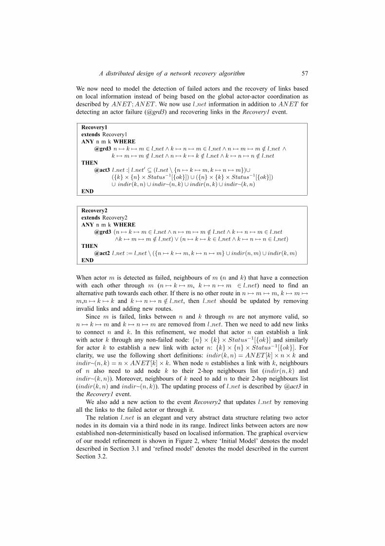
A distributed design of a network recovery algorithm 57
We now need to model the detection of failed actors and the recovery of links basedon local information instead of being based on the global actor-actor coordination asdescribed by ANET ; ANET . We now use l net information in addition to ANET fordetecting an actor failure (@grd3) and recovering links in the Recovery1 event.
Recovery1extends Recovery1ANY n m k WHERE
@grd3 n 7→ k 7→ m ∈ l net ∧ k 7→ n 7→ m ∈ l net ∧ n 7→ m 7→ m /∈ l net ∧k 7→ m 7→ m /∈ l net ∧ n 7→ k 7→ k /∈ l net ∧ k 7→ n 7→ n /∈ l net
THEN@act3 l net :| l net′ ⊆ (l net \ {n 7→ k 7→ m, k 7→ n 7→ m})∪
({k} × {n} × Status−1[{ok}]) ∪ ({n} × {k} × Status−1[{ok}])∪ indir(k, n) ∪ indir~(n, k) ∪ indir(n, k) ∪ indir~(k, n)
END
Recovery2extends Recovery2ANY n m k WHERE
@grd3 (n 7→ k 7→ m ∈ l net ∧ n 7→ m 7→ m /∈ l net ∧ k 7→ n 7→ m ∈ l net∧k 7→ m 7→ m /∈ l net) ∨ (n 7→ k 7→ k ∈ l net ∧ k 7→ n 7→ n ∈ l net)
THEN@act2 l net := l net \ ({n 7→ k 7→ m, k 7→ n 7→ m} ∪ indir(n, m) ∪ indir(k, m)
END
When actor m is detected as failed, neighbours of m (n and k) that have a connectionwith each other through m (n 7→ k 7→ m, k 7→ n 7→ m ∈ l net) need to find analternative path towards each other. If there is no other route in n 7→ m 7→ m, k 7→ m 7→m,n 7→ k 7→ k and k 7→ n 7→ n /∈ l net, then l net should be updated by removinginvalid links and adding new routes.
Since m is failed, links between n and k through m are not anymore valid, son 7→ k 7→ m and k 7→ n 7→ m are removed from l net. Then we need to add new linksto connect n and k. In this refinement, we model that actor n can establish a linkwith actor k through any non-failed node: {n} × {k} × Status−1[{ok}] and similarlyfor actor k to establish a new link with actor n: {k} × {n} × Status−1[{ok}]. Forclarity, we use the following short definitions: indir(k, n) = ANET [k]× n× k andindir~(n, k) = n×ANET [k]× k. When node n establishes a link with k, neighboursof n also need to add node k to their 2-hop neighbours list (indir(n, k) andindir~(k, n)). Moreover, neighbours of k need to add n to their 2-hop neighbours list(indir(k, n) and indir~(n, k)). The updating process of l net is described by @act3 inthe Recovery1 event.
We also add a new action to the event Recovery2 that updates l net by removingall the links to the failed actor or through it.
The relation l net is an elegant and very abstract data structure relating two actornodes in its domain via a third node in its range. Indirect links between actors are nowestablished non-deterministically based on localised information. The graphical overviewof our model refinement is shown in Figure 2, where ‘Initial Model’ denotes the modeldescribed in Section 3.1 and ‘refined model’ denotes the model described in the currentSection 3.2.

58 M. Kamali et al.
Figure 2 Overview of our model refinement
4 Distributing the recovery algorithm
In this section we put forward the decomposition of our centralised WSAN modelinto a model for a WSAN infrastructure and a model for the distributed actor node(s).The correctness of this decomposition step is addressed as a special kind of modelrefinement.
4.1 A distributed model of the actor network
In the initial model we capture the recovery algorithm in a centralised way. Thiscentralisation is achieved by allowing the actor nodes to access global network links,modelled by ANET . However, in the following refinement step, the variable l net isintroduced to limit the actor access to the local network links rather than the globalones. Such a refinement step allows us to express the distributed nature of the recoveryalgorithm in WSANs. Specifically, the refined model represents the communicatinginfrastructure together with actions of separate actors, so that everything is modelledin a single machine. On one hand, the modelling and the verification of properties inthe network is simpler but, on the other hand, it causes difficulties for its distributedimplementation. Therefore, in order to implement a distributed actor network, we needto separate the WSAN infrastructure and the individual actor operations.
The overall scheme of the decomposition refinement is shown in Figure 3. Themodel presented in Section 3.2 (‘refined model’ in Figure 3) is now split into twoparts: an interface model, named ‘Actor Interface’ and a machine model, named ‘WSANMiddleware’. The interface specifies the external state and the behaviour model ofactor nodes, while the machine models the WSAN infrastructure that enables the nodesto communicate with each other. The actor interface is imported into the machineas a module, which is indexed by the set of actor nodes. This machine acts as thecommunication middleware providing access to module instances via the given interface.
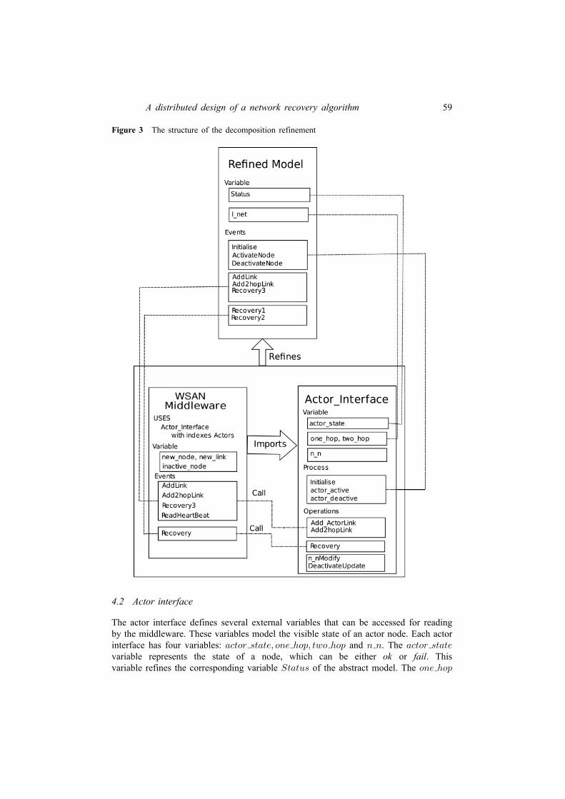
A distributed design of a network recovery algorithm 59
Figure 3 The structure of the decomposition refinement
4.2 Actor interface
The actor interface defines several external variables that can be accessed for readingby the middleware. These variables model the visible state of an actor node. Each actorinterface has four variables: actor state, one hop, two hop and n n. The actor statevariable represents the state of a node, which can be either ok or fail. Thisvariable refines the corresponding variable Status of the abstract model. The one hop
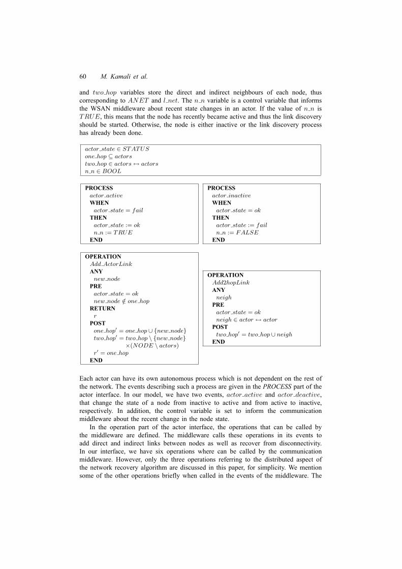
60 M. Kamali et al.
and two hop variables store the direct and indirect neighbours of each node, thuscorresponding to ANET and l net. The n n variable is a control variable that informsthe WSAN middleware about recent state changes in an actor. If the value of n n isTRUE, this means that the node has recently became active and thus the link discoveryshould be started. Otherwise, the node is either inactive or the link discovery processhas already been done.
actor state ∈ STATUSone hop ⊆ actorstwo hop ∈ actors ↔ actorsn n ∈ BOOL
PROCESSactor activeWHENactor state = fail
THENactor state := okn n := TRUE
END
PROCESSactor inactiveWHEN
actor state = okTHEN
actor state := failn n := FALSE
END
OPERATIONAdd ActorLinkANYnew node
PREactor state = oknew node /∈ one hop
RETURNr
POSTone hop′ = one hop ∪ {new node}two hop′ = two hop \ {new node}
×(NODE \ actors)r′ = one hop
END
OPERATIONAdd2hopLinkANY
neighPRE
actor state = okneigh ∈ actor ↔ actor
POSTtwo hop′ = two hop ∪ neigh
END
Each actor can have its own autonomous process which is not dependent on the rest ofthe network. The events describing such a process are given in the PROCESS part of theactor interface. In our model, we have two events, actor active and actor deactive,that change the state of a node from inactive to active and from active to inactive,respectively. In addition, the control variable is set to inform the communicationmiddleware about the recent change in the node state.
In the operation part of the actor interface, the operations that can be called bythe middleware are defined. The middleware calls these operations in its events toadd direct and indirect links between nodes as well as recover from disconnectivity.In our interface, we have six operations where can be called by the communicationmiddleware. However, only the three operations referring to the distributed aspect ofthe network recovery algorithm are discussed in this paper, for simplicity. We mentionsome of the other operations briefly when called in the events of the middleware. The
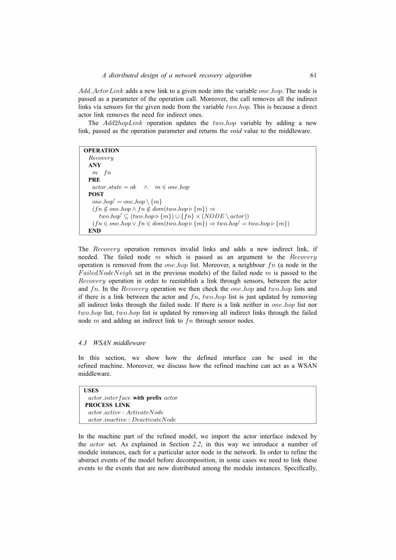
A distributed design of a network recovery algorithm 61
Add ActorLink adds a new link to a given node into the variable one hop. The node ispassed as a parameter of the operation call. Moreover, the call removes all the indirectlinks via sensors for the given node from the variable two hop. This is because a directactor link removes the need for indirect ones.
The Add2hopLink operation updates the two hop variable by adding a newlink, passed as the operation parameter and returns the void value to the middleware.
OPERATIONRecoveryANY
m fnPRE
actor state = ok ∧ m ∈ one hopPOST
one hop′ = one hop \ {m}(fn /∈ one hop ∧ fn /∈ dom(two hop ◃ {m}) ⇒
two hop′ ⊆ (two hop ◃ {m}) ∪ {fn} × (NODE \ actor))(fn ∈ one hop ∨ fn ∈ dom(two hop ◃ {m}) ⇒ two hop′ = two hop ◃ {m})
END
The Recovery operation removes invalid links and adds a new indirect link, ifneeded. The failed node m which is passed as an argument to the Recoveryoperation is removed from the one hop list. Moreover, a neighbour fn (a node in theFailedNodeNeigh set in the previous models) of the failed node m is passed to theRecovery operation in order to reestablish a link through sensors, between the actorand fn. In the Recovery operation we then check the one hop and two hop lists andif there is a link between the actor and fn, two hop list is just updated by removingall indirect links through the failed node. If there is a link neither in one hop list nortwo hop list, two hop list is updated by removing all indirect links through the failednode m and adding an indirect link to fn through sensor nodes.
4.3 WSAN middleware
In this section, we show how the defined interface can be used in therefined machine. Moreover, we discuss how the refined machine can act as a WSANmiddleware.
USESactor interface with prefix actorPROCESS LINKactor active : ActivateNodeactor inactive : DeactivateNode
In the machine part of the refined model, we import the actor interface indexed bythe actor set. As explained in Section 2.2, in this way we introduce a number ofmodule instances, each for a particular actor node in the network. In order to refine theabstract events of the model before decomposition, in some cases we need to link theseevents to the events that are now distributed among the module instances. Specifically,

62 M. Kamali et al.
ActivateNode and DeactivateNode are the abstract events that are linked to thecorresponding events in the process part of the actor interface.
One of the goals of the decomposition refinement step is data refinement of the datastructures modelling the actor coordination and recovery mechanism in WSANs by theones representing the coordination model of individual actors. Therefore, we need toshow that the one hop and two hop variables of the actor module instances are correctreplacements (i.e., data refinements) of the l net variable from the abstract model. Inaddition, the abstract Status variable is now data refined by actor state residing inmodule instances. The gluing invariants between abstract and concrete variables are asfollows:
l net = (id ▹ (one hop× one hop)) ∪ two hopstatus = actor state
The remaining events of the refined machine can be split into two groups. The firstgroup consists of a single (new) event describing how the middleware monitors the actornodes, specifically looking for new activated nodes or previously active and currentlyfailed nodes. The second group consists of several events specifying the middlewarereactions in response to the detected changes. The corresponding reactions are specifiedusing operation calls to the affected node instances. These events are refinements of theabstract events for adding new links and initiating the recovery mechanism.
EVENTSReadHeartBeatANY
n new failWHERE
n ∈ actors(n n(n) = TRUE ∧ new node = ∅ ∧ new = n) ∨ (new = ∅)(actor state(n) = fail ∧ one hop(n) = ∅ ∧ inactive node = ∅ ∧ fail = n)∨(fail = ∅)
THENnew node := newinactive node := failFailedNodeNeigh := DeactivateUpdate(fail)
END
The new monitoring event is called ReadHeartBeat. As node activation anddeactivation independently happens in a node and the network is not immediately awareof these changes, this event alarms the communication middleware for any changes inthe network topology. The detected changes are stored into two new variables new nodeand inactive node, which represent the indexes of, respectively, a node that wasrecently activated in the network and a node that recently failed (i.e., became inactive).In its guard, the ReadHeartBeat event checks the state of actor node instances. If then n value of the actor node is TRUE then new node is updated to the actor index.Moreover, if the actor state value of the actor is fail and one hop is not empty, i.e., theactor node has recently failed and recovery should be started, then the inactive nodevariable is also updated by the actor index. Finally, the DeactivateUpdate operationof the failed node is called to set the list of one− hop and two− hop with ∅ andreturn the neighbours of the node to update FailedNodeNeigh. When one− hop list

A distributed design of a network recovery algorithm 63
of a failed node is set to ∅ denotes that the node failure has been considered and therecovery links had been reestablished after detection of the failed node. Guards of theReadHeartBeat event corresponds to conditions that if a node has recently added orremoved from the network which are modelled by evaluating the value of n n andone hop in each node, repectively.
The second group of events consists of the events AddLink, Add2hopLink,and Recovery. The AddLink event is enabled when a new node joins the networkand an active actor is in its communication range. By calling the Actor AddLinkoperations of these two neighbours, the corresponding internal lists of 1-hop neighboursof these nodes are updated, while the lists of 2-hop neighbours are returned to theAddLink event. The returned lists are saved into two variables m neigh and n neighto be used in the Add2hopLink event to update the lists of 2-hop neighbours.Note the syntax of operation calls including two pairs of parentheses: in the firstparentheses, the index of a called node instance is given, while, within the secondparentheses, the concrete arguments of the procedure call are passed to the given moduleinstance.
In the Add2hopLink event, the Add2hopLink operation is called for differentmodule instances and their results are returned to the event. Since the return value of theAdd2hopLink operation is void, we have to assign it to the corresponding variables ofthe type V OID. However, for the sake of clarity, we introduce a shorthand notation forsuch calls: instead of void var := Operation(index) (parameters) we simply writeOperation (index) (parameters). Please also note that the module instance indexvalues used within operation calls in this event are actually not single values but setsof indexes. In such a way, we can specify a multiple (broadcasting) call, when thesame operations of a number of affected module instances are called simultaneously.Besides, the n nModify operation updates the value of n n from TRUE to FALSEand is called for new node. The n n variable of new node is updated to denote thatthe one hop and two hop lists of new node and its neighbours are updated. Updatingof n n variable in a node causes the communication middleware to not consider thenode as a new node anymore.
EVENTSAddLink
ANYn m
WHEREn ∈ new node
m ∈ actors ∧ n = m
dist(n 7→ m) < r a
THENm neigh :=(Actor AddLink(m)(n))×{m}n neigh :=(Actor AddLink(n)(m))×{n}new link := {n, m}END
EVENTSAdd2hopLink
ANYn m
WHEREn ∈ new node ∧m ∈ new link ∧ n = m
THENAdd2hopLink(dom(n neigh))({m 7→ n})Add2hopLink(dom(m neigh))({n 7→ m})Add2hopLink(dom(n))(m neigh)
Add2hopLink(dom(m))(n neigh)
new link := ∅new node := ∅n nModify(new node)
END
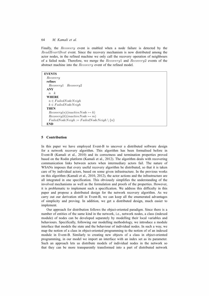
64 M. Kamali et al.
Finally, the Recovery event is enabled when a node failure is detected by theReadHeartBeat event. Since the recovery mechanism is now distributed among theactor nodes, in the refined machine we only call the recovery operation of neighboursof a failed node. Therefore, we merge the Recovery1 and Recovery2 events of theabstract machine into the Recovery event of the refined model.
EVENTSRecoveryrefines
Recovery1 Recovery2ANY
n kWHERE
n ∈ FailedNodeNeighk ∈ FailedNodeNeigh
THENRecovery(n)(inactiveNode 7→ k)Recovery(k)(inactiveNode 7→ m)FailedNodeNeigh := FailedNodeNeigh \ {n}
END
5 Contribution
In this paper we have employed Event-B to uncover a distributed software designfor a network recovery algorithm. This algorithm has been formalised before inEvent-B (Kamali et al., 2010) and its correctness and termination properties provedbased on the Rodin platform (Kamali et al., 2012). The algorithm deals with recoveringcommunication links between actors when intermediary actors fail. The nature ofWSANs imposes that every useful recovery algorithm be distributed, so that it is takencare of by individual actors, based on some given infrastructure. In the previous workson this algorithm (Kamali et al., 2010, 2012), the actor actions and the infrastructure areall integrated in one specification. This obviously simplifies the understanding of theinvolved mechanisms as well as the formulation and proofs of the properties. However,it is problematic to implement such a specification. We address this difficulty in thispaper and propose a distributed design for the network recovery algorithm. As wecarry out our derivation still in Event-B, we can keep all the enumerated advantagesof simplicity and proving. In addition, we get a distributed design, much easier toimplement.
Our approach for distribution follows the object-oriented paradigm. Since there is anumber of entities of the same kind in the network, i.e., network nodes, a class (indexedmodule) of nodes can be developed separately by modelling their local variables andbehaviours. Specifically, following our modelling methodology, we introduce a moduleinterface that models the state and the behaviour of individual nodes. In such a way, wemap the notion of a class in object-oriented programming to the notion of of an indexedmodule in Event-B. Similarly to creating new objects of a class in object-orientedprogramming, in our model we import an interface with an index set as its parameter.Such an approach lets us distribute models of individual nodes in the network sothat they can be more transparently transformed into a part of distributed network

A distributed design of a network recovery algorithm 65
implementation. The decomposed model provides enough intuition towards creatingobject-oriented code out of it.
Another interesting aspect of our derived distributed design refers to the failingactors. Actors can fail and be activated non-deterministically both in the integratedspecification and in the distributed one. In the integrated specification however, onlyone node could fail at a time and the algorithm takes care of recovering its neighbourscommunication. Only after that can the normal operation of the actor, including otherpossible actor failures, occur. In the distributed design, any number of actors canfail simultaneously or sequentially. The distributed recovery algorithm takes care ofrecovering the communication of each failed actor’s neighbours, in a non-deterministicorder and (still) one at a time. This is a significant reduction of the previous constraintsand constitutes an important contribution to modelling a reliable and more realisticdistributed recovery.
6 Related work and conclusions
Several formal developments of complex systems have used the Event-B formal method,for instance network protocols (Abrial et al., 2003; Rehm, 2010), network-on-chipmodelling (Kamali et al., 2011a, 2011b) and sensor networks (Kamali et al.,2010). Cansell and Mery (2006) model a development of a distributed referencecounting algorithm by using the refinement technique. Hoang et al. (2009) develop atopology discovery algorithm in Event-B, to prove safety and liveness properties. Themajor contribution in these formal models consists in developing correct-by-constructionmodels with the help of the refinement technique. Our contribution goes one step further,to decompose a verified development towards a distributed implementation.
Ball and Butler (2006) present a practical approach to the formal development ofmulti-agent systems in Event-B by using abstraction and decomposition techniques. Themain purpose of using the decomposition method for the development is to cope withthe complexity of the system. When the model is refined, it becomes more concreteand complex. Therefore, decomposition is ideal for simplifying the complexity of themodel. In comparison, our aim is to apply the decomposition technique to approach animplementation of a distributed system.
Iliasov et al. (2011) decompose an integrated correct-by-construction specification ofa distributed system to gain its distributed program. The paper addresses a state-basedformal approach to correct-by-construction development of distributed programs. Theauthors present their approach by developing of a distributed leader election protocolas a case study. Decomposition refinement in the case study is accomplished by twoinstances of the module interface while in this paper we use indexed instances andapproach an object-oriented implementation.
Ray and Cleaveland (2004) present a formal modelling of middleware-baseddistributed systems. They extend architectural integration diagrams (AIDs) (Ray andCleaveland, 2003) by providing an operational semantics that supports formal analysisof distributed system designs. AID provides a mechanism that supports a wide varietyof interprocess communication and frees the designers from manually modelling thedifferent interprocess communications. Another middleware-based systems formalism ispresented in Dan and Danning (2010). They work on semi-formal UML-based analysisusing UML profiles and a notion of behavioural semantics. The main purpose of these

66 M. Kamali et al.
studies is the proposal of an operational semantics for modelling middleware-baseddistributed systems to analyse different designs. In this paper, we understand themiddleware as a network infrastructure stepwise derived to achieve distribution.
The derivation of a distributed design from an integrated algorithm is very similarin nature to well-established research in formal methods, for instance in Back and Sere(1996). The derivation of a distributed broadcast algorithm from a centralised one isemployed there as a case study and the formal development is carried out in actionsystems (Back and Kurki-Suonio, 1983) instead of Event-B. It is worth mentioning thatactions systems are in fact a precursor of Event-B. However, Event-B has the associatedRodin platform, which makes proving an automated matter and thus brings a significantadvantage to the establishment of reliable practices in software development.
ReferencesAbrial, J-R., Cansell, D. and Mery, D. (2003) ‘A mechanically proved and incremental
development of IEEE 1394 tree identify protocol’, Formal Aspects of Computing,Vol. 14, No. 3, pp.215–227.
Abrial, J-R. (1996) The B-book: Assigning Programs to Meanings, Cambridge University Press,New York, NY, USA.
Abrial, J-R. (2001) ‘Event driven distributed program construction’, MATISSE project.Abrial, J-R. (2007) ‘A system development process with Event-B and the Rodin platform’,
in Butler, Michael, Hinchey, Michael, G. and Larrondo-Petrie, María, M. (Eds): FormalMethods and Software Engineering, Vol. 4789, pp.1–3, Springer Berlin Heidelberg.
Abrial, J-R. (2010) Modeling in Event-B – System and Software Engineering, CambridgeUniversity Press, New York, NY.
Akyildiz, I. and Kasimoglu, I. (2004) ‘Wireless sensor and actor networks: research challenges’,Ad Hoc Networks, Vol. 2, No. 4, pp.351–367.
Back, R. and Kurki-Suonio, R. (1983) ‘Decentralization of process nets with centralized control’,in Proceedings of the 2nd ACM SIGACT-SIGOPS Symposium on Principles of DistributedComputing, pp.131–142.
Back, R-J. and Sere, K. (1989) ‘Stepwise refinement of action systems’, inJ.L.A. van de Snepscheut (Ed.): Mathematics of Program Construction, 375th Anniversaryof the Groningen University, International Conference, Groningen, The Netherlands, June26–30, Vol. 375 of Lecture Notes in Computer Science, Springer, pp.115–138.
Back, R.J.R. and Sere, K. (1996) ‘Superposition refinement of reactive systems’, Formal Aspectsof Computing, Vol. 8, No. 3, pp.324–346.
Ball, E. and Butler, M. (2006) ‘Using decomposition to model multi-agent interaction protocolsin Event-B’, in FM ‘06 Doctoral Symposium, Springer.
Booch, G. (2007) ‘Speaking truth to power’, IEEE Software, Vol. 24, No. 2, pp.12–13.Cansell, D. and Mery, D. (2006) ‘Formal and incremental construction of distributed algorithms:
on the distributed reference counting algorithm’, Theoretical Computer Science, Vol. 364,No. 3, pp.318–337.
Dan, L. and Danning, L. (2010) ‘Towards a formal behavioral semantics for UML interactions’,in Information Science and Engineering (ISISE), 2010 International Symposium on,pp.213–218.
Fathabadi, M., Salehi, A., Rezazadeh, A. and Butler, M. (2011) ‘Applying atomicity andmodel decomposition to a space craft system in Event-B’, in M.G. Bobaru, K. Havelund,G.J. Holzmann and R. Joshi (Eds.): NASA Formal Methods, Vol. 6617 of Lecture Notes inComputer Science, pp.328–342, Springer.

A distributed design of a network recovery algorithm 67
Gerhart, S., Craigen, D. and Ralston, T. (1994) ‘Case study: Paris Metro signaling system’,Software, IEEE, Vol. 11, No. 1, pp.32–35.
Gungor, V.C., Akan, O.B. and Akyildiz, I.F. (2008) ‘A real-time and reliable transport (rt) 2protocol for wireless sensor and actor networks’, IEEE/ACM Trans. Netw., Vol. 16, No. 2,pp.359–370 [online] http://dx.doi.org/10.1109/TNET.2007.900413.
Hoang, T., Kuruma, H., Basin, D.A. and Abrial, J-R. (2009) ‘Developing topology discovery inEvent-B’, in IFM, pp.1–19.
Iliasov, A., Troubitsyna, E., Laibinis, L., Romanovsky, A., Varpaaniemi, K., Ilic, D. andLatvala, T. (2010) ‘ Supporting reuse in event-b development: modularisation approach’,in ASM ‘10, pp.174–188.
Iliasov, A., Troubitsyna, E., Laibinis, L. and Romanovsky, A. (2011) ‘Formal derivation of adistributed program in Event-B’, in ICFEM ‘11, LNCS, pp.420–436.
Imran, M., Younis, M., Said, A.M. and Hasbullah, H. (2012) ‘Localized motion-basedconnectivity restoration algorithms for wireless sensor and actor networks’,Journal of Network and Computer Applications, Vol. 35, No. 2, pp.844–856 [online]http://www.sciencedirect.com/science/article/pii/S1084804511002347(accessed 22 January 2013).
Jeremy, B. and Wei, W. (2010) ‘Formal analysis of BPMN models using Event-B’,in S. Kowalewski and M. Roveri (Eds.): Formal Methods for Industrial CriticalSystems – 15th International Workshop, FMICS 2010, Vol. 6371 of Lecture Notes inComputer Science, pp.33–49, Antwerp, Belgium, September 20–21, Springer.
Kamali, M., Sedighian, S. and Sharifi, M. (2008) ‘A distributed recovery mechanismfor actor-actor connectivity in wireless sensor actor networks’, in Intelligent Sensors,Sensor Networks and Information Processing, ISSNIP 2008, International Conference on,pp.183–188.
Kamali, M., Laibinis, L., Petre, L. and Sere, K. (2010) ‘Self-recovering sensor-actor networks’,in FOCLASA, pp.47–61.
Kamali, M., Petre, L., Sere, K. and Daneshtalab, M. (2011a) ‘Formal modeling of multicastcommunication in 3D NoCs’, in Digital System Design (DSD), 2011 14th EuromicroConference on, pp.634 –642.
Kamali, M., Petre, L., Sere, K. and Daneshtalab, M. (2011b) ‘Refinement-based modeling of3D NoCs’, in Fundamental of Software Engineering (FSEN), 2011 4th IPM InternationalConference on.
Kamali, M., Laibinis, L., Petre, L. and Sere, K. (2012) ‘Formal development ofwireless sensor-actor networks’, Science of Computer Programming [online]http://www.sciencedirect.com/science/article/pii/S0167642312000470?v=s5(accessed 22 January 2013).
Katz, S. (1993) ‘A superimposition control construct for distributed systems’, ACM Trans.Program. Lang. Syst., Vol. 15, No. 2, pp.337–356.
Lecomte, T. (2009) ‘Applying a formal method in industry: a 15-year trajectory’, in Proceedingsof the 14th International Workshop on Formal Methods for Industrial Critical Systems,FMICS ‘09, Springer-Verlag, Berlin, Heidelberg, pp.26–34.
Ngai, E.C.H., Lyu, M.R. and Liu, J. (2006) ‘A real-time communication framework for wirelesssensor-actuator networks’, in Proc. of the IEEE Aerospace Conference, Big Sky.
Ray, A. and Cleaveland, R. (2003) ‘Architectural interaction diagrams: AIDs for systemmodeling’, in Software Engineering, Proceedings. 25th International Conference on,pp.396–406.
68 M. Kamali et al.
Ray, A. and Cleaveland, R. (2004) ‘Formal modeling of middleware-based distributedsystems’, Electron. Notes Theor. Comput. Sci., Vol. 108, No. 1, pp.21–37 [online]http://dx.doi.org/10.1016/j.entcs.2004.01.010 (accessed 22 January 2013).
Rehm, J. (2010) ‘Proved development of the real-time properties of the IEEE 1394 rootcontention protocol with the Event-B method’, International Journal on Software Tools forTechnology Transfer, Vol. 12, No. 1, pp.39–51.
Rodin Modularisation Plug-in (2011) [online]http://wiki.event-b.org/index.php/Modularisation Plug-in/ (accessed 26 October 2011).
Rodin Tool Platform (2006) [online] http://www.event-b.org/platform.html/(accessed 26 October 2011).
Woodcock, J., Larsen, P., Bicarregui, J. and Fitzgerald, J. (2009) ‘Formal methods: practice andexperience’, ACM Comput. Surv., Vol. 41, No. 4, pp.1–36.

Paper III
Topology-based Mobility Model for Wireless
Networks
Ansgar Fehnker, Peter Höfner, Maryam Kamali and
Vinay Mehta
Originally published in: K. Joshi et al. (Eds.), Proceedings of the 10th In-ternational Conference on Quantitative Evaluation of Systems conference -QEST 13, Lecture Notes in Computer Science Vol. 8054, pp. 389-404,Springer-Verlag, 2013.
101

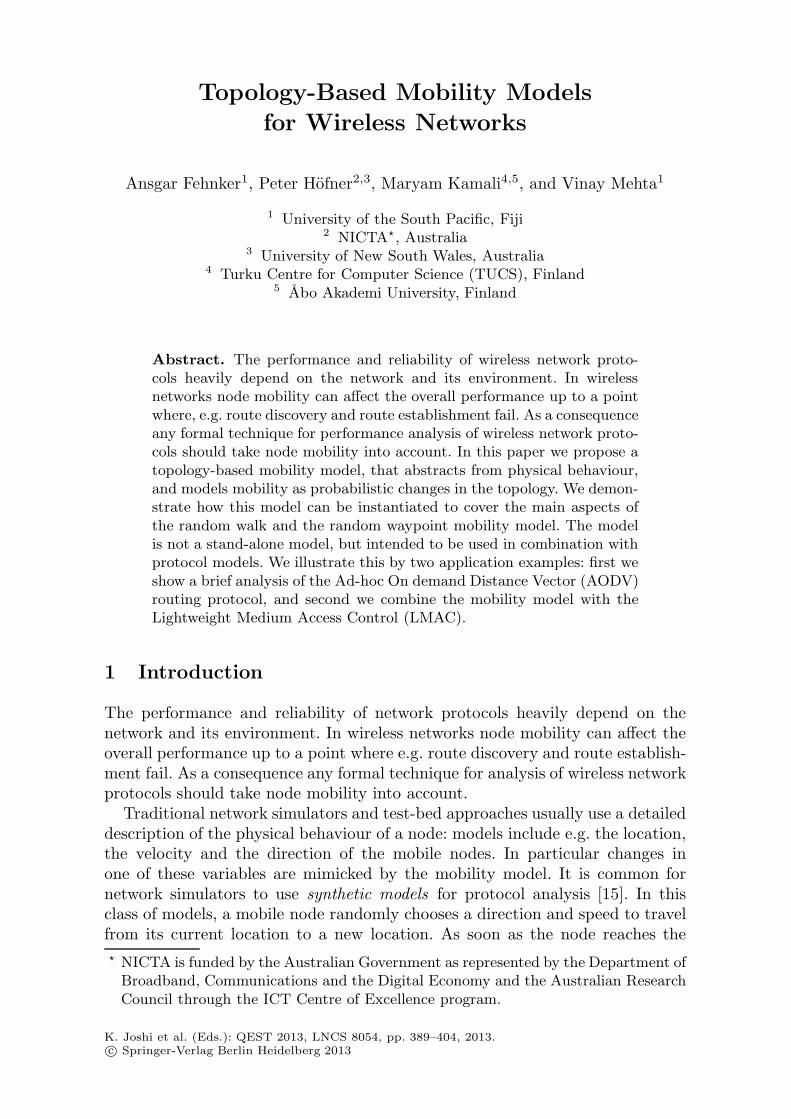
Topology-Based Mobility Models
for Wireless Networks
Ansgar Fehnker1, Peter Hofner2,3, Maryam Kamali4,5, and Vinay Mehta1
1 University of the South Pacific, Fiji2 NICTA�, Australia
3 University of New South Wales, Australia4 Turku Centre for Computer Science (TUCS), Finland
5 Abo Akademi University, Finland
Abstract. The performance and reliability of wireless network proto-cols heavily depend on the network and its environment. In wirelessnetworks node mobility can affect the overall performance up to a pointwhere, e.g. route discovery and route establishment fail. As a consequenceany formal technique for performance analysis of wireless network proto-cols should take node mobility into account. In this paper we propose atopology-based mobility model, that abstracts from physical behaviour,and models mobility as probabilistic changes in the topology. We demon-strate how this model can be instantiated to cover the main aspects ofthe random walk and the random waypoint mobility model. The modelis not a stand-alone model, but intended to be used in combination withprotocol models. We illustrate this by two application examples: first weshow a brief analysis of the Ad-hoc On demand Distance Vector (AODV)routing protocol, and second we combine the mobility model with theLightweight Medium Access Control (LMAC).
1 Introduction
The performance and reliability of network protocols heavily depend on thenetwork and its environment. In wireless networks node mobility can affect theoverall performance up to a point where e.g. route discovery and route establish-ment fail. As a consequence any formal technique for analysis of wireless networkprotocols should take node mobility into account.
Traditional network simulators and test-bed approaches usually use a detaileddescription of the physical behaviour of a node: models include e.g. the location,the velocity and the direction of the mobile nodes. In particular changes inone of these variables are mimicked by the mobility model. It is common fornetwork simulators to use synthetic models for protocol analysis [15]. In thisclass of models, a mobile node randomly chooses a direction and speed to travelfrom its current location to a new location. As soon as the node reaches the� NICTA is funded by the Australian Government as represented by the Department of
Broadband, Communications and the Digital Economy and the Australian ResearchCouncil through the ICT Centre of Excellence program.
K. Joshi et al. (Eds.): QEST 2013, LNCS 8054, pp. 389–404, 2013.c© Springer-Verlag Berlin Heidelberg 2013

390 A. Fehnker et al.
new location, it randomly chooses the next direction. Although these modelsabstract from certain characteristics such as acceleration, they still cover mostof the physical attributes of the mobile node. Two well-known synthetic mobilitymodels are the random walk (e.g. [1]) and the random waypoint model (e.g. [2]).
However, a physical mobility model is often incompatible with models of pro-tocols, in particular protocols in the data link and network layers, due to lim-itations of the used modeling language and analysis tools. Even if it could beincluded, it would add a high complexity and make automatic analysis infeasible.From the point of view of the protocol it is often sufficient to model changes onthe topology (connectivity matrix) rather than all physical behaviour.
In this paper we propose a topology-based mobility model that abstractsfrom physical behaviour, and models mobility as probabilistic changes in thetopology. The main idea is to identify the position of a node with its current setof neighbours and determine changes in the connectivity matrix by adding ordeleting nodes probabilistically to this set. The probabilities are distilled fromthe random walk or the random waypoint model. The resulting model is notmeant to be a stand-alone model, but to be used in combination with protocolmodels. For this, we provide an Uppaal template for our model, which can easilybe added to existing protocol models. The paper illustrates the flexibility of ourmodel by two application examples: the first analyses quantitative aspects ofthe Ad hoc On-Demand Distance Vector (AODV) protocol [14], a widely usedrouting protocol, particularly tailored for wireless networks; the second examplepresents an analysis of the Lightweight Media Access Control (LMAC) [12], aprotocol designed for sensor networks to schedule communication, and targetedfor distributed self-configuration, collision avoidance and energy efficiency.
The rest of the paper is organised as follows: after a short overview of re-lated work (Sect. 2), we develop the topology-based mobility model in Sect. 3.In Sect. 4 we present a simulator that is used to compute the transition prob-abilities for two common mobility models. In Sect. 5, we combine the distilledprobabilities with our topology-based model to create an Uppaal model. Beforeconcluding in Sect. 7, we illustrate how the model can be used in conjunctionwith protocol models. More precisely we present a short analysis of AODV andLMAC.
2 Related Work
Mobility models are part of most network simulators such as ns-2. In contrast tothis, formal models used for verification or performance analysis usually assumea static topology, or consider a few scenarios with changing topology only. Forthe purpose of this section, we distinguish two research areas: mobility modelsfor network simulators and models for formal verification methods.
Mobility models for network simulators either replay traces obtained from realworld, or they use synthetic models, which abstract from some details and gen-erate mobility scenarios. There are roughly two dozen different synthetic models(see [15,4] for an overview), starting from well-known models such as the random
Topology-Based Mobility Models for Wireless Networks 391
walk model (e.g. [1]) and the random way point model (e.g. [2]), via (partially)deterministic models and Manhattan models to Gauss-Markov and gravity mo-bility models. All these models are based on the physical behaviour of mobilenodes, i.e. each node has a physical location (in 2D or 3D1), a current speedand a direction it is heading to. As these models cover most of the physical be-haviour, they are most often very complex (e.g. [13,10]) and include for examplemathematics for Brownian motion. Due to this complexity these models cannotbe incorporated directly into formal models for model-checking. This paper de-scribes how two of these models, the random waypoint, and the random walkmodel, can be used to distill transition probabilities for a mobility model, whichcan easily be combined with formal protocol models.
Including mobility into a model for formal verification is not as common asit is for network simulators. If they are included, then typically in the protocolspecification and therefore can rarely be reused for the analysis of different pro-tocols. Moreover, formal verification often abstracts entirely from the underlyingmobility model and allows arbitrary topology changes [9,5,8]. Other approachesallow only random, but very limited changes in the topology, often in the form ofa scenario that involves deletion or creation of links [6,18,17]. Song and Godske-sen propose in [16] a framework for modelling mobility; it models connectivityby distributions and propose a probabilistic mobility function to model mobility,without any specifics. This paper takes a similar approach, but adjacency matri-ces to model connectivity, and works out and analyses the transition probabilitiesobtained for two mobility models.
Our contribution is the following: we take the idea that the position of amobile node can be characterised by a set of neighbours, which determines thetopology, and we then define mobility as transitions between these sets. We thenanalyse the geometry of mobile nodes in a grid and determine which parametersactually influence the transition probabilities. In fact we found that some pa-rameters, such as the step size of the random walk model have no influence onthe transition probabilities. Based on this observation we build a topology-basedmobility model which can easily be combined with protocol models.
3 Topology-Based Mobility Model
Our model takes up the position of the protocol: for a protocol it only matterswhether data packets can be sent to a node, i.e. whether the node is withintransmission range. The speed, the direction and other physical attributes areunimportant and irrelevant for the protocol. Hence the topology-based mobilitymodel we introduce abstracts from all physical description of a node, and alsolargely abstracts from time. It models the node as a set of one-hop neighbours,i.e. nodes that are within transmission range of the node. Movement is modelledas a transition from one set of neighbours to another.
We assume that the node to be modelled moves within a quadratic N ×N -grid of stationary nodes. For simplicity we assume that nodes in the grid have a1 3D is required when nodes model aerospace vehicles, such as UAVs.

392 A. Fehnker et al.
R=1
R=1.12
R=1.18
R=1.25
R=1.41
Fig. 1. Transmission ranges 1,√
52
≈ 1.12, 56
√2≈ 1.18, 1.25 and
√2≈ 1.41
distance of 1, and that both the stationary and the mobile node have the sametransmission range R. Obviously, the model depends on the grid size and thetransmission range. We further assume that the transition range R is larger than1 and strictly smaller than
√2. If it were smaller than 1 nodes in the grid would
be outside of the range of all neighbours, if it were larger than√
2 nodes couldcommunicate diagonally in the grid.
The network topology of all nodes, including the mobile node, can be repre-sented by an adjacency or connectivity matrix A with
Ai,j ={
1 if D(i, j) ≤ R0 otherwise ,
where D(i, j) is the distance between the nodes i and j using some kind ofmetric, such as the Euclidean distance. While the connectivity matrix has theo-retically 2N2
possible configurations, with N the number of nodes, a networkwith one mobile node will only reach a small fraction of those. First, the matrixis symmetric. Second, all nodes, except for one, are assumed static, and theconnectivity Ai,j between two static nodes i and j will be constant. Third, dueto the geometry of the plane, even the mobile node can only have a limitednumber of configurations. For example, neither a completely connected node,nor a completely disconnected node is possible given the transmission range.
The possible topologies depend on the transmission range: the larger the rangethe larger the number of possible nodes that can be connected to the mobile node.Within the right-open interval [1,
√2), the set of possible topologies changes at
values√
52 , 5
6
√2 and 1.25. These values can be computed with basic trigonometry.
Fig. 1 illustrates which topologies become possible at those transmission ranges.By considering the transmission range of the stationary nodes, one can par-
tition the plane into regions in which mobile nodes will have the same set ofneighbours. The boundaries of these regions are defined by circles with radius Raround the stationary nodes. Fig. 2 depicts three possible regions and a trans-mission range R = 1.25; stationary nodes that are connected to the mobile node(located somewhere in the coloured area) are highlighted. As convention we willnumber nodes from the top left corner, starting with node 0. This partitioningabstracts from the exact location of the mobile node. Mobility can now be ex-pressed as a change from one region to the next. The topology-based model willcapture the changing topology as a Markovian transition function, that assignsto a pair of topologies a transition probability.
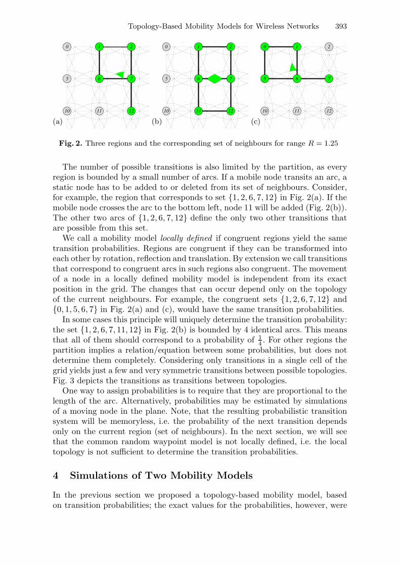
Topology-Based Mobility Models for Wireless Networks 393
(a)
121110
765
210
(b)
121110
765
210
(c)
121110
765
210
Fig. 2. Three regions and the corresponding set of neighbours for range R = 1.25
The number of possible transitions is also limited by the partition, as everyregion is bounded by a small number of arcs. If a mobile node transits an arc, astatic node has to be added to or deleted from its set of neighbours. Consider,for example, the region that corresponds to set {1, 2, 6, 7, 12} in Fig. 2(a). If themobile node crosses the arc to the bottom left, node 11 will be added (Fig. 2(b)).The other two arcs of {1, 2, 6, 7, 12} define the only two other transitions thatare possible from this set.
We call a mobility model locally defined if congruent regions yield the sametransition probabilities. Regions are congruent if they can be transformed intoeach other by rotation, reflection and translation. By extension we call transitionsthat correspond to congruent arcs in such regions also congruent. The movementof a node in a locally defined mobility model is independent from its exactposition in the grid. The changes that can occur depend only on the topologyof the current neighbours. For example, the congruent sets {1, 2, 6, 7, 12} and{0, 1, 5, 6, 7} in Fig. 2(a) and (c), would have the same transition probabilities.
In some cases this principle will uniquely determine the transition probability:the set {1, 2, 6, 7, 11, 12} in Fig. 2(b) is bounded by 4 identical arcs. This meansthat all of them should correspond to a probability of 1
4 . For other regions thepartition implies a relation/equation between some probabilities, but does notdetermine them completely. Considering only transitions in a single cell of thegrid yields just a few and very symmetric transitions between possible topologies.Fig. 3 depicts the transitions as transitions between topologies.
One way to assign probabilities is to require that they are proportional to thelength of the arc. Alternatively, probabilities may be estimated by simulationsof a moving node in the plane. Note, that the resulting probabilistic transitionsystem will be memoryless, i.e. the probability of the next transition dependsonly on the current region (set of neighbours). In the next section, we will seethat the common random waypoint model is not locally defined, i.e. the localtopology is not sufficient to determine the transition probabilities.
4 Simulations of Two Mobility Models
In the previous section we proposed a topology-based mobility model, basedon transition probabilities; the exact values for the probabilities, however, were

394 A. Fehnker et al.
Fig. 3. Possible transitions within a single grid cell for R =1.25
not specified. In this section we use a simulator to compute it for two commonmobility models, a random walk model, and a random waypoint model.
4.1 Simulator
The simulator considers a single mobile node in an N ×N grid of stationarynodes. As before, we assume a distance of 1 between the nodes on the grid. Theinitial position (x0, y0) of the mobile node is determined by a uniform distributionover [0, N − 1]×[0, N − 1], i.e. x0∼U([0, N − 1]) and y0∼U([0, N − 1]). Dependingon the mobility model chosen, the simulator then selects a finite number ofwaypoints (x1, y1), . . . , (xn, yn), and moves along a straight line from waypoint(xi, yi) to the next (xi+1, yi+1).
The random waypoint model uses a uniform distribution over the grid toselect the next way point, i.e. for all xi, we have yi, xi ∼ U([0, N − 1]) andyi ∼ U([0, N − 1]). The choice of the next waypoint is independent of the pre-vious waypoint. This model is the most common model of mobility for networksimulators, even if its merits have been debated [19]. A consequence of the way-point selection is that the direction of movement is not uniformly distributed;nodes tend to move more towards the centre of the square interval.
As an alternative we are using a simple random walk model. Given way point(xi, yi) the next way point is computed by (xi, yi) + (xΔ, yΔ) where both xΔ
and xΔ are drawn from a normal distribution N (0, σ). This also means that theEuclidean distance between waypoints ||(xΔ, yΔ)|| has an expected value of σ,which defines the average step size in the random walk model. By this definition,the model is unbounded, i.e. the next waypoint may lie outside the grid. If thishappens the simulator computes the intersection of the line segment with thegrid’s boundary and reflects the waypoint at that boundary. In this model themobile node moves from the first waypoint to the boundary, and from there tothe reflected waypoint. For the purposes of this paper the intersections with theboundary do not count as waypoints.
Since the topology-based mobility model introduced in Sect. 3 abstracts fromacceleration and speed, these aspects are not included in the simulation ei-ther. The simulator checks algebraically for every line segment from (xi, yi) to
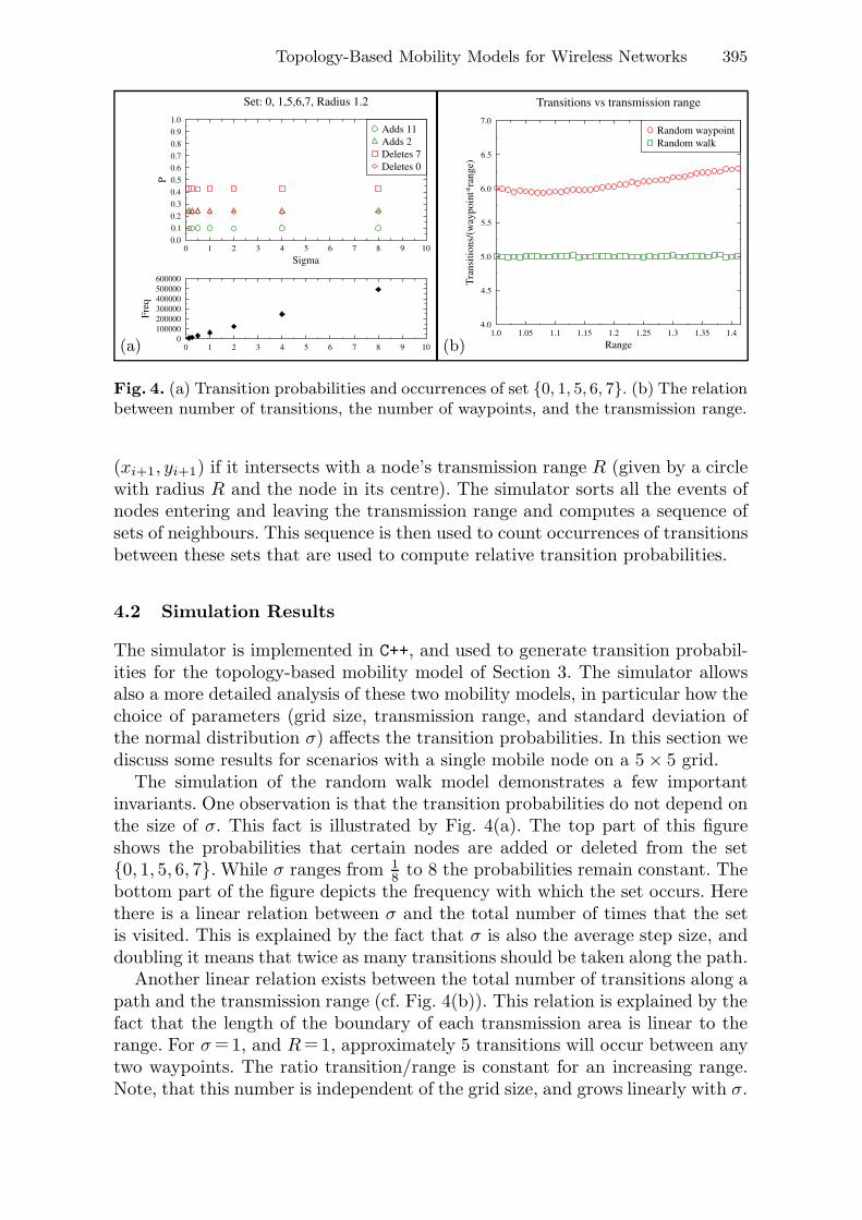
Topology-Based Mobility Models for Wireless Networks 395
(a)0
100000200000300000400000500000600000
Freq
0 1 2 3 4 5 6 7 8 9 10
0.0
0.1
0.2
0.3
0.4
0.5
0.6
0.7
0.8
0.9
1.0
P
0 1 2 3 4 5 6 7 8 9 10
Sigma
Set: 0, 1,5,6,7, Radius 1.2
Adds 11Adds 2Deletes 7Deletes 0
(b)
4.0
4.5
5.0
5.5
6.0
6.5
7.0
Transition
s/(w
aypo
int*rang
e)
1.0 1.05 1.1 1.15 1.2 1.25 1.3 1.35 1.4
Range
Transitions vs transmission range
Random waypointRandom walk
Fig. 4. (a) Transition probabilities and occurrences of set {0, 1, 5, 6, 7}. (b) The relationbetween number of transitions, the number of waypoints, and the transmission range.
(xi+1, yi+1) if it intersects with a node’s transmission range R (given by a circlewith radius R and the node in its centre). The simulator sorts all the events ofnodes entering and leaving the transmission range and computes a sequence ofsets of neighbours. This sequence is then used to count occurrences of transitionsbetween these sets that are used to compute relative transition probabilities.
4.2 Simulation Results
The simulator is implemented in C++, and used to generate transition probabil-ities for the topology-based mobility model of Section 3. The simulator allowsalso a more detailed analysis of these two mobility models, in particular how thechoice of parameters (grid size, transmission range, and standard deviation ofthe normal distribution σ) affects the transition probabilities. In this section wediscuss some results for scenarios with a single mobile node on a 5 × 5 grid.
The simulation of the random walk model demonstrates a few importantinvariants. One observation is that the transition probabilities do not depend onthe size of σ. This fact is illustrated by Fig. 4(a). The top part of this figureshows the probabilities that certain nodes are added or deleted from the set{0, 1, 5, 6, 7}. While σ ranges from 1
8 to 8 the probabilities remain constant. Thebottom part of the figure depicts the frequency with which the set occurs. Herethere is a linear relation between σ and the total number of times that the setis visited. This is explained by the fact that σ is also the average step size, anddoubling it means that twice as many transitions should be taken along the path.
Another linear relation exists between the total number of transitions along apath and the transmission range (cf. Fig. 4(b)). This relation is explained by thefact that the length of the boundary of each transmission area is linear to therange. For σ =1, and R = 1, approximately 5 transitions will occur between anytwo waypoints. The ratio transition/range is constant for an increasing range.Note, that this number is independent of the grid size, and grows linearly with σ.

396 A. Fehnker et al.
Random Walk Random Waypoint
05000
100001500020000250003000035000
Freq
1.0 1.05 1.1 1.15 1.2 1.25 1.3 1.35 1.4
Radius
0.0
0.1
0.2
0.3
0.4
0.5
0.6
0.7
0.8
0.9
1.0
P
1.0 1.05 1.1 1.15 1.2 1.25 1.3 1.35 1.4
Radius
Set: 1,2,6,7,11,12,
Adds 5Adds 8Deletes 2Deletes 11Deletes 12Deletes 1
(a)0
100002000030000400005000060000700008000090000
Freq
1.0 1.05 1.1 1.15 1.2 1.25 1.3 1.35 1.4
Radius
0.0
0.1
0.2
0.3
0.4
0.5
0.6
0.7
0.8
0.9
1.0
P
1.0 1.05 1.1 1.15 1.2 1.25 1.3 1.35 1.4
Radius
Set: 1,2,6,7,11,12,
Adds 5Adds 8Deletes 2Deletes 11Deletes 12Deletes 1
(b)
0
5000
10000
15000
20000
25000
Freq
1.0 1.05 1.1 1.15 1.2 1.25 1.3 1.35 1.4
Radius
0.0
0.1
0.2
0.3
0.4
0.5
0.6
0.7
0.8
0.9
1.0
P
1.0 1.05 1.1 1.15 1.2 1.25 1.3 1.35 1.4
Radius
Set: 2,6,7,12,
Adds 8Adds 11Adds 1Deletes 2Deletes 12
(c)0
10000
20000
30000
40000
50000
60000
Freq
1.0 1.05 1.1 1.15 1.2 1.25 1.3 1.35 1.4
Radius
0.0
0.1
0.2
0.3
0.4
0.5
0.6
0.7
0.8
0.9
1.0
P
1.0 1.05 1.1 1.15 1.2 1.25 1.3 1.35 1.4
Radius
Set: 2,6,7,12,
Adds 8Adds 11Adds 1Deletes 2Deletes 12
(d)
0
5000
10000
15000
20000
25000
Freq
1.0 1.05 1.1 1.15 1.2 1.25 1.3 1.35 1.4
Radius
0.0
0.1
0.2
0.3
0.4
0.5
0.6
0.7
0.8
0.9
1.0
P
1.0 1.05 1.1 1.15 1.2 1.25 1.3 1.35 1.4
Radius
Set: 1,5,6,7,
Adds 2Adds 11Adds 0Deletes 5Deletes 7
(e)0
500010000150002000025000300003500040000
Freq
1.0 1.05 1.1 1.15 1.2 1.25 1.3 1.35 1.4
Radius
0.0
0.1
0.2
0.3
0.4
0.5
0.6
0.7
0.8
0.9
1.0
P
1.0 1.05 1.1 1.15 1.2 1.25 1.3 1.35 1.4
Radius
Set: 1,5,6,7,
Adds 2Adds 11Adds 0Deletes 5Deletes 7
(f)
Fig. 5. Selected simulation results of the random walk and the random waypoint model

Topology-Based Mobility Models for Wireless Networks 397
These invariants do not hold for the random waypoint model. The ratio oftransitions to range is not constant, as illustrated in Fig. 4(b). This is becausetransitions are not evenly distributed but cluster towards the center of the grid.The ratio is also dependent on the size of the grid. In a larger grid the distancebetween waypoints will be larger, and more transitions occur per waypoint.
For the random walk model we found that the step size σ has no effect onthe actual transition probabilities. The effect of the transmission range on thetransition probabilities is less trivial. Fig. 5 shows a few illustrative examples.Similar result were obtained for all possible sets of neighbours.
Fig. 5(a) depicts the results for {1, 2, 6, 7, 11, 12}, a set of six nodes that forma rectangle. This set cannot occur if the transmission ranges are smaller than
√5
2(cf. Sect. 3). For transmission ranges R ∈ [
√5
2 , 1.25] the only possible transitionsare to delete one of the four vertices located at the corners of the rectangle. Inthe random walk model the probability for these four transitions is 1
4 . Fig. 5(a)also illustrates that for transmission ranges R≥ 1.25, it is possible to add oneadditional node (either 5 or 8), reaching a set with 7 one-hop neighbours. As therange increases, the probability of this happening increases. At the same timethe probability of deleting a vertex decreases.
Fig. 5(b) consider the same set of neighbours as Fig. 5(a), but under therandom waypoint model. It demonstrates that this model is not locally defined,as congruent transitions, e.g. deleting vertices, do not have the same probability.The probability also depends of the distance of a node to the centre of the grid.
Fig. 5(c–f) show the transition probabilities for sets of neighbours that occuronly if R∈[1, 1.25]: if R < 1, the transmission range is too small to cover thesets {2, 6, 7, 12} and {1, 5, 6, 7}, resp.; if R > 1.25 the transmission range of themobile will always contain more than four nodes. The observation is that as thetransmission range increases, the probability of deleting a node decreases, whilethe probability of adding nodes increases. The sets {2, 6, 7, 12} and {1, 5, 6, 7}have the same basic “�” shape; one is congruent to the other. Hence, for therandom walk model both sets have essentially the same transition probability;but also the frequency with which the sets occur is the same. This confirms thatthe position or orientation in the grid does not matter.
For the random waypoint model this no longer holds. The transition proba-bilities of similarly shaped neighbourhoods are not similar, but also determinedby the position relative to the centre: the closer the set is to the centre the oftenit occurs in paths. Note, Fig. 1(d) and (f) use different scales for the frequency.
To conclude this section, we summarise our findings:
Random walk model:
– The transition probabilities are independent of σ and the grid size;– The number of transitions per waypoint path grows linear with the range;– The transition probabilities of congruent transitions are the same;– The probabilities depend only locally on the set of nodes within range.
Random waypoint model: None of the above observations hold.

398 A. Fehnker et al.
Table 1. Number of possible topologies, in relation to the range and the grid size2
Transmission range[1, 1] (1, 1.12) (1.12, 1.18) (1.18, 1.25) [1.25, 1.25] (1.25, 1.41)
Gri
dsi
ze
2 × 2 9 9 5 5 5 53 × 3 32 41 49 49 37 414 × 4 69 97 133 133 101 1175 × 5 120 177 257 257 197 2336 × 6 185 281 421 421 325 3897 × 7 264 409 625 625 485 5858 × 8 357 561 869 869 677 8219 × 9 464 737 1153 1153 901 1097
10 × 10 585 937 1477 1477 1157 1413
5 Uppaal Model
This section describes an Uppaal model that implements the topology-basedmobility model described in Sect. 3, and uses the transition probabilities ob-tained in Sect. 4. The model is not meant to be stand-alone, but meant tobe used within other protocol models. It assumes that an adjacency matrixbool topoloy[N][N] is used. The constant N is the size of the grid plus the mo-bile node. Depending on whether the random walk or random waypoint modelis used, the model includes parameters for grid size and transmission range.
The template provides a list of all possible sets of neighbours. Table 1 showsthe numbers of possible sets depending on the size of the grid and the transmis-sion range. The results show that even for relatively large grids the number ofpossible sets of neighbors of the mobile node is limited. They will increase thepotential state space only by three order of magnitude. The reachable space mayincrease by more when a template for mobility is added, because the protocolmight reach more states than it did for static topologies.
The Uppaal template of Fig. 6 implements a lookup table of transition proba-bilities. After initialisation the template loops through a transition that changesthe topology probabilistically. It contains a clock t, a guard t>=minframe and aninvariant t<=maxframe to ensure that the change happens once in the interval[minframe,maxframe]. The values of minframe and maxframe determine thefrequency of topology changes, and hence simulate the speed of a node.
The lookup is implemented by functions updatemapindex, changeprob andchangenode. After every topology change, the function updatemapindex main-tains the index (mapindex); this index into the list of possible sets is used to lookup transition probabilities for a smaller set of representative sets of neighbours.Every set of neighbours is congruent to one of these representative sets. Thisinformation is used by changeprob to look up for a given node i the probabilitythat it will be added or deleted from the current set of neighbours. Functionchangenode implements that change.
2 Results for the point intervals containing√
52
and 56
√2 are omitted.

Topology-Based Mobility Models for Wireless Networks 399
t<=maxframe t>=minframe&& mapindex>=0 && numnodes<=MAXLENGTH
intitialiseN(),updatemapindex()
changenode(i),updatemapindex()
changeprob(i)i: int[0,NODES-2]
t=0
Fig. 6. Uppaal template for the mobility model
6 Application Examples
In this section we illustrate how the topology-based model can be used in com-bination with protocol models: first we briefly present an analysis of the Ad-hocOn demand Distance Vector (AODV) routing protocol, and second we combinethe mobility model with the Lightweight Medium Control (LMAC). A detailedstudy of these protocols is out of the scope of the paper; we only show theapplicability and power of the introduced mobility model.
Since we are interested in quantitative properties of the protocols, we arenot using “classical” Uppaal, but SMC-Uppaal, the statistical extension of Up-paal [3]. Statistical Model Checking (SMC) [20] combines ideas of model checkingand simulation with the aim of supporting quantitative analysis as well as ad-dressing the size barrier that currently prevents useful analysis of large models.SMC trades certainty for approximation, using Monte Carlo style sampling, andhypothesis testing to interpret the results. Parameters setting thresholds on theprobability of false negatives and on probabilistic uncertainty can be used tospecify the statistical confidence on the result. For this paper, we choose a con-fidence level of 95%.
6.1 The Ad-Hoc on Demand Distance Vector (AODV) Protocol
AODV is a reactive routing protocol, which means that routes are only estab-lished on demand. If a node S needs to send a data packet to node D, but cur-rently does not know a route, it buffers the packet and initiates a route discoveryprocess by broadcasting a route request message in the network. An intermediatenode A that receives this message stores a route to S, and re-broadcasts the re-quest. This is repeated until the message reaches D, or alternatively a node witha route to D. In both cases, the node replies to the route request by unicastinga route reply back to the source S, via the previously established route.
An Uppaal model of AODV is proposed in [6]. The analysis performed on thismodel was done for static topologies and for topologies with very few changes.This limits the scope of the performance analysis. Here, the mobility automatonis added to the model of AODV. Since the mobility automaton is an almostindependent component, it can be easily integrated into any Uppaal model thatmodel topologies by adjacency matrices.

400 A. Fehnker et al.
0.0
0.1
0.2
0.3
0.4
0.5
0.6prob
ability
380 400 420 440 460 480 500 520
runtime
Random Walk
R=1.1 P [0.84,0.94]R=1.2 P [0.59,0.69]R=1.3 P [0.62,0.72]Not mobile P [0.95,1]
0.0
0.1
0.2
0.3
0.4
0.5
0.6
prob
ability
380 400 420 440 460 480 500 520
runtime
Random Waypoint
R=1.1 P [0.80,0.90]R=1.2 P [0.38,0.48]R=1.3 P [0.41,0.51]Not mobile P [0.95,1]
Fig. 7. AODV: probability of packet delivery within a certain time
Our experiments consider scenarios with a single mobile node moving withina 4× 4 grid. A data packet destined for a randomly chosen stationary node isinjected at a different stationary node. During route discovery the mobile nodewill receive and forward route requests and replies, as any other node will do.
The experiment determines the probability that the originator of the routerequest learns a route to the destination within 2000 time units. This time boundis chosen as a conservative upper bound to ensure that the analyser explorespaths to a depth where the protocol is guaranteed to have terminated. In (SMC-)Uppaal syntax this property can be expressed as
Pr[<=2000](<> node(OIP).rt[DIP].nhop!=0) . (1)
The variable node(OIP).rt denotes the routing table of the originator OIP, andthe field node(OIP).rt[DIP].nhop represents the next hop on the stored routeto the destination DIP. In case it is not 0, a route to DIP was successfully estab-lished. The property was analysed for the random walk and the random waypointmodel with three different transmission ranges R: 1.1, 1.2, and 1.3. SMC-Uppaalreturns a probability interval for the property (1), as well as a histogram of theprobabilities of the runtime needed until the property is satisfied.
The results are presented in Fig. 7. The legend contains, besides the name ofthe model, the probability interval. For example, the random walk model withR = 1.1 satisfies property (1) with a probability P ∈ [0.84, 0.94]. In contrast tothat the probability of route establishment in a scenario without a mobile nodeis [0.95, 1], which indicates that the property is always satisfied. The probabilityintervals show that all scenarios with a mobile node have a lower probability forroute discovery, some dramatically so. The random waypoint model with R = 1.2has a probability interval of [0.38, 0.48], which means that more than half of allroute discovery processes fail. It is also notable that the random walk modelshave better results than the corresponding random waypoint models. Finally, themobility models with R =1.1 have a significantly higher probability to succeedthan the other four models with R =1.2 and R =1.3.

Topology-Based Mobility Models for Wireless Networks 401
The histograms show another interesting finding. The time it takes for a routereply to be delivered, if it is delivered, can be shorter for the models with themobile node. Apparently, the mobile node can function as a messenger betweenoriginator and destination; not just by forwarding messages, but also by physi-cally creating shortcuts.
6.2 The Lightweight Medium Access Control (LMAC) Protocol
LMAC [11] is a lightweight time division medium access protocol designed forsensor networks to schedule communication, and targeted for distributed self-configuration, collision avoidance and energy efficiency. It assumes that time isdivided into frames with a fixed number of time slots. The purpose of LMAC is toassign to every node a time slot different from its one- and two-hop neighbours.If it fails to do so, collisions may occur, i.e. a node receives messages fromtwo neighbours at the same time. However, LMAC contains a mechanism todetect collisions and report them to the nodes involved, such that they choose(probabilistically) a new time slot.
A (non-probabilistic) Uppaal model for LMAC was developed in [7], whereit was also used to study static topologies. Based on this model a probabilisticmodel was developed [11]. This model was then used to study the performanceof LMAC for heuristically generated topologies with 10 nodes [3]. The model weuse for this paper differs in one aspect from [3]: it uses a smaller frame, withonly six time slots, rather than 20. The purpose of LMAC is to assign time slotssuch that collisions are avoided or resolved, even if the number of time slots isrestricted. For a 3× 3 grid, it is possible to find a suitable assignment with onlyfive time slots; six time slots should therefore be sufficient to cover a networkwith 10 nodes (one mobile node), although it might be challenging.
We check the following two properties:Pr[<=2000](<> forall (i: int[0,9]) slot no[i]>=0) (2)Pr[collisions<=2000](<> time>=2000) . (3)
The first property holds if, at some time point (before time 2000), all nodes areable to select a time slot. While this does not guarantee the absence of collisions,it does guarantee that all nodes have been able to participate in the protocol.The second property checks whether it is possible to reach 2000 time units, withless than 2000 collisions. This property is true for all runs. It is used merely toobtain a histogram of the number of collisions.
The results are illustrated in the histogram of Fig. 8: for all models with amobile node, the property (2) is satisfied (the probability interval is [0.95, 1],by a confidence level of 95%). The detailed results show that all runs reach astate in which all nodes have chosen a time slot. For the model without a mobilenode, the probability interval is [0.80, 0.90]. This means that in at least 10% ofall cases LMAC is not able to assign a time slot to all nodes; the histogramshows runs with 80–90, 160–170, and 240–250 collisions. These are runs in whichone, or more nodes are engaged in a perpetual collision. Interestingly, this typeof perpetual collisions do not occur in models with a mobile node. The mobile

402 A. Fehnker et al.
0.0
0.1
0.2
0.3
0.4
0.5prob
ability
0 50 100 150 200 250 300
collisions
Random Walk
Not mobileR=1.1R=1.2R=1.3
0.0
0.1
0.2
0.3
0.4
0.5
prob
ability
0 50 100 150 200 250 300
collisions
Random Waypoint
Not mobileR=1.1R=1.2R=1.3
Fig. 8. LMAC: number of collisions within 2000 time units
node functions as an arbiter, which, as it moves around, detects and reportscollisions that static nodes could not resolve.
The histograms reveal a few other interesting findings. In the model withoutmobility about 40% of the runs have no collisions. For both mobility modelswith transmission range R =1.1 this drops to about 30%. For larger transmissionranges this drops even further to close to 0%, which means that almost all runshave at least some collisions. The differences between range R = 1.1, R =1.2 andR = 1.3 is explained by the fact that the mobile node for R =1.1 will have at most5 neighbours, while for R =1.3 it may be 7 neighbours. A larger neighbourhoodmakes choosing a good time slot more difficult. This is confirmed by anotherobservation, namely that for R =1.1 only a few runs have more than 20 collisions(approx. 12% of the runs, both random walk and random waypoint), while fora range of 1.2 and 1.3 it is in the range from 25% to 45%.
Both application examples show that introducing mobility can change thebehaviour of network protocols significantly. As mentioned above, the purposeof these application examples was not to analyse these protocols in detail, butto show that the topology-based mobility models can be used to improve thescope of performance analyses of such protocols.

Topology-Based Mobility Models for Wireless Networks 403
7 Conclusion
In this paper we have proposed an abstract, reusable, topology-based mobilitymodel for wireless networks. The model abstracts from all physical aspects of anode as well as from time, and hence results in a simple probabilistic model. Tochoose a right level of abstraction, we have studied possible transitions and con-figurations of network topologies. To determine realistic transition probabilitiesregarding existing mobility models, we have performed simulation-based exper-iments. In particular, we have distilled probabilities for the random walk andthe random waypoint model (using different transition ranges). We have thencombined the topology-based model with the distilled probabilities and have cre-ated a (SMC-)Uppaal model3. The generated model is small and can easily becombined with other Uppaal models specifying arbitrary protocols. To illustratethis claim we have combined our model with a model of AODV and LMAC,resp. By this we were able to demonstrate that topology-based mobility modelscan be used to improve the scope of performance analysis of such protocols.
There are several possible directions for future work. First, we hope that ourmodel is combined with a variety of protocols. Anybody who has some experiencewith the model checker Uppaal should be able to integrate our model easily.Second, we want to extend our mobility model to more than one mobile node.Having many mobile nodes will most likely increase the state space significantly,but statistical model checking should overcome this drawback. Last, but notleast, we plan to use the mobility model to perform a thorough and detailedanalysis of AODV and LMAC. In this paper we have only scratched the surfaceof the analysis; we expect to find unexpected behaviour in both protocols.
References
1. Basu, P., Redi, J., Shurbanov, V.: Coordinated flocking of UAVs for improvedconnectivity of mobile ground nodes. In: MILCOM 2004, pp. 1628–1634. IEEE(2004)
2. Bettstetter, C., Hartenstein, H., Perez-Costa, X.: Stochastic properties of the ran-dom waypoint mobility model. Wireless Networks 10(5), 555–567 (2004)
3. Bulychev, P., David, A., Larsen, K., Mikucionis, M., Poulsen, D.B., Legay, A.,Wang, Z.: UPPAAL-SMC: Statistical model checking for priced timed automata.In: Wiklicky, H., Massink, M. (eds.) Quantitative Aspects of Programming Lan-guages and Systems. EPTCS, vol. 85, pp. 1–16. Open Publishing Association (2012)
4. Camp, T., Boleng, J., Davies, V.: A survey of mobility models for ad hoc networkresearch. In: Wireless Communications & Mobile Computing (WCMC 2002), pp.483–502 (2002)
5. Fehnker, A., van Glabbeek, R., Hofner, P., McIver, A., Portmann, M., Tan, W.L.:A process algebra for wireless mesh networks. In: Seidl, H. (ed.) ESOP 2012. LNCS,vol. 7211, pp. 295–315. Springer, Heidelberg (2012)
6. Fehnker, A., van Glabbeek, R., Hofner, P., McIver, A., Portmann, M., Tan, W.L.:Automated analysis of AODV using UPPAAL. In: Flanagan, C., Konig, B. (eds.)TACAS 2012. LNCS, vol. 7214, pp. 173–187. Springer, Heidelberg (2012)
3 The models are available at http://repository.usp.ac.fj/5880

404 A. Fehnker et al.
7. Fehnker, A., van Hoesel, L., Mader, A.: Modelling and verification of the LMACprotocol for wireless sensor networks. In: Davies, J., Gibbons, J. (eds.) IFM 2007.LNCS, vol. 4591, pp. 253–272. Springer, Heidelberg (2007)
8. Ghassemi, F., Ahmadi, S., Fokkink, W., Movaghar, A.: Model checking mANETswith arbitrary mobility. In: Arbab, F., Sirjani, M. (eds.) FSEN 2013. LNCS,vol. 8161. Springer, Heidelberg (2013)
9. Godskesen, J.C.: A calculus for mobile ad hoc networks. In: Murphy, A.L., Vitek, J.(eds.) COORDINATION 2007. LNCS, vol. 4467, pp. 132–150. Springer, Heidelberg(2007)
10. Groenevelt, R., Altman, E., Nain, P.: Relaying in mobile ad hoc networks: theBrownian motion mobility model. Wireless Networks 12(5), 561–571 (2006)
11. van Hoesel, L., Havinga, P.: A lightweight medium access protocol (LMAC) forwireless sensor networks: Reducing preamble transmissions and transceiver stateswitches. In: Networked Sensing Systems, INSS 2004, pp. 205–208. Society of In-strument and Control Engineers (SICE) (2004)
12. van Hoesel, L.: Sensors on speaking terms: schedule-based medium access controlprotocols for wireless sensor networks. Ph.D. thesis, University of Twente (2007)
13. McGuire, M.: Stationary distributions of random walk mobility models for wirelessad hoc networks. In: Mobile Ad Hoc Networking and Computing (MobiHoc 2005),pp. 90–98. ACM (2005)
14. Perkins, C., Royer, E.: Ad-hoc On-Demand Distance Vector Routing. In: 2nd IEEEWorkshop on Mobile Computing Systems and Applications, pp. 90–100 (1999)
15. Roy, R.R.: Handbook of Mobile Ad Hoc Networks for Mobility Models. Springer(2011)
16. Song, L., Godskesen, J.C.: Probabilistic mobility models for mobile and wirelessnetworks. In: Calude, C.S., Sassone, V. (eds.) TCS 2010. IFIP AICT, vol. 323, pp.86–100. Springer, Heidelberg (2010)
17. Tschirner, S., Xuedong, L., Yi, W.: Model-based validation of qos properties ofbiomedical sensor networks. In: Embedded Software (EMSOFT 2008), pp. 69–78.ACM (2008)
18. Wibling, O., Parrow, J., Pears, A.N.: Automatized verification of ad hoc routingprotocols. In: de Frutos-Escrig, D., Nunez, M. (eds.) FORTE 2004. LNCS, vol. 3235,pp. 343–358. Springer, Heidelberg (2004)
19. Yoon, J., Liu, M., Noble, B.: Random waypoint considered harmful. In: Joint Con-ference of the IEEE Computer and Communications (INFOCOM 2003). IEEE(2003)
20. Younes, H.: Verification and Planning for Stochastic Processes with AsynchronousEvents. Ph.D. thesis, Carnegie Mellon University (2004)
Paper IV
Quantitative Analysis of AODV and its Variants
on Dynamic Topologies using Statistical Model
Checking
Peter Höfner and Maryam Kamali
Originally published in: V. Braberman and L. Fribourg (Eds.), Proceedingsof the 11th International Conference on Formal Modeling and Analysis ofTimed Systems - FORMATS 13, Lecture Notes in Computer Science Vol.8053, pp. 121-136, Springer-Verlag, 2013.
119

Quantitative Analysis of AODV
and Its Variants on Dynamic TopologiesUsing Statistical Model Checking
Peter Hofner1,4 and Maryam Kamali2,3
1 NICTA, Australia2 Turku Centre for Computer Science (TUCS), Finland
3 Abo Akademi University, Finland4 University of New South Wales, Australia
Abstract. Wireless Mesh Networks (WMNs) are self-organising ad-hocnetworks that support broadband communication. Due to changes inthe topology, route discovery and maintenance play a crucial role inthe reliability and the performance of such networks. Formal analysis ofWMNs using exhaustive model checking techniques is often not feasible:network size (up to hundreds of nodes) and topology changes yield state-space explosion. Statistical Model Checking, however, can overcome thisproblem and allows a quantitative analysis.
In this paper we illustrate this by a careful analysis of the Ad hoc On-demand Distance Vector (AODV) protocol. We show that some optionalfeatures of AODV are not useful, and that AODV shows unexpectedbehaviour—yielding a high probability of route discovery failure.
1 Introduction
Route finding and route maintenance are critical for the performance of networks.Efficient routing algorithms become even more important when mobility of net-work nodes lead to highly dynamic and unpredictable environments. The Ad hocOn-Demand Distance Vector (AODV) routing protocol [15] is such an algorithm.It is widely used and particularly designed for Wireless Mesh Networks (WMNs),self-organising ad-hoc networks that support broadband communication.
Formal analysis of routing protocols is one way to systematically analyseprotocols for flaws and to present counterexamples to diagnose them. It hasbeen used in locating problems in automatic route-finding protocols, e.g. [1,4].These analyses are performed on tiny static networks (up to 5 nodes). However,formal validation of protocols for WMNs remains a challenging task: network size(usually dozens, sometimes even hundreds of nodes) and topology changes yieldan explosion in the state space, which makes exhaustive model checking (MC)techniques infeasible. Another limitation of MC is that a quantitative analysisis often not possible: finding a shortcoming in a protocol is great but does notshow how often the shortcoming actually occurs.
V. Braberman and L. Fribourg (Eds.): FORMATS 2013, LNCS 8053, pp. 121–136, 2013.c© Springer-Verlag Berlin Heidelberg 2013

122 P. Hofner and M. Kamali
Statistical model checking (SMC) [19,18] is a complementary approach thatcan overcome these problems. It combines ideas of model checking and simula-tion with the aim of supporting quantitative analysis as well as addressing thesize barrier. SMC trades certainty for approximation, using Monte Carlo stylesampling, and hypothesis testing to interpret the results.
In this paper we demonstrate that SMC can be used for formal reasoning ofrouting protocols in WMNs. We perform a careful analysis of different versionsof the AODV protocol. In particular, we analyse how dynamic topologies canaffect the protocol behaviour. In other words, we analyse the performance ofthe protocol while the network topology evolves. We show that some optionalfeatures provided by AODV should be avoided since they affect the performanceof the protocol. Moreover, we show that in some scenarios the behaviour ofAODV is not as intended yielding a high probability of route discovery failure.When possible we suggest improvements of the protocol.
The paper is organised as follows: in Sect. 2 we give an overview of AODV,present optional features such as the resending of route requests, and sketchthe encoding of AODV in SMC-Uppaal, the statistical extension of Uppaal. InSect. 3 we describe the mobility model, which is used for our analysis of AODV.Sect. 4 discusses the experiments performed, the main contribution of this paper:(i) We show that a single mobile node can have a massive impact on the successof route discovery. Moreover we show that some options of AODV should notbe used in combination, unless the protocol specification is adapted (changed).(ii) A second category of experiments reveals a surprising observation: adding“noise” (for example an additional data packet) to a network can increase thesuccess of route discovery. (iii) The third category discusses the consequences ofdifferent speeds of mobile nodes. The paper closes with a discussion of relatedwork in Sect. 5 and a short outlook in Sect. 6.
2 AODV, Its Variants and Their Uppaal Models
2.1 The Basic Model
The AODV routing protocol [17] is a widely used routing protocol, particularlytailored for WMNs. It is currently standardised by the IETF MANET workinggroup and forms the basis of new WMN routing protocols, including HWMP inthe upcoming IEEE 802.11s wireless mesh network standard [12].
AODV is a reactive protocol, meaning that a route discovery process is onlyinitiated when a node S in the network has to send data to a destination D forwhich it does not have a valid entry in its own routing table. The route discov-ery process starts with node S broadcasting a route request (RREQ) message,which is received by all nodes within S’s transmission range. If a node, whichis different to the destination, receives a RREQ message and does not have avalid entry for the destination in its routing table, the request is forwarded byre-broadcasting the RREQ message. During this forwarding process, the inter-mediate node updates its routing table and adds a “reverse route” entry withdestination S into its routing table, indicating via which next hop the node S can
Quantitative Analysis of AODV Using Statistical Model Checking 123
be reached, and the distance in number of hops. To avoid unnecessary messagesending each RREQ has a unique identifier which allows nodes to ignore RREQmessages that they have handled before.
As soon as the RREQ is received by the destination itself or by a node thatknows a valid route to the destination, a route reply (RREP) is generated. Incontrast to RREQ messages, a RREP message is unicast, i.e., it is only sent toa single node, not to all nodes within transmission range. The RREP messagetravels from its generator (either D or an intermediate node knowing a routeto D) back along the established route towards S, the originator of the RREQmessage. All intermediate nodes on the selected route will process the RREPmessage and, in most cases, forward it towards S. However, there are scenarioswhere RREP message are discarded (see below). By passing a RREP messagetowards S, a node adds a “forward route” entry to its routing table.
The route discovery process is completed when the RREP reaches node S; anend-to-end route from S to D has been established, and data packets can start toflow. If any link breaks down (e.g. by a node moving out of transmission range),the node that detects the break broadcasts a route error (RERR) message.1 Allnotified nodes invalidate their routing table entries that use the broken link andforward the RERR message if necessary.
Full details can be found in RFC 3561 [15], the de facto standard of AODV.
2.2 Variants of AODV
The specification of AODV [15] offers optional features, which yield differentvariants of the routing protocol. One aim of this paper is to compare versions ofAODV with different features turned on.
Destination Only (D) Flag. Each RREQ message contains a field calleddestination only flag. If the value of this Boolean flag is true, it indicates thatonly the destination node is allowed to respond to this RREQ. That means thatthe RREQ travels through the entire network until it reaches the destination.Only then a reply is sent back. By this a bi-directional link between the sourceand the destination is (usually) established.
Resending a Route Request. The basic version of AODV, as presented in theprevious section, suffers the problem that some routes, although they do exist,are not discovered. Reasons for route discovery failure can be message transmis-sion failures (the receiver of a unicast message has moved out of transmissionrange) or the dropping of RREP messages, that should be forwarded. With re-spect to the latter, the problem is that a node only forwards a RREP message ifit is not the originator node, and it has created or updated a routing table entryto the destination node described in the RREP message. [15]
1 Following the RFC, a node uses precursor lists to store those nodes that are interestedin some particular routes—when sending an RERR message only those neighboursare informed. However, precursor lists do not contain all neighbours that are inter-ested in a particular route (e.g. [8]); that is why we model an improved version ofAODV where RERR messages are broadcast.

124 P. Hofner and M. Kamali
D
T
S
A
(a) Initial topology
D
T
S
A
RREQS�D RREQS�D
RREQT�DRREQT�D
(b) Two RREQ messages destined to D
D
T
S
A
RREPS�D RREPS�D
(c) 1st RREP message reaches source
D
T
S
ARREPT�D
(d) 2nd RREP message is dropped by A
Fig. 1. Route Discovery Failure
An example for route discovery failure, taken from [10], is sketched in Fig. 1.2
On the 4-node topology depicted in Part (a) nodes S and T , resp., initiate a routediscovery process to search for a route to D. The messages travel through thenetwork and reach the destination D (Part (b)). We assume that RREQS�D, therequest stemming from S, reaches nodeD first. In Part (c),D handles RREQS�D,creates an entry for S in its routing table3 and unicasts a RREP message to A.Node A updates its routing table (creates an entry for D) and forwards themessage to the source S. In Part (d), D handles RREQT�D, creates an entryfor T in its routing table and unicasts a RREP message to A. Since RREPT�D
does not contain new information for A (a route to D is already known), nodeA does not update its routing table and, according to the specification, will notforward the RREP message to the source T . This leads to an unsuccessful routediscovery process for node T .
The solution proposed by the RFC is to initiate a new route discovery process,if no route has been established 2 seconds after the first request was sent; thenumber of retries is flexible, but the specification recommends one retry only. Inthe example node T would initiate another route request; node A, which receivesthe RREQ message, will immediately unicast a RREP message back to T .
Local Repair. In case of a link break, the node upstream of that break canchoose to repair the link locally if the destination was no farther away than apredefined number of hops (the number is specified by the user and often dependson the network size). When a node receives a RREP message or a data packetdestined for a node for which it does not have a valid route, the node buffersthe message and initiates a new route discovery process. As soon as a route hasbeen re-established, the buffered message is sent.
2.3 Modelling AODV and Its Variants in Uppaal
Table 1 lists all variants of AODV that are modelled, analysed and compared inthis paper. The analysis is performed by SMC-Uppaal, the statistical extension2 A similar example has been published at the IETF mailing list in 2004;http://www.ietf.org/mail-archive/web/manet/current/msg05702.html .
3 Routing tables are not presented in the figure.

Quantitative Analysis of AODV Using Statistical Model Checking 125
Table 1. Different Variants of AODV
name optional features remark
basic none follows description of Sect. 2.1
resend resending RREQ “standard” configuration of AODV
dflag D-flag the flag is set for all route discovery processes
dflag res D-flag and resending this configuration has a flaw (see below)
dflag res’ D-flag and resending not following the RFC literally, but flaw fixed
repair local repair use local repair
of Uppaal [3]. The modelling language for SMC-Uppaal is the same as for “stan-dard” Uppaal, namely networks of guarded, timed and probabilistic automata.
Our 6 models of (all variants of) AODV are based on a single untimed Up-paal model that was used to analyse some basic qualitative properties [7].4 Sincewe are interested in a quantitative analysis of the protocol, the model had tobe equipped with time and probability. The latter is needed to model dynamictopologies and mobile nodes. Hence, the (untimed) model was significantly re-designed and extended to include timing constraints on sending messages be-tween nodes. Both the untimed and the timed model were systematically derivedfrom an unambiguous process-algebraic model that models the intention of theRFC and does not contain contradictions. Communication between nodes hadto be modelled so that the unicast behaviour of AODV was correctly renderedusing SMC-Uppaal’s (only) broadcast mechanism.
Each node of a network is modelled by two timed automata: the first modelsa message queue that buffers received messages, the other models the AODVroutine. This main routine consists of ∼ 20 locations, 1 clock measuring thesending time, and a complicated data structure with approx. 10 variables. Thelatter includes an array rt of length N modelling the routing table, where N isthe number of nodes in the network. The overall structure of the main automatonis depicted in Fig. 2(a), it consists of 7 regions. If the automaton is in the regionIdle, which consists of one location only, then AODV does not perform anyaction in the moment and the automaton is ready to receive messages. Thishappens in Rec if there is at least one message buffered. The regions Rreq,Rrep, Rerr and Pkt perform actions depending on the type of the receivedmessage. Rreq for example handles route request messages. Init initiates thetransmission of data injected by the user as soon as the route is established.
Message handling often contains actions for updating the internal data (suchas routing tables) and sending of a message. Fig. 2(b) gives an impression of suchan update by showing a snippet of the automaton modelling the forwarding ofa RREQ message.
Message sending is the only action that takes time: according to the spec-ification of AODV [15], the most time consuming activity is the communica-tion between nodes, which takes on average 40 milliseconds; all other times aremarginal and assumed to be 0.
4 Our models can be found at http://www.hoefner-online.de/formats2013/ .

126 P. Hofner and M. Kamali
IDLE
RreqRrep
Pkt
Rerr
Rec
Init
(a) Structure
��� ����������� ����������
$����� ����������! �������������!��������������$�������%$� ����������!�#���--������������� ����������!�����--�� ����������!�����"(
� ����������!����� �%� ����������!&�����������&�*&*&��������'���+*&�����������(&����� ����������! �������������!�*&�����3������ ����%�������'���+*&�������������&����������&�%������������ ����������!����(4������������ ����������!����&����������&������������&����������&��(&��� ����%(&��� ��!�*
���� ��!$
�,� �����������+ ����������
(b) Detail: updating data and forwarding a message
Fig. 2. Overall structure of the SMC-Uppaal model of AODV
Our models cover all core components of AODV. However, we encoded onemain assumption: whenever a message is sent and the receiver of the messageis within transmission range, the message will be received. In reality messageloss during transmission happens regularly, for example due to communicationfailures or packet collisions. This loss could easily be modelled using Uppaal’sbroadcast mechanism in combination with probabilistic automata. However, thisabstraction enables us to interpret a failure of guaranteed message delivery as animperfection in the protocol, rather than as a result of a chosen formalism notallowing guaranteed delivery. Due to lack of space we cannot give more detailsabout the modelling; more details about the model basic can be found in [11].
Next to the automata modelling the behaviour of the node, two additionalautomata are needed: the first is a scenario generator initiating the route discov-ery process, i.e., it forces one of the nodes to generate and broadcast a RREQmessage. The second automaton models the mobility within the network.
3 Modelling Dynamic Topologies
To analyse quantitative properties of AODV and to compare different variantsin a dynamic network, we use a topology-based mobility model [9]. It reflects theimpact of mobility on the network topology and distinguishes static and mobilenodes; only connections to and from mobile nodes can change. Each movementis characterised either by adding a new link to or by removing an existing linkfrom the connectivity graph. Whenever a mobile node M enters the transmissionrange of a node A, a new link is established between M and A. If M leaves thetransmission range, the link between these two nodes is removed.
To decrease the number of possible topology changes due to a large numberof mobile nodes, we set up the topology as follows: the network consists of 16static and one mobile node.5 The static nodes form a 2-dimensional rectangulargrid with grid size 1, i.e. the smallest distance between two nodes is 1 unit(cf. Fig. 3(a)); the transmission range is set to 1.25. In reality, 1 unit mightcorrespond to 100 metres, the transmission range to 125m, a realistic value.5 We also performed experiments with more than one mobile node; but these experi-
ments do not show new (odd) results.

Quantitative Analysis of AODV Using Statistical Model Checking 127
1
1.25
A11 A12 A13 A14
A21 A22 A23 A24
A31 A32 A33 A34
A41 A42 A43 A44
(a) grid with 16 nodes (static topology)
M
(b) node moving between zones(transmission ranges are indicated)
Fig. 3. Topology-based mobility model
The transmission ranges of the nodes Aij (1 ≤ i, j ≤ 4) split the grid into 102different zones. The different zones are shown in Fig. 3(a). When a mobile nodeM moves within a zone, the exact position of the node does not matter, sinceit does not enter or leave the transmission range of any node—the connectivitygraph stays the same. For example any node that is within the central zone isconnected to nodes A22, A23, A32 and A33 (cf. Fig. 3(b)) When M transits theborder of a zone, it triggers a network topology change. Only the change of theconnectivity graph is considered, other details such as the exact direction andangle of transmitting are not needed for characterising the dynamic network. Inthe example given in Fig. 3(b), M moves to the left and enters the transmissionrange of A21. Next, in fainter colours, the node enters transmission range of A31
and leaves the range of A23.The topology-based model captures the topology changes as a Markovian
transition function prob(T1, T2), that assigns to two topologies T1 and T2 atransition probability. The probability of moving from one zone to a neighbouringzone is based on the ratio of the length the two zones share compared to theoverall border length of the zone in which the node is in. For instance, theprobability of transiting from the central segment of the grid to any adjacentzone is 1
8 , due to equal segment lengths.Our model sets the speed of the mobile node in such a way that the node has
to change zones every 35–45 time units, where the probability to leave the zoneat time t is equally distributed in the interval.
The zones can be grouped by their shapes; each shape forms an equivalenceclass. The Uppaal model reflects this observation. Each mobile node is modelledby a separate timed and probabilistic automaton; each location of the automatoncharacterises exactly one equivalence class. (See [9] for details.)
4 Experiments
Our experiments analyse the impact of mobile nodes and dynamic topologies onAODV; they are grouped into several categories: the first category analyses the
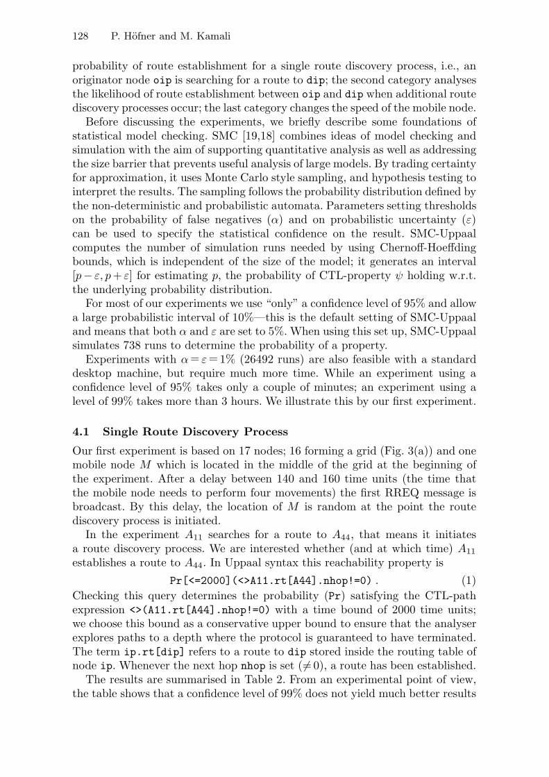
128 P. Hofner and M. Kamali
probability of route establishment for a single route discovery process, i.e., anoriginator node oip is searching for a route to dip; the second category analysesthe likelihood of route establishment between oip and dip when additional routediscovery processes occur; the last category changes the speed of the mobile node.
Before discussing the experiments, we briefly describe some foundations ofstatistical model checking. SMC [19,18] combines ideas of model checking andsimulation with the aim of supporting quantitative analysis as well as addressingthe size barrier that prevents useful analysis of large models. By trading certaintyfor approximation, it uses Monte Carlo style sampling, and hypothesis testing tointerpret the results. The sampling follows the probability distribution defined bythe non-deterministic and probabilistic automata. Parameters setting thresholdson the probability of false negatives (α) and on probabilistic uncertainty (ε)can be used to specify the statistical confidence on the result. SMC-Uppaalcomputes the number of simulation runs needed by using Chernoff-Hoeffdingbounds, which is independent of the size of the model; it generates an interval[p− ε, p+ ε] for estimating p, the probability of CTL-property ψ holding w.r.t.the underlying probability distribution.
For most of our experiments we use “only” a confidence level of 95% and allowa large probabilistic interval of 10%—this is the default setting of SMC-Uppaaland means that both α and ε are set to 5%. When using this set up, SMC-Uppaalsimulates 738 runs to determine the probability of a property.
Experiments with α= ε=1% (26492 runs) are also feasible with a standarddesktop machine, but require much more time. While an experiment using aconfidence level of 95% takes only a couple of minutes; an experiment using alevel of 99% takes more than 3 hours. We illustrate this by our first experiment.
4.1 Single Route Discovery Process
Our first experiment is based on 17 nodes; 16 forming a grid (Fig. 3(a)) and onemobile node M which is located in the middle of the grid at the beginning ofthe experiment. After a delay between 140 and 160 time units (the time thatthe mobile node needs to perform four movements) the first RREQ message isbroadcast. By this delay, the location of M is random at the point the routediscovery process is initiated.
In the experiment A11 searches for a route to A44, that means it initiatesa route discovery process. We are interested whether (and at which time) A11
establishes a route to A44. In Uppaal syntax this reachability property is
Pr[<=2000](<>A11.rt[A44].nhop!=0) . (1)Checking this query determines the probability (Pr) satisfying the CTL-pathexpression <>(A11.rt[A44].nhop!=0) with a time bound of 2000 time units;we choose this bound as a conservative upper bound to ensure that the analyserexplores paths to a depth where the protocol is guaranteed to have terminated.The term ip.rt[dip] refers to a route to dip stored inside the routing table ofnode ip. Whenever the next hop nhop is set (�=0), a route has been established.
The results are summarised in Table 2. From an experimental point of view,the table shows that a confidence level of 99% does not yield much better results
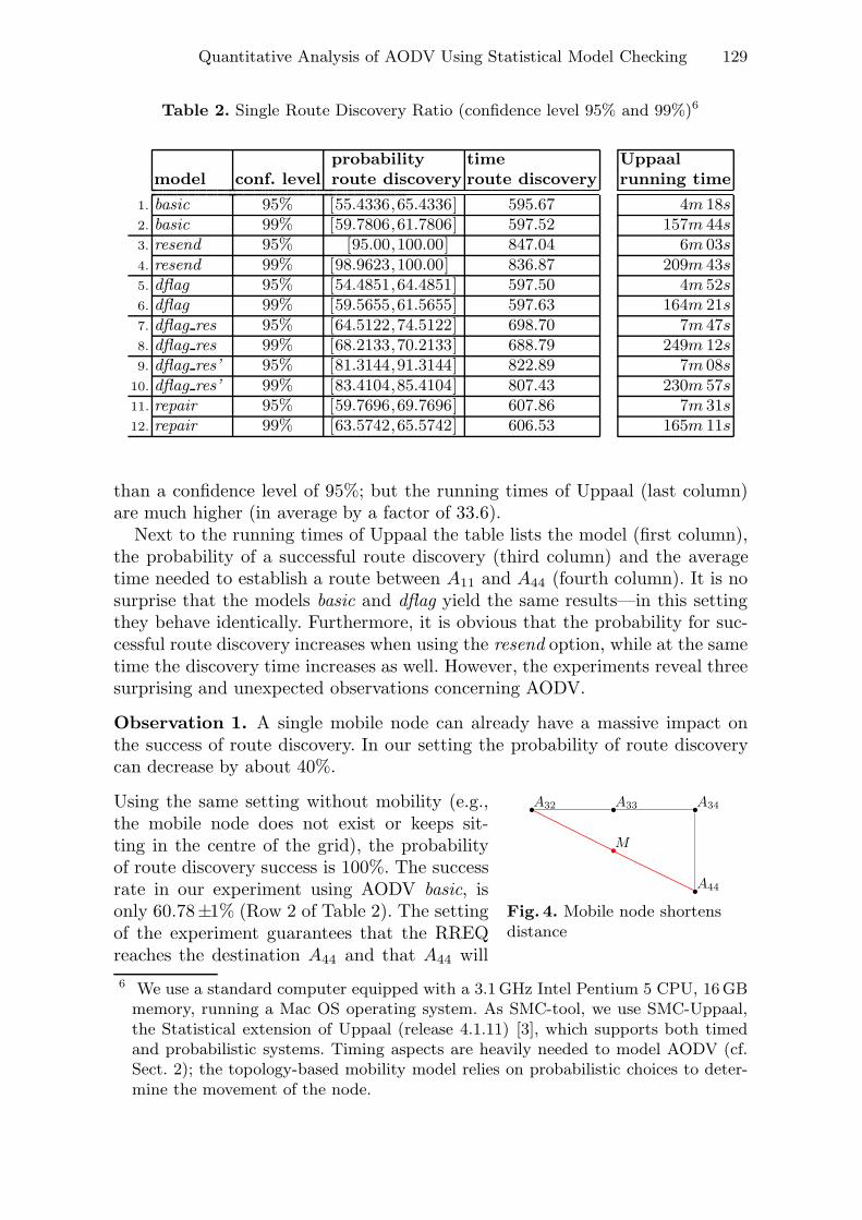
Quantitative Analysis of AODV Using Statistical Model Checking 129
Table 2. Single Route Discovery Ratio (confidence level 95% and 99%)6
probability time Uppaalmodel conf. level route discovery route discovery running time
1. basic 95% [55.4336,65.4336] 595.67 4m 18s2. basic 99% [59.7806,61.7806] 597.52 157m 44s3. resend 95% [95.00,100.00] 847.04 6m 03s4. resend 99% [98.9623,100.00] 836.87 209m 43s5. dflag 95% [54.4851,64.4851] 597.50 4m 52s6. dflag 99% [59.5655,61.5655] 597.63 164m 21s7. dflag res 95% [64.5122,74.5122] 698.70 7m 47s8. dflag res 99% [68.2133,70.2133] 688.79 249m 12s9. dflag res’ 95% [81.3144,91.3144] 822.89 7m 08s
10. dflag res’ 99% [83.4104,85.4104] 807.43 230m 57s11. repair 95% [59.7696,69.7696] 607.86 7m 31s12. repair 99% [63.5742,65.5742] 606.53 165m 11s
than a confidence level of 95%; but the running times of Uppaal (last column)are much higher (in average by a factor of 33.6).
Next to the running times of Uppaal the table lists the model (first column),the probability of a successful route discovery (third column) and the averagetime needed to establish a route between A11 and A44 (fourth column). It is nosurprise that the models basic and dflag yield the same results—in this settingthey behave identically. Furthermore, it is obvious that the probability for suc-cessful route discovery increases when using the resend option, while at the sametime the discovery time increases as well. However, the experiments reveal threesurprising and unexpected observations concerning AODV.
Observation 1. A single mobile node can already have a massive impact onthe success of route discovery. In our setting the probability of route discoverycan decrease by about 40%.
A32 A33 A34
A44
M
Fig. 4. Mobile node shortensdistance
Using the same setting without mobility (e.g.,the mobile node does not exist or keeps sit-ting in the centre of the grid), the probabilityof route discovery success is 100%. The successrate in our experiment using AODV basic, isonly 60.78±1% (Row 2 of Table 2). The settingof the experiment guarantees that the RREQreaches the destination A44 and that A44 will6 We use a standard computer equipped with a 3.1 GHz Intel Pentium 5 CPU, 16GB
memory, running a Mac OS operating system. As SMC-tool, we use SMC-Uppaal,the Statistical extension of Uppaal (release 4.1.11) [3], which supports both timedand probabilistic systems. Timing aspects are heavily needed to model AODV (cf.Sect. 2); the topology-based mobility model relies on probabilistic choices to deter-mine the movement of the node.
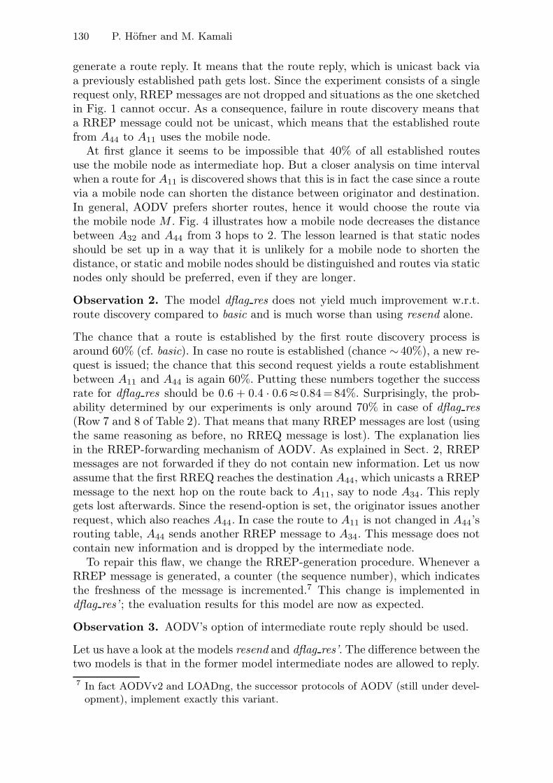
130 P. Hofner and M. Kamali
generate a route reply. It means that the route reply, which is unicast back viaa previously established path gets lost. Since the experiment consists of a singlerequest only, RREP messages are not dropped and situations as the one sketchedin Fig. 1 cannot occur. As a consequence, failure in route discovery means thata RREP message could not be unicast, which means that the established routefrom A44 to A11 uses the mobile node.
At first glance it seems to be impossible that 40% of all established routesuse the mobile node as intermediate hop. But a closer analysis on time intervalwhen a route for A11 is discovered shows that this is in fact the case since a routevia a mobile node can shorten the distance between originator and destination.In general, AODV prefers shorter routes, hence it would choose the route viathe mobile node M . Fig. 4 illustrates how a mobile node decreases the distancebetween A32 and A44 from 3 hops to 2. The lesson learned is that static nodesshould be set up in a way that it is unlikely for a mobile node to shorten thedistance, or static and mobile nodes should be distinguished and routes via staticnodes only should be preferred, even if they are longer.
Observation 2. The model dflag res does not yield much improvement w.r.t.route discovery compared to basic and is much worse than using resend alone.
The chance that a route is established by the first route discovery process isaround 60% (cf. basic). In case no route is established (chance ∼ 40%), a new re-quest is issued; the chance that this second request yields a route establishmentbetween A11 and A44 is again 60%. Putting these numbers together the successrate for dflag res should be 0.6 + 0.4 · 0.6≈ 0.84 =84%. Surprisingly, the prob-ability determined by our experiments is only around 70% in case of dflag res(Row 7 and 8 of Table 2). That means that many RREP messages are lost (usingthe same reasoning as before, no RREQ message is lost). The explanation liesin the RREP-forwarding mechanism of AODV. As explained in Sect. 2, RREPmessages are not forwarded if they do not contain new information. Let us nowassume that the first RREQ reaches the destination A44, which unicasts a RREPmessage to the next hop on the route back to A11, say to node A34. This replygets lost afterwards. Since the resend-option is set, the originator issues anotherrequest, which also reaches A44. In case the route to A11 is not changed in A44’srouting table, A44 sends another RREP message to A34. This message does notcontain new information and is dropped by the intermediate node.
To repair this flaw, we change the RREP-generation procedure. Whenever aRREP message is generated, a counter (the sequence number), which indicatesthe freshness of the message is incremented.7 This change is implemented indflag res’ ; the evaluation results for this model are now as expected.
Observation 3. AODV’s option of intermediate route reply should be used.
Let us have a look at the models resend and dflag res’. The difference between thetwo models is that in the former model intermediate nodes are allowed to reply.7 In fact AODVv2 and LOADng, the successor protocols of AODV (still under devel-
opment), implement exactly this variant.

Quantitative Analysis of AODV Using Statistical Model Checking 131
Looking at the results, we notice a dramatic difference in the likelihood of routediscovery. In the model resend the second request is followed by the generationof more than one RREP message. In fact, each node that established a route toA44 during the first RREQ-RREP-cycle (before the reply was lost), will generatea RREP message. Due to this, route establishment is guaranteed. In contrast,there is only one RREP message for each and every request in dflag res’. Thisobservation clearly indicates that intermediate route reply is a useful feature.Interestingly, there seems to be the tendency of preferring protocols withoutthis feature: the two successors of AODV, AODVv2 [16] and LOADng [6] followthis philosophy and set the D-flag as default—if at all, they allow intermediateroute reply as an optional feature.
Other Originator Nodes ● ●
●
●
●
●
1 2 3 4 5 650
60
70
80
90
100
distance between originator and destination
route
esta
blis
hm
ent (%
)
● classic/dflagresenddflag_resdflag_res'repair
Fig. 5. Probability of route-establishment
The first set of experiments con-sidered a route discovery fromA11 to A44, the largest distancea packet can travel in our setup. We expected to see the clear-est results by using this distance.However, we also performed ex-periments with all other pairs ofnodes. Fig. 5 summarises someresults. It illustrates the proba-bility of route-discovery (y-axis)depending on the distance be-tween originator and destination(x-axis). Of course, the largerthe distance between originatorand destination, the smaller thechance of route establishment. Interestingly, there is a clear drop down at a dis-tance of four nodes. It seems that from this point on resending guarantees thesuccess. Moreover, the graph illustrates that exhaustive MC cannot help: MC isusually limited to topologies of up to 6 nodes, distances of 5 hops and more arenot possible if one considers a non-linear topology.
4.2 Two Independent Route Discovery Processes
In order to evaluate the performance of variants of AODV under different net-work (traffic) load, we check the probability of route discovery when two routediscovery processes are performed in parallel. For this second set of experiments,we are again interested in a route from A11 to A44. However, shortly (35-45 mil-liseconds) after the packet is handed over to A11, a second data packet is injectedat another node, destined for some destination; in fact we did experiments forall destinations, but present only two observations—due to lack of space.
Observation 4. RREP messages are dropped more often than expected.

132 P. Hofner and M. Kamali
Table 3. Two route discovery processes looking for the same destination A44
distance orginator class probabilitybetween orig. of 2nd request (avg.)
1 {A12, A21} nodes at border 43.36%
2 {A13, A31} nodes at border 17, 75%{A22} inner node 13.28%
3 {A14, A41} nodes at border 43, 10%{A23, A32} inner nodes 29.74%
4 {A24, A42} nodes at border 71, 61%{A33} inner node 47.29%
5 {A34, A43} nodes at border 80.42%
We consider the scenario where the second request is sent from A22 to A44.Since some nodes drop RREP messages (cf. Sect. 2.2), the probability of routeestablishment between A11 and A44 should decrease (compared to the 60% ofTable 2). However, SMC-Uppaal shows that the probability of A11 finding a routeto A44 is in the probability interval [8.27913, 18.2791], i.e., a route discovery isunlikely. More results for the basic model are summarised in Table 3, groupedby the distance between the two originators. The table lists only the originatorof the second route request; both the originator (A11) of the first request andthe destination (A44) of both requests are fixed.
There is a correspondence between the success of route discovery and thedistance between the two originators; moreover inner nodes have more influenceon route discovery than nodes lying on the border of the network. This shows thatthe example of Fig. 1 occurs regularly. However, if the second originator oip2 isfar away from the first originator A11 no RREP message is dropped, since a routebetween oip2 and A44 is established before the RREQ from A11 reaches oip2. Inthe case of oip2 ∈ {A24, A42, A34, A43}, the probability even increases. This is inline with Observation 3: when intermediate route reply is enabled, more RREPmessage are generated and the probability of route discovery success grows.
Observation 5. “Busy” mobile nodes increase the chance of route discovery.
One could rephrase this observation to “adding noise sometimes increases per-formance”. At first glance it seems that adding additional network traffic—herea second route discovery processes—should not increase performance. But, letus look the scenario where the first data packet needs to be send from A11 toA44 (as before); the second packet is sent from A31 to the mobile node M . Whilehandling the second RREQ most of the nodes will not learn about A44 and A11.However it turns out that in the basic model, the probability of route discoveryincreases from around 60% to 72%. One reason is that the mobile node handlesthe request and generates a RREP message. While doing this it cannot handlethe first RREQ; in case the first RREQ is sent to M and it is handling a differentmessages (is busy), the message is buffered. If the message is buffered for a while,the chance that the RREQ from A11 reaches A44 via a path without M as an

Quantitative Analysis of AODV Using Statistical Model Checking 133
Table 4. different mobile node speed and impact on AODV variants
model probabilityfast probabilitymoderate probabilityslow
basic [48.5230,58.5230] [55.4336,65.4336] [61.9377,71.9377]
resend [94.8645,100.00] [95.00,100.00] [94.3225,100.00]
dflag [50.0136,60.0136] [54.4851,64.4851] [63.2927,73.2927]
dflag res [60.1762,70.1762] [64.5122,74.5122] [70.6098,80.6098]
dflag res’ [75.8943,85.8943] [81.3144,91.3144] [85.5149,95.5149]
repair [54.0786,64.0786] [57.6016,67.6016] [65.5962,75.5962]
intermediate hop, increases. Hence not the shortest, but the “fastest” route isestablished from A44 to A11; this route is then used to send the RREP, since itdoes not use the mobile node as intermediate hop, the RREP is not lost.
4.3 Influence of Speed of Mobile Nodes
In our experiments the topology changes within a time frame of 35 to 45 mil-liseconds; This also determines the speed of the mobile node. One might arguethat the speed of the mobile node affects our analysis and that other speedscould yield different behaviour. As shown in Table 4, this is not the case—theprobabilities slightly change, but stay in the same ball park. Moreover the re-lationship between the different variants stays the same; a variant that is morereliable with a fast mobile node, is also more reliable with a slower node. Forthis category of experiments we enforce a topology change within the interval[25, 35] (fast), [35, 45] (moderate), and [95, 105] (slow), respectively.
5 Related Work
Model checking has been used to analyse routing protocols in general and AODVin particular. For example, Bhargavan et al. [1] were amongst the first to usemodel checking—they used the SPIN model checker—on a draft of AODV,demonstrating the feasibility and value of automated verification of routing pro-tocols. Musuvathi et al. [14] introduced the CMC model checker primarily tosearch for coding errors in implementations of protocols written in C. They usedAODV as an example and, as well as discovering a number of errors, they alsofound a problem with the specification itself, which has since been corrected.Chiyangwa and Kwiatkowska [4] used the timing features of UPPAAL to studythe relationship between the timing parameters and the performance of routediscovery. None of these studies performed a quantitative analysis of AODV.
Statistical model checking techniques [19,18] are rather new. So far they havebeen used in a couple of case studies. Bulychey et al. [2] for example applythe SMC-Uppaal to an analysis of an instance of the Lightweight Media access

134 P. Hofner and M. Kamali
Control (LMAC) protocol; by this they are able to analyse ring topologies ofup to 10 nodes.8 Applications of SMC within biological systems are discussedin [5,13]. To the best of our knowledge, SMC was not used for the analysis ofrouting protocols so far—except in [11], where SMC-Uppaal is used to compareAODV and DYMO and to illustrate that even large topologies (up to 100 nodes)can be analysed by SMC. Our experiments are in line with this. However, it isunique in the sense that we carefully study variants of AODV.
6 Conclusion and Future Work
The aim of this paper has been a careful (quantitative) analysis of AODV andits variants using statistical model checking techniques. By this, we have madesurprising observations on the behaviour of AODV. We have shown for exam-ple that some optional features (D-flag) should not be combined with others(resending). Another result shows that a well-known shortcoming occurs moreoften than expected and has a tremendous effect on the success of route estab-lishment. One challenge we faced while performing our experiments has been theinterpreting the data.
The results were often surprising and hard to interpret, particularly whenthey indicate odd behaviour. Unfortunately SMC-Uppaal does not store tracesduring analysis, thus it is difficult to recover counterexamples to explain theobservations. At the moment counter examples are constructed “by hand” byformulating more probing queries beyond looking at overall performance. Thissuggests that more powerful statistical analysis such as “rare event simulation”in combination with multiple queries could be used to compile better evidence.
Next to this careful analysis, we also showed that SMC is a suitable tool foranalysing WMNs. In this setting classical MC was limited to topologies with upto 6 nodes and therefore having a realistic mobility model was not possible.
Future work will be a continuation of our case study. In particular we wantto look at topologies of up to 100 nodes—it has been shown that an analysisof such networks is possible [11]. However, choosing the right scenario is crucialhere: Since one cannot analyse all scenarios, one has to pick the right topologiesand the right mobility model(s); but in some sense finding the correct settingbecomes a “stab in the dark”. We hope that our previous experience helps toset the experiments right.
Acknowledgement. We thank Ansgar Fehnker, Rob van Glabbeek and FranckCassez for fruitful discussions and their help.
NICTA is funded by the Australian Government as represented by the De-partment of Broadband, Communications and the Digital Economy and theAustralian Research Council through the ICT Centre of Excellence program.
8 Other case studies include firewire, bluetooth, and a train gate(see http://people.cs.aau.dk/~adavid/smc/cases.html for an overview).
Quantitative Analysis of AODV Using Statistical Model Checking 135
References
1. Bhargavan, K., Obradovic, D., Gunter, C.A.: Formal verification of standards fordistance vector routing protocols. J. ACM 49(4), 538–576 (2002)
2. Bulychev, P., David, A., Guldstrand Larsen, K., Legay, A., Mikucionis, M., BøgstedPoulsen, D.: Checking and distributing statistical model checking. In: Goodloe,A.E., Person, S. (eds.) NFM 2012. LNCS, vol. 7226, pp. 449–463. Springer, Hei-delberg (2012)
3. Bulychev, P., David, A., Larsen, K., Mikucionis, M., Bøgsted Poulson, D., Legay,A., Wang, Z.: UPPAAL-SMC: Statistical model checking for priced timed au-tomata. In: Wiklicky, H., Massink, M. (eds.) Quantitative Aspects of ProgrammingLanguages. EPTCS, vol. 85, pp. 1–16. Open Publishing Association (2012)
4. Chiyangwa, S., Kwiatkowska, M.: A timing analysis of AODV. In: Steffen, M.,Zavattaro, G. (eds.) FMOODS 2005. LNCS, vol. 3535, pp. 306–321. Springer, Hei-delberg (2005)
5. Clarke, E.M., Faeder, J.R., Langmead, C.J., Harris, L.A., Jha, S.K., Legay, A.:Statistical Model Checking in BioLab: Applications to the automated analysis ofT-cell receptor signaling pathway. In: Heiner, M., Uhrmacher, A.M. (eds.) CMSB2008. LNCS (LNBI), vol. 5307, pp. 231–250. Springer, Heidelberg (2008)
6. Clausen, T., Colin de Verdiere, A., Yi, J., Niktash, A., Igarashi, Y., Satoh, H., Her-berg, U., Lavenu, C., Lys, T., Perkins, C., Dean, J.: The lightweight on-demand adhoc distance-vector routing protocol - next generation (LOADng). Internet Draft(Standards Track) (2013),http://tools.ietf.org/html/draft-clausen-lln-loadng-08
7. Fehnker, A., van Glabbeek, R., Hofner, P., McIver, A., Portmann, M., Tan, W.L.:Automated analysis of AODV using UPPAAL. In: Flanagan, C., Konig, B. (eds.)TACAS 2012. LNCS, vol. 7214, pp. 173–187. Springer, Heidelberg (2012)
8. Fehnker, A., van Glabbeek, R.J., Hofner, P., McIver, A., Portmann, M., Tan, W.L.:A process algebra for wireless mesh networks used for modelling, verifying andanalysing AODV. Tech. Rep. 5513, NICTA (2013),http://www.nicta.com.au/pub?id=5513
9. Fehnker, A., Hofner, P., Kamali, M., Mehta, V.: Topology-based mobility modelsfor wireless networks. In: Joshi, K., Siegle, M., Stoelinga, M., D’Argenio, P.R. (eds.)QEST 2013. LNCS, vol. 8054, pp. 389–404. Springer, Heidelberg (2013)
10. Hofner, P., van Glabbeek, R., Tan, W., Portmann, M., McIver, A., Fehnker, A.: Arigorous analysis of AODV and its variants. In: Modeling, Analysis and Simulationof Wireless and Mobile Systems, MSWIM 2012, pp. 203–212. ACM (2012)
11. Hofner, P., McIver, A.: Statistical model checking of wireless mesh routing proto-cols. In: Brat, G., Rungta, N., Venet, A. (eds.) NFM 2013. LNCS, vol. 7871, pp.322–336. Springer, Heidelberg (2013)
12. IEEE P802.11s: IEEE draft standard for information technology—telecommunications and information exchange between systems—local andmetropolitan area networks—specific requirements—part 11: Wireless LANMedium Access Control (MAC) and physical layer (PHY) specifications-amendment 10: Mesh networking (July 2010)
13. Jha, S.K., Clarke, E.M., Langmead, C.J., Legay, A., Platzer, A., Zuliani, P.: Abayesian approach to model checking biological systems. In: Degano, P., Gorrieri,R. (eds.) CMSB 2009. LNCS, vol. 5688, pp. 218–234. Springer, Heidelberg (2009)
14. Musuvathi, M., Park, D.Y.W., Chou, A., Engler, D.R., Dill, D.L.: CMC: a prag-matic approach to model checking real code. In: Operating Systems Design andImplementation, OSDI 2002 (2002)

136 P. Hofner and M. Kamali
15. Perkins, C., Belding-Royer, E., Das, S.: Ad hoc on-demand distance vector (AODV)routing. RFC 3561 (Experimental) (2003), http://www.ietf.org/rfc/rfc3561
16. Perkins, C., Chakeres, I.: Dynamic MANET on-demand (AODVv2) routing. Inter-net Draft (Standards Track) (2013),http://tools.ietf.org/html/draft-ietf-manet-dymo-25
17. Perkins, C., Royer, E.: Ad-hoc On-Demand Distance Vector Routing. In: 2nd IEEEWorkshop on Mobile Computing Systems and Applications, pp. 90–100 (1999)
18. Sen, K., Viswanathan, M., Agha, G.A.: Vesta: A statistical model-checker andanalyzer for probabilistic systems. In: Quantitative Evaluaiton of Systems, QEST2005, pp. 251–252. IEEE (2005)
19. Younes, H.: Verification and Planning for Stochastic Processes with AsynchronousEvents. Ph.D. thesis, Carnegie Mellon University (2004)

Paper V
Re�nement-Based Modeling of 3D NoCs
Maryam Kamali, Luigia Petre, Kaisa Sere
and Masoud Daneshtalab
Originally published in: F. Arbab and M. Sirjani (Eds.), Proceedings of the4th IPM International Conference on Fundamentals of Software Engineering- FSEN 11, Lecture Notes in Computer Science Vol. 7141, pp. 236-252,Springer-Verlag, 2012.
137

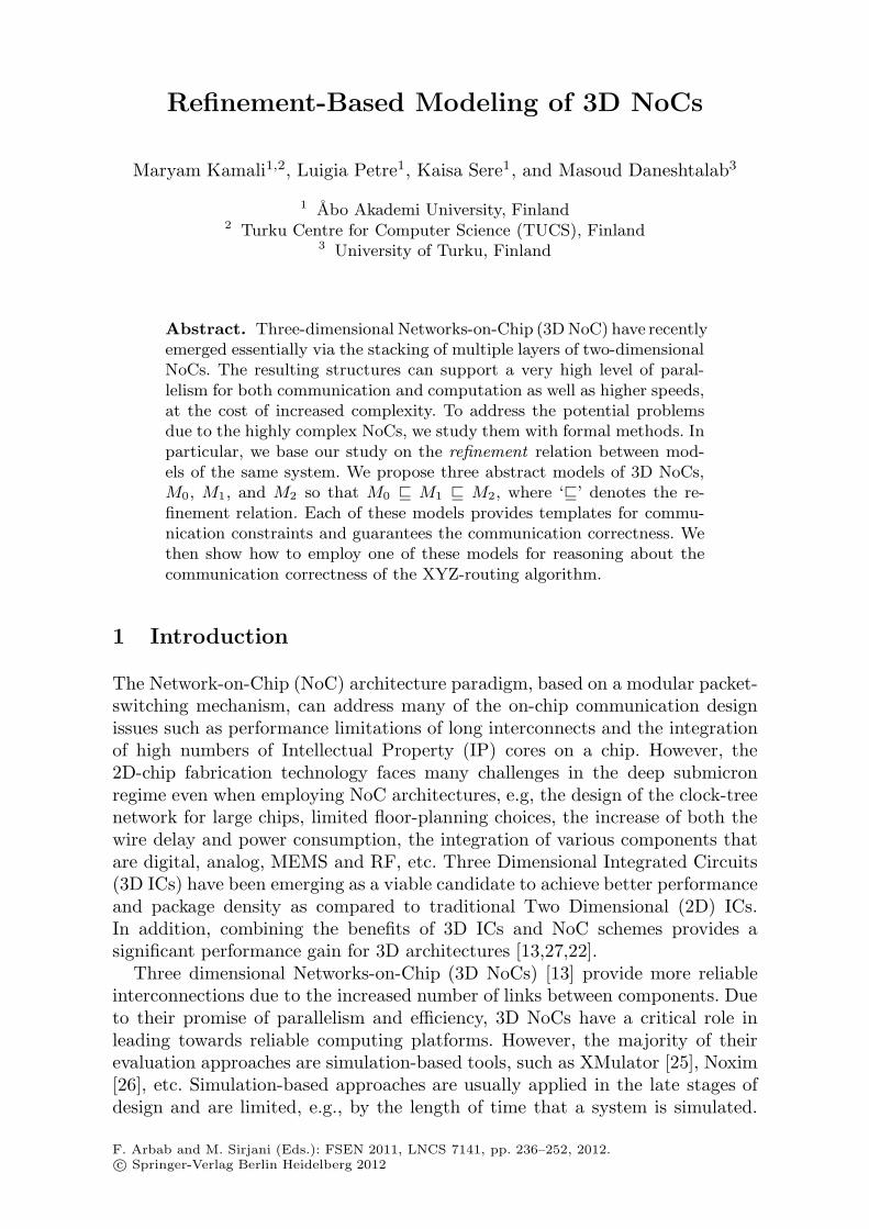
Refinement-Based Modeling of 3D NoCs
Maryam Kamali1,2, Luigia Petre1, Kaisa Sere1, and Masoud Daneshtalab3
1 Abo Akademi University, Finland2 Turku Centre for Computer Science (TUCS), Finland
3 University of Turku, Finland
Abstract. Three-dimensional Networks-on-Chip (3D NoC) have recentlyemerged essentially via the stacking of multiple layers of two-dimensionalNoCs. The resulting structures can support a very high level of paral-lelism for both communication and computation as well as higher speeds,at the cost of increased complexity. To address the potential problemsdue to the highly complex NoCs, we study them with formal methods. Inparticular, we base our study on the refinement relation between mod-els of the same system. We propose three abstract models of 3D NoCs,M0, M1, and M2 so that M0 � M1 � M2, where ‘�’ denotes the re-finement relation. Each of these models provides templates for commu-nication constraints and guarantees the communication correctness. Wethen show how to employ one of these models for reasoning about thecommunication correctness of the XYZ-routing algorithm.
1 Introduction
The Network-on-Chip (NoC) architecture paradigm, based on a modular packet-switching mechanism, can address many of the on-chip communication designissues such as performance limitations of long interconnects and the integrationof high numbers of Intellectual Property (IP) cores on a chip. However, the2D-chip fabrication technology faces many challenges in the deep submicronregime even when employing NoC architectures, e.g, the design of the clock-treenetwork for large chips, limited floor-planning choices, the increase of both thewire delay and power consumption, the integration of various components thatare digital, analog, MEMS and RF, etc. Three Dimensional Integrated Circuits(3D ICs) have been emerging as a viable candidate to achieve better performanceand package density as compared to traditional Two Dimensional (2D) ICs.In addition, combining the benefits of 3D ICs and NoC schemes provides asignificant performance gain for 3D architectures [13,27,22].
Three dimensional Networks-on-Chip (3D NoCs) [13] provide more reliableinterconnections due to the increased number of links between components. Dueto their promise of parallelism and efficiency, 3D NoCs have a critical role inleading towards reliable computing platforms. However, the majority of theirevaluation approaches are simulation-based tools, such as XMulator [25], Noxim[26], etc. Simulation-based approaches are usually applied in the late stages ofdesign and are limited, e.g., by the length of time that a system is simulated.
F. Arbab and M. Sirjani (Eds.): FSEN 2011, LNCS 7141, pp. 236–252, 2012.c© Springer-Verlag Berlin Heidelberg 2012

Refinement-Based Modeling of 3D NoCs 237
This means that exhaustive checking of all the system states is impossible inpractice for complex 3D NoCs and thus, simulation is not suitable for verifyingthe correctness of a NoC design.
Another approach to address this problem is via formal methods. Formalmethods refer to the application of mathematical techniques to the design andimplementation of computer hardware and software. Prominent examples of ap-plying formal methods are provided by, e.g., Intel [16,19] and IBM [21] forformally verifying hardware or systems-on-chip (SoC) [15]. By using rigorousmathematical techniques, it is possible to deliver provably correct systems. For-mal methods are based on the capture of system requirements in a specific, pre-cise format. Importantly, such a format can be analyzed for various propertiesand, if the formal method permits, also stepwise developed until an implemen-tation is formed. By following such a formal development, we are sure that thefinal result correctly implements the requirements of the system.
Much of the research concerning the 3D NoC design is concentrated on var-ious bottom-up approaches, such as the study of routing algorithms [6,20] orthe design of dedicated 3D NoC architectures [29] where parameters such ashop count or power consumption are improved. Here we are concerned with areverse, top-down approach where we start from simple models and add com-plexity later. There are already research results regarding the detection of faultsas well as debugging in the early stages of NoC design. A generic model for spec-ifying and verifying NoC systems is presented in [10] where the formal verifica-tion is addressed with the ACL2 theorem prover, a mechanized proof tool. Thistool produces a set of proof obligations that should be discharged for particularNoC instances. This generic model has been used for verification of functionalityfeatures in 2D-NoC systems. Another formal approach to the development ofthe NoC systems employing the B-action systems formalism has been describedin [28], where the focus is on the formal specification of communication routers. Aframework for modeling 2D-NoC systems by composing more advanced routingcomponents out of simpler ones, is proposed there.
In this paper, we go one step further and propose a top-down formalizationof the early 3D NoC design. The formal method we employ is Event-B [2] whichcomes with the associated tool Rodin [1,30]. One of the main features of Event-B is that the system development is done in a stepwise manner that eventuallyleads to a system implementation. The stepwise development is captured by therefinement [4,5] relation between models of the same system, so that a high-levelmodel of a system is transformed by a sequence of correctness-preserving stepsinto a more detailed and efficient model that satisfies the original specification.We specify here the general structure of a 3D NoC at a high level of abstraction inEvent-B. The specification formulates the main constraints of the communicationmodel, needed to prove its correctness. Our definition for correctness at thisabstract level of modeling is to show that a package injected in the networkis eventually received at the destination. We propose three different abstractmodels M0, M1, and M2 for a 3D NoC so that M0 � M1 � M2, where ‘�’denotes the refinement relation. Furthermore, each of these models can be refined

238 M. Kamali et al.
into more concrete models to define specific 3D NoC designs in the early stagesof the system development. When the concrete models preserve the correctnessproperties of the abstract models, we guarantee the correctness of the concrete3D NoC designs. As an application of the general 3D NoC designs, we model theXYZ routing algorithm by refining the M2 abstract model. To verify the XYZrouting algorithm, we generate the proof obligations using the Rodin tool anddischarge them automatically or interactively.
We proceed as follows. In Section 2 we overview the Event-B formal methodto the extent needed in this paper. In Section 3 we propose three increasinglymore detailed formal models for a 3D NoC together with the constraints forproving correctness. In Section 4 we illustrate the formal modeling of the XYZrouting algorithm as a case study. In Section 5 we discuss the proof obligationswhile in Section 6 we present concluding remarks and future work.
2 Preliminaries
Event-B [2,1] is an extension of the B formalism [3,28] for specifying distributedand reactive systems. A system model is gradually specified on increasing levelsof abstraction, always ensuring that a more concrete model is a correct imple-mentation of an abstract model. The language and proof theory of Event-Bare based on logic and set theory. The correctness of the stepwise constructionof formal models is ensured by discharging a set of proof obligations: if theseobligations hold, then the development is mathematically shown to be correct.Event-B comes with the associated tool Rodin [1,30], which automatically dis-charges part of the proof obligations and also provides the means for the user todischarge interactively the remaining proofs.
Each Event-B model consists of two components called context and machine.A context describes the static part of the model, i.e., it introduces new typesand constants. The properties of these types and constants are gathered as a listof axioms. A machine represents the dynamic part of the model, consisting ofvariables that define the state of the model and operations called events. Thesystem properties that should be preserved during the execution are formulatedas a list of invariant predicates over the state of the model.
An event, modeling state changes, is composed of a guard and an action. Theguard is the necessary condition under which an event might occur; if the guardholds, we call the event enabled. The action determines the way in which the statevariables change when the event occurs. For initializing the system, a sequenceof actions is defined. When the guards of several events hold at the same time,then only one event is non-deterministically chosen for execution. If some eventshave no variables in common and are enabled at the same time, then they canbe considered to be executed in parallel since their sequential execution in anyorder gives the same result. For all practical purposes, this execution model isparallel and can be implemented as such when the model is refined to code.Events can be declared as anticipated, meaning that in the future refinementswe need to set out a natural number expression called variant and prove that it

Refinement-Based Modeling of 3D NoCs 239
is decreased by this event. Events can also be convergent, meaning that in thecurrent machine there is a variant that decreases when this event is chosen forexecution. Thus, an anticipated event is not convergent in the current machinebut should become so in a future refinement of that machine.
A model can be developed by a number of correctness preserving steps calledrefinements [4,5]. One form of model refinement can add new data and newevents on top of the already existing data and behavior but in such a way thatthe introduced behavior does not contradict or take over the abstract machinebehavior. This form of stepwise construction is referred to as superposition re-finement [18,9]. We may also use other refinement forms, e.g., algorithmic refine-ment [8]. In this case, an event of an abstract machine can be refined by severalcorresponding events in a refined machine. This will model different branches ofexecution, that can, for instance, take place in parallel and thus can improve thealgorithmic efficiency. In this paper, we use only superposition refinement.
3 Three Abstract Models for the 3D NoC: M0, M1, M2
In this section we formally develop three high-level models M0, M1, and M2
for the 3D NoC. Our models are at three increasing levels of detail so thateach model is a refinement of the previous one: M0 � M1 � M2. In the initialmodel, we specify a network of nodes and define the correctness properties ofthis network based on a specific data structure called pool, as suggested by [2].In the second model, we add new data and events to model the 3D mesh-basedNoC architecture; besides, we specify the channels between nodes. In the thirdmodel, we model buffers for nodes and refine the communication model.
By starting from an initial model that is rather abstract, i.e., without detailingthe communication topology, we obtain a rather general starting point that canlater be refined to various topologies. Moreover, adding channels and ports onlyin the second model leads to a clean modelling of the basic communicationmechanism (via routing and switching) in the initial model; the required detail(of channels and ports) are not needed for understanding the communicationmechanism. Adding buffers in the third model illustrates an extra level of detail.Networks where the nodes have no buffers for communication will, therefore,employ the second model as their abstraction and not the third.
3.1 The Initial Model M0
The first model M0 that we construct is rather abstract: we do not considerthe numerous parts of the network such as channels or buffers; they will beintroduced in subsequent refinements. M0 will thus allow us to reason about thesystem very abstractly [2]. The model M0 is formed of the static part and thedynamic part, as follows.
The Static Part. The static part of our model is described in Fig. 1 andcontains the sets MESSAGES, ROUTER, DATA and the constants data, des,src and Neigh. The message identifiers are modeled by the non-empty and finite

240 M. Kamali et al.
MESSAGES set. We use the following modeling idea for messages. A message idin the MESSAGES set relates to a triple (data, source, destination) where datais an element of the DATA set, source models the source node where a messageis injected, and destination models the destination node where a message shouldbe received. A message should not be destined to its source node. The set ofnetwork nodes and data are modeled by the sets ROUTER (finite and non-empty) and DATA (finite and non-empty), respectively. The relation Neigh (non-empty, symmetric, and non-reflexive) models the neighbor structure i.e., whichnode can communicate with which node.
SETS MESSAGES ROUTER DATACONSTANTS data des src NeighAXIOMS
MESSAGES �= ∅ ∧ finite(MESSAGES)ROUTER �= ∅ ∧ finite(ROUTER)DATA �= ∅ ∧ finite(DATA)data ∈ MESSAGES →DATAsrc ∈ MESSAGES →ROUTER ∧ des ∈ MESSAGES → ROUTER∀m, sp, dp ·m ∈ MESSAGES ∧ sp ∈ ROUTER ∧ dp ∈ ROUTER
∧m �→ sp ∈ src ∧m �→ dp ∈ des ⇒ sp �= dpNeigh ∈ ROUTER↔ROUTERNeigh �= ∅ ∧ Neigh = Neigh−1 ∧ dom(Neigh) � id ∩ Neigh = ∅
Fig. 1. M0: the static part
To define structure types such as records in Event-B, we use functions torepresent attributes. Therefore, our modeling idea translates to the functionsdata, src and des with ranges DATA, ROUTER, and ROUTER, respectively.
The Dynamic Part. In our network model we use the following condition formodeling the communication correctness: the messages in the network will even-tually reach their destinations. For this, we define two message subsets and onepartial message-to-node map as machine variables: sent pool ⊆MESSAGES,received pool⊆MESSAGES and moving pool∈sent pool �→ROUTER.
The sent pool subset denotes the list of messages injected into the network.The sent pool subset is updated whenever a new message is injected into the net-work, while the moving pool subset denotes the current position of traveling mes-sages. All the messages injected into the network are added to the moving pooland whenever a message is routed from a node to another one, the current po-sition of that message is updated in the moving pool. The received pool subsetdenotes the list of messages received from the network by destination nodes.Whenever a message is received at its destination, it will be added to received pooland removed from moving pool. The behavior of message pools is illustrated inFig. 2.
To model the communication and the message pool functions, we define threeevents as explained below. The sent message event described in Fig. 3(a) han-dles the injection of a new message into the network. Whenever a message isinjected into the network both sent pool as well as moving pool are updated.

Refinement-Based Modeling of 3D NoCs 241
Fig. 2. Message Pools
Event sent message =anycurrent msg
wherecurrent msg ∈ MESSAGEScurrent msg /∈ sent pool
thensent pool :=sent pool∪{current msg}moving pool := moving pool∪{current msg �→src(current msg)}
end
(a) Message Injection
Event routing =beginskip
endEvent switching =Statusanticipated
anycurrent msg new position
wherecurrent msg ∈ dom(moving pool)des(current msg) �=moving pool(current msg)
new position �→moving pool(current msg)∈Neigh
new position �= src(current msg)thenmoving pool(current msg):=new position
end
(b) Routing and Switching
Fig. 3. M0 Events
A message in moving pool should be routed toward its destination. This iscomposed of two actions, one for deciding which node would be the next one(routing) and the other for transferring the message to that node (switching).These two actions are available for all the nodes, including the source, the des-tination as well as all the intermediate nodes and are modeled respectively bythe routing and switching events shown in Fig. 3(b). In this abstract model wedo not have any routing decisions, hence, the routing event is modeled by skip.The switching event in the M0 model only transfers a message from the currentnode to one of its neighbors nondeterministically and updates the moving poolby changing the current position of a message. To avoid cycling, we do not al-low a message to return to its source. The reason for not considering a specificrouting algorithm is that it makes our initial model more general and reusablefor a wide variety of routing algorithms implementations. The switching eventhas the status anticipated.
Event received message =Status convergent
anycurrent msg
wherecurrent msg ∈ dom(moving pool)des(current msg) = moving pool(current msg)
thenmoving pool := {current msg}�−moving poolreceived pool := received pool ∪ {current msg}
end
Fig. 4. M0: Received message Event

242 M. Kamali et al.
The received message event shown in Fig. 4 adds a message received at itsdestination to received pool and removes the message from moving pool. Thisevent is convergent: if new messages are not injected to the network for a certaintime, all the messages will be received at their destinations. This is proved bymeans of the (sent pool \ received pool) variant denoting the difference betweenthe sets sent pool and received pool.
In order to prove the communication correctness, we need to prove that thesent pool subset eventually becomes equal with the received pool subset andthe moving pool subset is empty when all the messages are received at theirdestinations. These properties are formulated in Fig. 5 as invariants.
INVARIANTSdom(moving pool) ⊆ sent poolreceived pool ∩ dom(moving pool) = ∅sent pool = received pool ⇔moving pool = ∅∀msg ·msg /∈ sent pool ⇒msg /∈ received poolsent pool \ dom(moving pool) = received poolsent pool \ received pool = dom(moving pool)
Fig. 5. M0: Invariants (Pool Modeling)
M0 is a general specification of a general network and will be refined to model3D NoC communication designs in the following. Moreover, the model providesthe necessary properties that should be preserved by refinement. These proper-ties, that guarantee the overall communication correctness, are defined as thelist of invariants.
3.2 The Second Model M1
Transferring a message from a node to its neighbor in the model M0 is achievedsimply by copying the message from a node to another. In this section we refinethe initial model M0 to also specify channels specific to the 3D NoCs. To specifychannels, we need a 3D NoC architecture. There are a number of 3D NoC archi-tectures, e.g., mesh-based [13], tree-based [14]. We consider here NoCs with 3Dmesh topologies. The 3D mesh-based NoC (Fig. 6(a)) consists of N = m ∗ n ∗ knodes; each node has an associated integer coordinate triple (x, y, z), 0 < x ≤ m,0 < y ≤ n, 0 < z ≤ k.
Fig. 6. (a) 3D Mesh-based NoC architecture (b) Router channels

Refinement-Based Modeling of 3D NoCs 243
Our 3D NoC architecture employs seven-port routers: one port to the IPblock, one port to above and below routers, and one in each cardinal direction(North, South, East and West), as shown in Fig. 6(b).
The Static Part. We extend the static part of the initial model M0 in threeways: we map routers to coordinate triples, we add new properties for the neighrelation based on the coordinate triples, and we model ports and channels forthe 3D NoC. In order to map routers to the coordinate triples, we define fourconstants: coordX , coordY , coordZ and mk position as shown in Fig. 7. ThecoordX , coordY and coordZ constants represent coordinate triples (x, y, z) andthe mk position constant is a map associating each router to a position in spacegiven by the coordinates. The crossbarX , crossbarY and crossbarZ constantsmodel the number of nodes in X, Y and Z coordinate in the network, respectively.
Two nodes with coordinates (xi, yi, zi) and (xj , yj , zj) are connected by acommunication channel if and only if |xi−xj |+ |yi−yj |+ |zi−zj| = 1. To modelthis neighbor structure, the Neigh relation in the initial model M0 is restrictedin this model by adding the axiom in Fig. 8.
SETS CHANNEL PORTSCONSTANTS coordX coordY coordZ mk position
crossbarX crossbarY crossbarZ mk channelAXIOMS
crossbarX ∈ N1 ∧ crossbarY ∈ N1 ∧ crossbarZ ∈ N1
mk position ∈ (1 .. crossbarX )× (1 .. crossbarY )× (1 .. crossbarZ ) �� ROUTERcoordX ∈ ROUTER � (1 .. crossbarX )coordY ∈ ROUTER � (1 .. crossbarY )coordZ ∈ ROUTER � (1 .. crossbarZ )∀xx , yy, zz ·xx ∈ 1 .. crossbarX ∧ yy ∈ 1 .. crossbarY ∧ zz ∈ 1 .. crossbarZ
⇒coordX (mk position(xx �→ yy �→ zz)) = xx∧coordY (mk position(xx �→ yy �→ zz)) = yy∧coordZ (mk position(xx �→ yy �→ zz)) = zz
∀pos1 ,pos2 ·pos1 ∈ ROUTER ∧ pos2 ∈ ROUTER ∧ pos1 �= pos2⇒coordX (pos1 ) �= coordX (pos2 )∨ coordY (pos1 ) �= coordY (pos2 )∨
coordZ (pos1 ) �= coordZ (pos2 )
Fig. 7. M1: Static Part 1
We define the CHANNEL set to model the communication channels betweenrouters and we define the PORTS set to define the input and output ports of nodesin the static part of the second model. To show how two neighbors are connectedto each other through channels, we define the def channel and mk channel rela-tions with the help of axioms, as shown in Fig. 8. The def channel relation modelsthe relation of a port of a node to the corresponding port of its neighbor and themk channel relation maps the port relations to channels.
AXIOMS∀r1 , r2 ·r1 �→ r2 ∈ Neigh ⇔ abs(coordX (r1 )− coordX (r2 )) + abs(coordY (r1 )
−coordY (r2 )) + abs(coordZ (r1 )− coordZ (r2 )) = 1def channel ∈ (ROUTER × PORTS)→ (ROUTER × PORTS)partition(PORTS , {Ein}, {Eout}, {Win}, {Wout}, {Nin}, {Nout}, {Sin}
, {Sout}, {Uin}, {Uout}, {Din}, {Dout}, {Lin}, {Lout})mk channel ∈ def channel �� CHANNELS
Fig. 8. M1: Static Part 2

244 M. Kamali et al.
East and west ports of neighbor nodes with different X coordinate are relatedto each other through a channel. For instance, as shown in Fig. 9, Ein and Eoutports of node (1, 1, 1) are connected to Wout and Win ports of node (2, 1, 1)through a channel ((1, 1, 1) �→ Eout) �→ ((2, 1, 1) �→ Win) and ((2, 1, 1) �→Wout) �→ ((1, 1, 1) �→ Ein) relations in def channel. This connection of theports of the neighboring nodes on the X coordinate is modeled by the axiomshown in Fig. 10. The port relation between neighbors on other coordinates isdefined by similar axioms which are not shown here due to lack of space.
Fig. 9. Channels in 3D Mesh-Based NoCs
The Dynamic Part. In the static part of the model M1, we define the 3Dmesh NoC architecture with the triple coordinate of nodes and their channels.In the dynamic part of the model M1, we refine the dynamic part of the modelM0 to specify the transferring of data through the communication channels, sothat the overall correctness of communication holds.
The communication channels between routers are considered asynchronouschannels, transferring data upon request. Each channel propagates data as wellas control values. In our case, a control value models the fact that a channel isoccupied by a message. When a message is injected to a channel, the controlvalue of that channel is set to busy and when the message is received at theother side of channel, the control value of that channel is set to free.
AXIOMS∀n, m, i, j ·(n �→ i) �→ (m �→ j) ∈ def channel ∧ i = Wout ∧ j = Ein⇔coordX (n)− coordX (m) = 1 ∧ coordY (n) = coordY (m) ∧ coordZ (n) = coordZ (m)∀n, m, i, j ·(n �→ i) �→ (m �→ j) ∈ def channel ∧ i = Eout ∧ j = Win⇔coordX (n)− coordX (m) = −1 ∧ coordY (n) = coordY (m) ∧ coordZ (n) = coordZ (m)
Fig. 10. M1: Static Part 3
In order to model the transferring of messages through the communicationchannels, the variables channel state and channel content are defined in thesecond model to represent the control and the data value on each channel. Eachchannel can have the busy or free state. When the channel receives data, its stateswitches from free to busy and the message is added to the channel content.When the channel transfers data to the end, channel state changes to freeand the channel is released by removing the message from channel content. Theinvariants of M1 model that, when a channel is released, then its content is emptyand can thus receive the next message; when a channel is busy, the message isin the channel. We illustrate these invariants in Fig.11.

Refinement-Based Modeling of 3D NoCs 245
VARIABLESchannel content channel state
INVARIANTSchannel content ∈ CHANNELS �� MESSAGESdom(channel content) = channel state−1 [{busy}]channel state ∈ CHANNELS → statedom(channel state) = ran(mk channel)ran(channel content) ⊆ dom(moving pool)∀msg ·msg ∈ dom(moving pool) ∧ des(msg) = moving pool(msg)
⇒msg /∈ ran(channel content)
Fig. 11. M1: Invariants (channels)
The switching event is now refined to transfer a message to the next routerthrough channels. In order to model this, we add a new event out to channel asshown in Fig.15 (Appendix) to model pushing a message in the channel. Thisevent is enabled when there is a message for transferring in a node and thechannel between the node and the next node is free. In addition, we refine theswitching event as shown in Fig.16 (Appendix) to model releasing the channelby receiving the message at the end of the channel. This event is enabled whena message is in the channel.
3.3 The Third Model M2
In this model, we define buffers for the ports of the nodes and refine the secondmodel to model the communication in 3D NoCs by considering these buffers.
The Static Part. The context of the third model contains a single constantbuffer size ∈ N1, which is a strict natural number denoting the maximumnumber of messages allowed in a buffer.
The Dynamic Part. Each node has fourteen buffers, each assigned to nodeports; those assigned to output ports are called output buffers and those assignedto input ports are called input buffers. When there is a message in an outputbuffer of a node, the node can transfer it to the channel provided that the channelis free. If in the other side of the channel the input buffer has an empty place,the message is transferred to the input buffer of the next node and the channelis released; otherwise, the channel will be busy until an empty place appearsin the input buffer. To model the buffer structure in the third model we adda new machine variable buffer content that models the current content of allbuffers. Indeed, adding and removing messages in/from buffers is modeled bythe buffer content variable.
In order to guarantee the correctness of the buffer modeling, we need theinvariants shown Fig.12. They model that the content of a buffer never becomesmore than its size. In addition, while a message is in the moving pool, i.e., ithas not reached to its destination, it must be either in a channel or in a buffer.
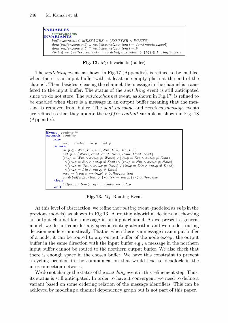
246 M. Kamali et al.
VARIABLESbuffer content
INVARIANTSbuffer content ∈ MESSAGES �→ (ROUTER × PORTS)dom(buffer content) ∪ ran(channel content) = dom(moving pool)dom(buffer content) ∩ ran(channel content) = ∅∀b ·b ∈ ran(buffer content)⇒ card(buffer content � {b}) ∈ 1 .. buffer size
Fig. 12. M2: Invariants (buffer)
The switching event, as shown in Fig.17 (Appendix), is refined to be enabledwhen there is an input buffer with at least one empty place at the end of thechannel. Then, besides releasing the channel, the message in the channel is trans-fered to the input buffer. The status of the switching event is still anticipatedsince we do not store. The out to channel event, as shown in Fig.17, is refined tobe enabled when there is a message in an output buffer meaning that the mes-sage is removed from buffer. The sent message and received message eventsare refined so that they update the buffer content variable as shown in Fig. 18(Appendix).
Event routing =extends routing
anymsg router in p out p
wherein p ∈ {Win, Ein, Sin, Nin, Uin, Din, Lin}out p ∈ {Wout, Eout, Sout, Nout, Uout, Dout, Lout}(in p = Win ∧ out p �= Wout) ∨ (in p = Ein ∧ out p �= Eout)∨(in p = Sin ∧ out p �= Sout) ∨ (in p = Nin ∧ out p �= Nout)∨(in p = Uin ∧ out p �= Uout) ∨ (in p = Din ∧ out p �= Dout)∨(in p = Lin ∧ out p �= Lout)
msg �→ (router �→ in p) ∈ buffer contentcard(buffer content � {router �→ out p}) < buffer size
thenbuffer content(msg) := router �→ out p
end
Fig. 13. M2: Routing Event
At this level of abstraction, we refine the routing event (modeled as skip in theprevious models) as shown in Fig.13. A routing algorithm decides on choosingan output channel for a message in an input channel. As we present a generalmodel, we do not consider any specific routing algorithm and we model routingdecision nondeterministically. That is, when there is a message in an input bufferof a node, it can be routed to any output buffer of the node except the outputbuffer in the same direction with the input buffer e.g., a message in the northerninput buffer cannot be routed to the northern output buffer. We also check thatthere is enough space in the chosen buffer. We have this constraint to preventa cycling problem in the communication that would lead to deadlock in theinterconnection network.
We do not change the status of the switching event in this refinement step. Thus,its status is still anticipated. In order to have it convergent, we need to define avariant based on some ordering relation of the message identifiers. This can beachieved by modeling a channel dependency graph but is not part of this paper.

Refinement-Based Modeling of 3D NoCs 247
A more concrete 3D NoC design can be modeled by refining one or more ofthese three general models and by verifying whether the design can guarantee theoverall communication correctness. In the following, we model the XYZ routingalgorithm by refining the third model M2 and verifying whether it guaranteesthe overall communication correctness.
4 Case Study: The XYZ Routing Algorithm
In this section, we formally develop a dimension-order routing (DOR) algorithmwhich is a deterministic routing scheme widely used for NoCs [24]. To make thebest use of the regularity of the topology, the dimension-order routing transferspackets along minimal paths in the traversing of the low dimension first until nofurther move is needed in this dimension. Then, they go along the next dimensionand so forth until they reach their destination. For example, the dimension-order routing in the 3D NoC called the XYZ routing algorithm uses Z dimensionchannels after using Y and X dimension channels. Packets travel along the Xdimension, then along the Y dimension and finally along the Z dimension. Thus,if current node = (cx, cy, cz) is a node containing a message addressed to nodedestination = (dx, dy, dz), then the XYZ routing function Rxyz(, ) is defined asfollows:
Rxyz((cx, cy, cz), (dx, dy, dz)) =
⎧⎪⎪⎪⎪⎪⎨⎪⎪⎪⎪⎪⎩
(cx−1, cy, cz) iff cx > dx
(cx+1, cy, cz) iff cx < dx
(cx, cy−1, cz) iff cx = dx ∧ cy > dy
(cx, cy+1, cz) iff cx = dx ∧ cy < dy
(cx, cy, cz−1) iff cx = dx ∧ cy = dy ∧ cz > dz
(cx, cy, cz+1) iff cx = dx ∧ cy = dy ∧ cz < dz
In order to model the XYZ routing algorithm based on the third general model,we have to refine the routing event which is nondeterministically defined. Asshown in the above formula, a message can be transfered to six different di-rections based on its current position and destination. Therefore, we refine therouting event in the previous model to six routing events so that their guardsare based on the routing formula. As an example of the routing event, we showin Fig.14 the situation where cx is greater than dx. All the correctness propertiesdefined for the abstract models are proved. Hence, the XYZ routing algorithmguarantees the overall communication correctness.
Event routing X dec =extends routing
wherecoordX (router) > coordX (des(msg))∧ out p = Wout
thenbuffer content(msg) := router �→ out p
end
Fig. 14. The XYZ Model: Routing Event (cx > dx)

248 M. Kamali et al.
5 Verification of the Models
In order to prove that the models satisfy their correctness properties we have tocheck that they respect their invariants, i.e., the pool properties for our models.To prove this, we have generated the proof obligations for all the models usingthe Rodin tool: part of the proof obligations were automatically discharged andthe rest of could be proved interactively. The proof statistics for our models areshown in Table 1. These figures express the number of proof obligations gener-ated by the Rodin platform as well as the number of obligations automaticallydischarged by the platform and those interactively proved. A high number of in-teractive proofs were due to reasoning about set comprehension and unions, notcurrently supported automatically in Rodin. In addition, the interactive provingoften involved manually suggesting values to discharging various properties con-taining logical disjunctions or existential quantifiers. Extra proving was due tothe fact that currently, we cannot create proof scripts and reuse them wheneverneeded in RODIN. Thus, in some cases we had to manually repeat very similaror almost identical proofs.
Table 1. Proof Statistics
Model Number of Proof Automatically Interactively
Obligations Discharged Discharged
Context 21 6(28%) 15(72%)
M0 Model 38 34(89%) 4(11%)
M1 Model 33 11(33%) 22(67%)
M2 Model 33 7(21%) 26(79%)
XYZ Model 13 0(0%) 13(100%)
Total 144 64(45%) 80(55%)
6 Conclusions
In this paper, we have proposed the abstract models M0, M1, and M2 at threeincreasing levels of detail for 3D NoCs. These can be used for modeling andverifying 3D NoC-designs in the early stages of the system development. Wehave also shown how to apply such an abstract model to verify a concrete 3DNoC routing algorithm. Most importantly, the overall correctness of the com-munication models (expressed using a special data structure called pool [2]) isguaranteed for the 3D NoCs. We have achieved this by modeling the correct-ness condition via invariants; as each model added detail to the previous model,the invariant needed to reflect these added details in a consistent manner. Inorder for the invariant to be satisfied by a model, a number of proof obliga-tions needs to be discharged. Moreover, in order for the models to respect therefinement relation M0 � M1 � M2, i.e., to develop each other in a provably

Refinement-Based Modeling of 3D NoCs 249
correct manner, some other proof obligations need to be generated. As we haveemployed the RODIN platform to specify our 3D NoC modeling, many of theseproof obligations have been automatically discharged, while for the rest it waspossible to discharge them interactively. We note an interesting property of ourcommunication correctness condition, that essentially reduces to the fact that allthe messages will eventually reach their destinations. This is a typical livenessproperty that we model here as an invariant, also based on the variant expressionensuring that our models will eventually terminate. The liveness property canalso be verified via a model checker, for instance Pro-B [31], that is associatedto the RODIN platform.
The NoC communication can be either unicast or multicast [23]. In the unicastcommunication a message is sent from a source node to a single destination node,while in the multicast communication a message is sent from a source node to anarbitrary set of destination nodes. We have considered here sending a messagefrom a source to a single destination, hence modeled unicast communication. Oneof our future plans is to extend the abstract models M0, M1, and M2 to alsospecify multicast communication and as a case study we target a novel routingprotocol for multicast traffic called HAMUM [12], based on the extended 3DNoC model. HAMUM, Hamiltonian Adaptive path for both the Multicast andUnicast Model, is a new adaptive routing model based on Hamiltonian path forboth the multicast and unicast traffic. An interesting property that we expectout of the multicast modeling is to have the case study reusing the M2 modelvia an algorithmic refinement instead of a superposition one like we now have.This is because we can have several messages that could be routed in parallelusing different events via several channels. Our XYZ routing employs alreadyseveral events for the routing instead of the abstract routing event of the modelM2, but only one of them is enabled at all moments.
By strengthening the invariants we can verify more diverse properties of the3D NoC designs, for instance we could prove deadlock-freedom for routing al-gorithms - currently, one of the most challenging properties for the 3D NoCs.For this, we envision an extension of the abstract 3D NoC models with an ex-tra channel dependency graph to reason about deadlock-freedom; the HAMUMalgorithm can then be shown as deadlock-free.
References
1. Abrial, J.R.: A System Development Process with Event-B and the Rodin Platform.In: Butler, M., Hinchey, M.G., Larrondo-Petrie, M.M. (eds.) ICFEM 2007. LNCS,vol. 4789, pp. 1–3. Springer, Heidelberg (2007)
2. Abrial, J.R.: Modeling in Event-B: System and Software Design. Cambridge Uni-versity Press (2010)
3. Abrial, J.R.: The B-Book: Assigning Programs to Meanings. Cambridge UniversityPress (1996)
4. Abrial, J.R., Cansell, D., Mery, D.: Refinement and Reachability in Even-B. In:4th International Conference of B and Z Users, pp. 129–148 (2005)

250 M. Kamali et al.
5. Abrial, J.R., Hallerstede, S.: Refinement, Decomposition and Instantiation of Dis-crete Models: Application to Event-B. In: Fundamenta Informaticae, pp. 1–28(2007)
6. Andreasson, D., Kumar, S.: Slack-Time Aware-Routing in NoC Systems. In: IEEEInternational Symposium on Circuits and Systems, pp. 2353–2356. IEEE (2005)
7. Arditi, L., Berry, G., Kishinevsky, M.: Late Design Changes (ECOs) for Sequen-tially Optimized Esterel Designs. In: Hu, A.J., Martin, A.K. (eds.) FMCAD 2004.LNCS, vol. 3312, pp. 128–143. Springer, Heidelberg (2004)
8. Back, R.J., Sere, K.: Stepwise Refinement of Action Systems. In: van de Snepscheut,J.L.A. (ed.) MPC 1989. LNCS, vol. 375, pp. 115–138. Springer, Heidelberg (1989)
9. Back, R.J., Sere, K.: Superposition Refinement of Reactive Systems. Formal As-pects of Computing 8(3), 324–346 (1996)
10. Borrione, D., Helmy, A., Pierre, L., Schmaltz, J.: A Formal Approach to the Ver-ification of Networks on Chip. EURASIP Journal on Embedded Systems 2009(1),1–14 (2009)
11. Duan, X., Zhang, D., Sun, X.: A Condition of Deadlock-free Routing in Mesh Net-work. In: Second International Conference on Intelligent Networks and IntelligentSystems, pp. 242–245 (2009)
12. Ebrahimi, M., Daneshtalab, M., Liljeberg, P., Tenhunen, H.: HAMUM A NovelRouting Protocol for Unicast and Multicast Traffic in MPSoCs. In: The 18th Eu-romicro Conference on Parallel, Distributed and Network-Based Computing (2010)
13. Feero, B.S., Pande, P.: Networks-on-Chip in a Three-Dimensional Environment: APerformance Evaluation. IEEE Transactions on Computers, 32–45 (2009)
14. Grecu, C., et al.: A Scalable Communication-Centric SoC Interconnect Architec-ture. In: 5th International Symposiom Quality Electronic Design (ISQED 2004),pp. 343–348 (2004)
15. Gupta, R., Guernic, P.L., Skuhla, S.K.: Formal methods and models for systemdesign: a system level perspective. Kluwer Academic Publishers (2004)
16. Harrison, J.: Formal Verification at Intel. In: Symposium on Logic in ComputerScience (2003)
17. Jerger, N.E., Peh, L.S., Lipasti, M.H.: Virtual Circuit Tree Multicasting: A Casefor On-Chip Hardware Multicast Support. In: International Conference ComputerArchitecture, China, pp. 229–240 (2008)
18. Katz, S.: A Superimposition Control Construct for Distributed Systems. ACMTransactions on Programming Languages and Systems, 337–356 (1993)
19. Kaivola, R., Ghughal, R., Narasimhan, N., Telfer, A., Whittemore, J., Pandav,S., Slobodova, A., Taylor, C., Frolov, V., Reeber, E., Naik, A.: Replacing Testingwith Formal Verification in Intel� CoreTM i7 Processor Execution Engine Valida-tion. In: Bouajjani, A., Maler, O. (eds.) CAV 2009. LNCS, vol. 5643, pp. 414–429.Springer, Heidelberg (2009)
20. Kim, Y.B., Kim, Y.-B.: Fault-Tolerant Source Routing for Networks-on-Chip. In:22nd IEEE International Symposium on Defect and Fault Tolerance in VLSI Sys-tems, pp. 12–20. IEEE Computer Society (2007)
21. Liao, W., Hsiung, P.: Creating a Formal Verification Platform for IBMCoreConnect-based SoC. In: The 1st International Workshop on Automasted Tech-nology for Verificatin and Analysis (ATVA 2003), pp. 7–18 (2003)
22. Loi, I., Benini, L.: An Efficient Distributed Memory Interface for Many-Core Plat-form with 3D Stacked DRAM. In: Proc. of the DATE Conference, Germany,pp. 99–104 (2010)

Refinement-Based Modeling of 3D NoCs 251
23. Lu, Z., Yin, B., Jantsch, A.: Connection-Oriented Multicasting in Wormhole-Switched Networks on Chip. In: Emerging VLSI Technologies and Architectures,pp. 205–211 (2006)
24. Montaana, J.M., Koibuchi, M., Matsutani, H., Amano, H.: Balanced Dimension-Order Routing for k-ary n-cubes. In: International Conference on Parallel Process-ing (2009)
25. Nayebi, A., Meraji, S., Shamaei, A., Sarbazi-azad, H.: XMulator: A listener-BasedIntegrated Simulation Platform for Interconnection Networks. In: Asia Interna-tional Conference on Modeling and Simulation, pp. 128–132 (2007)
26. Palesi, M., Holsmark, R., Kumar, S., Catania, V.: Application Specific RoutingAlgorithms for Networks on Chip. IEEE Transactions on Parallel and DistributedSystems, 316–330 (2009)
27. Park, D., et al.: Mira, A Multi-Layered On-Chip Interconnect Router Architecture.In: ISCA 2008, pp. 251–261 (2008)
28. Tsiopoulos, L., Walden, M.: Formal Development of NoC Systems in B. NordicJournal of Computing, 127–145 (2006)
29. Yan, S., Lin, B.: Design of Application-Specific 3D Networks-on-Chip Architec-tures. In: IEEE International Conference on Computer Design (ICCD 2008),pp. 142–149 (2008)
30. RODIN Tool Platform, http://www.event-b.org/platform.html31. ProB Model Checker, http://www.stups.uni-duesseldorf.de/ProB/overview.php

252 M. Kamali et al.
Appendix
Event out to channel =any new position current msg out p in pwhere
current msg ∈ dom(moving pool) ∧ new position ∈ POSITIONmoving pool(current msg) �→ new position ∈ Neighout p ∈ {Nout, Sout, Wout, Eout, Uout, Dout} ∧ in p ∈ {Nin, Sin, Win, Ein, Uin, Din}(moving pool(current msg) �→ out p) �→ (new position �→ in p) ∈ dom(mk channel)channel state(mk channel((moving pool(current msg)�→out p)�→(new position �→in p)))= freemoving pool(current msg) �= des(current msg) ∧ current msg /∈ ran(channel content)
thenchannel state(mk channel((moving pool(current msg)�→out p)�→(new position �→in p))):=busychannel content(mk channel((moving pool(current msg) �→out p) �→ (new position �→ in p)))
:= current msgend
Fig. 15. M1: Out to Channel Event
Event switching =Status anticipatedextends switchingany current msg new position p1 p2where
p1 ∈ {Nout, Sout, Wout, Eout, Uout, Dout} ∧ p2 ∈ {Nin, Sin, Win, Ein, Uin, Din}(moving pool(current msg) �→ p1 ) �→ (new position �→ p2 ) ∈ dom(mk channel)channel state(mk channel((moving pool(current msg)�→p1 )�→(new position �→p2 )))=busycurrent msg =channel content(mk channel((moving pool(current msg) �→p1 ) �→ (new position �→p2 )))
thenmoving pool(current msg) := new positionchannel state(mk channel((moving pool(current msg)�→p1 )�→(new position �→p2 ))) := freechannel content := channel content �− {current msg}
end
Fig. 16. M1: Switching Event
Event switching =Status anticipatedextends switching
wherecard(buffer content � {new position �→ p2}) < buffer size
thenbuffer content := buffer content ∪ {current msg �→ (new position �→ p2 )}
endEvent out to channel =extends out to channel
wherecard(buffer content � {new position �→ in p}) > 0
thenbuffer content :=buffer content\{current msg �→ (moving pool(current msg) �→out p)}
end
Fig. 17. M2: Switching and Out to Channel Events
Event sent message =extends sent message
wherecurrent msg /∈ dom(buffer content)
thenbuffer content := buffer content ∪ {current msg �→ (src(current msg) �→ Lin)}
endEvent received message =extends received message
wherecurrent msg �→ (des(current msg) �→ Lout) ∈ buffer content
thenbuffer content := buffer content \ {current msg �→ (des(current msg) �→ Lout)}
end
Fig. 18. M2: Sent message and Received message Events


Paper VI
Formal Modeling of Multicast Communication in
3D NoCs
Maryam Kamali, Luigia Petre, Kaisa Sere
and Masoud Daneshtalab
Originally published in: P. Kitsos and S. Niar (Eds.), Proceedings of the 14thEuromicro Conference on Digital System Design - DSD 2011, pp. 634-642.IEEE/Euromicro, August 2011.
157


Formal Modeling of Multicast Communication in3D NoCs
Maryam Kamali∗†, Luigia Petre∗, Kaisa Sere∗ and Masoud Daneshtalab‡∗Abo Akademi University, Finland
Email: {maryam.kamali,luigia.petre,kaisa.sere}@abo.fi†Turku Centre for Computer Science (TUCS), Finland
‡University of Turku, FinlandEmail: [email protected]
Abstract—A reliable approach to designing systems is byapplying formal methods, based on logics and set theory. Informal methods refinement based, we develop the system modelsstepwise, from an abstract level to a concrete one by graduallyadding details. Each detail-adding level is proved to still validatethe properties of the more abstract level. Due to the highcomplexity and the high reliability requirements of 3D NoCs,formal methods provide promising solutions for modeling andverifying their communication schemes. In this paper, we presenta general model for specifying the 3D NoC multicast communi-cation scheme. We then refine our model to two communicationschemes,: unicast and multicast, via the XYZ routing algorithmin order to put forward the correct-by-construction concretemodels.
Index Terms—Formal methods; Event-B; refinement; 3D NoC;multicast communication
I. INTRODUCTION
The Network-on-Chip (NoC) architecture paradigm, basedon a modular packet-switching mechanism, can address manyof the on-chip communication design issues such as per-formance limitations of long interconnects and the integra-tion of high numbers of Intellectual Property (IP) cores ona chip. However, the 2D-chip fabrication technology facesmany challenges in the deep submicron regime even whenemploying NoC architectures. Examples of these problems arethe design of the clock-tree network for large chips, limitedfloor-planning choices, the increase of both the wire delay andpower consumption, the integration of various components thatare digital, analog, MEMS and RF, etc. Three Dimensional In-tegrated Circuits (3D ICs) have been emerging as an attractivecandidate, for the reduction of interconnection length and theadded interconnect scalability in the third dimension offer anopportunity to further improve the performance of NoC [13],[15], [14].
Three dimensional Networks-on-Chips (3D NoCs) [13]provide more reliable interconnections due to the increasednumber of links between components. Due to their promiseof parallelism and efficiency, 3D NoCs have a critical role inleading towards reliable computing platforms. However, themajority of their evaluation approaches are simulation-basedtools, such as XMulator [16], Noxim [17], etc. Simulation-based approaches are usually applied in the late stages ofdesign and are limited, e.g., by the length of time that a
system is simulated. This means that exhaustive checking ofall the system states is impossible in practice for complex 3DNoCs and thus, simulation is not suitable for verifying thecorrectness of a NoC design.
Another approach to address this problem is via formalmethods. Formal methods refer to the application of mathe-matical techniques to the design and implementation of com-puter hardware and software. Prominent examples of applyingformal methods are provided by, e.g., Intel [19], [18] andIBM [21] for formally verifying hardware or systems-on-chip(SoC) [20]. By using rigorous mathematical techniques, it ispossible to deliver provably correct systems. Formal methodsare based on the capture of system requirements in a specific,precise format. Importantly, such a format can be analyzedfor various properties and, if the formal method permits, alsostepwise developed until an implementation is formed. Byfollowing such a formal development, we are sure that the finalresult correctly implements the requirements of the system.
A general formal model of 3D NoCs was recently intro-duced in [12], to verify the design of unicast communicationapproaches. Unicast communication refers to sending a mes-sage from a single source node to a single destination node. Inthis paper we extend the proposed model to a general formalmodel of 3D NoCs for specifying and verifying the designof multicast communication. We show that the unicast modelin [12] is an instance of our general model in this paper.
Communication in network-based multicore architecturescan be either unicast (one-to-one) or multicast (one-to-many) [22]. While in the former approach a message issent from a source node to a single destination node, inthe latter approach a message is sent from a source nodeto an arbitrary set of destinations. Multicast communicationis employed in many multicore applications, e.g., replication,barrier synchronization, cache coherency in distributed shared-memory architectures, and clock synchronization [22], [23].Multicast routing algorithms can be classified as unicast-based, tree-based, and path-based [25]. The first alternativeproduces much unnecessary traffic, also increasing the latencyand congestion of the network [25]. The path-based methodforces packets to follow longer routes than what is proposedin the tree-based method, hence the tree-based method seemsthe most efficient of the three [26].
2011 14th Euromicro Conference on Digital System Design
978-0-7695-4494-6/11 $26.00 © 2011 IEEE
DOI 10.1109/DSD.2011.86
634
2011 14th Euromicro Conference on Digital System Design
978-0-7695-4494-6/11 $26.00 © 2011 IEEE
DOI 10.1109/DSD.2011.86
634
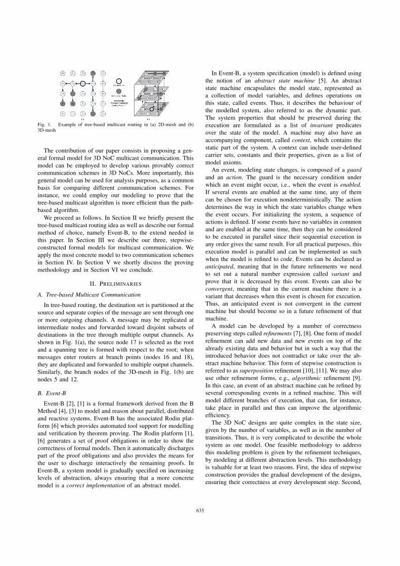
Fig. 1. Example of tree-based multicast routing in (a) 2D-mesh and (b)3D-mesh
The contribution of our paper consists in proposing a gen-eral formal model for 3D NoC multicast communication. Thismodel can be employed to develop various provably correctcommunication schemes in 3D NoCs. More importantly, thisgeneral model can be used for analysis purposes, as a commonbasis for comparing different communication schemes. Forinstance, we could employ our modeling to prove that thetree-based multicast algorithm is more efficient than the path-based algorithm.
We proceed as follows. In Section II we briefly present thetree-based multicast routing idea as well as describe our formalmethod of choice, namely Event-B, to the extend needed inthis paper. In Section III we describe our three, stepwise-constructed formal models for multicast communication. Weapply the most concrete model to two communication schemesin Section IV. In Section V we shortly discuss the provingmethodology and in Section VI we conclude.
II. PRELIMINARIES
A. Tree-based Multicast Communication
In tree-based routing, the destination set is partitioned at thesource and separate copies of the message are sent through oneor more outgoing channels. A message may be replicated atintermediate nodes and forwarded toward disjoint subsets ofdestinations in the tree through multiple output channels. Asshown in Fig. 1(a), the source node 17 is selected as the rootand a spanning tree is formed with respect to the root; whenmessages enter routers at branch points (nodes 16 and 18),they are duplicated and forwarded to multiple output channels.Similarly, the branch nodes of the 3D-mesh in Fig. 1(b) arenodes 5 and 12.
B. Event-B
Event-B [2], [1] is a formal framework derived from the BMethod [4], [3] to model and reason about parallel, distributedand reactive systems. Event-B has the associated Rodin plat-form [6] which provides automated tool support for modellingand verification by theorem proving. The Rodin platform [1],[6] generates a set of proof obligations in order to show thecorrectness of formal models. Then it automatically dischargespart of the proof obligations and also provides the means forthe user to discharge interactively the remaining proofs. InEvent-B, a system model is gradually specified on increasinglevels of abstraction, always ensuring that a more concretemodel is a correct implementation of an abstract model.
In Event-B, a system specification (model) is defined usingthe notion of an abstract state machine [5]. An abstractstate machine encapsulates the model state, represented asa collection of model variables, and defines operations onthis state, called events. Thus, it describes the behaviour ofthe modelled system, also referred to as the dynamic part.The system properties that should be preserved during theexecution are formulated as a list of invariant predicatesover the state of the model. A machine may also have anaccompanying component, called context, which contains thestatic part of the system. A context can include user-definedcarrier sets, constants and their properties, given as a list ofmodel axioms.
An event, modeling state changes, is composed of a guardand an action. The guard is the necessary condition underwhich an event might occur, i.e., when the event is enabled.If several events are enabled at the same time, any of themcan be chosen for execution nondeterministically. The actiondetermines the way in which the state variables change whenthe event occurs. For initializing the system, a sequence ofactions is defined. If some events have no variables in commonand are enabled at the same time, then they can be consideredto be executed in parallel since their sequential execution inany order gives the same result. For all practical purposes, thisexecution model is parallel and can be implemented as suchwhen the model is refined to code. Events can be declared asanticipated, meaning that in the future refinements we needto set out a natural number expression called variant andprove that it is decreased by this event. Events can also beconvergent, meaning that in the current machine there is avariant that decreases when this event is chosen for execution.Thus, an anticipated event is not convergent in the currentmachine but should become so in a future refinement of thatmachine.
A model can be developed by a number of correctnesspreserving steps called refinements [7], [8]. One form of modelrefinement can add new data and new events on top of thealready existing data and behavior but in such a way that theintroduced behavior does not contradict or take over the ab-stract machine behavior. This form of stepwise construction isreferred to as superposition refinement [10], [11]. We may alsouse other refinement forms, e.g., algorithmic refinement [9].In this case, an event of an abstract machine can be refined byseveral corresponding events in a refined machine. This willmodel different branches of execution, that can, for instance,take place in parallel and thus can improve the algorithmicefficiency.
The 3D NoC designs are quite complex in the state size,given by the number of variables, as well as in the number oftransitions. Thus, it is very complicated to describe the wholesystem as one model. One feasible methodology to addressthis modeling problem is given by the refinement techniques,by modeling at different abstraction levels. This methodologyis valuable for at least two reasons. First, the idea of stepwiseconstruction provides the gradual development of the designs,ensuring their correctness at every development step. Second,
635635

Fig. 2. Model development for multicast communication
the abstract models can contain non-determinism, which al-lows that in the subsequent models we simply fix the choice toone specific execution. Obviously, in this case, we can developalternative models corresponding to different (fixed) choices,all refining the same abstract model.
III. THREE ABSTRACT MODELS FOR MULTICASTCOMMUNICATION
In this section we formally develop three high-level modelsM0, M1, and M2 for the 3D NoC. Our models are at threeincreasing levels of detail so that each model is a refinementof the previous one: M0 �M1 � M2 as shown in Fig. 2. Westart by building a model that is far more abstract than thefinal network we want to construct. The idea is to take intoaccount initially only very few constraints. This is because wewant to be able to reason about this system in a simple way,considering in turn each element of the network. Therefore, inthe initial model, we specify a network of nodes as a contextand define the correctness properties of this network based ona specific data structure called pool, as suggested by [2]. Inthe second model, we refine the initial model by adding newdata and events to model the 3D mesh-based NoC architecture;besides, we specify the channels between nodes. In the thirdmodel, we model buffers for nodes and refine the commu-nication model by considering the correctness properties ofthe network. This design strategy lets us add complexity tothe model based on the correctness properties of the network,defined abstractly already in the initial model.
A. The initial model M0
The first model M0 that we construct is rather abstract:we do not consider the numerous parts of the network suchas channels or buffers; they will be introduced in subsequentrefinements. M0 will thus allow us to reason about the systemvery abstractly [2]. The model M0 is formed of the static part(ctx1) and the dynamic part (M0), as follows.
The static part of our model describes the network structurein terms of neighbors and the messages to travel through thenetwork. We model the network structure with a relation Neighon the finite and non-empty ROUTER set; this relation denotesthe communication links among nodes, expressed with themany to many mapping relation operator ↔. We model themessages to travel through the network with a finite, non-empty set MESSAGES. A message is modeled as a triple
Fig. 3. Multicast Message Pools
(data, source, destinations), where data is an element of thefinite and non-empty DATA set (modeling the information totransmit), source is an element of the set ROUTER where amessage is injected, and destinations is a subset of the setROUTER where a message should be received. We definetwo functions, named src and des that return source anddestinations, respectively. The detailed properties of thesestructures are formally introduced in [12], where they onlyhad a different type of destination. The modification we needfor modeling multicast refers to defining the MESSAGESset, expressed with the total function operator →, as follows:
MESSAGES∈ DATA→ROUTER→P(ROUTER)Neigh ∈ ROUTER↔ROUTERsrc∈MESSAGES→ROUTERdes∈ MESSAGES→P(ROUTER)In our network model we use the following condition
for modeling the communication correctness: the messagesin the network will eventually reach their destinations. Toimplement this condition in our multicast communicationscheme, we define two message subsets, one message-to-node relation and one node-to-message relation as machinevariables: sent pool ⊆ MESSAGES, received pool ⊆MESSAGES, moving pool∈sent pool↔ROUTER andreceived node∈ROUTER↔sent pool.
The map moving pool models the current position ofmessages which are routed in the network. In [12], there isonly one instance of a message in the network; therefore,moving pool is defined as a (partial) function. However, inthis paper, we model moving pool as a relation of messages-to-nodes to show the existence of a number of instances of amessage in different nodes. In order to show that a messageis received to all its destinations, we define a new relationreceived node∈ROUTER ↔ MESSAGES which mod-els instances of messages having reached destinations. When amessage is received to one of its destinations, a correspondingmap is added to the received node relation. In order tohave a message in received pool, which denotes the list ofreceived messages, a destination-to-message map for all of thedestinations of that message should be in received node. Thenew message pool structure is illustrated in Fig. 3.
One of the working steps of multicast communication isto replicate a message in intermediate or destination nodes.When a message is received to a node the message can beconsumed and forwarded to one or several immediate neigh-bors or consumed and removed from the network. Therefore,we can produce multiple instances of a message in a nodeand switch these instances to different neighbors. In order to
636636

Event sent messageany current msgwhere
current msg ∈ MESSAGEScurrent msg /∈ sent pool
thensent pool := sent pool ∪ {current msg}moving pool :=moving pool∪{current msg �→src(current msg)}replicate msg num(current msg �→ src(current msg)) := 0replicate flag(current msg �→ src(current msg)) := FALSE
end
Fig. 4. M0: sent message Event
model the message replication in nodes, we define two newvariables: replicate flag ∈ moving pool → BOOL andreplicate msg num ∈ moving pool → 0..n − 1 (where nis the maximum number of node neighbors; we assume this isa constant of the model). When replicate flag returns falsefor a pair of (node, message), this means that the messageis received to a node but it is not replicated yet. Whenreplicate flag returns true for a pair of (node, message),this models that the message which is received to the node isreplicated. In this case, the number of message replicas in thenode is expressed with replicate msg num.
To model the communication and the message pool func-tions, we add five more events to the unicast model thanpreviously developed in [12]. In the following, we summarizethe already defined events with the changes as well as the newevents. The sent message event handles the injection of anew message into the network. As shown in Fig. 4, whenever amessage is injected into the network, both sent pool as well asmoving pool are updated. Moreover, the pair of (source node,message) with the value false is added to the replicate flagto show the existence of a message in the source node withno replication yet.
A message in moving pool should be routed toward itsdestination. This is composed of three actions, one for decidingwhich node would be the next one (routing), the other forreplicating a message to a number of instances of the message(replicating), and the last for transferring the message tothat node (switching). These three actions are available forall the nodes, including the source, the destination as wellas all the intermediate nodes and are modeled respectivelyby the routing, replicating, and four switching events.The routing event consists of skip at this abstract level asrouting decisions are modeled only when a particular routingalgorithm is needed to be verified; we then add the routing asa refinement to this abstract model.
The replicating event shown in Fig. 5 handles the repli-cation of a message in a node. When a message arrives to anode, the replicating event becomes enabled for that nodeand the message and a random number between 0 and n-1 isassigned to the pair (node, message) in replicate msg num.The assigned number is nondeterministically chosen, becauseit makes our initial model general and reusable for a vari-ety of communication design schemes. The number will beassigned deterministically when the model is refined to aparticular communication design. We illustrate this in Section
Event replicatingany current msg pos numwhere
current msg �→ pos ∈ moving poolreplicate flag(current msg �→ pos) = FALSEreceived node−1[{current msg}] ∪ {pos} ⊂ des(current msg)num ∈ 0 .. 6
thenreplicate flag(current msg �→ pos) := TRUEreplicate msg num(current msg �→ pos) := num
end
Fig. 5. M0: replicating Event
Event switchingany current msg pos new positionwhere
current msg �→ pos ∈ moving poolpos /∈ des(current msg)new position �→ pos ∈ Neighnew position �= src(current msg)replicate flag(current msg �→ pos) = TRUEreplicate msg num(current msg �→ pos) > 0current msg �→ new position /∈ moving poolcurrent msg /∈ received node[{new position}]
thenmoving pool := moving pool ∪ {current msg �→ new position}replicate flag := replicate flag∪
{current msg �→ new position �→ FALSE}replicate msg num :=({current msg �→pos}�−replicate msg num)
∪{current msg �→ pos �→ (replicate msg num(current msg �→pos)−1), current msg �→ new position �→ 0}
end
Fig. 6. M0: switching Event
IV with the XYZ routing case study. When the number ofreplication for a message in a node is selected, the instancesof the message should be transfered from the current nodeto its neighbors nondeterministically and the moving pool,received node, replicate msg num and replicate flagfor the message instances should be updated.
Because different states are possible for switching, theswitching function is splitted in four switching events:Switching, switching removing, switching garbage andswitching removing garbage.
Two possible states of switching occur when the transferringmessage is not the last replicated instance and when thetransferring message is the last one. When it is not the lastinstance, the switching event as illustrated in Fig. 6 transfersthe message to the next node by adding the pair (next node,message) to the moving pool and decreasing the number ofreplicated instances in the current node. The replicate flagof the message and the new position are updated to false.The false value of replicate flag for a message and a nodeexpresses the receipt of a new message. When a messageis the last replicated instance of a message in a node, theswitching removing event illustrated in Fig. 7 transfers themessage to the next node by adding (next node, message)and removing the previous (node, message) pairs to/frommoving pool. In addition, the previous (node, message) pairis removed from replicate flag and replicate msg num,expressed with the domain subtraction operator �−.
If the next node has already received a message fromits other neighbors but the same message is switch-
637637

Event Switching removingany current msg new position poswhere
current msg �→ pos ∈ moving poolpos /∈ des(current msg)new position �→ pos ∈ Neighnew position �= src(current msg)replicate flag(current msg �→ pos) = TRUEreplicate msg num(current msg �→ pos) = 0current msg �→ new position /∈ moving poolcurrent msg /∈ received node[{new position}]
thenmoving pool := (moving pool \ {current msg �→ pos})
∪{current msg �→ new position}replicate flag := ({current msg �→ pos}�− replicate flag)
∪{current msg �→ new position �→ FALSE}replicate msg num := ({current msg �→ pos}�−
replicate msg num)∪{current msg �→ new position �→ 0}end
Fig. 7. M0: switching removing Event
Event switching garbageany current msg pos new positionwhere
current msg �→ pos ∈ moving poolpos /∈ des(current msg)new position �→ pos ∈ Neighnew position �= src(current msg)replicate flag(current msg �→ pos) = TRUEreplicate msg num(current msg �→ pos) > 0current msg �→ new position ∈ moving pool∨
current msg ∈ received node[{new position}]then
replicate msg num :=({current msg �→pos}�−replicate msg num)∪{current msg �→ pos �→ (replicate msg num(current msg �→pos)−1), current msg �→ new position �→ 0}
end
Fig. 8. M0: switching garbage Event
ing in the next node, then the message from the pre-vious node is removed from the network since it rep-resent duplication. The switching garbage (Fig.8) andswitching removing garbage (Fig. 9) events handle thesame situations as switching and switching removingevents with the difference that the received message to a nextnode is not added to the moving pool because the messageis an extra instance of a message.
The received message event in the unicast model addsa message received at its destination to received pool andremoves the message from moving pool. This event is splitted
Event switching removing garbageany current msg pos new positionwhere
current msg �→ pos ∈ moving poolpos /∈ des(current msg)new position �→ pos ∈ Neighnew position �= src(current msg)replicate flag(current msg �→ pos) = TRUEreplicate msg num(current msg �→ pos) = 0current msg �→ new position ∈ moving pool∨
current msg ∈ received node[{new position}]then
moving pool := (moving pool \ {current msg �→ pos})replicate flag := ({current msg �→ pos}�− replicate flag)replicate msg num :=({current msg �→pos}�−replicat msg num)
end
Fig. 9. M0: switching removing garbage Event
Event received messageany current msg poswhere
received node−1[{current msg}] ∪ {pos} ⊂ des(current msg)current msg �→ pos ∈ moving poolreplicate flag(current msg �→ pos) = TRUEreplicate msg num(current msg �→ pos) > 0pos �→ current msg /∈ received node
thenreceived node := received node ∪ {pos �→ current msg}
end
Fig. 10. M0: received message Event
Event complete received messageany current msg poswhere
current msg �→ pos ∈ moving poolpos ∈ des(current msg)received node−1[{current msg}] ∪ {pos} = des(current msg)
thenreceived node := received node ∪ {pos �→ current msg}moving pool := {current msg}�−moving poolreceived pool := received pool ∪ {current msg}replicate msg num :=({current msg}� moving pool)�−
replicate msg numreplicate flag := ({current msg}�moving pool)�−replicate flag
end
Fig. 11. M0: Complete Received message Event
into two receiving events in the multicast model: one eventmodels the case when a message is received to all its desti-nations and one events models the case when a message isreceived to one of its destinations and it still has destinationsto reach. The received message complete event handles theformer case and the received message event handles thelatter case.
The received message event illustrated in Fig. 10 adds amessage received at one of its destinations to received nodewhen at least one of the message destinations is not receivedyet. The received message complete event, illustrated inFig. 11 adds a message received at all its destinations toreceived pool and removes the message from moving pool.A message is received to all its destinations when the samenumber of destinations is in received node. This event isconvergent: if new messages are not injected to the networkfor a certain time, all the messages will be received at theirdestinations. This is proved by means of the (sent pool \received pool) variant denoting the difference between thesets sent pool and received pool.
In order to prove the communication correctness, we need toprove that received pool subset contains only messages whichare received to all of their destinations. In addition, we haveto prove that the sent pool subset eventually becomes equalwith the received pool subset and the moving pool subset isempty when all the messages are received at their destinations.These properties are illustrated in Fig. 12 as invariants.
M0 is a general specification of a general network andwill be refined to model 3D NoC multicast communicationdesigns in the following. Moreover, the model provides thenecessary properties that should be preserved by refinement.These properties, that guarantee the overall communication
638638

Invariantsreceived pool ∩ dom(moving pool) = ∅received pool ∪ dom(moving pool) = sent pool∀msg·msg ∈ dom(moving pool)⇒
(∃d·d ∈ des(msg) ∧ d �→ msg /∈ received node)∀msg·msg ∈ received pool⇒
(∀d·d ∈ des(msg)⇒ d �→ msg ∈ received node)∀msg·msg ∈ sent pool ∧ des(msg) \ received node−1[{msg}] �=∅⇒msg ∈ dom(moving pool)
Fig. 12. M0: Invariants (Pool Modeling)
Fig. 13. Router in 3D Mesh-Based NoCs
correctness, are defined as the list of invariants.
B. The Second Model M1
In the unicast model of communication presented in [12],the 3D NoC mesh-based architecture is specified by restrictingthe neighbor relation so that two nodes with coordinates(xi, yi, zi) and (xj , yj , zj) are neighbors if and only if |xi −xj |+ |yi − yj |+ |zi − zj | = 1. Based on this architecture andthe seven-port routers, the communication channels betweenrouters are defined by specifying a relation between outputand input ports of neighbors as illustrated in Fig. 13.
To show how two neighbors are connected to eachother through channels, the def channel ∈ (ROUTER ×PORTS)→ (ROUTER×PORTS) relation is defined. Thedef channel relation models the relation of a port of a nodeto the corresponding port of its neighbor. As an illustration,east and west ports of neighbor nodes with different X coor-dinates are related to each other through a channel. As shownin Fig. 14, the Ein and Eout ports of node (1, 1, 1) are con-nected to the Wout and Win ports of node (2, 1, 1) througha channel, via relations ((1, 1, 1) �→ Eout) �→ ((2, 1, 1) �→Win) and ((2, 1, 1) �→ Wout) �→ ((1, 1, 1) �→ Ein) indef channel.
Based on these channel and neighbor structures given inthe unicast model, we refine the initial model to specify thetransfering of messages through the communication channels,so that the overall correctness of communication holds.
In order to show the data transfer through the chan-nels, we specify two new variables in the secondmodel: channel state ∈ CHANNELS → state andchannel content ∈ CHANNELS �� MESSAGES. Thechannel state variable models the fact that a channel is either
Fig. 14. Channels in 3D Mesh-Based NoCs
Invariantsdom(channel content) = channel state−1[{busy}]ran(channel content) ⊆ dom(moving pool)∀msg·msg ∈ dom(moving pool) ∧ des(msg) = moving pool(msg)⇒msg /∈ ran(channel content)
Fig. 15. M1: Invariants (channels)
occupied by a message or free to transport a message; thevariable channel content indicates which message is cur-rently transferred via the channel. When a message is injectedinto a channel, its associated channel state variable is setto busy and the message is added to the channel contentvariable. We model the receipt of the message at the otherend of channel by channel state being set to free and byremoving the message from the channel content variable.
In order to construct a correct model in this refinement step,the model should satisfy the properties illustrated in Fig. 15as well as the invariants defined the initial model. The newinvariants model that, when a channel is released, its content isempty and can thus receive the next message; when a channelis busy, the message is in the channel.
In the initial model, transfering a message from a node to aneighbor node is modeled in one step while in this model it isrefined to show it in two steps through channels: first, pushinga message in the channel is modeled by a newly introducedevent out to channel and second, releasing the channel byreceiving the message at the end of the channel is modeled byextending the four switching events.
The guards of these events are strengthened with new condi-tions. Namely, these conditions check whether a channel start-ing from a node is busy, then the channel is released and thecorresponding message is removed from the channel contentand transfered to the other end of the channel, if the samemessage has not already been received there.
C. The Third Model M2
In the third model, we define node buffers by attach-ing a buffer to each port of a router. A new variablebuffer content ∈ MESSAGES ↔ (ROUTER ×PORTS) is defined to show the content of each buffer ina node. In the multicast model, several instances of a messagecan appear in several nodes, while in the unicast model onlyone instance of a message can appear in one node. Therefore,buffer content in unicast model is defined by a partialfunction while in this model we define it with a binary relation.
At this level of abstraction, we refine the routing event(modeled as skip in the previous models) as shown in Fig. 16,to route a number of instances of a message in a node.A message from an input buffer is routed to a number ofoutput buffers. The number of output buffers is equal to thenumber of instances for the pair (router, message) in thereplicate msg num relation. As we present a general model,we do not consider any specific routing algorithm and wemodel routing decisions nondeterministically. That is, whenthere is a message in an input buffer of a node, it can be routedto several output buffers of the node except the output buffer
639639
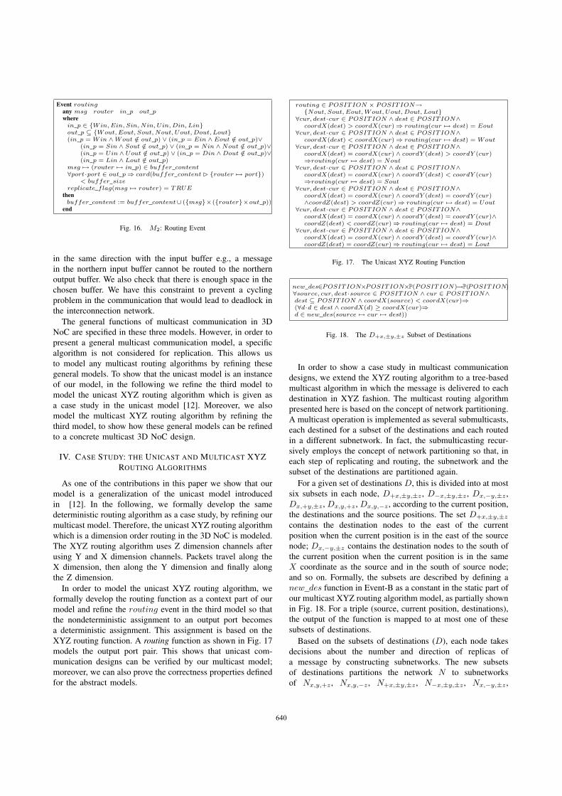
Event routingany msg router in p out pwhere
in p ∈ {Win, Ein, Sin, Nin, Uin, Din, Lin}out p ⊆ {Wout, Eout, Sout, Nout, Uout, Dout, Lout}(in p = Win ∧Wout /∈ out p) ∨ (in p = Ein ∧ Eout /∈ out p)∨
(in p = Sin ∧ Sout /∈ out p) ∨ (in p = Nin ∧Nout /∈ out p)∨(in p = Uin ∧ Uout /∈ out p) ∨ (in p = Din ∧Dout /∈ out p)∨(in p = Lin ∧ Lout /∈ out p)
msg �→ (router �→ in p) ∈ buffer content∀port·port ∈ out p⇒ card(buffer content � {router �→ port})
< buffer sizereplicate flag(msg �→ router) = TRUE
thenbuffer content := buffer content∪ ({msg}×({router}×out p))
end
Fig. 16. M2: Routing Event
in the same direction with the input buffer e.g., a messagein the northern input buffer cannot be routed to the northernoutput buffer. We also check that there is enough space in thechosen buffer. We have this constraint to prevent a cyclingproblem in the communication that would lead to deadlock inthe interconnection network.
The general functions of multicast communication in 3DNoC are specified in these three models. However, in order topresent a general multicast communication model, a specificalgorithm is not considered for replication. This allows usto model any multicast routing algorithms by refining thesegeneral models. To show that the unicast model is an instanceof our model, in the following we refine the third model tomodel the unicast XYZ routing algorithm which is given asa case study in the unicast model [12]. Moreover, we alsomodel the multicast XYZ routing algorithm by refining thethird model, to show how these general models can be refinedto a concrete multicast 3D NoC design.
IV. CASE STUDY: THE UNICAST AND MULTICAST XYZROUTING ALGORITHMS
As one of the contributions in this paper we show that ourmodel is a generalization of the unicast model introducedin [12]. In the following, we formally develop the samedeterministic routing algorithm as a case study, by refining ourmulticast model. Therefore, the unicast XYZ routing algorithmwhich is a dimension order routing in the 3D NoC is modeled.The XYZ routing algorithm uses Z dimension channels afterusing Y and X dimension channels. Packets travel along theX dimension, then along the Y dimension and finally alongthe Z dimension.
In order to model the unicast XYZ routing algorithm, weformally develop the routing function as a context part of ourmodel and refine the routing event in the third model so thatthe nondeterministic assignment to an output port becomesa deterministic assignment. This assignment is based on theXYZ routing function. A routing function as shown in Fig. 17models the output port pair. This shows that unicast com-munication designs can be verified by our multicast model;moreover, we can also prove the correctness properties definedfor the abstract models.
routing ∈ POSITION × POSITION→{Nout, Sout, Eout, Wout, Uout, Dout, Lout}
∀cur, dest·cur ∈ POSITION ∧ dest ∈ POSITION∧coordX(dest) > coordX(cur)⇒ routing(cur �→ dest) = Eout
∀cur, dest·cur ∈ POSITION ∧ dest ∈ POSITION∧coordX(dest) < coordX(cur)⇒ routing(cur �→ dest) = Wout
∀cur, dest·cur ∈ POSITION ∧ dest ∈ POSITION∧coordX(dest) = coordX(cur) ∧ coordY (dest) > coordY (cur)⇒routing(cur �→ dest) = Nout
∀cur, dest·cur ∈ POSITION ∧ dest ∈ POSITION∧coordX(dest) = coordX(cur) ∧ coordY (dest) < coordY (cur)⇒routing(cur �→ dest) = Sout
∀cur, dest·cur ∈ POSITION ∧ dest ∈ POSITION∧coordX(dest) = coordX(cur) ∧ coordY (dest) = coordY (cur)∧coordZ(dest) > coordZ(cur)⇒ routing(cur �→ dest) = Uout
∀cur, dest·cur ∈ POSITION ∧ dest ∈ POSITION∧coordX(dest) = coordX(cur) ∧ coordY (dest) = coordY (cur)∧coordZ(dest) < coordZ(cur)⇒ routing(cur �→ dest) = Dout
∀cur, dest·cur ∈ POSITION ∧ dest ∈ POSITION∧coordX(dest) = coordX(cur) ∧ coordY (dest) = coordY (cur)∧coordZ(dest) = coordZ(cur)⇒ routing(cur �→ dest) = Lout
Fig. 17. The Unicast XYZ Routing Function
new des∈POSITION×POSITION×P(POSITION)→P(POSITION)∀source, cur, dest·source ∈ POSITION ∧ cur ∈ POSITION∧dest ⊆ POSITION ∧ coordX(source) < coordX(cur)⇒(∀d·d ∈ dest ∧ coordX(d) ≥ coordX(cur)⇒d ∈ new des(source �→ cur �→ dest))
Fig. 18. The D+x,±y,±z Subset of Destinations
In order to show a case study in multicast communicationdesigns, we extend the XYZ routing algorithm to a tree-basedmulticast algorithm in which the message is delivered to eachdestination in XYZ fashion. The multicast routing algorithmpresented here is based on the concept of network partitioning.A multicast operation is implemented as several submulticasts,each destined for a subset of the destinations and each routedin a different subnetwork. In fact, the submulticasting recur-sively employs the concept of network partitioning so that, ineach step of replicating and routing, the subnetwork and thesubset of the destinations are partitioned again.
For a given set of destinations D, this is divided into at mostsix subsets in each node, D+x,±y,±z , D−x,±y,±z , Dx,−y,±z ,Dx,+y,±z , Dx,y,+z , Dx,y,−z , according to the current position,the destinations and the source positions. The set D+x,±y,±z
contains the destination nodes to the east of the currentposition when the current position is in the east of the sourcenode; Dx,−y,±z contains the destination nodes to the south ofthe current position when the current position is in the sameX coordinate as the source and in the south of source node;and so on. Formally, the subsets are described by defining anew des function in Event-B as a constant in the static part ofour multicast XYZ routing algorithm model, as partially shownin Fig. 18. For a triple (source, current position, destinations),the output of the function is mapped to at most one of thesesubsets of destinations.
Based on the subsets of destinations (D), each node takesdecisions about the number and direction of replicas ofa message by constructing subnetworks. The new subsetsof destinations partitions the network N to subnetworksof Nx,y,+z , Nx,y,−z , N+x,±y,±z , N−x,±y,±z , Nx,−y,±z ,
640640
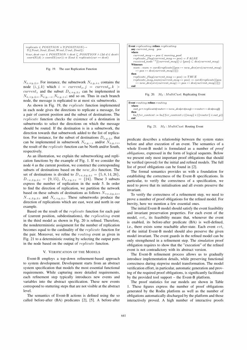
replicate ∈ POSITION × P(POSITION)→P({Nout, Sout, Eout, Wout, Uout, Dout})∀cur, dest·cur ∈ POSITION ∧ dest ⊆ POSITION ∧ (∃d·d ∈ dest∧coordX(d) > coordX(cur))⇒ Eout ∈ replicate(cur �→ dest)
Fig. 19. The east Replication Function
Nx,+y,±z . For instance, the subnetwork Nx,y,+z contains thenode (i, j, k) which i = currentx, j = currenty, k >currentz and the subset Dx,+y,±z can be implemented inNx,+y,±z, Nx,y,−z, Nx,y,+z; and so on. Thus in each branchnode, the message is replicated to at most six subnetworks.
As shown in Fig. 19, the replicate function implementedin each node gives the directions to replicate a message, fora pair of current position and the subset of destinations. Thereplicate function checks the existence of a destination insubnetworks to select the directions on which the messageshould be routed. If the destination is in a subnetwork, thedirection towards that subnetwork added to the list of replica-tion. For instance, for the subset of destinations Dx,y,±z thatcan be implemented in subnetwork Nx,y,−z and/or Nx,y,+z ,the result of the replicate function can be North and/or South,respectively.
As an illustration, we explain the subnetworking and repli-cation functions by the example of Fig. 1. If we consider thenode 4 as the current position, we construct the correspondingsubsets of destinations based on the new des function. Theset of destinations is divided to D+x,±y,±z = {5, 8, 14, 26},D−x,±y,±z = {9, 15}, Dx,+y,+z = {24}. These 3 subsetsexpress the number of replication in the node 5. In orderto find the direction of replication, we partition the networkbased on these subsets of destinations as follows N+x,±y,±z ,N−x,±y,±z and Nx,+y,±z . These subnetworks produce thedirection of replications which are east, west and north in ourexample.
Based on the result of the replicate function for each pairof (current position, subdestinations), the replicating eventin the third model as shown in Fig. 20 is refined. Therefore,the nondeterministic assignment for the number of replicationbecomes equal to the cardinality of the replicate function forthe pair. Moreover, we refine the routing event as given inFig. 21 to a deterministic routing by selecting the output portsin the node based on the output of replicate function.
V. VERIFICATION OF THE MODELS
Event-B employs a top-down refinement-based approachto system development. Development starts from an abstractsystem specification that models the most essential functionalrequirements. While capturing more detailed requirements,each refinement step typically introduces new events andvariables into the abstract specification. These new eventscorrespond to stuttering steps that are not visible at the abstractlevel.
The semantics of Event-B actions is defined using the socalled before-after (BA) predicates [2], [5]. A before-after
Event replicating refines replicatingany current msg poswhere
current msg �→ pos ∈ moving poolreplicate flag(current msg �→ pos) = FALSEreceived node−1[{current msg}] ∪ {pos} ⊂ des(current msg)
Witnessesnum : num = card(replicate[{pos �→ new des(src(current msg)�→ pos �→ des(current msg))}])
thenreplicate flag(current msg �→ pos) := TRUEreplicate msg num(current msg �→ pos) := card(replicate[{pos�→ new des(src(current msg) �→ pos �→ des(current msg))}])
end
Fig. 20. M3 : MultiCast: Replicating Event
Event routing refines routingwhere
out p=replicate(router �→new des(src(msg) �→router �→des(msg)))then
buffer content := buffer content∪ ({msg}×({router}×out p))end
Fig. 21. M3 : MultiCast: Routing Event
predicate describes a relationship between the system statesbefore and after execution of an event. The semantics of awhole Event-B model is formulated as a number of proofobligations, expressed in the form of logical sequents. Belowwe present only most important proof obligations that shouldbe verified (proved) for the initial and refined models. The fulllist of proof obligations can be found in [2].
The formal semantics provides us with a foundation forestablishing the correctness of the Event-B specifications. Inparticular, to verify the correctness of a specification, weneed to prove that its initialisation and all events preserve theinvariant.
To verify the correctness of a refinement step, we need toprove a number of proof obligations for the refined model. Forbrevity, here we mention a few essential ones.
The initial Event-B model should satisfy the event feasibilityand invariant preservation properties. For each event of themodel, evti, its feasibility means that, whenever the eventis enabled, its before-after predicate (BA) is well-defined,i.e., there exists some reachable after-state. Each event evtiof the initial Event-B model should also preserve the givenmodel invariant. The event guards in the refined model can beonly strengthened in a refinement step. The simulation proofobligation requires to show that the ”execution” of the refinedevent is not contradictory with its abstract version.
The Event-B refinement process allows us to graduallyintroduce implementation details, while preserving functionalcorrectness during stepwise model transformation. The modelverification effort, in particular, automatic generation and prov-ing of the required proof obligations, is significantly facilitatedby the provided tool support – the Event-B platform.
The proof statistics for our models are shown in Table1. These figures express the number of proof obligationsgenerated by the Rodin platform as well as the number ofobligations automatically discharged by the platform and thoseinteractively proved. A high number of interactive proofs
641641

were due to reasoning about set comprehension and unions,not currently supported automatically in Rodin. In addition,the interactive proving often involved manually suggestingvalues to discharging various properties containing logicaldisjunctions or existential quantifiers. Extra proving was dueto the fact that currently, we cannot create proof scripts andreuse them whenever needed in RODIN. Thus, in some caseswe had to manually repeat very similar or almost identicalproofs.
TABLE IPROOF STATISTICS
Model Number of Proof Automatically InteractivelyObligations Discharged Discharged
Context 21 6(28%) 15(72%)Multicast XYZ Context 14 7(50%) 7(50%)M0 Model 121 77(64%) 44(36%)M1 Model 36 14(39%) 22(61%)M2 Model 34 8(24%) 26(76%)Unicast XYZ Model 2 2(100%) 0(0%)Multicast XYZ Model 5 2(40%) 3(60%)
Total 233 116(50%) 117(50%)
We note here two proof-related aspects. First, the interactiveproofs are in a significant proportion rather easy to discharge.Second, the RODIN platform is continuously developing andthus, the number of interactive proofs is very likely to diminishin the near future. This will obviously increase the proofdischarging process.
VI. CONCLUSION
In this paper we have proposed a general model for themulticast communication in 3D NoCs. Our model is a gener-alization of a recently proposed model for unicast communi-cation [12]; we show that the communication model in [12] isa special case or our more general model here. We apply themulticast communication model to develop two variants of theXYZ routing algorithm, one based on the unicast routing andthe other on the tree-based routing. Both algorithms are thusprovably correct.
Our general model for multicast communication can befurther employed for analysis. For instance, we plan to com-pare different communication schemes in terms of efficiencyand developing effort. Thus, we have a general platform forspecifying, developing, and analyzing communication, basedon provably correct modeling.
A side effect of modeling multicast communication is thatwe can employ it for modelling broadcast communication aswell, by setting the destination set of a message to includeall the network nodes in the ROUTER set. It remains to beseen if other broadcast methods, for instance flooding, can begenerated directly from our general model or not.
REFERENCES[1] J. R. Abrial, A system development process with Event-B and the Rodin
platform, ICFEM2007. LNCS, vol. 4789, pp. 1-3. Springer, 2007.[2] J. R. Abrial, Modeling in Event-B: System and Software Design, Cam-
bridge University Press, 2010.[3] L.Tsiopoulos, M. Walden, Formal Development of NoC Systems in B,
In Nordic Journal of Computing, pp. 127-145, 2006.
[4] J. R. Abrial. The B-Book: Assigning Programs to Meanings. CambridgeUniversity Press, 1996.
[5] Rigorous Open Development Environment for Complex Systems(RODIN). Deliverable D7, Event-B Language, online athttp://rodin.cs.ncl.ac.uk/.
[6] RODIN Tool Platform, http://www.event-b.org/platform.html.[7] J. R. Abrial, D. Cansell, D. Mery, Refinement and Reachability in Even-
B. In 4th International Conference of B and Z Users, pp. 129-148, 2005.
[8] J. R. Abrial, S. Hallerstede, Refinement, Decomposition and Instantiationof Discrete Models: Application to Event-B, In Fundamenta Informaticae,pp. 1-28, 2007.
[9] R. J. Back and K. Sere. Stepwise Refinement of Action Systems. In J.L. A. van de Snepscheut (ed), Proceedings of MPC’89 – Mathematics ofProgram Construction, pp. 115-138, 1989.
[10] S. Katz, A Superimposition Control Construct for Distributed Systems.In ACM Transactions on Programming Languages and Systems, pp. 337-356, 1993.
[11] R. J. Back and K. Sere. Superposition Refinement of Reactive Systems.In Formal Aspects of Computing, Vol. 8, No. 3, pp. 324-346, Springer-Verlag, 1996.
[12] M. Kamali, L. Petre, K. Sere and M. Daneshtalab, Refinement-BasedModeling of 3D NoCs, In 4th IPM International Conferenece on Funda-mentals of Software Engineering (FSEN11), to apear 2011.
[13] B. S. Feero and P. Pande, Networks-on-Chip in a Three-DimensionalEnvironment: A Performance Evaluation. In IEEE Transactions on Com-puters, pp. 32-45, 2009.
[14] I. Loi and L. Benini, An Efficient Distributed Memory Interface forMany-Core Platform with 3D Stacked DRAM. In Proc. of the DATEConference, Germany, pp. 99-104, 2010.
[15] D. Park et al., Mira, A Multi-Layered On-Chip Interconnect RouterArchitecture, In ISCA 2008, pp. 251-261, 2008.
[16] A. Nayebi , S. Meraji , A. Shamaei , H. Sarbazi-azad, XMulator: Alistener-Based Integrated Simulation Platform for Interconnection Net-works, In Asia International Conference on Modeling and Simulation,pp. 128-132, 2007.
[17] M. Palesi, R. Holsmark, S. Kumar, V. Catania, Application SpecificRouting Algorithms for Networks on Chip, In IEEE transactions onParallel and Distributed Systems, pp. 316-330, 2009.
[18] R. Kaivola, R. Ghughal, N. Narasimhan, A. Telfer, J. Whittemore, etal, Replacing Testing with Formal Verification in Intel control sequenceCoreTM i7 Processor Execution Engine Validation, In Computer AidedVerification, pp.414-429, 2009.
[19] J. Harrison, Formal Verification at Intel, In Symposium on Logic inComputer Science, 2003.
[20] R. Gupta, P. L. Guernic, S. K. Skuhla. Formal methods and models forsystem design: a system level perspective. Kluwer Academic Publishers,2004.
[21] W. Liao , P. Hsiung, Creating a Formal Verification Platform forIBM CoreConnect-based SoC, In the 1st International Workshop onAutomasted Technology for Verificatin and Analysis (ATVA2003), pp. 7-18, 2003.
[22] E. A. Carara, F. G. Moraes, Deadlock-Free Multicast Routing Algorithmfor Wormhole-Switched Mesh Networks-on-Chip, in Prof. of ISVLSI,pp.341-346, 2008
[23] M. Daneshtalab, M. Ebrahimi, S. Mohammadi, A. Afzali-Kusha, Lowdistance path-based multicast algorithm in NOCs, in IET Computers andDigital Techniques, Special issue on NoC, Vol. 3, Issue 5, pp. 430-442,Sep 2009.
[24] P. Mohapatra, V. Varavithya, A hardware multicast routing algorithm fortwo-dimensional meshes, in proc. Int. Conf. SPDP, New Orleans, 1996,pp. 198205.
[25] R. V. Boppana, S. C, C.S R, Resource deadlock and performance ofwormhole multicast routing algorithms, IEEE Transactions on Paralleland Distributed Systems, pp. 535-549, 1998.
[26] P. Abad, V. Puente and J. . Gregorio, MRR: Enabling Fully AdaptiveMulticast Routing for CMP Interconnection Networks, High PerformanceComputer Architecture (HPCA), 2009.
642642


Paper VII
CorreComm: A Formal Hierarchical Framework
for Communication Designs
Maryam Kamali, Luigia Petre, Kaisa Sere
and Masoud Daneshtalab
Originally published in: Proceedings of the 2nd IEEE International Con-ference on Networked Embedded Systems for Enterprise Applications - NE-SEA2011, pp. 1-7. IEEE Computer Society, December, 2011.
169


CorreComm: A Formal Hierarchical Framework forCommunication Designs
Maryam Kamali∗†, Luigia Petre∗, Kaisa Sere∗ and Masoud Daneshtalab‡∗Abo Akademi University, Finland
Email: {maryam.kamali,luigia.petre,kaisa.sere}@abo.fi†Turku Centre for Computer Science (TUCS), Finland
‡University of Turku, FinlandEmail: [email protected]
Abstract—The number of communicating components hastremendously increased, both at the chip-level communicationas well as in general networks. This leads to an increasedcomplexity in the design of communication infrastructures. Inorder to rely on such complex communication designs, we needa correspondingly increased verification effort. In this paper wepropose a structured framework named CorreComm to alleviatethe modeling and verifying of communication designs. We de-scribe the correct-by-construction structure of our frameworkand demonstrate its applicability as a communication designpattern, by instantiating it to two specific communication models.
Index Terms—Communication designs; Communication pat-terns; Formal methods; Event-B; Refinement
I. INTRODUCTION
Networks and communication are present nowadays in theeveryday life, in an extremely pervasive manner. The financialsystems, including banking and stock exchanges, the travelingsystems, including booking flights and hotels, the electricgrids administration, the nuclear plants processes, etc - are allexamples of essential components of the society being grad-ually adapted to functioning online, via the internet or othernetworking configurations. At the chip level, the Network-on-Chip (NoC) communication paradigm [1], based on a modularpacket-switching mechanism, can address many of the on-chipcommunication design issues such as performance limitationsof long interconnects and the integration of high numbers ofIntellectual Property (IP) cores on a chip. Multicore chips areembedded in a multitude of systems and appliances, effectivelytransforming the way we use our phones and TVs, the waywe pay for our shopping, the way we travel, and the wayour health is supported, to only name a few applications.The communication designs for this variety of systems hasgradually become more and more complex and more and moreessential for us.
Given the widespread and relevance of communication, itis imperiously necessary to be able to rely on the communi-cation designs, i.e., to be certain of their various properties.Formal methods, with their mathematic proving core, are animportant instrument in ensuring the integrity of software-intensive systems. Traditionally characterized as hard to use,due to the requested mathematical background and the lack ofautomatic tools, nowadays formal methods have matured, to
the point where they are considered in industry when develop-ing software-intensive systems [2]. Examples of the industrialundertaking of formal methods are increasing. The famousline 14 of the driverless Parisian metro [3], developed in 1998using the B-method [4], is the first notable example of a formalmethod-based development, reviewed in [5]. The method usedby Siemens for developing the software controlling the line14 train ensured its correctness in a mathematical mannerthat effectively eliminated the unit testing from the softwarelifecycle. No human resources are now needed to operate thetrains and in addition, the trains are faster, hence fewer areneeded in total.
More recent examples of the Event-B [6] formal method us-age in industry can be seen for instance with Space Systems [7]and SAP [8]. In Event-B, the development of a model iscarried out step by step from an abstract specification to moreconcrete implementations. Using the refinement approach, asystem can be described at different levels of abstraction,and the consistency in and between levels can be provedmathematically.
In this paper we propose a hierarchical framework namedCorreComm for modeling communication designs as well asfor verifying their correct construction. Modeling and verify-ing full communication designs is very complex and time-consuming. In our methodology we propose to model andverify different components of the communication designs in astepwise and hierarchical manner. We ensure the correctnessof these components by developing them via refinement inEvent-B. Moreover, these components can be further refined inorder to model various specific communication design choices.Hence, the contribution of our paper can be summarized asfollows:
• we propose CorreComm, a framework for facilitating thedesign exploration of possible communication infrastruc-tures
• we introduce a methodology for alleviating the verifica-tion effort for communication designs
• we demonstrate the applicability of the methodologyby deriving two specific communication models, namelythe first-in, first-out (FIFO) buffer and the wormholeswitching technique
978-1-4673-0498-6/11/$26.00 ©2011 IEEE

We proceed as follows. In Section II we describe Event-Bto the extent needed in this paper. In Section III we describethe main components of CorreComm and in Section IV wedetail the stepwise construction of CorreComm in Event-B.In Section V we discuss the applicability of CorreComm asa communication design pattern and in Section VI we bringforward the verification techniques employed in this paper.Related work is briefly surveyed in Section VII. We concludethe paper in Section VIII.
II. THE EVENT-B MODELING METHOD
Event-B [6] is a formal method for modeling and reasoningabout distributed systems. The semantics of Event-B is basedon transition systems and before-after predicates. Modeling inEvent-B is based on set theory and first order logic, whilethe key feature of Event-B consists in promoting the correct-by-construction approach based on the refinement concept [9],[10], [11]. This means that a system can be modeled in variousdegrees of detail at different abstraction levels; the modelconsistency of each level can be verified, together with theconsistency of the models in between levels. The refinementapproach promotes the development of a model gradually, bymaking it more precise and detailed in each step. This leads tothe control of complexity as system development is based ona model chain, with each model a refinement of the previousmodels in the chain.
Event-B models are composed of contexts and machines.A context describes the static part of a model, made ofcarrier sets and constants, together with axioms describingthe properties of these. A machine describes the dynamicpart of a model. Machines can contain variables, invariantsand events. The values of the variables v define the stateof a machine. Variables are constrained by invariants I(v)which should be preserved by any changes in the value ofthe variables. The state changes are specified by a number ofevents. Each event is formed of a guard and an action. Theguard G(t, v), where t are the local parameters of the event, isthe necessary condition under which the event may occur. Theaction S(v, t) models how the state variables change when theevent executes. An event may be executed only when its guardholds. The semantics of Event-B actions is defined using theso called before-after (BA) predicates [6], [12]. A before-afterpredicate describes the relationship between the system states,before and after the execution of an event.
A refined model RM usually has more variables than itsabstraction AM . The state of AM is related to the state of theRM by a gluing invariant J(v, w), where v are the variablesof AM and w are the variables of AM . There are severaltypes of refinement, out of which we employ in this papersuperposition refinement and data refinement. Superpositionrefinement [13], [14] corresponds to adding new data and newevents on top of the already existing data and events, but insuch a way that the introduced behavior does not contradict ortake over the abstract machine behavior. Data refinement [15]refers to replacing some (more abstract) variables with someother (more concrete) variables in a manner controlled by the
gluing invariant. Correspondingly, the events dealing with theold variables are replaced by several corresponding events inthe refined machine.
In this paper we describe all the Event-B modeling in theform of simplified explanations and diagrams, due to lack ofspace. However, the discussed models are fully developed andproved in Event-B and will appear as online material in duetime.
III. THE STRUCTURE OF CORRECOMM
In this section we introduce the structure of the CorreCommframework and outline the purpose of each component of theframework.
With CorreComm we propose that a communication de-sign consists of three main components: CommunicationArchitecture, Communication Primitives, andCommunication Properties, as illustrated in Fig. 1.
The Communication Architecture component de-scribes the communicating elements, their relationship to eachother, and various other constructs needed for communi-cation. It consists of two sub-components as illustrated inFig. 1: a Structural Elements sub-component and aRelationships sub-component. Further on, there are threemain types of structural elements involved in communicationdesigns, namely Node, Channel and Buffer. A nodedenotes any type of communicating unit. A channel connectsnodes together. A buffer stores data temporarily in the start andend points of the channels. The behavior of each individual el-ement can be varied from a communication design to another.In other words, the basic functionality of each element can beextended or refined to a specific design scheme. However, thisfoundation is common to all the communication architectures.The relationships between the elements in the network showsthe topology of the architecture.
The communication architecture shows how different el-ements are connected to each other in order to transfermessages. The message transfer methods are described in theCommunication Primitives component of our frame-work. There are four main communication primitives, namelyInjecting, Switching, Routing and Receiving, asillustrated in Fig. 1. Injecting refers to introducing a newmessage in the network. Routing refers to deciding the routethat a message should follow. Switching determines when therouting decisions are made, the setting/resetting of the switchesinside the nodes, and how the messages are transferred insidethe nodes. Receiving is the function that deletes the messageshaving reached their destination from the network.
The Communication Properties component is in-tended for the modeling and verification of the communicationdesign properties, based on the given architecture and primi-tives. The main purpose of formal modeling a communicationdesign is to verify the correctness of communication. A typicalproperty for the functional correctness of communication isthat all the injected messages are received by all their des-tinations. However, other properties can be modeled as well,for instance non-functional properties such as the performance
978-1-4673-0498-6/11/$26.00 ©2011 IEEE

Fig. 1. Communication Scheme
or energy consumption of a given communication design.In this paper we only refer to the functional correctness ofcommunication.
IV. THE STEPWISE CONSTRUCTION OF CORRECOMM INEVENT-B
In this section, we describe the modeling of the proposedstructure of communication designs in Event-B and discussits correctness. The communication architecture describes thestatic part of a communication network, so all its elements arespecified in the context part of the model as sets, constants,and axioms. The communication primitives define the dynamicbehavior of the communication network, therefore are modeledin the machine part of the Event-B model as variables andevents. The communication properties are modeled as a listof invariants in the machine part of the model and verifiedby a list of proof obligations. In the following we outline thisdevelopment.
We model the communication design elements in a stepwisemanner, employing the abstraction and refinement concepts putforward in Section II. For every abstraction level we have acorresponding context, machine, list of invariants, and list ofproof obligations to discharge. The initial model consists ofthe least number of structural elements so that the correctnessproperty is formulated. In the subsequent levels, we graduallyadd the other structural elements in such a way that they donot contradict with the previous models. As we hierarchicallyrefine the architecture, the communication primitives compo-nent is also hierarchically refined. In each abstraction levelwe verify the communication properties, expressed in termsof the (hierarchically-)corresponding architectural elementsand primitives. The stepwise development continues until allthe elements of the communication design are modeled. Theresulted model can then be employed to specify more precisestructural elements as well as specific communication designs.
In Level 1 of abstraction, we consider just a small numberof structural and primitive elements, essentially as few aspossible for expressing relevant invariants. This means thatsome elements are abstracted away from this initial model.More precisely, in Level 1 we model the structural elementNode by defining a set Node that models the elements ofthe communication network. Technically, the set of nodes isa parameter of our model. The relationships between these
nodes, defining the network topology, are modeled with aconstant named Neigh. This constant effectively records thepairs of related nodes. In order to model the functionalcorrectness of the communication, we need to specify that allthe injected messages are received by all their destinations.For this, we model another set, Msg, as a parameter of ourmodeling. A message in the network has a source node and aset of destination nodes, hence any element of Msg is a triple(msgID, src, {des}).
We model the corresponding communication primitives inLevel 1 with variables and events. Thus, in the initial modelwe have four abstract variables: snt pl,mv pl, rcv nd andrcv pl. These variables are enough for modeling (and veri-fying) the functional correctness of the communication. Thesnt pl variable denotes the list of messages which are injectedby a source node to the network. The mv pl variable denotesthe current position of messages still traveling in the network.The rcv nd variable models the instances of messages havingreached destinations. When a message is received to one ofits destinations, a corresponding map is added to the rcv ndrelation. The rcv pl denotes the list of messages which areremoved from the network by all their destinations, i.e., amessage-to-destination map for all of the destinations of thatmessage should be in rcv nd.
The four communication primitives are abstractly modeledin Level 1 by three events: inject msg, travel msg, andreceive msg. The inject msg event handles the injectingprimitive by adding a new message to the snt pl set and themv pl set. The reason for adding the message to mv pl isto launch the message transferring process. The travel msgevent handles both switching and routing primitives in Level1, by modeling the transferring of a message from a node toanother. We thus postpone the modeling of specific routingand switching primitives for the subsequent refinement steps.The receive msg event handles the receiving primitive of thecommunication model in two different situations. Either themessage is received by all its destinations or, there are stillsome destinations that did not receive the message. In theformer case, the message is added to the rcv pl and removedfrom the mv pl. In the latter, the corresponding message-to-destination map is added to rcv nd and the message is notadded to rcv pl because there are still destinations waiting forthe message.
We model the functional correctness of the communication,i.e., that all the injected messages are received by all theirdestinations, with the following invariant:
mv pl = ø ⇔ snt pl = rcv pl
This predicate models the equivalence between no travelingmessage (i.e., all the traveling messages have reached theirdestinations) and the receiving pool of messages containingall the injected messages.
The initial model forms the first hierarchical level, Level1, of our development. Level 1 is a foundation model for thesubsequent refinement steps, where we refine the context part
978-1-4673-0498-6/11/$26.00 ©2011 IEEE

Fig. 2. Communication Scheme in Event-B
of the model to extend the communication architecture andrefine the machine part of the model to refine the communi-cation primitives. The mapping between the communicationdesign to Event-B is summarized in Fig. 2.
In Level 2, we extend the initial context to model theChannel structural element. We specify the set Channelthat (physically) connects neighbor nodes to each other. Inother words, for any pair in the Neigh relation, we modela channel that connects the pair by modeling two rela-tions: start ch nd : Node ↔ Channel and end ch nd :Channel ↔ Node. The composition of these two relations isequal to Neigh relation. Now, we refine the communicationprimitive component to specify the transferring of messagesthrough the channels. In this level of hierarchy, we use the datarefinement technique. In the initial model, the mv pl relationdenotes the current position of messages in the network. Inorder to represent the existence of messages in both nodes andchannels, in the second model we replace the mv pl variablewith two variables: mv nd and mv ch. The mv nd variabledenotes the current position of those messages that are in nodesand the mv ch variable denotes the current position of thosemessages that are in channels. In fact, the union of messagesin these two relations is equal to those messages in mv pl.
mv pl = mv nd ∪ (mv ch; start ch nd)
As a consequence of this substitution, the events thatrepresent the communication primitive component are up-dated, so that all the connections to mv pl are substituted
either by mv nd or by mv ch. In addition, we refine thetravel msg event by splitting it into two events: travel to chand travel to nd. The travel to ch event models the trans-ferring of a message from a node to a channel and thetravel to nd models the transferring of a message from achannel to a node at the end of the channel. This data refine-ment comes with a list of proof obligations that express thecorrectness of the replacement. These obligations guaranteethat the second model preserves the communication propertiescomponent.
In the third model (Level 3) we add the Buffer structuralelement by modeling a parameter set Buf and a constantBuf size. We refine accordingly the dynamic part of themodel. Intuitively, at the start and at the end points of anychannel, we now model a buffer of size Buf size that storesthe messages. Each node consists of a number of input andoutput buffers depending on its input and output channels.Any message in a node settles in either an input buffer of thenode or an output buffer of the node. Therefore, the mv ndvariable is replaced by the buf in and buf out variables, viadata refinement. The buf in variable denotes the content ofthe input buffers of nodes and the buf out variable denotesthe content of the output buffers for nodes.
At this level of abstraction, we refine the travel to ndevent in the second model to the travel ch ibuf event. Thetravel ch ibuf event models the receipt of a message from achannel, provided that the buffer at the end of the channel hasspace to add a new message. This event releases the channeland adds the message to the input buffer of the node corre-sponding to the end of the channel. The travel to ch eventthat models transferring of a message from a node to someneighbors is refined to the travel obuf ch event. When thereis a message in an output buffer and the channel correspondingto the buffer is free, the travel obuf ch removes the messagefrom the output buffer and adds it to the channel. The newlyintroduced travel ibuf obuf event models the transfer ofa message from an input buffer of a node to a number ofoutput buffers of the node in a nondeterministic manner. Thisnondeterminism can be refined to specific routing techniquesin subsequent refinements.
In this refinement step we establish the connection betweenabstract variables and the more concrete variables by thefollowing gluing invariant:
∀msg, n.msg �→ n ∈ mv nd ⇔(∃ch.(ch ∈ start ch nd˜([{ch}]) ∧msg ∈ buf in(ch))∨(ch ∈ end ch nd˜([{ch}]) ∧msg ∈ buf out(ch)))
This invariant guarantees that all the mappings in themv nd relation in the abstract model are in either buf inor buf out. When we prove that the invariant preserve by allthe events in the machine, we guarantee the communicationcorrectness.
The third level of hierarchy presents the foundation frame-work of the communication design. The way which is devel-oped shows how we can use the framework and the refinementmethod to model and verify a specific communication designs.
978-1-4673-0498-6/11/$26.00 ©2011 IEEE
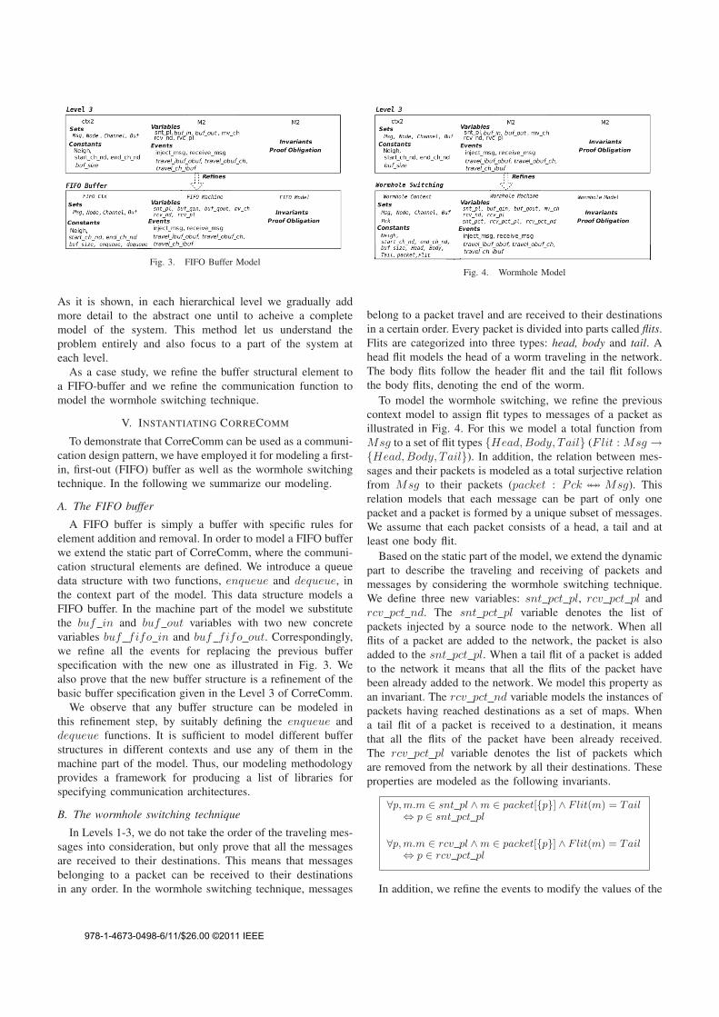
Fig. 3. FIFO Buffer Model
As it is shown, in each hierarchical level we gradually addmore detail to the abstract one until to acheive a completemodel of the system. This method let us understand theproblem entirely and also focus to a part of the system ateach level.
As a case study, we refine the buffer structural element toa FIFO-buffer and we refine the communication function tomodel the wormhole switching technique.
V. INSTANTIATING CORRECOMM
To demonstrate that CorreComm can be used as a communi-cation design pattern, we have employed it for modeling a first-in, first-out (FIFO) buffer as well as the wormhole switchingtechnique. In the following we summarize our modeling.
A. The FIFO buffer
A FIFO buffer is simply a buffer with specific rules forelement addition and removal. In order to model a FIFO bufferwe extend the static part of CorreComm, where the communi-cation structural elements are defined. We introduce a queuedata structure with two functions, enqueue and dequeue, inthe context part of the model. This data structure models aFIFO buffer. In the machine part of the model we substitutethe buf in and buf out variables with two new concretevariables buf fifo in and buf fifo out. Correspondingly,we refine all the events for replacing the previous bufferspecification with the new one as illustrated in Fig. 3. Wealso prove that the new buffer structure is a refinement of thebasic buffer specification given in the Level 3 of CorreComm.
We observe that any buffer structure can be modeled inthis refinement step, by suitably defining the enqueue anddequeue functions. It is sufficient to model different bufferstructures in different contexts and use any of them in themachine part of the model. Thus, our modeling methodologyprovides a framework for producing a list of libraries forspecifying communication architectures.
B. The wormhole switching technique
In Levels 1-3, we do not take the order of the traveling mes-sages into consideration, but only prove that all the messagesare received to their destinations. This means that messagesbelonging to a packet can be received to their destinationsin any order. In the wormhole switching technique, messages
Fig. 4. Wormhole Model
belong to a packet travel and are received to their destinationsin a certain order. Every packet is divided into parts called flits.Flits are categorized into three types: head, body and tail. Ahead flit models the head of a worm traveling in the network.The body flits follow the header flit and the tail flit followsthe body flits, denoting the end of the worm.
To model the wormhole switching, we refine the previouscontext model to assign flit types to messages of a packet asillustrated in Fig. 4. For this we model a total function fromMsg to a set of flit types {Head, Body, Tail} (Flit : Msg →{Head, Body, Tail}). In addition, the relation between mes-sages and their packets is modeled as a total surjective relationfrom Msg to their packets (packet : Pck ↔↔ Msg). Thisrelation models that each message can be part of only onepacket and a packet is formed by a unique subset of messages.We assume that each packet consists of a head, a tail and atleast one body flit.
Based on the static part of the model, we extend the dynamicpart to describe the traveling and receiving of packets andmessages by considering the wormhole switching technique.We define three new variables: snt pct pl, rcv pct pl andrcv pct nd. The snt pct pl variable denotes the list ofpackets injected by a source node to the network. When allflits of a packet are added to the network, the packet is alsoadded to the snt pct pl. When a tail flit of a packet is addedto the network it means that all the flits of the packet havebeen already added to the network. We model this property asan invariant. The rcv pct nd variable models the instances ofpackets having reached destinations as a set of maps. Whena tail flit of a packet is received to a destination, it meansthat all the flits of the packet have been already received.The rcv pct pl variable denotes the list of packets whichare removed from the network by all their destinations. Theseproperties are modeled as the following invariants.
∀p, m.m ∈ snt pl ∧m ∈ packet[{p}] ∧ Flit(m) = Tail⇔ p ∈ snt pct pl
∀p, m.m ∈ rcv pl ∧m ∈ packet[{p}] ∧ Flit(m) = Tail⇔ p ∈ rcv pct pl
In addition, we refine the events to modify the values of the
978-1-4673-0498-6/11/$26.00 ©2011 IEEE

Fig. 5. Formal Development in Event-B
new variables. Thus, we refine the inject msg event to add apacket to snt pct pl if the current injected message is a tail.We also add new constraints in the guard of the event to modelthe order of the injected messages to the network. The guardsand actions of other events are similarly extended to model thetraveling and receiving of packets based on the flow controldefined by the wormhole switching technique. More precisely,the head of a packet is always traveling in the network withthe following subsequent flits and there are no flits from otherpackets between them. These properties are given as a listof invariants in the model to guarantee the correctness of themodel.
VI. ON THE VERIFICATION OF CORRECOMM
The main purpose of formal modeling consists in reasoningabout and finding out the design problems. In the Event-Bframework reasoning is supported by formal proof. With eachformal model we generate a number of proof obligations thatestablish the properties of our model. The proof obligations,described in the form of logical sequents, express the seman-tics of a whole Event-B model.
In this paper, we rely on the Rodin Platform [16], [12]tool where proof obligations are generated automatically andproven either automatically or interactively. The Rodin plat-form [12], which is based on Eclipse, facilitates modeling inthe Event-B language. In addition to providing a user interfacefor editing Event-B models, it generates proof obligationsregarding the model on the fly, updating these every time themodel is saved, discharges some of these proof obligationsautomatically and allows the user to interactively dischargethe rest.
By discharging the proof obligations we guarantee thecorrectness of our model. However, when we fail to dischargesome proof obligations, we modify the model and again tryto discharge the proof obligations of the modified model.The modification process continues until all proof obligationsare discharged. In the Event-B formalism, discharging proofobligations thus provides a means to deeply understand andreason about our designs. Constructing a correct model of asystem in Event-B is a cycle of modeling and proving proofobligations in different level of abstractions as shown in Fig. 5.
To exemplify the cycle of modeling and proving, we con-sider one of the behavioral properties of Event-B models,namely invariant preservation. This means that we need to
verify if invariants hold whenever variables change theirvalues via execution of events. While modeling CorreComm,we observed that invariant preservation properties for thereceive msg in the initial model (Level 1) were not automati-cally discharged. By interactive discharging we found a failurein the guard of the event. In the receive msg event, when amessage is received to all its destinations, it is removed fromthe mv pl variable and added to the rcv pl variable; however,when it is not received to all its destinations, no update is donefor the mv pl and rcv pl variables. In the faulty event, we hadconsidered both possible actions while only one of the aboveconditions had been included in the guard. Upon modifyingthe guard of event, we finally could discharge the invariantpreservation property for the receive msg event.
The summary of discharged proof obligations in the finalversion of CorreComm is displayed in Table 1.
TABLE IPROOF STATISTICS
Model Number of Proof Automatically InteractivelyObligations Discharged Discharged
Level1 Context 2 2(100%) 0(0%)Level2 Context 1 1(100%) 0(0%)Level3 Context 0 0(0%) 0(0%)FIFO Context 15 15(100%) 0(0%)Wormhole Context 2 2(100%) 0(0%)Level1 Machine 39 32(82%) 7(18%)Level2 Machine 67 47(70%) 20(30%)Level3 Machine 120 80(67%) 40(33%)FIFO Machine 52 42(81%) 10(19%)Wormhole Machine 138 95(69%) 43(31%)
Total 436 316(72%) 120(28%)
VII. RELATED WORK
Formal methods have been used before for modeling andverifying communication designs at different levels of ab-straction and in different application domains. For instance,in [17], [18] specific communication protocols at the networklayer are modeled and verified independently of the underlyinginfrastructure. In [19], the authors specify and verify thecommunication correctness of the network infrastructure in asystem-level model.
In [20], a framework for designing the communicationnetwork is proposed. Authors present a model for communi-cation synthesis. The model consists of quantities to measurethe performance of a communication component, compositionrules to handle how to build composite components, andcommunication structures to capture the behavior of compositecomponents. In addition, in [21], a modeling framework forcommunication architectures is proposed. The authors presentan application-driven platform for object-oriented modelingof the communication architectures. They introduce a specifichierarchical class library that is used to develop new commu-nication architectures. However, neither [20] nor [21] proposeany verification methods for their communication designs.
Summarizing, there are a number of informal platformsfor the modeling and evaluation of communication designs.
978-1-4673-0498-6/11/$26.00 ©2011 IEEE
Besides, there are mature formal techniques that could beemployed for modeling, verifying, and reasoning about thecommunication designs. However, the formal techniques havenot been applied in the platform level and instead, the majorityof existing formal approaches focus on particular networkingand communication aspects. Our main contribution in thispaper is to introduce CorreComm as a formal hierarchicalframework for modeling and verifying communication designsin order to bridge this gap. For instance, in [22], [23], [24],formal models are introduced to study unicast and multicastcommunication at the chip level as well as to study recoverymechanisms in wireless sensor-actor networks, respectively.With CorreCom, we establish a base communication design,out of which the formal models mentioned above could bederived via refinement in a correct-by-construction manner.
VIII. CONCLUSIONS
In this paper we propose CorreComm, a formal hierarchicalframework for modeling and verifying communication de-signs. CorreComm is developed stepwise based on the Event-B formal method, so that we are sure of its consistency.We have also demonstrated the value of CorreComm asa communication design pattern, in that in can be reused,extended, and refined whenever a communication design needsto be elaborated. With CorreComm we thus avoid errors inthe early stages of elaborating communication designs. Also,when extending CorreComm, one can detect errors in the earlystages of construction, due to the interactive style of modelingand proving in Event-B via the Rodin platform.
CorreComm can be used to construct a library of verifiedcomponents to be employed for the verification of specificcommunication designs. We plan to expand the library of veri-fied components by continuing to model various switching androuting techniques. In addition, we plan to focus on modelingpower consumption issues as communication properties and,in general, to explore the quantitative analysis of the com-munication designs within our formal hierarchical framework.This can easily be seen as extending the CommunicationProperties component of CorreComm. This would allowus to evaluate different parameters of the communicationdesigns and, as a consequence, come up with optimal solutionsfor them.
REFERENCES
[1] M. Daneshtalab, M. Ebrahimi, P. Liljeberg, Juha Plosila, and H. Ten-hunen, A Low-Latency and Memory-Efficient On-chip Network, Inproceedings of 4th IEEE/ACM International Symposium on Network-on-Chip (NOCS), pp. 99-106, May 2010.
[2] J. Woodcock, P. G. Larsen, J. Bicarregui, and J. Fitzgerald. FormalMethods: Practice and Experience. In ACM Computing Surveys, Vol. 41,Issue 4, pp. 1-36, 2009.
[3] D. Craigen, S. Gerhart and T.Ralson, Case Study: Paris Metro SignalingSystem, In the Proceedings of IEEE Software, pp. 32-35, 1994.
[4] J. R. Abrial. The B-Book: Assigning Programs to Meanings. CambridgeUniversity Press, 1996.
[5] T. Lecomte. Applying a Formal Method in Industry: A 15-Year Trajectory.In M. Alpuente, B. Cook and C. Joubert (Eds), Proceedings of the FormalMethods for Industrial Critical Systems, FMICS 2009. Lecture Notes inComputer Science, Vol. 5825, pp. 26-34, Springer-Verlag, 2009.
[6] J. R. Abrial, Modeling in Event-B: System and Software Design, Cam-bridge University Press, 2010.
[7] A. S. Fathabadi, A. Rezazadeh, and M. Butler. Applying Atomicityand Model Decomposition to a Space Craft System in Event-B. In:Proceedings of the THIRD NASA FORMAL METHODS SYMPOSIUM,Lecture Notes in Computer Science, Vol. 6671, pp. 328-342, 2011.
[8] J. Bryans and W. Wei. Formal Analysis of BPMN Models Using Event-B. In the S. Kowalewski and M. Roveri (Eds.), Proceedings of the15th International Workshop on Formal Methods for Industrial CriticalSystems, FMICS 2010. Lecture Notes in Computer Science, Vol. 6371,pp. 33-49, Springer-Verlag, 2010.
[9] R. J. Back and J von Wright. Refinement Calculus: A Systematic Intro-duction. Springer-Verlag, 1998.
[10] J. R. Abrial, D. Cansell, D. Mery, Refinement and Reachability in Even-B. In 4th International Conference of B and Z Users, pp. 129-148, 2005.
[11] J. R. Abrial, S. Hallerstede, Refinement, Decomposition and Instantiationof Discrete Models: Application to Event-B, In Fundamenta Informaticae,pp. 1-28, 2007.
[12] Rigorous Open Development Environment for ComplexSystems (RODIN). Deliverable D7, Event-B Language, online athttp://rodin.cs.ncl.ac.uk/.
[13] S. Katz, A Superimposition Control Construct for Distributed Systems.In ACM Transactions on Programming Languages and Systems, pp. 337-356, 1993.
[14] R. J. Back and K. Sere. Superposition Refinement of Reactive Systems.In Formal Aspects of Computing, Vol. 8, No. 3, pp. 324-346, Springer-Verlag, 1996.
[15] R. J. Back and K. Sere. Stepwise Refinement of Action Systems. In J.L. A. van de Snepscheut (ed), Proceedings of MPC’89 – Mathematics ofProgram Construction, pp. 115-138, 1989.
[16] RODIN Tool Platform, http://www.event-b.org/platform.html.[17] D. Borrione, A. Helmy, L. Pierre, and 1. Schmaltz. A Formal Approach
to the Verification of Networks on Chip. EURASIP Journal on EmbeddedSystems, 2009(548324):1-14, February 2009.
[18] G. Salaun, W. Serwe, Y. Thonnart, and P. Vivet. Formal Verificationof CHP Specifications with CADP Illustration on an AsynchronousNetwork-on-Chip. In Proceedings of International Symposium on Asyn-chronous Circuits and Systems, pages 73-82. IEEE Computer SocietyPress, March 2007.
[19] Y. Chen, W. SU, P. Hsiung, Y. Lan, Y. Hu, and S. Chen, Formal Model-ing and Verification for Network-on-Chip, In Proceeding of InternationalConference on Green Circuits and Systems (ICGCS), pp. 299-304, 2010.
[20] A. Pinto, A. Sangiovanni-Vincentelli and L. P. Carloni, COSI: AFramework for the Design of Interconnection Networks, Design and Testof Computers, IEEE, Vol. 25 Issue:5, pp. 402-415, 2008.
[21] X. Zhu and Sharad Malik, A hierarchical modeling framework foron-chip communication architectures of multiprocessing SoCs, ACMTransactions on Design Automation of Electronic Systems (TODAES),Vol. 12 Issue 1, 2007.
[22] M. Kamali, L. Petre, K. Sere and M. Daneshtalab, Refinement-BasedModeling of 3D NoCs, In 4th IPM International Conferenece on Funda-mentals of Software Engineering (FSEN11), to apear 2011.
[23] M. Kamali, L. Petre, K. Sere, M. Daneshtalab, Formal Modelingof Multicast Communication in 3D NoCs, In the 14th EUROMICROConference on Digital System Design (DSD), appear 2011.
[24] M. Kamali, L. Laibinis, L. Petre, K. Sere, Self-Recovering Sensor-Actor Networks, In proceedings of 9th International Workshop on theFoundations of Coordination Languages and Software Architectures,FOCLASA2010, Sep 2010.
978-1-4673-0498-6/11/$26.00 ©2011 IEEE

Paper VIII
NetCorre: A Hierarchical Framework and Theory
for Network Design
Maryam Kamali, Luigia Petre and Kaisa Sere
Submitted to Science of Computer Programming
179


NetCorre: A Hierarchical Framework and Theory for
Network Design
Maryam Kamalia,b, Luigia Petrea, Kaisa Serea
aDepartment of Information Technologies, Abo Akademi University, Turku, FinlandbTurku Centre for Computer Science (TUCS), Turku, Finland
Abstract
Design decisions made at the algorithm level affect the implementation sig-nificantly. In this paper, we introduce a formal framework for high-levelanalysis of network design in which both design aspects of algorithm andarchitecture are integrated. We hierarchically develop the framework modelrelying on the formal design technique of refinement. In addition, we ex-tract the common features of networks as a library of design rules that arereusable and extendable for modelling and analysing different network de-signs. We elaborate our framework model within the Event-B formalism,using the Rodin platform - an integrated development framework for Event-B; in particular, for modelling the library of design rules, we employ thenovel theory extension mechanism of Event-B and the corresponding plug-inof the Rodin platform.
Keywords: Algorithm-architecture network design; Formal hierarchicalframework; Refinement; Event-B; RODIN Tool
1. Introduction
Design decisions made at the algorithm level affect the implementationsignificantly. Sometimes it is not even possible to apply some algorithmsto some network architectures, and even when this is possible, many time-consuming optimization techniques might still be needed. It is thus impor-tant to be able to analyse the trade-offs of various algorithm-architecturealternatives at higher levels, before investing time and effort in exploringthem at lower levels. For this, both design aspects of algorithm and archi-tecture need to be integrated in a framework for high-level analysis, to allowfor a detailed assessment of implementation parameters.
Preprint submitted to Science of Computer Programming April 18, 2013
Some integrated design frameworks have already proven successful. Adesign exploration methodology is developed in [17] for wireless communi-cations. The author adapts a top-down approach to design optimizationwith a bottom-up module-based approach for implementation estimates. Adesign platform for algorithm-architecture design exploration for efficient im-plementation of multimedia algorithms is proposed in [16]: a pure softwarespecification is gradually transformed into a mixed software and hardwareimplementation.
However, even if the algorithm and the architecture are integrated in thesemethodologies, a significant number of errors as well as undesirable behaviourhave been identified. This strongly motivates the need for checking the in-tegrity of the proposed network designs. An increasingly viable approachfor facilitating the design of correct systems is provided by formal methods.Formal methods are dedicated to the problem of system validation, beingable affect the entire lifecycle of system development from specification toimplementation. System validation ensures that a system satisfies its designspecification and can be performed via testing, simulation, and verification.Verification consists of logical reasoning on the system specification and thuscan detect and avoid possible design errors before system implementation.Validation performed via testing and simulation is limited to the test cases,while verification allows the consideration of all system behaviours.
Therefore, it is clear that formal specification and verification of networkdesigns would increase their reliability and lower their implementation cost.This is mainly due to error detection in the early stages of design. However,using formalisms has some challenges, such as unambiguously formulatingproperties of algorithms and architectures as well as proving them. Con-siderable amounts of expressiveness as well as experience typically help inderiving models and their desired properties.
In this context, we aim at proposing a high-level formal framework thatintegrates the algorithm and architecture analysis for network design. More-over, our proposed framework addresses the challenge of applying formalmethods in the early stages of design. In this paper, with network design werefer to the integrated algorithm-architecture approach to networking andwith modelling the framework we refer to the formal specification and verifi-cation of this integrated framework. The two central features of our proposedframework are that (1) it is intended for reuse in designing verified networksand (2) it is hierarchical; the latter feature is instrumental both in developingthe framework and in its intended reuse.
2

The contribution of this paper is twofold. First, we introduce a reusable,hierarchical formal model of this framework that is verified. Second, fromthe hierarchical model we extract a reusable network theory, also pre-proven.The formal model and the theory are together referred to as NetCorre, forcorrect networking. We base our work on the Event-B formal method [3, 1]for system modelling and analysis. The refinement technique of Event-B isfundamental in our approach because it allows to represent a system at dif-ferent abstraction levels and to prove the consistency between these. Event-Bcomes with an associated toolset Rodin, a theorem prover-based environmentwhere proofs about the models are generated automatically and dischargedeither automatically or interactively. Importantly, the Rodin platform hasextension capabilities: one can define new theories consisting of new datatypes, operators on them, etc. These new theories can be proven in Rodinand then reused as original Event-B constructs. Our proposed network the-ory falls exactly within this reuse pattern. Hence, upon defining a reusable,hierarchical formal model for network design, we extract the fundamentalcomponents to be reused and define the NetCorre network theory. In a nut-shell, our contribution in this paper can be summarized as correct networkreuse.
We proceed as follows. In Section 2 we review related approaches ofinformal and formal network design. In Section 3, we introduce the Event-B formal method that we use, together with its extension mechanisms. InSection 4 we outline the hierarchical framework of algorithm-architecturenetwork design. In Section 5, we detail the development of the framework,based on the refinement technique. In Section 6, we put forward our networktheory proposal and then we wrap up in Section 7.
2. Related Work
An algorithm-architecture design methodology for wireless communica-tions is proposed in [17]. Algorithms are evaluated at an early stage basedon extracting critical characteristics. Their mappings to various architec-tures are then identified in order to improve implementation efficiency. Thepurpose of the proposed methodology in [17] is to optimize the high-leveldesign by analysing design trade-offs.
Another approach for exploring an integrated algorithm and architecturedesign is presented in [16]. A platform is proposed to evaluate the efficiencyof multimedia algorithms in hardware implementations. In contrast to these
3

two design approaches where the focus is on the analysis of design efficiency,our goal in this article is to introduce an integrated algorithm-architecturedesign framework that guarantees the correctness of the integrated design inthe early stages of the lifecycle.
A hierarchical modelling framework for communication architectures ofmultiprocessing SoCs is proposed in [22]. A hierarchical class library is usedto develop communication architectures with incremental effort by adaptingobject-oriented analysis and design methods. The hierarchical approach ofevaluating communication architectures in the proposed framework of [22]is similar to ours. However, it concentrates only on design exploration ofnetwork architectures, without considering network algorithms.
There is a large number of successful approaches that apply the refine-ment technique in producing a correct model of a system under development.Action Systems [8] - a design methodology based on refinement- is used in [19]to propose a formal framework for the design of asynchronous pipelined mi-croprocessors. Another design methodology is proposed in [10] to integratethe Event-B formal method into the SoC design. The role of refinement inSoC development is demonstrated by specifying the system requirements anddeveloping models of the system gradually, while the consistency of the vari-ous models is preserved. Using the refinement technique to produce a correcthigh-level design of a system in [10, 19] is similar to our design methodology.
The Event-B formal method has been widely employed for formal develop-ment and analysis of different network protocols. An algorithm for networktopology discovery [11] is modelled and verified in Event-B. Stepwise andevent-based approaches for modelling and analysing dynamic network pro-tocols are proposed in [7, 6, 12]. A correct-by-construction development of aNoC model is proposed in [15, 14]. In this paper we employ the same formalmethod (i.e., Event-B) in order to develop system models. However, while inthe above articles the focus is on modelling and analysing particular networkalgorithms, hence we introduce a framework for modelling network designs,with an approach integrating algorithm and architecture analysis.
3. Event-B
In this section we shortly introduce Event-B as well as an extension mech-anism in Event-B that we employ in this paper. Event-B [3] is a formalmethod devised for modelling and reasoning about parallel, distributed andreactive systems. Event-B comes with tool support in the form of the Rodin
4

Machine MVariables vInvariants IEventsInitevt1· · ·evtN
Sees−−−→Context CCarrier Sets dConstants cAxioms A
Figure 1: A machine M and a context C in Event-B
platform [2, 21, 20, 4], which provides automated support for modelling andverification by theorem proving.
3.1. Event-B Syntax and Semantics
Event-B Syntax.. In Event-B, the notion of a machine [20] operating onan abstract state is used to specify a system. The state models the problemdomain of the system via a collection of variables and is modified by definedoperations on this state. Thus, it describes the behaviour of the specifiedsystem, also refereed to as the dynamic part. A system model may also havean accompanying component, called context, which contains the static partof the system. Within a context, user-defined sets and constants are declaredand their properties and relationships are defined in a list of model axioms.The general structure of an Event-B model is illustrated in Fig. 1. Therelationship between a machine and its accompanying context is expressed bythe keyword Sees, denoting a structuring technique that allows the machineaccess to the contents of the context.
A machine with the unique name M has a list of state variables v, de-clared in the Variables clause and initialized by the Init event. The variabletypes are declared by the constraining predicates I given in the Invariantsclause. Moreover, the invariant clause may contain other predicates definingproperties that should be preserved over the state of the model. The oper-ations on the variables are given as a set of atomic events specified in theEvents clause. Generally, an event is defined in the following form:
evt = any vl where g then S end,
where the variable list vl contains local variables visible within the event and
5
the guard g represents a state predicate over the state variables v and vl. Theaction S is a statement describing how the event affects the system state andis given in the form of deterministic or non-deterministic assignment over thesystem variable. A deterministic assignment, x := E(x, y), has the standardsyntax and semantics. A non-deterministic assignment is denoted either asx :∈ Set, where Set is a set of values, or as x :| P (x, y, x′), where P is apredicate relating initial values of x, y to some final value x′. As a resultof a non-deterministic assignment, x can get any value belonging to Set oraccording to P .
The occurrence of events represents the observable behaviour of the sys-tem. The event guard defines the conditions under which the action can beexecuted, i.e., when the event is enabled. If several events are enabled at thesame time, any of them can be chosen for execution non-deterministically. Ifnone of the events is enabled then the system deadlocks.
The modelling of a large system in Event-B is based on refinement,i.e., verified modelling in a stepwise manner. Modelling starts from anabstract system specification that models some of the essential functionalrequirements. While capturing more detailed requirements, the model be-comes richer by developing the abstract states and state changes, i.e., intro-ducing new variables and events. This type of model refinement is calledsuperposition refinement. The superposition refinement steps are completewhen all the requirements of the system have been taken into account in themodel. Another kind of refinement is called data refinement and in thiscase abstract variables and events can be replaced with their more concretecounterparts. In a data refinement step, we can remove some variables andadd new ones. Therefore, the invariant of a refined model should define therelationship between the abstract and concrete variables; this type of invari-ants are called gluing invariants. In other words, the state of an abstractmachine is related to the state of a concrete machine by a gluing invariant.In this article we employ both the superposition and data refinement.
The event structure in a refined machine may contain the abstract eventclauses and two other clauses as shown in the following form:
ref evt = refines abs evt any vl where g with w then S end,
where the list of the abstract events, abs evt, that this event refines are enu-merated in the refines clause. The with clause contains the witness of the
6

corresponding abstract event. The witness w is declared in a refining eventfor each disappearing parameter of the abstract event. The witness for pa-rameter a is a predicate P (a). A witness predicate can be either deterministicor non-deterministic. A deterministic witness P (a) is of the form a = E.
Event-B Semantics.. Each construct in Event-B has a well-defined seman-tics. Additionally, machines must satisfy a set of constraints so that ensurethat the specification is internally consistent and also ensure that the be-haviour of a refined machine is consistent with the behaviour of the machinesit refines.
There are three principal constructions, called substitutions, to changethe state of a machine. The semantics of substitution in Event-B is definedusing before-after (BA) predicates. Before-after predicates contain primedand unprimed variables where the primed variables represent the after valueof a variable and the unprimed variables the before value. In general, thesubstitution into a predicate for each of the three constructions takes theform illustrated in Fig. 2
Substitution [Substitution]Rv := E [v := E]Rv :| P ∀v′ · P ⇒ [v := v′]Rv :∈ S ∀v′ · v′ ∈ S ⇒ [v := v′]R
Figure 2: Substitution
where v is a list of variables and E a list of expressions; P is a predicatecontaining both v and v′; v′ represents the value of v after the action.
In an Event-B event, guard is a predicate that identifies a set of pre-stateand action identifies a set of post-states. A before-after predicate relatesthese pre-states and post-states for each event as follows:
BA(evt) = ∃vl. g ∧ BA(S).
The semantics of a whole Event-B model is formulated as a number ofproof obligations, expressed in the form of logical sequent. Below we describeonly the most important proof obligations that should be verified (proved)for the initial and refined models. The full list of proof obligations can befound in [3].
7

Every Event-B model should satisfy the event feasibility and invariantpreservation properties. For each event of the model, evti, its feasibilitymeans that, whenever the event is enabled, its before-after predicate (BA) iswell-defined, i.e., there exists some reachable after-state:
A(d, c), I(d, c, v), gi(d, c, v) ` ∃v′ ·BAi(d, c, v, v′) (FIS)
where A stands for the conjunction of the model axioms, I is the conjunctionof the model invariants, gi is the event guard, d stands for the model sets,c are the model constants, and v, v′ are the variable values before and afterevent execution.
Each event evti of the Event-B model should also preserve the given modelinvariant:
A(d, c), I(d, c, v), gi(d, c, v), BAi(d, c, v, v′) ` I(d, c, v′) (INV)
The invariant preservation proof obligation verifies that each concreteinvariant is preserved by each pair of concrete and abstract events. Sincethe initialisation event has no initial state and guard, its proof obligation issimpler:
A(d, c), BAInit(d, c, v′) ` I(d, c, v′) (INIT)
The formal semantics provides us with a foundation for establishing cor-rectness of Event-B specifications. In particular, to verify correctness of aspecification, we need to prove that its initialisation and all events preservethe given invariant.
Besides, to verify correctness of a refinement step, we need to prove anumber of proof obligations for a refined model. We need to verify thatthe behaviour of a refined machine is consistent with the behaviour of themachine it refines. For brevity, here we show only a few essential ones.
Let us first introduce a shorthand H(d, c, v, w) to stand for the hypothe-ses A(d, c), I(d, c, v), I ′(d, c, v, w), where I, I ′ are respectively the abstractand refined invariants, and v, w are respectively the abstract and concretevariables. Then the feasibility refinement property for an event evti of arefined model can be presented as follows:
H(d, c, v, w), g′i(d, c, w) ` ∃w′. BA′i(d, c, w, w′) (REF FIS)
where g′i is the refined guard and BA′i is a before-after predicate of the refinedevent.
8

The event guards in a refined model can be only strengthened in a refine-ment step:
H(d, c, v, w), g′i(d, c, w) ` gi(d, c, v) (REF GRD)
where gi, g′i are respectively the abstract and concrete guards of the event
evti. The purpose of the guard strengthening proof obligation is to ensurethat the concrete guards in the refining event are stronger than the abstractones.
Finally, the simulation proof obligation (REF SIM) requires to show thatthe ”execution” of a refined event is not contradictory with its abstract ver-sion:
H(d, c, v, w), g′i(d, c, w), BA′i(d, c, w, w′) ` ∃v′.BAi(d, c, v, v′) ∧ I ′(d, c, v′, w′)
(REF SIM)where BAi, BA
′i are respectively the abstract and concrete before-after pred-
icates of the same event evti. The simulation proof obligation ensures thateach action in a concrete event simulates the corresponding abstract action.
The model verification effort and, in particular, automatic generation andproving of the required proof obligations, are significantly facilitated by theprovided tool support – the Rodin platform [1, 21, 20, 4].
Let us note here the quintessential feature of Event-B and its associatedRodin platform. Modelling in Event-B is semantically justified by proofobligations. Every update of a model generates a new set of proof obligationsin the background. It is this interplay between modelling and proving thatsets Event-B apart from other formalisms. Without proving the requiredobligations, we cannot be sure of correctness of a model. The proving effortthus encourages the developer to structure formal model development in sucha way that manageable proof obligations are generated at each step. Thisleads to very abstract initial models so that we can gradually introduce intoa system model various facets of the system. Such a development methodfits well when we have to describe complex algorithms.
The interplay between modelling and proving characteristic of Event-Bprovides suitable formal means to reason about and finding out the designproblems. The perspective of Event-B to modelling matches to our pur-pose of developing a formal framework for network designs because it allowsto construct a correct framework, in each abstract level, by modelling andproving correctness of the model in a cyclic way, as shown in Fig. 3.
9

Figure 3: Formal Development in Event-B
3.2. Event-B Mathematical Extension
Extension Syntax.. We first outline the syntax of the proposed extensionmechanism [5, 9] in Event-B, already implemented in Rodin. In particularwe emphasize the theory component, based on a rule-based prover plug-in;this component allows the declaration of user-defined new predicates, newoperators, new inductive data types and new rewrite rules.
A theory component has a name, a list of global type parameters, and anarbitrary number of definitions and rules for modelling predicates, operators,and inductive data types. The general structure of a theory component isshown in Fig. 4. In the following, we briefly overview the general structureof defining predicates and operators.
theory nametype parameters T1, ..., Tn
{ 〈Predicate Definition〉| 〈Operator Definition〉| 〈DataType Definition〉| 〈Rewrite Rule〉| 〈Inference Rule〉 }
Figure 4: Theory Component
A predicate has a name and can be declared as either infix or prefix witha number of arguments. The condition clause specifies a well-definednesscondition and the argument types are also inferred from the condition. Thedefinition of the new predicate is provided by the definition clause. Thestructure of a predicate definition is shown in Fig. 5.
An operator returns an expression based on a number of expressions.It can be declared as either infix or prefix with a number of arguments.
10

predicate Identifier(prefix or infix)args x1, ..., xn
condition P (x1, ..., xn)definition Q(x1, ..., xn)
Figure 5: Predicate Definition
The condition clause specifies a well-definedness condition and the argumenttypes are also inferred from the condition. The definition clause defines theexpression E (x1, ..., xn). The structure of an operator definition is shown inFig. 6.
operator Identifier(prefix or infix)args x1, ..., xn
condition P (x1, ..., xn)definition E(x1, ..., xn)
Figure 6: Operator Definition
Extension Semantics.. The mathematical extension mechanism of Event-B supports three types of user-defined extensions of the mathematical lan-guage and theory. One type is set-theoretic expressions or predicates exten-sions, the second is the rule library for predicates and operators extensions,and the last is extensions of the set theory itself through the definition ofalgebraic types by using new set constructors. Out of these three extensions,we discuss below the rule library for predicates and expressions which areused in this article to introduce the theory of our framework.
In Event-B, predicates and expressions are introduced as distinct syn-tactic categories. Predicates are defined in terms of basic predicates (>, ⊥,A = B, etc), predicate combinators (¬, ∧, ∨, etc) and quantifiers (∀, ∃).Expressions are defined in terms of constants (0, ø, etc), variables (x, y, etc)and operators (+, ∪, etc). To ensure that mathematical formulas made ofpredicates and expressions are meaningful, they come with type checking.Each expression in a formula is associated with a type which denotes the setof values that the expression can take and it can be in one of the followingforms:
11

� a basic set, that is a predefined set (Z or BOOL) or a carrier set providedby the user;
� a power set of another type α, P(α);
� a cartesian product of two types α and β, α× β
Upon associating a type to each expression the formula is checked by sometype checking rules to prove that it is well-typed. Checking rules enforcethat the operators used can be meaningful. As the type checking is a staticcheck, we cannot always prove that a formula is meaningful. Therefore, forsome operators, some additional dynamic constraints (specified in the well-definedness dynamic checks) are verified. Detecting a meaningless formulais done by disproving some well-definedness lemma. Well-definedness (WD)lemmas are produced by a WD operator that takes a formula as argument.The complete list of the WD operators for basic predicates and expressionsof the Event-B kernel can be found in [18].
In the following, we outline how new predicates and expressions are spec-ified and how their corresponding rules are formed. The corresponding rulesare typing rules and well-definedness rules, as discussed above. A predicatepred is defined in terms of existing predicates and rules for typing the pred-icate arguments x1, . . . , xn as shown in the following table:
Predicate Type rule Definitionpred(x1, . . . , xn) type(x1) = α1 . . . type(xn) = αn P (x1, . . . , xn)
In predicate definition P (x1, . . . , xn), we cannot refer to the newly introducedpredicate pred.
A new operator is defined in terms of an expression along with typing andwell-definedness rules. An operator has a name op and a list of expressionarguments x1, . . . , xn as shown in following table:
Expression Operator Definitionop(x1, . . . , xn) op(x1, . . . , xn) = E(x1, . . . , xn)
In the operator definition, the expression E should not refer to the newlydefined operator op.
The typing rule for the operator op is used by a type checker for expres-sions involving op. The type α for a new operator op is introduced as follows:
12
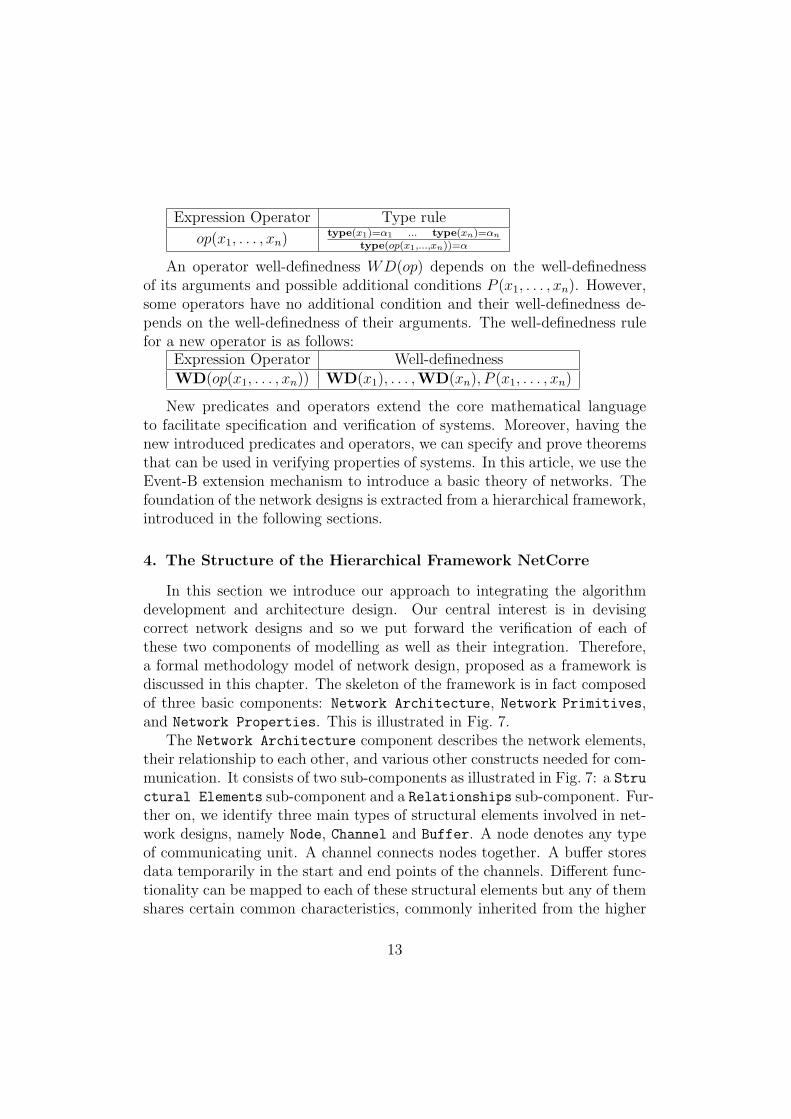
Expression Operator Type rule
op(x1, . . . , xn) type(x1)=α1 ... type(xn)=αn
type(op(x1,...,xn))=α
An operator well-definedness WD(op) depends on the well-definednessof its arguments and possible additional conditions P (x1, . . . , xn). However,some operators have no additional condition and their well-definedness de-pends on the well-definedness of their arguments. The well-definedness rulefor a new operator is as follows:
Expression Operator Well-definednessWD(op(x1, . . . , xn)) WD(x1), . . . ,WD(xn), P (x1, . . . , xn)
New predicates and operators extend the core mathematical languageto facilitate specification and verification of systems. Moreover, having thenew introduced predicates and operators, we can specify and prove theoremsthat can be used in verifying properties of systems. In this article, we use theEvent-B extension mechanism to introduce a basic theory of networks. Thefoundation of the network designs is extracted from a hierarchical framework,introduced in the following sections.
4. The Structure of the Hierarchical Framework NetCorre
In this section we introduce our approach to integrating the algorithmdevelopment and architecture design. Our central interest is in devisingcorrect network designs and so we put forward the verification of each ofthese two components of modelling as well as their integration. Therefore,a formal methodology model of network design, proposed as a framework isdiscussed in this chapter. The skeleton of the framework is in fact composedof three basic components: Network Architecture, Network Primitives,and Network Properties. This is illustrated in Fig. 7.
The Network Architecture component describes the network elements,their relationship to each other, and various other constructs needed for com-munication. It consists of two sub-components as illustrated in Fig. 7: a Stru
ctural Elements sub-component and a Relationships sub-component. Fur-ther on, we identify three main types of structural elements involved in net-work designs, namely Node, Channel and Buffer. A node denotes any typeof communicating unit. A channel connects nodes together. A buffer storesdata temporarily in the start and end points of the channels. Different func-tionality can be mapped to each of these structural elements but any of themshares certain common characteristics, commonly inherited from the higher
13

abstract elements. In this article, the higher abstract structural elements pro-posed in the framework can be reused to develop more concrete elements. Inother words, the common characteristics are introduced and the differencesare encapsulated as block boxes in structural elements. The relationshipsbetween the structural elements in the network shows the topology of thearchitecture.
The Network architecture shows how different elements are connectedto each other in order to transfer messages. The message transfer meth-ods are described in the Network Primitives component of our framework.We identify four main network primitives, namely Injecting, Switching,Routing and Receiving, as illustrated in Fig. 7. Injecting refers to intro-ducing a new message in the network. Routing refers to deciding the routethat a message should follow. Switching determines when the routing deci-sions are made, the setting/resetting of the switches inside the nodes, andhow the messages are transferred inside the nodes. Receiving is the functionthat deletes the messages having reached their destination from the network.The Network Primitives subcomponents proposed in the framework sharecertain common features for algorithm development. In other words, theseare reusable modules that are inherited and refined in the development of anetwork algorithm.
The Network Properties component is intended for the modelling andverification of the network design properties, based on the given architectureand primitives. The aim of this component is to demonstrate that all compo-nents of the framework meet their specifications. Moreover, the interactionand integration satisfies the general correctness properties. A typical prop-erty for the functional correctness of communication is that all the injectedmessages are received by all their destinations. However, other properties canbe modelled as well, for instance non-functional properties such as the net-work performance or energy consumption of a given network design. In thisarticle we only refer to the functional correctness of communication. To verifythe general correctness of the integration in the framework we must analysethe possible interactions of the elements of the Network Architecture andthe Network Primitives to see whether the combined design satisfies thespecification.
Hence, in the proposed framework we concentrate on developing the fun-damental components of a network which are common between all networkdesigns. Therefore, we verify the interactions of these components and weconstruct the framework in such a a way that the correctness of the frame-
14

Figure 7: Network Scheme
work is guaranteed. The components of the framework can be refined bydesigners to construct different network models. However, the designer doesnot need to prove all the properties from the beginning; all the proved prop-erties in the framework can be reused and only the newly added states mustbe verified. We note that using pre-proved components of the framework al-leviates the difficulties of verification and also decreas the design lifecycle. Inthis paper, we additionally provide a library of rules for using the pre-provenfundamental components in order to develop network designs.
5. The stepwise construction of NetCorre in Event-B
In this section, we describe the modelling of the proposed structure ofnetwork designs in Event-B and discuss its correctness. The network ar-chitecture describes the static part of a network, so all its elements andproperties are specified in the context part of the model as sets, constants,and axioms. The network primitives define the dynamic behaviour of thecommunication network, therefore are modelled in the machine part of theEvent-B model as variables and events. The network properties are modelledas a list of invariants in the machine part of the model and verified via proofobligations. In the following we outline this development.
We model the network design elements in a stepwise manner, employingthe abstraction and refinement concepts put forward in Section 3. For everyabstraction level we have a corresponding context, machine, list of invari-ants, and proof obligations to discharge. The initial model consists of the
15
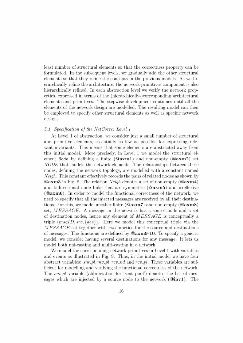
least number of structural elements so that the correctness property can beformulated. In the subsequent levels, we gradually add the other structuralelements so that they refine the concepts in the previous models. As we hi-erarchically refine the architecture, the network primitives component is alsohierarchically refined. In each abstraction level we verify the network prop-erties, expressed in terms of the (hierarchically-)corresponding architecturalelements and primitives. The stepwise development continues until all theelements of the network design are modelled. The resulting model can thenbe employed to specify other structural elements as well as specific networkdesigns.
5.1. Specification of the NetCorre: Level 1
At Level 1 of abstraction, we consider just a small number of structuraland primitive elements, essentially as few as possible for expressing rele-vant invariants. This means that some elements are abstracted away fromthis initial model. More precisely, in Level 1 we model the structural el-ement Node by defining a finite (@axm1) and non-empty (@axm2) setNODE that models the network elements. The relationships between thesenodes, defining the network topology, are modelled with a constant namedNeigh. This constant effectively records the pairs of related nodes as shown by@axm3 in Fig. 8. The relation Neigh denotes a set of non-empty (@axm4)and bidirectional node links that are symmetric (@axm5) and irreflexive(@axm6). In order to model the functional correctness of the network, weneed to specify that all the injected messages are received by all their destina-tions. For this, we model another finite (@axm7) and non-empty (@axm8)set, MESSAGE. A message in the network has a source node and a setof destination nodes, hence any element of MESSAGE is conceptually atriple (msgID, src, {des}). Here we model this conceptual triple via theMESSAGE set together with two functios for the source and destinationsof messages. The functions are defined by @axm9-10. To specify a genericmodel, we consider having several destinations for any message. It lets usmodel both uni-casting and multi-casting in a network.
We model the corresponding network primitives in Level 1 with variablesand events as illustrated in Fig. 9. Thus, in the initial model we have fourabstract variables: snt pl,mv pl, rcv nd and rcv pl. These variables are suf-ficient for modelling and verifying the functional correctness of the network.The snt pl variable (abbreviation for ’sent pool’) denotes the list of mes-sages which are injected by a source node to the network (@inv1). The
16
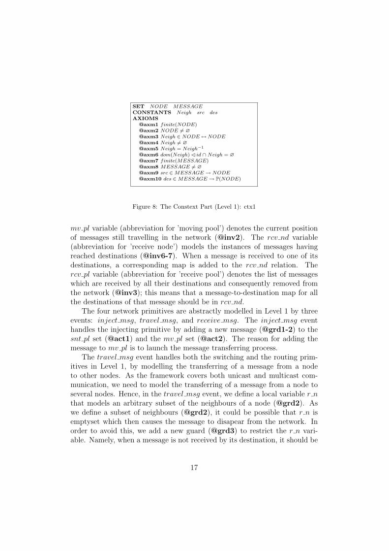
SET NODE MESSAGECONSTANTS Neigh src desAXIOMS
@axm1 finite(NODE)@axm2 NODE 6= ∅@axm3 Neigh ∈ NODE↔NODE@axm4 Neigh 6= ∅@axm5 Neigh = Neigh−1
@axm6 dom(Neigh)C id ∩ Neigh = ∅@axm7 finite(MESSAGE)@axm8 MESSAGE 6= ∅@axm9 src ∈MESSAGE → NODE@axm10 des ∈MESSAGE → P(NODE)
Figure 8: The Constext Part (Level 1): ctx1
mv pl variable (abbreviation for ’moving pool’) denotes the current positionof messages still travelling in the network (@inv2). The rcv nd variable(abbreviation for ’receive node’) models the instances of messages havingreached destinations (@inv6-7). When a message is received to one of itsdestinations, a corresponding map is added to the rcv nd relation. Thercv pl variable (abbreviation for ’receive pool’) denotes the list of messageswhich are received by all their destinations and consequently removed fromthe network (@inv3); this means that a message-to-destination map for allthe destinations of that message should be in rcv nd.
The four network primitives are abstractly modelled in Level 1 by threeevents: inject msg, travel msg, and receive msg. The inject msg eventhandles the injecting primitive by adding a new message (@grd1-2) to thesnt pl set (@act1) and the mv pl set (@act2). The reason for adding themessage to mv pl is to launch the message transferring process.
The travel msg event handles both the switching and the routing prim-itives in Level 1, by modelling the transferring of a message from a nodeto other nodes. As the framework covers both unicast and multicast com-munication, we need to model the transferring of a message from a node toseveral nodes. Hence, in the travel msg event, we define a local variable r nthat models an arbitrary subset of the neighbours of a node (@grd2). Aswe define a subset of neighbours (@grd2), it could be possible that r n isemptyset which then causes the message to disapear from the network. Inorder to avoid this, we add a new guard (@grd3) to restrict the r n vari-able. Namely, when a message is not received by its destination, it should be
17

invariants@inv1 snt pl ⊆MESSAGE@inv2 mv pl ∈ snt pl↔NODE@inv3 rcv pl ⊆MESSAGE@inv4 rcv pl ∩ dom(mv pl) = ∅@inv5 dom(mv pl) ∪ rcv pl = snt pl@inv6 rcv nd ∈ NODE↔MESSAGE@inv7 ∀msg, d·d 7→ msg ∈ rcv nd⇒ d ∈ des(msg)@inv8 ∀msg ·msg ∈ dom(mv pl)⇒ (∃d·d ∈ des(msg) ∧ d 7→ msg /∈ rcv nd)@inv9 ∀msg ·msg ∈ rcv pl⇔ (∀d·d ∈ des(msg)⇒ d 7→ msg ∈ rcv nd)@inv10 ran(rcv nd) ⊆ snt pl@inv11 ∀msg ·msg ∈ snt pl ∧ des(msg) \ rcv nd−1[{msg}] 6= ∅ ⇒ msg ∈
dom(mv pl)@inv12 mv pl = ∅⇒ ran(rcv nd) = snt pl
inject msgany msgwhere
@grd1 msg ∈MESSAGE@grd2 msg /∈ snt pl
then@act1 snt pl := snt pl ∪ {msg}@act2 mv pl := mv pl ∪ {msg 7→ src(msg)}
end
travel msgany msg n r nwhere
@grd1 msg 7→ n ∈ mv pl@grd2 r n ⊆ Neigh[{n}]@grd3 (n /∈ des(msg) ∧ r n 6= ∅) ∨ (n 7→ msg ∈ rcv nd ∧ (∃m·msg 7→ m ∈ mv pl∧n 6= m)) ∨ (n 7→ msg ∈ rcv nd ∧ (∀m·msg 7→ m ∈ mv pl⇒ n = m) ∧ r n 6= ∅)
then@act1 mv pl := (mv pl \ {msg 7→ n}) ∪ ({msg} × r n)
end
received msgany msg n rcvwhere
@grd1 msg 7→ n ∈ mv pl@grd2 n ∈ des(msg)@grd3 rcv ⊆MESSAGE@grd4 ((∃d·d ∈ des(msg) ∧ d 7→ msg /∈ rcv nd ∪ {n 7→ msg}) ∧ rcv = ∅)∨((∀d·d ∈ des(msg)⇒ d 7→ msg ∈ rcv nd ∪ {n 7→ msg}) ∧ rcv = {msg})
then@act1 rcv nd := rcv nd ∪ {n 7→ msg}@act2 rcv pl := rcv pl ∪ rcv@act3 mv pl := rcv C−mv pl
end
Figure 9: The Machine Part (Level 1): M1
18

routed next and should not be removed from the network. This condition ismodelled by the first or (∨) part of the @grd3. The second or part of the@grd3 models the state when the current position of the message is one ofits destinations and there are other instances of the message in the network.In this case r n can be either an emptyset or a subset of neighbours. Thelast or part of the @grd3 restricts the r n to a non-emptyset when the cur-rent position is one of its destinations and the last instance of the messageis in this position. Without the last condition of @grd3, we could removethe message from the network when the message is not yet received by allits destinations. We note that we postpone the modelling of specific routingand switching primitives for the subsequent refinement steps; however, weadd the necessary conditions so that any switching and routing primitivescan be derived out of the travel msg event.
The receive msg event handles the receiving primitive of the networkmodel in two different situations. Either the message is received by all itsdestinations or, there are still some destinations that did not receive themessage. To specify two different situations in one event, we define a localvariable rcv, which is a subset of messages (@grd3). When there are stillsome destinations that did not received the message, the rcv variable is setto empty, as shown by the first or part of @grd4. When the message isreceived by all its destinations, the rcv variable is set to the message, shownby the second or part of @grd4. When there are still some destinations thatdid not received the message, the corresponding message-to-destination mapis added to rcv nd (@act1) and the message is not added to rcv pl becausethere are still destinations waiting for it. When the message is received byall its destinations, the message is also added to the rcv pl (@act2) andremoved from the mv pl (@act2).
To guarantee the functional correctness of our modelling, we specify theproperties of the network as a list of invariants shown in Fig. 9. The first threeinvariants (@inv1-3) and @inv6 are for variable definitions and the remain-ing invariants illustrate the correctness properties of network that should bepreserved by all the events. While messages are travelling in the network,they are not received by all their destinations (@inv8, 11) and when a mes-sage is received at all its destinations, then there should not be any instanceof that message in the network, shown by @inv4; moreover, it should be inthe received state, shown by @inv9. As we model a network without messageloss, we should guarantee that an injected message is either in the travellingstate or received state and this property is shown by @inv5. The rcv nd
19

models messages which are received at destination: the rcv nd relation canonly consist of node−msg pairs where node is one of the destinations of msg(shown by @inv7). When no messages is in the travelling state it means thatall the injected messages are received by all their destinations, as formulatedby @inv12.
The correctness verification of the initial model in which only the Node
subcomponent of the Structural Elements is specified is performed byproving the satisfiability of invariants by events and the well-definednessof the events’ guards. The number of proof obligations that are generatedand the number of proof obligations that either automatically or manuallydischarged are shown in Table. 1.
Table 1: Proof Statistics Level 1Model Number of Proof Automatically Interactively
Obligations Discharged Discharged
Level1 Context 2 2(100%) 0(0%)
Level1 Machine 39 32(82%) 7(18%)
The initial model forms the first hierarchical level, Level 1, of our devel-opment. Level 1 is a foundation model for the subsequent refinement steps,where we refine the context part of the model to extend the network architec-ture and refine the machine part of the model to refine the network primitives.The relation between our refinement levels is illustrated in Fig. 10.
5.2. Specification of the NetCorre: Level 2
In Level 2, we extend the initial context to model the Channel struc-tural element. We specify the set CHANNEL that (physically) connectsneighbour nodes to each other. In other words, for any pair in the Neighrelation, we model a channel that connects the pair by modelling two func-tions: start ch nd (abbreviation for ’start channel from node’) (@axm11)and end ch nd (abbreviation for ’end channel to node’) (@axm12). In orderto show the new channel relations correspond to the neighbour relations, wespecify that the bidirectional links between two neighbours corresponded tothese new relations (@axm13). Moreover, we model that the composition ofthese two relations is equal to Neigh relation (@axm14) as shown in Fig. 11.
At this level we refine the network primitive component to specify thetransferring of messages through the channels. In this level of the hierarchy,we use the data refinement technique. In the initial model, the mv pl re-lation denotes the current position of messages in the network. In order to
20

Figure 10: Network Scheme in Event-B
SETS CHANNELCONSTANTS start ch nd end ch ndAXIOMS
@axm11 start ch nd ∈ CHANNEL→ NODE@axm12 end ch nd ∈ CHANNEL→ NODE@axm13 ∀n, ch·ch 7→ n ∈ start ch nd ⇒ (∃ch2·ch2 7→ end ch nd(ch) ∈
start ch nd∧ch2 7→ n ∈ end ch nd)
@axm14 Neigh ∪ (dom(Neigh)C id) = start ch nd−1; end ch nd
Figure 11: The Context Part (Level 2): ctx2
21

invariants@inv13 mv nd ∈ snt pl↔NODE@inv14 mv ch ∈ snt pl↔ CHANNEL@inv15 mv ch−1 ∈ CHANNEL 7→ snt pl@inv16 (mv ch; start ch nd) ∪ mv nd = mv pl@inv17 ∀ch,msg ·msg 7→ ch ∈ mv ch⇒ ((start ch nd(ch) /∈ des(msg))∨(start ch nd(ch) 7→ msg ∈ rcv nd ∧msg /∈ rcv pl))
Figure 12: The Machine Part (Level 2): Invariants
represent the existence of messages in both nodes and channels, in the secondmodel we replace the mv pl variable with two variables: mv nd (abbreviat-ing for ’moving node pool’) and mv ch (abbreviating for ’moving channelpool’), shown in Fig. 12. The mv nd variable denotes the current positionof those messages that are in nodes ( @inv13) and the mv ch variable de-notes the current position of those messages that are in channels (@inv14).At any moment, any channel can be either free or busy with only one mes-sage, described by invariant (@inv15). Moreover, the union of messages inthe (mv ch; start ch nd) and mv nd relations is equal to those messages inmv pl, described by the gluing invariant @inv16 in Fig. 12. A message istransferred from a node to a channel if the node is not one of the messagedestinations or the node is a message destination but the message is notreceived by all its destinations, formulated by @inv17.
As a consequence of this data refinement, the events that model thenetwork primitive component are updated, so that all the connections tomv pl are substituted either by mv nd or by mv ch. In addition, we re-fine the travel msg event by splitting it into two events: travel to ch andtravel to nd, shown in Fig. 13. The travel to ch event models the transfer-ring of a message from a node to a channel at the beginning of the channel.When there is a message at a node (travel to ch: @grd1), a subsets of out-put channels of the node (@grd2, correponding to @grd2 in travel msg inLevel 1) which are free (@grd4) are chosen for transferring. The channelselection is restricted by considering three different situations correspondingto @grd3 in travel msg in Level 1. First, when the current node is not adestination of the message the subset of channels cannot be empty becausethe message should travel through another node, as described by the firstor part of @grd3. Second, when the current node is one of the messagedestinations and another instance of a message in other nodes exists in the
22

network, then in this state, any arbitrary set of the output channels can beselected, as described by the second or part of @grd3. Last, when the cur-rent node is one of the message destinations and no instance of the messageexists in the network, then the subset of channels cannot be empty becausethe message might still have some destinations to reach. This is describedby the last or part of @grd3. As it is described, @grd3 of the travel to chevent is the refinement of the @grd3 of the travel msg event in Level 1.In the with part of the travel to ch event, the witness is specified for theabstract parameter r n of the abstract event travel msg and its feasibility isgiven by axiom @axm14. This axiom is ’gluing’ the constant Neigh fromLevel 1 to constants start ch nd and end ch nd from Level 2.
When the travel to ch event is executed the instance of the message in thecurrent node is either removed from the mv nd or remains in mv nd, depend-ing on whether the message is routed to all the selected channels according toa routing algorithm. In a state when all routes are not free the transferringthe message should wait in the current node until the desired channels be-come free. This assignment (shown by @act1) is non-deterministic so thatthe event covers all possible situations of data transferring in a node. Finally,the transferring of a message from a node to the selected subset of channelsis modelled by @act2.
The travel to nd event models the transferring of a message from a chan-nel to a node at the end of the channel. The travel to nd event is enabledwhen there is a message in a channel (@grd1). This event removes themessage from the channel (@act1) and adds it to the node at the end ofthe channel (@act2). As the abstract parameters n and r n are removedin this refined event, we define witnesses for them based on the new in-troduced parameter ch to be sure about the correctness of the refinement.The n parameter is equal to the node at the start point of the channel andr n, which models neighbours of node n, is equal to the node at the end ofthe channel, described in the with part of the travel to nd event. The useof witnesses adds clarity to a refined model and determining the requiredwitnesses is often straightforward. The witnesses are also used to generatesimpler invariant preservation proof obligations by decomposing proof obli-gations which, otherwise, would contain the existentailly quantified formulain their hypothesis.
This data refinement comes with a list of proof obligations that expressits correctness. These obligations guarantee that the second model preservesthe network properties component and its statistics are shown in Table 2.
23

travel to chrefines travelany msg n chwhere
@grd1 msg 7→ n ∈ mv nd@grd2 ch ⊆ start ch nd−1[{n}]@grd3 (n /∈ des(msg) ∧ ch 6= ∅) ∨ (n 7→ msg ∈ rcv nd∧(∃m·msg 7→ m ∈ (mv ch; start ch nd) ∪ mv nd ∧ n 6= m))∨(n 7→ msg ∈ rcv nd∧ (∀m·msg 7→ m ∈ (mv ch; start ch nd) ∪mv nd⇒ n = m)∧ ch 6= ∅)@grd4 ran(mv ch) ∩ ch = ∅
with r n : r n ⊆ (start ch nd−1; end ch nd)[{n}]then
@act1 mv nd : | mv nd′ = mv nd \ {msg 7→ n} ∨mv nd′ = mv nd@act2 mv ch := mv ch ∪ ({msg} × ch)
end
travel to ndrefines travelany msg chwhere
@grd1 msg 7→ ch ∈ mv chwithn : n = start ch nd(ch)r n : r n = end ch nd(ch)
then@act1 mv ch := mv ch \ {msg 7→ ch}@act2 mv nd := mv nd ∪ {msg 7→ end ch nd(ch)}
end
Figure 13: The Machine Part (Level 2): Events
An Extra Refinement Step.. To avoid adding too much complexity tothe specification, @act1 in travel to ch is modelled as a non-deterministicassignment in Level 2. A message in a node can be sent to a number of outputchannels depending on the routing decisions. If a message is transferred toall the selected channels, the message is removed from mv nd. Otherwise,the mv nd remains unchanged. Here we add a new variable waiting msgwhich models the list of output channels of any node that waits for messagesto be transferred, as shown by @inv18 in Fig. 14.
When a node makes a decision about routing a message to different outputchannels, the node sends the message to all the selected channels providedthat the selected channels are free; in this case the instance of the message isremoved from the node. Otherwise, the message is sent to the free selectedchannels and waits for the other selected channels to become free. Once themessage is sent to all the selected channels, the instance of the message is re-
24

Table 2: Proof Statistics Level 2Model Number of Proof Automatically Interactively
Obligations Discharged Discharged
Level2 Context 1 1(100%) 0(0%)
Level2 Machine 67 47(70%) 20(30%)
invariants@inv18 waiting msg ∈ mv nd↔ CHANNEL@inv19 ∀msg, ch ·msg 7→ ch ∈ mv ch ⇒ msg 7→ start ch nd(ch) 7→ ch /∈
waiting msg@inv20 ∀msg, n, ch ·msg 7→ n 7→ ch ∈ waiting msg⇒ start ch nd(ch) = n
Figure 14: The Extra Refinement Step Machine Part: Invariants
moved from the node. The waiting msg variable denotes the messages whichare not transferred to the selected channels. Once a message is transferredto a selected channel, the message, which was waiting for that channel, is re-moved from the waiting msg, illustrated by @inv19. In addition, we needto guarantee that when a message is about to be sent to output channelsof a node, this means that the node is at the start point of these selectedchannels, shown by @inv20.
At this level, we split (via refinement) the travel to ch event to threetravel to ch ncmpl, travel to ch cmp and waiting list events to remove thenon-deterministic assignment in the abstract event as shown in Fig. 15. Weuse the group refinement technique in this level to indicate the requiredevent ordering, as provided by the group refinement technique. In our grouprefinement, the waiting list event is the first event in the trace and thetravel to ch cmp is the last event in the trace.
In the waiting list event, when there is a message at a node (@grd1)and the routing decision has not been taken for the message in the node(@grd3), an arbitrary number of output channels of the node are selected(@grd2). The @grd4 in waiting list event expresses the same condition asthe @grd4 in the abstract travel to ch event. The waiting msg is updatedby adding the triple of message, node and the selected output channels, shownby @act1.
After the waiting list event, either travel to ch cmp or travel to ch ncmpare enabled depending on the availability of the selected output channels.As removing a pair of message and node from mv nd means transferring the
25
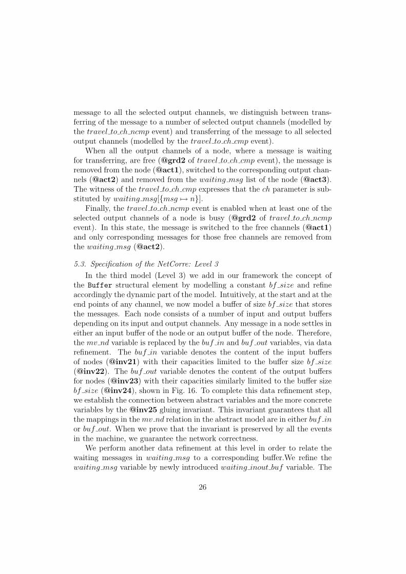
message to all the selected output channels, we distinguish between trans-ferring of the message to a number of selected output channels (modelled bythe travel to ch ncmp event) and transferring of the message to all selectedoutput channels (modelled by the travel to ch cmp event).
When all the output channels of a node, where a message is waitingfor transferring, are free (@grd2 of travel to ch cmp event), the message isremoved from the node (@act1), switched to the corresponding output chan-nels (@act2) and removed from the waiting msg list of the node (@act3).The witness of the travel to ch cmp expresses that the ch parameter is sub-stituted by waiting msg[{msg 7→ n}].
Finally, the travel to ch ncmp event is enabled when at least one of theselected output channels of a node is busy (@grd2 of travel to ch ncmpevent). In this state, the message is switched to the free channels (@act1)and only corresponding messages for those free channels are removed fromthe waiting msg (@act2).
5.3. Specification of the NetCorre: Level 3
In the third model (Level 3) we add in our framework the concept ofthe Buffer structural element by modelling a constant bf size and refineaccordingly the dynamic part of the model. Intuitively, at the start and at theend points of any channel, we now model a buffer of size bf size that storesthe messages. Each node consists of a number of input and output buffersdepending on its input and output channels. Any message in a node settles ineither an input buffer of the node or an output buffer of the node. Therefore,the mv nd variable is replaced by the buf in and buf out variables, via datarefinement. The buf in variable denotes the content of the input buffersof nodes (@inv21) with their capacities limited to the buffer size bf size(@inv22). The buf out variable denotes the content of the output buffersfor nodes (@inv23) with their capacities similarly limited to the buffer sizebf size (@inv24), shown in Fig. 16. To complete this data refinement step,we establish the connection between abstract variables and the more concretevariables by the @inv25 gluing invariant. This invariant guarantees that allthe mappings in the mv nd relation in the abstract model are in either buf inor buf out. When we prove that the invariant is preserved by all the eventsin the machine, we guarantee the network correctness.
We perform another data refinement at this level in order to relate thewaiting messages in waiting msg to a corresponding buffer.We refine thewaiting msg variable by newly introduced waiting inout buf variable. The
26
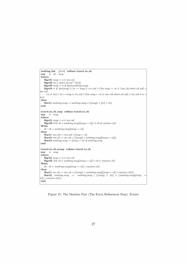
waiting list [first] refines travel to chany n ch msgwhere
@grd1 msg 7→ n ∈ mv nd@grd2 ch ⊆ start ch nd−1[{n}]@grd3 msg 7→ n /∈ dom(waiting msg)@grd4 n /∈ des(msg) ∨ (n 7→ msg ∈ rcv nd ∧ (∃m·msg 7→ m ∈ (mv ch; start ch nd) ∪
mv nd∧n 6= m))∨ (n 7→ msg ∈ rcv nd∧ (∀m·msg 7→ m ∈ (mv ch; start ch nd) ∪mv nd⇒ n =
m))then
@act1 waiting msg := waiting msg ∪ ({msg} × {n} × ch)end
travel to ch cmp refines travel to chany n msgwhere
@grd1 msg 7→ n ∈ mv nd@grd2 ∀ch·ch ∈ waiting msg[{msg 7→ n}]⇒ ch /∈ ran(mv ch)
Withch : ch = waiting msg[{msg 7→ n}]
then@act1 mv nd := mv nd \ {msg 7→ n}@act2 mv ch := mv ch ∪ ({msg} × waiting msg[{msg 7→ n}])@act3 waiting msg := {msg 7→ n}C− waiting msg
end
travel to ch ncmp refines travel to chany n msgwhere
@grd1 msg 7→ n ∈ mv nd@grd2 ∃ch·ch ∈ waiting msg[{msg 7→ n}] ∧ ch ∈ ran(mv ch)
Withch : ch = waiting msg[{msg 7→ n}] \ ran(mv ch)
then@act1 mv ch := mv ch ∪ ({msg} × (waiting msg[{msg 7→ n}] \ ran(mv ch)))@act2 waiting msg := waiting msg \ ({msg} × {n} × (waiting msg[{msg 7→
n}] \ ran(mv ch)))end
Figure 15: The Machine Part (The Extra Refinement Step): Events
27
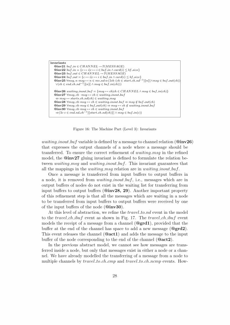
invariants@inv21 buf in ∈ CHANNEL→ P(MESSAGE)@inv22 buf in = {c 7→ i|c 7→ i ∈ buf in ∧ card(i) ≤ bf size}@inv23 buf out ∈ CHANNEL→ P(MESSAGE)@inv24 buf out = {c 7→ i|c 7→ i ∈ buf in ∧ card(i) ≤ bf size}@inv25 ∀msg, n·msg 7→ n ∈ mv nd⇒(∃ch·(ch ∈ start ch nd−1[{n}]∧msg ∈ buf out(ch))∨(ch ∈ end ch nd−1[{n}] ∧msg ∈ buf in(ch)))
@inv26 waiting inout buf = {msg 7→ ch|ch ∈ CHANNEL ∧msg ∈ buf in(ch)}@inv27 ∀msg, ch ·msg 7→ ch ∈ waiting inout buf⇔ msg 7→ starts ch nd(ch) ∈ waiting msg
@inv28 ∀msg, ch·msg 7→ ch ∈ waiting inout buf ⇒msg /∈ buf out(ch)@inv29 ∀msg, ch·msg ∈ buf out(ch)⇒msg 7→ ch /∈ waiting inout buf@inv30 ∀msg, ch·msg 7→ ch ∈ waiting inout buf⇒(∃c·c ∈ end nd ch−1[{start ch nd(ch)}] ∧msg ∈ buf in(c))
Figure 16: The Machine Part (Level 3): Invariants
waiting inout buf variable is defined by a message to channel relation (@inv26)that expresses the output channels of a node where a message should betransferred. To ensure the correct refinement of waiting msg in the refinedmodel, the @inv27 gluing invariant is defined to formulate the relation be-tween waiting msg and waiting inout buf . This invariant guarantees thatall the mappings in the waiting msg relation are in waiting inout buf .
Once a message is transferred from input buffers to output buffers ina node, it is removed from waiting inout buf , i.e., messages which are inoutput buffers of nodes do not exist in the waiting list for transferring frominput buffers to output buffers (@inv28, 29). Another important propertyof this refinement step is that all the messages which are waiting in a nodeto be transferred from input buffers to output buffers were received by oneof the input buffers of the node (@inv30).
At this level of abstraction, we refine the travel to nd event in the modelto the travel ch ibuf event as shown in Fig. 17. The travel ch ibuf eventmodels the receipt of a message from a channel (@grd1), provided that thebuffer at the end of the channel has space to add a new message (@grd2).This event releases the channel (@act1) and adds the message to the inputbuffer of the node corresponding to the end of the channel (@act2).
In the previous abstract model, we cannot see how messages are trans-ferred inside a node, but only that messages exist in either a node or a chan-nel. We have already modelled the transferring of a message from a node tomultiple channels by travel to ch cmp and travel to ch ncmp events. How-
28

travel ch ibufrefines travel to ndany ch msgwhere
@grd1 msg 7→ ch ∈ mv ch@grd2 card(buf in(ch)) < bf size
then@act1 mv ch := mv ch \ {msg 7→ ch}@act2 buf in(ch) := buf in(ch) ∪ {msg}
end
Figure 17: The Machine Part 1 (Level 3): Events
ever, in this refinement level, we detail on transferring messages inside thenodes. We consider moving messages from input buffers to output buffersand then from output buffers to channels. This view of the system givesthe idea of splitting each of the travel to ch cmp and travel to ch ncmpevents to two events. Therefore, we refine the travel to ch ncmp abstractevent to the travel to out buf ncmp and travel from buf to ch ncmp con-crete events as shown in Fig. 18. The travel to out buf ncmp event handlestransferring of a waiting message from an input buffer to output buffer andthe travel from buf to ch ncmp event deals with transferring of a waitingmessage from an output buffer to a channel. The same split is performed fortravel to ch cmp.
To transfer a message from an input buffer of a node to the selectedoutput buffers, we define a local variable avb buf in travel to out buf ncmpevent. The avb buf variable contains the list of output buffers selected fortransferring and with enough space to accept new messages (@grd2). Wedefine the avb buf local variable in the travel to out buf ncmp event becausewe need to exclude the selected output channels which are full and cannotreceive any messages (@grd1) from all the selected output channels.
In @act1 of travel to out buf ncmp, the message is added to the bufferslisted in avb buf . Moreover, the message waiting to be transferred to theoutput buffers, in avb buf , is removed from the waiting list (@act2). Wenote that the message is not removed from the input buffer because thereare instances of the message in the waiting list which are not transferredto output buffers. Removing the message from an input buffer of a node isdone when the message is transferred to all the selected output buffers, inwaiting inout buf and is modelled by the travel to out buf cmp event.
29
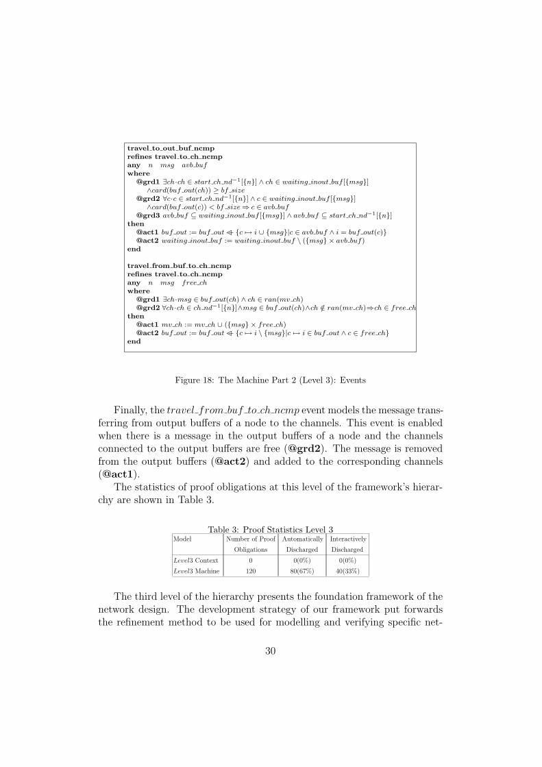
travel to out buf ncmprefines travel to ch ncmpany n msg avb bufwhere
@grd1 ∃ch·ch ∈ start ch nd−1[{n}] ∧ ch ∈ waiting inout buf [{msg}]∧card(buf out(ch)) ≥ bf size
@grd2 ∀c·c ∈ start ch nd−1[{n}] ∧ c ∈ waiting inout buf [{msg}]∧card(buf out(c)) < bf size⇒ c ∈ avb buf
@grd3 avb buf ⊆ waiting inout buf [{msg}] ∧ avb buf ⊆ start ch nd−1[{n}]then
@act1 buf out := buf outC− {c 7→ i ∪ {msg}|c ∈ avb buf ∧ i = buf out(c)}@act2 waiting inout buf := waiting inout buf \ ({msg} × avb buf)
end
travel from buf to ch ncmprefines travel to ch ncmpany n msg free chwhere
@grd1 ∃ch·msg ∈ buf out(ch) ∧ ch ∈ ran(mv ch)@grd2 ∀ch·ch ∈ ch nd−1[{n}]∧msg ∈ buf out(ch)∧ch /∈ ran(mv ch)⇒ch ∈ free ch
then@act1 mv ch := mv ch ∪ ({msg} × free ch)@act2 buf out := buf outC− {c 7→ i \ {msg}|c 7→ i ∈ buf out ∧ c ∈ free ch}
end
Figure 18: The Machine Part 2 (Level 3): Events
Finally, the travel from buf to ch ncmp event models the message trans-ferring from output buffers of a node to the channels. This event is enabledwhen there is a message in the output buffers of a node and the channelsconnected to the output buffers are free (@grd2). The message is removedfrom the output buffers (@act2) and added to the corresponding channels(@act1).
The statistics of proof obligations at this level of the framework’s hierar-chy are shown in Table 3.
Table 3: Proof Statistics Level 3Model Number of Proof Automatically Interactively
Obligations Discharged Discharged
Level3 Context 0 0(0%) 0(0%)
Level3 Machine 120 80(67%) 40(33%)
The third level of the hierarchy presents the foundation framework of thenetwork design. The development strategy of our framework put forwardsthe refinement method to be used for modelling and verifying specific net-
30

work designs. As demonstrated, in each hierarchical level we gradually addmore elements and primitives together their corresponding properties to theabstract level until we achieve a more detailed model of the system. Thismethod allows us to understand the problem from various facets, while wefocus on the various parts of the system at each level.
We also note the integration aspect of our framwork. For instance, inLevel 2 we add the Channel structural element to the network architecturemodel and at the same time, we need to develop the network primitives interms of this element. The correctness of the algorithm-architecture integra-tion is expressed by the model invariants that are proved correct for all thenetwork primitives (i.e., algorithm) and elements (i.e., architecture).
6. A Theory Basis for the NetCorre framework
Based on the developed NetCorre framework put forward in the previoussection, we now extract a network theory to be reused in concrete networkmodelling. NetCorre is independent of any design details and its componentscan be easily refined to concrete models until, e.g. a concrete routing algo-rithm is derived [13]. Each component (architectural or primitives) can berefined to different instances and the same instance of a component can beused in different network developments, e.g. to develop a FIFO-buffer [13].Hence, it is imperative to raise the reusability of our framework to a moreprominent level. For this, we build a library of pre-defined and pre-provedreusable units of the framework to be employed in various network design.This approach dramatically improves the lifecycle modelling and proving net-work designs. To produce a library of reusable units, we adapt the idea ofobject-oriented inheritance in which a root class is defined and then extendedto other classes. Therefore, in this section the fundamental components ofnetwork design are defined as root classes by defining and proving theoremsfor these components. The introduced theorems are the design rules of ourmethodology; they can be extended to particular component developmentsand then used in refined models of the network.
In the rest of this section, we extend the mathematical language andtheory of Event-B to specify the most relevant characteristics of networkdesign in a network extension. This network extension encompasses def-initions and properties from NetCorre that we deem fundamental for anynetwork design. In other words, the proposed network extension consists ofthe NetCorre components that can be reused to specify and verify different
31

network designs. We introduce new predicate definitions, new operator defi-nitions and theorems dedicated to network designs. The purpose of the newnetwork extension is to avoid remodelling and especially reproving modelproperties every time we need a formal network design. Instead, we providea pre-defined and pre-proved library containing fundamental characteristicsof networked systems. We develop the network extension by using the theoryplug-in. The proposed network extension provides a means for designers todevelop various network models when the developments do not contradictthe network theory.
We develop three theory levels, N1-N3, following the development orderof NetCorre. Hence, the Event-B theory corresponding to the hierarchicalframework is developed in a hierarchical manner as well. The overview ofhierarchical development is shown in Fig. 19.
Figure 19: Network Theory of the Framework
32
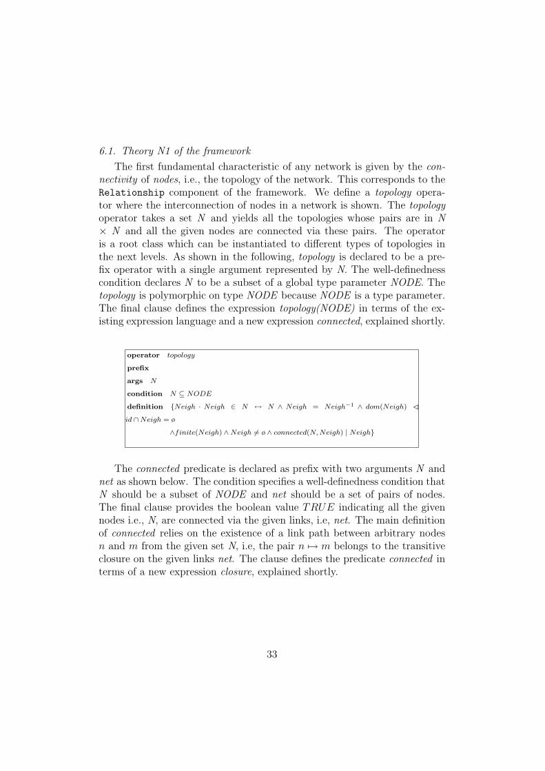
6.1. Theory N1 of the framework
The first fundamental characteristic of any network is given by the con-nectivity of nodes, i.e., the topology of the network. This corresponds to theRelationship component of the framework. We define a topology opera-tor where the interconnection of nodes in a network is shown. The topologyoperator takes a set N and yields all the topologies whose pairs are in N× N and all the given nodes are connected via these pairs. The operatoris a root class which can be instantiated to different types of topologies inthe next levels. As shown in the following, topology is declared to be a pre-fix operator with a single argument represented by N. The well-definednesscondition declares N to be a subset of a global type parameter NODE. Thetopology is polymorphic on type NODE because NODE is a type parameter.The final clause defines the expression topology(NODE) in terms of the ex-isting expression language and a new expression connected, explained shortly.
operator topology
prefix
args N
condition N ⊆ NODEdefinition {Neigh · Neigh ∈ N ↔ N ∧ Neigh = Neigh−1 ∧ dom(Neigh) Cid ∩Neigh = ø
∧finite(Neigh) ∧Neigh 6= ø ∧ connected(N,Neigh) | Neigh}
The connected predicate is declared as prefix with two arguments N andnet as shown below. The condition specifies a well-definedness condition thatN should be a subset of NODE and net should be a set of pairs of nodes.The final clause provides the boolean value TRUE indicating all the givennodes i.e., N, are connected via the given links, i.e, net. The main definitionof connected relies on the existence of a link path between arbitrary nodesn and m from the given set N, i.e, the pair n 7→ m belongs to the transitiveclosure on the given links net. The clause defines the predicate connected interms of a new expression closure, explained shortly.
33

predicate connected
prefix
args N net
condition N ⊆ NODE ∧ net ⊆ NODE ↔ NODE
definition ∃c·c ∈ closure(net)∧(∀n,m·n ∈ N∧m ∈ N ⇒ n 7→ m ∈ c)
The closure operator is declared as prefix with an argument net. Thecondition specifies a well-definedness condition that net should be a set ofpairs of nodes. The final clause provides the transitive closure of a binaryrelation on the set of pairs.
operator closure
prefix
args net
condition net ⊆ NODE ↔ NODE
definition {cl · cl ∈ NODE ↔ NODE ∧ net ⊆ cl ∧ cl;net ⊆ cl∧(∀s · net ⊆ s ∧ s;net ⊆ s⇒ cl ⊆ s) | cl}
Having introduced those new predicates and operators, we specify andprove theorems about them. The aim is to develop a library of rules derivedfrom the introduced operators and to provide the possibility to prove anynewly introduced theorem. The introduced theorems can then be used inthe rule form in proofs.
The following theorems show the properties which should be preservedregarding the connected operator. The first theorem shows that an emptyset of nodes is connected in any networks and the second one denotes thatany subset of nodes connected in a sub-network are also connected on largernetworks that include the sub-network. The last theorem denotes that whena set of nodes is connected in a network, any subsets of the set is also con-nected in the network. We note that any instances of the topology operatorinherits all its proved theorems regarding connectivity.
34

thm emptyset ∀L · L ∈ NODE ↔ NODE ⇒ connected(∅, L)
thm subnetCon ∀S,L, L2 · L ∈ NODE ↔ NODE ∧ L2 ∈ NODE ↔ NODE
∧L ⊆ L2 ∧ connected(S,L)⇒ connected(S,L2)
thm subnodeCon ∀S1, S2, L · L ∈ NODE ↔ NODE ∧ S1 ∈ P (NODE)
∧S2 ∈ P (NODE) ∧ S1 ⊆ S2 ∧ connected(S2, L)⇒ connected(S1, L)
The abstract architecture component of the framework can be developedby applying these operators in the system development phase. The abstractNetwork primitives component of the framework consists of Injecting,Routing and Receiving; abstract operator for each of them is put forwardin this section. The injection operator models the abstract behaviour ofinjecting sub-component of NetCorre by getting a list of messages and anetwork topology. The operator maps the list of messages to a number ofnodes of a network. We note that we do not model details of messages suchas source and destinations and these details can be defined later in a networkmodel.
operator injection
prefix
args msg net
condition net ∈ topology(NODE) ∧msg ⊆MSG
definition {in · in ∈ msg → dom(net) | in}
The routing operator models the behaviour of the routing componentin the framework by getting a list of messages with their location in thenetwork and a network topology. For each message in the list, the operatoreither keeps the message to its current position or transmits it to neighbournodes according to the topology given as an argument to the operator.
operator routing
prefix
args cur msg net
condition net ∈ topology(NODE) ∧ cur msg ∈MSG↔ dom(net)
definition {next ·next ∈ dom(cur msg)↔ dom(net)∧ dom(next) = dom(cur msg)
∧ next ⊆ cur msg;net ∧ next 6= cur msg | next}
35

The routing operator is a reusable unit which acts as a root class in ourdevelopment to instantiate different routing algorithms. The instantiatedrouting algorithms inherit all the proved properties of the routing operatorand then they can be used in the development of particular networks.
The received operator is declared to be a prefix operator with two argu-ments: msg and net. The well-definedness conditions declare msg to be asubset of a global type parameter MSG and net to be a relation, containingNODE ↔ NODE pairs. The final clause defines the expression received interms of the newly introduced network expression language.
operator received
prefix
args msg net
condition net ∈ topology(NODE) ∧msg ⊆MSG
definition {out · out ∈ msg ↔ dom(net) ∧ dom(out) = msg
∧ (∃in.in ∈ injection(msg, net)) | out}
Having introduced the operators for the network primitives, we spec-ify and prove theorems about their inter-relations. We develop a library ofrules derived from the introduced operators to provide a means for users toverify the correctness of a network design by using these theorems in proofs.The first theorem denotes that no messages are lost during routing and thesecond one shows that for any set of messages injected to the network, thereis the set of messages which are received by the nodes of the network.
thm NoMsgLoss in Routing ∀net, next,m, in m · net ∈ topology(NODE)
∧ in m ∈ injection(MSG,net) ∧m ∈ dom(in m) 7→ dom(net)
∧ next ∈ routing(net,m)⇒ dom(next) = dom(m)
thm InjectionReceivedEquality ∀net, rcv, in m · net ∈ topology(NODE)
∧ in m ∈ injection(MSG,net) ∧ rcv ∈ received(dom(in m), net)
⇒ dom(rcv) = dom(in m)
6.2. Theory N2 of the framework
The development of the theory follows the hierarchical development ofthe framework because the proposed hierarchy suits the construction of a
36

well-structured theory of the network. Therefore, to extend Level 1 of thehierarchical framework and model the Channel structural element, we createa new theory component N2 where N1 theory component is imported. TheN2 theory component has a CH global type parameter used in operator def-initions. To express channels as a data transferring media, the global typeparameter CHANNEL should be connected to the topology concept definedby the topology operator. Channels connect neighbour nodes to each other,i.e., all pairs of nodes in any topology should be represented via channels.Therefore, two new operators input ch and output ch are introduced in N2.The input ch operator is defined in the following way:
operator input ch
prefix
args c net
condition c ⊆ CHANNEL ∧ net ∈ topology(NODE)
definition{sc · sc ∈ c� net | (sc; (net C prj1))−1}
The input ch operator is declared as prefix with two arguments c and net.The condition specifies a well-definedness condition that c must be a subsetof CHANNEL and net must be of type topology(NODE). The final clauseprovides the definition of the expression input ch(CH, NODE ↔ NODE) interms of the N1 expression language. The definition declares mapping ofchannels to nodes that are connected to other nodes as shown in the topologydefinition.
For defining the output ch operator we have three arguments c, net andsc. The condition specifies that c must be a subset of CHANNEL, net mustbe of type topology(NODE) and sc must be of type input ch(c, net). Theoperator definition means that for any set of channels mapped to nodes byinput ch operator, a corresponding node to channel mapping is constructedin such a way that the composition of these two mapping is equal to thegiven topology.
37

operator output ch
prefix
args c net sc
condition c ⊆ CHANNEL ∧ net ∈ topology(NODE) ∧ sc ∈ input ch(c, net)
definition{ch nd, ec ·ch nd ∈ c� net∧ec = ch nd; (net C prj1)∧sc; ec = net | ec−1}
Besides, we specify theorems about channel structural elements and ex-tend the proposed library of rules for network modelling. The first theoremshows that any channel is mapped to only one pair of nodes. In other words,the reverse of a derived relation from output ch operator is a function. Thesecond theorem denotes that given a network topology and a set of channels,the input ch and output ch operators can construct exactly the same topol-ogy plus more information about channels. This means that without consid-ering channels in derived relations from input ch and output ch, we achievethe given topology. We note that both input ch and output ch are extensionsof the topology operator in the N1 theory of the hierarchical framework. Inother words, these two newly introduced operators are an implementation ofthe topology operator in the N1 theory.
thm Rev ch fun ∀n, c, net, sc, ec ·n ⊆ NODE ∧ c ⊆ CHANNEL∧net ∈ topology(n)
∧ sc ∈ input ch(c, net) ∧ ec ∈ output ch(c, net, sc)⇒ ec ∈ n↔ c ∧ ec−1 ∈ c→ n
thm chNet eq to ch ∀n, c, net, sc, ec · n ⊆ NODE ∧ c ⊆ CHANNEL ∧ net ∈topology(n)
∧ sc ∈ input ch(c, net) ∧ ec ∈ output ch(c, net, sc)⇒ sc; ec−1 = net
6.3. Theory N3 of the framework
The third level of the hierarchical framework NetCorre introduces thebuffer structural element; correspondingly, we create a new theory com-ponent to define rules about buffers where the N2 theory component is im-ported. We define a new inductive datatype to represent buffers; this canthen be used to define the enqueue and dequeue operators for specific typesof buffers. The buffer constructors consist nil and cons that seperate formsthat an element might take. The cons constructor composed of two destruc-tors of head and tail that provide a means of accessing the feild of an element.
38

datatypes buffer
type arguments MESSAGE
constructors
nil
cons
destructors
head type MESSAGE
tail type buffer(MESSAGE)
6.4. Using the Theory of the framework
These three network theory levels form the basis of design rules in ourmethodology and any extension of these rules adds an instance of the networkcomponents to the library of design rules. As an example of extending thetheory Level N3, the enqueue and dequeue operators of a FIFO-buffer areillustrated in the following.
The enqueue operator is declared to be a prefix operator with two ar-guments, buf and msg; it models the adding of the new message msg tothe top of the queue buf . The dequeue operator is defined to be a prefixoperator with the argument buf and models the removal of the message atthe bottom of the queue buf . The functioning of the operators is ensuredwith the theorems thm1, thm2, and thm3.
operator FIFO enqueue
prefix
args buf msg
condition buf ∈ buffer(msg)∧ msg ∈MESSAGE
definition cons(m, b)
operator FIFO dequeue
prefix
args buf
condition buf ∈ buffer(msg)∧ buf 6= nil
recursive definition match buf
nil : b
cons(x, a) : if a = nil then nil
else cons(x, FIFO dequeue (a,msg))
39

operator FIFO delete
prefix
args buf msg
condition buf ∈ buffer(msg) ∧msg ∈MESSAGE
recursive definition match buf
(nil,msg) : nil
(cons(x, a),msg) : if x = m then
FIFO delete(a) else
cons(x, FIFO delete(a,msg))
operator FIFO size
prefix
args buf
condition buf ∈ buffer(msg)recursive definition match buf
nil : 0
cons(x, a) : 1 +FIFO size(a)
thm1 ∀a, x.a ∈ buffer(MESSAGE)⇒ size(cons(x, a)) = size(a) + 1thm2 ∀b,m.m ∈MESSAGE ∧ b ∈ buffer(MESSAGE)
⇒ size(FIFO enqueue(b,m)) = size(b) + 1thm3 ∀b.b ∈ buffer(MASSAGE) ⇒ size(FIFO dequeue(b)) =size(b)− 1
In Fig. 20 we point out the ‘position’ in the hierarchical development thatthe enqueue and dequeue operators for the FIFO buffer have. Other exten-sions can take place - we have depicted for the sake of example a ‘MinimalRouting’ theory in Fig. 20. In fact, any of the N1-N3 theory levels can beextended, as well as the newly developed ones such as the FIFO-buffer.
7. Conclusion
In this paper, we have introduced the hierarchical framework NetCorrefor correct network design, we have modeled it formally, and we have provenvarious properties about it. The instrumental formalism and tool supportin our modelling and proving endeavors is provided by the Event-B formalmethod and its associated Rodin platform. The formal design techniqueof refinement is at the centre of all our developments in this paper. It isthrough refinement that we are able to model a hierarchical framework andalso through refinement that the intended reuse of NetCorre is put forward.A network specification based on NetCorre can be refined until a network im-plementation is derived; some examples of derivations appear in [13]. Basedon NetCorre, we have defined and proved some fundamental ‘design rules’ fora network theory developed within the theory plugin of the Rodin toolset.These design rules can then be used to develop even more concrete design
40

Figure 20: Instantiation of Network Theory
41

rules, where precise definitions are proposed for the functional algorithms orarchitecture components.
We thus demonstrate that a systematic and effective specification andverification of various network designs is possible, based upon a small setof proved structural and functional network primitives, that are added ordetailed gradually. The framework allows to make a variety of design choicesin the early stages of the design with various degrees of modelling details,relying on the formal refinement technique. Our framework integrates boththe models for the algorithm and the architecture network design so that theoverall correctness is guaranteed.
We observe that our proposed NetCorre is very general, so that it canbe reused to model a wide variety of network designs. Remarkably, bothnetworks ‘in the large’ as well as networks-on-chip are approachable via ourframework, because defining NetCorre is based on previously engineeringnumerous networking models in Event-B [12, 14]. With NetCorre, we extractthe most general reusable network characteristics and put them up for furtherreuse.
References
[1] Abrial, J.: A System Development Process with Event-B and the RodinPlatform. chap. 1, pp. 1–3. Springer Berlin / Heidelberg, Berlin, Heidel-berg (2007). DOI http://dx.doi.org/10.1007/978-3-540-76650-6 1. URLhttp://dx.doi.org/10.1007/978-3-540-76650-6 1
[2] Abrial, J.: A system development process with event-b and the rodinplatform. Formal Methods and Software Engineering pp. 1–3 (2007)
[3] Abrial, J.R.: Modeling in Event-B: System and Software Engineering.Cambridge University Press (2010)
[4] Abrial, J.R., Butler, M., Hallerstede, S., Hoang, T.S., Mehta, F.,Voisin, L.: Rodin: an open toolset for modelling and reason-ing in event-b. Int. J. Softw. Tools Technol. Transf. 12, 447–466 (2010). DOI http://dx.doi.org/10.1007/s10009-010-0145-y. URLhttp://dx.doi.org/10.1007/s10009-010-0145-y
[5] Abrial, J.R., Butler, M., Hallerstede, S., Leuschel, M., Schmalz, M.,Voisin, L.: Proposals for mathematical extensions for event-b. TechnicalReport
42

[6] Attiogbe, C.: Event-based approach to modelling dynamic architecture:Application to mobile ad-hoc network. In: ISoLA, pp. 769–781 (2008)
[7] Attiogbe, C.: Modelling and analysing dynamic decentralised systems.CoRR abs/0909.4896 (2009)
[8] Back, R.J.R., Kurki-Suonio, R.: Decentralization of process nets withcentralized control. In: Proceedings of the second annual ACM sympo-sium on Principles of distributed computing, PODC ’83, pp. 131–142.ACM, New York, NY, USA (1983). DOI 10.1145/800221.806716. URLhttp://doi.acm.org/10.1145/800221.806716
[9] Butler, M., Maamria, I.: Mathematical extension in event-b through therodin theory component. Technical Report
[10] Cansell, D., Mery, D., Proch, C.: System-on-chip design byproof-based refinement. Int. J. Softw. Tools Technol. Transf.11(3), 217–238 (2009). DOI 10.1007/s10009-009-0104-7. URLhttp://dx.doi.org/10.1007/s10009-009-0104-7
[11] Hoang, T.S., Kuruma, H., Basin, D.A., Abrial, J.R.: Developing topol-ogy discovery in event-b. In: IFM, pp. 1–19 (2009)
[12] Kamali, M., Laibinis, L., Petre, L., Sere, K.: Formal develop-ment of wireless sensoractor networks. Science of ComputerProgramming (0) (2012). DOI 10.1016/j.scico.2012.03.002. URLhttp://www.sciencedirect.com/science/article/pii/S0167642312000470?v=s5
[13] Kamali, M., Petre, L., Sere, K., Daneshtalab, M.: Correcomm: A formalhierarchical framework for communication designs. In: the 2nd IEEEInternational Conference on Embedded Systems for Enterprise Applica-tions. IEEE (2011)
[14] Kamali, M., Petre, L., Sere, K., Daneshtalab, M.: Formal modelingof multicast communication in 3d nocs. In: Digital System Design(DSD), 2011 14th Euromicro Conference on, pp. 634 –642 (2011). DOI10.1109/DSD.2011.86
[15] Kamali, M., Petre, L., Sere, K., Daneshtalab, M.: Refinement-basedmodeling of 3d nocs. In: Fundamental of Software Engineering (FSEN),
43

2011 4th IPM International Conference on, vol. 7141, pp. 236 –252.Springer-Verlag (2012)
[16] Lucarz, C., Mattavelli, M., Dubois, J.: A co-design platform for al-gorithm/architecture design exploration. In: Multimedia and Expo,2008 IEEE International Conference on, pp. 1069 –1072 (2008). DOI10.1109/ICME.2008.4607623
[17] Meng, Y.: Algorithm/architecture design space co-exploration for en-ergy efficient wireless communications systems. Ph.D. thesis, Santa Bar-bara, CA, USA (2006). AAI3233117
[18] Metayer, C., Voisin, L.: The Event-B Mathemati-cal Language (Version 2) (2009). URL http://deploy-eprints.ecs.soton.ac.uk/11/4/kernel lang.pdf
[19] Plosila, J., Sere, K.: Action systems in pipelined processor design. In:In Proc. of the 3rd Int. Symp. on Advanced Research in AsynchronousCircuits and Systems, pp. 156–166. IEEE Computer Society Press (1997)
[20] Rigorous Open Development Environment for Complex Systems(RODIN), IST FP6 STREP project [online]: Documentation athttp://rodin.cs.ncl.ac.uk/ (accessed 26 october 2011)
[21] RODIN tool platform [online]: Available at http://www.event-b.org/platform.html/ (Accessed 26 October 2011)
[22] Zhu, X., Malik, S.: A hierarchical modeling frameworkfor on-chip communication architectures of multiprocess-ing socs. ACM Trans. Des. Autom. Electron. Syst. 12(1),6:1–6:24 (2007). DOI 10.1145/1188275.1188281. URLhttp://doi.acm.org/10.1145/1188275.1188281
44

Turku Centre for Computer Science
TUCS Dissertations 1. Marjo Lipponen, On Primitive Solutions of the Post Correspondence Problem 2. Timo Käkölä, Dual Information Systems in Hyperknowledge Organizations 3. Ville Leppänen, Studies on the Realization of PRAM 4. Cunsheng Ding, Cryptographic Counter Generators 5. Sami Viitanen, Some New Global Optimization Algorithms 6. Tapio Salakoski, Representative Classification of Protein Structures 7. Thomas Långbacka, An Interactive Environment Supporting the Development of
Formally Correct Programs 8. Thomas Finne, A Decision Support System for Improving Information Security 9. Valeria Mihalache, Cooperation, Communication, Control. Investigations on
Grammar Systems. 10. Marina Waldén, Formal Reasoning About Distributed Algorithms 11. Tero Laihonen, Estimates on the Covering Radius When the Dual Distance is
Known 12. Lucian Ilie, Decision Problems on Orders of Words 13. Jukkapekka Hekanaho, An Evolutionary Approach to Concept Learning 14. Jouni Järvinen, Knowledge Representation and Rough Sets 15. Tomi Pasanen, In-Place Algorithms for Sorting Problems 16. Mika Johnsson, Operational and Tactical Level Optimization in Printed Circuit
Board Assembly 17. Mats Aspnäs, Multiprocessor Architecture and Programming: The Hathi-2 System 18. Anna Mikhajlova, Ensuring Correctness of Object and Component Systems 19. Vesa Torvinen, Construction and Evaluation of the Labour Game Method 20. Jorma Boberg, Cluster Analysis. A Mathematical Approach with Applications to
Protein Structures 21. Leonid Mikhajlov, Software Reuse Mechanisms and Techniques: Safety Versus
Flexibility 22. Timo Kaukoranta, Iterative and Hierarchical Methods for Codebook Generation in
Vector Quantization 23. Gábor Magyar, On Solution Approaches for Some Industrially Motivated
Combinatorial Optimization Problems 24. Linas Laibinis, Mechanised Formal Reasoning About Modular Programs 25. Shuhua Liu, Improving Executive Support in Strategic Scanning with Software
Agent Systems 26. Jaakko Järvi, New Techniques in Generic Programming – C++ is more Intentional
than Intended 27. Jan-Christian Lehtinen, Reproducing Kernel Splines in the Analysis of Medical
Data 28. Martin Büchi, Safe Language Mechanisms for Modularization and Concurrency 29. Elena Troubitsyna, Stepwise Development of Dependable Systems 30. Janne Näppi, Computer-Assisted Diagnosis of Breast Calcifications 31. Jianming Liang, Dynamic Chest Images Analysis 32. Tiberiu Seceleanu, Systematic Design of Synchronous Digital Circuits 33. Tero Aittokallio, Characterization and Modelling of the Cardiorespiratory System
in Sleep-Disordered Breathing 34. Ivan Porres, Modeling and Analyzing Software Behavior in UML 35. Mauno Rönkkö, Stepwise Development of Hybrid Systems 36. Jouni Smed, Production Planning in Printed Circuit Board Assembly 37. Vesa Halava, The Post Correspondence Problem for Market Morphisms 38. Ion Petre, Commutation Problems on Sets of Words and Formal Power Series 39. Vladimir Kvassov, Information Technology and the Productivity of Managerial
Work 40. Frank Tétard, Managers, Fragmentation of Working Time, and Information
Systems

41. Jan Manuch, Defect Theorems and Infinite Words 42. Kalle Ranto, Z4-Goethals Codes, Decoding and Designs 43. Arto Lepistö, On Relations Between Local and Global Periodicity 44. Mika Hirvensalo, Studies on Boolean Functions Related to Quantum Computing 45. Pentti Virtanen, Measuring and Improving Component-Based Software
Development 46. Adekunle Okunoye, Knowledge Management and Global Diversity – A Framework
to Support Organisations in Developing Countries 47. Antonina Kloptchenko, Text Mining Based on the Prototype Matching Method 48. Juha Kivijärvi, Optimization Methods for Clustering 49. Rimvydas Rukšėnas, Formal Development of Concurrent Components 50. Dirk Nowotka, Periodicity and Unbordered Factors of Words 51. Attila Gyenesei, Discovering Frequent Fuzzy Patterns in Relations of Quantitative
Attributes 52. Petteri Kaitovaara, Packaging of IT Services – Conceptual and Empirical Studies 53. Petri Rosendahl, Niho Type Cross-Correlation Functions and Related Equations 54. Péter Majlender, A Normative Approach to Possibility Theory and Soft Decision
Support 55. Seppo Virtanen, A Framework for Rapid Design and Evaluation of Protocol
Processors 56. Tomas Eklund, The Self-Organizing Map in Financial Benchmarking 57. Mikael Collan, Giga-Investments: Modelling the Valuation of Very Large Industrial
Real Investments 58. Dag Björklund, A Kernel Language for Unified Code Synthesis 59. Shengnan Han, Understanding User Adoption of Mobile Technology: Focusing on
Physicians in Finland 60. Irina Georgescu, Rational Choice and Revealed Preference: A Fuzzy Approach 61. Ping Yan, Limit Cycles for Generalized Liénard-Type and Lotka-Volterra Systems 62. Joonas Lehtinen, Coding of Wavelet-Transformed Images 63. Tommi Meskanen, On the NTRU Cryptosystem 64. Saeed Salehi, Varieties of Tree Languages 65. Jukka Arvo, Efficient Algorithms for Hardware-Accelerated Shadow Computation 66. Mika Hirvikorpi, On the Tactical Level Production Planning in Flexible
Manufacturing Systems 67. Adrian Costea, Computational Intelligence Methods for Quantitative Data Mining 68. Cristina Seceleanu, A Methodology for Constructing Correct Reactive Systems 69. Luigia Petre, Modeling with Action Systems 70. Lu Yan, Systematic Design of Ubiquitous Systems 71. Mehran Gomari, On the Generalization Ability of Bayesian Neural Networks 72. Ville Harkke, Knowledge Freedom for Medical Professionals – An Evaluation Study
of a Mobile Information System for Physicians in Finland 73. Marius Cosmin Codrea, Pattern Analysis of Chlorophyll Fluorescence Signals 74. Aiying Rong, Cogeneration Planning Under the Deregulated Power Market and
Emissions Trading Scheme 75. Chihab BenMoussa, Supporting the Sales Force through Mobile Information and
Communication Technologies: Focusing on the Pharmaceutical Sales Force 76. Jussi Salmi, Improving Data Analysis in Proteomics 77. Orieta Celiku, Mechanized Reasoning for Dually-Nondeterministic and
Probabilistic Programs 78. Kaj-Mikael Björk, Supply Chain Efficiency with Some Forest Industry
Improvements 79. Viorel Preoteasa, Program Variables – The Core of Mechanical Reasoning about
Imperative Programs 80. Jonne Poikonen, Absolute Value Extraction and Order Statistic Filtering for a
Mixed-Mode Array Image Processor 81. Luka Milovanov, Agile Software Development in an Academic Environment 82. Francisco Augusto Alcaraz Garcia, Real Options, Default Risk and Soft
Applications 83. Kai K. Kimppa, Problems with the Justification of Intellectual Property Rights in
Relation to Software and Other Digitally Distributable Media 84. Dragoş Truşcan, Model Driven Development of Programmable Architectures 85. Eugen Czeizler, The Inverse Neighborhood Problem and Applications of Welch
Sets in Automata Theory

86. Sanna Ranto, Identifying and Locating-Dominating Codes in Binary Hamming Spaces
87. Tuomas Hakkarainen, On the Computation of the Class Numbers of Real Abelian Fields
88. Elena Czeizler, Intricacies of Word Equations 89. Marcus Alanen, A Metamodeling Framework for Software Engineering 90. Filip Ginter, Towards Information Extraction in the Biomedical Domain: Methods
and Resources 91. Jarkko Paavola, Signature Ensembles and Receiver Structures for Oversaturated
Synchronous DS-CDMA Systems 92. Arho Virkki, The Human Respiratory System: Modelling, Analysis and Control 93. Olli Luoma, Efficient Methods for Storing and Querying XML Data with Relational
Databases 94. Dubravka Ilić, Formal Reasoning about Dependability in Model-Driven
Development 95. Kim Solin, Abstract Algebra of Program Refinement 96. Tomi Westerlund, Time Aware Modelling and Analysis of Systems-on-Chip 97. Kalle Saari, On the Frequency and Periodicity of Infinite Words 98. Tomi Kärki, Similarity Relations on Words: Relational Codes and Periods 99. Markus M. Mäkelä, Essays on Software Product Development: A Strategic
Management Viewpoint 100. Roope Vehkalahti, Class Field Theoretic Methods in the Design of Lattice Signal
Constellations 101. Anne-Maria Ernvall-Hytönen, On Short Exponential Sums Involving Fourier
Coefficients of Holomorphic Cusp Forms 102. Chang Li, Parallelism and Complexity in Gene Assembly 103. Tapio Pahikkala, New Kernel Functions and Learning Methods for Text and Data
Mining 104. Denis Shestakov, Search Interfaces on the Web: Querying and Characterizing 105. Sampo Pyysalo, A Dependency Parsing Approach to Biomedical Text Mining 106. Anna Sell, Mobile Digital Calendars in Knowledge Work 107. Dorina Marghescu, Evaluating Multidimensional Visualization Techniques in Data
Mining Tasks 108. Tero Säntti, A Co-Processor Approach for Efficient Java Execution in Embedded
Systems 109. Kari Salonen, Setup Optimization in High-Mix Surface Mount PCB Assembly 110. Pontus Boström, Formal Design and Verification of Systems Using Domain-
Specific Languages 111. Camilla J. Hollanti, Order-Theoretic Mehtods for Space-Time Coding: Symmetric
and Asymmetric Designs 112. Heidi Himmanen, On Transmission System Design for Wireless Broadcasting 113. Sébastien Lafond, Simulation of Embedded Systems for Energy Consumption
Estimation 114. Evgeni Tsivtsivadze, Learning Preferences with Kernel-Based Methods 115. Petri Salmela, On Commutation and Conjugacy of Rational Languages and the
Fixed Point Method 116. Siamak Taati, Conservation Laws in Cellular Automata 117. Vladimir Rogojin, Gene Assembly in Stichotrichous Ciliates: Elementary
Operations, Parallelism and Computation 118. Alexey Dudkov, Chip and Signature Interleaving in DS CDMA Systems 119. Janne Savela, Role of Selected Spectral Attributes in the Perception of Synthetic
Vowels 120. Kristian Nybom, Low-Density Parity-Check Codes for Wireless Datacast Networks 121. Johanna Tuominen, Formal Power Analysis of Systems-on-Chip 122. Teijo Lehtonen, On Fault Tolerance Methods for Networks-on-Chip 123. Eeva Suvitie, On Inner Products Involving Holomorphic Cusp Forms and Maass
Forms 124. Linda Mannila, Teaching Mathematics and Programming – New Approaches with
Empirical Evaluation 125. Hanna Suominen, Machine Learning and Clinical Text: Supporting Health
Information Flow 126. Tuomo Saarni, Segmental Durations of Speech 127. Johannes Eriksson, Tool-Supported Invariant-Based Programming

128. Tero Jokela, Design and Analysis of Forward Error Control Coding and Signaling for Guaranteeing QoS in Wireless Broadcast Systems
129. Ville Lukkarila, On Undecidable Dynamical Properties of Reversible One-Dimensional Cellular Automata
130. Qaisar Ahmad Malik, Combining Model-Based Testing and Stepwise Formal Development
131. Mikko-Jussi Laakso, Promoting Programming Learning: Engagement, Automatic Assessment with Immediate Feedback in Visualizations
132. Riikka Vuokko, A Practice Perspective on Organizational Implementation of Information Technology
133. Jeanette Heidenberg, Towards Increased Productivity and Quality in Software Development Using Agile, Lean and Collaborative Approaches
134. Yong Liu, Solving the Puzzle of Mobile Learning Adoption 135. Stina Ojala, Towards an Integrative Information Society: Studies on Individuality
in Speech and Sign 136. Matteo Brunelli, Some Advances in Mathematical Models for Preference Relations 137. Ville Junnila, On Identifying and Locating-Dominating Codes 138. Andrzej Mizera, Methods for Construction and Analysis of Computational Models
in Systems Biology. Applications to the Modelling of the Heat Shock Response and the Self-Assembly of Intermediate Filaments.
139. Csaba Ráduly-Baka, Algorithmic Solutions for Combinatorial Problems in Resource Management of Manufacturing Environments
140. Jari Kyngäs, Solving Challenging Real-World Scheduling Problems 141. Arho Suominen, Notes on Emerging Technologies 142. József Mezei, A Quantitative View on Fuzzy Numbers 143. Marta Olszewska, On the Impact of Rigorous Approaches on the Quality of
Development 144. Antti Airola, Kernel-Based Ranking: Methods for Learning and Performace
Estimation 145. Aleksi Saarela, Word Equations and Related Topics: Independence, Decidability
and Characterizations 146. Lasse Bergroth, Kahden merkkijonon pisimmän yhteisen alijonon ongelma ja sen
ratkaiseminen 147. Thomas Canhao Xu, Hardware/Software Co-Design for Multicore Architectures 148. Tuomas Mäkilä, Software Development Process Modeling – Developers
Perspective to Contemporary Modeling Techniques 149. Shahrokh Nikou, Opening the Black-Box of IT Artifacts: Looking into Mobile
Service Characteristics and Individual Perception 150. Alessandro Buoni, Fraud Detection in the Banking Sector: A Multi-Agent
Approach 151. Mats Neovius, Trustworthy Context Dependency in Ubiquitous Systems 152. Fredrik Degerlund, Scheduling of Guarded Command Based Models 153. Amir-Mohammad Rahmani-Sane, Exploration and Design of Power-Efficient
Networked Many-Core Systems 154. Ville Rantala, On Dynamic Monitoring Methods for Networks-on-Chip 155. Mikko Pelto, On Identifying and Locating-Dominating Codes in the Infinite King
Grid 156. Anton Tarasyuk, Formal Development and Quantitative Verification of
Dependable Systems 157. Muhammad Mohsin Saleemi, Towards Combining Interactive Mobile TV and
Smart Spaces: Architectures, Tools and Application Development 158. Tommi J. M. Lehtinen, Numbers and Languages 159. Peter Sarlin, Mapping Financial Stability 160. Alexander Wei Yin, On Energy Efficient Computing Platforms 161. Mikołaj Olszewski, Scaling Up Stepwise Feature Introduction to Construction of
Large Software Systems 162. Maryam Kamali, Reusable Formal Architectures for Networked Systems


Joukahaisenkatu 3-5 B, 20520 Turku, Finland | www. tucs.fi
TurkuCentre forComputerScience
University of TurkuFaculty of Mathematics and Natural Sciences • Department of Information Technology • Department of Mathematics and StatisticsTurku School of Economics • Institute of Information Systems Science
Åbo Akademi UniversityDivision for Natural Sciences and Technology • Department of Information Technologies
ISBN 978-952-12-2932-9ISSN 1239-1883

Maryam
Kam
ali
Maryam
Kam
aliReusable Form
al Architectures for N
etworked System
s
Reusable Formal A
rchitectures for Netw
orked Systems