Rosenzweig -1-

Applying Species-area Relationships to the Conservation of Species Diversity

Michael L. RosenzweigDept. Ecology & Evolutionary Biology

Univ. of ArizonaTucson AZ 85721-0088 USA

scarab@u.arizona.edu

July 18, 2003

The time has come to ride our horse. Ecology has studied species-area relationships

(SPARs) for two centuries. It has collected data at all sorts of spatial scales. It has

hammered at them, analyzed them and debated them. The result is a pretty useful set of

biogeographical tools. We need them and should use them wherever it makes sense to.

I believe this horse will carry us a long way. It will be especially useful on the road to

preserving species from extinction. In this chapter, I will show several examples of such

use. One, the SLOSS controversy, has already been brought well in hand (although you

may not have thought before reading this chapter). Another, the impact of exotic species

on diversity, is moving along nicely. The other three (which I will soon describe) will

open the doors to a large amount of research and application.

There are four types of species-area curves (Rosenzweig, 1995). The four

correspond to different scales, partly of space, largely of time (Rosenzweig, 1999). To

use them effectively we must understand each of them.

Rosenzweig -2-

1) The point scale. At this scale, time and space vanish. SPARs result, not from biology,

but from sample-size differences. The larger the space-time sampled, the greater our

accumulation of knowledge about an area and a time of fixed heterogeneity.

Each of the other three SPARs reflect different temporal processes. But because the

processes correlate with spatial scale, their SPARs also show up as manifestations of

different spatial scales. For ease of presentation, I will invert the scales and speak about

the largest first.

2) Interprovincial SPARs. We see these when we compare the diversities of different

evolutionary periods or different biogeographical provinces. These units of space and

time generate their species almost entirely from within (by speciation itself). Thus their

diversities result from steady states of speciation and global extinction. They represent

the macroscale SPAR.

3) Archipelagic SPARs. We see these when we compare the diversities of different

islands in an archipelago. They result from steady states of immigration and extinction

on islands. Immigration is faster than speciation (if the island is not too far away from a

source pool), so it dominates origination rates on them. An archipelagic SPAR

represents the mesoscale.

4) Intraprovincial SPARs. We see these when we compare the diversities of different-

Rosenzweig -3-

sized pieces of a province. They result from the accumulation of habitat heterogeneity

within a region/province as we sample larger and larger fractions of it. Because some of

the species in such a sample are represented only by sink populations, maintenance of

its diversity requires rapid dispersal from other locations in the province.

Intraprovincial SPARs are therefore found at the most rapid scales of time and the

smaller scales of space.

To apply them successfully, we must know how these three scales of SPAR fit together.

Fortunately, because we know the reasons they differ, we also know a lot about the way

they compare to each other.

Imagine an area, A, at the three scales. If A is a piece of a province, it will have the

species whose habitats it contains plus species regularly found in it — despite their

inability to replace themselves within it — because they disperse often and regularly

from other areas of the province. In other words, A will have source species and sink

species. But if A is an island, it will have only source species, i.e., those with habitat

adequate for their intergenerational replacement. Its sample of habitats ought to be

similar, however. So, without the sink species, it will have fewer species than the

provincial piece. Finally, if A is a separate province, its species will have originated

from within it. A moment’s pause will convince you that it must have fewer species

than the island: the rate of immigration of species to the island will be much higher than

the rate of speciation in the province, so the province will not be able to maintain as

Rosenzweig -4-

high a steady state as the island.

The rest of the story comes from data conventionally and usefully displayed and

analyzed in logarithmic space. (At times, other axis types are useful, e.g. when working

to reduce the biases of sample size, as I mention below.) Intraprovincial SPARs usually

have slopes in the range 0.1 to 0.2; archipelagic SPARs usually have slopes in the range

0.25 to 0.35 (extending as high as 0.58); interprovincial SPARs near 1.0 (often about

0.9 but sometimes as low as 0.6). These slopes are the storied z-values of the

biogeographer. They are empirical, nevertheless theory is now emerging to make sense

of them (Allen & White, 2003; Leitner & Rosenzweig, 1997; McGill & Collins, 2003).

We do not yet know whether the SPARs of different scales are straight lines, although

the theory suggests they should not be. But archipelagic SPARs must be bounded by the

intraprovincial SPAR of their province and the interprovincial SPAR on which their

province lies. Indulging in the simplification of linearity for the time being results in

the idealized picture of a set of SPARs that resemble a set of fans (Figure 1). The

simplification to linearity does not weaken the five applications I now discuss.

Rosenzweig -5-

Figure 1— Idealized set of species-area curves.

SPARs and the SLOSS controversy

Wilson and Willis (1975) invented the SLOSS controversy. SLOSS asks whether it is

better to invest in several small reserves or a single large one (when faced with the

choice). SLOSS arose from considering archipelagic SPARs but has been extended to

all scales in a somewhat careless way. For example, in the following section, we will

see that SLOSS can make no difference at the interprovincial scale. One huge continent

will have approximately the same diversity as the sum of several independent smaller

ones.

Rosenzweig -6-

Theoreticians realized that the key to answering SLOSS at smaller scales is being able

to predict the overlap of species as one traverses space (Simberloff & Abele, 1976)

(Higgs & Usher, 1980). Unfortunately, no theoretician has solved this problem. And I

have never been entirely comfortable with the empirical answer to SLOSS suggested by

Quinn and Harrison (1988). But in this section, I will introduce a transparent empirical

solution, one tailored to the archipelagic scale, which was the original scale of the

controversy.

Framing the Question

We assume that enough money exists to set aside a reserve of area A km2. We can

choose to spend this money on a number of small reserves, or a single large one. To

reduce the problem to its essentials, we further assume no major habitat differences

between the several small and the single large. That is to say, we assume that the

alternatives encompass the same sets of major biomes.

Now we predict how data would appear if it did not matter whether we save a single

large area or several small areas. If SLOSS made no difference, then the number of

species in the combined list of species of all islands would equal the number of species

in a large virtual island whose area equaled that of the small islands combined.

How can we determine the diversity of this large virtual island? After all, it is a fiction.

We can extrapolate the diversity of the fiction from the archipelagic SPAR of its

Rosenzweig -7-

components.

To make this prediction graphical, we construct a SPAR for the archipelago. Then we

extrapolate it to a point over the area of all of the reserves combined. The number of

species predicted will be the number of species that exactly conserves the effect of the

set of small islands. In contrast, if the actual number of species present in the

archipelago exceeds the number predicted for the large island, then several small islands

have done better than one large island. Or, if the actual number of species present in the

archipelago is less than the number predicted for the large island, then several small

islands will have done worse than one large island.

Rosenzweig -8-

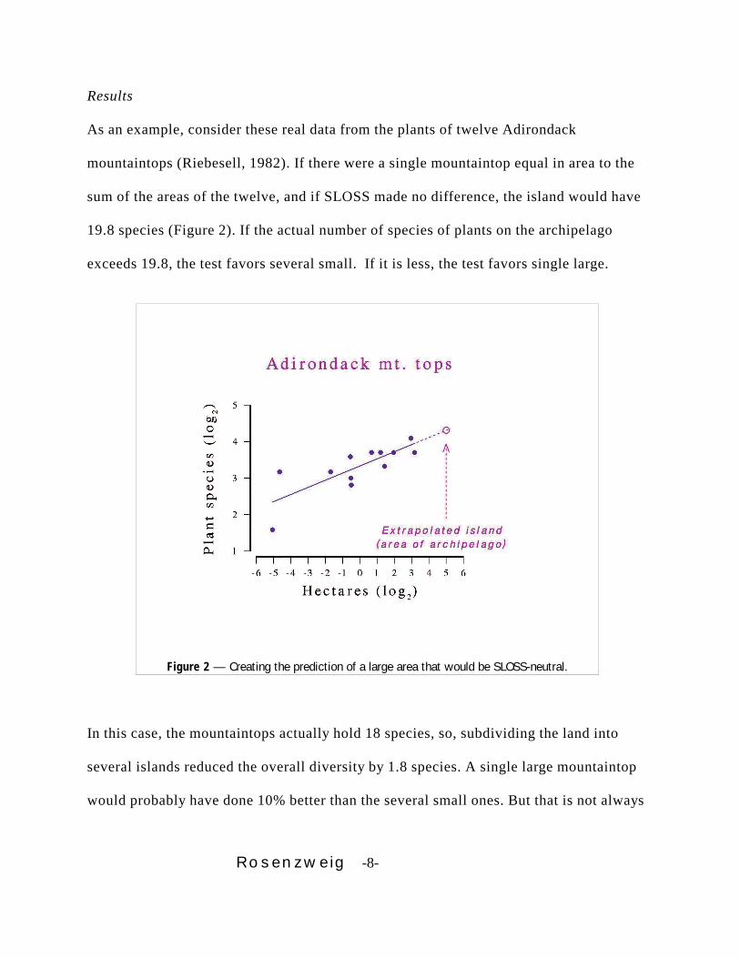
Figure 2 — Creating the prediction of a large area that would be SLOSS-neutral.

Results

As an example, consider these real data from the plants of twelve Adirondack

mountaintops (Riebesell, 1982). If there were a single mountaintop equal in area to the

sum of the areas of the twelve, and if SLOSS made no difference, the island would have

19.8 species (Figure 2). If the actual number of species of plants on the archipelago

exceeds 19.8, the test favors several small. If it is less, the test favors single large.

In this case, the mountaintops actually hold 18 species, so, subdividing the land into

several islands reduced the overall diversity by 1.8 species. A single large mountaintop

would probably have done 10% better than the several small ones. But that is not always

Rosenzweig -9-

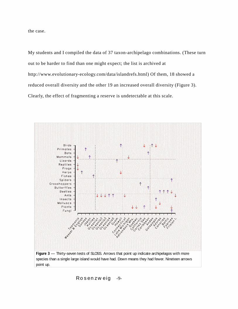
Figure 3 — Thirty-seven tests of SLOSS. Arrows that point up indicate archipelagos with morespecies than a single large island would have had. Down means they had fewer. Nineteen arrowspoint up.

the case.

My students and I compiled the data of 37 taxon-archipelago combinations. (These turn

out to be harder to find than one might expect; the list is archived at

http://www.evolutionary-ecology.com/data/islandrefs.html) Of them, 18 showed a

reduced overall diversity and the other 19 an increased overall diversity (Figure 3).

Clearly, the effect of fragmenting a reserve is undetectable at this scale.

Rosenzweig -10-

Whether reserves are ‘single-large’ or ‘several-small’ may well matter at very small

scales because of edge effects and population dynamics. And it surely matters at large

scales within a continent, because a single large reserve would reduce the variety of

habitats we set aside. But the evidence shows that at the medium spatial scales for

which it was conceived, SLOSS does not seem to matter at all. And it also should not

matter at the largest scale, the interprovincial, as we shall now see.

SPARs and the impact of exotic species

Some exotic species do considerable ecological damage (Mooney & Cleland, 2001).

This unassailable fact has led to the reification that exotic species are evil, that they

always and everywhere pose a threat to diversity (Slobodkin, 2001). But that is a leap

unsupported by our science (Sagoff, 1999). What can SPARs teach us about the true

nature of the threat vis-à-vis overall diversity?

The ultimate condition imagined by biogeographers is termed the New Pangaea (thanks

to Hal Mooney) or the Homogocene (thanks to Gordon Orians). Dispersal rates of

species among provinces are so high that their identity as separate provinces disappears.

Restricting ourselves to the earth’s land for purposes of illustration, we imagine a single

province, composed of all continents, whose area would be the sum of theirs.

Because they are close to linear, interprovincial SPARs predict that the New Pangaea

Rosenzweig -11-

Figure 4 — Plant diversities from both an intraprovincial SPAR andthe interprovincial one help to anchor the framework of SPARs thatpredict diversity in various sized provinces and portions of them.Because SPARs within different provinces are close to parallel, andNew Pangaea would have the greatest overall area, its pieces wouldhave higher diversity than those of smaller provinces.

will experience little or no decline in global steady-state diversities (Rosenzweig,

2001). For instance, if they are precisely linear, then the number of species in New

Pangaea will be the sum of the numbers of species in the old provinces. No gain, no

loss. Therefore, any reductions to global steady-state diversities caused by exotic

species will not last. That is not to say they will not happen; they already have. But they

will be temporary.

SPARs also predict that exotics will actually increase average local diversities at least

in the long term (Rosenzweig, 2001). Our idealized portrait of SPARs at various scales

shows this quite clearly. The SPAR that characterizes the New Pangaea will lie above

and be parallel to even the richest of the old provinces. So any piece of it will also be

Rosenzweig -12-

higher (Figure 4). Sax (xxxx) is showing that such increases are occurring already.

SPARs and indices of environmental status

Perhaps because concerns about our environment have grown, environmental indicators

have bred like rabbits. Each new question suggested a new indicator and made it seem

essential. In the mid-1990s, the US Environmental Protection Agency commissioned the

National Research Council to see whether it was possible to arrive at a very short list of

indicators that could be applied and compared broadly across the nation. The idea was

not to say that no other indicators might be useful in restricted circumstances. It was to

call for a meaningful, practical, uniform set to allow the country to assess its overall

environmental state, to give itself a sort of environmental report card.

Chaired by Gordon Orians and staffed by David Policansky, the NRC panel worked for

several years and the NRC issued its report (National Research Council, 2000). The

report arrives at a short list of indicators in which SPARs are featured prominently.

The NRC proposed that the ability of the land to support wild species amounts to a

powerful summary of its environmental status. But it recognized that simple counts of

the number of species are uninformative and unreliable. Simple counts are biased

! by sample size

! by the extent of the area in which they are measured: Larger areas have more

Rosenzweig -13-

species simply because they contain more habitats

! by the amount of time spent censusing them: More time leads to more species in

the raw count.

Simple counts also give no hint as to whether diversity is sustainable.

SPARs were the means recommended to deal with these shortcomings. Based on

SPARs, it set out three national diversity indicators:

1- Species Density: Because SPARs within a province are nonlinear, we cannot

rank areas, Ai, by their so-called ‘species densities’, Si/Ai. But we can adjust these raw

densities with the z-value of the species-area curve:

Di = Si/Aiz

Two areas with the same values of Di lie on the same SPAR and thus can be properly

considered to have the same species density.

2- Diversity Independence: Some species living in an area rely on other areas for

population support. SPAR allows us to estimate the proportion of such species in an

area.

3- Unnaturalness: Anthropogenic habitats often bring about the loss of many

Rosenzweig -14-

native species and the burgeoning of commensals, especially exotics. Recalculating Di

after excluding the commensal exotics produces a measure of the proportion of native

species expected at a site (of area A) but not found there.

High values of Di may reflect unsustainable, overloaded areas. In particular, if a high Di

is accompanied by a low independence score, we can expect the species density to

decline. SPARs can be used to estimate the likelihood and magnitude of decline.

The NRC shows how to use these diversity indicators to score land-use practices, too.

Combining these scores results in an index that can be interpreted as the national

environmental footprint and be monitored for signs of change.

SPARs and reducing the bias of sample size

Before the environmental indicators will do much good in practice, we must reduce the

amount of time and money it now takes to estimate diversity. This might also help to

reveal patterns of diversity that have eluded us so far because they exist at very fine

scales.

In fact, several statistical methods now allow fairly accurate estimation of diversity with

an order-of-magnitude reduction in the time and money it would otherwise take. Two of

the three most promising methods depend on extrapolating (to their asymptotes) SPARs

Rosenzweig -15-

taken at the point scale, i.e., generated by accumulating individuals in areas of fixed

heterogeneity.

For these purposes, one must work with plots of data that are arithmetic rather than

logarithmic. Using non-linear regression, we fit the coefficients of some general

formula to the species accumulation curve. The formula should rise with a negative

second derivative toward an asymptote. The asymptote is the estimate of how many

species are really in the system. The negative second derivative is required because all

real data sets rise that way. These formulae are not theories but merely templates like

the general linear equation, y = mx + b.

The Michaelis-Menten equation was the first extrapolation formula tried by an ecologist

(Holdridge et al., 1971):

(1)S S NN a

= + ,

where N is the number of individuals in the sample; a, the coefficient of curvature; S is

the asymptote (i.e., the true number of species in the system); and Sobs is the number of

species in the sample.

But the Michaelis-Menten equation fails to go through the point (1,1); instead it

Rosenzweig -16-

traverses the point (1,{S/1+a}). This is a defect because all samples of one individual

will contain one species.

One family of formulas that do go through the point (1,1), that may rise with a declining

slope, and that does converge on a positive asymptote is:

(2)S S N f N= − −1 ( )

,

where f(N) is any positive, unbounded, monotonically increasing function of N. As N

rises toward infinity, Eq.2 converges on S, the true diversity of the system.

We have worked with many such functions f(N) but two seem most promising.

Substituting them into eq. 2 produces the extrapolation estimators, formula 3 and

formula 5:

! Formula 3 uses f N q N( ) ln=

! Formula 5 uses f N qN q( ) =

In each case, q is a coefficient of curvature. (Formula numbers have no significance;

they are numbered arbitrarily according to the order in which we first used them to

attempt to improve Michaelis-Menten.) Both formulae (and many others) are available

in a PC application (Turner et al., 2000).

Rosenzweig -17-

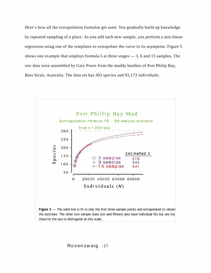
Figure 5 — The solid line is fit to only the first three sample points and extrapolated to obtainthe estimate. The other two sample sizes (six and fifteen) also have individual fits but are tooclose for the eye to distinguish at this scale.

Here’s how all the extrapolation formulae get used. You gradually build up knowledge

by repeated sampling of a place. As you add each new sample, you perform a non-linear

regression using one of the templates to extrapolate the curve to its asymptote. Figure 5

shows one example that employs formula 5 at three stages — 3, 6 and 15 samples. The

raw data were assembled by Gary Poore from the muddy benthos of Port Philip Bay,

Bass Strait, Australia. The data set has 303 species and 93,173 individuals.

Rosenzweig -18-

Figure 6a — Estimating diversity with the Michaelis-Menten formula. This shows thetypical negative bias retained with the method when it is given small sample sizes towork with.

We have tried the formulae on a variety of large data sets and found that the

extrapolation method works well. For consistency, I will again show a particular

example from the muddy benthos data set. I sampled it repeatedly and produced average

numbers of individuals and of species for each sample number. Diversity-in-hand rises

monotonically with a decelerating slope. In other words, the results become less and

less biased as sample size increases (Figure 6). That is precisely the point-scale SPAR.

Michaelis-Menten fits this SPAR very well (R2=0.9706) and formula 5 does even better

(R2=0.9997). But formula 5 does well even when sample sizes are far below 93,000. It

Rosenzweig -19-

Figure 6b — When given small sample sizes, formula 5 has a much smaller error andoften lies close to the horizontal, as in this case.

makes a reasonable estimate of diversity with only a few samples (Figure 6b). And, as

each new sample is added, its estimate of diversity changes only a little.

You can use these methods even if you have only presence/absence data from each

sample, and know nothing about abundances. You can even use them when you have yet

to sample all habitats of an area (in which case the increases in diversity are coming

from a combination of increasing sample size and real increase in diversity). To try this,

Rosenzweig et al. (2003) imagined a lepidopterist newly arrived in North America who

wanted to know how many species of butterfly live in the USA & Canada. By listing the

species in statistically dispersed sets of locales, the explorer could make a very good

Rosenzweig -20-

estimate (<10% error) even though she had listed only 11 of the continent’s 110

ecoregions. The median error was 2.4%.

SPARs and reconciliation ecology

Biogeographers and conservation biologists often use species-area relationships to

evaluate the future of species diversity. Biotic reserves are viewed as islands in a sea of

artificial, sterile habitats, so the patterns and theories of island biogeography are

applied. Among other things, island biogeography should tell us what proportion of

diversity these reserves ought to save (e.g., Brooks et al., 1997). A creative idea, but it

is far too optimistic.

Today’s reserves are not islands because they are usually all that remains to support so

much of life’s diversity. Islands, remember, get most of their species as immigrants

from a mainland source-pool. If a species now dependent upon our reserves were to

become extinct, it could not return from a source-pool. Species can get added only by

speciation. That means today’s system of reserves is more like a set of provinces than

anything else. That is a crucial distinction.

Because of the pronounced curvature of archipelagic SPARs — z-values are typically

about 0.3, you recall — islands do not have to be very large to contain a high percentage

of a source-pool’s species. For example, a single island with only 1% of the area of a

Rosenzweig -21-

source-pool can rather reliably harbor about 32% of its species. Given this power of

small islands, one can easily imagine that a set of island reserves could conserve most

of the species of the pool. However, they cannot if reserves are actually provinces.

Interprovincial SPARs have little or no curvature. Hence, a province reduced to 1% of

its former area can maintain only 1% of the old diversity; one reduced to 5%, can

maintain only 5% of the old diversity, etc. Our province-like system of reserves has lost

the economies of island biogeography.

Biogeography’s response to this quandary is crystal clear. If saving a small proportion

of surface area for diversity will not help very much, then get a larger proportion.

Obviously, that would seem to clash with another biological reality, Homo sapiens. I

won’t belabor the point.

But the previous paragraph conceals a tacit and false assumption, the assumption that

land use is a zero sum game, that the only way to make land available for wild species

is to exclude human beings and their works. Reconciliation ecology comes to say and to

show that this assumption is patently false. We can indeed get more land for other

species without putting it into reserves. Reconciliation ecology is the science of

inventing, establishing and maintaining new habitats to conserve species diversity in

places where people live, work or play (Rosenzweig, 2003).

Rosenzweig -22-

We already know that reconciliation ecology works. The pocket parks of Mayor Richard

Daley’s Chicago convert abandoned gas stations into islands of nature for inner city

residents. Prairie Dunes Country Club’s golf course in Hutchinson, Kansas hosts some

35,000 rounds of golf a year, but also manages its roughs to support a large number of

wild species (Terman). Florida Power and Light’s Turkey Point nuclear- and coal-

powered electricity generating station near Miami has 80 miles of cooling canals, canals

that it has made into crucial managed habitat for the rare American crocodile and many

other species (Gaby et al., 1985). And 20,000+ homeowners cooperate with the National

Wildlife Federation to build and manage a Backyard Habitat™ on their own property.

There are many, many more examples (http: //www.reconciliationecology.com). (See

also, McNeely (2002) for dozens of examples dealing with tropical agriculture.)

The point of this section, however, is to emphasize the science of reconciliation ecology

rather than to recite more cases of it. Although biogeography, through SPARs, gave

birth to reconciliation ecology, a lot of scientific parenting remains to be done. The

science will rarely be trivial. No scientific history convinces one of the difficulties

better than the reconciliation ecology of natterjack toads (Bufo calamita) in England

(Denton et al., 1997). It took some fifty scientists about a quarter of a century to bring

back this single species in this single place. Probably this amount of effort represents an

extreme, but we do not yet know.

Discussion

Rosenzweig -23-

As a group, the five SPAR applications hint at considerable opportunity for the

ecological biogeographer. Some of the applications are incomplete, some suggest

further basic research and some call for further applied research. I will explore these

points in this discussion.

Being able to reduce the biases of sampling promises value in several ways. We need to

do so to get more reliable data for our indicators. As the biases disappear from our

analyses, we will be able to acquire data at very fine scales. We can use them to search

for rapid changes in diversity and standing diversity patterns at fine scales of space and

time. I for one began worrying about these biases when I tried to estimate point

diversities: as space and time vanish, the inaccuracies introduced by sampling biases

become intolerable. They overwhelm the signal and lead to such nonsense as negative

diversity estimates.

Although we have a plethora of statistical tools for bias reduction, we are just learning

how to use them. The valuable methods of Lee and Chao (1994) seem to work well

within a fixed set of habitats. But they are not designed to handle data sets in which

habitat diversity and sample size increase together (Rosenzweig et al., 2003). They

break down under those conditions.

But why do we see variability in the accuracy of the extrapolation methods? How good

are they? Can we develop biologically meaningful estimates of confidence for them?

Rosenzweig -24-

(Those that now exist are confidence limits about the mean estimate — which includes

the error of bias — not about the true diversity.) Can we develop rules to teach us when

to stop sampling? Why does formula 5 with its single parameter of curvature seem to

outperform others with two? Does the design flaw in the Michaelis-Menten extrapolator

become unimportant when we use it on presence/absence data?

Those would seem to be a daunting list of questions and there are more. But it should

not take more than a few years to answer them. The software for experimenting with the

methods exists and makes the research practical (Turner et al., 2000). Meanwhile, the

methods already surpass the use of raw diversity data. We should use them — right

away! — albeit cautiously.

Biogeographers might also get involved in the work to collect and analyze data for the

indicators. In addition to those having to do with SPAR, others on the NRC short list

require the biogeographer’s touch. One of considerable importance, is a vector of land

use practices. Actually, it is more like a matrix, as each type of land use (e.g., farming)

has an orthogonal vector of treatments. All need to be measured using aerial

photography and satellite imagery. Then they need to be evaluated by looking at their

effects on life. This work, like painting the Golden Gate Bridge, will never end. So we

might as well get started.

In contrast, I believe the biogeographer’s work on exotic species is well in hand. I do

Rosenzweig -25-

find it ironic that the very concept of an exotic species is rooted in biogeography but

work on the problems associated with exotics (and they certainly exist) virtually ignored

biogeography for a long time. Nevermind. The price of errors got paid. It took

biogeography to fix them, after all. What remains is to discover why exotics have

sometimes enhanced local diversities and sometimes not. Will this be a permanent

difference or merely transitional? (Theory predicts the latter.)

And as far as I can tell, the SLOSS controversy is over. SLOSS does not matter.

Practically speaking, I am not sure it ever mattered much. Does any one know of an

actual situation in which someone used it (or tried to)? Its value was conceptual. It

planted the idea that biogeography might be used for conservation. Wilson and Willis

(1975) focused on loss of diversity as they set up the rest of their argument. On p.525

they wrote that they will apply “the quantitative theory of island biogeography” to “the

problems of diversity maintenance.” An inestimable breakthrough, really — as we see

now. That said, I cannot understand why the methods of biogeography were not quickly

used to resolve the question. In this chapter, I have done nothing about SLOSS that

could not have been accomplished in 1977 (with a few less data sets).

In contrast to SLOSS, reconciliation ecology is just beginning. And it overflows with

challenge and opportunity. Reconciliation ecology is nothing less than the deliberate

manipulation of species ranges. One begins by finding out what they are and what

makes them so. An immense amount of research lies ahead as we accumulate a library

Rosenzweig -26-

of the habitat requirements of myriad species, and learn how to combine them (National

Research Council, 2001). It will not be trivial to design landscapes of novel, diverse

habitats that support as many species as possible while also doing their jobs for people.

Will the bioinformatics of habitats addle the brains of those who are handling very well

the challenges of genetic informatics? And if that does not do it, what happens to them

when we admit that natural selection will alter habitat requirements simply because the

organisms will face new environments? I do not know that there has ever been a more

rigorous or exciting problem. Certainly, there has not been a more consequential one.

The path that leads to reconciled human habitats also calls for new attitudes and new

public and private institutions. But spawned and spurred on by biogeography,

reconciliation ecology addresses the new, sterile habitats in which most species cannot

function at all. If this new strategy of conservation biology spreads and influences a

substantial proportion of the earth’s area, it can halt the current mass extinction.

Who would have believed that a biogeographical pattern would lead to a vision of the

earth’s diversity in the far future? Who would have thought that it would offer

alternatives to civilization, allowing people to decide how much species diversity to

protect? Yet, these promises are contingent upon the next generation of biogeographers.

Will they pass the time debating the existence of the tool box? Or will they advance and

perfect the set of tools it contains? They must not shrug their shoulders in hopelessness

at the magnitude of the job or the callousness of the human psyche. Giving up would be

Rosenzweig -27-

a needless, terrible tragedy. The horse may need more training, but it can get us there.

Acknowledgements Gary Poore kindly allowed me to analyze his hard-won data. My

graduate class in species diversity of 2000 participated in the hunt for and analysis of

SLOSS-relevant data. Particular mention goes to Jessica Brownson, Zachary R Buchan,

John Cox, Daniel L Ginter, Martin Lingnau, Kevin Russell and Will Turner for their

efforts.

Rosenzweig -28-

References

Allen, A.P. & White, E.P. 2003. A unified theory for macroecology based on spatial

patterns of abundance. Evolutionary Ecology Research 5: 493–499.

Brooks, T.M., Pimm, S.L. & Collar, N.J. 1997. Deforestation predicts the number of

threatened birds in insular southeast Asia. Conservation Biology 11: 382-394.

Denton, J.S., Hitchings, S.P., Beebee, T.J.C. & Gent, A. 1997. A recovery program for

the natterjack toad (Bufo calamita) in Britain. Conservation Biology 11: 1329-

1338.

Gaby, R., McMahon, M.P., Mazzoti, F.J., Gillies, W.N. & Wilcox, J.R. 1985. Ecology

of a population of Crocodylus acutus at a power plant site in Florida. J.

Herpetology 19: 189-198.

Higgs, A.J. & Usher, M.B. 1980. Should nature reserves be large or small? Nature 285:

568-569.

Holdridge, L.R., Grenke, W.C., Hatheway, W.H., Liang, T. & Tosi, J.A. 1971. Forest

environments in tropical life zones. Oxford, UK: Pergamon Press.

Lee, S.-M. & Chao, A. 1994. Estimating population size via sample coverage for closed

capture-recapture models. Biometrics 50: 88-97.

Leitner, W.A. & Rosenzweig, M.L. 1997. Nested species-area curves and stochastic

sampling: a new theory. Oikos 79: 503-512.

McGill, B. & Collins, C. 2003. A unified theory for macroecology based on spatial

patterns of abundance. Evolutionary Ecology Research 5: 469–492.

Rosenzweig -29-

McNeely, J.A. & Scherr, S.J. 2002. Ecoagriculture: Strategies to Feed the World and

Save Wild Biodiversity. Washington, DC: Island Press.

Mooney, H.A. & Cleland, E.E. 2001. The evolutionary impact of invasive species. Proc.

National Academy of Sciences (USA) 98: 5446–5451.

National Research Council. 2000. Ecological Indicators For The Nation. Washington,

DC: National Academy Press.

National Research Council. 2001. Grand Challenges in Environmental Sciences.

Washington, DC: National Academy Press.

Quinn, J.F. & Harrison, S.P. 1988. Effects of habitat fragmentation and isolation on

species richness: evidence from biogeographic patterns. Oecologia 75: 132-140.

Riebesell, J.F. 1982. Arctic-alpine plants on mountaintops: agreement with island

biogeography theory. Amer. Natur. 119: 657-674.

Rosenzweig, M.L. 1995. Species Diversity in Space and Time. Cambridge, UK:

Cambridge University Press.

Rosenzweig, M.L. 1999. Species diversity. In Advanced Theoretical Ecology: principles

and applications (J. McGlade, ed), pp. 249-281. Oxford, UK: Blackwell

Science.

Rosenzweig, M.L. 2001. The four questions: What does the introduction of exotic

species do to diversity? Evol. Ecol. Research 3: 361-367.

Rosenzweig, M.L. 2003. Win-Win Ecology: How the Earth's Species Can Survive in the

Midst of Human Enterprise. New York: Oxford University Press.

Rosenzweig, M.L., Turner, W.R., Cox, J.G. & Ricketts, T.H. 2003. Estimating diversity

Rosenzweig -30-

in unsampled habitats of a biogeographical province. Conservation Biology 17:

864–874.

Sagoff, M. 1999. What's wrong with alien species? Report of the Institute for

Philosophy and Public Policy 19: 16–23.

Simberloff, D.S. & Abele, L.G. 1976. Island biogeography theory and conservation

practice. Science 191: 285--286.

Slobodkin, L.B. 2001. The good, the bad and the reified. Evolutionary Ecology

Research 3: 1–13.

Turner, W., Leitner, W.A. & Rosenzweig, M.L. 2000. Ws2m.exe.

http://eebweb.arizona.edu/diversity.

Wilson, E.O. & Willis, E.O. 1975. Applied biogeography. In Ecology and Evolution of

Communities (M.L. Cody & J.M. Diamond, ,eds), pp. 522-534. Cambridge,

Mass: Belknap Press of Harvard Univ. Press.