corel ventura - gec02 po - university of birminghamwbl/biblio/gecco2002/gecco-2002-14.pdf · along...

GENET IC PROGRAMMINGRiccardo Po l i , cha i r

A re-examination of the Cart Centering problem using the Chorussystem

R. Muhammad Atif Azad

Dept. of Computer Science

and Information Systems

University of Limerick

Ireland

[email protected]

Conor Ryan


and Information Systems


Ireland

[email protected]

Mark E. Burke

Dept. of Mathematics

and Statistics


Ireland

[email protected]

Ali R. Ansari

Dept. of Mathematics

and Statistics


Ireland

[email protected]

Abstract

The cart centering problem is well known in

the �eld of evolutionary algorithms and has

often been used as a proof of concept prob-

lem for techniques such as Genetic Program-

ming. This paper describes the application of

a grammar based, position independent en-

coding scheme, Chorus, to the problem. It

is shown that using the traditional experi-

mental setup employed to solve the problem,

Chorus is able to come up with the solutions

which appear to beat the theoretically opti-

mal solution, known and accepted for decades

in the �eld of control theory. However, fur-

ther investigation into the literature of the

relevant area reveals that there is an inher-

ent error in the standard E.C. experimental

approach to this problem, leaving room for a

multitude of solutions to outperform the ap-

parent best. This argument is validated by

the performance of Chorus, producing better

solutions at a number of occasions.

1 Introduction

The cart centering problem is a well known problem

that often appears in the introductory literature of op-

timal control (see [Athans, Falb, 66]). In its most basic

form, it involves a cart of massmmoving in one dimen-

sion on a frictionless horizontal surface. The cart can

be moving with any velocity v and can have any po-

sition x along the x-axis. The problem is to bring the

cart to the origin in a position-velocity space with the

values of both x and v approaching zero in minimum

amount of time. The literature shows that the prob-

lem already has a well de�ned solution, which guar-

antees that the cart is centered in minimum amount

of time. Genetic programming (GP) [Koza, 92] (pages

122 through 147) has been shown to have successfully

solved this problem. The experimental setup described

therein shows the absence of any success predicate,

meaning that the system is free to wander in the solu-

tion space and come up with anything that minimizes

the time required to center the cart.

This paper describes the application of a relatively

new, position independent, evolutionary automatic

programming system, Chorus [Ryan et al, 02a] on this

problem. The system involves a genotype pheno-

type distinction and like [Horner, 96], [Paterson, 97],

[Whigham, 95], and Grammatical Evolution (GE)

[Ryan, Collins, O'Neill, 98] [O'Neill, Ryan, 01] evolves

programs using grammars. While our aim initially for

this paper was to demonstrate that Chorus could be

successfully applied to the problem, we were surprised

to discover that our results showed that the system

produced expressions that were able to centre the cart

in less time compared to the theoretical optimal con-

trol strategy. However a closer examination of the

problem, as described in the control genre, re ects that

the approach traditionally employed to solve the prob-

lem involves an inherent error. As a result there is

no unique solution for this problem under the circum-

stances.

The paper �rst describes a context free grammar in

Backus Naur form, which is used to partially spec-

ify the behaviour of Chorus, similar to the way in

which one speci�es functions and terminals in GP.

We then describe the Chorus system and the process

involving the mapping from a genotype to phenotype

is discussed, with an example. Section 5 describes the

application of Chorus on the cart centering problem,

the theoretical background, the experimental setup

and then discusses the results in the light of literature

from control theory. Section 6 draws some conclusions

based on the experiences and results presented in the

paper.

GENETIC PROGRAMMING 707

2 Backus Naur Form

Backus Naur Form (BNF) is a notation for describ-

ing grammars. A grammar is represented by a tuple

fN;T; P; Sg, where T is a set of terminals, i.e. items

that can appear in legal sentences of the grammar, and

N is a set of non-terminals, which are interim items

used in the generation of terminals. P is the set of

production rules that map the non-terminals to the

terminals, and S is a start symbol, from which all le-

gal sentences may be generated.

Below is a sample grammar, which is similar to that

used by Koza [Koza, 92] in his symbolic regression and

integration problems. Although Koza did not employ

grammars, the terminals in this grammar are similar

to his function and terminal set.

S = <expr>

<expr> ::= <expr> <op> <expr> (0)

| ( <expr> <op> <expr>)(1)

| <pre-op> ( <expr> ) (2)

| <var> (3)

<op> ::= + (4) | - (5) | % (6)

| * (7)

<pre-op> ::= Sin (8) | Cos (9)

| Exp (A)| Log (B)

<var> ::= 1.0 (C) | X (D)

3 The Chorus System

Chorus[Ryan et al, 02a] is an automatic programming

system based coarsely on the manner in which en-

zymes regulate the model of a cell. Chorus belongs

to the same family of algorithms as Grammatical Evo-

lution [Ryan, Collins, O'Neill, 98] [O'Neill, Ryan, 01],

and shares several characteristics with it. In particu-

lar, the output of both systems is governed by a BNF

grammar as above, and the genomes, variable length

binary strings, interpreted as 8 bit integers (referred to

as codons), are used to produce legal sentances from

the grammar.

There is, however, a crucial di�erence. It concerns

the interpretation of each codon, which, when being

processed is moded with the total number of produc-

tion rules in the grammar. Thus each codon repre-

sents a particular production rule, regardless of its

position on the chromosome. This behaviour is dif-

ferent from GE, where an integer is moded with only

the number of rules that are relevant at that point in

time, and the meaning of a codon is determined by

those that precede it, leading to the so-called \ripple

e�ect"[Keijzer et al, 01].

For example, consider the individual:

18 28 32 27 42 17 18 31 27 14

45 46 45 18 27 55 65

which can be looked upon as a collection of hard coded

production rules. When moded with the number of

rules in the grammar (see section 2), which in this

case is 14, the same individual can now be represented

as follows (using hexadecimal numbers):

4 0 4 D 0 3 4 3 D 0

3 4 3 4 D D 9

Each gene encodes a protein which, in our case is a pro-

duction rule. Proteins in this case are enzymes that

regulate the metabolism of the cell. These proteins

can combine with other proteins (production rules in

our case) to take particular metabolic pathways, which

are, essentially, phenotypes. The more of a gene that

is present in the genome, the greater the concentra-

tion of the corresponding protein will be during the

mapping process [Zubay, 93] [Lewin, 99]. In a coarse

model of this, we introduce the notion of a concentra-

tion table. The concentration table is simply a mea-

sure of the concentrations of each of the proteins at any

given time, and is initialised with each concentration

at zero. At any stage, the protein with the greatest

concentration will be chosen, switching on the corre-

sponding metabolic pathway, thus, the switching on

of a metabolic pathway corresponds to the develop-

ment of the forming solution with the application of a

production rule.

Many decisions are made during the mapping process.

For example, the start symbol <expr> has four possi-

ble mappings. When such a situation occurs, the rel-

evant area from the concentration table is consulted

and the rule with the maximum concentration is cho-

sen. In case there is a tie, or the concentrations of all

the rules are zero, the genotype is searched for any of

the applicable rules, until a clear winner is found. This

is analogous to the scenario where there are a number

of voices striving for attention, and only the loudest is

heard.

While searching for an applicable production rule, one

may encounter rules that are not relevant at that point

in time. In this case, the concentrations of those rules

are increased, so when that production rule is involved

in a decision, it will be more likely to win. This is what

brings position independence into the system; the cru-

cial thing is the presence or absence of a gene, while

its position is less so. Importantly, absolute position

almost never matters, while occasionally, relative po-

sition (to another gene) is important.

GENETIC PROGRAMMING708

Once chosen, the concentration of that production rule

is decremented. However, it is not possible for a con-

centration to fall below zero.

Sticking to the left most non-terminal in the current

sentence, mapping continues until there are none left

or we are involved in a choice for which there is no

concentration either in the table or the genome. An

incompletely mapped individual is given a �tness value

of exactly zero in the current version of Chorus, thus

removing its chances of indulging into any reproduc-

tive activity.

3.1 Example Individual

Using the grammar from section 2 we will now demon-

strate the genotype-phenotype mapping of a Chorus

individual. The particular individual is encoded by

the following genome:

18 28 32 27 42 17 18 31 27 14

45 46 45 18 27 55 65

For clarity, we also show the normalised values of each

gene, that is, the genes mod 14. This is only done

for readability, as in the Chorus system, the genome is

only read on demand, and not decoded until needed.

4 0 4 D 0 3 4 3 D 0

3 4 3 4 D D 9

The �rst step in decoding the individual is the creation

of the concentration table. There is one entry for each

production rule (0..D), each of which is initially zero.

The table is split across two lines to aid readability.

Rule # 0 1 2 3 4 5 6

Concentration

Rule # 7 8 9 A B C D

Concentration

The sentence starts as <expr>, so the �rst choice must

be made from productions 0..3, that is:

<expr> ::= <expr> <op> <expr> (0)

| ( <expr> <op> <expr>)(1)

| <pre-op> ( <expr> ) (2)

| <var> (3)

None of these have a value yet, so we must read the

�rst gene from the genome, which will cause it to pro-

duce its protein. This gene decodes to 4, which is not

involved in the current choice. The concentration of 4

is incremented, and another gene read. The next gene

is 0, and this is involved in the current choice. Its con-

centration is amended, and the choice made. As this

is the only relevant rule with a positive concentration,

it is chosen and its concentration is reduced, and the

current expression becomes:

<expr><op><expr>

The process is repeated for the next leftmost non-

terminal, which is another expr. In this case, again the

concentrations are at their minimal level for the pos-

sible choices, so another gene is read and processed.

This gene is 4, which is not involved in the current

choice, so we move on and keep reading the genome till

we �nd rule 0 which is a relevant rule. Meanwhile we

increment the concentrations of rule 4 and D. Similar

to the previous step, production rule #0 is is chosen,

so the expression is now

<expr><op><expr><op><expr>

Reading the genome once more for the non-terminal

expr, produces rule 3 so the expression becomes

<var><op><expr><op><expr>

The state of the concentration table at the moment is

given below.

Rule # 0 1 2 3 4 5 6

Concentration 2


Concentration 1

The next choice is between rules #C and #D, however,

as at least one of these already has a concentration,

the system does not read any more genes from the

chromosome, and instead uses the values present. As

a result, rule <var> -> X is chosen to introduce �rst

terminal symbol in the expression.

Once this non-terminal has been mapped to a termi-

nal, we move to the next left most terminal, <op> and

carry on from there. If, while reading the genome, we

come to the end, and there is still a tie between 2 or

more rules, the one that appears �rst in the concen-

tration table is chosen. However if concentrations of

all the relevant rules is zero, the mapping terminates

and the individual responsible is given a suitably chas-

tening �tness.

With this particular individual, mapping continues

until the individual is completely mapped. The in-

terim choices made by the system are in the order:

4; 3; D; 4; 0; 3; D; 4; 3; D. The mapped individual is

X + X + X + X

The state of the concentration table at the end of the

mapping is given in the next table.

Notice that there are still some concentrations left in

the table. These are simply ignored in the mapping


Rule # 0 1 2 3 4 5 6

Concentration 2


Concentration

process and, in the current version of Chorus, are not

used again. Notice also that the rule #9 is not read

because the mapping terminates before reading this

codon.

4 Genetic Operators

The binary string representation of individuals e�ec-

tively provides a separation of search and solution

spaces. This permits us to use all the standard genetic

operators at the string level. Crossover is implemented

as a simple, one point a�air, the only restriction be-

ing that it takes place at the codon boundaries. This

is to permit the system to perform crossover on well-

formed structures, which promotes the possibility of

using schema analysis to examine the propagation of

building blocks. Unrestricted crossover will not harm

the system, merely make this kind of analysis more

diÆcult.

Mutation is implemented in the normal fashion, with a

rate of 0.01, with crossover occuring with a probability

of 0.9. Steady state replacement is used, with roulette

wheel selection.

As with GE, if an individual fails to map after a com-

plete run through the genome, wrapping operator is

used to reuse the genetic material. However, the exact

implemenation of this operator has been kept di�er-

ent. Repeated reuse of the same genetic material e�ec-

tively makes a wrapped individual behave like multiple

copies of the same genetic material stacked on top of

each other in layers. When such an individual is sub-

jected to crossover, the stack is broken into two pieces.

When linearized, the resultant of crossover is di�erent

from one or the other parent at regular intervals. In or-

der to minimize such happenings, the use of wrapping

has been limited to initial generation. After wrapping,

the individual is attened or unrolled, by putting all

the layers of the stack together in a linear form. The

unrolled individual then replaces the original individ-

ual in the population. This altered use of wrapping

in combination with position exibility, promises to

maintain the exploitative e�ects of crossover. Unlike

GE, the individuals that fail to map on the second

and subsequent generations are not wrapped, and are

simply considered infeasible individuals.

5 The Cart Centering Problem

The cart centering problem is well known in the area

of evolutionary computation. Koza[Koza, 92] success-

fully applied GP to it, to show that GP was able to

come up with a controller that would center the cart

in the minimum amount of time possible.

The problem, also referred to as the double integrator

problem, appears in introductory optimal control text-

books as the classic application of Pontryagin's Prin-

ciple (see for instance [Athans, Falb, 66]). There has

been considerable research conducted into the theo-

retical background of the problem, and the theoreti-

cal best performance can be calculated, even though

designing an expression to produce this performance

remains a non-trivial activity.

As Evolutionary Computation methods are bottom up

methods, they do not, as such, adhere to problem spe-

ci�c (be it theoretic or practical) information. This

means that E.C. can be used as a testing ground for

theories - if one can break the barriers proposed by

theoreticians, then it probably means that there is a

aw in the theory concerned. However, another possi-

bility is that there is a aw in the experimental set up,

that makes it appear as though the theoretical best

has been surpassed.

This section describes the application of Chorus to the

cart centering problem, an exercise which ppears to

consistently produce individuals that surpass the the-

oretical best, before discussing the implications of the

result.

5.1 Theoretical Background

In its most basic form, we consider a \cart" as a parti-

cle of massmmoving in one dimension with position at

time t of x(t) relative to the origin, and corresponding

velocity v(t). The cart is controlled by an amplitude

constrained thrust force u(t); ju(t)j � 1, and the con-

trol objective is to bring the cart to rest at the origin

in minimum time on a frictionless track. The state

equations are

dx

dt= v

dv

dt=

1

mu

or

d

dt

�x

v

�=

�0 1

0 0

��x

v

�+

�0

1=m

�u (1)

The solution is a unique \Bang-Bang " control (u(t)

takes only the values +1 or -1) with at most 1 switch


which is expressible in feedback form (u = u�(x; v))

in terms of a \switching curve" S in the x � v plane.

Following the approach of [Athans, Falb, 66] we �nd

that S is given by

x+m

2vjvj = 0; (2)

the optimal control by

u� =

8<:

�1; if x+ m

2vjvj > 0

+1; if x+ m

2vjvj < 0

�v=jvj; if x+ m

2vjvj = 0

(3)

and the minimum time T to reach (0; 0) from (x; v) by

T =

8<:

mv +p2m2v2 + 4mx; if x+ m

2vjvj > 0

�mv +p2m2v2 � 4mx; if x+ m

2vjvj < 0

mjvj; if x+ m

2vjvj = 0

(4)

The above formulae assume that the system can switch

precisely when condition (2) is met. In practice, this

is only approximated. The engineering literature con-

tains analyses of what happens when non-ideal switch-

ing (deadband and/or hysteresis) occurs using real

hardware with the resultant cycling, chattering and

steady state error. (see [Gibson, 63] for more details).

5.2 Experimental Setup

GP has been shown to be able to successfully evolve

the time optimal control strategy (see [Koza, 92]). The

same experimental setup is used by Chorus except

where mentioned otherwise. The simulation essen-

tially entails a discretisation of the problem so as to

enable a numerical approximation of the derivatives in-

volved. This is referred to as an Euler approximation

of the di�erential equations given in (1), i.e.,

x(t+ h) = x(t) + hv(t);

v(t+ h) = v(t) +h

mu(t);

where m is the mass of the cart, h represents the time

step size, v(t+ h) and x(t+ h) represent velocity and

distance from the origin respectively at time t+h and

v(t) and x(t) represent velocity and distance from the

origin respectively at time t. The desired control strat-

egy should satisfy the following conditions.

It should specify the direction of the force to be

applied for any given values of x(t) and v(t).

The cart approximately comes to rest at the ori-

gin, i.e., the Euclidean (x; v) distance from the

origin is less than a certain threshold.

The time required is minimal.

The exact time optimal solution is characterised by

the switching condition

�x(t) > v2(t)Sign v(t)

2jumaxj=m ; (5)

which applies the force in the positive x direction if the

above condition is met and in the negative direction

otherwise. Note that umax represents the maximum

value of u(t), which is 1 here. The Sign function re-

turns +1 for a positive argument and -1 otherwise. For

the sake of simplicity m is considered to be equal to

2.0 kilograms and the magnitude of the force u(t) is

1.0 Newtons, so that the denominator equals 1.0 and

can be ignored. The experimental settings employed

by Koza are summarised in table 1. Note that (5)

does not incorporate the equality condition mentioned

in (3).

Table 1: A Koza-style Tableau For The Cart Centering

Problem.

Objective: Find a time optimal bang-bangcontrol strategy to center a cart on aone dimensional frictionless track.

Terminal Set: The state variables of the system:x (position of the cart along Xaxis), v (velocity V of the cart)and -1.0.

Function Set: +,-,*,%,ABS,GT.Fitness cases: 20 initial condition points (x; v)

for position and velocity chosenrandomly from the square inposition-velocity space havingopposite corners, (�0:75; 0:75)and (0:75;�0:75).

Fitness: Reciprocal of sum of the time, over20 �tness cases, taken to center thecart. When a �tness case times out,the contribution to the sum is 10.0seconds.

Hits: Number of �tness cases that didnot time out.

Wrapper: Converts any positive valuereturned by an expression to +1 andconverts all other values(negative or zero) to -1.

Parameters: M = 500, G = 75Success Predicate: None.

The grammar used for the problem is:

S = <expr>

<expr> ::= <expr> <op> <expr>

| ( <expr> <op> <expr>)


| <pre-op> ( <expr> )

| <var>

<op> ::= + | - | % | * | GT

<pre-op> ::= ABS

<var> ::= X | V | -1.0

The randomly generated 20 �tness cases used by Cho-

rus are given in the table 2.

Table 2: Randomly Generated 20 Starting Points,

given as ((x; v) pairs).

0.50,0.67 -0.65,0.40 -0.16,-0.57 0.10,0.50

-0.71,0.66 0.43,0.01 -0.28,-0.71 0.27,-0.73

-0.50,0.34 -0.57,0.32 0.43,-0.69 -0.52,-0.16

-0.33,-0.21 -0.16,-0.06 0.71,-0.69 -0.04,-0.63

0.39,0.70 -0.52,-0.42 -0.59,0.38 0.58,-0.35

The cart is considered to be centered if the Euclidean

distance from the origin (0; 0) is less than or equal to

0.01. The total time taken by the strategy (5) over all

the given set of starting points is 56.07996 seconds. On

average it takes 2.803998 seconds per �tness case for

the cart to be centered. This means that any strategy

which centers the cart in less time, does better than

the theoretical solution (5) for this experimental setup.

5.3 Experimental Results

The work of Koza [Koza, 92] shows that the optimal

control strategy can be evolved using GP. However,

it has not been shown that even in the absence of

any success predicate, any strategy was evolved which

could beat the result as described by the inequality

(5). When the same task is given to the Chorus sys-

tem, 17 times out of 20 independent runs, it evolves

what appears to be a better strategy in terms of time

minimisation. Out of those 17 runs, on the average,

a better strategy is produced in the 39th generation,

the earliest being 20th and the latest being 65th.

One of the samples which broke the barrier is given as

(�1:0 �X) GT (V �ABS(V ) + V � V � V );

which can be rewritten as

�x(t) > v2(t)Sign v(t) + v

3(t); (6)

returning +1 if the condition is satis�ed and �1 oth-

erwise. Total time recorded for this control law men-

tioned by inequality (6) is 50.799965 seconds over 20

�tness cases which is clearly less than the solution

shown by the inequality (5). However, the least time

that was recorded was 49.919968 seconds. A plot of x

versus v for the control strategy given in (5) is shown

in Fig 1(a) for the starting point (0:50; 0:67). A simi-

lar plot for the strategy evolved by the Chorus system

is shown in Fig 1(b). Notice that in (a) the control

strategy crosses the y-axis leading into the negative

x-axis region and then it returns to the origin. This

shows the longer route traversed by (a) compared to

(b) where there is no such occurrence, thus re ecting

the time di�erence between the two strategies.

(a)x

v

-0.8

-0.6

-0.4

-0.2

0

0.2

0.4

0.6

0.8

-1 -0.5 0 0.5 1

(b)x

v

-0.8

-0.6

-0.4

-0.2

0

0.2

0.4

0.6

0.8

-1 -0.5 0 0.5 1

Figure 1: .Trajectories traversed by the two strategies

to reach the origin. (a) represents inequality (5) and

(b) represents the evolved strategy (6)

5.4 Discussion

It appears from the results in the previous section

that a solution better than the theoretical has been

achieved. However, a careful consideration of the

problem undertaken shows otherwise. This problem

has been solved by �rst discretising the main di�eren-

tial equations as mentioned earlier. The discretisation

brings with it an element of error. The time step h


used now plays a major role, in the sense that a smaller

time step would lead to a better solution i.e., closer to

the theoretical solution (3), and as h! 0 the solution

converges to (3).

The time step employed by Koza [Koza, 92] is h =

0:02, and using this time step, the error in the deriva-

tives is substantial enough to cause the systems to con-

verge to control laws other than the theoretical result

in (3). In this sense Chorus actually validates this by

evolving to what is a better solution than (5).

A study of the appropriate literature in the control

theory genre indicates that the theoretical model is

just that, theoretical. Practical implementation of a

control system which brings the cart to the target po-

sition is not even \bang-bang" (i.e u(t) is either +1 or

-1). Instead, the magnitude of the applied force is any

real number between 0 and 1.

One approach is to model the situation as one in which

the control can change only at discrete-time steps, ei-

ther as a sampled data system or a discretised version

of eq(1). The former leads to state equations

x(t + h) = x(t) + Æv(t) +Æ2

2mu(t)

v(t+ h) = v(t) +Æ

mu(t)

where 1=Æ is the sampling rate. The latter, using an

Euler discretisation scheme, leads to state equations

x(t+ h) = x(t) + hv(t)

v(t+ h) = v(t) +h

mu(t)

where h is the step size.

When Æ = h, both models are of the form

�x(t+ h)

v(t+ h)

�=

�1 h

0 1

��x(t)

v(t)

�+

�b

h=m

�u(t)

(7)

where b = h2=2m for the sampled data model and

b = 0 for the discretised model.

The control objective is again to bring the state of eq

(7) to the origin in minimum time using a sequence of

amplitude constrained controls juj � 1. However, due

to the discrete time steps, the solution of the problem

is fundamentally di�erent to that of the continuous

time problem of (1). The optimal control is in general

no longer unique, nor except for a set of isolated points

in the x� v plane is it Bang-Bang throughout. Hence

there are di�erent approaches and algorithms.

The more general problem in n dimensions was

initially formulated in [Kalman, 57], and then

analysed comprehensively in [Desoer, Wing, 61a] -

[Desoer, Wing, 61c]. This analysis, when applied to

the cart centering problem recursively constructs a se-

quence of convex sets fCkg, where Ck is the set of

states for which there exists an admissible input se-

quence which transfers the state to the origin in k time

steps but no fewer (C0 = f(0; 0)g). For instance, if wewant to centre the cart in 1 time step then C1 rep-

resents the region of interest. For any (x1; v1) 2 C1,

the cart is guaranteed to be centered in exactly 1 time

step. In addition, a piecewise linear switching curve

is constructed which divides the plane into regions of

positive and negative control values (see �gure 2).

x

v

Figure 2: The sets C1 - C8 for the Euler discretised

system with a cart of mass m = 2 and h = 0:02

Later work has looked at describing the Ck in

terms of their facets with associated algorithms

[Keerthi, Gilbert, 87], and there is still much interest

in improving the eÆciency of the existing algorithms

(see [Jamak, 00] for a good review).

6 Conclusions

We have described the application of a position inde-

pendent, representation scheme for Evolutionary Algo-

rithms, termed Chorus, on the cart centering problem.

Much to our surprise, Chorus apparently succeeded in

producing individuals that performed better than the

theoretical best. However, further analysis of the prob-

lem and traditional experimental set up revealed aws

that changed the nature of the problem.


The paper describes how Chorus was able to exploit

these aws to produce surprisingly �t individuals, and

how an Evolutionary Computation system can be used

to help test models of physical systems. Also, it re-

emphasizes the point that while attempting to solve

continuous problems numerically, we should be ware

of the resultant discretisation errors. It is also worth

noting that the way these problems are typically solved

by control engineers is by starting with the discretised

analogues of the continuous problems and then pro-

ceeding to solve. It might be worth exploring what a

system like Chorus may have to o�er in the solution

process of such a discretised problem.

6.1 Future Work

The results shown in the cart centering problem en-

courage the use of Chorus for real world problems.

Coupled with the strengths of the system discussed in

[Ryan et al, 02a], the system can be applied but not

limited to the problems in the �eld of control theory

and uid dynamics.

Chorus diverges considerably from algorithms in the

same \family", e.g. Grammatical Evolution and

GAUGE[Ryan et al, 02b] in that it does not exploit

the ripple e�ect, and instead uses position indepen-

dent, absolute genes. This makes Chorus very suit-

able for schema analysis, and also possible that the

Genetic Algorithm Schema Theory could, with very

little extension, be applied to an automatic program-

ming system.

References

[Athans, Falb, 66] Athans M. and P. L. Falb, Optimal

Control, McGraw-Hill, 1966.

[Desoer, Wing, 61a] Desoer C.A. and J. Wing, \An

Optimal Strategy for a Saturating

Sampled-Data System", IRE Transactions

on Automatic Control, vol AC-6, pp. 5-15,

1961.

[Desoer, Wing, 61b] Desoer C.A. and J. Wing, \A

Minimal Time Discrete System", IRE

Transactions on Automatic Control, vol

AC-6, pp. 111-125, 1961.

[Desoer, Wing, 61c] Desoer C.A. and J. Wing, \Min-

imal Time Regulator Problem for Linear

Sampled-Data Systems (General Theory)",

J. Franklin Inst., vol 20, pp. 208-228, 1961.

[Gibson, 63] Gibson J.E., Nonlinear Automatic Con-

trol, McGraw-Hill, 1963.

[Goldberg, Korb, Deb, 89] Goldberg D E, Korb B,

Deb K. Messy genetic algorithms: motiva-

tion, analysis, and �rst results.

Complex Syst. 3

[Horner, 96] H. Horner, A C++ class library for Ge-

netic Programming: The Vienna Univer-

sity of Economics Genetic Programming

Kernel. Release 1.0, Operating instruction.

Vienna University of Economics, 1996.

[Jamak, 00] Jamak A., \Stabilization of Discrete-

Time Systems with Bounded Control In-

put", MASc Dissertation, University of

Waterloo, Waterloo CA.,2000.

[Kalman, 57] Kalman, R.E., \Optimal Nonlinear

Control of Saturating Systems by Intermit-

tent Action" , 1957 IRE Wescon Conven-

tion Record, pt 4, pp 130-135.

[Keerthi, Gilbert, 87] Keerthi S.S. and E.G. Gilbert,

\Computation of Minimum-Time Feedback

Control Laws for Discrete-Time Systems

with State-Control Constraints", IEEE

Transactions on Automatic Control, vol

AC-32, pp. 432-435, 1987.

[Keijzer et al, 01] Keijzer M., Ryan C., O'Neill M.,

Cattolico M., Babovic V. Ripple Crossover

In Genetic Programming, in Proceedings of

EuroGP'2001.

[Koza, 92] J. Koza. \Genetic Programming". MIT

Press, 1992.

[Lewin, 99] Lewin B. Genes VII. Oxford University

Press, 1999.

[O'Neill, Ryan, 01] O'Neill M., Ryan C. Grammati-

cal Evolution. IEEE Transactions on Evo-

lutionary Computation. 2001.

[Paterson, 97] N. Paterson and M. Livesey, \Evolv-

ing caching algorithms in C by GP" in Ge-

netic Programming 1997: Proc. 2nd Annu.

Conf., MIT Press, 1997, pp. 262-267. MIT

Press.

[Ryan, Collins, O'Neill, 98] C. Ryan, J.J. Collins

and M. O'Neill, \Grammatical Evolution:

Evolving Programs for an Arbitrary Lan-

guage", in EuroGP'98: Proc. of the First

European Workshop on Genetic Program-

ming (Lecture Notes in Computer Science

1391), Paris, France: Springer 1998, pp. 83-

95.


[Ryan et al, 02a] C. Ryan, A. Azad, A. Sheahan and

M. O'Neill, \No Coercion and No Pro-

hibition, A Position Independent Encod-

ing Scheme for Evolutionary Algorithms -

The Chorus System". In the Proceedings of

European Conference on Genetic Program-

ming (EuroGP 2002).

[Ryan et al, 02b] C. Ryan, Miguel Nicolau, and M.

O'Neill, \Genetic Algorithms Using Gram-

matical Evolution". In the Proceedings of

European Conference on Genetic Program-

ming (EuroGP 2002).

[Whigham, 95] P. Whigham, \Grammatically-based

Genetic Programming" in Proceedings of

the Workshop on GP: From Theory to Real-

World Applications, Morgan Kaufmann,

1995, pp. 33-41.

[Zubay, 93] Zubay G. Biochemistry. Wm. C. Brown

Publishers, 1993


A Survey and Analysis of Diversity Measures in GeneticProgramming

Edmund Burke Steven Gustafsony

School of Computer Science & ITUniversity of NottinghamNottingham, UK NG81BB

fekb j smg j [email protected] author

Graham Kendall

Abstract

This paper presents a survey and comparisonof the signi�cant diversity measures in thegenetic programming literature. The over-all aim and motivation behind this study isto attempt to gain a deeper understandingof genetic programming dynamics and theconditions under which genetic programmingworks well. Three benchmark problems (Ar-ti�cial Ant, Symbolic Regression and Even-5-parity) are used to illustrate di�erent di-versity measures and to analyse their corre-lation with performance. The results showthat diversity is not an absolute indicator ofperformance and that phenotypic measuresappear superior to genotypic ones. Finallywe conclude that interesting potential existswith tracking ancestral lineages.

1 INTRODUCTION

Maintaining population diversity in genetic program-ming (Banzhaf et al., 1998) is referred to as the keyin preventing premature convergence and stagnationin local optima (McPhee and Hopper, 1999)(Ryan,1994)(Ek�art and N�emeth, 2000)(McKay, 2000)(Rosca,1995a). Diversity is the amount of variety in the pop-ulation de�ned by what genetic programming indi-viduals `look' like or how they `perform'. The num-ber of di�erent �tness values (phenotypes) (Rosca,1995b), di�erent structural individuals (genotypes)(Langdon, 1996), edit distances between individuals(Ek�art and N�emeth, 2000), and complex and com-posite measures (McKay and Abbass, 2001)(Keijzer,1996)(D'haeseleer, 1994) are used as measures of di-versity. At the individual level, diversity measures dif-ferences between individuals and is used to select in-

dividuals for reproduction or replacement (Eshelmanand Scha�er, 1993).

In this study, we examine the previous uses and mean-ings of diversity, compare these di�erent measures onthree benchmark problems and discuss the results. Asfar as the authors are aware, all the signi�cant diver-sity measures that occur in the genetic programmingliterature are reported.

The ultimate goal is to determine a good measurementof population diversity and understand the e�ects ofits in uence as the evolutionary search progresses. Theoverall motivation of this study is that a better under-standing of diversity and diversity measures will leadto a better understanding of genetic programming andthe advantages and disadvantages of employing it inany given situation.

The following sections examine di�erent measures ofdiversity, how these measures relate to each other andhow they relate to the performance of three geneticprogramming problems. Section 2 describes measuresof population diversity and previous methods of pro-

moting diversity in populations. Section 3 describesthe experiments. Section 4 presents and discuss re-sults. Section 5 draws some brief conclusions and Sec-

tion 6 outlines some ideas for future work.

2 DIVERSITY MEASURES

Some measures of diversity are intended to quantifythe variety in a population and others are used tomeasure the di�erence between individuals. The lat-ter type is used to attempt to control or promote highdiversity during a run. The following section surveysboth measures that provide a quanti�cation of popu-lation diversity and methods used to actively promoteand maintain diversity within genetic programming.


2.1 POPULATION MEASURES

The most common type of diversity measure is that ofstructural di�erences between programs. Koza (1992)used the term variety to indicate the number of di�er-ent programs his populations contained. In this mea-sure, two programs are structurally compared, lookingfor exact matches. Landgon (1996) felt that genotypicdiversity was a suÆcient upper bound of populationdiversity as a decrease in unique individuals must alsomean a decrease in unique �tness values. More com-plex genotype measures count subtrees, size, and typeand frequencies of nodes.

Keijzer (1996) measures program variety by the num-ber of unique individuals and subtree variety by count-ing unique subtrees. Population diversity is a ratio ofthe number of unique individuals over population sizeand subtree variety is the ratio of unique subtrees overtotal subtrees. Tackett (1994) also measures struc-tural diversity using unique subtrees and schemata fre-quencies. D'haeseleer and Bluming (1994) de�ne thefrequency of terminals and functions as \genotypicaldiversity" and �tness case results as \phenotypical di-versity", which are correlated within the populationfor their study of local populations and demes.

When tree representations of genetic programs areconsidered as graphs, individuals can be compared forisomorphism (Rosca, 1995a) to obtain a more accuratemeasure of diversity. Determining graph isomorphism,however, is computationally expensive for an entirepopulation. We could count the number of nodes, ter-minals, functions and other graph properties in a rea-sonable time and use this n-tuple to determine whethertrees are possible isomorphs of each other.

McPhee and Hopper (1999) investigate diversity at thegenetic level by tagging each node created in the initialgeneration with a unique id. Root parents, the par-ents whose tree has a portion of another individual'ssubtree swapped into it during crossover, are assignednew memids, an auxiliary tag that is initially the samevalue of the id. All the nodes from the root down tothe crossover point are assigned new memids to indi-cate that these nodes have one new child. If there isno mutation in the genetic programming system (ashere), then no new ids will be created after the initialgeneration, only memids. McPhee and Hopper foundthat the number of unique ids dramatically falls afterinitial generations and, by tracking the root parents,after an average of 16 generations, all further individ-uals have the same common root ancestor.

Phenotypic measures compare the number of unique�tness values in a population. When the genetic pro-

gramming search is compared to traversing a �tnesslandscape, this measure provides an intuitive way tothink of how the population covers that landscape.Other measures could be created by using �tness val-ues of a population, as done by Rosca (1995a) withentropy and free energy. Entropy here representsthe amount of disorder of the population, where anincrease in entropy represents an increase in diver-sity. Bersano-Begey (1997) track how many individu-als solve which �tness cases. By monitoring the pop-ulation, a pressure is added to individuals to promotethe discovery of di�erent or less popular solutions.

2.2 PROMOTING DIVERSITY

Several measures and methods have been used to pro-mote diversity by measuring the di�erence between in-dividuals. These methods typically use a non-standardselection, mating, or replacement strategy to bol-ster diversity. Neighborhoods, islands, niches, crowd-ing and sharing from genetic algorithms are commonthemes to these methods.

Eschelman and Scha�er (1993) use Hamming distancesbetween individuals to select individuals for recombi-nation and replacement to improve over hill-climbing-type selection strategies for genetic algorithms.

Ryan's (1994) \Pygmie" algorithm builds two listsbased on �tness and length to facilitate selection forreproduction. The algorithm maintains more diver-sity and prevents premature convergence. The advan-tage of this algorithm is that it does not attempt to\over-control" evolution and uses simple measures topromote diversity.

De Jong et al (2001) use multiobjective optimisa-tion to promote diversity and concentrate on non-dominated individuals according to a 3-tuple of<�tness,size,diversity>. Diversity is the averagesquare distance to other members of the population,using a specialised measure of edit distance betweennodes. This multiobjective method promotes smallerand more diverse trees.

McKay (2000) applies the traditional �tness sharing

concept from Deb and Goldberg (1989) to test its fea-sibility in genetic programming. Diversity is the num-ber of �tness cases found, and the sharing concept as-signs a �tness based on an individual's performancedivided by the number of other individuals with thesame performance. McKay also studies negative corre-lation and a root quartic negative correlation in (2001)to preserve diversity. Ek�art and N�emeth (2000) apply�tness sharing with a novel tree distance de�nition andsuggest that it may be an eÆcient measure of struc-


tural diversity.

By surveying previous work using diversity measures,we designed several experiments to determine relation-ships between di�erent population measures of diver-sity and how they correlate to the best �tness of arun.

3 EXPERIMENTS

In this study we would like to answer two questions:One, how do di�erent measures of diversity relate toeach other, and two, how do those measures correlateto the best �tness of a run. Three common problemsare used with common parameter values from previousstudies. For all problems, a population size of 500 in-dividuals, a maximum depth of 10 for each individual,a maximum depth of 4 for the tree generation half-n-half algorithm and internal node selection probabilityof 0.9 for crossover is used. Additionally, each runconsists of 51 generations, or until the ideal �tness isfound.

The Arti�cial Ant, Regression and Even-5-Parityproblems are used. All three problems are typical togenetic programming and can be found in many stud-ies, including (Koza, 1992). The ant problem is con-cerned with �nding the best strategy for picking uppellets along a trail in a grid. The �tness for thisproblem is measured as the number of pellets missed.The regression problem attempts to �t a curve for thefunction x4+x3+x2+x. Fitness here is determined bysumming the squared di�erence for each point alongthe objective function and the function produced bythe individual. The parity problem takes an input ofa random string of 0's and 1's and outputs whetherthere are an even number of 1's. The even-5-parity�tness is the number of wrong guesses for the 25 com-binations of 5-bit length strings.

To produce a variety of run performances, where weconsider the best �tness in the last generation, wedesigned three di�erent experiments, carried out 50times, for each problem. The �rst experiment ran-

dom performs 50 independent runs. The experiment

stepped-recombination does 50 runs with the same ran-dom number seed, where each run uses an increasingprobability for reproduction and decreasing probabil-ity for crossover. Initially, probability for crossoveris 1:0, and this is decreased by 0:02 each time, skip-ping the value of reproduction set to :98 to allow forexactly 50 runs and ending with reproduction prob-ability of 1:0 and crossover probability 0:0. The lastexperiment stepped-tournament is similar but we beginwith a tournament size of 1 and increment this by 1

for each run, until we reach a tournament size of 50.In the random and stepped-tournament experiments,crossover probability is set to 1:0 and the tournamentsize in random and stepped-recombination is 7. TheEvolutionary Computation in Java (ECJ), version 7.0,(Luke, 2002) is used, where each problem is availablein the distribution.

In analysing the results, we compare the 50 runs for uctuations of diversity levels in the di�erent mea-sures and examine the standard deviation across ex-periments for each problem. Additionally, the Spear-man correlation coeÆcient (Siegel, 1956) is computed,comparing the ranking of a run's performance and di-versity measure for that run (also taken from the lastgeneration's population).

The following measures of diversity were introducedpreviously and are described next as they are collectedfor each generation in every run.

Unique Node id: Tag each node with id:memid as

in (McPhee and Hopper, 1999) and count number ofdistinct ids in each generation.

Size of Ancestral Pool: Since each individual hasone root ancestor, in any generation each individuals'line of root ancestors can be traced to the initial gen-eration. It is possible to consider the size of the setthat is formed by a set of root parents from the ini-tial generation, and then replacing this set with itsintersection with the next generation's root parents.A common ancestor exists when the size becomes 1.

Entropy: Calculate the entropy of the population asin (Rosca, 1995a). Entropy is represented as, where\pk is the proportion of the population P occupied bypopulation partition k":

�X

k

pk � logpk

Here a partition is assumed to be each possible dif-ferent �tness value, but could be de�ned to include asubset of values.

Pseudo-Isomorphs: Calculate pseudo isomorphs byde�ning a 3-tuple of <terminals,nonterminals,depth>,

for each individual and count the number of unique3-tuples in each population. Two identical 3-tuplesrepresent trees which could be isomorphic.

Genotypes and Phenotypes: Count the numberof unique trees for the genotype measure (Langdon,1996). The number of unique �tness values in apopulation represents the phenotype measure (Rosca,1995b).

The Spearman correlation coeÆcient is computed as


follows (Siegel, 1956):

1�6P

N

i=1d2i

N3 �N

Where N is the number of items (50 runs), and di isthe distance between each run's rank of performance

and rank of diversity in the last generation. A valueof -1.0 represents negative correlation, 0.0 is no cor-relation and 1.0 is positive correlation. For our mea-sures, if we see ideal low �tness values, which will beranked in ascending order (1=best,: : :,50=worst) andhigh diversity, ranked where (1=lowest diversity and50=highest diversity), then the correlation coeÆcientshould be strongly negative. Alternatively, a positivecorrelation indicates that either bad �tness accompa-nies high diversity or good �tness accompanies low di-versity.

4 RESULTS AND DISCUSSION

Graphs of 50 runs for each of the three experimentsand each problem were examined. Graphs for the antand regression problems are shown in Figures 1-4. Themin, max and standard deviation of each measure (in-cluding best �tness) were calculated for each run andthe Spearman correlation coeÆcient was calculated foreach of the six diversity measures versus run perfor-mance, found in Table 1. This study involved 450 runsof 51 generations each, with each population consist-ing of 500 individuals, or 13,500,000 individual evalu-ations.

We found relatively stable standard deviations ofbest �tness in the ant problem experiments (11.8575,12.9049, 12.0785) but there were large di�erence instandard deviations of genotype diversity (14.4554,124.7823, 37.3990). This variation in best �tness isnot indicated by the number of unique trees (geno-types): There is a minimum value of 428 and a maxi-mum of 489. This consistently high genotype diversitydoes not suggest a strong relationship with the varyingperformance.

Unique node ids and root ancestors converge early in

each run. This con�rms the results found in (McPheeand Hopper, 1999) that genetic-level diversity is lostvery quickly, even with widely varied performance, re-combination and tournament values. A further studyto consider when these measures converge could be aninteresting indicator of other diversity or run perfor-mance values. In nearly all of the graphs of diversitymeasures and best �tness, the most dramatic activ-ity occurs when the number of unique ids and rootancestors converges. This activity can been seen in

0.4

0.6

0.8

1

1.2

1.4

1.6

1.8

0 5 10 15 20 25 30 35 40 45 50

generation

ant steptourns entropy

0

10

20

30

40

50

60

70

0 5 10 15 20 25 30 35 40 45 50

generation

ant steptourns fitness

150

200

250

300

350

400

450

500

0 5 10 15 20 25 30 35 40 45 50

generation

ant steptourns genotype

0

1000

2000

3000

4000

5000

6000

7000

0 5 10 15 20 25 30 35 40 45 50

generation

ant steptourns ids

Figure 1: 50 runs of best �tness per generation (topgraph) for the ant stepped-tournament experiment.Here, low �tness is better. Also a graph for each ofthe diversity measures of entropy, genotype, uniquenode ids.


10

15

20

25

30

35

40

45

50

55

60

65

0 5 10 15 20 25 30 35 40 45 50

generation

ant steptourns phenotype

50

100

150

200

250

300

350

400

0 5 10 15 20 25 30 35 40 45 50

generation

ant steptourns pisomorphs

0

5

10

15

20

25

30

35

40

45

50

0 5 10 15 20 25 30 35 40 45 50

generation

ant steptourns root-ancs

Figure 2: 50 runs of the ant stepped-tournament ex-periments, showing a graph for each of the diversitymeasures of phenotype, pseudo-isomorphs, and rootancestors.

Figures 1 through 4. It is not clear, however, how thisphenomenon e�ects evolution and loss of diversity (ac-cording to other measures) since, when the number ofunique ids is reduced and even when a common rootancestor is found, runs are still capable of �nding goodsolutions.

Using the Spearman correlation coeÆcient we inves-tigated whether runs that produced good �tness hadlow/high diversity, where ties in ranks were resolvedby splitting the rank among tying items (add possi-ble ranks and average). Remembering that negative

0.6

0.8

1

1.2

1.4

1.6

1.8

2

2.2

2.4

2.6

0 5 10 15 20 25 30 35 40 45 50

generation

regression random entropy

0

1

2

3

4

5

6

7

0 5 10 15 20 25 30 35 40 45 50

generation

regression random fitness

50

100

150

200

250

300

350

400

450

500

0 5 10 15 20 25 30 35 40 45 50

generation

regression random genotype

0

500

1000

1500

2000

2500

3000

3500

4000

0 5 10 15 20 25 30 35 40 45 50

generation

regression random ids

Figure 3: 50 runs of best �tness per generation (topgraph) for the regression random experiment. Here,low �tness is better. Also a graph for each of the di-versity measures of entropy, genotype, unique node ids.


50

100

150

200

250

300

350

400

450

0 5 10 15 20 25 30 35 40 45 50

generation

regression random phenotype

0

50

100

150

200

250

300

0 5 10 15 20 25 30 35 40 45 50

generation

regression random pisomorphs

0

5

10

15

20

25

30

35

40

45

50

0 5 10 15 20 25 30 35 40 45 50

generation

regression random root-ancs

Figure 4: 50 runs of the ant stepped-tournament ex-periments, showing a graph for each of the diversitymeasures of phenotype, pseudo-isomorphs, and rootancestors.

correlation (values close to -1.0) suggest that high di-versity is correlated with good performance. Table 1provides the data for all experiments. High negativecorrelation is seen most consistently with entropy andphenotype diversity. Genotype diversity showed highnegative correlation on the regression problem but oth-erwise varied between little to positive correlation onother problems. While phenotype and entropy alwayshad a negative correlation with performance, valuesranged from -0.1608 to -0.8893 with an average corre-lation of -0.6019 for phenotype and -0.6054 for entropydiversity across all experiments. These were the only

Table 1: Problems ant (a), regression (r) and parity (p)with experiments random (rand), stepped-tournament

(step-t) and stepped-recombination (step-r). Values arefrom the �nal population. Best �tness (\b.�t") is thebest �tness in the �nal generation. The Spearman cor-relation coeÆcient shows perfect correlation with value1.0 and perfect negative correlation with value -1.0.

prob. expr. col. spearman min max stand.dev

a rand b.�t 0.0 39.0 11.8575

a rand ids 0.1727 25.0 145.0 22.4092

a rand roots 0.5014 1.0 1.0 0.0

a rand phene -0.1608 16.0 59.0 8.0181

a rand gene 0.4081 428.0 489.0 14.5543

a rand isom 0.5391 121.0 350.0 63.3594

a rand entro -0.4195 0.4215 1.1566 0.1702

a step-r b.�t 0.0 62.0 12.9049

a step-r ids 0.0155 15.0 110.0 24.1658

a step-r roots 0.1740 1.0 4.0 0.5291

a step-r phene -0.4088 1.0 47.0 9.6260

a step-r gene 0.0799 1.0 477.0 124.7823

a step-r isom 0.3532 1.0 348.0 83.0020

a step-r entro -0.5590 -0.0 1.1457 0.2160

a step-t b.�t 0.0 65.0 12.0785

a step-t ids 0.2351 14.0 242.0 42.4240

a step-t roots 0.4253 1.0 15.0 1.9673

a step-t phene -0.2854 17.0 57.0 8.9314

a step-t gene 0.3040 294.0 488.0 37.3990

a step-t isom 0.3394 83.0 372.0 67.0498

a step-t entro -0.3461 0.4525 1.5702 0.2155

r rand b.�t 0.0 0.9399 0.2310

r rand ids -0.6552 16.0 342.0 89.9100

r rand roots -0.6393 1.0 21.0 5.3113

r rand phene -0.7159 66.0 377.0 95.6887

r rand gene -0.5779 72.0 448.0 114.2444

r rand isom -0.5321 32.0 268.0 53.2196

r rand entro -0.6882 0.9297 2.5029 0.4044

r step-r b.�t 0.0 2.8999 0.4552

r step-r ids -0.5228 4.0 99.0 14.9947

r step-r roots 0.0244 1.0 8.0 1.5133

r step-r phene -0.8703 1.0 303.0 61.0422

r step-r gene -0.8318 1.0 347.0 76.7983

r step-r isom -0.8082 1.0 165.0 36.1054

r step-r entro -0.8430 -0.0 2.2878 0.4713

r step-t b.�t 0.0 2.8999 0.4338

r step-t ids -0.5199 8.0 208.0 39.7216

r step-t roots -0.0021 1.0 16.0 3.3859

r step-t phene -0.5797 22.0 428.0 88.6046

r step-t gene -0.5043 28.0 458.0 108.1168

r step-t isom -0.4479 17.0 249.0 49.4191

r step-t entro -0.4001 1.0748 2.5894 0.3214

p rand b.�t 3.0 12.0 1.9267

p rand ids -0.0142 29.0 93.0 12.6820

p rand roots 0.5189 1.0 1.0 0.0

p rand phene -0.6950 7.0 16.0 1.9489

p rand gene 0.2001 422.0 478.0 14.2580

p rand isom 0.2635 46.0 92.0 11.5526

p rand entro -0.6777 0.5138 0.9241 0.08773

p step-r b.�t 5.0 14.0 2.1462

p step-r ids -0.4573 15.0 57.0 12.4997

p step-r roots 0.5119 1.0 1.0 0.0

p step-r phene -0.8119 1.0 13.0 2.4278

p step-r gene -0.5957 1.0 471.0 103.8743

p step-r isom -0.0526 1.0 111.0 18.3605

p step-r entro -0.7039 -0.0 0.8291 0.1801

p step-t b.�t 1.0 15.0 2.6510

p step-t ids 0.2629 20.0 225.0 32.6593

p step-t roots 0.5934 1.0 16.0 2.1344

p step-t phene -0.8893 3.0 17.0 2.5258

p step-t gene 0.4247 344.0 485.0 28.9229

p step-t isom 0.2311 39.0 102.0 13.9385

p step-t entro -0.8115 0.0445 0.9432 0.1325

measures that did not show some positive correlation.

Correlation values were not consistently high (statis-tical signi�cant) but indicate that a relationship maybe present. Scatter plots show trends indicated by theSpearman correlation, and Figure 5 shows plots for


the regression problem and stepped-recombination ex-periment. Notice the obvious correlation between low�tness rankings and high diversity rankings for eachof the 50 runs for the phenotype, genotype, pseudo-isomorphs and entropy measures. Results suggest thatone measure is not de�nitive but di�erent measuresmay provide useful information for di�erent problems.

The appearance of consistent negative correlationssuggests that better performing runs do have higher di-versity. Also con�rmed by the correlation study is thatthe entropy and phenotype measures, and the geno-type and pseudo-isomorph measures each have similarresults. Since phenotype and pseudo-isomorphs wouldseem to be less computationally expensive, these mea-sures may be more desirable to track in evolutionarycomputation systems.

5 CONCLUSIONS

The measures of diversity surveyed and compared heredemonstrate that the typical genotype measure maynot be suÆcient to accurately capture the dynamicsof a population, which is also suggested in (Ryan,1994)(Keijzer, 1996).

High variance in performance was not indicated bygenotype diversity. The phenotype and entropy mea-sures appear to correlate better with run performanceand are less expensive to compute.

The pseudo-isomorph measure appeared to be as in-formative as genotype diversity and suggests that thissimpler measure may be more desirable. Additionally,the consistent early convergence of unique node ids

and root ancestors, coupled with signi�cant activityin the other measures and performance, show interest-ing potential for more study.

The relationship between diversity and run perfor-mance is not straightforward, and our results indicatedsome measures had a stronger correlation than others,but not in all experiments and in all problems. Thisstudy illustrates the need to carefully de�ne diversityand consider the e�ects of problem and �tness repre-sentation.

6 FUTURE WORK

Several extensions to this research were identi�ed andare currently underway. Further experiments on moreproblems (including real-world) will provide a more

thorough investigation. By tracking the convergenceof unique ids, root ancestors and other measures dur-ing evolution, it is hoped that an early indicator for run

0

5

10

15

20

25

30

35

40

45

50

0 5 10 15 20 25 30 35 40 45 50

dive

rsity

ran

king

fitness ranking

regression steprecomb 6

0

5

10

15

20

25

30

35

40

45

50

0 5 10 15 20 25 30 35 40 45 50di

vers

ity r

anki

ng

fitness ranking


0

5

10

15

20

25

30

35

40

45

50

0 5 10 15 20 25 30 35 40 45 50

dive

rsity

ran

king

fitness ranking


0

5

10

15

20

25

30

35

40

45

50

0 5 10 15 20 25 30 35 40 45 50

dive

rsity

ran

king

fitness ranking


Figure 5: Scatter plots of diversity measures (6=phe-notype, 7=genotype, 8=pseudo-isomorphs, 9=en-tropy) versus best �tness from last generation.


success or failure can be found. Also of interest is usingmethods to promote diversity and then applying thesedi�erent diversity measures to determine their e�ectsof improving diversity. Several di�erent and novel di-versity measures are also being investigated. The lastitem of current work examines the computation neededfor maintaining the most eÆcient knowledge (of theevolutionary computation system) to determine e�ec-tive diversity measures. The research reported is beingextended and early experiments indicate that diversitymeasures based on edit distances provide complimen-tary and interesting results.

Acknowledgments

The authors would like to thank Natalio Krasnogor,David Gustafson, J. Dario Landa Silva and conferencereviewers for comments on this work.

References

Banzhaf, W., Nordin, P., Keller, R. E., and Francone,F. D. 1998. Genetic Programming: An Introduc-

tion. Morgan Kaufmann, Inc., San Francisco, USA.Bersano-Begey, T. 1997. Controlling exploration, di-

versity and escaping local optima in GP: Adaptingweights of training sets to model resource consump-tion. In J. Koza (ed.), Late Breaking Papers at the

1997 Genetic Programming Conference, StanfordUniversity, CA.

de Jong, E., Watson, R., and Pollack, J. 2001. Re-ducing bloat and promoting diversity using multi-objective methods. In L. Spector et al. (eds.), Pro-ceedings of the Genetic and Evolutionary Compu-

tation Conference, Morgan Kaufmann, San Fran-cisco, CA.

Deb, K. and Goldberg, D. 1989. An investigation ofniche and species formation in genetic function op-timization. In J. D. Scha�er (ed.), Proceedings of

the Third International Conference on Genetic Al-

gorithms, pp 42{50, Washington DC, USA.D'haeseleer, P. 1994. Context preserving crossover in

genetic programming. In Proceedings of the 1994

IEEE World Congress on Computational Intelli-

gence, Vol. 1, pp 256{261, IEEE Press, Orlando,FL, USA.

Ek�art, A. and N�emeth, S. Z. 2000. A metric for ge-netic programs and �tness sharing. In R. Poli et al.(eds.), Proceedings of the European Conference on

Genetic Programming, Vol. 1802 of LNCS, pp 259{270, Springer-Verlag, Edinburgh.

Eshelman, L. and Scha�er, J. 1993. Crossover's niche.In S. Forrest (ed.), Proceedings of the Fifth Interna-tional Conference on Genetic Algorithms, pp 9{14,

Morgan Kaufman, San Mateo, CA.Keijzer, M. 1996. EÆciently representing populations

in genetic programming. In P. Angeline and K. Kin-near, Jr. (eds.), Advances in Genetic Programming

2, Chapt. 13, pp 259{278, MIT Press, Cambridge,MA, USA.

Koza, J. 1992. Genetic Programming: On the Pro-

gramming of Computers by Means of Natural Se-

lection. MIT Press, Cambridge, MA, USA.Langdon, W. 1996. Evolution of Genetic Programming

Populations. Research Note RN/96/125, Univer-sity College London, Gower Street, London WC1E6BT, UK.

Luke, S. 2002. ECJ: A Java-based evolutionary

comp-utation and genetic programming system.http://www.cs.umd.edu/projects/plus/ecj/.

McKay, R. 2000. Fitness sharing in genetic program-ming. In D. Whitley et al. (eds.), Proceedings of

the Genetic and Evolutionary Computation Confer-

ence, pp 435{442, Morgan Kaufmann, Las Vegas,Nevada, USA.

McKay, R. and Abbass, H. 2001. Anticorrelation mea-sures in genetic programming. In Australasia-JapanWorkshop on Intelligent and Evolutionary Systems.

McPhee, N. and Hopper, N. 1999. Analysis of ge-netic diversity through population history. In W.Banzhaf et al. (eds.), Proceedings of the Genetic

and Evolutionary Computation Conference, Vol. 2,pp 1112{1120, Morgan Kaufmann, Florida, USA.

Rosca, J. 1995a. Entropy-driven adaptive representa-tion. In J. Rosca (ed.), Proceedings of the Workshop

on Genetic Programming: From Theory to Real-

World Applications, pp 23{32, Tahoe City, Califor-nia, USA.

Rosca, J. 1995b. Genetic programming exploratorypower and the discovery of functions. In J. Mc-Donnell et al. (eds.), Proceedings of the Fourth An-

nual Conference on Evolutionary Programming, pp719{736, MIT Press, San Diego, CA, USA.

Ryan, C. 1994. Pygmies and civil servants. In K. Kin-near, Jr. (ed.), Advances in Genetic Programming,Chapt. 11, pp 243{263, MIT Press.

Siegel, S. 1956. Nonparametric Statistics for the Be-

havioral Sciences. McGraw-Hill Book Company,Inc.

Tackett, W. 1994. Ph.D. thesis, University of South-ern California, Department of Electrical Engineer-ing Systems, USA.


�� Æ��

��

��

��

��

��

��

��

��

��

��

��

� � ��! � � "�� #�� $ "�� %�� % �� &"�� %�� %�� %� ' ��%� �� %�� %�� "�� &� �� %�� "�� Æ� �� Æ�� &�� & �� %��%�� (�� %�� %�� %� �� &� �� "�� "�� &� �� %�� %�� %��&� �% � Æ��

� ��

)�� Æ�� *�� %�&� �� #*��$ +,- �� &� �� %�� Æ�� "&� � �� *�� .�� % � �� !� �� +�- �� .�� "�� *) � Æ�� % � �� *� �� % �� /�� "� � �� *)� �� "�� &�� &�� +,-� �� ! �� *)�� +01- � �� %��

�� Æ�� *) ��

�� %�� % � � 2��3� ��! +01-�� &� �� (�� %�� "� �� .�� ! �%�� !� %�� &�� Æ�� %�� % �� *) � Æ�� 4�� ! �% ��

�� & �� *) � Æ�� %�� 5�� 2�� +01- �� &� �� % �� % �� % �� #��&�� 6 778$� � � % �� % ��9� �� /�� %� �� % �� *)�

�� *) �� % *� � Æ�� *� ��!�� *) � Æ�� 5�� (�� ! �� 2 �� +7- � �� *) � Æ�� "�� %� �� "�� :� ��%�� +0,-�� %�� %�� ! � ;��&�� ! �� +00-� 2 ��3� �� *) �� Æ�� < �� &�� %�� &�� *) �� )�� !�� +0� 0=- �� &��! �� Æ�� &!�� *� �� +0>-� .�� ?�� /�� &�� %�� *)�� !��%� �� %��%� �� *) � Æ&


�� @�� %� �� !�� (&�� "�� #��$�� Æ�� *� +0- +0A- �� %� �� *� �� #�� (�� +�-$ �� !�� *)�

:� �� 9�� *) �� Æ�� B� �� +=-� �� (�� %�� &%�� &� �� &�� !� �� ( �� %�� &�� % �� /�� :�� %� �� % �� &�� %�� *)� Æ��

� � �� > ��"�� %��%� �� "�� &�� % �� %�� "�� /�� %�� = �� #�� $ �� A �� Æ&�� , �� %�� %��&�� C ��(�� ?�� D ��% ��

� � ��

:� �� *) � ��"�& �% � ��( �� "� �� &� %� �% � �� "�� % "�� "�� (�� *) �� .�� , �� *) �� :�� )�� +0�-� �� & �% �� #�� 0 � � �� > �� $ �� %�� <� 6 �� 6 ��

;�� *�� %�� "� �� "(�� &�� "� �� *) �� !�� *) �� Æ�� ! ��

�� "�� & �% � �� %�� 9�� "%�� 0 �� (�� %�� %��

B

A A

X X

C

B

A A

X X

B

A A

X X

B

A A

X X

B

X X

B

A

X

B

A A

X X

B

A C

B

X D

X XX XX XX X

Legal Trees

Illegal Trees

� %�� 0< �� %�� %��

� � �� 5� �� %�� "�� %�� %�� "� � �� &�� *) �� "��( �� *) � �� *) � ��

�� %�� % �� ( �� % �� ( �� "�� "%�� 0 �� '�� %��

� ��

B�"� �% � � �� %�� *) � �� Æ�� *�� % �� %�� "� � ��


�� +D-� �� % �� % �� "� � �� %��%� �� % �� (� �� % �� Æ�� *)�

��

�� "��

�#�� $ 6 �� #�$� �� #�$�

��<

� �� # $ 6 0 � ��# $ E > � ��# $E

� � ��# $ E = � ��# $ E ��

��< ��# $ � �� # $ � ��

��

� %�� > �� %�� "�� 0�

� %�� >< �� (�� %�� %�� % �� "� � �� %�� 0�

�� "%�� > �� &�� 6 1 �� % �� % 9� �� /�� ( �� %�� "%�� >� �� (� ��"� � �� (��

��! �� "�#$�� %�� $$� ��&��

� �� 0 �� "�� <

� @�� %�� %�� <

' � � ��

' �� < � � � �

� � � � � � ��

� � �� /�� 6 > �� %�� % �� %�� # $�� %�� > �� < �� 6 ��#�$� � 6��#�$� � 6 ��#�$

�(��

�� "�� "%�� > �� (�� %��6 7� �� 3� % �� 6 C� � �� %�� 6 00 �� % �� = �� % �� % �� %�� 6 >D �� 6 0=D �� 6 CDD �� 6=,DD �� : �� "� � �� /�� /�� %��

�� "� � �� % �� &��< �� "��

�#�� $ 6 �� #�$� �� #�$�

��<

� �� # $ 6 0 � ��# $ E > � ��# $E

� � ��# $ E = � ��# $ E ��E �� # $

@�� %� � � �� < �� %�� 1 �� %�� "�� (� ��

�� )�� *��+,��

� � � �� "�� (��& �% � �� %�� # �� (�� >$� �� % �� "� � �� % ��<


�#�� $ 6

��

� E ��#�$� �#�$� � ��#�$ 6 ��#�$

1 � �#�$ 6 �#�$ 6 1

��

�#��#�$� ��#�$� � � 0$

�#�$

��

��<

� ��# $ � � ��

� �# $ � � �� % �� 6 1�

� �# $ � � �� # �� 0 � � � � � �� > �� $�

� ��# $ � ��

� � � � �� /�� &�� 0 �� %�� &�� %� �� ( ��

�� 9�� :� �� 9�� % �% ��

� ��

��

� %�� % �� +A-� �� "�� "�� Æ��

��%�� % �� &� �� < �� "�� % ��<

�#$ 6

��

0�

� � � �

� � #��$

0��

�� %�� +1� 0-� � �� %�� 6 1�> �� 6 1�D �� ( �� %�� Æ��

0 0.2 0.4 0.6 0.8 10

0.2

0.4

0.6

0.8

1

Distance (d)

Fitn

ess

(f)

� %�� < �� %�� 6 1�>�� 6 1�D� �� "�� +1� 0-�

�� &�� ' !�� % � �� % �% � �� "�� /�� Æ�� :�� (�� F%��G � �� *) � �� "�� %�� &��"�� Æ�� %�� &�� "�� #�$ ��"�� (�� %�� >11 %�� (�&�� #011 � �� (�� $� �� (�� %�� &�� % �� !� �� (�� &�� % ��< �� 6 >11 �� 6 01 �� 6 7A8�� 6 18 ��( �� 6� �� /��


�� (�� 6 1�D �� 6 1�>� ?�� "%�� = �� A� ��

0.2 0.4 0.6 0.8 1−0.2

0

0.2

0.4

0.6

0.8

1

B

Per

form

ance

(p)

R=0.8R=0.2

� %�� =< �� 6 1�> �� 6 1�D �� >�

0.2 0.4 0.6 0.8 1−0.2

0

0.2

0.4

0.6

0.8

1

B

Per

form

ance

(p)

R=0.8R=0.2

� %�� A< �� 6 1�> �� 6 1�D ��

"%�� = �� &�� 6 1 �(�� 6 1�> �� 6 1�7 �� 6 1�> �� 6 0 �� 6 1�D �� 6 0� 5� �� 6 0 �� &�� 0� � %�� A �� ! �� %�� & � �� ;�� % �� %�� "�� 0 �� "%�� %��

� ��

� ��

� ��

� ��

� ��

� ��

� ��

� ��

� ��

� ��

�� 0< �� #�$ �� "�� (��

�� %�

� ��

��

:� �� Æ�� *)� �� +C- �� !�� *�� &� �� "�� %��&�� (�� "�� &�� %�� (��& �� !�� !� � �� #��$ % �� #"�� $ �� '�� % �� "�� &�� (�� % �� "�� !� �� *�� "�� %�� (&�� ( �� &�� "� �� ) �(� � � �% �� % �� &��% +0- �� &�� #� !� .�� % � �� *��$ �� < � �� .�� %� �� %�� %�� ! �� ( �� %�� H�� +C ,-� �� (&�� &�� .�� % � �� % �� *�� %�� (��&�� (�� *�&��


�� "�� &�� &�� % �� (�� H��3 ��4�� 1 �� (� � �� &�� *�&� Æ�� ;�� I� �! �� +0A- ��&�� %� �� *�&�� %� �� :� �� %3� ��(�� "� � �� *�&�� (�� I� �! �� < �� &� �� % �� (��(�� !�� !�� < �� %�� '�� I� �! �� %� �� *� % �� %� �� *� �� 9�� +>- �� % �� (� � � �% �� .�� % � ��

�� % �� 6 �� &� � �� "�� % �� 6�� %�� "�� < �� 6 ��

� � ��

�� 60

�

��

#�� $#� � $

� �� ! !� � �� "�� %�� &� �� (�� "�� 0� �� %�� H�� +C- *� �� "�� % �� Æ� �� <

� �� #�� 1�0A$ � �� "�� &��

� *�Æ��- #�1�0A � �� 1�0A$ � �� "�� &��

� �-��- �.�� #�� 1�0A$ � �� "�� %��

�� Æ�� 3� �� Æ&� �� 3� �� % ��

5�� %�� ! � �� *) �� % � �� Æ� �� % �%�� (��& �� =111�� %�� , �� C �� (�� *) ��

0

0.5

1

0

0.5

1−1

−0.5

0

0.5

1

BR

Fitn

ess

Dis

tanc

e C

orre

latio

n (f

dc)

� %�� ,< ��

0

0.5

1

0

0.5

10

0.2

0.4

0.6

0.8

1

BR

Per

form

ance

(p)

� %�� C< ��

� �� ( �� %�� *�� "%�� 0 �� 0 �� 1�� 0 �� 1 �� 0 �� 0 �� 0� �� (�� (�� %�


� ��

�� &� �� #�� >$� �� (& �� 6 �� 6 �� ( &�� 0C� �� "�� *) #�� ,�0$�

�� < ��!� � �� *) �� % �� %�� *)� ��(�� *) � �� ( �� %�� %�� %�� ,11� � � �� %� �� %� �%�� *) �� "�� +0�-� �� % � �� &�� % �� 3� ��%� ��

/�� *� ��)��

:� �� #�� A$ �� &�� *)� � %�� D �� 7 �� (�� "%��

0

0.5

1

0

0.5

1−1

−0.5

0

0.5

1

BR

Fitn

ess

Dis

tanc

e C

orre

latio

n (f

dc)

� %�� D< �� *) �� % �% ��

0

0.5

1

0

0.5

10

0.2

0.4

0.6

0.8

1

BR

Per

form

ance

(p)

� %�� 7< �� *) �� % �% ��

�� %�� *) � �� &�� #�� A$ � �� *) � �� /�� *) �� 1�0A � �� 1�0A � ��&� �� ;�� *) �� 6 �0 � ��%�� *)� � � � �� ( &�� *) �� *)� '�� *)� �� *) �� %�� Æ�� Æ�� *)� �� "�� %�� % �� Æ��

/�! ��)�� %�� + *��,�

$��)�

�� &�� (�� "%�� 01�� #�� ,�>$� � � �� %�� /�� J�� &� �� "%�� 00 �� 0> �� K�&�� Æ�� %�� #�� A$ �� &"�� %�� % �� Æ�� (� ��


E

C X C X X

C X X

X X X

X C X

X X X

� %�� 01< �� (�� &�� ,�>�

0

0.5

1

0

0.5

1−1

−0.5

0

0.5

1

BR

Fitn

ess

Dis

tanc

e C

orre

latio

n (f

dc)

� %�� 00< �� *) �� % �% �� "%�� 01�

0

0.5

1

0

0.5

10

0.2

0.4

0.6

0.8

1

BR

Per

form

ance

(p)

� %�� 0>< �� *) �� % �% �� "%�� 01�

��

� ��

�� !� �� ?�� )�� !&

�� +0� 0=-� �� %��%� �� , �� "�� #�� $L �&�� % ��%�� < �� "�� #�� $ � �� @�� % �� %�� #�� &� �� $ �� &�� %�� %�� 3� �� %�� % �� "�� J�� < � �� 6 >�� 6 0 �� 6 1�1110 �� 6 >� ?�� >�� #�� $ �� (�� %�� >11 #�� 11 =11A11$ %�� (��&� �� #011 � �� (�� $� �� Æ�� &��&� ��&� �� &� �� &� ��&� �� F�� %��G�� %�� &�� C78 �� %�� A11��&� �� F� Æ��G #�� Æ�� 3� % �� $ �� %�� %�� A11� � �� &� �� F� �� %G # � �� )��+0� 0=-$� �� ?�� *) �� /�� Æ��

! ��

��"

�� ! �� ?�� "�� &� �� 9�� % *) � Æ�� (�� &� �� (� � �� (�� *)��!�� ! � �� "�� *) � Æ�� "�� &�� (�� &�� "�� +D- �� "��


��

� �� Æ��

�� >< ?�� ?��

�� ! �� & �% �� :� �� ! �� ( �� %��

�#$#�#%�#�

+0- �� %� � �� &� �< �� (�� '��!�� %�� ACM,=� ;��%�� 2��&�� 077C�

+>- ;� ��%�� )� �� *�� (�� !�� "�!� �#$$%��%�� 0>0DM0>>=� @�� ;��%�� 2�� 0777�

+�- )� �� ;� ��%�� '�� ; �� % �� %�� &� �� &�� "�&�#'(((% ��%�� 01A,M01,�� @@@ )�� ) �&�� H >111�

+=- H� ;� B� �� ?� '�� H� 2�� 5� �� :�� !�� *)&��N �� &"�� %�� %�� %� �� &�� )�� ><0,AM070>110�

+A- 2� B�� B� @� *��%� �� % �� B� :� �� * ' ��%�� 7�M01D�;��%�� 2�� 077��

+,- � H�� &�� * �� +�� )�B �� ;�( �� 9��9�� 077A�

+C- � H�� &� �� Æ�� %�� %�� H� @��

�� ,� �� %�� 0D=M07>� ;��%�� 2��077A�

+D- ?� 2�� :� '�� @(�� &�� %�� %�� &�� 077=� ��<OO��00&�� !�� &��O��O��O%��

+7- 2� @� 2 �� Æ�� %�� %�� %� �� &&&�� &�� %�� 0=>M0=C� �@@@ )�� ) �� P077=�

+01- H� ?� 2�� ;� )�� %� ;�� 077>�

+00- '� ;�� ! ;� �� :�%�� )� �� %�� %�� "�� ?� 2� '�� '� '��!�� &�� %�� 0=�M0A1�;��%�� 2�� 0770�

+0>- ;� ; �� H� .�� %�� %�� < "�� &�� %� �� H� J�� )� '��% �� -�� * �� & �� +�� %�� >=AM>A=� �� ;� )�� 077>�

+0�- '� )�� B� Q��%!�� @� *�� ! �� %�� %�� %�� %� ��)� ��%�� 2� 2 �� ' ��%�� >77M�0, ��&�� %� ;� 077,� �� ;� )��

+0=- :� )�� .�� /�� &� �� %�� %�� %� �� H� ?� 2��:� '�� 2� �� 2� B�� ;� B�� %�B� '� ��%�� ;� *�� B� *��% .� �� ?� �� ? �� .$$/0 �� %�� 1DM�0� �� 077D�;��%�� 2��

+0A- ?�H� I� �! J�H� ?��&�� *�B�� %�� 1�� "��1#$/% ��%�� CCMD,� �� %��&J��% .� ��% 077D�

+0,- @� B� :� ��%�� "�� /�� ,�<�>AM��, 0771�


Size Control via Size Fair Genetic Operatorsin the PushGP Genetic Programming System

Raphael Crawford-MarksBox 820

Hampshire CollegeAmherst, MA 01002

[email protected]

Lee SpectorCognitive ScienceHampshire College

Amherst, MA [email protected]

Abstract

The growth of program size during evolu-tion (code “bloat”) is a well-documentedand well-studied problem in genetic program-ming. This paper examines the use of “sizefair” genetic operators to combat code bloatin the PushGP genetic programming system.Size fair operators are compared to naive op-erators and to operators that use “node se-lection” as described by Koza. The effects ofthe operator choices are assessed in runs onsymbolic regression, parity and multiplexorproblems (2,700 runs in total). The resultsshow that the size fair operators control bloatwell while producing unusually parsimonioussolutions. The computational effort requiredto find a solution using size fair operators isabout equal to, or slightly better than, theeffort required using the comparison opera-tors.

1 INTRODUCTION

Code bloat in genetic programming has been docu-mented since the field came into existence a decadeago. In the past few years bloat has been studiedextensively, with researchers examining the causes ofbloat as well as testing new operators designed tolimit code bloat (D’haeseleer, 1994; Angeline, 1994;Langdon and Poli, 1997; Poli and Langdon, 1997;Banzhaf, et al., 1998; Soule and Foster, 1998; Lang-don, et al., 1999; Francone, et al., 1999; Langdon,1999; Luke, 2000). Recently, “size fair” operatorshave been shown to limit bloat significantly withoutdecreasing the problem-solving ability of the geneticprogramming system (Langdon, et al., 1999; Langdon,1999).

This paper extends Langdon’s work by testing size fairoperators in a genetic programming system that usesunusual representations for programs. The PushGPsystem is conventional in most respects but it ma-nipulates and produces Push programs rather thanthe Lisp-like program trees used in more conventionalgenetic programming systems (for example (Koza,1992)). Push programs, like Lisp programs, are vari-ably sized strings of symbols and balanced (possiblynested) sets of parentheses. On the other hand, Pushprograms are interpreted quite differently from Lispprograms; Push program interpretation is more simi-lar to the interpretation of stack-based languages likeForth or Postscript. The applicability of Langdon’swork to PushGP is therefore an interesting test of thegenerality of his findings.

A detailed description of the Push programming lan-guage is beyond the scope of this paper; see (Spectorand Robinson, 2002) for a full introduction and lan-guage reference, or (Spector, 2001; Robinson, 2001)for brief introductions. The essential feature of thePush language for the present study is just that theprograms are syntactically similar to, yet semanticallyquite different from, the Lisp-like programs used in tra-ditional genetic programming systems. Push’s uniquestructure supports many enhancements to genetic pro-gramming systems (for example, efficient and fully au-tomatic evolution of modular programs) but none ofthese are relevant to the present study; see (Spectorand Robinson, 2002) for details.

In Langdon’s prior work he tested a 50%-150% fairmutation operator in stochastic problem solving sys-tems (e.g., hill climbing and simulated annealing sys-tems) but not specifically in genetic programming sys-tems. In this study we apply a variant of this op-erator in PushGP and demonstrate its utility for ge-netic programming. We also describe a new size faircrossover operator and describe the performance of thesize fair operators in all possible combinations with


naive operators and operators that use node selection(a technique based on Koza’s 90%-10% tree/leaf selec-tion method (Koza, 1992)).

2 Bloat in PushGP

Nested parentheses in the Push syntax make it pos-sible to model a Push program as a tree, and ther-fore to apply standard, tree-based genetic operators inPushGP. The original version of PushGP used whatwe will call “naive” operators which were meant tobe as simple as possible while capturing the essentialideas of traditional genetic programming operators.The naive mutation operator selects a random “point”of the program to replace, with each point having anequal probability of being chosen. Each symbol andeach parenthesized expression in the program countsas a point. The chosen point is then replaced with anew randomly generated expression, which will havea size uniformly selected from the range [1, n], wheren is a system parameter. The naive crossover oper-ator selects random points in both parent programs(again with all points having an equal probability ofbeing chosen) and returns a copy of one of the parentswith the chosen point from its mate replacing its ownchosen point.1

Bloat is quite strong in PushGP when the naive opera-tors are used, in large part because the naive mutationoperator generates random subtrees that are larger,on average, than the subtrees they replace. In orderto keep program lengths manageable, PushGP imple-ments a size ceiling. Any program exceeding the sizeceiling is discarded, and a clone of one of its parents isused in its place; in the tables below we refer to thisas a “size limit replication.” Most runs with the naivecrossover and mutation operators exhibit rapid codebloat, with program sizes climbing steadily toward thesize ceiling. It has been shown that when put to workon simple symbolic regression problems, 20%-45% ofthe children were over the size limit at Generation 50,and thus discarded in favor of a clone of the parent(Robinson, 2001). (Robinson, 2001) also discoveredthat the naive crossover and mutation operators weremore likely to select leaf nodes than internal nodes,resulting in little variation in the internal structure ofprograms across the population.

3 What Causes Bloat?

Code bloat is not a phenomenon particular to GP. Ithas been shown to occur in several non-GP stochastic

1The random code generator is described in (Spectorand Robinson, 2002).

search techniques (Langdon, 1998). There are manystudies on the origins of bloat. Some findings suggestthat because there are more large programs than smallones in a search space, fitness-based selection on av-erage finds larger programs with better fitness thansmaller or equal-sized programs (Langdon and Poli,1997). Others suggest that bloat occurs as an evolu-tionary defense mechanism against destructive opera-tors. Traditional crossover and mutation can often befatal when applied to a small, fit program as they ran-domly rip out a chunk of the fit program and replaceit with a different random chunk of program. Thus,programs evolve “introns” (segments of neutral code)as a means to preserve fitness when subjected to de-structive evolutionary operators (Nordin and Banzhaf,1995). Similar to defense theory, (Soule and Foster,1998) suggest that individuals are penalized when alarge chunk of code is removed, but not so when alarge chunk is inserted, thus driving up the size of theprogram. This is called “removal bias”. More recently,(Luke, 2000) suggested that introns are not the causeof code growth, but rather a symptom, and that a biastowards deeper crossover points drives code growth.

The underlying cause of bloat is still open to debate.What is universally agreed upon, however, is that bloatoccurs and often has detrimental effects on the im-provement in fitness in genetic programming runs. Inaddition, it clearly slows down genetic programmingruns by consuming CPU cycles and large amounts ofmemory.

4 New Operators

We studied four variations of the genetic operators(two variations of mutation, two of crossover), in ad-dition to the naive operators described above.

Node Selection, a method described in (Koza, 1992),chooses an internal node 90% of the time and a leafnode 10% of the time for either mutation or crossover.Node selection was implemented both for mutationand crossover in PushGP.

“Size Fair” crossover and mutation operators are op-erators that on average produce children of the samesize as their parents. The size fair mutation operatorwe use is identical to the 50%-150% operator describedin (Langdon, 1998; Langdon, et al. 1999), except thatit produces mutations of length `± `

4 instead of `± `2 ,

where ` is the number of points in the subtree to bemutated.2 The size distribution of the replacement

2The fraction `4

was chosen arbitrarily, prior to readingLangdon’s work. We assume the specific fraction has littleeffect on performance.


subtrees (and thus the resulting children) is uniform.

Our new crossover operator, Fair Crossover, differsfrom the size fair crossover operator described in(Langdon, 1999). Langdon’s operator selects the firstcrossover point at random from Parent 1. The size(`) of the subtree at the first crossover point is cal-culated, and the lengths of all subtrees in Parent 2are also calculated. All subtrees from Parent 2 whosesize is larger than 1+2` are excluded. This limits theamount by which the child can increase in size to 1+`larger than its parent. For the remaining subtrees, thenumber that are smaller, the same size and larger than` are each counted, along with the mean size differencefor the larger and smaller subtrees. A roulette wheelis used to select the size of the subtree to be crossedover. The selection method is biased using calculatedmean size differences such that on average there is nochange in program size after crossover is performed.

With our new Fair Crossover operator, the firstcrossover point is selected at random from Parent 1,and the length of the subtree at that point is mea-sured. Then a randomly selected subtree from Parent2 is measured. If its length is within the range ` ± `

4(where ` is the length of the subtree from the firstparent), the subtree from Parent 2 replaces the sub-tree in Parent 1. If not, another subtree is randomlyselected from Parent 2, and the test is repeated. Ifno subtrees are found within the range ` ± `

4 after nattempts, the subtree whose size was closest to `± `

4 isused in crossover. The size distribution of replacementsubtrees is dependent on the parents, and may not beuniform.3

For the experiments described in this paper, FairCrossover would perform 20 retries before giving upand using the subtree with the closest length. We willcall this a “punt”. In the 300 runs on symbolic regres-sion of a sextic polynomial that used Fair Crossover,the operator punted just over 80% of the time. Thismeans that if 2250 crossovers were performed, theoperator only found replacement subtrees within thelength `± `

4 about 450 times. However, since the sub-tree whose size is closest to `± `

4 is used after 20 tries,Fair Crossover still has an effect close to that of a sizefair operator. In the same 300 runs, replacement sub-trees found by Fair Crossover were on average only 0.8points larger than the original subtree. Given the lowbloat observed when Fair Crossover is used, it appearsthat while Fair Crossover may not be perfectly sizefair, it is quite close.

3Fair Crossover was used instead of Langdon’s size faircrossover operator because it was simpler to implement.

- push-base-type:dup, pop, swap, rep, =, set, get, convert,pull, pulldup, noop

- number: +, -, *, /, >, <- integer: pull, pulldup, /

- boolean: not, and, or- expression:

quote, car, cdr, cons, list, append, subst,container, length, size, atom, null, nth,nthcdr, member, position, contains, insert,extract, instructions, replace-atoms,discrepancy

- code: do, do*, if, map

Figure 1: Push function set used for the PushGP runs.

5 Results

All combinations of crossover and mutation operatorswere used in sets of 100 independent genetic program-ming runs on 3 different problems: Sextic Regression,Even-5 Parity, and 6-Bit Multiplexor.

For all problems, the population size was 5000, theprogram size ceiling 50 points, and the runs were lim-ited to 50 generations. The size of mutant subtreesadded by the Naive Mutation operator was limited to10 points. The operator rates were 45% crossover, 45%mutation and 10% straight reproduction. The tourna-ment size was 7. The function set is listed in Figure 1.See (Spector and Robinson, 2002) additional informa-tion on the Push functions.

Computational Effort was computed in the standardway, as described by Koza on pages 99 through 103 of(Koza, 1994). To summarize briefly, one conducts alarge number of runs with the same parameters (ex-cept random seeds) and begins by calculating P (M, i),the cumulative probability of success by generation iusing a population of size M. For each generation ithis is simply the total number of runs that succeededon or before the ith generation, divided by the totalnumber of runs conducted. From P (M, i) one can cal-culate I(M, i, z), the number of individuals that mustbe processed to produce a solution by generation i withprobability greater than z. Following the conventionin the literature we use a value of z=99%. I(M, i, z)can be calculated using the following formula:

I(M, i, z) = M ∗ (i + 1) ∗⌈

log(1− z)log(1− P (M, i))

⌉

The more steeply the graph of I(M, i, z) falls, and thelower its minimum, the better the genetic program-ming system is performing. Koza defines the mini-mum of I(M, i, z) as the “computational effort” re-


Table 1: Results for symbolic regression of x6 − 2x4 + x2, sorted by computational effort.

Crossover Mutation Successful Average Average Average ComputationalMethod Method Runs Solution Size Limit Size Limit Effort

Size Replications Replications(Gen. 25) (Gen. 49)

Fair Node Sel 93/100 31.29 363.00 715.71 450000Fair Naive 85/100 32.66 965.76 1456.47 480000

Node Sel Fair 87/100 39.29 725.46 948.71 495000Naive Node Sel 88/100 37.10 941.20 1216.17 540000Fair Fair 88/100 21.77 10.19 64.85 540000

Naive Fair 87/100 33.63 362.70 587.21 585000Naive Naive 71/100 38.17 1519.24 1920.52 800000

Node Sel Node Sel 76/100 40.58 1328.78 1576.00 820000Node Sel Naive 61/100 42.36 2024.82 2280.97 960000

Table 2: Results for Even-5 Parity, sorted by computational effort.



Fair Naive 100/100 34.85 318.50 * 240000Naive Naive 98/100 36.62 1201.22 850.00 250000Fair Node Sel 99/100 29.32 29.69 281.00 270000

Naive Node Sel 99/100 36.06 413.65 386.00 280000Node Sel Naive 100/100 41.58 1659.48 * 290000

Naive Fair 96/100 29.56 214.06 258.60 310000Node Sel Fair 96/100 31.75 342.15 793.50 320000

Fair Fair 97/100 20.99 8.23 0.00 330000Node Sel Node Sel 98/100 37.89 657.51 1016.00 350000

* All runs completed before 49th Generation

Table 3: Results for 6-Bit Multiplexor, sorted by computational effort.



Fair Fair 30/100 19.80 0.46 28.56 1870000Fair Node Sel 36/100 27.58 71.41 428.67 1885000

Naive Fair 32/100 27.53 127.00 410.82 2080000Naive Node Sel 26/100 30.96 389.41 749.47 2520000Fair Naive 26/100 32.27 623.75 1388.20 2635000

Node Sel Naive 23/100 37.57 1375.40 1725.29 2835000Node Sel Fair 26/100 27.96 325.13 673.92 3120000

Naive Naive 26/100 37.92 972.08 1519.34 3200000Node Sel Node Sel 18/100 31.11 697.06 1014.76 4320000


quired to solve the problem. Computational effort isnot a perfect measure (see, for example, (Luke andPanait, 2002)) but we believe it is sufficient for themodest uses to which it is put here.

5.1 Symbolic Regression of x6 − 2x4 + x2

As shown in Table 1, the combination of Fair Crossoverand Node Selection Mutation yielded the most solu-tions, least computational effort and the second-mostparsimonious solution sizes. The combination of FairMutation and Fair Crossover yielded the second mostsolutions (tied with Naive Crossover and Node Selec-tion mutation) and the most parsimonious ones as well(by nearly 10 points), but scored in the middle of thefield in terms of computational effort. Notable alsois that the operators causing the greatest amount ofbloat (and thus the greatest number of replications dueto hitting the size ceiling) finished in the last threespots in terms of solutions found and computationaleffort.

5.2 Even-5 Parity

Even-5 Parity is a fairly easy problem for PushGPto solve, as shown by the high number of solutionsfound. Interestingly, one of the least successful combi-nations from the regression runs, Naive Crossover withNaive Mutation, scored just behind Fair Crossoverwith Naive Mutation in terms of computational effort.Again, Fair Crossover with Fair Mutation found themost parsimonious solutions by nearly 10 points, andkept replications down to almost nothing, but scorednext to last in terms of computational effort.

5.3 6-Bit Multiplexor

When applied to the 6-bit Multiplexor problem dif-ferent operators performed best. The pairing of sizefair mutation and crossover found the third most so-lutions with the least computational effort. The sizefair operators also found the most parsimonious solu-tions, beating the next best pair of operators by al-most 8 points. The rest of the top performers all hadperformed well in previous runs. Performing particu-larly poorly was the pairing of Node Selection muta-tion and crossover, which found the fewest solutionsand required the most computational effort.

6 Discussion

The efficacy of the size fair operators in controllingbloat and in producing parsimonious solutions is clearfrom the data. Certainly for the cases in which fair

mutation and fair crossover were used together theimprovements in these measures were dramatic. Ad-ditionally, in many cases the use of just one size fairoperator, in conjunction with a non-size-fair operator,seems to confer advantages.

It should come as no surprise that it is impossible todeclare one operator or combination of operators asclearly being better than the rest with respect to thecomputational effort required to find a solution. How-ever, we do note that all of the runs with size fairoperators performed at least reasonably well; the useof size fair operators does not appear to be detrimen-tal with respect to this measure. We also note thatthe better combinations often included one size fairoperator and one non-size-fair operator. One couldspeculate that size fair operators, used by themselves,slow the genetic programming system in its progressto larger areas of the search space (where solutions aremore plentiful) thus increasing the time it takes to findsolutions. If so then one might further speculate thatthe judicious mixing of non-size-fair operators, whichcan have more dramatic impacts on program size, withsize fair operators would be the best way to encouragerobust problem solving performance. More researchwould be required to confirm or falsify these specula-tions.

7 Conclusions

The size fair operators examined in this work appearto control bloat well and to encourage the productionof parsimonious solutions without negative impacts onthe computational effort required to find a solution.This is important because unchecked bloat limits theapplicability of genetic programming by requiring ex-orbitant computational resources, and because naiveapproaches to bloat control can change the system’sevolutionary dynamics in ways that make it harder tofind solutions. Solution parsimony is also importantbecause it simplifies the work of humans who mustinterpret the output of genetic programming systems,and because more parsimonious solutions may in somecases also be more general.

This work was conducted using the PushGP systemwhich is similar to traditional genetic programmingsystems in some ways but different from them in oth-ers. The reported work extends Langdon’s earlierwork, demonstrating that the idea of size fair opera-tors has utility across a broader range of program rep-resentations. The obvious next step is to repeat thisstudy, using Langdon’s operators and the new size faircrossover operator that we have developed, in a moretraditional genetic programming system. If they per-


form as well in such a follow-up study, controlling bloatand producing parsimonious solutions without sacrific-ing the problem-solving capacity of the system, thenwe would recommend their wide-spread adoption.

Acknowledgments

Thanks are due to Benjamin Lefstein for observationsand suggestions, and to Alan Robinson for keeping thecluster computer running.

This effort was sponsored by the Defense AdvancedResearch Projects Agency (DARPA) and Air ForceResearch Laboratory, Air Force Materiel Command,USAF, under agreement number F30502-00-2-0611.The U.S. Government is authorized to reproduceand distribute reprints for Governmental purposesnotwithstanding any copyright annotation thereon.The views and conclusions contained herein are thoseof the author and should not be interpreted as neces-sarily representing the official policies or endorsements,either expressed or implied, of the Defense AdvancedResearch Projects Agency (DARPA), the Air ForceResearch Laboratory, or the U.S. Government.

This research was also made possible by generous fund-ing from Hampshire College to the Institute for Com-putational Intelligence at Hampshire College.

References

Angeline, P. 1994. Genetic Programming and Emer-gent Intelligence. In Advances in Genetic Program-ming. MIT Press, pp. 75-98.

Banzhaf, W., P. Nordin, R. E. Keller and F. D. Fran-cone. 1998. Genetic Programming: An Introduction.Morgan Kaufmann Publishers.

D’haeseleer, P. 1994. Context Preserving Crossoverin Genetic Programming. In Proceedings of the 1994IEEE World Congress on Computational Intelligence.IEEE Press, pp. 256-261.

Francone, F. D., M. Conrads, W. Banzhaf, and P.Nordin. 1999. Homologous Crossover in Genetic Pro-gramming. In Proceedings of the Genetic and Evolu-tionary Computation Conference GECCO-99. MorganKaufmann, pp. 1021 - 1026.

Koza, J. R. 1992. Genetic Programming: On the Pro-gramming of Computers by Means of Natural Selec-tion, MIT Press, 1992.

Koza, J. R. 1994. Genetic Programming II: AutomaticDiscovery of Reusable Programs, MIT Press, 1994.

Langdon, W. B. 1999. Size Fair and Homologous TreeGenetic Programming Crossovers. In Proceedings of

the Genetic and Evolutionary Computation Confer-ence, GECCO-99. Morgan Kaufmann, pp. 1092 -1097.

Langdon, W. B., T. Soule, R. Poli, and J. A. Foster.1999. The evolution of size and shape. In Advances inGenetic Programming 3. MIT Press, Chapter 8, pages163 - 190.

Langdon, W. B. 1998. The Evolution of Size inVariable Length Representations. In 1998 IEEE In-ternational Conference on Evolutionary Computation.IEEE Press, pp. 633 - 638.

Langdon, W. B. and R. Poli. 1997. Fitness CausesBloat. In Second On-line World Conference on SoftComputing in Engineering Design and Manufacturing.Springer-Verlag London.

Luke, S. 2000. Code Growth Is Not Caused By Introns.In Late Breaking Papers at the 2000 Genetic and Evo-lutionary Computation Conference. IEEE Press, pp.228-235.

Luke, S., and L. Panait. 2002. Is the Perfect the En-emy of the Good? In Langdon, W. B., et al., editors,Proceedings of the Genetic and Evolutionary Compu-tation Conference, GECCO-2002. San Francisco, CA:Morgan Kaufmann Publishers.

Nordin, P. and W. Banzhaf. 1995. Complexity com-pression and evolution. In Genetic Algorithms: Pro-ceedings of the Sixth International Conference. Mor-gan Kaufmann Publishers.

Poli, R. and W. B. Langdon. 1997. Genetic Program-ming with One-Point Crossover. In Soft Computingin Engineering Design and Manufacturing. Springer-Verlag London, pp. 180-189.

Robinson, A. 2001. “Genetic Programming: Theory,Implementation, and the Evolution of UnconstrainedSolutions,” Hampshire College Division III (senior)thesis.http://hampshire.edu/lspector/robinson-div3.pdf.

Soule, T. and J. A. Foster. 1998. Removal bias: anew cause of code growth in tree based evolutionaryprogramming. In 1998 IEEE International Conferenceon Evolutionary Computation. IEEE Press, pp. 781-186.

Spector, L. 2001. Autoconstructive Evolution: Push,PushGP, and Pushpop. In Proceedings of the Geneticand Evolutionary Computation Conference, GECCO-2001. Morgan Kaufmann Publishers.

Spector, L., and A. Robinson. 2002. Genetic Program-ming and Autoconstructive Evolution with the Push


Programming Language. In Genetic Programming andEvolvable Machines. Vol. 3, No. 1, pp. 7–40.


Evolving chess playing programs

R. Gro�, K. Albrecht, W. Kantschik and W. Banzhaf


University of Dortmund

Dortmund, Germany

Abstract

This contribution introduces a hybrid GP/ES

system for the evolution of chess playing com-

puter programs. We discuss the basic system

and examine its performance in comparison

to pre-existing algorithms of the type alpha-

beta and its improved variants. We can show

that evolution is able to outperform these

algorithms both in terms of eÆciency and

strength.

1 Introduction

Computer programs capable of playing the game of

chess have been designed for more than 40 years, start-

ing with the �rst working program that was reported

in 1958 [BR58]. Since then countless numbers of pro-

grams were developed and appropriate hardware was

designed.

This article introduces a chess program which learns

to play the game of chess under limited resources. We

want to demonstrate the capabilities of Computational

Intelligence (CI) methods to improve the abilities of

known algorithms. More precisely we investigate the

power of Genetic Programming (GP) [BNKF98] and

Evolutionary Strategies (ES) [Sch96] using the exam-

ple of computer chess. The relevance of computer chess

is probably comparable to that of fruit ies in genetics,

it is a laboratory system with paradigmatic character.

In previous work we have studied the evolution of

chess-playing skills from scratch [BKA+00]. In this

contribution we do not want to create an entirely new

program to play chess. Instead, we start with a scaf-

folding algorithm which can perform the task already

and use a hybrid of GP and ES to �nd new and bet-

ter heuristics for this algorithm. We try to improve a

simple algorithm, the alpha-beta algorithm. In order

to evolve good standard heuristics we use evolutionary

techniques.

It is very time consuming to evolve chess playing indi-

viduals. Thus the basis of our evolutionary system is

a distributed computing environment on the internet

called qoopy . Distributed computing is necessary be-

cause of the high costs of one �tness evaluation for a

chess program. Each individual has to perform several

games against computer programs and a game might

last several hours in worst case. The additional com-

puter power needed to perform the evolution of chess

programs is borrowed from participating users world-

wide through the internet.

The performance of our evolved programs is neither

comparable to Deep Blue [Kor97] nor to other com-

puter chess programs playing at expert level. This

was not intended at the present stage of development.

2 The Chess Individuals

We use an alpha-beta algorithm [Sch89] as the kernel

of an individual which is enhanced by GP- and ES-

modules. The goal of these modules is the evolution

of smart strategies for the middle game. So no open-

ing books or end game databases have been used to

integrate knowledge for situations where a tree search

exhibits weak performance. Also, GP/ES individuals

always play white and standard black players are em-

ployed to evaluate the individuals. The black players

are �xed chess programs which think a certain number

of moves ahead and then choose the best move (accord-

ing to the minimax-principle, restricted by the search

horizon) [Bea99, BK77]. The individuals are limited

to search not more than an average of 100,000 nodes

per move to ensure an acceptable execution speed.

Like standard chess programs, individuals perform a

tree search [IHU95]. In particular, they use an alpha-

beta-algorithm. Three parts of this algorithm are


Table 1: The pseudocode shows the �� algorithm with

the evolutionary parts (bold).

��max (position K; integer �; �) finteger i; j; value ;

nodes = nodes+ 1;

IF POSITION DECIDED(K) THEN

RETURN position module (K);

IF (depth == maxdepth) THEN


restdepth = depth module (restdepth);

IF (((restdepth == 0) OR

(nodes > maxnodes))

AND (depth >= mindepth)) THEN


determine successor positions K:1; : : : ;K:w;

move ordering module (K:1; : : : ;K:w);

value = �;

FOR j = 1 TO w DO frestdepthBackup = restdepth;

restdepth = restdepth� 1;

value=max(value; ��min(K:j; value; �));

restdepth = restdepthBackup;

IF value � � THEN fADJUST KILLERTABLE;

RETURN value;

ggRETURN value;

g

evolved:

� The depth module, which determines the remain-

ing search depth for the given node.

� The move ordering module, which changes the or-

dering of all possible moves.

� The position module, which returns a value for a

given chess position.

Evaluation of a chess individual is performed in the

following way (see table 1): The depth module deter-

mines the remaining depth for the current level in the

search tree. If the position is a leaf then the position

module is called to calculate a value for it. Other-

wise the node (move) will be expanded and all possi-

ble moves will be calculated. Subsequently the move

ordering module for these moves is called and changes

the order of the moves, so that moves which are more

important can be evaluated �rst in the search tree.

2.1 Depth module

Table 2: The terminal set of the depth module with a

short description. With chess-speci�c operations the

depth module receives chess knowledge.

terminal description of the terminal

accumulator Default register for all func-

tions, initialized each node.

level register Special register which holds in-

formation of the current level in

the search tree, initialized each

search.

search/game register Special register, initialized each

search/game.

search depth Returns the current search

depth of the tree.

search horizon Value of the current search hori-

zon.

piece value Value of a piece given by the ac-

cumulator.

captured piece Value of a captured piece, if the

last move was a capture move.

alpha/beta bound Value of alpha/beta bound.

move number Number of current move, given

by the move ordering module.

# pieces Number of knights, bishops,

rooks and pawns of the board.

# expanded nodes Number of expanded nodes for

the current position, in percent.

value of move Value of the move which led to

the current position, given by

the move ordering module.

branching factor Number of moves of the prece-

dent position.

position score Value of the current position,

given from the position module.

The depth module decides for each position whether

the search tree should be expanded and to what depth.

Normally chess programs have a �xed search hori-

zon [PSPDB96]. This means, that after a certain num-

ber of plies the expansion in the search tree will be

terminated. In contrast, the depth module should give

the individual a higher exibility in the search to avoid

the search horizon e�ect.

The depth module has two limitations, the search

depth and the amount of nodes used in a search tree.

The maximal depth is 10 plies but if all moves until

ply 10 would be executed approximately 1014 nodes

would be expanded. Therefore the amount of ex-


panded nodes in the search tree was limited to 100,000

nodes on average per move. On average means, that

the individual might save nodes in particular periods

of the game to spend them later.

The depth module is a GP-program of branched op-

eration sequences. The structure is an acyclic graph

where each node holds a linear program and each if-

then-else condition makes a decision which node of the

program will be executed next (see section 2.4). Its

function set holds very simple functions but its termi-

nal set is more chess-speci�c, see tables 2 and 3.

Table 3: The function set of the depth module with

a short description. No function of the set has chess

knowledge.

function description of the function

+, -, *, / Arithmetic functions; result is

written to the accumulator.

inc/decHorizon Function to increment/decre-

ment the search depth by one,

but the search depth can only

be increased/decreased by 2 per

level.

sine The sine function.

sigmoid The sigmoid function1

1+e�terminal .

store in level/game/ Stores the terminal in the

search register level/game/search register.

load Loads the terminal to the accu-

mulator.

if If the condition is true the left

branch will be executed, other-

wise the right one. A condition

can be a comparison of two ter-

minals.

The depth module does not de�ne the depth of search

directly, rather it modi�es how much depth is left

for searching - the restdepth. It can be incremented

or decremented by the operation incHorizon and de-

cHorizon, or stay untouched. The restdepth is initial-

ized with a value of 2. Once a move is executed the

restdepth is automatically decremented by 1.

2.2 Position module

The position module of an individual calculates a value

for the current position.

The position module is a �xed algorithm which evalu-

ates the position by using evolved values for the di�er-

ent chess pieces and some structural values of a check.

These values are accumulated whereas bonus values

are added and punish values are subtracted - a higher

value corresponds to a better position. We used a sim-

ple ES to evolve these values. The idea of this module

is to �nd a better set of parameters than a �xed po-

sition evaluation algorithm would provide. Values of

hand-written programs are determined through expe-

rience of the programmer or by taking parameters from

the literature.

Our ES evolves the following weights for the position

evaluation algorithm. The �rst two numbers in brack-

ets re ects the range within which the values can be

chosen, the last number is the standard value which

was chosen for the black players (see 3.3).

� Values of di�erent pieces: pawn [85-115, 100],

knight [290-360, 340], bishop [300-370, 340], rook

[440-540, 500], queen [800-1000, 900].

� Bishops in the initial position are punished [0-30,

15].

� Center pawn bonus: Pawns in the center of the

chessboard get a bonus [0-30, 15].

� Doubled pawn punishment: If two pawns of the

same color are at the same column [0-30, 15].

� Passed pawn bonus: A pawn having no opponent

pawn on his and the neighboring columns [0-40,

20].

� Backward pawn punishment: A backward pawn

has no pawn on the neighboring columns which is

nearer to the �rst rank [0-30, 15].

� If a pawn in end game is near the �rst rank of the

opponent it gets a promotion bonus depending on

the distance, this value �xes the maximal bonus

[100-500, 300].

� Two bishops bonus: If a player has both bishops

it gets a bonus [0-40, 20].

� A knight gets a mobility bonus, if it can reach

more than 6 �elds on the board [0-30, 15].

� Knight bonus in closed position: A closed position

is de�ned if more than 6 pawns occupy the center

of the board. The center consists of the 16 �elds

in the center of the board [0-40, 20].

� Knight punishment: If opponent pawns are on

each side in end game [0-50, 25].

� Rook bonus for a half open line: A half open line

is a line with no friendly pawn that does have an

enemy pawn [0-30, 15].


� Rook bonus for an open line: An open line is a

line without a pawn on this line [0-30, 15].

� Rook bonus for other positional advantages [0-20,

10].

� Rook bonus: If a rook is on the same line as a

passed pawn [0-30, 15].

� King punishment, if the king leaves the �rst rank

during the opening and the middle game [0-20,

10].

� Castling bonus, if castling was done [0-40, 20].

� Castling punishment for each weakness of pawn

structure (exception: end game) [0-30, 15].

� Castling punishment, if the possibility was missed

[0-50, 25].

� Random value, this is a random value which will

be added or subtract from the position value [0-

30, 20].

The structure of the position evaluation algorithm for

the chess individual and the black player is identical.

However there is a di�erence: Values for individuals

are evolved, values for black players are prede�ned and

�xed.

2.3 Move ordering module

The move ordering module of an individual orders the

moves for each chess position by assigning a real num-

ber to every possible move. The value of a move is the

sum of several weighted features of the move. Moves

are sorted according to these values and moves will

be expanded by this order. By default the value of a

feature is in [0; 100].

An ES evolves the following weights for the sorting

algorithm:

� Piece values in the opening/middle and end game:

Each piece are assigned three values which re ect

how important this piece is in the opening/middle

and end game.

� Most valuable victim/Least valuable aggressor:

The ratio of aggressor and victim move values is

calculated. A position with a high ratio is better

than one with a smaller value.

� Check: If the move leads to a check position then

the move ful�lling this feature gets a bonus.

� Capture move: These are moves which can cap-

ture a piece of the opponent.

� Pawn moves that can attack a piece of the oppo-

nent.

� Pawn moves that do not attack a piece of the op-

ponent.

� Pawn moves that lead to a promotion of a queen.

� Center activity: Pieces which move from and/or

to the center of the chess board gets a bonus.

� Killer moves: Killer moves are moves which of-

ten lead to a cut in the search tree. The table

contains at most 4 killer moves for each level in

search tree. The table will be �lled during the

search, and if a move is in the killer table it gets

a bonus depending on its rank, a lower and upper

bound is given by this feature. Besides, the com-

position of the killer table which changes during

search is in uenced by the move ordering module

of an individual.

Based on these weights, the value for moves will be

calculated. Sorting of the moves is very important

for the alpha-beta search algorithm. If the best move

is visited �rst, the following moves don't need to be

considered. A very good move ordering module results

in a better performance of the alpha-beta algorithm.

2.4 GP structure of the depth module

The depth module of an individual, as illustrated in

Figure 1, is represented by a program with nested if-

then-else statements [KB01]. This representation has

been developed with the goal of giving a GP-program

greater exibility to follow di�erent execution paths

for di�erent inputs. It also achieves a reuse of the

evolved code more frequently than is the case in linear

GP [Nor94, NB95].

A program consists of a linear sequence of statements

and if-then-else statements, that contain a bifurca-

tion into two sequences of statements. Nested if-then-

else statements are allowed up to a constant recur-

sion depth. The resulting structure is a graph where

each node contains a linear GP-program and a deci-

sion part. During the execution of the program only

one path of the graph will be executed for each input.

Crossover of two programs can be realized in di�er-

ent ways. We have chosen the following two types.

The �rst crossover operator selects a sequence of state-

ments in each program. In case of selected if-then-else

statements, the associated statements of the then- and


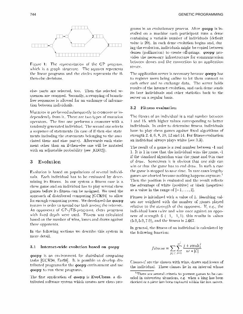
Figure 1: The representation of the GP program,

which is a graph structure. The squares represents

the linear programs and the circles represents the if-

then-else decisions.

else- parts are selected, too. Then the selected se-

quences are swapped. Secondly, a swapping of branch-

free sequences is allowed for an exchange of informa-

tion between individuals.

Mutation is performed subsequently to crossover or in-

dependently from it. There are two types of mutation

operators. The �rst one performs a crossover with a

randomly generated individual. The second one selects

a sequence of statements (in case of if-then-else state-

ments including the statements belonging to the asso-

ciated then- and else- parts). Afterwards each state-

ment other than an if-then-else one will be mutated

with an adjustable probability (see [KB02]).

3 Evolution

Evolution is based on populations of several individ-

uals. Each individual has to be evaluated by deter-

mining its �tness. In our system a �tness case is a

chess game and an individual has to play several chess

games before its �tness can be assigned. We used the

approach of distributed computing [GCK94] to allow

for enough computing power. We developed the qoopy

system in order to spread our task among the internet.

As opponents of GP-/ES-programs, chess programs

with �xed depth were used. Fitness was calculated

based on the number of wins, losses and draws against

these opponents.

In the following sections we describe this system in

more detail.

3.1 Internet-wide evolution based on qoopy

qoopy is an environment for distributed computing

tasks [GCK94, Far98]. It is possible to develop dis-

tributed programs for the qoopy environment and use

qoopy to run these programs.

The �rst application of qoopy is EvoChess, a dis-

tributed software system which creates new chess pro-

grams in an evolutionary process. After qoopy is in-

stalled on a machine each participant runs a deme

containing a variable number of individuals (default

value is 20). In each deme evolution begins and, dur-

ing the evolution, individuals might be copied between

demes (pollination) to create o�springs. qoopy pro-

vides the necessary infrastructure for communication

between demes and the connection to an application

server.

The application server is necessary because qoopy has

to register users being online to let them connect to

each other and to exchange data. The server holds

results of the internet evolution, and each deme sends

its best individuals and other statistics back to the

server on a regular basis.

3.2 Fitness evaluation

The �tness of an individual is a real number between

1 and 15, with higher values corresponding to better

individuals. In order to determine �tness, individuals

have to play chess games against �xed algorithms of

strength 2, 4, 6, 8, 10, 12 and 14. For �tness evaluation

an individual always plays white (see 3.3).

The result of a game is a real number between -1 and

1. It is 1 in case that the individual wins the game, -1

if the standard algorithm wins the game and 0 in case

of draw. Sometimes it is obvious that one side can

win or that the game has to end draw. In such a case

the game is stopped to save time. In rare cases lengthy

games are aborted because nothing happens anymore.1

Then the position is evaluated and the result re ects

the advantage of white (positive) or black (negative)

as a value in the range of [�1; : : : ; 1].

Fitness is initialized with a value of 1. Resulting val-

ues are weighted with the number of games played

relative to the strength of the opponent. If, e.g., the

individual loses twice and wins once against an oppo-

nent of strength 6 (�1;�1; 1), this results in values

(5:0; 5:0; 7:0), and the �tness is 5:667.

In general, the �tness of an individual is calculated by

the following function:

fitness =X

j2C

njX

i=1

j + resultj

i

nj � jCj

Classes C are the classes with wins, draws and losses of

the individual. These classes lie in an interval whose

1There are several criteria to prevent games to be can-

celed in interesting situations, e.g. when a king has been

checked or a piece has been captured within the last moves.


bounds are de�ned by the following rules: If an in-

dividual wins all its games up to class i, these results

are ignored and if an individual loses all its games from

class i to the highest class, these results are ignored.

For example if an individual i wins all games of classes

2, 4, and 8, and has wins, draws and losses in the

classes 6 and 10, and loses all games in the classes 12

and 14, Ci holds the classes 6, 8 and 10. The �rst rule

de�nes the lower bound of the interval (4), and the

second rule de�nes the upper bound of the interval

(12). The �rst rule does not hold for class 8 because

in class 6 the individual has had a draw or loss.

In general, the �tness of an individual is calculated in

four phases. Thus weak individuals can be dropped

from �tness evaluation in the �rst or second phase.

Fitness evaluation in phase three and four is very CPU

time expensive and we try to reduce the computation

time by removing inviable programs.

In phase one the individual plays two games against 2.

If the individual is very weak it can be identi�ed by the

�tness function and replaced immediately. In the sec-

ond phase the individual plays against 4, 6, 8 and 10.

If the �tness is at least 4.5 at the end of phase two, the

evaluation is continued in phase three. In phase three

the individual plays 1-2 games against 2, 4, 6, 8 and 10.

Successful individuals might skip games against 2 and

4. These are individuals which win each game up to

strength 6 and receive good results in games against 8

and 10. In phase four games are performed against 12

and 14. Only the best individuals play in this phase,

however. Games against the standard algorithm of

class 12 and 14 are very expensive.

To play more than twice against class 12 (or 14) it is

required to win in one of the two games before. Every

draw results in 1 point, every loss in 2 points. If the

individual has more than 6 (5) points it does not play

any more against class 12 (14). If the individual is

good enough it will play 4 times against 12 and then

3 times against 14.

3.3 Opponents of the individuals (black

players)

The opponents of individuals are chess programs which

can fully traverse the search tree up to a �xed depth.

We use these players to calculate the �tness of an indi-

vidual, by playing against �xed programs of di�erent

search depth. Fixed programs can play to a depth of

1, 2, 3, 4, 5, 6 and 7. Each of these programs de�nes

a corresponding �tness class of 2, 4, 6, 8, 10, 12 and

14. The value for a �tness class is the search depth

multiplied with 2, so that an individual which defeats

Figure 2: Average number of nodes used in the search

tree for di�erent �xed search depths. For search depth

6 the plot shows a large di�erence between a random

move ordering and an evolved move ordering module.

Even the f-negascout search algorithm requires more

resources than an evolved individual. The data are av-

erage values of more than 1000 moves (from reference

games).

an individual of class 4 but loses against an individual

of class 6 can be inserted into class 5.

The GP/ES individuals use a position evaluation of

the same structure and the same criteria - but their

weights are determined by the individual's genotype.

To reduce the number of nodes of the game tree an

f-negascout algorithm [Rei89] combined with iterative

deepening is performed for the black players. The f-

negascout algorithm is an improved variant of alpha-

beta, which is the most wide-spread tree search algo-

rithm. Iterative deepening performs a search to depth

d� 1 before searching to depth d (recursively). In ad-

dition, so-called killer moves are stored and tried �rst

whenever possible. Killer moves are moves which re-

sult in the cut of a subtree. This means that much of

the game tree can be discarded without loss of infor-

mation!

4 Results

In this section we describe the current results of an

ongoing evolution on the internet.

First we look at the evolved individuals and their eÆ-

ciency in search. The question is: How many resources

are needed by the evolved move ordering modules in

case of a �xed-depth search in comparison to other

move ordering strategies. Figure 2 shows the number


Figure 3: Box plot diagram of average number of used

nodes during a game with one of an evolved individual

combined with a simple �xed-depth alpha-beta algo-

rithm, average taken over more than 5000 moves from

50 reference games. The bar in the gray boxes is the

median of the data. A box represents 50 % of the

data, this means that 25 % of the data lies under and

over a box. The smallest and biggest usual values are

connected with a dashed line. The circles represents

outliers of the data.

of nodes examined in the search tree of an alpha-beta-

algorithm with a random move ordering, an evolved

individual and the f-negascout algorithm (the oppo-

nent of an individual (the black player) is always an

f-negascout algorithm). The �gure shows that a ran-

dom move ordering algorithm calculates seven million

nodes with a search tree of depth 6. The f-negascout

algorithm needs one million nodes. An evolved in-

dividual only needs 250,000 nodes. So evolution has

managed to create individuals which perform a very

eÆcient search through the tree.

Figures 3 and 4 show a box plot diagram investigat-

ing the number of search nodes visited by an evolved

and a random move ordering module combined with a

simple �xed-depth alpha-beta algorithm. The evolved

individual clearly outperforms the random one. Be-

sides, the �gures show that most nodes during a game

are used between ply 10 and 60.

The other aspect of the evolved chess programs is the

quality of the selected moves. Currently evolution suc-

ceeded to evolve a chess playing program, with a �t-

ness of 10.48. This means that the evolved program is

better than the opponent program of �tness class 10.

The �tness value was measured by a post-evaluation of

best programs: An individual plays 20 games against

class 8, 10 and 12, so that the �tness value is the re-

Figure 4: Box plot diagram of average number of used

nodes during a game with a random individual (see

also �gure 3).

sult of 60 games. Note that the individual achieves

this result by expanding on average 58,410 nodes per

move in the search tree. A simple alpha-beta chess pro-

gram needs 897,070 nodes per move for search depth

of 5, which corresponds to class 10. The f-negascout

algorithm which is an improved variant of alpha-beta,

needs 120,000 nodes per move for this search depth.

In other words evolution has improved the search al-

gorithm, so that it wins by only using 50% of the re-

sources of a f-negascout algorithm which, in turn, out-

performs an alpha-beta-algorithm. Evolved individu-

als win against a simple alpha-beta-algorithm by using

only 6% of the resources.

5 Summary and Outlook

We have shown, that it is possible to evolve chess play-

ing individuals superior to given algorithms. At this

time evolution is still going on and results are still im-

proving.

Next we shall develop this approach by using other

search algorithms as the internal structure, and by ex-

changing the di�erent modules. A further feature will

be that individuals will play against each other.

The ultimate goal of our approach is to beat computer

programs like Deep Blue, which to this day use brute-

force methods to play chess.

ACKNOWLEDGMENT

The authors gratefully acknowledge the enthusiastic

support of a large group of EvoChess users. A


list of participants is available at http://qoopy.cs.uni-

dortmund.de/qoopy e.php?page=statistik e . All of

them have helped to produce these results and to im-

prove both EvoChess and the qoopy system con-

siderably. Support has been provided by the DFG

(Deutsche Forschungsgemeinschaft), under grant Ba

1042/5-2.

SUPPLEMENTARY MATERIAL

More information on the qoopy system, the EvoChess

application, and experimental data are available from:

http://www.qoopy.net.

References

[Bea99] D.F. Beal. The Nature of Minimax

Search. PhD thesis, University of Maas-

tricht, 1999. Diss.Nr.99-3.

[BK77] J. Birmingham and P. Kent. Tree-

Searching and Tree-Pruning Techniques.

In M.R.B. Clarke, editor, Advances in

Computer Chess 1, pages 89{97. Edin-

burgh University Press, 1977.

[BKA+00] J. Busch, W. Kantschik, H. Aburaya,

K. Albrecht, R. Gross, P. Gundlach,

M. Kleefeld, A. Skusa, M. Villwock,

T. Vogd, and W. Banzhaf. Evolu-

tion von GP-Agenten mit Schachwissen

sowie deren Integration in ein Comput-

erschachsystem. SYS Report SYS-01/00,

ISSN 0941-4568, Systems Analysis Re-

search Group, Univ. Dortmund, Infor-

matik, 10 2000.

[BNKF98] W. Banzhaf, P. Nordin, R. E. Keller,

and F. D. Francone. Genetic Program-

ming { An Introduction On the Automatic

Evolution of Computer Programs and its

Applications. Morgan Kaufmann, San

Francisco und dpunkt verlag, Heidelberg,

1998.

[BR58] A. Bernstein and M. de V. Roberts. Com-

puter v Chess-Player. Scienti�c Ameri-

can, 198:96{105, 1958.

[Far98] J. Farley. Java Distributed Computing.

O'Reilly, 1998.

[GCK94] J. Dollimore G.F. Coulouris and T. Kind-

berg. Distributed Systems, Concepts and

Design. Addison-Wesley, 2 edition, 1994.

[IHU95] H. Iida, K. Handa, and J. Uiterwijk. Tu-

toring Strategies in Game-Tree Search.

ICCA Journal, 18(4):191{205, December

1995.

[KB01] W. Kantschik and W. Banzhaf. Linear-

tree GP and its comparison with other GP

structures. In J. F. Miller, M. Tomassini,

P. Luca Lanzi, C. Ryan, A. G. B. Tet-

tamanzi, and W. B. Langdon, editors,

Genetic Programming, Proceedings of Eu-

roGP'2001, volume 2038 of LNCS, pages

302{312, Lake Como, Italy, 18-20 April

2001. Springer-Verlag.

[KB02] W. Kantschik and W. Banzhaf. Linear-

graph gp - a new gp structure. In J. F.

Miller, M. Tomassini, P. Luca Lanzi,

C. Ryan, A. G. B. Tettamanzi, and

W. B. Langdon, editors, Genetic Pro-

gramming, Proceedings of EuroGP'2002,

LNCS. Springer-Verlag, 2002.

[Kor97] R.E. Korf. Does Deep Blue Use Arti�cial

Intelligence? ICCA Journal, 20(4):243{

245, December 1997.

[NB95] Peter Nordin and Wolfgang Banzhaf.

Evolving turing-complete programs for a

register machine with self-modifying code.

In L. Eshelman, editor, Genetic Algo-

rithms: Proceedings of the Sixth Interna-

tional Conference (ICGA95), pages 318{

325, Pittsburgh, PA, USA, 15-19 1995.

Morgan Kaufmann.

[Nor94] J. P. Nordin. A Compiling Genetic Pro-

gramming System that Directly Manipu-

lates the Machine code, pages 311{331.

MIT Press, Cambridge, 1994.

[PSPDB96] A. Plaat, J. Schae�er, W. Pijls, and

A. De Bruin. Best-�rst �xed-depth min-

imax algorithms. Arti�cial Intelligence,

87:255{293, 1996.

[Rei89] A. Reinfeld. An improvement of the scout

tree search algorithm. ICCA Journal,

6(4):4{14, June 1989.

[Sch89] J. Schae�er. The History Heuristic

and Alpha-Beta Search Enhancements in

Practice. IEEE Transactions on Pat-

tern Analysis and Machine Intelligence,

11(11):1203{1212, 1989.

[Sch96] H-P. Schwefel. Evolution and Optimum

Seeking. John Wiley & Sons, Inc., 1996.


Breeding Algebraic Structures – An Evolutionary Approach toInductive Equational Logic Programming

Lutz HamelDepartment of Computer Science and Statistics

University of Rhode Island, Kingston, Rhode Island 02881, USAemail: [email protected]

Abstract

Concept learning is the induction of a de-scription from a set of examples. Inductivelogic programming can be considered a spe-cial case of the general notion of conceptlearning specifically referring to the inductionof first-order theories. Both concept learn-ing and inductive logic programming can beseen as a search over all possible sentencesin some representation language for sentencesthat correctly explain the examples and alsogeneralize to other sentences that are part ofthat concept. In this paper we explore in-ductive logic programming with equationallogic as the representation language and ge-netic programming as the underlying searchparadigm. Equational logic is the logic ofsubstituting equals for equals with algebrasas models and term rewriting as operationalsemantics.

1 INTRODUCTION

The aim of concept learning is to induce a descriptionof a concept from a set of examples. Typically the setof examples are ground sentences in a particular rep-resentation language. Concept learning can be seen asa search over all possible sentences in the representa-tion language for sentences that correctly explain theexamples and also generalize to other sentences thatare part of that concept [11, 16]. Inductive logic pro-gramming (ILP) can be considered a special case of thegeneral notion of concept learning specifically referringto the induction of first-order theories as descriptionsof concepts [17].

Specialized search mechanisms for specific representa-tion languages have been devised over the years. For

example, in the propositional setting we have Quin-lan’s entropy based decision tree algorithm ID3 [21].In the first-order logic setting we have Muggleton’sinductive logic programming system Progol whose un-derlying search paradigm is based on inverting logicalentailment [19].

Since concept learning and inductive logic program-ming imply complex searches, it is natural to askwhether evolutionary algorithms are applicable in thisarea. Briefly, evolutionary algorithms are a class of al-gorithms that traverse complex search spaces by mim-icking natural selection. The algorithms maintain alarge population of individuals with different charac-teristics where each individual represents a point in thesearch space. By exerting selective pressures on thispopulation, fitter individuals representing better solu-tion points according to the search criteria will emergefrom the population. These fitter individuals in turnare allowed to reproduce in a preferential manner insubsequent generations increasing the overall fitness ofthe population. At the end of the run the fittest indi-viduals in the final population represent the final solu-tion points in a complex search space [9, 14]. To dateevolutionary algorithms, particularly genetic program-ming systems, have successfully been applied to con-cept learning and inductive logic programming tasks ina variety of formalisms. For example, they have beensuccessfully applied in the propositional case [13], inthe first-order logic setting [24, 10], as well as in thehigher-order functional logic programming setting [11].

In this paper we examine an evolutionary approach toconcept learning based on another formalism – many-sorted first-order equational logic. Equational logic isthe logic of substituting equals with equals. Here theexamples are ground equations and the induced con-cept descriptions are first-order equational theories.We have implemented a prototype by incorporating aspecialized genetic programming engine into the equa-tional logic programming system and algebraic speci-


fication language OBJ3 [5, 6]. Informally, the systemoperates by maintaining a population of candidate the-ories that are evaluated against the examples usingOBJ3’s deductive machinery. The fittest theories areallowed to reproduce in accordance to standard ge-netic programming practices. Because of the fact thatwe are inducing first-order equational theories we tendto refer to this approach as inductive equational logicprogramming.

This search based view of inductive logic programmingis a very operational view. It is possible to formulatea semantics to inductive logic programming that is in-dependent of any particular search strategy. We willdiscuss this normal semantics to ILP in more detailbelow. Equational theories have a very strong notionof sorts and operators; i.e., they have a very strongnotion of signatures. We recast the first-order logicnormal semantics for ILP into an algebraic light thatdeals with the strong notion of signature effectively.This algebraic formulation of the normal semantics forILP forms the basis of our system implementation withthe genetic programming strategy as the operationalsemantics.

The system most closely related to ours is the FLIPsystem [2, 7]. It also concerns itself with the inductionof first-order equational theories from ground equa-tions. However, the FLIP system uses inverse narrow-ing as a search strategy instead of the evolutionary ap-proach as advocated here. On a technical equationallogic level the FLIP system deals with signatures onlyimplicitly, which means that by design it is limited tosingle-sorted equational logic.

The rest of this paper is organized as follows. Sec-tion 2 provides a brief introduction to many-sortedequational logic, algebra and term rewriting. In Sec-tion 3 we examine the normal semantics for inductivelogic programming. We develop an algebraic seman-tics for our setting in Section 4. Section 5 sketchesour system implementation. In Section 6 we take acritical look at results obtained with the preliminaryimplementation so far. We end with the conclusionsin Section 7.

2 EQUATIONAL LOGIC

Equational logic is the logic of substituting equals forequals with algebras as models and term rewriting asthe operational semantics [15, 23, 1]. The followingformalizes these notions.

An equational signature defines a set of sort symbolsand a set of operator or function symbols.

Definition 1 An equational signature is a pair(S,Σ), where S is a set of sorts and Σ is an (S∗×S)-sorted set of operation names. The operator σ ∈ Σw,sis said to have arity w ∈ S∗ and sort s ∈ S. Usuallywe abbreviate (S,Σ) to Σ. 1

We define Σ-algebras as models for these signatures asfollows:

Definition 2 Given a many sorted signature Σ, a Σ-algebra A consists of the following:

• an S-sorted set, usually denoted A, called the car-rier of the algebra,

• a constant Aσ ∈ As for each s ∈ S and σ ∈ Σ[],s,

• an operation Aσ : Aw → As, for each non-empty list w = s1 . . . sn ∈ S∗, and each s ∈ Sand σ ∈ Σw,s, where Aw = As1 × . . .×Asn.

Mappings between signatures map sorts to sorts andoperator symbols to operator symbols.

Definition 3 An equational signature morphismis a pair of mappings φ = (f, g) : (S,Σ)→ (S′,Σ′), wewrite φ : Σ→ Σ′.

A theory is an equational signature with a collectionof equations.

Definition 4 A Σ-theory is a pair (Σ, E) whereΣ is an equational signature and E is a set of Σ-equations. Each equation in E has the form (∀X)l =r, where X is a set of variables distinct from the equa-tional signature Σ and l, r ∈ TΣ(X) are terms over theset Σ and X. If X = ∅, that is, l and r contain novariables, then we say the equation is ground. Whenthere is no confusion Σ-theories are referred to as the-ories and are denoted by their collection of equations,in this case E.

The above can easily be extended to conditionalequations2. However, without loss of generality wecontinue the discussion here based on unconditionalequations only. Also, our current prototype solely

1Notation: Let S be a set, then S∗ denotes the setof all finite lists of elements from S, including the emptylist denoted by []. Given an operation f from S into aset B, f : S → B, the operation f∗ denotes the exten-sion of f from a single input value to a list of input val-ues, f∗ : S∗ → B, and is defined as follows: f∗(sw) =f(s)f∗(w) and f∗([]) = [], where s ∈ S and w ∈ S∗.

2Consider the conditional equation, (∀X)l = r if c,which is interpreted as meaning the equality holds if thecondition c is true.


considers the evolution of theories with unconditionalequations.

The models of a theory are the Σ-algebras that sat-isfy the equations. Intuitively, an algebra satisfies anequation if and only if the left and right sides of theequation are equal under all assignments of the vari-ables. More formally:

Definition 5 A Σ-algebra A satisfies a Σ-equation(∀X)l = r iff θ(l) = θ(r) for all assignmentsθ : TΣ(X) → A. We write A |= e to indicate thatA satisfies the equation e.

We define satisfaction for theories as follows:

Definition 6 Given a theory T = (Σ, E), a Σ-algebraA is a T -model if A satisfies each equation e ∈ E. Wewrite A |= T or A |= E.

In general there are many algebras that satisfy a par-ticular theory. We also say that the class of algebrasthat satisfy a particular equational theory representthe denotational semantics of that theory.

Semantic entailment of an equation from a theory isdefined as follows.

Definition 7 An equation e is semantically en-tailed by a theory (Σ, E), write E |= e, iff A |= Eimplies A |= e for all Σ-algebras A.

Mappings between theories are defined as theory mor-phisms.

Definition 8 Given two theories T = (Σ, E) andT ′ = (Σ′, E′), then a theory morphism φ : T → T ′

is a signature morphism φ : Σ → Σ′ such that E′ |=φ(e), for all e ∈ E.

In other words, the signature morphism φ is a theorymorphism if the translated equations of the source the-ory T are semantically entailed by the target theoryT ′.

Goguen and Burstall have shown within the frameworkof institutions [1] that the following holds for manysorted algebra3:

Theorem 9 Given the theories T = (Σ, E) and T ′ =(Σ′, E′), the theory morphism φ : T → T ′, and the T ′-algebra A′, then A′ |=Σ′ φ(e) ⇒ φA′ |=Σ e, for alle ∈ E.

3Actually, Goguen and Burstall have shown the muchmore powerful result that the implication holds as an equiv-alence relation. However, for our purposes here we onlyneed the implication.

In other words, if we can show that a given model ofthe target theory satisfies the translated equations ofthe source theory, it follows that the reduct of thismodel, φA′, also satisfies the source theory, thus, themodels behave as expected.

Our approach to equational logic so far has been purelymodel theoretic. A proof theory for many-sorted equa-tional logic is defined by the following rules of deduc-tion. Given a signature Σ and a set of Σ-equations,the following are the rules for deriving new equations[15] (here t, u, and v denote terms over the signatureΣ and an appropriate variable set):

1. Reflexivity. Each equation (∀X)t = t is derivable.

2. Symmetry. If (∀X)t = t′ is derivable, then so is(∀X)t′ = t.

3. Transitivity. If the equations (∀X)t = t′,(∀X)t′ = t′′ are derivable, then so is (∀X)t = t′′.

4. Substitutivity. If (∀X)t1 = t2 of sort s is deriv-able, if x ∈ X is of sort s′, and if (∀Y )u1 = u2of sort s′ is derivable, then so is (∀Z)v1 = v2,where Z = (X − {x}) ∪ Y , vj = tj(x ← uj) forj = 1, 2, and ‘tj(x ← uj)’ denotes the result ofsubstituting uj for x in tj.

5. Abstraction. If (∀X)t = t′ is derivable, if y is avariable of sort s and y is not in X, then (∀X ∪{y})t = t′ is also derivable.

6. Concretion. Let us say that a sort s is void in asignature Σ iff TΣ,s = ∅. Now, if (∀X)t = t′ isderivable, if x ∈ Xs does not appear in either t ort′, and if s is non-void, then (∀X − {x})t = t′ isalso derivable.

Given a theory (Σ, E), we say that an equation(∀X)t = t′ is deducible from E if there is a deduc-tion from E using rules 1-6 whose last equation is(∀X)t = t′ [23]. We write: E ` (∀X)t = t′.

The model theoretic and the proof theoretic ap-proaches to equational logic are related by the notionof soundness and completeness.

Theorem 10 (Soundness and Completeness ofEquational Logic) Given an equational theory(Σ, E), an arbitrary equation (∀X)t = t′ is semanti-cally entailed iff (∀X)t = t′ is deducible from E. For-mally, E |= (∀X)t = t′ iff E ` (∀X)t = t′, wheret, t′ ∈ TΣ(X).

This theorem is very convenient, since it lets us useequational deduction to check the theory morphism


conditions above which plays an important part in oursystem implementation.

Term rewriting [12, 15] can be considered an efficientimplementation of unidirectional equational deductionby viewing equations as rewrite rules from left to right.Given a Σ-equation (∀X)t = t′, consider: a term t0 canbe rewritten into a term t1 provided that t0 contains asubterm that is a substitution instance of the left sidet of the equation. Then t1 is the result of replacing thesubstitution instance of t with the appropriate substi-tution instance of t′ in t0. Given this, every term canbe rewritten to a unique canonical form under mildconditions on the set E of Σ-equations, such as everyvariable of a right side of an equation must also appearin the left side. This forms the basis of the operationalsemantics of the OBJ specification language [5, 6].

3 INDUCTIVE LOGICPROGRAMMING

Traditionally, inductive logic programming has con-cerned itself with the induction of first-order logictheories from facts and background knowledge. Thenormal semantics for ILP is usually stated as follows[3, 20],

Definition 11 Given a set B of horn clause defini-tions (background theory), a set P of ground facts tobe entailed (positive examples), a set N of ground factsnot to be entailed (negative examples), and a hypothe-sis language L, then a construct H ∈ L is an hypoth-esis if

B ∪H |= p, for every p ∈ P (Completeness),B ∪H 6|= n, for every n ∈ N (Consistency).

Here, L is the set of all well-formed logical formu-lae over a fixed vocabulary. Completeness states thatthe conjunction of the background and the hypothesisentail the positive facts. Consistency states that thebackground and the hypothesis do not entail the neg-ative facts or counter examples. Logical entailment isderived by interpreting the clauses in the appropriateHerbrand models [22].

Please note that this semantic definition does not sayanything about the quality of a particular hypothe-sis. In fact, it is interesting to note that this seman-tic definition admits a number of trivial solutions; forinstance, let H = P . Also consider the case whereB |= p for every p ∈ P . Typically, the weighing ofone hypothesis over another is left to the operationalor search semantics of an ILP system. In practicalILP systems trivial solutions like the ones above are

typically immediately dismissed by the system on itssearch for an “optimal” hypothesis, since these trivialsolutions tend not to pass a set of performance criteriawhen compared to other more general hypotheses.

4 AN ALGEBRAIC SEMANTICS

The above semantics for ILP treats signatures implic-itly. However, type information and signatures playa central role in many-sorted equational logic. There-fore, we recast the above semantics in an algebraicsetting based on signatures, equational theories, andtheory morphisms. We start by defining what we meanby facts.

Definition 12 A theory (Σ, E) is called Σ-facts ifeach e ∈ E is a ground equation.

This allows us to define our notion of induced theory.

Definition 13 Given a background theory B =(ΣB , EB), positive facts P = (ΣP , EP ), and nega-tive facts N = (ΣN , EN ), then an induced theoryH = (ΣH , EH), is a theory with a pair of mappingsφB and φP

H

B

φB

>>~~~~~~~~P

φP

``@@@@@@@

such that

• φB : B → H is a theory morphism,

• φP : P → H is a theory morphism,

• and H 6|= φN (e), for all e ∈ EN , and signaturemorphism φN : ΣN → ΣH .

Our induced theory is not unlike the hypothesis in thenormal semantics. In fact, by making φB an inclu-sion morphism we have the algebraic equivalent for-mulation of the normal semantics for ILP. We like theadded generality our semantics supports and will ex-plore this in future implementations. Currently, theprototype interprets φB as the inclusion morphism.

Taking a closer look at φB , from the definition we haveφB : B → H is a theory morphism if H |= φB(e), foreach e ∈ EB . This is equivalent of saying that in orderfor this mapping to be valid the induced theory mustsemantically entail the given background knowledge.Of course this holds trivially if φB is the inclusion mor-phism.

A closer look at the theory morphism φP that maps thepositive facts into the induced theory reveals a similar


relationship. Again from the definition, φP : P → His a theory morphism if H |= φP (e), for each e ∈ EP .This can be considered the algebraic formulation ofthe completeness criteria of the normal ILP seman-tics. Please note, by replacing the semantic entailmentwith proof theoretic deduction which follows from thesoundness and completeness of equational logic we ob-tain a computable relation. This is precisely what weuse in our system implementation below.

The last part of the definition above is the algebraicformulation of the consistency statement: negativefacts should not be entailed by the induced theory.Similar to the normal semantics our algebraic seman-tics says nothing about the quality of the induced the-ory. This is left to the search semantics of the system;in our case this is left to the genetic programming en-gine.

So far we have treated models that satisfy H implicitly.It is interesting to take a look at the models per se.

Proposition 14 Given an induced theory H, with thebackground theory B, the positive facts P , and the neg-ative facts N , then each model m that satisfies theinduced theory H and is consistent with the negativefacts N also satisfies the background theory B and thepositive facts P .

Proof: From the previous section we know that forevery theory morphism φ : T → T ′ and a model m′ |=T ′ there is a reduct φm′ such that φm′ |= T . Letus assume that there exists a model m that satisfiesthe induced theory H and is consistent with N , i.e.,m |= H and m 6|= N . We then have two reducts alongthe theory morphisms φB : B → H and φP : P → H,namely φBm and φPm, respectively, where φBm |= Band φPm |= P . Thus, consistent models that satisfythe induced theory H have reducts along the theorymorphisms and behave as expected. 2

5 SYSTEM IMPLEMENTATION

We have implemented our prototype system within theOBJ3 algebraic specification system [5, 6]. OBJ3 im-plements many-sorted equational logic4 with algebrasas its denotational semantics and many-sorted termrewriting as its operational semantics.

The following specification of a stack of elements canbe considered a prototypical OBJ3 specification.

4Actually, OBJ3 implements order-sorted equationallogic, which means that the sorts are related to each otherthrough a type lattice. In our current implementation wedo not support this type ordering.

obj STACK is sorts Stack Element .op empty : -> Stack .op push : Stack Element -> Stack .op top : Stack -> Elementop pop : Stack -> Stack .var X : Element . var S : Stack .eq top(push(S,X)) = X .eq pop(push(S,X)) = S .

endo

The first line of the specification names the theory andalso defines two sorts; namely, Stack and Element.The following four lines define the operations on thestack. We then define the variables we need in theequations on the following two lines.

The current prototype incorporates a genetic program-ming engine based on Koza’s canonical LISP imple-mentation [14] into the OBJ3 system. The engineperforms the following steps given a (possibly empty)background theory and the facts:

1. Compute initial (random) population of candi-date theories;

2. Evaluate each candidate theory’s fitness using theOBJ3 rewrite engine;

3. Perform candidate theory reproduction accordingto the genetic programming paradigm;

4. Compute new population of candidate theories;

5. Goto step 2 or stop if target criteria have beenmet.

This series of steps does not significantly differ fromthe standard genetic programming paradigm. Thefittest individual of the final population is consideredto be the induced theory satisfying the given facts.

A couple of things are noteworthy. The signatures ofthe candidate theories are computed using the signa-ture morphism constructions underlying the algebraicsemantics outlined above. Both, for the backgroundtheory as well as for the positive facts we let the sig-nature morphisms be inclusions. In order to completethe candidate theories the system adds equations tothe computed signatures according the to the geneticprogramming paradigm.

For the negative facts we take advantage of OBJ3’sbuiltin boolean operator =/=. This operator allowsus to recast negative facts as inequality relations thatneed to hold in the candidate theories. In effect, theseinequalities become positive facts and we treat themas such by adding them to the positive facts theory.Consequently we set the negative fact theory to theempty theory. This technique facilitates the codingfor the genetic programming engine, since the notion


of positive facts aligns very nicely with the notion offitness cases in the genetic programming paradigm. Anexample of this technique can be seen in the resultssection.

The system uses the OBJ3 rewrite engine to evalu-ate candidate theories against the positive facts. Theproof obligation arises from the theory morphism con-dition for the positive facts. Given a fact equationand a candidate theory, the theory morphism condi-tion is tested by rewriting the left and right sides ofthe fact equation to their unique canonical forms usingthe equations of the candidate theory as rewrite rules.If the unique canonical forms of the left and right sidesare equal then the fact equation is said to hold.

Since the equations in the candidate theories are gener-ated at random, there is no guarantee that the theoriesdo not contain circularities throwing the rewriting en-gine into an infinite rewriting loop when evaluating thefacts. To guard against this situation we allow the userto set a parameter that limits the number of rewritesthe engine is allowed to do per fact evaluation. Thispragmatic approach proved very effective. The alter-native would have been an in-depth analysis of theequations in each candidate theory adding significantoverhead to the execution time of the evolutionary al-gorithm. In some sense this is analogous to guardingagainst division by zero when evaluating arithmeticexpressions within the canonical genetic programmingparadigm.

The fitness function used by the system to evaluateeach candidate theory is

fitness(T ) = (facts(T ))2 +1

length(T ),

where T denotes a candidate theory, facts(T ) is thenumber of facts or fitness cases entailed by the can-didate theory, and length(T ) is the number of equa-tions in the candidate theory. The fitness function isdesigned to primarily exert evolutionary pressure to-wards finding candidate theories that match all thefacts (the first term of the function). In addition, inthe tradition of Occam’s Razor [8] the function also ex-erts pressure towards finding the shortest theory thatsupports all the facts (second term). The system at-tempts to maximize this function in each generationof candidate theories.

The genetic programming engine itself is implementedas a strongly typed genetic programming system [18, 4]in the sense that it knows about the syntactic structureof theories and equations and does not have to redis-cover these notions with every run. The only geneticoperators we have implemented so far are fitness pro-portionate reproduction and a type sensitive crossover

operator. We found that mutation proved too disrup-tive probably due to our incomplete type system im-plementation, as the current prototype does not prop-erly support user declared equational logic types. Thisdid not prevent us from performing some interestingexperiments, however. We are currently working onthe next generation system that supports user definedtypes fully.

6 EXPERIMENTS AND RESULTS

To study the system we performed three experimentswith encouraging results. These experiments were in-spired by case studies on the FLIP home page [2].

6.1 INFERRING STACK PROPERTIESFROM EXAMPLES

In the first example we were looking for the generalconcept of the stack operator top given a set of facts.The facts are as follows:

obj STACK-FACT is sort Sort .ops a b u v s: -> Sort .op top : Sort -> Sort .op push : Sort Sort -> Sort .eq top(push(v,a)) = a .eq top(push(push(v,a),b)) = b .eq top(push(push(v,b),a)) = a .eq top(push(push(v,u),s)) = s .

endo

Each ground equation in the fact theory gives a spe-cific application instance of the operator top. We ex-pect the equational inductive logic system to discovera theory that generalizes the description the operatorbeyond the seen instances. After 28 generations with200 individuals the system discovered the following in-duced theory:

obj STACK is sort Sort .ops a b u v s: -> Sort .op top : Sort -> Sort .op push : Sort Sort -> Sort .vars X1 X2 X3 X4 X5 : Sort .eq top(push(X4,X2)) = X2 .

endo

This theory correctly characterizes all the groundequations in the fact theory by stating that the topof a stack is the last element pushed. The followingparameters were used during this run:

Maximum number of Generations: 60Size of Population: 200Maximum equations for theories: 4Maximum Rewrites: 20Maximum depth of new individuals: 5Maximum depth of new subtrees for mutants: 5Maximum depth of individuals after crossover: 10Fitness-proportionate reproduction fraction: 0.1Crossover at any point fraction: 0.8Crossover at function points fraction: 0.1Number of fitness cases: 4Selection method: fit-propGeneration method: rampedRandomizer seed: 1.0


The Maximum Rewrites parameter limits the numberof rewrites the OBJ3 rewriting engine is allowed toperform when evaluating a fact. Readers familiar withKoza’s implementation will notice that the above pa-rameter setting does not allow for mutation.

6.2 INFERRING A RECURSIVEFUNCTION DEFINITION

In the following example we want to infer the recur-sive definition of the function sum from a set of groundequations. The fact theory is given in Peano nota-tion where the naturals are represented as s(0) 7→ 1,s(s(0)) 7→ 2, etc. The fact theory is as follows:

obj SUM-FACT is sort Sort .op 0 : -> Sort .op s : Sort -> Sort .op sum : Sort Sort -> Sort .eq sum(0,0) = 0 .eq sum(s(0),s(0)) = s(s(0)) .eq sum(0,s(0)) = s(0) .eq sum(s(s(0)),0) = s(s(0)) .eq sum(s(0),0) = s(0) .eq sum(s(0),s(s(0)))= s(s(s(0))) .eq sum(s(s(0)),s(s(0)))= s(s(s(s(0)))) .eq sum(s(s(s(0))),s(0)) = s(s(s(s(0)))) .eq sum(s(s(s(0))),s(s(0))) = s(s(s(s(s(0))))) .eq (s(0) =/= 0) = true .eq (s(s(0)) =/= 0) = true .eq (s(s(s(0))) =/= 0) = true .eq (sum(s(0),0) =/= 0) = true .eq (sum(0,0) =/= s(0)) = true .eq (sum(s(0),s(0)) =/= s(0)) = true .eq (sum(s(0),0) =/= s(s(0))) = true .eq (sum(0,s(0)) =/= s(s(0))) = true .eq (sum(0,s(0)) =/= 0) = true

endo

The first half of the theory are positive facts andthe second half are negative facts coded as positivefacts taking advantage of OBJ3’s builtin boolean op-erator =/=. As hinted at before, we take advantageof this builtin capability to express everything as posi-tive facts rather than trying to prove that the negativefacts do not hold in the induced theory. Additionally,this is more inline with the notion of fitness cases inthe genetic programming engine.

After 10 generations with 200 individuals the systemconverged on the following theory as the induced the-ory:

obj SUM is sort Sort .op 0 : -> Sort .op s : Sort -> Sort .op sum : Sort Sort -> Sort .vars X0 X1 : Sort .eq sum(X1,0) = X1 .eq sum(X1,s(X0)) = s(sum(X1,X0)) .

endo

The first equation of this recursive definition of theoperator sum states that that adding 0 to a value leavesthe value unchanged. The second equation states thatadding a value to the successor of another value is thesame as the successor of the sum of the two values.

The parameters for the genetic programming engine inthis experiment were:

Maximum number of Generations: 20Size of Population: 200Maximum equations for theories: 8Maximum Rewrites: 25Maximum depth of new individuals: 5Maximum depth of new subtrees for mutants: 5Maximum depth of individuals after crossover: 10Fitness-proportionate reproduction fraction: 0.1Crossover at any point fraction: 0.8Crossover at function points fraction: 0.1Number of fitness cases: 18Selection method: fit-propGeneration method: rampedRandomizer seed: 1.0

6.3 INFERRING ANOTHER RECURSIVEFUNCTION DEFINITION

In this last example we would like to infer the conceptof even from a set of facts. Again we use the Peanonotation for naturals. The fact theory is given as fol-lows:

obj EVEN-FACT is sort Sort .op 0 : -> Sort .op s : Sort -> Sort .op even : Sort -> Bool .eq even(0) = true .eq even(s(s(0))) = true .eq even(s(s(s(s(0))))) = true .eq (s(0) =/= 0) = true .eq (s(s(0)) =/= 0)= true .eq (s(s(s(0))) =/= 0) = true .eq (s(s(s(s(0)))) =/= 0) = true .eq (even(s(0)) =/= true) = true .eq (even(s(s(s(0)))) =/= true) = true .

endo

Please note that as in the previous example we employthe convention of coding negative examples as inequal-ities that must hold in the induced theory.

Unfortunately, here the system did not converge ona sensible induced theory even after as many as fiftygenerations with 200 individuals. We had expectedsomething like the following:

obj EVEN is sort Sort .op 0 : -> Sort .op s : Sort -> Sort .op even : Sort -> Bool .var X0 : Sort .eq even(s(s(X0))) = even(X0) .eq even(0) = true .

endo

We suspect that the failure to converge is due to thefact that in this particular case it is paramount to dis-tinguish between the user defined type Sort and thebuiltin type Bool. Due to the incomplete implemen-tation of our type system the genetic programmingengine is allowed to produce too many “junk” terms,i.e., syntactically malformed terms, which prevents thesystem from converging. We suspect that the systemwill not have any problems with this specification oncewe implement our type system fully.


7 CONCLUSIONS

Starting with the general notion of concept learningwe developed an approach to inductive logic program-ming based on many-sorted equational logic with ge-netic programming as the underlying search paradigm.Many-sorted equational logic has a strong notion ofsignature and we accommodated this by developing analgebraic semantics for inductive equational logic pro-gramming using the the normal semantics for inductivelogic programming as a starting point. Based on theseunderpinnings we implemented a prototype inductiveequational logic programming system within the alge-braic specification language OBJ3. Results of initialexperiments looked encouraging and we expect that amore complete implementation of the type system inthe prototype will remedy the current short comings.

References

[1] R. Burstall and J. Goguen. Institutions: abstractmodel theory for specification and programming.Journal of the Association for Computing Machinery,39(1):95–146, 1992.

[2] C. Ferri-Ramırez, J. Hernandez-Orallo, and M.J.Ramırez-Quintana. The FLIP system homepage,2000. http://www.dsic.upv.es/ flip/.

[3] P. A. Flach. The logic of learning: a brief intro-duction to inductive logic programming. In Proceed-ings of the CompulogNet Area Meeting on Computa-tional Logic and Machine Learning, pages 1–17, 1998.http://citeseer.nj.nec.com/flach98logic.html.

[4] P. A. Flach, C. Giraud-Carrier, and J. W. Lloyd.Strongly typed inductive concept learning. In D. Page,editor, Proceedings of the 8th International Confer-ence on Inductive Logic Programming, volume 1446,pages 185–194. Springer-Verlag, 1998.

[5] J. Goguen. The OBJ homepage. http://www-cse.ucsd.edu/users/goguen/sys/obj.html.

[6] J. Goguen, T. Winkler, J. Meseguer, K. Futatsugi,and J. Jouannaud. Software Engineering with OBJ:algebraic specification in action, chapter IntroducingOBJ. Kluwer, 2000.

[7] J. Hernandez-Orallo and M. J. Ramırez-Quintana. Astrong complete schema for inductive functional logicprogramming. In S. Dzeroski and P. Flach, editors,Proceedings of the 9th International Workshop on In-ductive Logic Programming, volume 1634, pages 116–127. Springer-Verlag, 1999.

[8] F. Heylighen. Principia cybernetica, July 1997.http://pespmc1.vub.ac.be/OCCAMRAZ.html.

[9] J. H. Holland. Adaptation in Natural and ArtificialSystems. University of Michigan Press, Ann Arbor,1975.

[10] R. Ichise. Inductive logic programming and geneticprogramming. In H. Prade, editor, European Confer-ence on Artificial Intelligence, 1998.

[11] C. J. Kennedy and C. Giraud-Carrier. An evolu-tionary approach to concept learning with structureddata. In Proceedings of the fourth International Con-ference on Artificial Neural Networks and Genetic Al-gorithms, pages 1–6. Springer Verlag, 1999.

[12] J. W. Klop. Term rewriting systems. In S. Abramsky,D. Gabbay, and T. Maibaum, editors, Handbook ofLogic in Computer Science, volume 2, pages 1–116.Oxford University Press, 1992.

[13] J. R. Koza. Concept formation and decision tree in-duction using the genetic programming paradigm. InH.-P. Schwefel and R. Manner, editors, Parallel Prob-lem Solving from Nature - Proceedings of 1st Work-shop, PPSN 1, volume 496, pages 124–128, Dortmund,Germany, 1-3 1991. Springer-Verlag.

[14] J. R. Koza. Genetic Programming: On the Program-ming of Computers by Natural Selection. MIT Press,Cambridge, MA, 1992.

[15] J. Meseguer and J. Goguen. Initiality, induction andcomputability. In M. Nivat and J. Reynolds, editors,Algebraic Methods in Semantics, pages 459–541. Cam-bridge, 1985.

[16] T. M. Mitchell. Generalization as search. Artificial In-telligence, 18(2):203–226, 1982.

[17] T. M. Mitchell. Machine Learning. McGraw-Hill,1997.

[18] D. J. Montana. Strongly typed genetic programming.Evolutionary Computation, 3(2):199–230, 1995.

[19] S. Muggleton. Inverse entailment and Progol. NewGeneration Computing, Special issue on InductiveLogic Programming, 13(3-4):245–286, 1995.

[20] S. Muggleton and L. De Raedt. Inductive logic pro-gramming: Theory and methods. Journal of LogicProgramming, 19/20:629–679, 1994.

[21] J. R. Quinlan. Induction of decision trees. MachineLearning, 1:81–106, 1986.

[22] L. Sterling and E. Shapiro. The Art of Prolog: Ad-vanced Programming Techniques. The MIT Press,1986.

[23] W. Wechler. Universal Algebra for Computer Scien-tists. Springer-Verlag, 1992. EATCS Monographs onTheoretical Computer Science, Volume 25.

[24] M. Wong and K. Leung. Genetic logic programmingand applications. IEEE Expert, October 1995.


��

��

�� !�� " ��#

�$��%& �� &��#!$��' (��)�*+�)+,��+�

�� - �� . #�� /

. #�� /0��

��

1$ � 2�2�� 2��2�� #��$�� 34�� ) �� # � 2�� # ��- 5�34�� 6�� 7��$� �� 8�� $� �34��7� ��)�� 2�� 9�� $�� $�� 3�� :�;�� $� 3 ��- #�2 ��)6�� 3- �$�� 9�� -8�� -�� &�� - �$� ��;� � �$ �$ �$� �34��22�� 1$� ��7� �� 2�� )�� $��$�� $� �34�� &� �� )�� #� 1$� ��7� �� )�� 2��#� �� 9��)2��#�� 2��#�� 2��#� �� )�� 3- � ��)3�� <�� !��## ��=<!> #��$�� $ 6;�� $ �� ?��)#�� - @�6�� A�� =?@A�>�

� ��

1$� 2�� 2��3��# � �$ #��$ �� )� � �� $ �$ �$�� 8� �� 34�� # � $��#�� 3�� #�� $� �2�� 6�� #��$�� #� 1$ � �� #�� 3� � �� 3�� 3� ��)��# ��

�� 34�� -� �$�� $ ��;�� #�� 2�� $ �$ �� #�/� �� 6�� -� � �� 34�� -� ��#�� #�/�� 6�� &��- � B)�� 1� �� $ �$ � �� #�� - �� 3)�� $ �$ � ��2�� 34�� 3� �� $ �$ �� $� �34�� 3� �� 6��

0� �$� ��;� �� <!� =1��/�� ,, � !�� ,,*� @� �� ,,*� C�� 3�� ,,,> �� - 2�� $�#�� $ �$ #�� 2��

��#2�� # 2 ;�� =?�� ,,�� D�$�� ,,�� 1�� E�� ,,*� C�� ;)�� ,,*> 2�� $�� 3�� 34�� $�#�� =��3�� C�� F��> �� ;2�� $� �� - 2�� # �� 3�� $� �� 2��- ��6�� 34�� $ �� $ �� 0� #��-�=�� F��> �;2�� $� �� 2�� #="�8�� ,,�> 3- �#3�� <! �� )�3�� A � �� $ �� $�#� �$�� 2��$� ?��#�� - @�6�� A�� =?@A�> ��=��3�� F��> ��- �;2�� 2��3��##�� B�� 34�� )�� / � �$ �$� ��3�� 2��

1$ � 2�2�� $� ?@A �� #��$�� # �� ;2�� $� �� ;� �� #�� #�� 34�� =C�� F��F>�?� 2��)2�� $� =��3�� C�� ,,,>��$�#�� #� �� - �� $�� $�#�7�� # �� 1$� =��3�� C�� ,,,>��$�#� 2�� )�� =0�.�> #��- ��)&� �� 3- ��)9- �� $ ��1$� ��$�#� 2�� #��- �� #� 3�� # � �� - �� $ �$ ��2�� #� 2�� $ �� $ � ��$�#� /�� $�� 34��#�- 3� �3�� 3- ��$�� 34�� - �� )� 3��-� �� $ �$ �� # �� 2��3��C�� $� ��$�#� �� #3 �� $�� # �� 3 �� # � �� 6�� $ �� 3� 2��/�� 2� �� $� 2��2�� $�� 3 �� #� #�- 3� �� # �� 3- �;)2�� $� ��;� �� # � �� 6��

� � ��

0� � ��- #2�� 3�� - �$� �$ �� 34��$�� $� #�� # �� ;�#2�� $�� $� �$ �� 2��3��# � A ��

?� #�� 2��3�3�- ��#2�� - � ��#3��


A �� ' 1�� G�� ' ��)�2 �� # ��

�� - �2�� 6� #�� $�� #3�� #� ��)�2 �� 34�� 1$� 3�� $�� 2��$�� 5 #�� 7 �$� �34�� # �� 0� ��$�� 34�� #��)�� #�� 34�� 2�� #2�� $ � #�� $� � �� 2�� # �$� ��)�� 1$��$�#� 2��2�� $ � 2�2�� 3�� $ � �� 3��$ �� #��#3�� #�� $�� $� �34�� 1$� �� 2��3��# �$�� 3��#�� $�� - �$� ��&� �� #�� H

�� $ <! ��/�� $ � � B�� ) �� # �$� �� 34�� 6�� 3- �$�=��3�� C�� ,,,> �� 5�� 7 ��2�� $� #�� )�� 0� #��/� � F@ 3 ��- #�2 �� 9�� $� �� 5��7� �� 3�� $� � � �� 3�� 1$�� #3 ��3- <! �� $� �� ) �� 2 ;��' �$��$�� 6�# �� 4�� $�� $� 2 ;��3�� 34��

1$� �� - 2�� 3- �$� ��3�� 34��)� � �� # �� #�� 0� � #2��)#�� <! � �$ 6;�� $ �� ?@A� ="�8��,,�>� 1$� <! �-��# �� $� �� C��$�� $ � #�� 3� �� $ ��$� ��H C�� $�� H �$��$�� ;� �� B� ��- �� 9�� $� �; �)�� #�� H

! "��

��$ �� $� 2�2�� <! �� &� 22�� $ �� )2�� 3��$�� ?@A 3��$��'

� A �� $ =A��>

� 1�� @�� $ =1@�>

1�3�� ' A�� 2��

�� A�� F� �� @�1@� (� )� I� J =�� K �>�

# �=��>� #�;=��>� � =� � �> �$��

�@� (� )� I� J =�� K �>�# �=��>� #�;=��>� � =� � �> �$�� 01�� ?@��

�� (� )� I� J =�� K �>�# �=��>� #�;=��>� � =� � �> �$��

� ��/ @�� $ =�@�>

� �� $ =��>

A�� 1@� �� @� #��- � #�� 3��$�� $� 3��$�� /� ��$� F@ #�#��- �� 3- A�� 3� �;2�� $��-� ��$ 3��$ ��# �� 2�� 6� 2��2��- ��$� �� $ $�� # �� #� $�� / �2�� 6��/ �� #�#�� '

� A.?< #�#��-

� �L�"0:< #�#��-

� �LE #�#��-

��$ �� #� �� $�� #�#�� )��#�� 3�� 2�� ;2�� @�� )� � �� $��$�� #��/ �$� #�� $� 9�� &� �� #�#��- �� 2�� $ �$ ��$� �� 2�� )��#�� 2� ��

A�� / �� $ �$� 1@� �� @�� $�� ;2�� $� #�� $� �� 6�� 2�� #3�� 59��7 �� #�� L�� $ �2�� #2�� $� � �� # �� /� ��#�� $ � 3 ��- F@ #�2 �� 59��7 �� 5�� 9��7� 1$�� $�� $��$�� $� �� 2� �� - �� $��$�� #� 1�3�� F � � �$� �� # �� $ <! 3��$�

��

1$� �� $�� # �� - � �$ �$� �� A� �� ="�8�� ,,F>� �� $� �� F ��


1�3�� F' 1��# �� =�� ;�>�

�� A�� 1@�1@� �&

�� &

�� 1

�� 1

�� (

�� (

�� 6

�� 6

��

�:�� :

�� ?@A.?<� �?@�LE�

�� =F��'*��>�@� �GLVN� �GLVN�

�� =F��'*��>��?@A.?<� �?@�LE

�� 9�� 3�� # �� =F��'*��>�� ;��

�� $� � �� 5#�� # ��7 �� #�� $� �� 2 ;�� $� � �� C�� $� .=��> �� =� �$�> ��# �� $� ��A� �� 2�� 3- 1@� �$ �$ 6�� $�� #�� $� ��

1$� A�� ;�� $� �� $�� #�� 2��# �� #3�� #�� , � � #��$�� $� � ��$ �� $ �� 1$ � � ��$ � ��)#�� - �� 3- � �� $�� *�� $�� =��3�� C�� ,,,>� A�� - �� $� �� ;�� $�2��# �� #3�� #�� 0� �� $�$� ��#3�� #�� 3� 2��# �� 3�� 3� ��

1$� ��#3�� #�� $�� 3� 9�� # �� $�� $ � � # � �� ;�� $� A��3�� $� ��

��

1@� 6�� $��#�� $� �� $ � � �� 1��# �� &

�� &

��

�� 3�� #�$� 2 ;�� 2 ;�� &�� )�� $� �� .�3�� $� �� $ �� $�� A �� F� 1$� � �� 8� � ��#�� - ��

1@� � ��-� �� #�� $ 2��)#�� $� �� $� ��# �� :�� $ � 2�� 2�� 0� �$�� #2��#�� $� �$�� )� �� 3- �$� 2��#�� $� ��2��

1$� �LE #�#��- � �2�� - �� #�� $�� $� A�� /�� 1@��1$ � #�#��- �� $� �� $� ��'

A �� F' .��' 1@� ��# ��' #�� #2�� &�� 3�� 3�� $� � �$�� $� �� $� 2 ;�� 1$�� $� 5��7 �� $� �� $�' A�� )�� 2 ;�� $ �� $ � �#��'�� F�� $ �� $��

�� $�� 3��/� �� =A� �� .> ��$�� $�� $��3�� :� � �� ! ;�� $� �LE #�#��- �� '

�� A��A�A��.��. �� M��F� � �� F��NO

F� �� &��O

� �� &��O

?� �$� �� $� � �� #�#��- �� 8�� $ �� #�#��- �� $� � � �� &

�� &

��

�� ! ��

�@� ��# �� $��$�� 9�� $�� 3� �� $�� 2 ;�� 2�� $� �� $� 2��)�� 5 #�� 7� 0� �$� �@� �� 2�� #3�� 2�� 9�� 1$ � �� 3�� 2 ;�� @� �� 50A7 ��)#�� $� A�� !�� 9�� ;�� 1C:��3�� $�� .� ��3�� ;�� 1$��;�� 2�� A��

1��# �� GLVN �� GLVN � 1�3�� F �� $�� #�� / �� $� �� 2 ;�� 1$� � �/ � �#�� $�� $� � ��$ �� 2�� $� �#�� / �� $� � �$� �� A �� F� 1$ � � �/ � �� 3-� �� 2�� $��$� #�� 2��2��

1$� A.?< #�#��- � �2�� $� �� @�� 1$ � #�#��- �� '

�� @� �� M)��)��)��)��)�NO


F� �� GLVNO

� �� GLVNO

C�� 5�� 9��7� �� 59�� 7�0� � ��-� �� $� �� $� ��$�� #�#��- �� $� � � �� GLVN �� GLVN ��2�� -�

��01�� ?@�� #�$� ��;�� L�"0:< #�#��-� �$ �$ �� $�� ?�� $�� )� �� 8�� 3�� $� �� :�� $�� )� � �� @� ��# A�� #�� $� �� 1$� �� $� ��2�� $�� G�� # �� $�� 3�� $� #�#��- �� $�� 3�� :�� $�� $� �� #�- �� 2 ;�� $�� 3�� 9��2��#��

��" ��

�� #3�� $�� 3� � �$��2�� =�� 2��> �� =�� 2��>� 1$� �� - �;�� $� A��$�� #2��

1$� A�� F@ �&�� #�2 �� $� ��2�� 9�� 1$� #�2 � � � �� 8�� 9�� )� �� 3- � �� 1$� ��2 � �� 2 ;��$ �$ � �$� �� 2� �� $� �� $� �� $ � #�2� 0� �$� #�2 �� $�� $��$��#3�� 9�� ) K �� $�� $� ��2 � �� 2 ;�� 3�� 5�� 7 =�� 2��>� �� $� �� /�� 0� �$� #�2 �� ) 9�� $��$� �� 2�� #�� 3�� $�� 3�� $� 9��

1$� �� 9�� 3�� # �� 1�3�� F ��&� �� #)2�� $� �� #�� $� 9�� 1$�- ��3 �� - 3�� #�� $� ��)�� 3�� $� �� #�� $9�� ?�� 2�� '

�� $� ��#3�� 9��O

F� �$� � �� # �$� �� #�� $� ��)�$�� 9��O

� �$� �� 3�� - �� 9��O

�� $� �� 3�� - �� 9��O

�� $� �� 3�� -�� 9��O

*� �$� �� 3�� $� �� #�� $ 9��O

1�3�� ' <! 2��#��

#�� $/ �� #�� 8� F �� -)�� <!3�� #�� 8� � �� -)�� <!�� ,�P ;)�� P ��

��P �� #�� 2�2�� #�; �� #�; 3��$ � 8� ��

Q� �$� �� 3�� $�� #�� $ 9��O

+� �$� �� -##��- �� $� � �� 3�)� �� =�/��>O

,� �$� �� $�2� �� $� � �� 3�� #2�� $ � ��#�� 3�� =/�� >O

�� $� ��)�� $� �� $�� # �� 3)� �� 3��

1�;�� 2�� $�� $� 3��$ �� # �� #�� #�� 0� �$ � ��-� �$� �� G�� $� ��#� 9�� 3�� 22�� G�� ;��)�� ;�� A�� ;�#2�� $�� #�-�� $� ��#� 9�� 3�� $ �� )3�� 3�� $� �� # �� $� $�� #� �$ �� $� �$ �� $�� G�� 3�� ;�� =��3�� C�� ,,,>� 1$�� ;�� 3�� )�� #�� ; �� /�� )��$� �&��

# ��

1$� <! �� 2��#�� 1�3�� 3��$ �-2�� #�� $�� - �;�$�� #�� 3�� /� 3��$�� A�� - � �$ ��$�� A�� $ 3��$�� 2��3�3 � �- �� 2�� 2�� 1$� A�� $�� 2��3�3 � �- �� P �� $� ��$�� $��3��$�� $�� 2��3�3 � �- �� F�P� 1�� #��)� �� - �� =�� $� �� 3��> ��2�� $ � ��# �� # �$� �� # ��

1$� ��2 � �� 2� �� 3- �$� =��3�� C�� ,,,> ��$�#� �� $� 6�� 1$�� 2� �� /�� 3� 5�� 2�� 7 =1!>�� 5�� 2�� 7 =A!>� �� #�� 1$� 6��


A �� ' 1�� # �� $� � �$� �� $ ��

#�� #2�� 6�� $�� 3��2��'

6�� K��

�� ( �E�$ ��

1$� 2��#�� 3�� $� #2�� 1! �� A!� 1$�� 2��#�� 2� # 8�� # � # 8� A! �$ �� )#�; #�� 1!�

$ � �� %��

1$� ��$�#� �� #2��#�� 2�� 2�� -�� $ �� #� � � �3�� )�� 0�.� #��- =��3�� C�� ,,,>�1$� �$ �� 22�� #��- � 8�� #��- 2��2�� $��#�� ;� �� 34�� =��$ �� 3� �� > �$ �$ �� $��#�� $��)�� $� �$ �� #��- �� #�� $�� C�� $� �$ �� / � �$�� 2�� #�� ;��#��- �$��

1$ � �� 2�� ;�#2�� $� �� 2��3- � �� $ � K F�* �� K ��1$� �� 3) #�� 22�� # 0�.� #��- � �$ �22��; #�� #�� 2 ;�� 1$� �� $ �� $ �� ;��2� �$�� $� ��

A �� $�� $�� $� �� #�/� � � #) �� G�� $ �� $ �� $��$ ��7� �� 3�� $ � �� $� �� 2� �� 3- �$� =��3�� C�� ,,,> ��$�#��0�� - $�� $ �� # �� $� �)$ ��7� � �� $��$ �$� �$ �� )��-�

<��-� �$�� $� �� 22� �� $� �� )

A �� ' 1�� # �� $� �� $ ��

A �� ' �2 �� $ ��

$ �� 3�� $ � G�� 2� �� /�� G�� 3�� $� �$ �� A �� 2��-� � �� $�� $� �� $�#�� $ )��7� � ��)��

1$� 2�� $� �� A �)�� * �� Q� �$�� #� �� 4�� ;�� #�� 0� ��$�� $� 5�� 2��) � ��7 �� 3- �$� =��3�� C�� ,,,>��$�#� �� - �� 5�� 7� 0�A �� *� �$� �� 2� �� #3�� #� ��)�� $ �� 3�� 2�� )# �� $ � $-2��$�� # ��-� � #�� #2� �� A �� Q ��4�� 3- �� 2�� -� 1$� �� 2��3�3�- � � ��- �� # 3�� $�� $�� $ �� 1$ � ��3) #�� - �$�� $� 4 �)�� $� 0�.� #��- �$ �$ $ �� $� �� /� ;2�� #�� $� �� # �� -2 )


A �� *' ? 2�� $ �� )��- ��4��

A �� Q' 1�� ##�� 3�� -�� :�� $� �� $� � �$��

��- 3- �P�

L�$�� #� �� 4�� 3- �� 3�� 3- � �$� �� $ �$ ��- �� $� ��) �� 2� �� $�� A �� + �� 0� �$�� $� �� 2� �� $ � �$� ��6�� 34��$ �$ � �� #�� 3� � �� $�� $�� ;2�� $� �34��7� �� :��$�� $� �� $�� $�� 3�� $�� $ �$� �� 2�� 2��# �� -�� #��

�-��#�� 9�� #�� $�� 8� �34�� )�� 3�- � �� $� ��7� �� A�� ;�#2�� $� �� #� �� $�� 8�� 3-� �-2 �� 9�� 3�� 2�� 1$ � � 2��3�3�-3�� $� 9�� 2��#�� $� ��

A �� +' 0�� 3��

A �� ,' 0�� 2��

A �� ' �-�� - �� )3� ��


��2�� $� 2�� 5 #�� 7 � �� 34��7� � � �-�

C�� #� �-2 �� 9�� 3�� 2�� 1$�� - �� $� �� 2��9�� $ � ��)�&�� 3�� $� �� 2�� 2��#�� 2� �� /) ��-� �$� �� 2� � ��$ �� 9��1$� �� $� ��$ �� 3- ��)� ��- �� 6�� 2� �� G�� - � #�)��$� A�� C�� $�� 6�� 2� �� 9��

�� $�� ) K � 9�� $�� 3� �� $�� 3� �;�� $�� 9�� =�� >� ;2�� #�� $�� $� ��#3�� $�� 2�� )9�� $ �� 1$ � ��)�� $�� $� ��#3�� 9�� $� �$ �� 3- � #2�- ��/ �� 2�� 2�� 1$ � �� $�� #2��-�� #�� 2�� $� 9�� 3�� #�� 2$ �� -�

A�� ;�#2�� $ ��2 � �$� �� A �)�� + �� , �� 9�� $�� - �� $�� $� 9�� 3�� 1$� �� $�� 2�� $�� 4�� $�� #��

& ��

1$ � 2�2�� 3�� #2�� )�� 3- �;2�� $� ��;� � �$ �$ �� )�� 22�� 1$� �� - 2�� R��S �� 34��7� �� 9�� $�� 3��#�� 1$� � �� 3�)� �� $�� 9�� $�� 2�� $� �34�� $�� ;�� #�� $�� )�� - 3�� - �� 1$� �� $�� )�� $��$�� $� �34�� &� �� #� ?�� 2�� $� ��7� �� <! � �$ 6;�� $ �� ?@A��

1$� �� #2�� $� 2��#�� 2��)� # ��- �� $�#�� 3- �-2 ��- ��) �� $� �� # �� 3- �P �$ �� #�� $� ��

1$� 2�� $�#� � ��#2�� - ��#�� $� �� 2 ;�� - � #��$� �� #�� #2�� 2�� #�- 3� #)2�� 3- �� $� �� 4�#2� �� $ � #�- 3� #�� )/��2 �� $ �$� ��- �$�� #�� L�$�� #�� ;2�� 3�� $� �� A�� )

�� R�� S �� 2�� 2�� 2$��#��

��%��

M?�� ,,�N @� � ?�� =�,,�>� ?��#�� -@�6�� A��' 1$� � #�� F)@ #�� A�� @�� ?�� $# �� 1$�#� 0� "��$ � " �� D�� =��>� �� 01 !��

M�� F��N "�� ? �� =F��>� �� A � �� $ �� $ #3�� <�� !��## �� ?��#�� 1�� @�� $ � �?� 0#��-�0� �� !�� ! �� "#�$�"#�� 0 !��

M@� �� ,,*N D�� @� �� <� L�� 1�A� ��)��-� �� D� �� D� A� E��/- =�,,*>�0�� $�� 6�� ?� 0#��- ��?�� 0��' �� A��);�� ?�)�� $#� 3- <�� !��## �� 0� �� "��% &�� '� �� (�� (� �� "#��"#�� 0 !�� $ ��

MC�� ;�� ,,*N �$� ��2$�� C�� ;�� =�,,*>� �� @�� $<�� !��## �� 0� "�8�� <��3�� A�� "��%) �� *�� $��$"#� �01 !��

MC�� ,,,N @�� C�� #�� 3�� $�� / � =�,,,>� �� $ 2 @�� ?� 0#��-� 0� !�� :�� .�� A��- =��>� �� !�� "�� "$#�"�+� .��:�� #2�� ,+� �2� ��)E��

MC�� 3�� ,,,N @�� C�� )#�� 3�� =�,,,>� ? �� <�� !��#)# �� - �� 0#�� ?��-� �� 0� ��8$�� @� �� 3�� <��8�� C�� D�/ �� # �$ =��>� �� !�� "��"�#�� "��#��

MC�� 3�� ,,,3N @�� C�� )#�� 3�� =�,,,>� �� L34�� @�� 0�� 0#��-' � ��#2�� 1�;�� ?��)-� � ?�� #2�� 0� � �� T�/��T�� 1� �� =��>� �� !,'-�!.�� (�� !�� !�� (�� +%� @�2�� $�)#�� 0� 1� �� :�� ? FJ�,,,� �� - ��D-T��/-�T�� A �� 0��: ,��) ,)��Q ) �

MC�� F��FN @�� C�� #�� 3�� -�� =F��F>� 1$� �L�� @�� L34�� @�� 1��/� � ��$ �� E )


� �� !�� ) !�� ! /��0�� 1�� &�� $��.�� :�� #2�� FFQ,� �2� ��)E��

MD�$�� ,,�N � �$�� !�� / D�$�� !��)� � �� 1�� @�� =�,,�>� �� E �� 0� ��- ?� ��/� �� !�� =��>��'2&*& &�3 3&*! &4� �� &�� /��0�� (�� ( �� 3�� (�� "�+�� 01 !��

M"�8�� ,,FN D�$� �� "�8� =�,,F> <�� !��#)# �� 01 !��

M"�8�� ,,�N D�$� �� "�8� =�,,�> <�� !��#)# �� 00' ?��#�� @ ��- �� 3�� !��#��01 !��

M!�� ,,*N � �� !�� =�,,*>� <�� !��#)# �� 0#�� ?��-� �� 0� "�8�� <��3�� A�� =��>� �� "��%) �� *�� $%$�$%+� �01!��

M��3�� C�� ,,,N � #�� 3�� @�� C�� =�,,,>� �� E�$ �� @�� 0�� . �� 0#��-� 0� !�� E� �� # �$ �� A��-� !�� & �� (�� 2�� ) *��!�� /��0�� !��&�(� "�� !��!�2��"�� ""��"�#� .�� :�� #2�� ,*� �2� ��)E��

M��3�� C�� F��N � #�� 3�� @�� C�� =F��>� <�� !��## �� 0#)�� ?��-� �' L� �� @�� 0� �$ ��-�<��3�� )!�8� �2�� !��#�� -�� !�� 5�! -��6� %#"�%#�� "��#��

M��3�� F��N � #�� 3�� @�� C�� D�$� �� "�8� =F��>� �� <�� !��## �� 3- ��3�� 2�� 0� � �� 1�#�� .��8 � �-�� 1��#��8 ��.�� =��>� �� !�� "� "%��"�#� .�� :�� #2�� F� +� �2� ��)E��

M1��/�� ,, N �� ?�� 1��/�� =�,, >� <�� !��## �� A�� @ ��- �� 0#�� @ �)�� # �� 0� ��2$�� A�� =��>� �� #�� &�� & ��$� $�$�$�� "��#��

M1�� E�� ,,*N ?�� 1�� E�� =�,,*>� !?@L' ? :�� .�� ?��$ ��)

�� L34�� 0� "��$ 0/��$ �� E�� (� 7�� 4�� 3�� L;�� - !��


Genetic Programming andMulti-Agent Layered Learning by Reinforcements

William H. Hsu

[email protected] of Computing and Information Sciences

Kansas State UniversityManhattan, KS USA 66506-2302

Steven M. Gustafson

[email protected] of Computer Science and Information Technology

University of NottinghamJubilee Campus, Nottingham UK NG8 1BB

AbstractWe present an adaptation of the standard geneticprogram (GP) to hierarchically decomposable,multi-agent learning problems. To break down aproblem that requires cooperation of multipleagents, we use theteam objective functiontoderive a simpler, intermediate objective functionfor pairs of cooperating agents. We apply GP tooptimize first for the intermediate, then for theteam objective function, using the finalpopulation from the earlier GP as the initial seedpopulation for the next. Thislayered learningapproach facilitates the discovery of primitivebehaviors that can be reused and adapted towardscomplex objectives based on a shared team goal.We use this method to evolve agents to play asubproblem of robotic soccer (keep-awaysoccer). Finally, we show how layered learningGP evolves better agents than standard GP,including GP with automatically definedfunctions, and how the problem decompositionresults in a significant learning-speed increase.

1 INTRODUCTION

For complex problems with low-level primitiveoperations, such as robotic soccer [Ki97, MNH97], it isintractable to search for a direct solution using geneticprogramming (GP). This is due in part to thecombinatorial explosion of the GP search space as afunction of the problem state space – e.g., the size of theplaying field. [SVR99] Other factors, such as operatorgranularity, also contribute to this growth. Many of GPresearchers who have worked on robotic soccer havesimplified the GP search space through problemredefinition: raising the level of terminals in order toevolve higher-level behaviors [Lu98] or using a moresophisticated fitness function [AT99]. Because roboticsoccer is a multi-agent system (MAS) problem that isbased upon a real game played by humans, it is helpful tocompare learning strategies with those of human teams,even if we use a different approach to automaticallydevelop a solution. One important observation is that the

structure of team training in real soccer involvesindividual, pair, and small group drills, resulting in a well-defined hierarchy of behaviors. Traditional GP produceshierarchical programs by evolving and reusingautomatically defined functions (ADFs). [Ko94, RB94]

In this paper, we show howlayered learningcan alsoachieve reuse – faster and more reliably than GP withADFs – in developing a solution to an MAS subproblemof robotic soccer. Just as ADFs provide reusable codeand subroutine structure [Ko94], layered learningprovides a way to build solutions using a divide-and-conquer approach [St00, SV00a]. The difference betweenADF learning and layered learning, using GPs or othermethods, is that layered learning describes a way totraina learning intelligent agent, while ADFs describe a way toimplement structurein the agent representation – i.e.,code.

Layered learning GP (LLGP ) [GH01] can be used tobreak down MAS learning tasks by first evolvingsolutions for smaller fitness cases or for smaller groups ofagents with a more primitive fitness criterion. While ouradaptation of layered learning to GP is based in part uponStone and Veloso’s work in reinforcement learning[SV00a], similar approaches have been developed thatperform sequential evolution of populations usingdifferent fitness functions [De90, HHC94].

This paper extends our previous study of LLGP for anMAS task in the robotic soccer domain [GH01] withfurther experiments and analysis of LL behavior. Wefocus on automatic tuning and validation ofintermediaterepresentationsin incremental LL. The purpose of ourtest bed is to facilitate development of fitness criteria for“coaching” or training agents based upon their strictlycooperative performance in a two-agent task. We thenuse the evolved individuals to seed a population of agentsto be further improved in three-way competitiveinteraction against a fourth agent, the opponent. This newpopulation and the associated GP form the second layer ofthe LLGP system. The product of LLGP is an agent thatis evolvedusing highly fit primitive agents, but does notnecessarily contain exact copies of these primitive agentsas subroutines.


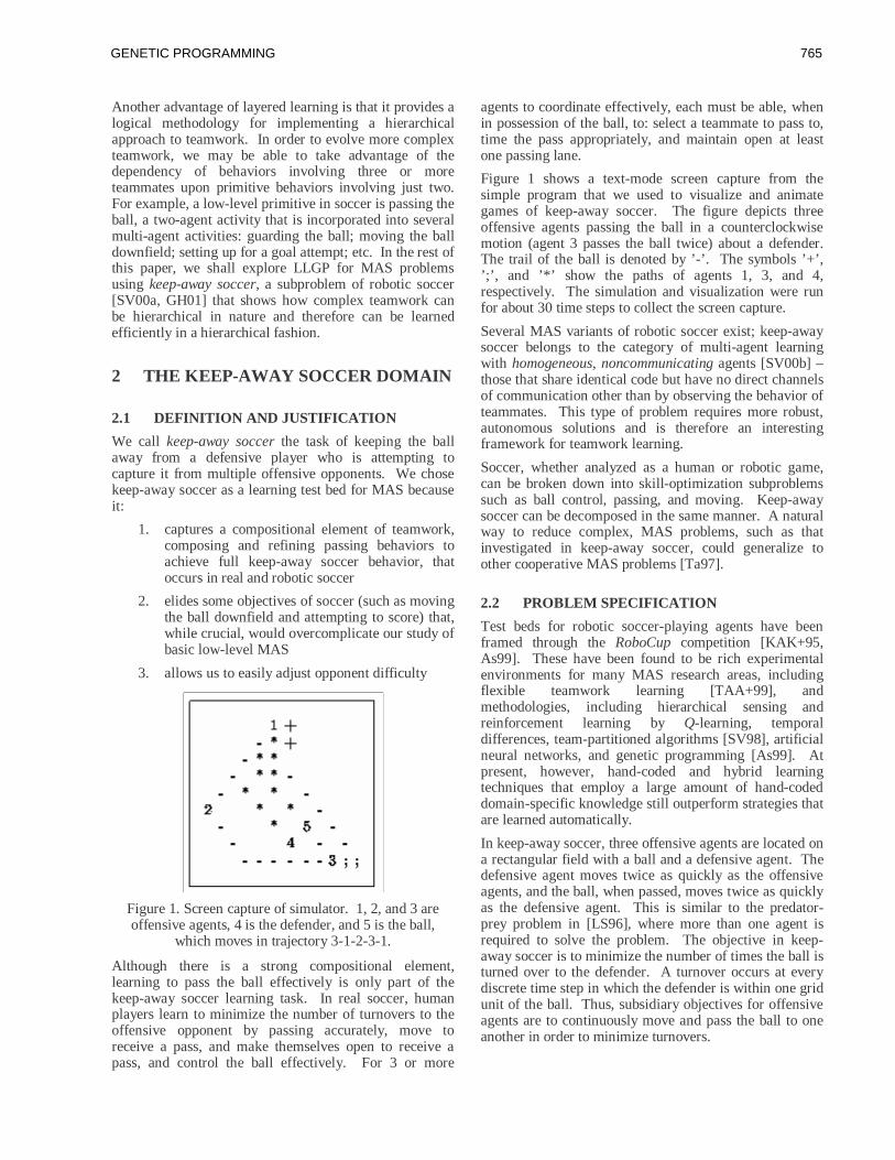
Another advantage of layered learning is that it provides alogical methodology for implementing a hierarchicalapproach to teamwork. In order to evolve more complexteamwork, we may be able to take advantage of thedependency of behaviors involving three or moreteammates upon primitive behaviors involving just two.For example, a low-level primitive in soccer is passing theball, a two-agent activity that is incorporated into severalmulti-agent activities: guarding the ball; moving the balldownfield; setting up for a goal attempt; etc. In the rest ofthis paper, we shall explore LLGP for MAS problemsusing keep-away soccer, a subproblem of robotic soccer[SV00a, GH01] that shows how complex teamwork canbe hierarchical in nature and therefore can be learnedefficiently in a hierarchical fashion.

2 THE KEEP-AWAY SOCCER DOMAIN

2.1 DEFINITION AND JUSTIFICATION

We call keep-away soccerthe task of keeping the ballaway from a defensive player who is attempting tocapture it from multiple offensive opponents. We chosekeep-away soccer as a learning test bed for MAS becauseit:

1. captures a compositional element of teamwork,composing and refining passing behaviors toachieve full keep-away soccer behavior, thatoccurs in real and robotic soccer

2. elides some objectives of soccer (such as movingthe ball downfield and attempting to score) that,while crucial, would overcomplicate our study ofbasic low-level MAS

3. allows us to easily adjust opponent difficulty

Figure 1. Screen capture of simulator. 1, 2, and 3 areoffensive agents, 4 is the defender, and 5 is the ball,

which moves in trajectory 3-1-2-3-1.

Although there is a strong compositional element,learning to pass the ball effectively is only part of thekeep-away soccer learning task. In real soccer, humanplayers learn to minimize the number of turnovers to theoffensive opponent by passing accurately, move toreceive a pass, and make themselves open to receive apass, and control the ball effectively. For 3 or more

agents to coordinate effectively, each must be able, whenin possession of the ball, to: select a teammate to pass to,time the pass appropriately, and maintain open at leastone passing lane.

Figure 1 shows a text-mode screen capture from thesimple program that we used to visualize and animategames of keep-away soccer. The figure depicts threeoffensive agents passing the ball in a counterclockwisemotion (agent 3 passes the ball twice) about a defender.The trail of the ball is denoted by ’-’. The symbols ’+’,’;’, and ’*’ show the paths of agents 1, 3, and 4,respectively. The simulation and visualization were runfor about 30 time steps to collect the screen capture.

Several MAS variants of robotic soccer exist; keep-awaysoccer belongs to the category of multi-agent learningwith homogeneous, noncommunicatingagents [SV00b] –those that share identical code but have no direct channelsof communication other than by observing the behavior ofteammates. This type of problem requires more robust,autonomous solutions and is therefore an interestingframework for teamwork learning.

Soccer, whether analyzed as a human or robotic game,can be broken down into skill-optimization subproblemssuch as ball control, passing, and moving. Keep-awaysoccer can be decomposed in the same manner. A naturalway to reduce complex, MAS problems, such as thatinvestigated in keep-away soccer, could generalize toother cooperative MAS problems [Ta97].

2.2 PROBLEM SPECIFICATION

Test beds for robotic soccer-playing agents have beenframed through theRoboCup competition [KAK+95,As99]. These have been found to be rich experimentalenvironments for many MAS research areas, includingflexible teamwork learning [TAA+99], andmethodologies, including hierarchical sensing andreinforcement learning by Q-learning, temporaldifferences, team-partitioned algorithms [SV98], artificialneural networks, and genetic programming [As99]. Atpresent, however, hand-coded and hybrid learningtechniques that employ a large amount of hand-codeddomain-specific knowledge still outperform strategies thatare learned automatically.

In keep-away soccer, three offensive agents are located ona rectangular field with a ball and a defensive agent. Thedefensive agent moves twice as quickly as the offensiveagents, and the ball, when passed, moves twice as quicklyas the defensive agent. This is similar to the predator-prey problem in [LS96], where more than one agent isrequired to solve the problem. The objective in keep-away soccer is to minimize the number of times the ball isturned over to the defender. A turnover occurs at everydiscrete time step in which the defender is within one gridunit of the ball. Thus, subsidiary objectives for offensiveagents are to continuously move and pass the ball to oneanother in order to minimize turnovers.


We think of keep-away soccer as consisting of two layersof behavior: passing accurately with no defensive agentpresent, and moving and passing with a defender tominimize the number of turnovers that occur during agame. The two layers of behaviors come from a human-like view of soccer, but are not heavily dependent upondomain knowledge. Both types of behavior are importantto playing good keep-away soccer, but the operationaldefinition does not necessarily give us a way to measurethe effectiveness of a team of agents who have just playedkeep-away soccer, which would be useful for finding afitness function.

Next, we present the application of layered learning to GPand explain further how the keep-away soccer is a good,illustrative test bed for LLGP.

3 LAYERED LEARNING

Layered learningis a term used in the machine learningand intelligent agents literature [St00, SV00a] to describea task-driven and often incremental approach to acquiringhierarchies of behaviors by reinforcement learning.

de Garis [De90] introduced a very similar concept that hecalled behavioral memoryfor a genetic algorithm thatencoded neural networks. Weights and signs of thenetworks evolved for one behavior were used to constructa new population, evolved for a second behavior. Someof the initial network persisted in the solutions for the newbehavior. Schoenauer and Xanthakis [SX93] then laterapplied this concept for constrained genetic algorithmoptimization.

Harvey et al [HHC94] used a layered, incrementallearning approach to robot control in a vision-basednavigation system. The authors achieved this bysequentially evolving a population using a range of targetsfrom simple to complex. Winkeler and Manjunath[WM98] and Eriksson [Er00] later analyzed this approachtoward incremental learning.

Dorigo et al [DC97] developed another hierarchicallearning system that is somewhat different from layeredlearning as we have adapted it. In this method, inputs andprocessing elements are organized into a hierarchy (fromsimple to complex), each of whose layers is incrementallytrained and frozen. This is similar to previous workapplied in domains such as robot soccer, but is notidentical to layered learning or behavioral memory asthese methods do not arrest learning in a particularportion of the hierarchical model.

Applying the layered learning paradigm to a problemconsists of breaking that problem up into a hierarchy ofsubproblems. The original problem is then solvedsequentially, by using the learning results from all themember problems of each layer in the next layer. This isconceptually similar to many other divide-and-conquerlearning paradigms, but a key difference is that thestructure of thesolutiondoes not necessarily reflect thisprocedural hierarchy oftraining. For example, programs

evolved for a subtask in LLGP are used to seed an initialpopulation for the next layer, but they may not beincorporated verbatim in the overall solution as ADFs are.This type of hierarchical solution is different from thetype that ADF-based GP learning proposes to find, whichfocuses on code reuse and structure rather than on howthe subtasks are learned.

Problems that attempt to achieve human-competitivebehaviors [Ko98], such as robotic soccer and keep-awaysoccer, lend themselves well to bottom-up decomposition.This is because human task learning, especially ofcooperative multi-agent behavior, often occurs in abottom-up fashion where individuals or small groups firstlearn smaller tasks, then how to compose and coordinatethem to solve larger tasks. When the problem is of thistype and we are already using a biologically motivatedmethod such as GP, it seems very natural to use a bottom-up decomposition of the problem that simulates thisaspect of human learning and allows GP to learn each ofthe smaller problems.

Table 1 is a variant of the table found in [SV00a], whichwe have adapted to correlate each prerequisite of layeredlearning with a property of genetic programming forkeep-away soccer.

Table 1: Requirements for using layered learning and GPkeep-away soccer justifications.

Layered Learning Genetic Programming

1. Learning from rawinput is not tractable

Complex MAS problemsfor GP need to be definedat multiple levels ÿ

2. A bottom-updecomposition is given

MAS learning task iscompositional ÿ

3. Learning occursindependently at eachlevel

GP can be applied to eachlayer independently ÿ

4. The output of onelayer feeds the nextlayer’s input

The population in the lastgeneration of one layer isused as the next layer’sinitial population ÿ

When we modify standard GP for layered learning, weneed to develop a learning objective for each layer, i.e.,the fitness at each layer that selects ideal individualsforthe subtask. As seen in [Lu98], using a single-objectivefitness value often leads to the best performance, and ismuch easier than trying to define multi-objective fitnessfunctions. While multi-objective fitness functions shouldallow GP to evolve more complex behaviors, it becomesmore difficult to decide what the components of fitnessshould be and how important each one is to the solution.In preliminary experiments, we found that it wasinfeasible to develop either a set of Pareto optimizationcriteria or a weighted function over multiple objectivesfor keep-away soccer. Instead, we chose to focus on


automatically discovering how to composepassing agentsinto keep-away soccer agents.

Another issue we addressed for layered learning in GP isthe transfer of the population from the last generation ofprevious layer to the initial population of the next. Theideal team will consist of individuals with high fitness onthe coordinated MAS task. Meanwhile, in everypopulation, there are certain individuals that have a betterfitness than others. We might therefore consider copyingthat best individual only and seeding the entire initialpopulation of the subsequent layer with it. However, thisduplication removes the diversity that was evolved in theprevious layer, which may be detrimental because the bestindividual on the subtask may be a suboptimal problemsolver for the overall coordinated team activity. Thus, wedesigned two experiments using LLGP: one thatduplicates the best individual and one that simply copiesthe entire population.

The final issue we address for LLGP is learning-speedimprovement: to what degree can layered learningsimplify the learning problem, allowing the target fitnessto be reached faster than with standard GP? This increasein the slope of the learning-speed curve [Ka95] is to bedistinguished from speed-up learning, wherein theefficiency of the learned problem solver is improved. Weshow how layered intermediate and team fitnessobjectives achieve greater learning-speed than amonolithic fitness objective in the keep-away soccer testbed. We also demonstrate a technique for empiricallychoosing a point at which to stop learning primitive MASbehaviors and switch to the high-level MAS behavior.

4 GP AND EXPERIMENT DESIGN

We designed four initial GP experiments to investigateand benchmark the performance of LLGP: standard GP(SGP), GP with ADFs (ADFGP), LLGP with the bestindividual duplicated to fill initial populations (LLGP-Best), and LLGP with the entire final population of thefirst layer used to seed the next (LLGP-All ). SGP andADFGP use the singlemonolithic (i.e., non-layered)fitness function of minimizing the number of turnoversthat occur in a simulation. ADFGP allows each tree forkicking and moving to have two additional trees thatrepresent ADFs, where the first ADF can call the second,and both have access to the full function set available forSGP. LLGP-Best and LLGP-All both have two layers;the fitness objective for the first layer is to maximize thenumber of accurate passes (a two-agent task evaluatedover teams of three copies of the same individual, on thesame size field as the keep-away soccer task), whilefitness objective for the second layer is to minimize thenumber of turnovers.

We developed two variations on each experiment, withmaximum generation values of 51 and 101. The stoppingcriterion for both variations is achieved when an idealfitness measure of 0 (where fewer turnover turns arebetter) is found, or the maximum generation is reached.

Our preliminary experiments indicated that a populationsize of 2000 yielded good results for the keep-awaysoccer domain using both SGP and ADFGP. We alsofound that the 101-generation SGP achieved betterconvergence in fitness and individual size and the 51-generation SGP, with negligible fitness improvement after101 generations.

The genetic crossover operator generates 90 percent of thenext generation; tournament selection generates the other10 percent. [Ko92] The tournament size is 7, withmaximum depth 17. Table 2 summarizes the terminal setused, consisting of vectors that are egocentric, or relativeto the agent whose tree is being evaluated. Table 3summarizes the function set used, where all functionsoperate on and return vectors. Both sets are similar tothose used in [Lu98] and [AT99].

Table 2: Keep-away soccer terminals (egocentric vectors)

Terminal Description

Defender Vector to opponent

Mate1 Vector to first teammate

Mate2 Vector to second teammate

Ball Vector to ball

Table 3: Keep-away soccer function set

Function(arguments) Description

Rotate90(1) Rotate current vector 90 degreescounter-clockwise

Random(1) New random vector with magnitudebetween 0 and current value

Negate(1) Reverse vector direction

Div2(1) Divide vector magnitude by 2

Mult2(2) Multiply vector magnitude by 2

VAdd(2) Add two vectors

VSub(2) Subtract two vectors

IFLTE(4) if ||v1|| < ||v2|| thenv3 elsev4

The GP system we use was developed by Luke and iscalled Evolutionary Computation in Java (ECJ) [Lu00].The simulator we developed for keep-away soccerabstracts some of the low-level details of agents playingsoccer from theTeamBots[Ba01] environment, which inturn abstracts low-level details from theSoccerServer[An98] environment. Abstractions of this type allow thekeep-away soccer simulator to be incorporated later tolearn strategies for theTeamBots environment andSoccerServer.


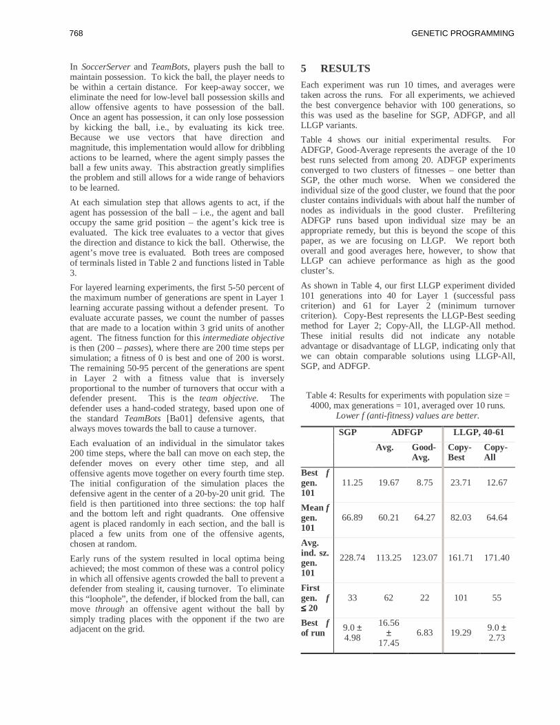
In SoccerServerand TeamBots, players push the ball tomaintain possession. To kick the ball, the player needs tobe within a certain distance. For keep-away soccer, weeliminate the need for low-level ball possession skills andallow offensive agents to have possession of the ball.Once an agent has possession, it can only lose possessionby kicking the ball, i.e., by evaluating its kick tree.Because we use vectors that have direction andmagnitude, this implementation would allow for dribblingactions to be learned, where the agent simply passes theball a few units away. This abstraction greatly simplifiesthe problem and still allows for a wide range of behaviorsto be learned.

At each simulation step that allows agents to act, if theagent has possession of the ball – i.e., the agent and balloccupy the same grid position – the agent’s kick tree isevaluated. The kick tree evaluates to a vector that givesthe direction and distance to kick the ball. Otherwise, theagent’s move tree is evaluated. Both trees are composedof terminals listed in Table 2 and functions listed in Table3.

For layered learning experiments, the first 5-50 percent ofthe maximum number of generations are spent in Layer 1learning accurate passing without a defender present. Toevaluate accurate passes, we count the number of passesthat are made to a location within 3 grid units of anotheragent. The fitness function for thisintermediate objectiveis then (200 –passes), where there are 200 time steps persimulation; a fitness of 0 is best and one of 200 is worst.The remaining 50-95 percent of the generations are spentin Layer 2 with a fitness value that is inverselyproportional to the number of turnovers that occur with adefender present. This is theteam objective. Thedefender uses a hand-coded strategy, based upon one ofthe standardTeamBots[Ba01] defensive agents, thatalways moves towards the ball to cause a turnover.

Each evaluation of an individual in the simulator takes200 time steps, where the ball can move on each step, thedefender moves on every other time step, and alloffensive agents move together on every fourth time step.The initial configuration of the simulation places thedefensive agent in the center of a 20-by-20 unit grid. Thefield is then partitioned into three sections: the top halfand the bottom left and right quadrants. One offensiveagent is placed randomly in each section, and the ball isplaced a few units from one of the offensive agents,chosen at random.

Early runs of the system resulted in local optima beingachieved; the most common of these was a control policyin which all offensive agents crowded the ball to prevent adefender from stealing it, causing turnover. To eliminatethis “loophole”, the defender, if blocked from the ball, canmove through an offensive agent without the ball bysimply trading places with the opponent if the two areadjacent on the grid.

5 RESULTSEach experiment was run 10 times, and averages weretaken across the runs. For all experiments, we achievedthe best convergence behavior with 100 generations, sothis was used as the baseline for SGP, ADFGP, and allLLGP variants.

Table 4 shows our initial experimental results. ForADFGP, Good-Average represents the average of the 10best runs selected from among 20. ADFGP experimentsconverged to two clusters of fitnesses – one better thanSGP, the other much worse. When we considered theindividual size of the good cluster, we found that the poorcluster contains individuals with about half the number ofnodes as individuals in the good cluster. PrefilteringADFGP runs based upon individual size may be anappropriate remedy, but this is beyond the scope of thispaper, as we are focusing on LLGP. We report bothoverall and good averages here, however, to show thatLLGP can achieve performance as high as the goodcluster’s.

As shown in Table 4, our first LLGP experiment divided101 generations into 40 for Layer 1 (successful passcriterion) and 61 for Layer 2 (minimum turnovercriterion). Copy-Best represents the LLGP-Best seedingmethod for Layer 2; Copy-All, the LLGP-All method.These initial results did not indicate any notableadvantage or disadvantage of LLGP, indicating only thatwe can obtain comparable solutions using LLGP-All,SGP, and ADFGP.

Table 4: Results for experiments with population size =4000, max generations = 101, averaged over 10 runs.

Lower f (anti-fitness) values are better.

ADFGP LLGP, 40-61SGP

Avg. Good-Avg.

Copy-Best

Copy-All

Best fgen.101

11.25 19.67 8.75 23.71 12.67

Mean fgen.101

66.89 60.21 64.27 82.03 64.64

Avg.ind. sz.gen.101

228.74 113.25 123.07 161.71 171.40

Firstgen. f≤≤≤≤ 20

33 62 22 101 55

Best fof run 9.0±

4.98

16.56±

17.456.83 19.29 9.0±

2.73


Table 5: Results for different Layer 1 durations(population size = 2000), averaged over 10 runs.


Layer 2Start

Generation

FirstGen.f ≤≤≤≤ 20

FirstGen.f ≤≤≤≤ 15

Best fGen.101

Best fof Run

5 62 79 12 11.75

10 18 30 11.4 9.7

15 24 43 9.63 9.38

20 38 47 9.6 9.6

25 47 80 11.88 11.25

30 51 58 14.1 12.7

35 46 55 7.75 7.25

40 57 82 13.6 13.2

45 67 93 14.11 13.11

50 62 82 11.5 11.1

We hypothesized that we were not yet realizing the fullimprovement in learning-speed that could be achievedusing LLGP. To test this hypothesis, we plotted the Layer2 learning-speed curves [Ka95] shown in Table 5 andFigure 1 for the following LLGP-All configurations: 5generations in Layer 1 and 96 in Layer 2, 10 and 91, up to50 and 51. The 10-91, 15-86, and 20-81 versions ofLLGP-All achieve better convergence than those that startLayer 2 later, except for 35-66. Even accounting for the“early start”, we can see that the convergence rate is fasterand the final fitness is better for LLGP when Layer 1 lastsbetween 10 and 20 generations. We ran a second series ofLayer 2 learning-speed curves (6 through 15, step 1) thatindicated that the learning rates for 10 through 15 werenot significantly different. We have not yet evaluated theinherent benefit to generalization quality – i.e., overfittingcontrol and reusability – of stopping Layer 1 earlier,

though this may be a good question for futureexperimentation.

A population size of 2000 is used for the fitness curves, asthe performance for 2000 is similar to that for 4000, asreported in [Gu00]. Note that if the learning-speed curvefor Layer 1 duration of 0 were plotted in Figure 2 above,it would be equivalent to that of the SGP, because theSGP runs for 101 generations with only the teamobjective function (Layer 2 fitness).

Table 6: Results for experiments with population size =4000, max generations = 101, averaged over 10 runs.


SGP Good-ADFGP

LLGP-All,10-91

Best fgen. 101 11.25 8.75 9.43

Mean fgen. 101 66.89 64.27 70.39

Avg.ind. sz.gen. 101

228.74 123.07 249.21

1st gen.f ≤≤≤≤ 20 33 22 26

Best f ofrun 9.0± 4.98 6.83 5.78± 2.28

Having found that the 10-91 LLGP exhibited a betterlearning speed curve, we repeated the LLGP-Allexperiment with population size 4000 and found that itwas able to match the Good-ADFGP performance,converged at least as quickly as any other GP, andresulted in the lowest best-of-run fitness values we found(fewer than 6 turnovers per simulation). This result isshown in Table 6, with the SGP and Good-ADFGP resultsrepeated for comparison. We note that the Layer 2individuals are much larger for LLGP-All-10-91 than forLLGP-All-40-61. That is, while stopping Layer 1 earlyyields a slight improvement in overall fitness and asignificant improvement in learning-speed, it does notnecessarily result in a more streamlined agent code. Thisis intuitive because more learning is deferred to Layer 2,where “passing” behavior is incorporated into the moresophisticated “keep-away” agents.

6 CONCLUSIONSWe have shown that using layered learning, geneticprogramming can evolve intelligent agents for acooperative MAS task such as keep-away soccer morequickly, with better fitness. Additionally, layeredlearning GP allows for a natural decomposition of theMAS learning problem into subproblems, each of whichis more easily solved with GP. The keep-away soccerproblem is a good test bed for abstracting away the

Learning-Speed Curves (5-50, Step 5)

0

10

20

30

40

50

60

70

80

90

100

1 7 13 19 25 31 37 43 49 55 61 67 73 79 85 91 97

Generation

Bes

tfitn

ess

5101520253035404550

Figure 2. Layer 2 learning-speed curves (eachstarting at the end of Layer 1) for different Layer 1

durations. Lower is better.


complexities of simulated soccer and allows for differentGP methods to be evaluated and their relative meritscompared. It is also easily extended to the full game ofrobotic soccer, and is highly portable across platformsbecause our simulator,TeamBots[Ba01], SoccerServer[An99], andECJ [Lu00] are all written in Java.

Conceptually, we can liken our success with LLGP to thesuccess of human soccer teams. Successful teams areusually made up of players with unique strategies, wherelearning took place in a bottom-up fashion and individualsfirst learned to play well together in pairs and smallgroups, then as a coordinated team. The LLGP-Allexperiments simulate this kind of behavior, where weattempt to minimize the number of generations needed perlayer. Our results indicate that layered learning in GPyields benefits over both standard GP and over hand-coded hierarchical approaches that depend on a largevolume of domain knowledge. This is because it is easierand more natural to use the team fitness function to derivean intermediate fitness function, evolve primitive MASagents, then let the higher-level (Layer 2) GP discoverhow to compose and refine primitive MAS behavior intocomplex MAS behavior.

We have considered several extensions to this research.First, developing a full-scale team for theRoboCupcompetition using LLGP would be a good way to test itsabilities more thoroughly (however, the focus in thispaper was on evaluating MAS task decomposition andimprovement of learning accuracy and learning speed).Diversity in populations is also an interesting issue, andour continuing research in LLGP investigates how andwhether LLGP promotes diversity. A related question isthe degree to which LLGPreusescode versusrefining itin higher layers. Other interesting modifications includedeveloping heterogeneous teams, adding additional lower-and higher-level layers, and hybridizing ADFs andlayered learning GP.

Acknowledgments

Support for this research was provided in part by theArmy Research Lab under grant ARL-PET-IMT-KSU-07and by the Office of Naval Research under grantsN00014-00-1-0769 and N00014-01-1-0917. We alsothank Edmund Burke for providing support for the secondauthor in continuing this work. Finally, thanks to SeanLuke for providing help with ECJ, the GP library used todevelop our system.

References

[An99] D. A. Andre. SoccerServer Manual Ver. 4, Rev.02. Available through the World-Wide Web athttp://www.robocup.org, 1999.

[As99] M. Asada. Overview of RoboCup-98. InRoboCup-98: Robot Soccer World Cup II (Lecture Notesin Artificial Intelligence Vol. 1604). Springer-Verlag,New York, NY, 1999.

[AT99] D. A. Andre and A. Teller. Evolving TeamDarwin United. In RoboCup-98: Robot Soccer WorldCup II (Lecture Notes in Artificial Intelligence Vol. 1604).Springer-Verlag, New York, NY, 1999.

[Ba01] T. Balch. TeamBotssoftware and documentation.Available through the World-Wide Web athttp://www.teambots.org, 2001.

[De90] H. deGaris. Genetic Programming: BuildingArtificial Nervous Systems Using GeneticallyProgrammed Neural Network Modules". In B. W. Porteret al, editors,Proceedings of the Seventh InternationalConference on Machine Learning (ICML-90), p. 132-139,1990.

[DC97] M. Dorigo and M. Colombetti.Robot Shaping:An Experiment in Behavior Engineering. MITPress/Bradford Books, 1997.

[Er00] R.I. Eriksson. An initial analysis of the ability oflearning to maintain diversity during incrementalevolution. In A. A. Freitas, editor,Data Mining withEvolutionary Algorithms, p. 120-124. 2000.

[HHC94] I. Harvey, P. Husbands, and D. Cliff. Seeingthe light: artificial evolution, real vision. In D. Cliff et al,editors,From Animals to Animats 3: Proceedings of theThird International Conference on Simulation of AdaptiveBehavior. MIT Press/Bradford Books, Boston MA, 1994.

[GH01] S. M. Gustafson and W. H. Hsu. LayeredLearning in Genetic Programming for A CooperativeRobot Soccer Problem. In J. F. Milleret al, editors,Proceedings of the European Conference on GeneticProgramming (EuroGP-2001). Lake Como, Italy.Springer-Verlag, 2001.

[Ka95] C. M. Kadie. Seer: Maximum LikelihoodRegression for Learning-Speed Curves. Ph.D.Dissertation, University of Illinois at Urbana-Champaign(Technical Report UIUC-DCS-R1874). August, 1995.

[KAK+95] H. Kitano, M. Asada, Y. Kuniyoshi, I. Noda,and E. Osawa. RoboCup: The Robot World CupInitiative. In Proceedings of the 1995 International JointConference on Artificial Intelligence (IJCAI-95)Workshop on Entertainment and AI/Alife. Montréal,Canada, 1995.

[Ki97] H. Kitano. The RoboCup Synthetic AgentChallenge 97. In Proceedings of the1997 InternationalJoint Conference on Artificial Intelligence (IJCAI-97),Nagoya , Japan, 1997.

[Ko92] J. R. Koza. Genetic Programming: On theProgramming of Computers by Means of NaturalSelection. MIT Press, Cambridge, MA, 1992.

[Ko94] J. R. Koza. Genetic Programming II: AutomaticDiscovery of Reusable Programs. MIT Press, Cambridge,MA, 1994.

[Ko98] J. R. Koza.Genetic Programming III: DarwinianInvention and Problem Solving. Morgan Kaufmann, LosAltos, CA, 1998.


[LS96] S. Luke and L. Spector. Evolving Teamwork andCoordination with Genetic Programming. InGeneticProgramming 1996: Proceedings of the First AnnualConference. J. Kozaet al, eds. p. 141-149. MIT Press,Cambridge, MA, 1996.

[Lu98] S. Luke. Genetic Programming ProducedCompetitive Soccer Softbot Teams for RoboCup-97. InProceedings of the Third Annual Genetic ProgrammingConference (GP98). J. Koza et al, eds. p. 204-222.Morgan Kaufmann, Los Altos, CA, 1998.

[Lu00] S. Luke. Issues in Scaling Genetic Programming:Breeding Strategies, Tree Generation, and Code Bloat.Ph.D. Dissertation, Department of Computer Science,University of Maryland, College Park, MD, 2000.

[MNH97] H. Matsubara, I. Noda, K. Hiraku. Learning ofCooperative Actions in Multi-agent Systems: A CaseStudy of Pass Play in Soccer. InAdaptation, Coevolution,and Learning in Multiagent Systems: Papers from the1996 American Association for Artificial Intelligence(AAAI) Spring Symposium, AAAI Technical Report SS-96-01, p. 63-67. AAAI Press, Menlo Park, CA, 1996.

[RB94] J. P. Rosca and D. H. Ballard. Hierarchical Self-Organization in Genetic Programming. InProceedings ofthe Eleventh International Conference on MachineLearning (ICML-94), p. 251-258. Morgan Kaufmann,Los Altos, CA, 1994.

[St00] P. Stone. Layered Learning in MultiagentSystems: A Winning Approach to Robotic Soccer.MITPress, Cambridge, MA, 2000.

[SV98] P. Stone and M. Veloso. A Layered Approach toLearning Client Behaviors in the RoboCup Soccer Server.Applied Artificial Intelligence (AAI) 12(3):165-188.Taylor and Francis, London, UK, 1998.

[SV00a] P. Stone and M. Veloso. Layered Learning. InProceedings of the Eleventh European Conference onArtificial Intelligence (ECAI). 2000.

[SV00b] P. Stone and M. Veloso. Multiagent Systems: ASurvey from a Machine Learning Perspective.Autonomous Robots, 8(3): 345-383. Kluwer AcademicPublishers, Norwell, MA, 2000.

[SVR99] P. Stone, M. Veloso, and P. Riley. TheCMUnited-98 Champion Simulator Team. InRoboCup-98: Robot Soccer World Cup II (Lecture Notes inArtificial Intelligence Vol. 1604). Springer-Verlag, NewYork, NY, 1999.

[SX93] M. Schoenauer and S. Xanthakis. Constrained GAOptimization. In S. Forrest, editor,Proceedings of theFifth International Conference on Genetic Algorithms(ICGA-93), p. 573-580. Morgan Kaufmann, San Mateo,CA, 1993.

[Ta97] M. Tambe. Towards Flexible Teamwork.Journalof Artificial Intelligence Research, 7: 83-124, 1997.

[TAA+99] M. Tambe, J. Adibi, Y. Alonaizon, A. Erdem,G. Kaminka, S. Marsella, and I. Muslea. Building Agent

Teams using an Explicit Teamwork Model and Learning,Artificial Intelligence, 110:215-240. Elsevier, 1999.

[WM98] J.F. Winkeler and B.S. Manjunath. IncrementalEvolution in Genetic Programming. In J.R. Koza, editor,Genetic Programming 1998: Proceedings of the ThirdAnnual Conference, p. 403-411. Morgan Kaufmann, SanMateo, CA, 1998.


Adaptive Hierarchical Fair Competition (AHFC) Model for

Parallel Evolutionary Algorithms

Jianjun Hu* [email protected]

Erik D. Goodman* [email protected]

Kisung Seo* [email protected]

Min Pei* [email protected]

Department of Computer Science and Engineering

Michigan State University East Lansing, MI 48824

*Genetic Algorithms Research and Applications Group Michigan State University

2857 W. Jolly Rd., Okemos, MI 48864

Abstract

The HFC model for parallel evolutionary computation is inspired by the stratified competition often seen in society and biology. Subpopulations are stratified by fitness. Individuals move from low-fitness to higher-fitness subpopulations if and only if they exceed the fitness-based admission threshold of the receiving subpopulation, but not of a higher one. The HFC model implements several critical features of a competent parallel evolutionary computation model, simultaneously and naturally, allowing rapid exploitation while impeding premature convergence. The AHFC model is an adaptive version of HFC, extending it by allowing the admission thresholds of fitness levels to be determined dynamically by the evolution process itself. The effectiveness of the Adaptive HFC model is compared with the HFC model on a genetic programming-based evolutionary synthesis example.

1 INTRODUCTION Parallel evolutionary algorithms (PEA’s) have gained increasing attention in many large-scale application problems including graph-partitioning problems, set partitioning problems, and many commercial efforts in analog circuit synthesis at Analog Design Automation Co. (Liang, 2001), Neolinear Inc (Ochotta, 1996; Krasnicki, 1999) and Genetic Programming Inc. (Andre, 1996). Parallel evolutionary computation models can be largely categorized into three classes (Cantu-Paz, 1998; Nowostawski, 1999): (1) global single- population master-slave models (2) single-population fine grained models, and (3) multi-population coarse-grained (or island) models. As cluster computing and networked PC's

have become available in many companies, multi-population parallel models (sometimes combined with master-slave models) have become increasingly popular. Parallel evolutionary algorithms have major advantages over single-population models, including parallel evaluation and rapid exploration with decreased risk of premature convergence. However, current parallel EA's are still not competent vis-a-vis scalability, either with respect to increasing degree of difficulty of the problem or to speedup with an increasing number of processors. It is clear that a competent parallel evolutionary algorithm should have the capability to:

(1) quickly exploit high-fitness individuals as they are discovered. One of these mechanisms is Elitism, which is effective in preserving good individuals, as has been demonstrated in several of the most successful evolutionary multi-objective optimization algorithms, such as NSGAII and SPEAII (Zitzler, 2000).

(2) keep multiple high-fitness individuals simultaneously to facilitate exploration in multiple search areas or directions

(3) maintain diversity of the population to avoid premature convergence

(4) be scalable with respect to increasing number of processors

(5) adapt its parameters for autonomous evolutionary computation.

Multi-population PEA’s can be classified into homogeneous models and heterogeneous models. Sprave (1999) proposed a unified model of population structures in PEAs, but his model doesn’t concern with the heterogeneity of the sub-populations. In homogeneous parallel EA models, each subpopulation is regarded as playing the same role in evolution. Homogeneous PEA’s often lack efficient mechanisms to exploit the newly discovered high-fitness individuals. Although they may keep several high fitness individuals in different demes,


they suffer from the fact that high-fitness individuals may easily dominate all subpopulations by means of the exchange (“migration”) process. Heterogeneous parallel EA’s are typically more resistant to this phenomenon. For example, the injection island GA (iiGA) (Lin, 1994; Eby, 1999) uses a hierarchical structure, typically stratifying subpopulations according to the level of resolution of the representation, allowing control of the tradeoff between low-resolution exploration and high-resolution exploitation. The iiGA has also been used with different fitness functions in various subpopulations, even if they used the same problem representation. Aickelin (1999) also proposed such a PEA, which he called a pyramidal EA, in which the hierarchical structure of the subpopulations is defined by a hierarchy of fitness functions.

In a recent paper (Hu and Goodman, 2002), we proposed the Hierarchical Fair Competition (HFC) model for parallel evolutionary computation. The HFC model is inspired by the observation of a strategy employed in some societal and biological systems to maintain different high-fitness individuals in a whole population. HFC turns out to have the features of a competent PEA cited above except the adaptability of (6). In this paper, we introduce an adaptive version of the HFC model, in which the admission thresholds are automatically determined and adjusted in the evolutionary process. In Section 2, the metaphor and the HFC model are described relative to the above features. In Section 3, an adaptive mechanism for determining the parameters of the HFC model is presented, along with the algorithm. We apply the AHFC model to a genetic programming problem and compare it with the static HFC model in Section 4. The conclusions and discussion are provided in Section 5.

2 THE HIERARCHICAL FAIR COMPETION MODEL (HFC) FOR PARALLEL EVOLUTION

2.1 MOTIVATION AND BACKGROUND OF HFC

The HFC model originates from an effort to combat the premature convergence phenomenon in traditional genetic algorithms and genetic programming. In a traditional GA, as the evolutionary process goes on, the average fitness of the population gets higher and higher, so that new individuals tend to survive only if they have similarly high fitness. New “explorer” individuals in fairly different regions of the search space usually have low fitness, until some local exploration and exploitation of their beneficial characteristics has occurred. So a standard EA tends to concentrate more and more of its search effort near one or more early-discovered peaks, and to get “stuck” near these attractors (or local optima). It is clear that in a standard EA, there exists a severely unfair competition. That is, selection pressure makes high-fitness individuals reproduce quickly and thus

supplant other individuals with lower fitness, some of which may lie in the vicinity of the global optimum, when if their neighborhood were explored more thoroughly, much higher-fitness individuals would be found. This fact holds true even when we find search points near a global optimum, as long as they are not close enough to have high fitness relative to those near other, earlier-explored local optima. This “unfair” competition contributes a lot to the slow search progress of many EA’s when confronted with difficult, high- dimensionality, multi-modal problems. To address this unfair competition problem, we need allow young but promising individuals (i.e., those in relatively newly-found regions, which may ultimately give rise to high-fitness offspring, but which are currently not of high fitness) to “grow up” and, at an appropriate time, join in the cruel competition process and be kept for further exploitation or be killed (as appropriate) when they are demonstrated with some confidence to be bad. At the same time, we hope to maintain the already-discovered high-fitness individuals and select from them even more promising individuals for exploitation without killing younger individuals. Following the tradition of getting inspiration from biology, we find that in some societal and biological systems, there exists an efficient mechanism that can maintain and foster potentially-high-fitness individuals (or, more accurately, potential progenitors of high-fitness individuals) efficiently. This is the hierarchical fair competition (HFC) principle as discussed below.

2.2 THE METAPHOR OF HFC: HIERARCHICAL FAIR COMPETITION IN SOCIETAL AND BIOLOGICAL SYSTEMS

Competition is widespread in societal and biological systems, but diversity remains large. After close examination, we find there is a fundamental principle underlying many types of competition in both societal and biological systems: the Fair Competition Principle.

2.2.1 The Fair Competition Principle in Societal Systems

In human society, competitions are often organized into a hierarchy of levels. None of them will allow unfair competition – for example, a young child will not normally compete with college students in a math competition. We use the educational system to illustrate this principle in more detail.

In the education system of China and many other developing countries, primary school students compete to get admission to middle schools and middle school students compete for spots in high schools. High school students compete to go to college and college students compete to go to graduate school (Fig. 1) (in many Western countries, this competition starts at a later level, but is eventually present, nonetheless). In this hierarchically structured competition, at each level, only individuals of roughly equivalent ability will participate


in any competition; i.e., in such societal systems, only fair competition is allowed. This hierarchical competition system is an efficient mechanism to protect young, potentially promising individuals from unfair competition, by allowing them to survive, learn, and grow before joining more intense levels of competition. Individuals that “lose” in these fair competitions were selected against while competing fairly only against their peers. Students compete fairly against others in their grade level because they are usually of similar absolute fitness levels, having been exposed to similar amounts of education and experience.

An interesting phenomenon sometimes found in societal competitions is the “child prodigy.” A ten-year-old child may have some extraordinary academic ability. These prodigies may skip across several educational levels and begin to take college classes at a young age. An individual with sufficient ability (fitness) is allowed to join any level of competition. This also suggests that in subpopulation migration, we should migrate individuals according to their fitness levels, rather than according to “time in grade.”

With such a fair competition mechanism that exports high-fitness individuals to higher-level competitions, societal systems reduce the prevalence of unfair competition and the unhealthy dominance or disruption that might otherwise be caused by “early-achieving” individuals.

2.2.2 The Fair Competition Principle in Biological Systems

It is somewhat surprising that in “cruel” biological/ ecological systems, the fair competition principle also holds in many cases. For example, there are mechanisms that reduce unmatched or unfair competition between young animals and mature ones. Among mammals, young individuals often compete with their siblings under the supervision of parents, but not directly with other mature individuals, since their parents protect them against other

adults. When the young grow up enough, they leave their parents and join the competition with other mature individuals. Evolution has found the mechanisms of parental care and sibling competition to be useful in protecting the young and allowing them to grow up and develop their full potentials. Fair competition seems to be beneficial to the evolution of many species.

2.3 THE HFC MODEL

Inspired by the fair competition principle and the hierarchical organization of competition within subpopulations in societal systems, we propose the Hierarchical Fair Competition parallel model (HFC), for genetic algorithms, genetic programming, and other forms of evolutionary computation.

A cadem iclevel

Figure 1: In education system s, lowlevel students com pete to get

adm ission to higher level schools.

prim aryschool

middleschool

highschool

college

graduateschool

Figure 2: HFC model extends the search horizontally insearch space and vertically in fitness dimension and kills

bad individuals at appropriate times while allowingpromising young individuals grow up continuously

level 0

level 1

level 2

level 3

level 4

fitness

Figure 3: In HFC model, subpopulations are organized ina hierarchy with ascending fitness levels. Each level (with

one or more subpopulations) accomodates individualswithin a certain fitness range determined by the admission

thresholds

fitness

fmin

fmaxsubpop9

subpop8

subpop7

subpop5,6

subpop3,4

subpop0,1,2

ADT5

AdmissionBuffers

randomindividuals

ADT:AdmissionThreshold

ADT4

ADT3

ADT2

ADT1


In this model (Fig 3), multiple subpopulations are organized in a hierarchy, in which each subpopulation can only accommodate individuals within a specified range of fitness. The entire range of possible fitnesses is spanned by the union of the subpopulations’ ranges. Conceptually, each subpopulation has an admission buffer that has an admission threshold determined either initially (fixed) or adaptively. The admission buffer is used to collect qualified candidates, synchronously or asynchronously, from other subpopulations. Each subpopulation also has an export threshold (fitness level), defined by the admission threshold of the next higher-level subpopulation. Only individuals whose fitnesses are between the subpopulation’s admission threshold and export threshold are allowed to stay in that subpopulation. Otherwise, they are exported to the appropriate higher-level subpopulation. Exchange of individuals is allowed only in one direction, from lower-fitness subpopulations to higher-fitness subpopulations, but migration is not confined to only the immediately higher level.

Each subpopulation can have the same or different sizes, operators, and other parameters. However, considering that there are often more low-fitness peaks than high-fitness peaks, we tend to allocate larger population sizes or more subpopulations to lower fitness levels, to provide extensive exploration; and we tend to use higher selection pressures in higher-fitness-level subpopulations to ensure efficient exploitation. As it is often easier to make a big fitness jump in a lower level subpopulation, we often end up using larger fitness ranges for low-level subpopulations, and smaller ranges for high-level subpopulations (Fig. 2), but, of course, that depends on the properties of the fitness landscape being explored. The critical point is that the whole range of possible fitnesses must be spanned by the union of the ranges of all levels of subpopulations. Of course, the highest-level subpopulation(s) need no export threshold (unbounded above) and the lowest-level subpopulation(s) need no admission threshold (unbounded below).

Exchange of individuals can be conducted synchronously after a certain interval, or asynchronously, as in many parallel models. At each moment of exchange, each individual in each subpopulation is examined, and if it is outside the fitness range for its subpopulation, it is exported to the admission buffer of a subpopulation with an appropriate fitness range. When a new candidate is inserted into an admission buffer, it can be inserted into a random position or inserted by sorting (or a null buffer may be used, inserting migrants directly into the receiving subpopulation, using some replacement rule). After export, each subpopulation imports the appropriate number of qualified candidates from its admission buffer into its pool. Subpopulations (especially at the base level) fill any spaces still open after emptying their admission buffers by generating new individuals at random to fill the spaces left by the exported individuals.

The number of levels in the hierarchy or number of subpopulations (if each level has only one subpopulation) can be determined initially or adaptively. In the static HFC model, we must manually decide into how many levels the fitness range will be divided, the fitness thresholds, and all other GA parameters. In a dynamic HFC model, we can dynamically change the number of levels, number of subpopulations, size of each subpopulation, and admission and export fitness thresholds. As will be seen below, a benefit of the adaptive HFC model (an example of a dynamic HFC) is that it can adaptively allocate search effort according to the characteristics of the search space of the problem to be solved, thereby searching more efficiently (initial research on various methods for adaptation of thresholds is in preparation for reporting elsewhere). However, even “coarse” setting of the parameters in a static HFC model has yielded major improvement in search efficiency over current EA’s on example problems.

Another useful extension to HFC used here is to introduce one or more sliding subpopulations, with dynamic admission thresholds that are continually reset to the admission threshold of the level in which the current best individual has been found. Thus, these subpopulations provide additional search in the vicinity of the advancing frontier in the hierarchy.

2.3.1 HFC as a competent parallel model for parallel evolutionary computation

(1) While low-fitness individuals can persist long enough to allow thorough exploration, as soon as they produce high-fitness offspring, the offspring can advance to higher-fitness levels immediately for further exploitation, to compete and be recombined with other high-fitness individuals.

(2) The HFC model maintains a large number of high-fitness individuals in high-fitness-level subpopulations without threatening lower-fitness (but perhaps promising) individuals. Thus possibly promising new search locales can persist long enough to be appropriately exploited.

(3) HFC provides another mechanism for maintaining diversity. First, the diversity of the population is ensured by the stratification in the fitness space. Second, continuous introduction of random individuals into the lowest-level subpopulations and the promotion of their high-fitness offspring to upper-level subpopulations can be regarded as the introduction of entropy and randomness into the overall evolutionary system. Actually, looking from low-fitness levels to higher-fitness levels, we observe increasing order in the population. The HFC evolution is thus a self-organizing process in which the highest order is achieved at the top fitness level. This mechanism reduces the chance of HFC becoming “stuck” at local optima and helps it explore new search areas. HFC thus implements implicitly a


multi-start or re-initialization mechanism on a continual basis.

(4) The HFC model quickly captures superior offspring and moves them to a place where they are free to compete with, and be recombined with, each other. This produces an effect similar to the elitism often used in multi-objective evolutionary computation, such as NSGAII or SPEAII (Zitzler et al., 2000), in which superior individuals are also kept separately. At that level, we can control the intensity of selection to determine the tradeoff between exploitation of those high-fitness individuals and exploration in their neighborhoods.

(5) HFC has a good scalability to more processing hosts. As more processors are available, they can be distributed to different fitness levels – either to low-level subpopulations for more extensive exploration, or to the higher-level ones for intensive exploitation of high-fitness individuals.

One of the major difficulties in the HFC evolutionary algorithm is the determination of the admission thresholds for a given problem. As the fitness landscape is often unknown before evolutionary search, it is hard to define these admission thresholds initially. Considering that admission thresholds in HFC are only used to segregate the whole population to avoid unfair competition, the behavior of the search is generally not extremely sensitive to the values of these admission thresholds, so that it is not necessary to set them to exactly optimal values. The only requirement for these thresholds is that the union of the fitness level ranges (which is determined by these admission thresholds) span the entire range of possible fitnesses. Based on this analysis, we propose an automatic admission thresholds determination mechanism for HFC model.

3 THE ADAPTIVE HFC MODEL In the static HFC model, we need to determine the number of subpopulations, the number of fitness levels, the relationship of subpopulations to fitness levels and the admission thresholds of each fitness level. All the admission thresholds are determined based on some initial exploration of the fitness landscape of the problem, such as the range of the fitness or distribution of early-discovered peaks. The threshold adaptation mechanism proposed here enables us to be relieved from this prerequisite expertise in the problem space. All we must decide is the number of admission levels ( lN ).

Since in HFC, random individuals are continuously inserted into subpopulations of the base fitness level, the export threshold of the base fitness level can be set as the average fitness of the whole population after several (nCalibGen) generations. In AHFC, this is called the calibration stage, which determines the level of the fitness value of frequently encountered (“normal”) individuals with respect to random individuals. So the base level is used to export normal individuals to higher

levels for further exploitation. At the end of the calibration process, the standard deviation fσ and the max fitness maxf of individuals at the highest level, the average fitness fµ of individuals at the base level are calculated. Then the fitness range of each level can be calculated by the following formula:

Admission threshold of base level= -∞ (1)

Admission threshold of the first level = fµ (2)

Admission threshold of the highest fitness level =

maxf fσ− (3)

Admission thresholds of other fitness levels iL , are

determined by:

( )/( 2) 1,..., 1maxf L f f N i Ni f l lσµ µ+ × − − − = − (4)

Table 1: Adaptive Heterogeneous HFC Algorithm for Parallel EA’s

1. Initialization Determine EAP : parameters for standardmulti-population EA. (We assume here using one setof parameters for all subpopulations)

lN :Number of levels of the hierarchy nCalibGen: calibration generations nUpdateGen: admission threshold update

interval nExch: generations between admission process

exchanges gen = 1: current generation 2. Do

if gen < nCalibGen (in calibration stage) run EA without exchange else if gen = nCalibGen (calibration stage ends)

determine the admission thresholds for each level by formulas (1) - (4)

else if gen% nExch = 0 Do for each subpopulation from lowest level tohighest level {

Examine fitness of each individual andexport to corresponding subpopulation athigher level for which fitness rangeaccommodates this exported individual(replacing worst individual in targetsubpopulation)}

end do else if gen % nUpdateGen =0 update admission thresholds of all but the baselevel by (3), (4) gen ++

until the stopping criterion is satisfied. return the highest-fitness individual(s) from thehighest-level subpopulation

End


However, it is clear that as the evolutionary search goes on, higher-fitness individuals are continuously discovered that ruin the segregation by the above admission thresholds determined at the initial calibration stage. So a dynamic admission threshold updating mechanism is proposed here. After each nUpdateGen generations, the maximal fitness, maxf , and the fitness standard deviation of the top level sub-populations, fσ , are recomputed to determine the admission threshold of all the fitness levels except the base level and the first level, by (3) - (4).

To enable efficient search, the mapping relationship of sub-populations to all levels also needs to be adapted dynamically. It is obvious that at initial stage, as all individuals are randomly generated, these individuals usually have low fitness. So most of the subpopulations should belong to the base level. As higher-level individuals discovered, more subpopulations should be allocated to higher levels to exploit high-fitness individuals. The following scheme is used in this paper: firstly, all subpopulations are allocated to base level. After the calibration stage, subpopulations are then evenly allocated to each level. Extra subpopulations can be allocated to higher levels (if aggressive exploitation is desired) or to lower level (if intensive exploration is desired).

This AHFC algorithm works like a string. At the initial stage, it is quite compressed, but gradually, the string stretches to accommodate individuals with a larger range of fitness. The whole algorithm of AHFC is given in Table 1. For simplicity, we give the pseudo code only for the adaptive HFC model with synchronous exchanges (no buffers).

4 EXPERIMENTS The adaptive HFC model for Genetic Programming (HFC-GP) has been applied to a real-world analog circuit synthesis problem that was first pursued using GP with a static HFC (Hu, 2002). In this problem, an analog circuit is represented by a bond graph model (Seo, 2001; Fan, 2001) and is composed of inductors (I), resistors (R), capacitors (C), transformers (TF), gyrators (GY), and Sources of Effort (SE). Our task is to synthesize a circuit, including its topology and sizing of components, to achieve specified behavior. The objective is to evolve an analog circuit with response properties characterized by a pre-specified set of eigenvalues. By increasing the number of eigenvalues specified, we can define a series of synthesis problems of increasing difficulty, in which premature convergence problems become more and more significant when traditional GP methods are used.

Circuit synthesis by GP is a well-studied problem that generally demands large computational power to achieve good results. Since both topology and the parameters of a circuit affect its performance, it is easy to get stuck in the evolution process.

4.1.1 Experiments on an Analog Circuit Synthesis Problem

Four circuits with increasing difficulty are to be synthesized, with eigenvalue sets as specified in Table 2. Circuits were evolved with single-population GP, multiple-population GP, HFC-GP, and AHFC-GP. The GP parameter for the single-population GP is shown in cell (1,2) of Table 3. The GP parameters for the multi-population GP were the same as for the single-population GP, except that the total population is divided into subpopulations with sizes shown in cell (2, 2) of Table 3. A one-way ring migration topology was used.

The parameters for the HFC-GP were the same as for the multi-population GP, except that the ring migration was

replaced by the HFC scheme. The fitness admission thresholds were set based on our prior experience with such eigenvalue problems. In this problem, we defined a fitness admission threshold for each subpopulation (one subpopulation per level, in this case) as shown in cell (2, 3) of Table 3. Subpopulation 15 was used as a “sliding” subpopulation to aggressively explore the fitness frontier.

Table 3: Parameter Settings for GP

Parameters of

Single Population GP

Popsize: 2000 init.method = half_and_half init.depth = 3-6 max_nodes = 800 max_depth = 13 crossover rate = 0.9 mutation rate = 0.1 max_generation = 1000

Additional

Parameters of Multi-Population

GP

Number of subpopulations = 15; Size of subpop 2 to 14 = 100 size of subpop 1 = 300 size of subpop 15 = 400 migration interval = 10 generations migration strategy: migrate (copy) 10 best individuals to the next subpopulation in the ring to replace its 10 worst individuals

Additional Parametersof HFC-GP

admission_fitnesses of: subpop 1 = -100000.0 subpop 2 to 14: 0.65, 0.68, 0.72, 0.75, 0.78, 0.80, 0.83, 0.85, 0.87, 0.9, 0.92, 0.95 subpop 15 = varying

Additional Parameters of

AHFC-GP

nUpdateGen= nCalibGen = 10 nExch = 10 Nl =8

Table 2: Target Eigenvalues Problem 1: 6-eigenvalue problem

2 3 .3 , 7 .5 4 .5 , 3 .5 12 .0i i i+ + +− − −− − −

Problem 2: 8-eigenvalue problem 2 3 .3 , 7 .5 4 .5 , 3 .5 12 .0 , 3 .4 12 .0i i i i+ + + +− − − −− − − −

Problem 3: 10-eigenvalue problem 2 3.3 , 7.5 4.5 , 3.5 12.0 , 3.4 12.0 , 10.0 8.0i i i i i+ + + + +

− − − − −− − − − −Problem 4: 12-eigenvalue problem

2 3 .3 , 7 .5 4 .5 , 3 .5 12 .0 ,i i i+ + +− − −− − −

3 .4 12 .0 , 10 .0 8 .0 , 1 .5 3 .0i i i+ + +− − −− − −


The parameters of AHFC-GP were nearly identical to those of the HFC, except that we don’t need to determine the admission thresholds of each level.

The performances of the four approaches were assessed on four problems with increasing difficulty. Each experiment was run ten times, with the average of the results reported in Fig.4, where the four GP methods are indicated by OnePop: Single-population GP MulPop: multi-population GP (ring topology) HFC-GP: HFC model for GP AHFC-GP: Adaptive HFC model for GP

From Figure 4, it is impressive to see that in all four problems, both AHFC and HFC performed dramatically better than the other algorithms vis-à-vis best of run, and the improvement was more dramatic on the more difficult

problems. The superior performance at the initial generations may have resulted from the rapid exploitation of superior individuals, in a single subpopulation, in comparison to the ring parallel GA. Yet convergence in the HFC and AHFC was much slower than in the single- and multi-population GP runs. In fact, we observe relatively steady improvement during the runs for this set of problems. For the easier problems, the (dynamic) AHFC actually out-performed the (static) HFC slightly, in spite of the rich experience on this class of problems that was used for setting the HFC thresholds. The fact that the HFC ultimately surpassed the AHFC on the two harder problems indicates that there is room for improvement of the AHFC scheme used here. However, the fact that it is competitive with human-determined

0 100 200 300 400 5000

0.1

0.2

0.3

0.4

0.5

0.6

0.7

0.8

0.9

1

generation

Standardized fitness of Best Individual of run

OnePopMulPopHFC-GPAHFC-GP

a) 6-eigenvalue problem

0 100 200 300 400 500 6000

0.2

0.4

0.6

0.8

1

generation

stan

dard

fitn

ess


OnePopMulPopHFC-GPAHFC-GP

b) 8-eigenvalue problem

0 200 400 600 8000

0.2

0.4

0.6

0.8

1

generation

stan

dard

fitn

ess


OnePop MulPop HFC-GP AHFC-GP

c) 10-eigenvalue problem

0 200 400 600 800 10000

0.1

0.2

0.3

0.4

0.5

0.6

0.7

0.8

0.9

1

generation

stan

dard

fitn

ess


OnePop MulPop HFC-GP AHFC-GP

d) 12-eigenvalue problem

Figure 4. Fitness of Best Individual to Date vs. Generation: dashdot (OnePop), solid (MulPop), dashed (HFC)


static values based on prior experience shows that it is a step in a beneficial direction.

5 CONCLUSIONS AND FUTURE WORK Based on our analysis of the role of admission thresholds used in the HFC model and our experiments on a series of difficult, highly epistatic real-world problems, it has been demonstrated that the adaptive HFC model can work nearly as well as the original HFC model, and even better in some cases, without any prerequisite knowledge of the fitness landscape of the problem. The dynamic allocation of the subpopulations to fitness levels also improves the search efficiency. These adaptation mechanisms make our algorithm to be easily plugged into new problems without much parameter tuning. Our experiments demonstrated the effectiveness of the HFC and AHFC models in improving significantly both the search speed and the quality of the best solutions found compared with standard EAs.

This paper represents a first step toward autonomous parallel evolutionary computation based on the HFC model. The second step is the automation of the adaptive distribution of the computing resource among levels. We expect that the number of subpopulations, the number of fitness levels, the distribution of subpopulations to each level, along with the admission thresholds, can all be determined adaptively, in which case we would have an autonomous parallel evolutionary computation model in which the communication topology and migration scheme are all decided by the evolutionary process itself, according to the characteristics of the problem at hand.

In this paper, we implemented the synchronous version of the AHFC model and simulated parallel genetic programming on a single PC. More consideration about the communication cost and asynchronous adaptation mechanism of the AHFC model in the case of a large population is needed. The scalability of the AHFC model with respect to more processors also needs to be proved with experiments on real parallel cluster computing facilities, which is on the top of our task list.

Acknowledgment The authors acknowledge the assistance of Prof. Ronald C. Rosenberg and Zhun. Fan in defining and exploring the example problem presented here. This work was supported by the National Science Foundation under contract DMI 0084934.

References J.M. Liang; T. McConaghy; A. Kochlan; T. Pham; G. Hertz. “Intelligent Systems for Analog Circuit Design Automation: A Survey,” Proceedings World Multiconference on Systemics, Cybernetics and Informatics, Vol. IX. SCI 2001/ ISAS 2001, Orlando, Florida (USA), 2001.

E. S. Ochotta, R. A. Rutenbar, L. R. Carley, “Synthesis of High-Performance Analog Circuits in ASTRX/ OBLX,”

IEEE Trans. CAD, Vol. 15, pp. 273-294, Mar., 1996.

M. Krasnicki, R. Phelps, R. Rutenbar, and R. Carley. “Maelstrom: Efficient simulation-based synthesis for custom analog cells,” Proceedings of the 1999 ACM/IEEE Design Automation Conference, 1999.

D. Andre and J. R. Koza. “Parallel genetic programming on a network of transputers,” in Angeline, Peter J. and Kinnear, Kenneth E., Jr. (eds.), Advances in Genetic Programming, MIT Press, Cambridge, MA, 1996.

E. Cantu-Paz, “A survey of parallel genetic algorithms,” Calculateurs Parallels, 10(2), Paris, Hermes. 1998.

J. Sprave. A unified model of non-panmictic population structures in evolutionary algorithms. In P. J. Angeline and V. W. Porto, editors, Proc. 1999 Congress on Evolutionary Computation (CEC'99), vol 2, p. 1384-1391, Washington D.C., 1999. IEEE Press, Piscataway NJ.

N. Mariusz. and R. Poli, “Review and Taxonomy of Parallel Genetic Algorithms,” Technical Report, University of Birmingham, School of Computer Science, No. CSRP-99-11, May 1999.

S.C. Lin, E. Goodman, and W. Punch, “Coarse-Grain Parallel Genetic Algorithms: Categorization and New Approach,” IEEE Conf. on Parallel and Distrib. Processing, Nov., 1994.

D. Eby, R. C. Averill, E. Goodman, and W. Punch, “Optimal Design of Flywheels Using an Injection Island Genetic Algorithm,” Artificial Intelligence in Engineering Design, Analysis and Manufacturing, 13, p. 389-402, 1999.

U. Aickelin, “A Pyramidal Evolutionary Algorithm with Different Inter-Agent Partnering Strategies for Scheduling Problems,” Genetic and Evolutionary Computation Conference Late-Breaking Papers, E. Goodman, ed., ISGEC Press, San Francisco, pp. 1-8. 2001.

J.J. Hu, E.D. Goodman, “The Hierarchical Fair Competition (HFC) Model for Parallel Evolutionary Algorithms,” Proceedings of the 2002 Congress on Evolutionary Computation: CEC2002, (forthcoming), IEEE, Honolulu, Hawaii, 2002.

K. Seo, E. Goodman, and R. Rosenberg, “First Steps toward Automated Design of Mechatronic Systems Using Bond Graphs and Genetic Programming,” Proc. Genetic and Evolutionary Computation Conf. - 2001, July 7-11, Morgan Kaufmann, San Francisco, p. 189, 2001.

Z. Fan, J.J. Hu, K. Seo, E. Goodman, R. Rosenberg, and B. Zhang, “Bond Graph Representation and GP for Automated Analog Filter Design,” Genetic and Evolutionary Computation Conference Late Breaking Papers, pp. 81-86, 2001.

E. Zitzler, K. Deb, and L. Thiele, “Comparison of Multiobjective Evolution Algorithms: Empirical Results,” Evolutionary Computation, 8(2), pp. 173-195, 2000.


Structure Fitness Sharing (SFS) for Evolutionary Design by Genetic

Programming

Abstract

Balanced structure and parameter search is critical to evolutionary design with genetic programming (GP). Structure Fitness Sharing (SFS), based on a structure labeling technique, is proposed to maintain the structural diversity of a population and combat premature convergence of structures. SFS achieves balanced structure and parameter search by applying fitness sharing to each unique structure in a population, to prevent takeover by the best structure and thereby maintain the diversity of both structures and parameters simultaneously. SFS does not require definition of a distance metric among structures, and is thus more universal and efficient than other fitness sharing methods for GP. The effectiveness of SFS is demonstrated on a real-world bond-graph-based analog circuit synthesis problem.

1 INTRODUCTION Genetic programming has been applied successfully to a rich variety of problems such as machine code evolution (Nordin, 1997), quantum algorithm design (Spector, 1999), cellular automaton rule discovery, and soccer-playing program evolution (Andre 1999). GP has been particularly effectively used as an efficient Darwinian Invention Machine that enabled Koza et al. to achieve human-competitive results in analog circuit design and in the transmembrane segment identification problem (Koza 1999). Indeed, one of GP’s most significant features is the ability to simultaneously evolve both a structure and its parameters, opening up promising applications in many real-world engineering design problems and in neural network design. In all of these problems, the objective is to search for an open-ended structure, together with its related parameters, to achieve several desired goals. Genetic programming – especially evolutionary design by genetic programming – is recognized as making a high demand on computational

resources (Koza, 1999). To some extent, this demand can be traced to the premature convergence problem, especially convergence of the structures in a GP population; it can be ameliorated using diversity- maintenance techniques for the population. Based on an analysis of the weak causality of GP, the new concept of Structure Fitness Sharing (SFS), based on a structure labeling technique, is proposed to achieve balanced structure and parameter search by maintaining the diversity of both structures and parameters at all times. This method does not require definition of a distance metric, and is thus very efficient compared to other fitness sharing methods. Its effectiveness is demonstrated on a real-world bond-graph-based analog circuit synthesis problem using GP.

2 THE DIVERSITY PROBLEM IN EVOLUTIONARY DESIGN BY GP

2.1 CATEGORIES OF EVOLUTIONARY DESIGN PROBLEMS

Most evolutionary design problems can be classified into one of three types:

TYPE I: Fixed structure with fixed number of parameters.

These problems are essentially parameter optimization problems – the task is to optimize the parameters of a given structure. Genetic algorithms, simulated annealing, evolutionary programming, evolution strategies, and even gradient-based optimization techniques are often used here.

TYPE II: Variable structure with no parameters.

This type includes problems such as algorithm design, program induction and logic design, in which only structure search is needed. These problems are well suited for GP, which intrinsically manipulates the program structure, often represented as a tree. Of course, some of these problems can be solved with

Jianjun Hu+, Kisung Seo+, Shaobo Li*, Zhun Fan+, Ronald C. RosenbergΨ, Erik D. Goodman+ [email protected]

+Genetic Algorithms Research and Applications Group (GARAGe)

Michigan State University East Lansing, MI, 48824

*CAD Institute Guizhou University of Technology

Guiyang, 550003, China

ΨDepartment of Mechanical Engineering Michigan State University East Lansing, MI, 48824


genetic algorithms, simulated annealing, and other techniques, by using a somewhat indirect representation of the structure.

TYPE III: Variable structure with variable number of parameters (of course, there can also be variable structure with a fixed number of parameters, but that is not the typical case – number of parameters usually varies with the size of the structure).

Many of the most interesting evolutionary design problems belong to this third category, in which a structure is sought within a topologically open-ended space, but the fitness of a structure can often only be evaluated after parameters are assigned to key variables associated with the structures evolved. Since the structure is varied during the search process, the number of parameters and their semantics change frequently. Such problems include analog circuit design (Koza, 1999), mechanical system design (Fonseca, 1993), and neural network design (Oliker, 1992). Although a GA with a variable-length representation can be used here, GP, with its outstanding capability to search simultaneously for a good structure and for appropriate parameters, distinguishes itself as the most important tool for this kind of open-ended design problem.

2.2 PREMATURE CONVERGENCE AND DIVERSITY IN THREE TYPES OF EVOLUTONARY DESIGN PROBLEMS

TYPE I problems are often described as parameter optimization problems, readily addressable by GA. Premature convergence in GA has been well studied. Common diversity maintenance techniques include crowding (DeJong, 1975), deterministic crowding (Mahfoud, 1992), and fitness sharing (Goldberg, 1989). The fitness derating method (Beasley, 1993), a multi-objective method, employs fitness sharing in a popular and effective way.

The premature convergence problem when GP is applied to TYPE II problems has also been well studied. Most of the resulting methods are derived from GA, but with some specific consideration of the GP context. In multi-objective genetic programming, Rodriguez (Rodriguez-Vazquez, 1997) uses the MOGA approach with fitness sharing being performed in the fitness space, and extends it to genetic programming. Though easier to implement, it remains an open question whether diversity of fitness values is generally a true indicator of the diversity of a population – a measure which should actually be based on the parameter space. DeJong et al. (DeJong, 2001) use the multi-objective method to explicitly promote diversity by adding a diversity objective. In their method, a distance measure defined as follows is used in the diversity objective. The distance between two corresponding nodes is zero if they are identical and one if they are not. The distance between two trees is the sum of the distances of the corresponding

nodes – i.e., distances between nodes that overlap when the two trees are overlaid, starting from the root. The distance between two trees is normalized by dividing by the size of the smaller of the two trees. The diversity objective is defined as the average squared distance to other members of the population. An improved version of the above distance metric between two trees is proposed in Ekart and Nemeth (2000) and used to do fitness sharing in GP. Their method includes the following three steps:

1) The two GP trees to be compared are brought to the same tree-structure (only the contents of the nodes remain different).

2) The distance between each pair of symbols situated at the same position in the two trees is computed.

3) The distances computed in the previous step are combined in a weighted sum to form the distance of the two trees.

The major improvement of this method is that it differentiates the types of nodes when calculating the distance between two nodes. It first divides the GP functions and terminals into several subsets. For nodes with types belonging to the same subset, it calculates the relative distance. For nodes with types belonging to different subsets, it uses a defined function to make sure that the distance between nodes from different subsets is larger than that between nodes of the same subset. It also considers the fact that a difference at some node closer to the root could be more significant than a difference at some node farther from the root, using a multiplier K to distinguish them. Edit distance and phenotypic distance for fitness sharing for GP are also tested in their experiment. The former gets slightly better accuracy but with relatively high computational cost. The latter doesn’t provide much improvement over the original GP without fitness sharing.

Implicit fitness sharing (McKay, 2000) has also been applied to GP. Instead of calculating the distance between the structures of GP trees, it is a kind of phenotypic (behavior-based) fitness sharing method. The fitness is “shared” based on the number of other individuals who have similar behaviors, capabilities or functions. Implicit fitness sharing provides selection pressure for each individual to make different predictions from those made by other individuals.

Population diversity of TYPE III problems in GP has not been investigated thoroughly. These problems are characterized by the need for simultaneous optimization of topology and parameters. In a GP population, structure diversity is needed to enable efficient topology exploration, which is the main objective, in most case, for discovery of innovative designs. At the same time, the goodness (or fitness) of a structure can only be evaluated after sufficient parameter exploration within the same structure. Thus, the parameter diversity of each structure also needs to be maintained. As a result, in the context of variable structure and parameter design by GP, the


population diversity has some significant differences from that of a GA, in the following respects:

• Number of peaks

When applying fitness sharing in GA, two assumptions are made. One is that the number of peaks is known or can be estimated. The second is that the peaks are almost evenly distributed. In many problems of GA, a relatively limited number of peaks is expected to enable efficient use of fitness sharing. However, in TYPE III problems, each structure may have a huge number of peaks with respect to its parameter space, while in the structure space, each structure is a distinct peak, since the structure space is not a continuous space, but rather a highly nonlinear discrete space.

• Continuity of search space

In GA, many problems can be considered as defined in an approximately continuous space, although sometimes certain aspects have distinctly discrete behavior. However, in TYPE III problems, GP deals with a highly discrete structure space that also has a huge continuous space (of parameter values), since for each structure, the search for appropriate parameters can be regarded as an instance of GA search.

• Constraints

In GA, only parameter constraints exist. However, in TYPE III problems, GP must deal with both structure constraints and parameter constraints.

The demand for structure diversity as well as parameter diversity makes the existing fitness sharing methods inefficient for Type III problems. For fitness-space-based fitness sharing (Rodriguez-Vazquez, 1997) and the implicit fitness sharing (McKay, 2000) methods, significant parameter diversity is lost since they do not promote coexistence of individuals with the same structure but with different parameters in order to enable efficient parameter search. Fitness sharing with the distance metric, as in (Ekart, 2000; KeJong, 2001), is also inefficient in this case. First, the computational cost is still demanding, since in TYPE III problems, a complex structure and its parameters often require a big tree – perhaps 1000 - 2000 nodes in most of our experiments – especially when parameters are normally represented by a numeric subtree such as Koza uses (Koza, 1999). Second, but more importantly, the underlying assumption of the above distance metrics is that structural dissimilarity measured between two GP trees meaningfully reflects the dissimilarity in function between the two structures. However, as the structure space represented by a GP tree is a highly non-linear space, in most cases, a change of a single (non-parameter) node changes the behavior of the GP tree dramatically. This phenomenon can be traced to the weak causality of GP (Rosca, 1995), which means that

small alterations in the underlying structure of a GP tree cause big changes in the behavior of the GP tree. So measuring a sort of "Hamming" distance between the structures of two GP trees to predict the difference of the behavior/function is not well founded, and thus inefficient. This makes a useful definition of a sharing radius hard to determine. It seems that distance metrics in the structure space and the parameter space and the association of a set of parameters with the structure to which they apply must be faithfully captured in order to most effectively maintain both structure diversity and parameter diversity and thereby to achieve efficient search. Therefore, given the inherent difficulty of structure/function mapping, perhaps it is counterproductive to use any structural similarity measure beyond the most basic and completely faithful one – the identity mapping: two structures are either identical, or they are not. That is the structural distance measure used here. While it is possible to define a broader relationship that still captures identity of function (for example, if swapping of the order of two children of a node has no effect on the function computed), such definitions depend on the semantics of the functions, and were not implemented here.

3 BALANCED STRUCTURE AND PARAMETER SEARCH IN EVOLUTIONARY DESIGN BY GP

In design problems involving both variable structure and variable parameters, search must be balanced between the structure and parameters. On one hand, each structure needs sufficient exploration of its parameters to develop its potential to some extent, which means that a reasonable number of individuals of the same structure must probably be kept in the population. On the other hand, no structure should dominate the population, or it would prevent sufficient future exploration of the structure space.

Premature convergence of structures in evolutionary design by GP can be caused by neglecting the different roles of structure and parameter search. In standard GP, nodes at which to perform crossover and mutation are selected randomly from the entire set of nodes, treating those specifying structure modifications identically with those specifying numerical modifications (provided that numerical subtrees are used to define the parameters of components, as is often done). This means that a new circuit structure is often discarded by the selection process if its fitness is low with its initial set of parameters. The result is that often, structures of moderate quality with slightly better parameters proliferate and dominate the population, while inherently better structures with bad parameters are discarded. This is called the premature structural convergence problem. This phenomenon arises from the fact that ’’promising’’ structures are often discarded just because their current parameters are not adjusted well enough to demonstrate their potential. Ideally, a structure should be discarded only when it is demonstrated to be bad after a sufficient effort to adjust its


parameters. In addition, since there are often many more numeric nodes than structure modifying nodes, premature structural convergence is accentuated, since there is a lower probability of choosing a structure modifying node that will generate a new structure than of choosing a node that changes only parameters.

In order to address this problem, structure and parameter search must be controlled explicitly. In our work, a probabilistic method is first devised to decide whether GP does a structure modification (crossover or mutation on a structure modifying node) or does parameter modification (crossover or mutation on a parameter modifying node). Since structure changes have a more fundamental effect than the parameter changes on the performance of the system, we introduce a bias toward more parameter modifications than structure modifications by controlling the probability of selecting these types of nodes for crossover and mutation sites. The following example probabilities are defined to facilitate keeping the structure and its function stable and to allow parameters to be adjusted well enough to demonstrate the potential of a structure.

We also use explicit control of the node selection process to achieve balanced parameter evolution for all parameters in a structure. During the parameter modification stage, we first establish a list of all variables whose values need to be established during evolution, then we randomly select a variable as the current variable to be changed. We then select a node in the numeric subtree of this variable and do a crossover or mutation operation. In this way, each variable has an equal opportunity to be changed during evolution. This improvement speeds the evolution of balanced numeric subtrees. All variables tend to have numeric subtrees with similar depths.

Even with the methods above, premature structural convergence still often occurs as structures with well-fitted parameters quickly dominate the whole population. The Structure Fitness Sharing (SFS) method is proposed to control the reproduction of high-fitness structures. Our assumptions are that fitness sharing can profitably be based on the number of individuals with the same structure, and that distance between the structures of two GP trees with distinct structures is not generally an adequate predictor of the differences between their behaviors. Thus, any “counting of positions where the trees differ” distance metric is not well founded. Instead, a simple labeling technique is used to distinguish structures.

4 STRUCTURE FITNESSS SHARING (SFS)

Structure Fitness Sharing is the application of fitness sharing to structures in GP. In contrast to the GA fitness sharing using a distance measure to identify peaks, in SFS, fitness sharing is based on the tree structures, treating each tree structure in GP as a peak in the space of parameters and structures.

In SFS, each structure is uniquely labeled, whenever it is first created. So long as GP operations on an individual do not change its structure, but only its parameters, the structure label of this individual is not changed. Parameter crossover and mutation, or replication of the individual, simply increase the number of individuals with this structure (label) in the population. If structure modifications are conducted on an individual that change the structure – for example, we change a Rep_C (a GP function node replacing a resistor or inductor of the circuit with a capacitor) to a Rep_I (a GP function replacing a resistor or capacitor of the circuit with an inductor) node – then a new structure label (structureID) is created and is attached to this new individual. Our assumption is that the possibility that any particular structure-altering operation produces exactly the same structure possessed by other individuals in the current population is relatively low, so it is not necessary (or worthwhile) to check a new structure against all other existing structures to see if it is identical with one of them (and so could use its label), although a hashing technique might make this relatively easy to do. Furthermore, even if some newly created individual shares the same structure with another individual but is labeled with a different structure label, the algorithm is not strongly affected, so long as it occurs infrequently.

In standard GP, individuals with certain structures will prosper while others will disappear because of their low fitnesses. If this process is allowed to continue without control, some good structures (usually one) tend to dominate the population and premature convergence occurs. To maintain diversity of structures, fitness sharing is applied to individuals of each structure. SFS decreases the fitness of the individual as follows: SFS penalizes only those structures having too many individuals, according to the following fitness adjustment rule used for the experiments in this paper:

sN : Number of structures to be searched simultaneously

espN : Expected number of search points (individuals) for each structure in the whole population

: Number of individuals with structure is (of which individual iind is one)

For each individual iInd if then

( ) 0.1( ) 0.9

p structure modificationp parameter modification

==

i iInd s

siN∈

0.8*i i

esp

Ind s

si NN∈

>


where α =1.5

If 1 1.0k then k> =

With this method, each structure has a chance to do parameter search. Premature convergence of structures is limited, and we can still devote more effort to high-fitness structure search.

4.1 LABELING TECHNIQUE IN SFS

A labeling technique is used in SFS to distinguish different structures efficiently. A similar technique has been used by Spears (1994), in which tag bits are used to identify different subpopulations. Spears’s result suggests that in crowding and fitness sharing in GA, we only need to decide whether or not two individuals have the same label. The added precision of the distance metric for maintaining the diverse state of a subpopulation is often unnecessary. In SFS, the label is used only to decide whether or not two individuals have the same label (i.e., structure). We use simple integer numbers as labels rather than more complicated tag bits. Ryan (1994, 1995) also uses similar labelling ideas to decide which race an individual belongs to in his racial GA (RGA).

4.2 HASH TABLE TECHNIQUE IN SFS

In order to keep track of all individuals with each particular label, SFS uses a hash table is used -- this speeds up the access to the structure by each individual when we do crossover, mutation, and reproduction. Each time we create a new structure, we create an entry in the hashtable with the structureID (next integer) as the key. The size of the hash table is controlled to accommodate at most 500 structures in our experiments. Whenever the number of structure entries in the hashtable exceeds 500, those structure entries with no individuals in the current population or with a low fitness of its best individuals and with old ages (generations since their labels were created) are removed from the hashtable. The corresponding individuals of these structures are removed from the current population at the same time.

4.3 THE STRUCTURE FITNESS SHARING ALGORITHM IN GP

The following is the outline of the algorithm of SFS as applied to GP:

Step 1: Initialize the population with randomly generated individuals. Initialize the structure hash table.

Step 2: Assign each individual a unique label. Here a label is just an unassigned integer number incremented by one at each assignment.

Step 3: Loop over generations

3.1 Select the parents for a genetic operation according to their standard fitness

3.2: If current operation is an operation that changes the structure from that of the parent(s), (including crossover and mutation at structure operator nodes of GP trees)

Create a new label for each new structure created and add the new structure item to the structure hash table.

3.3: If the current operation is a parameter modification (mutating the parameter nodes or crossing over at a parameter node) or only replication of an existing individual, do not create a new label. New individuals inherit the labels from their parents. Update information about the structure items in the hash table, including the best fitness of this structure, number of individuals, age, etc.

3.4: If the maximum number of structures in the hash table is reached, first purge those structures that have no individuals in the current population. If there are still too many structures, then delete those structures whose best individuals have lower fitness and high age (>10 generation, in our case) and delete their individuals in the population and replace them with new individuals formed by crossover or mutation until the maximum number of structures in hash table is kept.

3.5: Adjust the fitness of each individual according to equation (1).

Step 4: If stopping criterion is satisfied, stop; else go to step 3.

5 EXPERIMENTS

5.1 PROBLEM DEFINITION

GP with the SFS technique has been applied to an analog circuit synthesis problem that was previously approached using GP without SFS (Rosenberg, 2001). In this problem, an analog circuit is represented by a bond graph model (Fan, 2001) and is composed of inductors (I), resistors (R), capacitors (C), transformers (TF), gyrators (GY), and sources of effort (SE). The developmental evolution method similar to (Koza, 1999) is used to evolve both the structure and parameters of a bond graph representation of a circuit that achieves the user-specified behavior. With this method, a set of structure modifying operators (e.g. Rep_C, Rep_I) are provided to operate on the embryo

* (1)adj oldf f k=

Ind S

esp

ii i

sNk N

α

∈

−

=


bond graph. A set of numeric operators (such as +, -, *, /) are provided to modify the parameters of the structure.

In this paper, the design objective is to evolve an analog circuit with response properties characterized by a pre-specified set of eigenvalues of the system equation. By increasing the number of eigenvalues specified, we can define a series of synthesis problems of increasing difficulty, in which premature convergence problems become more and more significant when traditional GP methods are used. This eigenvalue assignment problem has received a great deal of attention in control system design. Control over eigenvalues in designing systems, in order to avoid instability and to provide particular response characteristics, is often an important and practical problem.

Circuit synthesis by GP is a well-studied problem that generally demands large computational power to achieve good results. Since both the topology and the parameters of a circuit affect its performance, it is easy to get stuck in the evolution process.

5.2 EXPERIMENTAL SETUP

In the example that follows, a set of target eigenvalues was given and a bond graph model with those eigenvalues was generated. Table 1 shows the three sets of 6, 8, and 10 target eigenvalues used as targets for example genetic programming runs:

We applied single population GP with and without SFS and multi-population GP with and without SFS to all three problem instances. Each experiment was repeated 10 times with different random seeds.

The embryo model used is shown in Figure 1. It represents an embryo bond graph with three initial modifiable sites (represented as dotted boxes). In each case, the fixed components of the embryo are sufficient to allow definition of the system input and output, yielding a system for which the eigenvalues can be evaluated, including appropriate impedances. The construction steps specified in the GP tree are executed beginning from this embryo. The numbers in parentheses represent the parameter values of the elements.

Three circuits of increasing complexity are to be synthesized, with eigenvalue sets as specified above. The GP parameter tableau for the single population method is shown in Table 2 below.

These problems exhibit a very high degree of epistasis, as a change in the placement of any pair of eigenvalues has a

strong effect on the location of the remaining eigenvalues. Eigenvalue placement is very different from “one-max” or additively decomposable optimization problems, and these problems become increasingly difficult with the problem order. The performance of each of the three GP approaches is reported in Figure 2, in which the four GP methods are indicated by

OneGP: single population GP, no SFS MulGP: multi-population GP, no SFS ONE.SFS: single population GP with SFS MULPOP.SFS: multi-population GP with SFS

To observe the effect of structure fitness sharing, we monitor the number of distinct structures in the experiments with and without SFS techniques. From Fig 2, one can see that Structure Fitness Sharing can significantly improve the performance for single population GP and also does better in multi-population GP,

Table 2. Parameter Settings for GP

Parameters of Single Population

GP

Popsize: 1000 init.method = half_and_half init.depth = 3-6 max_nodes = 1000 max_depth = 15 crossover rate = 0.9 mutation rate = 0.1 max_generation = 1000

Additional Parameters of

Multi-Population GP

Number of subpopulations = 10; Size of subpop = 100 migration interval = 10 generations migration strategy: ring topology, migrate 10 best individuals to the next subpopulation in the ring to replace its 10 worst individuals

SFS Parameters

sN : 50

espN : 20 = popsize/ sN

Table 1. Target Eigenvalues

Problem 1: 6-eigenvalue problem

0.1 5.0 , 1.0 2.0 , 2.0 1.0j j j− ± − ± − ±


0.1 5.0 , 1.0 2.0 , 2.0 1.0 , 3.0 0.7j j j j− ± − ± − ± − ±


0.1 5.0 , 1.0 2.0 , 2.0 1.0 , 3.0 0.7j j j j− ± − ± − ± − ±

4.0 0.4 j− ±

Figure 1. The Embryo Bond Graph Model


though the difference is not as significant. The reason may be that multi-population runs already provide an inherent diversity maintenance mechanism. We also find that SFS can help to provide probabilistic control of structure and parameter modifications to maintain a stable number of search structures in the whole population, as illustrated in Fig 3.

6 CONCLUSIONS

In this paper, Structure Fitness Sharing (SFS) is proposed to achieve balanced structure and parameter search in evolutionary design by Genetic Programming. SFS can effectively prevent the dominance of any specific structure and when combined with probabilistic control of structure and parameter modification, SFS can maintain a stable number of structures for simultaneous structure and parameter search. The labeling technique in SFS eliminates the necessity of computing the distance between two individuals, which saves computing effort that we believe is often largely wasted when attempting to measure GP structural similarity. The user parameters of the standard fitness sharing method are also eliminated (e.g. the sharing radius). All that must be done is to define the fitness adjustment scheme: how to penalize the fitness of a structure when the number of individuals with that structure label grows large enough to threaten the diversity of the population. The hash table technique allows SFS to quickly update the structure information about the current population during evolution. More complicated balanced structure parameter search methods can be derived using the concept of structure diversity. For example, the authors intend to incorporate the age concept and the elitism method of multi-objective evolutionary computation into SFS. We also intend to explore use of a separate GA for explicit exploration of the parameter spaces of individual structures, with the expectation of a significant impact on the selection, crossover and mutation dynamics of the overarching simultaneous evolutionary search of structure and parameters.

Acknowledgment

Thanks to Ahmad R Shahid for his assistance with the hash table technique. This work was supported by the National Science Foundation under contract DMI 0084934.

References:

P. Nordin, Evolutionary Program Induction of Binary Machine Code and Its Application, PhD thesis, University of Dortmund,Germany, 1997.

L. Spector, H. Barnum, and H. J. Bernstein, “Quantum Computing Applications of Genetic Programming”, Advances in Genetic Programming 3, L. Spector et al., eds., MIT Press, Cambridge, Mass., 1999, pp.135-160.

D. Andre and A. Teller, “Evolving Team Darwin United,"

RoboCup-98: Robot Soccer World Cup II. Lecture Notes in Computer Science, M. Asada and H. Kitano, eds., Vol. 164, Springer-Verlag, Berlin, pp.346-352, 1999.

J. R. Koza et al., Genetic Programming III: Darwinian Invention and Problem Solving, Morgan Kaufmann, San Francisco, 1999.

0 100 200 300 400 500 6000

0.2

0.4

0.6

0.8

1

generation

stan

dard

fitn

ess


ONEPOPONE.SFSMULPOPMULPOP.SFS

a) 6-eigenvalue problem

0 100 200 300 400 500 6000

0.2

0.4

0.6

0.8

1

generation

stan

dard

fitn

ess



b) 8-eigenvalue problem

0 100 200 300 400 500 6000

0.2

0.4

0.6

0.8

1

generation

stan

dard

fitn

ess



c) 10-eigenvalue problem

Figure 2. Fitness of Best Individual to Date vs. Generation


K. Rodriguez-Vazquez, C. M. Fonseca, and P. J. Fleming, "Multiobjective Genetic Programming : A Nonlinear System Identification Application," Proc. Genetic Programming '97 Conference, pp. 207-212, 1997

C. M. Fonseca, and P. J. Fleming, "Genetic Algoritms for Multiobjective Optimisation: Formulation, Discussion, and Generalization," Proceedings Fifth International Conference on Genetic Algorithms, Morgan Kaufmann, San Francisco, pp. 416-423, 1993.

S. Oliker, M. Furst, and O. Maimon, "A distributed genetic algorithm for neural network design and training," Complex Systems, 6, pp. 459-477, 1992.

K. A. DeJong. An Analysis of the Behavior of a Class of Genetic Adaptive Systems, PhD thesis. University of Michigan. Dissertation Abstracts International 36(10), 5410B. (University Microfilms No. 76--9381), 1975.

E. D. DeJong, R. A. Watson, and J. B. Pollack, "Reducing Bloat and Promoting Diversity using Multi-Objective Methods," Proc. GECCO-2001, Morgan Kaufmann, San Francisco, pp. 11-18.

S. W. Mahfoud, "Crowding and Preselection Revisited," Proc. PPSN-92, Elsevier, 1992.

D. E. Goldberg, Genetic Algorithms in Search, Optimization and Machine Learning, Addison Wesley, 1989.

D. Beasley, D.R. Bull, and R.R. Martin, "A Sequential Niche Technique for Multimodal Function Optimisation," Evolutionary Computation, 1, pp. 101-125. 1993.

A. Ekárt; S. Z. Németh, "A Metric for Genetic Programs and Fitness Sharing," in R. Poli, W. Banzhaf, W. B. Langdon, J. Miller, P. Nordin, T. Fogarty (eds.), Genetic Programming, Proceedings of EUROGP'2000, Edinburgh, 15-16 April 2000, LNCS volume 1802, pp. 259-270.

R. I. McKay, "Fitness Sharing in Genetic Programming," Proc. GECCO-2000, Las Vegas, NV, Morgan Kaufmann, San Francisco, July, 2000.

J. P. Rosca and D. H. Ballard, "Causality in Genetic Programming," in L. J. Eshelman, ed., Proc. Sixth International Conference on Genetic Algorithms, Morgan Kaufmann, San Francisco, pp. 256-263, 1995.

W. M. Spears, "Simple Subpopulation Schemes," Proc. Evolutionary Programming Conf., pp. 296-307, 1994.

C. Ryan, "Pygmies and Civil Servants, in K. E. Kinnear, Jr., ed., Advances in Genetic Programming, pp. 243-263. MIT Press, 1994.

C. Ryan, "Racial Harmony and Function Optimization in Genetic Algorithms - the Races Genetic Algorithm," in Proc. Of Evolutionary Programming 1995. pp. 296-307. MIT press.

R.C. Rosenberg, E. D. Goodman and K. Seo, "Some Key Issues in Using Bond Graphs and Genetic Programming for Mechatronic System Design", Proc. ASME

International Mechanical Engineering Congress and Exposition, 2001, November 11-16, New York.

Z. Fan, J. Hu, K. Seo, E. Goodman, R. Rosenberg, and B. Zhang, “Bond Graph Representation and GP for Automated Analog Filter Design,” Genetic and Evolutionary Computation Conference 2001 Late Breaking Papers, ISGEC Press, San Francisco, pp. 81-86.

0 100 200 300 400 500 6000

200

400

600

800

1000

generation

Num

ber o

f Stru

ctur

es in

the

who

le P

opul

atio

n

Control of structures in GP


a) 6 eigenvalue problem

0 100 200 300 400 500 600100

200

300

400

500

600

700

800

900

1000

generation

Num

ber o

f Stru

ctur

es in

the

who

le P

opul

atio

n



b) 8 eigenvalue problem

0 100 200 300 400 500 6000

200

400

600

800

1000

generation

Num

ber o

f Stru

ctur

es in

the

who

le P

opul

atio

n



c) 10 eigenvalue problem

Figure 3. Number of Structures in Population vs. Generation


Inference of Differential Equation Models by Genetic Programming

Hitoshi IbaGrad. School of Frontier Informatics,

The University of Tokyo7-3-1 Hongo, Bunkyo-ku, 113-8656, Japan

Erina SakamotoGrad. School of Inf. and Comm. Eng.,

The University of Tokyo7-3-1 Hongo, Bunkyo-ku, 113-8656, Japan

Abstract

This paper describes an evolutionary methodfor identifying a causal model from the ob-served time series data. We use a systemof ordinary differential equations (ODEs) asthe causal model. This approach is well-known to be useful for the practical applica-tion, e.g., bioinformatics, chemical reactionmodels, controlling theory etc. To explorethe search space more effectively in the courseof evolution, the right-hand sides of ODEsare inferred by Genetic Programming (GP)and the least mean square (LMS) method isused along with the ordinary GP. We applyour method to several target tasks and em-pirically show how successfully GP infers thesystems of ODEs.

1 Introduction

Ordinary differential equations (ODEs) are one of theeasiest media for modeling complex systems, wherebasic differential relationships are known between thesystem components. Solving a set of differential equa-tions to produce their equivalent functions is relativelyeasy so as to obtain useful time-series data. On theother hand, the inverse problem, i.e., the inference ofthe system of ODE from the observed time-series data,is not necessarily easy, although very important formany fields. This is because there is no knowing theappropriate form, i.e., the order and terms of ODEs,beforehand.

In this paper, we deal with an arbitrary form in theright-hand side of the system of ODEs to allow theflexibility of the model. More precisely, we considerthe following general form:

dXi

dt= fi(X1,X2, . . . ,Xn) (i = 1, 2, . . . , n), (1)

where Xi is the state variable and n is the number ofthe observable components.

For the sake of identifying the system, we use GeneticProgramming (GP) to evolve the ODEs from the ob-served time series. Although GP is effective in findingthe suitable structure, it is sometimes difficult to opti-mize the parameters, such as constants or coefficientsof the polynomials. This is because the ordinary GPsearches for them simply by combining randomly gen-erated constants. To avoid this difficulty, we introducethe least mean square (LMS) method.

There have been several studies for identifying differ-ential equation models by means of EAs (Evolution-ary Algorithms). For instance, GP was used to find afunction in a symbolic form, which satisfies the differ-ential equation and initial conditions [Koza92]. Caoand his colleagues used hybrid evolutionary model-ing algorithms [Cao00]. The main idea was to em-bed GA in GP, where GP was employed to discoverand optimize the structure of a model, while GAwas used to optimize its parameters, i.e., coefficients.[Babovic00] also applied GP to approximate severalODEs from the domain of ecological modeling, e.g.,Lotka-Volterra and logistic equations. They showedthat the GP-based approach introduced numerousadvantages over the most available modeling meth-ods. In our previous researches [Sakamoto and Iba00]and [Sakamoto and Iba01], we proposed another inte-grated scheme, in which the least mean square (LMS)method is used along with GP. In this scheme, someindividuals were created by the LMS method at someintervals of generations and they replaced the worstindividuals in the population.

In this paper, we extend our previous approach so


as to achieve the inference of the ODEs more effec-tively. More precisely, we empirically show the follow-ing points:

• The success in the acquisition of ODEs, which areclose to the observed time series.

• The inference of the exact equation form, i.e., theexact causal relationship.

• The effectiveness of the LMS method.• The superiority of our approach over the previousmethods.

The rest of this paper is organized as follows. In Sec-tion 2, we describe the details of our method, i.e., howGP and LMS methods are integrated to work in thecourse of evolution. Three examples are used to exam-ine the effectiveness of our method. Their experimen-tal results are shown in Section 3. Then, we discussthe results in Section 4 and give some conclusion inSection 5.

2 Integration of GP and LMS

We use GP to identify a causal model in the form ofthe system of ODEs. Though GP is capable of findinga desirable structure effectively, it cannot always beeffective in finding the proper coefficients because GPuses the combination of randomly selected ones. Wehave chosen the least mean square method (LMS) totackle this defect of the ordinary GP. For this purpose,coefficients are not included in the terminal set for aGP individual tree. The coefficients of each term ofa GP tree are calculated by the LMS method and atable of them composes a GP individual along with atree.

2.1 Inference of the form of equations usingGP

We use GP to identify the form of the system of dif-ferential equations. For this purpose, we encode right-hand sides of ODEs into a GP individual. Each in-dividual contains a set of n trees, i.e., an n-tuple oftrees(f1, . . . , fn). For example, consider the two treesin Fig.1. This shows the following system of ODEs:

{X1 = aX1X

22 + b

X2 = cX1X2 + dX2,(2)

where the coefficients a, b, c, d, are derived by LMS de-scribed later. Note that the constant term b is addedto the right hand side of the first equation, because of

the constant terminal, i.e., 1. Thus, each equation usesa distinct program. A GP individual maintains mul-tiple branches, each of which serves as the right-handside of a differential equation.

Crossover operations are restricted to the correspon-dent branch pairs. Actually, each tree, i.e., each righthand side of the ODE sytem, is evolved independentlyin parallel.

Figure 1: Example of a GP individual.

2.2 Optimization of models using LMSmethod

Coefficients of a GP individual is derived by the LMSmethod described below. Assume that we want toacquire the approximate expression in the followingform:

y(x1 , . . . , xL) =M∑

k=1

akFk(x1 , . . . , xL), (3)

where Fk(x1, . . . , xL) is the basis function, x1, . . . , xL

are the independent variables, y(x1, . . . , xL) is the de-pendent variable, and M is the number of the basisfunctions. Let a be the vector of coefficients, i.e.,(a1, . . . , aM ). Then, our purpose is to minimize χ2

described in (4) to acquire a.

χ2 =N∑

i=1

(y(i)−

M∑k=1

akFk(x1(i), . . . , xL(i)))2

, (4)

where x1(i), . . . , xL(i) and y(i) are data given for theLMS method and N is the number of data points. Letb be the vector of (y(1), . . . , y(N)) andA be theN×Mmatrix described below:

F1(x1(1), . . . , xL(1)) . . . FM (x1(1), . . . , xL(1))F1(x1(2), . . . , xL(2)) . . . FM (x1(2), . . . , xL(2))

.... . .

...F1(x1(N), . . . , xL(N)) . . . FM (x1(N), . . . , xL(N))


Then, (5) should be satisfied to minimize χ2.

(AT · A) · a = AT · b (5)

Thus, a can be acquired by solving this equation.

When applying to the time-series problem, y(i) for thejth equation of the system of differential equations iscalculated according to the following discrete differ-ence of the time-series xj(t):

y(i) = Xj |t=ti =xj(ti +∆t)− xj(ti −∆t)

2∆t, (6)

where ti is the time of the ith selected data point.For example, consider the first ODE (X1) of the sys-tem (2), in which the number of the components istwo (L = n = 2). In this case, we are using twobasis functions, i.e., M = 2 and (F1, F2)=(X1X

22 , 1).

Then, the ith row of the matrix A is determined as(x1(ti)x2(ti)2,1).

The coefficients in the approximate expressions of theright-hand sides of the equations can be derived byusing A and b(y(1), . . . , y(N)) acquired above.

2.3 Fitness definition

The fitness of each individual is defined as the sum ofthe squared error and the penalty for the degree of theequations:

fitness =n∑

i=1

T−1∑k=0

(x′i(t0+k∆t)−xi(t0+k∆t))2+a·m,

(7)

t0 : the starting time∆t : the stepsizen : the number of the observable componentsT : the number of the data points

where xi(t0+k∆t) is the given target time series (k =0, 1, · · · , T −1). x′

i(t0+k∆t) is the time series acquiredby calculating the system of ODEs represented by aGP individual. All these time series are calculated byusing the forth-order Runge-Kutta method. m is thenumber of terms and a is the weight constant. In otherwords, the individual which has a smaller number ofterms and is closer to the target time series has thehigher possibility to be selected and inherited to thenext generation. This fitness derivation is based on theMDL (Minimum Description Length) criterion, whichhas been often used in GP (see [Iba94], [Zhang95] and

Exp.1 Exp.2 Exp.3 Exp.4

Population size 1000 1000 1000 3000Generation 100 100 100 100Crossover rate 0.80 0.80 0.80 0.80Mutation rate 0.10 0.10 0.10 0.10# time series 1 1 3 3Stepsize 0.01 0.01 0.01# data points 100 40 30

Table 1: GP and LMS parameters for experiments.

[Nikolaev and Iba01] for examples). When calculatingthe time series, some individuals may go overflow. Inthis case, the individual’s fitness value gets so largethat it will be weeded out from the population.

We use several sets of time series as the training datafor GP. This is to acquire the equations as close to thetarget as possible. Each data set was generated fromthe same target by using different initial values.

3 Experimental results

We have prepared three different tasks to test the ef-fectiveness of our method. Experimental parametersare summarized in Table 1. Function and terminal setsF and T are as follows:

F = {+,−, ∗}T = {X1, . . . ,Xn, 1}

3.1 Example 1 : Chemical reaction model

The reaction between formaldehyde (X1) and car-bamide in the aqueous solution gives methylol urea(X2) which continues to react with carbamide andform methylene urea (X3) (see [Cao00] for details).The reaction equations are described as below:

HCHO + (NH2)2COk1−→ H2N · CO · NH · CH2OH

(8)

H2N · CO · NH · CH2OH + (NH2)2COk1−→ (NH2CONH)2CH2 (9)

As a kind of typical consecutive reaction, the concen-trations of the three components in the system satisfythe following system:

X1 = −1.4000X1

X2 = 1.4000X1 − 4.2000X2

X3 = 4.2000X2

(10)


Experimental parameters for this task are shown inTable 1. By applying our method, we have acquiredthe system of eq.(11), which gave the sums of squareerrors as (X1,X2,X3) = (0.000, 2.082 ∗ 10−11, 1.883 ∗10−11). The time series generated by this system isshown in Fig.2 along with that of the target.

X1 = −1.4000X1

X2 = 1.4004X1 − 4.2006X2

X3 = 4.1998X2

(11)

0

0.02

0.04

0.06

0.08

0.1

0 0.1 0.2 0.3 0.4 0.5 0.6 0.7 0.8 0.9 1

Con

cent

ratio

ns

Time

X1X2X3

pred X1pred X2pred X3

Figure 2: Time series of the acquired model for chem-ical reaction.

The best kinetic model acquired in [Cao00] was as fol-lows:

X1 = −1.400035X1

X2 = 1.355543(X1 + t)− 4.482911X2

X3 = 4.069420X2 + t − 0.002812(12)

where the sums of square errors were (X1,X2,X3) =(1.600∗10−11, 3.240∗10−8, 3.025∗10−9). Note that theterminal set used in [Cao00] included the time variablet.

3.2 Example 2 : Three-speciesLotka-Volterra model

The Lotka-Volterra model describes interactions be-tween two or more species, i.e., predators and preys,in an ecosystem [Takeuchi96]. The following DOEsrepresent a three-species Lotka-Volterra model:

X1 = (1− X1 −X2 − 10X3)X1

X2 = (0.992− 1.5X1 − X2 − X3)X2

X3 = (−1.2 + 5X1 + 0.5X2)X3

(13)

This system models the introduction of the thirdspecies, i.e., a predator, into a two-species system ofcompetition, i.e., preys. More precisely, X1 and X2

are the number of preys competing with each other,whereas X3 represents the number of predators.

The GP and LMS parameters we used are shown in Ta-ble 1. As a result of experiments, the following DOEswere acquired in a typical run:

X1 = −10.001X1X3 − 1.000X1X2 − 0.999X21 + 1.000X1

X2 = 0.992X2 − 1.500X1X2 − 0.996X2X3 − 1.000X22

X3 = 4.998X1X3 + 0.500X2X3 − 1.200X3

(14)

Note that the two systems of DOEs, i.e., eqs.(13) andeqs.(14), are almost identical except for slightly dif-ferent coefficients. In all runs, we have succeeded inacquiring almost the same DOEs. The MES (MeanSquare Error) of the above DOEs are very small(4.78 ∗ 10−11).

We have conducted the further experiments with thisLotka-Volterra model to compare the performances ofthe following methods:

• Standard GP• Old version of GP with LMS• Proposed method of GP with LMS

As mentioned in Section 1, in our previous papers[Sakamoto and Iba01] and [Sakamoto and Iba00], weused the least mean square (LMS) method along withGP in a different way, i.e., some individuals were cre-ated by the LMS method at some intervals of gener-ations and they replaced the worst individuals in thepopulation. We compared the performance of the oldversion to see the effectiveness of the approach pro-posed in this paper.

The experimental results are given in Table 2. The ta-ble shows the MSE data and hit percentages, i.e., theratios of successes in acquiring the target DOEs, aver-aged over ten runs. As clearly shown in the table, GPwith LMS performed better than GP alone (standardGP), in view of MSE values. Moreover, the superior-ity of the proposed approach over the old version hasbeen confirmed by the hit percentage.

3.3 Example 3 : E-cell simulation

We have conducted the experiment on the data of ametabolic network that consists of three substances.


MSE Hit(%)Standard GP 4.47 ∗ 10−5 0%Old version 2.85 ∗ 10−7 0%Proposed method 4.78 ∗ 10−11 100%

Table 2: Comparision of Three methods.

This target network is a part of the biological phos-pholipid pathway. The data were derived from the E-cell simulation model. E-cell Simulation Environment(E-CELL SE) is a software package for cellular andbiochemical modeling and simulation (see [Tomita99]for details of bioinformatics). This network can beapproximated as (15).

X1 = −k1X1X3

X2 = k1X1X3 − k2X2

X3 = −k1X1X3 + k2X2

(15)

Note that the parameters k1, k2, and k3 are unknownfor the simulation experiment.

Three sets of time series generated by E-cell with adifferent initial value were used for the training of GP.Experimental parameters are shown in Table 1. Byapplying our method, we have acquired the followingequations in a typical run:

X1 = −10.3176X1X3

X2 = 9.7149X1X3 − 17.5084X2

X3 = −9.7018X1X3 + 17.4766X2

(16)

When we compare the two systems, i.e., eq.(16) andeq.(15), we can confirm the success in acquiring thealmost identical model to the target ODEs. The timeseries generated by eq.(16) is shown in Fig.3 along withthat of the target. The average MSE (Mean SquareError) of 10 runs was 2.545 ∗ 10−3.

We have also conducted a comparative experimentwithout the LMS method to confirm its effectiveness(in this case, coefficients are added to the terminalset). The average MSE of 10 runs is 5.328 ∗ 10−3,whereas that of the experiment with the LMS methodis 2.545 ∗10−3. Besides, the correct form of ODEs wasnot always acquired without the LMS method. Forexample, in no runs, the correct ODE for X3 was ac-quired without the LMS method.

3.4 Example 4 : S-system model

S-system is a type of power-law formalism and hasbeen proposed for the causality model. The concrete

0

0.2

0.4

0.6

0.8

1

1.2

0 0.05 0.1 0.15 0.2 0.25 0.3 0.35 0.4

Con

cent

ratio

ns

Time

X1X2X3


Figure 3: Time series of the acquired model for E-cellsimulation.

form of S-system is given as follows:

dXi

dt= αi

n∏j=1

Xgij

j − βi

n∏j=1

Xhij

j (i = 1, 2, . . . , n),

where Xi is a state variable. The first term repre-sents all influences that increase Xi, whereas the sec-ond term represents all the influences that decreaseXi [Savageau76]. S-system is commonly used in manyfields and its parameters were optimized by using GA[Tominaga00].

We tested on the gene regulatory network which con-sists of five nodes and had been generated from theS-system. This causality model can be approximatedas follows (see [Tominaga00] for details):

X1 = 15.0X3X−0.15 − 10.0X2.0

1

X2 = 10.0X2.01 − 10.0X2.0

2

X3 = 10.0X−0.12 − 10.0X−0.1

2 X2.03

X4 = 8.0X2.01 X−1.0

5 − 10.0X2.04

X5 = 10.0X2.04 − 10.0X2.0

5

(17)

Three sets of time series with a different initial valuewere used for the training of GP. Experimental pa-rameters are shown in Table 1. To cope with the real-valued power of the component variables, we used thefollowing terminal set:

T = {X1,X−11 ,X0.1

1 ,X−0.11 ,X2,X

−12 ,X0.1

2 ,X−0.12 ,

· · · ,X5,X−15 ,X0.1

5 ,X−0.15 } (18)

By applying our method, we have acquired the follow-ing equations in a typical run:


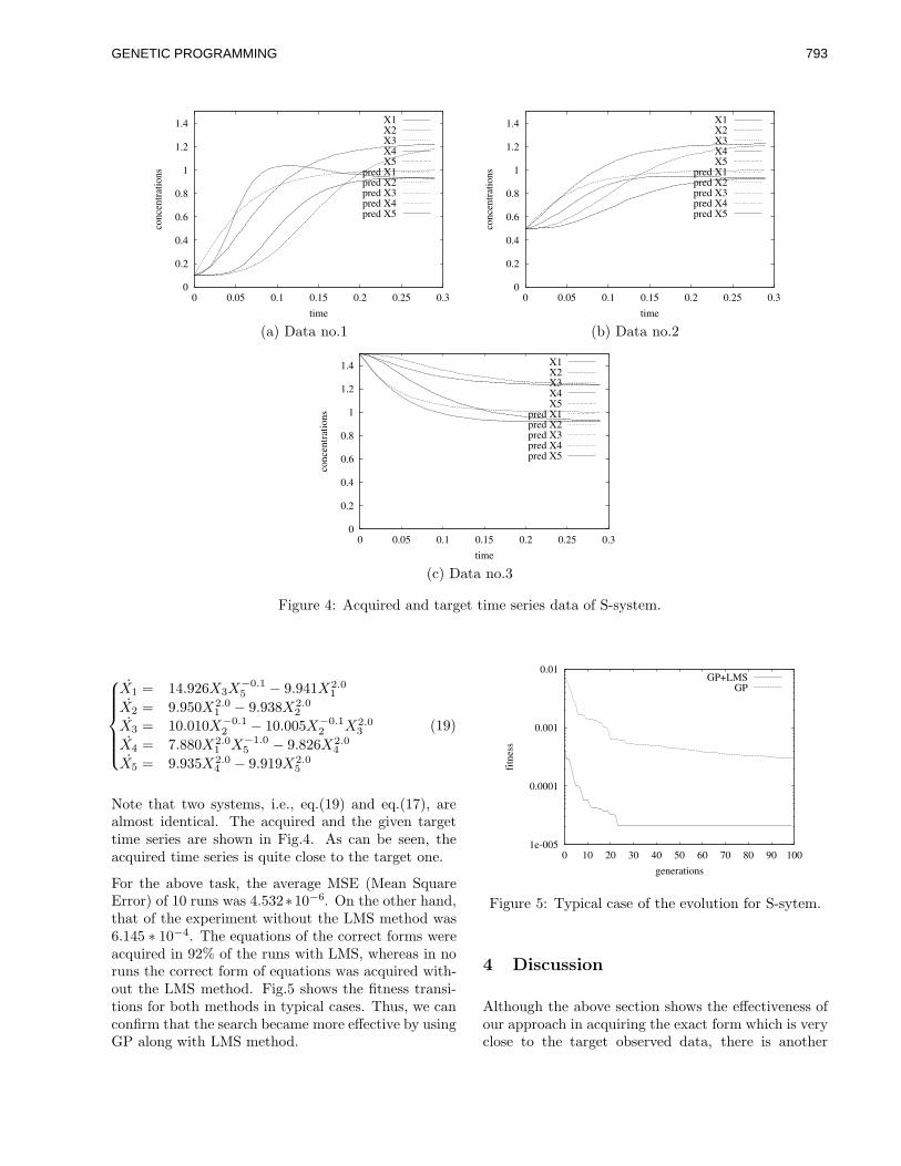
0

0.2

0.4

0.6

0.8

1

1.2

1.4

0 0.05 0.1 0.15 0.2 0.25 0.3

conc

entr

atio

ns

time

X1X2X3X4X5

pred X1pred X2pred X3pred X4pred X5

0

0.2

0.4

0.6

0.8

1

1.2

1.4

0 0.05 0.1 0.15 0.2 0.25 0.3

conc

entr

atio

ns

time

X1X2X3X4X5


(a) Data no.1 (b) Data no.2

0

0.2

0.4

0.6

0.8

1

1.2

1.4

0 0.05 0.1 0.15 0.2 0.25 0.3

conc

entr

atio

ns

time

X1X2X3X4X5


(c) Data no.3

Figure 4: Acquired and target time series data of S-system.

X1 = 14.926X3X−0.15 − 9.941X2.0

1

X2 = 9.950X2.01 − 9.938X2.0

2

X3 = 10.010X−0.12 − 10.005X−0.1

2 X2.03

X4 = 7.880X2.01 X−1.0

5 − 9.826X2.04

X5 = 9.935X2.04 − 9.919X2.0

5

(19)

Note that two systems, i.e., eq.(19) and eq.(17), arealmost identical. The acquired and the given targettime series are shown in Fig.4. As can be seen, theacquired time series is quite close to the target one.

For the above task, the average MSE (Mean SquareError) of 10 runs was 4.532∗10−6. On the other hand,that of the experiment without the LMS method was6.145 ∗ 10−4. The equations of the correct forms wereacquired in 92% of the runs with LMS, whereas in noruns the correct form of equations was acquired with-out the LMS method. Fig.5 shows the fitness transi-tions for both methods in typical cases. Thus, we canconfirm that the search became more effective by usingGP along with LMS method.

1e-005

0.0001

0.001

0.01

0 10 20 30 40 50 60 70 80 90 100

fitn

ess

generations

GP+LMSGP

Figure 5: Typical case of the evolution for S-sytem.

4 Discussion

Although the above section shows the effectiveness ofour approach in acquiring the exact form which is veryclose to the target observed data, there is another


factor to be considered, i.e., the robustness. To testthe robustness of our method to the real noisy world,we conducted the E-cell experiment (i.e., Exp.2) withnoise-added data sets. 5% and 10% random noiseswere added to the target time series. The acquiredtime series are plotted in Fig.6 with the target data.The MSE values and the success ratios averaged over15 runs are shown in Table 3. The table comparesthese values by our approach and the standard GP,in which the right hand sides of ODEs are evolved ina similar way to the symbolic regression (see [Koza92]for details). We can observe that the proposed methodworked effectively to acquire the better individual withnoisy environments than the standard GP.

0

0.5

1

1.5

2

2.5

0 0.05 0.1 0.15 0.2 0.25 0.3 0.35 0.4

conc

entr

atio

n

time

X1X2X3


(a) Standard GP.

0

0.5

1

1.5

2

2.5

0 0.05 0.1 0.15 0.2 0.25 0.3 0.35 0.4

conc

entr

atio

n

time

X1X2X3


(b) Proposed method.

Figure 6: Acquired time series of noisy data.

As can be seen in Section3.1, the proposed approachis superior to the traditional method [Cao00]. Re-member that the coefficients of ODEs were derivedby means of GA in Cao’s scheme, whereas we usedLMS for this purpose. Therefore, the superiority ofour approach can also be confirmed when we considerthe difference of computational burden of these tech-

niques.

As with many other proposed models, the solutionwhich fits the given time series quite well is not nec-essarily determined uniquely. In other words, theremay exist more than one solution which behave consis-tently with the target. Therefore, even if one systemof ODEs is acquired as a solution, we cannot disre-gard other candidates. Our aim is to obtain the candi-dates scattered in the huge search space and to proposeto users the possible causal relationship among theobservable components. Therefore, as future works,we will concentrate on the construction of the inter-active system, which proposes the possible solutionsand tells users what kinds of data are needed to de-termine the relationship among the components (see[Mimura and Iba02] for details).

5 Conclusion

We have proposed the inference method of the systemof ODEs from the observed time series by using GPalong with the LMS method. We showed how success-fully our method can infer the causal model by severalexperiments. More precisely, we succeeded in acquir-ing the system of ODEs which is very close to theobserved time series and inferring the exact equationform. The effectiveness of the LMS method and thesuperiority of our approach over the previous methodwere confirmed by comparative experiments.

As a future research, we will apply our approach tosome real-world tasks. For this purpose, we are work-ing on the development of the interactive inference sys-tem, in which users will be able to pick up the cor-rect equations or discard the meaningless equationsfrom the suggested ones. We are trying to solve someof the real biological problems by using this system[Mimura and Iba02].

References

[Babovic00] Babovic, V., and Keijzer, M., Evolu-tionary algorithms approach to induction ofdifferential equations, in Proc. of Geneticand Evolutionary Computation Conference(GECCO2000), pp.251-258, 2000.

[Cao00] Cao, H., Kang, L., Chen, Y., Yu, J., Evolu-tionary Modeling of Systems of Ordinary Dif-ferential Equations with Genetic Program-ming, Genetic Programming and EvolvableMachines, vol.1, pp.309-337, 2000.

[Iba94] Iba, H., deGaris, H., Sato, T., GeneticProgramming using a Minimum Descrip-


Noise 0% 5% 10%MSE Success ratio MSE Success ratio MSE Success ratio

Our method 2.54−03 100% 2.83−03 100% 8.04−03 67%Standard GP 1.25−02 40% 1.44−02 33% 1.52−02 33%

Table 3: The comparison of two methods in noisy environments.

tion Principle, in Advances in Genetic Pro-gramming, Kinnear,K.Jr. (ed.), MIT Press,pp.265-284, 1994.

[Koza92] Koza,J., Genetic Programming, MIT Press,1992.

[Mimura and Iba02] Mimura,A. and Iba,H., Inferenceof a Gene Regulatory Network by Meansof Interactive Evolutionary Computing, inProc. of Fourth Conference on Compu-tational Biology and Genome Informatics,(CBGI-02), 2002.

[Nikolaev and Iba01] Nikolaev,N. and Iba,H., Regu-larization Approach to Inductive GeneticProgramming, IEEE Transaction on Evolu-tionary Computation, vol.5, no.4, 2001.

[Sakamoto and Iba00] Sakamoto, E., Iba, H., Identify-ing Gene Regulatory Network as DifferentialEquation by Genetic Programming, in Proc.of 11th Genome Informatics Workshop, Uni-versity Academy Press, 2000.

[Sakamoto and Iba01] Sakamoto, E., Iba, H., Infer-ring a System of Differential Equations for aGene Regulatory Network by using GeneticProgramming, in Proc. of the 2001 Congresson Evolutionary Computation (CEC2001),2001.

[Savageau76] Savageau, M.A., Biochemical Systemsanalysis: a study of function and design inmolecular biology, Addison-Wesley, Reading,1976.

by Y Takeuchi

[Takeuchi96] Takeuchi, Y., Global Dynamical Proper-ties of Lotka-Volterra Systems ,World Scien-tific, 1996.

[Tominaga00] Tominaga, D., Koga, N., Okamoto, M.,Efficient Numerical Optimization AlgorithmBasedon Genetic Algorithm for Inverse Problem,Proc. of Genetic and Evolutionary Computa-tion Conference (GECCO2000), pp.251-258,2000.

[Tomita99] Tomita,M., Hashimoto,K., Takahashi,K.,Shimizu,T.S., Matsuzaki,Y., Miyoshi,F.,Saito,K., Tanida,S., Yugi,K., Venter,J.C.,and Hutchison,C.A.,3rd, E-CELL: softwareenvironment for whole-cell simulation, Bioin-formatics, vol.15,no.1, pp.72-84, 1999.

[Zhang95] Zhang, B.-T. and Muehlenbein, H., Balanc-ing accuracy and parsimony in genetic pro-gramming, Evolutionary Computation, vol.3,no.1, pp.17–38, 1995.


ABSTENTION REDUCES ERRORS DECISION ABSTAINING N-VERSION GENETIC PROGRAMMING

Abstract

Optimal fault masking N-Version Genetic Programming (NVGP) is a technique for building fault tolerant software via ensemble of automatically generated modules in such a way as to maximize their collective fault masking ability. Decision Abstaining N-Version Genetic Programming is NVGP that abstains from decision-making, when there is no decisive vote among the modules to make a decision. A special course of action may be taken for an abstained instance. We found that decision abstention contributed to error reduction in our experimental Escherichia coli DNA promoter sequence classification problem. Though decision abstention may reduce errors, high abstention rate makes the system of little use. This paper investigates the trade-off between abstention rate and error reduction.

1 INTRODUCTION

This paper investigates the effect of an abstention threshold on the trade-off between abstention rate and error reduction, using an N-Version Genetic Programming ensemble classifier [1].

An ensemble binary classifier makes a yes/no decision based on votes from the participating ensemble member classifiers. A decision abstention occurs, when there is no decisive vote among the ensemble modules to make decision. An unanimous vote is the most decisive (highest ensemble confidence), while a tie vote is the least decisive (lowest ensemble confidence). The abstention threshold is set somewhere between these two extremes. If the vote count of either “yes” or “no” does not reach to this threshold, the ensemble abstains from decision-making. The ensemble, thus, produces three outputs: yes, no, and don’t know. A special course of action may be taken for an abstained instance (such as classification by human experts) [2]. Abstention reduces the number of errors,

potentially avoiding overfitting [2]. However, if the ensemble classifier abstains too often, it is of little use. Our experimental test problem is Escherichia coli DNA promoter sequence classification. This problem has been explored with artificial neural networks [3][4][5] and genetic programming [6].

1.1 BRIEF INTRODUCTION OF N-VERSION GENETIC PROGRAMMING (NVGP)

N-Version Genetic Programming (NVGP), which provides an optimal fault masking ensemble of automatically generated modules, is a new technique for building fault tolerant software that significantly reduces errors when applied to an E. coli promoter sequence classification problem [1]. Genetic programming is used to provide a large pool of candidate modules with sufficient diversity to allow us to select an ensemble whose faults are nearly uncorrelated. We find ensembles with a high degree of fault masking by randomly sampling from this large pool of modules. The ensembles that produce the expected error rate are retained. The expected failure rate f for n independent components, each of which fails with probability p, where the composite system requires m component faults in order to fail (initially derived for n-modular redundant hardware systems [7]) is

For an N-version classifier system, such as ours, the i-th individual fault rate pi is the ratio of misclassified examples to the total number of training instances. In this case, f is the failure rate of an ideal ensemble. If the fault rate is the same for every pi, f is an area under a binomial probability density function as shown in the above formula. The failure rate of an ensemble is close to the theoretically optimal rate f precisely when component failures are not correlated. This is our criterion for selecting the qualified ensembles. Explicit quantification of the module diversity with the theoretical failure probability is a distinct feature of NVGP, guaranteeing phenotypic diversity and the optimal ensemble.

Kosuke Imamura Robert B. Heckendorn Terence Soule James A. Foster

Initiative for Bioinformatics and Evolutionary STudies (IBEST), Dept. of Computer Science,

University of Idaho, Moscow, ID 83844-1010 {kosuke,heckendo,tsoule,foster}@cs.uidaho.edu

. ( )kknn

mkpp

k

nf −

=−

= ∑ )1(


N-version programming (NVP) was an early approach to building fault tolerant software that adapted proven hardware approaches to fault tolerance [8]. A fundamental assumption of the NVP approach was that independent programming efforts would reduce the probability that similar errors will occur in two or more versions [9]. But this assumption was questioned, because experiments showed that modules developed for NVP tended to fail under similar circumstances. For example, Knight and Leveson rejected the hypothesis of the assumed independence of faults by independently developed programs [10]. However, this conclusion does not invalidate NVP in general. Hatton showed that his 3-version NVP system increased the reliability by a factor of 45. Though this is far less than the theoretical improvement of a factor of 833.6, it is still a significant improvement in system reliability [11].

The next section reviews previous work on abstention and ensemble methods.

2 PREVIOUS WORK Different ensemble construction methods have been studied in an effort to enhance accuracy. This section reviews abstention, averaging, median selection, boosting, and bagging. All methods exploit heterogeneity of ensemble components in one way or another.

2.1 ABSTENTION

Freund, et al., showed the error bound of averaging classifier with abstention [2]. The abstention threshold is based on the log ratio of the weighted sum of positive predictions and negative predictions. If the absolute value of this log ratio is smaller than the threshold, the ensemble classifier abstains from predicting. They identify the region of abstention as the locations of potential overfitting. Their theoretical work shows that the error of such predictor cannot be worse than twice of the best individual.

2.2 AVERAGE AND MEDIAN

A simple averaging method gathers outputs from all component modules and calculates their arithmetic average. Imamura and Foster showed simple averaging reduces error margins in path prediction [12] and function approximation with evolved digital circuits [13]. Another approach is weighted averaging, in which component modules are assigned optimal weights for computing a weighted average of the module outputs. Linearly optimal combination of artificial neural networks takes this approach [14][15]. Zang and Joung proposed Mixing Genetic Programs (MGP). MGP chooses a pool of individuals from a population and the master unit assigns the voting weights to these individuals using an additive weighting scheme [16]. The median value of the outputs is then the ensemble output. Soule approximated the sine function by taking the median of individuals, which were evolved, with subset of the entire training set for specialization [17]. Brameier and Banzhaf evolved teams

of predictors. The individuals are coevolved as a team as opposed to post-evolutionary combination [18].

2.3 BOOSTING AND BAGGING

Boosting and bagging are methods that perturb the training data by resampling to induce classifier diversity. The AdaBoost algorithm trains a weak learner (slightly better than random guessing) by iterating training while increasing the weights of misclassified samples and decreasing the weights of correctly classified ones [19]. The effect is that the weak learner focuses more and more on the misclassified samples. The trained classifiers in each successive round are weighted according to their performance. The final decision is a weighted majority vote. Bagging (Bootstrap aggregating) replicates training subsets by sampling with replacement [20]. It then trains classifiers separately on these subsets and builds an ensemble by aggregating these individual classifiers. For evolutionary computation, Iba applied Boosting and Bagging to genetic programming and his experiment validated their effectiveness and their potential for controlling bloat [21]. Land used a boosting technique to improve performance of Evolutionary Programming derived neural network architectures in a breast cancer diagnostic application [22]. However, both techniques have limitations. Boosting is susceptible to noise, Bagging is not any better than a simple ensemble in some cases, neither Boosting nor Bagging is appropriate for data poor cases, and bootstrap methods can have a large bias [19, 23, 24, 25, 26, 27].

2.4 CLASSIFICATION OF ENSEMBLES

Table 1 categorizes current ensemble methods in genetic programming in terms of their sampling technique in combination with the evolutionary approach. In cooperative methods [17][28], speciation pressure (such as that caused by crowding penalties [28]) plays a vital role in evolving heterogeneous individuals, while in isolation methods there is no interaction between individuals during evolution. Resampling methods create different classifiers by using different training sets (bagging) or varying weights of training instances (boosting). Non-resampling methods create different classifiers from the same training set with or without explicit speciation pressure. NVGP and Decision abstaining NVGP are non-resampling techniques based on isolated evolution of diverse individuals.

Table 1. Classification of ensemble creation methods.

Evolutionary Training set selection

Approach Resampling Non-resampling

Non-Isolation Boosting Crowding

Isolation Bagging NVGP


3 EXPERIMENT This section briefly summarizes the NVGP computational method (for detail description, see [1]) and presents the test results. We first run NVGP then incorporate abstention threshold to it. Our experimental problem is to classify whether a given DNA sequence is an E. coli promoter, using a decision abstaining NVGP. The data set is taken from UCI ML repository [29]. It contains 53 E. coli DNA promoter sequences and 53 non-promoter sequences of length 68.

3.1 COMPUTING ENVIRONMENT

The cluster supercomputing facilities from the Initiative for Bioinformatics and Evolutionary STudies (IBEST) is used to implement distributed computation. This device uses commodity computing parts to build substantial computing power for considerably less money than traditional supercomputers1. (http: //www.cs.uidaho.edu/ thecollective). This machine enabled experiments that would normally run for a month to complete in half a day.

3.2 INPUT AND OUTPUT

We used 2-gram encoding for input [30]. The 2-gram encoding counts the occurrences of two consecutive input characters (nucleotides) in a sliding window. Since there are four characters in DNA sequences (“a”, “c”, “g”, “t”), we have 16 unique two-character strings to count. For example, a sequence “caaag” will be encoded as {ca=1, aa=2, ag=1}. The classifier clusters the positive instances and places the negative instances outside the cluster. The cluster is defined by the mean output value of postitve instances ± 3*(standard deviation). If an output value from a given sequence falls in the cluster, it is classified as a promoter. Otherwise, it is classified as a non-promoter.

3.3 CLASSIFIER

3.3.1 Target Machine Architecture

Our classifier is a linear genome machine [31], which mimics MIPS architecture [32]. There are two instruction formats in this architecture: (Opcode r1,r2,r3) and (Opcode r1,r2,data). The instructions are ADDI, ADDR, MUL, DIV, MULI, DIVI, SIN, COS, LOG, EXP, NOP, MOVE, LOAD, CJMP, and CJMPI. The length of an individual program is restricted to a maximum of 80 instructions. Each evolving individual (a potential component for our NVGP ensemble system) used sixteen read-only registers for input data, which contained counts for individual nucleotide 2-grams as described above, and four read/write working registers.

1 The total cost of the machine is about US$44,000. Micron Technology generously donated all of the memory for the machine.

3.3.2 Genetic Programming

We used 5 crossover methods. Methods (1) and (2) are traditional one and two point crossover, respectively. Method (3) is one point crossover with inversion applied to each crossover segment. Methods (4) and (5) use four random crossover points, with (5) being a single parent recombination operator. Fitness is calculated by the following correlation formula

where P and N are numbers of correctly identified positives and negatives, and Pf and Nf are the numbers of falsely identified positives and negatives [33]. Steady state is used for population replacement. Evolution continues until an individual of fitness 0.8 or above appears.

3.3.3 Evolution and Ensemble Testing

A common holdout test divides the dataset into 2 exclusive sets, 2/3 for the training set and 1/3 for the test set [27]. Our training sets used a random sample of 35 (53*2/3) positive and 35 negative examples, and used the remaining examples for the test sets. We performed experiments for 10 different holdout sets. The evolution and ensemble procedures are described below:

1. Create a training set and test set.

2. Evolve 40 isolated islands with 100 individuals each in parallel. Add an individual whose fitness is 0.8 from each island to a set B of single best versions.

3. Select N individuals by uniform-random sampling from B for N=15, 31 to form an NVGP ensemble. See 3.4.1 for the sampling frequency.

4. Evaluate the performance of each ensemble. If the ensemble is qualified, then retain it for a test set trial. Goto 3. The ensemble is qualified if the difference between the number of errors expected when versions have independent faults and the number of errors observed is small (less than one in our case).

3.4 EXPERIMENTAL RESULTS

The evolution and ensemble testing procedure described in section 3.3 is repeated for 10 different holdout tests in an attempt to reduce stochastic errors caused by sampling in performance estimation. We first show the performance of NVGP without abstention, then with abstention. We assume the number of errors have a normal distribution, since each test instance can be viewed as a Bernoulli trial [27].

3.4.1 Performance of NVGP

There are 40×109 and 27×107 possible ensembles to be formed respectively for 15 and 31 voter systems out of 40 candidate modules. Uniform random search sampled approximately 40×103 and 27×103 ensembles for 15 and 31 voter ensembles respectively, from which we selected

))()()(( ffff

ff

PPNPPNNN

NPPNC

++++

−=


qualified ensembles for statistics. Table 2 shows the numbers of qualified ensembles found for each test. For example, we found 23199 qualified 15-voter ensembles out of 40×103 samples for the test 1. Table 3 is the result of t-test on the null hypothesis that average performance of the ensembles and the single best versions is not significantly different. Table 4 is the result of F-test on the null hypothesis that standard error of the ensembles and the single best versions is not significantly different. Table 5 shows error reduction percentage observed in ensembles relative to the error rates of the single best versions in the set B (see 3.3.3). It represents the average error reduction

achieved by NVGP over single modules produced by genetic programming.

Figure 1 presents the performance distribution intervals of the single best versions and the corresponding N-voter NVGP ensemble at a 90% limit. For each holdout test, we present statistics for the single best versions, and for each of the four NVGP ensembles (N=15, 31). For example, the leftmost bar in holdout test 1 is the performance distribution of the 40 single best versions, showing that the best is estimated to be 20% error and the worst to be 48%, with a mean of 34%. The middle bar is 15-voter and the rightmost bar is 31-voter ensembles.

Table 2. The number of sampled qualified-ensembles

test1 test2 test3 test4 test5 test6 test7 test8 test9 test10

15-voter 23199 29370 11596 8601 15973 4267 30455 32141 13171 17279

31-voter 19650 27205 9910 3197 13778 814 27340 27340 7672 23113

Table 3. The result of t-test, degree of freedom .≅ 40 for all the test cases.


15-voter 11.07 9.10 3.27 8.67 9.67 10.21 8.80 6.06 6.64 5.46

31-voter 14.08 10.47 2.14 8.17 10.54 13.53 9.30 5.78 6.62 6.94

Table 4. The result of F test on error rate standard deviations


15voter 3.15 4.10 4.98 3.53 4.01 2.22 2.71 4.37 7.22 3.76

31-voter 7.17 6.47 12.03 9.36 10.89 4.71 8.13 24.11 47.44 8.07

Table 5. Percentage error reduction of NVGP relative to set of best individual in isolation


15-voter 44 33 14 31 40 31 37 22 25 24

31-voter 56 38 9 29 43 42 39 21 25 31

Figure 1. Error rate distribution intervals of the single best versions and the corresponding N-voter NVGP ensemble at a 90% limit. Leftmost, middle, and rightmost bars are distribution ofsingle-version, 15-voter, and 31 voter system respectively.


0

0.1

0.2

0.3

0.4

0.5

0.6


3.4.2 Behavior of Decision Abstaining NVGP

The abstention thresholds are incorporated into the NVGP outputs of 3.4.1. The decision abstaining ensemble requires abstention threshold, h, and needs ((N+1)/2 + h) votes, either positive or negative, to make a decision, where N (odd) is the number of vote participating individuals. The voting scheme is a simple majority rule, if h=0. Figure 2 and 3 are the plots of the abstention rates and the error rates of 15 and 31 voter ensemble for the 10 holdout tests with respect to the abstention threshold, h. Figure 4 represents the average abstention and error rates from figure 2 and 3 for collective analysis. The error rate is a decreasing function and the abstention rate is an increasing function.

4 DISCUSSION

4.1 NVGP

Though a holdout test is commonly used to measure performance of evolutionary algorithms, it is not reliable. Kohavi argues that holdout testing does not provide a good estimate of error rate [27]. Nonetheless, we repeated the holdout test 10 times with different training/test sets for somewhat fair statistics. In figure 1, the hold-out test 3 does not exhibit apparent superiority of NVGP as in the test 1, though we reject the null hypothesis that average performance of single best version and NVGP are not significantly different at α=0.975. For all the other nine test cases, we reject the hypothesis virtually at 100% and conclude that NVGP is superior. NVGP error rates in all ten tests are far below the theoretical bound shown by

Freund [2] even without abstention. Table 4 indicates that performance fluctuation of NVGP is statistically significantly smaller than single versions. Apparently, as the ensemble size approaches to the pool size, the performance fluctuation becomes smaller. If we combine all the individuals in the pool, there is no performance fluctuation. Therefore, a larger fluctuation may be expected for NVGP if the component pool size is huge. But, also true is that duplicate phenotypes start populating the pool as the pool size becomes larger. In fact, our experiment witnessed that an exhaustive search for an optimal ensemble of 39 voters from the pool failed in three out of the ten holdout tests. This possibly indicates that the entropy of the pool may have reached a plateau with the given training data and training method. If this is the case, the small performance fluctuation for optimally sized NVGP will still hold regardless of the pool size increase. Further study is needed for an optimal size of NVGP.

Notice that a single best individual has a chance to become practically a random classifier (error rate above 0.4) roughly 10%-20% of the time on unseen data. Unfortunately, we have no way of knowing which individual would become a random classifier beforehand, because they all have the same fitness (0.8) on the training set. This is the risk we must bear with a single best classifier. Fluctuation in performance is the very reason why we compared the distributions, and why NVGP has superior performance.

4.2 ABSTENTION

Figure 4 shows (see dashed lines) that the decision abstaining NVGP achieved a near zero error rate, at high

0.0

0.2

0.4

0.6

0.8

1.0

1 2 3 4 5 6 7 abstention threshold

0.0

0.2

0.4

0.6

0.8

1.0

1 3 5 7 9 11 13 15 abstention threshold

erro

r/ab

sten

tion

Figure 2. abstention rate and error rate for 15 voter system

Figure 3. abstention rate and error rate for 31 voter system

0.0

0.2

0.4

0.6

0.8

1.0

1 3 5 7 9 11 13 15

abstention rate

error rate

0.0

0.2

0.4

0.6

0.8

1.0

1 2 3 4 5 6 7

Figure 4. average abstention and error rates from figure 2 and 3.

error rate

abstention


cost of abstention rate, approximately 80%, for both 15-voter and 31-voter ensembles. Abstention rates 29% of 15-voter and 28% of 31-voter ensembles give 50% error reduction over NVGP alone (no abstention). Whether these abstention rates are acceptable for error reduction depends on how critical it is to have wrong predictions.

The abstention rates and the error rates are monotonic with respect to the abstention thresholds, and the trade-off between abstention and error reduction can be estimated almost linearly. Consequently, there is no analytically measurable peak gain by abstention. Subjective judgment must be used to set the abstention threshold. The following formula may be used to numerically measure the effect of abstention: Q= Ea + ρN, where Ea is the number of errors with abstention, N is the number of don’t know outputs, and 0�ρ�� ,I ρ=1, then don’t know is as bad as wrong prediction and counted as an error. On the other extreme, if ρ=0, it is as good as correct prediction. The larger the ρ value is the more penalties for don’t know outputs.

Let the number of errors of NVGP alone (no abstention) be Ez. If Q � (z, then we are unconditionally better off with abstention. For example, setting ρ=0.5 (half way between correct and incorrect prediction), we obtain Q values for 31-voter ensembles as shown in Table 6. The Q values are fairly close to Ez when the threshold is 1, which gives 3.2% error reduction (Figure 4 data). In other words, threshold = 1 is a break-even point for the trade-off between abstention and error reduction for ρ=0.5. For safety critical applications, such as medical diagnostics, a smaller ρ value would be appropriate for the trade-off analysis. That is to say, do not penalize heavily when an ensemble is trying to avoid a random guess. It may well be the case where the training set was inappropriate for particular instances.

4.3 POST-EVOLUTIONARY COMBINATION

Post-evolutionary combination is thought to be computationally inefficient, because many runs are required to obtain a sufficient number of individuals [18]. However, inexpensive cluster computing alleviates this problem (see section 3.1). Not only can the post-evolutionary search for the optimal NVGP ensemble be performed in parallel, but also the search may no longer need to be continued after an optimal ensemble is found.

5 CONCLUSION AND FUTURE RESEARCH

We showed the experimental classification result by NVGP, which significantly improved accuracy and reduced the performance fluctuation. Then, we incorporated decision abstention to it. Abstention in effect avoids random guesses when the ensemble confidence is low, i.e., votes are too close to call. It is a viable method to reduce errors. The trade-off between abstention and error reduction is subjective. The abstention threshold value depends on how critical an application is.

It is important to curve the abstention rate increase. We plan to embed the individual confidence to enhance the ensemble confidence. The individual confidence, in our case, can be measured by the distance of an instance from the cluster center. The further the distance, the lower the confidence. The ensemble confidence in prediction is measured by the level of disagreement among the voters.

Acknowledgments

This work is supported by the Initiative for Bioinformatics and Evolutionary STudies (IBEST) at the University of Idaho; by NIH NCRR grant 1P20RR016454-01; and by NIH NCRR grant NIH NCRR 1P20RR016448-01; and by NSF grant NSF EPS 809935. We are grateful to colleagues in the Initiative for Bioinformatics and Evolutionary STudies (IBEST) for insightful discussions. Finally, we wish to thank the many students who designed and built our Beowulf cluster, and Micron Technology for donating the memory for that machine. We thank John Cavalieri and Janet Holmberg for proofreading.

References

1. Imamura, K., Heckendorn,R B., Soule, T., Foster, J A.: N-version Genetic Programming via Fault Masking Proceedings of the Euro EuroGP2002 5th European Conference on Genetic Programming (To appear)

2. Freund, Y., Mansour, Y., Schapire, R E.: Why Averaging Classifiers Can Protect Against Overfitting. Proceedings of the 8th International Workshop on Artificial Intelligence and Statistics,2001 (www.ai.mit.edu/confereces/aistats2001/papers.html)

Table 6. Q values for 31-voter ensembles (ρ=0.5)

abstention threshold test1 test2 test3 test4 test5 test6 test7 test8 test9 test10

0 6.7 8.0 10.1 7.7 6.8 8.8 7.3 10.4 9.1 9.5

1 7.2 8.3 10.0 7.9 7.1 9.1 7.6 10.6 9.0 9.7

2 8.5 9.2 9.8 8.4 7.8 9.9 8.6 11.1 9.1 10.2

3 10.5 10.5 10.1 9.5 9.3 11.2 10.1 12.2 9.8 11.0


3. Pedersen, A.G., Engelbrecht, J.: Investigations of Escherichia Coli promoter sequences with artificial neural networks: New signals discovered upstream of the transcriptional startpoint. Proceedings of the Third International Conference on Intelligent Systems for Molecular Biology (1995) 292-299 (http://citeseer.nj.nec.com/25393.html)

4. Towell,G.G., Shavlik, J.W., Noordewier, M.O.: Refinement of approximate domain theories by knowledge-based neural networks. Proceedings of AAAI-90 (1990) 861-866 (http://citeseer.nj.nec.com/towell90refinement.html)

5. Ma, Q., Wang, J.T.L.: Recognizing Promoters in DNA Using Bayesian Neural Networks. Proceedings of the IASTED International Conference, Artificial Intelligence and Soft Computing (1999) 301-305 (http://citeseer.nj.nec.com/174424.html)

6. Handley, S.: Predicting Whether Or Not a Nucleic Acid Sequence is an E. Coli Promoter Region Using Genetic Programming. Proceedings of First International Symposium on Intelligence in Neural and Biological Systems, IEEE Computer Society Press, (1995) 122-127

7. Pradhan, D. K., Banerjee, P.: Fault-Tolerance Multiprocessor and Distributed Systems: Principles. In Pradhan, D.K.: Fault-Tolerant Computer System Design. Chapter 3, Prentice Hall PTR, (1996), 142

8. Avizienis, A. and J.P.J. Kelly: Fault Tolerance by Design Diversity: Concepts and Experiments. IEEE Computer, vol. 17 no. 8, (1984), 67-80

9. Victoria Hilford., Lyu, M. R., Cukic B., Jamoussi A., Bastani F. B.: Diversity in the Software Development Process. Proceedings of Third International Workshop on Object-Oriented Real-Time Dependable Systems, IEEE Comput. Soc, (1997), 129-36 (http://www.cse.cuhk.edu.hk/~lyu/papers.html#SFT_Techniques)

10. Knight, J.C., Leveson, N.B.: An Experimental Evaluation of the Assumption of Independence in Multiversion Programming. IEEE Transaction on Software Engineering, vol. SE-12, no. 1 (1986)

11. Hatton, L.: N-version vs. one good program. IEEE Software, vol 14, no. 6 (1997) 71-76

12. Imamura, K., Foster, J.A.: Fault Tolerant Computing with N-Version Genetic Programming. Proceedings of Genetic and Evolvable Computing Conference (GECCO), Morgan Kaufmann, (2001) 178

13. Imamura, K., Foster, J.A.: Fault Tolerant Evolvable Hardware Through N-Version Genetic Programming. Proceedings of World Multiconference on Systemics, Cybernetics, and Informatics (SCI), vol. 3, (2001) 182-186

14. Hashem, S.: Optimal Linear Combinations of Neural Networks. Neural Networks, vol. 10, no. 4, (1997) 599-614

(http://www.emsl.pnl.gov:2080/proj/neuron/papers/hashem.nn97.abs.html)

15. Hashem, S.: Improving Model Accuracy Using Optimal Linear Combinations of Trained Neural Networks. IEEE Transactions on Neural Networks, vol.6, no.3 (1995) 792-794 (www.emsl.pnl.gov :2080/proj/neuron//papers/hashem.tonn95.abs.html)

16. Zang, B-T., Joung, J-G.: Enhancing Robustness of Genetic Programming at the Species Level. Proceedings of the 2nd Annual Conference Genetic Programming 97, Morgan Kaufmann (1997) 336-342.

17. Terence Soule, “Heterogeneity and Specialization in Evolving Teams”, Proceeding of Genetic and Evolvable Computing Conference (GECCO), Morgan Kaufmann (2000) 778-785

18. Brameier, M., Banzhaf, W.:Evolving Teams of Predictors with Linear Genetic Programming. Genetic Programmin and Evolvable Machines, vol. 2, (2001) 381-407

19. Schapire R.E., Freund, F.: A Short Introduction to Boosting. Journal of Japanese Society for Artificial Intelligence 14, no. 5, (1999) 771-80 (http://citeseer.nj.nec.com/freund99short.html)

20. Breiman, L.: Bagging Predictor. Technical Report No.421, Department of Statistics, University of California Berkley, 1994 (http://www.salford-systems.com/docs/BAGGING_PREDICTORS.PDF)

21. Iba, H.: Bagging, Boosting, and Bloating in Genetic Programming. Proceedings of the Genetic and Evolutionary Computation Conference, vol. 2, Morgan Kaufmann, (1999) 1053-1060

22. Land, W.H. Jr., Masters T., Lo J.Y., McKee, D.W., Anderson, F.R.: New results in breast cancer classification obtained from an evolutionary computation/adaptive boosting hybrid using mammogram and history data. Proceedings of the 2001 IEEE Mountain Workshop on Soft Computing in Industrial Applications. IEEE, (2001) 47-52

23. Basak, S.C., Gute, B.D., Grunwald, G.D., David W. Opitz, D.W., Balasubramanian, K.: Use of statistical and neural net methods in predicting toxicity of chemicals: A hierarchical QSAR approach. Predictive Toxicology of Chemicals: Experiences and Impact of AI Tools - Papers from the 1999 AAAI Symposium, AAAI Press, (1999) 108-111

24. Opitz, D.W., Basak, S.C., Gute, B.D.: Hazard Assessment Modeling: An Evolutionary Ensemble Approach. Proceedings of the Genetic and Evolutionary Computation Conference, vol. 2, Morgan Kaufmann (1999) 1643-1650

25. Maclin, R., Opitz, D.: An empirical evaluation of bagging and boosting. Proceedings of the Fourteenth International Conference on Artificial Intelligence, AAAI Press/MIT Press (1999) 546-551 (http://citeseer.nj.nec.com/maclin97empirical.html)


26. Bauer, E., Kohavi, R.: An Empirical Comparison of Voting Classification Algorithms: Bagging, Boosting, and Variants. Machine Learning, vol. 36, 1/2, Kluwer Academic Publishers (1999) 105-139 (http://citeseer.nj.nec.com/bauer98empirical.html)

27. Kohavi, R.: A Study of Cross-Validation and Bootstrap for Accuracy Estimation and Model Selection. Proceedings of the 14th International Joint Conference on Artificial Intelligence (IJCAI), Morgan Kaufmann (1995) 1137-1145 (http://citeseer.nj.nec.com/kohavi95study.html)

28. Soule, T.: Voting Teams: A Cooperative Approach to Non-Typical Problems. Proceedings of the Genetic and Evolutionary Computation Conference (GECCO-99), vol. 1,Morgan Kaufmann (1999) 916-922

29. UCI Machine Learning Repository, Molecular Biology Databases (http://www1.ics.uci.edu/~mlearn/MLSummary.html)

30. Wang, J.T.L., Ma, Q., Shash D., Wu, C.: Application of neural networks to biological data mining: a case study in protein sequence classification. Proceedings KDD-2000. Sixth ACM SIGKDD International Conference on Knowledge Discovery and Data Mining. ACM, (2000) 305-309 (http://citeseer.nj.nec.com/382372.html)

31. Banzhaf, W., Nordin, P., Keller, R.E., Francone, F.D.: Genetic Programming: An Introduction: On the Automatic Evolution of Computer Programs and Its Applications. Academic Press/Morgan Kaufmann (1998)

32. MIPS32™ Architecture for Programmers Volume I: Introduction to the MIPS32™ Architecture (http://www.mips.com/publications/index.html)

33. Matthwes, B. W.:Comparison of the predicted and observed secondary structure of T4 phage lysozyme. Biochimica et Biophysica Acta, vol. 405 (1975) 443-451


Collaborating with a Genetic Programming System to GenerateModular Robotic Code

Jeremy Kubica�

Carnegie Mellon University5000 Forbes AvenuePittsburgh, PA [email protected]

Eleanor Rie�el

FXPAL3400 Hillview Ave Bldg 4

Palo Alto CA 94304rie�[email protected](650) 813-7077

Abstract

While the choice of a set of primitives canstrongly e�ect the performance of geneticprogramming, the design of such a set re-mains more of an art than a science. Welook at a joint approach that combines bothhand-coding and genetic programming to de-�ne and re�ne primitives in the context ofa creating distribute control code for modu-lar robots. We give some rules of thumb fordesigning and re�ning sets of primitives, il-lustrating the rules with lessons we learnedin the course of solving several problems incontrol code for modular robots.

1 INTRODUCTION

It is well-known, from various \no free lunch" the-orems, that no single approach can e�ectively solveall problems (Wolpert, 1996; Wolpert and Mecready,1997). Thus it is necessary to tailor techniques to theproblem at hand. For genetic programming this tailor-ing can be done in three primary ways: choosing theprimitives, choosing the �tness functions, and choosingparameters for the algorithm such as the percentage ofuse of various operators. Here we look at the problemof e�ectively choosing primitives.

We describe techniques for and experiences with thejoint use of genetic programming and hand-coding todesign and re�ne sets of primitives for a variety of mod-ular robotics problems. The creation of decentralizedcontrol software for modular robots is a diÆcult prob-lem due to both the decentralized nature of the soft-ware and the fact that the connectivity relations be-tween the modules constantly change. Yet, in spite of

�* Supported by FXPAL

these diÆculties, or perhaps because of them, modularrobotics provides an ideal domain in which to exper-iment with automated software generation methods;there are many robotic tasks that are easily speci�edbut for which it is highly non-obvious what distributedsoftware would create the desired behavior.

Ideally, for the problem of robotic control, a set of

primitives could be derived directly from a descriptionof the hardware capabilities. While a description ofsuch capabilities is an excellent place to start, �nd-ing a solution given only the most basic actions canbe prohibitively time consuming. Another approach isto tailor the primitives to the task, which may requiresigni�cant development time. In fact, the developmenttime required for the primitives can approach that ofactually solving the problem. We take an intermediateapproach. Except for primitives that encode informa-tion speci�c to the problem (as opposed to its solu-tion), we try to provide primitives that would appearto be useful in a wide range of problems and are stillreasonably low-level. We use insights gained from bothhuman and machine attempts to solve the problems todesign e�ective sets of primitives.

2 MODULAR ROBOTIC

HARDWARE AND SIMULATOR

2.1 TELECUBE MODULES

Modular self-recon�gurable robots are systems consist-ing of a collection of simple and identical robotic mod-ules that can form connections to and move relativeto each other (Yim, 1994; Murata et. al., 1994; Rusand Vona, 2000). These modules function together toproduce an overall behavior of the robot, analogousto the way cells in a body function together. The factthat both the connectivity and relative positions of themodules can change allows the overall robot to recon-�gure and take on di�erent shapes. Modular robotic


Figure 1: One telecube module.

systems provide possible bene�ts in terms of exibility,adaptability, and robustness.

2.2 MODULE CAPABILITIES

2.2.1 Physical Capabilities

The robot modules we consider are the TeleCube mod-ules currently being developed at Xerox PARC andshown in Figure 1 (Suh et. al., 2002). They are sim-ilar in design to modules being designed and build atDartmouth (Rus and Vona, 2000), which can expandin two dimensions. The modules are cube shaped withan extendable arm on all six faces. The arms are as-sumed to extend independently up to half of the bodylength, giving the robot modules an overall 2:1 expan-sion ratio. For simplicity, we restrict the arms to fullyextended or fully retracted states. The expansion andcontraction of these arms provide the modules withtheir only form of motion. Latches on the plates atthe end of each arm allow two aligned modules to con-nect to each other. The arm motion together withthe latching and unlatching capability means that theconnectivity topology of a modular robot can changegreatly over time. As shown in (Vassilvitskii et. al.,2002), this motion is suÆcient to enable arbitrary re-con�guration within a large class of shapes.

2.2.2 Sensors, Communication, and Memory

Each module is assumed to have simple sensing andcommunication abilities that resemble those that willbe given to the TeleCube modules currently being builtat Xerox PARC. Modules can send limited bandwidthmessages to their immediate neighbors. Each mod-ule is also assumed to be able to sense contact at theend of each arm, sense how far each of their arms isextended, determine whether they are connected to aneighboring module, and detect nearby, adjacent mod-

ules. Each module has a small memory capacity, whichis initialized to all zeros. We also give the modules sim-ple computational abilities such as the capability to

determine the opposite of a given direction, the abilityto generate a random direction, and to calculate andstore the value of each of its position coordinates.

2.3 TELECUBE SIMULATOR

The experiments reported here were run by connectingFXPAL's genetic programming system to a simulator,written by J. Kubica and S. Vassilvitskii, for the Tele-Cube modular robots. The module control code isrepresented in a LISP-like parse tree that is evaluatedonce per time step for each module.

3 PROBLEM CONTEXTS

For all of the problems described here we are interestedin a completely decentralized solution in which the de-sired global behavior of the robot emerges from controlcode that is run locally on each of the modules thatmake up the robot. Decentralized control software isa challenging domain to begin with, and the fact thatthe connectivity relations between the modules con-stantly change makes modular robotic problems evenharder. The collaboration between hand-coding andautomatic generation of solutions is described belowin the context of three speci�c modular robotic con-trol problems to which we have applied this technique:the tunnel problem, the �ltering membrane problem,and the sorting membrane problem.

The tunnel problem consists of a long thin world, 40x 10 x 2 arm lengths, that is enclosed on all sides bywalls. During each of the trials an object is placedrandomly \in" one of the long walls. This means thata module adjacent to this location along the wall cansense the object, but will not be blocked by it or stuckbehind it while moving along the wall. The goal of themodules is to �nd the object and all move as close toit as possible. Thus, we de�ne our �tness function asthe sum of each module's distance to the object at theend of a run. The modules start out as a 3 x 3 x 1 gridcon�guration in one corner of the world.

The membrane problems consist of a membrane, athree-dimensional lattice of modules, and a foreignobject which, depending on its attributes, should orshould not be accepted into the membrane and ma-nipulated by it. In the case of a �ltering membrane,the object is either accepted or rejected. Accepted ob-jects are passed through the membrane and out thebottom, whereas rejected objects remain on top. Asorting membrane accepts all objects, but sorts them


along some axis. We looked at the case of a binarysorting membrane, which moves an object towards oneof two opposite ends depending on its value. For both

membrane problems we use �tness functions that mea-sure the distance of the object from where it oughtto end up and a penalty for the membrane breakingapart. Since the modules are unable to directly graspor pull the objects, all solutions to the membrane prob-

lem require the use of gravity, by having modules moveout from under the objects and allowing them to fallthrough the membrane. For more details on the mem-brane problems, including some pictures, see (Kubicaand Rie�el, 2002).

4 RELATED WORK

A number of researchers have looked at enabling a ge-netic programming system to add primitives on its ownin the course of its runs. Approaches include ADFs(Koza, 1994), libraries (Angeline and Pollack, 1994),subroutines (Rosca and Ballard, 1996), and subtreeencapsulation (Roberts et al., 2001). While such tech-niques might help with some of the problems we de-scribe here, we are particularly interested in how toadd primitives that the system would be unlikely to�nd for itself. Furthermore, there are many situa-tions, perhaps the majority, in which one is most in-terested in solving the problem at hand in any waypossible, rather than being concerned about the ex-tent to which the solution was automatically attained.We hope that what we write here can help others tohave more productive collaborations with a geneticprogramming system in order to more e�ectively solvepractical problems of interest.

The problem of automatic code generation for mod-ular robots has also seen interest recently. Kubicaet. al. (Kubica et. al., 2001) hand-coded controlprograms for internal object manipulation with robotsmade of TeleCube modules. Bennett et. al. (Bennettet. al., 2001) used genetic programming to generatedistributed control programs for modular robots con-sisting of sliding-style modules (Bennett and Rie�el,2000; Pamecha et al., 1996). It is important to notehowever that this sliding-style module design enablesmovement with primitive operations directly suggestedby the hardware. In particular, movement in that set-ting, unlike for the TeleCube modules, does not requireexplicit connection and disconnection actions. Thusmovement in their case avoids some of the diÆcultieswe faced when attempting to generate e�ective soft-ware for robots made from Telecube style modules.

5 DEVELOPING EFFECTIVE SETS

OF PRIMITIVES

5.1 BASIC PRIMITIVES

Each of the basic capabilities of the modules can becaptured by a primitive operation.

� Physical actions: (ExtendArm direction),(RetractArm direction), (Connect

direction), (Disconnect direction)

� Communication: (SendMessage direction type

value), (GetMessage direction type)

� Sensors: (HasNeighbor direction),(ReadSensorNeighborDist direction),(ReadSensorObjectDist direction)

� Memory: (ReadReg index), (SetReg index

value)

� Other: (OppDirdirection direction),(RandDir), and (GetX), (GetY), (GetZ).

In addition to these module speci�c primitive, we al-low the module control programs to use the followingbasic programming primitives: (Add), (Sub), (If),(ProgN) (LT), (And), and (Not), and the numericconstants 0.0, 0.1, 0.2, 0.4, 0.6, 0.8, and 1.0.

The primitives described above all mirror basic hard-ware capabilities of Telecube modules. For more de-tails on these primitives, see (Kubica and Rie�el,2002). However these primitives do not form an opti-mal set of primitives for either a human or a geneticprogramming system to construct e�ective software forthe tasks we described above. We look at how geneticprogramming experiments and hand-coding attemptstogether enabled the development of e�ective sets ofprimitives.

5.2 INITIAL CHOICE OF PRIMITIVES

Ask the system only to discover a solution, not aspects

of the problem

One important consideration when choosing primitivesis to give the system full information about the prob-lem. Even researchers more concerned with automati-cally generating code than solving problems per se andwho are resistent to giving the system any hints as tohow to solve the problem, should feel comfortable giv-ing the system enough information so that it does nothave to guess the problem as well as the solution.


0 5 10 15 20 25 30 35 40 45 5060

80

100

120

140

160

180

200

220

240

260

Generation

Ave

. Fitn

ess

With ReadSensorShouldPass Without ReadSensorShouldPass

Figure 2: Average solution performance on �lteringmembrane problem with and without ReadSensor-ShouldPass primitive.

In the �ltering membrane problem, the modules mustdetermine whether or not to accept an object. Inour case the criterion for the �lter to accept an ob-ject was that the value returned by (ReadObjectVal

direction) be above 0.5. In order to solve the prob-lem in our initial runs the GP system had to create asubtree testing for the acceptance criterion.

As we tried to gauge how the system was doing, werealized that we were using the existence of such asubtree to determine how close the GP system was toa solution. We soon realized that one should not re-quire an automatic code generation technique to guessthe problem as well as the solution, even if it can.Thus we added a primitive that encapsulates the �lter-ing criterion: the Boolean (ReadSensorShouldPass

direction) primitive

(LT(Add(0.4 0.1))(ReadObjectVal direction)).

Figure 2 shows the performance of two GP runs,one with the ReadSensorShouldPass primitive andone without it. While the system could solvethe problem without the (ReadSensorShouldPass

direction) primitive, its addition certainly helped.Further, for the evolution of the membrane controlthere is no reason to withhold this type of informa-tion about the problem statement itself. Note thatthis situation is di�erent from one in which one mightbe trying to learn a good criterion, say for identifyingdefective parts or a distinguishing characteristic of aset of objects.

Avoid large needle-in-the-haystack searches

The tasks we describe above all require movement, as

Figure 3: Module in white moves towards right.

do most modular robotic tasks including recon�gura-tion, locomotion, and internal manipulation. But noneof the �tness functions we used give any reward toprograms that have put together part, but not all, ofa sequence that would result in movement. Since noreward is given, the genetic programming system hasnothing to guide it towards movement.

Even at its simplest level, movement of a single Tele-Cube module is a complex process, involving bondingwith and unbonding from neighbors, expanding andcontract arms, and checking that the move is possible.To get an impression the complexity of a single move-ment, it is only necessary at look at the movementsubtree involved in disconnecting from the perpendic-ular neighbors:

(ProgN (ProgN (Disconnect 0.0) (RetractArm

0.0)) (ProgN (Disconnect 0.2) (RetractArm



0.6)))

The code above disconnects from the correct neigh-bors in the case the module is moving along the �Xaxis. Just to choose Disconnect and Retract armfrom just the four physical primitives has probablilityless than 10�3. Choosing the appropriate constants forthe Disconnect and Retract functions from the sevennumeric constants also has probability less than 10�5.And choosing the �ve ProbN primitives has probabil-ity less than 10�5. So the probability of �nding thecorrect components is less than 10�13.

Up to now we have only considered a subtree of thesort that would correctly disconnect a module. In ad-dition, one would need appropriate if statements todetermine the correct direction, the appropriate armexpansions and contractions to accomplish the move-ment, and a similar subtree to handle reconnectionwith any new neighbors. Thus, the simple move il-lustrated in Figure 3, given only the basic primitivesdescribed above, would require at least 12 di�erentprimitives and well over 50 nodes. More code wouldbe required to enable moves in all six directions, notjust one, and the graceful handling of movement fail-ures would require considerably more code. Thus thelikelihood that such a program would be created given


no guidance is impractically small.

With the basic primitives, and a simple �tness func-

tion with no gradient towards movement from none,the GP system would be searching blindly. Thus it isextrodinarily unlikely that the GP system would suc-ceed even in evolving movement. In fact the problemis harder still since only useful and used motion wouldbe rewarded. By asking genetic programming to evolve

movement, we are asking it to search for a needle, orrather a few needles, in a very large haystack.

A number of solutions are possible. One solutionwould be to change the �tness function so that it re-wards partial programs out of which movement couldbe constructed. Another possibility is to simply evolvemovement �rst and then use that solution as a prim-itive when evolving solutions to more complex tasks.Note that this approach still requires determining a�tness function that rewards partial solutions. It ishighly non-trivial to see how to design a principled re-ward system. Figuring out principled approaches tothis problem, and other similar problems, is an openresearch issue that ought to be of great interest to any-one trying to automatically solve problems. An un-principled way of solving this problem is to hand-codea solution and then reward programs based on simi-larity with this solution. One might as well use thehand-coded solution as a primitive in the �rst place,which is what we do.

Achieving simple motion, for instance the motion illus-trated in Figure 3, only requires reasoning at the locallevel and is thus easier for a human to do than solu-tions to tasks that require global behavior to emergefrom the local actions. Following basic operations usedby Kubica, et. al. (Kubica et. al., 2001), we createda movement primitive that enables modules to move adistance of one arm length in any of the six directions.The movement is accomplished by simultaneously con-tracting the front arm and expanding the back armto e�ectively \slide along the arms." The movementprimitive also checks whether movement is possible,reverses any steps taken prior to a failed check, andreturns whether or not the movement has succeeded.

This example also serves to illustrate another principleuseful for e�ective collaboration with a GP system insolving a problem.

Hand-design parts that are easy for a human to write

but hard for a GP system to discover.

5.3 REFINING THE PRIMITIVES

Delete or replace unused primitives

If the system is solving a problem without certainprimitives consider removing or replacing them. Usethis information to update your intuition if possible.

Encapsulating such primitives is a particularly attrac-tive choice in a number of situations.

Encapsulate hard-to-use primitives

If the system is not using a primitive, or a set of prim-

itives, e�ectively, consider giving the system higherlevel primitives that it may be able to use more easily.The best time to encapsulate actions into primitives iswhen a certain subtree is needed.

The clearest case for removing a primitive is when ahigher level primitive replaces it. For example, theimplied TeleCube primitive (Disconnect direction)is automatically handled by such primitives as (Movedirection) and (RetractArm direction). Further,maintaining global connectivity is vital for power rout-ing and facilitates alignment of connecting modulesand inter-module communication. Thus, we wish tomaintain a high level of connectivity at all times andadditional uses of disconnection may not only be un-necessary, but also detrimental. Thus, it can be saidthat the disconnect primitive was replaced by incorpo-rating it into higher-level primitives.

A second example of the removal of primitives is inthe more complex problem of module communication.Since control is local, it would seem that communica-tion between the modules would be required in orderfor the robot to achieve a task of any complexity. Mes-sages would enable modules to share information andcoordinate actions. However, communication may notbe as necessary for modular robotic tasks as humanstend to think. Bennett and Rie�el comment in theirconclusions that none of the solutions to any of the �vetasks they studied (Bennett and Rie�el, 2000) used thecommunication capabilities provided. Similarly, whilethe solution given in (Bennett et. al., 2001) containstwo (SendMessage) commands, since it contains no(ReadMessage) commands, one can deduce that thecommunication capabilities were not used.

The lack of use of the communication primitives insolutions to various problems suggest that a widerclass of problems can be solved without communica-tion than most humans would generally think. How-ever, it also suggests that the provided communica-tion primitives may be hard for a genetic program-ming system to use. E�ective communication requiresthe generation of a quantity that would be useful tocommunicate, the sending of that quantity, the receiptof that quantity, and the use of that quantity by thereceiver. In most cases, until all of these steps are in


place and correct there is no bene�t. So for a geneticprogramming system, with a simple �tness function inwhich there are no explicit rewards for partial com-

munication, the generation of e�ective communicationis reduced to a large needle-in-the-haystack problemsimilar to the movement problem we described above.Unfortunately, in this case it is less clear what to doby hand since what sort of communication would be

useful is less clear.

One problem with the message primitives describedabove is that it is diÆcult to send out information toall neighbors or send direction dependent information,such as \move away." One interesting extension to thecommunications capabilities described above is the ad-dition of gradients. Gradients are messages that arebroadcast to all surrounding neighbors. These neigh-bors in turn rebroadcast them to their neighbors, withthe strength of the gradient decayed with each broad-cast.

Previous work with gradient messages in hand-codedsolutions was shown e�ective in (Bojinov et. al., 2000;Kubica et. al., 2001) and in (Shen et. al., 2000; Shenet. al. 2000) where the gradients were called scentsand hormones respectively. Of particularly interest isthe use of gradients for internal manipulation of ob-jects. The use of scents applied to the problem ofinternal object manipulation in (Kubica et. al., 2001)limited the scents to positive and negative, where mod-ules were inclined to move towards the positive scentand away from the negative scent. This implies furtherspecializing the messaging primitives to:

� (SendPositiveGradient) Emits a positive gra-dient

� (SendNegativeGradient) Emits a negative gra-dient

� (HandleGradient) Tries to follow the gradients,move towards positive gradient and away from

negative gradient. Returns true if a gradient wasdetected and the module was able to move to fol-low it.

These communication primitives illustrate how humanexperience and intuition can be encoded in generalprimitives. These primitives have the potential togreatly reduce the space of programs that might besearched in order to �nd a solution. For example, thepositive and negative gradients above do not requirethe use of constants, simplifying the coordination andhandling of messages.

The tunnel world problem was designed as a test ofthe communication primitives. It is relatively easy for

0 50 100 150500

1500

2500

3500

4500

Generation

Ave

. Fitn

ess

No Comm. Messages + Gradient

Figure 4: Average solution performance on the tunnelproblem for runs with di�erent sets of communicationprimitives.

the modules to move randomly around the world ina group and for a single module to stop moving if itdetects an object. The problem gets increasingly non-trivial when all of the modules are required to move asclose as possible to the object. This implies the needfor at least implicit communication between the mod-ules. Speci�cally, when a module detects the object itmust be able to say \move towards me" or somethingsimilar.

To determine the e�ectiveness of various communi-cation primitives, the problem was run 24 times ineach of three conditions: 1) no communication prim-itives, 2) only the messaging primitives, and 3) onlythe positive gradient primitives (SendPositive andHandleGradients). The average cost for these trialsduring each generation of the GP runs was recordedand is shown in Figure 4. Once again, the intuitive dif-ference is re ected in the success of the runs that wereable to use the positive gradients. The solutions thatcan contain positive gradients perform the best afterthe 150 generations, while the solutions that could nothave any message passing commands in them performnoticably worse.

Consider deleting unused primitives

A case can be made for keeping primitives that imme-diately appear to have no bene�t. The argument goesthat if they are not needed, GP will evolve solutionsthat do not use them. Despite this argument, it isimportant to place some restrictions on the number ofprimitives. As the number of primitives increases, thesearch space of possible programs increases. Thus oneshould consider deleting unused primitives, as well as


replacing or encapsulating them.

In addition to using hand-coding and genetic program-

ming to develop primitives, the combination of tech-niques lead to cases where primitives were found tobe ine�ective and thus could be removed. For ex-ample, in the �ltering membrane problem describedabove, the primitives (HasNeighbor direction)

and (ReadSensorNeighborDist direction) were

not used in early successful solutions. In addition,early attempts to hand-code the solution did not re-veal any apparent bene�t to them. Thus, they wereremoved for later runs. A viable solution was foundwithout these primitives.

Consider adding primitives

It may become apparent after some runs that certainprimitives might be necessary or helpful. In particu-lar, revisit the points of previous section. In our case,it was at this point that we realized a movement prim-itive was necessary, even though that could have beenclear at the start. Also, some of the gradient primi-tives could be viewed in this way, since it is arguablethat they replace rather than encapsulate the initialmessage primitives.

5.4 PRIMITIVES FOR RELATED

PROBLEMS

Consider using results, or partial results, from similar

problems as primitives.

Solutions, or piece of solutions, found by genetic pro-gramming to similar problems, including easier ver-sions of problems or related subproblems, can provideuseful and robust primitives for more complex prob-lems.

A sorting membrane needs to be able to pass objectsthrough its structure just as a �ltering membrane does.The solution found for the �ltering membrane prob-lem contains a quick and eÆcient way to pass objectsthrough a structure of modules. By examining thesolution provided by genetic programming, we can re-move unnecessary sub-trees to obtain:

(If (ReadSensorObjectShouldPass 0.0) (If (If

(ProgN (Move 1.0) (RetractArm 0.8)) (ProgN

(ProgN (Move 1.0) (RetractArm 0.8)) (Move

1.0)) (RetractArm 0.1)) Move 1.0) (Move

0.4)) NormalizeDensity)

Although this program does not provide for 100% suc-cess on all problems (Kubica and Rie�el, 2002), theresult is a relatively eÆcient �ltering program. At thehighest level of the primitive is an If clause dependenton the ReadSensorShouldPass primitive. By simply

replacing (ReadSensorObjectShouldPass 0.0) with(ReadSensorIsObject 0.0) we were able to providelater membrane problems with a robust (Drop) prim-

itive.

6 FUTURE WORK

Ideally, a system for automatically generating modu-lar robotic code would only need a description of thecapabilities of the modules and the desired behaviorfor the system to �nd a solution. Unfortunately, weare currently far from such a system. In particular,current evolutionary approachs are not suÆciently ad-vanced to be able to solve many complex problems ontheir own.

One diÆculty facing such systems is that they are of-ten not capable of deriving an e�ective set of prim-itives from the information they are given. Deter-mining �tness functions is also a nontrivial problem,particularly how to reward useful pieces that are notmeasured by a �tness function coming directly froma problem statement. The problem of modular robotcontrol, particular that of generating e�ective commu-nication for modular robotic systems, provides a goodarea in which to explore approaches to this problem.

A �rst step towards a more automated system is toidentify situation in which current systems need help.A better understanding of how a human and a systemcan collaborate to e�ectively solve a problem, can leadnot only to guidelines that can help humans solve prob-lems more eÆciently with the help of machines, butcould lead to insights that could ultimately enable theautomation of some of the processes currently requir-ing human input. Our hope is that our e�ort here notonly contributes to this direction, but will also encour-age others to do more work along these lines. Theseproblems are diÆcult, but not so hard that progresscannot be made.

References

P.J. Angeline, J.B. Pollack (1994). Coevolving High-

level Representations. Arti�cial Life III, Addison-Wesley, pp. 55-71.

F.H. Bennett III, B. Dolin, E.G. Rie�el (2001). Pro-

grammable Smart Membranes: Using Genetic Pro-

gramming to Evolve Scalable Distributed Controllers

for a Novel Self-Recon�gurable Modular Robotic Appli-

cation. Genetic Programming: proceedings of EuroGP2001, Springer LNCS 2038, pp. 234-245.

F.H. Bennett III, E.G. Rie�el (2000). Design of De-

centralized Controllers for Self-Recon�gurable Modu-


lar Robots Using Genetic Programming. Proceedingsof the 2nd NASA/DoD Workshop on Evolvable Hard-ware, pp. 43-52.

H. Bojinov, A. Casal, T. Hogg (2000). Emer-

gent Structures in Modular Self-Recon�gurable Robots.2000 IEEE International Conference On Robotics andAutomation, pp. 1734-1741.

J.R. Koza (1994). Genetic Programming II: Automatic

Discovery of Reusable Programs. MIT Press

J. Kubica, A. Casal, T. Hogg (2001). Agent-based

Control for Object Manipulation with Modular Self-

recon�gurable Robots. The 2001 International JointConference of Arti�cial Intelligence, pp. 1344-1352

J. Kubica, E.G. Rie�el (2002). Creating a Smarter

Membrane: Automatic Code Generation for Modular

Self-Recon�gurable Robots. To Appear in 2002 IEEEInternational Conference On Robotics and Automa-tion.

S. Murata, H. Kurokawa, S. Kokaji (1994). Self-

Assembling Machine. Proceedings of the 1994 IEEEInternational Conference On Robotics and Automa-tion, pp. 441-448

A. Pamecha, D. Stein, C.-J. Chiang, G.S. Chirikjian(1996). Design and Implementation of Metamorphic

Robots. Proceedings 1996 ASME Design EngineeringTehcnical Conference and Computers and EngineeringConference, pp. 1 - 10. ASME Press.

S.D. Roberts, D. Howard, J.R. Koza (2001). Evolv-

ing Modules in Genetic Programming Subtree Encap-

sulation. Genetic Programming: Proceedings of Eu-roGP2001, Springer LNCS 2038, pp. 160 - 175.

J.P. Rosca, D.H. Ballard (1996). Discovery of subrou-

tines in genetic programming. Advances in GeneticProgramming 2. MIT Press.

D. Rus, M. Vona (1999). Self-Recon�guration Plan-

ning with Compressible Unit Modules. Proceedings ofthe 1999 IEEE International Conference On Roboticsand Automation, pp. 2513-2520.

D. Rus, M. Vona (2000). A Physical Implementation

of the Self-Recon�guring Crystaline Robot. Proceed-ings of the 2000 IEEE International Conference OnRobotics and Automation, vol. 2, pp. 1726 -1733.

W.M. Shen, B. Salemi, P. Will (2000). Hormones for

Self-Recon�gurable Robots. Proceedings of 6th Inter-national Conference on Intelligent Autonomous Sys-tems, pp. 918-925. IOS Press.

W.M. Shen, B. Salemi, Y. Lu, P. Will (2000).Hormone-Based Control for Self-Recon�gurable

Robots. 2000 International Conference on Au-tonomous Agents. Barcelona, Spain.

J.W. Suh, S.B. Homans, M. Yim (2002). Telecubes:

Mechanical Design of a Module for Self-Recon�gurable

Robotics. To appear in the 2002 IEEE InternationalConference On Robotics and Automation.

S. Vassilvitskii, J. Kubica, E. Rie�el, J. Suh, M. Yim

(2002). On the General Recon�guration Problem for

Expanding Cube Style Modular Robots. To appear in2002 IEEE International Conference On Robotics andAutomation.

D. Wolpert, W. Macready (1995). No free lunch theo-

rems for search. Technical Report SFI-TR-05-010.

D. Wolpert, W. Macready (1997). No free lunch the-

orems for optimization. IEEE Transactions on Evolu-tionary Computation, 1(1) pp. 67 - 82.

M. Yim (1994). Locomotion with a Unit Modular-

Recon�gurable Robot. Stanford PhD Thesis, 1994.


Convergence Rates for the Distribution of Program Outputs

W. B. LangdonComputer Science, University College, London, Gower Street, London, WC1E 6BT, UK

[email protected]://www.cs.ucl.ac.uk/staff/W.Langdon

Tel: +44 (0) 20 7679 4436, Fax: +44 (0) 20 7387 1397

Abstract

Fitness distributions (landscapes) of pro-grams tend to a limit as they get bigger.Markov chain convergence theorems give gen-eral upper bounds on the linear program sizesneeded for convergence. Tight bounds (ex-ponential in N , N logN and smaller) aregiven for five computer models (any, aver-age, cyclic, bit flip and Boolean). Mutationrandomizes a genetic algorithm population in14 (l + 1)(log(l) + 4) generations. Results fora genetic programming (GP) like model areconfirmed by experiment.

1 INTRODUCTION

We have shown that the fitness distribution of suffi-ciently large programs will converge eventually [Lang-don and Poli, 2002]. We now use standard results fromMarkov chain theory, to give quantitative bounds onthe length of random linear genetic programs, suchthat the distribution of their outputs is independentof their size. The bounds depend heavily on the typeof computer, the fitness function, and scale with thesize of the computer’s memory. Proving general con-vergence rates for the fitness of programs requires de-tailed consideration of the interaction within randomprograms between different input values. In some caseswe can do this, while in others we leave this for futurework.

The next section summarises the Markov model of lin-ear genetic programming (GP). Sections 3.1–3.5 de-scribe a wide range of models of computers for runninglinear GP and prove their convergence properties. Sec-tions 3.1 and 3.2 highlight the importance of internalcoupling. Section 3.3 and 3.4 use Markov minorizationto prove upper bounds for, firstly any computer (3.3)

and secondly average computers (3.4). Section 3.5 isclose to some practical GP systems [Banzhaf et al.,1998], while Section 3.6 gives an interesting result onthe convergence of bit string genetic algorithms. Theapplication of our results are given in Section 4 andwe conclude in Section 5.

2 MARKOV MODELS OFPROGRAM SEARCH SPACES

[Langdon and Poli, 2002] deals with both tree basedand linear GP. For simplicity we will consider onlylarge random linear programs. However we anticipatesimilar bounds also exist for large random trees.

In the following models, the computer is split in two.The random program and all control circuitry form onepart, while the computer’s data memory, inputs andoutputs form the second. The memory is treated as afinite state machine (FSM) with 2N states. (Where Nis the number of bits of data in the machine.) Eachtime a program instruction is executed, data are readfrom the memory, the result is calculated and writteninto the memory. This changes the pattern of bitsinside the memory. This is modelled as moving theFSM from one state to another. This is deterministic.Given a bit pattern and an instruction, the bit writtento memory is also fixed. That is, given a particularstate, executing a particular instruction will alwaysmove the FSM to the same state. Of course, in general,executing a different instruction will move the FSM toa different state.

Before starting a program, the memory is zeroed andthe inputs are loaded1. As each instruction in the pro-gram is executed, the FSM is updated. If the programis l instructions long, the memory (FSM) is updatedl times and then the program halts. The program’s

1Some practical GPs, e.g. Discipulus, write protects theinputs.


http://www.cs.ucl.ac.uk/staff/W.Langdon

answer is then read from the memory. I.e. the outputis determined by the last state reached by the FSM.

If there are I instructions then there are I l possibleprograms of length l. Suppose we calculate each one’sfitness by running it on a fix set of tests and thencompare its answers with the tests’ target values. Thefitness distribution is given by plotting a histogramof the number of programs (divided by I l) with eachfitness value. [Langdon and Poli, 2002] shows, for bigenough l, the distribution for one length is pretty muchthe same as for any another.

It is usually impractical to generate every program ofa given length. Instead we consider a large randomlydrawn sample of the possible programs. To generate arandom program of length l, we simply choose at ran-dom l times from the instruction set. When this pro-gram is executed, the FSM (i.e. the computer’s mem-ory) is updated randomly at each step. But note thatthe FSM can only move to one of a small number ofpossible states at each step. Which ones are possi-ble depends only on its current state. These are theconditions for a Markov process.

Provided it is possible for a program to set any patternof bits and there is an instruction which leaves a bitpattern unchanged (no-op), then the Markov processwill converge. These conditions mean the FSM is con-nected, i.e. it is possible to move, in a finite numberof steps, from any state to any other. The require-ment for at least one no-op keeps the maths simplelater by avoiding cycles but its not fundamental. Ifthese conditions hold, then the process of randomlyupdating the FSM is a Markov process with nice lim-iting properties. For example, this means if we run theprocess for long enough (i.e. execute enough randominstructions) the probability of the FSM being in anyparticular state will be a constant. I.e. the probabilitydoes not change as more random instructions are exe-cuted. (Although it may depend upon which state weare considering.) Secondly it does not depend on howthe FSM was started. Since the program’s answer isread from the memory, it is determined by the FSMfinal state. I.e. the probability of any particular an-swer being given by a random sequence of instructionsdoes not depend on how many instructions there are(provided there are sufficient). As the probability isindependent of starting conditions, which include theprogram’s inputs, it does not depend on them either.However if the inputs are write protected, then theyare external to the computer’s data memory. In whichcase changes to the inputs have to be considered aschanges to the state machine and hence may changethe limiting distribution of its outputs.

This convergence applies to the whole of the com-puter’s memory. We expect shorter random programs(i.e. fewer instructions) to be needed if less memory isused. Therefore, depending upon the type of the com-puter, we might expect much shorter programs to besufficient to give convergence of just the (small) outputregister. Indeed, in some cases, we can prove this.

3 CONVERGENCE RESULTS

3.1 SLOW CONVERGENCE EXAMPLE

[Rosenthal, 1995] gives several results on the numberof random steps needed by a Markov process to reachequilibrium. In this section we chose what appearsto close to a worst case, in order to show an exam-ple where the random programs have to be very longindeed. The example is a frog’s random walk arounda circle of W lily pads. At each time step, the frogcan only jump clockwise, anti-clockwise or stay still.[Rosenthal, 1995] uses Markov analysis to show thatafter sufficient time steps the frog may be found on anylily with equal probability ( 1

W ) and to show O(W 2)steps are needed before the chance of any of them be-ing occupied is approximately the same.

We shall use the total variation distance between twoprobability distributions to indicate how close theyare. The total variation distance between probabil-ity distributions a and b is defined as ||a − b|| =supx⊆χ |a(x)−b(x)|. I.e. the largest value (supremum)of the absolute difference in the probabilities [Rosen-thal, 1995]. The sup is taken over all subsets, i.e. everypossible grouping of states x, not just single points.(Otherwise it would be small as long as a(x) and b(x)are both always small, even if the distributions a andb are not similar).

Suppose there are three instructions: do nothing, addone to memory and subtract one from memory. Wehave carry over from one memory word to the next andwrap around if all memory bits are set or all are clear.This corresponds to the frog jumping from lily pad Wto 1 or 1 to W . (Remember the lilies are arranged ina circle.) Part of the memory is loaded with inputsand part designated the output register. (Read onlyinputs are not permitted in this example.)

[Rosenthal, 1995] shows that the actual probabilitydistribution µl after l random instructions is exponen-tially close for large l to the limiting distribution π (inwhich each of the 2N states is equally likely). Actually(if there more than two bits of memory, i.e. N > 2)we have both lower and upper bounds on the maxi-mum difference (sup) between the actual distribution


of outputs of length l random programs and the uni-form 2−N distribution:

12

(1− 4π2

3 22Nl

)≤ ||µl − π|| ≤

√√√√ e−4π2

3 22N l

1− e−4π2

3 22N l

That is the programs have to be longer than O(22N ) forthe distribution of FSM states to be very close to thelimiting distribution. E.g. to make ||µl − π|| < 0.1 thelower bound says l must exceed 0.8 3

4π2 22N, while theupper bound says it need not exceed log(101) 3

4π2 22N .For a computer with 1 byte of memory, programs withbetween 4,000 and 23,000 random instructions need tobe considered before each state is equally likely.

The output is read from part of the whole computer’smemory (the m bit output register). Since in the limiteach of the 2N states is equally likely, each of the 2m

possible answers is also equally likely. The special in-struction set means, the distribution of answers takesjust as long to converge as does the whole of the com-puter. This is despite the fact that the output registeronly occupies a fraction of the whole of the computer.

The output of any program is x + p mod 2m, wherex is the input and p is a constant (specific to thatprogram). Note this computer can only implement 2m

functions. The probability distribution of functionsclearly follows the distribution of outputs. So when lis long enough to ensure each output is equally likely,then so too is each function.

In general, the distribution of program fitnesses willalso take between 0.06 22N and 0.35 22N to converge(assuming large N). Of course specific fitness func-tions may converge more rapidly.

3.2 FAST CONVERGENCE EXAMPLE

The second example also uses results from [Rosenthal,1995] (Bit flipping) [Diaconis, 1988, pages 28–30]. As-sume a computer with N bits of memory and N + 1instructions. The zeroth instruction does nothing (no-op) while each of the others flips a bit. I.e. executinginstruction i, reads bit i, inverts it and then writesthe new value back to bit i. Again input (n bits) andoutput (m bits) registers are defined (and read onlyinputs are forbidden).

Once again the limiting distribution is that each ofthe states of the computer is equally likely. How-ever the size of programs needed to get reason-ably close to the limit is radically different. Only14 (N + 1)(log(N) + c1) program instructions are re-quired to get close to uniform [Diaconis, 1988, page 28][Rosenthal, 1995]. In fact, for large N , it can also

be shown that, in general, convergence will take morethan 1

4 (N + 1)(log(N)− c2) instructions.

Using the upper bound and setting c1 ≥ 4 will ensurewe get sufficiently close to convergence. Since then||µk − π|| ≤ 10%. I.e. random programs of length14 (N + 1)(log(N) + 4) will be enough to ensure eachbit of the computer is equally likely to be set as to beclear, regardless of the programs’ inputs. (Section 3.5explains why c1 = 4 is sufficient.) Again in the limitingdistribution each state is equally likely.

Returning to our computer with 1 byte of memory,programs with no more than 14 random instructionsare needed to ensure each state is equally likely.

Only m/(N + 1) bit flips actually effect the output, so14 (N + 1)(log(m) + 4) random instructions will sufficefor the each of the 2m outputs to be equally likely (cf.Section 3.5).

Assume s bits are shared by the input and output reg-isters. We can construct a truth table for each pro-gram. It will have 2s rows. (The non-overlappingbits of the input register are discarded.) The zerothrow gives the output of the program (in the range0 . . . 2m − 1) when all s bits of the input register arezero. Each bit of the row is equal to the number oftimes the corresponding memory bit has been swappedby the program, modulo two. Each of 2s−1 other rowsis determined by the zeroth row. I.e. the completetable and hence the complete function implementedby a program, is determined by its output with inputzero. Therefore 1) for large programs, each of the 2m

functions is equally likely and 2) the distribution offunctions converges with the distribution of outputs.Finally the distribution of program fitnesses convergesat least as fast. However, since a given fitness functionneed not treat each of the m output bits equally, itslimiting distribution need not be uniform and it canconverge faster.

This suggests 9 random instructions will be enough toensure the output of a 1 byte Boolean (i.e. one bit)computer is random. Further that every Boolean fit-ness function will also be close to its limiting distribu-tion. Note this does not depend upon the number ofinput bits n (although n cannot exceed 8 of course).

3.3 ANY COMPUTER

This section gives a quantitative upper bound on theconvergence of the distribution of outputs produced byany computer which fits the general framework givenin Section 2.

The general Markov minorization condition [Rosen-


thal, 1995] is fairly complex. Fortunately for this proof(and Section 3.4) we can use a simplified special case.

Define Pij to be the probability that starting in state ithe next operation will take us to state j. (If j cannotbe reached from i in one move, then Pij = 0.) Thecomplete matrix P formed from all the Pij is known asthe transition matrix. A simple Markov minorizationcondition is that there is at least one state which canbe reached from all the others in one step. That is,there is at least one column of the transition matrix Pwhose entries are all positive (not zero). Given this thecorresponding Markov chain converges geometricallyquickly [Rosenthal, 1995].

||µk − π|| ≤ (1− β)k

whereβ =

∑y=1..2N

minx=1..2N

P (x, y)

I.e. β is the sum of the minimum values of the entriesin each column of P .

All fine and dandy, however, there are 2N elementsin each column of P but only a small number I ofpossible instructions. Thus there will be at least 2N−Ielements in each column of P that are zero. Thusβ = 0. This does not mean that the Markov processwill not converge or even that it will take a long time.It just means the simple application of a minorizationcondition does not take us very far.

One way round this difficulty is to replace P by P k

in the minorization condition. This means, instead oflooking at the available state transitions if each of theI instructions is used once, we consider the transitionspossible when they are used k times. For any givenstate there are up to Ik states the FSM could be inafter k instructions. (Ignoring overlaps, each is equallylikely.) So if Ik ≥ 2N it is now possible that in at leastone column of P there will be no zero entries.

From the way that we constructed our computer, it ispossible, eventually, to move from the starting state s0

to any state y. Let a be the number of steps required.This meets the minorization condition for P a. In factP a(s0, y) ≥ I−a > 0 ∀y. Therefore β ≥ I−a and so forany computer:

||µk − π|| ≤ (1− I−a)bk/ac

Setting || · || to 10% yields a convergence length k forany computer with I instructions k ≤ 2.3025851aIa.Where a is the number of instructions to reach anystate. (a < 2N ).

3.4 AVERAGE COMPUTER MODEL

Suppose given any possible data in memory each ofthe I instructions independently randomises it.

Thus for any state x P (x, y) = 0 or 1/I or 2/Ior . . . or I/I. Most elements of the transition ma-trix P (x, y) will be zero but between 1 and I elementsin each column will be non zero. The chance of anygiven P (x, y) being zero is (1− 2−N )I .

Consider two instructions chosen at random.P 2(x, y) = 0, or 1/I2 or . . . or 2I/I2. The chanceof any given element of P 2(x, y) being zero is(1− 2−N )2I .

For l instructions, each element of P l(x, y) will be amultiple i (possibly zero) of I−l. The values of i willbe randomly distributed and follow a binomial distri-bution with p = 1/2N , q = 1− p and number of trials= IN . So the distribution of i’s mean is I l/2N and itsstandard deviation is

√I l × 1/2N × (1− 1/2N ). For

large I l the distribution will approximate a Normaldistribution. If I l � 2N , even for large 2N , practi-cally all i will lie within a few (say 5) standard devi-ations of the mean. I.e. the smallest value of i in anycolumn will be more than I l/2N − 5

√I l × 1/2N . So

β will be at least 2NI−l(I l/2N − 5√I l × 1/2N ). I.e.

β ≥ (1− 5√I−l × 2N ).

Let α = 5√I−l × 2N . So β ≥ (1 − α). Next chose a

particular value of l so that α is not too small. E.g.set α = 0.5 so β ≥ 0.5.

α = 5√I−l × 2N√

I−l × 2N = α/50.5(−l log I +N log 2) = log(α/5)

l =−2 log(α/5) +N log 2

log I

Now we have a practical value of β we can use theminorization condition on P l to give

||µk − π|| ≤(

1− (1− 5√I−l × 2N )

)bk/lc=

(5√I−l × 2N

)bk/lc= αbk/lc

Choosing a target value of ||µk − π|| of 10% gives:

αbk/lc ≥ ||µk − π|| = 0.1bk/lc logα ≥ −2.3025851

k ≤ −2.3025851 llogα

=−2.3025851 (−2 log(α/5) +N log 2)

logα log I


=−2.3025851 (2 log 10 +N log 2)

− log 2 log I

k ≤ 15.298044 + 2.3025851 Nlog I

(1)

Note this predicts quite rapid convergence for our ran-domly wired computer. E.g. if it has 8 instructionsk ≈ 7 + N . That is for a one byte 8 random instruc-tion computer programs longer than 16 will be closeto the computer’s limiting distribution.

Inequality (1) bounds the length of random programsneed to be to ensure, starting from any state, the wholecomputer gets close to its limiting distribution. Againwe define parts of the memory as input and outputregisters. Each program’s output is given by m outputbits.

Due to the random interconnection of states, on av-erage we can treat each of the 2m states associ-ated with the output register as projection of 2N−m

states in the whole computer, so Inequality (1) be-comes k ≤ (15.298044 + 2.3025851 m)/log I. E.g. forBoolean problems (m = 1). Only about 9 random in-structions are need for an 8 random instruction com-puter to have effectively reached the programs’ outputslimiting distribution.

As in Section 3.2, we can construct a look up table fora particular program which contains the value it yieldsfor each input. It will have 2n rows, each of which canhave one of 2m values. As in Section 3.2, the relation-ship between each row is determined by the program.However, the more powerful architecture means thateach row can have an apparently independent value.So there are (2m)2n possible tables (and hence 2m×2n

possible functions). For a given input (i.e. row in thelookup table) each output is equally likely. If eachrow were independent then every complete table (andhence each function) would be equally likely. A looseargument says, we can fill the table by running k ran-dom instructions and storing the output register inthe table. We then re-use the current contents of thememory (first noting the contents of the input regis-ter). We run another k random instructions. Thisyields another random output value, which is effec-tively independent of the first. This is stored in thetable row corresponding to the intermediate value ofthe input register. It will take at least 2n such opera-tions to fill the table but each row will be independentand so each of the 2m×2n possible tables will be equallylikely. I.e. running O(2nm/log I) random instructionswill ensure each function is equally likely (cf. no freelunch, NFL [Wolpert and Macready, 1997]). Finallythe distribution of program fitness’ will also have con-verged by this point (though its distribution need not

be uniform and, for a specific fitness function, it mayhave converged more quickly).

While such a random connection machine might seemperverse, and we would expect it to be hard for a hu-man to program, on the face of it, it could well beTuring complete (taking into account its finite mem-ory). However since it lacks any particular regularities,we would anticipate random search to be as effectiveas any other technique (such as genetic programming)at programming it.

3.5 FOUR BOOLEAN INSTRUCTIONCOMPUTER

This model is the closest to actual (linear) GPs. TheCPU has 4 Boolean instructions: AND, NAND, ORand NOR. Before executing any of these, two bits ofdata are read from the memory. Any bit can be read.The Boolean operation is performed on the two bitsand a one bit answer is created. The CPU then writesthis anywhere in memory, overwriting what ever wasstored in that location before.

Note the instruction set is complete in the sense that,given enough memory, the computer can implementany Boolean function.

As before, we look at the distribution of memory pat-terns that are produced by running all programs of agiven length, l, by considering a large number of ran-dom programs of that length. I.e. programs with lrandomly chosen instructions.

Each time a random instruction is executed, two mem-ory locations are (independently) randomly chosen.Their data values are read into the CPU. The CPUperforms one of the four instructions at random. Fi-nally the new bit is written to a randomly chosen mem-ory location.

Now it considerably simplifies the argument to notethat the four instructions are symmetric. In the sensethat no matter what the values of the two bits read are,the CPU is as likely to generate a 0 as a 1. That is,each instruction has a 50% chance of inverting exactlyone bit (chosen uniformly) from the memory and a50% chance of doing nothing. Thus we can update theanalysis in Section 3.2 based on [Diaconis, 1988, pages28–30] and [Rosenthal, 1995].

||µl − π||2 ≤ 14

N∑j=1

N !j!(N − j)!

∣∣∣∣1− j

N

∣∣∣∣2l (2)

=24

dN+12 e∑j=1

N !j!(N − j)!

(1− j

N

)2l


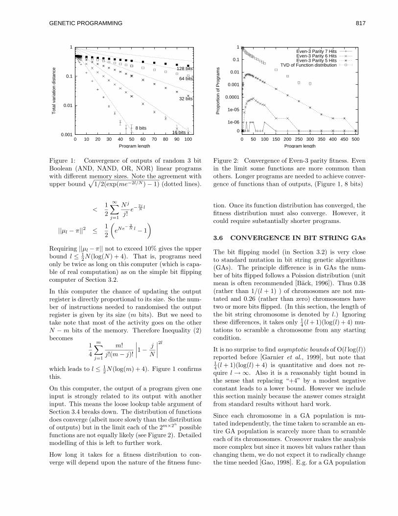
0.001

0.01

0.1

1

0 10 20 30 40 50 60 70 80 90 100

Tot

al v

aria

tion

dist

ance

Program length

8 bits16 bits

32 bits

64 bits

128 bits

Figure 1: Convergence of outputs of random 3 bitBoolean (AND, NAND, OR, NOR) linear programswith different memory sizes. Note the agreement withupper bound

√1/2(exp(me−2l/N )− 1) (dotted lines).

<12

∞∑j=1

N j

j!e−

2jN l

||µl − π||2 ≤ 12

(eNe

− 2N l − 1

)Requiring ||µl−π|| not to exceed 10% gives the upperbound l ≤ 1

2N(log(N) + 4). That is, programs needonly be twice as long on this computer (which is capa-ble of real computation) as on the simple bit flippingcomputer of Section 3.2.

In this computer the chance of updating the outputregister is directly proportional to its size. So the num-ber of instructions needed to randomised the outputregister is given by its size (m bits). But we need totake note that most of the activity goes on the otherN −m bits of the memory. Therefore Inequality (2)becomes

14

m∑j=1

m!j!(m− j)!

∣∣∣∣1− j

N

∣∣∣∣2lwhich leads to l ≤ 1

2N(log(m) + 4). Figure 1 confirmsthis.

On this computer, the output of a program given oneinput is strongly related to its output with anotherinput. This means the loose lookup table argument ofSection 3.4 breaks down. The distribution of functionsdoes converge (albeit more slowly than the distributionof outputs) but in the limit each of the 2m×2n possiblefunctions are not equally likely (see Figure 2). Detailedmodelling of this is left to further work.

How long it takes for a fitness distribution to con-verge will depend upon the nature of the fitness func-

1e-06

1e-05

0.0001

0.001

0.01

0.1

1

0 50 100 150 200 250 300 350 400 450 500

Pro

port

ion

of P

rogr

ams

Program length

0

Even-3 Parity 7 HitsEven-3 Parity 6 HitsEven-3 Parity 5 Hits

TVD of Function distribution

Figure 2: Convergence of Even-3 parity fitness. Evenin the limit some functions are more common thanothers. Longer programs are needed to achieve conver-gence of functions than of outputs, (Figure 1, 8 bits)

tion. Once its function distribution has converged, thefitness distribution must also converge. However, itcould require substantially shorter programs.

3.6 CONVERGENCE IN BIT STRING GAs

The bit flipping model (in Section 3.2) is very closeto standard mutation in bit string genetic algorithms(GAs). The principle difference is in GAs the num-ber of bits flipped follows a Poission distribution (unitmean is often recommended [Back, 1996]). Thus 0.38(rather than 1/(l + 1) ) of chromosomes are not mu-tated and 0.26 (rather than zero) chromosomes havetwo or more bits flipped. (In this section, the length ofthe bit string chromosome is denoted by l.) Ignoringthese differences, it takes only 1

4 (l+ 1)(log(l) + 4) mu-tations to scramble a chromosome from any startingcondition.

It is no surprise to find asymptotic bounds of O(l log(l))reported before [Garnier et al., 1999], but note that14 (l + 1)(log(l) + 4) is quantitative and does not re-quire l→∞. Also it is a reasonably tight bound inthe sense that replacing “+4” by a modest negativeconstant leads to a lower bound. However we includethis section mainly because the answer comes straightfrom standard results without hard work.

Since each chromosome in a GA population is mu-tated independently, the time taken to scramble an en-tire GA population is scarcely more than to scrambleeach of its chromosomes. Crossover makes the analysismore complex but since it moves bit values rather thanchanging them, we do not expect it to radically changethe time needed [Gao, 1998]. E.g. for a GA population


of 32 bit strings, mutation alone (note we turn off se-lection) will scramble it within about 61 generations.(For standard mutation the value may be slightly dif-ferent.) Notice this is independent of population size,in contrast the number of generations taken by selec-tion to unscramble the population depends on the sizeof the population but not l [Blickle, 1996]. Accordingto [Back, 1996, Table 5.4] binary tournament selection(without mutation or crossover) takes only 9 genera-tions to remove all diversity from a population of 100.

4 APPLICABILITY

The results in Section 3 refer to specific types of com-putation, nevertheless we feel they are useful, particu-larly for common varieties of genetic programming.

The model does not cover programs that contain in-structions that are executed more than once. I.e. noloops or backward jumps. (Forward jumps are in prin-ciple acceptable, as long as the number of executedinstructions remains large.) This is, of course, a bigrestriction. However, many problems have been solvedby GP systems without such loops or recursive func-tion calls [Banzhaf et al., 1998]. The difficulty for theproofs is that, in general, repeating (a sequence of) ran-dom instructions does not give, on average, the sameresults as the same number of random instructionschosen independently. (If the loop contains enoughrandom instructions to reach the limiting distributionthen the problem does not arise because the input tothe next iteration to the loop is already in the limitingdistribution and so will remain there.) Similarly, thereis no problem if the loop is followed by a large numberof random instructions.

While the proofs suggests that the program will haltafter l instructions, they can be made slightly moregeneral by extracting the answer from the output reg-ister after l time intervals, allowing the program tocontinue (or to be aborted). These have been called“any time algorithms”. They have been used in GP,e.g. [Teller, 1994].

The dominant factors in determining length requiredfor near convergence are the type of computer consid-ered and the size of its (data) memory. The scalinglaw is given by the type. Comparing the four types inSection 3 suggests that the degree of interconnectionsin the state space is the important factor. The abilityto move directly from one memory pattern to anotherleads to linear scaling, while only being able to moveto 2 adjacent data patterns lead to exponential scal-ing. We suggest that the “bit flipping” and “4 BooleanFunction” models are more typical and so we suggest

O(N logN) would be found on real computers.

Most computers support random access at the byte orword level. This would suggest N should be the num-ber of bytes or words in the data memory. Howeverthen we would expect the individual bits in each byteor word to be highly correlated, and so we would an-ticipate the simple O(N logN) law would break down.I.e. further random instructions will be required to ran-domise them. This might result in a multiplicativefactor of 8 log 8 or 32 log 32 but this yields the samescaling law ((8 log 8)N/8 logN/8 = O(N logN)) pos-sibly with different numerical values.

Some linear GP systems write protect their inputs.The proofs can be extended to cover this by viewingthe read-only register as part of the CPU (i.e. not partof the data memory). Then we get a limiting distribu-tion as before, but it depends on the contents of theread-only register, i.e. the programs’ input. In generalwe would expect this to give the machine a very strongbias (i.e. an asymmetric limiting distribution) and insome cases this might be very useful.

All of the calculations in Section 3 have been explicitlyconcerned with the distribution of answers producedby the programs and the functions implemented bythem. In principle we can use the Markov argumentsto consider the distribution of functions implementedby the programs in other types of computer. TheMarkov process now becomes a sequence of changesin function. We start with the identity function andthe distribution of functions rapidly spreads throughthe 2N

2N

functions. An obvious difficulty is that thesize of the transition matrixes increases exponentially(from 2N × 2N to 2N

2N× 2N2N

). This might lead toan exponential (or worse) increase the upper boundscaling laws.

The random computer (cf. Section 3.4) gives an in-teresting model. Indeed it represents the average be-haviour over all possible computers (of this type).

Finally an alternative view is to treat random instruc-tions as introducing noise. Some instructions, e.g.clear, introduce a lot of noise, while others e.g. NAND,introduce less. So we start with a very strong, noisefree, signal (the inputs) but each random instructiondegrades it. Eventually, in the limiting distribution,there is no information about the inputs left. Thusthe entropy has monotonically increased from zero toa maximum.


5 CONCLUSIONS

The distribution of outputs produced by all comput-ers converges to a limiting distribution as their (linear)programs get longer. We provide a general quantita-tive upper bound (2.31aIa, where I is the number ofinstructions and a is the length programs needed tostore every possible value in the computer’s memory,Section 3.3). Tighter bounds are given for four types ofcomputer. There are radical differences in their con-vergence rates. The length of programs needed forconvergence depends heavily on the type of computer,the size of its (data) memory N and its instruction set.

The cyclic computer (Section 3.1) converges mostslowly, ≤ 0.35 22N , for large N . In contrast the bit flipcomputer (Section 3.2) takes only 1

4 (N+1)(log(m)+4)random instructions (m bits in output register). How-ever in both, the distributions of outputs and of func-tions converge at this same rate to a uniform limitingdistribution.

In Section 3.4 we introduced a random, model of com-puters. This represents the average behaviour over allcomputers (cf. NFL [Wolpert and Macready, 1997]).It takes less than (15.3 + 2.3m)/ log I random instruc-tions to get close to the uniform output limit. Howevera less formal arguments suggests a multiplicative fac-tor of 2n needs to be included before the distributionof functions is also close its limit.

Section 3.5 shows the output of programs comprisedof four common Boolean operators converges to a uni-form distribution within 1

2N(log(m) + 4) random in-structions. The importance of the pragmatic heuristicof write protecting the input register, is highlighted,since without it there are no “interesting” functions inthe limit of large programs.

Section 3.6 shows the number of generations( 1

4 (l + 1)(log(l) + 4)) needed for mutation alone torandomise a bit string GA (chromosome of l bits).

Practical GP fitness functions will converge fasterthan the distribution of all functions, since they typ-ically test only a small part of the whole function.Real GP systems allow rapid movement about thecomputer’s state space and so appear to be close tothe bit flipping (Section 3.2) and four Boolean in-struction (Section 3.5) models. We speculate rapidO(|test set|N logm) convergence in fitness distribu-tions may be observed.

It is ten years since Jaws 1, these are the first generalquantitative scaling laws on the space that genetic pro-gramming searches. They provide theoretical supportfor some pragmatic choices made in GP.

Acknowledgments

I would like to thank Jeffrey Rosenthal, David Corney,Tom Westerdale, James A. Foster, Riccardo Poli, IngoWegener, Nic McPhee, Michael Vose and Jon Rowe.

References

[Back, 1996] Thomas Back. Evolutionary Algorithmsin Theory and Practice: Evolution Strategies, Evo-lutionary Programming, Genetic Algorithms. Ox-ford University Press, New York, 1996.

[Banzhaf et al., 1998] Wolfgang Banzhaf, PeterNordin, Robert E. Keller, and Frank D. Francone.Genetic Programming – An Introduction; On theAutomatic Evolution of Computer Programs andits Applications. Morgan Kaufmann, 1998.

[Blickle, 1996] Tobias Blickle. Theory of Evolution-ary Algorithms and Application to System Synthe-sis. PhD thesis, Swiss Federal Institute of Technol-ogy, Zurich, November 1996.

[Diaconis, 1988] Persi Diaconis. Group Representa-tions in Probability and Statistics, volume 11 of Lec-ture notes-Monograph Series. Institute of Mathe-matical Sciences, Hayward, California, 1988.

[Gao, 1998] Yong Gao. An upper bound on theconvergence rates of canonical genetic algorithms.Complexity International, 5, 1998.

[Garnier et al., 1999] Josselin Garnier, Leila Kallel,and Marc Schoenauer. Rigorous hitting timesfor binary mutations. Evolutionary Computation,7(2):173–203, 1999.

[Langdon and Poli, 2002] W. B. Langdon and Ric-cardo Poli. Foundations of Genetic Programming.Springer-Verlag, 2002.

[Rosenthal, 1995] Jeffrey S. Rosenthal. Convergencerates for Markov chains. SIAM Review, 37(3):387–405, 1995.

[Teller, 1994] Astro Teller. Genetic programming, in-dexed memory, the halting problem, and other cu-riosities. In Proceedings of the 7th annual FloridaArtificial Intelligence Research Symposium, pages270–274, Pensacola, Florida, USA, May 1994. IEEEPress.

[Wolpert and Macready, 1997] David H. Wolpert andWilliam G. Macready. No free lunch theorems foroptimization. IEEE Transactions on EvolutionaryComputation, 1(1):67–82, April 1997.


http://www.csu.edu.au/ci/vol05/gao/grateGao.html

http://www.csu.edu.au/ci/vol05/gao/grateGao.html

http://www.springer.de/cgi-bin/search_book.pl?isbn=3-540-42451-2#english

http://www.cs.cmu.edu/afs/cs/usr/astro/public/papers/Curiosities.ps



Is the Perfect the Enemy of the Good?

Sean LukeGeorge Mason University

http://www.cs.gmu.edu/∼sean/

Liviu PanaitGeorge Mason University

http://www.cs.gmu.edu/∼lpanait/

Abstract

Much of the genetic programming literaturecompares techniques using counts of ideal solu-tions found. These counts in turn form commoncomparison measures such as Koza’s Computa-tional Effort or Cumulative Probability of Suc-cess. The use of these measures continues de-spite past warnings that they are not statisticallyvalid. In this paper we too criticize the mea-sures for serious statistical problems, and also ar-gue that their motivational justification is faulty.We then present evidence suggesting that ideal-solution counts are not necessarily positively re-lated to best-fitness-of-run statistics: in fact theyare often inversely correlated. Thus claims basedon ideal-solution counts can mislead readers intothinking techniques will provide superior finalresults, when in fact the opposite is true.

1 INTRODUCTION

The best is the enemy of the good.— Voltaire (1694–1778)

He who is determined not to be satisfied withanything short of perfection will never do any-thing to please himself or others.— William Hazlitt (1778–1830)

The research methodology in the genetic programming(GP) has many unusual features. Some of these features aregood. Some are not. But we tend to stick with the bad onesout of inertia: we do it that way because others did. Sur-prisingly, the literature does not have a large number of crit-ics of the existing methodology. One notable exception isJason Daida, who has criticized poor random number gen-erator usage [1997], evaluation and verification methodol-ogy [1999a], and historical metaphors [1999b]. Paterson

and Livesey [2000] have decried the poor statistics behindmany claims, noting that many papers do no means testingat all. Angeline [1996] has criticized the statistical reliabil-ity of Koza’s Cumulative Probability of Success measure,a criticism echoed in [Paterson and Livesey 2000].

Here we will continue the criticism of the popular Cumu-lative Probability of Success and other measures based oncounting the number of ideal solutions discovered. Thereare serious statistical flaws with such measures, but thatis not all. These measures also have questionable motiva-tional philosophy, and most importantly, they are poorlycorrelated with other more accepted measures of run qual-ity in the evolutionary computation community.

This paper was born out of experiments for another pur-pose: to test whether fitness might be improved and treesize reduced by increasing the noise of a GP breeding op-erator. The operator chosen was subtree crossover, and itwas made noisier through increasing the number of timestwo parents were crossed over to create a child. Crossingover more times does in fact decrease the mean tree sizeby statistically significant amounts, but it also worsens thebest fitness of the run by a statistically significant margin.But these experiments yielded another odd fact: ideal solu-tion counts were not necessarily tied to fitness results, andin some cases were inversely correlated with them.

The remainder of the paper will discuss common ideal-solution count measures and their statistical weaknesses,and question the motivational philosophy behind them.Then the paper will present the evidence stemming fromthese experiments. The paper then finishes with discussionand recommendations.

2 A TALE OF TWO MEASURES

The non-GP evolutionary computation literature has tra-ditionally compared techniques using the mean best fit-nesses of a large (>30) sample of runs per technique, ac-companied with so-called “best-so-far-curves” (plots of the


mean best fitness discovered so far), plus a t-test1 or otherdifference-of-means test. When generalizability is impor-tant, the mean best fitness results are supplemented withgeneralization ratings on a test set.

Koza [1992] presented a very different metric for comput-ing the “quality” of an evolutionary procedure: how oftenand how rapidly it discovered the ideal solution. From thisdata were derived a variety of statistical metrics ultimatelycomputing how many individuals would need to be evalu-ated before an ideal solution was expected to be found withsome probability.

Koza defined four dependent statistical measures, given asfollows. The instantaneous probability of success measureY (m, i) is the probability that a run with a population size ofm will discover an ideal solution for the first time on gen-eration i. From this it is simple to determine P(m, i), thecumulative probability of success, which is the probabilitythat a run will discover an ideal solution before or on gener-ation i. Koza writes R(m, i,z) as the number of evolutionaryruns required to have a probability z = 99% of discoveringa solution before generation i. He defines this as

R(m, i,z) =

⌈

log(1− z)log(1−P(m, i))

⌉

Sometimes this is shortened to just R(z). The individuals tobe processed measure I(m, i,z) is then defined straightfor-wardly as I(m, i,z) = m(i + 1)R(m, i,z), at least for gener-ational evolutionary procedures. The computational effortmeasure E is the minimum of I(m, i,z) over all values of i.

Ideal-solution count measures have since taken root in theGP community. Of these four, the two most common mea-sures in the literature are Cumulative Probability of Suc-cess, for which higher values are better, and its derivedmeasure Computational Effort, for which lower values arebetter. We performed an informal survey of the genetic pro-gramming and evolvable hardware non-poster papers in thethree GECCO conferences so far (1999, 2000, 2001). Ofthese, 44 compared two or more techniques for solutionquality. Eighteen compared the mean best fitness of runbetween techniques.2 Twelve instead used statistics basedon the number of ideal solutions discovered (most used the

1The validity of the t-test and ANOVA for GP were examinedin [Paterson and Livesey 2000]. As the t-test and ANOVA assumenormality, the authors had expected to find them wanting in theGP realm, but astonishingly they significantly outperformed non-parametric tests. Even so, the authors warned about the dangers ofrelying too much on t-tests for the skewed distributions commonto GP. We agree! Still, we think that t-tests and ANOVAs shouldat least be the bare minimum for means testing in GP.

2Of the eighteen experiments which used fitness curves tocompare techniques, only seven used good statistics. The othereleven had sample sizes that were too small (much less than 30)or unreported, or they did not indicate statistical significance re-sults or variance information. One of us (Sean Luke) hastens to

Koza measures). Fourteen used a train/test methodologyborrowed from the machine learning community: typicallythey measured how long it took to discover a perfect solu-tion to a training set, then tested generalization ability.3

We feel there are three problems with ideal-solution countmeasures. First, they rely on unacceptably poor statistics, atleast as generally practiced in the community, and to rem-edy this would require a very large sample size. Second,they are founded on, in our opinion, an unclear motiva-tional philosophy. The third problem, and most troubling,is that they appear to be uncorrelated with best-fitness-of-run comparisons. These problems call a fair chunk of theliterature into question.

2.1 STATISTICAL PROBLEMS

Ideal solution count measures are statistically suspect.

First, the measures are based on a single point sample ofthe number of ideal solutions and the generations in whichthey were found. A point sample does not have a meantest: there is no accepted procedure to state that two suchsamples differ in a statistically significant way.

The point sample difficulty might be alleviated by doinga large number of runs, then dividing them into at leastthirty piles, then counting the ideal solutions in each pileand using the mean number of ideal solutions per pile as asample statistic. For Symbolic Regression this is feasible,as a large number of runs end in perfect solutions. But formany problem domains, ideal solutions are typically fewand far between. In this paper we gathered samples of fivehundred each, typically five to ten times the number foundin most of the experimental literature. And still, the ideal-solution counts for the Artificial Ant and 11-Bit BooleanMultiplexer were so small (at most sixteen and twelve re-spectively) that dividing into piles was not doable.

Second, several of the measures are statistically dependentacross generations. For example, to truly compute statisti-cally independent Cumulative Probability of Success mea-sures for both generation 4 and for generation 8 would re-quire two separate, independent samples.

Third, changes in the Individuals to be Processed mea-sure and its derived Computational Effort measure are bothgreatly exaggerated when small changes occur in ideal so-

note that he too has published papers with statistical difficulties,though in his defense they were either corrected ([Luke and Spec-tor 1997] fixed in [Luke and Spector 1998]) or openly acknowl-edged and justified in the paper itself [Luke 2001b].

3As many machine learning algorithms are deterministic, theydo not require statistical mean tests. This is not true for stochasticevolutionary computation algorithms: yet relatively few train/testmethodology papers in this survey presented statistical signifi-cance results.


lution counts. For example, note that the ComputationalEffort in Figure 12 is a strongly nonlinear function of thenumber of ideal solutions found, shown in Figure 10.

To overcome all the statistical problems detailed herewould require multiple independent samples across gener-ations, plus dramatically larger sample sizes for the moredifficult domains. We feel these statistical flaws would beforgivable only if ideal-solution counts were the only feasi-ble way to compare techniques. But they are not.

2.2 MOTIVATIONAL PHILOSOPHY

The evaluation functions used in the assessment of a GPindividual’s fitness do not correspond well to a stated goalof an ideal-solution end result. GP optimizes for as good afitness as it can get, not for increasing probability of attain-ing the ideal. Many GP problem domains are highly de-ceptive, leading the evolutionary trajectory away from theideal rather than toward it. Consider the Symbolic Regres-sion domain: if the ideal solution is not found early on, andthe population has fixated on certain near-solutions, it willcontinue to tack on code to the bottom of trees which canmake the solutions only incrementally fitter. Many Sym-bolic Regression runs will ultimately generate very largetrees with solutions very close to the answer, but far (inmakeup) from anything remotely resembling the answer.

Given this, and given the statistical problems behind ideal-solution count measures, what is the GP community’s mo-tivational justification for using ideal-solution counts at all?We believe that counts are popular because of a philo-sophical conceit that GP operates over problem domainswhich demand correct programs. More generally this canbe thought of as an absolute hard constraint on the desiredoutcome: either the program works or it doesn’t work, anda highly fit but suboptimal solution is not valuable. A termpeculiar to GP, “discovery”, reinforces this notion: eitherGP “discovers” the answer, or it doesn’t.4

4In fact, though his influential text introduced the ideal-solution count measures discussed in this paper, Koza couchedhis support of this philosophy, writing:

“Several pages ago, when I spoke of writing a computer pro-gram to center the cart in optimal time, you probably assumed thatI was talking about writing a correct computer program to solvethe problem. Nothing could be further from the truth. In fact, thisbook focuses almost entirely on incorrect programs. In particular,I want to develop the notion that there are gradations in perfor-mance among computer programs. Some incorrect programs arevery poor; some are better than others; some are approximatelycorrect; occasionally, one may be 100% correct. Expressing thisbiologically, one could say that some computer programs are fit-ter than others in their environment. It is rare for any biologicalorganism to be optimal.” [Koza 1992, p. 130]

Regression 3 2 4 1 5 6 7 10 8 9

Multiplexer 2 1 3 4 5 6 7 8 9 10

Ant 2 1 4 6 3 5 7 8 9 10

Table 1: Statistical significance groupings for the meanbest-fitness-of-run for each problem domain, using theTukey post-hoc ANOVA test. Numbers indicate the num-ber of crossovers for a given multi-crossover technique.Techniques are ordered by increasing (poorer) mean best-fitness-of-run. Bars connect techniques with statisticallyinsignificant differences in means among them. Note thatmore crossovers generally results in worse mean best-fitness-of-run. Compare to Figures 1, 5, and 9.

It is clear that there exist valid and important GP prob-lem domains where discovery is of paramount importance.However, we believe that many, and likely most, new prob-lems in GP rarely require 100% correctness as a necessaryattribute. These problems include neural networks, molec-ular structures, soccer softbot programs, probabilistic andquantum algorithms, analog electrical circuits, etc. Theprimary reason for this, we think, is that these new do-mains are significantly harder and their optima are oftenunknown. Discovering the optimum, and particularly dis-covering it enough times to make statistical conclusions, isa luxury usually reserved for only the simplest of problemdomains.

We are now out of the proof-of-concept period for GP. Forthe technique to now be used realistically as a tool, we mustassume it will typically be used to attack hard problems forwhich we do not know the optimum, do not expect it to dis-cover the optimum, nor even know if there is an optimum.An engineer would ask: if we already know the answer,why bother to use GP to find it? What matters is not if tech-nique A finds more perfect solutions than technique B doesto Easy Problem C. What usually matters is that techniqueA gets a better answer than B does for Hard Problem D.We submit that if one can “discover” the optimum enoughtimes to validly measure the performance of a techniqueagainst a given problem domain, then we are dealing witha toy problem.

If past literature used a weak methodology, we should dis-continue its use. Nonetheless, we recognize that for thoseproblems which demand perfection, ideal-solution-countstatistics may have some usefulness. Later in this paper wewill recommend experimental protocols which may incor-porate ideal solution counts as one part of a comprehensiveanalysis. At the same time, we will propose an alternativewhich we think provides more useful information.


1 2 3 4 5 6 7 8 9 10Number of Crossovers

0

0.5

1

1.5

2

2.5

3

Bes

tFitn

ess

ofR

un

Figure 1: Boxplots of the distribution of best-fitness-of-run, by number of crossovers, Symbolic Regression do-main. Lower fitness is better. Compare to Table 1.


150

200

250

300

Num

ber

ofId

ealS

olut

ions

Figure 2: Number of ideal solutions found, by number ofcrossovers, Symbolic Regression domain.

3 A TROUBLING LACK OFCORRELATION

At first it seems intuitive that a system which searches bet-ter for high-fitness solutions would also tend to find moreideal solutions. An experiment gone awry shows us that infact this is not necessarily the case.

The experiment we performed applied what we call multi-crossover to GP. Ordinarily GP crossover selects two indi-viduals, and performs one swap of randomly-chosen sub-trees, producing two children. If a child passes validityconstraints (such as maximal depth), it then enters the nextgeneration; otherwise a copy of the child’s mother entersin its stead. Multi-crossover is simply a composition of GPcrossover operators: two parents are selected and crossoveris performed, including validity constraints. Then the chil-dren become the “parents” for the next crossover operator,which produces two new children. This happens N times,then the final results enter the next generation.

We had two reasons for doing multi-crossover experiments.First, some models of code bloat (our own depth-basedtheory [Luke 2000], Defense Against Crossover [Banzhafet al. 1998], and Removal Bias [Langdon et al. 1999]) as-sume that there is a single crossover per individual; hence

1020

3040

50

Generation

1

23

45

67

89

10

Crossovers

0

0.2

0.4

0.6CumulativeProbabilityof Success

1020

3040

50

Generation

Figure 3: Cumulative Probability of Success per genera-tion, by number of crossovers, Symbolic Regression do-main.


6000

7000

8000

9000

10000

11000

Effo

rt

Figure 4: Computational Effort by number of crossovers,Symbolic Regression domain.

the probabilities of choosing crossover point A or B respec-tively were not independent. While increasing the num-ber of crossover events would not break this dependency, itcould lower the effect the dependency had in causing bloat.

Second, adding more nonhomologous crossover eventsmeant adding more variation (more noise) into the breed-ing procedure. This gave us a dial to turn which would ef-fectively change the amount that crossover “randomized”individuals (an idea inspired by arguments made in [An-geline 1997]). Would more randomization be beneficial ordetrimental to GP?

The experiments were done as follows. We ran for 51 gen-erations, including the initial generation, using a populationof 500, and tournament selection of size 7. Multi-crossoverwas the sole operator used. The three problem domainschosen were Symbolic Regression, 11-Bit Boolean Mul-tiplexer, and Artificial Ant. Symbolic Regression usedno Ephemeral Random Constants. Artificial Ant used theSanta Fe Trail. All other run and problem domain param-eters were done as stipulated in [Koza 1992]. The evolu-tionary computation system used was ECJ [Luke 2001a].



0

100

200

300

400

500

600

700

Bes

tFitn

ess

ofR

un

Figure 5: Boxplots of the distribution of best-fitness-of-run, by number of crossovers, 11-Bit Boolean Multiplexerdomain. Lower fitness is better. Compare to Table 1.


2

4

6

8

10

12

Num

ber

ofId

ealS

olut

ions

Figure 6: Number of ideal solutions found, by number ofcrossovers, 11-Bit Boolean Multiplexer domain.

We performed ten different experiments, with multi-crossover set to 1 through 10 crossovers respectively. Eachexperiment consisted of 500 independent runs. This num-ber of runs is much higher than is necessary to producebest-fitness-of-run results, but we needed as many runs aspossible to feel at least partially confident in our ideal-solution counts, and 15,000 total runs was the most wecould afford to do. For each problem domain we used box-plots5 to plot best-fitness-of-run distributions for differentnumbers of crossovers. We also plotted the number of idealsolutions found, and the Cumulative Probability of Successand Computational Effort measures.

3.1 SYMBOLIC REGRESSION RESULTS

Symbolic Regression did in fact lower tree size. But it didso at the cost of a statistically significant worsening of fit-ness, though only gradually: large swaths of crossover ex-periments were in the same statistical equivalence class, asshown in Table 1. Increasing the amount of noise in thecrossover procedure, thus moving the system more towards

5In a boxplot, the rectangular region covers all values betweenthe first and third quartiles, the stems mark the furthest individualwithin 1.5 of the quartile ranges, and the center horizontal lineindicates the median. Dots show outliers, and × marks the mean.

1020

3040

50

Generation

12

34

56

78

910

Crossovers

0

0.005

0.01


1020

3040

50

Generation

Figure 7: Cumulative Probability of Success per genera-tion, by number of crossovers, 11-Bit Boolean Multiplexerdomain.


1· 106

2· 106

3· 106

4· 106

5· 106

Effo

rt

Figure 8: Computational Effort by number of crossovers,11-Bit Boolean Multiplexer domain.

random search, yielded worse results on average, using themean best-fitness-of-run measure as shown in Figure 1.

But one would not have known this from the ideal-solutioncounts. As noise in crossover increased, the number ofideal solutions increased rapidly from 150 per 500 runswith a single crossover, to stabilizing at about 350 per 500runs with seven crossovers or more, as shown in Figure 2.This in turn resulted in an unexpected Cumulative Proba-bility of Success curve, and a major decrease in Compu-tational Effort as the number of crossovers increased, asshown in Figures 3 and 4.

Symbolic Regression is the easiest of the three problem do-mains presented: it finds the ideal solution very often (noless than 30% of the time in these experiments). Thus ourcounts were very high and the Cumulative Probability ofSuccess curve was very smooth.

This outcome was very disturbing. Were we to have usedideal-solution count measurements as our basis of compar-ison in this experiment, our conclusions wouldn’t just havebeen uncorrelated with best-fitness-of-run results: they



0

10

20

30

40

50

Bes

tFitn

ess

ofR

un

Figure 9: Boxplots of the distribution of best-fitness-of-run,by number of crossovers, Artificial Ant domain. Lower fit-ness is better. Compare to Table 1.


2

4

6

8

10

12

14

16

Num

ber

ofId

ealS

olut

ions

Figure 10: Number of ideal solutions found, by number ofcrossovers, Artificial Ant domain.

would have been the opposite. We would have concludedthat increasing number of crossovers does a better job.

3.2 11-BIT BOOLEAN MULTIPLEXER RESULTS

11-Bit Boolean Multiplexer was to yield another surprise.First, it too lowered tree size, and like Symbolic Regres-sion, it did so by statistically significantly worsening the fit-ness results. Again, increasing the amount of noise yieldedworse results on average, when using the mean best-fitness-of-run measure, as shown in Figure 5. This time, the fit-nesses worsened rapidly, with few in the same statisticalequivalence class, as seen in Table 1.

Given its tendency to bloat like Regression does, wefully expected Multiplexer to have similar ideal-solutioncounts. But this was not quite the case. As the numberof crossovers increased, the number of ideal solutions in-creased, but then it then decreased again. Multiplexer is arelatively more difficult problem domain to find ideal so-lutions in: thus we found no more than thirteen ideal so-lutions in 500 runs, with the maximum peaking when weapplied five crossovers. The nadir was a single solutiondiscovered, when we applied nine crossovers, as shown inFigure 6.

1020

3040

50

Generation

12

34

56

78

910

Crossovers

0

0.01

0.02


1020

3040

50

Generation

Figure 11: Cumulative Probability of Success per genera-tion, by number of crossovers, Artificial Ant domain.


500000

1· 106

1.5· 106

2· 106

2.5· 106

3· 106

3.5· 106

4· 106

Effo

rt

Figure 12: Computational Effort by number of crossovers,Artificial Ant domain.

The Cumulative Probability of Success similarly followeda bell curve distribution, as is shown in Figure 7. Therelatively low number of ideal solutions resulted in theexpected exaggerated swings in Computational Effort, asshown in Figure 8.

Here, while a best-fitness-of-run measure would statethat increasing crossovers generally decreased quality, anideal-solution count measure would argue that increasingcrossovers somewhat (to five) made the result twice asgood.

3.3 ARTIFICIAL ANT RESULTS

Artificial Ant gave us yet another result. Again, it low-ered tree size, and once again, it also did so by statisti-cally significantly worsening the fitness results (Figure 9)though like Symbolic Regression the results worsened onlyslightly, resulting in large numbers of experiments in thesame statistical equivalence class (Table 1).

Figure 10 reveals that this time, the ideal-solution countsfollowed the statistically significant fitness: increasing theamount of noise decreased the number of ideal solutions


discovered. As shown in Figure 11, the Cumulative Prob-ability of Success followed a radically different curve thanwas the case in Symbolic Regression. Like Multiplexer,Artificial Ant discovers relatively few ideal solutions (nomore than sixteen out of 500). And like Multiplexer, thisexaggerates the Computational Effort results (Figure 12).

Here, as in Symbolic Regression, one would conclude onthe basis of the best-fitness-of-run measure that the mean isgetting just a little worse, though statistically significantly.But here an ideal-solution-count measure suggests that in-creasing the number of crossovers considerably worsensthe result.

4 WHAT’S GOING ON?

For all three problems, fitness gradually worsened as thenumber of crossovers increased. But each problem yieldeda wildly different result in the ideal-solutions count, andthus in the Cumulative Probability of Success and Compu-tational Effort metrics. In short, the ideal-solution countswere not correlated with the best-fitness-of-run measure.

We think the reason for this phenomenon is that, as shownin Figures 1, 5, and 9, the number of ideal solutions is moreclosely linked to the variance of — rather than the mean of— the best-fitness-of-run distribution. As the variance in-creases, fitness is increasingly scattered both up and down.But there is a bound at zero (one cannot be better than per-fect), whereas there is no bound on getting worse. Thus awider variance tends to rack up more perfect scores. Thistrend is echoed in the data for all three problem domains,although the ideal-solution counts in the Artificial Ant andMultiplexer domains are low enough to make us wary aboutmaking a pronouncement.

In the Symbolic Regression domain, the distributions areskewed. As the number of crossovers increases, the meanincreases a little, but not nearly as much as the variancedoes. Thus a worsening in the mean is not able to pre-vent ideal solutions from piling up. In the Multiplexer do-main, the mean worsens only a little initially but rapidlyat the end, while the variance generally increases steadily.This allows the mean to lose to, then catch up with thevariance, which might explain the ideal-solution counts.Lastly, the Artificial Ant domain’s mean worsens slowlywhile the variance decreases, which can explain the steadydecrease in ideal-solution counts.

This combination of mean and variance has a closely re-lated effect: even if low-variance technique A has a higherexpected value than high-variance technique B for a singlerun, B can still have a higher expected best result of N inde-pendent runs (Figure 13). This phenomenon was exploredin [Luke 2001b].

Figure 13: Example of two distributions which differ inmean and in variance. While one sample from the flatterdistribution will give a lower expected result (the mean)than the tall distribution, in this case the best of two or moresamples from the flatter distribution will give a higher ex-pected result.

We will not venture a guess as to why increasing the num-ber of crossovers changed the mean and variance results inthe way it did. We had expected that increasing the numberof crossovers would consistently increase the variance, butclearly it does not.

Regardless of the outcome, we do not believe that these ex-periments bode well for the body of GP literature whichrelies on ideal-solution counts to compare the quality ofdifferent techniques. We are concerned that upon readingthis literature, experimenters may mistakenly conclude thatcertain techniques are better than others on average, whenin some cases better ideal-solution counts are actually in-dicative of a worse result in mean best-fitness-of-run.

5 RECOMMENDATIONS

One downside to mean-best-fitness-of-run results isdemonstrated in the Symbolic Regression domain: tech-niques which produce large, bloated trees that are function-ally “close” to the ideal are given high marks, even thoughthe results do not remotely resemble our notion of what theideal individual ought to look like. Ideal-solution countscan be somewhat useful here in weeding these pretendersout. But given their statistical problems, we feel that ideal-solution count results alone simply cannot be justified.

If such incrementalism is the critical sticking-point tempt-ing an author to only report ideal-solution counts, we sug-gest instead that the author produce results showing bothmean best fitness of run and mean tree size. If a tech-nique is superior both in tree size and mean best fitness, it ismore difficult to argue that the improvements in mean best-fitness-of-run are due to incrementalism, since this wouldlikely also increase tree size. Another approach would be


to change the methodology to one showing generalization,using training and testing sets. Incrementalism tends to re-sult in solutions custom-tailored to the training set: suchpoor generalizability would then show up when the finalsolution is compared to the testing set.

If instead one were performing runs in a domain which de-manded perfection, then it would obviously be useful toknow how often a technique was likely to find the ideal so-lution. Another situation also commonly arises: trying tobeat an existing record, where it’s useful to know not if atechnique is likely to find the ideal, but whether or not it islikely to find any solution better than the record. In thesesituations we suggest that counts could supplement, but notreplace, the mean best-fitness-of-run results.

But for most cases we suggest a different point statisticto use as a supplement. The procedure specified in [Luke2001b] gives the expected maximum best-fitness-of-run forN total runs. This procedure, like the ideal-solution-countprocedure, suffers statistically from the assumption that thesample is exactly representative of the population, and fromits reuse of statistically dependent data. However, as a sup-plement to mean best-fitness-of-run results, we think it is amore useful metric than ideal solution counts in most cases.

The procedure is as follows. Perform a large number m runsfor a given technique T . Sort the runs by fitness and assignranks 1, ...,m to the runs, where rank 1 is the worst-fitnessrun for the technique. Let F(r) be the fitness of the runranked r. Then if one were to perform N runs and returnthe best run, the expected best fitness E(T,N) among thoseN runs would be:

E(T,N) =

m∑

r=1

F(r)rN − (r−1)N

mN

This presumes that higher fitness values are better. Nowconsider two techniques A and B, where beyond some pointN ≥C, E(B,N) is consistently greater than or equal toE(A,N). Ideally, C would be 1. This would lend evidenceto the belief that not only is A better than B on average, butit is also superior no matter how many runs you are likelyto perform. This gives strong weight to the claim that Areally is better than B. Further, it seems likely that if tech-nique A finds many more ideal solutions than techniqueB, that E(A,N) will surpass E(B,N) above some point Nwhere finding ideal solutions with A becomes sufficientlycommon.

In any case, given their grievous statistical problems, westrongly urge that an ideal solution count measures neverbe used alone as proof that one technique is superior toanother, except under special circumstances and with theappropriate disclaimers. If used at all, they should be onlyused to bolster a more statistically viable fitness compari-son procedure.

Last, we recommend that experimenters more closely adoptdifference-of-means tests (at least t-tests and ANOVAs),and a reasonable sample size (30 at a minimum) in pub-lished evolutionary computation experiments, or give justi-fications for doing otherwise.

6 CONCLUSION

Many papers in the GP literature use ideal-solution countsin one way or another, usually to compare the quality oftechniques. This notion was popularized by Koza’s Cumu-lative Probability of Success, Individuals to be Processed,and Computational Effort measures. This use continues de-spite warnings that counts are poor estimates, as they are apoint statistic with no associated means test; as they makeassumptions about dependencies across generations; and asthey are exaggerated by small count sizes.

In this paper we reiterated this warning about counts, andnoted motivational concerns. Specifically, we noted that formost “difficult” problems, the goal is to find as good a so-lution as possible. Counting the number of times the idealsolution is found does not help achieve this goal. Further,if one can find the ideal reliably, then the problem is trivial.

We also demonstrated the disturbing fact that ideal solutioncounts are not well correlated with mean best-of-fitnessmeasures. In fact, for some problem domains, we showedthat ideal solution counts may lead to the opposite conclu-sion that mean best-of-fitness measures lead to. This begsa reevaluation of much of the GP literature, as publishedresults may be dubious, and in some cases the opposite oftheir intended meaning.

Acknowledgments

Our thanks to Lee Spector, Paul Wiegand, and Ken De Jongfor their insights and responses, and to our reviewers fortheir helpful comments.

References

Angeline, P. J. (1996). An investigation into the sensitiv-ity of genetic programming to the frequency of leaf se-lection during subtree crossover. In Koza, J. R., Gold-berg, D. E., Fogel, D. B., and Riolo, R. L., editors, Ge-netic Programming 1996: Proceedings of the First An-nual Conference, pages 21–29, Stanford University, CA,USA. MIT Press.

Angeline, P. J. (1997). Subtree crossover: Building blockengine or macromutation? In Koza, J. R., Deb, K.,Dorigo, M., Fogel, D. B., Garzon, M., Iba, H., and Riolo,R. L., editors, Genetic Programming 1997: Proceedings


of the Second Annual Conference, pages 9–17, StanfordUniversity, CA, USA. Morgan Kaufmann.

Banzhaf, W., Nordin, P., Keller, R. E., and Francone, F. D.(1998). Genetic Programming – An Introduction; Onthe Automatic Evolution of Computer Programs and itsApplications. Morgan Kaufmann, dpunkt.verlag.

Daida, J., Ross, S., McClain, J., Ampy, D., and Holczer,M. (1997). Challenges with verification, repeatability,and meaningful comparisons in genetic programming. InKoza, J. R., Deb, K., Dorigo, M., Fogel, D. B., Garzon,M., Iba, H., and Riolo, R. L., editors, Genetic Program-ming 1997: Proceedings of the Second Annual Confer-ence, pages 64–69, Stanford University, CA, USA. Mor-gan Kaufmann.

Daida, J. M., Ampy, D. S., Ratanasavetavadhana, M., Li,H., and Chaudhri, O. A. (1999a). Challenges with verifi-cation, repeatability, and meaningful comparison in ge-netic programming: Gibson’s magic. In Banzhaf, W.,Daida, J., Eiben, A. E., Garzon, M. H., Honavar, V.,Jakiela, M., and Smith, R. E., editors, Proceedings of theGenetic and Evolutionary Computation Conference, vol-ume 2, pages 1851–1858, Orlando, Florida, USA. Mor-gan Kaufmann.

Daida, J. M., Yalcin, S. P., Litvak, P. M., Eickhoff, G. A.,and Polito, J. A. (1999b). Of metaphors and darwinism:Deconstructing genetic programming’s chimera. In An-geline, P. J., Michalewicz, Z., Schoenauer, M., Yao, X.,and Zalzala, A., editors, Proceedings of the Congress onEvolutionary Computation, volume 1, pages 453–462,Mayflower Hotel, Washington D.C., USA. IEEE Press.

Koza, J. R. (1992). Genetic Programming: On the Pro-gramming of Computers by Means of Natural Selection.MIT Press, Cambridge, MA, USA.

Langdon, W. B., Soule, T., Poli, R., and Foster, J. A.(1999). The evolution of size and shape. In Spector, L.,Langdon, W. B., O’Reilly, U.-M., and Angeline, P. J.,editors, Advances in Genetic Programming 3, chapter 8,pages 163–190. MIT Press, Cambridge, MA, USA.

Luke, S. (2000). Issues in Scaling Genetic Programming:Breeding Strategies, Tree Generation, and Code Bloat.PhD thesis, Department of Computer Science, Univer-sity of Maryland, A. V. Williams Building, University ofMaryland, College Park, MD 20742 USA.

Luke, S. (2001a). ECJ 7: An evolutionary computationresearch system in Java. Available athttp://www.cs.umd.edu/projects/plus/ec/ecj/.

Luke, S. (2001b). When short runs beat long runs. InSpector, L., Goodman, E. D., Wu, A., Langdon, W. B.,Voigt, H.-M., Gen, M., Sen, S., Dorigo, M., Pezeshk, S.,Garzon, M. H., and Burke, E., editors, Proceedings ofthe Genetic and Evolutionary Computation Conference

(GECCO-2001), pages 74–80, San Francisco, Califor-nia, USA. Morgan Kaufmann.

Luke, S. and Spector, L. (1997). A comparison of crossoverand mutation in genetic programming. In Koza, J. R.,Deb, K., Dorigo, M., Fogel, D. B., Garzon, M., Iba, H.,and Riolo, R. L., editors, Genetic Programming 1997:Proceedings of the Second Annual Conference, pages240–248, Stanford University, CA, USA. Morgan Kauf-mann.

Luke, S. and Spector, L. (1998). A revised compari-son of crossover and mutation in genetic programming.In Koza, J. R., Banzhaf, W., Chellapilla, K., Deb, K.,Dorigo, M., Fogel, D. B., Garzon, M. H., Goldberg,D. E., Iba, H., and Riolo, R., editors, Genetic Program-ming 1998: Proceedings of the Third Annual Confer-ence, pages 208–213, University of Wisconsin, Madison,Wisconsin, USA. Morgan Kaufmann.

Paterson, N. and Livesey, M. (2000). Performance com-parison in genetic programming. In Whitley, D., editor,Late Breaking Papers at the 2000 Genetic and Evolu-tionary Computation Conference, pages 253–260, LasVegas, Nevada, USA.


Lexicographic Parsimony Pressure

Sean LukeGeorge Mason University

http://www.cs.gmu.edu/∼sean/

Liviu PanaitGeorge Mason University

http://www.cs.gmu.edu/∼lpanait/

Abstract

We introduce a technique called lexicographicparsimony pressure, for controlling the signifi-cant growth of genetic programming trees dur-ing the course of an evolutionary computationrun. Lexicographic parsimony pressure modifiesselection to prefer smaller trees only when fit-nesses are equal (or equal in rank). This tech-nique is simple to implement and is not affectedby specific differences in fitness values, but onlyby their relative ranking. In two experiments weshow that lexicographic parsimony pressure re-duces tree size while maintaining good fitnessvalues, particularly when coupled with Koza-style maximum tree depth limits.

1 INTRODUCTION

Like many arbitrary-sized representations in evolutionarycomputation, genetic programming (GP) individuals tendto grow significantly in size when no code growth counter-agents are applied. This growth is relatively independent ofsignificant increases in fitness. The phenomenon, known inGP circles as bloat, is shaping up to be a major impedi-ment to GP’s scalability to more difficult problems whichnecessitate longer evolutionary runs.

The chief way bloat is controlled in GP is through theuse of breeding restrictions stipulating the maximum depthof a GP parse tree individual. Lately other approacheshave taken root, most popularly various forms of parsi-mony pressure, where the size of an individual is taken intoconsideration during selection. Parsimony pressure has todate taken two basic forms: parametric parsimony pres-sure, where an individual’s size directly changes its fitness,and pareto parsimony pressure, where an individual’s sizeis considered as an additional objective in a pareto opti-mization scheme.

In this paper we present a new family of parsimony pres-sure techniques which we think may be particularly apro-pos to GP and other evolutionary systems with large num-bers of fitness-equivalent individuals in a population. Thisfamily is collectively known as lexicographic parsimonypressure, and is based on the idea of placing fitness, thensize in lexicographic order; that is, preferring smaller indi-viduals only when fitness is identical (or in some versions,similar). Lexicographic parsimony pressure is simple toimplement, and it is less tied to the specific absolute fit-ness values in the population than parametric techniquesare, much in the same way that tournament selection toutedover fitness-proportionate selection.

We open the paper with discussions of current bloat-controltechniques, followed by a description of lexicographic par-simony pressure and variations we have tried. We then givethe results of an experiment showing that in most cases lex-icographic parsimony pressure produces equivalent best-fitness-of-run results with significantly smaller trees thandoes depth restriction, except in the Symbolic Regressiondomain, where it performs poorly. We then give the re-sults of a second experiment where we show that combina-tions of lexicographic parsimony pressure and depth limit-ing work very well compared to depth limiting alone.

2 CONTROLLING BLOAT

The evolutionary computation community has tried a num-ber of approaches to controlling the growth of arbitrary-sized individuals. First and foremost are a number of parsi-mony pressure techniques, which include consideration ofan individual’s size as part of the selection procedure. Ge-netic programming has popularized some other techniques.Below we list four such techniques, followed by a range ofparsimony pressure approaches.

Maximum Size or Depth Restriction This approachsimply limits the maximum size of an individual, usuallyby rejecting large children as part of the breeding process.


For example, much work in GP follows the technique usedin Koza [1992], which restricts modification operators toproduce new trees of depth less than 17.

Explicitly Defined Introns This GP-specific techniqueallows the inclusion of special nodes which adapt the likeli-hood of subtree crossover or mutation at specific positionsin the tree [Nordin et al. 1996].

Code Editing One easy way to attack growth is to di-rectly simplify and optimize an individual’s parse tree.Soule et al. [1996] for example report strong results withthis approach. However, Haynes [1998] warns that editingcan lead to premature convergence.

Pseudo-Hillclimbing This technique rejects children ifthey are not superior to (or simply different from) their par-ents in fitness. If a child is rejected from joining the nextgeneration, a copy of its parent joins the next generation inits stead. One effect of this technique is to replicate largenumbers of parents into future generations; earlier individ-uals are generally smaller than later individuals (hence thebloat), this results in slower growth in average size. Thistechnique has been reported with some success in [Lang-don and Poli 1998; Soule and Foster 1998b].

2.1 PARSIMONY PRESSURE

Unlike the techniques mentioned earlier, parsimony pres-sure is not GP-specific and has been used wheneverarbitrary-sized representations tended to get out of hand.Such usage to date can be divided into two broad cate-gories: parametric parsimony pressure, where size is a di-rect numerical factor in fitness, and pareto parsimony pres-sure, where size is considered as a separate objective in apareto-optimization procedure.

Parametric Parsimony Pressure This includes sizemetrics, along with raw fitness, as part of an equation incomputing the final fitness of an individual. For purposes ofthe discussion, let f be the individual’s raw fitness, wherehigher is better, and g be the fitness after parsimony pres-sure is considered. Let s be an individual’s size, and leta,b,c be arbitrary constants.

The most widely-used approach to parametric parsimonypressure is to treat the individual’s size as a linear factor infitness, that is, g = a f − bs. This technique has been usedin both GP [Koza 1992] and in non-GP [Burke et al. 1998].Soule and Foster [1998a] present an interesting analysis oflinear parsimony pressure and when and why it can fail.Linear parsimony pressure is occasionally augmented witha limit, that is if s� c then g = a f , else g = a f + b(c− s)[Cavaretta and Chellapilla 1999]. Belpaeme [1999] used a

similar limit, but considered maximal tree depth rather thansize as the parameter. Nordin and Banzhaf [1995] also ap-plied parametric parsimony pressure, believed to be linear,to evolve machine language GP strings.

Linear parsimony pressure has been used in combina-tion with adaptive strategies. Zhang and Muhlenbein[1995] adjusted b based on current population quality. Ibaet al. [1994] propose a similar technique, except they useinformation-theoretic functions for f and s. Linear par-simony pressure has also been applied in stages: first bysetting g = f , then factoring in size only after the pop-ulation has reached a sufficient quality [Kalganova andMiller 1999]. Some non-GP papers [Wu et al. 1999; Bas-sett and De Jong 2000] use a nonlinear parsimony pressure:g = (1− as) f . Bassett and De Jong note that this has theadded feature of increasing the penalty proportionally tothe fitness.

The problem with parametric parsimony pressure is exactlythat: it is parametric, rather than based on rank. One musttune the parsimony pressure so as not to overwhelm thefitness metric. This can be difficult when the fitness as-sessment procedure is nonlinear, as is usually the case: itmay well be that a difference between 0.9 and 0.91 in fit-ness is much more significant than a difference between0.7 and 0.9. Parametric parsimony pressure can thus givesize an unwanted advantage over fitness when the differ-ence in fitness is only 0.01 as opposed to 0.2. Unexpectedstrength in the size parameter can also arise when the pop-ulation’s fitnesses are converging late in the evolution pro-cedure. These issues are similar to those which gave riseto the preference of tournament selection and other non-parametric selection procedures over fitness-proportionateselection.

Pareto Parsimony Pressure The recent trend in parsi-mony pressure has been to treat it as a separate objective ina nonparametric, pareto optimization scheme. Pareto opti-mization is used when the evolutionary system must opti-mize for two or more objectives at once, but it is not clearwhich objective is “more important”. An individual A issaid to pareto-dominate another individual B if A is as goodas B on all objectives, and better than B in at least one ob-jective. One pareto optimization scheme assumes that oneindividual has a higher fitness than another if it dominatesthe other. Another scheme bases the fitness of individualson the number of other individuals they dominate.

Pareto parsimony pressure treats raw fitness as one objec-tive to optimize, and the individual’s size as another objec-tive. One particularly enticing feature of pareto parsimonypressure is that there is nothing to tune. Unfortunately,the technique has so far had mixed results in the literature.Some papers report smaller trees and the discovery of more


ideal solutions [Bleuler et al. 2001; DeJong et al. 2001], buttellingly they omit best-fitness-of-run results.1 Ekart andNemeth [2001] report the mean best-fitness-of-run, but it isworse than when not using the technique.

3 LEXICOGRAPHIC PARSIMONYPRESSURE

Lexicographic parsimony pressure is a straightforwardmultiobjective technique for optimizing both fitness andtree size, by treating fitness as the primary objective andtree size as a secondary objective in a lexicographic order-ing. The procedure does not assign a new fitness value,but instead uses a modified tournament selection operatorto consider size.

To select an individual, two individuals are chosen at ran-dom, and their fitnesses compared. If an individual has su-perior fitness, it is selected. If the fitnesses are the same,then sizes are compared, and the smaller individual is se-lected. If both fitness and size are the same, an individualis selected at random.

We think the procedure is attractive because it is based onthe relative rank of individuals in a population rather thantheir explicit fitness values: thus specific differences in fit-ness are immaterial. All that matters is that one fitness isgreater than another. Additionally, plain lexicographic par-simony pressure has nothing to tune. However, the proce-dure only works well in environments which have a largenumber of individuals with identical fitness. As it so hap-pens, genetic programming is just such an environment,thanks to a large amount of inviable code (regions wherecrossover has no effect) and other events causing neutralcrossovers and mutations.

Of course, there exist problem domains where few in-dividuals have the same fitness. For these domains wepropose two possible modifications of lexicographic par-simony pressure, both based on the notion of sorting thepopulation, putting it into ranked buckets, and treating eachindividual in the bucket as if it had the same fitness. Thesetwo modifications are:

Direct Bucketing The number of buckets, b, is speci-fied beforehand, and each is assigned a rank from 1 to b.The population, of size p, is sorted by fitness. The bottomdp= be individuals are placed in the worst ranked bucket,plus any individuals remaining in the population with thesame fitness as the best individual in the bucket. Then thesecond worst dp= be individuals are placed in the second

1As we argue in an accompanying paper, ideal-solution countsare a very poor measure of quality. Not only are they statisticallyinvalid, but in fact are not correlated, or as badly as inversely cor-related, with mean best-fitness-of-run results.

worst ranked bucket, plus any individuals in the popula-tion equal in fitness to the best individual in that bucket.This continues until there are no individuals in the popu-lation. Note that the topmost bucket with individuals canhold fewer than dp= be individuals, if p is not a multiple ofb. Depending on the number of equal-fitness individualsin the population, there can be some top buckets that arenever filled. The fitness of each individual in a bucket is setto the rank of the bucket holding it. Direct bucketing hasthe effect of trading off fitness differences for size. Thusthe larger the bucket, the stronger the emphasis on size as asecondary objective.

Ratio Bucketing Here the buckets are proportioned sothat low-fitness individuals are placed into much largerbuckets than high-fitness individuals. A bucket ratio 1= ris specified beforehand. The bottom d1= re fraction of indi-viduals of the population are placed into the bottom bucket.If any individuals remain in the population with the samefitness as the best individual in the bottom bucket, they tooare placed in that bucket. Of the remaining population,the next d1= re fraction of individuals are placed into thenext bucket, plus any individuals remaining in the popu-lation with the same fitness as the best individual now inthat bucket, and so on. This continues until every mem-ber of the population has been placed in a bucket. Onceagain, the fitness of every individual in a bucket is set to therank of the bucket relative to other buckets. As the remain-ing population decreases, the d1= re fraction also decreases:hence higher-ranked buckets generally hold fewer individu-als than lower-ranked buckets. Ratio bucketing thus allowsparsimony to have more of an effect on average when twosimilar low-fitness individuals are considered than whentwo high-fitness individuals are considered.

Both bucketing schemes fill the buckets with remainingindividuals equal in fitness to the best individual in thebucket. The purpose of this is to guarantee that all indi-viduals of the same fitness fall into the same bucket andthus have the same rank. This removes artifacts due to theparticular ordering of the population. Bucketing schemesrequire that the user specify a bucket parameter (either thenumber of buckets or the bucket ratio). This parameterguides how strong an effect parsimony can have on the se-lection procedure. Note however that this parameter is nota direct factor in fitness. Thus the specific difference infitness between two individuals is still immaterial; all thatmatters is fitness rank.

We are aware of two papers in the literature which haveused variations on lexicographic parsimony pressure. Lu-cas [1994] used a linear parametric function to evolve bit-strings used in context-free grammars: but the size wasmultiplied by a constant small enough to guarantee thatthe largest possible advantage for small size was less than


Artificial Ant Symbolic Regression

B: 10 25 50 100 250 500 R: 2 3 4 5 6 7 8 9 10 L DParsimony Pressure

50

100

150

200

250

300

Mea

nT

ree

Siz

eof

Run

B: 10 25 50 100 250 500 R: 2 3 4 5 6 7 8 9 10 L D


200

400

600

800

1000

Mea

nT

ree

Siz

eof

Run

B: 10 25 50 100 250 500 R: 2 3 4 5 6 7 8 9 10 L D

11-bit Boolean Multiplexer Even 5-Parity


100

200

300

400

500

Mea

nT

ree

Siz

eof

Run

B: 10 25 50 100 250 500 R: 2 3 4 5 6 7 8 9 10 L D


50

100

150

200

250

300

350

Mea

nT

ree

Siz

eof

Run

B: 10 25 50 100 250 500 R: 2 3 4 5 6 7 8 9 10 L D

Figure 1: Boxplots of distributions of mean-tree-size-of-run for various parsimony pressure methods, as compared com-pared to plain depth limiting (labeled D). Lexicographic parsimony pressure is labeled L. Direct bucketing is labeled B,with the given number of buckets. Ratio bucketing is labeled R with the given ratio value.

the smallest difference in fitness. We believe the fitnesswas then fed into a fitness-proportional selection operator.In the pygmies and civil servants algorithm [Ryan 1994],crossover is always between one “civil servant” and one“pygmy”. A pygmy is selected using linear parsimonypressure with a heavy weight for small size. A civil ser-vant is selected using plain lexicographic selection. Bothpapers mention parsimony advantages only in passing.

4 EXPERIMENTS

Like most parsimony pressure literature, we chose to com-pare against the most popular technique for size restric-tion, namely Koza-style depth limiting. We performed twosets of experiments. The first experiment compared lexi-cographic parsimony pressure against depth limiting. Thesecond experiment used lexicographic parsimony pressurein combination with depth limiting.

The experiments used population sizes of 1000. Withoutparsimony pressure, the depth ordered runs used plain tour-nament selection with a tournament size of 2. We chosefour problem domains: Artificial Ant, 11-bit Boolean Mul-

tiplexer, Symbolic Regression, and Even-5 Parity. We fol-lowed the parameters specified in these four domains asset forth in Koza [1992]. Symbolic Regression used noephemeral random constants. Artificial Ant used the SantaFe food trail. Statistical significance was determined withANOVAs at 95%. The evolutionary computation systemused was ECJ 7 [Luke 2001].

As lexicographic ordering is influenced by likelihood of in-dividuals having the same (or similar) fitness, it is usefulto note the features of these four problem domains in thisrespect. Artificial Ant evolves trees to control an ant toeat as many food pellets as possible within 400 time steps.Fitness is simply the number of pellets, and the trail hasonly 89 of them, so there are relatively few fitness valuesan individual may take on. The 11-bit Boolean Multiplexerand Even-5 Parity problems both require the individual tolearn a complex boolean function. 11-bit Boolean Multi-plexer has integer fitness values ranging from 0 to 2048.It is known that 11-bit Boolean Multiplexer has relativelylittle inviable code, but most individuals’ fitnesses fall intomultiples of 32 or 64. Even-5 Parity has the fewest num-ber of fitness values: only integer fitness values ranging




10

20

30

40

Bes

tFitn

ess

ofR

un

B: 10 25 50 100 250 500 R: 2 3 4 5 6 7 8 9 10 L D


0.2

0.4

0.6

0.8

Bes

tFitn

ess

ofR

un

B: 10 25 50 100 250 500 R: 2 3 4 5 6 7 8 9 10 L D



100

200

300

400

500

600

700

Bes

tFitn

ess

ofR

un

B: 10 25 50 100 250 500 R: 2 3 4 5 6 7 8 9 10 L D


2

4

6

8

10

12

14

Bes

tFitn

ess

ofR

un

B: 10 25 50 100 250 500 R: 2 3 4 5 6 7 8 9 10 L D

Figure 2: Boxplots of distributions of best-fitness-of-run for various parsimony pressure methods, as compared comparedto plain depth limiting (labeled D). Lexicographic parsimony pressure is labeled L. Direct bucketing is labeled B, with thegiven number of buckets. Ratio bucketing is labeled R with the given ratio value. Lower fitness is better.

from 0 to 33. Symbolic Regression asks trees to fit a real-valued function within the domain [-1,1] but with any validrange; thus individuals can take on any real-valued fitness.However, Symbolic Regression suffers from a very largeamount of inviable code, so many individuals in the popu-lation have the same fitness.

4.1 FIRST EXPERIMENT

The first experiment compared depth limiting against pureparsimony pressure approaches. Specifically, the tech-niques compared are:

� Lexicographic parsimony pressure with direct bucket-ing, using 10, 25, 50, 100, 250, or 500 buckets.

� Lexicographic parsimony pressure with ratio bucket-ing, using bucket ratios of 1/2, 1/3, 1/4, 1/5, 1/6, 1/7,1/8, 1/9, or 1/10.

� Plain lexicographic parsimony pressure.

� Depth limiting (to 17).

We did 50 runs per technique, and plotted boxplots2 show-ing the distribution of the best fitness per run, and also ofthe average tree size per run. Runs continued for 51 gen-erations, and did not stop on the discovery of the optimum.Results are shown in Figures 1 and 2.

In the Artificial Ant and Even 5-Parity problems, all parsi-mony pressure techniques yielded statistically significantlysuperior tree size results to depth limiting, and had statis-tically insignificant differences in fitness, except for directbucket numbers of 10, 25, and 50 for Even 5-Parity, whichhad worse fitness values. Small-numbered direct bucket-ing yielded much better tree sizes. For Even-5 Parity, thiscame at the cost of much worse fitness values. ArtificialAnt, there was no difference in fitness.

For 11-bit Boolean Multiplexer, all parsimony pressuretechniques had smaller mean tree sizes than depth limit-ing, but only direct bucketing numbers of 10, 25, 50, and100 had statistically significant differences. Similarly, all

2In a boxplot, the rectangular region covers all values betweenthe first and third quartiles, the stems mark the furthest individualwithin 1.5 of the quartile ranges, and the center horizontal lineindicates the median. Dots show outliers, and × marks the mean.




50

100

150

200

250

Mea

nT

ree

Siz

eof

Run

B: 10 25 50 100 250 500 R: 2 3 4 5 6 7 8 9 10 L D


20

40

60

80

Mea

nT

ree

Siz

eof

Run

B: 10 25 50 100 250 500 R: 2 3 4 5 6 7 8 9 10 L D



50

100

150

200

250

300

Mea

nT

ree

Siz

eof

Run

B: 10 25 50 100 250 500 R: 2 3 4 5 6 7 8 9 10 L D


50

100

150

200

250

300

350

Mea

nT

ree

Siz

eof

Run

B: 10 25 50 100 250 500 R: 2 3 4 5 6 7 8 9 10 L D

Figure 3: Boxplots of distributions of mean-tree-size-of-run for various parsimony pressure methods in combination withdepth limiting, as compared compared to plain depth limiting (labeled D). Lexicographic parsimony pressure is labeled L.Direct bucketing is labeled B, with the given number of buckets. Ratio bucketing is labeled R with the given ratio value.

techniques had statistically insignificant differences in fit-ness except for direct bucking numbers of 10, 25, and 50,which had worse fitness.

The surprise came with Symbolic Regression. We had ex-pected lexicographic parsimony pressure to yield poor treesizes in this domain relative to depth limiting, and it did.But interestingly, bucketing also had poor tree sizes. Onlydirect bucking with 10 buckets yielded statistically signifi-cantly worse fitness than depth limiting.

Growth Curves For the Even-5 Parity problem, parsi-mony pressure techniques generally held tree growth to astandstill or began lowering tree sizes it by generation 30.For Artificial Ant, this occurred by about generation 10.In 11-bit Boolean Multiplexer, generation 40; most parsi-mony pressure techniques were lowering tree sizes by thenas well. In Symbolic Regression, tree growth for all theparsimony pressure techniques rose in a quadratic curvesimilar to that found for unrestricted GP in this problem.With depth limiting in all four problem domains, mean treegrowth continued to rise linearly.

Lexicographic parsimony pressure has an Achilles’ heel: if

GP can create incrementally better trees by tacking subtreesonto their periphery, then lexicographic parsimony pressurecannot act against it. As long as the trees are infinitesimallybetter, size does not come into play. Symbolic Regressionhas this property, and we had expected plain lexicographicparsimony pressure to do badly in this domain. But wewere very surprised to see the poor performance of bucket-ing approaches as well.

4.2 SECOND EXPERIMENT

If depth limiting did well compared to lexicographic parsi-mony pressure in Symbolic Regression, and held its ownreasonably in 11-bit Boolean Multiplexer, we wonderedhow the combination of the two techniques would fare.Our second experiment compared the same techniques asin the first experiment, but combined the parsimony pres-sure techniques with depth limiting. Again, we did 50 runsper technique. These results are shown in Figures 3 and 4.

This time, parsimony pressure plus depth limiting signifi-cantly outperformed depth limiting alone. In the SymbolicRegression, Artificial Ant, and Even-5 Parity problems, all




10

20

30

40

Bes

tFitn

ess

ofR

un

B: 10 25 50 100 250 500 R: 2 3 4 5 6 7 8 9 10 L D


0.1

0.2

0.3

0.4

0.5

0.6

0.7

Bes

tFitn

ess

ofR

un

B: 10 25 50 100 250 500 R: 2 3 4 5 6 7 8 9 10 L D



100

200

300

400

500

600

700

Bes

tFitn

ess

ofR

un

B: 10 25 50 100 250 500 R: 2 3 4 5 6 7 8 9 10 L D


2

4

6

8

10

12

14

Bes

tFitn

ess

ofR

un

B: 10 25 50 100 250 500 R: 2 3 4 5 6 7 8 9 10 L D

Figure 4: Boxplots of distributions of best-fitness-of-run for various parsimony pressure methods in combination withdepth limiting, as compared compared to plain depth limiting (labeled D). Lexicographic parsimony pressure is labeled L.Direct bucketing is labeled B, with the given number of buckets. Ratio bucketing is labeled R with the given ratio value.Lower fitness is better.

applications of parsimony pressure plus depth limiting hadstatistically significantly superior tree sizes when comparedto plain depth limiting. In the 11-bit Boolean Multiplexer,this was also the case except for ratio buckets of size 1/5,1/7, and 1/10, which had statistically insignificant differ-ences with depth limiting.

As before, there were no statistically significant differencesin fitness in the Artificial Ant problem. Direct bucketingwith 10, 25, and 50 buckets yielded statistically signifi-cantly worse fitness than depth limiting for the Even-5 Par-ity and 11-bit Boolean Multiplexer problems. In the Sym-bolic Regression problem, only direct bucketing with 10buckets had statistically worse fitness than depth limiting.

Growth Curves In the Symbolic Regression and Even-5 Parity problems, parsimony pressure plus depth limitingflattened out tree growth by about generation 25. In the Ar-tificial Ant problem, parsimony pressure plus depth limit-ing dropped sizes after about generation 5, flattening out atabout generation 20. In the 11-bit Boolean Multiplexer, thesame techniques began slowly lowering tree sizes at aboutgeneration 35.

5 CONCLUSIONS AND FUTURE WORK

In three of four problem domains, lexicographic parsi-mony pressure and its variants (direct bucketing and ra-tio bucketing, given reasonable parameter values) main-tained the same mean best-fitness-of-run as did Koza-styledepth limiting, with equivalent or significantly lower meantree sizes. But in Symbolic Regression, where incremen-tally larger trees are often (just barely) superior in fitness,lexicographic techniques were practically helpless to stopbloat. However, a combination of depth limiting and lex-icographic parsimony pressure consistently outperformeddepth limiting in capping bloat, while maintaining statisti-cally equivalent mean best-fitness-of-run values. Given itssimple implementation and general applicability, we hopelexicographic parsimony pressure may prove a popular ap-proach to bloat control. We plan to extend this work toother techniques such as layered tournaments which al-ternately consider fitness and size. We also plan to com-pare directly to parametric parsimony pressure and pareto-optimization-based methods in the future.


References

Bassett, J. K. and De Jong, K. A. (2000). Evolving behav-iors for cooperating agents. In International Syposiumon Methodologies for Intelligent Systems, pages 157–165.

Belpaeme, T. (1999). Evolution of visual feature detec-tors. In Poli, R., Cagnoni, S., Voigt, H.-M., Fogarty,T., and Nordin, P., editors, Late Breaking Papers atEvoISAP’99: the First European Workshop on Evolu-tionary Computation in Image Analysis and Signal Pro-cessing, pages 1–10, Goteborg, Sweden.

Bleuler, S., Brack, M., Thiele, L., and Zitzler, E. (2001).Multiobjective genetic programming: Reducing bloatusing spea2. In Proceedings of the 2001 Congresson Evolutionary Computation CEC2001, pages 536–543, COEX, World Trade Center, 159 Samseong-dong,Gangnam-gu, Seoul, Korea. IEEE Press.

Burke, D. S., De Jong, K. A., Grefenstette, J. J., Ram-sey, C. L., and Wu, A. S. (1998). Putting more genet-ics into genetic algorithms. Evolutionary Computation,6(4):387–410.

Cavaretta, M. J. and Chellapilla, K. (1999). Data min-ing using genetic programming: The implications ofparsimony on generalization error. In Angeline, P. J.,Michalewicz, Z., Schoenauer, M., Yao, X., and Zalzala,A., editors, Proceedings of the Congress on EvolutionaryComputation, volume 2, pages 1330–1337, MayflowerHotel, Washington D.C., USA. IEEE Press.

DeJong, E. D., Watson, R. A., and Pollack, J. B. (2001).Reducing bloat and promoting diversity using multi-objective methods. In Spector, L., Goodman, E. D.,Wu, A., Langdon, W. B., Voigt, H.-M., Gen, M., Sen,S., Dorigo, M., Pezeshk, S., Garzon, M. H., and Burke,E., editors, Proceedings of the Genetic and EvolutionaryComputation Conference (GECCO-2001), pages 11–18,San Francisco, California, USA. Morgan Kaufmann.

Ekart, A. and Nemeth, S. Z. (2001). Selection based onthe pareto nondomination criterion for controlling codegrowth in genetic programming. Genetic Programmingand Evolvable Machines, 2(1):61–73.

Haynes, T. (1998). Collective adaptation: The exchange ofcoding segments. Evolutionary Computation, 6(4):311–338.

Iba, H., de Garis, H., and Sato, T. (1994). Genetic program-ming using a minimum description length principle. InKinnear, Jr., K. E., editor, Advances in Genetic Program-ming, chapter 12, pages 265–284. MIT Press.

Kalganova, T. and Miller, J. (1999). Evolving more effi-cient digital circuits by allowing circuit layout evolutionand multi-objective fitness. In Stoica, A., Keymeulen,D., and Lohn, J., editors, Proceedings of the 1st

NASA/DoD Workshop on Evolvable Hardware (EH’99),pages 54–63, Piscataway, NJ. IEEE.

Koza, J. R. (1992). Genetic Programming: On the Pro-gramming of Computers by Means of Natural Selection.MIT Press, Cambridge, MA, USA.

Langdon, W. B. and Poli, R. (1998). Genetic programmingbloat with dynamic fitness. In Banzhaf, W., Poli, R.,Schoenauer, M., and Fogarty, T. C., editors, Proceed-ings of the First European Workshop on Genetic Pro-gramming, volume 1391 of LNCS, pages 96–112, Paris.Springer-Verlag.

Lucas, S. (1994). Structuring chromosomes for context-free grammar evolution. In Proceedings of the FirstIEEE Conference on Evolutionary Computation, pages130–135. IEEE.

Luke, S. (2001). ECJ 7: An EC and GP system in Java.http://www.cs.umd.edu/projects/plus/ec/ecj/.

Nordin, P. and Banzhaf, W. (1995). Complexity compres-sion and evolution. In Eshelman, L., editor, Genetic Al-gorithms: Proceedings of the Sixth International Con-ference (ICGA95), pages 310–317, Pittsburgh, PA, USA.Morgan Kaufmann.

Nordin, P., Francone, F., and Banzhaf, W. (1996). Ex-plicitly defined introns and destructive crossover in ge-netic programming. In Angeline, P. J. and Kinnear,Jr., K. E., editors, Advances in Genetic Programming 2,pages 111–134. MIT Press, Cambridge, MA, USA.

Ryan, C. (1994). Pygmies and civil servants. In Kinn-ear, Jr., K. E., editor, Advances in Genetic Programming,chapter 11, pages 243–263. MIT Press.

Soule, T. and Foster, J. A. (1998a). Effects of code growthand parsimony pressure on populations in genetic pro-gramming. Evolutionary Computation, 6(4):293–309.

Soule, T. and Foster, J. A. (1998b). Removal bias: a newcause of code growth in tree based evolutionary pro-gramming. In 1998 IEEE International Conference onEvolutionary Computation, pages 781–186, Anchorage,Alaska, USA. IEEE Press.

Soule, T., Foster, J. A., and Dickinson, J. (1996). Codegrowth in genetic programming. In Koza, J. R., Gold-berg, D. E., Fogel, D. B., and Riolo, R. L., editors, Ge-netic Programming 1996: Proceedings of the First An-nual Conference, pages 215–223, Stanford University,CA, USA. MIT Press.

Wu, A., Schultz, A., and Agah, A. (1999). Evolving con-trol for distributed micro air vehicles. In IEEE Compu-tational Intelligence in Robotics and Automation Engi-neers Conference.

Zhang, B.-T. and Muhlenbein, H. (1995). Balancing accu-racy and parsimony in genetic programming. Evolution-ary Computation, 3(1):17–38.


An Analysis of Random Number Generators for a Hardware Implementationof Genetic Programming using FPGAs and Handel-C

Peter MartinDepartment of Computer Science, Essex University,

Colchester, Essex, [email protected]

Abstract

This paper analyses the effect of using differentrandom number generators (RNG) in a hardwareimplementation of Genetic Programming usingField Programmable Gate Arrays. Hardware sys-tems have typically used RNGs based on LogicalFeedback Shift Registers or Cellular Automata.Different configurations of these generators areevaluated as well as using a source of true ran-dom numbers and a standard multiply/add gener-ator. The results show that using a more sophisti-cated generator than a simple LFSR slightly im-proves the performance of GP.

1 Introduction

Previous work [11] described an implementation of Ge-netic Programming using a Field Programmable Gate Ar-ray (FPGA) and a high level language to hardware compi-lation system called Handel-C. Subsequent work [12] de-scribed a pipelined implementation that improved the per-formance and demonstrated that the technique could beused to solve the artificial ant problem . In both cases thework concentrated on the implementation issues and im-proving the clock speed of the implementation, but put toone side the performance of the system with respect to itsability to solve GP problems. Now that the raw through-put issues have been addressed it is time to look at howgood the hardware implementation performs, in particularthe effectiveness of the Random Number Generator (RNG)used.

A comment often made about Genetic Programming andother stochastic search methods is that a good random num-ber generator is needed. The evidence so far is that thequality of the RNG is probably not as important as oftenstated. Nevertheless, it is important to consider the effect of

design decisions and to investigate alternatives where prac-ticable.

In the hardware implementation of GP, the random num-ber generator is implemented using a Logical FeedbackShift Register (LFSR) which has a number of known weak-nesses. This suggests that other random number generatorsshould be investigated. This paper begins with a brief de-scription of the hardware GP system and Handel-C. Thisis followed by a review of previous work on random num-ber generation that has been implemented in hardware. Wethen present an analysis of the pseudo random number gen-erator used in the original design, and investigate other ran-dom number generators. We finish with a discussion of theresults and draw some conclusions.

2 A Hardware Implementation of GP usingFPGAs

Implementing GP in hardware is motivated by the potentialspeedups that can be obtained. The platform chosen is anFPGA which is a reconfigurable logic circuit than can beprogrammed to perform a wide range of logic functions. Atypical FPGA is arranged as an array of configurable logiccells, input-output circuits and programmable interconnec-tions. A typical FPGA architecture is shown in Figure 1.

Traditionally FPGAs have been programmed using hard-ware design languages such as VHDL1, but an alternativeapproach using high level language to hardware compila-tion techniques has been developed, which allows a highlevel imperative language to be used to generate the con-figuration information for the FPGA. Handel-C is one ex-ample of this technology, and has been used for the workdescribed in this paper.

1VHDL is a standard hardware design language. It standsfor VHSIC Hardware Design Language. VHSIC itself stands forVery High Speed Integrated Circuit.


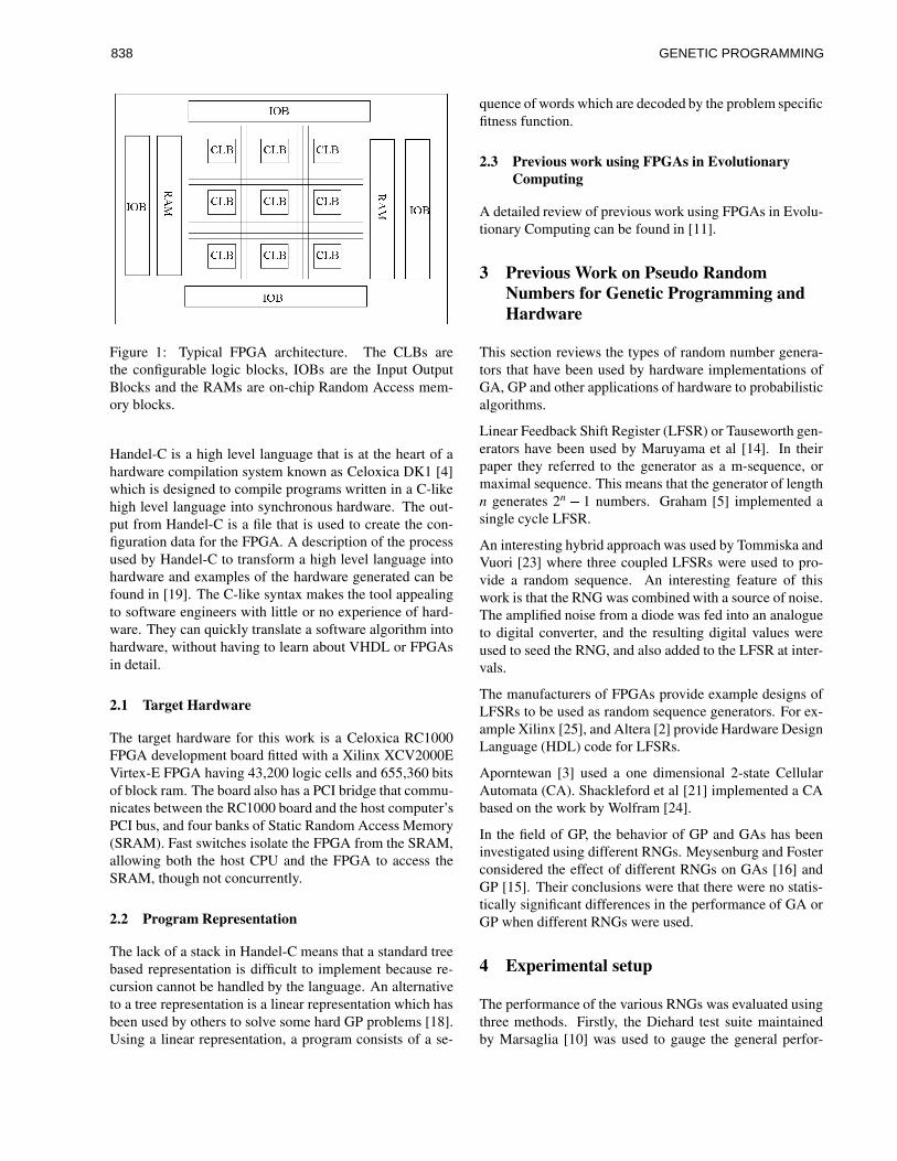
Figure 1: Typical FPGA architecture. The CLBs arethe configurable logic blocks, IOBs are the Input OutputBlocks and the RAMs are on-chip Random Access mem-ory blocks.

Handel-C is a high level language that is at the heart of ahardware compilation system known as Celoxica DK1 [4]which is designed to compile programs written in a C-likehigh level language into synchronous hardware. The out-put from Handel-C is a file that is used to create the con-figuration data for the FPGA. A description of the processused by Handel-C to transform a high level language intohardware and examples of the hardware generated can befound in [19]. The C-like syntax makes the tool appealingto software engineers with little or no experience of hard-ware. They can quickly translate a software algorithm intohardware, without having to learn about VHDL or FPGAsin detail.

2.1 Target Hardware

The target hardware for this work is a Celoxica RC1000FPGA development board fitted with a Xilinx XCV2000EVirtex-E FPGA having 43,200 logic cells and 655,360 bitsof block ram. The board also has a PCI bridge that commu-nicates between the RC1000 board and the host computer’sPCI bus, and four banks of Static Random Access Memory(SRAM). Fast switches isolate the FPGA from the SRAM,allowing both the host CPU and the FPGA to access theSRAM, though not concurrently.

2.2 Program Representation

The lack of a stack in Handel-C means that a standard treebased representation is difficult to implement because re-cursion cannot be handled by the language. An alternativeto a tree representation is a linear representation which hasbeen used by others to solve some hard GP problems [18].Using a linear representation, a program consists of a se-

quence of words which are decoded by the problem specificfitness function.

2.3 Previous work using FPGAs in EvolutionaryComputing

A detailed review of previous work using FPGAs in Evolu-tionary Computing can be found in [11].

3 Previous Work on Pseudo RandomNumbers for Genetic Programming andHardware

This section reviews the types of random number genera-tors that have been used by hardware implementations ofGA, GP and other applications of hardware to probabilisticalgorithms.

Linear Feedback Shift Register (LFSR) or Tauseworth gen-erators have been used by Maruyama et al [14]. In theirpaper they referred to the generator as a m-sequence, ormaximal sequence. This means that the generator of lengthn generates 2n

� 1 numbers. Graham [5] implemented asingle cycle LFSR.

An interesting hybrid approach was used by Tommiska andVuori [23] where three coupled LFSRs were used to pro-vide a random sequence. An interesting feature of thiswork is that the RNG was combined with a source of noise.The amplified noise from a diode was fed into an analogueto digital converter, and the resulting digital values wereused to seed the RNG, and also added to the LFSR at inter-vals.

The manufacturers of FPGAs provide example designs ofLFSRs to be used as random sequence generators. For ex-ample Xilinx [25], and Altera [2] provide Hardware DesignLanguage (HDL) code for LFSRs.

Aporntewan [3] used a one dimensional 2-state CellularAutomata (CA). Shackleford et al [21] implemented a CAbased on the work by Wolfram [24].

In the field of GP, the behavior of GP and GAs has beeninvestigated using different RNGs. Meysenburg and Fosterconsidered the effect of different RNGs on GAs [16] andGP [15]. Their conclusions were that there were no statis-tically significant differences in the performance of GA orGP when different RNGs were used.

4 Experimental setup

The performance of the various RNGs was evaluated usingthree methods. Firstly, the Diehard test suite maintainedby Marsaglia [10] was used to gauge the general perfor-


mance of the RNG. This suite consists of up to 15 tests thatare modeled on applications of random numbers. All theRNGs considered in this paper were implemented in ISO-C and were submitted to all 15 tests. The test method forDiehard is similar to that described in Meysenburg and Fos-ter [15]. Each RNG was used to generate a binary file ofabout 10 MiB2. Each Diehard test produces one or more p-values. A p-value can be considered good, bad, or suspect.Meysenburg used a scheme by Johnson [6] which assignsa score to a p-value as follows. If p� 0:998 then it is clas-sified as bad. If 0:95 � p < 0:998 then it is classified assuspect. All other p-values are classified as good. Everybad p-value scores 4, every suspect p-value scores 2 andgood p-values score zero. For each RNG, the scores foreach test were summed, and the total for each RNG is thesum of all the test scores for that RNG. Using this scheme,high scores indicate a poor RNG and low scores indicate agood RNG. The results for each test are given in AppendixA.

Each RNG was then implemented using Handel-C and usedin the hardware implementation of the artificial ant prob-lem [8][12]. In the hardware implementation the functionset differs from the standard example in only having twofunctions: F = fIF_FOOD; PROGN2gwhere IF_FOODis a two argument function that looks at the cell ahead andif it contains food it evaluates the first terminal, otherwiseit evaluates the second terminal. PROGN2 evaluates itsfirst and second terminals in sequence. The terminal setT = fLEFT; RIGHT; MOVE; NOPg, where LEFT andRIGHT change the direction the ant is facing, MOVEmoves the ant one space forwards to a new cell, and ifthe new cell contains food, the food is eaten. NOP is ano-operation terminal and has no effect on the ant but is in-cluded to make the number of terminals a power of 2, whichsimplifies the hardware logic. Each time LEFT; RIGHT orMOVE is executed, the ant consumes one time step. Therun stops when either all the time steps have been used, orthe ant has eaten all the food. All the experiments use theSanta Fe trail, which has 89 pellets of food. Each experi-ment was run 500 times and the total number of 100% cor-rect programs recorded. This is used as a measure of howwell the RNG performs. In all cases the population size is1024, the maximum program length is 31 and all experi-ments were run for 31 generations. The ant was allocated600 timesteps. The probability of selecting crossover was67%, mutation 10% and reproduction 23%. The crossoveroperator used the truncating method of limiting the maxi-mum program length, as described in [13].

Each RNG was also implemented as a stand alone appli-cation for an FPGA using Handel-C, and the number ofslices used and the maximum attainable clock frequency

2The notation MiB indicates 220 (1048576) bytes. This paperuses the binary prefixes from the NIST.[17]

was recorded. This gives a measure of the hardware re-sources needed to implement the RNG, and also an indica-tion of the logic depth required.

5 Random Number GeneratorImplementations

5.1 LFSR RNG

Figure 2 shows a schematic of the LFSR used in this work.

bit32 bit3bit4bit5bit6bit 8 .. bit30bit31 bit1bit2

Direction of shift

bit7

Figure 2: Logical Feedback Shift Register Random Num-ber Generator

The random number is read from the highest bits as re-quired. The obvious weakness of this type of RNG is thatsequential values fail the serial test described by Knuth [7,pp 55-56]. At any time step t there is a 50% probability thatthe value at time t +1 can be predicted. If for an LFSR oflength n at time t the value is v, then at time t+1 the valuewill be v=2 or v=2+2n�1. This is shown in Figure 3 wherepairs of values vt and vt+1 are plotted.

0

1e+09

2e+09

3e+09

4e+09

5e+09

0 1e+09 2e+09 3e+09 4e+09 5e+09

v(t)

v(t+1)

Figure 3: Serial test of a simple LFSR RNG

It can be seen that for any value vt there are only two pos-sible values of vt+1. Though the random number generatorruns in parallel with the main GP machine, it is possible toaccess sequential values when creating an initial program,or when choosing crossover points. There is then a possi-bility of a potentially degrading bias by using such an RNG.


5.2 Multiple LFSRs

One method of obtaining better serial test results for theLFSR of length n is to allow the LFSR to run for n cyclesbefore reading another number. Since this would limit therate at which random numbers could be generated in thepresent design it is not explored any further. However, anequivalent result can be obtained by implementing n LF-SRs of length m and using a single bit from each LFSR ateach time step. This can also be done using a single longLFSR of n�m bits, [22] effectively implementing n par-allel LFSRs. However, implementing a long shift registerin a Xilinx Virtex FPGA is not efficient because the lookup tables can implement a 16 bit shift register very easily,but longer shift registers require more extensive routing re-sources.

The effect of using a better RNG was investigated by im-plementing 32 16 bit LFSR machines that run in parallel,and initializing each LFSR to a different value. Bit32 fromeach LFSR is used to construct a 32 bit random number.The serial test result is shown in Figure 4, which showsthe serial test result for 32 LFSRs is better than the singleLFSR. This generator is referred to as the 32LFSR.

0

1e+09

2e+09

3e+09

4e+09

5e+09

0 1e+09 2e+09 3e+09 4e+09 5e+09

v(t)

v(t+1)

Figure 4: Serial test for an RNG using 32 parallel LFSRs

5.3 Cellular Automata RNG

Another popular RNG for hardware implementations isbased on Cellular Automata (CA). A one-dimensional (1D)CA consists of a string of cells. Each cell has two neighbors- left and right, or in some literature west and east respec-tively. At each time step, the value of any cell c is given by arule. For this implementation, rule 30 is used, which statesthat for any cell c at time t, ct+1 = ((westt +ct)� eastt),where� denotes the exclusive OR function. In practice theCA is implemented using a single 32 bit word, and for cell0, its right-hand neighbor is cell 31, and similarly for cell31 its left hand neighbor is cell 0. Figure 5 shows the result

of running this RNG using the serial test. As in the simpleLFSR RNG there is a distinct pattern to the numbers, butfor most values of vt there are several possible values forvt+1. This generator is referred to as 1DCA.

0

1e+09

2e+09

3e+09

4e+09

5e+09

0 1e+09 2e+09 3e+09 4e+09 5e+09

v(t)

v(t+1)

Figure 5: Serial test for a 1DCA RNG

5.4 Multiple CA generators

As in the case of the LFSR RNG, if several CAs are com-bined, the results should be much better. For this test, 32CAs were implemented, and by taking one bit from eachCA, a 32 bit random number can be generated. The serialtest appears to be much more random, as shown in Figure6. Each CA is initialized with a different pattern. This gen-erator is referred to as the 32CA

0

1e+09

2e+09

3e+09

4e+09

5e+09

0 1e+09 2e+09 3e+09 4e+09 5e+09

v(t)

v(t+1)

Figure 6: Serial test for a 32CA

5.5 Standard C RNGs

Another frequently used RNG is the linear congruential(LC) generator that is often found in implementations ofthe standard C library. The general equation for these is


I j+1 = (aIj + c) mod m, where a;c and m are constantschosen to produce a maximal length RNG. However, aspointed out by many authors (eg:[20]) these generators arenot good. Another factor against such a generator for im-plementing in hardware is that it requires one addition,one multiplication, and one modulus operator, which inHandel-C would consume a large amount of silicon andbecause of the deep logic produced, would be slow. Analternative given by [20] avoids the modulus operator, andis called the Even Quicker Generator (EQG). It is claimedthat this is about as good as any 32 bit linear congruen-tial generator. Its equation is I j+1 = aIj + c, and values fora = 1664525 and c = 1013904223 are suggested.

As a sanity check that the experimental method of rankingthe RNGs using Diehard was the same as that used by Mey-senburg, the generator known as “the mother of all gener-ators” was also implemented and run against the Diehardsuite. This is a multiply with carry generator and is de-scribed by Marsaglia [9]. It was not implemented in thehardware GP system.

5.6 Non random sequences

Until now we have considered pseudo random sequences.These are sequences where it is hard to guess the nextnumber in a sequence. As an experiment, a further set ofruns were performed with an obviously non-random num-ber generator. For this a sequential generator which gen-erates the sequence n;n+ 1;n+ 2; : : : was used. Rathersurprisingly this also worked to produce 100% correct pro-grams, though substantially fewer than the other generatorsachieved.

5.7 Truly Random Sequences

All the RNGs considered so far are not true random se-quences, relying on the manipulation of objects of finitesize, and so fail one or more of the Diehard battery oftests. So a set of random numbers was obtained from asource generated by using the atmospheric noise capturedby a radio receiver[1]. Each GP run for the ant problemneeds about half a million random numbers, so a block of10 MiB was downloaded from www.random.org, and a ran-domly selected 2 MiB block was transferred to one of theSRAM on the FPGA system using DMA. The FPGA readthis block sequentially to get its random numbers.

As reported in [23], RNGs based on sampling a source ofnoise are often slow, so they are not always applicable tohigh speed systems.

6 Experimental Results

The results from running the Diehard tests are given in Ap-pendix A and are summarized in Table 1. This shows thetotal results for each test and ranks them according to theDiehard score.

Table 1: Summary results of running the Diehard tests onthe RNGS.

RNG ScoreMother 20True 2232LFSR 162EQG 28832CA 640CA 676LFSR 756

The number of correct programs that were produced byrunning the ant problem on the hardware using each ran-dom number generator was recorded and is shown in Ta-ble 2. The results are ranked according to how many cor-rect programs were found and shows how each RNG per-formed. The table also shows the slice count for the RNGimplemented using Handel-C and the maximum clock rateas reported by the place and route tools. The slice count isa vendor and device dependent measure of the number ofFPGA logic blocks that have been used. The clock rate isan indication of the logic depth required to implement thegenerator, with deeper logic having a greater gate delay,and therefore a lower maximum clock rate. The slice countand clock rate for the true RNG assumes that the source ofrandom numbers is supplied by an external device to theFPGA, and that the FPGA simply reads the value from aport and writes it to a register.

Table 2: Summary of GP performance for all random num-ber generators tested from 500 runs of the artificial antproblem

RNG Rank Correct Slice Clockrate Fmax

(MHz)32CA 1 82 284 105True 2 81 6 >20032LFSR 3 79 130 134EQG 4 78 288 42ID CA 5 78 22 125LFSR 6 68 18 188Sequential 7 39 21 155


7 Discussion

The score obtained by the Mother RNG was close to thatobtained by Meysenburg (19), the difference being ex-plained by the fact that Meysenburg used the average of32 runs using 32 different seeds, while the work describedhere used only a single run. It is likely that using 32 dif-ferent seeds, that different scores would be observed. Thisconfirms that the experimental method used for ranking theRNGs using Diehard is comparable.

Despite the apparently serious deficiencies found in boththe simple LFSR used in the original implementation andthe simple one dimensional CA random number genera-tor, the overall effect of implementing a more sophisticatedRNG on the overall GP performance appeared to be small.This result generally agrees with the work by Meysenburgand Foster [15], with the exception that they did not con-sider a single-cycle LFSR or an obviously non-random gen-erator. The single-cycle LFSR performs the least well ofthe RNGs considered in this paper.

A surprising result was the emergence of programs when anon-random sequence was used. Clearly a non-random se-quence does not allow GP to operate as efficiently in termsof producing 100% correct programs, presumably becauseof the failure to explore some areas of the search space.

Despite the small differences in performance, from the re-sults we can say that using a different RNG from the sin-gle LFSR would improve the performance of the hardwareGP implementation by a measurable and therefore usefulamount, and that an RNG based on multiple LFSRs or mul-tiple CAs would be a better choice for a hardware GP sys-tem. The use of a truly random number source did not ap-pear to improve performance over the 1DCA, 32CA and32LFSR RNGs. This provides more evidence counteringthe notion that GP needs a very high quality RNG.

Table 2 shows that the difference in GP performance be-tween the 32CA, True, 32LFSR, EQG and 1DCA genera-tors is small. However, these 5 generators have very dif-ferent Diehard scores, so there does not appear to be astraightforward relationship between the Diehard score andthe performance of GP. This raises a question about the rolethat RNGs play in GP. Is a RNG that scores well in the stan-dard tests for randomness the best RNG for GP?

When looking at the FPGA slice counts and maximumclock rates, it is clear that the 32LFSR uses about half theFPGA resources of the 32CA, and the 32LFSR exhibits asmaller delay than the 32CA. As predicted, the EQG usesthe most FPGA resources and has very deep logic, mean-ing that it can only run at a much slower rate than the othergenerators. The EQG RNG could be re-implemented in theFPGA using pipelines to achieve a higher clock rate, but

since it performed no better than the 32CA and 32LFSR,this was not investigated any further.

Random numbers are used in several functions within a GPsystem: Initial population creation, selection and crossoverpoint selection. In common with all reported GP systems,the same RNG is been used for all these functions withina run. From a practical point of view it would appear thatthere is little point in using more than one type of RNG fordifferent functions, but from the result using a non-randomsequence a question arises about the role that random se-quences play as opposed to sequences that simply enumer-ate a set of numbers. From this it follows that differentstages in GP may use random number sequences in differ-ent ways, and that using an enumeration may be helpfulwhen investigating the dynamics of GP.

8 Conclusions

The main conclusion from this investigation is that for thehardware GP system, the simple LFSR used in the originaldesign can be improved upon by using a generator based onmultiple LFSRs, multiple CAs, or if available, a high speedsource of true random numbers. A secondary conclusionis that with the exception of the non-random sequence andthe single LFSR, there is no significant difference in GPperformance when different hardware RNGs are used.

Acknowledgments

I would like to thank Riccardo Poli for his invaluable helpin preparing this paper and the anonymous reviewers fortheir helpful comments. I would also like to thank Marconiplc, Celoxica Ltd. and Xilinx Inc. for supporting this work.

References

[1] random.org A source of true random numbers de-rived from radio noise and available on the internet.www.random.org, 2002. Last visited Jan 2 2002.

[2] Altera. Linear feedback shift register megafunction.http://www.altera.com/literature/sb/sb11_01.pdf,Dec. 2001.

[3] C. Aporntewan and P. Chongstitvatana. A Hard-ware Implementation of the compact genetic algo-rithm. IEEE Congress on Evolutionary Computation,pages 624–629, May 2001.

[4] Celoxica. Web site of Celoxica Ltd.www.celoxica.com, 2001. Vendors of Handel-C. Last visited 15/June/2001.

[5] P. Graham and B. Nelson. Genetic algorithms in soft-ware and in hardware - a performance analysis of


workstation and custom computing machine imple-mentations. In K. Pocek and J. Arnold, editors, Pro-ceedings of the Fourth IEEE Symposium of FPGAsfor Custom Computing Machines., pages 216–225,Napa Valley, Califormia, Apr. 1996. IEEE ComputerSociety Press.

[6] B. Johnson. Radix-b extensions to some commonempirical tests for pseudorandom number generators.ACM Transactions on Modelling and Computer Sim-ulation, 6(4):261–273, 1996.

[7] E. Knuth, Donald. Semi numerical algorithms, vol-ume 2. Addison-Wesley Publishing Company, 1969.

[8] J. Koza. Genetic programming: on the programmingof computers by means of natural selection. MITPress, Cambridge, MA, USA, 1992.

[9] G. Marsaglia. Yet another RNG. Posted tosci.stat.math, 1 Aug. 1994.

[10] G. Marsaglia. Web site for Diehard random numbertest suite. http://stat.fsu.edu/geo/, 2001. Last visited15/June/2001.

[11] P. Martin. A Hardware Implementation of a Ge-netic Programming System using FPGAs and Handel-C. Genetic Programming and Evolvable Machines,2(4):317–343, 2001.

[12] P. Martin. A pipelined hardware implementation ofgenetic programming using FPGAs and Handel-C. InEurogp2002, 2002.

[13] P. Martin and R. Poli. Crossover operators for a hard-ware implementation of genetic programming usingFPGAs and Handel-C. In Proceedings of the Geneticand Evolutionary Computation Conference, GECCO-2002, July 2002.

[14] T. Maruyama, T. Funatsu, M. Seki, Y. Yamaguchi,and T. Hoshino. A Field-Programmable Gate-Arraysystem for Evolutionary Computation. IPSJ Journal,40(5), 1999.

[15] M. Meysenburg and J. Foster. Random generatorquality and GP performance. In W. Banzhaf, J. Daida,A. Eiben, M. Garzon, V. Honavar, M. Jakiela, andR. Smith, editors, Proceedings of the genetic and evo-lutionary computation conference, volume 2, pages1121–1126, Orlando, Florida, USA, 13-17 July 1999.Morgan Kaufmann.

[16] M. Meysenburg and J. Foster. Randomness and GAperformance, revisited. In W. Banzhaf, J. Daida,A. Eiben, M. Garzon, V. Honavar, M. Jakiela, and

R. Smith, editors, Proceedings of the genetic and evo-lutionary computation conference, volume 1, pages425–432, Orlando, Florida, USA, 13-17 July 1999.Morgan Kaufmann.

[17] NIST. The NIST reference on constants, units anduncertainty. http://physics.nist.gov/cuu/, 2002.

[18] P. Nordin and W. Banzhaf. Evolving turing-completeprograms for a register machine with self-modifyingcode. In L. Eshelman, editor, Genetic algorithms:proceedings of the sixth international conference(ICGA95), pages 318–325, Pittsburgh, PA, USA, 15-19 July 1995. Morgan Kaufmann.

[19] I. Page. Constructing hardware-software systemsfrom a single description. Journal of VLSI Signal Pro-cessing, 1(12):87–107, Jan. 1996. Kluwer AcademicPublishers.

[20] W. Press, B. Flannery, S. Teukolsky, and W. Vetter-ling. Numerical recipes, the art of scientific comput-ing. Cambridge University Press, 1986.

[21] B. Shackleford, G. Snider, R. Carter, E. Okushi,M. Yasuda, K. Seo, and H. Yasuura. A high per-formance, pipelined, FPGA-based genetic algorithmmachine. Genetic Programming and Evolvable Ma-chines, 2(1):33–60, Mar. 2001.

[22] D. Stiliadis and A. Varma. FAST: An FPGA-basedsimulation testbed for ATM networks. Proc. ICC’96,1996.

[23] M. Tommiska and J. Vuori. Hardware implementa-tion of GA. In J. Alander, editor, Proceedings of theSecond Nordic Workshop on Genetic Algorithms andtheir Applications (2NWGA), Vaasa, Finland, 1996.

[24] S. Wolfram. Random sequence generation in cellularautomata. Adv. Appl. Math., 7:123–169, 1986.

[25] Xilinx. Pseudo random number generator.www.xilinx.com/xcell/xl35/xl35_44.pdf, Dec.2001.


Appendix A

Results of the Diehard Tests

This appendix contains the results of running the Diehard tests for all RNGs in this paper. Max score represents the casewhere an RNG fails all the tests.

Table 3: Diehard test results for all RNGs considered in this paper.Test Max

scoreLFSR EQG 32LFSR IDCA 32CA True Mother

Birthday 36 36 8 2 0 8 0 0Overlapping permutation 8 8 0 4 8 8 0 0Binary Rank 32x32 8 8 2 8 2 6 0 0Binary Rank 6x 104 104 40 8 140 70 4 6Bitstream 80 80 0 0 80 80 4 0Overlapping pairs tests 328 328 188 94 328 320 6 2Count the ones (stream) 8 8 8 8 8 8 0 0Count the ones (specific) 100 100 42 30 100 100 2 4Parking Lot 44 4 0 0 4 2 0 0Minimum Distance 4 4 0 4 4 4 0 03D spheres 84 4 0 2 4 2 4 4Squeeze 4 4 0 0 4 4 0 0Overlapping Sums 44 44 0 0 6 0 2 2Runs 16 16 0 2 16 8 0 2Craps 8 8 0 0 8 12 0 0Total 876 756 288 162 676 640 22 20


Crossover Operators for a Hardware Implementation of GP using FPGAs andHandel-C

Peter MartinDepartment of Computer Science,Essex University, Wivenhoe Park,


Riccardo PoliDepartment of Computer Science,Essex University, Wivenhoe Park,


Abstract

This paper analyses the behavior of the crossoveroperator in a hardware implementation of Ge-netic Programming using Field ProgrammableGate Arrays. Three different crossover operatorsthat limit the lengths of programs are analysed: Atruncating operator, a limiting operator that con-strains the lengths of both offspring and a limit-ing operator that only constrains the length of oneoffspring. The latter has some interesting prop-erties that suggest a new method of limiting codegrowth in the presence of fitness.

1 Introduction

Previous work has described an implementation of Ge-netic Programming using a Field Programmable Gate Ar-ray (FPGA) and a high level language to hardware com-pilation system called Handel-C [6]. This was tested us-ing the XOR and symbolic regression problems. Furtherwork described a pipelined implementation that improvedthe performance and demonstrated that the technique couldbe used to solve the artificial ant problem [7]. In both casesthe work concentrated on the implementation issues and in-creasing the clock speed of the implementation, but put toone side the study of the behavior of the system. Now thatthe raw throughput issues have been considered it is timeto look at the behavior, and investigate and analyse somealternative implementation issues.

Because of limited hardware resources in an FPGA and tokeep the design simple and therefore efficient, the maxi-mum program size is fixed. To ensure that crossover al-ways generates programs that are shorter than the maxi-mum length, the crossover operator limits the program sizeby truncating programs that exceed the maximum length.The effect of this decision is investigated in this paper andsome other alternative methods of limiting program length

are explored.

The paper begins with a brief description of the implemen-tation of a GP system using FPGAs. This is followed byan analysis of the crossover operator, with comparisons tostandard tree based GP [3]. We then consider two alter-native crossover operators and analyse their behavior. Theanalysis is then discussed and finally some further work issuggested and some conclusions are given.

2 A Hardware Implementation of GP usingFPGAs

Implementing GP in hardware is motivated by the potentialspeedups that can be obtained. The platform chosen forthis work is a Field Programmable Gate Array (FPGA). AnFPGA is a reconfigurable device than can be programmedto perform a wide range of logic functions. A typical FPGAis arranged as an array of configurable logic cells, input-output circuits and programmable interconnections, and isshown in Figure 1.

Traditionally FPGAs have been programmed using hard-ware design languages such as VHDL1, but alternative ap-proaches using high level language to hardware compila-tion techniques have also been developed, in which a highlevel imperative language is used to generate the configu-ration information for the FPGA. Handel-C [1] is one ex-ample of this technology, and has been used for the workdescribed in this paper.

For a detailed review of previous work using FPGAs inEvolutionary Computing refer to [6].

2.1 Target Hardware

The target hardware is a Celoxica RC1000 FPGA devel-opment board fitted with a Xilinx XCV2000E Virtex-E

1VHDL is a standard hardware design language. It standsfor VHSIC Hardware Design Language. VHSIC itself stands forVery High Speed Integrated Circuit.


Figure 1: Typical FPGA architecture. The CLBs arethe configurable logic blocks, IOBs are the Input OutputBlocks and the RAMs are on-chip Random Access mem-ory blocks.

FPGA having 43,200 logic cells and 655,360 bits of blockram. The board also has a PCI bridge that communicatesbetween the RC1000 board and the host computer’s PCIbus, and four banks of Static Random Access Memory(SRAM). Fast switches isolate the FPGA from the SRAM,allowing both the host CPU and the FPGA to access theSRAM, though not concurrently.

2.2 Program Representation

Handel-C does not support a stack, which means that astandard tree based representation is not straightforwardto implement because recursion is not supported by thelanguage. An alternative to a tree representation is a lin-ear representation which has been used by others to solvesome hard GP problems, for example [8]. Using a linearrepresentation, a program consists of a sequence of wordswhich are interpreted by the problem specific fitness func-tion. The hardware design uses a linear program repre-sentation with a fixed maximum size. Choosing a fixedmaximum size made the storage of programs in on-chipRAM and off-chip RAM efficient and simple to implement.Consequently a method of limiting the program size dur-ing crossover was needed. The first implementation used atruncating crossover. This is compared to a second methodof limiting lengths, called the limiting crossover operator.

3 Analysis of the crossover operator

Two separate implementations were used for the analysis.Firstly, a simple program that simulated the effects of GPcrossover was used to show the expected program lengthdistributions in the absence of fitness. We refer to this asthe GP simulator in this paper. Secondly, the hardware im-

plementation was used to obtain results both with and with-out fitness. The test problem for all the experiments wherefitness is used is the artificial ant problem.

3.1 Artificial Ant

This popular test problem was originally described by Jef-ferson [2] and in the context of GP by Koza [3]. It in-volves finding a program for an ant-like machine that en-ables it to navigate its way round a trail of food on a32x32 toroidal grid of cells within a fixed number of timesteps. In the hardware implementation the function set dif-fers from the standard example in only having two func-tions: F = fIF_FOOD; PROGN2g where IF_FOOD is atwo argument function that looks at the cell ahead and ifit contains food it evaluates the first terminal, otherwiseit evaluates the second terminal. PROGN2 evaluates itsfirst and second terminals in sequence. The terminal setT = fLEFT; RIGHT;MOVE; NOPg, where LEFT andRIGHT change the direction the ant is facing, MOVEmoves the ant one space forwards to a new cell, and ifthe new cell contains food, the food is eaten. NOP is ano-operation terminal and has no effect on the ant but is in-cluded to make the number of terminals a power of 2, whichsimplifies the hardware logic. Each time LEFT; RIGHT orMOVE is executed, the ant consumes one time step. Therun stops when either all the time steps have been used, orthe ant has eaten all the food. This test problem was chosenbecause it is known to be a hard problem for GP to solve[5].

All the results use the Santa Fe trail, which has 89 pellets offood. Each experiment was run 500 times and the mean ofall the runs taken. Unless stated otherwise, the populationsize is 1024, the maximum program length is 31 and allexperiments were run for 31 generations. The ant was allo-cated 600 timesteps. The probability of selecting crossoverwas 67%, mutation 10% and straight reproduction 23%.

3.2 Behavior Analysis

The measurement of overall GP behavior is frequently lim-ited to plotting the mean population fitness vs. genera-tion. This is shown for the artificial ant problem using thehardware implementation in Figure 2 over 500 runs. Thiswill be used as a baseline when looking at changes to theoriginal design. However, when looking for the reasonsto explain why a feature of an operator or representationhas an effect, raw performance gives us a very restrictedview of what is happening, and more analytical methodsare needed. One such method is to consider one or more as-pects of the internal population dynamics during a run. Re-cently a lot of work has been done to develop exact schematheories for Genetic Programming [10][11], which, amongother things, give us a description of the expected changes


020

4060

8010

0

0 5 10 15 20 25 30 35

Fitn

ess (

perc

ent)

Generation

Fitness value against generation

Truncating

Figure 2: GP Performance of the artificial ant problem us-ing a hardware GP system. Average of 500 runs.

in the program length distribution during a GP run. Theasymptotic distribution of program lengths is important tous because it is a way of comparing the sampling behavior(search bias) of different crossover operators and replace-ment strategies.

Starting with the GP simulator with a uniform initial lengthdistribution and ignoring the effects of fitness, Figure3 shows the expected length distribution for generations0,1,10 and 31. In this case there is no maximum programsize. This agrees with the results in [11] where the distri-bution asymptotically converges to a discrete Gamma dis-tribution.

05

1015

2025

3035

4045

50

0 5 10 15 20 25 30

Num

ber o

f Pro

gram

s

Program Length

Gen 0Gen 1

Gen 10Gen 31

Figure 3: Program length distribution for standard GPcrossover using a linear program representation, a globalreplacement strategy, non-steady state without fitness.

3.3 Truncating Crossover Operator

This crossover operator ensures programs do not exceedthe maximum program length by selecting crossover pointsin two individuals at random and exchanging the tail por-tions up to the maximum program length. Crossovers thatresult in programs exceeding the maximum length are trun-cated at the maximum length. This crossover operator wasdevised to minimize the amount of logic required and thenumber of clock cycles needed. This is illustrated in Fig-

ure 4. For two programs a and b that have lengths la and

X1=1

X2=11

I

lb

Ia'

Ib'

Len=9

Len=12

Len=2

Len=16

Crossover

a

b

a'

b'

la

Figure 4: Truncating crossover operator

lb, two crossover points xa and xb are chosen at randomso that 0 � xa < la and 0 � xb < lb. The program sizelimit is Lmax. After crossover the new lengths are l0

a =

min((xa+ lb�xb);Lmax) and l0

b =min((xb+ la�xa);Lmax).

When the GP simulator is modified to implement the trun-cating crossover, the result is shown in Figure 5 without fit-ness. The behavior of the hardware implementation using

010

2030

4050

6070

8090

0 5 10 15 20 25 30

Num

ber o

f Pro

gram

s

Program Length

Gen 0Gen 1

Gen 10Gen 31

Figure 5: Program length distribution with truncatingcrossover for standard GP without fitness.

the truncating crossover operator is shown in Figure 6. Afeature of these results is that there is initially a large peakat the maximum program size of 31, but in subsequent gen-erations the distribution tends to resemble a Gamma distri-bution like the one in Figure 3. However, it is important tonote that it is not the same Gamma distribution, because themean program length tends to decrease with this crossoveroperator. The reason is that with the truncation the amountof genetic material removed from the parents when creatingthe offspring may be bigger than the amount of genetic ma-terial replacing it. The differences between Figures 5 and6 are believed to arise because the simulator uses genera-tional GP, while the hardware implementation uses steadystate GP.

When fitness is used, the length distribution changes asshown in Figure 7, but it still retains some of the featuresof a Gamma distribution. The striking feature is the large


010

2030

4050

6070

0 5 10 15 20 25 30

Num

ber o

f Pro

gram

s

Program Length

Gen 0Gen 1

Gen 10Gen 31

Figure 6: Program length distribution using truncatingcrossover using a linear program representation without fit-ness. From the hardware implementation.

peak at the maximum program length limit which repre-sents nearly 10% of the total population.

010

2030

4050

6070

8090

100

0 5 10 15 20 25 30 35

Num

ber o

f Pro

gram

s

Program Length

Gen 0Gen 1

Gen 10Gen 31

Figure 7: Program length distribution using truncatingcrossover using a linear program representation with fit-ness. From the hardware implementation.

3.4 Limiting Crossover Operator

An alternative method of ensuring that programs do not ex-ceed the fixed limit is to repeatedly choose crossover pointsuntil both programs are below the program size limit Lmax.For two programs a and b, with lengths la and lb, twocrossover points xa and xb are chosen so that 0 � xa < laand 0 � xb < lb. After crossover the new lengths are sim-ply l0

a = xa + lb � xb and l0

b = xb + la � xa. If l0

a > Lmax

or l0

b > Lmax the selection of xa and xb is repeated untill0

a � Lmax AND l0

b � Lmax.

This is the approach taken in lilgp (versions 1.02 and 1.1)when the keep_trying parameter is enabled [12] to limitthe tree depth and the total number of nodes in a programtree during crossover. When this crossover operator is im-plemented in the GP simulator the program length distribu-tion changes, as shown in Figure 8. A feature of this resultis that the mean program length moves towards smaller val-ues. After 31 generations, the population size distribution

010

2030

4050

6070

8090

0 5 10 15 20 25 30

Num

ber o

f Pro

gram

s

Program Length

Gen 0Gen 1

Gen 10Gen 31

Figure 8: Program length distribution using limitingcrossover operator and a global replacement strategy with-out fitness.

shape resembles the one produced with standard GP.

When this method of limiting the program length was im-plemented in the hardware version, we obtained the distri-bution shown in Figure 9. In contrast to the GP simulatorthe program length distribution remains reasonably staticbetween generations 1 and 31. In an effort to understand

05

1015

2025

3035

4045

50

0 5 10 15 20 25 30

Num

ber o

f Pro

gram

s

Program Length

Gen 0Gen 1

Gen 10Gen 31

Figure 9: Program length distribution using limitingcrossover without fitness, from the hardware implementa-tion.

the different behavior between the results in Figures 8 and9 it was noted that the hardware implementation requiredboth of the offspring programs a0 AND b0 to be shorter thanLmax but that the simulation only considered one offspringat a time, effectively requiring a0 OR b0 to be shorter. Thelatter case is referred to as the single-child variant in therest of this paper, and the original the dual-child variant. Inthe case of the single-child variant, if one of the programswas larger than the maximum, it was simply discarded andthe parent substituted in its place, and if both children werelarger than the limit, the two crossover points would be cho-sen again. If both children were smaller than the limit, theywould both be available as candidates in the next gener-ation. When the hardware implementation was modifiedto incorporate the single-child variant limiting method, theresult shown in Figure 10 was obtained, closely matching


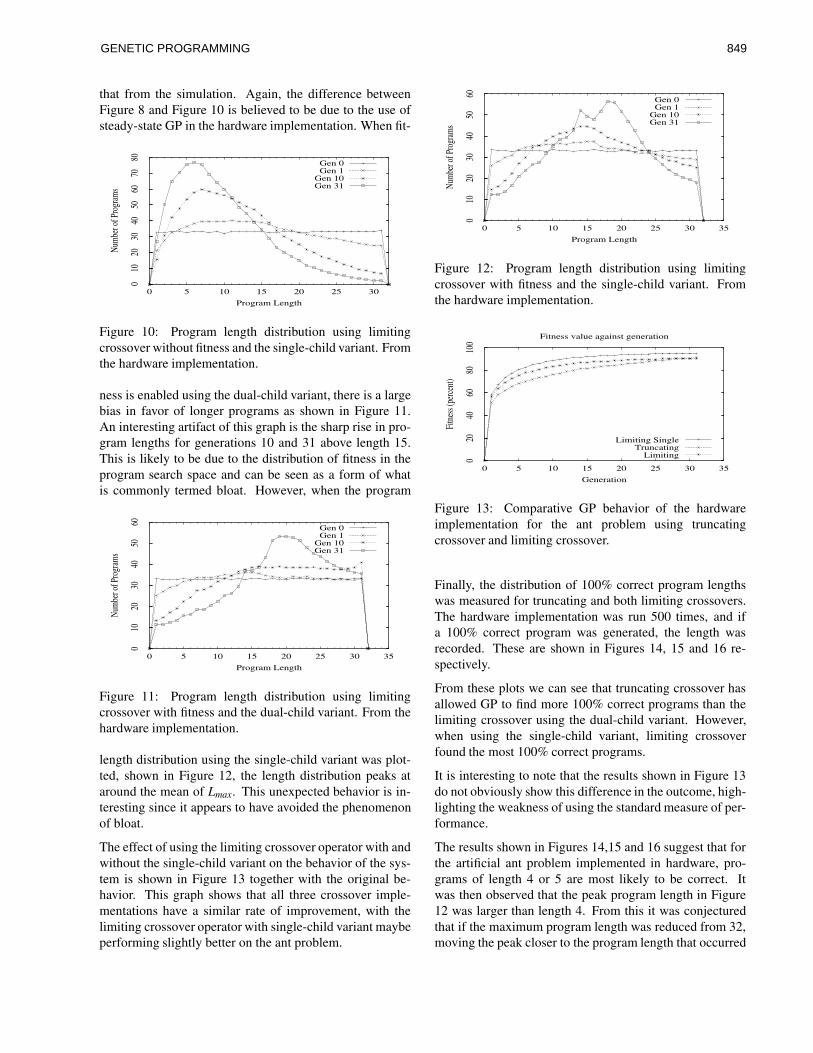
that from the simulation. Again, the difference betweenFigure 8 and Figure 10 is believed to be due to the use ofsteady-state GP in the hardware implementation. When fit-

010

2030

4050

6070

80

0 5 10 15 20 25 30

Num

ber o

f Pro

gram

s

Program Length

Gen 0Gen 1

Gen 10Gen 31

Figure 10: Program length distribution using limitingcrossover without fitness and the single-child variant. Fromthe hardware implementation.

ness is enabled using the dual-child variant, there is a largebias in favor of longer programs as shown in Figure 11.An interesting artifact of this graph is the sharp rise in pro-gram lengths for generations 10 and 31 above length 15.This is likely to be due to the distribution of fitness in theprogram search space and can be seen as a form of whatis commonly termed bloat. However, when the program

010

2030

4050

60

0 5 10 15 20 25 30 35

Num

ber o

f Pro

gram

s

Program Length

Gen 0Gen 1

Gen 10Gen 31

Figure 11: Program length distribution using limitingcrossover with fitness and the dual-child variant. From thehardware implementation.

length distribution using the single-child variant was plot-ted, shown in Figure 12, the length distribution peaks ataround the mean of Lmax. This unexpected behavior is in-teresting since it appears to have avoided the phenomenonof bloat.

The effect of using the limiting crossover operator with andwithout the single-child variant on the behavior of the sys-tem is shown in Figure 13 together with the original be-havior. This graph shows that all three crossover imple-mentations have a similar rate of improvement, with thelimiting crossover operator with single-child variant maybeperforming slightly better on the ant problem.

010

2030

4050

60

0 5 10 15 20 25 30 35

Num

ber o

f Pro

gram

s

Program Length

Gen 0Gen 1

Gen 10Gen 31

Figure 12: Program length distribution using limitingcrossover with fitness and the single-child variant. Fromthe hardware implementation.

020

4060

8010

00 5 10 15 20 25 30 35

Fitn

ess (

perc

ent)

Generation

Fitness value against generation

Limiting SingleTruncating

Limiting

Figure 13: Comparative GP behavior of the hardwareimplementation for the ant problem using truncatingcrossover and limiting crossover.

Finally, the distribution of 100% correct program lengthswas measured for truncating and both limiting crossovers.The hardware implementation was run 500 times, and ifa 100% correct program was generated, the length wasrecorded. These are shown in Figures 14, 15 and 16 re-spectively.

From these plots we can see that truncating crossover hasallowed GP to find more 100% correct programs than thelimiting crossover using the dual-child variant. However,when using the single-child variant, limiting crossoverfound the most 100% correct programs.

It is interesting to note that the results shown in Figure 13do not obviously show this difference in the outcome, high-lighting the weakness of using the standard measure of per-formance.

The results shown in Figures 14,15 and 16 suggest that forthe artificial ant problem implemented in hardware, pro-grams of length 4 or 5 are most likely to be correct. Itwas then observed that the peak program length in Figure12 was larger than length 4. From this it was conjecturedthat if the maximum program length was reduced from 32,moving the peak closer to the program length that occurred


05

1015

2025

3035

4045

50

0 5 10 15 20 25 30

Freq

uenc

y

Program Length

Lengths of 100% correct programs

68 correct programs out of 500 runs

Figure 14: Distribution of lengths of 100% correct pro-grams using the truncating crossover operator.

02

46

810

1214

0 5 10 15 20 25 30

Freq

uenc

y

Program Length



Figure 15: Distribution of lengths of 100% correct pro-grams using the dual-child variant limiting crossover op-erator.

most frequently, that GP may find even more successfulprograms. Two further experiments were therefore per-formed using maximum lengths of 16 and 8. The resultsof running the hardware implementation with these modi-fied lengths is shown in Figures 17 and 18.

This confirmed the idea that, by limiting the programlengths that GP is allowed to create, that GP producedmore 100% correct programs. The corresponding programlength distributions are shown in Figures 19 and 20. Theseboth have similar characteristics to Figure 12 and show thatthe program length distribution peaks close to the peak ofthe successful programs.

4 Discussion

The differences between the dual-child and single-childvariants can be explained by considering first the dual-child case. Starting with a uniform distribution of programlengths 0 < l � Lmax, the average program length is givenby Lavg =

Lmax2 and the average crossover point is Lavg

2 . Ev-ery crossover produces two offspring, the average lengthof which is Lmax

2 , with one smaller and one larger programproduced. When one of the offspring exceeds Lmax both

020

4060

8010

012

0

0 5 10 15 20 25 30

Freq

uenc

y

Program Length



Figure 16: Distribution of lengths of 100% correct pro-grams using the the single-child variant limiting crossoveroperator.

050

100

150

200

0 5 10 15 20 25 30

Freq

uenc

y

Program Length



Figure 17: Distribution of lengths of 100% correct pro-grams using the the single-child variant limiting crossoveroperator and a length limit of 16

crossover points are re-selected until both programs satisfythe length constraint. The result is that the average pro-gram length using this crossover will remain Lmax

2 . How-ever, in the single-child case, only one child needs to meetthe length constraint. With one long and one short off-spring, the short offspring will be more likely to satisfy theconstraint and so be selected for propagation. Because theshorter program is preferred, the mean program length willtend to continually decrease. In summary, in the absenceof fitness, the single-child variant selects programs that areon average smaller than Lmax

2 . In the presence of fitnesswe believe that this pressure to decrease the mean programlength competes with the well documented tendency of GPprograms to grow in the presence of fitness. The result isthat when using the single length constraint and an upperbound on the program length, the program length distribu-tion does not have a strong bias to longer lengths.

A side effect of using the single child variant is that when along program is rejected, a copy of the parent is propagatedto the next generation. This means that even if crossover isused as the only operator, a proportion of straightforwardreproduction will be present.


050

1001

5020

0250

3003

5040

0450

0 5 10 15 20 25 30

Freq

uenc

y

Program Length



Figure 18: Distribution of lengths of 100% correct pro-grams using the the single-child variant limiting crossoveroperator and a length limit of 8

020

4060

8010

012

0

0 2 4 6 8 10 12 14 16

Num

ber o

f Pro

gram

s

Program Length

Gen 0Gen 1

Gen 10Gen 31

Figure 19: Program length distribution using limitingcrossover with fitness and the single-child variant. Maxi-mum length limited to 16. From the hardware implementa-tion.

A practical penalty of the limiting crossover approachis that multiple passes may be required to obtain twocrossover points that satisfy the length constraints. De-pending on the implementation this could have an impacton the time needed to complete a GP run. In practice formost problems the time required for crossover in a stan-dard GP system is much smaller than the time for evaluat-ing programs, and so will only extend the time required bya small factor. In the hardware implementation, crossoveris performed in parallel with evaluation, so there will beno impact for most problems where fitness evaluation takeslonger than selection and breeding. For the artificial antproblem implemented in hardware, the limiting crossoveroperators did not have any effect on the overall perfor-mance of the design, both the clock speed and number ofclock cycles remained the same as the truncating crossoverimplementation. It is worth noting that the single-child lim-iting crossover will need fewer iterations to find a legal off-spring, so this will have a smaller effect on the overall per-formance.

The effect of adjusting the program length limit so that thepeak in the length distribution is closer to the peak of opti-

050

100

150

200

250

300

350

0 1 2 3 4 5 6 7 8

Num

ber o

f Pro

gram

s

Program Length

Gen 0Gen 1

Gen 10Gen 31

Figure 20: Program length distribution using limitingcrossover with fitness and the single-child variant. Maxi-mum length limited to 8. From the hardware implementa-tion.

mal program lengths suggests that allowing programs to beunlimited in length may be detrimental to using GP effec-tively.

5 Further work

From the results in [10] we would expect similar behaviorwhen these techniques are applied to standard tree basedGP, and this is currently being investigated.

Other techniques have been suggested for controlling theprogram size during evolution, such as the smooth oper-ators [9], homologous and size fair operators [4] whichcould also be adapted to a hardware implementation.

So far, only one problem has been analysed using the hard-ware implementation of GP and to get a more completepicture of the effects of the design decisions more problemsneed to be implemented and analysed.

6 Conclusions

This analysis, based on measuring the program length dis-tributions was prompted by the results from the work ona general schema theory of GP. It has led us to an imple-mentation of crossover that allows us to constrain the max-imum program lengths. For the ant problem implementedin hardware we have discovered a mechanism that avoidsthe effects of unconstrained program growth, and indeedallows us to obtain more correct programs.

In conclusion, all three crossover operators are effectivein the hardware implementation when applied to the arti-ficial ant problem, with the single-child limiting crossoverperforming ahead of the other two. The behavior of thesingle-child limiting crossover in the presence of fitness isinteresting and suggests another mechanism for controllingcode growth.


Acknowledgments

We would like to thank the anonymous reviewers for theirhelpful comments. The first author would like to thankMarconi plc, Celoxica Ltd. and Xilinx Inc. for support-ing this work.

References

[1] Celoxica. Web site of Celoxica Ltd.www.celoxica.com, 2001. Vendors of Handel-C. Last visited 15/June/2001.

[2] D. Jefferson, R. Collins, C. Cooper, M. Dyer,M. Flowers, R. Karf, C. Taylor, and A. Wang. Evolu-tion as a theme in artificial life: The Genesys/Trackersystem. In C. Langton, editor, Artificial Life II.Addison-Wesley Publishing Company Inc., 1992.

[3] J. Koza. Genetic programming: on the programmingof computers by means of natural selection. MITPress, Cambridge, MA, USA, 1992.

[4] W. Langdon. Size fair and homologous tree geneticprogramming crossovers. In W. Banzhaf, J. Daida,A. Eiben, M. Garzon, V. Honavar, M. Jakiela, andR. Smith, editors, Proceedings of the genetic and evo-lutionary computation conference, volume 2, pages1092–1097, Orlando, Florida, USA, 13-17 July 1999.Morgan Kaufmann.

[5] W. Langdon and R. Poli. Why ants are hard.In J. Koza, W. Banzhaf, K. Chellapilla, K. Deb,M. Dorigo, D. Fogel, M. Garzon, D. Goldberg, H. Iba,and R. Riolo, editors, Genetic programming 1998:proceedings of the third annual conference, pages193–201, University of Wisconsin, Madison, Wiscon-sin, USA, 22-25 July 1998. Morgan Kaufmann.

[6] P. Martin. A Hardware Implementation of a Ge-netic Programming System using FPGAs and Handel-C. Genetic Programming and Evolvable Machines,2(4):317–343, 2001.

[7] P. Martin. A pipelined hardware implementation ofgenetic programming using FPGAs and Handel-C. InEurogp2002, 2002.

[8] P. Nordin and W. Banzhaf. Evolving turing-completeprograms for a register machine with self-modifyingcode. In L. Eshelman, editor, Genetic algorithms:proceedings of the sixth international conference(ICGA95), pages 318–325, Pittsburgh, PA, USA, 15-19 July 1995. Morgan Kaufmann.

[9] J. Page, R. Poli, and W. Langdon. Smooth uniformcrossover with smooth point mutation in genetic pro-gramming: A preliminary study. In R. Poli, P. Nordin,W. Langdon, and T. Fogarty, editors, Genetic pro-gramming, proceedings of EuroGP’99, volume 1598of LNCS, pages 39–49, Goteborg, Sweden, 26-27May 1999. Springer-Verlag.

[10] R. Poli. General schema theory for genetic program-ming with subtree-swapping crossover. In J. Miller,M. Tomassini, P. Lanz, C. Ryan, G. Andrea, B. Tet-tamanzi, and W. Langdon, editors, Genetic Program-ming, Proceedings of EuroGP’2001, volume 2038 ofLNCS, pages 143–159, Lake Como, Italy, Apr. 2001.EvoNET, Springer-Verlag.

[11] R. Poli and N. F. McPhee. Exact schema theoremsfor GP with one-point and standard crossover op-erating on linear structures and their application tothe study of the evolution of size. In J. F. Miller,M. Tomassini, P. L. Lanzi, C. Ryan, A. G. B. Tetta-manzi, and W. B. Langdon, editors, Genetic Program-ming, Proceedings of EuroGP’2001, volume 2038 ofLNCS, pages 126–142, Lake Como, Italy, 18-20 Apr.2001. Springer-Verlag.

[12] D. Zongker and B. Punch. Lilgp 1.01 user’s manual.Technical report, Michigan State University, USA, 26Mar. 1996.


Using schema theory to explore interactions of multiple operators

Nicholas Freitag McPheeDivision of Science and MathematicsUniversity of Minnesota, Morris, USA

[email protected]

Riccardo PoliDepartment of Computer Science

University of Essex, [email protected]+44-1206-872338

Abstract

In the last two years the schema theory for Ge-netic Programming (GP) has been applied to theproblem of understanding the length biases of avariety of crossover and mutation operators onvariable length linear structures. In these initialpapers, operators were studied in isolation. Inpractice, however, they are typically used in var-ious combinations, and in this paper we presentthe first schema theory analysis of the complexinteractions of multiple operators. In particular,we apply the schema theory to the use of standardsubtree crossover, full mutation, and grow muta-tion (in varying proportions) to variable lengthlinear structures in the one-then-zeros problem.We then show how the results can be used toguide choices about the relative proportion ofthese operators in order to achieve certain struc-tural goals during a run.

1 Introduction

Most (if not all) Genetic Programming (GP) operators havea variety of biases with respect to both the syntax and thesemantics of the trees they produce. These biases can workagainst or in favor of the biases implied by the fitness func-tion, which makes understanding these biases crucial to un-derstanding the behavior of and relationships among thevarious operators.

These interactions can be quite complex, however, and con-sequently understanding them can be difficult. While thereis a considerable literature examining the interactions ofmutation and crossover in areas like Genetic Algorithms(GAs), there is much less reported work on the interactionsof operators in GP. Notable exceptions include the workof O’Reilly [10], Banzhaf, et al [1], and Luke and Spec-tor [5, 6, 4]. These studies are primarily experimental in

nature, and all suggest that understanding operator interac-tions is difficult. It would thus be useful to have a theoreti-cal approach to these problems that might allow us to betterunderstand operator interactions, and choose combinationsof operators in a more principled manner.

In the last few years work on schema theory for GP hasmade huge progress, generating not only an exact the-ory, but also one applicable to a variety of operators usedin practice, including: one-point crossover [12, 14, 11,13], standard and other subtree-swapping crossovers [14,16, 7], different types of subtree mutation and headlesschicken crossover [15, 8], and the class of homologouscrossovers [17].

In [16, 7] we showed how these recent developments in GPschema theory can be used to better understand the biasesinduced by the standard subtree crossover when geneticprogramming is applied to variable length linear structures.In particular we showed that subtree crossover has a verystrong bias towards oversampling shorter strings and, insome senses, works against bloat. In [15, 8] we derived ex-act schema equations for subtree mutation on linear struc-tures, using both the full and grow methods to generate thenew, random subtrees. Iterating those equations on both aflat fitness landscape and a needle-in-a-haystack style prob-lem, called the one-then-zeros problem, we showed thatboth of these subtree mutation operators have strong biaseswith regard to the population’s length distribution. Similarto the bias of subtree crossover, we found that these muta-tion operators are strongly biased in favor of shorter stringsin both these fitness domains.

In this paper we combine the schema theory for differentoperators and apply them to the problem of better under-standing the behavior produced by their interaction. Study-ing these complex interactions is particularly easy usingthe schema formalization because we can simply use aweighted sum of the schema equations generated for eachoperator in isolation. We also show how the theory can beused to design competent GP systems by guiding the choice


of combinations of operators together with their parametersettings.

The work reported here is all on GP with linear structures(not unlike those used in, e.g., [9, 2]), although the schematheory on which it is based is much more general. We havechosen in these applications to focus on linear structuresbecause the theoretical analysis is more manageable andthe computations are more tractable. This has yielded anumber of important results for the linear case, and prelim-inary results further suggest that many of the key ideas hereare also applicable (at least in broad terms) to the non-lineartree structures typically used in GP.

In Sec. 2 we will introduce the schema theorem for GP us-ing linear structures, standard crossover and mutation, andwe will show how easily the theory for different operatorscan be combined. We then apply the theory in Sec. 3 tothe one-then-zeros problem and use the theory to both pre-dict and better understand the changes in the distribution offit individuals and of sizes (Sec. 4). We finish with someconclusions and ideas for future research (Sec. 5).

2 Schema theory for GP on linear structures

2.1 Operators

In this paper we will consider three common GP operators:the standard subtree-swapping GP crossover operator, andthe full and grow mutation operators. Each operator acts byremoving a non-empty suffix of an individual and replacingit with a new suffix, with the production of that suffix beingthe primary difference between the operators.

More formally, in a linear-structure GP where F is theset of non-terminal nodes and T is the set of terminalnodes, individuals can be seen as sequences of symbolsc0c1 : : : cN�1 where ci 2 F for i < N � 1 and cN�1 2 T .Each of the operators, then, starts by removing a non-emptysuffix cjcj+1 : : : cN�1 (where j is chosen uniformly suchthat 0 � j < N ) and replacing it with a new non-emptystring.1

In the case of crossover, the new string is taken to be asuffix dj0dj0+1 : : : dN 0

�1 of another parent d0d1 : : : dN 0�1,

where j0 (which could differ from j) is chosen uniformlysuch that 0 � j

0< N

0.

1The requirement that suffixes be non-empty while prefixesare allowed to be empty comes from standard practice in GP. Itdoes, however, create a number of mild but annoying asymmetrieswhich often clutter up the analysis (see, e.g., [18]).

Both full and grow mutation generate the new suffix ran-domly, and they differ in how the new random subse-quences are generated, and in particular how their sizes aredetermined. In full mutation, the subsequence has a spec-ified length D; thus non-terminals are selected uniformlyfrom F until length D � 1 is reached, at which point a ter-minal is selected uniformly from T . In grow mutation, onthe other hand, one chooses from the set of all functionsand terminals every time, only terminating the creation ofthe subsequence when a terminal is chosen; thus for growmutation there is no a priori limit on the size of the result-ing sequences.

2.2 Schema theory definitions

In this section we will present a series of crucial definitionsthat allow us to represent schemata, and count and buildinstances of schemata.

Just as we defined a linear GP structure to be a sequenceof symbols, we will also define a linear GP schema asthe same kind of sequence c0c1 : : : cN�1 except that a new“don’t care” symbol ‘=’ is added to both F and T .2 Thusschemata represent sets of linear structures, where the po-sitions labelled ‘=’ can be filled in by any element of F (orT if it is the terminal position). A few examples of schemaare:3

� (=)N : The set of all sequences of length N .

� 1(=)a: The set of all sequences of length a+1 startingwith a 1.

� 1(0)a: The singleton set containing the symbol 1 fol-lowed by a 0’s.

Now that we can represent schemata, we present a series ofdefinitions that allow us to count instances of schemata.

Definition 1 (Proportion in population) �(H; t) is theproportion of strings in the population at time t matchingschema H . For finite populations of size M , �(H; t) =

m(H; t)=M , where m(H; t) is the number of instances ofH at time t.

Definition 2 (Selection probability) p(H; t) is the proba-bility of selecting an instance of schema H from the pop-ulation at time t. This is typically a function of �(H; t),the fitness distribution in the population, and the details

2This new ‘=’ symbol plays a role similar to that of the ‘#’“don’t care” symbol in GA schema theory. For historical reasons,however, ‘#’ has been assigned another meaning in the more gen-eral version of the GP schema theory [14].

3We will use the superscript notation from theory of computa-tion, where xn indicates a sequence of n x’s.


of the selection operators. With fitness proportionate se-lection, for example, p(H; t) = �(H; t) � f(H; t)=f(t),where f(H; t) is the average fitness of all the instances ofH in the population at time t and f(t) is the average fitnessin the population at time t.

Definition 3 (Transmission probability) �(H; t) is theprobability that an instance of the schema H will be con-structed in the process of creating a new individual for thepopulation at time t+1 out of the population at time t. Thiswill typically be a function of p(K; t), the various schemataK that could play a role in constructing H , and the detailsof the various recombination and mutation operators beingused.

Definition 4 (Creation probability) �mut(H; t) is theprobability that some GP subtree mutation operator willgenerate a new, random subtree that is an element of theschema H in generation t.

To clarify which operator we are working with, we in-troduce specialized forms of the transmission probabilityfunction �, namely �xo for the transmission probability duespecifically to crossover, �FULL for the transmission prob-ability due specifically to subtree mutation using the fullmethod, and �GROW for the transmission probability duespecifically to subtree mutation using the grow method.

We can now model the standard evolutionary algorithm asthe transformation

�(H; t)select�! p(H; t)

mutateXO�! �(H; t)

sample�! �(H; t+ 1):

Here the arrows indicate that some new distribution (onthe RHS of the arrow) is generated by applying the speci-fied operation(s) to the previous distribution (on the LHS).So, for example, the process of selection can be seen as atransformation from the distribution of schemata �(H; t) tothe selection probability p(H; t). A crucial observation isthat, for an infinite population, �(H; t + 1) = �(H; t) fort � 0, which means we can iterate these transformationsto exactly model the behavior of an infinite population overtime.

To formalize the creation of instances of a linear schemaH = c0c1 : : : cN�1 we define

u(H; i; k) = c0c1 : : : ci�1(=)k�i

l(H; i; n) = (=)n�N+icici+1 : : : cN�1

Here u(H; i; k) is the schema of length k matching the left-most i symbols of H , and l(H; i; n) is the schema of lengthnmatching the rightmostN�i symbols ofH .4 The impor-tant property of u and l is that if one uses standard crossover

4u and l are based on operators U and L (see, e.g., [14])

which match the upper and lower parts of general, non-linear, GPschemata.

to crossover any instance of u(H; i; k) at position i withany instance of l(H; i; n) at position n � N + i, the re-sult will be an instance of H , provided5

k + n > N , and0 " (N � n) � i < N # k. Further, these are the onlyways to use standard crossover to construct instances ofH ,so these definitions fully characterize the mechanism forconstructing instances of H .

2.3 The schema theorem

[7, 8] provide schema theorems for each of our three opera-tors when used in isolation. Here we extend these results tothe case where all three operators can be used in the samerun, each with specified proportions. Since we use exactlyone operator to generate any given individual, the probabil-ity that we construct an instance of a schema (i.e., �(H; t))is simply the sum of the probabilities of each specific op-erator constructing such an instance, each weighted by thelikelihood of choosing that operator. This leads to the fol-lowing:

Theorem 1 (Schema theorem for combined operators)For GP on linear structures using standard crossover withprobability pxo, full mutation with length D and probabilitypFULL, and grow mutation with probability pGROW, such thatpxo + pFULL + pGROW = 1, we have

�(H; t) = pxo � �xo(H; t)

+ pFULL � �FULL(H; t) + pGROW � �GROW(H; t)

where

�xo(H; t) =Xk>0n>0

k+n>N

� 1

k � n

�X

0"(N�n)�i<N#k

p(u(H; i; k); t)

�p(l(H; i; n); t)�;

�FULL(H; t) =Xk>0

0�i<N#k

�1

k� p(u(H; i; k); t)

� �FULL(cici+1 : : : cN�1)

�

�GROW(H; t) =Xk>0

0�i<N#k

�1

k� p(u(H; i; k); t)

� �GROW(cici+1 : : : cN�1)

�;

and q = jFj=(jFj+ jT j).

5We will use " as a binary infix max operator, and # as a binaryinfix min operator.


Due to space restrictions we simply report the general ex-pressions for the quantities �xo, �FULL, and �GROW for thelinear case without providing any proofs. The interestedreader can find these, together with extensive characteriza-tions of the behavior of crossover and mutation when usedseparately, in [7, 8].

3 The one-then-zeros problem

We will now apply the Schema Theorem to the one-then-zeros problem. We will start by defining and motivating theproblem, and then show how the schema theorem can beused to better understand the effects of multiple operatorinteraction on this problem.

3.1 One-then-zeros problem definition

In this problem we have F = f0; 1g and T = f0g, whereboth 0 and 1 are unary operators. This gives us a prob-lem that is essentially equivalent to studying variable lengthstrings of 0’s and 1’s, with the constraint that the stringsalways end in a 0. Fitness in this problem will be 1 if thestring starts with a 1 and has zeros elsewhere, i.e., the stringhas the form 1(0)a where a > 0; fitness will be 0 otherwise.

One of the reasons for studying this problem is that un-der selection and crossover this problem induces bloat [7],whereas this does not happen when using the full and growmutation operators [8]. The key advantage of this prob-lem is that in order to fully and exactly describe the length-evolution dynamics and the changes in solution frequencyof infinite populations, it is necessary to keep track of onlytwo classes of schemata: those of the form (=)N and thoseof the form 1(0)a. Unfortunately most problems are not sorestricted, and one is typically forced to track the propor-tion of many (possibly intractably many) more schemata.

3.2 Analyzing one-then-zeros

To apply the schema theorem to the one-then-zeros prob-lem one needs to calculate the probabilities �xo, �FULL, and�GROW for both of the schema (=)N and 1(0)a, and theprobabilities �FULL and �GROW for both of the schema 1(0)a

and (0)a. These can be calculated from the equations re-ported above and are also provided in explicit form in [7, 8],so we will not re-derive these results here.

If we assume an infinite population, we can numericallyiterate the equations in the Schema Theorem to better un-derstand the behavior of an infinite GP population on thisproblem. Tracking these distributions over time becomesexpensive in terms of computational effort.6 A crucial

6We have found, though, that ignoring values of � below somesmall threshold (we have used 10

�10) seems to have little impact

0

0.05

0.1

0.15

0.2

0.25

0 5 10 15 20 25 30 35 40

Pro

port

ion

in p

opul

atio

n

Length

Final distributions for operators in isolation

Grow mutationFull mutation

Crossover

Figure 1: The distributions of lengths after 50 generations whenusing the three recombination operators individually on the one-then-zeros problem. The tail of the crossover distribution contin-ues past the right hand side of the graph, with lengths above 300still having proportions above 10�10 .

point, though, is that these equations only need to be runonce, and have no stochastic effects. They are exact cal-culations of the relevant quantities (up to the limitationsof the floating point representation), and once computedneed never be computed again. This is in contrast to typicalempirical results in evolutionary computation, where com-binations of large populations and multiple runs are nec-essary to smooth out the stochastic effects, and even thenthere is no guarantee that any two sets of runs will havesimilar behavior.

4 One-then-zeros results

We know (see, e.g., [7, 16, 8, 15]) that each of these op-erators has significant biases when used on its own, andFig. 1 summarizes some of the earlier results by presentingthe final length distributions for each of the operators whenacting alone on the one-then-zeros problem. This makes itclear that the three operators all have very different lengthbiases, which suggests that they may indeed demonstrateinteresting behaviors when used in combination.

We can now iterate this new combined schema equation tostudy these combined interactions and their biases, and touse such results to guide the choices of the proportions ofoperators to help satisfy a variety of goals. As an examplein this paper we will consider the following goals:

1. Avoid both bloating and shrinking, by having the av-erage size after 50 generations be as close as possibleto the initial average size.

on the numeric results and can greatly speed up the calculationssince it significantly slows the growth of the number of stringsthat need to be tracked.


2. Avoid both bloating and shrinking (as above), but alsomaximize the number of correct individuals.

3. Maximize the proportion of small solutions (as op-posed to just short strings).

4. Reach a state where the proportion of 1(0)30 exceeds0.01 as early as possible.

In all these simulations we will be applying the three oper-ators discussed earlier (standard subtree crossover, full mu-tation, and grow mutation) on the one-then-zeros problem.A depth limitD = 5will be used for full mutation. Our ini-tial population will consist of equal proportions (10% each)of the strings 1(0)i for 1 � i � 10; thus the average lengthin the initial population is 6.5.

To study the interaction of the operators, the schema equa-tions from Theorem 1 were iterated 66 different times, us-ing each of the legal combinations of proportions of (stan-dard) crossover, grow mutation, and full mutation with val-ues from the set f0; 0:1; 0:2; 0:3; : : : ; 0:9; 1g. We’ll usetriples of the form (pxo; pFULL; pGROW) to indicate a combi-nation of parameter settings where the first is always theproportion of crossover, the second the proportion of fullmutation, and the third the proportion of grow mutation.

4.1 General observations

While the majority of these iterations had converged after50 generations, there were several which had not. Thesewere typically those with sufficiently high crossover prob-abilities that bloat was occurring and the average lengthswere clearly still growing after 50 generations. As an ex-ample, the configuration (0.8, 0, 0.2) has an average lengthof 7.98 after 50 generations, and is thus not a terrible so-lution to the problem of avoiding bloat and shrinkage asdefined in Sec. 4.2 below. It seems highly likely, how-ever, that if we were to continue iterating the equations withthese parameters for another 100 generations we would gethigher average length, thereby doing a worse job of meet-ing the goal of avoiding bloat and shrinkage. This isn’tnecessarily a concern, however, since actual GP runs al-ways have a finite number of generations. Thus if we knowwe’re likely to run our GP for 100 generations, we can it-erate these schema equations and try to find settings thatmeet our goals (whatever they happen to be) at the end of100 generations regardless of whether further generationswould take us away from our goals.

It should also be noted that the initial uniform distributionof lengths is very unstable in the sense that any combina-tion of operators will generate a very different distributionimmediately in the first generation. As an example, thesettings (0.1, 0.7, 0.2) have an average length after 50 gen-erations that’s very close to the average length in the initial

distribution (6.5). The distribution itself (shown in Fig. 3)is far from uniform, however. This seems to be a generalproperty of “interesting” operators, namely that they have afavored length distribution that they move to quite quickly,and while fitness can modify that tendency, it rarely elimi-nates it entirely.

4.2 Avoid bloat and shrinkage

In our first example the goal will be to avoid both bloat-ing and shrinkage by searching for a collection of operatorprobabilities such that the average length after 50 genera-tions is as close as possible to the initial average size.

Out of our 66 configurations, five had a final average fitnessthat was less than 0.15 away from the initial average of 6.5(see Table 1); the next closest combination of parametersettings had an absolute difference of over 0.23. Note thatin each case the proportion of grow mutation was 0.2. Infact the 20 configurations whose final average lengths wereclosest to 6.5 all had small non-zero proportions for growmutation (between 0.1 and 0.4); at the same time, however,those 20 configurations had a broad range of full mutationproportions (ranging from 0 to 0.9) and crossover propor-tions (from 0 to 0.8). Those combinations where the pro-portion of crossover was over 0.5, however, all had averagelengths that were still climbing after 50 generations, so it’slikely that they would continue to diverge from 6.5 if weiterated the equations for more generations. Thus the cru-cial factors for long-term size stability in this problem seemto be a small non-zero proportion of grow, and a crossoverproportion of at most 0.5 so the sizes don’t bloat above 6.5.

Most (but not all) of the configurations where the pro-portion of grow was 0.2 had final average lengths closeto 6.5; the smallest average length after 50 generationswas 6.36 (for (0:4; 0:4; 0:2)), and the largest was 7.98 (for(0:8; 0; 0:2)). As discussed above, however, those parame-ter sets with higher crossover proportions probably hadn’tconverged after just 50 generations, and their final averageswould likely continue to grow if we iterated more genera-tions. Taking that into account the range of final averagelengths is quite small, being from 6.35 to 6.46 when theproportion of grow is 0.2 and the proportion of crossover isat most 0.5.

Looking at Fig. 2, we can see that in each of these casesthere was an initial jump away from 6.5 (caused by the in-stability of the initial uniform length distribution), followedby a fairly rapid convergence to an average value close to6.5. The slowest to converge was the case where we had50% crossover, and that curve in fact looks similar to thebloating seen in [7], with an asymptote close to 6.5.

Fig. 3 shows the final distribution of lengths for each ofthese five parameter settings. While each of these distribu-


XO Full Grow Diff. from 6.5 Prop. fit0.1 0.7 0.2 0.081 0.190.2 0.6 0.2 -0.045 0.260.3 0.5 0.2 -0.131 0.310.4 0.4 0.2 -0.147 0.370.5 0.3 0.2 -0.045 0.43

Table 1: Parameter settings for the five configurations that cameclosest to having the same average length after 50 generations asthe average length of the initial distribution. “XO” is the pro-portion of crossover, and “Full” and “Grow” are the proportionsof full and grow mutation. “Diff. from 6.5” is the difference be-tween the actual final average length for this set of parameters andthe initial average length (6.5); negative values mean that the finalaverage length was less than 6.5. “Prop. of fit” is the proportionof the individuals produced in the last generation that were fit.

5.6

5.8

6

6.2

6.4

6.6

6.8

0 5 10 15 20 25 30 35 40 45 50

Ave

rage

leng

th

Generation

Avg length over time near 6.5

(0.1,0.7,0.2)(0.2,0.6,0.2)(0.3,0.5,0.2)(0.4,0.4,0.2)(0.5,0.3,0.2)

6.5

Figure 2: Average lengths over time for the five collections ofparameter settings leading to a final average length closest to theinitial average length (6.5).

tions has an average length that is nearly equal to that ofthe initial uniform distributions, none of these distributionsis remotely uniform. They instead exhibit combinations offeatures seen in earlier studies of using single recombina-tion operators on this problem (see Fig. 1). In each case,for example, we see a peak at length=5 which is due to fullmutation with depth 5, and the height of the peak is clearlycorrelated to the full mutation probability.

4.3 Avoid bloat and shrinkage, maximizing correctproportion

In the preceding example we looked for parameter settingsthat avoided both bloat and shrinkage. It’s possible, how-ever, that this goal was met at the expense of correctness. Agiven collection of parameter settings could, for example,generate the desired average size, but have a very low pro-portion of fit individuals. This would in turn greatly reducethe effective population size since most of the generatedindividuals can never be selected for recombination.

0

0.05

0.1

0.15

0.2

2 4 6 8 10 12 14 16 18 20

Pro

port

ion

in p

opul

atio

n

Length

Final distributions with average length 6.5

(0.1, 0.7, 0.2)(0.2, 0.6, 0.2)(0.3, 0.5, 0.2)(0.4, 0.4, 0.2)(0.5, 0.3, 0.2)

Figure 3: Final length distributions of the five parameter settingswhose final average length was closest to the initial average length(6.5).

We can assess this by looking at the proportion of correctindividuals in the final generation for each set of parametervalues, and we indeed see that there are substantial differ-ences among these five configurations (see Table 1), withthe values ranging from 0.19 to 0.43. It’s also clear thatincreased probabilities of crossover correspond with in-creased proportion of fit individuals. This is not surprisingsince increased probabilities of crossover also correspondto decreased probabilities of full mutation, and full muta-tion is rarely going to produce a fit offspring in this prob-lem [8]. Crossover on the other hand, has a high probabilityof generating correct offspring, especially when given twocorrect, fairly long individuals as parents [7].

Another approach to optimizing these two criteria wouldbe to start by identifying the configurations with high pro-portion of fit individuals in the final generation, and thenchoosing from those the parameter settings that also lead tofinal average lengths near 6.5. The settings with the highestproportion of fit individuals are those with high crossoverprobabilities, but these configurations also have the highestfinal average lengths (because high crossover probabilitieslead to bloat in this problem [7]). One of the best settingsis (0.8, 0.0, 0.2), which has a final average length of 7.98(nearly 1.5 nodes longer than the original average of 6.5)but a final proportion of fit individuals of 0.65 (about 0.22higher than the proportion generated by (0.5, 0.3, 0.2)).

4.4 Maximize proportion of small solutions

Now consider the case where we want to minimize the av-erage size of the fit individuals (i.e., those of the form 1(0)a

for a > 0). There are quite a few combinations of param-eter settings that lead to average size of fit individuals thatare just above 3. The three smallest are (0, 0, 1), (0.1, 0,0.9), and (0.2, 0, 0.8) with final average sizes of fit individu-


als 3.02, 3.04, and 3.07 respectively. This suggests that (forthis problem) the best way to make short correct solutionsis to primarily use grow mutation, with small amounts ofcrossover being acceptable as well. Adding small amountsof full mutation doesn’t lead to much bigger average sizes(the average size for (0, 0.1, 0.9), for example, is 3.13) de-spite the fact that depth mutation always generates stringsof length at least 1+D (or 6 in our case). This is probablydue to the fact that full mutation will very rarely generatecorrect individuals in this problem.

If one wanted to further maximize the proportion of fit in-dividuals, then the three candidate combinations have pro-gressively increasing proportion of fit individuals; the high-est is (0.2, 0, 0.8), which has a proportion of 0.41. If welook more broadly, we find that (0.6, 0, 0.4) has a some-what higher proportion of fit individuals after 50 genera-tions (0.49), with the average size of fit individuals beingonly slightly higher (3.54).

4.5 Find solutions of length 31 quickly

For our final example we will consider the goal of find-ing solutions of the form 1(0)30 as quickly as possible.There are a variety of motivations for this sort of goal,but one might be that instead of only having a two levelfitness function, we might have a three level fitness func-tion: Fitness 0 for individuals that don’t have the “one thenzeros” pattern, fitness 1 for individuals of the form 1(0)a,a 6= 30, and fitness 2 for individuals of the form 1(0)30. Ifwe further assume that our run will terminate as soon as wediscover a target individual 1(0)30, then dynamics of sucha run are identical to the original one-then-zeros problem,except they terminate upon discovery of a target individual.

Thus we can use our schema theory results to discover whatparameter settings lead most quickly to the discovery ofa target individual. Because of the infinite population as-sumption, however, we may find that early in a run thereis a very small, but still positive, proportion of target in-dividuals, yet with such small proportions the likelihoodis minuscule of actually generating a target individual thatquickly in a “real” (finite population) run. We will, there-fore, look for the collection of parameter settings that firstachieves a proportion of target individuals exceeding 0.01.

Only four of our tested parameter settings ever obtain a pro-portion of at least 0.01 target individuals (see Table 2), withall crossover (1, 0, 0) reaching the target the most quickly(in 26 generations). Adding small amounts of full mutationstill allows the goal to be satisfied, but even a proportion of0.3 is enough to increase the number of generations by 12.Grow mutation clearly interferes with this goal, as none ofthe four parameter settings that achieve the goal have anygrow mutation.

XO Full Grow First gen to 0.011.0 0.0 0.0 260.9 0.1 0.0 280.8 0.2 0.0 320.7 0.3 0.0 38

Table 2: Parameter settings for the four configurations that even-tually achieve a proportion of 0.01 target individuals 1(0)30 . Thefirst three columns are as in Table 1. “First gen to 0.01” is the firstgeneration for a given collection of parameter settings where theproportion of target individuals exceeded 0.01.

If we relax the target proportion to 0.001 there are a to-tal of 12 parameter settings that achieve this new goal. Ofthese only four have non-zero grow mutation probabilities,all of which are the lowest possible value (0.1). Similarly,all but three of these 12 settings have crossover probabil-ities exceeding 0.5, although one (0.3, 0.7, 0) managed toreach the target of 0.001 in 21 generations despite the lowcrossover probability. It’s interesting to note, however, thattwo of the settings with non-zero grow mutation probabili-ties ((0.7, 0.2, 0.1) and (0.6, 0.3, 0.1)) both reached the goalmore slowly (in 23 and 29 generations respectively) despitehaving much high crossover probabilities.

It’s not terribly surprising that crossover is useful in in-creasing the length of fit strings, since we’ve previouslyseen that crossover can lead to bloat (presumably due toreplication accuracy) [7]. Further, one would expect bothmutation operators to at least slow down the process of gen-erating a target string containing thirty 0’s, and thus havinglength 31 (see [18] for details):

� Given a parent string of length l, full mutation gener-ates (on average) a string of length roughly l=2+D, sofull mutation tends to generate shorter offspring oncel > 2D. Since D = 5 in our examples, full muta-tion will tend to reduce the size of strings once theirlengths begin to exceed 10.

� Given a parent string of length l, grow mutation in theone-then-zeros problems will generate (on average) astring of length roughly l=2 + 3. Thus grow muta-tion will tend to reduce the size of strings once theirlengths begin to exceed 6.

What’s perhaps more surprising is that grow mutation in-terferes with the process of finding a target string so muchmore than full mutation does. The likely reason is thatgrow mutation is more likely to produce fit offspring thanfull mutation (see [8, 18] for details). Because of the infi-nite population assumption, generating unfit offspring hasno substantial effect on the dynamics of the system, as do-ing so has no effect on the selection probabilities. Gen-erating short, fit individuals, however, will change the dy-


namics by increasing the probability that short individualsare selected as parents in the next generation. In our caseits likely that grow mutation creates a sufficient number ofshort, fit strings that it can significantly hamper the processof generating fit strings of length 31.

5 Conclusions and future work

It’s clear, then, that there is a fairly complex set of interac-tions between these three recombination operators, makingit quite difficult to guess a priori what proportions of oper-ations would aid in satisfying goals that might be importantin a particular domain. For this problem, however, we wereable to iterate the schema equations on many different com-binations of operator proportions, generating a useful mapof the interactions.

In this paper the number of different combinations of pro-portions was small enough to make manual searches for de-sirable values feasible. With more operators, or a larger va-riety of different proportions, the number of combinationswould quickly grow out of control, making it prohibitive toiterate the equations for every combination and then searchthe results by hand. Since this is essentially just another pa-rameter optimization problem, one possibility would be toapply a GA, although in many cases something simpler likea hill-climber would probably also work. Another possibil-ity (which could potentially dramatically reduce the num-ber of different combinations that would need to be iter-ated) would be to use factorial design of experiments [3].

Perhaps the key observation here is that there is clearly no“best” set of operator proportions, and that the desirabil-ity of a combination of operators will depend critically onthe specific goals. It is therefore particularly important thatwe have tools that help us understand not only the generalinteractions of operators, but also understand the more spe-cific interactions in order to guide our choices.

Acknowledgments

Both authors would like the thank the Dagstuhl Interna-tional Conference and Research Center for Computer Sci-ence, and the organizer of Dagstuhl Seminar No. 02031,for providing the wonderful environment that made this pa-per possible.

References

[1] W. Banzhaf, F. D. Francone, and P. Nordin. The effect of extensive use ofthe mutation operator on generalization in genetic programming using sparsedata sets. In H.-M. Voigt, W. Ebeling, I. Rechenberg, and H.-P. Schwefel,editors, Parallel Problem Solving from Nature IV, Proceedings of the Interna-tional Conference on Evolutionary Computation, volume 1141 of LNCS, pages300–309, Berlin, Germany, 22-26 Sept. 1996. Springer Verlag.

[2] D. S. Burke, K. A. D. Jong, J. J. Grefenstette, C. L. Ramsey, and A. S. Wu.Putting more genetics into genetic algorithms. Evolutionary Computation,6(4):387–410, Winter 1998.

[3] R. Feldt and P. Nordin. Using factorial experiments to evaluate the effect ofgenetic programming parameters. In R. Poli, W. Banzhaf, W. B. Langdon,J. F. Miller, P. Nordin, and T. C. Fogarty, editors, Genetic Programming, Pro-ceedings of EuroGP’2000, volume 1802 of LNCS, pages 271–282, Edinburgh,15-16 Apr. 2000. Springer-Verlag.

[4] S. Luke. Issues in Scaling Genetic Programming: Breeding Strategies, TreeGeneration, and Code Bloat. PhD thesis, Department of Computer Science,University of Maryland, A. V. Williams Building, University of Maryland,College Park, MD 20742 USA, 2000.

[5] S. Luke and L. Spector. A comparison of crossover and mutation in geneticprogramming. In J. R. Koza, K. Deb, M. Dorigo, D. B. Fogel, M. Garzon,H. Iba, and R. L. Riolo, editors, Genetic Programming 1997: Proceedingsof the Second Annual Conference, pages 240–248, Stanford University, CA,USA, 13-16 July 1997. Morgan Kaufmann.

[6] S. Luke and L. Spector. A revised comparison of crossover and mutation ingenetic programming. In J. R. Koza, W. Banzhaf, K. Chellapilla, K. Deb,M. Dorigo, D. B. Fogel, M. H. Garzon, D. E. Goldberg, H. Iba, and R. Riolo,editors, Genetic Programming 1998: Proceedings of the Third Annual Con-ference, pages 208–213, University of Wisconsin, Madison, Wisconsin, USA,22-25 July 1998. Morgan Kaufmann.

[7] N. F. McPhee and R. Poli. A schema theory analysis of the evolution ofsize in genetic programming with linear representations. In Genetic Program-ming, Proceedings of EuroGP 2001, LNCS, Milan, 18-20 Apr. 2001. Springer-Verlag.

[8] N. F. McPhee, R. Poli, and J. E. Rowe. A schema theory analysis of mutationsize biases in genetic programming with linear representations. In Proceedingsof the 2001 Congress on Evolutionary Computation CEC 2001, Seoul, Korea,May 2001.

[9] M. O’Neill and C. Ryan. Grammatical evolution. IEEE Transaction on Evo-lutionary Computation, 5(4), 2001.

[10] U.-M. O’Reilly. An Analysis of Genetic Programming. PhD thesis, CarletonUniversity, Ottawa-Carleton Institute for Computer Science, Ottawa, Ontario,Canada, 22 Sept. 1995.

[11] R. Poli. Exact schema theorem and effective fitness for GP with one-pointcrossover. In D. Whitley, D. Goldberg, E. Cantu-Paz, L. Spector, I. Parmee,and H.-G. Beyer, editors, Proceedings of the Genetic and Evolutionary Com-putation Conference, pages 469–476, Las Vegas, July 2000. Morgan Kauf-mann.

[12] R. Poli. Hyperschema theory for GP with one-point crossover, building blocks,and some new results in GA theory. In R. Poli, W. Banzhaf, and et al., editors,Genetic Programming, Proceedings of EuroGP 2000. Springer-Verlag, 15-16Apr. 2000.

[13] R. Poli. Exact schema theory for genetic programming and variable-length ge-netic algorithms with one-point crossover. Genetic Programming and Evolv-able Machines, 2(2), 2001.

[14] R. Poli. General schema theory for genetic programming with subtree-swapping crossover. In Genetic Programming, Proceedings of EuroGP 2001,LNCS, Milan, 18-20 Apr. 2001. Springer-Verlag.

[15] R. Poli and N. F. McPhee. Exact GP schema theory for headless chickencrossover and subtree mutation. In Proceedings of the 2001 Congress on Evo-lutionary Computation CEC 2001, Seoul, Korea, May 2001.

[16] R. Poli and N. F. McPhee. Exact schema theorems for GP with one-pointand standard crossover operating on linear structures and their application tothe study of the evolution of size. In Genetic Programming, Proceedings ofEuroGP 2001, LNCS, Milan, 18-20 Apr. 2001. Springer-Verlag.

[17] R. Poli and N. F. McPhee. Exact schema theory for GP and variable-lengthGAs with homologous crossover. In Proceedings of the Genetic and Evolu-tionary Computation Conference (GECCO-2001), San Francisco, California,USA, 7-11 July 2001. Morgan Kaufmann.

[18] J. E. Rowe and N. F. McPhee. The effects of crossover and mutation operatorson variable length linear structures. In Proceedings of the Genetic and Evolu-tionary Computation Conference (GECCO-2001), San Francisco, California,USA, 7-11 July 2001. Morgan Kaufmann.


Evolving Compression preprocessors with genetic programming

Johan Parent

Vrije Universiteit Brussel

Pleinlaan 2

Brussels 1050, Belgium

[email protected]

Ann Nowe

Vrije Universiteit Brussel

Pleinlaan 2

Brussels 1050, Belgium

[email protected]

Abstract

We present a new approach for applying ge-

netic programming to lossless data compres-

sion. Unlike programmatic compression the

evolved programs are preprocessors. These

preprocessors aim at enhancing the compres-

sion rate of the given data by transform-

ing it. The entropy based �tness function

is both fast and independent of the type of

information being processed. The obtained

results are encouraging in sense that signi�-

cant improvements can be achieved. Further-

more the required computation time is much

smaller than in the case of programmatic

compression, making the presented approach

more viable. We used a strongly typed GP

kernel. The kernel o�ers the extra advan-

tage of being able to exploit parallel execu-

tion through the island model.

1 Introduction

Compression has been a research topic for many years.

In 1940 Claude Shannon already studied what later be-

came information theory. His research has determined

the theoretical limits of data compression. Current re-

search focuses mainly on the development of applica-

tion speci�c compression algorithms. Generic lossless

compression algorithms can however be considered at a

stand still. A recent algorithm is the Burrows-Wheeler

transform (1993) [1] which is used in the bzip2 com-

pression program.

Record compression rates can be achieved using a good

model of the data, e.g. true color images. Here we in-

vestigate how a program can be evolved to transform

the data so that it matches the model used by a given

compression algorithm. The exact transformation is

not explicitly known but one can formulate certain

conditions the latter should possess (see section 3).

Our attention goes toward lossless compression algo-

rithms. Examples of popular lossless compression pro-

grams are gzip [8] and Winzip [2].

This document is structured as follows. In section 2

related research is presented. The problem and the

chosen approach are described in section 3. Section

4 details the experimental setup. Sections 5 and 6

present the results and the conclusion respectively.

2 Related work

Evolutionary algorithms have been used in the past

for data compression purposes. Two approaches can

be distinguished.

Genetic algorithms were used to �nd parameters for

a compression algorithm in order to maximize com-

pression Driesen [4]. Feiel and Ramakrishnan [6] have

used genetic algorithms to optimize the compression

of color images using vector quantization.

Genetic programming was used for what is called pro-

grammatic compression. This approach is closely re-

lated to algorithmic complexity were one looks for the

shortest program that produces the given data [13].

De Falco et al. [5] have used genetic programming for

string compression. Fukunaga and Stechert [7] have

used genetic programming for lossless compression of

gray-scale images. Nordin and Banzhaf [10] achieved

lossy programmatic compression of images and sound.

Noteworthy is the fact that [10] [7] both used a geno-

compiler for their experiments. This software elimi-

nates the function call overhead incurred by other sys-

tems during the evaluation of the individuals. Luke

[9] reports on a relative improvement in speed of 2000

times compared to LISP code and of 100 times com-

pared to interpreted C (like used for this experiment).


1

3 Preprocessing

Data compression is already a highly specialized do-

main. Therefore it seems too far fetched to use genetic

programming to generate an algorithm that would

compress data and do so in a competitive way.

We formulate our objective as follows: instead of aim-

ing for a program that recodes the data we seek a

transformation.

This transformation is applied to the data before com-

pressing it. It is used as a preprocessing step in the

entire compression process. Of course, after decom-

pressing the data the transformation needs to be re-

versed in order to obtain the original data (since we

focus on lossless compression).

P C C-1

P-1SEND

STORE

Figure 1: The preprocessing takes place before the ac-

tual compression and is reverserd after decompression.

Such a preprocessing program can be formalized as a

function P that works on a string S over an alphabet.

The length of a string S is denoted as jSj. C repre-

sents a data compression algorithm. The result we are

looking for is a transformation P , so that the condition

denoted in equation 1 holds.

jC(P (S))j < jC(S)j (1)

Stating the problem in these terms makes it easy to

fold it into the genetic programming framework since

both the program we are looking for, being P , and the

�tness function are easily identi�ed. Formulating the

problem in this way has some serious disadvantages

though. First, computing the result of equation1 is

rather expensive. The compression algorithm has to

be applied to the transformed data for every individ-

ual in the population. Second, the transformation will

depend on the compression algorithm used. To avoid

this problem we reformulated it using a metric from

information theory, the entropy.

1Notwithstanding the increase in computation speed [7][10] report runs lasting several tens of hours on powerfulworkstations. The results presented here required far lesstime while working on a bigger amount of data.

3.1 Entropy

Consider a message as a series of symbols. The entropy

can be thought of as a measure for the information

content of a message. The entropy gives the average

information content of a symbol 2, this is typically

expressed in bits per symbols. The formula for the

entropy is given below, note that Pi represents the

probability of symbol i in the message.3

H = �X

nPi: logPi (2)

Using the entropy (equation 2) we have a means to

determine how much information is present in a given

message. The entropy is the theoretical lower bound

on the size of the data (in bits). Any representation

of the data with a size lower than the one predicted by

the entropy loses information. Important is the fact

that this measure is independent of the type of data

being represented.

3.2 Reducing the entropy

We will evolve a transformation for the given data us-

ing the entropy as an objective criterion. The pur-

pose of this transformation is: lowering the entropy

of a message (data). The information content can be

reduced without loss by exploiting redundancies that

might be hidden in the data (as will be shown in sec-

tion 5.2). By lowering the entropy we reduce the in-

formation content, this means that the data can be

recoded to occupy less space. This property is inde-

pendent of any compression algorithm. Compression

algorithms are designed so as to recode data in order

to match the real size of the data.

The instruction set of the genetic programming soft-

ware is designed to reduce the entropy, albeit under

the good circumstances. It is up to the evolutionary

pressure to bring forth the best transformation. Using

the entropy we now can de�ne a new condition for the

transformation we wish to evolve.

Hout � Lout

Hin � Lin

< 1 (3)

Equation 3 is a computationally cheaper �tness func-

tion. It is furthermore independent of any data com-

2Entropy has a much more rigorous mathematical foun-dation but the description given here suÆces for the pur-pose of this text.

3The model used here is a �rst order model (marginalprobability). Higher order models are based on conditionalprobabilities.


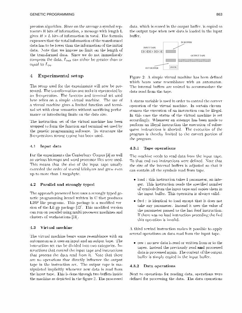
pression algorithm. Since on the average a symbol rep-

resents H bits of information, a message with length L

gives H � L bits of information in total. The formula

expresses that the total information of the transformed

data has to be lower than the information of the initial

data. Note that we impose no limit on the length of

the transformed data. Since we do not immediately

compress the data, Lout can either be greater than or

equal to Lin.

4 Experimental setup

The setup used for the experiments will now be pre-

sented. The transformation one seeks is represented by

an S-expression. The function and terminal set used

here relies on a simple virtual machine. The use of

a virtual machine gives a limited function and termi-

nal set with clear semantics without sacri�cing perfor-

mance or introducing limits on the data size.

The instruction set of the virtual machine has been

wrapped to form the function and terminal set used by

the genetic programming software. To structure the

S-expressions strong typing has been used.

4.1 Input data

For the experiments the Canterbury Corpus [3] as well

as various bitmaps and word processor �les were used.

This means that the size of the input tape usually

exceeded the order of several kilobytes and grew even

up to more than 1 megabyte.

4.2 Parallel and strongly typed

The approach presented here uses a strongly typed ge-

netic programming kernel written in C that produces

LISP-like programs. This package is a modi�ed ver-

sion of the Lil-gp package [12]. This modi�ed version

can run on parallel using multi processor machines and

clusters of workstations [11].

4.3 Virtual machine

The virtual machine bears some resemblance with an

automaton as it uses an input and an output tape. The

instruction set can be divided into two categories. In-

structions that control the input tape and instructions

that process the data read from it. Note that there

are no operations that directly in uence the output

tape in the instruction set. The output tape is ma-

nipulated implicitly whenever new data is read from

the input tape. This is done through two bu�ers inside

the machine as depicted in the �gure 2. The processed

data, which is stored in the output bu�er, is copied to

the output tape when new data is loaded in the input

bu�er.

��

��OUTPUT TAPE

INPUT TAPE

IN BUFFER

OUT BUFFER INSTR

Figure 2: A simple virtual machine has been de�ned

which bears some resemblance with an automaton.

The internal bu�ers are resized to accommodate the

data read from the tape.

A status variable is used in order to control the correct

operation of the virtual machine. In certain circum-

stances the execution of an instruction can be illegal.

In this case the status of the virtual machine is set

accordingly. Whenever an attempt has been made to

perform an illegal instruction the execution of subse-

quent instructions is aborted. The execution of the

program is thereby limited to the correct portion of

the program.

4.3.1 Tape operations

The machine needs to read data from the input tape.

To that end two instructions were de�ned. Note that

the size of the internal bu�ers is adjusted so that it

can contain all the symbols read from tape.

� load : this instruction takes 1 parameter, an inte-

ger. This instruction reads the speci�ed number

of symbols from the input tape and copies them in

the input bu�er. This operation is always valid.

� fwd : is identical to load except that it does not

take any parameter. Instead it uses the value of

the parameter passed to the last load instruction.

If there was no load instruction preceding the fwd

this operation is invalid.

A third rewind instruction makes it possible to apply

several operations on data read from the input tape.

� rew : no new data is read or written from or to the

tapes. Instead the previously read and processed

data is processed again. The content of the output

bu�er is simply copied in the input bu�er.

4.3.2 Data operations

Next to operations for reading data, operations were

de�ned for processing the data. The data operations


are performed on the data present in the input bu�er.

Data produced by data operation is stored in the out-

put bu�er.

Since we are working with lossless compression each

of the data operations needs to be reversible. Each of

these operations needs to be reversible in order to be

useful within the lossless compression context. Hence,

for each data operation there is a reverse operation

de�ned in the virtual machine. These operations are

however not made available in the instruction set of

the genetic programming software.

The choice of the data operations was guided by their

capability to reduce the entropy of the data. This is

typical done by exploiting patterns that exist in the

data. A stride parameter was introduced for some op-

erations. The stride speci�es the step size when going

over the data. For example all the symbols 3 positions

apart (in this case the stride would be 3). The stride

allows data operations to work on patterns that may

be spread within the data.

� dpcm : stands for di�erential pulse code modula-

tion. fx0; x1; x2; x3; . . . , xng ) fx0; x1�x0; x2�x1; x3 � x2; . . . , xn � xn�1g This operation has a

stride parameter.

� min : This operation uses the average of all

the symbols (binary representation) in the input

bu�er. A symbol is replaced by the di�erence be-

tween the average and the symbol. This operation

does expand the data by 1 symbol, the symbol

which represents the average4.

fx0; x1; x2; x3; . . . , xng ) fxavg ; x0 � xavg ; x1 �xavg ; x2 � xavg ; x3 � xavg ; . . . , xn � xavgg This

operation has a stride parameter.

� raw : no transformation is applied at all to the

data. fx0; x1; x2; x3; . . . , xng ) fx0; x1; x2; x3;. . . , xng This may seem like a quite useless in-

struction. But it allows for jumps in the data

processing since we maybe do not need to trans-

form the entire tape. An alternative would be the

de�nition of a jump tape instruction.

� pec : pseudo exponential code. This operation

produces an output with double size of the input.

The output data represents an input symbol as

a couple of numbers. The output is based on the

number of the input symbol. A couple is a pseudo

exponent and a pseudo remainder. The pseudo

exponent is the largest exponent used as a power

4min (stride=1) changes the series 2 5 3 2 5 6 7 to -2 1 -1 1 2 3 + 4 (the average)

of 2 which doesn't exceed the input number, e.g.

3 for 10. The remainder is the di�erence between

the power of two and the input number, in the

previous example this would be 2 (10 - 2 3). The

reason for calling this pseudo5 is that it has been

modi�ed for numbers bigger than 128.

� mtf : move to front. This operation is a stan-

dard encoding scheme which uses a map of all

the possible symbols. The symbols are replaced

by their position in the map. Each time a sym-

bol is replaced by its current position in the map

the latter is updated. The symbol is put in front

of the map thereby assigning it a small number.

This allows to encode the symbols that appeared

recently with small numbers.

� inv : inversion. fx0; x1; x2; x3; . . . , xng) fMAX(x) � x0;MAX(x) � x1;MAX(x) �x2;MAX(x) � x3; . . . , MAX(x) � xng Here

MAX(x) represents the maximum value that can

be represent by the data type used to represent

the symbols. This operation has a stride parame-

ter.

� sub : substitution. This operation substitutes the

symbol that appears most frequently in the in-

put bu�er with the most frequent symbol in the

output tape so far. This operation has a stride

parameter.

4.4 Types

Typing is used in the �rst place to structure the pro-

grams that can be evolved. Evaluating the functions

and terminals corresponds to the execution of an in-

struction by the virtual machine. For the experiments

four types were used for the functions and terminals

of the genetic programming software. The �rst two

types are integer types, int and num. The num type

represents small integers in the range [0,20]. In order

to integrate the instruction of the machine two types

were de�ned for the operations: tape and data.

The reason for the de�nition of two separate types for

the instruction is the need to combine these instruc-

tions to make correct programs. Indeed, the data op-

erations are invalid when no data has been read from

the tape. And for the same reason tape operations

make no sense if the data is not processed afterwards.

5pec The symbols 1 123 250 are replaced by(3,4) (6,59) (13,58). The last couple allows to repre-sent 250 with two smaller numbers ( 27 + 26 +58) whereas log 2 would give the couple (7,122).


4.5 Function and terminal set

Here we present the function and terminal set provided

to the genetic programming system. Apart from the

operations provided by the virtual machine a few other

functionalities have been introduced.

The programs one can evolve consist of series of tape

operations. In order to obtain those series a special

function called SEQ has been used. The SEQ func-

tion will evaluate its �rst then its second arguments.

Arguments which in turn can be other SEQ functions

or real operations on the data.

The ERC INT and ERC NUM are used to create

ephemeral random constants. These values are either

used for the stride parameter expected by some data

operations or for the number of symbols to read from

tape using load. Related to this is the terminal END.

This terminal returns the number of symbols remain-

ing on the input tape. The introduction of this termi-

nal made it possible to evolve programs that processed

the entire input tape.

Table 1: Overview of the return types of the terminal

and function set.

Name ret type type arg1 type arg2

LOAD tape int data

FWD tape data /

REW tape data /

SEQ tape tape tape

END int / /

DPCM data num /

INV data num /

MIN data num /

SUB data num /

MTF data / /

RAW data / /

PEC data / /

DIV int int num

ERC INT int / /

ERC NUM num / /

4.6 Parameter settings

The experiments presented here were done using 2

populations of 500 individuals. The selection prob-

abilities of the di�erent genetic operations were:

� standard uniform subtree crossover 75%

� standard uniform mutation 20%

� reproduction 5%

� no depth or node count limit

� The selection strategy for the 3 genetic operators

was tournament selection with a tournament size

of 4

The island model requires additional parameters:

� exchange rate of 3 individuals every 10 genera-

tions

� the exchanged individuals (the ones being ex-

ported) were selected using tournament selection

� The worst individuals in destination subpopula-

tion were replaced by the imported ones

5 Results

5.1 Tool-box and decoder

To validate the presented results a set of software tools

have been implemented. The functions and terminals

needed by the gp software are provided by an imple-

mentation of the virtual machine.

In order to reverse the transformation an encoding for-

mat has also been designed. When executing an in-

struction, the data produced by the virtual machine

actually comprises a header and the processed input

data. This header describes the instruction used to

produce the data, the length of the data as well as

possible parameters required by the instruction. In

the present implementation this header is 9 bytes in

size. It is important to point out that the program

that produced the transformed data is encoded in the

output data. The entropy used as an objective crite-

rion in the �tness function, is thus the entropy of the

data and the program that created it.

Of course a decoder is required to reconstruct the orig-

inal data. Using the headers present in the data the

di�erent transformations can be reversed one by one.

One can decode the preprocessed �les and compare

them with the original data with a program such as

di�. The size of the statically linked decoder is 23534

bytes on a Linux x86 platform. Both the data and the

decoder should be transmitted to obtain the original

data. The gain in compression should exceed the size

of the decoder.

5.2 Entropy reduction

Files from the Canterbury Corpus were used as input

data and a separate preprocessor evolved for each of

them. The reduction of the entropy obtained for some


of the �les is given in table 2. The standard image

compression image lena, for example, has been trans-

formed so that is retains only 68.3% of its original

entropy. And this without any loss of information.

Table 2: Comparison between the initial entropy and

the entropy after preprocessing

File original H new H % reduction

kennedy.xls 3.57 0.7 78.4

laptop.bmp 7.76 3.3 56.5

lena std.ppm 7.75 5.2 31.7

mosaic.pnm 7.78 4.1 46.6

peppers.ppm 7.66 5.3 30.1

This reduction in entropy without loss of information

is not impossible. The evolved preprocessor exploits

the redundancy that is present in the data. This can

not be modeled by the formula for the entropy given by

equation 2. One would have to use conditional proba-

bilities when computing the entropy to account for this

kind of redundancy. This higher order redundancy is

however very much there and is (partially) exposed by

transforming the data. Although reducing the entropy

of given data is not an easy task, it is of no immedi-

ate use as such. The idea behind reducing the entropy

is to improve the compression rate. To illustrate this

table 3 gives a comparison between the compression

ratio of the data with and without preprocessing. The

compression algorithm used here is bzip2. 6

Table 3: Di�erence in compression ratio after prepro-

cessing. Initially the lena could be compressed to 74%

of its initial size. After preprocessing the compression

ration is 68% of the size.

File ratio new ratio % reduction

kennedy.coded 0.12 0.02 80.8

laptop.coded 0.53 0.43 19.1

lena std.coded 0.74 0.68 7.9

mosaic.coded 0.72 0.52 28.3

peppers.coded 0.80 0.69 14.3

One can notice some di�erence between the gain in

entropy and the gain in compression size. The gain in

compressed size can be smaller than the reduction in

6Bzip2 is free implementation of the Burrows-Wheelertransform. Bzip2 was invoked with the maximum compres-sion parameter -9.

entropy because Burrows Wheeler transform [1] used

by bzip2 can to some extent model the redundancy be-

yond the single symbol probabilities. In other words,

bzip2 already breaks the theoretical limit computed

using the entropy formula in equation 2. That is why

the gain is somewhat lower in this case.

5.3 Filters

It was initially expected that, given the operations

which can process chunks of data, the evolved pro-

grams would process the entire input data in a piece-

wise manner. That is, the programs would consist of a

sequence of operations on contiguous parts of the data.

The function set provided to the genetic programming

framework certainly would allow for such programs to

be evolved.

This was however not the case, in the �rst experiments

only small fractions of the data were being processed.

In their experiments Nordin and Banzhaf [10] have

chosen to evolve separate programs for segments of

�xed size, chunking, to avoid a similar problem.

The reason behind this phenomenon is that the en-

tropy is a global measure over the entire output tape.

Initial programs may indeed reduce the entropy. But

the growth of these programs can adversely a�ect the

initial changes to the entropy. Thereby making the

results of the genetic operations like crossover less �t.

This has been observed even when the initial popula-

tion was seeded with full grown trees.

(SEQ (SEQ (SEQ (LOAD (DIV 67 2)(DPCM 1))

(SEQ (LOAD END (DPCM 1))

(REW (DPCM 3))))

(SEQ (REW (SUB 1))

(REW (DPCM 3))))

(SEQ (REW (SUB 1))

(REW (DPCM 3))))

However with the introduction of the special END

terminal in the set an interesting result showed up.

This dynamic terminal returns the number of symbols

left on the input tape. The evolved programs became

�lters. Most of the data goes through several trans-

formations. In the example above, the program can

be divided in 2 parts. First, 33 symbols are load into

the machine and DPCM coded using the (LOAD (DIV

67 2) (DPCM 1)) instruction. The second part of the

program processes far more symbols. The instruction

(LOAD END (DPCM 1)) instruction loads all the sym-

bols remaining on the input tape and DPCM codes

these. Using the (REW (DPCM 3)) instruction the

DPCM coded data is used again as input. This time

the data is DPCM coded again but only every 3-th


symbol is being processed. The data will undergo 4

more transformation after this step. The remain trans-

formation are in order: SUB, DPCM, SUB, DPCM.

0.46

0.48

0.5

0.52

0.54

0.56

0.58

0.6

0.62

0.64

0 20 40 60 80 100

Adj

uste

d fit

ness

Generation

Enhancement for different images

peppers.ppmmosaic.ppmlaptop.bmp

lena_std.ppm

Figure 3: Evolution of the adjusted �tness of the best

individual for the di�erent data �les, average of 8 runs.

6 Conclusion

This experiment presents a new approach for combin-

ing genetic programming and lossless data compres-

sion. The chosen approach develops preprocessing pro-

grams which are tailored to the data one wishes to

compress. The obtained results are encouraging both

in terms of gain in compression as for the computation

time required to evolve the programs. One should note

that, although the experiments were done using a par-

allel software package, the speed improvement results

from the �tness function as well as the fact that we

focus on preprocessors. Surprisingly the evolved pro-

grams were mostly �lters although the provided func-

tions and terminals allowed to evolve to more complex

preprocessors.

References

[1] M. Burrows and D.J. Wheeler. A block-sorting

lossless data compression algorithm. Digital Sys-

tem Research Center research report 124, 1994.

[2] Winzip Corporation. www.winzip.com.

[3] Canterbury Corpus.

http://corpus.canterbury.ac.nz/.

[4] Karel Driesen. Compressing sparse tables using a

genetic algorithm. In Proceedings of the GRON-

ICS'94 Student Conference, Groningen, February

1994.

[5] I. De Falco et al. A kolmogorov complexity-base

genetic programming tool for string compression.

In Proceedings Seventh International Conference

on Genetic Algorithms (ICGA97), 1997.

[6] H. Feiel and S. Ramakrishnan. A genetic ap-

proach to color image compression. In ACM 0-

89791-850-9, 1997.

[7] Alex Fukunaga and Andre Stechert. Evolving

nonlinear models for lossless image compression

with genetic programming. In Genetic Program-

ming 1998: Proceedings of the Third Annual Con-

ference, pages 92{102, 1998.

[8] The Gzip homepage. www.gzip.org.

[9] Sean Luke. Code growth is not caused by introns.

In Late Breaking Papers at the 2000 Genetic and

Evolutionary Conference, 2000.

[10] Peter Nordin and Wolfgang Banzhaf. Program-

matic compression of images and sound. In David

B. Fogel John R. Koza, Davis E. Goldberg and

Stanford University Rick L. Riolo ed., editors,

Proceedings of the First Annual Conference on

Genetic Programming, pages 354{350. CA, USA,

Mit Press.

[11] J. Parent. Parallel lil-gp techni-

cal report. Vrije Universiteit Brussel,

http://parallel.vub.ac.be./~johan/Projects/.

[12] B. Punch and D. Zonker. lil-gp genetic pro-

gramming version 1.1 beta. michigan state uni-

versity, http://garage.cps.msu.edu/software/lil-

gp/index.html.

[13] P. Vitanyi. An Introduction to Kolmogorov Com-

plexity and Its Applications. Addison-Wesley,

Reading, Mass, 1991.


On the Search Biases of Homologous Crossover in Linear GeneticProgramming and Variable-length Genetic Algorithms

Riccardo PoliDepartment of

Computer ScienceUniversity of Essex, UK

[email protected]

Christopher R. StephensInstituto de

Ciencias NuclearesUNAM, Mexico

[email protected]

Alden H. WrightComputer Science

DepartmentUniversity of Montana, USA

[email protected]

Jonathan E. RoweSchool of

Computer ScienceUniversity of Birmingham, UK

[email protected]

Abstract

With a schema-theoretic approach and experi-ments we study the search biases produced byGP/GA homologous crossovers when appliedto linear, variable-length representations. Byspecialising the schema theory for homologouscrossovers we show that these operators are unbi-ased with respect to string length. Then, we pro-vide a fixed point for the schema evolution equa-tions where the population presents a statisticallyindependent distribution of primitives. This is animportant step towards generalising Geiringer’stheorem and the notion of linkage equilibrium.

1 INTRODUCTION

Search algorithms typically include three main steps whichare iterated in succession: choosing one or multiple pointsof the search space the neighbourhood of which to explorefurther, applying expansion operators to obtain a new setof points, deciding what to do with the points previouslyvisited and with the newly generated ones. For example, inthe case of genetic algorithms and genetic programming,selection corresponds to the first task, crossover and muta-tion are the expansion operators, and the replacement strat-egy corresponds to the third task. Note that many moresteps may be included if one looks at search algorithms ata finer level of abstraction (Poli & Logan, 1996), but thisis not particularly important for the purposes of this dis-cussion. What is important is that different algorithms willuse different strategies to realise the different steps. Thisleads to the sampling of the search space according to dif-ferent schedules. With the exception of random search, thismeans that some areas of the search space will be exploredsooner, will be allocated more samples, or will be ignoredaltogether. This is what we mean by search bias.

Clearly the bias of an algorithm is the result of the interac-tion of the biases of all its components. In the case of fixed

length genetic algorithms, a lot of attention has been de-voted to the biases of all such components: selection, muta-tion and crossover, and replacement. Some of the resultingstudies apply also to the case of variable-length-structureevolution. For example, the focusing effects of selectionwill be exactly the same, since selection is representation-independent. However, very little is known about the biasesof the genetic operators used to evolve variable length rep-resentations, such as those used in linear GP (Nordin, 1994;O’Neill & Ryan, 2001) or in variable-length GAs.

Knowing the biases introduced by the operators is veryimportant, since it leads to a deeper understanding of thesearch algorithm under investigation. This, in turn, allowsan informed choice of operators, parameter settings andeven initialisation strategies for particular problems. Howcan one investigate these biases? One possibility is to usecarefully designed empirical studies. In the past these haveshed some light on the internal dynamics of GP (e.g. onbloat (McPhee & Miller, 1995; Soule et al., 1996; Lang-don et al., 1999)), but rarely has the evidence been generaland conclusive. This is because these studies can only con-sider a limited number of benchmark problems, and so itis impossible to know whether, and to which extent, theobserved behaviour is applicable to other problems. An al-ternative is to perform theoretical studies. Often these maylead to more general and precise conclusions, but they aredefinitely much harder and slower to carry out. Also, some-times the complexity of the mathematics involved in thesestudies forces the researcher to make simplifying hypothe-ses which may limit the explanatory power of the results.

A class of recent theoretical results which require veryfew, if any, simplifications goes under the name of exactschema theorems.1 These provide probabilistic models (theschema evolution equations) of the expected behaviour ofa GA or a GP system over one, or, under certain assump-tions, multiple generations (Poli, 2001b; Langdon & Poli,

1The word “exact” refers to the fact that, unlike earlier results,these theorems provide an exact value, rather than a lower bound,for the expected number of individuals in a schema in the nextgeneration.


2002). The main advantage of these exact models is thatthey provide a natural way of coarse graining the hugenumber of degrees of freedom present in a genetic algo-rithm (Stephens & Waelbroeck, 1997). Exact schema theo-rems have recently become available for fixed-length GAswith one-point crossover and mutation (Stephens & Wael-broeck, 1997; Stephens & Waelbroeck, 1999), and generalhomologous crossover and mutation (Vose & Wright, 2001;Stephens, 2001). Even more recent is the developmentof exact schema theorems for variable-length GAs, linearGP and tree-based GP. These cover a variety of crossoverand mutation operators including one-point crossover (Poli,2000; Poli, 2001b), subtree-swapping crossovers (Poli,2001a; Poli & McPhee, 2001b; McPhee & Poli, 2001),different types of subtree mutation and headless chickencrossover (Poli & McPhee, 2001a; McPhee et al., 2001),and homologous crossovers (Poli & McPhee, 2001c).

These exact models can be used to understand an evolution-ary system and study its behaviour in two different ways.This can be done either through simulation (i.e., by numeri-cally iterating the equations) or through mathematical anal-ysis. Although exact GP schema equations have becomeavailable only very recently, early studies indicate their use-fulness, for example, in providing a deeper understandingof emergent phenomena such as bloat (Poli & McPhee,2001b; McPhee & Poli, 2001). Also, in general, as indi-cated above the availability of exact models for differentoperators allows a formal study of the biases of those op-erators. Steps forward in this direction have recently beenmade in (Poli & McPhee, 2001b; McPhee & Poli, 2001;McPhee et al., 2001), where a class of Gamma program-length distributions has been shown to represent a naturalattractor for variable-length linear systems under GP sub-tree crossover and in (Poli et al., 2002) where we have ex-tended the study to other biases of subtree crossover.

In this paper we study the biases of the whole class of ho-mologous GP crossover operators for the case of linear GPand variable-length GAs. These are a set of operators, in-cluding GP one-point crossover (Poli & Langdon, 1997)and GP uniform crossover (Poli & Langdon, 1998a), wherethe offspring are created preserving the position of the ge-netic material taken from the parents. These operators areimportant because they are the natural generalisation of thecorresponding GA operators. So, the theory presented hereis a generalisation of corresponding GA theory.

The paper is organised as follows. We start by provid-ing some background information on the exact GP schematheory for homologous crossover and Geiringer’s theoremin Sections 2 and 3. Then, we simplify the theory forthe case of linear, but variable-length, structures in Sec-tion 4, and show that homologous crossover is totally unbi-ased with respect to string length (Section 5). In Section 6we provide a fixed point for the schema evolution equa-tions which is a first step towards generalising Geiringer’s

theorem (Geiringer, 1944) and the notion of linkage equi-librium, which, until now, were applicable only to fixed-length representations. The fixed point and some experi-mental evidence (reported in Section 7) indicate the pres-ence of a bias which pushes the population towards a statis-tically independent distributions of primitives, as discussedin Section 8, where we also draw some conclusions.

2 SCHEMA THEORY BACKGROUND

Schemata are sets of points in a search space sharing somesyntactic feature. For example, for GAs operating on bi-nary strings the syntactic representation of a schema is usu-ally a string of symbols from the alphabet f0,1,*g, wherethe character * is interpreted as a “don’t care” symbol. Typ-ically schema theorems are descriptions of how the numberof members of the population belonging to a schema varyover time. If �(H; t) denotes the probability that at time t anewly created individual samples (or matches) the schemaH , which we term the total transmission probability of H ,then an exact schema theorem for a generational system issimply

E[m(H; t+ 1)] =M�(H; t);

where M is the population size, m(H; t + 1) is the num-ber of individuals sampling H at generation t + 1 andE[�] is the expectation operator. Holland’s (Holland, 1975)and other (e.g. (Poli & Langdon, 1998b)) worst-case-scenario schema theories normally provide a lower boundfor �(H; t) or, equivalently, for E[m(H; t + 1)]. How-ever, recently exact schema theorems (Stephens & Wael-broeck, 1997; Stephens & Waelbroeck, 1999; Poli, 2000;Poli, 2001b; Poli, 2001a; Poli & McPhee, 2001b; McPhee& Poli, 2001; Poli & McPhee, 2001a; McPhee et al., 2001;Stephens, 2001; Poli & McPhee, 2001c) which provide theexact value for �(H; t) have become available for GAs andGP with a variety of operators. In the remainder of thissection we will introduce the various elements which arenecessary to understand the exact schema equations for GPhomologous crossover, since these will be the starting pointfor the new results in this paper.

Let us start from our definition of schema for GP. Syntac-tically a GP schema is a tree composed of functions fromthe set F [f=g and terminals from the set T [f=g, whereF and T are the function and terminal sets used in a GPrun. The primitive= is a “don’t care” symbol which standsfor a single terminal or function. A schema H representsthe set of all programs having the same shape as H and thesame non-= nodes as H . Particularly important for the GPschema theory are schemata containing “don’t care” sym-bols only, since they represent all the programs of a par-ticular shape. Let G1, G2, � � � be an enumeration of suchshape-representing schemata.

In GP homologous crossovers the offspring are createdby exchanging genetic material (nodes and subtrees) taken


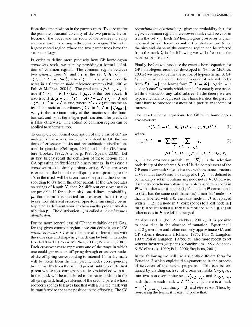
from the same position in the parents trees. To account forthe possible structural diversity of the two parents, the se-lection of the nodes and the roots of the subtrees to swapare constrained to belong to the common region. This is thelargest rooted region where the two parent trees have thesame topology.

In order to define more precisely how GP homologouscrossovers work, we start by providing a formal defini-tion of common region. The common region betweentwo generic trees h1 and h2 is the set C(h1; h2) =f(d; i)jC(d; i; h1; h2)g, where (d; i) is a pair of coordi-nates in a Cartesian node reference system (Poli, 2001a;Poli & McPhee, 2001c). The predicate C(d; i; h1; h2) istrue if (d; i) = (0; 0) (i.e., if (d; i) is the root node). Italso true if A (d� 1; i0; h1) = A (d� 1; i0; h2) 6= 0 andC (d� 1; i0; h1; h2) is true, where A(d; i; h) returns the ar-ity of the node at coordinates (d; i) in h, i0 = bi=amaxc,amax is the maximum arity of the functions in the func-tion set, and b�c is the integer-part function. The predicateis false otherwise. The notion of common region can beapplied to schemata, too.

To complete our formal description of the class of GP ho-mologous crossovers, we need to extend to GP the no-tions of crossover masks and recombination distributionsused in genetics (Geiringer, 1944) and in the GA litera-ture (Booker, 1992; Altenberg, 1995; Spears, 2000). Letus first briefly recall the definition of these notions for aGA operating on fixed-length binary strings. In this case acrossover mask is simply a binary string. When crossoveris executed, the bits of the offspring corresponding to the1’s in the mask will be taken from one parent, those corre-sponding to 0’s from the other parent. If the GA operateson strings of length N , then 2N different crossover masksare possible. If, for each mask i, one defines a probability,pi, that the mask is selected for crossover, then it is easyto see how different crossover operators can simply be in-terpreted as different ways of choosing the probability dis-tribution pi. The distribution pi is called a recombinationdistribution.

For the more general case of GP and variable-length GAs,for any given common region c we can define a set of GPcrossover masks, �c, which contains all different trees withthe same size and shape as c which can be built with nodeslabelled 0 and 1 (Poli & McPhee, 2001c; Poli et al., 2001).Each crossover mask represents one of the ways in whichone could generate an offspring through crossover: nodesof the offspring corresponding to internal 1’s in the maskwill be taken from the first parent, nodes correspondingto internal 0’s from the second parent, subtrees of the firstparent whose root corresponds to leaves labelled with a 1in the mask will be transferred to the same position in theoffspring, and, finally, subtrees of the second parent whoseroot corresponds to leaves labelled with a 0 in the mask willbe transferred to the same position in the offspring. The GP

recombination distribution pcl gives the probability that, fora given common region c, crossover mask l will be chosenfrom the set �c. Each GP homologous crossover is char-acterised by a different recombination distribution. Sincethe size and shape of the common region can be inferredfrom the mask l, in the following we will often omit thesuperscript c from p

cl .

Finally, before we introduce the exact schema equation forGP homologous crossover developed in (Poli & McPhee,2001c) we need to define the notion of hyperschema. A GPhyperschema is a rooted tree composed of internal nodesfrom F [ f=g and leaves from T [ f=;#g. Again, = isa “don’t care” symbols which stands for exactly one node,while # stands for any valid subtree. In the theory we usehyperschemata to represent the characteristics the parentsmust have to produce instances of a particular schema ofinterest.

The exact schema equations for GP with homologouscrossover are

�(H; t) = (1� pxo)p(H; t) + pxo�xo(H; t) (1)

where

�xo(H; t) =Xj

Xk

Xl2�C(Gj ;Gk)

pl (2)

p(�(H; l) \Gj ; t)p(�(H; �l) \Gk; t);

pxo is the crossover probability, p(H; t) is the selectionprobability of the schema H and �l is the complement of theGP crossover mask l (i.e. it is a tree with the same structureas l but with the 0’s and 1’s swapped). �(H; l) is defined tobe the empty set if l contains any node not in H . Otherwiseit is the hyperschema obtained by replacing certain nodes inH with either = or # nodes: (1) if a node in H correspondsto (i.e., has the same coordinates as) a non-leaf node in l

that is labelled with a 0, then that node in H is replacedwith a =, (2) if a node in H corresponds to a leaf node in lthat is labelled with a 0, then it is replaced with a #, (3) allother nodes in H are left unchanged.

As discussed in (Poli & McPhee, 2001c), it is possibleto show that, in the absence of mutation, Equations 1and 2 generalise and refine not only approximate GA andGP schema theorems (Holland, 1975; Poli & Langdon,1997; Poli & Langdon, 1998b) but also more recent exactschema theorems (Stephens & Waelbroeck, 1997; Stephens& Waelbroeck, 1999; Poli, 2000; Stephens, 2001).

In the following we will use a slightly different form forEquation 2 which exploits the symmetries in the processof selection of the parent programs. This can be ob-tained by dividing each set of crossover masks �C(Gj;Gk)into two non-overlapping sets �0

C(Gj;Gk)and ��0

C(Gj;Gk)

such that for each mask x 2 �0C(Gj;Gk)

, there is a mask

y 2 ��0C(Gj;Gk)

such that y = �x, and vice versa. Then, byreordering the terms, it is easy to prove that:


Theorem 1.

�xo(H; t) =Xj

Xk

Xl2�0

C(Gj ;Gk)

(pl + p�l) (3)

p(�(H; l) \Gj ; t)p(�(H; �l) \Gk; t)

3 GEIRINGER’S THEOREM

In this section we briefly introduce Geiringer’s theo-rem (Geiringer, 1944), an important result with implica-tions both for natural population genetics and evolutionaryalgorithms (Booker, 1992; Spears, 2000). Geiringer’s the-orem indicates that, in a population of fixed-length chro-mosomes repeatedly undergoing crossover (in the absenceof mutation and selective pressure), the probability of find-ing a generic string h1h2 � � �hN approaches a limit distri-bution which is only dependent on the distribution of thealleles h1, h2, etc. in the initial generation. More precisely,if �(h1h2 � � �hN ; t) is the proportion of individuals of typeh1h2 � � �hN at generation t and �(hi; t) is the proportionof individuals carrying allele hi then

limt!1

�(h1h2 � � �hN ; t) =NYi=1

�(hi; 0): (4)

This result is valid for all homologous crossover operatorswhich allow any two loci to be separated by recombina-tion. Strictly speaking the result is valid only for infinitepopulations.

If one interprets �(h1h2 � � �hN ; t) as a probability distri-bution of the possible strings in the population, we caninterpret Equation 4 as saying that such a distribution isconverging towards independence. When, at a particulargeneration t, the frequency of any string in a population�(h1h2 � � �hN ; t) equals

QN

i=1�(hi; t), the population issaid to be in linkage equilibrium or Robbins’ proportions.

It is trivial to generalise Geiringer’s theorem to obtainthe expected fixed-point proportion of a generic linearfixed-length GA schema H for a population undergoingcrossover only:

limt!1

�(H; t) =Y

i2�(H)

�(�i�1hi�N�i

; 0); (5)

where �(H) is the set of indices of the defining symbolsin H , hi is one such defining symbols and we used thepower notation xy to mean x repeated y times. (Note that�(�i�1hi�

N�i; t) coincides with �(hi; t).)

4 EXACT SCHEMA THEORY FORLINEAR STRUCTURES

As indicated in Section 1 in this paper we will consider thebiases of the homologous crossovers in the case of variable-

size linear representations. We start by specialising Equa-tion 3 to this case.

When only unary functions are used in tree-basedGP, schemata (and programs) can only take the form(h1(h2(h3::::(hN�1hN )::::))) whereN > 0, hi 2 F[f=gfor 1 � i < N , and hN 2 T [ f=g. Therefore, they canbe written unambiguously as strings of symbols of the formh1h2h3::::hN�1hN . It should be noted that these strings ofsymbols do not have to be necessarily interpreted as rep-resenting programs. If one uses a special terminal set Tincluding only one terminal, say EOR (for End Of Repre-sentation), which will be ignored when the representationis interpreted, then strings of the form h1h2h3::::hN�1hN

can be interpreted as chromosomes of length N � 1 (sincehN can only be EOR). So, if F = f0; 1g, where 0 and 1 are“unary functions”,2 our GP system will explore the spaceof variable length binary strings. If instead F includesthe “unary functions” fADD R0 R1;MUL R0 R1; : : :g,then our tree-based GP system explores the same searchspace as a machine-code GP system with the same primi-tive set (Nordin & Banzhaf, 1995). So, in general our spe-cialisation of Equation 3 will be valid for variable-lengthGAs and linear GP.

In the specialisation to the linear case we replace the “don’tcare” symbol “=” with the more standard symbol “*”. Also,as we did previously, we represent repeated symbols ina string using the power notation. Since in this case alltrees are linear, the space of program shapes can be enu-merated by fGng where Gn is �n for n > 0. Given this,the common region between shapes Gj and Gk is simplythe shorter of the two schemata, i.e. C(Gj ; Gk) = Gj#k =�j#k where the operator # returns the minimum of its twoarguments. Therefore, the set of crossover masks in thecommon region, �C(Gj ;Gk) = �

�j#k , can be identified withthe set f0; 1gj#k. Below we will use N(l) to denote thelength of mask l, and the notation li to indicate the i-thelement of bitmask l. We will also use the operators

a � b =

�a if b = 1* otherwise,

a1a2 � � � Æ b =

�a1a2 � � � if b = 1# otherwise,

where a and b are bits, a1a2 � � � is a bit string and # standsfor any sequence of at least one primitive. With this no-tation, it is easy to show that, in a linear representation, ifN(l) > N then�(H; l) is the empty set and�(H; l)\Gj =; \ �j = ;. If N(l) � N , �(H; l) is

(h1 � l1) � � � (hN(l)�1 � lN(l)�1)(hN(l) � � �hN Æ lN(l))

and

2We are not interested in the output of these functions, butsimply in their topological organisation within the individual.


�(H; l) \Gj = �(H; l) \ �j = (6)8>>><>>>:

(h1 � l1) � � � (hN(l)�1 � lN(l)�1)�j�N(l)+1

if j � N(l) and lN(l) = 0;

(h1 � l1) � � � (hN(l)�1 � lN(l)�1)hN(l) � � �hNif j = N and lN(l) = 1,

; otherwise.

Thus, p(�(H; l) \ Gj ; t) = 0 for all j 6= N for all themasks l for which lN(l) = 1. So, if we choose�0

C(Gj ;Gk)=

f0; 1gj#k�1�f1g, in Equation 3 only the terms for j = N

can be non-zero. Using this simplification and the previousresults, one can transform Equation 3 into:

Theorem 2. If �0�N#k = f0; 1gj#k�1 � f1g, then

�xo(h1:::hN ; t) =Xk>0

Xl2�0

�N#k

(pl + p�l) (7)

p((h1 � l1) � � � (hN#k�1 � lN#k�1)hN#k � � �hN ; t)

p((h1 � �l1) � � � (hN#k�1 � �lN#k�1)�k�N#k+1

; t):

5 LENGTH EVOLUTION

Equation 7 can be used to study, among other things, theevolution of size in linear GP/GA systems. This is becauseit can be specialised to schemata of the form �N obtaining:

�xo(�N; t) =

Xk>0

Xl2�0

�N#k

(pl + p�l) p(�N; t)p(�k; t)

= p(�N ; t)Xk>0

p(�k; t)X

l2�0

�N#k

(pl + p�l) :

ButP

l2�0

�N#k(pl + p�l) = 1 and

Pk>0 p(�

k; t) = 1, so:

Theorem 3.�xo(�

N; t) = p(�N ; t): (8)

This result indicates that in linear representations lengthevolves under homologous crossovers as if selection onlywas acting. So, homologous crossovers are totally unbiasedwith respect to program length. The lack of length bias ofhomologous crossovers is made particularly clear if one as-sumes a flat fitness landscape in which p(H; t) = �(H; t)for allH . In these conditions all the dynamics in the systemmust be caused by crossover or by sampling effects. In theinfinite population limit, the total transmission probability�(H; t) can also be interpreted as the proportion of individ-uals in the population in H at generation t+1,�(H; t+1).So, for an infinite population and a flat landscape Equa-tion 8 becomes �(�N ; t+ 1) = �(�N ; t), whereby

Corollary 4. For a flat landscape, an infinite populationand any t > 0

�(�N ; t) = �(�N ; 0):

This equation is important because it shows that when a ho-mologous crossover alone is acting, any initial distributionof lengths is a fixed point length distribution for the system.

6 EXTENSION OF GEIRINGER’STHEOREM

A full extension of Geiringer’s theorem to linear, variable-length structures and homologous GP crossover would re-quire two steps: (a) proving that, in the absence of mutationand of selective pressure and for an infinite population, adistribution �(h1h2 � � �hN ; t), where the alleles/primitivescan be considered independent stochastic variables, is afixed point, and (b) showing that the system indeed movestowards that fixed point. In this paper we prove (a) mathe-matically and provide experimental evidence for (b).

Theorem 5. A fixed point distribution for the proportion ofa linear, variable-length schema h1h2 � � �hN under homol-ogous crossover for an infinite population on a flat fitnesslandscape in the absence of mutation is

�(h1h2 � � �hN ; t) = �(�N�1hN ; 0)

N�1Yi=1

�(�i�1hi#; 0)

�(�i#; 0);

(9)where

�(�i�1hi#; 0) =Xn>0

�(�i�1hi�n; 0)

and�(�i#; 0) =

Xn>0

�(�i+n; 0):

Proof. Since the fitness landscape is flat, p(H; t) =�(H; t) for any schema. Also, because the population isinfinite, �(H; t) = �(H; t+1). So, combining Equations 1and 7 yields

�(h1:::hN ; t+ 1) (10)

= (1� pxo)�(h1:::hN ; t) + pxo

Xk>0

Xl2�0

�N#k

(pl + p�l)

� �((h1 � l1) � � � (hN#k�1 � lN#k�1)hN#k � � �hN ; t)

� �((h1 � �l1) � � � (hN#k�1 � �lN#k�1)�k�N#k+1

; t):

We prove that Equation 9 represents a fixed point for Equa-tion 10 by substituting the former in the latter and reorder-ing the terms, obtaining

�(h1:::hN ; t+ 1)

= (1� pxo)�(�N�1

hN ; 0)

N�1Yi=1

�(�i�1hi#; 0)

�(�i#; 0)

+ pxo�(�N�1

hN ; 0)Xk>0

�(�k; 0)


�X

l2�0

�N#k

(pl + p�l)

�

N#k�1Yi=1

��(�i�1(hi � li)#; 0)�(�

i�1(hi � �li)#; 0)

(�(�i#; 0))2

�

�N�1Yi=N#k

�(�i�1hi#; 0)

�(�i#; 0):

Whatever the value of bit li in the mask, either hi � li = hi

and hi � �li = �, or hi � li = � and hi � �li = hi. Ineither case �(�i�1(hi � li)#; 0)�(�

i�1(hi � �li)#; 0) =�(�i�1hi#; 0)�(�

i#; 0). So, after reordering the terms,we obtain:

�(h1:::hN ; t+ 1)

= (1� pxo)�(�N�1

hN ; 0)

N�1Yi=1

�(�i�1hi#; 0)

�(�i#; 0)

+ pxo�(�N�1

hN ; 0)

N�1Yi=1

�(�i�1hi#; 0)

�(�i#; 0)

�Xk>0

�(�k; 0)X

l2�0

�N#k

(pl + p�l)

= �(�N�1hN ; 0)

N�1Yi=1

�(�i�1hi#; 0)

�(�i#; 0)2

It is important to note that, although Equation 9 provides afamily of fixed points, this does not prove rigorously thatany population will always converge to one of them. Prov-ing this is complex and requires much more space than isavailable for this conference. We will provide the proofin a future more extended publication. Instead, in the fol-lowing section we will describe experimental results whichstrongly suggest that indeed populations move toward anindependent allele/primitive distribution.

7 EXPERIMENTAL RESULTS

In order to check the theoretical results in this paper weset up a population of variable length strings consisting of1,000,000 individuals. All individuals had the same termi-nal allele, 0, while two types of non-terminal alleles wereused: alleles of type 0 and alleles of type 1. The majorityof alleles were of type 0 and represented a “background”against which alleles of type 1 (the “contrast medium” weused to study the dynamics of non-terminal alleles) couldbe more easily traced. Initially, alleles of type 1 occupiedall the non-terminal loci of strings of a given length only(which was varied between experiments). The terminal lo-cus of those strings was occupied by an allele of type 0.All other terminal and non-terminal alleles in the popula-tion were of type 0.

In our experiments we used two different initial lengthdistributions: a Gamma distribution with mean 10.5, anda uniform distribution with lengths between 1 and 20.Each population was run for 100 generations. The systemwas a generational GP/GA system with either one-pointcrossover or uniform crossover (applied with 100% proba-bility) and a flat fitness landscape. One-point crossover is ahomologous crossover operator which, for variable lengthstrings, is characterised by the recombination distribution

p�n

l =n1=n if l 2 f0n; 10n�1; 110n�2; : : : ; 1n�10g,0 otherwise.

Uniform crossover has the recombination distributionp�n

l = 2�n.

Multiple independent runs were not required since the pop-ulation size was sufficiently large to remove any signifi-cant statistical variability and therefore to approximate theinfinite-population behaviour (for each program length wehad tens of thousands of individuals on average).

We start by checking what happens to the length distri-bution over time. Figure 1 shows that the distribution ofprogram length is at a fixed point when the population isinitialised using either a uniform length distribution or adiscrete Gamma distribution. This corroborates our findingthat any length distribution is a fixed point (Corollary 4).Note that the small variations in the plots are due to geneticdrift (i.e. a finite population effect).

Let us now consider the allele dynamics. Figure 2 showshow the distribution of alleles of type 1 varies over a num-ber of generations in a population initialised with the uni-form length distribution. In Figure 2(a) only strings oflength 2 included alleles of type 1 (in locus 1). However,under one-point crossover within a few generations (seeFigures 2(b) and (c)) the relative proportion of strings witha 1 in locus 1 reached the equilibrium value predicted byapplying Equation 9 to the schema 1�N�1:

limt!1

�(1�N�1; t)

�(�N ; 0)=

�(1#; 0)

�(�#; 0)

N�1Yi=2

�(�i�1 �#; 0)

�(�i#; 0)

�1201920

�N�1Yi=2

1 =1

19� 0:0526:

The same asymptotic value is approached when onlystrings of length 10 included alleles of type 1 at genera-tion 0, as shown in Figures 2(d)–(g). Qualitatively the be-haviour of other loci is the same, but the asymptotic valuesreached are slightly different, which is predicted by Theo-rem 5.

Figure 2 reveals that the speed with which alleles in dif-ferent loci approach their asymptotic value varies. Whilealleles in locus 1 move quickly towards their fixed point,the convergence speed decreases as the locus position in-


15

1015

20Locus 1

5

10

15

20

Program Length

0

0.2

0.4

0.6

0.8

1

Proportion(gen=0)

15

1015

20Locus 1

5

10

15

20

Program Length

00.010.020.030.040.050.060.070.080.09

Proportion One-point(gen=5)

15

1015

20Locus 1

5

10

15

20

Program Length

00.010.020.030.040.050.06


(a) (b) (c)

15

1015

20Locus 1

5

10

15

20

Program Length

0

0.2

0.4

0.6

0.8

1

Proportion(gen=0)

15

1015

20Locus 1

5

10

15

20

Program Length

00.10.20.30.40.50.60.70.8


15

1015

20Locus 1

5

10

15

20

Program Length

00.05

0.10.15

0.20.25

0.30.35

0.4


(d) (e) (f)

15

1015

20Locus 1

5

10

15

20

Program Length

00.010.020.030.040.050.060.070.080.09

0.1


15

1015

20Locus 1

5

10

15

20

Program Length

00.050.1

0.150.2

0.250.3

Proportion Uniform(gen=5)

15

1015

20Locus 1

5

10

15

20

Program Length

00.010.020.030.040.050.060.070.080.090.1

Proportion Uniform(gen=20)

(g) (h) (i)Figure 2: Plots of the relative proportion of non-terminal alleles of type 1 vs. locus position and program length for differentgenerations under different crossover operators. The population was initialised with a uniform length distribution, whereonly programs of length ` contained non-terminal alleles of type 1. The value of ` was 2 in (a)–(c) and 10 in (d)–(i).One-point crossover was used in (b), (c), (e), (f) and (g), uniform crossover in (h) and (i).

creases. This is due to the fact that alleles occupying non-terminal loci that are present in a large number of individu-als will be swapped more frequently than alleles occupyingloci present in a small number of individuals.

The behaviour of uniform crossover is almost identical.Analysis of our results revealed that the only difference isthe speed with which alleles in different loci approach theirasymptotic value. Uniform crossover mixes alleles morequickly as can easily be seen, for example, by comparingFigures 2(e) and (f) with Figures 2(h) and (i), respectively.

To further verify that under homologous crossover the pop-ulation tends towards an independent allele distribution, weperformed an experiment with exactly the same set up as inFigures 2(h) and (i) but this time we kept track of the co-occurrence of pairs of non-terminal alleles within the classof programs of length 10. So, for each generation we ob-tained a set of four 9�9 co-occurrence frequency matrices,

one for each possible choice of a pair of the non-terminalalleles 0 and 1. An element at position (r; c) of the co-occurrence matrix for non-terminal alleles a and b, repre-sented the average number of times allele a was present inlocus r while at the same time allele b was present in lo-cus c in strings of length 10. Once normalised by the totalnumber of strings of length 10, the diagonal elements of the0/0 and 1/1 matrices represent the proportions of alleles oftype 0 and 1, respectively, present at each locus.

For all allele pairs the co-occurrence matrices tended tothose predicted by the theory. For example, for the allelepair 0/0 the theoretical values for the off-diagonal elementscan be calculated using the following equation (obtainedfrom Equation 9)

limt!1

�(�a0 �b 0�10�a�b�2; t)

�(�10; 0)


0

10000

20000

30000

40000

50000

60000

70000

80000

2 4 6 8 10 12 14 16 18 20

Num

ber

of P

rogr

ams

Length

gen=0gen=5

gen=10gen=20gen=50

gen=100

(a)

0

10000

20000

30000

40000

50000

60000

70000

80000

5 10 15 20 25 30 35 40

Num

ber

of P

rogr

ams

Length

gen=0gen=5

gen=10gen=20gen=50

gen=100

(b)Figure 1: Plots of the number of programs vs. programlength for different generations for populations initialisedwith a uniform (a) and a Gamma (b) length distribution.

=�(�a0#; 0)

�(�a+1#; 0)�

�(�a+b+10#; 0)

�(�a+b+2#; 0)

�18�a20

19�a20

�17�a�b

2018�a�b

20

=18� a

19� a�

17� a� b

18� a� b:

These values are extremely close to the frequency of 0/0co-occurrence measured at generation 100 in our runs, theroot mean square error between the above-diagonal ele-ments being 0.004 (note that the co-occurrence matrix issymmetric). This is a tiny error considering that all fre-quencies were bigger than 0.8.

8 DISCUSSION AND CONCLUSIONS

Characterisations of the genetic biases of the operators(such as the ones offered in this paper and in (Poli et al.,2002)) are important because they allow the users ofGP/GA systems to evaluate whether their operators providethe desired search behaviour for the system. If this is notthe case, then the knowledge of the search biases of otheroperators allows for an informed choice for an alternative.

Here we have focused our attention on the biases of ho-mologous crossovers with respect to length and allele dis-tribution in a population of variable length linear structuresand presented theoretical results describing the asymptoticbehaviour for a GP/GA system evolving in a flat fitness

landscape. In addition, we have provided experimental evi-dence that firmly corroborates the theory, showing a perfectmatch (within experimental errors) between the predictionsof the theory based on generation 0 data and the observedlength and allele frequencies at later generations.

The behaviour we have observed and characterised is sim-ple: a) homologous crossovers are totally unbiased withrespect to program length, and b) crossover shuffles the al-leles present in different individuals and pushes the stringdistribution towards locus-wise independence.

A mixing behaviour is present in most crossover operatorsdescribed in the literature on fixed length GAs. It is wellknown that this destroys “linkage”, i.e. correlations, be-tween different allele positions in the population. In thefixed length case the asymptotic convergence towards in-dependence described by Geiringer’s theorem is the resultof the decay of correlations due to the mixing effect ofcrossover. Because the representation and operators con-sidered in this paper are generalisations of the correspond-ing fixed-length ones, it is not so surprising to see that lin-ear GP is also moving towards an independent fixed-pointstring distribution. In other words, allele mixing is the rea-son why the right hand side of Equation 9 is a product,like the right hand side of Equation 4. We have no reasonto believe that the situation would be significantly differ-ent in tree-based GP. Because our extension of Geiringer’stheorem is the result of specialising and studying the GPschema theorem’s equations, it is not unlikely that in thefuture we will be able to provide a Geiringer-like theoremfor tree-based GP.

Our theoretical results were obtained for the extreme caseof infinite populations and flat fitness landscapes. So, whyshould these be of any relevance to finite GP/GA popula-tions and realistic landscapes? Firstly, because the biasesof homologous crossovers in the absence of selection indi-cate the precise way in which this type of operators wouldnaturally tend to explore the search space. When selectionis added, the search bias will be modified by the focusingbias of selection, but, except in cases of very strong selec-tion, many of the features of the search bias shown on a flatlandscape will be retained. Secondly, because as shown inour experiments, the results obtained with real (but large)populations match very closely the infinite population the-ory. For smaller populations, the theory can still be used togive short term indications of the behaviour of the system.

Acknowledgements

CRS would like to thank the University of Birminghamfor a visiting Professorship and DGAPA-PAPIIT grantIN100201. RP and CRS would like to thank the Royal So-ciety and the University of Essex for their support. AldenWright did this work while visiting the University of Birm-ingham, supported by EPSRC grant GR/R47394.


References

Altenberg, L. (1995) The Schema Theorem and Price’s Theorem.In Foundations of Genetic Algorithms 3, (Whitley, L. D. &Vose, M. D., eds), pp. 23–49 Morgan Kaufmann, Estes Park,Colorado, USA.

Booker, L. B. (1992) Recombination distributions for genetic al-gorithms. In FOGA-92, Foundations of Genetic Algorithms,Vail, Colorado.

Geiringer, H. (1944) On the probability theory of linkage inMendelian heredity. Annals of Mathematical Statistics, 15(1), 25–57.

Holland, J. (1975) Adaptation in Natural and Artificial Systems.University of Michigan Press, Ann Arbor, USA.

Langdon, W. B. & Poli, R. (2002) Foundations of Genetic Pro-gramming. Springer.

Langdon, W. B., Soule, T., Poli, R. & Foster, J. A. (1999) The evo-lution of size and shape. In Advances in Genetic Programming3, (Spector, L., Langdon, W. B., O’Reilly, U.-M. & Angeline,P. J., eds),. MIT Press Cambridge, MA, USA pp. 163–190.

McPhee, N. F. & Miller, J. D. (1995) Accurate replication in ge-netic programming. In Genetic Algorithms: Proceedings of theSixth International Conference (ICGA95), (Eshelman, L., ed.),pp. 303–309 Morgan Kaufmann, Pittsburgh, PA, USA.

McPhee, N. F. & Poli, R. (2001) A schema theory analysis ofthe evolution of size in genetic programming with linear repre-sentations. In Genetic Programming, Proceedings of EuroGP2001 LNCS Springer-Verlag, Milan.

McPhee, N. F., Poli, R. & Rowe, J. E. (2001) A schematheory analysis of mutation size biases in genetic program-ming with linear representations. In Proceedings of the 2001Congress on Evolutionary Computation CEC2001 pp. 1078–1085 IEEE Press, COEX, World Trade Center, 159 Samseong-dong, Gangnam-gu, Seoul, Korea.

Nordin, P. (1994) A compiling genetic programming system thatdirectly manipulates the machine code. In Advances in GeneticProgramming, (Kinnear, Jr., K. E., ed.),. MIT Press pp. 311–331.

Nordin, P. & Banzhaf, W. (1995) Complexity compression andevolution. In Genetic Algorithms: Proceedings of the SixthInternational Conference (ICGA95), (Eshelman, L., ed.), pp.310–317 Morgan Kaufmann, Pittsburgh, PA, USA.

O’Neill, M. & Ryan, C. (2001) Grammatical evolution. IEEETransaction on Evolutionary Compuation, 5 (4).

Poli, R. (2000) Exact schema theorem and effective fitness for GPwith one-point crossover. In Proceedings of the Genetic andEvolutionary Computation Conference, (Whitley, D., Gold-berg, D., Cantu-Paz, E., Spector, L., Parmee, I. & Beyer, H.-G.,eds), pp. 469–476 Morgan Kaufmann, Las Vegas.

Poli, R. (2001a) General schema theory for genetic programmingwith subtree-swapping crossover. In Genetic Programming,Proceedings of EuroGP 2001 LNCS Springer-Verlag, Milan.

Poli, R. (2001b) Exact schema theory for genetic program-ming and variable-length genetic algorithms with one-pointcrossover. Genetic Programming and Evolvable Machines, 2(2), 123–163.

Poli, R. & Langdon, W. B. (1997) A new schema theory for ge-netic programming with one-point crossover and point muta-tion. In Genetic Programming 1997: Proceedings of the Sec-ond Annual Conference, (Koza, J. R., Deb, K., Dorigo, M.,Fogel, D. B., Garzon, M., Iba, H. & Riolo, R. L., eds), pp.278–285 Morgan Kaufmann, Stanford University, CA, USA.

Poli, R. & Langdon, W. B. (1998a) On the search properties ofdifferent crossover operators in genetic programming. In Ge-netic Programming 1998: Proceedings of the Third AnnualConference, (Koza, J. R., Banzhaf, W., Chellapilla, K., Deb,K., Dorigo, M., Fogel, D. B., Garzon, M. H., Goldberg, D. E.,Iba, H. & Riolo, R., eds), pp. 293–301 Morgan Kaufmann,University of Wisconsin, Madison, Wisconsin, USA.

Poli, R. & Langdon, W. B. (1998b) Schema theory for geneticprogramming with one-point crossover and point mutation.Evolutionary Computation, 6 (3), 231–252.

Poli, R. & Logan, B. (1996) The evolutionary computation cook-book: recipes for designing new algorithms. In Proceedingsof the Second Online Workshop on Evolutionary Computation,Nagoya, Japan.

Poli, R. & McPhee, N. F. (2001a) Exact GP schema theory forheadless chicken crossover and subtree mutation. In Proceed-ings of the 2001 Congress on Evolutionary Computation CEC2001, Seoul, Korea.

Poli, R. & McPhee, N. F. (2001b) Exact schema theorems forGP with one-point and standard crossover operating on linearstructures and their application to the study of the evolution ofsize. In Genetic Programming, Proceedings of EuroGP 2001LNCS Springer-Verlag, Milan.

Poli, R. & McPhee, N. F. (2001c) Exact schema theory for GP andvariable-length GAs with homologous crossover. In Proceed-ings of the Genetic and Evolutionary Computation Conference(GECCO-2001) Morgan Kaufmann, San Francisco, California,USA.

Poli, R., Rowe, J. E. & McPhee, N. F. (2001) Markov chainmodels for GP and variable-length GAs with homologouscrossover. In Proceedings of the Genetic and EvolutionaryComputation Conference (GECCO-2001) Morgan Kaufmann,San Francisco, California, USA.

Poli, R., Rowe, J. E., Stephens, C. R. & Wright, A. H. (2002)Allele diffusion in linear genetic programming and variable-length genetic algorithms with subtree crossover. In Proceed-ings of EuroGP 2002.

Soule, T., Foster, J. A. & Dickinson, J. (1996) Code growth in ge-netic programming. In Genetic Programming 1996: Proceed-ings of the First Annual Conference, (Koza, J. R., Goldberg,D. E., Fogel, D. B. & Riolo, R. L., eds), pp. 215–223 MITPress, Stanford University, CA, USA.

Spears, W. M. (2000) Limiting distributions for mutation and re-combination. In Proceedings of the Foundations of Genetic Al-gorithms Workshop (FOGA 6), (Spears, W. M. & Martin, W.,eds), Charlottesville, VA, USA.

Stephens, C. R. (2001) Some exact results from a coarse grainedformulation of genetic dynamics. In Proceedings of the Geneticand Evolutionary Computation Conference (GECCO-2001),(Spector, L., Goodman, E. D., Wu, A., Langdon, W. B., Voigt,H.-M., Gen, M., Sen, S., Dorigo, M., Pezeshk, S., Garzon,M. H. & Burke, E., eds), pp. 631–638 Morgan Kaufmann, SanFrancisco, California, USA.

Stephens, C. R. & Waelbroeck, H. (1997) Effective degrees offreedom in genetic algorithms and the block hypothesis. InProceedings of the Seventh International Conference on Ge-netic Algorithms (ICGA97), (Back, T., ed.), pp. 34–40 MorganKaufmann, East Lansing.

Stephens, C. R. & Waelbroeck, H. (1999) Schemata evolution andbuilding blocks. Evolutionary Computation, 7 (2), 109–124.

Vose, M. D. & Wright, A. H. (2001) Form invariance and implicitparallelism. Evolutionary Computation, 9 (3), 355–370.


Iterative Refinement of Computational Circuits using Genetic Programming

Matthew J. Streeter

Genetic Programming, Inc. Mountain View, California

[email protected]

Martin A. Keane Econometrics, Inc. Chicago, Illinois

[email protected]

John R. Koza Stanford University Stanford, California

[email protected]

Abstract Previous work has shown that genetic programming is capable of creating analog electrical circuits whose output equals common mathematical functions, merely by specifying the desired mathematical function that is to be produced. This paper extends this work by generating computational circuits whose output is an approximation to the error function associated with an existing computational circuit (created by means of genetic programming or some other method). The output of the evolved circuit can then be added to the output of the existing circuit to produce a circuit that computes the desired function with greater accuracy. This process can be performed iteratively. We present a set of results showing the effectiveness of this approach over multiple iterations for generating squaring, square root, and cubing computational circuits. We also perform iterative refinement on a recently patented cubic signal generator circuit, obtaining a refined circuit that is 7.2 times more accurate than the original patented circuit. The iterative refinement process described herein can be viewed as a method for using previous knowledge (i.e. the existing circuit) to obtain an improved result.

1 INTRODUCTION An analog electrical circuit whose output is a well-known mathematical function (e.g., square, square root) is called a computational circuit.

Analog computational circuits are especially useful when the mathematical function must be performed more rapidly than is possible with digital circuitry (e.g., for real-time signal processing at extremely high frequencies). Analog computational circuits are also useful when the need for a single mathematical function in an analog circuit does not warrant converting an analog

signal into a digital signal (using an analog-to-digital converter), performing the mathematical function in the digital domain (requiring a general purpose digital processor consisting of millions of transistors), and then converting the result to the analog domain (using a digital-to-analog converter).

The design of computational circuits is exceedingly difficult even for seemingly mundane mathematical functions. Success usually relies on the clever exploitation of some aspect of the underlying device physics of the components (e.g., transistors) that is uniquely suited to the particular desired mathematical function. Because of this, the implementation of each different mathematical function typically requires an entirely different design approach (Gilbert 1968, Sheingold 1976, Babanezhad and Temes 1986).

The topology of a circuit involves specification of the total number of components in the circuit, the identity of each component (e.g., resistor, transistor), and the connections between each lead of each component. Sizing involves the specification of the values (typically numerical) of each component possessing a component value (e.g., resistors, capacitors). Genetic programming (Koza 1992; Koza and Rice 1992; 1994a, 1994b) is a technique for automatically creating computer programs to solve, or approximately solve, problems. Genetic programming is an extension of the genetic algorithm (Holland 1975). Genetic programming is capable of synthesizing the design of both the topology and component values (sizing) for a wide variety of analog electrical circuits from a high-level statement of the circuit’s desired behavior and characteristics (Koza, Bennett, Andre, and Keane 1999; Koza, Bennett, Andre, Keane, and Brave 1999; Mydlowec and Koza 2000).

This paper extends previous work on synthesis of computational circuits using genetic programming by applying genetic programming in an iterative manner to obtain successively more accurate computational circuits. Specifically, we employ a multiple-run process in which each run involves generating a computational circuit that


produces as output an approximation to the error function (i.e. the difference between the target function and the circuit’s actual output) of the best-of-run circuit from the previous run.

Section 2 of this paper presents a proof-of-principle experiment involving iterative refinement of rational polynomial approximations to the sine function. Section 3 describes automatic synthesis of electrical circuits by means of developmental genetic programming. Section 4 itemizes the preparatory steps required to apply genetic programming to the problem of synthesizing computational circuits. Section 5 describes our experiments involving iterative refinement of squaring, square root, and cubing computational circuits. Section 6 describes an experiment involving iterative refinement of a post-2000 patented cubic signal generator circuit. Section 7 is the conclusion.

2 ITERATIVE REFINEMENT OF NUMERICAL APPROXIMATIONS TO FUNCTIONS

Iterative refinement as described in this paper can be applied to other problem areas involving the synthesis of structures or entities that generate a specified target curve as output. In particular, it can be applied to the problem of generating numerical approximations to mathematical functions. As a proof-of-principle experiment that could be conducted using relatively modest computational resources, we evolved successively more accurate rational polynomial approximations to the function sin(x) over the interval [0,π/2]. The function set for this problem consisted of the four arithmetic operators {+,*,-,%}. The terminal set consisted of the variable X and the random numeric terminal R. Fitness was defined as the sum of absolute error over 100 uniformly spaced points. We used a population size, M, of 100,000 and tournament selection with a tournament size of 10. The remaining control parameters are the same as those described in section 4.6 of this paper. Each run was conducted on a single Pentium workstation. A first run (iteration 0) was conducted using the target function sin(x). The best-of-run individual from this first run produces an output a0(x), with an associated error function defined as sin(x)-a0(x). We then perform a second run (iteration 1) using the target function sin(x)-a0(x). This second run yields a best-of-run individual whose output a1(x) can be added to the result of the first run to produce a more accurate approximation a0(x)+a1(x). This process was continued iteratively for a total of 6 runs including the initial run (with target function sin(x)). The best-of-run rational polynomial from each of the runs was imported into the Maple symbolic mathematics package to calculate average error (using the integral of the error functions). Table 1 presents the average error of the best-of-run individuals for iteration N=0 through iteration N=5.

Rprev indicates the ratio of improvement in average error over the previous iteration. Rfinal at the bottom of the table gives the ratio of improvement in accuracy of the best individual from all iterations over the best individual from the first iteration, i.e. the total ratio of improvement over all iterations. Table 1 : Error of Rational Polynomial Approximations to

sin(x), [0,π/2] over Successive Iterations

N ERROR Rprev

0 4.554574e-6

1 3.483825e-8 130.73

2 2.093228e-8 1.6643

3 1.039170e-8 2.0143

4 6.302312e-9 1.6489

5 2.200276e-6 3.4912e-4

Rfinal: 772.65

As shown in Table 1, we obtain a significantly more accurate approximation for iterations 1 through 4 of our experiment. With each successive iteration, the error function being approximated becomes more complex (i.e. has more local extrema and sharper spikes). On iteration 5, we obtain a high-degree rational polynomial that, as evaluated under our genetic programming system over 100 fixed points, represents an improvement over the previous iteration. However, when imported into a symbolic mathematics package this approximation is revealed to have a large spike in between two of these 100 fixed points, giving it a substantially higher average error than the approximation produced by the previous iteration.

3 AUTOMATIC CIRCUIT SYNTHESIS USING DEVELOPMENTAL GENETIC PROGRAMMING

Both the topology and sizing of an electrical circuit can be created by genetic programming by means of a developmental process (Koza, Bennett, Andre, and Keane 1999; Koza, Bennett, Andre, Keane, and Brave 1999). This developmental process entails the execution of a circuit-constructing program tree that contains various component-creating, topology-modifying, and development-controlling functions. A simple initial circuit is the starting point of the developmental process for creating a fully developed electrical circuit. The initial circuit consists of an embryo and a test fixture. The embryo contains at least one modifiable wire. The test fixture is a fixed (hard-wired) substructure composed of nonmodifiable wire(s) and nonmodifiable electrical component(s). The test fixture provides access to the


circuit’s external input(s) and permits probing of the circuit’s output. All development originates from the modifiable wires. The execution of the component-creating, topology-modifying, and development-controlling functions in the program tree transforms the initial circuit into a fully developed circuit. We use the methods described by Koza, Bennett, Andre and Keane (1999) in combination with the four technical modifications described by Streeter, Keane, and Koza (2002).

4 PREPARATORY STEPS

4.1 INITIAL CIRCUIT A one-input, one-output initial circuit with one modifiable wire was used for all problems described in this paper with the exception of the problem involving the patented cubic signal generator circuit (described in section 6). The initial circuit has an incoming signal source, a 1 µOhm source resistor, a voltage probe point VOUT, and a 1 gigaOhm load resistor. The topology of the circuit is the same as that shown in figure 30.1 of Koza, Bennett, Andre, and Keane 1999.

4.2 PROGRAM ARCHITECTURE The circuit-constructing program tree has one result-producing branch for each modifiable wire in the embryo of the initial circuit. Thus, each program tree has one result-producing branch for each of the problems described in this paper. Automatically defined functions were not used.

4.3 TERMINAL SET The value of each component in a circuit possessing a parameter (e.g., resistors) is established by an argument of its component-creating function. The argument is a numerical terminal whose value can be perturbed by a special genetic operation for mutation of constants. Aside from the numerical constants, the terminal set for each result-producing branch is Trpb = {END, SAFE_CUT, B_C_E ... E_C_B, BIFURCATE_POSITIVE, BIFURCATE_NEGATIVE, Q2N3906, Q2N3904, UP_OR_LEFT, DOWN_OR_RIGHT}. These terminals are each described in detail in Koza, Bennett, Andre, and Keane 1999 and Streeter, Keane, and Koza 2002. Briefly, the END terminal is a development-controlling function that ends the developmental process for a particular path through the circuit-constructing program tree. SAFE_CUT is a topology-modifying function that deletes a modifiable wire or component from the developing circuit while preserving circuit validity. The B_C_E through E_C_B terminals specify which of six possible permutations to use for the three leads of a transistor when inserting a transistor into a circuit. The BIFUCATE_POSITIVE and BIFURCATE_NEGATIVE

terminals specify which end of the modifiable wire to bifurcate when inserting a transistor. The Q2N3906 and Q2N3904 terminals specify which of two available transistor models to use when inserting a transistor. The DOWN_OR_RIGHT and UP_OR_LEFT terminals specify the two possible pairs of directions in which parallel division can be performed.

4.4 FUNCTION SET The function set for each result-producing branch is Frpb = {R, Q, SERIES, PARALLEL, NODE, TWO-LEAD, TWO_GROUND, THREE_GROUND}. See Koza, Bennett, Andre, and Keane 1999 and Streeter, Keane, and Koza 2002 for a detailed description of each of these functions. Briefly, the R function is a component-creating function that creates a resistor with a resistance specified as an argument to the function. A function that creates a two-leaded component (with R here being the only choice) can be used as an argument to the TWO-LEAD function, which inserts two-leaded components into the circuit. The Q function inserts transistors into a developing circuit. The SERIES and PARALLEL functions modify the topology of the developing circuit by performing a series or parallel division (respectively). The NODE function is used to connect distant points in a circuit. The TWO_GROUND and THREE_GROUND functions each create a via to ground.

4.5 FITNESS MEASURE The evaluation of each individual circuit-constructing program tree in the population begins with its execution. The execution progressively applies the component-creating, topology-modifying, and development-controlling functions in the program tree to the embryo of the initial circuit (and to intermediate circuits during the developmental process), thereby eventually yielding a fully developed circuit. A netlist is then created that identifies each component of the fully developed circuit, the nodes to which each component is connected, and the numerical value of each component. The netlist becomes the input to our modified version of the SPICE (Simulation Program with Integrated Circuit Emphasis) simulation program (Quarles, Newton, Pederson, and Sangiovanni-Vincentelli 1994). SPICE determines the circuit’s behavior in terms of the output voltage VOUT in the time domain. Each individual circuit in the population is exposed to two time-domain signals for a (simulated) duration of either one or one hundred seconds. The first time domain signal is a straight line rising from 0 to 1 volt over a period of one second. The second time domain signal is a straight line falling from 1 volt to 0 volts over 100 seconds. Each time-domain simulation is run for 100 time steps. Absolute error is defined as the sum, over each time step, of the absolute difference between the output of the circuit and the value of the target function (which varies from problem to problem). Overall fitness consists of a


weighted sum of absolute error. The error of each point is weighted by a factor of 10 if it is not a hit, and a factor of 1 otherwise. A hit is defined as an output that is within 1% of the desired value.

4.6 CONTROL PARAMETERS For the computational circuit problems described in this paper, the population size, M, was 20,000. A (generous) maximum size of 500 points (i.e., total number of functions and terminals) was established for the result-producing branch. The percentages of the genetic operations are 60% one-offspring crossover on internal points of the program tree other than numerical constant terminals, 10% one-offspring crossover on points of the program tree other than numerical constant terminals, 1% mutation on points of the program tree other than numerical constant terminals, 20% perturbation on numerical constant terminals, and 9% reproduction. The other parameters are the same default values that we have used previously on a broad range of problems (Koza, Bennett, Andre, Keane 1999).

4.7 TERMINATION Each run (performed as part of a multi-run process) was allowed to perform 100 generations before being terminated.

4.8 PARALLEL IMPLEMENTATION Each of the problems described in this paper was run on a home-built Beowulf-style (Sterling, Salmon, Becker, and Savarese 1999; Bennett, Koza, Shipman, and Stiffelman 1999) parallel cluster computer system consisting of 20 350 MHz Pentium II processors (each accompanied by 64 megabytes of RAM). These 20 processors were isolated into a logically separate cluster for the purpose of these experiments. They normally act as part of a larger 1,000 processor cluster which we apply to more difficult problems involving genetic programming. The system has a 350 MHz Pentium II computer as host. The processing nodes are connected with a 100 megabit-per-second Ethernet. The processing nodes and the host use the Linux operating system. The distributed genetic algorithm with unsynchronized generations and semi-isolated subpopulations was used with a subpopulation size of Q = 1,000 at each of D = 20 demes. As each processor (asynchronously) completes a generation, four boatloads of emigrants from each subpopulation are dispatched to each of the four toroidally adjacent processors. Emigrants are selected randomly and the migration rate is 5% (10% if the adjacent node is in the same physical box).

5 ITERATIVE REFINEMENT OF EVOLVED COMPUTATIONAL CIRCUITS

5.1 RESULTS We applied our iterative refinement process to the generation of squaring, square root, and cubing computational circuits. In each case, a first run of genetic programming was conducted to create a circuit which output the desired function with some degree of accuracy. A second run was then performed in which the target function was taken as the error function associated with the best-of-run circuit from the previous run. This process was continued for successive iterations until a run produced an improvement in accuracy over the previous iteration of 5% or less. Tables 2, 3, and 4 present the results of these experiments for squaring, square root, and cubing computational circuits, respectively. Figures 1, 3, and 5 present the output curves for the circuits produced by successive iterations for the squaring, square root, and cubing functions, respectively. Figures 2, 4, and 6 present the error curves over successive iterations for the squaring, square root, and cubing circuits, respectively. Table 2 : Error of Squaring Computational Circuits over

Successive Iterations

N ERROR (mV) Rprev

0 46.84

1 5.836 8.0260

2 5.5635 1.0490

Rfinal: 8.4193

Table 3 : Error of Square Root Computational Circuits over Successive Iterations

N ERROR (mV) Rprev

0 11.835

1 3.4445 3.4359

2 3.398 1.0137

Rfinal: 3.4830


Table 4 : Error of Cubing Computational Circuits over Successive Iterations

N ERROR (mV) Rprev

0 22.312

1 20.198 1.1047

2 17.510 1.1535

3 17.061 1.0263

Rfinal: 1.3078

0V

0.2V

0.4V

0.6V

0.8V

1V

0s 0.2s 0.4s 0.6s 0.8s 1s

Time

Voltage

Iter 0

Iter 1

Iter 2

Figure 1: Output of Squaring Computational Circuits over


-0.05V

0V

0.05V

0.1V

0.15V

0.2V

0.25V

0.3V

0s 0.2s 0.4s 0.6s 0.8s 1s

Time

Voltage

Iter 0

Iter 1

Iter 2

Figure 2: Error of Squaring Computational Circuits over


0V

0.2V

0.4V

0.6V

0.8V

1V

1.2V

0s 0.2s 0.4s 0.6s 0.8s 1s

Time

Voltage

Iter 0

Iter 1

Iter 2

Figure 3: Output of Square Root Computational Circuits

over Successive Iterations

-0.3V

-0.25V

-0.2V

-0.15V

-0.1V

-0.05V

0V

0.05V

0s 0.2s 0.4s 0.6s 0.8s 1s

Time

Voltage

Iter 0

Iter 1

Iter 2

Figure 4: Error of Square Root Computational Circuits

over Successive Iterations

0V

0.2V

0.4V

0.6V

0.8V

1V

1.2V

0s 0.2s 0.4s 0.6s 0.8s 1s

Time

Voltage

Iter 0

Iter 1

Iter 2

Iter 3

Figure 5: Output of Cubing Computational Circuits over



-0.04V

-0.02V

0V

0.02V

0.04V

0.06V

0.08V

0.1V

0.12V

0s 0.2s 0.4s 0.6s 0.8s 1s

Time

Voltage

Iter 0

Iter 1

Iter 2

Iter 3

Figure 6: Error of Cubing Computational Circuits over


5.2 EFFICIENCY OF EVOLVING COMPUTATIONAL CIRCUITS USING ITERATIVE REFINEMENT

It is not necessarily (and almost undoubtedly not) the case that the experiments described above produce their results with the most efficient possible use of available computational resources. Since our multi-run process involved 6 separate GP runs, the same computational resources could be expended by executing (for example) a single run for 6 times as long or a single run using 6 times the population. We have no evidence to show that either of these approaches, or some other approach which used the same amount of computational resources as our experiments, would not produce better results than the ones given here. However, our purpose here is to establish that genetic programming is capable of creating computational circuits whose output is an approximation to the error function of another computational circuit, and that the iterative process used in these experiments is indeed able to create successively more accurate computational circuits. Also note that the results presented in this section and in section 2 in no way imply that the error functions being targeted in each successive iteration are somehow more amenable to approximation by genetic programming than are the original target functions (i.e. sqrt(x), x2, and x3). Rather, it is the fact that genetic programming is able to produce circuits whose outputs approximate the error functions with any degree of accuracy at all that allows successively more accurate circuits to be obtained.

6 REFINEMENT OF A POST-2000 PATENTED CIRCUIT

U.S. patent 6,160,427 covers a low-voltage cubic signal generator circuit that produces an output current approximately equal to the cube of its input current (Cipriani and Takeshian, 2000). In a previous paper, we successfully applied genetic programming to the synthesis of a computational circuit that duplicates the functionality of this patented circuit. Specifically, we evolved a circuit

that meets the low voltage criteria defined in the patent and has an average error that is 59% of that of the patented circuit over the four fitness cases on which it was evaluated (Streeter, Keane, and Koza 2002). We now apply our iterative refinement process to this patented circuit. The preparatory steps for the runs performed in this experiment differ from the preparatory steps given in section 4 in four minor ways. First, we force the evolved circuit to conform to the low voltage specification in the patent by including only a 2V power supply in the function set, rather than the 15V and –15V supplies we had included in previous run. Second, we desire that this circuit make full use of the voltage range provided by the power supply, i.e. the circuit’s output should range from 0V to 2V. This means that the input voltage should have a minimum value of 0V and a maximum voltage equal to the cube root of 2. The two time-domain curves described in section 4.5 are modified accordingly. Third, for this problem we use only a minimal embryo consisting of a single modifiable wire initially not connected to the test fixture, in contrast to the embryo consisting of a modifiable wire connected to source and load resistors as described in section 4.1. We generally use this minimal embryo when dealing with a test fixture that has multiple inputs or outputs. In this case there is one input (representing an input current flowing down from a 2V supply) and two outputs (representing the high and low points at which the output current is to be probed). Additional functions are included in the function set that allow connections to be made to the single input and the two outputs. For more information on these functions see Koza, Bennett, Andre, Keane 1999. Finally, each of the runs described in this section was manually monitored and terminated when it appeared to have reached a plateau. When building upon a patented circuit, the first iteration (iteration 0) of our iterative process does not involve a GP run, but rather involves building and simulating the patented circuit based on the schematics given in the patent document. Our first GP run (iteration 1) involves the synthesis of a computational circuit whose output approximates the error function associated with the patented circuit. Our second GP run (iteration 2) involves the synthesis of a circuit whose output approximates the error function of the best-of-run circuit from our first GP run. The results of these runs are presented in Table 5.

Table 5 : Error of Low-Voltage Cubing Circuits over Successive Iterations

N ERROR (mV) Rprev

0 7.128

1 0.9873 7.2197

2 0.9236 1.0690

Rfinal: 7.2197 (see below)


The first iteration of our experiment produced a circuit whose average error was 7.2 times better than that of the patented circuit (over our two fitness cases). This circuit was created after 147 generations. The circuit was tested on a variety of unseen fitness cases, and outperformed the patented circuit on those fitness cases as well. The second iteration of our experiment produced a circuit that was approximately 1.07 times better than the circuit of the previous iteration. This circuit was created after 80 generations. However, examination of the output of this circuit reveals that it contains a number of sharp spikes which indicate instability in the circuit’s output. This circuit generally does not perform better that the circuit of the previous iteration when tested on unseen fitness cases. The output curves for the circuits produced in iterations 0 and 1 of our experiment are given in Figure 7. The error curves for these two circuits are given in Figure 8. Figure 9 presents the refined computational circuit obtained by adding the output of the patented cubic signal generator circuit to the output of the evolved circuit. In this figure there are two rectangles drawn using dotted lines. The top rectangle encloses the circuitry from the patented cubic signal generator, while the bottom rectangle encloses the evolved circuitry. Components which are outside both rectangles are part of the test fixture for the problem. The two outputs labeled VITER0 (for the output of the patented circuit) and VITER1 (for the output of the evolved circuit) are passed through a voltage addition block to produce the final output (VFINAL) of the refined circuit.

0V

0.5V

1V

1.5V

2V

0s 0.2s 0.4s 0.6s 0.8s 1s

Time

Voltage

Iter 0

Iter 1

Figure 7: Output of Low-Voltage Cubing Circuits over


-0.02V

-0.015V

-0.01V

-0.005V

0V

0.005V

0.01V

0.015V

0s 0.2s 0.4s 0.6s 0.8s 1s

Time

Voltage

Iter 0

Iter 1

Figure 8: Error of Low-Voltage Cubing Circuits over


Figure 9: Refined Low-Voltage Cubic Signal Generator

Circuit


As previously mentioned, computational circuits are valuable in that they are able to produce the output of complex mathematical functions at near-instantaneous analog speed. However, no human-designed computational circuit (or circuit designed by any other means) is likely to produce the desired output with perfect accuracy. For this reason, an error correction process is desireable. Genetic programming has been shown in this paper to provide such a process. Since the shape of the error functions associated with computational circuits are rather arbitrary and do not correspond to simple mathematical functions, it would be difficult if not impossible for an analog engineer to generate a circuit that produced these functions. The synthesis of computational circuits that produce these error functions as output is therefore an especially suitable application of genetic programming.

7 CONCLUSIONS We have shown that an iterative refinement process can be applied both to the generation of rational polynomial approximations to functions and to the synthesis of computational circuits using genetic programming. In particular, we have applied this process to the synthesis of squaring, square root, and cubing computational circuits, obtaining an increase in accuracy with each successive iteration of refinement. We further applied this iterative process to a recently patented low-voltage cubic signal generator circuit, and achieved an improvement in accuracy of a factor of 7.2 over the patented circuit. We conclude that the approach described in this paper provides an effective way to generate high-accuracy computational circuits.

References Babanezhad, J. N. and Temes, G. C. 1986. Analog MOS

Computational Circuits. Proceedings of the IEEE Circuits and System International Symposium. Piscataway, NJ: IEEE Press. Pages 1156–1160.

Bennett, Forrest H III, Koza, John R., Shipman, James, and Stiffelman, Oscar. 1999. Building a parallel computer system for $18,000 that performs a half peta-flop per day. In Banzhaf, Wolfgang, Daida, Jason, Eiben, A. E., Garzon, Max H., Honavar, Vasant, Jakiela, Mark, and Smith, Robert E. (editors). 1999. GECCO-99: Proceedings of the Genetic and Evolutionary Computation Conference, July 13-17, 1999, Orlando, Florida USA. San Francisco, CA: Morgan Kaufmann. 1484 - 1490.

Cipriani, Stefano and Takeshian, Anthony A. 2000. Compact cubic function generator. U. S. patent 6,160,427. Filed September 4, 1998. Issued December 12, 2000.

Gilbert, Barrie. 1968. A precise four-quadrant multiplier with subnanosecond response. IEEE Journal of Solid-

State Circuits. Volume SC-3. Number 4. December 1968. Pages 365–373.

Holland, John H. 1975. Adaptation in Natural and Artificial Systems. 2nd. Ed. Cambridge, MA: MIT Press.

Koza, John R. 1992. Genetic Programming: On the Programming of Computers by Means of Natural Selection. Cambridge, MA: MIT Press.

Koza, John R. 1994a. Genetic Programming II: Automatic Discovery of Reusable Programs. Cambridge, MA: MIT Press.

Koza, John R. 1994b. Genetic Programming II Videotape: The Next Generation. Cambridge, MA: MIT Press.

Koza, John R., Bennett III, Forrest H, Andre, David, and Keane, Martin A. 1999. Genetic Programming III: Darwinian Invention and Problem Solving. San Francisco, CA: Morgan Kaufmann.

Koza, John R., Bennett III, Forrest H, Andre, David, Keane, Martin A., and Brave, Scott. 1999. Genetic Programming III Videotape: Human-Competitive Machine Intelligence. San Francisco, CA: Morgan Kaufmann.

Koza, John R., and Rice, James P. 1992. Genetic Programming: The Movie. Cambridge, MA: MIT Press.

Mydlowec, William and Koza, John R. 2000. Use of Time-Domain Simulations in Automatic Synthesis of Computational Circuits using Genetic Programming. In Whitley, Darrell (editor). 2000. Late Breaking Papers at the 2000 Genetic and Evolutionary Computation Conference. Las Vegas, NV: Morgan Kaufmann. 187-197.

Quarles, Thomas, Newton, A. R., Pederson, D. O., and Sangiovanni-Vincentelli, A. 1994. SPICE 3 Version 3F5 User’s Manual. Department of Electrical Engineering and Computer Science, University of California. Berkeley, CA. March 1994.

Sheingold, Daniel H. (editor). 1976. Nonlinear Circuits Handbook. Norwood, MA: Analog Devices, Inc.

Sterling, Thomas L., Salmon, John, Becker, Donald J., and Savarese, Daniel F. 1999. How to Build a Beowulf: A Guide to Implementation and Application of PC Clusters. Cambridge, MA: MIT Press.

Streeter, Matthew J., Keane, Martin A., and Koza, John R. 2002. Routine Duplication of Post-2000 Patented Inventions by Means of Genetic Programming. In Lutton, Evelyn, Foster, James A., Miller, Julian, Ryan, Conor and Tettamanzi, Andrea. Proceedings of EuroGP'2002, April 3-5, 2002, Kinsale, Ireland. Springer-Verlag. 26-36.


corel ventura - gec02 po - university of birminghamwbl/biblio/gecco2002/gecco-2002-14.pdf · along...

Documents