corings and comodulesassets.cambridge.org/.../sample/9780521539319ws.pdf · corings and comodules /...
TRANSCRIPT

London Mathematical Society Lecture Note Series. 309
Corings and Comodules
Tomasz BrzezinskiUniversity of Wales Swansea
Robert WisbauerHeinrich Heine Universität Düsseldorf

PUBLISHED BY THE PRESS SYNDICATE OF THE UNIVERSITY OF CAMBRIDGEThe Pitt Building, Trumpington Street, Cambridge, United Kingdom
CAMBRIDGE UNIVERSITY PRESSThe Edinburgh Building, Cambridge, CB2 2RU, UK40 West 20th Street, New York, NY 10011-4211, USA477 Williamstown Road, Port Melbourne, VIC 3207, AustraliaRuiz de Alarcón 13, 28014 Madrid, SpainDock House, The Waterfront, Cape Town 8001, South Africa
http://www.cambridge.org
© T. Brzezinski & R. Wisbauer 2003
This book is in copyright. Subject to statutory exceptionand to the provisions of relevant collective licensing agreements,no reproduction of any part may take place withoutthe written permission of Cambridge University Press.
First published 2003
Printed in the United Kingdom at the University Press, Cambridge
A catalogue record for this book is available from the British Library
Library of Congress Cataloguing in Publication dataBrzezinski, Tomasz, 1966–Corings and Comodules / Tomasz Brzezinski, Robert Wisbauer.p. cm. – (London Mathematical Society lecture note series; 309)Includes bibliographical references and index.ISBN 0-521-53931-5 (pbk.)1. Corings (Algebra) 2. Comodules. I. Wisbauer, Robert, 1941–
II. Title. III. Series.QA251.5.B79 2003512'.4–dc21 2003046040
ISBN 0 521 53931 5 paperback

Contents
Preface vii
Notations xi
1 Coalgebras and comodules 11 Coalgebras . . . . . . . . . . . . . . . . . . . . . . . . . . . . . 12 Coalgebra morphisms . . . . . . . . . . . . . . . . . . . . . . . 83 Comodules . . . . . . . . . . . . . . . . . . . . . . . . . . . . . 204 C-comodules and C∗-modules . . . . . . . . . . . . . . . . . . 415 The finite dual of an algebra . . . . . . . . . . . . . . . . . . . 556 Annihilators and bilinear forms . . . . . . . . . . . . . . . . . 627 The rational functor . . . . . . . . . . . . . . . . . . . . . . . 668 Structure of comodules . . . . . . . . . . . . . . . . . . . . . . 759 Coalgebras over QF rings . . . . . . . . . . . . . . . . . . . . . 8010 Cotensor product of comodules . . . . . . . . . . . . . . . . . 9311 Bicomodules . . . . . . . . . . . . . . . . . . . . . . . . . . . . 10112 Functors between comodule categories . . . . . . . . . . . . . 110
2 Bialgebras and Hopf algebras 12913 Bialgebras . . . . . . . . . . . . . . . . . . . . . . . . . . . . . 12914 Hopf modules . . . . . . . . . . . . . . . . . . . . . . . . . . . 13415 Hopf algebras . . . . . . . . . . . . . . . . . . . . . . . . . . . 14416 Trace ideal and integrals for Hopf algebras . . . . . . . . . . . 158
3 Corings and comodules 16917 Corings and their morphisms . . . . . . . . . . . . . . . . . . . 17018 Comodules over corings . . . . . . . . . . . . . . . . . . . . . . 18019 C-comodules and C∗-modules . . . . . . . . . . . . . . . . . . . 19520 The rational functor for corings . . . . . . . . . . . . . . . . . 21221 Cotensor product over corings . . . . . . . . . . . . . . . . . . 21722 Bicomodules over corings . . . . . . . . . . . . . . . . . . . . . 22323 Functors between comodule categories . . . . . . . . . . . . . 23024 The category of corings . . . . . . . . . . . . . . . . . . . . . . 240
4 Corings and extensions of rings 25125 Canonical corings and ring extensions . . . . . . . . . . . . . . 25126 Coseparable and cosplit corings . . . . . . . . . . . . . . . . . 25627 Frobenius extensions and corings . . . . . . . . . . . . . . . . 26428 Corings with a grouplike element . . . . . . . . . . . . . . . . 276
v

vi
29 Amitsur complex and connections . . . . . . . . . . . . . . . . 28830 Cartier and Hochschild cohomology . . . . . . . . . . . . . . . 29931 Bialgebroids . . . . . . . . . . . . . . . . . . . . . . . . . . . . 308
5 Corings and entwining structures 32332 Entwining structures and corings . . . . . . . . . . . . . . . . 32333 Entwinings and Hopf-type modules . . . . . . . . . . . . . . . 33534 Entwinings and Galois-type extensions . . . . . . . . . . . . . 342
6 Weak corings and entwinings 35735 Weak corings . . . . . . . . . . . . . . . . . . . . . . . . . . . 35736 Weak bialgebras . . . . . . . . . . . . . . . . . . . . . . . . . . 36637 Weak entwining structures . . . . . . . . . . . . . . . . . . . . 382
Appendix 39538 Categories and functors . . . . . . . . . . . . . . . . . . . . . . 39539 Modules and Abelian categories . . . . . . . . . . . . . . . . . 40940 Algebras over commutative rings . . . . . . . . . . . . . . . . 41641 The category σ[M ] . . . . . . . . . . . . . . . . . . . . . . . . 42542 Torsion-theoretic aspects . . . . . . . . . . . . . . . . . . . . . 43543 Cogenerating and generating conditions . . . . . . . . . . . . . 44544 Decompositions of σ[M ] . . . . . . . . . . . . . . . . . . . . . 451
Bibliography 457
Index 471

Chapter 1
Coalgebras and comodules
Coalgebras and comodules are dualisations of algebras and modules. In thischapter we introduce the basic definitions and study several properties ofthese notions. The theory of coalgebras over fields and their comodules is wellpresented in various textbooks (e.g., Sweedler [45], Abe [1], Montgomery [37],Dascalescu, Nastasescu and Raianu [14]). Since the tensor product behavesdifferently over fields and rings, not all the results for coalgebras over fieldscan be extended to coalgebras over rings. Here we consider base rings fromthe very beginning, and part of our problems will be to find out which moduleproperties of a coalgebra over a ring are necessary (and sufficient) to ensurethe desired properties. In view of the main subject of this book, this chaptercan be treated as a preliminary study towards corings. Also for this reasonwe almost solely concentrate on those properties of coalgebras and comodulesthat are important from the module theory point of view. The extra care paidto module properties of coalgebras will pay off in Chapter 3.
Throughout, R denotes a commutative and associative ring with a unit.
1 Coalgebras
Intuitively, a coalgebra over a ring can be understood as a dualisation of analgebra over a ring. Coalgebras by themselves are equally fundamental ob-jects as are algebras. Although probably more difficult to understand at thebeginning, they are often easier to handle than algebras. Readers with geo-metric intuition might like to think about algebras as functions on spaces andabout coalgebras as objects that encode additional structure of such spaces(for example, group or monoid structure). The main aim of this section is tointroduce and give examples of coalgebras and explain the (dual) relationshipbetween algebras and coalgebras.
1.1. Coalgebras. An R-coalgebra is an R-module C with R-linear maps
∆ : C → C ⊗R C and ε : C → R,
called (coassociative) coproduct and counit, respectively, with the properties
(IC ⊗∆) ◦∆ = (∆⊗ IC) ◦∆, and (IC ⊗ ε) ◦∆ = IC = (ε⊗ IC) ◦∆,
which can be expressed by commutativity of the diagrams
1

2 Chapter 1. Coalgebras and comodules
C∆ ��
∆��
C ⊗R CIC⊗∆��
C ⊗R C∆⊗IC�� C ⊗R C ⊗R C
C∆ ��
IC
�������
������
∆��
C ⊗R Cε⊗IC��
C ⊗R C IC⊗ε�� C .
A coalgebra (C,∆, ε) is said to be cocommutative if ∆ = tw ◦∆, where
tw : C ⊗R C → C ⊗R C, a⊗ b �→ b⊗ a,
is the twist map (cf. 40.1).
1.2. Sweedler’s Σ-notation. For an elementwise description of the mapswe use the Σ-notation, writing for c ∈ C
∆(c) =k∑i=1
ci ⊗ ci =∑
c1 ⊗ c2.
The first version is more precise; the second version, introduced by Sweedler,turnes out to be very handy in explicit calculations. Notice that c1 and c2 donot represent single elements but families c1, . . . , ck and c1, . . . , ck of elementsof C that are by no means uniquely determined. Properties of c1 can only beconsidered in context with c2. With this notation, the coassociativity of ∆ isexpressed by∑
∆(c1)⊗ c2 =∑
c1 1 ⊗ c1 2 ⊗ c2 =∑
c1 ⊗ c2 1 ⊗ c2 2 =∑
c1 ⊗∆(c2),
and, hence, it is possible and convenient to shorten the notation by writing
(∆⊗ IC)∆(c) = (IC ⊗∆)∆(c) =∑c1 ⊗ c2 ⊗ c3,
(IC ⊗ IC ⊗∆)(IC ⊗∆)∆(c) =∑c1 ⊗ c2 ⊗ c3 ⊗ c4,
and so on. The conditions for the counit are described by∑ε(c1)c2 = c =
∑c1ε(c2).
Cocommutativity is equivalent to∑c1 ⊗ c2 =
∑c2 ⊗ c1.
R-coalgebras are closely related or dual to algebras. Indeed, the moduleof R-linear maps from a coalgebra C to any R-algebra is an R-algebra.
1.3. The algebra HomR(C,A). For any R-linear map ∆ : C → C⊗RC andan R-algebra A, HomR(C,A) is an R-algebra by the convolution product
f ∗ g = µ ◦ (f ⊗ g) ◦∆, i.e., f ∗ g(c) =∑
f(c1)g(c2),
for f, g ∈ HomR(C,A) and c ∈ C. Furthermore,
1. Coalgebras 3
(1) ∆ is coassociative if and only if HomR(C,A) is an associative R-algebra,for any R-algebra A.
(2) C is cocommutative if and only if HomR(C,A) is a commutative R-algebra, for any commutative R-algebra A.
(3) C has a counit if and only if HomR(C,A) has a unit, for all R-algebrasA with a unit.
Proof. (1) Let f, g, h ∈ HomR(C,A) and consider the R-linear map
µ : A⊗R A⊗R A→ A, a1 ⊗ a2 ⊗ a3 �→ a1a2a3.
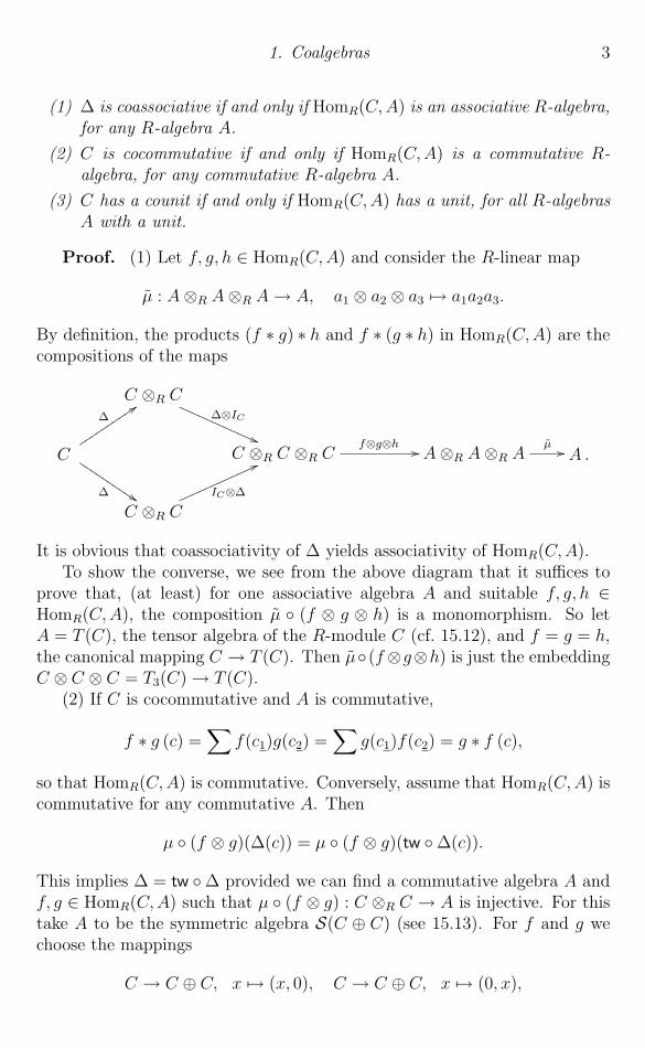
By definition, the products (f ∗ g) ∗ h and f ∗ (g ∗ h) in HomR(C,A) are thecompositions of the maps
C ⊗R C∆⊗IC
�������
������
�
C
∆������������
∆ �������
�����
C ⊗R C ⊗R Cf⊗g⊗h �� A⊗R A⊗R A
µ �� A .
C ⊗R CIC⊗∆
��������������
It is obvious that coassociativity of ∆ yields associativity of HomR(C,A).To show the converse, we see from the above diagram that it suffices to
prove that, (at least) for one associative algebra A and suitable f, g, h ∈HomR(C,A), the composition µ ◦ (f ⊗ g ⊗ h) is a monomorphism. So letA = T (C), the tensor algebra of the R-module C (cf. 15.12), and f = g = h,the canonical mapping C → T (C). Then µ◦ (f⊗g⊗h) is just the embeddingC ⊗ C ⊗ C = T3(C)→ T (C).
(2) If C is cocommutative and A is commutative,
f ∗ g (c) =∑
f(c1)g(c2) =∑
g(c1)f(c2) = g ∗ f (c),
so that HomR(C,A) is commutative. Conversely, assume that HomR(C,A) iscommutative for any commutative A. Then
µ ◦ (f ⊗ g)(∆(c)) = µ ◦ (f ⊗ g)(tw ◦∆(c)).
This implies ∆ = tw ◦∆ provided we can find a commutative algebra A andf, g ∈ HomR(C,A) such that µ ◦ (f ⊗ g) : C ⊗R C → A is injective. For thistake A to be the symmetric algebra S(C ⊕ C) (see 15.13). For f and g wechoose the mappings
C → C ⊕ C, x �→ (x, 0), C → C ⊕ C, x �→ (0, x),

4 Chapter 1. Coalgebras and comodules
composed with the canonical embedding C ⊕ C → S(C ⊕ C).With the canonical isomorphism h : S(C)⊗S(C)→ S(C⊕C) (see 15.13)
and the embedding λ : C → S(C), we form h−1 ◦ µ ◦ (f ⊗ g) = λ⊗ λ. Sinceλ(C) is a direct summand of S(C), we obtain that λ ⊗ λ is injective and soµ ◦ (f ⊗ g) is injective.
(3) It is easy to check that the unit in HomR(C,A) is
Cε−→ R
ι−→ A, c �→ ε(c)1A.
For the converse, consider the R-module A = R ⊕ C and define a unitalR-algebra
µ : A⊗R A→ A, (r, a)⊗ (s, b) �→ (rs, rb+ as).
Suppose there is a unit element in HomR(C,A),
e : C → A = R⊕ C, c �→ (ε(c), λ(c)),
with R-linear maps ε : C → R, λ : C → C. Then, for f : C → A, c �→ (0, c),multiplication in HomR(C,A) yields
f ∗ e : C → A, c �→ (0, (IC ⊗ ε) ◦∆(c)).
By assumption, f = f ∗ e and hence IC = (IC ⊗ ε) ◦∆, one of the conditionsfor ε to be a counit. Similarly, the other condition is derived from f = e ∗ f .
Clearly ε is the unit in HomR(C,R), showing the uniqueness of a counitfor C. �
Note in particular that C∗ = HomR(C,R) is an algebra with the convolu-tion product known as the dual or convolution algebra of C.
Notation. From now on, C (usually) will denote a coassociative R-coalgebra(C,∆, ε), and A will stand for an associative R-algebra with unit (A, µ, ι).
Many properties of coalgebras depend on properties of the base ring R.The base ring can be changed in the following way.
1.4. Scalar extension. Let C be an R-coalgebra and S an associative com-mutative R-algebra with unit. Then C ⊗R S is an S-coalgebra with the co-product
∆ : C ⊗R S∆⊗IS �� (C ⊗R C)⊗R S � �� (C ⊗R S)⊗S (C ⊗R S)
and the counit ε⊗ IS : C ⊗R S → S. If C is cocommutative, then C ⊗R S iscocommutative.

1. Coalgebras 5
Proof. By definition, for any c⊗ s ∈ C ⊗R S,
∆(c⊗ s) =∑(c1 ⊗ 1S)⊗S (c2 ⊗ s).
It is easily checked that ∆ is coassociative. Moreover,
(ε⊗ IS ⊗ IC⊗RS) ◦ ∆(c⊗ s) =∑
ε(c1)c2 ⊗ s = c⊗ s,
and similarly (IC⊗RS ⊗ ε⊗ IS) ◦ ∆ = IC⊗RS is shown.Obviously cocommutativity of ∆ implies cocommutativity of ∆. � To illustrate the notions introduced above we consider some examples.
1.5. R as a coalgebra. The ring R is (trivially) a coassociative, cocommu-tative coalgebra with the canonical isomorphism R → R ⊗R R as coproductand the identity map R→ R as counit.
1.6. Free modules as coalgebras. Let F be a free R-module with basis(fλ)Λ, Λ any set. Then there is a unique R-linear map
∆ : F → F ⊗R F, fλ �→ fλ ⊗ fλ,
defining a coassociative and cocommutative coproduct on F . The counit isprovided by the linear map ε : F → R, fλ �−→ 1.
1.7. Semigroup coalgebra. Let G be a semigroup. A coproduct and couniton the semigroup ring R[G] can be defined by
∆1 : R[G]→ R[G]⊗R R[G], g �→ g ⊗ g, ε1 : R[G]→ R, g �→ 1.
If G has a unit e, then another possibility is
∆2 : R[G]→ R[G]⊗R R[G], g �→{e⊗ e if g = e,g ⊗ e+ e⊗ g if g �= e.
ε2 : R[G]→ R, g �→{1 if g = e,0 if g �= e.
Both ∆1 and ∆2 are coassociative and cocommutative.
1.8. Polynomial coalgebra. A coproduct and counit on the polynomialring R[X] can be defined as algebra homomorphisms by
∆1 : R[X]→ R[X]⊗R R[X], X i �→ X i ⊗X i,
ε1 : R[X]→ R, X i �→ 1, i = 0, 1, 2, . . . .
or else by
∆2 : R[X]→ R[X]⊗R R[X], 1 �→ 1, X i �→ (X ⊗ 1 + 1⊗X)i,
ε2 : R[X]→ R, 1 �→ 1, X i �→ 0, i = 1, 2, . . . .
Again, both ∆1 and ∆2 are coassociative and cocommutative.

6 Chapter 1. Coalgebras and comodules
1.9. Coalgebra of a projective module. Let P be a finitely generatedprojective R-module with dual basis p1, . . . , pn ∈ P and π1, . . . , πn ∈ P ∗.There is an isomorphism
P ⊗R P ∗ → EndR(P ), p⊗ f �→ [a �→ f(a)p],
and on P ∗ ⊗R P the coproduct and counit are defined by
∆ : P ∗ ⊗R P → (P ∗ ⊗R P )⊗R (P ∗ ⊗R P ), f ⊗ p �→∑i
f ⊗ pi ⊗ πi ⊗ p,
ε : P ∗ ⊗R P → R, f ⊗ p �→ f(p).
By properties of the dual basis,
(IP⊗RP ∗ ⊗ ε)∆(f ⊗ p) =∑i
f ⊗ piπi(p) = f ⊗ p,
showing that ε is a counit, and coassociativity of ∆ is proved by the equality
(IP⊗RP ∗⊗∆)∆(f⊗p) =∑
i,jf⊗pi⊗πi⊗pj⊗πj⊗p = (∆⊗IP⊗RP ∗)∆(f⊗p).
The dual algebra of P ∗ ⊗R P is (anti)isomorphic to EndR(P ) by the bi-jective maps
(P ∗ ⊗R P )∗ = HomR(P ∗ ⊗R P,R) � HomR(P, P∗∗) � EndR(P ),
which yield a ring isomorphism or anti-isomorphism, depending from whichside the morphisms are acting.
For P = R we obtain R = R∗, and R∗ ⊗R R � R is the trivial coalgebra.As a more interesting special case we may consider P = Rn. Then P ∗ ⊗R Pcan be identified with the matrix ring Mn(R), and this leads to the
1.10. Matrix coalgebra. Let {eij}1≤i,j≤n be the canonical R-basis forMn(R), and define the coproduct and counit
∆ :Mn(R)→Mn(R)⊗RMn(R), eij �→∑
keik ⊗ ekj,
ε :Mn(R)→ R, eij �→ δij .
The resulting coalgebra is called the (n, n)-matrix coalgebra over R, and wedenote it by M c
n(R).
Notice that the matrix coalgebra may also be considered as a special caseof a semigroup coalgebra in 1.7.
From a given coalgebra one can construct the

1. Coalgebras 7
1.11. Opposite coalgebra. Let ∆ : C → C ⊗R C define a coalgebra. Then
∆tw : C∆−→ C ⊗R C
tw−→ C ⊗R C, c �→∑
c2 ⊗ c1,
where tw is the twist map, defines a new coalgebra structure on C knownas the opposite coalgebra with the same counit. The opposite coalgebra isdenoted by Ccop. Note that a coalgebra C is cocommutative if and only if Ccoincides with its opposite coalgebra (i.e., ∆ = ∆tw).
1.12. Duals of algebras. Let (A, µ, ι) be an R-algebra and assume RA tobe finitely generated and projective. Then there is an isomorphism
A∗ ⊗R A∗ → (A⊗R A)∗, f ⊗ g �→ [a⊗ b �→ f(a)g(b)],
and the functor HomR(−, R) = (−)∗ yields a coproduct
µ∗ : A∗ → (A⊗R A)∗ � A∗ ⊗R A∗
and a counit (as the dual of the unit of A)
ε := ι∗ : A∗ → R, f �→ f(1A).
This makes A∗ an R-coalgebra that is cocommutative provided µ is commu-tative. If RA is not finitely generated and projective, the above constructiondoes not work. However, under certain conditions the finite dual of A has acoalgebra structure (see 5.7).
Further examples of coalgebras are the tensor algebra 15.12, the symmet-ric algebra 15.13, and the exterior algebra 15.14 of any R-module, and theenveloping algebra of any Lie algebra.
1.13. ExercisesLetM c
n(R) be a matrix coalgebra with basis {eij}1≤i,j≤n (see 1.10). Prove thatthe dual algebra M c
n(R)∗ is an (n, n)-matrix algebra.
(Hint: Consider the basis of M∗ dual to {eij}1≤i,j≤n.)
References. Abuhlail, Gomez-Torrecillas and Wisbauer [50]; Bourbaki[5]; Sweedler [45]; Wisbauer [210].

8 Chapter 1. Coalgebras and comodules
2 Coalgebra morphisms
To discuss coalgebras formally, one would like to understand not only isolatedcoalgebras, but also coalgebras in relation to other coalgebras. In a word, onewould like to view coalgebras as objects in a category.1 For this one needsthe notion of a coalgebra morphism. Such a morphism can be defined as anR-linear map between coalgebras that respects the coalgebra structures (co-products and counits). The idea behind this definition is of course borrowedfrom the idea of an algebra morphism as a map respecting the algebra struc-tures. Once such morphisms are introduced, relationships between coalgebrascan be studied. In particular, we can introduce the notions of a subcoalgebraand a quotient coalgebra. These are the topics of the present section.
2.1. Coalgebra morphisms. Given R-coalgebras C and C ′, an R-linearmap f : C → C ′ is said to be a coalgebra morphism provided the diagrams
Cf ��
∆��
C ′
∆′��
C ⊗R Cf⊗f �� C ′ ⊗R C ′ ,
Cf ��
���
������
�� C ′
ε′��R
are commutative. Explicitly, this means that
∆′ ◦ f = (f ⊗ f) ◦∆, and ε′ ◦ f = ε,
that is, for all c ∈ C,∑f(c1)⊗ f(c2) =
∑f(c)1 ⊗ f(c)2, and ε′(f(c)) = ε(c).
Given an R-coalgebra C and an S-coalgebra D, where S is a commuta-tive ring, a coalgebra morphism between C and D is defined as a pair (α, γ)consisting of a ring morphism α : R → S and an R-linear map γ : C → Dsuch that
γ′ : C ⊗R S → D, c⊗ s �→ γ(c)s,
is an S-coalgebra morphism. Here we consider D as an R-module (inducedby α) and C ⊗R S is the scalar extension of C (see 1.4).
As shown in 1.3, for an R-algebra A, the contravariant functor HomR(−, A)turns coalgebras to algebras. It also turns coalgebra morphisms into algebramorphisms.
1The reader not familiar with category theory is referred to the Appendix, §38.

2. Coalgebra morphisms 9
2.2. Duals of coalgebra morphisms. For R-coalgebras C and C ′, anR-linear map f : C → C ′ is a coalgebra morphism if and only if
Hom(f, A) : HomR(C′, A)→ HomR(C,A)
is an algebra morphism, for any R-algebra A.
Proof. Let f be a coalgebra morphism. Putting f ∗ = HomR(f, A), wecompute for g, h ∈ HomR(C ′, A)
f ∗(g ∗ h) = µ ◦ (g ⊗ h) ◦∆′ ◦ f = µ ◦ (g ⊗ h) ◦ (f ⊗ f) ◦∆= (g ◦ f) ∗ (h ◦ f) = f∗(g) ∗ f ∗(h).
To show the converse, assume that f ∗ is an algebra morphism, that is,
µ ◦ (g ⊗ h) ◦∆′ ◦ f = µ ◦ (g ⊗ h) ◦ (f ⊗ f) ◦∆,
for any R-algebra A and g, h ∈ HomR(C′, A). Choose A to be the tensor
algebra T (C) of the R-module C and choose g, h to be the canonical em-bedding C → T (C) (see 15.12). Then µ ◦ (g ⊗ h) is just the embeddingC ⊗R C → T2(C)→ T (C), and the above equality implies
∆′ ◦ f = (f ⊗ f) ◦∆,
showing that f is a coalgebra morphism. �
2.3. Coideals. The problem of determining which R-submodules of C arekernels of a coalgebra map f : C → C ′ is related to the problem of describingthe kernel of f ⊗ f (in the category of R-modulesMR). If f is surjective, weknow that Ke (f ⊗ f) is the sum of the canonical images of Ke f ⊗R C andC ⊗R Ke f in C ⊗R C (see 40.15). This suggests the following definition.
The kernel of a surjective coalgebra morphism f : C → C ′ is called acoideal of C.
2.4. Properties of coideals. For an R-submodule K ⊂ C and the canonicalprojection p : C → C/K, the following are equivalent:
(a) K is a coideal;
(b) C/K is a coalgebra and p is a coalgebra morphism;
(c) ∆(K) ⊂ Ke (p⊗ p) and ε(K) = 0.
If K ⊂ C is C-pure, then (c) is equivalent to:
(d) ∆(K) ⊂ C ⊗R K +K ⊗R C and ε(K) = 0.
If (a) holds, then C/K is cocommutative provided C is also.

10 Chapter 1. Coalgebras and comodules
Proof. (a) ⇔ (b) is obvious.(b) ⇒ (c) There is a commutative exact diagram
0 �� K ��
��
Cp ��
∆
��
C/K
∆��
��
��
0
0 �� Ke (p⊗ p) �� C ⊗R Cp⊗p �� C/K ⊗R C/K �� 0,
where commutativity of the right square implies the existence of a morphismK → Ke (p⊗p), thus showing ∆(K) ⊂ Ke (p⊗p). For the counit ε : C/K →R of C/K, ε ◦ p = ε and hence ε(K) = 0
(c) ⇒ (b) Under the given conditions, the left-hand square in the abovediagram is commutative and the cokernel property of p implies the existenceof ∆. This makes C/K a coalgebra with the properties required.
(c) ⇔ (d) If K ⊂ C is C-pure, Ke (p⊗ p) = C ⊗R K +K ⊗R C. �
2.5. Factorisation theorem. Let f : C → C ′ be a morphism of R-coalgebras. If K ⊂ C is a coideal and K ⊂ Ke f , then there is a commutativediagram of coalgebra morphisms
Cp ��
f ���
����
��C/K
f
��C ′ .
Proof. Denote by f : C/K → C ′ the R-module factorisation of f : C →C ′. It is easy to show that the diagram
C/Kf ��
∆��
C ′
∆′��
C/K ⊗R C/Kf⊗f �� C ′ ⊗R C ′
is commutative. This means that f is a coalgebra morphism. �
2.6. The counit as a coalgebra morphism. View R as a trivial R-coalgebra as in 1.5. Then, for any R-coalgebra C,
(1) ε is a coalgebra morphism;
(2) if ε is surjective, then Ke ε is a coideal.
Proof. (1) Consider the diagram
Cε ��
∆
��
R
���
c � ��
��
ε(c)
��C ⊗R C
ε⊗ε �� R⊗R R∑c1 ⊗ c2
� ��∑ε(c1)⊗ ε(c2) .

2. Coalgebra morphisms 11
The properties of the counit yield∑ε(c1)⊗ ε(c2) =
∑ε(c1)ε(c2)⊗ 1 = ε(
∑c1ε(c2))⊗ 1 = ε(c)⊗ 1,
so the above diagram is commutative and ε is a coalgebra morphism.(2)This is clear by (1) and the definition of coideals. �
2.7. Subcoalgebras. An R-submodule D of a coalgebra C is called a sub-coalgebra provided D has a coalgebra structure such that the inclusion mapis a coalgebra morphism.
Notice that a pure R-submodule (see 40.13 for a discussion of purity) D ⊂C is a subcoalgebra provided ∆D(D) ⊂ D⊗RD ⊂ C ⊗R C and ε|D : D → Ris a counit for D. Indeed, since D is a pure submodule of C, we obtain
∆D(D) = D ⊗R C ∩ C ⊗R D = D ⊗R D ⊂ C ⊗R C,
so that D has a coalgebra structure for which the inclusion is a coalgebramorphism, as required.
From the above observations we obtain:
2.8. Image of coalgebra morphisms. The image of any coalgebra mapf : C → C ′ is a subcoalgebra of C ′.
2.9. Remarks. (1) In a general categoryA, subobjects of an object A inA aredefined as equivalence classes of monomorphisms D → A. In the definitionof subcoalgebras we restrict ourselves to subsets (or inclusions) of an object.This will be general enough for our purposes.
(2) The fact that – over arbitrary rings – the tensor product of injectivelinear maps need not be injective leads to some unexpected phenomena. Forexample, a submodule D of a coalgebra C can have two distinct coalgebrastructures such that, for both of them, the inclusion is a coalgebra map (seeExercise 2.15(3)). It may also happen that, for a submodule V of a coalgebraC, ∆(V ) is contained in the image of the canonical map V ⊗R V → C ⊗R C,yet V has no coalgebra structure for which the inclusion V → C is a coalgebramap (see Exercise 2.15(4)). Another curiosity is that the kernel of a coalgebramorphism f : C → C ′ need not be a coideal in case f is not surjective (seeExercise 2.15(5)).
2.10. Coproduct of coalgebras. For a family {Cλ}Λ of R-coalgebras, putC =
⊕ΛCλ, the coproduct inMR, iλ : Cλ → C the canonical inclusions, and
consider the R-linear maps
Cλ∆λ−→ Cλ ⊗ Cλ ⊂ C ⊗ C, ε : Cλ → R.
By the properties of coproducts of R-modules there exist unique maps

12 Chapter 1. Coalgebras and comodules
∆ : C → C ⊗R C with ∆ ◦ iλ = ∆λ, ε : C → R with ε ◦ iλ = ελ.
(C,∆, ε) is called the coproduct (or direct sum) of the coalgebras Cλ. It isobvious that the iλ : Cλ → C are coalgebra morphisms.
C is coassociative (cocommutative) if and only if all the Cλ have thecorresponding property. This follows – by 1.3 – from the ring isomorphism
HomR(C,A) = HomR(⊕
ΛCλ, A) �∏
ΛHomR(Cλ, A),
for any R-algebra A, and the observation that the left-hand side is an asso-ciative (commutative) ring if and only if every component in the right-handside has this property.
Universal property of C =⊕
ΛCλ. For a family {fλ : Cλ → C ′}Λ of coal-gebra morphisms there exists a unique coalgebra morphism f : C → C ′ suchthat, for all λ ∈ Λ, there are commutative diagrams of coalgebra morphisms
Cλiλ ��
fλ
C
f
��C ′ .
2.11. Direct limits of coalgebras. Let {Cλ, fλµ}Λ be a direct family of R-coalgebras (with coalgebra morphisms fλµ) over a directed set Λ. Let lim−→Cλdenote the direct limit in MR with canonical maps fµ : Cµ → lim−→Cλ. Thenthe fλµ⊗ fλµ : Cλ⊗Cλ → Cµ⊗Cµ form a directed system (inMR) and thereis the following commutative diagram
Cµ∆µ ��
fµ��
Cµ ⊗ Cµ
��
fµ⊗fµ���
��������
���
lim−→Cλδ �� lim−→(Cλ ⊗ Cλ)
θ �� lim−→Cλ ⊗ lim−→Cλ,
where the maps δ and θ exist by the universal properties of direct limits. Thecomposition
∆lim = θ ◦ δ : lim−→Cλ → lim−→Cλ ⊗ lim−→Cλ
turns lim−→Cλ into a coalgebra such that the canonical map (e.g., [46, 24.2])
p :⊕
ΛCλ → lim−→Cλ
is a coalgebra morphism. The counit of lim−→Cλ is the map εlim determined bythe commutativity of the diagrams
Cµfµ ��
���
����
����
lim−→Cλ
εlim
��R .

2. Coalgebra morphisms 13
For any associative R-algebra A,
HomR(lim−→Cλ, A) � lim←−HomR(Cλ, A) ⊂∏
ΛHomR(Cλ, A),
and from this we conclude – by 1.3 – that the coalgebra lim−→Cλ is coassociative(cocommutative) whenever all the Cλ are coassociative (cocommutative).
Recall that for the definition of the tensor product of R-algebras A,B, thetwist map tw : A⊗R B → B ⊗R A, a⊗ b �→ b⊗ a is needed. It also helps todefine the
2.12. Tensor product of coalgebras. Let C and D be two R-coalgebras.Then the composite map
C ⊗R D∆C⊗∆D�� (C ⊗R C)⊗R (D ⊗R D)
IC⊗tw⊗ID �� (C ⊗R D)⊗R (C ⊗R D)
defines a coassociative coproduct on C ⊗R D, and with the counits εC of Cand εD of D the map εC⊗εD : C⊗RD → R is a counit of C⊗RD. With thesemaps, C ⊗R D is called the tensor product coalgebra of C and D. ObviouslyC ⊗R D is cocommutative provided both C and D are cocommutative.
2.13. Tensor product of coalgebra morphisms. Let f : C → C ′ andg : D → D′ be morphisms of R-coalgebras. The tensor product of f and gyields a coalgebra morphism
f ⊗ g : C ⊗R D → C ′ ⊗R D′.
In particular, there are coalgebra morphisms
IC ⊗ εD : C ⊗R D → C, εC ⊗ ID : C ⊗R D → D,
which, for any commutative R-algebra A, lead to an algebra morphism
HomR(C,A)⊗R HomR(D,A)→ HomR(C ⊗R D,A),
ξ ⊗ ζ �→ (ξ ◦ (IC ⊗ εD)) ∗ (ζ ◦ (εC ⊗ ID)),
where ∗ denotes the convolution product (cf. 1.3).
Proof. The fact that f and g are coalgebra morphisms implies commu-tativity of the top square in the diagram
C ⊗R Df⊗g ��
∆C⊗∆D
��
C ′ ⊗R D′
∆C′⊗∆D′��
C ⊗R C ⊗R D ⊗R Df⊗f⊗g⊗g ��
IC⊗tw⊗ID��
C ′ ⊗R C ′ ⊗R D′ ⊗R D′
IC′⊗tw⊗ID′��
C ⊗R D ⊗R C ⊗R Df⊗g⊗f⊗g �� C ′ ⊗R D′ ⊗R C ′ ⊗R D′ ,

14 Chapter 1. Coalgebras and comodules
while the bottom square obviously is commutative by the definitions. Com-mutativity of the outer rectangle means that f ⊗ g is a coalgebra morphism.
By 2.2, the coalgebra morphisms C ⊗R D → C and C ⊗R D → D yieldalgebra maps
HomR(C,A)→ HomR(C ⊗R D,A), HomR(D,A)→ HomR(C ⊗R D,A) ,
and with the product in HomR(C ⊗R D,A) we obtain a map
HomR(C,A)× HomR(D,A)→ HomR(C ⊗R D,A),
which is R-linear and hence factorises over HomR(C,A)⊗RHomR(D,A). Thisis in fact an algebra morphism since the image of HomR(C,A) commutes withthe image of HomR(D,A) by the equalities
((ξ ◦ (IC ⊗ εD)) ∗ (ζ ◦ (εC ⊗ ID)))(c⊗ d)=
∑ξ ◦ (IC ⊗ εD)⊗ ζ ◦ (εC ⊗ ID)(c1 ⊗ d1 ⊗ c2 ⊗ d2)
=∑
ξ(c1ε(d1)) ζ(ε(c2)d2)
=∑
ξ(c1ε(c2), ζ(ε(d1)d2)
= ξ(c) ζ(d) = ζ(d) ξ(c)
= ((ζ ◦ (εC ⊗ ID)) ∗ (ξ ◦ (IC ⊗ εD)))(c⊗ d),
where ξ ∈ HomR(C,A), ζ ∈ HomR(D,A) and c ∈ C, d ∈ D. �
To define the comultiplication for the tensor product of two R-coalgebrasC,D in 2.12, the twist map tw : C ⊗R D → D ⊗R C was used. Notice thatany such map yields a formal comultiplication on C ⊗R D, whose propertiesstrongly depend on the properties of the map chosen.
2.14. Coalgebra structure on the tensor product. For R-coalgebras(C,∆C , εC) and (D,∆D, εD), let ω : C ⊗R D → D⊗R C be an R-linear map.Explicitly on elements we write ω(c⊗ d) =
∑dω ⊗ cω. Denote by C�ωD the
R-module C ⊗R D endowed with the maps
∆ = (IC ⊗ ω ⊗ ID) ◦ (∆C ⊗∆D) : C ⊗R D → (C ⊗R D)⊗R (C ⊗R D),ε = εC ⊗ εD : C ⊗R D → R.
Then C�ωD is an R-coalgebra if and only if the following bow-tie diagram
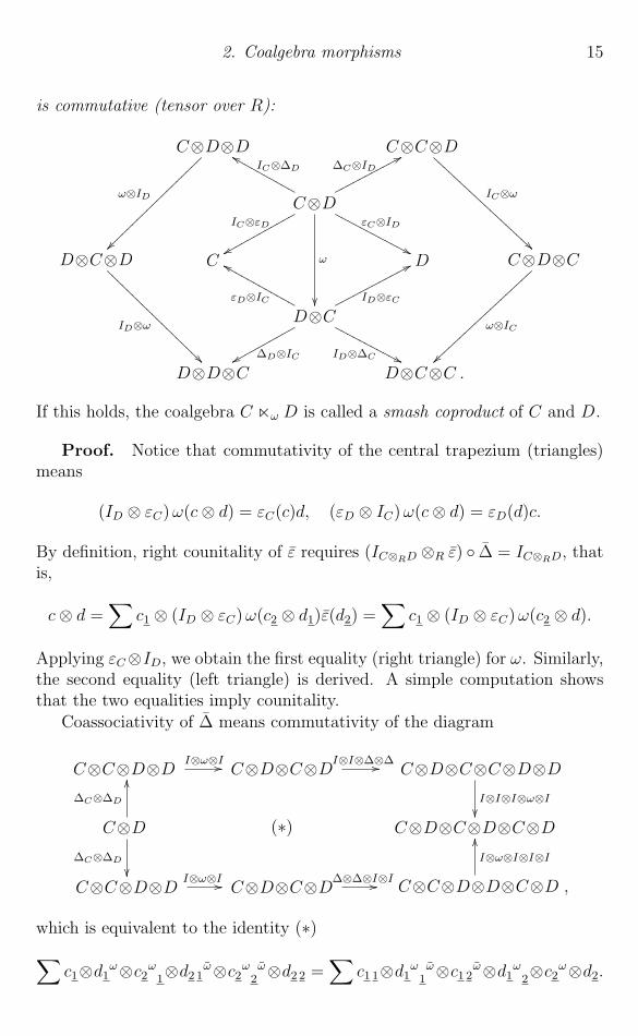
2. Coalgebra morphisms 15
is commutative (tensor over R):
C⊗D⊗D
ω⊗ID
��
C⊗C⊗D
IC⊗ω
�����
����
����
����
����
C⊗D
∆C⊗ID �����������
IC⊗∆D
������������
εC⊗ID
�������
������
�
ω
��
IC⊗εD
��������
������
D⊗C⊗D
ID⊗ω
�����
����
����
����
����
C D C⊗D⊗C
ω⊗IC
���������������������
D⊗CID⊗εC
������������εD⊗IC
��������������
ID⊗∆C �������
������
∆D⊗IC��������
����
D⊗D⊗C D⊗C⊗C .
If this holds, the coalgebra C �ω D is called a smash coproduct of C and D.
Proof. Notice that commutativity of the central trapezium (triangles)means
(ID ⊗ εC)ω(c⊗ d) = εC(c)d, (εD ⊗ IC)ω(c⊗ d) = εD(d)c.
By definition, right counitality of ε requires (IC⊗RD ⊗R ε) ◦ ∆ = IC⊗RD, thatis,
c⊗ d =∑
c1 ⊗ (ID ⊗ εC)ω(c2 ⊗ d1)ε(d2) =∑
c1 ⊗ (ID ⊗ εC)ω(c2 ⊗ d).
Applying εC⊗ID, we obtain the first equality (right triangle) for ω. Similarly,the second equality (left triangle) is derived. A simple computation showsthat the two equalities imply counitality.
Coassociativity of ∆ means commutativity of the diagram
C⊗C⊗D⊗D I⊗ω⊗I�� C⊗D⊗C⊗DI⊗I⊗∆⊗∆�� C⊗D⊗C⊗C⊗D⊗DI⊗I⊗I⊗ω⊗I��
C⊗D
∆C⊗∆D
��
∆C⊗∆D
��
(∗) C⊗D⊗C⊗D⊗C⊗D
C⊗C⊗D⊗D I⊗ω⊗I �� C⊗D⊗C⊗D∆⊗∆⊗I⊗I�� C⊗C⊗D⊗D⊗C⊗D ,
I⊗ω⊗I⊗I⊗I��
which is equivalent to the identity (∗)∑c1⊗d1ω⊗c2ω1⊗d2 1
ω⊗c2ω2ω⊗d2 2 =
∑c1 1⊗d1ω1
ω⊗c1 2ω⊗d1ω2⊗c2ω⊗d2.

16 Chapter 1. Coalgebras and comodules
Applying the map εC ⊗ IC ⊗ ID ⊗ ID ⊗ IC ⊗ εD to the last module in thediagram (∗) – or to formula (∗) – we obtain the commutative diagram andformula
C ⊗D ⊗Dω⊗I �� D ⊗ C ⊗D
I⊗∆C⊗I�� D ⊗ C ⊗ C ⊗D
I⊗I⊗ω��
C ⊗D
I⊗∆D
��
∆C⊗I��
(∗∗) D ⊗ C ⊗D ⊗ C
C ⊗ C ⊗DI⊗ω �� C ⊗D ⊗ C
I⊗∆D⊗I�� C ⊗D ⊗D ⊗ C ,
ω⊗I⊗I��
(∗∗)∑
d1ω ⊗ cω1 ⊗ d2
ω ⊗ cω2ω =
∑dω1
ω ⊗ c1ω ⊗ dω2 ⊗ c2
ω.
Now assume formula (∗∗) to be given. Tensoring from the left with thecoefficients c1 and replacing c by the coefficients c2 we obtain∑
c1 ⊗ d1ω ⊗ c2
ω1⊗ d2
ω ⊗ c2ω2ω =
∑c1 ⊗ dω1
ω ⊗ c2 1ω ⊗ dω2 ⊗ c2 2
ω
=∑c1 1 ⊗ dω1
ω ⊗ c1 2ω ⊗ dω2 ⊗ c2
ω.
Now, tensoring with the coefficients d2 from the right and replacing d by thecoefficients d1 we obtain formula (∗). So both conditions (∗∗) and (∗) areequivalent to coassociativity of ∆.
Commutativity of the trapezium yields a commutative diagram
D ⊗ C ⊗ C ⊗D
ID⊗IC⊗ω��
ID⊗εC⊗ω������
����������
�����
D ⊗ C ⊗D ⊗ CID⊗εC⊗ID⊗IC�� D ⊗D ⊗ C .
C ⊗D ⊗D ⊗ C
ω⊗ID⊗IC��
εC⊗ID⊗ID⊗IC
���������������������
With this it is easy to see that the diagram (∗∗) reduces to the diagram
C ⊗D ⊗Dω⊗ID �� D ⊗ C ⊗D
IC⊗ω��
C ⊗Dω ��
IC⊗∆D
��
D ⊗ C∆D⊗IC�� D ⊗D ⊗ C,
and a similar argument with εD ⊗ IC yields the diagram
C ⊗Dω ��
∆C⊗ID��
D ⊗ CID⊗∆C�� D ⊗ C ⊗ C
C ⊗ C ⊗DIC⊗ω �� C ⊗D ⊗ C .
ω⊗IC��

2. Coalgebra morphisms 17
Notice that the two diagrams are the left and right wings of the bow-tie andhence one direction of our assertion is proven.
Commutativity of these diagrams corresponds to the equations∑d1ω⊗d2ω⊗cωω =
∑dω1⊗dω2⊗cω,
∑dω⊗cω1⊗cω2 =
∑dωω⊗c1ω⊗c2ω,
and – alternatively – these can be obtained by applying ID ⊗ εC ⊗ ID ⊗ ICand ID ⊗ IC ⊗ εD ⊗ IC to equation (∗∗).
For the converse implication assume the bow-tie diagram to be commuta-tive. Then the trapezium is commutative and hence ε is a counit. Moreover,the above equalities hold. Tensoring the first one with the coefficients c1 andreplacing c by the coefficients c2 we obtain∑
c1 ⊗ d1ω ⊗ d2
ω ⊗ c2ωω =
∑c1 ⊗ dω1 ⊗ dω2 ⊗ c2
ω.
Applying ω ⊗ ID ⊗ IC to this equation yields∑d1ωω ⊗ c1
ω ⊗ d2ω ⊗ c2
ωω =∑
dω1ω ⊗ c1
ω ⊗ dω2 ⊗ c2ω.
Now, tensoring the second equation with the coefficients d2 from the right,replacing d by the coefficients d1 and then applying ID ⊗ IC ⊗ ω yields∑
d1ω ⊗ cω1 ⊗ d2
ω ⊗ cω2ω =
∑d1ωω ⊗ c1
ω ⊗ d2ω ⊗ c2
ωω.
Comparing the two equations we obtain (∗∗), proving the coassociativity of∆. �
Notice that a dual construction and a dual bow-tie diagram apply forthe definiton of a general product on the tensor product of two R-algebrasA,B by an R-linear map ω′ : B ⊗R A → A ⊗R B. A partially dual bow-tiediagram arises in the study of entwining structures between R-algebras andR-coalgebras (cf. 32.1).
2.15. Exercises
(1) Let g : A → A′ be an R-algebra morphism. Prove that, for any R-coalgebraC,
Hom(C, g) : HomR(C,A)→ HomR(C,A′)
is an R-algebra morphism.(2) Let f : C → C ′ be an R-coalgebra morphism. Prove that, if f is bijective
then f−1 is also a coalgebra morphism.(3) On the Z-module C = Z ⊕ Z/4Z define a coproduct
∆ : C → C ⊗Z C, (1, 0) �→ (1, 0)⊗ (1, 0),(0, 1) �→ (1, 0)⊗ (0, 1) + (0, 1)⊗ (1, 0).

18 Chapter 1. Coalgebras and comodules
On the submodule D = Z ⊕ 2Z/4Z ⊂ C consider the coproducts
∆1 : D → D ⊗Z D, (1, 0) �→ (1, 0)⊗ (1, 0),(0, 2) �→ (1, 0)⊗ (0, 2) + (0, 2)⊗ (1, 0),
∆2 : D → D ⊗Z D, (1, 0) �→ (1, 0)⊗ (1, 0),(0, 2) �→ (1, 0)⊗(0, 2) + (0, 2)⊗(0, 2) + (0, 2)⊗(1, 0).
Prove that (D,∆1) and (D,∆2) are not isomorphic but the canonical inclu-sion D → C is an algebra morphism for both of them (Nichols and Sweedler[168]).
(4) On the Z-module C = Z/8Z ⊕ Z/2Z define a coproduct
∆ : C → C ⊗Z C, (1, 0) �→ 0,(0, 1) �→ 4(1, 0)⊗ (1, 0)
and consider the submodule V = Z(2, 0) + Z(0, 1) ⊂ C. Prove:
(i) ∆ is well defined.(ii) ∆(V ) is contained in the image of V ⊗R V → C ⊗R C.(iii) ∆ : V → C ⊗R C has no lifting to V ⊗R V (check the order of the
preimage of ∆(0, 1) in V ⊗R V ) (Nichols and Sweedler [168]).(5) Let C = Z ⊕ Z/2Z ⊕ Z, denote c0 = (1, 0, 0), c1 = (0, 1, 0), c2 = (0, 0, 1) and
define a coproduct
∆(cn) =n∑i=0
ci ⊗ cn−i, n = 0, 1, 2.
Let D = Z ⊕ Z/4Z, denote d0 = (1, 0), d1 = (0, 1) and
∆(d0) = d0 ⊗ d0, ∆(d1) = d0 ⊗ d1 + d1 ⊗ d0.
Prove that the map
f : C → D, c0 �→ d0, c1 �→ 2d1, c2 �→ 0,
is a Z-coalgebra morphism and ∆(c2) �∈ c2 ⊗ C + C ⊗ c2 (which implies thatKe f = Zc2 is not a coideal in C) (Nichols and Sweedler [168]).
(6) Prove that the tensor product of coalgebras yields the product in the categoryof cocommutative coassociative coalgebras.
(7) Let (C,∆C , εC) and (D,∆D, εD) be R-coalgebras with an R-linear mappingω : C ⊗R D → D ⊗R C. Denote by C�ωD the R-module C ⊗R D endowedwith the maps ∆ and ε as in 2.14. The map ω is said to be left or rightconormal if for any c ∈ C, d ∈ D,
(ID ⊗ εC)ω(c⊗ d) = ε(c)d or (εD ⊗ IC)ω(c⊗ d) = εD(d)c.
Prove:(i) The following are equivalent:

2. Coalgebra morphisms 19
(a) ω is left conormal;(b) εC ⊗ ID : C�ωD → D respects the coproduct;(c) (IC⊗RD ⊗R ε) ◦ ∆ = IC⊗RD.
(ii) The following are equivalent:
(a) ω is right conormal;(b) IC ⊗ εD : C�ωD → C respects the coproduct;(c) (ε⊗R IC⊗RD) ◦ ∆ = IC⊗RD.
References. Caenepeel, Militaru and Zhu [9]; Nichols and Sweedler [168];Sweedler [45]; Wisbauer [210].

20 Chapter 1. Coalgebras and comodules
3 Comodules
In algebra or ring theory, in addition to an algebra, one would also like tostudy its modules, that is, Abelian groups on which the algebra acts. Cor-respondingly, in the coalgebra theory one would like to study R-moduleson which an R-coalgebra C coacts. Such modules are known as (right) C-comodules, and for any given C they form a category MC , provided mor-phisms or C-comodule maps are suitably defined. In this section we definethe category MC and study its properties. The category MC in many re-spects is similar to the category of modules of an algebra, for example, thereare Hom-tensor relations, there exist cokernels, and so on, and indeed thereis a close relationship between MC and the modules of the dual coalgebraC∗ (cf. Section 4). On the other hand, however, there are several markeddifferences between categories of modules and comodules. For example, thecategory of modules is an Abelian category, while the category of comodulesof a coalgebra over a ring might not have kernels (and hence it is not anAbelian category in general). This is an important (lack of) property that ischaracteristic for coalgebras over rings (if R is a field then MC is Abelian),that makes studies of such coalgebras particularly interesting. The ring struc-ture of R and the R-module structure of C play in these studies an importantrole, which requires careful analysis of R-relative properties of a coalgebra orboth C- and R-relative properties of comodules.
As before, R denotes a commutative ring,MR the category of R-modules,and C, more precisely (C,∆, ε), stands for a (coassociative) R-coalgebra (withcounit). We first introduce right comodules over C.
3.1. Right C-comodules. For M ∈ MR, an R-linear map �M : M →M ⊗R C is called a right coaction of C on M or simply a right C-coaction.To denote the action of �M on elements of M we write �M(m) =
∑m0⊗m1.
A C-coaction �M is said to be coassociative and counital provided thediagrams
M�M ��
�M
��
M ⊗R CIM⊗∆��
M ⊗R C�M⊗IC ��M ⊗R C ⊗R C,
M�M ��
IM �������
�����
M ⊗R CIM⊗ε��M
are commutative. Explicitly, this means that, for all m ∈M ,∑�M(m0)⊗m1 =
∑m0 ⊗∆(m1), m =
∑m0ε(m1).
In view of the first of these equations we can shorten the notation and write
(IM ⊗∆) ◦ �M(m) =∑
m0 ⊗m1 ⊗m2,