Corporate Cash Holdings:

An empirical investigation of Portuguese

companies

Augusto Rafael dos Santos Borges

up201400162@fep.up.pt

Dissertation

Master in Finance

Supervisor: Professor Jorge Bento Barbosa Farinha

2016

i

Biographical Note

Augusto Rafael dos Santos Borges was born in Vila Real in 1992. He completed his BSc

in Economics from University of Coimbra in 2014. Throughout his undergraduate

studies, he was involved in several initiatives, he took part in two summer internships and

he was member of AIESEC in Coimbra for over 2 years. In September 2014, he started

his Master course in Finance at School of Economics and Management, University of

Porto, with the goal of studying the areas of corporate finance and financial markets.

Along the second year of the master course, he performed a professional activity in

Planning and Management Control at EDP.

ii

Acknowledgements

I would like to express my gratitude to everyone who directly or indirectly helped me to

achieve this goal. In particular, to my family for their unconditional support, concerns

and encouragement. To my friends, for their help and friendship, and to all of the

professors and staff of the school, who contributed for this achievement. Specially, a huge

thanks to Professor Jorge Farinha, for his expertise, constructive feedback, guidance and

dedication along this work. Without his help this would not be possible. An

extra acknowledgement to Professor Vítor Castro, for his availability and suggestions.

iii

Abstract

Why do firms hold so many liquid assets on their balance sheets? The amount of a firm’s

liquidity depends on its treasury management policy. There are several justifications

regarding possession of liquid assets. The finance literature highlights three theoretical

models that explain how the companies’ characteristics influence the levels of cash, there

are the trade-off, pecking order and free cash flow theories. This study tests the

predictions resulting from several factors that are suggested by the above mentioned

theories. We find that the firm’s growth opportunities, leverage and dividend payments

have positive effects on cash holdings. Additionally, longer debt maturity and cash flow

generated by the firm exert a negative effect. Therefore, it can be concluded that the trade-

off theory best explains the evolution of the liquidity of listed companies in Portugal. We

also find that governance characteristics play an interesting role concerning the levels of

cash. Moreover, we find that the 2008 financial crisis impact on the firms’ cash holdings

and its financial characteristics. In particular, the growth opportunities cease to be

significant in a post-crisis period, while the negative effect of the cash flow generated by

the firm gains significance in the post-crisis period.

Key-words: Cash holdings; Trade-off theory; Pecking order theory; Free cash flow

theory; Corporate governance; Financial crisis of 2008

JEL Classification: G3, G32, G39

iv

Resumo

Por que razão possui uma empresa tantos ativos líquidos no seu balanço? A quantidade

de liquidez de uma empresa depende da sua política de gestão de tesouraria. Existem

diversas justificações para a posse de ativos líquidos. A literatura em finanças destaca três

modelos teóricos que explicam como as características das empresas influenciam no nível

da tesouraria das mesmas, a saber são a teoria de trade-off, a teoria pecking order e a

teoria free cash flow. Este estudo testa as previsões decorrentes dos vários fatores que são

sugeridos pelos modelos anteriores. Concluindo que as oportunidades de crescimento,

alavancagem e pagamento de dividendos da empresa têm efeitos positivos sobre os níveis

de liquidez. Além disso, uma estrutura dívida de longo prazo e fluxo de caixa gerado pela

empresa de exerce um efeito negativo. Assim, pode-se concluir que a teoria de trade-off

é aquela que melhor consegue explicar a evolução da liquidez das empresas cotadas em

Portugal. Concluímos também que as características de governo das empresas

desempenham um papel interessante na gestão de liquidez. Além disso, descobrimos que

a crise financeira de 2008 tem um impacto relevante sobre o nível de liquidez e as suas

características. Em específico, as oportunidades de crescimento deixam de ser fatores

determinantes significativos num período de pós-crise, ao passo que o efeito negativo do

fluxo de caixa gerado pela empresa ganha significância no período pós-crise.

Palavras-chave: Gestão de liquidez; Teoria de trade-off; Teoria pecking order; Teoria

free cash flow; Governo empresarial; Crise financeira de 2008

Classificação JEL: G3, G32, G39

v

Contents

1. Introduction .................................................................................................................. 1

2. Literature Review ......................................................................................................... 3

2.1. Theoretical Motives for Cash Holdings ................................................................. 3

2.2. Cash Holdings Theories ......................................................................................... 4

2.2.1. Trade-off Theory ............................................................................................. 4

2.2.2. Pecking Order Theory ..................................................................................... 7

2.2.3. Free Cash Flow Theory................................................................................... 8

2.3. Ownership and Board Structure ........................................................................... 10

2.3.1. The largest shareholders ................................................................................ 10

2.3.2. Board Structure ............................................................................................. 11

2.4. Empirical Evidence .............................................................................................. 12

3. Hypotheses Development ........................................................................................... 18

4. Data Description ......................................................................................................... 24

4.1 Dependent Variable .............................................................................................. 24

4.2 Independent Variables .......................................................................................... 25

4.3. Descriptive statistics ............................................................................................ 26

4.4. Methodology ........................................................................................................ 27

5. Empirical Results and Analysis .................................................................................. 30

5.1. Basic Empirical Model ........................................................................................ 30

5.2. Alternative Model ................................................................................................ 34

5.3. Robustness Checks............................................................................................... 36

5.4. Pre and Post-Crisis Analyses ............................................................................... 41

6. Conclusions ................................................................................................................ 45

References ...................................................................................................................... 46

Annexes .......................................................................................................................... 50

vi

Index of Tables

Table 1: Summary of models predictions ...................................................................... 10

Table 2: Financial determinants of firms’ cash holdings ............................................... 16

Table 3: Hypotheses summary....................................................................................... 22

Table 4: Additional hypotheses ..................................................................................... 23

Table 5: Descriptive Statistics ....................................................................................... 27

Table 6: Estimation output of equation (4.3.1) .............................................................. 30

Table 7: Estimation output of equation (4.3.2) .............................................................. 34

Table 8: Robustness checks of equation (4.3.1) ............................................................ 38

Table 9: Estimation output of pre-crisis and post-crisis regressions ............................. 42

Table 10: Description of variables ................................................................................. 50

Table 11: Wald test ........................................................................................................ 51

Table 12: Collinearity Statistics..................................................................................... 51

Table 13: Panel tests III ................................................................................................. 51

Table 14: Robustness checks of equation (4.3.2) .......................................................... 52

Table 15: Im, Pesaran and Shin test output I ................................................................. 54

Table 16: Im, Pesaran and Shin test output II ................................................................ 54

Table 17: Alternative model II ...................................................................................... 55

Index of Figures

Figure 1: Optimal holdings of liquid assets. .................................................................... 5

Figure 2: Cash ratio development.................................................................................. 25

1

1. Introduction

Cash is a key asset on a firm’s balance sheets and receives a significant attention not just

from companies, but also investors and financial analysts. In late 2000 the amount of cash

or cash equivalents held by firms in the European Monetary Union (EMU) amounted to

14.8% of their total book value of assets (Ferreira and Vilela, 2004). More recently and

regarding U.S. market, in the year 2006 the average cash-to-assets ratio held by firms

amounted to around 23% (Bates et al., 2009). Why do firms hold large quantities of cash

and cash equivalents?

Some managers argue that the companies with high cash, or cash equivalents levels, allow

them to quickly take advantage of profitable investment opportunities, and avoid extra

financing costs (Mikkelson and Partch, 2003). Actually there are four broadly accepted

motives for cash holdings: transaction, precautionary, the agency and tax motives

(Keynes, 1936; Jensen, 1986; Foley et al., 2007). The finance literature also identifies

three theoretical models that can help to explain which firm characteristics influence cash

holdings decisions. The trade-off theory suggests that firms identify an optimal level of

cash holdings by weighing its costs and benefits (Ferreira and Vilela, 2004). Then, the

pecking order theory (Myers, 1984) introduces the importance of asymmetric

information. In order to minimise it, firms should finance their investments internally.

Lastly, the free cash flow theory (Jensen, 1986) suggests that managers have incentives

to accumulate large amounts of cash, in order to reduce pressure to improve their

performance.

Many authors have studied important aspects of corporate cash holdings. Kim et al.

(1998), Opler et al. (1999), Mikkelson and Partch (2003) and Bates et al. (2009) all

present studies concerning U.S. firms. In contrast, Ferreira and Vilela (2004) focus in

EMU firms’ while Ozkan and Ozkan (2004) analyse UK firms. In addition Drobetz and

Grüninger (2007) study the case of Swiss firms and Teruel and Solano (2008) investigate

the case of small and medium-size enterprises in Spain, among other studies.

In this research, we examine the empirical characteristics of cash holdings, by testing

factors that have been proposed by previous authors. We focus on factors related to

financial characteristics, and we also perform a sensitivity analysis concerning the

governance data. The research sample is composed by 43 firms and comprises data over

2

the period between 1995 and 2015. Considering the absence of studies examining the

determinants of cash holdings of Portuguese listed firms over the period of financial

crisis, it may be also interesting to explore the effect of the financial crisis on the

determining factors for cash holdings. However, the main goal of this research is to study

the effects of the determining factors associated to the trade-off, pecking order and free

cash flow theories for corporate cash holdings of Portuguese listed firms.

The main findings of our study are the positive and significant association between cash

holdings and growth opportunities, leverage and dividend payments, while long debt

maturity and cash flow generated by the firms exert a negative effect. Hence, it can be

concluded that the trade-off theory collects the strongest support. In contrast, the model

with least support is the free cash flow theory. In addition, we also conclude that

governance factors could play an interesting role concerning cash levels. Moreover, we

find that the financial crisis of 2008 influenced on the relation between cash levels of

Portuguese firms and its determining factors. Specifically, the growth opportunities cease

to be significant in a post-crisis period, while the negative effect of the cash flow

generated by the firm gains significance in the post-crisis period.

The structure of this study will proceed as follows. The second section presents the

literature review, which presents the main motives for cash holdings, the main theories

and introduces some governance issues that could influence on cash levels. In addition,

the second section also includes the empirical findings of similar studies. The third section

presents our hypotheses. In the fourth section, we describe the data and the methodology

adopted in the empirical phase. The fifth section presents the results and its analysis.

Finally, in section 6, we discuss the findings and suggestions for further research.

3

2. Literature Review

The following section is divided into four different subsections. The first one explains the

main motives for cash holdings, the second states the three theoretical models concerning

corporate cash holdings and their determinant factors most accepted by the literature in

finance. The third section introduces some issues regarding corporate governance and

cash holdings. The last section presents the main results of similar studies.

2.1. Theoretical Motives for Cash Holdings

Safeguarding that a firm has adequate liquid assets to finance their future projects is at

the heart of the practice of financial management1. Excess cash, is typically defined as

cash and marketable securities above that used in the normal course of the business (Lins,

et al., 2010). Founded on the assumption of perfect financial markets, assuming no

transaction costs, taxes, asymmetric information and bankruptcy costs, the capital

structure does not affect firm value. Thus, there would be no reason for a company to

hold liquid assets. In case of necessity, requesting a loan from a bank would be enough,

thus companies’ financial decisions would not affect their value (Modigliani and Miller,

1958; Stiglitz, 1974)2. However, there are market imperfections which imply different

motives for corporate cash holdings. The theory of demand for money by firms (Keynes,

1936) and the agency theory (Jensen, 1986) clarify why a firm would choose to hold cash.

According to Keynes (1936) there are two major motives for corporate cash holdings: the

transaction costs and precautionary motives. The transaction costs motive states that a

firm benefits from holding liquid assets because these provide a way to save on

transaction costs: (i) the cost of raising external finance; (ii) the cost of liquidating assets.

The precautionary motive, highlights the importance of anticipating future necessities and

investment opportunities. Thus, precautionary cash holdings seek to self-insure against

costly or unavailable external finance and provide financing in case of investment

opportunities. In recent years, many authors add findings about precautionary cash

holdings. Ferreira and Vilela (2004) find a negative association between the level of

1 Cash holdings are usually defined as cash and marketable securities, or cash and cash equivalents (Opler

et al., 1999). 2 The Modigliani and Miller theorem suggests that the value of an unleveraged firm is equals the value of

a leverage firm (Modigliani and Miller, 1958).

4

capital markets development and cash holdings, which supports the precautionary

motives for cash holdings. In addition, Almeida et al. (2004) study the relation of the

cash’s accumulation according the precautionary motive and the presence of financial

constraints. Their results suggest that constrained firms tend to increase their liquid assets.

Bates et al., (2009) also suggest that firms accumulate cash to face unexpected financial

crisis.

The agency theory (Jensen, 1986) also offers a possible explanation for firms’ cash

holdings. In the presence of agency conflicts between managers and shareholders, such

as asymmetric information or incomplete contracts, managers tend to accumulate cash in

order to proceed with their strategies. Dittmar et al. (2003) empathize the importance of

the agency problem as a deterministic factor that influences cash holdings. Diitmar et al.

(2007) highlight the effect of governance on the value of excess cash, they find that “the

value of a dollar of cash is substantially less if a firm has poor corporate governance”

(Dittmar et al., 2007, p. 627). In addition, they also find that entrenched managers are

more likely to accumulate cash.

A fourth reason for holding liquidity is connected with a tax system motive. Multinational

companies may collect cash in foreign subsidiaries to avoid the repatriation tax expense

they would suffer if they were to repatriate the profits earned in foreign jurisdictions

(Foley et al., 2007).

Founded on the previous motives, the level of cash holdings of a firm is the result of a

balance between the costs and benefits of liquidity and of also of the interests of all

stakeholders.

2.2. Cash Holdings Theories

The corporate cash holdings characteristics are usually explained on the basis of three

theories: the Trade-off, Pecking Order and Free Cash Flow Theories. In order to clarify

the rationale behind each theory and to easily review the predictions by each one, we will

follow the structure proposed by Ferreira and Vilela (2004).

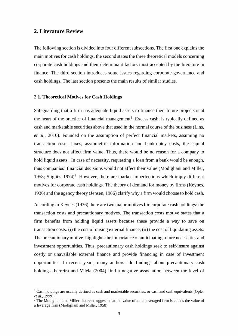
2.2.1. Trade-off Theory

According to the trade-off theory, firms tend to establish an optimal cash level and in

order to reach that, they weigh the cash holdings’ benefits and the cash holdings’ costs

5

(Opler et al., 1999; Ferreira and Vilela, 2004). Assuming that a manager’s goal is to

maximize the shareholders’ wealth, they will set the firm’s cash holdings in a way that

the marginal benefits equal the marginal cost of holding cash. The optimal amount of cash

is given by the intersection of the marginal cost of liquid assets curve and the marginal

cost of liquid asset shortage curve.

Figure 1: Optimal holdings of liquid assets.

Source: Opler et al. (1999)

Note: Figure 1 shows, under Opler et al. (1999) assumptions, that the amount of liquid assets is given by

the intersection of the marginal cost of liquid assets and the marginal cost of liquid asset shortage curves.

The marginal cost curve of being short of liquid assets is downward sloping and the marginal cost curve of

holding liquid assets is assumed to be horizontal. “With the transaction costs model, the cost of liquid assets

is their lower pecuniary expected return, because part of the benefit from holding liquid assets is that they

can be more easily converted into cash. There is no reason to think that this cost varies with the amount of

liquid assets held. If the firm has a shortage of liquid assets, it can cope with the shortage by either

decreasing investment or dividends, or by raising outside funds through security issuances or asset sales.

A greater shortage has greater costs, because addressing a larger shortage involves decreasing investment

more or raising more outside funds” (Opler et al., 1999, p. 8)

Ferreira and Vilela (2004) suggest that the benefits of holding cash include a reduction of

the likelihood of financial distress through the fact that cash holdings (i) act as a buffer

against unexpected losses, (ii) minimize the costs of raising external funds and (iii)

minimize the risks associated with the sale of company’s assets in order to maintain the

investment policy in case of financial distress. On the other hand, the main cash holding’s

cost is the opportunity cost associated to the low return of liquid assets. In addition,

agency problems between the management team and shareholders may be exacerbated

when cash levels are high (Opler et al., 1999). According to the trade-off theory, firms

6

reach their own optimal level of cash holdings when the marginal benefit of holding cash

is equal to its marginal cost.

Then, and based on the trade-off theory, one can derive the expected relation between

some firm characteristics and corporate cash holdings as follows:

a) Leverage – leverage can increase the likelihood of financial distress, “due to the

pressure that rigid amortization plans put on the firm treasury management” (Ferreira

and Vilela, 2004, p. 299). Thus, we should expect that companies with higher leverage

will hold more cash as this acts as an insurance, which reduces the probability of future

financial distress. However, “to the extent that leverage ratio acts as a proxy for the

ability of the firms to issue debt it would be expected that firms with higher leverage

(higher ability to raise debt) hold less cash” (Ferreira and Vilela, 2004, p. 299). Hence,

the predicted relationship between cash holdings and leverage is ambiguous.

b) Size – according to Miller and Orr (1966), the models to determine the optimal cash

holdings show that there are economies of scale associated with the cash levels, thus

larger firms can keep lower cash holdings. Furthermore, raising funds is comparatively

more expensive for smaller firms than larger firms (Barclay and Smith, 1996; Peterson

and Rajan, 2002); hence small firms tend to hold more cash than larger ones. Thus, a

negative relation between firm size and cash holdings is expected.

c) Cash flow – cash flow represents an extra source of liquidity for the firm, which can

be seen as a cash substitute (Kim et al., 1998). Therefore, a negative relation between

cash flow and cash holdings is expected.

d) Debt maturity structure – Ferreira and Vilela (2004) and Teruel and Solano (2008)

suggest that the distribution of debt maturities between short and long terms can affect

decisions regarding cash holdings. Firms that rely on short-term debt must periodically

renegotiate their credit terms, and are subject to the risk of experiencing financial distress

if constraints are met to the renewal of credit lines. Consequently, we should expect a

negative relation between debt maturity and cash holdings. However, Barclay and Smith

(1995) find that firms with the highest credit risk issue more short-term debt, while

intermediate credit risk firm issue long-term debt. If we consider that firms with the

highest credit ratings have better access to borrowing, it is expected that these firms will

hold less cash, thus the expected relation between debt maturity structure and cash levels

7

is positive. Concluding, the sign of the association between the debt maturity structure

and the levels of cash is ambiguous.

e) Liquidity – the existence of liquid assets apart from cash and cash equivalents (e.g.

debtors and inventories) can also impact the firm’s optimal cash holdings, since they can

be considered cash substitutes. Therefore, a company with more non-cash liquid assets

tends to reduce their cash holdings level, so a negative relation between non-cash liquid

assets and cash holdings is expected (Ozkan and Ozkan, 2004).

f) Growth opportunities – Due to the fact that costly external financing raises the

probability of a firm passing on sizeable investment opportunities, firms should hold

sufficient liquid assets in order to be able to take advantage of the profitable opportunities

(Opler et al., 1999; Ferreira and Vilela, 2004). Thus, firms with many investment

opportunities tend to accumulate larger amounts of cash.

g) Dividend payments – Ferreira and Vilela (2004) suggest that firms that pay dividends

can raise funds at a low cost by reducing dividend payments. On the other hand, firms

that do not pay dividends would have to use external funding, which would be more

costly. Thus, a negative association between dividend payments and cash holdings is

expected.

2.2.2. Pecking Order Theory

The pecking order theory was proposed by Myers (1984) and is based on a asymmetric

information theory, proposed by Myers and Majluf (1984), which states that the

information asymmetries between managers and shareholders make external financing

costly. According to pecking order theory, and in a context of asymmetric information

between management team (insiders) and financing institutions (outsiders), there is an

optimal hierarchy regarding the firm’s financing. To minimize asymmetric information

costs and financing costs, firms should finance investments with retained earnings, then

debt, and finally with equity. They only use external sources of funding when the first

alternative is exhausted.

The pecking order theory suggests that firms do not have target cash levels, but cash

holdings are used as a buffer between retained earnings and investments needs. When

current operational cash flows are sufficient to finance new investments, firms repay debt

and accumulate cash. In contrast the, if operating cash flows are not enough to finance

8

current investments, firms use the accumulated cash holdings and, if needed, issue debt

(Opler et al., 1999).

The determinants of cash holdings that are inferred from the pecking order theory are thus

the following:

a) Leverage – debt will grow when investment exceeds retained earnings and will

decrease when investment is less than retained earnings. Then, cash holdings will

decrease when investment is bigger than retained earnings and will increase when the

opposite happens (Opler et al., 1999; Ferreira and Vilela, 2004). This relationship

between cash, debt and investment suggests that there is a negative relation between cash

and leverage.

b) Size – larger firms tend to be more successful, consequently should have higher levels

of cash after controlling for investment (Opler et al., 1999). Hence, larger firms are

expected to hold more cash.

c) Cash flow – firms prefer to fund themselves with internal resources and so firms with

larger amounts of cash flow will maintain higher cash levels.

d) Growth opportunities – according to Ferreira and Vilela (2004), in the presence of a

huge set of investment opportunities firms require large amount of cash, because cash

shortfalls would imply that the firms would have to sacrifice profitable growth

opportunities. So, the expected relation between growth opportunities and cash holdings

is positive3.

2.2.3. Free Cash Flow Theory

The free cash flow theory (Jensen, 1986), suggests that managers have incentives to hold

a large amount of cash on a company’s balance sheet, which implies a bigger

discretionary power regarding company investment decisions. According to Jensen

(1986) “free cash flow is cash flow in excess of that required to fund all projects that

have positive net present values when discounted at the relevant cost of capital” (Jensen,

1986, p. 323). Thus, a large amount of cash on a company’s balance sheet means a higher

managerial power as he/she does not need to raise external funds to finance new

3 The signal prediction is aligned with the trade-off theory, however the interpretation is different. The

trade-off theory is based on transaction cost perspective, and the pecking order theory represents the

precautionary motive of holding cash.

9

investments. This theory suggests that management decisions are guided managers’ own

interest. The presence of cash, or cash equivalents, on a company’s balance sheet reduces

the pressure on the management team to reach a good performance and allows the

managers to invest according to their self-interests, and probably against shareholders’

ones.

Regarding the free cash flow theory, it is therefore important to take into account the

following potential determinant factors for cash holdings:

a) Leverage – the agency perspective highlights the monitoring role of debt. The

management team of a highly leveraged firm is disciplined through debt covenants and

requirements that are imposed by creditors. Therefore, managers would have less

discretionary power. In contrast, managers in firms with a low level of leverage are

subject to less monitoring which allows them to have a bigger discretionary power.

Hence, the expected relation between leverage and cash holdings is negative (Opler et al.,

1999; Ferreira and Vilela, 2004).

b) Size – larger firms tend to have a larger shareholder dispersion, which gives rise to

superior managerial discretion due to the free riding problem. Consequently, it is expected

that managers of larger firms have more discretionary power over the firm investment

and financial policies, which leads to higher cash levels (Ferreira and Vilela, 2004).

c) Growth Opportunities – from an agency perspective, entrenched managers of firms

with poor investment opportunities, tend to hold more cash in order to ensure an

availability of funds to invest even in negative NPV projects (Ferreira and Vilela, 2004;

Drobetz and Grüninger, 2007). Eventually, this would lead to a destruction of shareholder

value. Then, according to this perspective the relation between growth opportunities and

cash holdings would be negative.

As it turns out, the impact of the firms’ characteristics on cash holdings is not a consensual

matter among these theories. The following table summarizes the impact of each variable

among to the three above mentioned theories.

10

Table 1: Summary of models predictions

Variable Trade-off Theory Pecking Order Theory Free Cash Flow Theory

Dividend payments - n.a. n.a.

Growth opportunities + + -

Liquidity - n.a. n.a.

Leverage -/+ - -

Size - + +

Cash flow - + n.a.

Debt maturity -/+ n.a. n.a.

The table exhibits the different relations between firm factors and cash holdings across each theory. In the

table, a “+” means that the firm factor is positively related to cash holdings. A “-” means a negative relation

between the firm factor and cash holdings. A “n.a.” means that the model in case does not make any

assumptions regarding the variable in question. Source: Ferreira and Vilela (2004).

2.3. Ownership and Board Structure This section discusses the possible association between governance factors and corporate

cash holdings. We mainly focus on the presence of the largest shareholders and on the

board structure.

2.3.1. The largest shareholders

The presence of a large shareholder might be an important factor concerning implications

on the level of cash holding associated with agency problems. It is arguable that one way

to control the agency problem between managers and shareholders is to effectively

monitor managers. However, an average shareholder might not have strong incentives to

monitor managers, as the costs of monitoring are likely to outweigh the benefits

(Grossman and Hart, 1988). In contrast, large shareholders, having claims on a large

fraction of the firm’s cash flows, can monitor managers more effectively. Consequently,

in the presence of a large shareholder, managerial discretion is likely to be curbed and

agency costs between management and shareholders are expected to be lower (Stiglitz,

1985; Shleifer and Vishny, 1986). This, in turn, suggests that the cost of external

financing would be lower for firms with large shareholders, implying less need to hold

large cash balances.

However, one can also argue that large shareholders might have incentives to increase the

amount of funds under their control to take advantage of self-interest (Shleifer and

Vishny, 1997). This argument would suggest a positive relationship between large

shareholders and cash holdings. In order to control for this factor, we incorporate the

11

percentage of the largest two shareholders’ voting rights as an independent variable in

our empirical analysis.

2.3.2. Board Structure

The literature in finance shows that the board composition can have an impact on the

alignment between managers and shareholders’ interests. Inside (executive) directors

provide firm specific knowledge that assists the board in understanding the detailed

aspects of the firm’s business. On the opposite, outside (non-executive) directors

contribute with expertise and objectivity that ostensibly mitigates managerial

entrenchment of firm resources (Harford et al., 2008). It is argued that outside directors

are appointed to act in the shareholders’ interests (Rosenstein and Wyatt, 1997; Mayers

et al., 1997). Harris and Raviv (2008) find that in a high agency costs scenario, outsider-

control is optimal. However, Harris and Raviv (2008) also suggest that outside board

control may be value-reducing. “In particular, if insiders have important information

relative to that of outsiders, giving control to outsiders may result in loss of information

that is more costly than the agency cost associated with inside control” (Harris and Raviv,

2008, p.1830).

Regarding the firm’s board size, the literature suggests that increased board size has two

competing effects: greater monitoring versus more rigid decision-making. Lipton and

Lorsch (1992) and Jensen (1993) defend that board size affects corporate governance

independently from other board attributes. Directors rarely criticize top managers and

problems therefore tend to increase with number of board members. Lipton and Lorsch

(1992) also recommend limiting membership to seven or eight people. In addition, Jensen

(1993) suggests that “as groups increase in size they become less effective because the

coordination and process problems overwhelm the advantages gained from having more

people to draw on” (Jensen, 1993, p. 865). Moreover, Yermack (1996) also finds that

smaller boards are more efficient concerning decision-making matters, and Boone et al.

(2007) find that firms in which managers’ opportunities to consume private benefits are

larger, or in which the cost of monitoring managers is small, have larger boards.

Additionally, they also find that larger and more diverse firms tend to have larger and

more independent boards, whereas in contrast, firms in which managers have substantial

influence have less independent boards.

12

In order to test the board structure role, the present study adopts two variables. The first

one is the total number of board members. The next variable is a measure of the degree

of board independence: the percentage of independent non-executive directors on the total

number of board members.

2.4. Empirical Evidence

Numerous studies have focused on assessing cash holdings across different countries,

firm sizes or industries in order to establish a relationship between asset management

practices and firm performance. Below we present some of the most important empirical

studies’ results concerning cash balances.

Kim et al. (1998) analyze the determinants of cash holdings for a sample of 915 U.S.

industrial firms over the period from 1975 to 1994. They report that firms with higher

growth opportunities, measured by market-to-book ratios, and lower returns on assets

have significantly larger positions in liquid assets. On the other hand, firm size appears

to be negatively related to cash holdings, but never significant. They conclude that “these

results support the model’s prediction of a positive relation between liquidity and the cost

of external financing to the extent that the market-to-book ratio and firm size are

reasonable proxies for the cost of external financing” (Kim et al., 1998, p. 355).

Opler et al., (1999) examine the determinants of corporate holdings of cash and

marketable securities among publicly traded U.S. firms from the period of 1971 – 1994.

They find that firms with strong growth opportunities, riskier activities and small firms

tend to hold more cash. In contrast, firms with good access to capital markets, such as

large firms and those with good credit ratings, tend to hold less cash. In addition, using

cross-sectional data for 1994, the authors are not successful in demonstrating that proxies

for agency costs have a significant impact on cash holdings. The evidence presented by

the researchers is consistent with the view that management accumulates excess cash if it

has the opportunity to do so, they argue that the main motivation for this behavior seems

to be the precautionary motive for cash holdings.

Mikkelson and Partch (2003) investigate U.S. firms that held more than one-fourth of

their assets as cash and cash equivalents at the end of each of the years 1986 through

1991. They find in the ensuing five years, firms with such large cash holdings have a

median operating performance that is greater than the performance of firms matched by

size and industry. Moreover, high cash firms grow faster and undertake higher levels of

13

investment. Additionally, governance characteristics, such as ownership, board

composition and control by a founder do not explain the differences in cash levels.

Dittmar et al. (2003) explore the relation between corporate governance and corporate

cash holdings for a sample of more than 11000 firms from 45 countries for the year of

1998. Their results reveal that the firms in countries with low shareholder protection hold

up to twice as much cash as firms in countries with high shareholder protection. In the

case of poor shareholder protection, factors that determine the cash holding levels, such

as investment opportunities and asymmetric information become less important. In 2007,

Dittmar and Mahrt-Smith added new findings concerning governance implications. Using

1952 U.S. listed firms from 1990 to 2003, they find evidence of high levels of cash could

be problematic and value destroying in case of poorly governed and/or managers are

poorly monitored.

Ferreira and Vilela (2004) study the determinants of corporate cash holdings for a sample

of 400 firms in 12 Economic and Monetary Union (EMU) countries4 from 1987 to 2000.

Their results suggest that the amount of cash held by firms is positively affected by the

investment opportunity set and cash flows. In contrast, the amount of cash held by firms

is negatively affected by the amount of liquid asset substitutes, leverage and size. In

addition, firms in countries with superior investor protection and concentrated ownership

hold less cash, which supports the agency perspective of the role of managerial discretion.

They also suggest a negative relation between the development of capital markets and

cash levels.

Ozkan and Ozkan (2004) study the empirical determinants of corporate cash holdings

from a sample of UK firms from 1984 to 1999. They find that the existence of non-cash

liquid assets and leverage has a negative influence on levels of cash. The authors also

focus on the importance of managerial ownership, board structure and ultimate controllers

of companies. Contrary to the findings of Mikkelson and Partch (2003), they conclude

that managerial ownership plays an important role regarding the cash holdings. They find

a non-monotonic association between both variables, and firms with managerial

ownership between 20% and 30% have the lowest cash levels. In addition, they provide

4 The 12 EMU countries are: Germany, Austria, France, Greece, Italy, Netherlands, Portugal, Spain,

Belgium, Ireland, Finland and Luxemburg.

14

evidence that firms controlled by families hold higher levels of cash and marketable

securities.

Guney et al. (2007) investigate the cash holding behavior of firms from France, German,

Japan, UK and US. Their study includes 4069 firms from 1996 and 2000. Firstly, they

present a detailed analysis concerning the relation between cash holdings and leverage.

In particular, they establish that borrowing decision of firms exert a non-linear impact on

cash holdings decisions. Hence, leverage can act as a substitute for cash holdings, but at

same time increases the probability of financial distress, which suggests high levels of

cash. “Hence, one observes first a negative relationship at lower levels of leverage and

the observed relation becomes positive at high leverage levels” (Guney et al., 2007, p.

59). Secondly, their study also focuses on the importance of corporate governance

aspects. They find that the degree of investor protection can influence the cash policies

of firms. Specifically, strong investor protection and high ownership concentration seem

to lead firms to hold lower cash balances.

Regarding Swiss non-financial firms, Drobetz and Grüninger (2007) investigate the

determinants of cash holdings for a sample of 156 firms between 1995 and 2004. They

argue that dividend payments and operating cash flows are positively related to cash

reserves. They also find a negative relation concerning the firm size. Moreover, they

suggest a positive relation between cash holdings and CEO duality as well as a non-

significant relation between cash holding and board size.

In a study focused on the corporate cash holdings of 860 small and medium-sized

enterprises (SMEs) in Spain from 1996 to 2001, Teruel and Solano (2008) find a negative

relation between bank debt and cash holdings and a positive one concerning cash levels

and the existence of growth opportunities, although the last one with small economic

impact. Moreover, their results support the hypothesis that firms with more short-term

debt, which are therefore likely to have greater information asymmetry, also hold more

cash. Lastly, the most important economic impact is for the existence of substitutes of

cash, which exerts a negative effect on firm’s cash holdings. In contrast, they find little

empirical support for the influence of leverage on cash levels.

Bates et al. (2009) investigate how cash levels of U.S. firms developed since 1980 and

their determinants. They highlight the evolution of the average cash-to-assets ratio, which

increased by 0.46% per year from 1980 until 2006. According their results, the main

15

reasons for the positive cash ratio’s evolution was because firms’ cash flows became

riskier, with firms holding fewer inventories and receivables and increasing R&D

expenses.

Al-Najjar and Belghitar (2011) study the association of corporate cash holdings and

dividend policy using a sample of 400 firms, during the period from 1991 to 2008.

Regarding cash holdings, the authors suggest that they are influenced by dividends,

leverage, size, risk, profitability, working capital ratio and growth opportunities, while

dividend policy is affected by cash, leverage, growth opportunities, size, risk and profit.

The empirical research could expose distinct characteristics of corporate cash holdings

across different countries, firm sizes and over time. The following table summarizes the

most important findings about financial characteristics of cash holdings.

16

Table 2: Financial determinants of firms’ cash holdings

Authors Growth opportunities Leverage Debt maturity

structure

Cash flow Liquidity Size Dividend payment

Kim et al. (1998) + - n.a. - n.a. n.s. n.a.

Opler et al. (1999) + - n.a. + - - -

Dittmar et al.

(2003)5 + n.a. n.a. + - - n.a.

Ozkan and Ozkan

(2004) + - n.a. + - n.s. n.s.

Ferreira and Vilela

(2004) + - n.s. + - - n.s.

Guney et al. (2007) + -/+ n.a. - + n.s. -

Drobetz and

Grüninger (2007) n.s. -/+ n.a. + - - +

Teruel and Solano

(2008) + + - + - - n.a.

Bates et al. (2009) + - n.a. -/+ - -/+ -/+

Al-Najjar and

Belghitar (2011) + - n.a. n.s. - - -

The table presents the relation between cash holdings and firm’s financial characteristics. In this table, a “+” means that the firm factor is positively related with the cash

holdings. A “-” means a negative relation between the firm factor and the cash holdings. The “n.s.” means that the authors do not find a significant relation between firms’

characteristics and cash levels. Cases in which authors did not test the respective variables are denoted with “n.a.”.

5 The table introduces the pooled cross-country estimates.

17

The present study will differentiate from others studies, first of all because it’s only

applied to a Portuguese sample. The majority of the studies regarding corporate cash

holdings focus on U.S. firms (e.g. Kim et al., 1998; Opler et al., 1999; Mikkelson and

Partch, 2003; Bates et al., 2009) or on portfolios composed by firms from different

countries (e.g. Ferreira and Vilela, 2004; Guney et al., 2007). At same time and

considering that one reason for cash holdings is the agency motive (Jensen, 1986), we

will address not only financial factors but also corporate governance characteristics. Some

studies previously suggest that governance factors could play an important role

concerning cash holdings decision (e.g. Dittmar et al., 2003; Ferreira and Vilela, 2004;

Guney et al. 2007), thus we intend to explore if the same is applicable to the Portuguese

listed firms. Finally, the main motives for cash holdings are suggested under the

assumption of stable economic environment. Thus this research also intends to understand

the influence of the financial crisis of 2008 on the financial determinants of Portuguese

firms’ cash holdings. In other words, we intend to understand the relation between cash

holdings and its determinant factors in a post-crisis period.

18

3. Hypotheses Development

This section, based on the theories and empirical evidence of previous studies, introduces

our research hypotheses and identifies what in our view are the most important

determining factors for corporate cash holdings and their expected relation (positive

and/or negative) with cash holdings. Additionally, this section includes our research

hypotheses concerning the influence of the cash holdings’ characteristics in a post-crisis

period.

(i) Growth Opportunities

According to several studies (e.g. Kim et al., 1998; Opler et al., 1999; Ferreira and Vilela,

2004; Ozkan and Ozkan, 2004; Guney et al., 2007) the existence of growth opportunities

is an important factor, which positively affects cash levels. Myers and Majluf (1984) state

that firms whose value is largely determined by their growth opportunities incur higher

external financing. Thus, companies with greater growth opportunities should have higher

external financing costs. As a consequence, we should expect that companies with greater

opportunities to invest will keep higher levels of cash. This association is in accordance

with the trade-off and pecking order theories. The first highlights a transaction costs

perspective while the second theory emphasizes a precautionary perspective. Therefore

we hypothesize:

Hypothesis 1 (H1): There is a positive association between growth opportunities

and cash holdings.

(ii) Firm size

Based on the economies of scale associated with the cash levels (Miller and Orr, 1966),

the trade-off theory suggests a negative association between cash holdings and firm size.

Hence, larger firms can keep lower cash holdings. The empirical findings of Opler et al.

(1999) and Ferreira and Vilela (2004) confirm evidence in favor of the trade-off theory.

On the contrary, both the pecking order and free cash flow theories predict a positive

association between cash levels and firm size. The former assumes that large firms are

presumably more successful, so these should have been more able to accumulate higher

cash reserves (Opler et al., 1999). The latter, asserts that managers of larger firms have

more discretionary power to hold excess cash without fearing a potential takeover.

Consequently, we can also hypothesize:

19

Hypothesis 2 (H2): There is a relation between firm and cash holdings, the sign

of which is ambiguous.

(iii) Leverage

The leverage ratio can impact the firms’ cash holdings. The empirical evidence (Kim et

al., 1998; Opler et al., 1999; Ferreira and Vilela, 2004; Ozkan and Ozkan, 2004; Bates et

al., 2009) demonstrates a reduction in cash levels when firms increase their leverage. At

the same time, Ferreira and Vilela (2004) suggest that firms with a high level of debt are

not able to accumulate cash, because they are better monitored when compared to firms

with relatively low debt. Thus, based on the previous empirical findings and on both the

pecking order and free cash flow theories, we define the following hypothesis:

Hypothesis 3 (H3): There is a negative relation between leverage and cash

holdings.

(iv) Debt maturity structure

Teruel and Solano (2008) suggest that the firm’s debt maturity structure can have a

significant impact on cash holdings. Firms that use more short-term debt, which means a

shorter debt maturity ratio6, are firms that need to negotiate the renewal of their credits

periodically. Hence firms with a large proportion of short-term debt will keep higher cash

levels in order to avoid the financial distress in case of difficulties regarding the renewal

of their credits. Accordingly, our hypothesis becomes:

Hypothesis 4 (H4): There is a negative relation between the ratio of long term

debt over total debt and the dependent variable.

(v) Dividend payments

According to Opler et al. (1999) and Guney et al. (2007), a firm that pays dividends is

able to hold less cash. In case of liquid assets’ shortage, it can cope with the shortage by

cutting dividends. The trade off theory suggests that a firm that currently pays dividends

can raise funds at a low cost by reducing its dividend payments, in contrast to a firm that

does not pay dividends. Based on the trade off theory and previous empirical studies, the

hypothesis is:

6 Based on Teruel and Solano (2008), we measure debt maturity structure as the ratio of long term debt over

total debt.

20

Hypothesis 5 (H5): There is a negative association between dividends payments

and cash holdings.

(vi) Non-cash liquid assets

The presence of non-cash liquid assets will provide a firms’ safeguard because of the low

cost to convert liquid assets to cash. Ferreira and Vilela (2004) suggest that in the case of

a company cash shortfall, non-cash liquid assets can be easily converted into cash, as they

are cash substitutes. Based on the trade off theory, and on the empirical studies of Opler

et al. (1999), Ferreira and Vilela (2004), Ozkan and Ozkan (2004), and Al-Najjar and

Belghitar (2011) the hypothesis is then:

Hypothesis 6 (H6): There is a negative relation between the presence of non-cash

liquid assets and cash holdings.

(vii) Cash flow generated by the firm

Cash is an outcome of the financing and investment activities (Dittmar et al., 2003) and

based on the pecking order theory, firms prefer to fund themselves with resources

generated internally before resorting to the market. Hence, firms with large cash flows

will keep higher cash levels, as defended by Opler et al. (1999) and Ferreira and Vilela

(2004). In contrast, and according to the trade off theory, Kim et al. (1998) suggest that

cash flow provides a source of liquidity, which is a cash substitute, and defend a negative

relation between cash flow and cash holdings. We accordingly hypothesize the following:

Hypothesis 7 (H7): There is a relation between cash flow generated by the firm

and cash holdings, the sign of which is ambiguous

(viii) Percentage of voting rights owned by the largest shareholders

In contrast to an average shareholder, a large one can easily monitor the management

team. Consequently the agency costs between management and shareholders are expected

to be lower (Stiglitz, 1985; Shleifer and Vishny, 1986). This suggests that the cost of

external financing would be lower for firms with large shareholders, implying less need

to hold large cash balances. On the other hand, large shareholders might have incentives

to increase the amount of funds under their control to invest according to their self-

interests (Shleifer and Vishny, 1997). These arguments suggest a positive relationship

between large shareholders and cash holdings. Therefore we hypothesize:

21

Hypothesis 8 (H8): The expected relation between the voting rights’ percentage

owned by the largest two shareholders and cash holdings is ambiguous.

(ix) Percentage of independent non-executive directors on the board

Independent non-executive directors add expertise and objectivity that ostensibly

mitigates managerial entrenchment of firm resources (Harford et al., 2008) and their goal

is also to act in shareholders’ interests. Hence, we expected that independent non-

executive directors would minimize managers’ autonomy, thus the anticipated relation

between cash holdings and percentage of the independent non-executive directors on the

board is negative.

Hypothesis 9 (H9): There is a negative association between the percentage of

independent non-executive directors on the board and cash holdings.

(x) Board size

The largest firms tend to have larger boards (Boone et al., 2007). At the same time, if we

assume that larger firms are more successful than small ones and larger boards are more

efficient regarding the monitoring role, these would imply an easy access to financial

markets. Hence, it is expected a negative relation between board size and cash levels,

according to our next research hypothesis:

Hypothesis 10 (H10): There is a negative relation between cash holdings and

board size.

The following table, based on the previous hypotheses, summarizes the impact of each

firm characteristic on cash holdings.

22

Table 3: Hypotheses summary

Characteristic Expected relation with cash

holdings

Growth opportunities Positive

Firm size Positive/Negative

Leverage Negative

Ratio long term debt over total debt Negative

Dividend payments Negative

Non-cash liquid assets Negative

Cash flow generated by the firm Positive/Negative

Percentage of voting rights owned by

the largest two shareholders Positive/Negative

Percentage of the independent non-

executive directors on the board Negative

Board size Negative

Additional Hypotheses

The financial literature suggests many motives for cash holdings assuming stable

economic environment. However, the existence of a financial crisis could modify the

expectations concerning the cash holdings behavior. Almeida et al. (2004) suggest that

constrained firms need to increase their liquid assets, and Campello et al. (2010) find that

constrained firms suffer from limited access to external funding.

Concerning the growth opportunities, firm size, debt maturity structure, dividend

payments, and non-cash liquid assets proxies we expect similar associations to the ones

presented above. However, in the post-crisis period and considering the trade-off theory,

we could also expect a weaker sign relatively to growth opportunities, dividend payments

and non-cash liquid assets variables. This is due to the fact that financial constraints lead

firms to increase their precautionary cash holdings. In comparison to the previous

hypotheses, we thus expect different coefficient signs regarding leverage and cash flow

generated by the firm variables7.

7 The analysis regarding the financial crisis only focuses on financial characteristics. Hence we won’t

hypothesize the impact of financial crisis on governance factors.

23

(xi) Leverage

In a post-crisis period the “new lending declined substantially across all types of loans”

(Ivashina and Scharfstein, 2010). Consequently, in order to minimize the likelihood of

financial distress and due to the shortage of credit bank supply (Campello et al., 2010),

highly leveraged firms may tend to accumulate higher levels of cash. Moreover, Acharya

et al. (2007) also predict a positive association between cash levels and leverage for

constrained firms with high hedging needs. Then, for a post-crisis period we hypothesize:

Hypothesis 11 (H11): A positive association between leverage and cash levels is

expected in a post-crisis period.

(xii) Cash flow generated by the firm

The post-crisis period is characterized by a more selective supply of credit by financial

institutions. The cash flow generated by the firm acts as a source of liquidity (Kim et al.,

1999), thus we expect a negative association between cash flow generated by the firm and

cash holdings.

Hypothesis 12 (H12): In a post-crisis period, the expected association between

cash levels and cash flow generated by the firm is a negative one.

The following table summarizes the additional hypotheses.

Table 4: Additional hypotheses

Characteristic Hypothesis

Leverage Positive

Cash flow generated by the firm Negative

24

4. Data Description

The sample targets the firms listed in the Euronext Lisbon, excluding financial institutions

because their balance sheet is affected by specific factors such as industry rules and

regulatory laws. Regarding the sports firms, whose financial year is different from the

civil year, we assume that the utilization of their data would not significantly affect the

comparability with other firms. After these adjustments, the sample is a panel of 43 firms

over the period of 1995 to 2015. The accounting data and the market value for equity are

taken from Datastream database. Regarding the governance factors, we hand-collect data

from the firms’ Annual Reports and Annual Governance Reports available on their

website. Next, we proceed by presenting the dependent variable and independent

variables8 and their descriptive statistics. In addition we describe the research

methodology used.

4.1 Dependent Variable

The purpose of this research is to study the determinant factors of cash holdings, thus the

dependent variable will be cash holdings and is measured through a cash ratio. We follow

the empirical studies of Kim et al. (1998), Ozkan and Ozkan (2004), Guney et al. (2007),

and Bates et al. (2009) and define cash ratio as the ratio of cash and cash equivalents to

total assets.

Fig. 2 shows the evolution of the average cash ratio throughout 1995-2015. During this

period we can identify a growth trend until 2011, followed by a general decline in the

ensuing years.

8 In the annex A table 10 presents a summary of both dependent and independent variables.

25

Figure 2: Cash ratio development

Note: The figure shows the mean cash ratio development for the sample of 43 Portuguese firms from the

period of 1995 to 2015. Cash ratio, is the ratio of cash and cash equivalents to total assets. Missing

observations were excluded.

4.2 Independent Variables

Due to data limitations, we distinguish the independent variables across two main groups.

The first one includes proxies for financial characteristics, and contains data concerning

43 firms over the period between 1995 and 2015. The second group is composed by

governance data, and holds data for the period between 2004 and 2015. The following list

introduces the financial characteristics that we study:

1. Growth Opportunities (GROWOP) – the proxy for growth opportunities that we use is

the market-to-book ratio. We estimate the market value of firms’ assets as the book value

of assets minus the book value of equity plus the market value of equity. Then, the market-

to-book ratio is given by the market value of assets divided by the book value of assets

(Ferreira and Vilela, 2004).

2. Firm Size (FIRMSIZE) – the proxy used is the natural logarithm of total assets (Ferreira

and Vilela, 2004; Ozkan and Ozkan, 2004).

3. Leverage (LEV) – We measure this using the ratio of total debt/total assets-cash and

cash equivalents (Opler et al., 1999).

26

4. Debt Maturity Structure (DEBTMAT) – the proxy for debt maturity is the ratio of the

long-term debt/total debt (Teruel and Solano, 2008).

5. Dividend Payments (DIVIDEND) – the effects of dividend payments are measured by

a dummy variable that is set to one if the firm paid dividends in each year and zero if it

did not (Ferreira and Vilela, 2004).

6. Non-cash liquid assets (LIQ) – based on previous empirical studies (Opler et al., 1999;

Ferreira and Vilela, 2004; Ozkan and Ozkan, 2004) the presence of non-cash liquid assets

is measured by the ratio of working capital minus cash, over total assets.

7. Cash Flow Generated by the Firm (CFLOW) – the cash flow generated by the firm is

measured by the ratio of pre-tax profits plus depreciation, deflated by total assets (Ozkan

and Ozkan, 2004).

Regarding the governance variables, we use three governance factors to test the above

mentioned hypotheses: (i) the percentage of voting rights owned by the largest two

shareholders (EOBS), (ii) board size (BSIZE), measured by the total number of board

members (Drobetz and Grüninger, 2007) and (iii) the ratio of independent non-executive

directors to the total board members (INED).

Additionally, in accordance with previous studies (Kim et. al, 1998; Drobetz and

Grüninger, 2007) we also introduce an additional control variable. This control variable

is the Return on Assets (ROA), measured by the ratio of net income to total assets and the

value is expressed in percentage. The ROA is a proxy of how profitable the firm is relative

to its assets. In addition, ROA gives an idea as to how efficient management is at using

the firm’s assets.

4.3. Descriptive statistics

Table 5 below presents the descriptive statistics for each of the variables we use in the

analysis.

27

Table 5: Descriptive Statistics

Mean Median Maximum Minimum Std. Dev. Observations

CASH 0.063004 0.038800 0.614636 0.000000 0.078286 735

CASH_2 0.078486 0.040367 1.594949 0.000000 0.141119 735

GROWOP 1.209185 1.067357 17.17937 0.473764 0.752805 690

FIRMSIZE 13.26953 13.17148 17.56864 9.337854 1.681299 735

LEV 0.432147 0.422033 1.721854 0.000000 0.221477 735

DEBTMAT 0.591504 0.635633 1.000000 0.000000 0.268589 735

DIVIDEND 0.649928 1.000000 1.000000 0.000000 0.477335 697

DIVIDEND_2 0.012257 0.004486 0.214887 0.000000 0.021233 694

LIQ -0.109203 -0.085108 0.581461 -1.778580 0.218197 726

CFLOW 0.062792 0.071652 1.724968 -2.244025 0.142915 732

EOBS 0.662534 0.680000 1.200000 0.101000 0.237545 329

BSIZE 8.930091 8.000000 25.00000 2.000000 4.250320 329

INED 0.170679 0.142857 0.777778 0.000000 0.182338 329

ROA 2.675929 3.720000 137.6200 -94.17000 10.17307 705

ROA_2 3.438441 4.780183 166.4116 -224.4368 14.08035 705 This table shows the sample characteristics for the 43 firms over the period 1995 to 2015 (except for EOBS,

BSIZE and INED which were only available between 2004 and 2015). The dependent variable is CASH,

measured as the ratio of cash and cash equivalents to total assets. CASH_2 is the ratio of cash and cash

equivalents to net assets, where net assets is the difference between total assets and cash and cash

equivalents. GROWOP is the ratio of book value of assets minus book value of equity plus market value

of equity to book value of assets. FIRMSIZE is the natural logarithm of total assets. LEV is the ratio of

total debt to total assets minus cash and cash equivalents. DEBTMAT is the ratio of long-term debt to total

debt. DIVIDEND is a dummy variable that is set to one if the firm paid dividends in each year and set zero

otherwise. DIVIDEND_2 is the ratio of the dividends paid over to total assets. LIQ is the ratio of working

capital minus cash to total assets. CFLOW is the ratio of pre-tax profits plus depreciation to total assets.

EOBS is the percentage of the voting rights owned by the largest two shareholders. BSIZE is the total

number of board members. INED is the percentage of non-executive independent members on the board.

ROA is the ratio of net income to total assets. ROA_2 is the ratio of EBIT9 to total assets.

4.4. Methodology

This study intends to analyze and test a number of hypotheses regarding the determining

factors of cash holdings for a sample of 43 Portuguese listed firms over the period of 1995

to 2015, through panel data methodology.

Panel data is a dataset in which the behavior of entities is observed across time. Panel

datasets allow to control for individual heterogeneity, use more data and obtain more

variability. Panel data analysis can better find effects that are not observable in cross

sections or time series data (Baltagi, 2005; Wooldridge, 2013).

The most common methods, suggested by the majority of literature, dealing with panel

data are the pooled OLS, the fixed effects and the random effects models. We will perform

9 EBIT = Earnings before interests and taxes.

28

the appropriate tests in order to identify which model is more suitable to the properties of

the dataset in this paper.

In order to take advantage of the majority of the sample observations and get reliable

results, we will perform a basic model and then an alternative model. Thus, the first one

will use as independent variables the financial factors described in earlier sections. The

alternative model, while applied to a smaller period, will also focus on corporate

governance factors, while maintaining the financial factors as independent variables.

The basic empirical model is as follows:

𝐶𝐴𝑆𝐻𝑖,𝑡 = 𝑐 + 𝛽1𝐺𝑅𝑂𝑊𝑂𝑃𝑖,𝑡 + 𝛽2𝐹𝐼𝑅𝑀𝑆𝐼𝑍𝐸𝑖,𝑡 + 𝛽3𝐿𝐸𝑉𝑖,𝑡

+ 𝛽4𝐷𝐸𝐵𝑇𝑀𝐴𝑇𝑖,𝑡 + 𝛽5𝐷𝐼𝑉𝐼𝐷𝐸𝑁𝐷𝑖,𝑡 + 𝛽6𝐿𝐼𝑄𝑖,𝑡

+ 𝛽7𝐶𝐹𝐿𝑂𝑊𝑖,𝑡 + 𝛽8𝑅𝑂𝐴𝑖,𝑡 + 𝜇𝑖,𝑡 (4.3.1)

where i refers to the firm and t to the year time period. 𝐶𝐴𝑆𝐻𝑖,𝑡 is the dependent variable,

the cash ratio of the firm i and year t. Concerning the content of the right side of the

equation, 𝑐 is the constant term. The remaining variables are the firm characteristics,

𝐺𝑅𝑂𝑊𝑂𝑃, 𝐹𝐼𝑅𝑀𝑆𝐼𝑍𝐸, 𝐿𝐸𝑉, 𝐷𝐸𝐵𝑇𝑀𝐴𝑇, being respectively, growth opportunities, firm

size, leverage and debt maturity. 𝐷𝐼𝑉𝐼𝐷𝐸𝑁𝐷 is a dummy variable that is set to one if the

firm paid dividends in each year and set zero otherwise. 𝐿𝐼𝑄, 𝐶𝐹𝐿𝑂𝑊 and 𝑅𝑂𝐴 refer to

non-cash liquid assets, cash flow generated by the firm and return on assets, respectively.

Finally, 𝜇𝑖,𝑡 is the error term. Take into account that we are performing fixed and random

effects models thus, the error term is composed by 𝛼𝑖 which captures all unobserved,

time-constant factors that affect the dependent variable, and 𝜀𝑖,𝑡 which represents

unobserved factors that change over time and affect the 𝐶𝐴𝑆𝐻𝑖,𝑡 (Wooldridge, 2013).

Then, based on the equation (4.3.1) we perform a sensitivity analysis by adding corporate

governance factors.

The alternative model is as follows:

𝐶𝐴𝑆𝐻𝑖,𝑡 = 𝑐 + 𝛽1𝐺𝑅𝑂𝑊𝑂𝑃𝑖,𝑡 + 𝛽2𝐹𝐼𝑅𝑀𝑆𝐼𝑍𝐸𝑖,𝑡 + 𝛽3𝐿𝐸𝑉𝑖,𝑡

+ 𝛽4𝐷𝐸𝐵𝑇𝑀𝐴𝑇𝑖,𝑡 + 𝛽5𝐷𝐼𝑉𝐼𝐷𝐸𝑁𝐷𝑖,𝑡 + 𝛽6𝐿𝐼𝑄𝑖,𝑡

+ 𝛽7𝐶𝐹𝐿𝑂𝑊𝑖,𝑡 + 𝛽8𝑅𝑂𝐴𝑖,𝑡 + 𝛽9𝐸𝑂𝐵𝑆𝑖,𝑡 + 𝛽10𝐵𝑆𝐼𝑍𝐸𝑖,𝑡

+ 𝛽11𝐼𝑁𝐸𝐷𝑖,𝑡 + 𝜇𝑖,𝑡 (4.3.1)

29

The governance factors added to the previous model are: 𝐸𝑂𝐵𝑆, 𝐵𝑆𝐼𝑍𝐸 and 𝐼𝑁𝐸𝐷, and

these represent, respectively, the percentage of voting rights owned by the largest two

shareholders, the total number of board members and the percentage of independent non-

executive directors on the board.

The last goal of the present study is to understand the influence of the financial crisis of

2008 on the financial characteristics of cash holdings. In order to do that, we will slip the

equation (4.3.1) along the two different time periods, and perform separated analyses.

30

5. Empirical Results and Analysis

In this section we present the results of the regressions analysis. This is divided into four

different subsections. Firstly, we show and analyse the results of the basic empirical

model. Then, the conclusions concerning the relation between the governance variables

and cash levels are described. In addition to the estimation of the equations (4.3.1) and

(4.3.2), the third section presents the robustness checks. Lastly, we present an analysis

concerning the impact of the financial crisis on the regression coefficients, by comparing

the results for the pre-crisis and post-crisis subsamples.

5.1. Basic Empirical Model

We start by running equation (4.3.1) with pooled OLS, fixed effects and random effects

models. The following table 6 presents the estimation outputs.

Table 6: Estimation output of equation (4.3.1)

Independent variable Pooled OLS Fixed Effects Random Effects

const 0.051119 ** 0.049647 -0.026411

(0.025728) (0.062250) (0.041171) GROWOP 0.009487 ** 0.003838 ** 0.003641 *

(0.004202) (0.001884) (0.001880) FIRMSIZE -0.003970 * -0.001713 0.004052

(0.002173) (0.004781) (0.003383) LEV 0.029037 0.105160 *** 0.090658 ***

(0.037195) (0.030181) (0.033581) DEBTMAT 0.020923 * -0.032327 ** -0.014140

(0.010953) (0.014305) (0.014401) DIVIDEND 0.040965 *** 0.017346 *** 0.016701 ***

(0.008164) (0.006128) (0.005687) LIQ -0.032822 0.040510 0.007780

(0.020656) (0.026938) (0.023915) CFLOW -0.169049 *** -0.111136 *** -0.138636 ***

(0.038524) (0.035798) (0.035621) ROA 0.002778 *** 0.001610 *** 0.002040 ***

(0.000733) (0.000525) (0.000533)

R-squared 0.149298 0.654213 0.119747 Adjusted R-squared 0.109861 0.611143 0.108461 Obs. 633 633 633 F-statistic 3.785772 *** 15.18968 *** 10.61085 ***

F-test 19.5388 ***

LM test 543.561 ***

Hausman test 161.011 *** Table 6 presents the estimates of the parameters in equation (4.3.1) with pooled OLS, fixed effects and

random effects models. The dependent variable is CASH, measured as the ratio of cash and cash equivalents

to total assets. C is the constant term. GROWOP is the ratio of book value of assets minus book value of

31

equity plus market value of equity to book value of assets. FIRMSIZE is the natural logarithm of total

assets. LEV is the ratio of total debt to total assets minus cash and cash equivalents. DEBTMAT is the ratio

of long-term debt to total debt. DIVIDEND is a dummy variable that is set to one if the firm paid dividends

in each year and set zero otherwise. LIQ is the ratio of working capital minus cash to total assets. CFLOW

is the ratio of pre-tax profits plus depreciation to total assets. ROA is the ratio of net income to total assets.

Standard errors robust to heteroscedasticity are reported in parenthesis under each coefficient. Statistical

significance is represented by * at 10%, ** at 5% and *** at 1%. In addition, the table also presents the

outputs estimation of F-test, Breush-Pagan Lagrande Multiplier (LM) and Hausman tests.

In order to identify the most suitable model, we perform three statistic tests: F-test,

Breush-Pagan Lagrande multiplier (LM) and the Hausman tests. Firstly, an F-test allows

us to understand if the observed and unobserved fixed effects are equal to zero (i. e. they

are equal across all units). In this case, the p-value is significant, hence pooled OLS model

is not appropriate. Next, we perform the Breusch-Pagan Lagrange multiplier (Breusch

and Pagan, 1980), which helps to choose between pooled OLS and random effects

models. The result rejects the null hypothesis, validating the random effects model.

Finally, in order to select the most suitable model between the fixed effects and random

effects models, we perform the Hausman (1978) test. The result rejects the null

hypothesis, so the most suitable model is the fixed effects model. Hence, our main focus

is on the results of the fixed effects model, however the pooled OLS and random effects

are displayed as well, but only for comparison purposes.

The model includes additional year dummies to control for variables that are constant

across firms but evolve over time and to capture the influence of aggregate time-series

trends. We also perform standard errors robust to heteroscedasticity in order to validate

our inference. The probability of a Wald test equaling 0.01 suggests that the year dummies

are globally significant (annex B, table 11).Concerning collinearity, we perform the

variance inflation factor (VIF) (annex B, table 12) among the explanatory variables in a

regression and all VIF’s are below the value of 10, therefore it is reasonable to assume

that there are no major issues regarding collinearity (Wooldridge, 2013).

The R-square value indicates that 65% of the variance regarding the cash ratio is

explained by the contributions of the independent variables. In addition, the p-value of

the global significance test of the model suggests a high reliability and accuracy of the

independent variables to explain the dependent variable.

In accordance with our hypothesis 1 (H1), the regression results suggest that firms with

better growth opportunities (GROWOP) have larger cash holdings. The positive and

significant coefficient for GROWOP variable is consistent with previous findings (e.g.

32

Kim et al., 1998; Opler et al., 1999; Ozkan and Ozkan, 2004; Ferreira and Vilela, 2004).

The variable coefficient is also in agreement with the expected signal for the trade-off

and pecking order theories, and contradicts the free cash flow theory. The results are

positive and statistically significant across all of the three estimation models.

We hypothesize in (H2) an ambiguous relation between cash levels and firm size

(FIRMSIZE), and according to our estimation outputs, there is no statistically significant

relation between both variables. However, if we ignore firm heterogeneity, the firm size

variable has a negative and statistically significant relation with cash levels. These results

support the trade-off theory, according to which larger firms tend to hold lower cash levels

due to economies of scale. Moreover, the negative coefficient coincides with previous

findings (e.g. Opler et al. (1999) and Ferreira and Vilela (2004)).

Contrary to our hypothesis 3 (H3), the sign of leverage (LEV) variable is positive, which

means that more leveraged firms tend to hold more cash. This result contradicts the

empirical evidences of Opler et al. (1999), Ferreira and Vilela (2004) and Ozkan and

Ozkan (2004), and the pecking order and free cash flow theories. The trade-off theory is

not clear regarding the predicted sign for this relation, but the argument that highly

leveraged firms need higher cash balances to prevent financial distress, as Lins et al.

(2010)10, Ozkan and Ozkan (2004) and Guney et al. (2007) also refer in their empirical

work, could be an explanation for this variable’s coefficient sign.

The association between cash holdings and debt maturity structure (DEBTMAT) is

aligned with hypothesis 4 (H4), which previewed a negative relation between both

variables. This result is also consistent with the empirical findings of Teruel and Solano

(2008), which suggest that firms with a shorter debt maturity structure keep higher levels

of cash in order to avoid financial distress in case of difficulties regarding the renewal of

their credits.

We hypothesize (H5) a negative relation between the dividend payments (DIVIDEND)

and cash holdings. However, the estimation output contradicts our hypothesis 5, and

10 Lins, et al. (2010) survey chief financial officers from 29 countries to study whether and why firms use

lines of credit versus excess cash for their liquidity. They conclude that excess cash protects against “future

cash flow shocks in bad times” (Lins, et al, 2010, p. 175), while credit lines give firms the option to exploit

future business opportunities. These findings might be in agreement with a possible positive interaction

between cash levels and leverage, namely if we assume that high levered firms have more default risk, as

suggested by trade-off theory. In contrast, this might also explain the negative association between cash

levels and growth opportunities expected by the free cash flow theory.

33

shows a positive and significant relation, which is in accordance with the findings of

Drobetz and Grüninger (2007). This result suggests that the dividend paying firms may

be particularly averse to omitting dividends and tend to hold larger amounts of cash

(Drobetz and Grüninger, 2007).11

The expected association between non-cash liquid assets (LIQ) and cash levels is

negative, as stated in hypothesis 6 (H6). Against our expectations, the estimation output

suggests a positive relation, but it is statistically non-significant.

Finally, the cash flow generated by the firm (CFLOW) is negatively related with cash

holdings. Thus, firms with large cash flows tend to keep lower cash levels, this conclusion

being in line with the trade-off theory and the empirical findings of Kim et al. (1998) and

Guney et al. (2007). On the other hand, this result contradicts the pecking order theory,

which suggests that firms prefer to fund themselves with internal resources and then firms

with larger amounts of cash flow will maintain higher cash levels.

Overall, we can conclude that the characteristics of corporate cash holdings among the

Portuguese listed firms are mostly in line with the expectations of the trade-off theory, in

contrast, the model with least support is the free cash flow theory.

11 In section 5.3. we perform a robustness check substituting the dummy variable for dividend payments

(DIVIDEND) by a new proxy measured by the ratio of the dividend paid over total assets (DIVIDEND_2).

In contrast with the dummy variable, we do not find a significant relation between the amounts of dividend

paid and cash levels.

34

5.2. Alternative Model

Concerning the analysis of the governance characteristics, we estimate equation (4.3.2).

The following table presents the corresponding results:

Table 7: Estimation output of equation (4.3.2)

Independent variable Pooled OLS Fixed Effects Random Effects

const 0.174345 *** -0.187034 0.034789

(0.052676) (0.176535) (0.074366) GROWOP 0.002843 -0.024262 0.000817

(0.015780) (0.015215) (0.013971) FIRMSIZE -0.009729 *** 0.019229 0.001259

(0.003431) (0.013694) (0.005972) LEV 0.074882 0.167192 *** 0.127533 **

(0.049859) (0.050981) (0.062327) DEBTMAT 0.003936 -0.047493 * -0.027608

(0.021071) (0.028057) (0.023978) DIVIDEND 0.053375 *** 0.022037 * 0.033545 ***

(0.011297) (0.012949) (0.012057) LIQ -0.026986 0.061379 0.026181

(0.028000) (0.039979) (0.039273) CFLOW -0.167423 *** -0.167943 *** -0.151967 ***

(0.044557) (0.057605) (0.054933) RoA 0.002676 *** 0.002451 *** 0.002388 ***

(0.000832) (0.000783) (0.000801) EOBS -0.106870 *** -0.017585 -0.072914 *

(0.029636) (0.023849) (0.039453) BSIZE 0.002117 * -0.003782 -0.000618

(0.001158) (0.003405) (0.002309) INED 0.013459 0.091517 * 0.096333 *

(0.033838) (0.050741) (0.054012)

R-squared 0.354974 0.721122 0.195664 Adjusted R-squared 0.308569 0.647858 0.164836 Obs. 299 299 299 F-statistic 7.649521 *** 9.842720 *** 6.346906 ***

F-test 7.562 ***

LM test 60.632 ***

Hausman test 168.908 *** Table 7 above presents the coefficient estimates of equation (4.3.2) with pooled OLS, fixed effects and

random effects models. The dependent variable is CASH, measured as the ratio of cash and cash equivalents

to total assets. C is the constant term. GROWOP is the ratio of book value of assets minus book value of

equity plus market value of equity to book value of assets. FIRMSIZE is the natural logarithm of total

assets. LEV is the ratio of total debt to total assets minus cash and cash equivalents. DEBTMAT is the ratio

of long-term debt to total debt. DIVIDEND is a dummy variable that is set to one if the firm paid dividends

in each year and zero otherwise. LIQ is the ratio of working capital minus cash to total assets. CFLOW is

the ratio of pre-tax profits plus depreciation to total assets. ROA is the ratio of net income to total assets.

EOBS is the percentage of the voting rights owned by the largest two shareholders. BSIZE is the total

number of board members. INED is the percentage of independent non-executive members on board.

Standard errors robust to heteroscedasticity are reported in parenthesis under each coefficient. Statistical

35

significance is represented by * at 10%, ** at 5% and *** at 1%. In addition, the table also presents the

outputs estimation of F-test, Breush-Pagan Lagrande Multiplier (LM) and Hausman tests.

The previous estimation is the output of the equation (4.3.2) with the pooled OLS, fixed

effects and random effects models. The estimation contains data regarding the time

between 2006 and 201512. In the same way as in estimation of equation (4.3.1.), to identify

most suitable model we perform three statistic tests: F-test, Breush-Pagan Lagrande

multiplier (LM) and the Hausman test (Breusch and Pagan, 1980; Hausman, 1978). The

results are in line with the previous estimation, thus the most suitable model is the fixed

effects model. The estimation of equation (4.3.2) also includes year dummies to control

for variables that are constant across firms but evolve over time and to capture the

influence of aggregate time-series trends. The standard errors are robust to

heteroscedasticity in order to validate our inference.

The comparison between the common variables among the estimation’s output of

equation (4.3.1) and the estimation’s output of equation (4.3.2) shows that the variables

LEV and CFLOW maintain equal statistical significance and the coefficients’ sign.

Additionally, the variables DEBTMAT and DIVIDEND lose part of its statistical

significance. However, they continue to be significant and maintain the coefficient’s sign

equal to the previous estimation. In contrast with the equation (4.3.1), the variable

GROWOP is not statistically significant13. A justification for this variation is the different

period of analysis of the equation (4.3.2). In accordance with the equation (4.3.1), the

variables FIRMSIZE and LIQ are not statistically significant.

Regarding the meaning of the governance variables, the relation between the percentage

of voting rights owned by the largest two shareholders (EOBS) and cash holdings is not

statistically significant. However, if we ignore the firm heterogeneity, the variable EOBS

is statically significant and has negative sign. This suggests that firms with larger

shareholders tend to hold less cash. This result is in accordance with the argument that

firms with larger shareholders tend to efficiently monitor managers, which implies lower

agency costs (Stiglitz, 1985; Shleifer and Vishny 1986) and consequently a cheaper

access to external financing. The result is in line with the findings of Ferreira and Vilela

(2004) and Guney et al. (2007) regarding the impact of ownership concentration.

12 Due to scarcity of governance data, the estimation ignores the years 2004 and 2005. 13 This result is in line with the estimation concerning the post-crisis period, see section 5.4.

36

In contrast to the findings of Ozkan and Ozkan (2004), our results suggest a significant

relation between the percentage of independent non-executive directors on the board

(INED) and cash levels. However, the sign is positive, which contradicts hypothesis 9

(H9). This result is aligned with the findings of Harris and Raviv (2008) which suggest

that outside board control could be value-reducing.

In similar way as Ozkan and Ozkan (2004) the board size variable (BSIZE) is not

statistically significant. However, if we consider the pooled OLS model, the variable

BSIZE has a positive impact on cash levels, which contradicts hypothesis 10 (H10) and

suggests that firms with larger boards tend to accumulate higher levels of cash. If we

assume the amount of cash holdings proxy for agency costs, then this result is in line with

the observations of Lipton and Lorsch (1992) and Jensen (1993) about the performance

of large firms, and results of Yermack (1996), which suggest that smaller boards are

more efficient regarding decision-making matters.

The previous results suggest that governance factors play an interesting role in

determining the cash holdings in our sample of Portuguese listed firms. However, at same

time, the significance is weaker.

5.3. Robustness Checks

In this section we perform five robustness checks in order to verify the evidence presented

above. First, we change the proxy for the dependent variable by using the ratio of cash

and cash equivalents to net assets (CASH_2) instead, where net assets is the difference

between total assets and cash and cash equivalents14. Next, we again run the estimation

of the models substituting the independent variable DIVIDEND by the ratio of the

dividend paid over the total assets (DIVIDEND_2). Then, we run the estimation of the

models by excluding the sports firms. As mentioned before, sports firms have a different

financial year, their financial year starts in July and ends in June. Following, we exclude

the yearly dummy for controlling unobserved effects. Lastly, aiming to understand if the

control variable influences our results, we again run the estimation of the models

substituting the control variable by the ratio of EBIT to total assets.

14 Opler et al. (1999), and Ferreira and Vilela (2004) used the previous ratio as proxy for cash holding in

their empirical studies.

37

Table 8 exhibits the output of the regression estimations15 of the equation (4.3.1), where

the specification (1) introduces a change in the dependent variables, in specification (2)

we substitute the dividend proxy. The specification (3) applies the estimation to a sample

without sports firms, and specification (4) excludes the yearly dummy variables. Finally

the specification (5) we substitute the control variable. We applied the same robustness

checks to the equation (4.3.2), the output is present on the annex C, table 14.

15 The robustness analysis is made through the model analysed before, the fixed effects model. The panel

tests rejected pooled OLS and random effects models.

38

Table 8: Robustness checks of equation (4.3.1)

Independent variable (1) (2) (3) (4) (5)

const 0.046780 0.023315 0.042360 -0.035515 0.101734

(0.101503) (0.064220) (0.065997) (0.051590) (0.073078)

GROWOP 0.005517 ** 0.003100 * 0.004285 ** 0.003068 0.003432 **

(0.002704) (0.001936) (0.001896) (0.001948) (0.001937)

FIRMSIZE -0.002791 0.001281 -0.001070 0.004345 -0.005487

(0.007665) (0.004831) (0.004995) (0.004040) (0.005491)

LEV 0.214904 *** 0.101907 *** 0.115976 *** 0.108014 *** 0.115522 ***

(0.084669) (0.030403) (0.031870) (0.029932) (0.030195)

DEBTMAT -0.060322 ** -0.034565 ** -0.038761 ** -0.023163 * -0.039805 ***

(0.029042) (0.014335) (0.015614) (0.014437) (0.014468)

DIVIDEND 0.023486 ** - 0.017221 *** 0.014325 ** 0.020777 ***

(0.010280) - (0.006386) (0.005771) (0.006373)

DIVIDEND_2 - 0.149204 - - -

- (0.128640) - - -

LIQ 0.081098 0.043895 0.051776 0.027838 0.052038 *

(0.049473) (0.025889) (0.029782) (0.021966) (0.032628)

CFLOW -0.188429 *** -0.111679 *** -0.124597 *** -0.133486 *** -0.162767 **

(0.061332) (0.036126) (0.040101) (0.036519) (0.079602)

ROA 0.002779 *** 0.001624 *** 0.001903 *** 0.001904 *** -

(0.000893) (0.000512) (0.000643) (0.000522) -

ROA_2 - - - - 0.001493 **

- - - - (0.000744)

Year dummies Yes Yes Yes No Yes

R-squared 0.673283 0.649956 0.654865 0.637825 0.643914

Adjusted R-squared 0.632589 0.606356 0.611235 0.606710 0.600489

39

Obs. 633 633 598 633 633

F-statistic 16.54489 *** 14.90729 *** 15.00943 *** 20.49914 *** 14.82815 *** Table 8 above presents the coefficient estimates of equation (4.3.1) with fixed effects. The dependent variable is CASH, measured as the ratio of cash and cash equivalents to

total assets. C is the constant term. GROWOP is the ratio of book value of assets minus book value of equity plus market value of equity to book value of assets. FIRMSIZE is

the natural logarithm of total assets. LEV is the ratio of total debt to total assets minus cash and cash equivalents. DEBTMAT is the ratio of long-term debt to total debt.

DIVIDEND is a dummy variable that is set to one if the firm paid dividends in each year and zero otherwise. DIVIDEND_2 is the ratio of dividend paid over total assets. LIQ

is the ratio of working capital minus cash to total assets. CFLOW is the ratio of pre-tax profits plus depreciation to total assets. ROA is the ratio of net income to total assets.

ROA_2 is the ratio EBIT to total assets. Standard errors robust to heteroscedasticity are reported in parenthesis under each coefficient. Statistical significance is represented by

* at 10%, ** at 5% and *** at 1%.

40

Concerning the basic empirical model, the change of the dependent variable (specification

(1)) increases the adjusted R-square marginally, which suggests that the model is slightly

more appropriate to explain the variable CASH_2. Additionally, there are no substantial

changes regarding the variables’ statistical significance nor about the estimated

coefficients’. In contrast with the positive association between cash holdings and payment

of dividends founded in section 5.1., the specification (2) suggests that there is no relation

between cash levels and the amount of dividend paid. Moreover, the behavior of the

remaining variables of the regression is in line with the original model. The specification

(3) shows that sports firms do not significantly affect the comparability among the other

firms. The estimation without sports firms has similar coefficients and significance levels.

The specification (4) suggests that the exclusion of yearly dummy variables diminishes

the precision of the model. At the same time, the GROWOP variable stops being

significant and DEBTMAT variable loses statistical significance. The remaining

variables maintain the same significance and similar coefficients. Hence, there may be

unobserved macro-economic or other effects, captured in the yearly dummies, that

influence the cash levels. The specification (5) shows that the variables maintain similar

coefficients and levels of significance. DEBTMAT and DIVIDEND variables even

increase their significance level, while CFLOW and ROA obtains a smaller level of

significance, although they are still significant at 5%. LIQ variable is significant, however

only for 10%, thus we conclude that our inferences are not affected.

Regarding the robustness checks of the alternative model, the estimates are present on

annex C, table 14. As a general rule, the conclusions are in line with the robustness checks

of the equation (4.3.1), which confirms the robustness of the models.

In order to check that our variables are stationary we perform the Im Pesaran and Shin

test (Im et al., 2003, cited in Baltagi, 2005). The null hypothesis is rejected for the larger

part of our variables, except for BSIZE and INED variables (see annex C, table 15). Thus,

excluding BSIZE and INED variables, the remaining variables are stationary in level.

Then we test for first and second differences and we could conclude that BSIZE and INED

variables are stationary at second differences (annex C, table 16). Afterward, we perform

the respective original model replacing the BSIZE and INED variables by the stationary

variables (annex C, table 17) and the differences concern the variable INED with

significance at 10% and the gains of significance of GROWOP variable, the majority of

41

the variables maintain its significance levels, thus we could conclude that, as general rule,

our deductions are not affected.

5.4. Pre and Post-Crisis Analyses

This section intends to understand if the relation between the cash ratio variable and its

explanatory variables changed along the pre-crisis and post-crisis periods. Figure 2 in

section 4.1. helps to understand how financial crisis had impacted the recent behavior of

cash holdings. In order to perform this analysis, we split the sample between two time

periods, the pre-crisis and post-crisis periods. Campello et al. (2010), study the effects of

financial constraints during the financial crisis, and they identify that the difference

between a constrained firms and its unconstrained control firms becomes much more

pronounced in the 2008Q4, the “crisis peak period” (Campello et al., 2010, p. 478).

Based on that, the pre-crisis period corresponds to the years between 1995 and 2008, and

the post-crisis period starts in 2009 and goes until 2015. Figure 2 shows a clearly change

in the pattern in the recent years, namely with the recent bottom in the year of 2008.

Therefore, we run the regressions for each subsample in order to identify whether there

is a change in the regression coefficients. In order to test the robustness of the results we

compute these regressions for all of the three regressions models. According to the panel

tests the suitable models for the pre-crisis and post-crisis periods is the random effects

and fixed effects models, respectively (annex B, table 13). The following table presents

the output of the regression models.

42

Table 9: Estimation output of pre-crisis and post-crisis regressions

Pooled OLS Model Fixed Effects Model Random Effects Model Independent

variable Pre-crisis Post-crisis

Pre-crisis Post-crisis

Pre-crisis Post-crisis

const 0.067441 * 0.019037 0.043438 0.032924 0.025105 -0.059123

(0.035545) (0.037768) (0.105815) (0.230379) (0.059738) (0.069830) GROWOP 0.006312 * 0.029476 0.004728 ** -0.024960 0.004316 ** 0.004864

(0.003586) (0.018669) (0.001856) (0.018874) (0.001770) (0.020244) FIRMSIZE -0.005902 * -0.001823 -0.005210 0.002101 -0.003787 0.007106

(0.003343) (0.002948) (0.008464) (0.016472) (0.005127) (0.005421) LEV 0.047368 0.040155 0.150196 *** 0.145855 *** 0.145135 ** 0.092753 *

(0.063308) (0.048691) (0.055694) (0.046599) (0.057049) (0.052423) DEBTMAT 0.028469 ** -0.015137 -0.014421 -0.048506 -0.004836 -0.030992

(0.013706) (0.022010) (0.016607) (0.032368) (0.015756) (0.025361) DIVIDEND 0.022102 ** 0.060333 *** 0.025004 *** 0.010910 0.020304 *** 0.023955 **

(0.010532) (0.010082) (0.007525) (0.012842) (0.006849) (0.011125) LIQ -0.029702 * -0.012194 -0.002578 0.042723 -0.013702 0.014403

(0.018234) (0.031239) (0.024940) (0.036144) (0.021175) (0.032657) CFLOW -0.011480 -0.217597 *** 0.024105 -0.120417 *** 0.016965 -0.142919 ***

(0.060709) (0.049096) (0.064088) (0.055736) (0.056723) (0.052089) RoA 0.001368 * 0.003345 ** 0.000681 0.001934 *** 0.000846 0.002266 ***

(0.000684) (0.001042) (0.000697) (0.000778) (0.000602) (0.000800)

R-squared 0.120311 0.201536 0.666413 0.744074 0.200729 0.104621 Adjusted R-

squared 0.065656 0.158209 0.602134 0.677723 0.182512 0.077488 Obs. 360 273 360 273 360 273 F-Statistic 2.201280 *** 4.651463 *** 10.36747 *** 11.21419 *** 11.01874 *** 3.855892 ***

43

Table 9 above presents the coefficient estimates of equation (4.3.1) with pooled OLS, fixed effects and

random effects models. The dependent variable is CASH, measured as the ratio of cash and cash equivalents

to total assets. C is the constant term. GROWOP is the ratio of book value of assets minus book value of

equity plus market value of equity to book value of assets. FIRMSIZE is the natural logarithm of total

assets. LEV is the ratio of total debt to total assets minus cash and cash equivalents. DEBTMAT is the ratio

of long-term debt to total debt. DIVIDEND is a dummy variable that is set to one if the firm paid dividends

in each year and zero otherwise. LIQ is the ratio of working capital minus cash to total assets. CFLOW is

the ratio of pre-tax profits plus depreciation to total assets. ROA is the ratio of net income to total assets.

Standard errors robust to heteroscedasticity are reported in parenthesis under each coefficient. Statistical

significance is represented by * at 10%, ** at 5% and *** at 1%.

First of all, we can identify that the variable GROWOP is positive and statistically

significant in all three models during the pre-crisis period. In contrast with the post-crisis

period, the variable is not significant in any model. Based on the trade-off theory, this

finding could suggest that in the post-crisis the benefits from the growth opportunities of

the firm were reduced while the opportunity costs of large cash reserves increased. The

result is also in agreement with the empirical work of Lins et al. (2010), which suggests

that credit lines give firms the option to exploit future business opportunities and excess

cash protects them against future cash flow shocks. In addition, this finding is in

accordance with the research Campello et al. (2010), they find that “nearly 90% of

constrained companies say that financial constraints restrict their pursuit of attractive

projects, and more than half of these firms are forced to cancel valuable investments”

(Campello et al., 2010, p. 486).

Regarding the firm size variable (FIRMSIZE), the pooled OLS model shows a negative

and significant association with cash levels during the pre-crisis period. However, this

variable is not statistically significant during the post-crisis period. Concerning the fixed

effects and random effects models, in spite of the opposite coefficient signals across the

two periods, the variable is not statistically significant in any of these models.

The variable leverage (LEV) is statistically significant in both fixed effects and random

effects models. The variable coefficient in the post-crisis period is in accordance to the

hypothesis 11 (H11) which argues that in post-crisis period high leveraged firms tend to

accumulate high cash balances in order to avoid financial distress. In addition, if we

analyze pre and post-crisis coefficients, then we can identify that post-crisis’ coefficients

are always smaller than the pre-crisis’ coefficients. Assuming that a high leverage ratio

means a good relation with banks (Ferreira and Vilela, 2004; Guney et al., 2007), hence

in the post-crisis period the small coefficients suggest the existence of credit restrictions

(Campello et al., 2010).

44

The LIQ and DEBTMAT variables (non-cash liquid assets and the ratio of long term debt

over total debt, respectively) are only significant in the pre-crisis period with the pooled

OLS model.

Concerning the relation between dividend payments and cash levels, we identify positive

and statistically significant coefficients using pooled OLS and random effects models

along the two periods. Then, we identify a larger coefficient in the post-crisis periods.

This result suggests that firms that pay dividends tend to accumulate higher levels of cash.

This could mean that in the post-crisis periods, firms tend to retain larger amounts of cash.

This could be a symptom of the financial restrictions and the reduction in the willingness

to lend by banks.

The cash flow generated by the firm variable (CFLOW) is not statistically significant in

any model during the pre-crisis period. However in the post-crisis period, the coefficient

is negative and statistically significant over the three estimation models. This result is in

line with hypothesis 12 (H12) and suggests that firms with larger cash flows tend to

accumulate lower levels of cash, hence cash flows act as liquid assets substitutes. This

finding also suggests that in the post-crisis there are no opportunities for firms to

accumulate cash.

To conclude, the previous results suggest that the financial crisis of 2008 impacted on the

relation between cash levels of Portuguese firms and its determining factors. In particular,

regarding the growth opportunities and the cash flow generation variables. The first one

cease to be significant in the post-crisis period, which could be justified by the absence

of growth opportunities or the delay of investment in a context of post-financial crisis.

The variable cash flow generated by the firm is significant and with a negative sign in the

post-crisis period, which could suggest that firms are recurring to internal funds. This

could related to the shortage of credit in financial markets.

45

6. Conclusions

The present study investigates the determinants of corporate cash holdings for listed firms

in Portugal, using panel data for the period of 1995 to 2015. The main results of the

regression analysis suggest significant and positive associations between cash levels and

growth opportunities, leverage and dividend payments. In contrast, cash flow and longer

debt maturity impact negatively on the levels of cash holdings. These findings are mostly

in line with the trade-off theory while the theory less supported by our results is the free

cash flow theory.

Concerning the analysis of corporate governance factors, we find that the presence of

independent non-executive directors on the board has a positive association with cash

levels, however the significance is weak.

Finally, we also examine the impact of the financial crisis of 2008 on the relation between

cash levels and its characteristics, by computing regressions for a pre and a post-crisis

samples. The results suggest a decrease in significance of growth opportunities in the

post-crisis period, which suggests the lack of growth opportunities or the delay on

investment policies in post-crisis period. In addition, the variable for cash flow generated

by the firms, which was not statistically significant until 2008, starts to be significant in

the post-crisis period and with a negative coefficient. Thus, we can argue that in the post-

crisis period, the firms’ cash flow starts to act as a liquid assets substitute, which

evidences the difficulties in getting loans from banks in this period.

Regarding future research suggestions, based on the significant association between the

governance characteristics and the cash levels, a more detailed study of the relation

between cash holdings and governance characteristics is suggested. Moreover, as Figure

2 of section 4.1. suggest there are possible pattern changes in the year 2011. The study of

the implications regarding this possible change of pattern on cash holdings’ behavior

could be a good exercise, even more appreciated because 2011 symbolizes the year of the

financial assistance to Portugal. Moreover, we think that a study concerning the financial

crisis’ impact on cash levels across a sample of European Monetary Union’s listed firms

might prove fruitful.

46

References

Acharya, V. V., Almeida, H., & Campello, M. (2007). Is cash negative debt? A hedging

perspective on corporate financial policies. Journal of Financial Intermediation,

16(4), 515-554.

Al-Najjar, B., & Belghitar, Y. (2011). Corporate cash holdings and dividend payments:

evidence from simultaneous analysis (Vol. 32): Managerial & Decision

Economics.

Almeida, H., Campello, M., & Weisbach, M. S. (2004). The Cash Flow Sensitivity of

Cash. Journal of Finance, 59(4), 1777-1804.

Baltagi, B. H. (2005). Econometric Analysis of Panel Data (5th edition ed.): John Wiley

& Sons, Ltd.

Barclay, M. J., & Smith, C. J. (1995). The maturity structure of corporate debt. Journal

of Finance, 50, 609-631.

Barclay, M. J., & Smith, C. J. (1996). On Financial Architecture: Leverage, Maturity, and

Priority. Journal of Applied Corporate Finance, 8(4), 4-17.

Bates, T. W., Kahle, K. M., & Stulz, R. M. (2009). Why do U.S. firms hold so much more

cash than they used to? Journal of Finance, 64(5).

Boone, A., Field, L., Karpoff, J., & Raheja, C. (2007). The determinants of corporate

board size and independence: an empirical analysis. Journal of Financial

Economics, 85, 65-101.

Breusch, T., & Pagan, A. (1980). The LM Test and Its Applications to Model

Specification in Econometrics. Review of Economic Studies, 47, 239-254.

Campello, M., Graham, J. R., & Harvey, C. R. (2010). The real effects of financial

constraints: Evidence from a financial crisis. Journal of Financial Economics,

97(3), 470-487.

Dittmar, A., & Mahrt-Smith, J. (2007). Corporate Governance and the Value of Cash

Holdings. Journal of Financial Economics, 83, 599-634.

Dittmar, A., Mahrt-Smith, J., & Servaes, H. (2003). International Corporate Governance

and Corporate Cash Holdings (Vol. 38): Journal of Financial & Quantitative

Analysis.

Drobetz, W., & Grüninger, M. C. (2007). Corporate cash holdings: Evidence from

Switzerland. Financial Markets and Portfolio Management, 21(3), 293-324.

47

Ferreira, M. A., & Vilela, A. S. (2004). Why Do Firms Hold Cash? Evidence from EMU

Countries. European Financial Management, 10, 295-319.

Foley, C. F., Hartzell, J. C., Titman, S., & Twite, G. (2007). Why do firms hold so much

cash? A tax-based explanation (Vol. 86): Journal of Financial Economics.

Grossman, S. J., & Hart, O. D. (1988). One Share One Vote and the Market for Corporate-

Control. Journal of Financial Economics, 20(1-2), 175-202.

Guney, Y., Ozkan, A., & Ozkan, N. (2007). International evidence on the non-linear

impact of leverage on corporate cash holdings. Journal of Multinational Financial

Management, 17, 45-60.

Harford, J., Mansi, S. A., & Maxwell, W. F. (2008). Corporate governance and firm cash

holdings in the US. Journal of Financial Economics, 87(3), 535-555.

Harris, M., & Raviv, A. (2008). A theory of board control and size. Review of Financial

Studies, 21(4), 1797-1832.

Hausman, J. A. (1978). Specification Tests in Econometrics. Econometrica, 46(6), 1251-

1271.

Im, K. S., Pesaran, M. H., & Shin, Y. (2003). Testing for unit roots in heterogeneous

panels. Journal of Econometrics, 115(1), 53-74.

Ivashina, V., & Scharfstein, D. (2010). Bank lending during the financial crisis of 2008.

Journal of Financial Economics, 97, 391-338.

Jensen, M. C. (1986). Agency Costs of Free Cash Flow, Corporate Finance, and

Takeovers. American Economic Review, 76.

Jensen, M. C. (1993). The Modern Industrial-Revolution, Exit, and the Failure of Internal

Control-Systems. Journal of Finance, 48(3), 831-880.

Keynes, J. M. (1936). The General Theory of Employment, Interest and Money. London:

Harcourt Brace.

Kim, C.-S., Mauer, D. C., & Sherman, A. E. (1998). The Determinants of Corporate

Liquidity: Theory and Evidence. The Journal of Financial and Quantitative

Analysis, 33(3), 335-359.

Lins, V. K., Servaes, H., & Tufano, P. (2010). What drives corporate liquidity? An

international survey of cash holdings and lines of credit. Journal of Financial

Economics, 98, 160-176.

Lipton, M., & Lorsch, J. W. (1992). A Modest Proposal for Improved Corporate

Governance. Business Lawyer, 48(1), 59-77.

48

Mayers, D., Shivdasani, A., & Smith, C. W. (1997). Board composition and corporate

control: Evidence from the insurance industry. Journal of Business, 70(1), 33-62.

Mikkelson, W. H., & Partch, M. M. (2003). Do Persistent Large Cash Reserves Hinder

Performance? Journal of Financial & Quantitative Analysis, 38.

Miller, M. H., & Orr, D. (1966). A model of the demand for money by firms. Quarterly

Journal of Economics, 80, 413-435.

Modigliani, F., & Miller, M. H. (1958). The Cost of Capital, Corporation Finance and the

Theory of Investment. The American Economic Review, 48(3), 261-297.

Myers, S., & Majluf, N. (1984). Corporate financing and investment decisions when firms

have information that investors do not have. Journal of Financial Economics, 13,

187-221.

Myers, S. C. (1984). The Capital Structure Puzzle. Journal of Finance, 39.

Opler, T., Pinkowitz, L., Stulz, R., & Williamson, R. (1999). The determinants and

implications of corporate cash holdings. Journal of Financial Economics, 52.

Ozkan, A., & Ozkan, N. (2004). Corporate cash holdings: An empirical investigation of

UK companies. Journal of Banking & Finance, 28(9), 2103-2134.

Peterson, M., & Rajan, R. (2002). Does Distance Still Matter? The Information

Revolution in Small Business Lending. Journal of Finance, 57(6), 2533-2570.

Rosenstein, S., & Wyatt, J. G. (1997). Inside directors, board effectiveness, and

shareholder wealth. Journal of Financial Economics, 44(2), 229-250.

Shleifer, A., & Vishny, R. W. (1986). Large Shareholders and Corporate-Control. Journal

of Political Economy, 94(3), 461-488.

Shleifer, A., & Vishny, R. W. (1997). A survey of corporate governance. Journal of

Finance, 52(2), 737-783.

Stiglitz, J. E. (1974). On the Irrelevance of Corporate Financial Policy. The American

Economic Review, 64(6), 851-866.

Stiglitz, J. E. (1985). Credit Markets and the Control of Capital. Journal of Money Credit

and Banking, 17(2), 133-152.

Teruel, P. G., & Solano, P. M. (2008). On the Determinants of SME Cash Holdings:

Evidence from Spain. Journal of Business and Finance & Accounting, 35 (1) &

(2), 127-149.

Wooldridge, J. M. (2002). Econometric Analysis of Cross Section and Panel Data. MIT

Press: Cambridge.

49

Wooldridge, J. M. (2013). Introductory Econometrics: A Modern Approach (Fifth Edition

ed.): South-Western.

Yermack, D. (1996). Higher market valuation of companies with a small board of

directors. Journal of Financial Economics, 40(2), 185-211.

50

Annexes

Annex A – Variables description

Table 10: Description of variables

Variable Definition

CASH Cash and cash equivalents / Total assets

CASH_2 Cash and cash equivalents / (Total assets – Cash and

cash equivalents)

GROWOP (Book value of assets – Book value of equity + Market

value of equity) / Book value of assets

FIRMSIZE Ln (Total assets)

LEV Total debt / (total assets – cash and cash equivalents)

DEBTMAT Long-term debt / Total debt

DIVIDEND Dummy variable that is set to one if the firm paid

dividends in each year and set zero otherwise

DIVIDEND_2 Dividend paid / Total assets

LIQ (working capital – cash and cash equivalents) / Total

assets

CFLOW (Pre-tax profits + depreciation) / Total assets

EOBS Percentage of voting rights owned by the largest 2

shareholders

BSIZE Total number of board members

INED Number of independent non-executive directors / Total

number of board members

ROA Net income / Total assets

ROA_2 EBIT / Total assets

51

Annex B – Statistic tests

Table 11: Wald test

Statistic Prob.

Wald test 36.1939 0.01 The table presents the output estimation of Wald test.

Table 12: Collinearity Statistics

Independent variable VIF

GROWOP 1.17

FIRMSIZE 1.74

LEV 1.38

DEBTMAT 1.67

DIVIDEND 1.51

LIQ 1.79

CFLOW 4.03

RoA 4.19 The table presents the outputs of the estimation of the variance inflation factor.

Table 13: Panel tests III

Pre-crisis period Statistic Prob

F test 13.8846 0.00

LM test 349.265 0.00

Hausman test 7.25913 0.51

Post-crisis period Statistic Prob

F-test 10.9564 0.00

LM test 57.0843 0.00

Hausman test 30.4839 0.00 The table presents the outputs estimation of F-test, Breush-Pagan Lagrande multiplier (LM) and Hausman

test.

52

Annex C – Robustness checks

Table 14: Robustness checks of equation (4.3.2)

Independent variable (1) (2) (3) (4) (5)

const -0.473356 -0.234864 -0.300972 -0.224721 0.022248

(0.318862) (0.181693) (0.203308) (0.173706) (0.193294)

GROWOP -0.054829 -0.028279 * -0.017782 -0.021266 * -0.024374

(0.035507) (0.015500) (0.015212) (0.012180) (0.016474)

FIRMSIZE 0.039712 0.024575 * 0.026281 * 0.021479 * 0.005851

(0.024734) (0.013940) (0.015784) (0.013303) (0.014980)

LEV 0.385350 ** 0.157572 *** 0.204378 *** 0.165435 *** 0.165374 ***

(0.150461) (0.050433) (0.055376) (0.052674) (0.049368)

DEBTMAT -0.092977 * -0.048968 * -0.065104 * -0.053823 * -0.060616 **

(0.056041) (0.029998) (0.033189) (0.029635) (0.030564)

DIVIDEND 0.036539 - 0.025719 * 0.021023 * 0.020988 *

(0.025073) - (0.013619) (0.012121) (0.012204)

DIVIDEND_2 - 0.111778 - - -

- (0.157952) - - -

LIQ 0.145967 0.059187 0.064641 0.068193 0.083938

(0.092488) (0.039476) (0.043316) (0.042719) (0.040888)

CFLOW -0.356728 *** -0.165249 *** -0.229099 *** -0.169857 *** -0.668470 **

(0.129193) (0.057542) (0.065620) (0.059788) (0.349244)

ROA 0.005025 *** 0.002402 *** 0.003404 *** 0.002459 *** -

(0.001694) (0.000766) (0.000904) (0.000825) -

ROA_2 - - - - 0.006588 **

- - - - (0.003112)

EOBS -0.020410 -0.016050 -0.012312 -0.005324 -0.032896

53

(0.045685) (0.024566) (0.024647) (0.023774) (0.025536)

BSIZE -0.004782 -0.003971 -0.003876 -0.003818 -0.002962

(0.005312) (0.003488) (0.003437) (0.003446) (0.003510)

INED 0.103507 * 0.077391 * 0.091120 * 0.106254 ** 0.104257 **

(0.060684) (0.048000) (0.052302) (0.048948) (0.053070)

Year dummies Yes Yes Yes No Yes

R-squared 0.739150 0.717269 0.732201 0.712688 0.731041

Adjusted R-squared 0.670621 0.642992 0.658369 0.650535 0.661269

Obs. 299 299 274 299 299

F-statistic 10.78603 *** 9.656712 *** 9.917070 *** 11.46663 *** 10.47760 *** Table 14 above presents the coefficient estimates of equation (4.3.2) with fixed effects model. The dependent variable is CASH, measured as the ratio of cash and cash

equivalents to total assets. C is the constant term. GROWOP is the ratio of book value of assets minus book value of equity plus market value of equity to book value of assets.

FIRMSIZE is the natural logarithm of total assets. LEV is the ratio of total debt to total assets minus cash and cash equivalents. DEBTMAT is the ratio of long-term debt to

total debt. DIVIDEND is a dummy variable that is set to one if the firm paid dividends in each year and zero otherwise. DIVIDEND_2 is the ratio of dividend paid over total

assets. LIQ is the ratio of working capital minus cash to total assets. CFLOW is the ratio of pre-tax profits plus depreciation to total assets. ROA is the ratio of net income to

total assets. ROA_2 is the ratio EBIT to total assets. EOBS is the percentage of the voting rights owned by the largest two shareholders. BSIZE is the total number of board

members. INED is the percentage of independent non-executive members on board. Standard errors robust to heteroscedasticity are reported in parenthesis under each

coefficient. Statistical significance is represented by * at 10%, ** at 5% and *** at 1%.

54

Table 15: Im, Pesaran and Shin test output I

Variable Statistic Prob.

CASH -5.95957 0.0000

GROWOP -3.48927 0.0002

FIRMSIZE -5.28760 0.0000

LEV -3.33335 0.0004

DEBTMAT -5.85664 0.0000

DIVIDEND -3.26306 0.0006

LIQ -6.30082 0.0000

CFLOW -3.93670 0.0000

ROA -2.84327 0.0022

BSIZE 1.02929 0.8483

INED -0.62845 0.2649

EOBS -25.7928 0.0000 Table 15 presents the Im, Pesaran and Shin tests in level for each of variable of our study.

Table 16: Im, Pesaran and Shin test output II

First difference Variable Method Statistic Prob.

BSIZE Im, Pesaran and Shin W-stat -1.34472 0.0894

2nd difference level

Method Statistic Prob.

BSIZE Im, Pesaran and Shin W-stat -3.90599 0.0000

Im, Pesaran and Shin t-bar -5.06696

T-bar critical values: 1% level -5.31200

5% level -3.66400

10% level -3.21200

Second difference Variable Method Statistic Prob.

INED Im, Pesaran and Shin W-stat -1.59360 0.0555

2nd difference level Method Statistic Prob.

INED Im, Pesaran and Shin W-stat -2.08669 0.0185

Im, Pesaran and Shin t-bar -4.11795 T-bar critical values: 1% level -5.68400

5% level -3.85000 10% level -3.31600

Table 16 presents the Im, Pesaran and Shin tests for BSIZE and INED variables according the first and

second differences.

55

Table 17: Alternative model II

Pooled OLS Fixed Effects Random Effects

C 0.093657 * -0.206937 -0.010156

(0.050524) (0.213617) (0.063042)

GROWOP -0.012147 -0.065964 ** -0.011590

(0.014945) (0.025017) (0.013016)

FIRMSIZE -0.002233 0.022908 0.004616

(0.003242) (0.016153) (0.004200)

LEV 0.106848 *** 0.215874 *** 0.175410 *** (0.038912) (0.043590) (0.061341)

DEBTMAT -0.021484 -0.081018 * -0.048170 * (0.022129) (0.041193) (0.028618)

DIVIDEND 0.056222 *** 0.032296 ** 0.035384 *** (0.009987) (0.013880) (0.012066)

LIQ 0.000106 0.053476 0.044252

(0.024462) (0.047154) (0.038143)

CFLOW -0.149394 *** -0.208550 *** -0.178942 *** (0.042774) (0.065372) (0.062218)

ROA 0.002074 *** 0.002623 *** 0.002558 *** (0.000663) (0.000945) (0.000897)

EOBS -0.078185 *** -0.038896 -0.057552 ** (0.020327) (0.033910) (0.028002)

D(BSIZE,2) -0.000283 0.000817 -0.000206

(0.003533) (0.002299) (0.002709)

D(INED,2) -0.000647 0.001459 0.004301

(0.047122) (0.030281) (0.033621)

R-squared 0.419300 0.734838 0.300295

Adjusted R-

squared 0.363463 0.637983 0.264826

Obs. 229 229 229

F-statistic 7.509413 *** 7.586961 *** 8.466430 *** Table 17 presents the coefficient estimates of equation (4.3.2) with pooled OLS, fixed effects and random

effects models. The dependent variable is CASH, measured as the ratio of cash and cash equivalents to total

assets. C is the constant term. GROWOP is the ratio of book value of assets minus book value of equity

plus market value of equity to book value of assets. FIRMSIZE is the natural logarithm of total assets. LEV

is the ratio of total debt to total assets minus cash and cash equivalents. DEBTMAT is the ratio of long-

term debt to total debt. DIVIDEND is a dummy variable that is set to one if the firm paid dividends in each

year and zero otherwise. LIQ is the ratio of working capital minus cash to total assets. CFLOW is the ratio

of pre-tax profits plus depreciation to total assets. ROA is the ratio of net income to total assets. EOBS is

the percentage of the voting rights owned by the largest two shareholders. D(BSIZE,2) is the stationary

variable at second difference level, where BSIZE is the number of board members. D(INED,2) is the

stationary variable at second difference level, where INED is the percentage of independent non-executive

members on board. Standard errors robust to heteroscedasticity are reported in parenthesis under each

coefficient. Statistical significance is represented by * at 10%, ** at 5% and *** at 1%.