corporate fi nance - university of london iii chapter 6: the choice of corporate capital structure...
TRANSCRIPT

Undergraduate study in Economics, Management, Finance and the Social Sciences
Corporate fi nanceP. Frantz, R. Payne, J. Favilukis FN3092, 2790092
2011
This is an extract from a subject guide for an undergraduate course offered as part of the University of London International Programmes in Economics, Management, Finance and the Social Sciences. Materials for these programmes are developed by academics at the London School of Economics and Political Science (LSE).
For more information, see: www.londoninternational.ac.uk

This guide was prepared for the University of London International Programmes by:
Dr. P. Frantz, Lecturer in Accountancy and Finance, The London School of Economics andPolitical Science
R. Payne, Former Lecturer in Finance, The London School of Economics and Political Science
Dr. J. Favilukis, Lecturer, The London School of Economics and Political Science
This is one of a series of subject guides published by the University. We regret that due to pressure of work the authors are unable to enter into any correspondence relating to, or aris-ing from, the guide. If you have any comments on this subject guide, favourable or unfavour-able, please use the form at the back of this guide.
University of London International Programmes
Publication Office
Stewart House
32 Russell Square
London WC1B 5DN
United Kingdom
Website: www.londoninternational.ac.uk
Published by: University of London
© University of London 2011
The University of London asserts copyright over all material in this subject guide except where otherwise indicated. All rights reserved. No part of this work may be reproduced in any form, or by any means, without permission in writing from the publisher.
We make every effort to contact copyright holders. If you think we have inadvertently used your copyright material, please let us know.

Contents
i
Contents
Introduction to the subject guide .......................................................................... 1
Aims of the course ......................................................................................................... 1Learning outcomes ........................................................................................................ 1Syllabus ......................................................................................................................... 2Essential reading ........................................................................................................... 3Further reading .............................................................................................................. 3Online study resources ................................................................................................... 5Subject guide structure and use ..................................................................................... 6Examination advice........................................................................................................ 7Glossary of abbreviations used in this subject guide ....................................................... 8
Chapter 1: Present value calculations and the valuation of physical investment projects ................................................................................................................... 9
Aim .............................................................................................................................. 9Learning outcomes ........................................................................................................ 9Essential reading ........................................................................................................... 9Further reading .............................................................................................................. 9Overview ..................................................................................................................... 10Introduction ................................................................................................................ 10Fisher separation and optimal decision-making ............................................................ 10Fisher separation and project evaluation ...................................................................... 13The time value of money .............................................................................................. 14The net present value rule ............................................................................................ 15Other project appraisal techniques ............................................................................... 17Using present value techniques to value stocks and bonds ........................................... 21A reminder of your learning outcomes .......................................................................... 23Key terms .................................................................................................................... 23Sample examination questions ..................................................................................... 23
Chapter 2: Risk and return: mean–variance analysis and the CAPM.................... 25
Aim of the chapter ....................................................................................................... 25Learning outcomes ...................................................................................................... 25Essential reading ......................................................................................................... 25Further reading ............................................................................................................ 25Introduction ................................................................................................................ 25Statistical characteristics of portfolios ........................................................................... 26Diversification .............................................................................................................. 28Mean–variance analysis ............................................................................................... 30The capital asset pricing model .................................................................................... 34The Roll critique and empirical tests of the CAPM ......................................................... 37A reminder of your learning outcomes .......................................................................... 40Key terms .................................................................................................................... 40Sample examination questions ..................................................................................... 40Solutions to activities ................................................................................................... 41
Chapter 3: Factor models ..................................................................................... 43
Aim of the chapter ....................................................................................................... 43Learning outcomes ...................................................................................................... 43

92 Corporate finance
ii
Essential reading ......................................................................................................... 43Further reading ............................................................................................................ 43Overview ..................................................................................................................... 43Introduction ................................................................................................................ 44Single-factor models .................................................................................................... 44Multi-factor models ..................................................................................................... 46Broad-based portfolios and idiosyncratic returns........................................................... 47Factor-replicating portfolios ......................................................................................... 48The arbitrage pricing theory ......................................................................................... 50Multi-factor models in practice ..................................................................................... 51Summary ..................................................................................................................... 52A reminder of your learning outcomes .......................................................................... 52Key terms .................................................................................................................... 53Sample examination question ...................................................................................... 53
Chapter 4: Derivative securities: properties and pricing ..................................... 55
Aim of the chapter ....................................................................................................... 55Learning outcomes ...................................................................................................... 55Essential reading ......................................................................................................... 55Further reading ............................................................................................................ 55Overview ..................................................................................................................... 55Varieties of derivatives ................................................................................................. 56Derivative asset payoff profiles ..................................................................................... 57Pricing forward contracts ............................................................................................. 59Binomial option pricing setting .................................................................................... 60Bounds on option prices and exercise strategies ........................................................... 64Black–Scholes option pricing ....................................................................................... 66Put–call parity ............................................................................................................. 68Pricing interest rate swaps ........................................................................................... 69Summary ..................................................................................................................... 69A reminder of your learning outcomes .......................................................................... 70Key terms .................................................................................................................... 70Sample examination questions ..................................................................................... 71
Chapter 5: Efficient markets: theory and empirical evidence .............................. 73
Aim of the chapter ....................................................................................................... 73Learning outcomes ...................................................................................................... 73Essential reading ......................................................................................................... 73Further reading ............................................................................................................ 73Overview ..................................................................................................................... 74Varieties of efficiency ................................................................................................... 74Risk adjustments and the joint hypothesis problem ...................................................... 75Weak-form efficiency: implications and tests ................................................................ 76Weak-form efficiency: empirical results ......................................................................... 78Semi-strong-form efficiency: event studies .................................................................... 81Semi-strong-form efficiency: empirical evidence ............................................................ 83Strong-form efficiency .................................................................................................. 83Long horizon forecastability ......................................................................................... 83Summary ..................................................................................................................... 85A reminder of your learning outcomes .......................................................................... 85Key terms .................................................................................................................... 85Sample examination questions ..................................................................................... 86

Contents
iii
Chapter 6: The choice of corporate capital structure ........................................... 89
Aim of the chapter ....................................................................................................... 89Learning outcomes ...................................................................................................... 89Essential reading ......................................................................................................... 89Further reading ............................................................................................................ 89Overview ..................................................................................................................... 89Basic features of debt and equity ................................................................................. 90The Modigliani–Miller theorem .................................................................................... 91Modigliani–Miller and Black–Scholes ........................................................................... 93Modigliani–Miller and corporate taxation ..................................................................... 94Modigliani–Miller with corporate and personal taxation ............................................... 97Summary ..................................................................................................................... 98A reminder of your learning outcomes .......................................................................... 99Key terms .................................................................................................................... 99Sample examination questions ..................................................................................... 99
Chapter 7: Leverage, WACC and the Modigliani-Miller 2nd proposition ........... 101
Aim of the chapter ..................................................................................................... 101Learning outcomes .................................................................................................... 101Essential reading ....................................................................................................... 101Further reading .......................................................................................................... 101Overview ................................................................................................................... 101Weighted average cost of capital ............................................................................... 102Modigliani and Miller’s 2nd proposition ..................................................................... 103A CAPM perspective .................................................................................................. 107Summary ................................................................................................................... 108Key terms .................................................................................................................. 108A reminder of your learning outcomes ........................................................................ 108Sample examination questions ................................................................................... 109
Chapter 8: Asymmetric information, agency costs and capital structure .......... 111
Aim of the chapter ..................................................................................................... 111Learning outcomes .................................................................................................... 111Essential reading ....................................................................................................... 111Further reading .......................................................................................................... 111Overview ................................................................................................................... 112Capital structure, governance problems and agency costs ........................................... 112Agency costs of outside equity and debt .................................................................... 112Agency costs of free cash flows .................................................................................. 118Firm value and asymmetric information ...................................................................... 119Summary ................................................................................................................... 123Key terms .................................................................................................................. 123A reminder of your learning outcomes ........................................................................ 124Sample examination questions ................................................................................... 124
Chapter 9: Dividend policy ................................................................................. 127
Aim of the chapter ..................................................................................................... 127Learning outcomes .................................................................................................... 127Essential reading ....................................................................................................... 127Further reading .......................................................................................................... 127Overview ................................................................................................................... 128Modigliani–Miller meets dividends ............................................................................. 128Prices, dividends and share repurchases ..................................................................... 129

92 Corporate finance
iv
Dividend policy: stylised facts ..................................................................................... 129Taxation and clientele theory ..................................................................................... 131Asymmetric information and dividends ....................................................................... 132Agency costs and dividends ....................................................................................... 133Summary ................................................................................................................... 133A reminder of your learning outcomes ........................................................................ 134Key terms .................................................................................................................. 134Sample examination questions ................................................................................... 134
Chapter 10: Mergers and takeovers ................................................................... 135
Aim of the chapter ..................................................................................................... 135Learning outcomes .................................................................................................... 135Essential reading ....................................................................................................... 135Further reading .......................................................................................................... 135Overview ................................................................................................................... 136Merger motivations ................................................................................................... 136A numerical takeover example ................................................................................... 137The market for corporate control ................................................................................ 138The impossibility of efficient takeovers ....................................................................... 139Two ways to get efficient takeovers ............................................................................ 140Empirical evidence ..................................................................................................... 141Summary ................................................................................................................... 143A reminder of your learning outcomes ........................................................................ 143Key terms .................................................................................................................. 143Sample examination questions ................................................................................... 144
Appendix 1: Perpetuities and annuities ............................................................. 145
Perpetuities ............................................................................................................... 145Annuities .................................................................................................................. 146
Appendix 2: Sample examination paper ............................................................ 147

Introduction to the subject guide
1
Introduction to the subject guide
This subject guide for 92 Corporate finance, a ‘300’ course offered on the Economics, Management, Finance and Social Sciences programme, provides you with an introduction to the modern theory of finance. As such, it covers a broad range of topics and aims to give a general background to any student who wishes to do further academic or practical work in finance or accounting after graduation.
The subject matter of the guide can be broken into two main areas.
• The first section covers the valuation and pricing of real and financial assets. This provides you with the methodologies you will need to fairly assess the desirability of investment in physical capital, and price spot and derivative assets. We employ a number of tools in this analysis. The coverage of the risk-return trade-off in financial assets and mean–variance optimisation will require you to apply some basic statistical theory alongside the standard optimisation techniques taught in basic economics courses. Another important part of this section will be the use of absence-of-arbitrage techniques to price financial assets.
• In the second section, we will examine issues that come under the broad heading of corporate finance. Here we will examine the key decisions made by firms, how they affect firm value and empirical evidence on these issues. The areas involved include the capital structure decision, dividend policy, and mergers and acquisitions. By studying these areas, you should gain an appreciation of optimal financial policy on a firm level, conditions under which an optimal policy actually exists and how the actual financial decisions of firms may be explained in theoretical terms.
Aims of the courseThis course is aimed at students interested in understanding asset pricing and corporate finance. It provides a theoretical framework used to address issues in project appraisal and financing, the pricing of risk, securities valuation, market efficiency, capital structure and mergers and acquisitions. It provides students with the tools required for further studies in financial intermediation and investments.
Learning outcomesAt the end of this course, and having completed the Essential reading and activities, you should be able to:
• explain how to value projects, and use the key capital budgeting techniques (NPV and IRR)
• understand the mathematics of portfolios and how risk affects the value of the asset in equilibrium under the fundaments asset pricing paradigms (CAPM and APT)
• know how to use recent extensions of the CAPM, such as the Fama and French three-factor model, to calculate expected returns on risky securities

92 Corporate finance
2
• explain the characteristics of derivative assets (forwards, futures and options), and how to use the main pricing techniques (binomial methods in derivatives pricing and the Black–Scholes analysis)
• discuss the theoretical framework of informational efficiency in financial markets and evaluate the related empirical evidence
• understand the trade-off firms face between tax advantages of debt and various costs of debt
• understand and explain the capital structure theory, and how information asymmetries affect it
• understand and explain the relevance, facts and role of the dividend policy
• understand how corporate governance can contribute to firm value
• discuss why merger and acquisition activities exist, and calculate the related gains and losses.
SyllabusNote: A minor revision was made to this syllabus in 2009.
Students may bring into the examination hall their own hand-held electronic calculator. If calculators are used they must satisfy the requirements listed in the Regulations.
If you are taking this course as part of a BSc degree, courses which must be passed before this course may be attempted are 2 Introduction to economics and 5A Mathematics 1 or 5B Mathematics 2 or 174 Calculus.
Project evaluation: Hirschleifer analysis and Fisher separation; the NPV rule and IRR rules of investment appraisal; comparison of NPV and IRR; ‘wrong’ investment appraisal rules: payback and accounting rate of return.
Risk and return – the CAPM and APT: the mathematics of portfolios; mean-variance analysis; two-fund separation and the CAPM; Roll’s critique of the CAPM; factor models; the arbitrage pricing theory; recent extensions of the factor framework.
Derivative assets – characteristics and pricing: definitions: forwards and futures; replication, arbitrage and pricing; a general approach to derivative pricing using binomial methods; options: characteristics and types; bounding and linking option prices; the Black–Scholes analysis.
Efficient markets – theory and empirical evidence: underpinning and definitions of market efficiency; weak-form tests: return predictability; the joint hypothesis problem; semi-strong form tests: the event study methodology and examples; strong form tests: tests for private information; long-horizon return predictability.
Capital structure: the Modigliani–Miller theorem: capital structure irrelevancy; taxation, bankruptcy costs and capital structure; weighted average cost of capital; Modigliani-Miller 2nd proposition; the Miller equilibrium; asymmetric information: 1) the under-investment problem, asymmetric information; 2) the risk-shifting problem, asymmetric information; 3) free cash-flow arguments; 4) the pecking order theory; 5) debt overhang.
Dividend theory: the Modigliani–Miller and dividend irrelevancy; Lintner’s fact about dividend policy; dividends, taxes and clienteles; asymmetric information and signalling through dividend policy.
Corporate governance: separation of ownership and control; management incentives; management shareholdings and firm value; corporate governance.
Mergers and acquisitions: motivations for merger activity; calculating the gains and losses from merger/takeover; the free-rider problem and takeover activity.

Introduction to the subject guide
3
Essential readingThere are a number of excellent textbooks that cover this area. However, the following text has been chosen as the core text for this course due to its extensive treatment of many of the issues covered and up-to-date discussions:
Hillier, D., M. Grinblatt and S. Titman Financial Markets and Corporate Strategy. (Boston, Mass.; London: McGraw-Hill, 2008) European edition [ISBN 978007119027].
At the start of each chapter of this guide, we will indicate the reading that you need to do from Hillier, Grinblatt and Titman (2008).
Detailed reading references in this subject guide refer to the editions of the set textbooks listed above. New editions of one or more of these textbooks may have been published by the time you study this course. You can use a more recent edition of any of the books; use the detailed chapter and section headings and the index to identify relevant readings. Also check the virtual learning environment (VLE) regularly for updated guidance on readings.
Further readingPlease note that as long as you read the Essential reading you are then free to read around the subject area in any text, paper or online resource. You will need to support your learning by reading as widely as possible and by thinking about how these principles apply in the real world. To help you read extensively, you have free access to the VLE and University of London Online Library (see below).
Other useful texts for this course include:
Brealey, R., S. Myers and F. Allen Principles of Corporate Finance. (Boston, Mass., London: McGraw-Hill, 2008) ninth international edition [ISBN 9780071266758].
Copeland, T., J. Weston and K. Shastri Financial Theory and Corporate Policy. (Reading, Mass.; Wokingham: Addison-Wesley, 2005) fourth edition [ISBN 9780321223531].
A full list of all Further reading referred to in the subject guide is presented here for ease of reference.
Journal articlesAsquith, P. and D. Mullins ‘The impact of initiating dividend payments on
shareholders’ wealth’, Journal of Business 56(1) 1983, pp.77–96.Ball, R. and P. Brown ‘An empirical evaluation of accounting income numbers’,
Journal of Accounting Research 6(2) 1968, pp.159–78.Bhattacharya, S. ‘Imperfect information, dividend policy, and “the bird in the
hand” fallacy’, Bell Journal of Economics 10(1) 1979, pp.259–70.Blume, M., J. Crockett and I. Friend ‘Stock ownership in the United States:
characteristics and trends’, Survey of Current Business 54(11) 1974, pp.16–40.
Bradley, M., A. Desai and E. Kim ‘Synergistic gains from corporate acquisitions and their division between the stockholders of target and acquiring firms’, Journal of Financial Economics 21(1) 1988, pp.3–40.
Brock, W., J. Lakonishok and B. LeBaron ‘Simple technical trading rules and stochastic properties of stock returns’, Journal of Finance 47(5) 1992, pp.1731–64.

92 Corporate finance
4
Campbell, J. and R. Shiller ‘The dividend-price ratio and expectations of future dividends and discount ractors’, Review of Financial Studies 1 1988.
Chen, N-F. ‘Some empirical tests of the theory of arbitrage pricing’, The Journal of Finance 38(5) 1983, pp.1393–414.
Chen, N-F., R. Roll and S. Ross ‘Economic Forces and the Stock Market’, Journal of Business 59 1986, pp.383–403.
Cochrane, J.H. ‘Explaining the variance of price-dividend ratios’, Review of Financial Studies 5 1992, pp.243–80.
DeBondt, W. and R. Thaler ‘Does the stock market overreact?’, Journal of Finance 40(3) 1984, pp.793–805.
Fama, E. ‘The behavior of stock market prices’, Journal of Business 38(1) 1965, pp.34–105.
Fama, E. ‘Efficient capital markets: a review of theory and empirical work’, Journal of Finance 25(2) 1970, pp.383–417.
Fama, E. ‘Efficient capital markets: II’, Journal of Finance 46(5) 1991, pp.1575–617.
Fama, E. and K. French ‘Dividend yields and expected stock returns’, Journal of Financial Economics 22(1) 1988, pp.3–25.
French, K. ‘Stock returns and the weekend effect’, Journal of Financial Economics 8(1) 1980, pp.55–70.
Fama, E. and K. French ‘The cross-section of expected stock returns’, Journal of Finance 47(2) 1992, pp.427–65.
Fama, E. and K. French ‘Common risk factors in the returns on stocks and bonds’, Journal of Financial Economics 33 1993, pp.3–56.
Fama, E. and J. MacBeth. ‘Risk, return, and equilibrium: empirical tests’, Journal of Political Economy 91 1973, pp.607–36.
Gibbons, M.R., S.A. Ross, and J. Shanken. ‘A test of the efficiency of a given portfolio’, Econometrica 57 1989, pp.1121–52.
Grossman, S. and O. Hart ‘Takeover bids, the free-rider problem and the theory of the corporation’, Bell Journal of Economics 11(1) 1980, pp.42–64.
Healy, P. and K. Palepu ‘Earnings information conveyed by dividend initiations and omissions’, Journal of Financial Economics 21(2) 1988, pp.149–76.
Healy, P., K. Palepu and R. Ruback ‘Does corporate performance improve after mergers?’, Journal of Financial Economics 31(2) 1992, pp.135–76.
Jegadeesh, N. and S. Titman ‘Returns to buying winners and selling losers’, Journal of Finance 48 1993, pp.65–91.
Jarrell, G. and A. Poulsen ‘Returns to acquiring firms in tender offers: evidence from three decades’, Financial Management 18(3) 1989, pp.12–19.
Jarrell, G., J. Brickley and J. Netter ‘The market for corporate control: the empirical evidence since 1980’, Journal of Economic Perspectives 2(1) 1988, pp.49–68.
Jensen, M. ‘Some anomalous evidence regarding market efficiency’, Journal of Financial Economics 6(2–3) 1978, pp.95–101.
Jensen, M. ‘Agency costs of free cash flow, corporate finance, and takeovers’, American Economic Review 76(2) 1986, pp.323–29.
Jensen, M. and W. Meckling ‘Theory of the firm: managerial behaviour, agency costs and capital structure’, Journal of Financial Economics 3(4) 1976, pp.305–60.
Jensen, M. and R. Ruback ‘The market for corporate control: the scientific evidence’, Journal of Financial Economics 11(1–4) 1983, pp.5–50.
Lakonishok, J., A. Shleifer and R. Vishny ‘Contrarian investment, extrapolation, and risk’, Journal of Finance 49(5) 1994, pp.1541–78.
Lettau, M. and S. Ludvigson ‘Consumption, aggregate wealth, and expected stock returns’, Journal of Finance 56 2001, pp.815–49.
Levich, R. and L. Thomas ‘The significance of technical trading-rule profits in the foreign exchange market: a bootstrap approach’, Journal of International Money and Finance 12(5) 1993, pp.451–74.

Introduction to the subject guide
5
Lintner, J. ‘Distribution of incomes of corporations among dividends, retained earnings and taxes’ American Economic Review 46(2) 1956, pp.97–113.
Lo, A. and C. McKinlay ‘Stock market prices do not follow random walks: evidence from a simple specification test’, Review of Financial Studies 1(1) 1988, pp.41–66.
Masulis, R. ‘The impact of capital structure change on firm value: some estimates’, Journal of Finance 38(1) 1983, pp.107–26.
Miles, J. and J. Ezzell ‘The weighed average cost of capital, perfect capital markets and project life: a clarification’, Journal of Financial and Quantitative Analysis 15 1980, pp.719–30.
Miller, M. ‘Debt and taxes’, Journal of Finance 32 1977, pp.261–75.Modigliani, F. and M. Miller ‘The cost of capital, corporation finance and the
theory of investment’, American Economic Review (48)3 1958, pp.261–97.Modigliani, F. and M. Miller ‘Corporate income taxes and the cost of capital: a
correction’, American Economic Review (5)3 1963, pp.433–43.Myers, S. ‘Determinants of corporate borrowing’, Journal of Financial Economics
5(2) 1977, pp.147–75.Myers, S. and N. Majluf ‘Corporate financing and investment decisions when
firms have information that investors do not have’, Journal of Financial Economics 13(2) 1984, pp.187–221.
Poterba, J. and L. Summers ‘Mean reversion in stock prices: evidence and implications’, Journal of Financial Economics 22(1) 1988, pp.27–59.
Roll, R. ‘A critique of the asset pricing theory’s texts. Part 1: on past and potential testability of the theory’, Journal of Financial Economics 4(2) 1977, pp.129–76.
Ross, S. ‘The determination of financial structure: the incentive signalling approach’, Bell Journal of Economics 8(1) 1977, pp.23–40.
Shleifer, A. and R. Vishny ‘Large shareholders and corporate control’, Journal of Political Economy 94(3) 1986, pp.461–88.
Shleifer, A. and R. Vishny ‘Managerial entrenchment: the case of management-specific investment’, Journal of Financial Economics 25, 1989 pp.123–39.
Travlos, N. ‘Corporate takeover bids, methods of payment, and bidding firms’ stock returns’, Journal of Finance 42(4) 1990, pp.943–63.
Warner, J. ‘Bankruptcy costs: some evidence’, Journal of Finance 32(2) 1977, pp.337–47.
BooksAllen, F. and R. Michaely ‘Dividend policy’ in Jarrow, R., W. Maksimovic and
W.T. Ziemba (eds) Handbook of Finance. (Amsterdam: Elsevier Science, 1995) [ISBN 9780444890849].
Haugen, R. and J. Lakonishok The Incredible January Effect. (Homewood, Ill.: Dow Jones-Irwin, 1988) [ISBN 9781556230424].
Ravenscraft, D. and F. Scherer Mergers, Selloffs, and Economic Efficiency. (Washington D.C.: Brookings Institution, 1987) [ISBN 9780815773481].
Online study resourcesIn addition to the subject guide and the Essential reading, it is crucial that you take advantage of the study resources that are available online for this course, including the VLE and the Online Library.
You can access the VLE, the Online Library and your University of London email account via the Student Portal at: http://my.londoninternational.ac.uk
You should receive your login details in your study pack. If you have not, or you have forgotten your login details, please email [email protected] quoting your student number.

92 Corporate finance
6
The VLEThe VLE, which complements this subject guide, has been designed to enhance your learning experience, providing additional support and a sense of community. It forms an important part of your study experience with the University of London and you should access it regularly.
The VLE provides a range of resources for EMFSS courses:
• Self-testing activities: Doing these allows you to test your own understanding of subject material.
• Electronic study materials: The printed materials that you receive from the University of London are available to download, including updated reading lists and references.
• Past examination papers and Examiners’ commentaries: These provide advice on how each examination question might best be answered.
• A student discussion forum: This is an open space for you to discuss interests and experiences, seek support from your peers, work collaboratively to solve problems and discuss subject material.
• Videos: There are recorded academic introductions to the subject, interviews and debates and, for some courses, audio-visual tutorials and conclusions.
• Recorded lectures: For some courses, where appropriate, the sessions from previous years’ Study Weekends have been recorded and made available.
• Study skills: Expert advice on preparing for examinations and developing your digital literacy skills.
• Feedback forms.
Some of these resources are available for certain courses only, but we are expanding our provision all the time and you should check the VLE regularly for updates.
Making use of the Online LibraryThe Online Library contains a huge array of journal articles and other resources to help you read widely and extensively.
To access the majority of resources via the Online Library you will either need to use your University of London Student Portal login details, or you will be required to register and use an Athens login: http://tinyurl.com/ollathens
The easiest way to locate relevant content and journal articles in the Online Library is to use the Summon search engine.
If you are having trouble finding an article listed in a reading list, try removing any punctuation from the title, such as single quotation marks, question marks and colons.
For further advice, please see the online help pages: www.external.shl.lon.ac.uk/summon/about.php
Subject guide structure and useYou should note that, as indicated above, the study of the relevant chapter should be complemented by at least the Essential reading given at the chapter head.
The content of the subject guide is as follows.
• Chapter 1: here we focus on the evaluation of real investment projects using the net present value technique and provide a comparison of NPV with alternative forms of project evaluation.

Introduction to the subject guide
7
• Chapter 2: we look at the basics of risk and return of primitive financial assets and mean–variance optimisation. We go on to derive and discuss the capital asset pricing model (CAPM).
• Chapter 3: we present the arbitrage pricing theory, proposed as an alternative to the CAPM and discuss multifactor models. We study several recent multifactor models, such as the Fama and French three-factor model, and observe that they can explain a large fraction of the variation in risky returns.
• Chapter 4: here we look at derivative assets. We begin with the nature of forward, future, option and swap contracts, then move on to pricing derivative assets via absence-of-arbitrage arguments. We also include a description of binomial option pricing models and end with the Black–Scholes analysis.
• Chapter 5: in this chapter, we examine the efficiency of financial markets. We present the concepts underlying market efficiency and discuss the empirical evidence on efficient markets. We also note that returns may be predictable even in efficient markets if risk is also predictable and discuss evidence in support of predictability of long horizon returns.
• Chapter 6: here we turn to corporate finance issues, treating the decision over a corporation’s capital structure. The essential issue is what levels of debt and equity finance should be chosen in order to maximise firm value.
• Chapter 7: this chapter is complementary to Chapter 6, however, rather than looking at values, as in Chapter 6, this chapter analyses discount rates. We learn that if there are no taxes, while the return on equity gets riskier as the level of debt increases, the average rate the firm pays to raise money is unchanged. In the presence of taxes, as debt increases, the average rate the firm pays to raise money decreases due to tax shields.
• Chapter 8: we look at more advanced issues in capital structure theory and focus on the use of capital structure to mitigate governance problems known as agency costs and how capital structure and financial decisions are affected by asymmetric information.
• Chapter 9: here we examine dividend policy. What is the empirical evidence on the dividend payout behaviour of firms, and theoretically, how can we understand the empirical facts?
• Chapter 10: we look at mergers and acquisitions, and ask what motivates firms to merge or acquire, what are the potential gains from this activity, and how can this be theoretically treated? We also explore how hostile acquisitions may serve as a discipline device to mitigate governance problems.
• There is no specific chapter about corporate governance, but the agency-related topics of Chapters 8 and 10 are inherently motivated by the existence of such problems. See also Hillier, Grinblatt and Titman (2008) Chapter 18 for a broad overview on governance-related issues.
Examination adviceImportant: the information and advice given here are based on the examination structure used at the time this guide was written. Please note that subject guides may be used for several years. Because of this we strongly advise you to always check both the current Regulations for relevant information about the examination, and the VLE where you should be advised of any forthcoming changes. You should also carefully

92 Corporate finance
8
check the rubric/instructions on the paper you actually sit and follow those instructions. Remember, it is important to check the VLE for:
• up-to-date information on examination and assessment arrangements for this course
• where available, past examination papers and Examiners’ commentaries for the course which give advice on how each question might best be answered.
This course will be evaluated solely on the basis of a three-hour examination. You will have to answer four out of a choice of eight questions. Although the Examiners will attempt to provide a fairly balanced coverage of the course, there is no guarantee that all of the topics covered in this guide will appear in the examination. Examination questions may contain both numerical and discursive elements. Finally, each question will carry equal weight in marking and, in allocating your examination time, you should pay attention to the breakdown of marks associated with the different parts of each question.
Glossary of abbreviations used in this subject guideAPT arbitrage pricing theory
CAPM capital asset pricing model
CML capital market line
IRR internal rate of return
MM Modigliani–Miller
NPV net present value

Chapter 1: Present value calculations and the valuation of physical investment projects
9
Chapter 1: Present value calculations and the valuation of physical investment projects
Aim The aim of this chapter is to introduce the Fisher separation theorem, which is the basis for using the net present value (NPV) for project evaluation purposes. With this aim in mind, we discuss the optimality of the NPV criterion and compare this criterion with alternative project evaluation criteria.
Learning outcomesAt the end of this chapter, and having completed the Essential reading and activities, you should be able to:
• analyse optimal physical and financial investment in perfect capital markets setting and derive the Fisher separation result
• justify the use of the NPV rules via Fisher separation
• compute present and future values of cash-flow streams and appraise projects using the NPV rule
• evaluate the NPV rule in relation to other commonly used evaluation criteria
• value stocks and bonds via NPV.
Essential readingHillier, D., M. Grinblatt and S. Titman Financial Markets and Corporate Strategy.
(Boston, Mass.; London: McGraw-Hill, 2008) Chapters 9 (Discounting and Valuation), 10 (Investing in Risk-Free Projects), 11 (Investing in Risky Projects).
Further readingBrealey, R., S. Myers and F. Allen Principles of Corporate Finance. (Boston,
Mass.; London: McGraw-Hill, 2008) Chapters 2 (Present Values), 3 (How to Calculate Present Values), 5 (The Value of Common Stocks), 6 (Why NPV Leads to Better Investment Decisions) and 7 (Making Investment Decisions with the NPV Rule).
Copeland, T. and J. Weston Financial Theory and Corporate Policy. (Reading, Mass.; Wokingham: Addison-Wesley, 2005) Chapters 1 and 2.
Roll, R. ‘A critique of the asset pricing theory’s texts. Part 1: on past and potential testability of the theory’, Journal of Financial Economics 4(2) 1977, pp.129–76.
92 Corporate finance
10
OverviewIn this chapter we present the basics of the present value methodology for the valuation of investment projects. The chapter develops the NPV technique before presenting a comparison with the other project evaluation criteria that are common in practice. We will also discuss the optimality of NPV and give a number of extensive examples.
IntroductionFor the purposes of this chapter, we will consider a firm to be a package of investment projects. The key question, therefore, is how do the firm’s shareholders or managers decide on which investment projects to undertake and which to discard? Developing the tools that should be used for project evaluation is the emphasis of this chapter.
It may seem, at this point, that our definition of the firm is rather limited. It is clear that, in only examining the investment operations of the firm, we are ignoring a number of potentially important firm characteristics. In particular, we have made no reference to the financial structure or decisions of the firm (i.e. its capital structure, borrowing or lending activities, or dividend policy). The first part of this chapter presents what is known as the Fisher separation theorem. What follows is a statement of the theorem. This theorem allows us to say the following: under certain conditions (which will be presented in the following section), the shareholders can delegate to the management the task of choosing which projects to undertake (i.e. determining the optimal package of investment projects), whereas they themselves determine the optimal financial decisions. Hence, the theory implies that the investment and financing choices can be completely disconnected from each other and justifies our limited definition of the firm for the time being.
Fisher separation and optimal decision-makingConsider the following scenario. A firm exists for two periods (imaginatively named period 0 and period 1). The firm has current funds of m and, without any investment, will receive no money in period 1. Investments can be of two forms. The firm can invest in a number of physical investment projects, each of which costs a certain amount of cash in period 0 and delivers a known return in period 1. The second type of investment is financial in nature and permits the firm to borrow or lend unlimited amounts at rate of interest r. Finally the firm is assumed to have a standard utility function in its period 0 and period 1 consumption. (By consumption we mean the use of any funds available to the firm net of any costs of investment.)
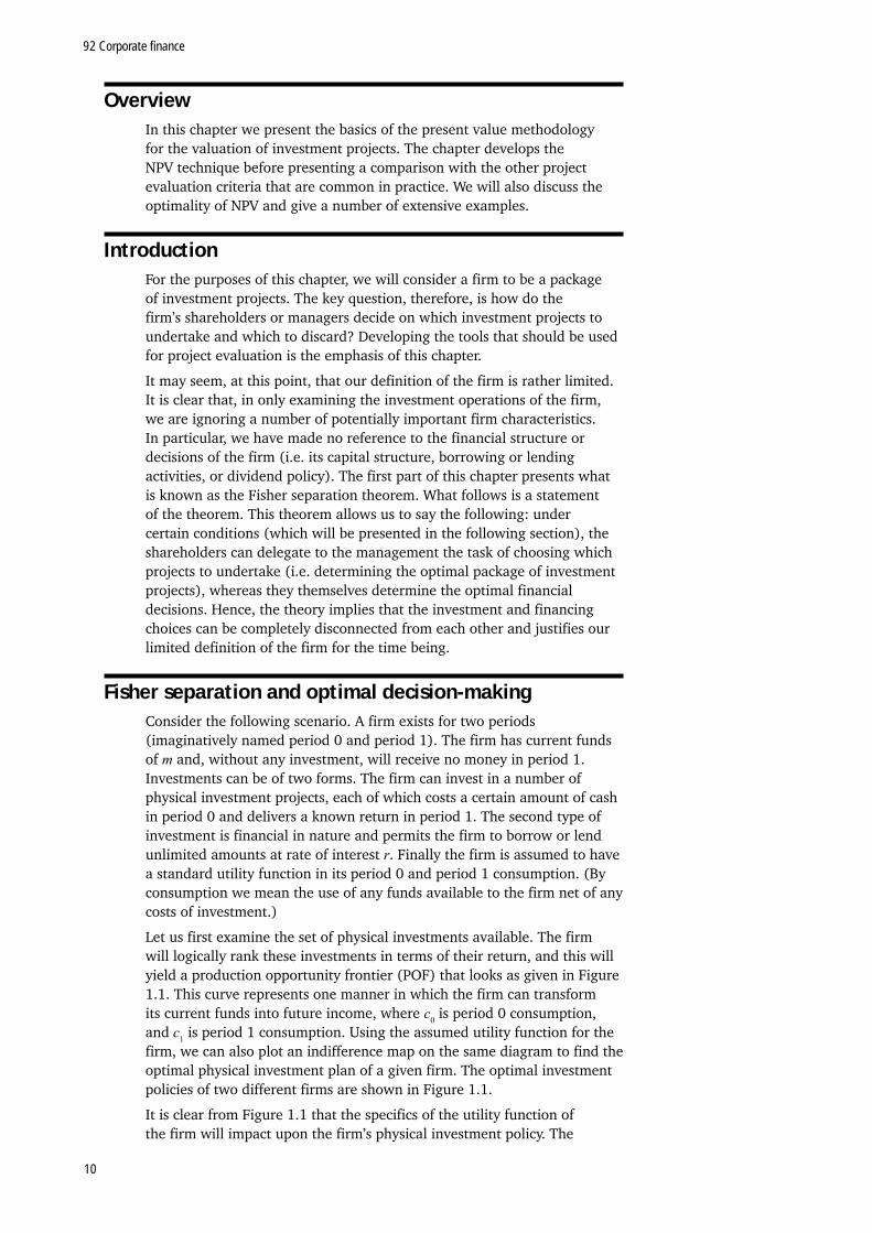
Let us first examine the set of physical investments available. The firm will logically rank these investments in terms of their return, and this will yield a production opportunity frontier (POF) that looks as given in Figure 1.1. This curve represents one manner in which the firm can transform its current funds into future income, where c0 is period 0 consumption, and c1 is period 1 consumption. Using the assumed utility function for the firm, we can also plot an indifference map on the same diagram to find the optimal physical investment plan of a given firm. The optimal investment policies of two different firms are shown in Figure 1.1.
It is clear from Figure 1.1 that the specifics of the utility function of the firm will impact upon the firm’s physical investment policy. The
Chapter 1: Present value calculations and the valuation of physical investment projects
11
implication of this is that the shareholders of a firm (i.e. those whose utility function matters in forming optimal investment policy) must dictate to the managers of the firm the point to which it invests. However, until now we have ignored the fact that the firm has an alternative method for investment (i.e. using the capital market).
Figure 1.1
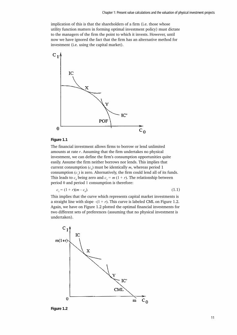
The financial investment allows firms to borrow or lend unlimited amounts at rate r. Assuming that the firm undertakes no physical investment, we can define the firm’s consumption opportunities quite easily. Assume the firm neither borrows nor lends. This implies that current consumption (c0) must be identically m, whereas period 1 consumption (c1) is zero. Alternatively, the firm could lend all of its funds. This leads to c0 being zero and c1 = m (1 + r). The relationship between period 0 and period 1 consumption is therefore:
c1 = (1 + r)(m – c0). (1.1)
This implies that the curve which represents capital market investments is a straight line with slope –(1 + r). This curve is labeled CML on Figure 1.2. Again, we have on Figure 1.2 plotted the optimal financial investments for two different sets of preferences (assuming that no physical investment is undertaken).
Figure 1.2
92 Corporate finance
12
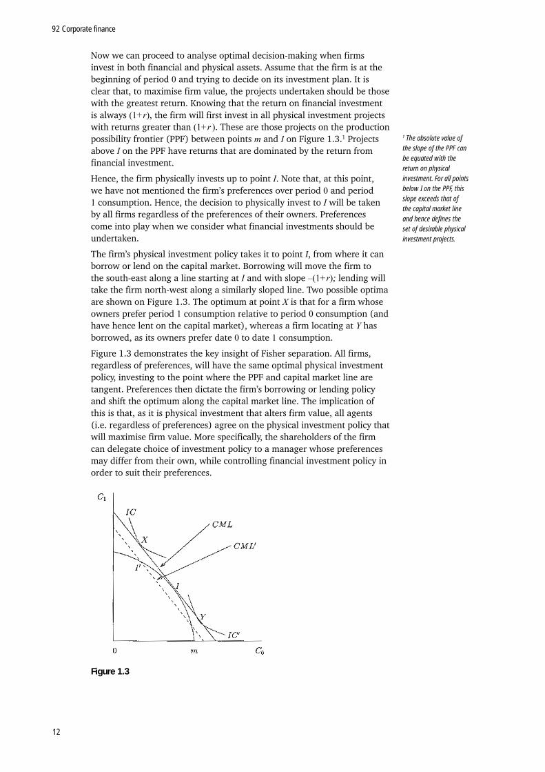
Now we can proceed to analyse optimal decision-making when firms invest in both financial and physical assets. Assume that the firm is at the beginning of period 0 and trying to decide on its investment plan. It is clear that, to maximise firm value, the projects undertaken should be those with the greatest return. Knowing that the return on financial investment is always (1+r), the firm will first invest in all physical investment projects with returns greater than (1+r ). These are those projects on the production possibility frontier (PPF) between points m and I on Figure 1.3.1 Projects above I on the PPF have returns that are dominated by the return from financial investment.
Hence, the firm physically invests up to point I. Note that, at this point, we have not mentioned the firm’s preferences over period 0 and period 1 consumption. Hence, the decision to physically invest to I will be taken by all firms regardless of the preferences of their owners. Preferences come into play when we consider what financial investments should be undertaken.
The firm’s physical investment policy takes it to point I, from where it can borrow or lend on the capital market. Borrowing will move the firm to the south-east along a line starting at I and with slope –(1+r); lending will take the firm north-west along a similarly sloped line. Two possible optima are shown on Figure 1.3. The optimum at point X is that for a firm whose owners prefer period 1 consumption relative to period 0 consumption (and have hence lent on the capital market), whereas a firm locating at Y has borrowed, as its owners prefer date 0 to date 1 consumption.
Figure 1.3 demonstrates the key insight of Fisher separation. All firms, regardless of preferences, will have the same optimal physical investment policy, investing to the point where the PPF and capital market line are tangent. Preferences then dictate the firm’s borrowing or lending policy and shift the optimum along the capital market line. The implication of this is that, as it is physical investment that alters firm value, all agents (i.e. regardless of preferences) agree on the physical investment policy that will maximise firm value. More specifically, the shareholders of the firm can delegate choice of investment policy to a manager whose preferences may differ from their own, while controlling financial investment policy in order to suit their preferences.
Figure 1.3
1 The absolute value of the slope of the PPF can be equated with the return on physical investment. For all points below I on the PPF, this slope exceeds that of the capital market line and hence defi nes the set of desirable physical investment projects.
Chapter 1: Present value calculations and the valuation of physical investment projects
13
Fisher separation and project evaluationFisher separation can also be used to justify a certain method of project appraisal. Figure 1.3 shows a suboptimal physical investment decision (I’) and the capital market line that borrowing and lending from point I’ would trace out. Clearly this capital market line always lies below that achieved through the optimal physical investment policy. Hence, one could say that optimal physical investment should maximise the horizontal intercept of the capital market line on which the firm ends up. Let us, then, assume a firm that decides to invest a dollar amount of I0. Given that the firm has date 0 income of m and no date 1 income, aside from that accruing from physical investment, the horizontal intercept of the capital market line upon which the firm has located is:
where Π(I0) is the date 1 income from the firm’s physical investment. Maximising this is equivalent to the following maximisation problem:
.
The prior objective is the NPV rule for project appraisal. It says that an optimal physical investment policy maximises the difference between investment proceeds divided by one plus the interest rate and the investment cost. Here, the term ‘optimal’ is being defined as that which leads to maximisation of shareholder utility. We will discuss the NPV rule more fully (and for cases involving more than one time period) later in this chapter.
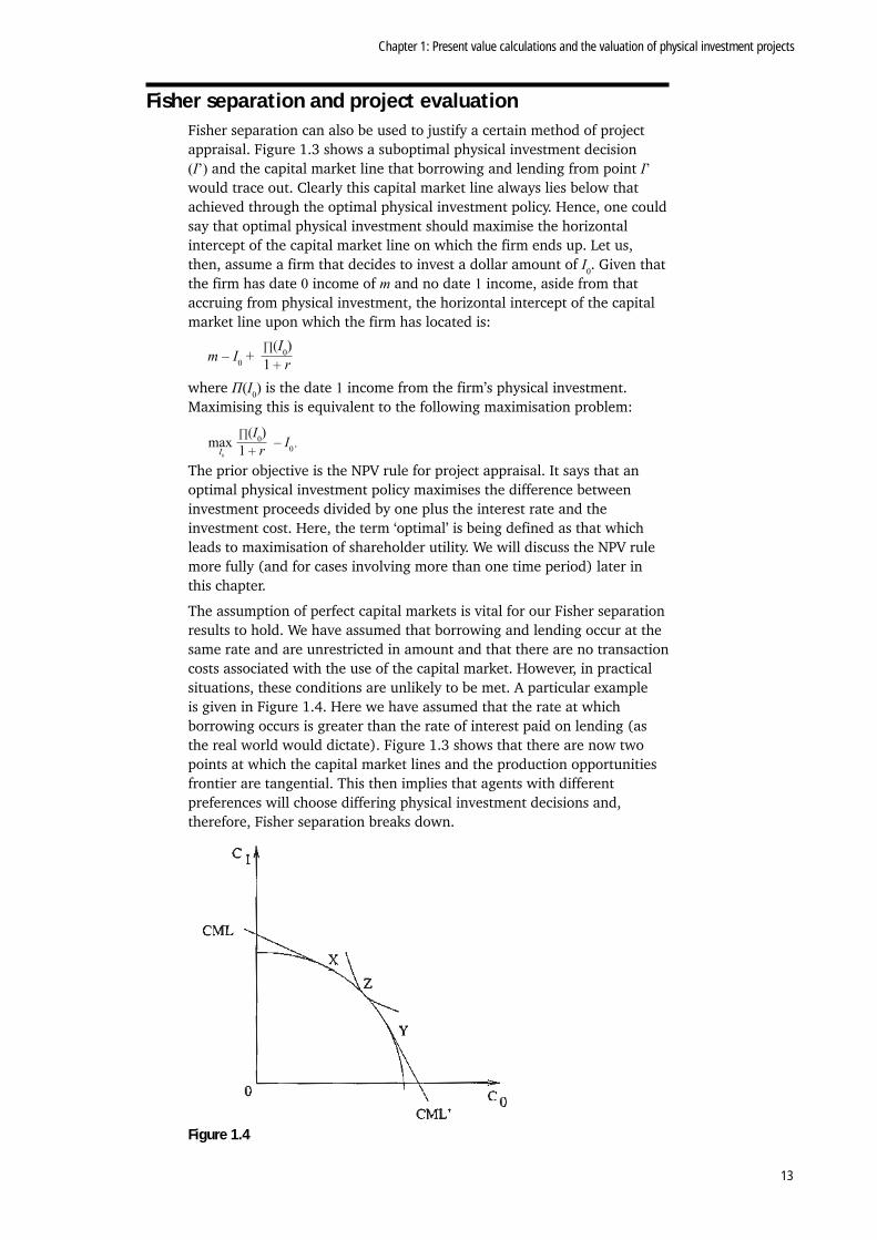
The assumption of perfect capital markets is vital for our Fisher separation results to hold. We have assumed that borrowing and lending occur at the same rate and are unrestricted in amount and that there are no transaction costs associated with the use of the capital market. However, in practical situations, these conditions are unlikely to be met. A particular example is given in Figure 1.4. Here we have assumed that the rate at which borrowing occurs is greater than the rate of interest paid on lending (as the real world would dictate). Figure 1.3 shows that there are now two points at which the capital market lines and the production opportunities frontier are tangential. This then implies that agents with different preferences will choose differing physical investment decisions and, therefore, Fisher separation breaks down.
Figure 1.4
92 Corporate finance
14
Agents with strong preferences for future consumption will physically invest to point X and then financially invest to an optimum on the capital market lending line (CML). Those with strong preferences for current consumption physically invest to point Y and borrow (along CML’). Finally, a set of agents may exist who value current and future consumption similarly, and these will optimise by locating directly on the PPF and not using the capital market at all. An example of an optimum of this type is point Z on Figure 1.4.
The time value of moneyIn the preceding section we demonstrated the Fisher separation theorem and the manner in which physical and financial investment decisions can be disconnected. The major implication of this theorem is that the set of desirable physical investment projects does not depend on the preferences of individuals. In the following sections we shall focus on the way in which individual physical investment projects should be evaluated. Our key methodology for this will be the NPV rule, mentioned in the preceding section. In the following sections we will show you how to apply the rule to situations involving more than one period and with time-varying cash flows.
To begin, let us consider a straightforward question. Is $1 received today worth the same as $1 received in one year’s time? A naïve response to this question would assert that $1 is $1 regardless of when it is received, and hence the answer to the question would be yes. A more careful consideration of the question brings the opposite response however. Let’s assume I receive $1 now. If I also assume that there is a risk-free asset in which I can invest my dollar (e.g. a bank account), then in one year’s time I will receive $(1+r), assuming I invest. Here, r is the rate of return on the safe investment. Hence $1 received today is worth $(1+r) in one year. The answer to the question is therefore no. A dollar received today is worth more than a dollar received in one year or at any time in the future.
The above argument characterises the time value of money. Funds are more valuable the earlier they are received. In the previous paragraph we illustrated this by calculating the future value of $1. We can similarly illustrate the time value of money by using present values. Assume I am to receive $1 in one year’s time and further assume that the borrowing and lending rate is r. How much is this dollar worth in today’s terms? To answer this second question, put yourself in the position of a bank. Knowing that someone is certain to receive $1 in one year, what is the maximum amount you would lend him or her now? If I, as a bank, were to lend someone money for one year, at the end of the year I would require repayment of the loan plus interest (at rate r). Hence if I loaned the individual $x, I would require a repayment of $x(1+r). This implies that the maximum amount I should be willing to lend is implicitly defined by the following equation:
$x(1+r) = $1 (1.2)
such that:
(1.3)
The value for x defined in equation 1.3 is the present value of $1 received in one year’s time. This quantity is also termed the discounted value of the $1.
Chapter 1: Present value calculations and the valuation of physical investment projects
15
You can see the present and future value concepts pictured in Figure 1.2. If you recall, Figure 1.2 just plots the CML for a given level of initial funds (m) assuming no funds are to be received in the future. The future value of this amount of money is simply the vertical intercept of the CML (i.e. m(1+r)), and obviously the present value of m(1+r) is just m.
The present and future value concepts are straightforwardly extended to cover more than one period. Assume an annual compound interest rate of r. The present value of $100 to be received in k year’s time is:
(1.4)
whereas the future value of $100 received today and evaluated k years hence is:
FVK (100) = 100(1 + r)K. (1.5)
Activity
Below, there are a few applications of the present and future value concepts. You should attempt to verify that you can replicate the calculations.
Assume a compound borrowing and lending rate of 10 per cent annually.
a. The present value of $2,000 to be received in three years time is $1,502.63.
b. The present value of $500 to be received in five years time is $310.46.
c. The future value of $6,000 evaluated four years hence is $8,784.60.
d. The future value of $250 evaluated 10 years hence is $648.44.
The net present value ruleIn the previous section we demonstrated that the value of funds depends critically on the time those funds are received. If received immediately, cash is more valuable than if it is to be received in the future.
The NPV rule was introduced in simple form in the section on Fisher separation. In its more general form, it uses the discounting techniques provided in the previous section in order to generate a method of evaluating investment projects. Consider a hypothetical physical investment project, which has an immediate cost of I. The project generates cash flows to the firm in each of the next k years, equal to Ck. In words, all that the NPV rule does is to compute the present value of all receipts or payments. This allows direct comparisons of monetary values, as all are evaluated at the same point in time. The NPV of the project is then just the sum of the present values of receipts, less the sum of the present values of the payments.
Using the notation given above and again assuming a rate of return of r, the NPV can be written as:
. (1.6)
Note that the cash flows to the project can be positive and negative, implying that the notation employed is flexible enough to embody both cash inflows and outflows after initiation.
Once we have calculated the NPV, what should we do? Clearly, if the NPV is positive, it implies that the present value of receipts exceeds the present value of payments. Hence, the project generates revenues that outweigh its costs and should therefore be accepted. If the NPV is negative the project should be rejected, and if it is zero the firm will be indifferent between accepting and rejecting the project.

92 Corporate finance
16
This gives a very straightforward method for project evaluation. Compute the NPV of the project (which is a simple calculation), and if it is greater than zero, the project is acceptable.
Example
Consider a manufacturing firm, which is contemplating the purchase of a new piece of plant. The rate of interest relevant to the firm is 10 per cent. The purchase price is £1,000. If purchased, the machine will last for three years and in each year generate extra revenue equivalent to £750. The resale value of the machine at the end of its lifetime is zero. The NPV of this project is:
NPV = 750 + 750 + 750 – 1000 = 865.14. (1.1)3 (1.1)2 (1.1)1
As the NPV of the project exceeds zero, it should be accepted.
In order to familiarise yourself with NPV calculations, attempt the following activities by calculating the NPV of each project and assessing its desirability.
Activity
Assume an interest rate of 5 per cent. Compute the NPV of each of the following projects, and state whether each project should be accepted or not.
• Project A has an immediate cost of $5,000, generates $1,000 for each of the next six years and zero thereafter.
• Project B costs £1,000 immediately, generates cash flows of £600 in year 1, £300 in year 2 and £300 in year 3.
• Project C costs ¥10,000 and generates ¥6,000 in year 1. Over the following years, the cash flows decline by ¥2,000 each year, until the cash flow reaches zero.
• Project D costs £1,500 immediately. In year 1 it generates £1,000. In year 2 there is a further cost of £2,000. In years 3, 4 and 5 the project generates revenues of £1,500 per annum.
Up to this point we have just considered single projects in isolation, assuming that our funds were enough to cover the costs involved. What happens, first of all, if the members of a set of projects are mutually exclusive?2 The answer is simple. Pick the project that has the greatest NPV. Second, what should we do if we have limited funds? It may be the case that we are faced with a pool of projects, all of which have positive NPVs, but we only have access to an amount of money that is less than the total investment cost of the entire project pool. Here we can rely on another nice feature of the NPV technique. NPVs are additive across projects (i.e. the NPV of taking on projects A and B is identical to the NPV of A plus the NPV of B). The reason for this should be obvious from the manner in which NPVs are calculated. Hence, in this scenario, we should calculate all project combinations that are feasible (i.e. the total investment in these projects can be financed with our current funds). Then calculate the NPV of each combination by summing the NPVs of its constituents, and finally choose the combination that yields the greatest total NPV.
Finally, we should devote some time to discussion of the ‘interest rate’ we have used to discount future cash flows. Until now we have just referred to r as the rate at which one can borrow or lend funds. A more precise definition of r is that r is the opportunity cost of capital. If we are considering the use of the NPV rule within the context of a firm, we have to recognise that the firm has several sources of capital, and the cost of each of these should be taken into account when evaluating the firm’s
2 By this we mean that taking on any one of the set of projects precludes us from accepting any of the others.
Chapter 1: Present value calculations and the valuation of physical investment projects
17
overall cost of capital. The firm can raise funds via equity issues and debt issues, and it is likely that the costs of these two types of funds will differ. Later on in this chapter and in those that follow, we will present techniques by which the firm can compute the overall cost of capital for its enterprise.
Other project appraisal techniquesThe NPV methodology for project appraisal is by no means the only technique used by firms to decide on their physical investment policy. It is, however, the optimal technique for corporate management to use if they wish to maximise expected shareholder wealth. This result is obvious from our Fisher separation analysis. In this section we talk about three of NPV’s competitors, the payback rule, the internal rate of return (IRR) rule, and the multiples method, which are sometimes used in practice.
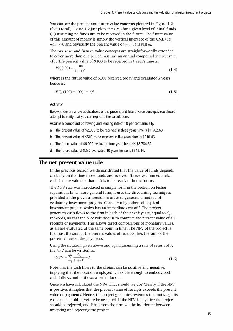
The payback rulePayback is a particularly simple criterion for deciding on the desirability of an investment project. The firm chooses a fixed payback period, for example, three years. If a project generates enough cash in the first three years of its existence to repay the initial investment outlay, then it is desirable, and if it doesn’t generate enough cash to cover the outlay, it should be rejected. Take the cash-flow stream given in the following table as an example.
Year 0 1 2 3 4
Cash flow –1,000 250 250 250 500
Table 1.1
A firm that has chosen a payback period of three years and is faced with the project shown in Table 1.1 will reject it as the cash flow in years 1 to 3 (750) doesn’t cover the initial outlay of 1,000. Note, however, that if the firm used a payback period of four years, the project would be acceptable, as the total cash flow to the project would be 1,250, which exceeds the outlay. Hence, it’s clear that the crucial choice by management is of the payback period.
We can also use the preceding example to illustrate the weaknesses of payback. First, assume that the firm has a payback period of three years. Then, as previously mentioned, the project in Table 1.1 will not be accepted. However, assume also that, instead of being 500, the project cash flow in year 4 is 500,000. Clearly, one would want to revise one’s opinion on the desirability of the project, but the payback rule still says you should reject it. Payback is flawed, as a portion of the cash-flow stream (that realised after the payback period is up) is always ignored in project evaluation.
The second weakness of payback should be obvious, given our earlier discussion of NPV. Payback ignores the time value of money. Sticking with the example in Table 1.1, assume a firm has a payback period of four years. Then the project as given should be accepted (as total cash flow of 1,250 exceeds investment outlay of 1,000). But what’s the NPV of this project? If we assume, for example, a required rate of return of 10 per cent, then the NPV can be shown to be negative. (In fact the NPV is –36.78. As a self-assessment activity, show that this is the case.) Hence application of the payback rule tells us to accept a project that would decrease expected shareholder wealth (as shown by application of the NPV rule). This flaw could be eliminated by discounting project cash flows that accrue within
92 Corporate finance
18
the payback period, giving a discounted payback rule, but such a modification still wouldn’t solve the first problem we highlighted.
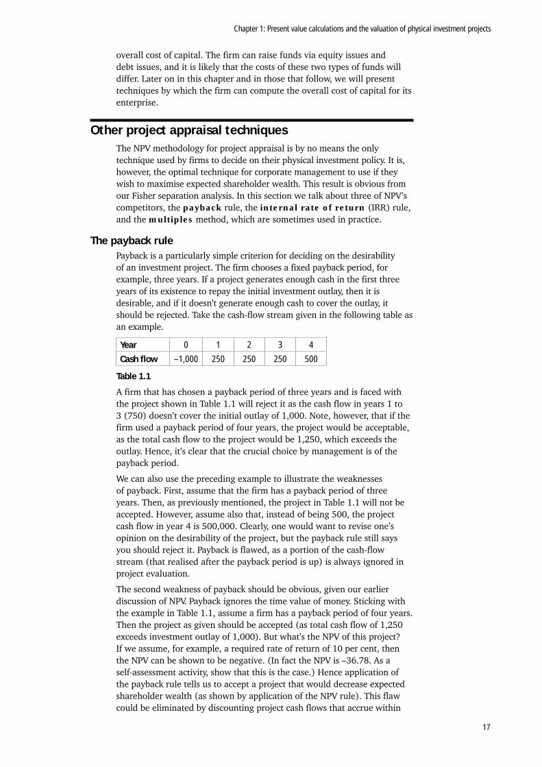
The internal rate of return ruleThe IRR rule can be viewed as a variant on the apparatus we used in the NPV formulation. The IRR of a project is the rate of return that solves the following equation:
(1.7)
where Ci is the project cash flow in year i, and I is the initial (i.e. year 0) investment outlay. Comparison of equation 1.7 with 1.6 shows that the project IRR is the discount rate that would set the project NPV to zero. Once the IRR has been calculated, the project is evaluated by comparing the IRR to a predetermined required rate of return known as a hurdle rate. If the IRR exceeds the hurdle rate, then the project is acceptable, and if the IRR is less than the hurdle rate it should be rejected. A graphical analysis of this is presented in Figure 1.5, which plots project NPV against the rate of return used in the NPV calculation. If r* is the hurdle rate used in project evaluation, then the project represented by the curve on the figure is acceptable as the IRR exceeds r*. Clearly, if r* is also the correct required rate of return, which would be used in NPV calculations, then application of the IRR and NPV rules to assessment of the project in Figure 1.5 gives identical results (as at rate r* the NPV exceeds zero).
Figure 1.5
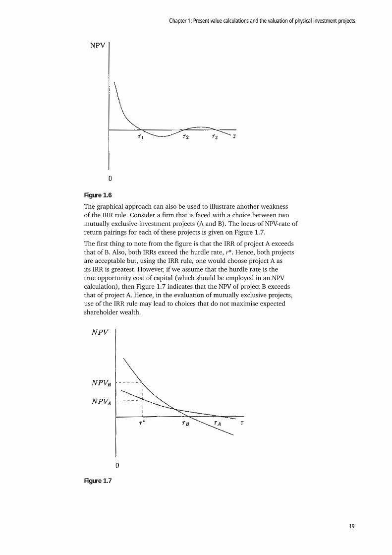
Calculation of the IRR need not be straightforward. Rearranging equation 1.7 shows us that the IRR is a solution to a kth order polynomial in r. In general, the solution must be found by some iterative process, for example, a (progressively finer) grid search method. This also points to a first weakness of the IRR approach; as the solution to a polynomial, the IRR may not be unique. Several different rates of return might satisfy equation 1.7; in this case, which one should be used as the IRR? Figure 1.6 gives a graphical example of this case.
Chapter 1: Present value calculations and the valuation of physical investment projects
19
Figure 1.6
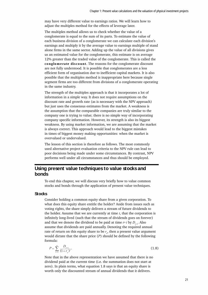
The graphical approach can also be used to illustrate another weakness of the IRR rule. Consider a firm that is faced with a choice between two mutually exclusive investment projects (A and B). The locus of NPV-rate of return pairings for each of these projects is given on Figure 1.7.
The first thing to note from the figure is that the IRR of project A exceeds that of B. Also, both IRRs exceed the hurdle rate, r*. Hence, both projects are acceptable but, using the IRR rule, one would choose project A as its IRR is greatest. However, if we assume that the hurdle rate is the true opportunity cost of capital (which should be employed in an NPV calculation), then Figure 1.7 indicates that the NPV of project B exceeds that of project A. Hence, in the evaluation of mutually exclusive projects, use of the IRR rule may lead to choices that do not maximise expected shareholder wealth.
Figure 1.7

92 Corporate finance
20
The multiples methodAn alternative to using forecasts of a firm’s or project’s cash flows to calculate value, market information can be used to estimate the value. The multiples method assesses the firm’s value based on the value of a comparable publically traded firm. For example, consider the firm’s market value to earnings ratio, this ratio tells us how much a dollar of earnings contributes to the present value according to the market’s consensus view. For publically traded firms, this ratio is available. The firm we wish to value may not have a publically available market value, however we are likely to know its earnings. If we assume that these two firms should have similar market value to earnings ratios, then we can value the firm by taking the publically available ratio and multiplying it by the firm’s earnings.
Common multiples to use are market value to earnings, market value to EBITDA, market value to cash flow, and market value to book value. Some firms, especially younger firms, have no earnings or even negative earnings. In this case it may be better to value the firm as of some future date in which the firm’s cash flows have stabilised, and then to discount to today’s value. An alternative is to use more creative multiples, for example price to patent ratio, price to subscriber ratio, or price to Ph.D. ratio. It is often better to take an average over several comparable firms to calculate the multiple. If you believe the firm being valued is better or worse than the comparable firms, you can shade the multiple down or up, as in the example below. The multiples method is not an exact science but rather a convenient way to incorporate market beliefs. It should always be used in conjunction with another method, such as NPV.
Example
Below are the equity values, debt values, and earnings (in billions) for several large US retailers. Additionally provided is earnings growth for the past 10 years.
Equity Debt E E (10 yr) %
JCP 17.48 3.81 1.10 7.8
COST 24.08 2.22 1.10 15.5
HD 82.08 12.39 6.01 21.2
WMT ? 47.44 11.88 15.7
TGT 50.14 14.14 2.58 19.2
Walmart’s (WMT’s) equity value is excluded as this is the quantity we wish to estimate. We can first calculate the market value of equity to earnings ratio for the average firm in the industry (excluding Walmart), this is: [(17.48/1.1) + (24.08/1.1) + (82.08/6.01) + (50.14/2.58)]/4 = 17.72
We now multiply this number by Walmart’s earnings to get Walmart’s equity value estimate: 17.72*11.88=210.49. Walmart’s actual equity value was $192.48 billion.
In the example above we used multiples to value equity, we sometimes wish to the value of the full business (sometimes called enterprise value), in this case we would need to use the full business value (for example, debt plus equity) in the numerator instead of just equity value.
Notice that the debt to equity ratio of Costco (COST) was 9.2% while that of Target (TGT) was 28.2%. In this example, we have ignored the effects of leverage (debt in the capital structure), however as we will see in a later chapter, leverage affects both firm value and the expected return on equity. Therefore, firms with different leverage ratios that look otherwise similar
Chapter 1: Present value calculations and the valuation of physical investment projects
21
may have very different value to earnings ratios. We will learn how to adjust the multiples method for the effects of leverage later.
The multiples method allows us to check whether the value of a conglomerate is equal to the sum of its parts. To estimate the value of each business division of a conglomerate we can calculate each division’s earnings and multiply it by the average value to earnings multiple of stand alone firms in the same sector. Adding up the value of all divisions gives us an estimated value for the conglomerate, this estimate is on average 12% greater than the traded value of the conglomerate. This is called the conglomerate discount. The reasons for the conglomerate discount are not fully understood. It is possible that conglomerates are a less efficient form of organisation due to inefficient capital markets. It is also possible that the multiples method is inappropriate here because single segment firms are too different from divisions of a conglomerate operating in the same industry.
The strength of the multiples approach is that it incorporates a lot of information in a simple way. It does not require assumptions on the discount rate and growth rate (as is necessary with the NPV approach) but just uses the consensus estimates from the market. A weakness is the assumption that the comparable companies are truly similar to the company one is trying to value; there is no simple way of incorporating company specific information. However, its strength is also its biggest weakness. By using market information, we are assuming that the market is always correct. This approach would lead to the biggest mistakes in times of biggest money making opportunities: when the market is overvalued or undervalued.
The lesson of this section is therefore as follows. The most commonly used alternative project evaluation criteria to the NPV rule can lead to poor decisions being made under some circumstances. By contrast, NPV performs well under all circumstances and thus should be employed.
Using present value techniques to value stocks and bonds
To end this chapter, we will discuss very briefly how to value common stocks and bonds through the application of present value techniques.
StocksConsider holding a common equity share from a given corporation. To what does this equity share entitle the holder? Aside from issues such as voting rights, the share simply delivers a stream of future dividends to the holder. Assume that we are currently at time t, that the corporation is infinitely long-lived (such that the stream of dividends goes on forever) and that we denote the dividend to be paid at time t+i by Dt+i. Also assume that dividends are paid annually. Denoting the required annual rate of return on this equity share to be re, then a present value argument would dictate that the share price (P) should be defined by the following formula:
. (1.8)
Note that in the above representation we have assumed that there is no dividend paid at the current time (i.e. the summation does not start at zero). In plain terms, what equation 1.8 says is that an equity share is worth only the discounted stream of annual dividends that it delivers.
92 Corporate finance
22
A simplification of the preceding formula is available when we assume that the dividend paid grows at constant percentage rate g per annum. Then, assuming that a dividend of D0 has just been paid, the future stream of dividends will be D0(1+g), D0(1+g)2, D0(1+g)3 and so on. This type of cash-flow stream is known as a perpetuity with growth, and its present value can be calculated very simply.3 In this setting the price of the equity share is:
0 . (1.9)
This is the Gordon growth model of equity valuation. As is obvious from the preceding discussion, it is only valid if you can assert that dividends grow at a constant rate.
Note also that if you have the share price, dividend just paid and an estimate of dividend growth, you can rearrange equation 1.9 to give the required rate of return on the stock – that is:
. (1.10)
The first term in 1.10 is the expected dividend yield on the stock, and the second is expected dividend growth. Hence, with empirical estimates of the previous two quantities, we can easily calculate the required rate of return on any equity share.
Activity
Attempt the following questions:
1. An investor is considering buying a certain equity share. The stock has just paid a dividend of £0.50, and both the investor and the market expect the future dividend to be precisely at this level forever. The required rate of return on similar equities is 8 per cent. What price should the investor be prepared to pay for a single equity share?
2. A stock has just paid a dividend of $0.25. Dividends are expected to grow at a constant annual rate of 5 per cent. The required rate of return on the share is 10 per cent. Calculate the price of the stock.
3. A single share of XYZ Corporation is priced at $25. Dividends are expected to grow at a rate of 8 per cent, and the dividend just paid was $0.50. What is the required rate of return on the stock?
BondsIn principle, bonds are just as easy to value.
• A discount or zero coupon bond is an instrument that promises to pay the bearer a given sum (known as the principal) at the end of the instrument’s lifetime. For example, a simple five-year discount bond might pay the bearer $1,000 after five years have elapsed.
• Slightly more complex instruments are coupon bonds. These not only repay the principal at the end of the term but in the interim entitle the bearer to coupon payments that are a specified percentage of the principal. Assuming annual coupon payments, a three-year bond with principal of £100 and coupon rate of 8 per cent will give annual payments of £8, £8 and £108 in years 1, 2 and 3.
In more general terms, assuming the coupon rate is c, the principal is P and the required annual rate of return on this type of bond is rb, the price of the bond can be written as:4
. (1.11)
3 See Appendix 1.
4 In our notation a coupon rate of 12 per cent, for example, implies that c = 0.12; the discount rate used here, rb , is called the yield to maturity of the bond.

Chapter 1: Present value calculations and the valuation of physical investment projects
23
Note that it is straightforward to value discount bonds in this framework by setting c to zero.
Activity
Using the previous formula, value a seven-year bond with principal $1,000, annual coupon rate of 5 per cent and required annual rate of return of 12 per cent. (Hint: the use of a set of annuity tables might help.)
A reminder of your learning outcomesHaving completed this chapter, and the Essential reading and activities, you should be able to:
• analyse optimal physical and financial investment in a perfect capital markets setting and derive the Fisher separation result
• justify the use of the NPV rules via Fisher separation
• compute present and future values of cash-flow streams and appraise projects using the NPV rule
• evaluate the NPV rule in relation to other commonly used evaluation criteria
• value stocks and bonds via NPV.
Key termscapital market line (CML)
consumption
Fisher separation theorem
Gordon growth model
indifference curve
internal rate of return (IRR) rule
investment policy
net present value (NPV) rule
payback rule
production opportunity frontier (POF)
production possibility frontier (PPF)
time value of money
utility function
Sample examination questions1. The Toyundai Motor Company has the opportunity to invest in new
production line equipment, which would have a working lifetime of 10 years. The new equipment would generate the following increases in Toyundai’s net cash flows.
In the first year of usage the new plant would decrease costs by $200,000. For the following six years the cost saving would fall at a rate of 5 per cent per annum. In the remaining years of the equipment’s lifetime, the annual cost saving would be $140,000. Assuming that the cost of the equipment is $1,000,000 and that Toyundai’s cost of capital is 10 per cent, calculate the NPV of the project. Should Toyundai take on the investment? (15%)

92 Corporate finance
24
2. Describe two methods of project evaluation other than NPV. Discuss the weaknesses of these methods when compared to NPV. (10%)
3. The CEO and other top executives of a firm with no nearby commercial airports make approximately 300 flights per year with an average cost per flight of $5,000. The firm is considering buying a Gulfstream jet for $15 million. The jet will reduce the cost of travel to $300,000 (including fuel, maintenance, and other jet-related expenses).
The firm expects to be able to resell the jet in five years for $12.5 million. The firm pays a 25% corporate tax on its profits and can offset its corporate liabilities by using straight line depreciation on its fixed assets. The opportunity cost of capital is 4%.
a. Should the firm buy this jet if it has sufficient taxable profits in order to take advantage of all tax shields?
b. Should the firm buy this jet if it does not have sufficient taxable profits in order to take advantage of new tax shields?
c. Suppose the firm could lease an airplane for the first year, with an option to extend the lease. Within that year they would find out whether the local government has decided to build an airport nearby which would reduce travel costs. How would this change your calculations?
4. Suppose that you have a £10,000 student loan with a 5 per cent interest rate. You also have £1,000 in your zero interest checking account which you do not plan to use in the foreseeable future. You are considering three strategies: (i) payoff as much of the loan as possible, (ii) invest the money in a local bank at 3.5 per cent interest, (iii) invest in the stock market. The expected return on the stock market is 6 per cent for the foreseeable future. Your personal discount rate is 4 per cent for risk-free investments. For simplicity assume all investments are perpetuities.
a. What is the NPV of strategy (i)?
b. What is the NPV of strategy (ii)?
c. What is the NPV of strategy (iii) if you are risk neutral?
d. What is the NPV of strategy (iv) if your subjective market risk premium is 3 per cent?

Chapter 2: Risk and return: mean–variance analysis and the CAPM
25
Chapter 2: Risk and return: mean–variance analysis and the CAPM
Aim of the chapterThe aim of this chapter is to derive the capital asset pricing model (CAPM) enabling us to price financial assets. In order to do so, we introduce the mean–variance analysis setting, in which investors care solely about financial assets’ expected returns and variances of returns, as well as the statistical tools enabling us to calculate portfolios’ expected returns and variances of returns.
Learning outcomesAt the end of this chapter, and having completed the Essential reading and activities, you should be able to:
• discuss concepts such as a portfolio’s expected return and variance as well as the covariance and correlation between portfolios’ returns
• calculate portfolio expected return and variance from the expected returns and return variances of constituent assets with confidence
• describe the effects of diversification on portfolio characteristics
• derive the CAPM using mean–variance analysis
• describe some theoretical and practical limitations of the CAPM.
Essential readingHillier, D., M. Grinblatt and S. Titman Financial Markets and Corporate Strategy.
(Boston, Mass.; London: McGraw-Hill, 2008) Chapters 4 (The Mathematics and Statistics of Portfolios) and 5 (Mean-Variance Analysis and the CAPM).
Further readingBrealey, R., S. Myers and F. Allen Principles of Corporate Finance. (Boston,
Mass.; London: McGraw-Hill, 2008) Chapters 8 (Introduction to Risk, Return, and the Opportunity Cost of Capital) and 9 (Risk and Return).
Copeland, T. and J. Weston Financial Theory and Corporate Policy. (Reading, Mass.; Wokingham: Addison-Wesley, 2005) Chapters 5 and 6.
Roll, R. ‘A critique of the asset pricing theory’s texts. Part 1: on past and potential testability of the theory’, Journal of Financial Economics 4(2) 1977, pp.129–76.
IntroductionIn Chapter 1 we examined the use of present value techniques in the evaluation of physical investment projects and in the valuation of primitive financial assets (i.e. stocks and bonds). A key input into NPV calculations is the rate of return used in the construction of the discount factor but, thus far, we have said little regarding where this rate of return comes from. Our objective in this chapter is to demonstrate how the risk of a given security or project impacts on the rate of return required from it and hence affects the value assigned to that asset in equilibrium.
92 Corporate finance
26
We begin by introducing the basic statistical tools that will be needed in our analysis, these being expected values, variances and covariances. This leads to an analysis of the statistical characteristics of portfolios of financial assets and ultimately to a presentation of the standard mean–variance optimisation problem. The key result of mean–variance analysis is known as two-fund separation, and this result underlies the CAPM, which we will present next.
Statistical characteristics of portfoliosA portfolio is a collection of different assets held by a given investor. For example, an American investor may hold 100 Microsoft shares and 650 shares of Bethlehem Steel and therefore holds a portfolio comprising two assets. The objective of this section is to arrive at the statistical characteristics of the return on the entire portfolio, given the statistical features of each of the constituent assets. The key statistical measures used are expected returns and return variances or standard deviations. The expected return on a given asset can be thought of as the reward gained from holding it, whereas the return variance is a measure of total asset risk.
Let us define notation. First, we should clarify the way in which we are thinking about asset returns. The return on an asset is assumed to be a random variable with known distributional characteristics. Each individual asset is assumed to have an expected return of E(rj) and return variance σ2
j. Assets i and j are assumed to have covariance σij . Similarly, we denote the expected return of the portfolio held as E(Rp) and its variance by σ2
P. Finally, we assume that an investor can pick from N different stocks when forming their portfolio.
Returning to the example of the American investor given above, assume that the market price of Microsoft shares is 130 and that of Bethlehem Steel is 10.1 Hence, given the numbers of each share held, the total value of this investor’s portfolio is $195. We further assume that the expected returns on Microsoft and Bethlehem Steel are 10 per cent and 16 per cent respectively, whereas their variances are 0.25 and 0.49.
We are now in a position to define the share of the entire portfolio value that is contributed by each individual stockholding. These are referred to as portfolio weights. The portfolio weight of Bethlehem Steel, for example, is simply the value of the Bethlehem Steel holding divided by $195 (i.e. 1/3 or approximately 33.3 per cent). Hence our US investor allocates 1/3 of every dollar invested to Bethlehem Steel stock.
Activity
Calculate the portfolio weight for Microsoft, using the method presented above.
From the calculations undertaken it is clear that the sum of portfolio weights must be unity. Each portfolio weight represents the share of total portfolio value contributed by a given asset. Obviously, aggregating these shares across all assets held will give a result of unity. Hence, extending the notation presented above, we denote the portfolio weight on asset i by ai, and the preceding argument implies that α1= 1.
1 These prices are in US cents.
Chapter 2: Risk and return: mean–variance analysis and the CAPM
27
Our American investor now knows the statistical characteristics of the return on each of the assets held, plus how to calculate the portfolio weight on each of the assets. What they would really like to know now is how to construct the return characteristics for the entire portfolio (i.e. they are concerned about the risk and reward associated with their entire investment). In order to do this we will need to introduce some basic properties of expectations, variances and covariances.
Expectations, variances and covariancesConsider two random variables, x and y. The expected values and variances of these variables are E(x), E(y), σ2
x and σ2y. The covariance
between the random variables is σxy.
Form an arbitrary linear combination of these two random variables and denote it P (i.e. P = ax + by, where a and b are constants). We wish to know the expected return and variance of the new random variable P. These are calculated as follows:
E(P) = aE(x) + bE(y) (2.1)
σ2P = a2σ2
x + b2σ2y + 2abσxy. (2.2)
The preceding results are readily extended to the case where more than two random variables are linearly combined. Consider N random variables denoted xi, where i runs from 1 to N. Denote their expected values and variances as E(xi) and σ2
i. The covariance between xi and xj is σij. Again we form a linear combination of the random variables, denoted again by P, using an arbitrary set of constants denoted ai. The expected value and variance of the random variable P are given by:
(2.3)
. (2.4)
Given that the returns on individual assets are assumed to be random variables with known distributional characteristics, the statistical results given above allow us to calculate portfolio returns and variances very simply.
In addition to the data on Microsoft and Bethlehem Steel provided earlier, we also need to know the covariance between Microsoft and Bethlehem Steel returns in order to determine the statistical characteristics of portfolios of these two assets. However, rather than using covariances, we shall work throughout the rest of this analysis with correlation coefficients. The relationship between correlations and covariances is given below.
Covariances and correlationsAssume two random variables, x and y, with variances denoted by σ2
x and σ2
y. The covariance between the random variables is σxy. The correlation coefficient is defined as follows:
, (2.5)
that is, the correlation between the two random variables is simply the covariance, divided by the product of the respective standard deviations. Clearly, knowledge of the correlation and the variances of the two random variables allows one to retrieve the covariance between the two random variables.
If we again define a linear combination of the two random variables, P, using arbitrary constants a and b, the expression for the variance of the
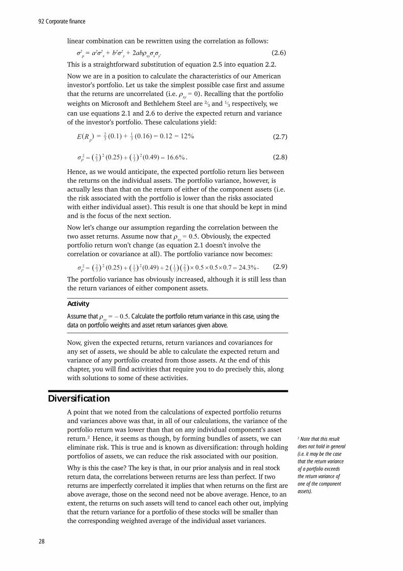
92 Corporate finance
28
linear combination can be rewritten using the correlation as follows:
σ2p = a2σ2
x + b2σ2y + 2abxyσxσy. (2.6)
This is a straightforward substitution of equation 2.5 into equation 2.2.
Now we are in a position to calculate the characteristics of our American investor’s portfolio. Let us take the simplest possible case first and assume that the returns are uncorrelated (i.e. xy = 0). Recalling that the portfolioweights on Microsoft and Bethlehem Steel are 2/
3 and 1/3 respectively, we
can use equations 2.1 and 2.6 to derive the expected return and variance of the investor’s portfolio. These calculations yield:
(2.7)
. (2.8)
Hence, as we would anticipate, the expected portfolio return lies between the returns on the individual assets. The portfolio variance, however, is actually less than that on the return of either of the component assets (i.e. the risk associated with the portfolio is lower than the risks associated with either individual asset). This result is one that should be kept in mind and is the focus of the next section.
Now let’s change our assumption regarding the correlation between the two asset returns. Assume now that xy = 0.5. Obviously, the expected portfolio return won’t change (as equation 2.1 doesn’t involve the correlation or covariance at all). The portfolio variance now becomes:
. (2.9)
The portfolio variance has obviously increased, although it is still less than the return variances of either component assets.
Activity
Assume that xy = – 0.5. Calculate the portfolio return variance in this case, using the data on portfolio weights and asset return variances given above.
Now, given the expected returns, return variances and covariances for any set of assets, we should be able to calculate the expected return and variance of any portfolio created from those assets. At the end of this chapter, you will find activities that require you to do precisely this, along with solutions to some of these activities.
DiversificationA point that we noted from the calculations of expected portfolio returns and variances above was that, in all of our calculations, the variance of the portfolio return was lower than that on any individual component’s asset return.2 Hence, it seems as though, by forming bundles of assets, we can eliminate risk. This is true and is known as diversification: through holding portfolios of assets, we can reduce the risk associated with our position.
Why is this the case? The key is that, in our prior analysis and in real stock return data, the correlations between returns are less than perfect. If two returns are imperfectly correlated it implies that when returns on the first are above average, those on the second need not be above average. Hence, to an extent, the returns on such assets will tend to cancel each other out, implying that the return variance for a portfolio of these stocks will be smaller than the corresponding weighted average of the individual asset variances.
2 Note that this result does not hold in general (i.e. it may be the case that the return variance of a portfolio exceeds the return variance of one of the component assets).

Chapter 2: Risk and return: mean–variance analysis and the CAPM
29
To illustrate this point in a general setting, consider the following scenario. An investor holds a portfolio consisting of N stocks, with each stock having the same portfolio weight (i.e. each stock has portfolio weight N–1). Denote the return variances for the individual assets by σ2
i where i = 1 to N, and the covariance between returns on assets i and j by σij. Using equation 2.4, the variance of the investor’s portfolio return can be written as:
. (2.10)
Examining the second term of equation 2.10, the existence of N component assets implies that the summation for all i not equal to j involves N(N – 1) terms. Obviously the summation in the first term of equation 2.10 involves N terms. Hence, defining the average variance of the N assets as σ2 and average covariance across all assets as C, equation 2.10 can be rewritten as:
. (2.11)
Equation 2.11 obviously simplifies to the following:
. (2.12)
Now we ask the following question. How does the portfolio variance change as the number of assets combined in the portfolio increases towards infinity (i.e. N ). It is clear from equation 2.12 that, as the number of assets held increases, the first term will shrink towards zero. Also, as N increases the second term in equation 2.12 tends towards C. Together, these observations imply the following:
1. The portfolio variance falls as the number of assets held increases.
2. The limiting portfolio return variance is simply the average covariance between asset returns: this average covariance can be thought of as the risk of the market as a whole, with the influence of individual asset return variances disappearing in the limit.
The moral of the preceding statistical story is clear. Holding portfolios consisting of greater and greater numbers of assets allows an investor to reduce the risk that they bear. This is illustrated diagrammatically in Figure 2.1.
Figure 2.1
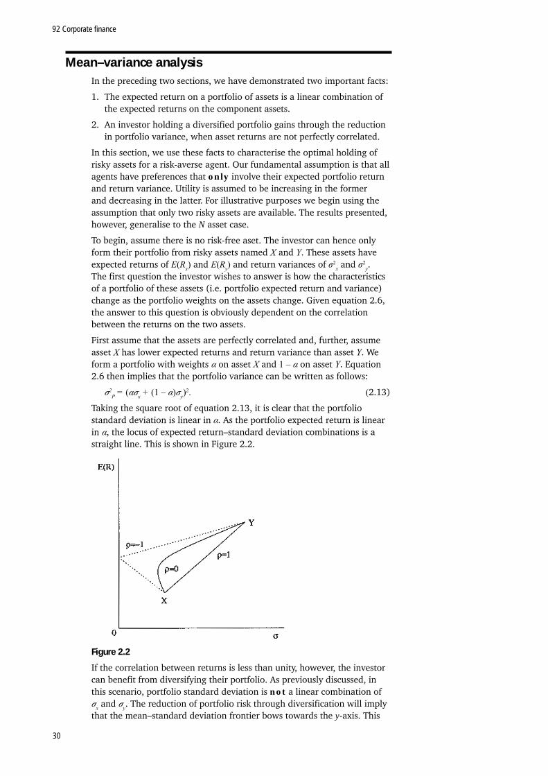
92 Corporate finance
30
Mean–variance analysisIn the preceding two sections, we have demonstrated two important facts:
1. The expected return on a portfolio of assets is a linear combination of the expected returns on the component assets.
2. An investor holding a diversified portfolio gains through the reduction in portfolio variance, when asset returns are not perfectly correlated.
In this section, we use these facts to characterise the optimal holding of risky assets for a risk-averse agent. Our fundamental assumption is that all agents have preferences that only involve their expected portfolio return and return variance. Utility is assumed to be increasing in the former and decreasing in the latter. For illustrative purposes we begin using the assumption that only two risky assets are available. The results presented, however, generalise to the N asset case.
To begin, assume there is no risk-free aset. The investor can hence only form their portfolio from risky assets named X and Y. These assets have expected returns of E(Rx) and E(Ry) and return variances of σ2
x and σ2y.
The first question the investor wishes to answer is how the characteristics of a portfolio of these assets (i.e. portfolio expected return and variance) change as the portfolio weights on the assets change. Given equation 2.6, the answer to this question is obviously dependent on the correlation between the returns on the two assets.
First assume that the assets are perfectly correlated and, further, assume asset X has lower expected returns and return variance than asset Y. We form a portfolio with weights α on asset X and 1 – α on asset Y. Equation 2.6 then implies that the portfolio variance can be written as follows:
σ2P = (ασx + (1 – α)σy)
2. (2.13)
Taking the square root of equation 2.13, it is clear that the portfolio standard deviation is linear in α. As the portfolio expected return is linear in α, the locus of expected return–standard deviation combinations is a straight line. This is shown in Figure 2.2.
Figure 2.2
If the correlation between returns is less than unity, however, the investor can benefit from diversifying their portfolio. As previously discussed, in this scenario, portfolio standard deviation is not a linear combination of σx and σy. The reduction of portfolio risk through diversification will imply that the mean–standard deviation frontier bows towards the y-axis. This
Chapter 2: Risk and return: mean–variance analysis and the CAPM
31
is also shown on Figure 2.2. The final curve on Figure 2.2 represents the case where returns are perfectly negatively correlated. In this situation, a portfolio can be constructed, which has zero standard deviation.
Activities
1. Assuming asset returns are perfectly negatively correlated, use equation 2.6 to find the portfolio weights that give a portfolio with zero standard deviation. (Hint: write down 2.6 with the correlation set to minus one and a = and b = 1 – . Then minimise portfolio variance with respect to .)
2. Assume that the returns on Microsoft and Bethlehem Steel have a correlation of 0.5. Using the data provided earlier in the chapter, construct the mean–variance frontier for portfolios of these two assets. Start with a portfolio consisting only of Microsoft stock and then increase the portfolio weight on Bethlehem Steel by 0.1 repeatedly, until the portfolio consists of Bethlehem Steel stock only.
From here on we will assume that return correlation is between plus and minus one. The expected return–standard deviation locus for this case is redrawn in Figure 2.3. In the absence of a risk-free asset, this locus is named the mean–variance frontier. As our investor’s preferences are increasing in expected return and decreasing in standard deviation, it is clear that their optimal portfolio will always lie on the frontier and to the right of the point labelled V. This point represents the minimum-variance portfolio. They will always choose a frontier portfolio at or to the right of V, as these portfolios maximise expected return for a given portfolio standard deviation. In the absence of a risk-free asset, this set of portfolios is called the efficient set.
Figure 2.3
We can now, given a set of preferences for the investor, find their optimal portfolio. The condition characterising the optimum is that an investor’s indifference curve must be tangent to the mean–variance frontier.3 Two such optima are identified on Figure 2.3 at R and S. The investor locating at equilibrium point R is relatively risk-averse (i.e. their indifference curves are quite steep), whereas the equilibrium at S is that for a less risk-averse individual (with correspondingly flatter indifference curves). Figure 2.3 also shows suboptimal indifference curves for each set of preferences.
Hence, as Figure 2.3 demonstrates, in a world of two risky assets and no risk-free asset, the optimal portfolio of risky assets held by an investor depends on their preferences towards risk and return. The same is true
3 In technical terms, the optimum is characterised by the marginal rate of substitution being equal to the marginal rate of transformation (i.e. the slope of the indifference curve equals the slope of the frontier).
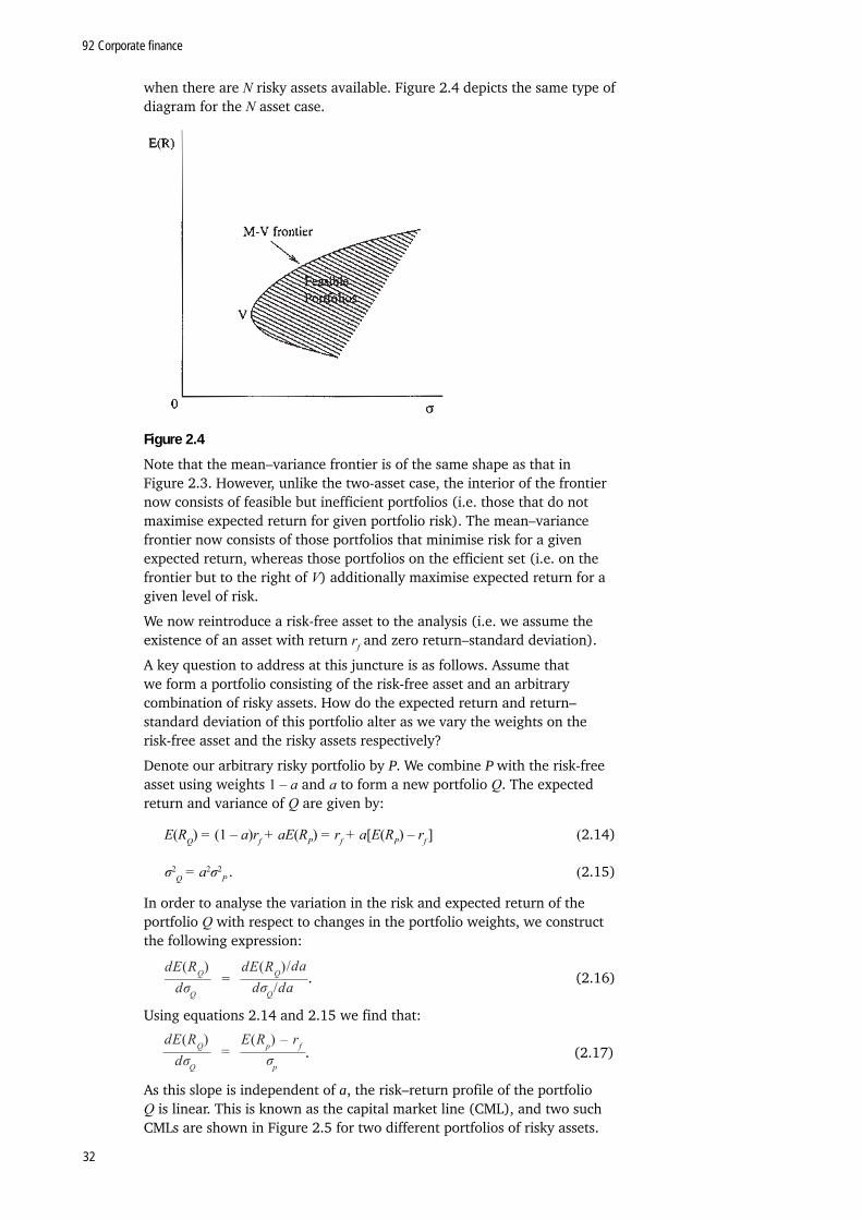
92 Corporate finance
32
when there are N risky assets available. Figure 2.4 depicts the same type of diagram for the N asset case.
Figure 2.4
Note that the mean–variance frontier is of the same shape as that in Figure 2.3. However, unlike the two-asset case, the interior of the frontier now consists of feasible but inefficient portfolios (i.e. those that do not maximise expected return for given portfolio risk). The mean–variance frontier now consists of those portfolios that minimise risk for a given expected return, whereas those portfolios on the efficient set (i.e. on the frontier but to the right of V) additionally maximise expected return for a given level of risk.
We now reintroduce a risk-free asset to the analysis (i.e. we assume the existence of an asset with return rf and zero return–standard deviation).
A key question to address at this juncture is as follows. Assume that we form a portfolio consisting of the risk-free asset and an arbitrary combination of risky assets. How do the expected return and return–standard deviation of this portfolio alter as we vary the weights on the risk-free asset and the risky assets respectively?
Denote our arbitrary risky portfolio by P. We combine P with the risk-free asset using weights 1 – a and a to form a new portfolio Q. The expected return and variance of Q are given by:
E(RQ) = (1 – a)rf + aE(RP) = rf + a[E(RP) – rf ] (2.14)
σ2Q = a2σ2
P . (2.15)
In order to analyse the variation in the risk and expected return of the portfolio Q with respect to changes in the portfolio weights, we construct the following expression:
. (2.16)
Using equations 2.14 and 2.15 we find that:
. (2.17)
As this slope is independent of a, the risk–return profile of the portfolio Q is linear. This is known as the capital market line (CML), and two such CMLs are shown in Figure 2.5 for two different portfolios of risky assets.

Chapter 2: Risk and return: mean–variance analysis and the CAPM
33
Figure 2.5
We now have all the components required to describe the optimal portfolio choice of an investor faced with N risky assets and a risk-free investment. Figure 2.6 replots the feasible set of risky asset portfolios. The key question to answer is, what portfolio of risky assets should an investor hold? Using the analysis from Figure 2.5, it is clear that the optimal choice of risky asset portfolio is at K. Combining K with the risk-free asset places an investor on a capital market line (labelled rf KZ), which dominates in utility terms the CML generated by the choice of any other feasible portfolio of risky assets.4 The optimal portfolio choice and a suboptimal CML (labelled CML2) are shown on Figure 2.6 along with the indifference curves of two investors.
Figure 2.6
Recall that we previously defined the efficient set as the group of portfolios that both minimised risk for a given level of expected return and maximised expected return for a given level of risk. With the introduction of the risk-free asset, the efficient set is exactly the optimal CML.
The key result that is depicted in Figure 2.6 is known as two-fund separation. Any risk-averse investor (regardless of their degree of risk-aversion) can form their optimal portfolio by combining two mutual funds. The first of these is the tangency portfolio of risky assets, labelled K, and the second is the risk-free asset. All that the degree of risk-aversion dictates is the portfolio weights placed on each of the two funds. The investor with the
4 That is, choosing portfolio K places an investor on a CML with greater expected returns at each level of return variance than does any other.
92 Corporate finance
34
optimum depicted at X on Figure 2.6, for example, is relatively risk-averse and has placed positive portfolio weights on both the risk-free asset and K. An investor locating at Y, however, is less risk-averse and has sold the risk-free asset short in order to invest more in K.5
Two-fund separation is the result that underlies the CAPM, which is developed in the next section.
The capital asset pricing modelTo begin our derivation of the CAPM, we present the assumptions that underlie the analysis. These assumptions formalise those implicit in the preceding section.
• Investors maximise utility defined over expected return and return variance.
• Unlimited amounts may be borrowed or loaned at the risk-free rate.
• Investors have homogenous expectations regarding future asset returns.
• Asset markets are perfect and frictionless (e.g. no taxes on sales or purchases, no transaction costs and no short sales restrictions).
We next need to extend slightly our analysis of the previous section in order to derive the familiar form of the CAPM.
A mathematical characterisation of mean–variance optimisationConsider Figure 2.6, which graphically identifies the optimal portfolio of risky assets (K), held by an arbitrary risk-averse investor. The key condition for optimality is that the capital market line and the mean–variance frontier are tangent. The following equations give a mathematical description of this optimality condition.
From equation 2.17, we know that the slope of the capital market line at the optimum is:
(2.18)
We also need the slope of the mean–variance frontier at the point of tangency. To derive this, consider a position (called I) with portfolio weight a in an arbitrary portfolio of risky assets (called j) and (1 – a) in the optimal portfolio K. The expected return and standard deviation of this position are:
E(RI) = aE(Rj) + (1 – a)E(RK) (2.19)
σ1 = [a2σ2j + (1 – a)2σ2
K + 2a(1 – a)σjK]0.5. (2.20)
Using the same method as shown in equation 2.16 to derive the risk–return trade-off at the point represented by portfolio I, we get:
. (2.21)
(2.22)
The slope of the mean–variance frontier at K will be the ratio of 2.21 to 2.22 in the limit as a 0. Note that equation 2.21 does not depend on a. Taking the limit of equation 2.22 as a 0 we get:
. (2.23)
5 A short sale is the sale of an asset that one does not actually own. One borrows the asset in order to complete the transactions and immediately receives the sale price. Subsequently, one uses the proceeds from the sale to repurchase a unit of the asset, and deliver it to the creditor. If the price of the asset has dropped in the interim, one makes a cash profi t.
Chapter 2: Risk and return: mean–variance analysis and the CAPM
35
The slope of the mean–variance frontier at K is the ratio of 2.21 to 2.23, that is,
. (2.24)
The optimum in Figure 2.6 equates the slope of the mean–variance frontier at K with the slope of the CML. Hence, equating 2.18 and 2.24 and rearranging the resulting expression, we arrive at:
(2.25)
Defining βj = σjK / σ2K, equation 2.26 can be rewritten as:
E(Rj) = rj + βj[E(RK) – rf ]. (2.26)
Equation 2.26 is the standard β-representation of the mean–variance optimisation problem. The equation translates as follows: the expected return on a given asset (or portfolio of assets) is equal to the risk-free rate plus a risk premium multiplied by the asset’s β.6 Assets that have large values of β will have large expected returns, whereas those with smaller values of β will have low expected returns with β defined as the ratio of the covariance of an asset’s returns with those on the market to the variance of the market return.
Equilibrium and the CAPMEquation 2.26 is simply derived from mean–variance analysis, and as yet we have said nothing regarding equilibrium in asset markets. Capital market equilibrium requires that the demand for risky securities be identical to their supply. The supply of risky assets is summarised in the market portfolio, which is defined below.
DefinitionThe market portfolio is the portfolio comprising all assets, where the weights used in the construction of the portfolio are calculated as the market capitalisation of each asset divided by the sum of market capitalisations across all assets.
Two-fund separation gives us the fundamental result that all investors hold efficient portfolios and, further, that all investors hold risky securities in the same proportions (i.e. those proportions dictated by the tangency portfolio (K)).7 For demand to be equal to supply in capital markets, it must be the case that the market portfolio is constructed with identical portfolio weights. The implication of this is simple: the market portfolio and the tangency portfolio are identical. This allows us to express the CAPM in the following form.
The capital asset pricing modelUnder the prior assumptions, the following relationship holds for all expected portfolio returns:
E(Rj ) = Rf + βj [E(rM ) – rf ], (2.27)
where E(RM ) is the expected return on the market portfolio, and βj is the covariance of the returns on asset j with those on the market divided by the variance of the market return.
Equation 2.27 gives the equilibrium relationship between risk and return under the CAPM assumptions. In the CAPM framework, the relevant
6 The risk premium is defi ned as the excess of the expected return on the tangency portfolio over the risk-free rate.
7 All investors perceive the same effi cient set and tangency portfolio due to our assumption that they have homogeneous expectations regarding asset returns.
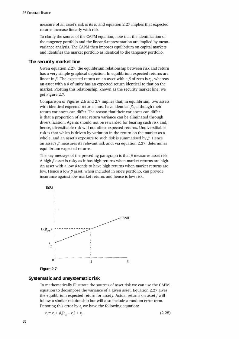
92 Corporate finance
36
measure of an asset’s risk is its β, and equation 2.27 implies that expected returns increase linearly with risk.
To clarify the source of the CAPM equation, note that the identification of the tangency portfolio and the linear β-representation are implied by mean–variance analysis. The CAPM then imposes equilibrium on capital markets and identifies the market portfolio as identical to the tangency portfolio.
The security market lineGiven equation 2.27, the equilibrium relationship between risk and return has a very simple graphical depiction. In equilibrium expected returns are linear in β. The expected return on an asset with a β of zero is rf , whereas an asset with a β of unity has an expected return identical to that on the market. Plotting this relationship, known as the security market line, we get Figure 2.7.
Comparison of Figures 2.6 and 2.7 implies that, in equilibrium, two assets with identical expected returns must have identical βs, although their return variances can differ. The reason that their variances can differ is that a proportion of asset return variance can be eliminated through diversification. Agents should not be rewarded for bearing such risk and, hence, diversifiable risk will not affect expected returns. Undiversifiable risk is that which is driven by variation in the return on the market as a whole, and an asset’s exposure to such risk is summarised by β. Hence an asset’s β measures its relevant risk and, via equation 2.27, determines equilibrium expected returns.
The key message of the preceding paragraph is that β measures asset risk. A high β asset is risky as it has high returns when market returns are high. An asset with a low β tends to have high returns when market returns are low. Hence a low β asset, when included in one’s portfolio, can provide insurance against low market returns and hence is low risk.
Figure 2.7
Systematic and unsystematic riskTo mathematically illustrate the sources of asset risk we can use the CAPM equation to decompose the variance of a given asset. Equation 2.27 gives the equilibrium expected return for asset j. Actual returns on asset j will follow a similar relationship but will also include a random error term. Denoting this error by εj we have the following equation:
rj = rf + βj [rM – rf ] + εj. (2.28)

Chapter 2: Risk and return: mean–variance analysis and the CAPM
37
The variance of the risk-free return is zero by definition. Assuming that βj is fixed we can represent the variance of asset j as:
σ2j = β2
jσ2M + σ2
ε. (2.29)
The final term on the right-hand side of equation 2.29 is the variance of the error term and represents diversifiable risk. This source of risk is also known as unsystematic and idiosyncratic risk. As emphasised previously, this risk is unrelated to market fluctuations and, therefore, does not affect expected returns. The first term on the right-hand side of equation 2.29 represents undiversifiable risk, also known as systematic risk. This is risk that cannot be escaped and hence increases equilibrium expected returns.
Activities8
1. An investor forms a portfolio of two assets, X and Y. These assets have expected returns of 9 per cent and 6 per cent and standard deviations of 0.8 and 0.6 respectively. Assuming that the investor places a portfolio weight of 0.5 on each asset, calculate the portfolio expected return and variance if the correlation between returns on X and Y is unity.
2. Using the data from Question 1, recalculate the portfolio expected return and variance, assuming that the correlation between returns is 0.5.
3. An investor forms a portfolio from two assets, P and Q, using portfolio weights of one-third and two-thirds respectively. The expected returns on P and Q are 5 per cent and 7 per cent, and their respective return standard deviations are 0.4 and 0.5. Assuming that the return correlation is zero, calculate the expected return and variance of the investor’s portfolio.
4. Assuming identical data to that in Question 3, recalculate the statistical properties of the portfolio, assuming the return correlation for P and Q is –0.5.
The Roll critique and empirical tests of the CAPMThe final topic we touch on in this chapter is the empirical validity of the CAPM. The model of equilibrium expected returns that we have developed in the preceding sections of this chapter is obviously not guaranteed to hold in practice and, hence, rather than just blindly accepting its output, we should examine how it holds up when applied to real data. However, this task brings us face-to-face with a problem first pointed out by Richard Roll and hence known as the Roll critique.9
The statement of the CAPM is identical to the proposition that the market portfolio is mean–variance efficient. Hence, Roll pointed out that empirical tests of the CAPM should seek to examine whether this is indeed the case. However, he also noted that the market portfolio (or the return on the market) is not observable to an econometrician, who wishes to conduct a test. Empirical researchers generally use a broad-based equity index such as the FTSE-100, S&P-500 or Nikkei 250 to proxy the market. But the true market portfolio will contain other financial assets (such as bonds and stocks not included in such indices) as well as non-financial assets such as real estate, durable goods and even human capital. Hence, the validity of tests of the CAPM depend critically on the quality of the proxy used for the market portfolio.
Based on the above, Roll’s critique is simply that, due to the fact that the market portfolio is not observable, the CAPM is not testable. We can understand this through the following arguments. First, it might be the case that the market portfolio is efficient (and hence the CAPM is valid), but our chosen proxy for the market is not efficient, and hence our
8 You will fi nd the solutions to these activities at the end of this chapter.
9 See Roll (1977).
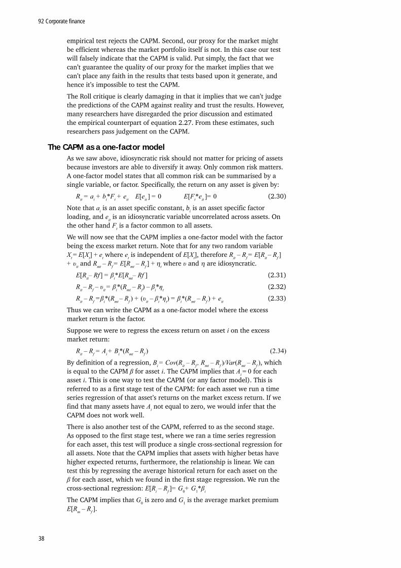
92 Corporate finance
38
empirical test rejects the CAPM. Second, our proxy for the market might be efficient whereas the market portfolio itself is not. In this case our test will falsely indicate that the CAPM is valid. Put simply, the fact that we can’t guarantee the quality of our proxy for the market implies that we can’t place any faith in the results that tests based upon it generate, and hence it’s impossible to test the CAPM.
The Roll critique is clearly damaging in that it implies that we can’t judge the predictions of the CAPM against reality and trust the results. However, many researchers have disregarded the prior discussion and estimated the empirical counterpart of equation 2.27. From these estimates, such researchers pass judgement on the CAPM.
The CAPM as a one-factor modelAs we saw above, idiosyncratic risk should not matter for pricing of assets because investors are able to diversify it away. Only common risk matters. A one-factor model states that all common risk can be summarised by a single variable, or factor. Specifically, the return on any asset is given by:
Rit = ai + bi*Ft + eit E[eit ] = 0 E[Ft*eit ]= 0 (2.30)
Note that ai is an asset specific constant, bi is an asset specific factor loading, and eit is an idiosyncratic variable uncorrelated across assets. On the other hand Ft is a factor common to all assets.
We will now see that the CAPM implies a one-factor model with the factor being the excess market return. Note that for any two random variable Xt = E[Xt] + et where et is independent of E[Xt], therefore Rit – Rf = E[Rit – Rf ] + υit and Rmt – Rf = E[Rmt – Rf ] + t where υ and are idiosyncratic.
E[Rit– Rf ] = βi*E[Rmt– Rf ] (2.31)
Rit – Rf – υit = βi*(Rmt – Rf) – βi*ηt (2.32)
Rit – Rf =βi*(Rmt – Rf ) + (υit – βi*ηt) = βi*(Rmt – Rf ) + eit (2.33)
Thus we can write the CAPM as a one-factor model where the excess market return is the factor.
Suppose we were to regress the excess return on asset i on the excess market return:
Rit – Rf = Ai + Bi*(Rmt – Rf ) (2.34)
By definition of a regression, Bi = Cov(Rit – Rf , Rmt – Rf )/Var(Rmt – Rf ), which is equal to the CAPM β for asset i. The CAPM implies that Ai = 0 for each asset i. This is one way to test the CAPM (or any factor model). This is referred to as a first stage test of the CAPM: for each asset we run a time series regression of that asset’s returns on the market excess return. If we find that many assets have Ai not equal to zero, we would infer that the CAPM does not work well.
There is also another test of the CAPM, referred to as the second stage. As opposed to the first stage test, where we ran a time series regression for each asset, this test will produce a single cross-sectional regression for all assets. Note that the CAPM implies that assets with higher betas have higher expected returns, furthermore, the relationship is linear. We can test this by regressing the average historical return for each asset on the β for each asset, which we found in the first stage regression. We run the cross-sectional regression: E[Ri – Rf ]= G0+ G1*βi
The CAPM implies that G0 is zero and G1 is the average market premium E[Rm – Rf ].

Chapter 2: Risk and return: mean–variance analysis and the CAPM
39
The data are generally not supportive of the CAPM. The relationship between an asset’s β and its average return is usually positive, as the CAPM suggests, but typically flatter than it should be, as can be seen in Figure 2.8. In this figure the β’s are plotted against average returns for 17 portfolios based on industry (such as food, chemicals or transportation). The dotted line plots β against β*E[Rm – Rf ], this is the CAPM predicted expected return. The solid line plots the actual relationship between β and industry returns, this relationship is positive but flatter than the dotted line. That is high β stocks have returns that are lower than predicted by the CAPM while low β stocks have returns that are higher than predicted by the CAPM. Furthermore, there are certain assets (to be discussed in the next chapter) that appear to consistently have non-zero Ai in time series regressions.10
0.7 0.8 0.9 1 1.1 1.2 1.3 1.40.4
0.45
0.5
0.55
0.6
0.65
0.7
0.75
0.8
0.85
0.9
β
E[R]
Figure 2.8
One possible explanation for the too flat relationship between β and average return is measurement error. Suppose we do not observe an asset’s true β, but rather its true β plus some measurement error which is mean zero. Then assets with very high observed β are likely to be assets with very positive measurement error; therefore their true β is below their observed β, perhaps consistent with the low observed expected return. Similarly, assets with very low observed β are likely to be assets with very negative measurement error and therefore their true β is above the observed β.
It is also possible that one factor is simply not enough to explain all of the variation in expected returns. The CAPM implies that the a firm’s loading on the market (β) is the only variable that should cause expected returns to differ. Adding extra explanatory variables to regression 2.34 will not result in significant coefficients. In the next chapter we will see that loadings on other factors, including firm size, book-to-market ratios, P/E ratios and dividend yields have been shown to explain ex-post realised returns.
Amalgamating the above evidence implies that, if you are willing to disregard the Roll critique, you should probably conclude that the CAPM does not hold. This has led certain authors to investigate other asset-pricing pradigms such as the APT (which we discuss in the next chapter). An alternative viewpoint would be to argue that such results tell us little or nothing about the validity of the CAPM due to the insight of Roll (1977).
10 See pp.185–86 of Brealey and Myers (2008).

92 Corporate finance
40
A reminder of your learning outcomesHaving completed this chapter, and the Essential reading and activities, you should be able to:
• discuss concepts such as a portfolio’s expected return and variance as well as the covariance and correlation between portfolios’ returns
• calculate portfolio expected return and variance from the expected returns and return variances of constituent assets with confidence
• describe the effects of diversification on portfolio characteristics
• derive the CAPM using mean–variance analysis
• describe some theoretical and practical limitations of the CAPM.
Key termsbeta (β)capital asset pricing model (CAPM)
correlation
covariance
diversification
expected return
market portfolio
mean–variance analysis
Roll critique
security market line
standard deviation
systematic risk
two-fund separation
unsystematic risk
variance
Sample examination questions1. Detail the assumptions that underlie the CAPM and provide a
derivation of the CAPM equation. Support your derivation with graphical evidence. (15%)
2. The returns on ABC stock and on the market portfolio in three consecutive years are given in the following table:
Year ABC return (%) Market return (%)
1 8 6
2 24 12
3 28 15
Showing all your workings, compute the β for ABC’s equity. (7%)
4. Assume that the risk-free rate is 5 per cent. What is the expected return on ABC’s stock? (3%)
5. The risk-free rate is 4 per cent, firm A has a market β of 2 and an expected return of 16 per cent.
a. What is the expected return on the market according to the CAPM?

Chapter 2: Risk and return: mean–variance analysis and the CAPM
41
b. Draw a graph with β on the x-axis and the expected return on the y-axis. Indicate the risk-free rate, the market, and firm A. What is the slope of the securities market line?
c. The standard deviation of the market return is 16 per cent and the standard deviation of the return of firm A is 40 per cent. What is the standard deviation of A’s idiosyncratic component?
6. You have 50 years of monthly data on short-term treasury rates and portfolios of 10-year bond returns, an aggregate index of US equities, a mutual fund focusing on tech firms, a mutual fund focusing on commodities, a mutual fund focusing on manufacturing, and a hedge fund index. Describe how you would test the CAPM and the results you would expect to find.
Solutions to activities1. The expected return on the equally weighted portfolio is 7.5 per cent.
The portfolio return variance is 0.49, and hence the portfolio return standard deviation is 0.7.
2. Obviously, the expected return is the same as in Question 1. With correlation of 0.5, the portfolio return variance is 0.37.
3. The expected return on the portfolio is 6.33 per cent, and the portfolio has a return variance of 0.1289.
4. When the correlation changes to –0.5, the portfolio return variance drops to 0.0844. The expected return on the portfolio doesn’t change from that calculated in Question 3.

Notes
92 Corporate finance
42

Chapter 3: Factor models
43
Chapter 3: Factor models
Aim of the chapterThe aim of this chapter is to derive arbitrage pricing theory, an alternative to the capital asset pricing model, enabling us to price financial assets.
Learning outcomesBy the end of this chapter, and having completed the Essential reading and activities, you should be able to:
• understand single-factor and multi-factor model representations
• derive factor-replicating portfolios from a set of asset returns
• understand the notion of arbitrage strategies and that well-functioning financial markets should be arbitrage-free
• derive arbitrage pricing theory and calculate expected returns using the pricing formulas
• know how to test multifactor models.
Essential readingHillier, D., M. Grinblatt and S. Titman Financial Markets and Corporate Strategy.
(Boston, Mass.; London: McGraw-Hill, 2008) Chapter 6 (Factor Models and the APT).
Further readingBrealey, R., S. Myers and F. Allen Principles of Corporate Finance. (Boston,
Mass.; London: McGraw-Hill, 2008) Chapter 9 (Risk and Return).Chen, N-F. ‘Some empirical tests of the theory of arbitrage pricing’, The Journal
of Finance 38(5) 1983, pp.1393–414.Chen, N-F., R. Roll and S. Ross ‘Economic forces and the stock market’, Journal
of Business 59 1986, pp.383–403.Copeland, T., J. Weston and K. Shastri Financial Theory and Corporate Policy.
(Reading, Mass.; Wokingham: Addison-Wesley, 2005) Chapter 6.Fama, E. and K. French ‘The cross-section of expected stock returns’, Journal of
Finance 47(2) 1992, pp.427–65.Fama, E. and K. French ‘Common risk factors in the returns on stocks and
bonds’, Journal of Financial Economics 33 1993, pp.3–56.Fama, E. and J. MacBeth ‘Risk, return, and equilibrium: empirical tests’, Journal
of Political Economy 91 1973, pp.607–36.Gibbons, M.R., S.A. Ross and J. Shanken ‘A test of the efficiency of a given
portfolio’, Econometrica 57 1989, pp.1121–52.Jegadeesh, N. and S. Titman ‘Returns to buying winners and selling losers’,
Journal of Finance 48 1993.
OverviewEmpirically, expected returns appear to depend on several factors. For this reason, multifactor models, such as the Fama and French three-factor model are commonly used in practice to calculate expected returns. The arbitrage pricing theory gives a theoretical basis for using such models. As its name suggests, it rests on the notion that well-functioning financial markets should be arbitrage-free. This, using a factor model of asset
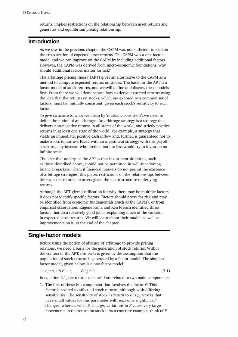
92 Corporate finance
44
returns, implies restrictions on the relationship between asset returns and generates and equilibrium pricing relationship.
IntroductionAs we saw in the previous chapter, the CAPM was not sufficient to explain the cross-section of expected asset returns. The CAPM was a one-factor model and we can improve on the CAPM by including additional factors. However, the CAPM was derived from micro-economic foundations, why should additional factors matter for risk?
The arbitrage pricing theory (APT) gives an alternative to the CAPM as a method to compute expected returns on stocks. The basis for the APT is a factor model of stock returns, and we will define and discuss these models first. From there we will demonstrate how to derive expected returns using the idea that the returns on stocks, which are exposed to a common set of factors, must be mutually consistent, given each stock’s sensitivity to each factor.
To give structure to what we mean by ‘mutually consistent’, we need to define the notion of an arbitrage. An arbitrage strategy is a strategy that delivers non-negative returns in all states of the world, and strictly positive returns in at least one state of the world. For example, a strategy that yields an immediate, positive cash inflow and, further, is guaranteed not to make a loss tomorrow. Faced with an investment strategy with this payoff structure, any investor who prefers more to less would try to invest on an infinite scale.
The idea that underpins the APT is that investment situations, such as those described above, should not be permitted in well-functioning financial markets. Then, if financial markets do not permit the existence of arbitrage strategies, this places restrictions on the relationships between the expected returns on assets given the factor structure underlying returns.
Although the APT gives justification for why there may be multiple factors, it does not identify specific factors. Factors should proxy for risk and may be identified from economic fundamentals (such as the CAPM), or from empirical observation. Eugene Fama and Ken French identified three factors that do a relatively good job at explaining much of the variation in expected stock returns. We will learn about their model, as well as improvements on it, at the end of the chapter.
Single-factor modelsBefore using the notion of absence of arbitrage to provide pricing relations, we need a basis for the generation of stock returns. Within the context of the APT, this basis is given by the assumption that the population of stock returns is generated by a factor model. The simplest factor model, given below, is a one-factor model:
ri = αi + βi F + εi E(εi) = 0. (3.1)
In equation 3.1, the returns on stock i are related to two main components:
1. The first of these is a component that involves the factor F. This factor is posited to affect all stock returns, although with differing sensitivities. The sensitivity of stock i’s return to F is βi. Stocks that have small values for this parameter will react only slightly as F changes, whereas when βi is large, variations in F cause very large movements in the return on stock i. As a concrete example, think of F
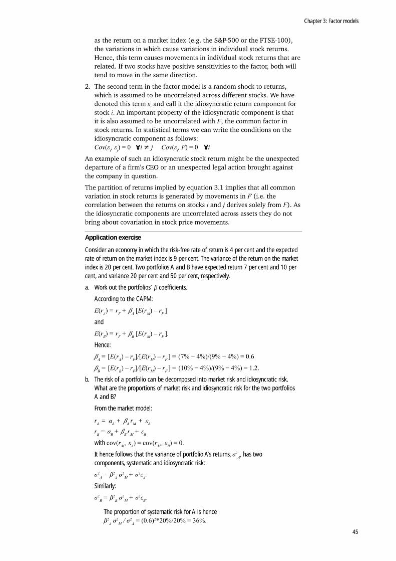
Chapter 3: Factor models
45
as the return on a market index (e.g. the S&P-500 or the FTSE-100), the variations in which cause variations in individual stock returns. Hence, this term causes movements in individual stock returns that are related. If two stocks have positive sensitivities to the factor, both will tend to move in the same direction.
2. The second term in the factor model is a random shock to returns, which is assumed to be uncorrelated across different stocks. We have denoted this term εi and call it the idiosyncratic return component for stock i. An important property of the idiosyncratic component is that it is also assumed to be uncorrelated with F, the common factor in stock returns. In statistical terms we can write the conditions on the idiosyncratic component as follows:Cov(εi, εj) = 0 i ≠ j Cov(εi, F) = 0 i
An example of such an idiosyncratic stock return might be the unexpected departure of a firm’s CEO or an unexpected legal action brought against the company in question.
The partition of returns implied by equation 3.1 implies that all common variation in stock returns is generated by movements in F (i.e. the correlation between the returns on stocks i and j derives solely from F). As the idiosyncratic components are uncorrelated across assets they do not bring about covariation in stock price movements.
Application exercise
Consider an economy in which the risk-free rate of return is 4 per cent and the expected rate of return on the market index is 9 per cent. The variance of the return on the market index is 20 per cent. Two portfolios A and B have expected return 7 per cent and 10 per cent, and variance 20 per cent and 50 per cent, respectively.
a. Work out the portfolios’ β coefficients.
According to the CAPM:
E(rA) = rF + βA [E(rM) – rF ]
and
E(rB) = rF + βB [E(rM) – rF ].
Hence:
βA = [E(rA) – rF]/[E(rM) – rF ] = (7% − 4%)/(9% − 4%) = 0.6
βB = [E(rB) – rF]/[E(rM) – rF ] = (10% − 4%)/(9% − 4%) = 1.2.
b. The risk of a portfolio can be decomposed into market risk and idiosyncratic risk. What are the proportions of market risk and idiosyncratic risk for the two portfolios A and B?
From the market model:
rA = αA + βA rM + εA
rB = αB + βB rM + εB
with cov(rM , εA) = cov(rM , εB) = 0.
It hence follows that the variance of portfolio A’s returns, σ2A, has two
components, systematic and idiosyncratic risk:
σ2A = β2
A σ2M + σ2εA.
Similarly:
σ2B = β2
B σ2M + σ2εB.
The proportion of systematic risk for A is hence β2
A σ2M / σ2
A = (0.6)2*20%/20% = 36%.
A A
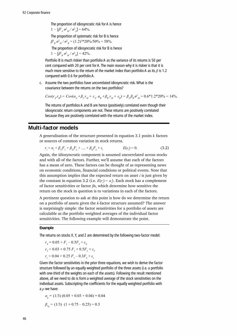
92 Corporate finance
46
The proportion of idiosyncratic risk for A is hence 1 − [β2
A σ2M / σ2
A] = 64%.
The proportion of systematic risk for B is hence β2
B σ2M / σ2
B = (1.2)2*20%/50% = 58%.
The proportion of idiosyncratic risk for B is hence 1 − [β2
B σ2M / σ2
B] = 42%.
Portfolio B is much riskier than portfolio A as the variance of its returns is 50 per cent compared with 20 per cent for A. The main reason why it is riskier is that it is much more sensitive to the return of the market index than portfolio A as its β is 1.2 compared with 0.6 for portfolio A.
c. Assume the two portfolios have uncorrelated idiosyncratic risk. What is the covariance between the returns on the two portfolios?
Cov(rA,rB) = Cov(αA +βA rM + εA, αB +βB rM + εB) = βA βB σ2
M = 0.6*1.2*20% = 14%.
The returns of portfolios A and B are hence (positively) correlated even though their idiosyncratic return components are not. These returns are positively correlated because they are positively correlated with the returns of the market index.
Multi-factor modelsA generalisation of the structure presented in equation 3.1 posits k factors or sources of common variation in stock returns.
ri = αi + β1iF1 + β2iF2 + .... + βkiFk + εi E(εi) = 0. (3.2)
Again, the idiosyncratic component is assumed uncorrelated across stocks and with all of the factors. Further, we’ll assume that each of the factors has a mean of zero. These factors can be thought of as representing news on economic conditions, financial conditions or political events. Note that this assumption implies that the expected return on asset i is just given by the constant in equation 3.2 (i.e. E(ri) = αi). Each stock has a complement of factor sensitivities or factor βs, which determine how sensitive the return on the stock in question is to variations in each of the factors.
A pertinent question to ask at this point is how do we determine the return on a portfolio of assets given the k-factor structure assumed? The answer is surprisingly simple: the factor sensitivities for a portfolio of assets are calculable as the portfolio weighted averages of the individual factor sensitivities. The following example will demonstrate the point.
Example
The returns on stocks X, Y, and Z are determined by the following two-factor model:
rX = 0.05 + F1 – 0.5F2 + εX
rY = 0.03 + 0.75 F1 + 0.5F2 + εY
rz = 0.04 + 0.25 F1 – 0.3F2 + εz
Given the factor sensitivities in the prior three equations, we wish to derive the factor structure followed by an equally weighted portfolio of the three assets (i.e. a portfolio with one-third of the weights on each of the assets). Following the result mentioned above, all we need to do is form a weighted average of the stock sensitivities on the individual assets. Subscripting the coefficients for the equally weighted portfolio with a p we have:
αp = (1/3) (0.05 + 0.03 + 0.04) = 0.04
β1p = (1/3) (1 + 0.75 – 0.25) = 0.5
Chapter 3: Factor models
47
β2p = (1/3) (–0.5 + 0.5 – 0.3) = –0.1
and hence; the factor representation for the portfolio return can be written as:
rp = 0.04 + 0.5F1 – 0.1F2 + εp
where the final term is the idiosyncratic component in the portfolio return. Note that the idiosyncratic volatility of the portfolio is εp = (1/3)(εX + εY + εz) smaller than the idiosyncratic volatilities of portfolios X, Y or Z because the idiosyncratic components are independent.
Activity
Using the data given in the previous example, compute the return representation for a portfolio of assets X, Y and Z with portfolio weights –0.25, 0.5 and 0.75.
An important implication of the result is the following. Assume a two-factor model, and also assume that we are given the factor representations for three stocks. I can construct a portfolio of these three assets, which has any desired set of factor sensitivities through appropriate choice of the portfolio weights.1 What underlies this result? Well, to illustrate let’s use the data from the prior example. Assume I wish to construct a portfolio with a sensitivity of 0.5 on the first factor and a sensitivity of 1 on the second factor. Denoting the portfolio weights on the individual assets by ωX, ωY and ωZ it must be the case that:
ωX + 0.75ωY – 0.25ωZ = 0.5 (3.3)
–0.05ωX + 0.5ωY – 0.3ωZ = 1. (3.4)
Finally, it must also be the case that the portfolio weights add up to unity, so we must also satisfy the following equation:
ωX + ωY + ωZ = 1.
Equations 3.3, 3.4 and 3.5 are three equations in three unknowns, and we can find values for the portfolio weights which satisfy all three simultaneously. This illustrates the fact that (as the portfolio factor sensitivities were arbitrarily set at 0.5 and 1) we can derive any constellation of factor sensitivities. A particularly interesting case is when the portfolio is sensitive to one of the factors only. We call this a factor-replicating portfolio and discuss it below.
Broad-based portfolios and idiosyncratic returnsIn what follows we will assume that the basic securities that we’re going to work with are themselves broad-based portfolios. The reason for thisis that it allows us to lose the idiosyncratic risk terms associated with single stocks. Why is this the case? Well, consider the idiosyncratic risk term for an equally weighted portfolio of 100 stocks. Call the ith idiosyncratic term εi and assume that all idiosyncratic terms have variance σ2. The variance of the idiosyncratic element of the portfolio return is then:
y y .
Note that, under these assumptions the variance of the idiosyncratic portfolio return is only one-hundredth of the variance of any individual asset’s idiosyncratic return. In a general case, where one forms an equally weighted portfolio of n assets, the variance of the idiosyncratic term for the portfolio return is n-1σ2. This is a diversification result just like those we used in Chapter 2. The fact that the idiosyncratic returns are uncorrelated with one another means that their influence tends to disappear when one groups assets into large portfolios.
1 In general, if I have a k-factor model I will need k+1 stocks to do this.
92 Corporate finance
48
Factor-replicating portfoliosAn important application of the technology developed previously in this chapter is the construction of a factor-replicating portfolio. A factor-replicating portfolio is a portfolio with unit exposure to one factor and zero exposure to all others. For example, the portfolio replicating factor 1 in model 3.2 would have β1 = 1 and βj = 0 for all j = 2 to k. We will use factor-replicating portfolios to show that a factor structure for asset returns implies a β pricing model. In such a model, expected returns depend only on βs, or risk loadings.
Activity
Assume that stock returns are generated by a two-factor model. The returns on three well-diversified portfolios, A, B and C, are given by the following representations:
rA = 0.10 + F1 – 0.5F2
rB = 0.08 + 2F1 + F2
rC = 0.05 + 0.5F1 + 0.5F2.
Determine the portfolio weights you need to place on A, B and C in order to construct the two factor-replicating portfolios plus a portfolio which has zero exposure to both factors. What are the expected returns of the factor-replicating portfolios and what is the expected return of the risk-free portfolio?
The question to ask at this point is: why bother constructing factor-replicating portfolios? The reason is as follows. Suppose I want to build a portfolio that has identical factor exposures to a given asset, X. Assume a two-factor world and that asset X has exposure of 0.75 to factor 1 and –0.3 to factor 2. Assume also that I know the two factor-replicating portfolios.
Building a portfolio with the same factor exposures as X is now simple. Construct a new portfolio, Y, which has portfolio weight 0.75 on the replicating portfolio for the first factor, portfolio weight –0.3 on the replicating portfolio for the second factor and the rest of the portfolio weight (i.e. a weight of 1 – 0.75 + 0.3 = 0.55) on the risk-free asset. Via the results on the factor representations of a portfolio of assets and the definition of a factor-replicating portfolio it is easy to see that Y is guaranteed to have identical factor exposures to X.
The replication in the preceding paragraph forms the basis for the APT. For absence of arbitrage we require all assets with identical factor exposures to earn the same return. If they did not, then we would have the chance to make unlimited amounts of money. For example, assume that the expected return on the replicating portfolio Y was greater than that on asset X. Then I should short X and buy Y. The risk exposures of the two portfolios are identical and hence risks cancel out and I am left with an excess return that is riskless (i.e. an arbitrage gain).
In order to progress, let us introduce some notation. Denote the risk-free rate with rf. Denote the expected return on the ith factor-replicating portfolio with rf + λi such that λi is the risk premium associated with the ith factor. Again, for simplicity, assume that the world is generated by a two-factor model, and assume that I wish to replicate asset X, which has sensitivity β1X to the first factor and β2X to the second factor. Finally, we will assume that the primary securities being worked with are well-diversified portfolios themselves. Hence, we will ignore any idiosyncratic risk in this derivation.

Chapter 3: Factor models
49
Using the prior argument, to replicate asset X’s factor sensitivities, we construct a portfolio with weight β1X on the first factor-replicating portfolio, weight β2X on the second factor-replicating portfolio and weight 1 – β1X – β2X
on the risk-free asset. The expected return of the replicating portfolio is hence:
β1X (rf + λ1) + β2X (rf + λ2) + (1 – β1X – β2X) rf = rf + β1X λ1+ β2X λ2. (3.6)
Hence, using our factor-replicating portfolios we can write the expected return on a portfolio which replicates X’s factor exposures as the risk-free rate plus each factor exposure multiplied by the risk premium on the relevant factor-replicating portfolio.
Note that equation 3.6 can be used to test the factor model. This is the second stage test of factor models mentioned in the previous chapter in the context of the CAPM. Equation 3.6 states that average returns on assets are higher if those assets have higher factor loadings (βs); the factors are the same for all assets. This is a cross-sectional statement as it compares average returns for different assets. We can regress average returns on assets in excess of rf on the historical βs of these assets (here β is the regressor, not the coefficient). If the factor model performs well then the intercept of this regression should be close to zero.
The reason this regression is called a second stage regression is because we must first find βs by running a time series regression for each asset on the factor mimicking portfolios. These regressions can also be used to test the factor model, these are called first stage tests. We can use equation 3.6 to derive this equation as well. Combine equations 3.2 and 3.6 by noting that the i in equation 3.6 is the expected return on asset i, given by equation 3.2:
rit= (rf + β1i λ1 + β2i λ2 ) + β1i F1t + β2i F2t + εit (3.7)
rit – rf = β1i (λ1 +F1t )+β2i (λ2 + F2t ) + εit = β2t(λ1 + F1t ) + β2i(λ2 + F2t ) + εit , (3.8)
where j+Fjt is the excess return on the jth factor-replicating portfolio (plus some idiosyncratic risk if markets are incomplete). Thus a time series regression of rit – rf on excess factor returns implies that the intercept must be zero; this must be true for each asset.
A practical question is how close to zero must the intercept be in both the first and second stages in order for us to accept a model as being ‘close’ to the data? Consider the first stage which states that every asset must have a zero intercept. Suppose we found that 15 out of 100 tested assets had intercepts different from zero at 5 per cent significance. A naïve application of statistics would suggest rejection of the factor model. However, rejection is not as clear cut as it might appear.
Suppose you were told that one of the assets with a non-zero intercept was McDonalds. It would then not be surprising if we also found Burger King to have a non-zero intercept because the two are likely to be highly correlated even when controlling for standard factors. The 100 tested assets may not all be truly independent and we are likely to see highly correlated assets both be rejected or both not be rejected. If the 15 assets that are rejected are all highly correlated, while the remaining 85 are not, we should not reject the model. Gibbons, Ross and Shanken (1989) provide a procedure to test the intercepts jointly for many assets, some of which are potentially correlated.
Let us now turn to the second stage test which also states that the intercept (this time in a cross-sectional regression) must be zero. We can check for the significance of the intercept in the usual way. However, when doing
92 Corporate finance
50
this we are implicitly making an assumption about the cross-sectional distribution of returns. Fama and MacBeth (1973) suggested an alternative implementation of the second stage test which avoids making such assumptions. Instead of running a single regression of average historical returns on historical βs they suggest running a separate regression each year; for each year regress the realised returns on βs calculated over some recent period. As a result for each year there will be a separate estimate of the intercept. They suggest using the distribution of intercepts to calculate significance.
The arbitrage pricing theoryConsider an arbitrary asset. The previous subsection tells us that it’s simple to replicate this asset’s risk (i.e. its factor exposures) using factor-replicating portfolios. The key to the APT is that absence of arbitrage requires that such a pair of portfolios must have identical expected returns in a financial market equilibrium. If they did not, it would be possible to make unlimited amounts of money without incurring any risk.
This implies that the expected return on asset X, rX, must be identical to the expression arrived at in equation 3.6, that is:
E(rX) = rf + β1X λ1+ β2X λ2. (3.9)
Equation 3.7 is the statement of the APT. The expected return on a financial asset can be written as the risk-free rate plus sum of the asset’s factor sensitivities multiplied by the factor-risk premiums (which are invariant across assets). If such an expression does not hold at all times, arbitrage opportunities exist. Note the assumptions that are required to achieve this result. First, we require that asset returns are generated by a two-factor (or in general k-factor) model. Second, we assume that arbitrage opportunities cannot exist. Lastly, we assume that enough assets are available such that firm-specific risk washes away when portfolios are formed.
Example
In the previous two-factor example, we determined the expected returns on the two factor-replicating portfolios. Denoting the expected return on the ith factor-replicating portfolio by E(ri) we have:
E(r1) = 8.29% E(r2) = 1.71% E(r3) = 5.14%.
Hence, the premiums associated with the two factors are:
λ1 = 8.29 – 5.14 = 3.15%, λ2 = 1.71 – 5.14 = 3.43%.
This implies that the expected return on any asset in this world can be written as:
E(ri) = 5.14 + 3.15β1i – 3.43β2i .
To check that this works, substitute (for example) portfolio C’s factor sensitivities into the preceding expression. This gives:
E(rC) = 5.14 + 3.15 (0.5) – 3.43 (0.5) = 5%,
and hence, agrees with the expected return implied by the original representation for asset C. Check that the expected returns on assets A and B also come out correctly.
To analyse an arbitrage opportunity that might arise in markets, attempt the following activity.

Chapter 3: Factor models
51
Activity
Assume that a new well-diversified portfolio, D, is added to our world. This asset has sensitivities of 3 and –1 to the two factors and an expected return of 15 per cent.
Using the equilibrium expected return equation given above, derive the equilibrium expected return on an asset with identical factor exposures to D. Is there now an arbitrage opportunity available? If so, dictate a strategy that could be employed to exploit the arbitrage opportunity.
Multi-factor models in practiceAs discussed earlier, the CAPM is a one-factor model where the only factor is the excess market return. Securities with higher loading (β) on the market return should have higher expected returns; nothing else should matter for expected returns. Furthermore, the α of each security should be zero.
Eugene Fama and Ken French illustrated the failure of the CAPM by forming portfolios of securities in a particular way. First, for each security they calculated the firm’s size (market cap) and its market-to-book ratio (a ratio of the firm’s market value to its book value). They then formed cut-offs based on size and book-to-market, and assigned firms to one of five quintiles for each trait. This resulted in 25 different portfolios (i.e. large size and small book-to-market, small size and medium size book-to-market, etc.), this is called a double sort. Once a year the portfolios would be updated to take into account any changes to firm characteristics.
Fama and French showed that portfolios of small firms tended to have larger returns than portfolios of large firms, portfolios of high book-to-market (value) firms tended to have larger returns than portfolios of low book-to-market (growth) firms. Interestingly, these patterns remained even once controlling for market risk.
Recall that the first stage test of the CAPM implies that for any asset or portfolio, a regression of that asset’s returns on the market should have an intercept (α) of zero. Portfolios of small firms and value firms had positive α implying their returns were higher than predicted by the CAPM, conversely portfolios of large and growth firms had negative αs implying their returns were lower than predicted by the CAPM. This is evident in Table 3.1, which shows CAPM αs for portfolios double sorted on size and book-to-market.
Growth 2 3 4 Value
Small –0.573 –0.105 0.151 0.362 0.528
2 –0.213 0.146 0.295 0.312 0.363
3 –0.136 0.160 0.262 0.291 0.276
4 0.005 0.049 0.156 0.209 0.163
Big –0.014 0.022 0.038 –0.013 –1.020
Table 3.1
Since the CAPM could not adequately explain the cross-section of returns, Fama and French looked for additional risk factors. Given the performance of small and value stocks, it was natural to think those two characteristics were related to risk. They constructed a zero cost portfolio which took a long position in small stocks and a short position in large stocks and called it SMB (small minus big). Similarly, they constructed a zero cost portfolio which took a long position in value stocks and a short position in growth stocks and called it HML (high minus low).
92 Corporate finance
52
Fama and French augmented the CAPM by these two additional factors, creating what is known as the Fama and French three-factor model. As before with the CAPM, multifactor models can be tested by a first stage time series test, in which each asset’s return is regressed on the factors; each should be near zero. The Fama and French three-factor model performed much better than the CAPM on the 25 portfolios defined above, Fama and French could not statistically reject that the 25 αs were different from zero. The Fama and French model is commonly used as a replacement to the CAPM to assess risk as well as managerial performance.
Narasimhan Jegadeesh and Sheridan Titman found another set of portfolios whose returns could not be explained by the CAPM or the Fama and French three-factor model. Jegadeesh and Titman sorted stocks into portfolios based on their past performance, they held these portfolios for a year and then reassigned stocks to new portfolios. They found that a portfolio long in stocks that performed well in the past, and short in stocks that performed poorly in the past, had positive αs in both CAPM and three-factor regressions, they called this portfolio MOM (momentum). The momentum factor was added to the Fama and French three-factor model by Mark Carhart. This augmented four-factor model does a somewhat better job than the three-factor model at explaining the cross-section of expected stock returns, it is also commonly used to assess risk and managerial performance.
SummaryThe APT gives us a straightforward, alternative view of the world from the CAPM. The CAPM implies that the only factor that is important in generating expected returns is the market return and, further, that expected stock returns are linear in the return on the market. The APT allows there to be k sources of systematic risk in the economy. Some may reflect macroeconomic factors, like inflation, and interest rate risk, whereas others may reflect characteristics specific to a firm’s industry or sector.
Empirical research has indicated that some of the well-known empirical problems with the CAPM are driven by the fact that the APT is really the proper model of expected return generation. Chen (1983), for example, argues that the size effect found in CAPM studies disappears in a multi-factor setting. Chen, Roll and Ross (1986) argue that factors representing default spreads, yield spreads and gross domestic product growth are important in expected return generation. Fama and French (1992, 1995), show that size and book-to-market factors can help explain the cross-section of stock returns while other factors, such as momentum, also appear to be important. Work in this area is still progressing.
A reminder of your learning outcomesHaving completed this chapter, and the Essential reading and activities, you should be able to:
• understand single-factor and multi-factor model representations
• derive factor-replicating portfolios from a set of asset returns
• understand the notion of arbitrage strategies and that well-functioning financial markets should be arbitrage-free

Chapter 3: Factor models
53
• derive arbitrage pricing theory and calculate expected returns using the pricing formulas
• know how to test multifactor models.
Key termsarbitrage pricing theory
factor-replicating portfolio
factor sensitivity
multi-factor model
single-factor model
Sample examination question1. Assume that stock returns are generated by a two-factor model. The
returns on three well-diversified portfolios, A, B and C, are given by the following representations:
rA = 0.10 + F1
rB = 0.08 + 2F1 – F2
rC = 0.05 – 0.5F1 + 0.5F2
a. Discuss what the factor representations above imply for the variation and comovement in the three stock returns. Show how the returns of the stocks should be correlated between themselves.
b. Find the portfolio weights that one must place on stocks A, B and C to construct pure tracking portfolios for the two factors (i.e. portfolios in which the loading on the relevant factor is +1 and the loadings on all other factors are 0).
c. If one was to introduce a new portfolio, D, with loadings of +1 on both of the factors, what would the expected return on D have to be to rule out arbitrage?
d. Explain the concepts of idiosyncratic risk and factor risk in the APT. What role does diversification play in the APT?
2. Explain the first and second stage tests of factor models. Discuss how you would look for significance.
3. Explain how Fama and French form their portfolios and factors. What does it mean for a factor model to work well? What is Fama and French’s explanation for why their factor model works well?

Notes
92 Corporate finance
54