correlation between compaction characteristics with
TRANSCRIPT

Correlation between Compaction Characteristicswith undrained Shear Strength of Soils found inBurayu TownSOLOMON KORMU
AMBO UNIVERSITY WOLISO CAMPUS https://orcid.org/0000-0002-6143-6815Alemineh Sorsa ( [email protected] )
Jimma University
Research Article
Keywords: clay soils, Compaction, Correlation, undrained shear strength
Posted Date: October 7th, 2021
DOI: https://doi.org/10.21203/rs.3.rs-958664/v1
License: This work is licensed under a Creative Commons Attribution 4.0 International License. Read Full License

Jimma University
Jimma Institute of Technology
School of Graduate Studies
Faculty of Civil and Environmental Engineering
Geotechnical Engineering Stream
Correlation between Compaction Characteristics with undrained Shear
Strength of Soils found in Burayu Town
A Thesis Submitted to School of Graduate Studies of Jimma University in Partial
Fulfilment of the Requirement of Degree of Master of Science in Civil Engineering
(Geotechnical Engineering).
By:
Solomon Kormu
November, 2018
Jimma, Ethiopia

`
Jimma University
Jimma Institute of Technology
School of Graduate Studies
Faculty of Civil and Environmental Engineering
Geotechnical Engineering Stream
Correlation between Compaction Characteristics with undrained Shear
Strength of Soils found in Burayu Town
A Thesis Submitted to School of Graduate Studies of Jimma University in Partial
Fulfilment of the Requirement of Degree of Master of Science in Civil Engineering
(Geotechnical Engineering).
By:
Solomon kormu
Main advisor: Prof. Emer T. Quezon, P. Eng
Co-advisor: Engr. Alemneh Sorisa (PhD Candidate)
November, 2018
Jimma Ethiopia
`
Jimma University
Jimma Institute of Technology
School of Graduate Studies
Faculty of Civil and Environmental Engineering
Geotechnical Engineering Stream
Correlation between Compaction Characteristics with undrained Shear
Strength of Soils found in Burayu Town
By
Solomon Kormu
APPROVED BY BOARD OF EXAMINERS
1. ____________________________ ____________ ____/_____/____
External Examiner Signature Date
2. ____________________________ ____________ ____/_____/____
Internal Examiner Signature Date
3. ____________________________ ____________ ____/_____/____
Chairman of Examiner Signature Date
4. Prof. Emer T. Quezon, P.Eng ____ _____________ ____/_____/____
Main Advisor Signature Date
5. Alemneh Sorsa, MSc _____________ ____/_____/____
Co- Advisor Signature Date

i
DECLARATION
I, the undersigned, declare that this thesis entitled: “Correlation between Compaction
Characteristics with undrained Shear Strength of Soils found in Burayu Town” is my
original work, and has not been presented by any other person for an award of a degree in
this or any other University, and all sources of material used for this thesis have been duly
acknowledged.
Candidate:
Solomon Kormu
Signature
As Master’s Research Advisors, we hereby certify that we have read and evaluated this
MSc Thesis prepared under our guidance by Solomon Kormu entitled: “Correlation
between Compaction Characteristics with undrained Shear Strength of Soils found in
Burayu Town”.
We recommend that it can be submitted as fulfilling the MSc Thesis requirements.
23/11/2018
Prof. Emer T. Quezon, P.Eng ____________ _________
Advisor Signature Date
Engr. Alemneh Sorsa, MSc ____________ _________
Co- Advisor Signature Date

ii
ACKNOWLEDGEMENT
I would like to express sincere and special thanks to Prof. Emer T. Quezon, P.Eng, for his
continuous support, guidance, Lecturing and efforts in doing this Thesis. I would like to
thank Mr. Alemneh Sorisa for his genuine help. Special thanks to Jimma University and
Ethiopian road authority work at large glance in the country for Master Program.
I would like to thank my classmates, for a memorable friendly atmosphere, assistance and
invaluable comments. Finally, I would like to express my deepest gratitude to my parents,
my friends and all who contributed to this research work in one way or another.
iii
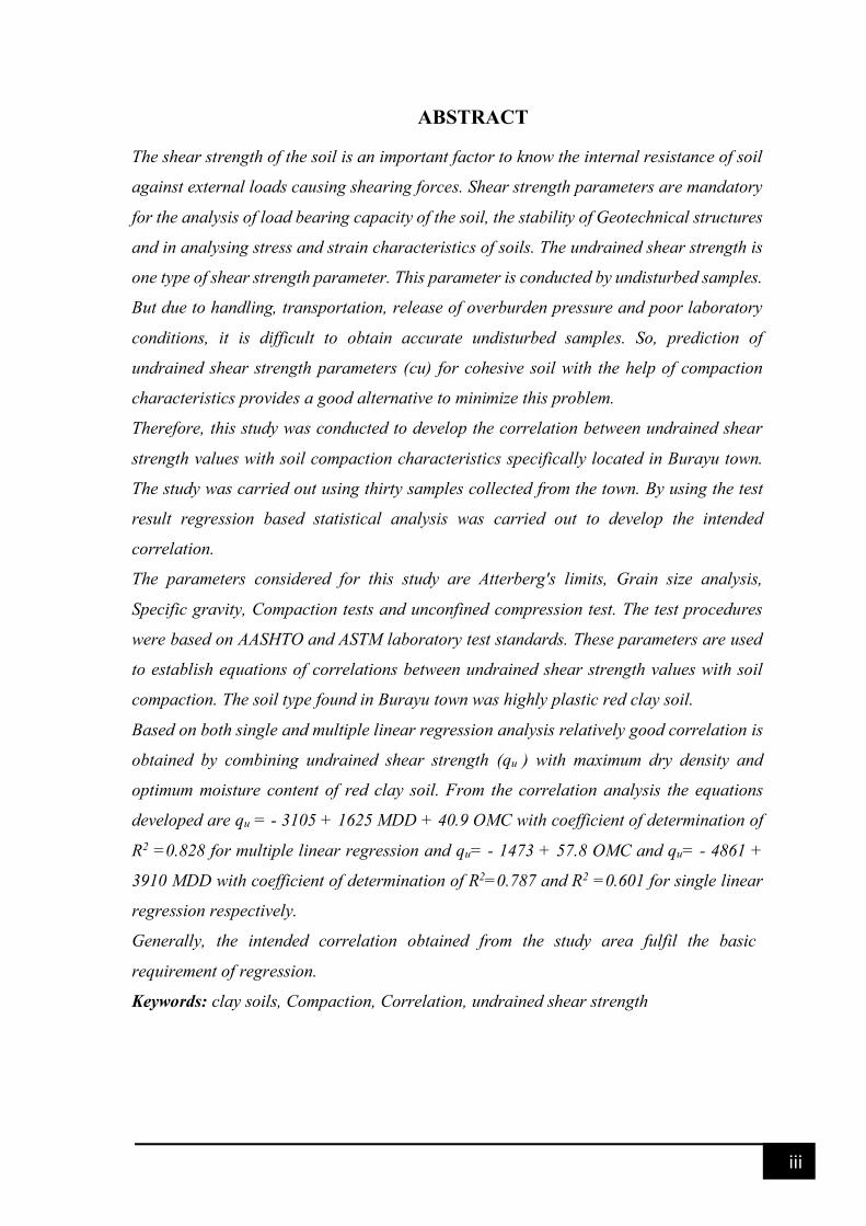
ABSTRACT
The shear strength of the soil is an important factor to know the internal resistance of soil
against external loads causing shearing forces. Shear strength parameters are mandatory
for the analysis of load bearing capacity of the soil, the stability of Geotechnical structures
and in analysing stress and strain characteristics of soils. The undrained shear strength is
one type of shear strength parameter. This parameter is conducted by undisturbed samples.
But due to handling, transportation, release of overburden pressure and poor laboratory
conditions, it is difficult to obtain accurate undisturbed samples. So, prediction of
undrained shear strength parameters (cu) for cohesive soil with the help of compaction
characteristics provides a good alternative to minimize this problem.
Therefore, this study was conducted to develop the correlation between undrained shear
strength values with soil compaction characteristics specifically located in Burayu town.
The study was carried out using thirty samples collected from the town. By using the test
result regression based statistical analysis was carried out to develop the intended
correlation.
The parameters considered for this study are Atterberg's limits, Grain size analysis,
Specific gravity, Compaction tests and unconfined compression test. The test procedures
were based on AASHTO and ASTM laboratory test standards. These parameters are used
to establish equations of correlations between undrained shear strength values with soil
compaction. The soil type found in Burayu town was highly plastic red clay soil.
Based on both single and multiple linear regression analysis relatively good correlation is
obtained by combining undrained shear strength (qu ) with maximum dry density and
optimum moisture content of red clay soil. From the correlation analysis the equations
developed are qu = - 3105 + 1625 MDD + 40.9 OMC with coefficient of determination of
R2 =0.828 for multiple linear regression and qu= - 1473 + 57.8 OMC and qu= - 4861 +
3910 MDD with coefficient of determination of R2=0.787 and R2 =0.601 for single linear
regression respectively.
Generally, the intended correlation obtained from the study area fulfil the basic
requirement of regression.
Keywords: clay soils, Compaction, Correlation, undrained shear strength

iv
TABLE OF CONTENTS
DECLARATION ............................................................................................................. i
ACKNOWLEDGEMENT ............................................................................................... ii
ABSTRACT................................................................................................................... iii
TABLE OF CONTENTS ............................................................................................... iv
LIST OF TABLES ........................................................................................................ vii
LIST OF FIGURES ...................................................................................................... viii
ABBREVIATIONS ........................................................................................................ ix
CHAPTER-ONE ............................................................................................................. 1
1 INTRODUCTION ................................................................................................... 1
1.1 Background ....................................................................................................... 1
1.2 Statement of the Problem .................................................................................. 1
1.3 Objectives of the Study ..................................................................................... 2
1.3.1 General Objectives ..................................................................................... 2
1.3.2 Specific Objectives .................................................................................... 3
1.4 Research Questions ........................................................................................... 3
1.5 Scope of the Study ............................................................................................ 3
1.6 Significance of the Study................................................................................... 4
1.7 Organization of the Thesis ................................................................................. 4
CHAPTER -TWO ............................................................................................................. 5
2 LITERATURE REVIEW............................................................................................ 5
2.1 Introduction....................................................................................................... 5
2.2 Shear Strength of Soils ...................................................................................... 5
2.2.1 Shear Strength of Cohesive Soil ................................................................. 5
2.2.2 Application of Unconsolidated Undrained Test .......................................... 5
2.2.3 Predicting Undrained Shear Strength .......................................................... 6
2.3 compaction of soil ............................................................................................. 7
2.3.1 Factors Affecting Compaction .................................................................... 7
2.4 Review of Empirical Correlations...................................................................... 8
2.5 laboratory test ................................................................................................... 9
2.5.1 Natural Moisture Content ........................................................................... 9
2.5.2 Specific Gravity ......................................................................................... 9
2.5.3 Grain-size Distribution ............................................................................. 10
2.5.4 Atterberg Limits ....................................................................................... 10

v
2.5.5 Classification of the Soils ......................................................................... 10
2.5.6 Unified Soil Classification System ........................................................... 11
2.5.7 Plasticity Chart ......................................................................................... 11
2.5.8 Compaction Test ...................................................................................... 11
2.5.9 Method of laboratory soil compaction ...................................................... 12
2.5.10 Unconfined Compression Strength (UCS) Test ........................................ 13
CHAPTER -THREE ..................................................................................................... 15
3 MATERIALS AND METHODS ............................................................................ 15
3.1 Description of the Study Area ......................................................................... 15
3.2 Data Collection ............................................................................................... 16
3.3 Laboratory Analysis ........................................................................................ 18
3.4 Steps for correlation and Regression Analysis ................................................. 18
3.4.1 Sample size determination ........................................................................ 18
3.4.2 Normality Test ......................................................................................... 19
3.4.3 statistical test ............................................................................................ 20
3.4.4 Transformation of data(normalization) ..................................................... 22
3.4.5 Nonparametric Tests ................................................................................ 22
3.4.6 Multicollinearity (interdependency check)................................................ 23
3.4.7 Correlation and regression methods .......................................................... 24
CHAPTER –FOUR ....................................................................................................... 28
4 RESULT AND DISCUSSIONS ............................................................................. 28
4.1 Laboratory test result ....................................................................................... 28
4.1.1 Grain-size Distribution ............................................................................. 28
4.1.2 Discussion on the laboratory test result..................................................... 33
4.2 Correlation and regression result ..................................................................... 33
4.2.1 Sample size result .................................................................................... 33
4.2.2 Discussion on sample size result .............................................................. 33
4.2.3 Normality test result ................................................................................. 34
4.2.4 Discussion on normality test result ........................................................... 36
4.2.5 Independent t-test result ........................................................................... 37
4.2.6 Discussion on independent t-test result ..................................................... 39
4.2.7 Multicollinearity (interdependency) test result .......................................... 39
4.2.8 Discussion on multicollinearity test result ................................................ 40
4.2.9 Scatter Plots (univariate analysis) result ................................................... 40

vi
4.2.10 Descriptive statistics results...................................................................... 43
4.2.11 Discussion on the descriptive statistics result............................................ 44
4.2.12 Correlation matrix result of data ............................................................... 45
4.2.13 Discussion of the correlation matrix result ................................................ 46
4.2.14 Single Linear Regression Analysis ........................................................... 46
4.2.15 Multiple Linear Regression Analysis ........................................................ 47
4.2.16 Validation of the developed equations ...................................................... 48
4.2.17 Discussion on cross validation result ........................................................ 50
4.2.18 Evaluation of the Developed and Existing Correlations ............................ 50
CHAPTER -FIVE ......................................................................................................... 52
5 CONCLUSION AND RECOMMENDATION ...................................................... 52
5.1 Conclusions..................................................................................................... 52
5.2 Recommendations for the future ...................................................................... 53
REFERENCE ................................................................................................................ 54
APPENDIX A: .............................................................................................................. 57
Normality Test Result of Each Variable and Residual for Primary Data ........................ 57
APPENDIX B: .............................................................................................................. 63
Normality Test Result of Each Variable and Residual for combined Data ...................... 63
APPENDIX C: .............................................................................................................. 70
Single linear regression analysis result between UCS with MDD for primary Data ........ 70
APPENDIX D: .............................................................................................................. 73
Single linear regression analysis result between UCS with OMC for primary Data ........ 73
APPENDIX E: .............................................................................................................. 76
Single linear regression analysis result between UCS with MDD for Combined Data .... 76
APPENDIX F: .............................................................................................................. 79
Single linear regression analysis result between UCS with omc for combined Data ....... 79
APPENDIX G: .............................................................................................................. 82
Multiple linear regression analysis result between UCS with MDD and OMC for primary
Data .............................................................................................................................. 82
APPENDIX H: .............................................................................................................. 85
Multiple linear regression analysis result between UCS with MDD and OMC for combined
Data .............................................................................................................................. 85

vii
LIST OF TABLES
Table 2-1 General Relationship of Consistency and UCS of Clays [8] ............................. 6
Table 3-1 Global coordinates of sampling areas............................................................. 18
Table 3-2 Summary of laboratory testing procedure standards ....................................... 18
Table 3-3:Variable selected for checking normality of parametric test ......................... 20
Table 3-4: Methods for determining parameter and non-parametric statistical test ......... 21
Table 4-1 Grain Size analysis result ............................................................................... 28
Table 4-2:Summary of test results ................................................................................. 30
Table 4-3 Secondary Data of UCS and Compaction Characteristics Value..................... 32
Table 4-4 Normality Test result of residual for primary and secondary data ................... 34
Table 4-5 Histogram plot of unstandardized residual for primary data ........................... 34
Table 4-6 QQ plot of unstandardized residual for primary data ...................................... 35
Table 4-7 Histogram plot of unstandardized residual for combined data ....................... 35
Table 4-8 QQ plot of unstandardized residual for combined data ................................... 36
Table 4-9: Independent t-test result for primary data ...................................................... 37
Table 4-10: Independent t-test result for combined data ................................................. 38
Table 4-11 : Multicollinearity test result of primary data .............................................. 39
Table 4-12 Multicollinearity test result of combined data .............................................. 40
Table 4-13: Statistical Information of Dependent and Independent Variables for primary
data ............................................................................................................................... 44
Table 4-14: Statistical Information of Dependent and Independent Variables for combined
data ............................................................................................................................... 44
Table 4-15 Correlation Matrix of Pearson Correlation Coefficient for primary data ....... 45
Table 4-16: Summary of laboratory results for control tests ........................................... 48
Table 4-17: Validation result of data.............................................................................. 49
Table 4-18 Validation of UCS From Correlation Developed with The Actual Test Data 50
viii
LIST OF FIGURES
Figure 2-1 Effect of Compaction Effort in Compaction Curve [12] .................................. 8
Figure 2-2 Compaction Curve [12] ................................................................................ 12
Figure 2-3 Mohr -Circle on Undrained Condition [8]..................................................... 14
Figure 3-1 Location of the research area (Source: From Google Map) ........................... 15
Figure 3-2: Flow chart of the study ................................................................................ 17
Figure 4-1 Grain size distribution curve for TP-1 to TP-5 .............................................. 29
Figure 4-2 Grain size distribution curve for TP-6 to TP-10 ............................................ 29
Figure 4-3:Scatter diagram of UCS versus MDD of primary data ................................. 40
Figure 4-4: Scatter diagram of UCS versus OMC of primary data ................................. 41
Figure 4-5:Scatter diagram of UCS versus MDD of combined data ............................... 41
Figure 4-6:Scatter diagram of UCS versus OMC of combined data ............................... 42
Figure 4-7:Matrix plot of dependent and independent variable for primary data............. 42
Figure 4-8: Matrix plot of dependent and independent variable for combined data......... 43
Figure 4-9 Graphical comparison of the developed model with previous correlations .... 51
ix
ABBREVIATIONS
AASHTO .............................. American Association of State Highway and Transportation
Officials
ASTM ................................... American Society for Testing and Materials
BS ......................................... British Standards
C .......................................... Cohesion
CBR ...................................... California Bearing Ratio
Cu .......................................... Undrained Cohesion
Gs ......................................... Specific Gravity
MDD ..................................... Maximum Dry Density
MPCT ................................... Modified Proctor Compaction Test,
NMC ..................................... Natural Moisture Content
OMC ..................................... Optimum Moisture Content
qu ..................................................................... Undrained Shear Strength
SPCT .................................... Standard Proctor Compaction Test
UCS ...................................... Unconfined Compression Strength

1
CHAPTER-ONE
1 INTRODUCTION
1.1 Background
determining the engineering properties of soil plays a significant role to solve different
geotechnical engineering problems. shear strength tests are one of the major tests used to
know shear strength parameters of soil.
Shear strength of soil is characterized by cohesion (c) and friction angle (ϕ). The two
parameters mentioned primarily, define the soil maximum ability to resist shear stress under
defined load [1]
These Soil properties such as cohesion and angle of internal friction of soil are necessary
for estimating the load bearing capacity of the soil, the stability of geotechnical structures
and in analysing stress and strain characteristics of soils [2]
But due to handling, transportation, release of overburden pressure and poor laboratory
conditions. it is difficult to obtain accurate undisturbed samples for shear strength tests [3]
And also due to the ever-increasing cost of shear strength laboratory equipment and tests,
it raise the cost of construction projects [4].
According to [5] Compaction of soil means densify the soil by using mechanical technique.
Compaction of soil is important for improve the engineering properties of soil. Soil
compaction is a general practice and common methods in geotechnical engineering to
construct; road, dams, landfills, airfields, foundations, hydraulic barriers, and ground
improvements.
Laboratory compaction tests are a very common and wide practice for geotechnical
projects. So, prediction of some properties such as undrained shear strength parameters of
soil with the help of compaction characteristics provides a good alternative to obtain
undrained shear strength parameters without conducting undisturbed samples. Therefore, a
correlation between these soil parameters will be highly welcome.
1.2 Statement of the Problem
Some empirical relationships exist in geotechnical engineering between one soil property
and another. The main reason is some soil properties are time consuming and expensive to
conduct in the laboratory [6].
2
Due to The inherent nature and variety of geological processes occurred in the soil
formation, soil properties vary from region to region and season to season. Studying this
variation in different soil type and origin are a very important task for geotechnical
engineers. To overcome the effects from this variation geotechnical engineers as well as
other professional’s attempt to develop empirical equations specific to a certain region and
soil type in order to use the soil for different purpose. However, these empirical equations
are more reliable for the type of soil where the correlation is developed [7].
Determining the undrained shear strength is used to determine the bearing capacity as well
as the stability of Geotechnical structure in short term loading condition. The undrained
shear strength of soil may depend on natural water content, type of soil considered,
permeability of soil, etc[8].
To conduct this test Undisturbed soil samples are used. The handling, transporting and
extracting condition of soil changes the grain to grain structure as well as the loss of its
natural moisture content of the soil. due to this reason it is difficult to get accurate
undisturbed soil samples without changing its characteristics of the soil in its inherent state
[3].
Various researchers have been trying to predict the unconfined compressive strength (UCS)
value with different parameter from samples of their respective localities. adopting those
developed prediction models without adjustment leads us to misinterpretation of soil
behaviour due to the above stated reasons. Therefore, identification of factors that influence
the soil strength, studying their relationship with UCS value and performing necessary tests
on local representative soil sample can give a rational basis in speculating soil behaviour,
which ultimately minimizes both cost and time dedicated for carrying out actual laboratory
exercise [7]
So that prediction of undrained shear strength of soil with the help of compaction
characteristics minimizes the above problems in Burayu Town.
1.3 Objectives of the Study
1.3.1 General Objectives
The general objective of the study is to correlate the compaction characteristics and
undrained shear strength of soil found in Burayu Town.
3
1.3.2 Specific Objectives
Ø To determine relationship between optimum moisture content (OMC) to
unconfined compressive strength test value of fine grained soil found in burayu
town
Ø To determine relationship between Maximum Dry density (MDD) to unconfined
compressive strength value test of fine grained soil found in burayu town
Ø To validate and evaluate the developed equations and compare with the existing
correlation approaches related to study.
1.4 Research Questions
Ø How optimum moisture content (OMC) could be correlated with unconfined
compressive strength test value of fine grained soil found in burayu town?
Ø How maximum dry density (MDD) could be correlated with unconfined
compressive strength test values of fine grained soil found in burayu town?
Ø How much deviation of the values as a result from the developed equations with
the existing correlation approaches related to the study?
1.5 Scope of the Study
Thirty representative soil samples from different location were collected to conduct this
study in Burayu town. The collected samples were disturbed and undisturbed and taken
from 0.5- 3 m depth. The soil samples were first air dried and laboratory tests were
conducted according to ASTM and AASHTO soil testing standard procedures. The study is
concerned to conduct a localized research particularly on samples that are recovered from
Burayu town. It is required to collect secondary data in order to get a better correlation
between the unconfined compression and compaction characteristics. Based on this result,
correlation of UCS with compaction characteristics developed using statistical regression.
Based on the trends of the scatter plot of test results the correlation was analyzed using a
linear regression model. The proposed correlation is carried out by applying a single linear
regression model and multiple linear regression models with the help of Microsoft Excel,
MINITAB, and SPSS Softwares. The scope of the developed correlation, discussions and
result obtained are limited to the test procedures followed, the range and quantity of sample
used, apparatus used, sampling areas and methods of analysis used in the subject study.
Therefore, the findings should be considered as indicative rather than definitive for the
whole study area.

4
1.6 Significance of the Study
This study is to correlate the compaction characteristics and undrained shear strength
parameters found in Burayu town. The finding of this study will provide helpful
information to various stakeholders as follows;
Ø The City Administration of Burayu will benefit from the study as a source of
information and base for the construction industry that can help to minimize the time
and cost of laboratory tests.
Ø Owners, contractors and consultants will benefit from the study as a source of
information on issues to easily determine the bearing capacity as well as the stability
of slope by using simple correlation between compaction characteristics and
undrained shear strength parameters. In case of Burayu town.
Ø Other researchers will use the findings as a reference for further research on the
correlation between compaction characteristics and undrained shear strength
parameters.
1.7 Organization of the Thesis
In this study, in order to accomplish the proposed objectives, basic theories and
descriptions of unconfined compressive strength (UCS) test in general and in relation to
compaction test is reviewed. Following that, previous studies of different researchers with
concerning prediction of UCS value from other soil parameters were reviewed.
In order to have satisfactory data for utilizing the correlations, laboratory tests were
conducted by the researcher on samples collected from Burayu town. Different laboratory
tests done and the test results of UCS values along with the associated soil indices
particularly the grain size analysis, Atterberg limits and moisture-density relationships and
summary of laboratory test results were covered under data collection and analysis. Then,
Statistical regression analyses of test results were carried out and correlations were
developed and also analysed to fit the test results. Under the discussions of the obtained
results the suitability of the developed correlations was examined. Finally, a generalized
conclusion and recommendation was made.

5
CHAPTER -TWO
2 LITERATURE REVIEW
2.1 Introduction
This chapter provides a review of literature on the correlation between compaction
characteristics and undrained shear strength parameters.
2.2 Shear Strength of Soils
Shear strength may be defined as the resistance to shearing stresses and a consequent
tendency for shear deformation. shear strength of soils is an important parameter for in
many foundation engineering problems, like in bearing capacity of shallow foundations
and piles, lateral earth pressure on retaining walls and the stability of the slopes of dams
and embankments [9].
Basically, a soil derives its shearing strength from Resistance due to the interlocking of
particles, Frictional resistance between the individual soil grain due to sliding or rolling
friction and Cohesion between soil particles. Granular soils of sands may derive their
strength from the first two sources, while cohesive soils may derive their shear strength
from the second and third source. Highly plastic clays, however, may exhibit the third
source alone for their shearing strength [10].
Shear strength of soil is used to describe the magnitude of shear stress that the soil resist.
Shear resistance of soil is depending on friction and interlocking of particles, and possibly
bonding or cementation at particle contacts[9].
2.2.1 Shear Strength of Cohesive Soil
A characteristic of true clay is the property of cohesion, sometimes referred to as no load
shear strength. Unconfined specimens of clay soil derive strength and firmness from
cohesion. The shear strength of saturated cohesive soil in undrained shear test (i.e. test in
which change in volume is prevented) is derived entirely from cohesion. It is well known
that the shear strength of cohesive clay varies with its consistency. Clay which is at liquid
limit has very little shear strength, whereas the same clay at lower moisture content may
have considerable shear strength [11]
2.2.2 Application of Unconsolidated Undrained Test
The choice between total and effective stress analysis depends on the load application, in
case of foundation design, because it enforces both shear stresses and compressive stresses
6
(confining pressures) on the underlying soil; the shear stresses must be carried by the soil
skeleton but the compressive stresses are initially carried largely by the resulting increase
in pore water pressures. This leaves the effective stresses little changed, which implies that
the foundation loading is not accompanied by any increase in shear strength. As the excess
pore pressures dissipate, the soil consolidates, and effective stresses increase, leading to an
increase in shear strength. which is by considering and comparing the soil response during
and after construction, after construction effective stresses or shear strength increased due
to excess pore pressures dissipated as of the soil consolidated. Thus, the immediate total
stress response of the soil during construction is most critical. This is the justification for
the use of quick undrained shear strength tests rather than effective stress analysis for
foundation design [10]
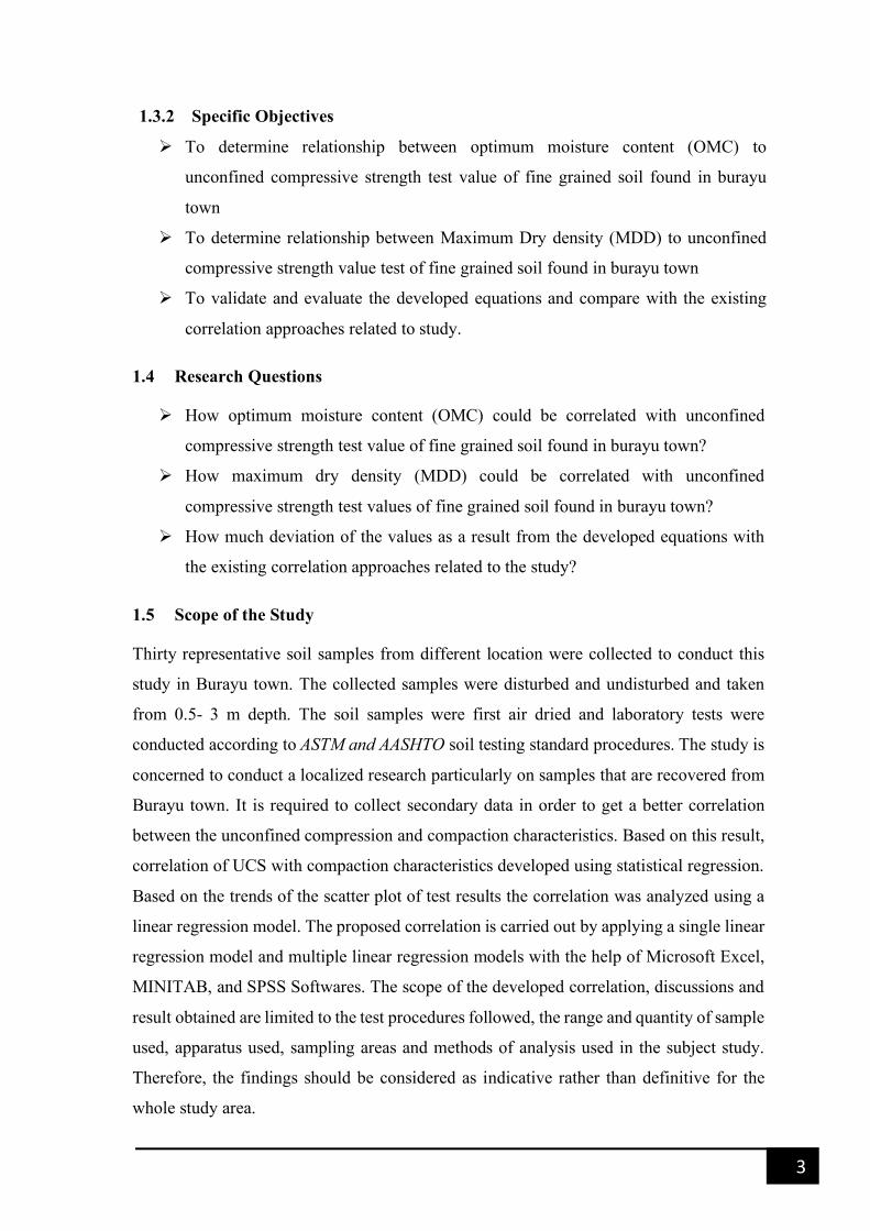
2.2.3 Predicting Undrained Shear Strength
Using the consistency of molded clay soil physical property, one may predict the undrained
shear strength of clay soils in the field simply by using one’s finger. Table 2.1 shows
general relationship of consistency and Unconfined Compression Strength (UCS) of clays
[8]
Table 2-1 General Relationship of Consistency and UCS of Clays [8]
Consistency qu(kN/m2) Remark
Very Soft 0-25 Squishes between finger when squeezed
Soft 25-50 Very easily deformed by squeezing
Medium Stiff (firm) 50-100 Thumb makes impression to deform
Stiff 100-200 Hard to deform by hand squeezing
Very Stiff 200-400 Very hard to deform by hand
Hard >400 Nearly impossible to deform by hand

7
2.3 compaction of soil
compaction means pressing the soil particle close to each other by mechanical means. It is
improving of the soil by increasing the dry density of a soil [5].
Compaction is required in many instances; examples include for the base layer of
pavements, for embankment fills, for retaining wall backfills, for fill around pipes, and for
landfills[12].
2.3.1 Factors Affecting Compaction
Besides moisture content, other important factors that affect compaction are soil type and
compaction effort (energy per unit volume)[13].The importance of each of these two factors
is described below
2.3.1.1 Effect of Soil Type
The soil type—that is, grain-size distribution, shape of the soil grains, specific gravity of
soil solids, and amount and type of clay minerals present—has a great influence on the
maximum dry unit weight and optimum moisture content. Note also that the bell-shaped
compaction curve is typical of most clayey soils. for sands, the dry unit weight has a general
tendency first to decrease as moisture content increases and then to increase to a maximum
value with further increase of moisture. The initial decrease of dry unit weight with increase
of moisture content can be attributed to the capillary tension effect. At lower moisture
contents, the capillary tension in the pore water inhibits the tendency of the soil particles to
move around and be compacted densely[13]
2.3.1.2 Effect of Compaction Effort
The compactive effort is defined as the amount of energy imparted to the soil. With a soil
of given moisture content, increasing the amount of compaction results in closer packing
of soil particles and increased dry unit weight.[9]
The compaction energy per unit volume used for the Proctor test
" = $%&'()*,-(.,/01)*.23)* 4∗67&'()*,-.23)*0 8∗9/):;<=,-<2'')* >∗6 <):;<=,-?*,1<2'')*8@,.&'),-',.? (.2.1)
8
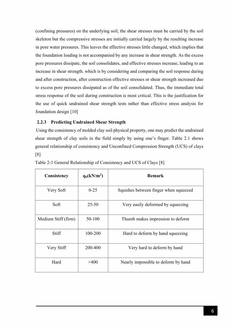
Figure 2-1 Effect of Compaction Effort in Compaction Curve [12]
As the compaction effort is increased, the maximum dry unit weight of compaction is
increased and the optimum moisture content is decreased to some extent [9]
Also, coarse-grained soils tend to reach optimum compaction at water contents lower than
fine-grained soils. However, coarse-grained soils tend to reach maximum dry densities that
are higher than those of fine-grained soils [12]
2.4 Review of Empirical Correlations
In Geotechnical engineering different correlations have been conducted. the study
presented by[4] studied Correlation Between Maximum Dry Density And Cohesion Of
Remoulded Nsukka Clays. The results were given by this research was A = 2.4267G?H +80.5G? − 743.86with a correlation coefficient of R= 0.679 for low plasticity clay (CL)
and A = 2.5058G?H + 89.195G? − 871.06with a correlation coefficient of R= 0.93 for
High plasticity clay (CH).
[14]tried to investigate fine grained soil to determine correlations between compaction
characteristics and Atterberg limits. The soils used were obtained from Addis Ababa. From
statistical analysis, he was correlate optimum moisture content and maximum dry density
with plastic limit and plasticity index. The results were given separately as OMC =

9
0.916 ∗ PL − 0.030 ∗ PI − 0.875 and MDD = −0.18 ∗ PL − 0.027 ∗ PI +21.182. the Functional Correlations between Compaction Characteristics, Un-drained
Shear Strength and Atterberg Limits presented by [15]. The results were given as XYA =0.233Z[ + 8 with a regression coefficient of R2=0.979 and G\ = −0.035Z[ + 18.498
with a regression coefficient of 0.976.
the Empirical correlation between undrained shear strength and pre-consolidation pressure
in Swedish soft clays showed by[16].The results were given as ]^_` = 0.15 + 0.16ab with
a regression coefficient of R2=0.979. this result showed that the undrained shear strength is
mainly depends on the stress history in a given soil.
the correlation of the undrained shear strength and plasticity index of tropical clays studied
by [17]. The results were given as cdefg = 2.342 − 2.175(Z[/100) a regression
coefficient of R2= – 0.882%. from the result the undrained shear strength (qu) value are
inversely proportional to the plasticity index of the clay soil. If the plasticity index increases
the undrained shear strength decreases.
according to the study conducted by [18] studied Developing Correlation between Dynamic
Cone Penetration Index (DCPI) and Unconfined Compression Strength (UCS) of the Soils
in Alem Gena Town. The results were given as kAl = −24.56 ∗ ln(oAZ[) + 223.05
with a regression coefficient of R2= 0.805% for black expansive soil. kAl = −58.59 ∗ln(oAZ[) + 308.04 with a regression coefficient of R2= 0.831%.
2.5 laboratory test
2.5.1 Natural Moisture Content
for many soils, the water content is one of the most important index properties used in
establishing the relationship between soil behavior and its index properties. The water
content of a soil is used in expressing the phase relationships of air, water, and solids in a
given volume of soil. In (cohesive) soils, the consistency of a given soil type depends on
its water content [19]
2.5.2 Specific Gravity
Specific gravity of soil is the ratio of weight of a given volume of soil particles in air at a
stated temperature to the weight of an equal volume of distilled water at a stated
temperature. The specific gravity of a soil is used to relate a weight of soil to its volume. It
also used to calculate phase relationships of soils [20]

10
2.5.3 Grain-size Distribution
Grain size analysis is an important parameter, to determine the percentage of different grain
sizes contained within a soil. It is required for classifying the soil as well as provides the
grain size distribution of the soil. Two methods are mostly used to determine grain size
distribution are Sieve analysis for coarse grained portion of the soil (size coarser than
0.075mm) and Hydrometer analysis for fine grained. Simple sieve analysis is used for
particles larger than 0.075mm while sedimentation analysis for particles smaller than
0.075mm. For soil sample that contains a measurable portion of their grains both coarser
and finer than 0.075mm size combined analysis is required. Portions (size finer than
0.075mm).
2.5.4 Atterberg Limits
Atterberg Limits are defined as water contents at certain limiting or critical ranges in soil
behavior. It also indicates the points at which the consistency of a fine-grained changes
from a liquid state to a plastic state (liquid limit), from a plastic state to a semisolid state
(plastic limit), and from a semisolid state to a solid state (shrinkage limit). They are used
in classification of fine-grained soils [12]
The sample of soil passing sieve No 40(0.425mm) is used to determine the Atterberg
Limits.
2.5.5 Classification of the Soils
Soil classification is the distribution of soils into different groups such that the soils in a
particular group have similar property. It is the type of labelling of soils with similar size.
As there is a wide variety of soils covering the earth, it is desirable to systemize or classify
the soils into broad groups of similar property [5]
there are various soil classification systems are existing in the world, Presently, two of
classification systems are frequently used by geotechnical and soil engineers. Both
systems take into account the particle-size distribution and Atterberg limits. They are the
American Association of State Highway and Transportation Officials (AASHTO)
classification system and the Unified Soil Classification System. The soils in this study
have been classified according to UCSC.
11
2.5.6 Unified Soil Classification System
This type of classification system is the most common for use in all types of engineering
problems including soils. This type of system classifies soils into two broad categories:
Ø Coarse-grained soils that are gravelly and sandy in nature with more than 50%
retained through the No.200 sieve. The group symbols start with a prefix of G or S.
G stands for gravel or gravelly soil, and S for sand or sandy soil.
Ø Fine-grained soils are with less than 50% retained through the No.200 sieve. The
group symbols start with prefixes of M, which stands for inorganic silt, C for
inorganic clay, or O for organic silts and clays. The symbol Pt is used for peat,
muck, and other highly organic soils [8]
2.5.7 Plasticity Chart
The plasticity chart is a plot of the plasticity index versus the liquid limit of a soil and it is
used for classifying fine-grained soils according to their plasticity. The A line is an
empirically chosen line that splits the chart between clays above the A line and silts below
the A line. The vertical line, corresponding to a liquid limit equal to 50%, separates high-
plasticity fine-grained soils(wL>50) from low-plasticity fine-grained soils (wL<50).To
classify a soil, the plasticity index and liquid. limit of that soil are plotted on the chart; the
region in which the point falls indicates what type of fine-grained soil it is or what kind of
fines are encountered in a coarse-grained soil. The plasticity chart is the basis for the
classification of fine-grained soils and of the fines fraction of coarse-grained soils [12]
2.5.8 Compaction Test
compaction means pressing the soil particle close to each other by mechanical means. It is
improving of the soil by increasing the dry density of a soil[5].
To determine the dry density of the soil, the wet unit weight of the soil is first determining
by using the following equation.
p/)= = qr@r (2.2)
Then, to determine the dry density of the soil by the following equation
γt = uvwxyz{ (2.3)
Compaction is the process of compressing the soil and reducing the air void by using
mechanical means. The purpose of compaction is increasing soil physical properties used
12
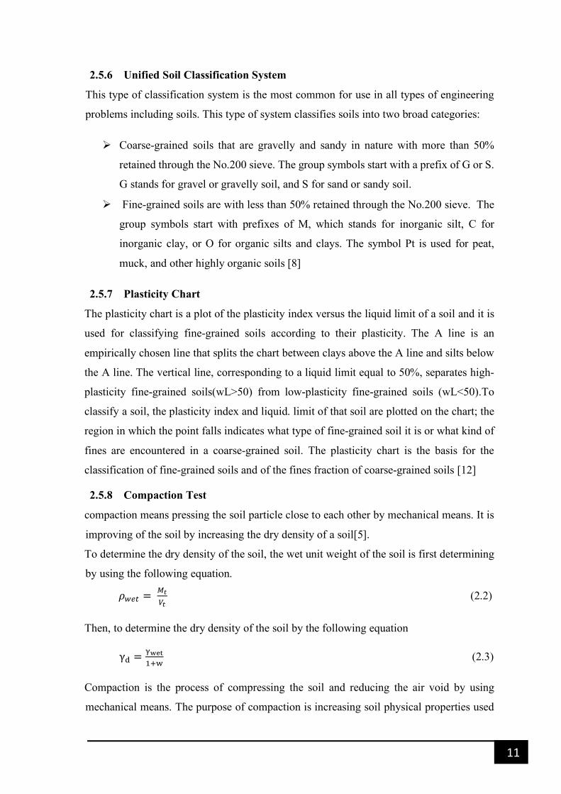
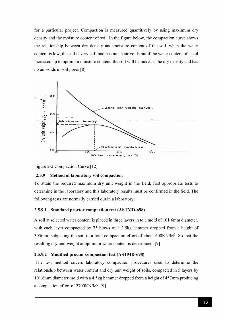
for a particular project. Compaction is measured quantitively by using maximum dry
density and the moisture content of soil. In the figure below, the compaction curve shows
the relationship between dry density and moisture content of the soil. when the water
content is low, the soil is very stiff and has much air voids but if the water content of a soil
increased up to optimum moisture content, the soil will be increase the dry density and has
no air voids in soil pores [8]
Figure 2-2 Compaction Curve [12]
2.5.9 Method of laboratory soil compaction
To attain the required maximum dry unit weight in the field, first appropriate tests to
determine in the laboratory and this laboratory results must be confirmed in the field. The
following tests are normally carried out in a laboratory.
2.5.9.1 Standard proctor compaction test (ASTMD-698)
A soil at selected water content is placed in three layers in to a mold of 101.6mm diameter.
with each layer compacted by 25 blows of a 2.5kg hammer dropped from a height of
305mm, subjecting the soil to a total compaction effort of about 600KN/M2. So that the
resulting dry unit weight at optimum water content is determined. [9]
2.5.9.2 Modified proctor compaction test (ASTMD-698)
The test method covers laboratory compaction procedures used to determine the
relationship between water content and dry unit weight of soils, compacted in 5 layers by
101.6mm diameter mold with a 4.5kg hammer dropped from a height of 457mm producing
a compaction effort of 2700KN/M2. [9]

13
2.5.10 Unconfined Compression Strength (UCS) Test
The most direct quantitative measure of consistency is the load per unit area at which
unconfined cylindrical samples of the soil fails in compression test. This quantity is known
as the unconfined compressive strength of the soil[12].
The unconfined compression test is a special case of a triaxial compression test in which
the tests are carried out only on saturated samples which can stand without any lateral
support. The test, is, therefore, applicable to cohesive soils only. The test Shear Strength
of Soil is an undrained test and is based on the assumption that there is no moisture loss
during the test[8].
In this test the sample is a cylinder with a diameter d and a height h equal to about 2 times
the diameter. The ratio h/d is about 2 to ensure that the oblique shear plane that typically
develops during failure can propagate through the entire sample without intersecting the
top or bottom platen. The sample remains unconfined during the test; therefore, the minor
principal stress σ3 is zero. A vertical load is applied to the sample by pushing upon the
bottom platen at a constant rate of displacement while holding the top platen in a fixed
position[12].
The vertical total stress σ is calculated by dividing the vertical load by the cross-sectional
area of the sample. Because it is assumed that there is no shear between the top of the
sample and the bottom of the top platen that stress is the major principal stress σ1. the
unconfined compression test gives both an undrained shear strength and a modulus of
deformation for fine-grained soils. Axial stress on the specimen is gradually increased until
the specimen fails. The sample fails either by shearing on an inclined plane (if the soil is
of brittle type) or by bulging. The vertical stress at any stage of loading is obtained by
dividing the total vertical load by the cross-sectional area. The cross-sectional area of the
sample increases with the increase in compression [8]
The cross-sectional area A at any stage of loading of the sample may be computed on the
basic assumption that the total volume of the sample remains the same. That is
|dℎd = |ℎ (2.4)
Where Ao, ho is equal to initial cross-sectional area and height of sample respectively.
And also, A, h is equal to cross-sectional area and height respectively at any stage of
loading.
If ∆h is the compression of the sample, the strain ε
ε = ∆ÄÄ (2.5)

14
since ∆h =ho-h, we may write Aoho= A (ho- ∆h) Therefore,
| = ÅÇÉÇ<ÇÑ∆É = ÅÇyÖ∆ÉÉÇ
= ÅÇyÖÜ (2.6)
The average vertical stress at any stage of loading may be written as
áy = àÅ = à(yÖÜ)
Å (2.7)
where P is the vertical load at the strain ε. Using the relationship given by Eq. (2.7) stress-
strain curves may be plotted. The peak value is taken as the unconfined compressive
strength qu,[9]
Figure 2-3 Mohr -Circle on Undrained Condition [8]
The unconfined compression test (UC) is a special case of the unconsolidated-undrained
(UU) triaxial compression test. The only difference between the UC test and UU test is that
a total confining pressure under which no drainage was permitted was applied in the latter
test. Because of the absence of any confining pressure in the UC test, a premature failure
through a weak zone may terminate an unconfined compression test [8]

15
CHAPTER -THREE
3 MATERIALS AND METHODS
In this Chapter laboratory analysis of collected samples and correlation and regression
methods were presented. Laboratory tests were conducted in Jimma University, geo-
technical Engineering Laboratory. Secondary data which was used to describe geological
condition of the study area as well as test result of unconfined compressive strength and
compaction test value was obtained from Google Map and some construction projects in
burayu town.
3.1 Description of the Study Area
The study was conducted in the western Oromia Burayu town. Burayu town is located in
the Oromia National, Regional State on the western fringe of Addis Ababa, along the Addis
Ababa-Ambo road; 15km away from the center of Addis Ababa measured from the Piazza.
Astronomically the town extends roughly from 9o02’ to 9o02'30" North latitudes and
38o03'30" to 38o41'30" East longitudes. According to census, the population of Burayu
town was 4,138 in 1984; 10,027 in 1994, 63,873 in 2007 and 100,200 in 2010 (estimated).
The Burayu town administration has estimated that the population of the town has grown
to more than 250,000 in 2018 [21].Location of the research area is shown in figure 3.1
below.
Figure 3-1 Location of the research area (Source: From Google Map)
16
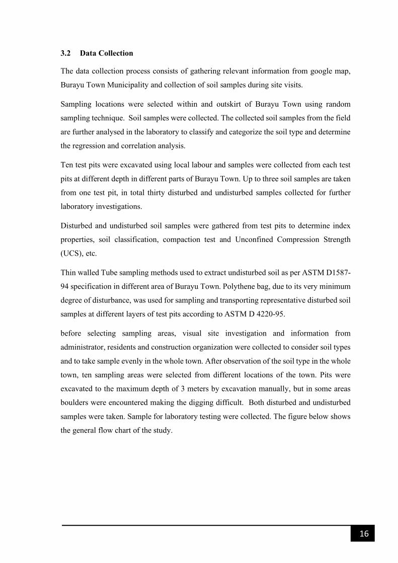
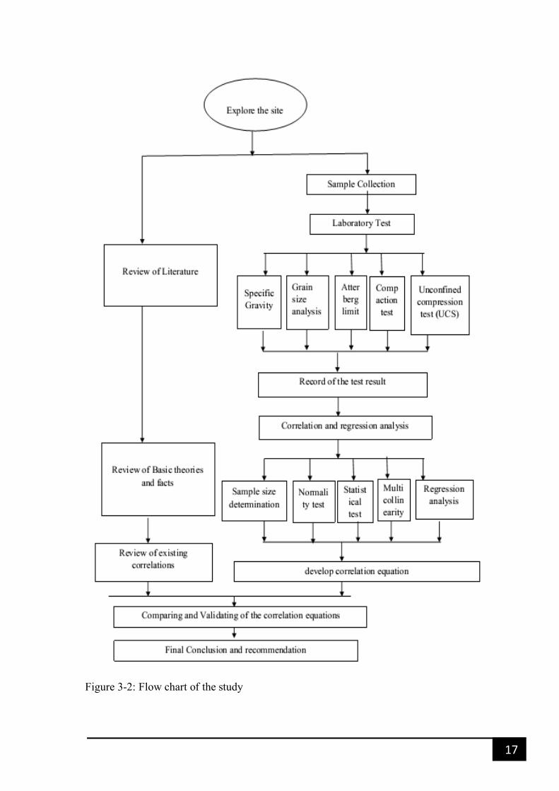
3.2 Data Collection
The data collection process consists of gathering relevant information from google map,
Burayu Town Municipality and collection of soil samples during site visits.
Sampling locations were selected within and outskirt of Burayu Town using random
sampling technique. Soil samples were collected. The collected soil samples from the field
are further analysed in the laboratory to classify and categorize the soil type and determine
the regression and correlation analysis.
Ten test pits were excavated using local labour and samples were collected from each test
pits at different depth in different parts of Burayu Town. Up to three soil samples are taken
from one test pit, in total thirty disturbed and undisturbed samples collected for further
laboratory investigations.
Disturbed and undisturbed soil samples were gathered from test pits to determine index
properties, soil classification, compaction test and Unconfined Compression Strength
(UCS), etc.
Thin walled Tube sampling methods used to extract undisturbed soil as per ASTM D1587-
94 specification in different area of Burayu Town. Polythene bag, due to its very minimum
degree of disturbance, was used for sampling and transporting representative disturbed soil
samples at different layers of test pits according to ASTM D 4220-95.
before selecting sampling areas, visual site investigation and information from
administrator, residents and construction organization were collected to consider soil types
and to take sample evenly in the whole town. After observation of the soil type in the whole
town, ten sampling areas were selected from different locations of the town. Pits were
excavated to the maximum depth of 3 meters by excavation manually, but in some areas
boulders were encountered making the digging difficult. Both disturbed and undisturbed
samples were taken. Sample for laboratory testing were collected. The figure below shows
the general flow chart of the study.
17
Figure 3-2: Flow chart of the study

18
The global coordinates of sampling location i.e. northing, easting and elevations are shown
in Table 3.1
Table 3-1 Global coordinates of sampling areas
3.3 Laboratory Analysis
The engineering properties soils are classified and identified based on index properties and
other tests. Some of this properties of soil are; Natural moisture content, Specific gravity,
consistency limits, Grain size analysis, compaction test and unconfined compressive
strength. The entire laboratory tests were performed in Jimma institute of Technology
geotechnical engineering Laboratory using the following standard testing procedures,
(Table 3-2).
Table 3-2 Summary of laboratory testing procedure standards
3.4 Steps for correlation and Regression Analysis
3.4.1 Sample size determination
In most studies the sample size is determined effectively by two factors: (1) the nature of
data analysis proposed and (2) estimated response rate. [22]
Test Pit Location Northing Easting Elevation (m)
TP-1 Leku Keta 9.05716 38.68164 2512
TP-2 Burayu Keta 9.07458 38.67604 2585
TP-3 Leku Keta 2 9.07283 38.68488 2586
TP-4 Gefersa Burayu 9.07001 38.66317 2616
TP-5 Gefersa Nono 2 9.06383 38.61156 2619
TP-6 Gefersa guji 2 9.08048 38.62752 2640
TP-7 Gefersa Nono 9.07306 38.61956 2615
TP-8 Melka gefersa 2 9.05467 38.63716 2605
TP-9 Gefersa guji 9.07831 38.63816 2610
TP-10 Melka gefersa 9.05647 38.65123 2600
Test Description Standard Testing Procedure
Grain Size Distribution Analysis ASTM D 1140-97 and D 422-98
Natural Moisture Content ASTM D 2216-98a
Atterberg Limits ASTM D 4318-98
Specific Gravity ASTM D 854-98
Compaction test ASTM D698
Unconfined Compressive Strength ASTM D2166-98a

19
Margin of error is the statistics, expressing the amount of random variable sampling error
in the survey analysis. The higher margin of error the lessor confidence interval. It is ½ half
the width of confidence interval. A larger sample size produces the smaller the margin
error. The standard deviation of population found from previous researches and literatures.
confidence interval is used to indicate the reliability of an estimate. The calculation is
worked firstly by selection of the desired confidence level. To determine the sample size,
if the standard deviation of the population known, the following formula is used
â = =ä/ãã ∗_ãåã (3.1)
If the population is unknown, the following formula is used to determine sample size for
sample proportion
â = =ä/ãã ∗1(yÖ1é )åã (3.2)
σ2 =standard deviation
E2= Margin of error rate
è =percentage picking a choice or population proportion response
tα/2 = 1.962 at 95% of confidence level
N=sample size
3.4.2 Normality Test
Normality test is used to check whether the data fulfill assumption of normally distributed
or not. It also helps to choose parametric or Non-parametric statistical tests. There are many
tests to check whether the data is normally distributed or not. these tests basically classified
as graphical and non-graphical tests for assessing univariate normality. One of the most
popular graphical tests is the normal probability plot, where the observations are arranged
in increasing order of magnitude and then plotted against expected normal distribution
values. The plot should resemble a straight line if normality is tenable. [23]
One could also examine the histogram of the variable in each group. This gives some
indication of whether normality might be violated. However, with small or moderate
sample sizes, it is difficult to tell whether the non-normality is real or apparent, because of
considerable sampling error. Therefore, most researcher prefer a non-graphical test. Among
the non-graphical tests are the Kolmogorov-Smirnov, the Shapiro-Wilk test, and the use of
skewness and kurtosis coefficients. the Kolmogorov-Smirnov test was shown not to be as
20
powerful as the Shapiro-Wilk test. The combination of skewness and kurtosis coefficients
and the Shapiro-Wilk test were the most powerful in detecting departures from normality.
The procedure also yields the skewness and kurtosis coefficients, along with their standard
errors. All of this information is useful in determining whether there is a significant
departure from normality, and whether skewness or kurtosis is primarily responsible.[24]
Data showing a moderate departure from normality can usually be used in parametric
procedures without loss of integrity. Also, for comparing means and sample size (for each
group) is “large” (say,>= 30), we can invoke the central limit theorem (CLT) to justify
using parametric procedures even when the data are not normally distributed. Briefly, the
CLT states that sample means are approximately normal for sufficiently large sample sizes
even when the original populations are non-normal.[25]
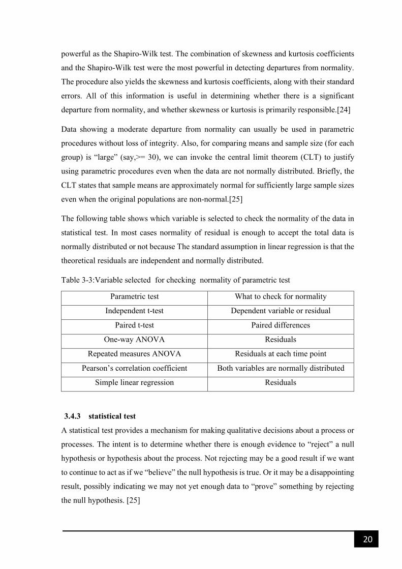
The following table shows which variable is selected to check the normality of the data in
statistical test. In most cases normality of residual is enough to accept the total data is
normally distributed or not because The standard assumption in linear regression is that the
theoretical residuals are independent and normally distributed.
Table 3-3:Variable selected for checking normality of parametric test
Parametric test What to check for normality
Independent t-test Dependent variable or residual
Paired t-test Paired differences
One-way ANOVA Residuals
Repeated measures ANOVA Residuals at each time point
Pearson’s correlation coefficient Both variables are normally distributed
Simple linear regression Residuals
3.4.3 statistical test
A statistical test provides a mechanism for making qualitative decisions about a process or
processes. The intent is to determine whether there is enough evidence to “reject” a null
hypothesis or hypothesis about the process. Not rejecting may be a good result if we want
to continue to act as if we “believe” the null hypothesis is true. Or it may be a disappointing
result, possibly indicating we may not yet enough data to “prove” something by rejecting
the null hypothesis. [25]

21
3.4.3.1 Parametric and non-parametric statistical tests
Parametric tests are more strong and for the most part require less data to make a stronger
conclusion than nonparametric tests. However, to use a parametric test, the data must be
fulfilling normality test and also the data need to be continuous and Interval or ratio level
of measurement. If the data do not meet the criteria for a parametric, before we conduct
non –parametric test it must be checked by data transformation method or normalization
method. It is not possible; it must be analyzed with a nonparametric test. If a
nonparametric test is required, more data will be needed to make the same conclusion.
[23]
Non-parametric tests make no assumptions about the distribution of the data.
Nonparametric techniques are usually based on ranks or signs rather than the actual data
and are usually less powerful than parametric tests.[24]
Commonly used parametric and nonparametric tests are described below by the following
table.
Table 3-4: Methods for determining parameter and non-parametric statistical test
Parametric Test Non-parametric test
Independent – samples T-test Mann-Whitney Test
Paired samples T-test Wilcoxon Signed-Rank Test
One-Way ANOVA
Kruskal-Wallis and Friedman’s ANOVA One-Way repeated measures of ANOVA
3.4.3.2 Parametric Tests
3.4.3.2.1 t-Test
The Student t-test is probably the most widely used parametric test. A single sample t-test
is used to determine whether the mean of a sample is different from a known average. A
pair-sample t-test is used to establish whether a difference occurs between the means of
two similar data sets. The independent t-test, also called the two sample t-test, independent-
samples t-test or student's t-test, is a statistical test that determines whether there is a
statistically significant difference between the means in two independent variables.[26] The
t-test uses the mean, standard deviation, and number of samples to calculate the test
statistic. In a data set with a large number of samples, the critical value for the t-test is 1.96
for an alpha of 0.05, obtained from a t-test table.

22
3.4.3.2.2 The z-Test
The next test, which is very similar to the t-test, is the z-test. However, with the z-test,
the variance of the standard population, rather than the standard deviation of the study
groups, is used to obtain the z-test statistic. Using the z-chart, like the t-table, we see what
percentage of the standard population is outside the mean of the sample population. If,
like the t-test, greater than 95% of the standard population is on one side of the mean, the
p-value is less than 0.05 and statistical significance is achieved. As some assumption of
sample size exists in the calculation of the z-test, it should not be used if sample size is
less than 30. If both the n and the standard deviation of both groups are known, a pair
sample t-test is best.[26]
3.4.3.2.3 ANOVA Test
Analysis of variance (ANOVA) is a test used to determine if one or more of the means of
several groups is different from others. it incorporates means and variances to determine
the test statistic. The test statistic is then used to determine whether groups of data are the
same or different. When hypothesis testing is being performed with ANOVA, the null
hypothesis is stated such that all groups are the same. The test statistic for ANOVA is
called the F-ratio.[25]
3.4.4 Transformation of data(normalization)
Data transformation can correct deviation from normality and uneven
variance(heteroscedasticity). If The data is not normally distributed, parametric test is not
allowed to use in testing the differences between means of variable. To use the parametric
test, we need first of all to normalize the data by using the transformation function
recommended in statistics. The logarithm, square root and the reciprocal transformation is
commonly used method. After transform the data, histogram, Q-Q plots and Box plot is
plot to verify if the log data are approximately normally distributed. If the transformation
of data is not fulfilling assumption of normally distributed, we use nonparametric test.[25]
3.4.5 Nonparametric Tests
3.4.5.1.1 Mann-Whitney U Test
This test uses rank just as the previous test did. It is analogous to the t-test for continuous
variable but can be used for ordinal data. This test compares two independent populations
to determine whether they are different. The sample values from both sets of data are
ranked together. Once the two test statistics are calculated, the smaller one is used to

23
determine significance. Unlike other tests, the null hypothesis is rejected if the test
statistic is less than the critical value. The U-value is widely available for this test.[26]
3.4.5.1.2 Kruskal-Wallis Test
The Kruskal-Wallis test uses ranks of ordinal data to perform an analysis of variance to
determine whether multiple groups are similar to each other. This test ranks all data from
the groups into one rank order and individually sums the different ranks from the
individual groups. These values are then placed into a larger formula that computes an
H-value for the test statistic. The degrees of freedom used to find the critical value is the
number of groups minus one. [26]
3.4.6 Multicollinearity (interdependency check)
Multicollinearity refers to the situation in which two or more independent variables in a
multiple linear regression model are highly correlated. Multicollinearity poses a real
problem for the researcher it increases the variances of the regression coefficients. The
greater these variances, the more unstable the prediction equation will be.[27] The
following are two methods for diagnosing multicollinearity:
Ø Examine the simple correlations among the predictors from the correlation matrix.
These should be observed, and are easy to understand, but the researcher needs to be warned
that they do not always indicate the extent of multicollinearity.
Ø Variance inflation factor is the measure that can be used to quantify
multicollinearity. The quantity 1/ (1 - R2j) is called the jth variance inflation factor, where
R2j is the squared multiple correlation for predicting the jth predictor from all other
predictors. the reciprocal of the above formula is called tolerances. The variance inflation
factor for a predictor indicates whether there is a strong linear association between it and
all the remaining predictors. It is distinctly possible for a predictor to have only moderate
or relatively weak associations with the other predictors in terms of simple correlations.
If the value for a variance inflation factor VIF exceeds 10, there is multicollinearity
between the predictors. [28]

24
3.4.7 Correlation and regression methods
Various method used for determining the adequacy of the different regression models
obtained. A commonly used methods are listed below.
3.4.7.1 The Standard Error Statistics
The standard error of a statistic gives some idea about the precision of an estimate.
Estimated standard errors are computed based on sample estimates, as population values
are not obtainable using sample surveys [29].The estimated standard error of a variable
with mean and standard deviation of SD is given by
á = ]ê√% (3.4)
Where: σ=estimated standard error of a sample.
n=sample size
During modelling, a variable that shows the least standard error of estimates is the one to
be relatively chosen.
3.4.7.2 Residual Analysis
Residual analysis is Any technique that uses the residuals, usually to investigate the
adequacy of the model that was used to generate the residuals. a residual is the difference
between the observed value of the response and the corresponding predicted value
obtained from the regression model. Analysis of the residuals is frequently helpful in
checking the assumption that the errors are approximately normally distributed with
constant variance, and in determining whether additional terms in the model would be
useful. Residuals that are far outside from the interval from normal probability plots may
indicate the presence of an outlier, that is, an observation that is not typical of the rest of
the data. Various rules have been proposed for discarding outliers. However, outliers
sometimes provide important information about unusual circumstances of interest to
experimenters. If the residual of an observation is larger than 3 times of the standard
deviation (or standardized residual is larger than 3) then the observation may be considered
as an outlier [26]
3.4.7.3 Coefficient of Determination(R2)
A quantity used in regression models to measure the proportion of total variability in the
response accounted for the model. Computationally, large values of R2(near unity) are
considered good. However, it is possible to have large values of R2 and find that the model

25
is unsatisfactory. R2 is also called the coefficient of determination (or the coefficient of
multiple determination in multiple regression) [29]
The value of R2 is always between 0 and 1, because R is between -1 and +1, whereby a
negative value of R indicates inversely relationship and positive value implies direct
relationship and it is given by the equation[30].
íH = ]]ì]]î = 1− ]]å
]]î (3.5 )
Where:
llî =ï(ñ − ñó)H%
:òy
llå =ï(ñ: − ñó:)H%
:òy
And llì = llî − llå = regression sum of squares
ll" error sum of squares
llô=total sum of squares
öõ=ith value of the response variable
öó:=ith value of the fitted response variable.
ñó=average value of the response variable
3.4.7.4 Adjusted R2
Another useful criterion used to check the adequacy of a regression model is using a
modified R2 that accounts the usefulness of a variable in a model. It essentially penalizes
the analyst for adding terms to the model[29].
This statistic is called the adjusted R2 defined as:
íàH = 1 − %Öy%Ö11 (1 − íH) (3.6)
Where: =number of regressors in the regression model
=Sample size
=adjusted coefficient of determination.
Maximizing the value of R2 by adding variables is inappropriate unless variables are added
to the equation for sound theoretical reason. At an extreme, when n-1 variables are added
to a regression equation, R2 will be 1, but this result is meaningless. Adjusted R2 is used as

26
a conservative reduction to R2 to penalize for adding variables and is required when the
number of independent variables is high relative to the number of cases or when comparing
models with different numbers of independents .During regression analysis, a regression
model with higher value of adjusted is usually accepted[26]
3.4.7.5 Correlation Coefficients
Correlation coefficients measures the strength of linear association between two
measurement variables.
3.4.7.5.1 Pearson’s correlation coefficient
Pearson’s correlation coefficient or simply correlation coefficient, R, measures the strength
of linear association between two measurement variables. It is calculated as: [30]
í = ú,ù(û,3)0?(û)∗0?(3) (3.7)
Where:
†d°(¢, ñ) = ∑ (¢: − ¢)(ñ: − ñó)%:ò§ =covariance of x and y variable
•\(¢) = ¶∑ (¢: − ¢)%:ò§ =standard deviation of variable x
•\(ñ) = ¶∑ (ñ: − ñó)%:ò§ =standard deviation of variable y
The value of R ranges from -1 to +1. A value of the correlation coefficient closes to +1
indicates a strong positive linear relationship (i.e. one variable increases with the other) A
value close to -1 indicates a strong negative linear relationship (i.e. one variable decreases
as the other increases). A value close to 0 indicates no linear relationship; however, there
could be a nonlinear relationship between the variables[26]. The following key points
shows Assumptions used for conducting Pearson correlation.
Ø The two variables should be measured at the interval or ratio level
Ø There needs to be a linear relationship between the two variables
Ø There should be no significant outliers
Ø The variables should be approximately normally distributed
3.4.7.5.2 Spearman’s correlation coefficient
Is a nonparametric measure of the strength and direction of association that exists between
two variables measured on at least an ordinal scale. It is used for when the assumption
necessary for conducting the Pearson’s correlation is failed.
3.4.7.6 Hypothesis Testing of Regression
several problems in engineering require that we decide whether to accept or reject a
statement about some parameter. The statement is called a hypothesis, and the decision-

27
making procedure about the hypothesis is called hypothesis testing. This is one of the most
useful aspects of statistical inference, since many types of decision-making problems, tests,
or experiments in the engineering world can be formulated as hypothesis-testing problems
[7]
The t-test is one of the methods used to accept or reject a given hypothesis. The t- value is
simply calculated as
ßù2.&) = ®]å = ú,)--:ú:)%=,-2ù2*:2(.):%=<)*);*)00:,%)©&2=:,%
0=2%?2*?)**,*,-=<))0=:'2=)?ú,)--:ú:)%= (3.8)
Suppose we want to test the validity of a hypothesis; the hypothesis can be formulated as
follows:
™ ,: ≠ = Æy: ≠ ≠ Æ (3.9)
For an arbitrary population value of “a”, here “Ho “and “H1” are the null hypothesis and
alternative hypothesis, respectively. Let α denote the probability of rejecting a true
hypothesis (level of significance of the test), then the tabulated t-value (t-tab) that is used
to test the importance of a variable in the model is obtained by reading from the t-table with
α/2 as column an “n” as row, and α as row and “n-1” as column for two and one-sided
hypothesis, respectively. Here “n-1” denotes the degree of freedom[7].
By continuing in such fashion, it will be decided on the importance of each regression
variable in the model. If t-cal exceeds t-tab, then “Ho” is accepted; otherwise, the null
hypothesis is accepted. If “a=0”, for instance, accepting Ho means the particular variable
has no importance in explaining [7].
Nowadays, commercial statistical software can provide p-values. Hence, we may not need
tables for our particular decision. The P-value is the smallest level of significance at which
a variable is significant. If p- value is smaller than α, the particular variable is important in
explaining the variation of the response in the model. If Zo is the computed value of the
test statistics, then the p- value is 2(1-(Zo)) for two-tailed test. Here, (Zo) is the standard
normal cumulative distribution at Zo[26].
The p-value for each term tests the null hypothesis that the coefficient is equal to zero (no
effect). A low p-value (< 0.05) indicates that you can reject the null hypothesis. In other
words, a predictor that has a low p-value is likely to be a meaningful addition to your model
because changes in the predictor's value are related to changes in the response variable.
Conversely, a larger (insignificant) p-value suggests that changes in the predictor are not
associated with changes in the response [7]
28
CHAPTER –FOUR
4 RESULT AND DISCUSSIONS
4.1 Laboratory test result
The following laboratory result shows the primary data of the soil conducted on the study
area.
4.1.1 Grain-size Distribution
The result of the sieve and hydrometer analysis is shown in the following table and Figure
below.
Table 4-1 Grain Size analysis result
Test
pit Depth
Percent Amount Of Particle Size
%
finer
than
0.075
AASHTO system USCS system
Gravel Sand Silt Clay Gravel Sand Silt Clay
TP-
1
0.6 0.26 2.22 27.62 69.90 0.0 2.5 27.6 69.9 97.52
1.4 0.24 1.96 45.53 52.27 0.04 2.16 45.53 52.27 97.80
2.5 0.32 1.83 45.66 52.19 0.06 2.09 45.66 52.19 97.85
TP-
2
0.5 0.77 2.24 39.56 57.43 0.33 2.68 39.56 57.43 96.99
1.5 1.22 2.47 43.05 53.25 0.56 3.14 43.05 53.25 96.30
2.7 2.48 3.88 35.07 58.57 1.00 5.36 35.07 58.57 93.64
TP-
3
0.7 2.56 4.50 39.72 53.21 1.74 5.32 39.72 53.21 92.94
1.35 3.44 7.68 36.18 52.70 2.20 8.92 36.18 52.70 88.88
2.6 4.28 7.68 35.84 52.20 2.64 9.32 35.84 52.20 88.04
TP-
4
0.6 4.34 8.41 33.81 53.44 1.88 10.87 33.81 53.44 87.25
1.5 5.38 9.70 29.09 55.83 2.50 12.59 29.09 55.83 84.91
2.7 5.6 10.8 28.8 54.9 2.3 14.0 28.8 54.9 83.64
TP-
5
0.5 6.14 12.49 26.55 54.81 2.68 15.95 26.55 54.81 81.37
1.4 6.08 13.28 23.80 56.85 2.83 16.53 23.80 56.85 80.64
2.6 2.07 5.41 35.97 56.55 1.41 6.07 35.97 56.55 92.52
TP-
6
0.5 2.44 6.61 34.83 56.12 1.60 7.45 34.83 56.12 90.95
1.7 1.66 4.95 35.16 58.24 1.21 5.40 35.16 58.24 93.40
2.6 1.64 4.43 37.37 56.56 0.98 5.08 37.37 56.56 93.93
TP-
7
0.5 2.04 4.34 28.31 65.31 1.18 5.20 28.31 65.31 93.62
1.8 2.06 4.55 36.00 57.39 1.01 5.60 36.00 57.39 93.39
2.9 1.68 5.13 36.10 57.08 0.81 6.01 36.10 57.08 93.18
0.6 1.29 4.92 38.45 55.34 0.60 5.61 38.45 55.34 93.79

29
TP-
8
1.7 1.94 5.38 34.22 58.46 1.01 6.30 34.22 58.46 92.68
2.7 1.95 4.37 27.68 66.00 0.81 5.51 27.68 66.00 93.68
TP-
9
0.54 1.10 3.34 28.00 67.56 0.44 4.00 28.00 67.56 95.56
1.6 1.73 2.96 41.04 54.28 0.66 4.02 41.04 54.28 95.32
2.6 1.65 3.30 34.48 60.57 0.78 4.17 34.48 60.57 95.05
TP-
10
0.6 0.85 3.10 35.58 60.47 0.21 3.74 35.58 60.47 96.05
1.7 1.30 3.83 36.80 58.07 0.46 4.68 36.80 58.07 94.87
2.8 1.65 4.69 31.20 62.47 0.60 5.73 31.20 62.47 93.67
Figure 4-1 Grain size distribution curve for TP-1 to TP-5
Figure 4-2 Grain size distribution curve for TP-6 to TP-10
0
20
40
60
80
100
120
0.0010.010.1110100
Per
cen
tage
fin
er (
%)
Grain Size (mm)
Grain size Boundary According to ASTMTP-1-1
T-P-1-2
T-P-1-3
T-P-2-1
T-P-2-2
T-P-2-3
T-P-3-1
T-P-3-2
T-P-3-3
T-P-4-1
T-P-4-2
T-P-4-3
T-P-5-1
T-P-5-2
T-P-5-3
0.075 mm4.75 mm75 mmSiltSandGravel Clay
0.002 mm
0
20
40
60
80
100
120
0.0010.010.1110100Per
cen
tage
fin
er (
%)
Grain Size (mm)
Grain size Boundary According to ASTM T-P-6-1
T-P-6-2
T-P-6-3
T-P-7-1
T-P-7-2
T-P-7-3
T-P-8-1
T-P-8-2
T-P-8-3
T-P-9-1
T-P-9-2
T-P-9-3
T-P-10-1
T-P-10-2
T-P-10-3
0.075 mm4.75 mm75
mm
SiltSandGravel Cla0.002 mm
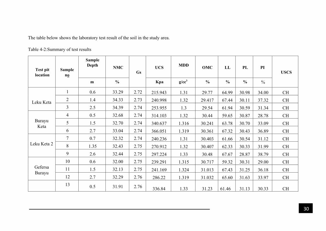
30
The table below shows the laboratory test result of the soil in the study area.
Table 4-2:Summary of test results
Test pit
location
Sample
no
Sample
Depth NMC
Gs UCS
MDD OMC LL PL PI
USCS
m % Kpa g/cc3 % % % %
Leku Keta
1 0.6 33.29 2.72 215.943 1.31 29.77 64.99 30.98 34.00 CH
2 1.4 34.33 2.73 240.998 1.32 29.417 67.44 30.11 37.32 CH
3 2.5 34.39 2.74 253.955 1.3 29.54 61.94 30.59 31.34 CH
Burayu
Keta
4 0.5 32.68 2.74 314.103 1.32 30.44 59.65 30.87 28.78 CH
5 1.5 32.70 2.74 340.637 1.316 30.241 63.78 30.70 33.09 CH
6 2.7 33.04 2.74 366.051 1.319 30.361 67.32 30.43 36.89 CH
Leku Keta 2
7 0.7 32.32 2.74 240.236 1.31 30.403 61.66 30.54 31.12 CH
8 1.35 32.43 2.75 270.912 1.32 30.407 62.33 30.33 31.99 CH
9 2.6 32.44 2.75 297.224 1.33 30.48 67.67 28.87 38.79 CH
Gefersa
Burayu
10 0.6 32.00 2.75 239.291 1.315 30.717 59.32 30.31 29.00 CH
11 1.5 32.13 2.75 241.169 1.324 31.013 67.43 31.25 36.18 CH
12 2.7 32.29 2.76 286.22 1.319 31.032 65.60 31.63 33.97 CH
13 0.5 31.91 2.76 336.84 1.33 31.23 61.46 31.13 30.33 CH

31
Gefersa
Nono 2
14 1.4 31.94 2.76 327.745 1.302 32.42 60.67 30.59 30.09 CH
15 2.6 31.99 2.76 355.946 1.333 32.21 61.52 30.65 30.86 CH
Gefersa guji
2
16 0.5 31.81 2.76 335.023 1.32 31.317 65.57 31.20 34.37 CH
17 1.7 31.84 2.77 341.724 1.339 32.373 67.88 31.39 36.49 CH
18 2.6 31.84 2.77 389.993 1.342 32.441 67.32 32.65 34.67 CH
Gefersa
Nono
19 0.5 31.69 2.77 344.344 1.33 31.864 61.54 30.99 30.55 CH
20 1.8 31.77 2.78 346.119 1.344 30.73 69.37 32.98 36.39 CH
21 2.9 31.80 2.78 349.74 1.351 31.307 67.24 32.09 35.15 CH
Melka
gefersa 2
22 0.6 31.350 2.79 505.929 1.334 34.164 67.45 32.15 35.31 CH
23 1.7 31.423 2.79 516.787 1.354 33.541 70.36 33.19 37.18 CH
24 2.7 31.497 2.79 503.365 1.362 34.362 70.04 32.69 37.36 CH
Gefersa guji
25 0.54 31.28 2.80 432.729 1.367 32.54 68.96 32.68 36.28 CH
26 1.6 31.28 2.80 433.398 1.332 32.745 70.16 32.91 37.25 CH
27 2.6 31.33 2.80 496.635 1.344 33.343 68.41 32.04 36.37 CH
Melka
gefersa
28 0.6 30.98 2.80 429.519 1.35 32.703 70.19 33.12 37.07 CH
29 1.7 31.19 2.80 434.613 1.363 33.4 71.34 33.08 38.26 CH
30 2.8 31.20 2.81 483.557 1.371 32.992 69.47 33.09 36.38 CH

32
The following table shows secondary data of Unconfined compressive test and compaction test in
Burayu town.
Table 4-3 Secondary Data of UCS and Compaction Characteristics Value
no UCS(Kpa) MDD(g/cc3) Omc(%
1 218.5398 1.313 29.818
2 243.4143 1.323 29.465
3 256.9529 1.313 29.588
4 317.4043 1.323 30.488
5 344.4163 1.332 31.333
6 369.5853 1.335 32.268
7 241.7374 1.313 30.965
8 271.4163 1.323 30.018
9 299.5853 1.333 30.768
10 240.4874 1.318 29.538
11 242.5332 1.317 30.066
12 287.5432 1.322 30.179
13 339.5452 1.333 31.278
14 330.4551 1.315 32.468
15 358.6683 1.336 32.258
16 339.5031 1.323 31.365
17 334.8885 1.326 32.421
18 382.9476 1.339 32.489
19 407.6002 1.333 31.912
20 341.6833 1.323 30.778

33
4.1.2 Discussion on the laboratory test result
Ø The specific gravity of the soil from the study area ranges from 2.72-2.81 this shows the
soil is clay soil
Ø The results of grain size analysis for all test pits, the percentage of soil passing sieve no.200
is more than 80%. This means the soil is mainly fine grained soils. The hydrometer analysis
indicate that the soil of the study area is clay nature.
Ø Based on the USCS soil classification, the soil in the study area is categorized as CH
(highly plastic clay soil).
4.2 Correlation and regression result
4.2.1 Sample size result
! =#$/&& ∗ (&
)&
tα/2 =1.96 for 95% confidence interval
σ2 = Standard deviation=0.14 and 0.18
E= 0.05 for 95% confidence interval
For primary data
! =(+.-.)0∗1.+20
1.130= 30
For combined (primary and secondary data)
! =(+.-.)0∗1.+40
1.130= 50
4.2.2 Discussion on sample size result
The sample size result for primary and combined data was 30 and 50. Those result was depending
on the predicted standard deviation, margin of error and t-test value. According to [22] if ten or
above tests are made, the variation of their sample average from population would have a standard
deviation of 10–16%. Based the above stated reason the predicted standard deviation was 14 and
18% for sample size 30 and 50. The margin of error is dependent on the level of confidence. The
95% percent of level of confidence gives 5% of error from the population mean.
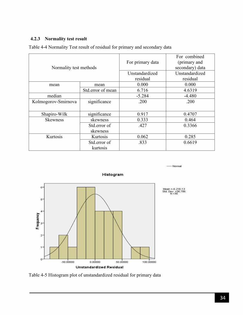
34
4.2.3 Normality test result
Table 4-4 Normality Test result of residual for primary and secondary data
Normality test methods
For primary data
For combined
(primary and
secondary) data
Unstandardized
residual
Unstandardized
residual
mean mean 0.000 0.000
Std.error of mean 6.716 4.6319
median -5.284 -4.480
Kolmogorov-Smirnova significance .200 .200
Shapiro-Wilk significance 0.917 0.4707
Skewness skewness 0.333 0.464
Std.error of
skewness
.427 0.3366
Kurtosis Kurtosis 0.062 0.285
Std.error of
kurtosis
.833 0.6619
Table 4-5 Histogram plot of unstandardized residual for primary data

35
Table 4-6 QQ plot of unstandardized residual for primary data
Table 4-7 Histogram plot of unstandardized residual for combined data
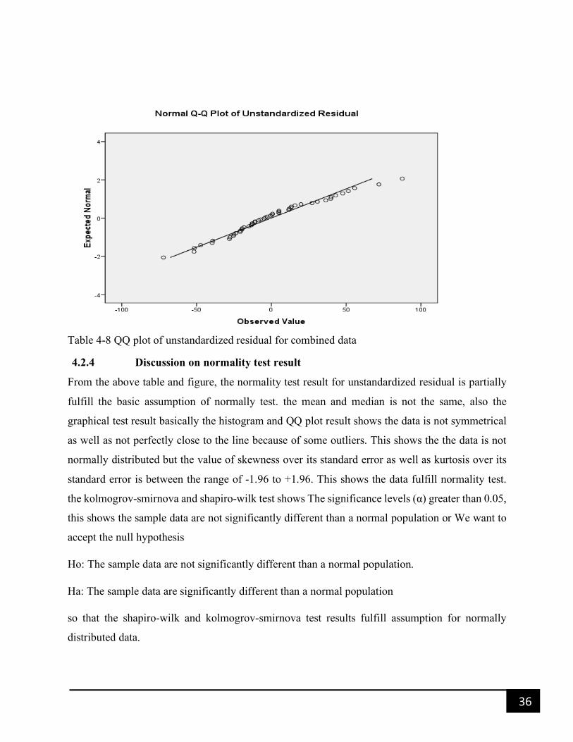
36
Table 4-8 QQ plot of unstandardized residual for combined data
4.2.4 Discussion on normality test result
From the above table and figure, the normality test result for unstandardized residual is partially
fulfill the basic assumption of normally test. the mean and median is not the same, also the
graphical test result basically the histogram and QQ plot result shows the data is not symmetrical
as well as not perfectly close to the line because of some outliers. This shows the the data is not
normally distributed but the value of skewness over its standard error as well as kurtosis over its
standard error is between the range of -1.96 to +1.96. This shows the data fulfill normality test.
the kolmogrov-smirnova and shapiro-wilk test shows The significance levels (α) greater than 0.05,
this shows the sample data are not significantly different than a normal population or We want to
accept the null hypothesis
Ho: The sample data are not significantly different than a normal population.
Ha: The sample data are significantly different than a normal population
so that the shapiro-wilk and kolmogrov-smirnova test results fulfill assumption for normally
distributed data.
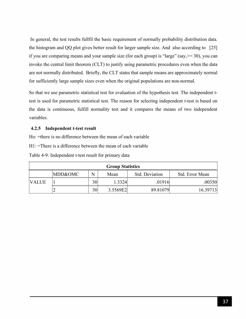
37
In general, the test results fullfil the basic requirement of normally probability distribution data.
the histogram and QQ plot gives better result for larger sample size. And also according to [25]
if you are comparing means and your sample size (for each group) is “large” (say,>= 30), you can
invoke the central limit theorem (CLT) to justify using parametric procedures even when the data
are not normally distributed. Briefly, the CLT states that sample means are approximately normal
for sufficiently large sample sizes even when the original populations are non-normal.
So that we use parametric statistical test for evaluation of the hypothesis test. The independent t-
test is used for parametric statistical test. The reason for selecting independent t-test is based on
the data is continuous, fulfill normality test and it compares the means of two independent
variables.
4.2.5 Independent t-test result
Ho: =there is no difference between the mean of each variable
H1: =There is a difference between the mean of each variable
Table 4-9: Independent t-test result for primary data
Group Statistics
MDD&OMC N Mean Std. Deviation Std. Error Mean
VALUE 1 30 1.3324 .01916 .00350
2 30 3.5569E2 89.81079 16.39713
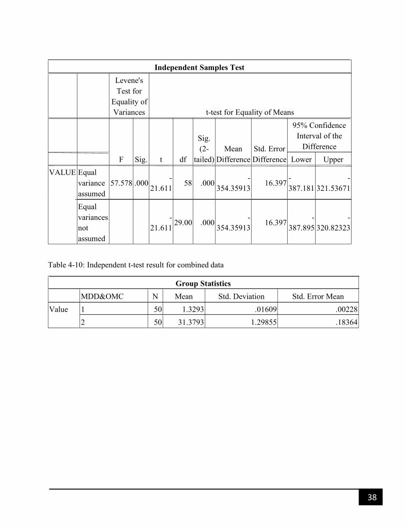
38
Independent Samples Test
Levene's
Test for
Equality of
Variances t-test for Equality of Means
F Sig. t df
Sig.
(2-
tailed)
Mean
Difference
Std. Error
Difference
95% Confidence
Interval of the
Difference
Lower Upper
VALUE Equal
variance
assumed
57.578 .000 -
21.611 58 .000
-
354.35913 16.397
-
387.181
-
321.53671
Equal
variances
not
assumed
-
21.611 29.00 .000
-
354.35913 16.397
-
387.895
-
320.82323
Table 4-10: Independent t-test result for combined data
Group Statistics
MDD&OMC N Mean Std. Deviation Std. Error Mean
Value 1 50 1.3293 .01609 .00228
2 50 31.3793 1.29855 .18364

39
Independent Samples Test
Levene's
Test for
Equality of
Variances t-test for Equality of Means
F Sig. t df
Sig.
(2-
tailed)
Mean
Difference
Std. Error
Difference
95% Confidence
Interval of the
Difference
Lower Upper
Value Equal
variances
assumed
124.990 .000 -
163.621 98 .000 -30.05004 .18366
-
30.41450
-
29.68558
Equal
variances
not
assumed
-
163.621 49.015 .000 -30.05004 .18366
-
30.41911
-
29.68097
4.2.6 Discussion on independent t-test result
The result of independent t-test shows the t-value is greater than the critical t-value which is + 1.96
and the level of significance is less than 0.05 in both primary and combined data. this result shows
reject the null hypothesis or there is difference between the mean of each variable.[25]
4.2.7 Multicollinearity (interdependency) test result
The following table shows the result of collinearity test between independent variable of primary
and combined (primary and secondary) data.
Table 4-11 : Multicollinearity test result of primary data
Coefficientsa
Model
Collinearity Statistics
Tolerance VIF
1 MDD .498 2.010
OMC .498 2.010
a. Dependent Variable: UCS
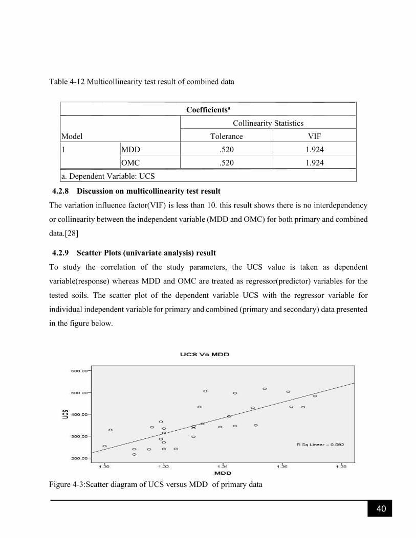
40
Table 4-12 Multicollinearity test result of combined data
Coefficientsa
Model
Collinearity Statistics
Tolerance VIF
1 MDD .520 1.924
OMC .520 1.924
a. Dependent Variable: UCS
4.2.8 Discussion on multicollinearity test result
The variation influence factor(VIF) is less than 10. this result shows there is no interdependency
or collinearity between the independent variable (MDD and OMC) for both primary and combined
data.[28]
4.2.9 Scatter Plots (univariate analysis) result
To study the correlation of the study parameters, the UCS value is taken as dependent
variable(response) whereas MDD and OMC are treated as regressor(predictor) variables for the
tested soils. The scatter plot of the dependent variable UCS with the regressor variable for
individual independent variable for primary and combined (primary and secondary) data presented
in the figure below.
Figure 4-3:Scatter diagram of UCS versus MDD of primary data
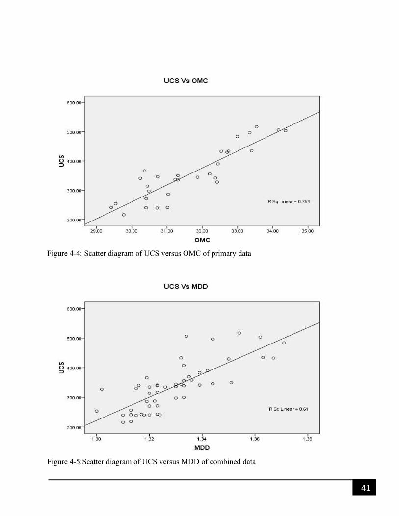
41
Figure 4-4: Scatter diagram of UCS versus OMC of primary data
Figure 4-5:Scatter diagram of UCS versus MDD of combined data

42
Figure 4-6:Scatter diagram of UCS versus OMC of combined data
Figure 4-7:Matrix plot of dependent and independent variable for primary data
450
350
250
343230
1.381.351.32
1.38
1.35
1.32
450350250
34
32
30
UCS
MDD
OMC
Matrix Plot of UCS, MDD, OMC

43
Figure 4-8: Matrix plot of dependent and independent variable for combined data
4.2.10 Descriptive statistics results
The statistical information’s of the test results are presented in table 4.13 and table 4.14
450
350
250
343230
1.381.351.32
1.38
1.35
1.32
450350250
34
32
30
UCS
MDD
OMC
Matrix Plot of UCS, MDD, OMC

44
Table 4-13: Statistical Information of Dependent and Independent Variables for primary data
Table 4-14: Statistical Information of Dependent and Independent Variables for combined data
Descriptive Statistics
N
Minimu
m
Maximu
m Mean
Std.
Deviatio
n
Varianc
e Skewness Kurtosis
Statisti
c Statistic Statistic
Statisti
c
Std.
Erro
r Statistic Statistic
Statisti
c
Std.
Erro
r
Statisti
c
Std.
Erro
r
UCS 50 215.94 516.79
336.79
3
11.3
9 80.5844
6493.86
8 .581 .337 -.266 .662
MDD 50 1.30 1.37 1.329 .002 .01609 .000 .784 .337 .389 .662
OMC 50 29.42 34.36 31.379 .183 1.2985 1.686 .378 .337 -.701 .662
Valid
N(listwis
e)
50
4.2.11 Discussion on the descriptive statistics result
From the above two tables, the result of skewness over its standard error as well as kurtosis over
its standard error is between +2. In appendix A and B the histogram and QQ plot of each variable
Descriptive Statistics
N
Minimu
m
Maximu
m Mean
Std.
Deviatio
n
Varianc
e Skewness Kurtosis
Statisti
c Statistic Statistic
Statisti
c
Std.
Error Statistic Statistic
Statisti
c
Std.
Erro
r
Statisti
c
Std.
Erro
r
UCS 30 215.94 516.79
355.69
1
16.39
7 89.810
8065.97
8 .325 .427 -.894 .833
MDD 30 1.30 1.37 1.332 .003 .01916 .000 .386 .427 -.636 .833
OMC 30 29.42 34.36 31.65 .2529 1.3851 1.919 .255 .427 -.957 .833
Valid
N(listwis
e)
30

45
is shown. The overall result shows each dependent and independent variable is normally
distributed.
4.2.12 Correlation matrix result of data
For determining the influence of one variable on the other, a stepwise linear regression both
forward selection and backward methods using both MINITAB and SPSS software has been used
and the following correlation coefficients and level of significance determined.
Ho: =there is relation between dependent and independent variable
H1: =There is no relation between dependent and independent variable
If there is a relationship between dependent and independent variable α value is less than 0.05 if
not α>0.05. Here under, the Pearson correlation coefficient matrix is shown in Table 4-15 and
Table 4-16 for primary and combined data.
Table 4-15 Correlation Matrix of Pearson Correlation Coefficient for primary data
Correlations
UCS MDD OMC
UCS Pearson Correlation 1 .769** .891**
Sig. (2-tailed) .000 .000
N 30 30 30
MDD Pearson Correlation .769** 1 .709**
Sig. (2-tailed) .000 .000
N 30 30 30
OMC Pearson Correlation .891** .709** 1
Sig. (2-tailed) .000 .000
N 30 30 30
**. Correlation is significant at the 0.01 level (2-tailed).

46
Table 4-16: Correlation Matrix of Pearson Correlation Coefficient for combined data
Correlations
UCS MDD OMC
UCS Pearson Correlation 1 .781** .883**
Sig. (2-tailed) .000 .000
N 50 50 50
MDD Pearson Correlation .781** 1 .693**
Sig. (2-tailed) .000 .000
N 50 50 50
OMC Pearson Correlation .883** .693** 1
Sig. (2-tailed) .000 .000
N 50 50 50
**. Correlation is significant at the 0.01 level (2-tailed).
4.2.13 Discussion of the correlation matrix result
To determine the correlation matrix, Pearson correlation coefficient is selected rather than
spearman correlation coefficient. The reason for this is, the data is continuous as well as the
dependent variable full fill the normality test assumption for both primary and combined data.
Based on the above correlation result, α value is less than 0.05 and Pearson correlation coefficient
value is close to 1. These shows, the data accept null hypothesis and there is a linear relationship
between UCS with maximum dry density and optimum moisture content.
4.2.14 Single Linear Regression Analysis
Model A- 3: Correlation Between UCS and optimum moisture content (OMC)
After correlating UCS with OMC, the following correlation developed.
UCS = - 1473 + 57.8 OMC with R-Sq = 79.4% R-Sq(adj) = 78.7% N=30
UCS = - 1383 + 54.8 OMC with R-Sq = 78.0% R-Sq(adj) = 77.6% N =50
The details of the statistical out-put indicates that the relationship developed between OMC and
UCS is significant (α<0.05) and the detail shown on Appendix D and F
Model A- 4: Correlation Between UCS and maximum dry density (MDD)
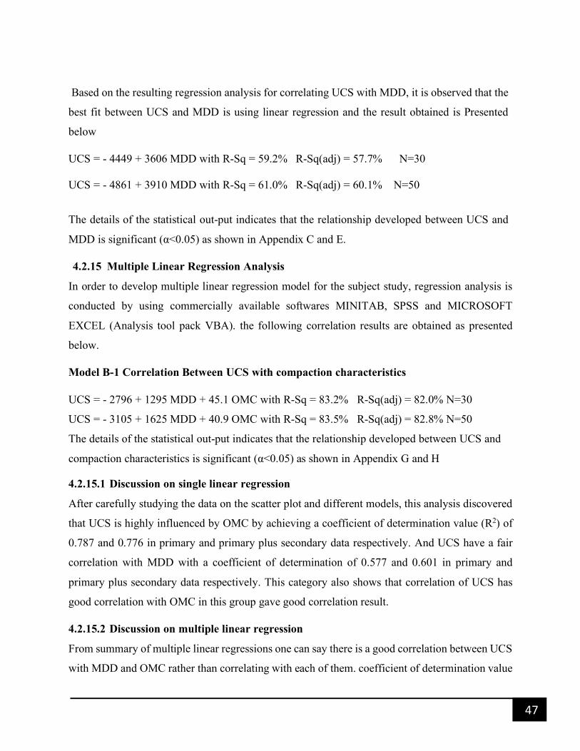
47
Based on the resulting regression analysis for correlating UCS with MDD, it is observed that the
best fit between UCS and MDD is using linear regression and the result obtained is Presented
below
UCS = - 4449 + 3606 MDD with R-Sq = 59.2% R-Sq(adj) = 57.7% N=30
UCS = - 4861 + 3910 MDD with R-Sq = 61.0% R-Sq(adj) = 60.1% N=50
The details of the statistical out-put indicates that the relationship developed between UCS and
MDD is significant (α<0.05) as shown in Appendix C and E.
4.2.15 Multiple Linear Regression Analysis
In order to develop multiple linear regression model for the subject study, regression analysis is
conducted by using commercially available softwares MINITAB, SPSS and MICROSOFT
EXCEL (Analysis tool pack VBA). the following correlation results are obtained as presented
below.
Model B-1 Correlation Between UCS with compaction characteristics
UCS = - 2796 + 1295 MDD + 45.1 OMC with R-Sq = 83.2% R-Sq(adj) = 82.0% N=30
UCS = - 3105 + 1625 MDD + 40.9 OMC with R-Sq = 83.5% R-Sq(adj) = 82.8% N=50
The details of the statistical out-put indicates that the relationship developed between UCS and
compaction characteristics is significant (α<0.05) as shown in Appendix G and H
4.2.15.1 Discussion on single linear regression
After carefully studying the data on the scatter plot and different models, this analysis discovered
that UCS is highly influenced by OMC by achieving a coefficient of determination value (R2) of
0.787 and 0.776 in primary and primary plus secondary data respectively. And UCS have a fair
correlation with MDD with a coefficient of determination of 0.577 and 0.601 in primary and
primary plus secondary data respectively. This category also shows that correlation of UCS has
good correlation with OMC in this group gave good correlation result.
4.2.15.2 Discussion on multiple linear regression
From summary of multiple linear regressions one can say there is a good correlation between UCS
with MDD and OMC rather than correlating with each of them. coefficient of determination value
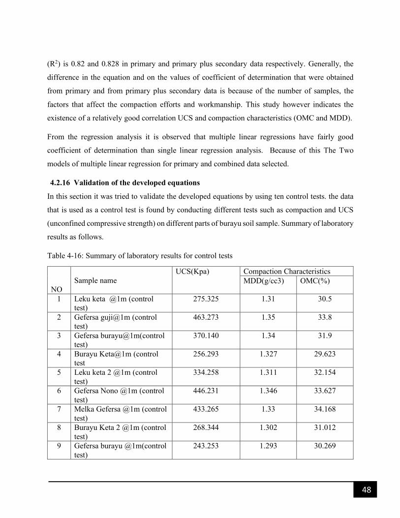
48
(R2) is 0.82 and 0.828 in primary and primary plus secondary data respectively. Generally, the
difference in the equation and on the values of coefficient of determination that were obtained
from primary and from primary plus secondary data is because of the number of samples, the
factors that affect the compaction efforts and workmanship. This study however indicates the
existence of a relatively good correlation UCS and compaction characteristics (OMC and MDD).
From the regression analysis it is observed that multiple linear regressions have fairly good
coefficient of determination than single linear regression analysis. Because of this The Two
models of multiple linear regression for primary and combined data selected.
4.2.16 Validation of the developed equations
In this section it was tried to validate the developed equations by using ten control tests. the data
that is used as a control test is found by conducting different tests such as compaction and UCS
(unconfined compressive strength) on different parts of burayu soil sample. Summary of laboratory
results as follows.
Table 4-16: Summary of laboratory results for control tests
NO
Sample name
UCS(Kpa) Compaction Characteristics
MDD(g/cc3) OMC(%)
1 Leku keta @1m (control
test)
275.325 1.31 30.5
2 Gefersa guji@1m (control
test)
463.273 1.35 33.8
3 Gefersa burayu@1m(control
test)
370.140 1.34 31.9
4 Burayu Keta@1m (control
test
256.293 1.327 29.623
5 Leku keta 2 @1m (control
test)
334.258 1.311 32.154
6 Gefersa Nono @1m (control
test)
446.231 1.346 33.627
7 Melka Gefersa @1m (control
test)
433.265 1.33 34.168
8 Burayu Keta 2 @1m (control
test)
268.344 1.302 31.012
9 Gefersa burayu @1m(control
test)
243.253 1.293 30.269

49
10 Gefersa Nono2 @1m (control
test)
344.215 1.324 31.621
among the developed equations the following equation is selected for validation by higher value
of coefficient of determination (R2). The selected model is UCS = - 3105 + 1625 MDD + 40.9
OMC with R-Sq = 83.5% R-Sq(adj) = 82.8% and standard error =61.373).
4.2.16.1 Cross Validation result
For validation test, the selected control test covers 20% of the training data. The following table
shows the percentage of average validation of controlled test.
Table 4-17: Validation result of data
NO Sample name
UCS
(Kpa)
Compaction
Characteristics
Predicted UCS
(Kpa)
variation
in %
MDD(g/
cc3)
OMC(
%)
1
Leku keta @1m (control
test)
275.3
25 1.31 30.5
271.2 1.498
2
Gefersa guji@1m (control
test)
463.2
73 1.35 33.8
471.17 1.705
3
Gefersa
burayu@1m(control test)
370.1
4 1.34 31.9
377.21 1.910
4
Burayu Keta@1m
(control test
256.2
93 1.327 29.623
262.9557 2.600
5
Leku keta 2 @1m (control
test)
334.2
58 1.311 32.154
340.4736 1.860
6
Gefersa Nono @1m
(control test)
446.2
31 1.346 33.627
457.5943 2.547
7
Melka Gefersa @1m
(control test)
433.2
65 1.33 34.168
453.7212 4.721
8
Burayu Keta 2 @1m
(control test)
268.3
44 1.302 31.012
279.1408 4.023
9
Gefersa burayu
@1m(control test)
243.2
53 1.293 30.269
234.1271 3.752
10
Gefersa Nono2 @1m
(control test)
344.2
15 1.324 31.621
339.7989 1.283
average
variation (%) 2.590

50
4.2.17 Discussion on cross validation result
From The Above cross validation result, the total percentage of variation is 2.59%. this indicate
that there is a very good prediction of the values. The reason for this percentage of variation
occurred is due to the location of the test pit different from the samples considered in the
correlation and seasonal variations. Since the soil vary from place to place and season to season,
it may have different properties. In general, we can conclude that the statistical regression analysis
shows the correlation may give 97% accuracy in determination of the UCS for controlled tests.
Before using this correlation for practical purpose, it also needs modification with large number
of samples and advanced methods rather than simple correlation analysis.
4.2.18 Evaluation of the Developed and Existing Correlations
Specifically, there is no equation developed to determine UCS from Compaction characteristics
for Burayu town. But Ikeagwuani [4] develop the equation for Nigerian clay soil . This correlation
is chosen because the soil type used for regression analysis is classified under tropical residual soil
and it will perform well for Ethiopian soil. The table below shows the variation between the values
of from current study and Ikeagwuani with actual values.
Table 4-18 Validation of UCS From Correlation Developed with The Actual Test Data
Sample
code MDD OMC
UCS
actual
Current
Studies variation
Ikeagwuani
studies variation
1 1.31 29.77 215.943 241.343 11.7624 261.1 20.91154
2 1.32 29.417 240.998 243.155 0.89515 300.2 24.56535
3 1.3 29.54 253.955 215.686 15.0692 222 12.58294
4 1.32 30.44 314.103 284.996 9.26671 300.2 4.426255
5 1.316 30.241 340.637 270.357 20.632 284.56 16.46239
6 1.319 30.361 366.051 280.14 23.4697 296.29 19.05773
7 1.31 30.403 240.236 267.233 11.2376 261.1 8.684793
8 1.32 30.407 270.912 283.646 4.70053 300.2 10.81089
9 1.33 30.48 297.224 302.882 1.90361 339.3 14.15633
10 1.315 30.717 239.291 288.2 20.4393 280.65 17.28398
11 1.324 31.013 241.169 314.932 30.5855 315.84 30.96211
12 1.319 31.032 286.22 307.584 7.46412 296.29 3.518273
13 1.33 31.23 336.84 333.557 0.97465 339.3 0.730317

51
14 1.302 32.42 327.745 336.728 2.74085 229.82 29.87841
15 1.333 32.21 355.946 378.514 6.34029 351.03 1.381108
16 1.32 31.317 335.023 320.865 4.22589 300.2 10.39421
17 1.339 32.373 341.724 394.931 15.5701 374.49 9.58844
18 1.342 32.441 389.993 402.587 3.22926 386.22 0.967453
19 1.33 31.864 344.344 359.488 4.39781 339.3 1.464814
20 1.344 30.73 346.119 335.857 2.96488 394.04 13.84524
21 1.351 31.307 349.74 370.831 6.03057 421.41 20.49237
22 1.334 34.164 505.929 460.058 9.06677 354.94 29.84391
23 1.354 33.541 516.787 467.077 9.61907 433.14 16.18597
24 1.362 34.362 503.365 513.656 2.0444 464.42 7.73693
25 1.367 32.54 432.729 447.261 3.35822 483.97 11.84136
26 1.332 32.745 433.398 398.771 7.98977 347.12 19.90734
27 1.344 33.343 496.635 442.729 10.8543 394.04 20.65803
28 1.35 32.703 429.519 426.303 0.74881 417.5 2.798246
29 1.363 33.4 434.613 475.935 9.50777 468.33 7.757936
30 1.371 32.992 483.557 472.248 2.33875 499.61 3.319774
Figure 4-9 Graphical comparison of the developed model with previous correlations
From table and figure above, one can see that there is variation of UCS by 0.7% to 30% using
Ikeagwuani soil. This indicate that correlation developed for a certain soil is not applicable for
other soil. The reason for this variation is may be due to the difference in test procedures and also
the unique properties of the geological material where this correlation was developed.
-90
10
110
210
310
410
510
610
-3 2 7 12 17 22 27 32
UC
S a
ctu
al (
Kp
a)
Sample Number
actual UCS
Current studies
IKeagwuani

52
CHAPTER -FIVE
5 CONCLUSION AND RECOMMENDATION
5.1 Conclusions
The research was conducted to study correlation between Unconfined compression test or
undrained shear strength (UCS) value and Compaction characteristics. About thirty samples
extracted from the town and laboratory tests were carried out. Using this test results, statistical
analysis was carried out. A single and multiple linear regressions were conducted for both primary
and combined (30 primary and 20 secondary) data and a relationship was developed that predict
the UCS values of a soil in terms of MDD, and OMC
From the results of this study the following conclusions are drawn:
Ø The data results fulfil the basic assumption of normality test and statistical test to conduct
hypothesis testing.
Ø The independent variable maximum dry density and optimum moisture content have less
interdependency between them. The result of multicollinearity is very minimum
Ø From the single linear regression, it is observed that the effect of maximum dry density and
optimum moisture content have positive effect on UCS. That means if maximum dry density and
optimum moisture content tends to increase, the UCS value tends to increase. Therefore, from this
it can be concluded that the increment of dry density and optimum moisture content increase the
strength of undrained shear strength (UCS) soil.
Ø From the single linear regression analysis, the correlation between UCS and optimum
moisture content (OMC) as well as UCS and maximum Dry density (MDD) have fulfil the
objective of thesis by created strong relationship between each other. which was expressed in the
following relationship:
UCS = - 1473 + 57.8 OMC with R-Sq = 79.4% R-Sq(adj) = 78.7% N=30
UCS = - 1383 + 54.8 OMC with R-Sq = 78.0% R-Sq(adj) = 77.6% N =50
UCS = - 4449 + 3606 MDD with R-Sq = 59.2% R-Sq(adj) = 57.7% N=30
UCS = - 4861 + 3910 MDD with R-Sq = 61.0% R-Sq(adj) = 60.1% N=50

53
Ø From the multiple regression analysis, the correlation between UCS and compaction
parameters is used as given below:
UCS = - 2796 + 1295 MDD + 45.1 OMC with R-Sq = 83.2% R-Sq(adj) = 82.0% N=30
UCS = - 3105 + 1625 MDD + 40.9 OMC with R-Sq = 83.5% R-Sq(adj) = 82.8% N=50
From the result combined data gives better correlation than primary data.
Ø From control tests the predicted UCS have an average variation of 2.59% compared to the
actual UCS. This indicates the correlation gives better results. to minimize this variation, use large
number of samples and advanced methods rather than simple correlation analysis.
5. From existing correlations Ikeagwuani [4] estimation of the actual UCS value has over
estimated.
5.2 Recommendations for the future
The following points are some of the recommendations given by the researcher in relation to the
subject study:
1. It is advisable to conduct frequent researches in the soil, due to the fact that soil
property vary from place to place and seasonally
2. Further detailed laboratory analysis carried out on a number of additional disturbed
and undisturbed samples from different locations of the town to prepare a reliable
correlation and regression analysis.
3. Finally, it is important to study Ethiopian soil using advanced other than using
simple regression analysis by collecting different soil property data’s available in to
national database system for further study.

54
REFERENCE
1. Blahova, K., Influence of water content on the shear strength parameters of clayey soil in
relation to stability analysis of a hillside in brno region. 2013. 81(6).
2. Budhu, M., Soil mechanics and foundations. 3rd ed. 2011, United States of America: John
Wiley & Sons, Inc. .
3. Addis, K., Correlation between standard penetration test with unconfined compressive
strength and index properties of fine-grained soil, in Civil Engineering. 2016, Addis Ababa
University: Addis Ababa.
4. Ikeagwuani, c.e.a., Correlation between maximum dry density and cohesion of remoulded
nsukka clays. Nigerian Journal of Technology, 2018. 37.
5. Arora, k.R., soil mechanics and foundation engineering. 2003, Delhi: standard publishers
distributors.
6. Sorensen, K.K.a.O., N. , Correlation between drained shear strength and plasticity index
of undisturbed over consolidated clays, in 18th International Conference on Soil Mechanics
and Geotechnical Engineering. 2013: Paris.
7. Dino, A., A Study on Correlation of California Bearing Ratio (CBR) With Index Properties
of Soils on Welkite –Arekit-Hossana Road., in School of Civil and Environmental
Engineering. 2016: Jimma University.
8. Das, B., Principles of Geotechnical Engineering. 7th ed. 2010: Stamford: Cengage
Learning.
9. Murthy, V.N.S., Soil Mechanics and Foundation Engineering. 5th ed. 2001, new york:
UBS Publishers Distributors Ltd.
10. Bowels , J., Foundation Analysis And Design. 5th ed. 1997, Singapore: McGraw-Hill.
11. Teferra, A.a.L., M, Soil Mechanics. 1999, Addis Ababa Addis Ababa University.
12. Briaud, J.L., Geotechnical Engineering: Unsaturated and Saturated Soils. 2013, United
States of America: John Wiley & Sons, Inc.
13. Das, B., Advanced Soil Mechanics. 3rd ed. 2008., new York , USA: Taylor & Francis e-
Library,.

55
14. Tesfamichael, T., correlation between compaction characteristics and atterberg limits of
fine grained soil found in Addis Ababa. International Journal of Scientific & Engineering
Research, 2017. 8(6).
15. Raju , V., Srimurali, M. and Prasad ,K., Functional Correlations between Compaction
Characteristics, Un-drained Shear Strength and Atterberg Limits. IOSR Journal of
Mechanical and Civil Engineering, 2014. 11(3).
16. Persson, E., Empirical correlation between undrained shear strength and preconsolidation
pressure in Swedish soft clays, in Civil and Architectural Engineering. 2017, Royal
Institute of Technology: Stockholm.
17. Obasi, N.L., Anyaegbunam, A. J., correlation of the undrained shear strength and plasticity
index of tropical clays Nigerian Journal of Technology, 2005. 24(2).
18. Dirriba, A., Developing Correlation between Dynamic Cone Penetration Index (DCPI) and
Unconfined Compression Strength (UCS) of the Soils in Alem Gena Town, in Civil
Engineering (Geotechnical Engineering). 2017, Addis Ababa University.
19. ASTM, Standard Test Method for Laboratory Determination of Water (Moisture) Content
of Soil and Rock by Mass, in D 2216 – 98. 1998: West Conshohocken.
20. Krishna, R., Engineering Properties of Soils Based on Laboratory Testing. UIC, 2002.
21. Hirpassa, W., Investigation on the engineering properties of soil found in burayu town in
Civil Engineering. 2015, Addis Ababa University.
22. Baecher, G.B., Christian,J.T, Reliability and Statistics in Geotechnical Engineering. 2003,
England: John Wiley & Sons Ltd.
23. patel, J.K., Read,C.B, Handbook of the Normal Distribution 1982, New York: Marcel
Dekker, Inc.
24. Berkman, E.T., Reise,S.P, A conceptual guide to statistics using SPSS. 2012, United States
of America: SAGE Publications, Inc.
25. Elliott, A.C., Woodward,W.A, Statistical analysis quick reference guidebook. 2007.
26. Graybill, F., Iyer, H.k., Regression analysis concepts and application. 1962, California:
wadsworth publishing company.

56
27. Yan, X., Su, G.X., Linear Regression Analysis: Theory and Computing. 2009, Singapore:
World Scientific Publishing Co. Pte. Ltd.
28. Stevens , P., Applied Multivariate Statistics For The Social Sciences. 2009, New York:
Taylor & Francis.
29. Montgomery, D.C., Runger, G.C., Applied Statistics and Probability for Engineers. 2002,
United States of America: John Wiley & Sons, Inc.
30. Draper, N.R., Smith, H, Applied Regression Analysis. 1998, United States of America:
John Wiley & Sons.inc.
31. James, G., Witten,D., Hastei,T., Tibshirnai,T, An Introduction to Statistical Learning.
2013, United States of America.
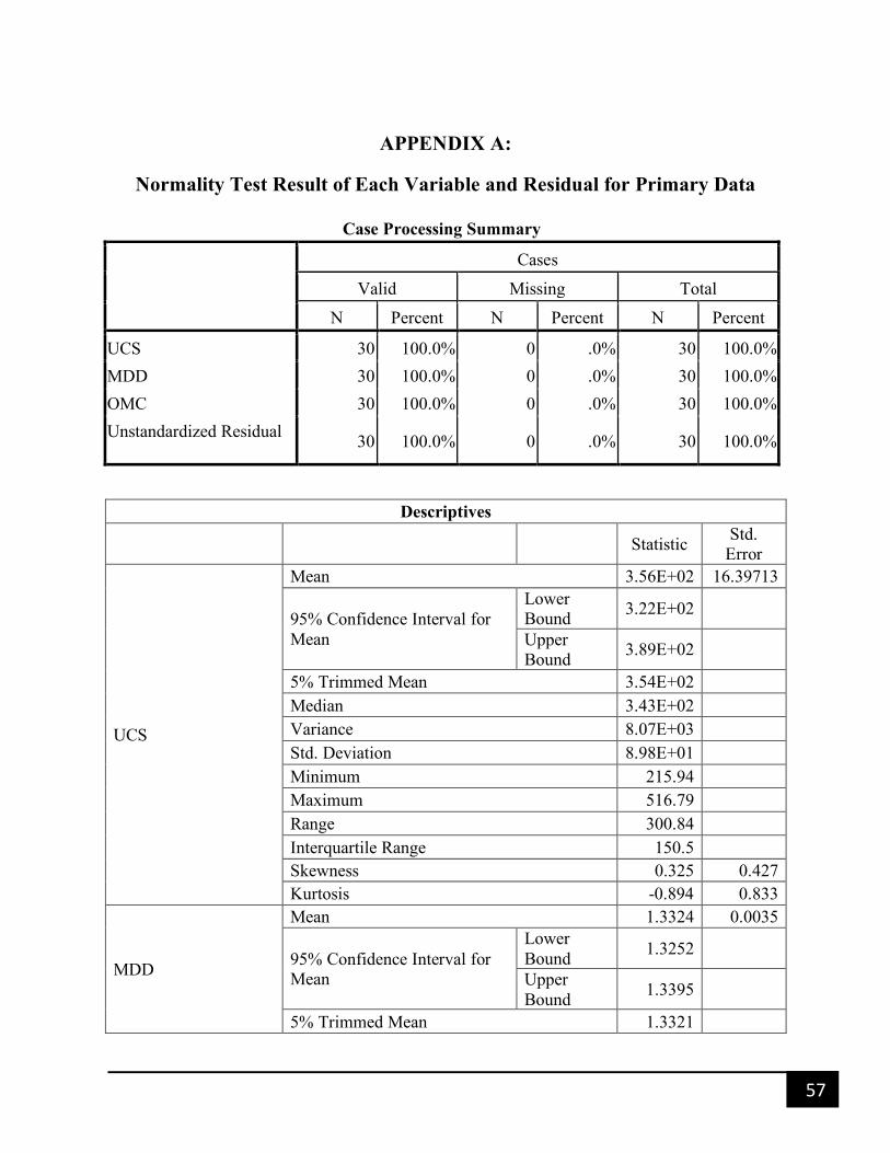
57
APPENDIX A:
Normality Test Result of Each Variable and Residual for Primary Data
Case Processing Summary
Cases
Valid Missing Total
N Percent N Percent N Percent
UCS 30 100.0% 0 .0% 30 100.0%
MDD 30 100.0% 0 .0% 30 100.0%
OMC 30 100.0% 0 .0% 30 100.0%
Unstandardized Residual 30 100.0% 0 .0% 30 100.0%
Descriptives
Statistic Std.
Error
UCS
Mean 3.56E+02 16.39713
95% Confidence Interval for
Mean
Lower
Bound 3.22E+02
Upper
Bound 3.89E+02
5% Trimmed Mean 3.54E+02
Median 3.43E+02
Variance 8.07E+03
Std. Deviation 8.98E+01
Minimum 215.94
Maximum 516.79
Range 300.84
Interquartile Range 150.5
Skewness 0.325 0.427
Kurtosis -0.894 0.833
MDD
Mean 1.3324 0.0035
95% Confidence Interval for
Mean
Lower
Bound 1.3252
Upper
Bound 1.3395
5% Trimmed Mean 1.3321
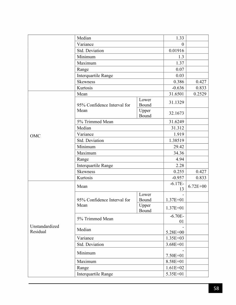
58
Median 1.33
Variance 0
Std. Deviation 0.01916
Minimum 1.3
Maximum 1.37
Range 0.07
Interquartile Range 0.03
Skewness 0.386 0.427
Kurtosis -0.636 0.833
OMC
Mean 31.6501 0.2529
95% Confidence Interval for
Mean
Lower
Bound 31.1329
Upper
Bound 32.1673
5% Trimmed Mean 31.6249
Median 31.312
Variance 1.919
Std. Deviation 1.38519
Minimum 29.42
Maximum 34.36
Range 4.94
Interquartile Range 2.28
Skewness 0.255 0.427
Kurtosis -0.957 0.833
Unstandardized
Residual
Mean -6.17E-
13 6.72E+00
95% Confidence Interval for
Mean
Lower
Bound
-
1.37E+01
Upper
Bound 1.37E+01
5% Trimmed Mean -6.70E-
01
Median -
5.28E+00
Variance 1.35E+03
Std. Deviation 3.68E+01
Minimum -
7.50E+01
Maximum 8.58E+01
Range 1.61E+02
Interquartile Range 5.35E+01

59
Skewness 0.334 0.427
Kurtosis 0.062 0.833
Tests of Normality
Kolmogorov-Smirnova Shapiro-Wilk
Statistic df Sig. Statistic df Sig.
UCS .132 30 .191 .937 30 .077
MDD .141 30 .134 .962 30 .342
OMC .128 30 .200* .957 30 .253
Unstandardized Residual .102 30 .200* .984 30 .918
a. Lilliefors Significance Correction
*. This is a lower bound of the true significance.

60

61
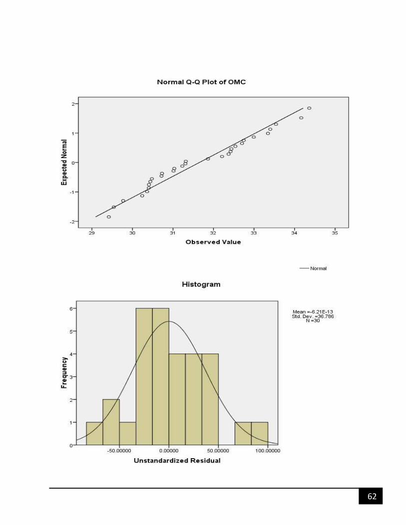
62

63
APPENDIX B:
Normality Test Result of Each Variable and Residual for combined Data
Case Processing Summary
Cases
Valid Missing Total
N Percent N Percent N Percent
ucs 50 100.0% 0 .0% 50 100.0%
mdd 50 100.0% 0 .0% 50 100.0%
omc 50 100.0% 0 .0% 50 100.0%
Unstandardized Residual 50 100.0% 0 .0% 50 100.0%
Descriptives
Statistic Std. Error
ucs
Mean 3.37E+02 11.39638
95% Confidence Interval for Mean
Lower Bound 3.14E+02
Upper Bound 3.60E+02
5% Trimmed Mean 3.34E+02
Median 3.38E+02
Variance 6.49E+03
Std. Deviation 8.06E+01
Minimum 215.94
Maximum 516.79
Range 300.84
Interquartile Range 105.5
Skewness 0.581 0.337
Kurtosis -0.266 0.662
mdd
Mean 1.3293 0.00228
95% Confidence Interval for Mean
Lower Bound 1.3247
Upper Bound 1.3339
5% Trimmed Mean 1.3286
Median 1.325
Variance 0

64
Std. Deviation 0.01609
Minimum 1.3
Maximum 1.37
Range 0.07
Interquartile Range 0.02
Skewness 0.784 0.337
Kurtosis 0.389 0.662
omc
Mean 31.3793 0.18364
95% Confidence Interval for Mean
Lower Bound 31.0103
Upper Bound 31.7484
5% Trimmed Mean 31.3337
Median 31.254
Variance 1.686
Std. Deviation 1.29855
Minimum 29.42
Maximum 34.36
Range 4.94
Interquartile Range 2.03
Skewness 0.378 0.337
Kurtosis -0.701 0.662
Unstandardized Residual
Mean 0 4.63E+00
95% Confidence Interval for Mean
Lower Bound -9.31E+00
Upper Bound 9.31E+00
5% Trimmed Mean -8.41E-01
Median -4.48E+00
Variance 1.07E+03
Std. Deviation 3.28E+01
Minimum -7.21E+01
Maximum 8.76E+01
Range 1.60E+02
Interquartile Range 3.75E+01
Skewness 0.465 0.337
Kurtosis 0.285 0.662
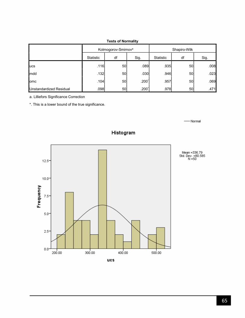
65
Tests of Normality
Kolmogorov-Smirnova Shapiro-Wilk
Statistic df Sig. Statistic df Sig.
ucs .116 50 .089 .935 50 .008
mdd .132 50 .030 .946 50 .023
omc .104 50 .200* .957 50 .069
Unstandardized Residual .098 50 .200* .978 50 .471
a. Lilliefors Significance Correction
*. This is a lower bound of the true significance.
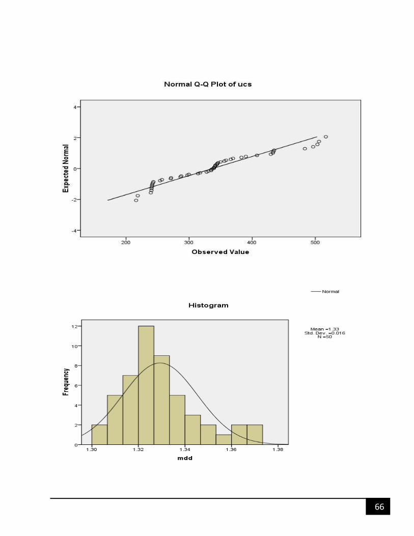
66

67

68
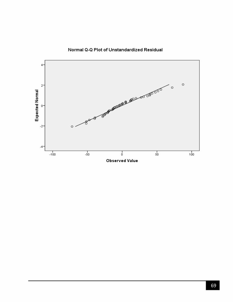
69

70
APPENDIX C:
Single linear regression analysis result between UCS with MDD for primary
Data
Variables Entered/Removedb
Model Variables Entered Variables Removed Method
1 MDDa . Enter
a. All requested variables entered.
b. Dependent Variable: UCS
Model Summaryb
Model R R Square Adjusted R Square
Std. Error of the
Estimate Durbin-Watson
1 .769a .592 .577 58.41172 1.410
a. Predictors: (Constant), MDD
b. Dependent Variable: UCS
ANOVAb
Model Sum of Squares df Mean Square F Sig.
1 Regression 138379.368 1 138379.368 40.558 .000a
Residual 95534.009 28 3411.929
Total 233913.377 29
a. Predictors: (Constant), MDD
b. Dependent Variable: UCS
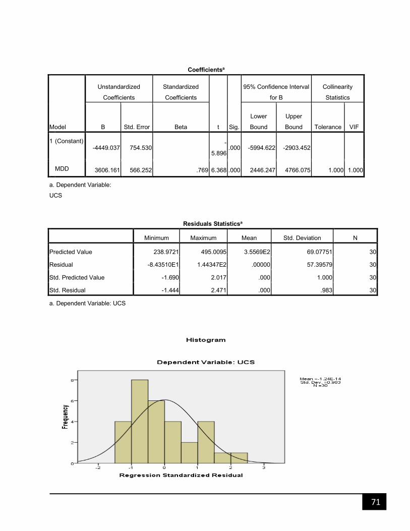
71
Residuals Statisticsa
Minimum Maximum Mean Std. Deviation N
Predicted Value 238.9721 495.0095 3.5569E2 69.07751 30
Residual -8.43510E1 1.44347E2 .00000 57.39579 30
Std. Predicted Value -1.690 2.017 .000 1.000 30
Std. Residual -1.444 2.471 .000 .983 30
a. Dependent Variable: UCS
Coefficientsa
Model
Unstandardized
Coefficients
Standardized
Coefficients
t Sig.
95% Confidence Interval
for B
Collinearity
Statistics
B Std. Error Beta
Lower
Bound
Upper
Bound Tolerance VIF
1 (Constant) -4449.037 754.530
-
5.896 .000 -5994.622 -2903.452
MDD 3606.161 566.252 .769 6.368 .000 2446.247 4766.075 1.000 1.000
a. Dependent Variable:
UCS
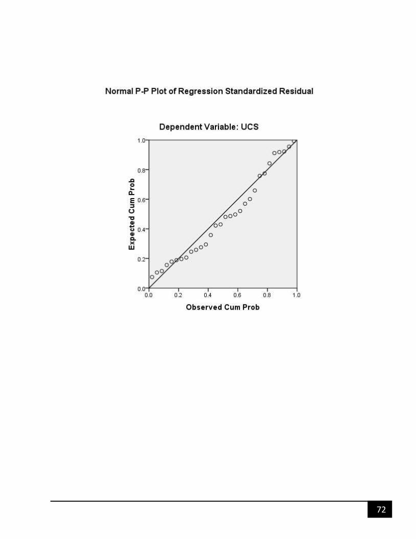
72

73
APPENDIX D:
Single linear regression analysis result between UCS with OMC for primary
Data
Model Variables Entered Variables Removed Method
1 OMCa . Enter
a. All requested variables entered.
b. Dependent Variable: UCS
Model Summaryb
Model R R Square Adjusted R Square
Std. Error of the
Estimate Durbin-Watson
1 .891a .794 .787 41.45385 1.357
a. Predictors: (Constant), OMC
b. Dependent Variable: UCS
ANOVAb
Model Sum of Squares df Mean Square F Sig.
1 Regression 185797.572 1 185797.572 108.121 .000a
Residual 48115.804 28 1718.422
Total 233913.377 29
a. Predictors: (Constant), OMC
b. Dependent Variable: UCS

74
Coefficientsa
Model
Unstandardized
Coefficients
Standardized
Coefficients
t Sig.
95% Confidence
Interval for B
Collinearity
Statistics
B Std. Error Beta
Lower
Bound
Upper
Bound Tolerance VIF
1 (Constant) -1473.199 176.049 -8.368 .000 -1833.820 -1112.578
OMC 57.785 5.557 .891 10.398 .000 46.401 69.168 1.000 1.000
a. Dependent Variable: UCS
Residuals Statisticsa
Minimum Maximum Mean Std. Deviation N
Predicted Value 226.6526 512.3978 3.5569E2 80.04257 30
Residual -7.77079E1 84.84972 .00000 40.73286 30
Std. Predicted Value -1.612 1.958 .000 1.000 30
Std. Residual -1.875 2.047 .000 .983 30
a. Dependent Variable: UCS

75

76
APPENDIX E:
Single linear regression analysis result between UCS with MDD for Combined
Data
Descriptive Statistics
Mean Std. Deviation N
ucs 3.3679E2 80.58454 50
mdd 1.3293 .01609 50
Correlations
ucs mdd
Pearson Correlation ucs 1.000 .781
mdd .781 1.000
Sig. (1-tailed) ucs . .000
mdd .000 .
N ucs 50 50
mdd 50 50
Variables Entered/Removedb
Model Variables Entered Variables Removed Method
1 mdda . Enter
a. All requested variables entered.
b. Dependent Variable: ucs
Model Summaryb
Model R R Square Adjusted R Square
Std. Error of the
Estimate Durbin-Watson
1 .781a .610 .601 50.87485 1.339
a. Predictors: (Constant), mdd

77
Model Summaryb
Model R R Square Adjusted R Square
Std. Error of the
Estimate Durbin-Watson
1 .781a .610 .601 50.87485 1.339
b. Dependent Variable: ucs
ANOVAb
Model Sum of Squares df Mean Square F Sig.
1 Regression 193963.531 1 193963.531 74.940 .000a
Residual 124236.039 48 2588.251
Total 318199.570 49
a. Predictors: (Constant), mdd
b. Dependent Variable: ucs
Coefficientsa
Model
Unstandardized
Coefficients
Standardize
d
Coefficients
t Sig.
95% Confidence Interval
for B
Collinearity
Statistics
B Std. Error Beta
Lower
Bound
Upper
Bound
Toleranc
e VIF
1 (Constant
) -4860.926 600.464
-8.095 .000 -6068.240 -3653.612
mdd 3910.176 451.689 .781 8.657 .000 3001.995 4818.358 1.000 1.000
a. Dependent Variable: ucs
Residuals Statisticsa
Minimum Maximum Mean Std. Deviation N
Predicted Value 222.3031 499.9256 3.3679E2 62.91613 50
Residual -7.49783E1 1.50680E2 .00000 50.35305 50
Std. Predicted Value -1.820 2.593 .000 1.000 50
Std. Residual -1.474 2.962 .000 .990 50
a. Dependent Variable: ucs

78

79
APPENDIX F:
Single linear regression analysis result between UCS with omc for combined
Data
Descriptive Statistics
Mean Std. Deviation N
ucs 3.3679E2 80.58454 50
omc 31.3793 1.29855 50
Correlations
ucs omc
Pearson Correlation ucs 1.000 .883
omc .883 1.000
Sig. (1-tailed) ucs . .000
omc .000 .
N ucs 50 50
omc 50 50
Variables Entered/Removedb
Model Variables Entered Variables Removed Method
1 omca . Enter
a. All requested variables entered.
b. Dependent Variable: ucs
Model Summaryb
Model R R Square Adjusted R Square
Std. Error of the
Estimate Durbin-Watson
1 .883a .780 .776 38.18204 1.478
a. Predictors: (Constant), omc

80
Model Summaryb
Model R R Square Adjusted R Square
Std. Error of the
Estimate Durbin-Watson
1 .883a .780 .776 38.18204 1.478
b. Dependent Variable: ucs
ANOVAb
Model Sum of Squares df Mean Square F Sig.
1 Regression 248221.899 1 248221.899 170.264 .000a
Residual 69977.671 48 1457.868
Total 318199.570 49
a. Predictors: (Constant), omc
b. Dependent Variable: ucs
Coefficientsa
Model
Unstandardized
Coefficients
Standardized
Coefficients
t Sig.
95% Confidence
Interval for B
Collinearity
Statistics
B Std. Error Beta
Lower
Bound
Upper
Bound Tolerance VIF
1 (Constant) -1383.126 131.920 -10.485 .000 -1648.370 -1117.883
omc 54.811 4.201 .883 13.049 .000 46.365 63.256 1.000 1.000
a. Dependent Variable: ucs
Residuals Statisticsa
Minimum Maximum Mean Std. Deviation N
Predicted Value 229.2371 500.2755 3.3679E2 71.17410 50
Residual -7.55458E1 85.07269 .00000 37.79042 50
Std. Predicted Value -1.511 2.297 .000 1.000 50
Std. Residual -1.979 2.228 .000 .990 50
a. Dependent Variable: ucs

81

82
APPENDIX G:
Multiple linear regression analysis result between UCS with MDD and OMC
for primary Data
Variables Entered/Removedb
Model Variables Entered Variables Removed Method
1 OMC, MDDa . Enter
a. All requested variables entered.
b. Dependent Variable: UCS
Model Summaryb
Model R R Square Adjusted R Square
Std. Error of the
Estimate Durbin-Watson
1 .912a .832 .820 38.12366 1.263
a. Predictors: (Constant), OMC, MDD
b. Dependent Variable: UCS
ANOVAb
Model Sum of Squares df Mean Square F Sig.
1 Regression 194671.219 2 97335.609 66.970 .000a
Residual 39242.158 27 1453.413
Total 233913.377 29
a. Predictors: (Constant), OMC, MDD
b. Dependent Variable: UCS

83
Coefficientsa
Model
Unstandardized
Coefficients
Standardized
Coefficients
t Sig.
95% Confidence
Interval for B
Collinearity
Statistics
B Std. Error Beta
Lower
Bound
Upper
Bound Tolerance VIF
1 (Constant) -2796.492 559.488 -4.998 .000 -3944.467 -1648.518
MDD 1294.668 523.965 .276 2.471 .020 219.582 2369.754 .498 2.010
OMC 45.093 7.246 .695 6.223 .000 30.226 59.961 .498 2.010
a. Dependent Variable: UCS
Residuals Statisticsa
Minimum Maximum Mean Std. Deviation N
Predicted Value 218.6358 516.3457 3.5569E2 81.93168 30
Residual -7.49614E1 85.79484 .00000 36.78557 30
Std. Predicted Value -1.673 1.961 .000 1.000 30
Std. Residual -1.966 2.250 .000 .965 30
a. Dependent Variable: UCS
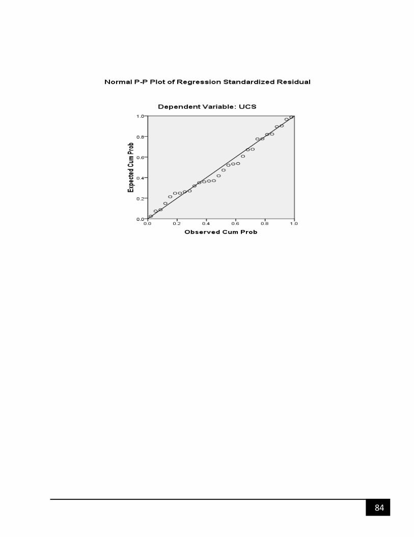
84

85
APPENDIX H:
Multiple linear regression analysis result between UCS with MDD and OMC
for combined Data
Correlations
ucs mdd omc
Pearson Correlation ucs 1.000 .781 .883
mdd .781 1.000 .693
omc .883 .693 1.000
Sig. (1-tailed) ucs . .000 .000
mdd .000 . .000
omc .000 .000 .
N ucs 50 50 50
mdd 50 50 50
omc 50 50 50
Variables Entered/Removedb
Model Variables Entered Variables Removed Method
1 omc, mdda . Enter
a. All requested variables entered.
b. Dependent Variable: ucs
Model Summaryb
Model R R Square Adjusted R Square
Std. Error of the
Estimate Durbin-Watson
1 .914a .835 .828 33.44270 1.328
a. Predictors: (Constant), omc, mdd
b. Dependent Variable: ucs
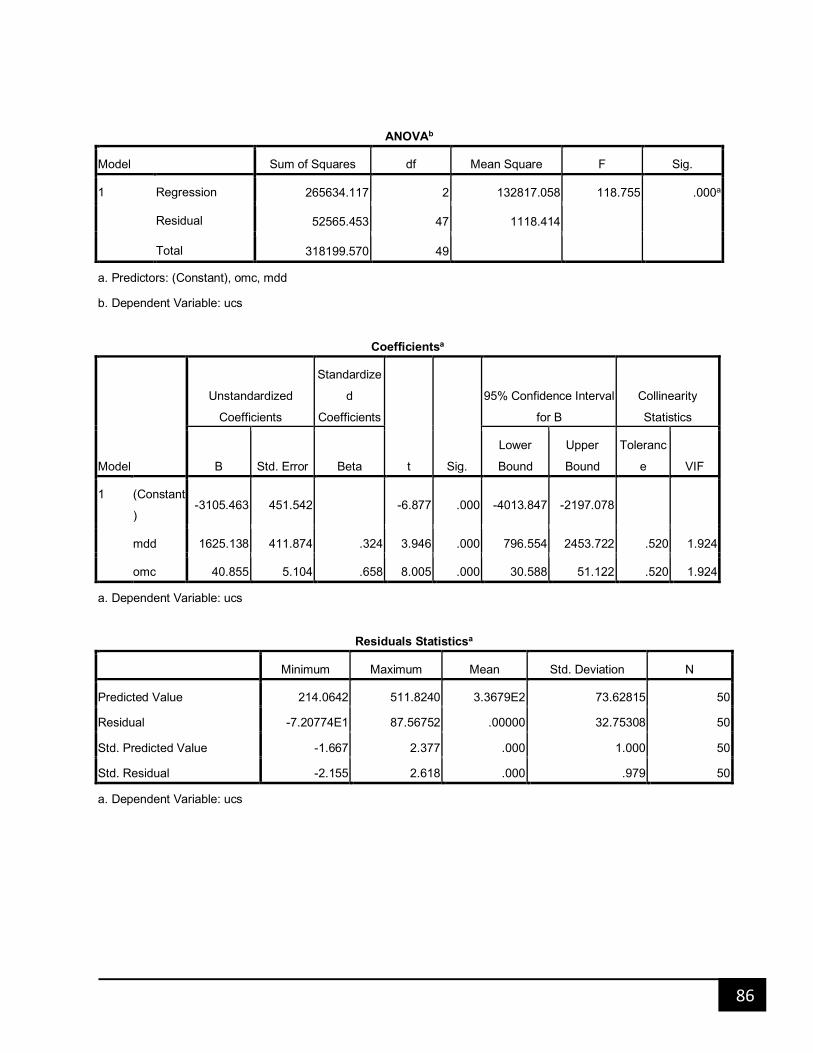
86
ANOVAb
Model Sum of Squares df Mean Square F Sig.
1 Regression 265634.117 2 132817.058 118.755 .000a
Residual 52565.453 47 1118.414
Total 318199.570 49
a. Predictors: (Constant), omc, mdd
b. Dependent Variable: ucs
Coefficientsa
Model
Unstandardized
Coefficients
Standardize
d
Coefficients
t Sig.
95% Confidence Interval
for B
Collinearity
Statistics
B Std. Error Beta
Lower
Bound
Upper
Bound
Toleranc
e VIF
1 (Constant
) -3105.463 451.542
-6.877 .000 -4013.847 -2197.078
mdd 1625.138 411.874 .324 3.946 .000 796.554 2453.722 .520 1.924
omc 40.855 5.104 .658 8.005 .000 30.588 51.122 .520 1.924
a. Dependent Variable: ucs
Residuals Statisticsa
Minimum Maximum Mean Std. Deviation N
Predicted Value 214.0642 511.8240 3.3679E2 73.62815 50
Residual -7.20774E1 87.56752 .00000 32.75308 50
Std. Predicted Value -1.667 2.377 .000 1.000 50
Std. Residual -2.155 2.618 .000 .979 50
a. Dependent Variable: ucs

87

88
Correlations
Approximately 80% of the cases (SAMPLE) UCS predicted
1 UCS Pearson Correlation 1 .916**
Sig. (2-tailed) .000
Sum of Squares and Cross-
products 2.998E5 2.518E5
Covariance 6.663E3 5594.464
N 46 46
predicted Pearson Correlation .916** 1
Sig. (2-tailed) .000
Sum of Squares and Cross-
products 2.518E5 2.518E5
Covariance 5.594E3 5594.481
N 46 46
**. Correlation is significant at the 0.01 level (2-tailed).