Do cument Roompurl .A;IROOM 36-412Restarch Labcratcry C°' o789-.'Masachuse tt s - tt-1-te oc:l r, . .- , .:

CORRELATION FUNCTIONS AND SPECTRAOF MUSIC AND SPEECH

ILAN UYGUR

/LOTECHNICAL REPORT NO. 250

JUNE 15, 1953

RESEARCH LABORATORY OF ELECTRONICSMASSACHUSETTS INSTITUTE OF TECHNOLOGY

CAMBRIDGE, MASSACHUSETTS

I .rrca��rr.r�·li�l(tria�lrCjru�yrrNU~xUiP .'W*�Ki(ii;rU� '.�.·�-"'·'1U"" .·*ri·L�lri.ur�nr. n nrr*·.-.^-�r-··-r.r r·_ --rr· �· -·-rrrl·-�-- -- �-^r·^-��-�-

j d ,.

,W."P

The Research Laboratory of Electronics is an interdepart-mental laboratory of the Department of Electrical Engineeringand the Department of Physics.

The research reported in this document was made possiblethrough support extended the Massachusetts Institute of Tech-nology, Research Laboratory of Electronics, jointly by the ArmySignal Corps, the Navy Department (Office of Naval Research),and the Air Force (Air Materiel Command), under Signal CorpsContract DA36-039 sc-100, Project 8-102B-0; Department ofthe Army Project 3-99-10-022.

-- -_I I � I ___

MASSACHUSETTS INSTITUTE OF TECHNOLOGY

RESEARCH LABORATORY OF ELECTRONICS

Technical Report No. 250 June 15, 1953

CORRELATION FUNCTIONS AND SPECTRA

OF MUSIC AND SPEECH

Ilhan Uygur

This report is substantially the same as a thesis

that was submitted to the Department of Electrical Engineering,

Brown University, May, 1953, in partial fulfillment of the

requirements for the degree of Master of Science.

Abstract

A history of the study of music and speech in the field of communication is given.

The basic ideas and tools in the statistical theory of communication connected to music

and speech are discussed. The electronic technique for performing the necessary math-

ematical operations to obtain the statistical parameters called correlation functions

which yield to spectra are described, with emphasis on the delay problem. The experi-

mental results of a study of music and speech with these methods are presented.

___ __~~~~~

CORRELATION FUNCTIONS AND SPECTRA

OF MUSIC AND SPEECH

I. Introduction

Since the physical characteristics of sound affect its intelligibility and its psycho-

logical properties, technical studies in music and speech are of great importance to

both engineers and psychologists. These characteristics have to be known so that we

can produce, transmit, and reproduce the sound in the most acceptable way.

Since the beginning of the century, many studies have been made dealing with meas-

surements on single notes or vowels (1-22). A summary of earlier studies can be found

in D. C. Miller's book "Science of Musical Sounds". In 1930, a very important experi-

mental study was made at the Bell Telephone Laboratories by Sivian, Dunn, and White

(23, 24). They were interested in making measurements on actual musical selections

and speech, rather than on single notes or vowels, to obtain an average picture of the

selection as well as the distribution of amplitudes in magnitude and frequency. They

used an apparatus in which speech or music spectra were divided into thirteen bands of

frequencies and the power in each of them was measured. These measurements resulted

in a set of curves which have become standard reference data in acoustical engineering

literature for the absolute amplitudes and spectra of speech and music.

Since then, the rapid growth of electronic technique has provided very powerful tools

for the measurement, recording, and reproduction of sound; tools that have revolu-

tionized acoustic technique. In the last decade another useful tool, although perhaps not

so obvious, has been discovered in the realm of statistical communication theory.

Earlier studies of sound did not have the advantages of these tools. In this study,

the writer will try to show how he has attempted to apply methods of statistical commu-

nication theory to the study of music and speech.

Communication can be defined as "any form of transmission of information". The

information which is to be transmitted cannot be considered as a known function of time

because it would be completely specified by its amplitude and phase spectrum or by one

complete period; and once this is known, the continuation of its transmission would not

convey any new information. Thus, when we have a flow of information, it has to be a

random function of time, that is, a statistical phenomenon. This analysis shows one

that all communication problems are statistical in nature. This idea was developed by

N. Wiener (25-27), who is among the many contributors in recent years to the develop-

ment of the new theory of communication, in which the methods and the techniques of

statisticians have been applied.

The branch of the statistical theory which is applicable to communication problems

is the theory of random processes. In this branch of the theory, the most useful

and complete statistical parameters are probability distributions and correlation func-

tions. The probability distributions are more inclusive than the correlation functions

-1-

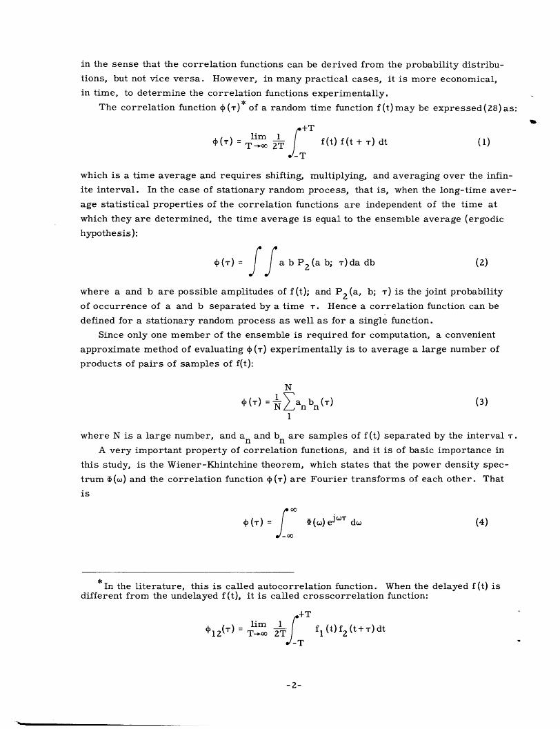
in the sense that the correlation functions can be derived from the probability distribu-

tions, but not vice versa. However, in many practical cases, it is more economical,

in time, to determine the correlation functions experimentally.

The correlation function +(T)* of a random time function f(t)may be expressed(28)as:

+Tlim 1

+(T) = lT-oim I f(t) f(t + T) dt (1)

-T

which is a time average and requires shifting, multiplying, and averaging over the infin-

ite interval. In the case of stationary random process, that is, when the long-time aver-

age statistical properties of the correlation functions are independent of the time at

which they are determined, the time average is equal to the ensemble average (ergodic

hypothesis):

(T)= j a b P2 (a b; T)da db (2)

where a and b are possible amplitudes of f(t); and P 2 (a, b; T) is the joint probability

of occurrence of a and b separated by a time T. Hence a correlation function can be

defined for a stationary random process as well as for a single function.

Since only one member of the ensemble is required for computation, a convenient

approximate method of evaluating (T) experimentally is to average a large number of

products of pairs of samples of f(t):

N

(T) anbn(T) (3)1

where N is a large number, and a n and bn are samples of f(t) separated by the interval T.

A very important property of correlation functions, and it is of basic importance in

this study, is the Wiener-Khintchine theorem, which states that the power density spec-

trum (w) and the correlation function (T) are Fourier transforms of each other. That

is

~ (T) = (c) eWT d (4)

In the literature, this is called autocorrelation function. When the delayed f(t) isdifferent from the undelayed f(t), it is called crosscorrelation function:

lim 2 T f+ T

1( T) lim 1 fl (t) f2 (t+ T) dt

-T

-2-

(W) = , (f ) e jT dT (5)

These relations indicate immediately that knowing the correlation function of a time

function is in every sense equivalent to knowing the power density spectrum.

The well-known Fourier theories of spectrum analysis are not applicable, as they

stand, to random functions such as music and speech. It is possible to obtain the spec-

tra of random functions only with an extension of the Fourier integral theory (32). Then

the power density spectrum can be written (29) as:

T 2

() lim w |1 fT(t)et- t (6)~() =T- oo T 2n T(t)

where fT(t) is a section of duration 2T of the random function f(t). This is a very tedi-

ous task even when one takes advantage of short cuts (28). Therefore, in cases in which

random function's are involved, the indirect determination of the power spectrum through

the use of correlation functions is frequently the most convenient procedure.

The practical application of statistical theory of communication is a result of the

tremendous development of electronic methods during World War II and the development

of Wiener's prediction and filter theory in 1942. By then, electronic techniques were

sufficiently advanced so that this new theory could be applied to the study of some impor-

tant communication problems such as improvement of signal-to-noise ratio, bandwidth

reduction, the lowering of power requirements for the transmission of given messages,

and so on. These problems were either very difficult or impossible to handle with the

conventional theory of communication. Statistical studies started in different groups

(30-33). While one group at the Bell Laboratories was working principally on the the-

oretical side of these problems, the M.I.T. Research Laboratory of Electronics formed

a group to work on their experimental aspects. One of the earliest experimental devices

was an analog correlator (34) which proved the feasibility of high-speed electronic com-

putation of correlation functions. But the requirement for great accuracy and stability,

and especially for very long storage, indicated the need for digital techniques. The out-

come of this was a digital correlator (35). That was followed by a short-time correlator

for speech waves (36), another analog correlator (37), and a five-channel analog corre-

lator (38). At the same time, experimental studies were progressing on the problem of

measuring various probability distributions of random functions (39).

Today, one can find many people applying the methods and concepts of mathematical

statistics to the study of the basic principles of communication.

Statistics may be characterized briefly as the science of reduction and analysis of

observational materials. Any scientific treatment of a given material demands the intro-

duction of a certain order into the material dealt with. Order demands classification;

therefore, any given science is faced by the problem of classifying the available material

-3-

_·

according to some principle. The question then arises, What shall this principle be ?

There is no one definite principle available a priori that would enable one to make a clas-

sification suitable for every purpose.

Many people in the past brought order to the field of music and speech by studying it

from the angle of power spectra, amplitude distributions, zero crossings, and the like.

In this study, the writer tried, with the aid of statistical tools, to bring some order to two

questions which are of interest to communication engineers.

The questions are these:

1. When a musically trained person listens to a sample of music, he can usually

recognize whether it belongs to the classical period or to the romantic period, and even

identify its composer. In other words, musicians have a classification for types of com-

position. One asks, Is it possible to make a music classification of the same kind or of

a different kind with the aid of one of its statistical parameters, the correlation function

in this case ?

2. A study of speech has been made at the M.I.T. Research Laboratory of Elec-

tronics by using the statistical technique (40). The correlation functions of a male and

a female voice reading different passages from a current magazine have been calculated.

These functions have different shapes. Our question is, How different would these curves

be if the same person read samples from different languages, or from different kinds

of literature (prose or poetry) in the same language, or if different persons read the same

literature ?

The results are presented in the next section.

-4-

0

4r)0od >- 0

2 .

o

CA O-

" 4 4 -)

U

.. 0

CO 0

QQ$HCk J

V i

on N

(2)

.:

0c)

UL

0U

0

(.LA>dO

oU

0

, oC 0cdLAO

C-m

-5-

_ _I

-6

T(mSEG)

Fig. 4

Correlation curve of orchestra playing a rhythmic classic selection(Mozart, Piano Concerto in E Flat, final movement).

P

r (mSEC)

Fig. 5

Correlation curve of orchestra playing a melodic classic selection(Mozart, Eine Kleine Nachtmusik, second movement).

-6-

AA

l

80

z60

-

I 1220 440 880 1760CPS

T(mSEC)

Fig. 6

Correlation curve of piano playing a rhythmic polyphonic selection(Bach, Piano Concerto in F Minor, final movement).

CPS

Fig. 7

Correlation curve of piano playing a rhythmic classic selection(Beethoven, Sonata in F Minor, first movement).

-7-

___ I

4

I,

220 440 880 1760CPS

T (mSEC)

Fig. 8

Correlation curve of piano playing a rhythmic romantic selection(Chopin, Polonaise in A Major).

40-

27 ) 220 440 880 1760CPS

I r o - D cam [ o(mSEG)

Fig. 9

Correlation curve of piano playing a melodic polyphonic selection(Bach, Prelude No. 22 for Well-Tempered Clavier).

-8-

80

z 60

m40cr

I ILi

I i i . . I .

I: .I I1 1L 1Q I"

80

10

90

80

70

60

50

40

30

10

z 60

40

a 20

f

Ii27 55 IIC

I I I I I I I I I I I I IV 1 2 3 4 5 6 7

T (mSEGC

Correlation curve(Beethoven,

0 220CPS

440 880 1760

8 9 10 II 12 13 14

Fig. 10

of piano playing a melodic classic selectionSonata in C Minor, second movement).

60[

z I L040 I-ND

w

s

220 440 880 1760P.220 440 880 1760CPS

T (mSEC)

Fig. 1 1

Correlation curve of piano playing a melodic romantic selection(Chopin, Nocturne in D Flat).

-9-

_ _�

r

·--

L ii

I 3 4 0 b ( 8 9 l II1 Iz 3 14 b1 lbr(mSEC)

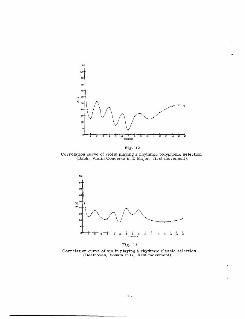
Fig. 12

Correlation curve of violin playing a rhythmic polyphonic selection(Bach, Violin Concerto in E Major, first movement).

90

80

70

60

1P 50

G40

30

20

10

I I I I I I I I I I I I i i" 1 2 3 4 5 6 7 8 9 10 11 12 13 14 15 16

r (mSEC)

Fig. 13

Correlation curve of violin playing a rhythmic classic selection(Beethoven, Sonata in G, first movement).

-10-

--

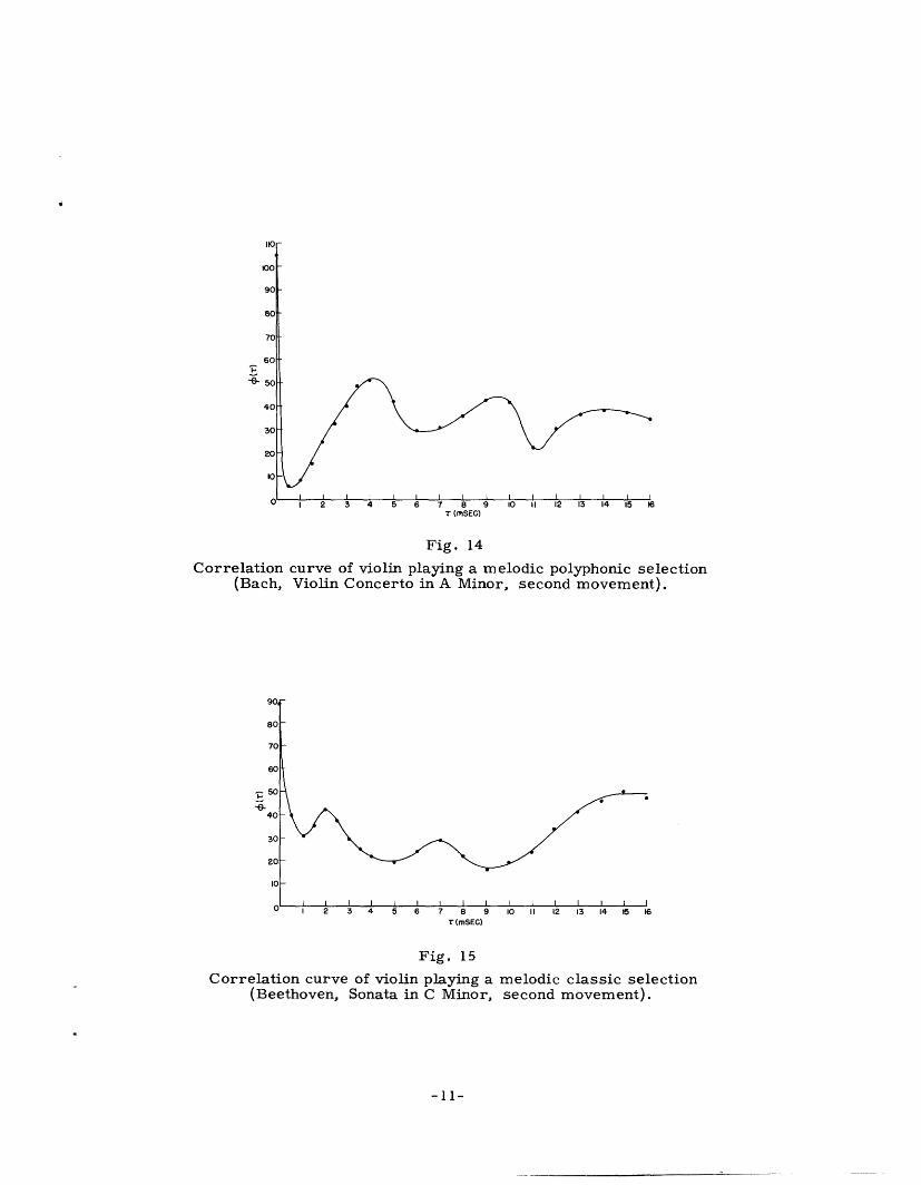
Fig. 14

Correlation curve of violin playing a melodic polyphonic selection(Bach, Violin Concerto in A Minor, second movement).

T (mSEC)

Fig. 15

Correlation curve of violin playing a melodic classic selection(Beethoven, Sonata in C Minor, second movement).

-11-

- -~

5

II. Results

There are many ways that one can plan a study of this nature. The procedure that

appealed the most to the writer was the following.

For music, three periods were chosen: polyphonic, classic, and romantic. A typi-

cal composer from each period was taken, and a rhythmic and a melodic composition

from each composer were selected. The recordings of these selections were obtained

under the same conditions. Then they were analyzed by obtaining their correlation

functions.

For speech, three readers were taken; the first with a monotone voice, the second

with a foreign accent, and the third with a regular voice and good accent. They all read

separately the same prose and the same poetry in English. Then the third reader read

passages from two different classes of languages; in this instance, German and Russian.

Recordings of these readings were made under the same conditions. Then they were

analyzed by obtaining their correlation functions.

This study of music started with orchestral selections. Since records are recorded

under differing conditions, that is, in different halls with different reverberation times,

with different microphones and amplifiers of different frequency responses, with dif-

ferent musicians and conductors, it is obvious that records could not have been used

for this study. Therefore, it was decided that if the concerts of the Boston Symphony

Orchestra playing at Symphony Hall, Boston, Massachusetts, were recorded with the

same equipment, the factors which affected the recordings would be almost the same.

Some of the selections from those recordings were analyzed. The results are the corre-

lation functions shown in Figs. 1-5, all of different character. The study of these

results showed that the field of the study had to be narrowed down; for even though the

recordings were made from the same hall with the same equipment, the seating of the

orchestra was not the same on different days for different compositions. The size of

the orchestra was also different for different works. In order to obtain a much closer

control of the environmental factors, it was decided to narrow down the field of the study

to individual instruments and artists. The instruments chosen were piano and violin.

The selection of rhythmic and melodic compositions for each period was made in such

a way that if a person with no musical training listened to all the rhythmic compositions

from different periods, he would not see much difference between them. In other words,

the selections would appear to be of the same character and period. The correlation

functions of the piano selections are shown in Figs. 6-11. They are, in order, poly-

phonic, classic, and romantic periods. The rhythmic compositions contain more vari-

ations in their correlation functions than the melodic selections. If these variations

have some periodicities, the time interval of the periodicities corresponds to the power

peaks in the frequency domain. For example, the periodicity of approximately 6 msec

of Fig. 10 shows a power peak around 160 cps in the frequency spectrum (see Fig. 32).

There is also a tendency to more variations in the compositions as the periods go from

-12-

�� ·

polyphonic to romantic. Certainly from a limited study of this kind, one cannot come

to definite conclusions. It is easy to see that it will not be simple to recognize the com-

poser or the period of a musical piece by looking at its correlation function. But at least

a correlator will be able to tell, as will a musically untrained person, whether a com-

position has a songlike tempo or a rhythmic and lively one. Maybe the correlators of

the future with built-in memory and capacity to learn will be able to distinguish Bach

from Beethoven.

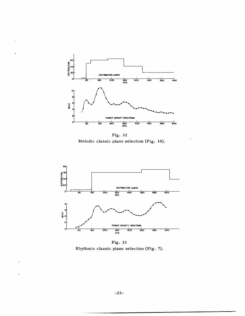
In the right corner of each graph of the piano selections appears a histogram showing

the relative frequency of the pitch, calculated on the basis of four units to a whole note.

This calculation was derived directly from the score of the selection analyzed. The

writer called these histograms "distribution curves". As will be explained later in Figs.

32 and 33, they show the relation between the music and its frequency spectra.

To eliminate completely the effect of any echo from the walls, the recordings of vio-

lin and speech selections were made in the anechoic chamber of the M.I.T. Acoustics

Laboratory. Only selections from polyphonic and classic periods were analyzed for vio-

lin. Their correlation functions are shown in Figs. 12-15. They show the same char-

acteristics as those of the piano selections; that is, the rhythmic compositions have

more variations.

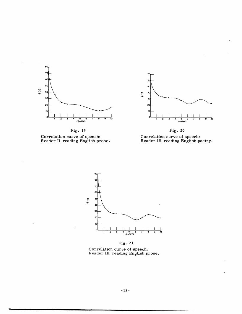
The last part of the study was devoted to speech. Speech correlation functions are

shown in Figs. 16-23. The first reader is the one with a monotone voice (Figs. 16 and

17). The second reader has a foreign accent (Figs. 18 and 19). The third one is a pro-

fessor of modern languages reading English poetry (Fig. 20), English prose (Fig. 21),

German (Fig. 22), and Russian (Fig. 23). The comparison of these curves shows that

the correlation functions or their Fourier transforms, the power density spectra, of

speech waves depend more on the reader than on the language used or the text read. To

find speech waves of this character is of interest, but not surprising. Since the main

physical characteristic of speech, its quality, changes with the resonant pitches of the

throat and mouth cavities, and these characteristics differ from person to person, the

comparison of the curves of the first reader (the monotone voice) with the others shows

clearly how differently pitched voices appear in the correlation functions. The vowel

sounds, which are the low-pitched components of speech, carry most of the energy.

Intelligibility, on the other hand, is largely due to the high-pitched consonants added

by the tongue, teeth, and lips. Difference in languages is formed by a few characteristic

parameters of each language. For instance, an English-speaking person has to differ-

entiate between the sounds " t" and "th". To a Turkish-speaking person, however, that

would not be noticeable. To him, the difference is great between "u" and "u" . Another

difference in languages is found in the sequence of sounds which are mostly influenced

by consonants. Therefore the curves obtained in this study apparently show the influence

of low-pitched vowel sounds of individuals. For the interest of linguists, a further study

in this field would be to remove the consonants from a speech sample tape and then study

it to see how much difference there is from normal speech. A statistical study of just

-13-

__�111 1 __ _· 1�1 _ I� ____1 LU_1 _ _ _

the consonants of a speech sample would also be of interest in the study of languages.

The next problem was to obtain the power density spectra of the selections in which

the greatest number of technical people would be interested. As was shown in the first

section, theory simply states that once the correlation function is known, its Fourier

transform automatically gives its power density spectrum. In this study, the writer was

confronted with some difficulties. Due to technical limitations of the available equip-

ment, which will be explained in section 3, the correlation functions could be calculated

only over a limited range. This fact introduced difficulties to the calculation of their

power density spectra. To see the difficulties more clearly, let us examine Fig. 24.

The part of the correlation function obtained experimentally is shown by f(t); the un-

known end of the function, by g(t); and the assumed zero level of the function (the square

of the mean value), by h. Since the computing circuits of the machine do not handle

negative numbers, the input to the computer is biased to make it all positive. We call

this bias k. And the correlation function obtained from the computer will be

N

D= E [f(t) + K] [fi(t + T) + K]

i=l

N N N

D = fi(t)fi(t+ T)+K f.t)K f(t+ )+ NK 2 (7)

i=l i=l i=l

D1 = N(T) + 2 NK f(t) + NK2

which is N (number of samples) times the correlation function with a constant [2NK f(t)

+ NK 2 ] added to it.

To find the zero level of the correlation function as T goes to infinity, let us corre-

late* the function f(t) with a constant K (for simplicity, this K is taken the same as the

bias K):

N

D = E [fi(t) tk] Ki=l 1

N

D2 = fi(t)K + NK 2

i=l (8)

D 2 = KN f(t)+ NK 2

N f(t)= - NK

*Credit to Dr. A. Fleisher, of the Meteorology Department, Massachusetts Instituteof Technology.

-14-

__ I ___

Then [N f(t)j] would give the value of the zero level of the correlation function as the

output of the computer.

If we subtract Eq. 8 from Eq. 7, we obtain

D1 - D Z = N~(T) + KN f(t)

From Eq. 7 we have

D1 2+(T) = N K - 2K f(t)

Equation 8 gives us

f(t) = K (N - K2

Then we obtain the actual zero level of the correlation function:

D D -2 1 2 - KL) / - (9)(T) - f(t) -- K

By itself,* the Fourier transform of f(t)

+00

f(t) e - j )t dt (10)

would not exist because of the constant h superimposed on it. The expression

[f(t) - h] eit dt (11)

would be finite and the transform would exist if the value of constant h were calculated.

Even then, the transform would not represent the exact spectrum because, as shown in

section 3.3, g(t) is not known; that is, there is no way of finding out how the function

approaches zero level. For this reason different arbitrary values of h and g(t) have

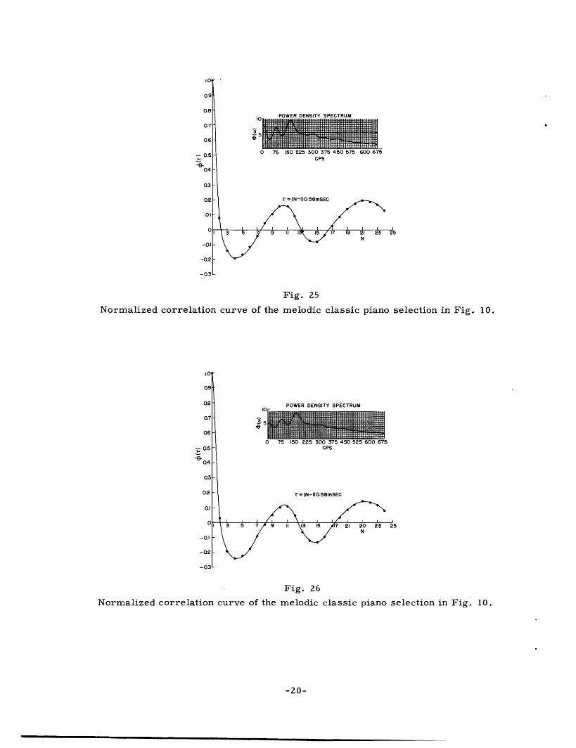
been tried to show the effect of these factors on the spectra. Figures 25-27 show the

power spectrum of Fig. 10 (Beethoven - melodic) for different values of h without the

extrapolation g(t). As the zero level is raised, a constant value is subtracted from the

correlation function which has as its Fourier transform a (sin x/x) curve. The com-

parison of these curves yields the conclusion that the last curve (Fig. 27) is the one with

the most correct zero level, for it is known that there is not much power around very

low frequencies. Figures 28-31 show the spectrum of the same composition for differ-

ent h and g(t). It is obvious that the extrapolation of the correlation functions to zero

The transform is taken from 0 to oo because the correlation functions are symmet-rical about the zero axis.

-15-

level smooths out the power density spectrum. Figures 30 and 31 are probably the best

approximations of the power spectrum of the composition studied.

The lower portions of Figs. 32 and 33 show the spectra of melodic and rhythmic

piano compositions of Beethoven obtained through a different machine with the conditions

of Fig. 27. The results of two machines, the first being mechanical and the second

electronic, check very closely. Distribution curves obtained from the music are drawn

on the same figures to the scale of the spectrum to facilitate comparison between them.

One should not forget that in calculating the distribution curves only the fundamental

frequencies of the notes Written in the music are considered; the power density spectra

contain all the harmonics of the fundamentals. A study made in Japan (41) on music

and speech shows that the waveform of the signal usually is rich in harmonic content.

The distribution curves calculated directly from the music, however, should give a good

first-order approximation of the power spectrum.

-16-

I00

90

80

70

608-

50

40

30

20

I0

*vy

90

80

70

60

50

40

30

I I I I I I I I I II

2 3 4 5 6 7 8 9 10r(mSEC)

Fig. 16

Correlation curve of speech:Reader I reading English poetry.

I I I [ ! i I I I II 2 3 4 5 6 r U 9 Iu

T(mSEC)

Fig. 17

Correlation curve of speech:Reader I reading English prose.

12C

II1

10t

9(

8(

7(

i 6(

51

4(

3,

2(

I

a

0

0

0

0

0

0 -

0 1

0

0

I 2 3 4 5 6 7 8 9 I0r(mSEC)

Fig. 18

Correlation curve of speech:Reader II reading English poetry.

-17-

20

---------------

,.^IlU

Ihn

C

70

6C

50

4C

-9-3C

20

IC

I I I I I I I I I II 2 3 4 5 6 7 9 10

r(mSEC)

Fig. 19

Correlation curve of speech:Reader II reading English prose.

80

70

60

*50

40

30

20

I0

_ I I I I I I I II I I I I I I I I II 2 3 4 5 6 7 8 9 10

T(mSEC)

Fig. 20

Correlation curve of speech:Reader III reading English poetry.

I I I I I I I I I I2 3 4 5 6 7 8 9 10

T(mSEC)

Fig. 21

Correlation curve of speech:Reader III reading English prose.

-18

70

60

50

- 40

30ao

20

I0

V I ' ' ' ' ' U I . . . . . . . . .

I . . . . . . . .O

_

anOU*

-A

70

60

50

40

30

I0

_ I I I I I I I I I1 2 3 4 5 6 7 8 9 0

T (mSEC)

Fig. 22

Correlation curve of speech:Reader III reading German prose.

I I I I I I I I I II 2 3 4 5 6 7 8 9 10

T (mSEC)

Fig. 23

Correlation curve of speech:Reader III reading Russian prose.

f(t)

g(t)

_= 4-h·

TIME

Fig. 24

-19-

ru

60

50

40

-8-30

20

I0

U . . . .n a . . . . . . . . .

I ---Y -----e -· -- - - -

On

POWER DENSITY SPECTRUMlu·53' . H t I . =I .-I .= = ==. . ... E --=-- ...... = ==.== E = I.., I . = -.==9 .iii ii = zi zi iii i ii iiiiii iii iii iii ii iii iii1 -ii_ _ i: . ____0_0*____i i~.iiiiiiiiiiii ;iiiiiiiiiiie iiiiii i;e

0 75 150 225 300 375CPS

450 575 600 675

r (N-I)O.58mSEC

N

Fig. 25

Normalized correlation curve of the melodic classic piano selection in Fig. 10.

Fig. 26

Normalized correlation curve of the melodic classic piano selection in Fig. 10.

-20-

·---

E-9-

Fig. 27 Fig. 28

Normalized correlation curves of the melodic classic piano selection in Fig. 10.

c

-C

Fig. 29

Normalized correlation curve of the melodic classic piano selection in Fig. 10.

-21-

-- ---- -

Fig. 30

Normalized correlation curve of the melodic classic piano selection in Fig. 10.

Fig. 31

Normalized correlation curve of the melodic classic piano selection in Fig. 10.

-22-

___ __ _�_ ___ _ __

I

40

POWER DENSITY SPECTRUMi J i i~~~~~~~~~~~~

80 160 240 320CPS

Fig. 32

400 480 560 640

Melodic classic piano selection (Fig. 10).

DISTRIBUTION CURVEI iI

80 160 240 320 400 480 560 640CPS

8

6 -

4-

2POWER DENSITY SPECTRUM

80 160 240 320CPS

400 480 560 640

Fig. 33

Rhythmic classic piano selection (Fig. 7).

-23-

lu

4 6

4

2

80

60

O 40

20

e0

u , _ _ ._I : _

�_ __ - --- -- -- --

a

--i-

IL

I_

III. Techniques

3.1 Apparatus Used

Analog Correlator

A correlator is an electronic machine which evaluates the correlation functions by

performing the operation of the equation

N

+(T) = a nb n (T (3)

1

The analog correlator (37) of the Research Laboratory of Electronics was used in the

first part of this study. The data are fed into this correlator in the form of a voltage.

An amplitude sample, a, is taken from the input, which is stored as a charge on a capa-

citor.

At a time, T, later, a sample, b, is taken and stored on a separate capacitor (see

Fig. 34). Equation 3 indicates that the amplitudes of the input wave during each sam-

pling period are to be multiplied. This is done by generating pulses of heights propor-

tional to amplitude a, and of widths proportional to amplitude b. The area of the

rectangle formed in this way (a X b) is stored on an RC integrator. Then those samples

are discarded and a new pair of samples is taken. The sampling and multiplying pro-

cess is repeated with an interval, T, and each time the product obtained is added to the

cumulative sum in the integrator. After N such products have been obtained, the sum

is recorded and the integrator is discharged. The sum recorded represents the value

of the correlation function for the value of T under consideration. By changing the

value of T, we can obtain as many points on the correlation function as we desire.

The original Miller feedback integrator of the analog correlator had a time constant

of approximately 100 sec. This is large enough, as compared to the time consumed in

computing one point of the correlation curve (about 16 sec for 16, 000 pairs of samples).

But it was not free from drift, and this would mean a difficult future for the type of data

for which the machine was going to be used. Therefore an integrator of the bootstrap

type, with a time constant of 200 sec, using a unity-gain feedback amplifier, was sub-

stituted for the original integrator. Its operation is described in reference (38). The

new integrator was made free from the small drift that it had by replacing carbon resis-

tors with precision resistors, protecting it from draft by placing it in an insulated box,

a, ba b

-- 4 T --PFig. 34T

Fig. 34

-24-

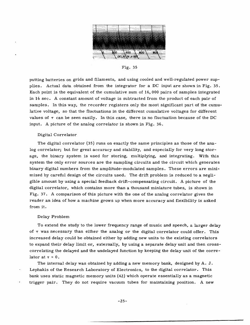
Fig. 35

putting batteries on grids and filaments, and using cooled and well-regulated power sup-

plies. Actual data obtained from the integrator for a DC input are shown in Fig. 35.

Each point is the equivalent of the cumulative sum of 16, 000 pairs of samples integrated

in 16 sec. A constant amount of voltage is subtracted from the product of each pair of

samples. In this way, the recorder registers only the most significant part of the cumu-

lative voltage, so that the fluctuations in the different cumulative voltages for different

values of T can be seen easily. In this case, there is no fluctuation because of the DC

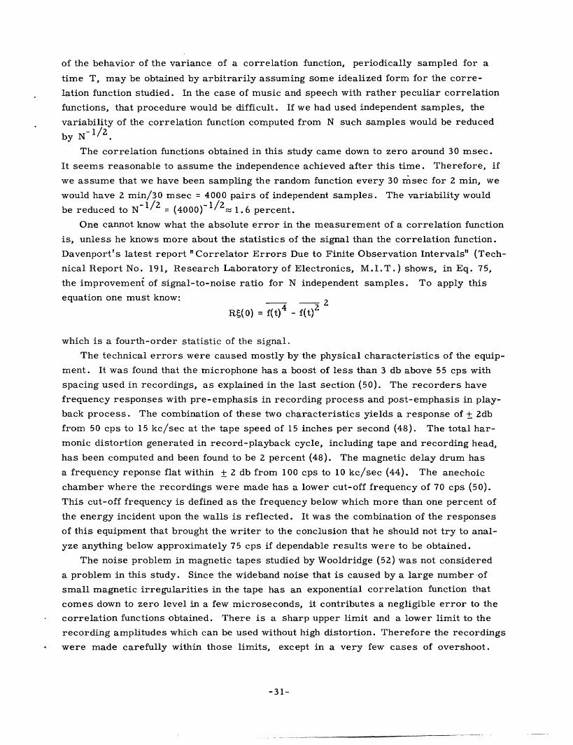
input. A picture of the analog correlator is shown in Fig. 36.

Digital Correlator

The digital correlator (35) runs on exactly the same principles as those of the ana-

log correlator; but for great accuracy and stability, and especially for very long stor-

age, the binary system is used for storing, multiplying, and integrating. With this

system the only error sources are the sampling circuits and the circuit which generates

binary digital numbers from the amplitude-modulated samples. These errors are mini-

mized by careful design of the circuits used. The drift problem is reduced to a negli-

gible amount by using a special feedback drift-compensating circuit. A picture of the

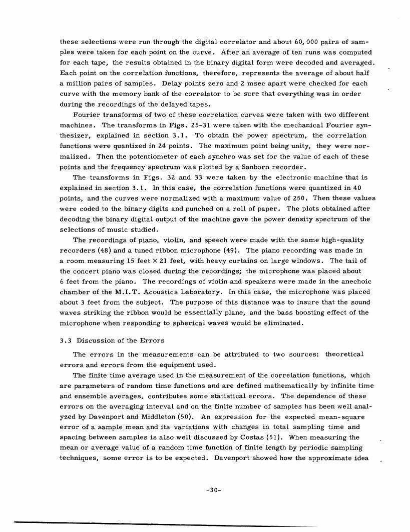
digital correlator, which contains more than a thousand miniature tubes, is shown in

Fig. 37. A comparison of this picture with the one of the analog correlator gives the

reader an idea of how a machine grows up when more accuracy and flexibility is asked

from it.

Delay Problem

To extend the study to the lower frequency range of music and speech, a larger delay

of T was necessary than either the analog or the digital correlator could offer. This

increased delay could be obtained either by adding new units to the existing correlators

to expand their delay limit or, externally, by using a separate delay unit and then cross-

correlating the delayed and the undelayed function by keeping the delay unit of the corre-

lator at T = 0.

The internal delay was obtained by adding a new memory bank, designed by A. J.

Lephakis of the Research Laboratory of Electronics, to the digital correlator. This

bank uses static magnetic memory units (42) which operate essentially as a magnetic

trigger pair. They do not require vacuum tubes for maintaining position. A new

-25-

_··I-··C�.�IC---�II*··-CII�·-r�------� -- I�-- -- - -sl

magnetic material called "Deltamax", having almost a rectangular hysteresis loop, pro-

vides information storage. It also provides the trigger-pair action which depends on

whether the core material is represented by a point on the top of the hysteresis loop or

on the bottom of the loop. The memory bank delays 10 digit binary numbers which cor-

respond to the amplitudes sampled at channel A of the correlator. (See Fig. 38.) Each

of the 10 delay channels consists of 200 static magnetic memory units, connected in a

circuit of the shift-register type. Two units are associated with each of the 100 levels.

The shift pulses are obtained from the correlator timing circuit, and occur at the corre-

lator sampling rate T (see Fig. 34). Each shift pulse causes the contents of the delay

channels to be transferred by one level. During the shifting process all stored pulses

are sent to the crossbar relays, which may be positioned to apply the pulses from any

one of the 100 levels to the output circuit. Stored pulses are lost when shifted out of the

last level. The value of for which a correlation point is computed is equal to the delay

between the pair of samples corresponding to the A and B numbers fed to the multipliers.

Circuits in the correlator are capable of providing delays of from 0.1 sec to approxi-

mately 5 msec. -The memory band provides discrete delays equal to N correlator sam-

pling periods, where N = 1, 2, ... , 100.

In the digital correlator, it takes about 1400 L sec to generate binary digital numbers

from the amplitude-modulated samples, to multiply, and to integrate them. This neces-

sitates starting the minimum sampling period from 2 msec. Therefore even with the

combination correlator's own delay plus the memory bank, which gives the delay in steps

of sampling rate T of the correlator, there is still some gap to be filled in the time

domain.

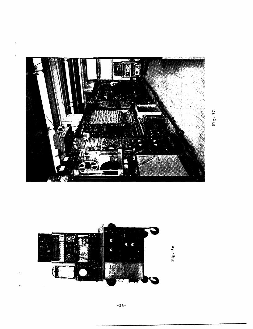
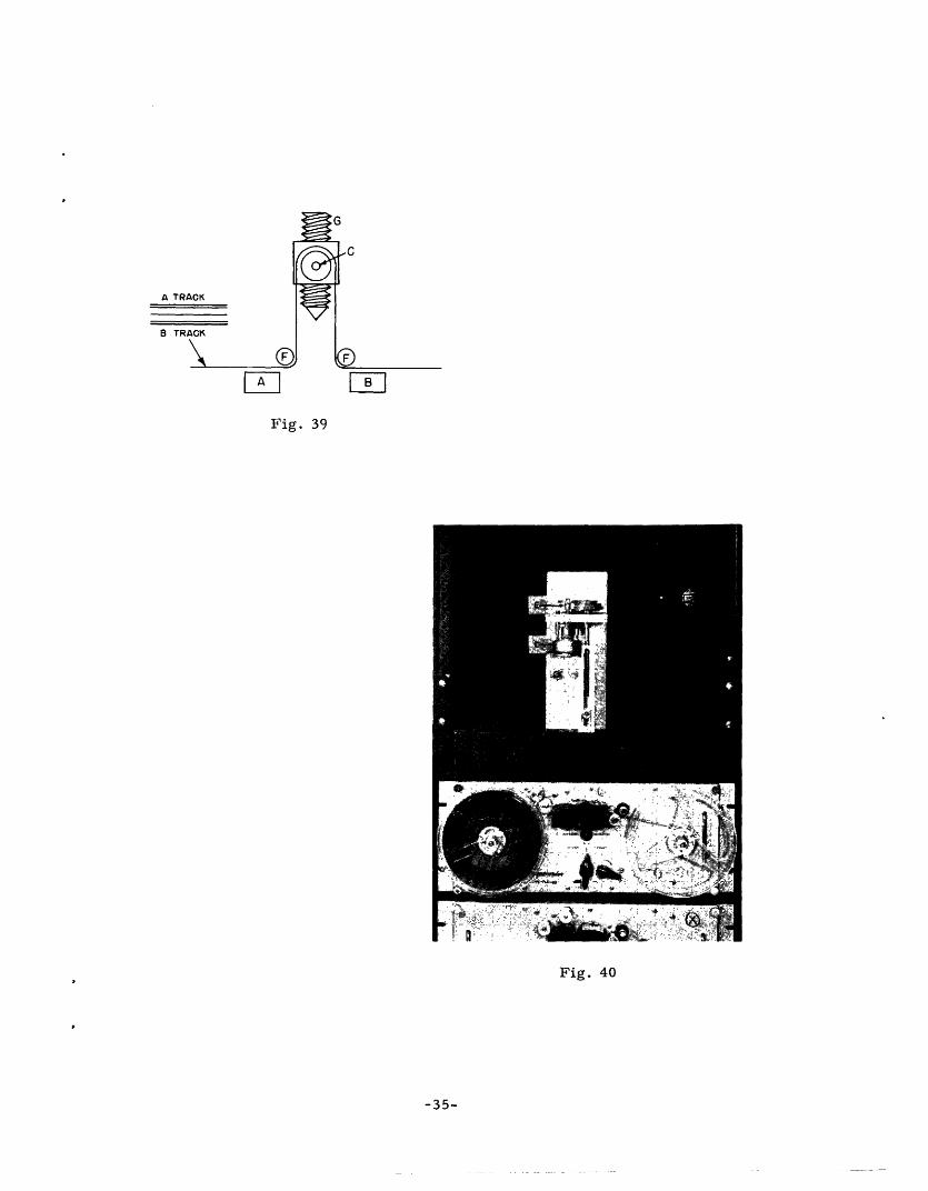
The first idea for obtaining a continuous large delay was to use a twin-track recorder

and give an external delay to one of the tracks (50). The scheme is shown in Fig. 39.

The twin-track recorder records on track A through head A, and on track B through head

B. The position of the pulley C at which the recording is made is a zero-delay position

between the tracks. Turning the threaded rod G clockwise will raise the pulley C and

give delay between the tracks (track B is the delayed one) which can be different for vari-

ous sizes of threads and different speeds of the tape. A picture of the device which was

developed from this idea is shown in Fig. 40, connected to a twin-track magnecorder.

A rotary solenoid D rotates a constant angle when energized. The shaft E of the sole-

noid is connected by gears to the threaded rod. Thus when the rotary solenoid is ener-

gized by the same pulse which resets the correlator at the end of the integration period,

the pulley C is automatically raised by a definite amount which provides the delay. Dif-

ferent gear combinations give different steps, and discrete delays in small intervals up

to seconds can be obtained.

There are some objections to this device. At the speed of 15 inches per sec, the

tape going around the small pulleys F shown in Fig. 39 wears out too fast. These pul-

leys, of approximately 1/8 inch in diameter, were placed there to assure that the mag-

netic face of the tape would make a good contact with the heads. Another criticism is

-26-

__ �

that there is too much tension for the driving mechanism, because the peculiar path of

the tape introduces some distortion to the supposedly constant speed of the tape. This

distortion comes mostly from the slippage in the clutch mechanism. This could be

avoided by adjusting the pressure of the clutch mechanism. Another error is introduced

by the stretching of the tape because of the large pull on it.

In this study, it was thought that these errors could not be considered negligible,

especially in the high frequencies of music. In low frequencies, where the tape could

be run at a slower rate, most of these errors would be very small. The device could

be improved by replacing the small F pulleys with pulleys of larger diameter to smooth

out the track of the tape. That, at the same time, would improve the speed of the tape,

because of the decreased pull on it. The stretching problem of the tape could be solved

by using DuPont's "Mylar" plastic tape, which has a strong coating free from stretching.

The last source of delay was a variable time delay system (44) of the M.I.T. Acous-

tics Laboratory. The main interest of this system is a rotating drum coated with mag-

netic material. The input signal is recorded simultaneously on two tracks of the drum

by techniques similar to those of conventional magnetic recording, and then reproduced

a fraction of a revolution later. The relative time delay between the reproduced signals

is varied by changing the angular spacing between the recording head and the reproducing

head of one channel. This delay drum is much more accurate than the threaded-rod

device because the error problems are not so great.

a) A mechanical driving system is developed with a peak value of flutter as small

as less than 0.02 percent, which is much better than any tape-recording driving mech-

anism.

b) The use of the solid drum coated by a uniform magnetic material, obtained by

spraying with a dispersion of iron oxide, solves the problem of the tape stretch.

Figure 41 shows the drum and its supports. The drum is made 6 inches wide in

order to allow for the addition of other recording tracks in the future, which could be a

good use for a multichannel correlator. The bearings are placed at one end so that the

inside surface of the drum can also be used. The entire drum is machined from Dura-

lumin and the outer surface (8 inches in diameter) runs concentric to within less than

+ 0.1 mil. This accuracy is needed in order to reduce the amplitude modulation of the

signal during recording and reproducing processes. Recording, reproducing, and

erasing heads are spaced a very short distance from the surface of the drum. If they

were run in contact, the surface speed chosen would cause excessive wear on both heads

and magnetic medium. Spacing the heads from the surface of the drum also reduces the

mechanical load on drum drive to that of bearing friction alone, and makes a coupling

system to the driving mechanism more effective in reducing fluctuation in angular vel-

ocity, and thus in delay T. The over-all frequency response of the system is flat

within + 2 db from 100 cps to 10 kc/sec with a 45-db signal-to-noise ratio. The relative

time delay is continuously variable from -15 msec to 190 msec and is calibrated with

an accuracy of + 0.2 percent, or 10 pLsec, whichever is larger.

-27-

___ I

Figure 42 shows the whole system with its power supply and amplifiers.

Computer for Fourier Transforms

The Fourier transforms of two of the correlation functions of music were taken by

a computer (45) to find the power density spectra of these selections.

The computer uses digital inputs and outputs in form of tapes punched in binary code.

The internal operations are in part digital, in part analog. The computer uses the

method of successive approximations based on a fundamental variational principle to

evaluate integral transformation of the Fourier integral. The major mathematical func-

tion performed by the machine is that of transforming on an n vector with an n X n matrix.

The basic errors in this computer come from the following:

a) Interpolation error:

Error committed by interpolating the function space of a problem with a

vector space. (See ref. 45, sec. 6.2)

b) Round-off error:

Error that occurs from computation with a limited number of significant

figures upon data defined to a limited number of significant figures.

c) Machine errors.

The Fourier Synthesizer

The electromechanical synthesizer of the M.I.T. Instrumentation Laboratory (46)

was also used for the transformation of the correlation curves from the time domain to

the frequency domain. This machine consists of an assembly of twenty-four synchros.

The rotors of the synchros are geared together in the ratio 1: 2: 3: ... The output from

each synchro is the voltage induced across a stator winding. The stators can be set in

any angular position to account for the phase angle of the complex exponential term that

it is representing. In this case, they are oriented so that with the phase-angle setting

at zero, the voltage induced across each synchro secondary is proportional to cos a,

where a is the angular position of the rotor. Then this induced voltage is attenuated by

means of a high-precision potentiometer to give the desired magnitude of the complex

exponential term. The attenuated voltages from all the synchros are added electrically.

The resulting voltage is amplified, rectified, and impressed on the galvanometer of a

Sanborn recorder of which the current is proportional to the sum of the cosine voltages.

Since both the synthesizer and recorder are driven at constant speed, the timing line of

the recording paper can be calibrated in terms of angular frequency a, and the trans-

form is obtained as continuous functions of frequency.

3.2 Experimental Procedure

The first problem was to obtain permanent records of the music and speech which

were going to be studied. For the orchestral music, the performances of the Boston

Symphony Orchestra in Symphony Hall, Boston, Massachusetts, were recorded through

-28-

_ _

frequency modulation station WGBH. To obtain good recordings with minimum dis-

tortion, an Ampex tape recorder (47) was used. The next problem was to take pas-

sages from the recorded selections and correlate them. As pointed out in the previous

section, the internal delays of the correlators were too short, and the delay intervals

of the new memory bank were too great. Since the most reliable external delay unit was

the magnetically coated drum, it was employed to solve the delay problem.

The following procedure was used to obtain the delay.

The output of the Ampex recorder was connected to the input of the delay drum. The

outputs of the two heads of the drum, the undelayed and the delayed, were connected to

a twin-track magnecorder. Then the delay of the drum was set to zero, the sample pas-

sage was played on the Ampex magnetic recorder, and was recorded on the twin-track

recorder after going through the delay drum. At the end of the sample passage, the

tapes were stopped on both recorders, the sample tape was rewound to the original

starting point, a delay step of half a millisecond was given to the delay head on the drum,

and the above procedure was repeated. In this way, rolls of two-track magnetic tapes

were obtained with delay intervals of multiples of half a millisecond on each track. The

last delay of each roll of tape was repeated at the beginning of the next roll to correct

the recording levels if there was any difference in the gain of the magnetic materials of

different rolls.

A continuous-loop method was tried for the rewinding of the sample tape, as shown

in Fig. 43. It was found, however, that when a loop of tape longer than 15 feet or 20 feet

was used, the tape (which has one side coated with conducting oxide material, and the

other side with insulating plastic) built up a functional electric charge between layers

of the tape. The charging action resulted in a force which pulled each layer of the tape

to the next one. The attraction between the layers of tape produced an uneven pull on

the drive mechanism of the recorder and in some cases broke the tape. The only rem-

edy for this was to apply a graphite solution on the plastic side of the tape to make it

conducting. This artifice was not satisfactory because of a distortion of the body of the

tape. Therefore the continuous-loop method was not used. A new tape of the Minnesota

Mining Company, which has an aluminum-sprayed plastic back, might be an answer to

this problem, but it is not yet available in the market.

Once the rolls of the tape with delays were prepared, they were fed into the analog

correlator with its delay set at AT = 0. The undelayed track of the tape was fed to the

A channel and the delayed track to the B channel of the correlator. In this way, voltage

coming to the B channel had delay intervals of half a millisecond, and the results

obtained from the correlator at the end of each integration period represented points of

0.5-msec interval on the correlation curve. After the preliminary curves were obtained

on the analog correlator, the data were fed to the digital correlator for the final results.

A block diagram of the whole procedure is shown in Fig. 44. After many experimental

runs, it was found that the sample selections could be reduced to about 2.5 minutes with-

out losing the statistical characteristics of the whole sample. For the final curves,

-29-

__ _1__ 1__11____·__1 _1 1�1_1__

these selections were run through the digital correlator and about 60, 000 pairs of sam-

ples were taken for each point on the curve. After an average of ten runs was computed

for each tape, the results obtained in the binary digital form were decoded and averaged.

Each point on the correlation functions, therefore, represents the average of about half

a million pairs of samples. Delay points zero and 2 msec apart were checked for each

curve with the memory bank of the correlator to be sure that everything was in order

during the recordings of the delayed tapes.

Fourier transforms of two of these correlation curves were taken with two different

machines. The transforms in Figs. 25-31 were taken with the mechanical Fourier syn-

thesizer, explained in section 3.1. To obtain the power spectrum, the correlation

functions were quantized in 24 points. The maximum point being unity, they were nor-

malized. Then the potentiometer of each synchro was set for the value of each of these

points and the frequency spectrum was plotted by a Sanborn recorder.

The transforms in Figs. 32 and 33 were taken by the electronic machine that is

explained in section 3.1. In this case, the correlation functions were quantized in 40

points, and the curves were normalized with a maximum value of 250. Then these values

were coded to the binary digits and punched on a roll of paper. The plots obtained after

decoding the binary digital output of the machine gave the power density spectrum of the

selections of music studied.

The recordings of piano, violin, and speech were made with the same high-quality

recorders (48) and a tuned ribbon microphone (49). The piano recording was made in

a room measuring 15 feet x 21 feet, with heavy curtains on large windows. The tail of

the concert piano was closed during the recordings; the microphone was placed about

6 feet from the piano. The recordings of violin and speakers were made in the anechoic

chamber of the M.I.T. Acoustics Laboratory. In this case, the microphone was placed

about 3 feet from the subject. The purpose of this distance was to insure that the sound

waves striking the ribbon would be essentially plane, and the bass boosting effect of the

microphone when responding to spherical waves would be eliminated.

3.3 Discussion of the Errors

The errors in the measurements can be attributed to two sources: theoretical

errors and errors from the equipment used.

The finite time average used in the measurement of the correlation functions, which

are parameters of random time functions and are defined mathematically by infinite time

and ensemble averages, contributes some statistical errors. The dependence of these

errors on the averaging interval and on the finite number of samples has been well anal-

yzed by Davenport and Middleton (50). An expression for the expected mean-square

error of a sample mean and its variations with changes in total sampling time and

spacing between samples is also well discussed by Costas (51). When measuring the

mean or average value of a random time function of finite length by periodic sampling

techniques, some error is to be expected. Davenport showed how the approximate idea

-30-

__ __

of the behavior of the variance of a correlation function, periodically sampled for a

time T, may be obtained by arbitrarily assuming some idealized form for the corre-

lation function studied. In the case of music and speech with rather peculiar correlation

functions, that procedure would be difficult. If we had used independent samples, the

variability of the correlation function computed from N such samples would be reduced-1/2by N/2

The correlation functions obtained in this study came down to zero around 30 msec.

It seems reasonable to assume the independence achieved after this time. Therefore, if

we assume that we have been sampling the random function every 30 msec for 2 min, we

would have 2 min/30 msec = 4000 pairs of independent samples. The variability would

be reduced to N 1/2 = (4000)-1/2 1.6 percent.

One cannot know what the absolute error in the measurement of a correlation function

is, unless he knows more about the statistics of the signal than the correlation function.

Davenport's latest report "Correlator Errors Due to Finite Observation Intervals" (Tech-

nical Report No. 191, Research Laboratory of Electronics, M.I.T.) shows, in Eq. 75,

the improvement of signal-to-noise ratio for N independent samples. To apply this

equation one must know:4- 2

R(O) = f(t) 4 - f(t) z

which is a fourth-order statistic of the signal.

The technical errors were caused mostly by the physical characteristics of the equip-

ment. It was found that the microphone has a boost of less than 3 db above 55 cps with

spacing used in recordings, as explained in the last section (50). The recorders have

frequency responses with pre-emphasis in recording process and post-emphasis in play-

back process. The combination of these two characteristics yields a response of + 2db

from 50 cps to 15 kc/sec at the tape speed of 15 inches per second (48). The total har-

monic distortion generated in record-playback cycle, including tape and recording head,

has been computed and been found to be 2 percent (48). The magnetic delay drum has

a frequency reponse flat within + 2 db from 100 cps to 10 kc/sec (44). The anechoic

chamber where the recordings were made has a lower cut-off frequency of 70 cps (50).

This cut-off frequency is defined as the frequency below which more than one percent of

the energy incident upon the walls is reflected. It was the combination of the responses

of this equipment that brought the writer to the conclusion that he should not try to anal-

yze anything below approximately 75 cps if dependable results were to be obtained.

The noise problem in magnetic tapes studied by Wooldridge (52) was not considered

a problem in this study. Since the wideband noise that is caused by a large number of

small magnetic irregularities in the tape has an exponential correlation function that

comes down to zero level in a few microseconds, it contributes a negligible error to the

correlation functions obtained. There is a sharp upper limit and a lower limit to the

recording amplitudes which can be used without high distortion. Therefore the recordings

were made carefully within those limits, except in a very few cases of overshoot.

-31-

���___�_I__ __

The errors which could be caused in the correlator by a faulty component were over-

come by running the correlator with a constant input between each point and checking the

results. Since the machine is a digital correlator, the only amplitude drift problem is

in the sampling circuits. The errors of measurement in those circuits have been

reduced by using separate compensators in each channel. (See Fig. 38.) The compen-

sators act to keep the median value of the measured samples at a constant level. They

provide a correction in the number-generating circuits which tends to stabilize the med-

ian value of the binary numbers in the digital parts of the machine.

The effects of synchronization of the input voltage periodicities with the sampling

period of the correlator can be another source of error. If the sampling takes place in

synchronism with a periodic input signal, it can be seen that the first samples of each

pair of samples will always have the same value, depending only on the phase of sam-

pling. In this case, the compensators will adjust the number-generating portions of the

machine to produce the constant median number for the constant magnitude of sample.

If the input samples change to another constant level, the compensators adjust again so

that the same median number results and no change appears in the correlation curve.

The compensators, having a time constant of about 4 sec, make such an adjustment in

a few seconds. These effects of synchronization, however, did not introduce errors to

the functions obtained in this study, because the input signal was not a pure periodic

function of the sampling rate or of any harmonic of the sampling rate.

The characteristics of the various items of the equipment as described above were

considered adequate for the purposes of this study.

-32-

I -- -- - --- _ __I

.0

-33-

I 1_ _11_1· 1_·_1_11__1_____

U)

cn

11l

-34-

�_·

A TRI

B TR,

Fig. 39

, T 'I

Fig. 40

-35-

Fig. 41

Fig. 42

-36-

4 ____ _ ��_ __

- i .-- -, fife ., .

Fig. 43

WGBH SYMPHONYHALL

GHANNEL

Fig. 44

-37-

__ __ _·_ C� _I

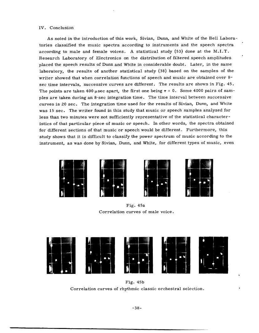
IV. Conclusion

As noted in the introduction of this work, Sivian, Dunn, and White of the Bell Labora-

tories classified the music spectra according to instruments and the speech spectra

according to male and female voices. A statistical study (53) done at the M.I.T.

Research Laboratory of Electronics on the distribution of filtered speech amplitudes

placed the speech results of Dunn and White in considerable doubt. Later, in the same

laboratory, the results of another statistical study (38) based on the samples of the

writer showed that when correlation functions of speech and music are obtained over 8-

sec time intervals, successive curves are different. The results are shown in Fig. 45.

The points are taken 400 sec apart, the first one being T = 0. Some 4000 pairs of sam-

ples are taken during an 8-sec integration time. The time interval between successive

curves is 20 sec. The integration time used for the results of Sivian, Dunn, and White

was 15 sec. The writer found in this study that music or speech samples analyzed for

less than two minutes were not sufficiently representative of the statistical character-

istics of that particular piece of music or speech. In other words, the spectra obtained

for different sections of that music or speech would be different. Furthermore, this

study shows that it is difficult to classify the power spectrum of music according to the

instrument, as was done by Sivian, Dunn, and White, for different types of music, even

Fig. 45a

Correlation curves of male voice.

Fig. 45b

Correlation curves of rhythmic classic orchestral selection.

-38-

_�_

on the same instrument and under the same conditions, give different spectra. It was

also found that the spectrum of speech depends mostly on the reader's voice quality.

Certainly a female voice, having a higher pitch than a male voice, would have power at

higher frequencies. However, this is a classification of a gross character.

The studies of late years show clearly that it is a very difficult problem to transmit

only the intelligence of a message and eliminate its redundance. Through operational

techniques it is possible to eliminate part of the redundance from transmission. This,

however, is usually accompanied by a small loss of information. The future will show

how much progress can be achieved in this direction. Whatever results are obtained,

it is certain that it will never enable us to grasp the problem in its totality any more

than human intelligence will ever rise into the sphere of ideal spirit. However, we have

the right to believe that the progress is real and not aimless. It must be achieved by

filling the gaps. The writer will be happy if this study will fill even the smallest gap.

Acknowledgment

The writer wishes to express his gratitude for the inspiration and advice of Prof.

J. Ruina, of Brown University, under whose supervision this study was carried out.

A study of this nature usually reflects the ideas of many people through the exchange

of views and discussing the problems involved. Therefore a list of such persons would

be long. However, the writer would like to thank Prof. Y. W. Lee for his encourage-

ment throughout the course of the study, and express deep appreciation to the Director

of the M.I.T. Research Laboratory of Electronics, Prof. J. B. Wiesner, for placing

at the writer's disposal the facilities of the laboratory during this study.

The writer is indebted to Mr. L. G. Kraft, Mr. K. Goff, Mr. J. Kessler, Mr. J.

Levin, and Mr. M. Stone for technical assistance. He would also like to acknowledge

the assistance of his artists, Miss D. Bacon and Mrs. E. Fishman, and of his speakers,

Prof. M. Halle, Mr. G. Constantine, and Mr. J. Graham.

-39-

References

1. H. Fletcher: Useful Numerical Constants of Speech and Hearing, Bell System Tech.J., July 1925

2. C. F. Sacia: Speech Power and Energy, Bell System Tech. J., Oct. 1925

3.. C. Stumpf: Characteristic Frequencies for Some Wind Instruments, Zs. f. Phys.,July 1926

4. H. M. Browning: Characteristic Partials of the Violin, Phil. Mag., Nov. 1926

5. N. R. French, W. Koenig: Frequency of Occurrence of Speech Sounds in SpokenEnglish, J. Acoust. Soc. Am., Oct. 1929

6. V. O. Knudsen: The Hearing of Speech in Auditoriums; Average Power of Speakers'Voices in Auditoriums, J. Acoust. Soc. Am., 59-63, Oct. 1929

7. E. Meyer, P. Just: Total Sound Outputs of Several String and Wind Instruments,Zs. f. Tech. Phys., Oct. 1929

8. W. B. Snow: Audible Frequency Ranges of Music, Speech, and Noise, J. Acoust.Soc. Am., July 1931

9. L. J. Sivian, S. D. White: On Minimum Audible Sound Fields, J. Acoust. Soc.Am., April 1933

10. J. Tiffin: Applications of Pitch and Intensity Measurements of Connected Speech,J. Acoust. Soc. Am., April 1934

11. H. Fletcher: Loudness, Pitch and Timbre of Musical Tones, J. Acoust. Soc. Am.,Oct. 1934

12. S. K. Wolf, D. Stanley, W. J. Sette: Quantitative Studies on the Singing Voice, J.Acoust. Soc. Am., April 1935

13. H. Dudley: Automatic Synthesis of Speech, Proc. Nat. Acad. Sci., July 1939

14. H. Dudley: The Carrier Nature of Speech, Bell System Tech. J., Oct. 1940

15. A. W. Ladner: Analysis and Synthesis of Musical Sounds, Electronic Eng'g., Oct.1940

16. O. J. Murphy: Measurements of Orchestral Pitch, J. Acoust. Soc. Am., Jan. 1941

17. K. D. Kryter: Advantages of Clipping the Peaks of Speech Waves Prior to RadioTransmission, Nat. Def. Res. Com. PB22859, Oct. 1944

18. P. Chavasse: Sur une Voix Artificielle pour les Mesures Acoustiques, Compt.rend., June 1947

19. J. C. R. Licklider, D. Bindra, I. Pollack: Intelligibility of Rectangular SpeechWaves, Am. J. Psychol., Jan. 1948

20. J. C. R. Licklider, I. Pollack: Effects of Differentiation, Integration, and InfinitePeak Clipping upon the Intelligibility of Speech, J. Acoust. Soc. Am., Jan. 1948

21. H. Fletcher: Perception of Speech and Its Relation to Telephony, Science, Dec.1948

22. J. W. Black: Natural Frequency, Duration, and Intensity of Vowels in Reading,J. Speech Dis., July-September Quarterly, 1949

23. L. J. Sivian: Speech Power and its Measurement, Bell System Tech. J., Oct. 1929

24. L. J. Sivian, H. K. Dunn, S. D. White: Absolute Amplitudes and Spectra of Cer-tain Musical Instruments and Orchestras, J. Acoust. Soc. Am., Jan. 1931

25. N. Wiener: Generalized Harmonic Analysis, Acta Math. 55, 1930

26. N. Wiener: Cybernetics, John Wiley and Sons, New York

27. N. Wiener: The Extrapolation, Interpolation, and Smoothing of Stationary TimeSeries, John Wiley and Sons, New York

-40-

_____

References (continued)

28. H. M. James, N. B. Nichols, R. S. Phillips: Theory of Servo-Mechanisms,McGraw-Hill, New York and London

29. Y. W. Lee: Application of Statistical Methods to Communication Problems, Tech-nical Report No. 181, Research Laboratory of Electronics, M.I.T., 1950

30. H. K. Dunn, S. D. White: Statistical Measurements on Conversational Speech, J.Acoust. Soc. Am., Jan. 1940

31. G. Sacerdote: Statistical Measures of Vocal Intensity, Ann. Telecommun., March1948

32. D. W. Reed: A Statistical Approach to Quantitative Linguistic Analysis, Word,Dec. 1949

33. S. Chang, G. E. Pihl, M. W. Essigmann: Representation of Speech Sounds andSome of their Statistical Properties, Proc. I.R.E., Feb. 1951

34. T. P. Cheatham, Jr.: An Electronic Correlator, Technical Report No. 122,Research Laboratory of Electronics, M.I.T., 1951

35. H. E. Singleton: A Digital Correlator, Technical Report No. 152, Research Lab-oratory of Electronics, M.I.T., 1950

36. P. E. A. Cowley, R. M. Fano, B. L. Basore: A Short-Time Correlator for SpeechWaves, Technical Report No. 174, Research Laboratory of Electronics, M.I.T.,1951

37. J. F. Reintjes: An Analogue Electronic Correlator, Proc. Nat. Elect. Conf.,Feb. 1952

38. M. J. Levin: A Five-Channel Electronic Analogue Correlator, Master's Thesis,Department of Electrical Engineering, M.I.T., 1952

39. W. B. Davenport, Jr.: A Study of Speech Probability Distributions, TechnicalReport No. 148, Research Laboratory of Electronics, M.I.T., 1950

40. L. G. Kraft: Correlation Function Analysis, J. Acoust. Soc. Am., Nov. 1950

41. J. Obata, R. Kobayashi: Application of Our Direct Reading Pitch and IntensityRecorder, Proc. Phys.-Math. Soc. Japan, March 1941

42. M. Kincaid, J. M. Alden, R. B. Hanna: Static Magnetic Memory for Low-CostComputers, Electronics, Jan. 1951

43. P. E. Green, Jr.: Communication Research, Quarterly Progress Report, ResearchLaboratory of Electronics, M.I.T., Jan. 15, 1951

44. K. W. Goff: Development of a Variable Time Delay, Master's Thesis, Departmentof Electrical Engineering, M.I.T., 1952

45. J. M. Ham: The Solution of a Class of Linear Operational Equations by Methodsof Successive Approximations, Doctoral Thesis, Department of Electrical Engi-neering, M.I.T., 1952

46. R. C. Seamans, Jr., B. P. Blasingame, G. C. Clementson: The Pulse Methodfor the Determination of Aircraft Dynamic Performance, J. Aeronaut. Sci., Jan. 1950

47. Ampex Series 400 Magnetic Recorder Manual, Redwood City, California

48. PT 63-J, PT 6-AH, and PT 6-J Technical Specifications, Magnecord Inc., Chicago,Illinois

49. Radio Corp. of America: Instructions for Velocity Microphone, Type 44-BX, RCAVictor Div., Camden, New Jersey

50. W. B. Davenport, Jr., R. A. Johnson, D. Middleton: Statistical Errors in Meas-urements on Random Time Functions, J. Appl. Phys., April 1952

-41-

_� ___ ____ _ ____ _ I�� ____ _ ·-----------·11�·111IIIIC·

References (continued)

51. J. P. Costas: Periodic Sampling of Stationary Time Series, Technical ReportNo. 156, Research Laboratory of Electronics, M.I.T., 1950

52. D. E. Wooldridge: Signal and Noise Levels in Magnetic Tape Recording, Elec.Eng., June 1946

53. R. S. Berg: Distributions of Filtered Speech Amplitudes, Master's Thesis,Department of Electrical Engineering, M.I.T., 1951

-42-