Correlation Uncertainty, Heterogeneous

Beliefs and Asset Prices

Junya Jiang Weidong Tian∗

September, 2016

∗Belk College of Business, University of North Carolina at Charlotte, Charlotte. Junya Jiang,jjiang6@uncc.edu; Weidong Tian, wtian1@uncc.edu. We thank Jaroslav Borovicka, Ethan Chiang, DicksDavid, Jerome Detemple, Kewei Hou, Tao Li, Jianjun Miao, Philip Illeditsch (discussant), Tan Wang, HongYan, Shunming Zhang (discussant) and the participants in 2016 SFS Finance Cavalcade (Toronto), 2016China International Finance Association (Xiamen).

1

Correlation Uncertainty, Heterogeneous

Beliefs and Asset Prices

Abstract

We construct an equilibrium model in the presence of correlation uncertainty and

heterogeneous ambiguity-averse investors. In this model the level of correlation un-

certainty and asset characteristic jointly affect the asset prices and trading activities.

The price of low weighted volatility asset declines and naive agent holds less posi-

tion when the level of correlation uncertainty goes up; concurrently, the price of high

weighted volatility asset increases and the naive agent holds larger position. The so-

phisticated agent provides liquidity in the market and always holds a well-diversified

optimal portfolio with higher portfolio risk and better performance. Moreover, regard-

less low or high weighted volatility, higher trading volumes are associated with a larger

dispersion of correlation uncertainty across agents. This model explains a number of

well documented empirical puzzles on correlation, including asymmetric correlation,

under-diversification and limited participation, comovement and flight to quality in the

financial market.

2

A principle purpose of research in finance is to study the correlated structure among all

financial assets. Correlated structure is pervasive in financial market and plays a central role

in finance since Markowitz (1952)’s seminal work on the portfolio choice, arbitrage pricing

theory and derivative pricing (Duffie et al, 2009), among many others. However, to estimate

the correlated structure is difficult from both statistical and econometric perspective (Chan,

Karceski and Lakonishok, 1999; Ledoit, Santa-Clara and Wolf, 2003). The challenge to esti-

mate the correlated structure stems from several reasons such as lack of enough market data

source, limitation in estimation methodology, correlation process being unstable or virtually

complicated (Bursaschi, Porchia and Trojani, 2010; Engle, 2002), not to mention the in-

creasingly interconnected market pattern, making the whole correlation analysis much more

demanding than the estimation of the marginal distribution.1 Besides its fundamental role in

asset pricing, numerous studies have empirically documented some significant phenomenons

arising from correlation structure, including asymmetric correlation (Ang and Chen, 2002;

Longin and Solnik, 2001), under-diversification and limited participation (Vissing-Jorgensen,

2002; Calvet, Campbell and Sodini, 2009; Dimmock, Kouwenberg, Mitchell and Peijnenburg,

2016), comovement and contagion (Barberis, Shleifer and Wurgler, 2005; Vedlhamp, 2006;

Kyle and Xiong, 2001), flight to quality and flight to safety (Caballero and Krishnamurthy,

2008; Vayanos, 2004).

The aim of our study is to explain the aforementioned empirical puzzles using a uniform

theoretical model and offer novel predictions for optimal portfolio choice and asset pricing.

We construct an equilibrium model with heterogeneous correlation uncertainty among agents

by employing a multiple-priors setting in Gilboa and Schmeidler (1989).2 Specifically, agents’

concern on the correlated structure is interpreted by ambiguity-aversion on the correlated

structure, or virtually the correlation coefficient estimation. Each agent is risk averse and

1Alternatively, the correlated structure or the covariance matrix can be estimated from the option mar-ket. See Buss and Vilkov (2012); Kitiwiwattanachai and Pearson (2015). However, the complexity of thecorrelation process still preserves in spite of this implied estimation methodology.

2There is a growing body of research in asset pricing that applies the multiple-priors framework. See, forinstance, Easley and O’Hara (2009, 2010); Garlappi, Uppal and Wang (2007); Cao, Wang and Zhang (2005);Uppal and Wang (2003). For other approaches to address the ambiguity and its implication to asset pricing,see Bossaerts, Ghiraradato, Guarnaschelli and Zame (2010); Routledge and Zin (2014) and Illeditsch (2011).

3

ambiguity averse. Agents are heterogeneous in terms of ambiguity aversion, reflecting their

various levels of sophistication to deal with statistical data and estimation methodology.3

To concentrate on the role of correlation ambiguity, we assume that agents have perfect

knowledge of the marginal distributions for all assets; that is, they merely have concerns

about the correlation structure. In this manner, our discussion on the correlation uncertainty

significantly departs from previous literature in model uncertainty where either expected

return or the variance estimation is a concern. For instance, Cao, Wang and Zhang (2005),

Garlappi, Uppal and Wang (2007), Boyle, Garlappi, Uppal and Wang (2012), Easley and

O’Hara (2009) investigate the expected return parameter uncertainty. Easley and O’Hara

(2010), Epstein and Ji (2014) discuss volatility parameter uncertainty. In an information

ambiguity setting, Illeditsch (2011) addresses the conditional distribution ambiguity of the

signals. In all those previous studies, the correlation structure is always given as exogenous.

Instead, allowing ambiguity on the correlation structure while the marginal distribution is

known can cast a situation in which ambiguity-averse agent view the overall market as highly

ambiguous rather than individual stocks (Boyle, Garlappi, Uppal and Wang, 2012; Uppal

and Wang, 2003). In this regard the correlation uncertainty can be also explicated to some

extent as systemic risk uncertainty since the ambiguity on the overall market attributes to

the macroeconomic uncertainty (See Dicks and Fulghieri, 2015).4

In this paper, the unique equilibrium in the presence of correlation uncertainty is char-

acterized in which the optimal correlated structure and the optimal portfolio for each agent

are simultaneously determined. The characterization of the equilibrium demonstrates that

the heterogeneous beliefs in correlation uncertainty, among others, plays a critical role in

characterizing the equilibrium. Specifically, when the dispersion of correlation uncertainty

among agents is small, each agent chooses the highest available correlation in a full partici-

pation equilibrium. On the other hand, when the uncertainty dispersion is large, while the

sophisticated agent still chooses her highest possible correlation coefficient, the naive agent’s

choice of correlation coefficient is no longer relevant in the equilibrium, even though his op-

timal portfolio is unique. We show that this portfolio inertia feature can be obtained in the

3There are both laboratory evidence and non-laboratory empirical evidence of ambiguity aversion hetero-geneity. See Bossaerts, Ghiraradato, Guarnaschelli and Zame, 2010; Dimmock, Kouwenberg, Mitchell andPeijnenburg, 2016.

4Examining the “best” joint distribution with fixed marginal distributions has also been well studied inclassic statistical literature (Strassen, 1965; White 1976).

4

context of both portfolio choice and equilibrium under model uncertainty, and it turns out

that a limited participation equilibrium emerges because of the portfolio inertia property.

In addition to generate the limited participation endogenously through the channel of

correlation uncertainty, we show that the sophisticated agent always holds a more diversified

(well-diversified) portfolio whereas the naive agent holds an under-diversified portfolio. We

confirm that the naive agent’s portfolio is less risky because his higher correlation uncertainty

yields a higher implicit risk aversion.5 We also show that the sophisticated agent achieves a

better performance on the optimal portfolio than the naive agent.

Our portfolio analysis heavily hinges upon a dispersion measure, inspired by the portfolio

selection literature (Hennessy and Lapan, 2003; Ibragimov, Jaffee and Walden, 2011), as we

propose to quantify the dispersion among economic variables. Previous studies on under-

diversification and limited participation such as Cao, Wang and Zhang (2005), Wang and

Uppal (2003), Easley and O’Hara (2009) focus on negligible positions on assets of which

the marginal distribution is ambiguous. In contrast, we examine the optimal portfolio itself

and compare it with a well-diversified market portfolio by using this dispersion measure in

a precise manner. Our portfolio approach to the limited participation is consistent with the

methodology in Calvet et al. (2009), Dimmock et al. (2016), Polkovnichenko (2005) and

Hirsheleifer, Huang and Teoh (2016). We further show that the optimal portfolio is less

diversified with higher perceived level of correlation uncertainty across the agents, which is

empirically documented in Dimmock et al. (2016).

This equilibrium model has several key implications in understanding the stylized facts

about correlation structure. First, correlation asymmetry occurs endogenously. Since an

agent’s correlation ambiguity is often larger in the weak market than in the strong market,

a higher correlation in a downside market movement is obtained in equilibrium. Moreover, a

higher correlation is associated with a higher volatility of individual asset. This correlation

asymmetry phenomenon (Ang and Chen, 2002; Longin and Solnik, 2001) is shown to be

persistent despite the heterogeneity in correlation estimation.

Second, we find that the dispersion of Sharpe ratios decreases endogenously as correla-

tion uncertainty increases regardless of the dispersion in correlation uncertainty. Previous

5See Garlappi, Uppal and Wang (2007); Gollier (2011); Wang and Uppal (2003) for the discussion thatambiguity leads to risk aversion implicitly.

5

studies document that assets moves closely together in a downside market and moves apart

in an upside market (Pindyck and Rotemberg, 1993; Forbes and Rigobon, 2002; Barberis,

Shleifer and Wurgler, 2005). Our model reveals that all risky assets are enforced to comove

more with a higher level of correlation uncertainty, as a result of similar investment opportu-

nities provided in the market. Therefore, our model sheds light to further understand asset

comovement from an investment perspective.

Third, the level of the correlation uncertainty affects asset prices differently based on

asset characteristics. We use individual asset’s weighted volatility over the total weighted

volatility of all assets, which we call as eta in this paper, to measure its relative risk contri-

bution to the entire market while the asset size factor represents the weight. In Appendix

C we demonstrate that the eta characterizes the sensitivity of individual asset return with

respect to the market portfolio return. For a low eta asset, the higher the correlation un-

certainty, the lower the price. Meanwhile, the price of a high eta asset increases as the level

of correlation uncertainty increases. This cross-sectional asset price pattern with respect to

agents’ ambiguity aversion illustrates a significant heterogeneous paradigm. In a homoge-

neous equilibrium, the endogenous correlation coefficient is large when the perceived level of

a representative agent’s correlation uncertainty is large; therefore, one asset’s price decline

reduces the prices of all assets (contagion). Remarkably, a richer price pattern is obtained

for assets with varying characteristics under heterogeneity of correlation uncertainty.

Fourth, the model divulges agents’ trading activities when the level of correlation un-

certainty varies. Each agent holds “long” position on high eta assets, but the naive agent

might “sell” some low eta assets. When the dispersion among agents’ correlation uncertainty

is large or when the ambiguity on the entire market is large, the sophisticated agent’s long

position on the low eta asset increases whereas the naive agent’s corresponding position de-

creases. For very low eta assets, the holding of the naive agent could even be negative (short

positions). In contrast, he holds long positions for high eta assets. Since a high level of corre-

lation uncertainty or a large dispersion among agents’ ambiguity often comes with a stressed

economy, the high eta assets can be used to hedge against the “catastrophic economic shock”

or “correlation uncertainty”. Therefore, we provide an alternative explanation of flight-to-

safety or flight-to-quality episodes because those high eta assets enjoy a high demand from

the naive agent and its price moves up sharply in a very weak economic situation. Studies

6

like Caballero and Krishnamurthy(2007), Vayanos (2004) and Guerrieri and Shimer (2014)

develop a model to generate the flight-to-quality with liquidity risk or adverse selection. Our

model generates flight-to-quality endogenously from a correlation uncertainty perspective.

Finally, the model implies that high trading volume is always associated with high level

of correlation uncertainty or a large dispersion in correlation ambiguity among agents, for

both low eta as well as high eta assets. In a very weak economic situation, the naive agent

is easy to get panic and overreact to the market, thus purchases a significant amount of high

eta assets and sells substantially on low eta assets. When we interpret the heterogeneity as

disagreement, our result justifies theoretically a recent empirical findings in Carlin, Longstaff

and Matoba (2014).

As one application, our theoretical results offer a concrete description about the financial

market during the 2007-2009 crisis. Following Bloom (2009), Baele, Bekaert, Inghelbrecht

and Wei (2013), we use VIX index to measure the ambiguity on the overall financial market.

Figure 1 displays VIX as well as S&P 500 index from 2006 to 2016. As shown clearly, VIX is

extremely high within the whole year of 2008, representing a very high level of uncertainty

in the market. We observe the VIX index and S&P index move in opposite directions

consistently for the entire period from 2006-2016. On the other hand, we compare VIX with

gold price during the same time period 2006-2016, in Figure 2, and we see the gold price is

to a large extent positively correlated to the VIX price. If we define the whole stock market

as one risky asset and other type of assets including fixed income securities, foreign exchange

and commodity market together as another risky asset, we can further argue that the stock

market is a low eta asset class while the financial market excluding the stock market is a

high eta asset class. We present detailed analysis in Section 4.6 Following this interpretation,

the naive agent’s market demand on high eta assets (including bond, hard commodity, in

particular gold and silver market) sharply increases when the perceived level of uncertainty

moves up, and the higher the uncertainty level the larger the positions. Meanwhile, the naive

agent reduce his positions on the low eta assets, i.e. stocks. This analysis explains investors’

flight to safety activities in 2007-2009. Furthermore, the trading volume on both the stock

6Briefly speaking, the volume of the fixed income market alone is about triple size as the stock marketglobally. Since the volatility of stock market is about three times of the fixed-income market, their weightedvolatility is about the same. Adding a comparable size of commodity market and a much larger volume ofthe foreign exchange market into the weighted volatility of non-stock financial market, the eta of the stockmarket is quite small compared to the eta of the non-stock market.

7

market and these uncertainty-hedging asset classes increases significantly if the dispersion of

correlation uncertainty is large, as shown from our model as well as the market data.

The model also highlights important role of sophisticated agents (institutional investors)

on the financial market. With increasing number of institutional investors, naive agents are

more likely to hold a limited participation portfolio and sophisticated agents therefore domi-

nate the trading activities and asset prices. Moreover, each agent’s optimal portfolio perfor-

mance is improved given a large number of sophisticated agents. Hence, introducing more

sophisticated agents into the market, and enhancing investors’ finance education/training

can be beneficial to every investor as well as the whole financial market.7 More importantly,

we show that the premium of low eta asset decreases and the premium of high eta asset

increases because of large number of institutional investor; thus, our model also helps to ex-

plain the disappearance of the small firm premium due to the increased institutional investor

demands (Gompers and Metrick, 2001).

The rest of the paper is organized as follows. Section 1 presents a model setting of

correlation uncertainty. In Section 2, we study the portfolio choice problem under correlation

uncertainty and demonstrate the persistent portfolio inertia feature. We also characterize

the equilibrium in a homogeneous environment as a baseline model. In Section 3 we present

the unique market equilibrium under heterogeneous correlation uncertainty. We explain in

Section 4 the joint effect of correlation uncertainty and asset characteristic on asset price

and risk premium. Section 5 presents the optimal portfolio analysis. We establish that the

sophisticated agent always has a well-diversified, higher risk and better performance optimal

portfolio than the naive agent. The trading activities and trading volumes are examined

carefully in Section 6, in which the effect of the heterogeneity in correlation uncertainty is

discussed extensively. We further investigate the effect of the percentage of sophisticated

agent as well as the dispersion of asset characteristics (eta) on the equilibrium. Section 7

extends the model to a block equicorrelation structure and Section 8 concludes. Proofs and

technical arguments are collected in Appendices.

7Easley and O’Hara (2009) and Easley, O’Hara and Yang (2015) present similar insights from alternativeperspectives.

8

1 A Model of Correlation Uncertainty

There are N risky assets and one risk-free asset which serves as a numeraire in a two-period

economy (date t = 0 and t = 1). The payoffs or dividends of these N risky assets are

a1, a2, · · · , aN , respectively at time t = 1. The risk-free asset is in zero net supply, and

the per capita endowment of risky asset i is xi, i = 1, · · · , N . Each risky asset can be

viewed as an investment asset, an investment fund, an asset class, or a market portfolio in

an international market.

To focus entirely on the correlated risk and its effect on asset pricing, we investigate

the correlation structure instead of the joint distribution of (a1, · · · , aN).8 In other words,

given known marginal distribution of each ai, we study the asset pricing implication within

a plausible set of joint distribution. Since the correlation coefficient between the payoffs is

identical to the correlation coefficient between asset returns, our assumption is equivalent to

the ambiguity purely on asset returns’ correlation structure and the agent has no ambiguous

on the marginal distribution on the asset return; but this marginal distribution is charac-

terized endogenously in our setting. In this paper we confine ourselves on a nonnegative

correlated financial market.9

In our specification of the correlation matrix, we employ Engle and Kelly (2012)’s dy-

namic equicorrelation (DECO) model; that is, any two distinct risky assets have a same

correlation coefficient ρ, i.e., corr(ai, aj) = ρ for each i 6= j.This assumption on the corre-

lation structure will be relaxed in a block equicorrelation model in Section 7. Engle and

Kelly (2012) show that the (block) DECO estimation of U.S. stock return data can display

a better fit for the data than a general dynamic conditional correlation (DCC in Engle,

2002) model. For simplicity, we assume that (a1, · · · , aN) has a multivariate Gaussian dis-

tribution as in Cao, Wang and Zhang (2005), Easley and O’Hara (2009, 2012). That is,

each agent is confident in the estimation of expected mean ai and variance σ2i for each risky

8By a copula theory (see McNeil, Frey and Embrechts, 2015), the joint distribution of a = (a1, · · · , aN ) ischaracterized by the marginal distribution of each ai, and a copula function which determines the correlationstructure. In other words, the correlation structure can be independent of the marginal distributions. Wevirtually assume a parametric single-factor Gaussian copula correlation structure in this paper, but oursetting itself is general enough to encounter an arbitrary copula correlation structure.

9Technically speaking, our results hold when all correlation coefficients are strictly larger than − 1N−1 .

A positive correlated structure is driven by common shocks, or some factors in a financial market. Boththe diversification benefits and synchronization are more critical in a positive correlated economy than in anegative correlated environment.

9

asset i = 1, · · · , N ; however, they are seriously concerned about the estimation of ρ which

represents the ambiguity aversion on the correlated structure.

There is a group of agents in this economy. Each agent has the CARA-type risk prefer-

ence to maximize the worst-case diversification benefit

minρ

Eρ [u(W )] , u(W ) = −e−γW , (1)

where ρ runs through a plausible correlation coefficient region, Eρ[·] represents the expecta-

tion operator under corresponding correlation coefficient ρ, and γ is the agent’s absolute risk

aversion parameter and we assume that each agent has the same absolute risk aversion. In

this regard our setting departs from Ehling and Larsen (2013) which studies the correlation

structure through the channel of heterogeneity in risk aversions.

Every agent encounters some correlation uncertainty, and we assume that the corre-

lation coefficient is a plausible region instead of one particular number. The agents are

heterogeneous in their estimations of the correlation matrix. There are two types of agent,

sophisticated (“she”) and naive (“he”). For the sophisticated agent, her available correlation

coefficient region is [ρ1, ρ1]; while for the naive agent, his correlation coefficient region is

[ρ2, ρ2].10 We assume [ρ

1, ρ1] ⊆ [ρ

2, ρ2], which reflects the fact that the estimation on cor-

relation coefficient for the sophisticated agent is more accurate than the naive agent. The

percentage of sophisticated agents in the market is ν and naive agents’ percentage is 1− ν.

The plausible correlation coefficient region [ρ, ρ] represents the correlation magnitude

as well as uncertainty and its presence can be justified as follows. An agent has in mind

a benchmark or reference correlation coefficient that represents his best estimate on the

correlation, and the benchmark/reference correlation is implied byρ+ρ

2; on the other hand,

the level of correlation uncertainty indicates how far away plausible correlation coefficients

move upon and below the benchmark and this uncertainty is measured byρ−ρ

2. In most

situations, econometricians are able to find the benchmark correlation coefficient through

the calibration to a stochastic matrix process, and treat it as a market reference with some

estimation errors (Buraschi, Porchia and Trojani, 2010; Chan, Karceski and Lakonishok,

10It is well known that the plausible linear correlation coefficient between any two variables X and Y isan interval, [ρmin, ρmax]. See NcNeil, Frey and Embrechts (2015).

10

1999; Engle, 2002). By abuse of notations, we use ρavg to denote the benchmark and ε the

level of uncertainty.

As a special case to notice, both types of agents can agree on the same benchmark

correlation coefficient, but have different ambiguity degrees with respect to the correlation

coefficient estimation. If so, the available correlation coefficient for the sophisticated agent is

[ρavg−ε1, ρavg+ε1], and the naive agent’s plausible correlation coefficient is [ρavg−ε2, ρavg+ε2]

and ε1 < ε2. An extreme situation is ε1 = 0, where the sophisticated agent becomes a Savage

investor with perfect knowledge about the correlation structure.11 We illustrate our results

with these special cases later.

2 Equilibrium in a Homogeneous Environment

We first solve the portfolio choice problem under correlation uncertainty, then present the

equilibrium in a homogeneous environment.

2.1 Portfolio Choices

Let xi be the number of shares on the risky asset i, i = 1, · · · , N , and W0 is the initial wealth

of the agent, then the final wealth at time 1 is

W = W0 +N∑i=1

xi(ai − Pi),

where Pi is the price of the risky asset i at time t = 0. Assuming the plausible range of the

asset correlation coefficient is [ρ, ρ] and there is no trading constraint, the optimal portfolio

choice problem for the agent is

maxx∈RN

minρ∈[ρ,ρ]

Eρ[−e−γW

]. (2)

11Alternatively, by adopting Cao et al. (2005), we can assume that there is a continuum of agents, say[ρavg − ε, ρavg + ε], each type of investor’s correlation uncertainty is captured by the parameter ε while ε isuniformly distributed among agents on [ε − δ, ε + δ] with density 1/(2δ). The main insights of this settingare fairly similar to ours whereas the impact of sophisticated agents in our current setting has a clearerexpression. Our setting is in a manner reminiscent of Easley and O’Hara (2009, 2012) on the heterogeneityof agents’ ambiguity aversion.

11

Under the CARA preference and the multivariate Gaussian distribution assumption of the

asset returns, the above problem is reduced to be u(A) and

A ≡ maxx

minρ∈[ρ,ρ]

CE(x, ρ) (3)

where CE(x, ρ) = (a − p) · x − γ2xTσTR(ρ)σx is the mean-variance utility of the agent

when the demand vector on the risk assets is x = (x1, · · · , xN)T , σ is a diagonal N × N

matrix with diagonal vector (σ1, · · · , σN) and R(ρ) is a correlation matrix with a common

correlation coefficient ρ. We use ·T to denote the transpose operator of a matrix. The

certainty-equivalent of the uncertainty-averse agent is

CE(x) = minρ∈[ρ,ρ]

CE(x, ρ) (4)

and we have

CE(x) =

CE(ρ, x), if

∑i 6=j σixiσjxj > 0,

CE(ρ, x), if∑

i 6=j σixiσjxj < 0,∑Ni=1

((ai − pi)xi − γ

2σ2i x

2i

), if

∑i 6=j σixiσjxj = 0.

(5)

The insight of Equation (5) is straightforward. When the vector of shares x satisfies that∑i 6=j σixiσjxj > 0, the agent chooses the highest possible correlation coefficient to com-

pute the certainty-equivalent in the worst case scenario under correlation uncertainty. On

the other hand, if the holding positions on the risky assets are rather opposite such that∑i 6=j σixiσjxj < 0, the correlation coefficient to compute the certainty-equivalent in the

worst case scenario must be the smallest possible correlation coefficient. Finally, if lim-

ited participation occurs in the sense that∑

i 6=j σixiσjxj = 0,12 then the choice of the

correlation coefficient is irrelevant to compute the certainty-uncertainty as CE(ρ, x) =∑Ni=1

((ai − pi)xi − γ

2σ2i x

2i

)for each ρ ∈ [ρ, ρ].

12When x1x2 = 0 for N = 2, either x1 = 0 or x2 = 0. Similarly, when N = 2 and x1x2 < 0, it is a pairtrading or a market-neutral strategy; and if x1x2 > 0, the portfolio yields a synchronization strategy. Foran arbitrary N and each xi ≥ 0, the equation

∑i 6=j xixj = 0 ensures that at most one component of x is

non-zero, equivalently, only one risky asset is invested or less than that. This is anti-diversification in thesense of Goldman (1979).

12

To elaborate the certainty-equivalent and solve the portfolio choice problem, we introduce

a dispersion measure, Ω(w), of a vector w = (w1, · · · , wN) with∑N

i=1wi 6= 0 by

Ω(w) ≡

√√√√ 1

N − 1

(N

∑Ni=1 w

2i

(∑N

i=1 wi)2− 1

). (6)

If further∑N

i=1 wi = 1, then Ω(w)2 = 1N−1

(N∑N

i=1w2i − 1

)is up to a linear transformation

the Herfindahl index∑N

i=1w2i . In Appendix B we present a formal justification of Ω(·)

being a dispersion measure.13 This dispersion measure plays a crucial role in our equilibrium

analysis for the endogenous correlation structure and its asset pricing implications are further

discussed in Section 2 - Section 6.

By using the dispersion measure, we now reformulate the certainty-equivalent utility of

the uncertainty-averse agent as

CE(x) =

CE(ρ, x), if Ω(σx) < 1,CE(ρ, x), if Ω(σx) > 1,∑N

i=1

((ai − pi)xi − γ

2σ2i x

2i

), if Ω(σx) = 1.

(7)

Therefore, the optimal portfolio choice problem for the uncertainty-averse agent becomes

A = maxx

max

Ω(σx)<1CE(ρ, x), max

Ω(σx)>1CE(ρ, x), max

Ω(σx)=1CE(ρ, x)

. (8)

The solution to the optimal portfolio choice problem (2) is given by the next result.

Proposition 1 Let Ω(s) be the dispersion of the Sharpe ratios vector s = (s1, · · · , sN)T of

all risky assets and assume that S =∑N

i=1 si 6= 0, si = (ai − pi)/σi. For each ρ ∈ [ρ, ρ],

xρ ≡ 1γσ−1R(ρ)−1s is the optimal portfolio in the absence of uncertainty when the correlation

coefficient is ρ. τ(·) is a linear fractional transformation: τ(t) ≡ 1−t1+(N−1)t

for any real number

t 6= − 1N−1

.

13The dispersion measure has been applied in the portfolio selection context. See Ibragimov, Jaffee andWalden (2011); Hennessy and Lapan (2003).

13

1. If ρ > τ (Ω(s)), then the agent chooses the optimal correlation coefficient ρ∗ = ρ, and

the optimal demand is x∗ = xρ in Problem (2).

2. If ρ < τ (Ω(s)), then the agent chooses the optimal correlation coefficient ρ∗ = ρ, and

the optimal demand is x∗ = xρ

in Problem (2).

3. If ρ ≤ τ (Ω(s)) ≤ ρ, then the agent is allowed to choose any correlation coefficient as

the optimal, that is ρ∗ ∈ [ρ, ρ], and the optimal demand is xτ(Ω(s)) in Problem (2).

When all available correlation coefficients are large enough, ρ > τ (Ω(s)), the worst

case correlation coefficient is the lowest plausible one. We first explain briefly the technical

argument while its intuition will be explained shortly. The dispersion of Sharpe ratios Ω(σxρ)

is strictly larger than 1 when ρ > τ (Ω(s)). Therefore, (ρ, xρ) solves the optimal portfolio

choice problem CE(ρ, x) under the demand constraint Ω(σx) > 1. By analyzing the dual-

problem of Problem (2), ρ is the best possible correlation coefficient for the uncertainty-averse

agent in this situation; thus, (ρ, xρ) is the unique solution of the problem (2). Similarly, if all

available correlation coefficients are small, ρ < τ (Ω(s)), then the agent chooses the highest

possible correlation for diversification.

Proposition 1 is particularly interesting when the agent’s level of correlation uncertainty

is large in the sense that ρ ≤ τ (Ω(s)) ≤ ρ. First, the agent holds a limited participation

portfolio to resolve the correlation uncertainty concern since∑σix∗iσjx

∗j = 0, the dispersion

of xτ(Ω(s)) is one. Specially for N = 2, x∗1x∗2 = 0 ensures either x∗1 = 0 or x∗2 = 0, which

is a classic limited participation portfolio. Second, the optimal demand x∗ is unique and

any other demand vector leads to a smaller maxmin expected utility in Problem (2). Third,

while the agent’s optimal demand is uniquely determined, the choice of optimal correlation

coefficient is irrelevant, that is, the portfolio inertia occurs. It is well documented that a

high ambiguity might result in portfolio inertia since Dow-Werlang (1992), Epstein-Schneider

(2008) and Illeditsch (2011). However, this feature does not emerge naturally in the Gilboa-

Schmeidler maxmin expected utility setting where either mean or volatility is unknown and

the worst case scenario corresponds to the extreme parameters, for example, Garlappi, Uppal,

Wang (2007), Easley and O’Hara (2009) and Epstein and Ji (2014).

14

According to Proposition 1, the dispersion of Sharpe ratios Ω(s) is fundamental in char-

acterizing the optimal portfolio. Both the maxmin expected utility for a CRRA-type agent

and the Sharpe ratio of the agent’s optimal portfolio is positively related to Ω(s). By its

definition, τ(Ω(s)) measures the “similarities” among investment opportunities offered by

assets and it is determined endogenously. As will be shown later, the optimal trading strat-

egy under correlation uncertainty largely depends on the level of Ω(s). Moreover, Ω(s) plays

a pivotal role in understanding many correlated phenomena.

We take an example of N = 2 to explain the intuition behind the very unusual portfolio

inertia feature under correlation uncertainty. In an economy with two risky assets,

Ω(s) =

∣∣∣∣s1 − s2

s1 + s2

∣∣∣∣ , τ(Ω(s)) =

min

s1s2, s2s1

, if s1s2 > 0,

maxs1s2, s2s1

, if s1s2 < 0,

0, if s1s2 = 0.

Clearly, τ(Ω(s)) measures the similarity of two investment opportunities offered by each risky

asset. In an extreme situation where one asset (say, the first risky asset) has a very small

Sharpe ratio, τ(Ω(s)) is close to zero. Since the expected return of holding the first risky

asset is almost the same as holding the risk-free rate, the only reason to hold it in an optimal

portfolio is for the diversification purpose. In order to take advantage of the diversification

benefit, the optimal strategy in a mean-variance analysis for these two positively correlated

assets must be one long and one short, the smallest possible correlation is thus chosen. Now

assume another extreme case where s1 = s2, hence τ(Ω(s)) = 1. These two risky assets have

the same Sharpe ratios, so the unknown correlation coefficient becomes a major concern for

diversification. Therefore, to hedge the correlation uncertainty in the worst-case scenario,

the agent chooses naturally the highest possible correlation coefficient. In a general case

with arbitrary s1 > 0, s2 > 0, the diversification benefit with a specific correlation coefficient

ρ is

u

(1

2γ

(s2

1 + s22 − 2ρs1s2

1− ρ2

)).

If the agent’s correlation uncertainty is large such that his plausible correlation coefficient

range contains τ(Ω(s)), the agent can choose any correlation coefficient while the optimal

15

demand is decided given that τ(Ω(s)) is treated as the “true” correlation coefficient. The

intuition of Proposition 1 for N ≥ 3 is similar.

2.2 A Homogeneous Equilibrium

We characterize the equilibrium in a baseline model (with one representative agent) as follow.

Proposition 2 Assume the plausible correlation coefficient is [ρ, ρ] in a homogeneous envi-

ronment. There exists a unique uncertainty equilibrium in which the representative agent’s

endogenous correlation coefficient is the highest plausible correlation coefficient ρ.

The price of the risky asset i is given by

pi = ai − γσi(1− ρ)σixi − γσiρ

(N∑n=1

σnxn

). (9)

Proposition 2 follows from Proposition 1 inherently. Since optimal portfolio must be the

market portfolio∑N

i=1 xiai in equilibrium, Ω(σx∗) = Ω(σx) < 1. Then by Proposition 1, the

representative agent chooses the highest possible correlation coefficient.

There are several important asset pricing implications of Proposition 2. To highlight

the effect of correlation uncertainty, we write ρ = ρavg − ε, ρ = ρavg + ε. Therefore, the risk

premium ai − pi can be written as a sum of two components:

ai − pi =

︷ ︸︸ ︷γ(1− ρavg)σ2

i xi + γσiρavg

N∑n=1

σnxn

+εγ

(σi∑j 6=i

σjxj

)(10)

where the first component represents the risk premium at the absence of correlation uncer-

tainty, and the second one is the correlation-uncertainty premium.

First of all, Proposition 2 is useful to explain the equity premium puzzle due to a positive

uncertainty premium. As an illustrative example, we report the percentage of the correlation-

uncertainty premium to the uncertainty-free component, γ(1− ρavg)σixi + γρavg∑N

n=1 σnxn,

16

in this baseline model in Table 1. Given parameters σ1 = 9%, x1 = 1, σ2 = 10%, x2 = 5, σ3 =

12%, x3 = 10.5 and γ = 1, we have Ω(σx) = 0.5558. Assume that ρavg = 0.4. Without cor-

relation uncertainty, (s1, s2, s3) = (0.79, 1.49, 2.70). Letting the level of uncertainty ε move

between 0 to 0.2, we observe that the correlation-uncertainty premium increases in a rea-

sonable amount. For instance, when ε = 0.08, the percentage of the correlation-uncertainty

premium adds about 17 percent, 16 percent and 12 percent to each asset respectively. With

a high level of uncertainty, ε = 0.2, the correlation-uncertainty premium is quite significant,

adding 40 percent to the reference correlation coefficient.

By comparing the effect of correlation ambiguity with the mean and volatility ambiguity,

the correlation uncertainty offers a richer channel to affect the excess equity premium. For

simplicity, we consider two independent risky assets and one risk-free asset with zero return.

To be consistent, the joint distribution of asset returns is assumed to be a bivariate Gaussian

distribution and the representative agent has a CARA-type preference. In economy A, the

representative agent has no ambiguity on the variance of each asset, but the expected return

ai ∈ [ai − εi, ai + εi] for each risky asset i = 1, 2. In economy B, the representative agent

has no ambiguity concern on the expected return of each asset, but the plausible volatility

σi ∈ [σi − εi, σi + εi] for each asset i. It can be shown that the Sharpe ratios in economy A

and economy B are14

sAi = si +εiσi

; sBi = siσi + εiσi

(11)

where si is the Sharpe ratio in the absence of ambiguity (with expected mean ai and volatility

σi for each risky asset). In Equation (11), the uncertainty premium of each risky asset

depends only on the ambiguity of the marginal distribution estimation. By contrast, the

correlation-uncertainty premium of each risky asset i depends on the entire market structure,

in particular, σj, xj, j 6= i.

Second, the Sharpe ratio is given by si = γ(1− ρ)σixi + γρL, L ≡∑N

n=1 σnxn, and

∂pi∂ε

= −γσi∑j 6=i

σjxj < 0;∂si∂ε

= γ∑j 6=i

σjxj > 0, (12)

14These types of portfolio choice problem have been studied in Garlappi, Uppal and Wang (2007) andEasley and O’Hara (2009). We can apply the same method to prove Proposition 1 in two economies andderive the unique equilibrium in a homogeneous environment. The details are available upon request fromthe authors.

17

It asserts that there is a price decline in each risky asset with the increase of correlation

uncertainty; moreover, the variance (risk) of the market portfolio,∑xiai, increases because

of larger endogenous correlation coefficient. In this connection Proposition 2 offers an intu-

itive illustration about the 2007-2009 financial crisis in which a representative agent has high

ambiguity on the correlation structure, so the agent chooses the highest possible correlation

coefficient in equilibrium thus asset prices drop. Furthermore, a high level of correlation

uncertainty leads to significant increase in total market risk, excess covariance risk, or co-

movement in the equity market.15 The 2007-2009 financial crisis will be explained more

robustly in a heterogeneous equilibrium in Section 4 - Section 6.

Third, Proposition 2 explains the asymmetric correlation phenomenon. Notice that the

level of uncertainty displays a counter-cyclical feature (see Krishnan, Petkova and Ritchken,

2009; Caballero and Simsek, 2013) so as to the market correlation ρavg + ε. Therefore,

Proposition 2 is consistent with the correlation asymmetric phenomenon as documented in

Ang and Chen (2002), where the market endogenous correlation coefficient is often larger in

a weak market than in a strong economy. Moreover, the stylized fact (Longin and Solnik,

2001) that the volatility of risky asset is higher in a weak market can be also explained by

Proposition 2. To see it, let σi be the volatility of the asset i’s return, σi is a product of the

volatility and its price pi. Therefore, with a higher level of correlation uncertainty, the price

pi declines, as a consequence, σi moves up.

Fourth, the dispersion of Sharpe ratio in the baseline model is

Ω(s) = Ω(σx)τ(ρ) (13)

and it thus depends negatively on the level of correlation uncertainty. Its intuition is simple.

When the correlation uncertainty becomes higher, all risks assets move more closely together

and offer similar investment opportunities (Sharpe ratios), so the dispersion of all Sharpe

ratio is reduced.

Finally, with increasing level of correlation uncertainty, the market portfolio’s Sharpe

ratio increases. It means that the representative agent’s market portfolio has better perfor-

15The excess covariance risk is closely linked to the comovement and it can not be explained entirely byeconomic fundamentals. See Barberis, Shleifer and Wurgler (2005), Pindyck and Rotemberg (1993) andVedlhamp (2006). Our result provides an alternative explanation of the excess covariance due to correlationuncertainty.

18

mance if he is more ambiguous about the correlated structure.16 The intuition is as follows.

While the volatility of the market portfolio is high under a large degree of correlation uncer-

tainty, the risk premium in Equation (10) increases more significantly due to its substantial

decrease in asset price. Therefore, the Sharpe ratio of the market portfolio is high and the

overall market becomes more attractive from the ambiguity-averse investor’s perspective.

3 A General Equilibrium

We characterize the equilibrium under heterogeneous correlation uncertainty in this section.

To characterize the equilibrium, it is vital to determine the optimal correlation coefficient

for each agent. A representative agent can choose either the highest, the lowest one, or

even any possible correlation coefficient in a portfolio choice setting, but the market clear-

ing condition enforces the agent to choose the highest possible correlation coefficient under

the diversification concern. In a heterogeneous environment, however, the different choices

among agents and the dispersion of correlation uncertainty lead to strikingly new features

in equilibrium. The asset pricing implications of this general equilibrium are presented in

subsequent sections.

For each real number x, y 6= 1,− 1N−1

, put

m(x, y) ≡ ν

1− x+

1− ν1− y

, n(x, y) ≡ νx

(1− x)(1 + (N − 1)x)+

(1− ν)y

(1− y)(1 + (N − 1)y).

Proposition 3 The market equilibrium is presented in two separable cases.

1. (Full Participation Equilibrium) If ρ1 is large enough such that

ρ1 ≥1

N − 1

ν

1− νΩ(σx)

1− Ω(σx)N − 1

, (14)

16It can be shown that the square of the market portfolio’s Sharpe ratio is

G(ρ) =(γL)2

N×

1 + (N − 1)Ω(σx)2 + (N − 1)(1− Ω(σx)2)ρ.

19

or if ρ2 is strictly smaller than K(ρ1), there exists a unique equilibrium in which each

agent chooses the corresponding highest correlation coefficient, respectively. The func-

tion K(·) is given by Equation (A-24) in Appendix A.

2. (Limited Participation Equilibrium) If Equation (14) fails and ρ2 is larger than K(ρ1),

there exists a unique equilibrium in which the sophisticated agent chooses her highest

possible correlation coefficient ρ1 while the choice of the naive agent is irrelevant. How-

ever, the naive agent’s optimal demand x(n), is uniquely determined by the endogenous

Sharpe ratios in the equilibrium (see Equation (16) below).

3. In either equilibrium, the market price for asset i is, for each i = 1, · · · , N ,

pi = ai −γσi

m(ρ1, ρ2)

(σixi +

n(ρ1, ρ2)

m(ρ1, ρ2)−Nn(ρ1, ρ2)

N∑j=1

σjxj

). (15)

where ρ2 = ρ2 in the full participation equilibrium and ρ2 = K(ρ1) in the limited partic-

ipation equilibrium. Furthermore, each risky asset is priced at discount in equilibrium.

That is, pi < ai and si > 0 for each i = 1, · · · , N .

The full participation equilibrium prevails when all agents participate in the market. If

agents are relatively homogeneous, i.e. both ρ1 and ρ2 are large under condition (14) or both

ρ1 and ρ2 are small in the sense that ρ2 < K(ρ1), both agents participate in the market by

choosing the corresponding highest possible correlation coefficient under the diversification

concern. This full participation condition (14) indicates that whether agents participate

in the market relies on both the heterogeneity of agents and the dispersion of correlation

uncertainty.

In particular, there are two cases for which Equation (14) holds. The first situation

relates to a high reference correlation coefficient, say ρavg ≥ 1N−1

ν

1−νΩ(σx)

1−Ω(σx)N − 1

, which

often applies to certain asset class in which each pair of assets displays a high correlation by

nature. In the second situation, the benchmark correlation coefficient is small, but each agent

has high correlation uncertainty, which is often true in a weak market. Both agents in a full

participation equilibrium choose the highest possible correlation coefficient in equilibrium in

20

order to hedge the worst-case correlation uncertainty, regardless of the uncertainty dispersion

between two agents.

In contrast to the full participation equilibrium, if there is a large amount of heterogeneity

of correlation estimation among agents, a limited participation equilibrium is generated in

Proposition 3, (2). For instance, when there are many sophisticated agents and a high

risk dispersion such that ν + Ω(σx) is greater than 1, the condition (14) fails. However, if

the naive agent is very ambiguous on the correlated structure such that ρ2 > K(ρ1), any

choice of the correlation coefficient in his plausible range is feasible but irrelevant in the

limited equilibrium. This indicates that when there are many sophisticated agents in the

market, sophisticated agents dominate the trading in the market, and naive agents with big

uncertainty concern choose limited participation as their optimal strategies.

Figure 4 illustrates the threshold, K(ρ1), of the naive agent’s level of uncertainty when

a limited participation equilibrium emerges. The function K(ρ1) is drawn with respect to ρ1

for different values of ν. As shown, K(ρ1) denoted by the dark curve line is strictly above

the straight line of ρ1 and the upward pattern indicates its positive reliance on the ambiguity

of the sophisticated agent. The limited participation equilibrium occurs only in the yellow

region whereas a full participation equilibrium happens elsewhere. We also observe that as

the correlation uncertainty of the sophisticated agent increases, the endogenous correlation

of naive agent rises consequently.

It is worth mentioning that the naive agent does participate for N ≥ 3 in the lim-

ited participation equilibrium and his optimal demand, x(n), is uniquely determined by the

endogenous Sharpe ratios in the equilibrium such that

x(n)i =

1

γσi

1 + (N − 1)Ω

NΩ

(si −

1− Ω

NS

)(16)

where Ω = τ(K(ρ1)) and each si is determined by Proposition 3, (3). By a limited partic-

ipation equilibrium we mean that the naive agent’s choice of the correlation coefficient is

irrelevant to the equilibrium, which is equivalent to anti-diversification only when N = 2.

Proposition 3, (2) is consistent with an endogenous limited participation equilibrium as

shown in Cao, Wang and Zhang (2005) when investors are heterogeneous in terms of ex-

21

pected mean uncertainty with two risky assets; but for N ≥ 3, Proposition 3, (2) offers

remarkable new insights regarding the limited participation or under-diversification issue.

In a recent study of household portfolio choice, Calvet, Campbell and Sodini (2009)

present evidence suggesting that the proposition of equity held in individual stocks on

top of well-diversified portfolio (mutual fund) is a reasonable proxy for portfolio under-

diversification. Hirshleifer et al (2016) also show that investors have non-negligible holdings

of assets they know little about, and investors hold a common risk-adjusted market portfolio

regardless of their information set, instead of anti-diversification. Therefore, our concept

of a limited participation equilibrium is consistent with the methodology in Calvet et al.

(2009), Polkovnichenko (2005) and Hirsheleifer et al. (2016) to study the optimal portfolio

and compare it with a well-diversified portfolio. In this regard Equation (16) resembles to

the risk-adjusted market portfolio of Hirsheleifer et al. (2016) since the naive agent’s opti-

mal holdings in Equation (16) is clearly not anti-diversified. In contrast to Hirshleifer et al.

(2016), we show that the naive agent’s optimal portfolio is also fundamental in characterizing

equilibrium. A detailed study of each agent’ optimal portfolio is presented in the portfolio

analysis section.

4 The Risk Premium and Sharpe Ratio

In this section we study the endogenous risk premium and the Sharpe ratios in equilibrium.

We present several testable properties about the risk premium and asset prices under corre-

lation uncertainty, in particular, how the level of correlation uncertainty impacts the asset

prices with respect to different asset characteristics that is explained next.

Let σi be the (return) volatility of asset i. Then σi = σipi and σixi = σi (pixi). Notice

that pixi is the market capitalization of asset i, and wi ≡ pixi∑Ni=1 pixi

represents the “size factor”

of asset i.17 Therefore, σixi is proportional to σiwi, a product of the volatility and the size

factor. σiwi can be understood in two essentially equivalent ways. On one hand, σiwi is a

weighted volatility where the size factor contributes to the weight; on the other hand, σiwi is

a risk-adjusted size factor, either one captures the asset’s size factor and risk factor together.

17As documented in Moskowitz (2003), the firm size factor is the most powerful among others to predictfuture covariation.

22

In contrast to simple size factor and volatility, σiwi is large only when both the size factor

and the volatility (risk factor) is high or at least one factor is extremely large; and σiwi is

small if both the size factor and the volatility are small or at least one factor is very small.

More importantly, σiwi also tells us how the weighted volatility contributes to the total

market risk whereas the correlation coefficient is disentangled from the covariance, by the

following equation:

σm =N∑i=1

σiwi · corr(Ri, Rm

)(17)

where σm is the market return volatility. Furthermore, we introduce ηi ≡ σiwi∑Nn=1 σnwn

, and

Equation (17) ensures that ηi is a good proxy to represent the individual asset’s risk contri-

bution to the market.18

We use eta to identify asset characteristics and discuss the joint effect of asset character-

istics and the level of correlation different ambiguity to Sharpe ratio in the next proposition.

Proposition 4 1. The Sharpe ratio si ≥ sj, if and only if ηi ≥ ηj. Moreover, si is larger

than the average Sharpe ratio, SN

, if and only if ηi ≥ 1N

.

2. The relative Sharpe ratio siS

always decreases with respect to the level of correlation

uncertainty and increases with more sophisticated agents when ηi >1N

; and it displays

opposite monotonic feature when ηi <1N

;

3. Ω(s) depends negatively on the level of correlation uncertainty, but it increases with

respect to the number of sophisticated agents.

4. For asset i with ηi <1N

, the higher the level of uncertainty the larger its Sharpe ratio;

the effect of correlation uncertainty on the Sharpe ratio of asset i is negative if ηi is

large enough.

18In an equicorrelation model, we can uniquely determine the correlation coefficient corr(Ri, Rm), given

ηi of each individual asset. We can also characterize ηi with corr(Ri, Rm) vice versa. The denominator,∑Ni=1 σiwi, in ηi is also proportional to σm. See Appendix C, Equation (C-6). The detailed proofs are

provided in Appendix C.

23

Proposition 4 displays the symmetric property between the Sharpe ratio and the eta

among all assets. Proposition 4, (1) states that the a larger Sharpe ratio always corresponds

to a higher eta among all risky assets. By the same reason, a risky asset’s Sharpe ratio is

above the average Sharpe ratio only when its eta is above the average level 1N

.

Other components of Proposition 4 concern with the comparative analysis of the Sharpe

ratio si, the dispersion of Sharpe ratios Ω(s) and the relative Sharpe ratio siS

when the level

of correlation uncertainty changes or the percentage of sophisticated agents varies. We focus

on the effect of correlation uncertainty in this section and postpone the discussion about

the effect of ν in Section 6. Proposition 4,(2) follows from the following decomposition of

relative Sharpe ratio siS

:

siS− 1

N=m−Nn

m

(ηi −

1

N

), (18)

which reveals how the relative Sharpe ratio departs from 1N

is proportional to the distance

between its eta and 1N

. Therefore, the sensitivity of the relative Sharpe ratio with respect to

the level of correlation uncertainty relies on how large its eta to be, i,e, the sign of ηi − 1N

.

Precisely, this sensitivity is negative for a high eta asset, and positive for assets with low eta.

With increasing correlation uncertainty, siS

decreases if ηi >1N

and increases if ηi <1N

.

Proposition 4,(2) is important to examine the effect of correlation uncertainty to differ-

ent assets respectively. For a low eta asset, its relative Sharpe ratio increases with increasing

perceived level of correlation uncertainty; however, the relative Sharpe ratio decreases oth-

erwise for a high eta asset. The relative Sharpe ratios siS

of “high eta” and “low eta” asset

are displayed in Figure 5 in a full participation equilibrium. As demonstrated, for a high

eta asset (in the upper plot of Figure 5), siS

decreases with respect to the level of correla-

tion uncertainty. It means that a high level of uncertainty results in a high eta asset less

attractive. On the other hand, the low eta asset becomes relatively more attractive given an

increase in correlation uncertainty. In the end, all assets intend to comove under high level

of uncertainty. Figure 6 displays the comparative analysis about Ω(s). Table 2 also reports

siS

and Ω(s) in a limited participation equilibrium with the same property.

24

As all relative Sharpe ratios in the market, s1S, · · · , sN

S, move closer to each other with

higher correlation uncertainty, the dispersion of Sharpe ratios decreases as presented in

Proposition 4, (3). Indeed, the dispersion of Sharpe ratios and the dispersion of eta(s) has

a similar relation as in Equation (18):

Ω(s) =m−Nn

mΩ(η). (19)

To understand further Proposition 4 (1)-(3), we introduce κ ≡ Ω(η)Ω(s)

, the dispersion measure

of eta and the dispersion measure of Sharpe ratio, to illustrate the fundamental relation

between the eta and the Sharpe ratio by Equation (18) and Equation (19). We argue that κ

measures the effect of correlation uncertainty to comovement/contagion of all risky assets in

the market for the following reasons. On one hand, fix the eta of each asset, the higher κ the

smaller dispersion of Sharpe ratio is; put differently, the higher likelihood of assets moving

together. On the other hand, fixing the dispersion of Sharpe ratio, the smaller κ the smaller

dispersion of eta is; hence, each asset contributes similar market risk (weighted volatility)

in the economy. Remarkably, κ depends purely on the endogenous correlation of each agent

and his/her proportion in the market, regardless the marginal distribution of each asset.19

Last but not the least, Proposition 4, (4) demonstrates the effect of the correlation

uncertainty to the risk premium. We decompose the Sharpe ratio into two components:

si =S

N+

︷ ︸︸ ︷γL

m

(ηi −

1

N

)(20)

where the first component is the average Sharpe ratio, and the second one represents how

much it differs from the average Sharpe ratio. We call the second component as a specific

Sharpe ratio. The specific Sharpe ratio of asset i is proportional to the difference between

the relative weighted volatility and the average level, ηi− 1N

. Equation (20) is an alternative

version of Equation (18).

19For instance, in a homogeneous equilibrium, κ = 1+(N−1)ρ1−ρ increases with the correlation coefficient ρ. It

displays similar property of the contagion measure, ρ∗ = ρ√ρ2+(1−ρ2)/(1+δ)

, suggested in Forbes and Rigobon

(2002). A complete discussion of the contagion in the presence of correlation uncertainty is beyond the scopeof this paper as we intend to focus on its asset pricing implications of the correlation uncertainty.

25

According to Proposition 4, (4), the level of the correlation uncertainty affects the Sharpe

ratio very differently on assets with high and low eta. For a low eta asset (say, its eta is

smaller than the average), the level of correlation uncertainty always increases the Sharpe

ratio through two distinct channels: by increasing the average Sharpe ratio and by increasing

the specific Sharpe ratio.20 Thus, the Sharpe ratio increases and the price drops in an

increasing correlation uncertainty environment.

However, for asset whose eta is larger than the average, the effect of correlation uncer-

tainty is not straightforward, due to the opposing effects of the average Sharpe ratio and

the specific Sharpe ratio. As the uncertainty increases, the average Sharpe ratio always

increases, but the specific Sharpe ratio decreases. When the eta is large enough, the neg-

ative effect of the specific Sharpe ratio dominates the positive effect of the average Sharpe

ratio, thus reaching an overall negative effect on the risk premium and the Sharpe ratio; as

a consequence, the price increases.

Precisely, ∂si∂ρ< 0 when

− ∂

∂ρ

(1

m

)(ηi −

1

N

)>

∂

∂ρ

(1

(m−Nn) ∗N

).

We numerically draw the Sharpe ratios of all three assets in a full participation equi-

librium in Figure 7. The market parameters are N = 3, a1 = 50, σ1 = 9%, x1 = 1;

a2 = 60, σ2 = 10%, x2 = 5; a3 = 15, σ3 = 12%, x3 = 10.5. By calculation, Ω(σx) = 0.56,

η1 = 0.048, η2 = 0.027 and η3 = 0.68, hence both asset 1 and asset 2 are low eta assets and

asset 3 has a high eta. Figure 7 shows how the Sharpe ratio changes when the perceived

level of correlation uncertainty moves in a full participation equilibrium. Given the price

movement under correlation uncertainty, high eta assets can be used to hedge “economic

catastrophe shock” or ambiguity on the correlated structure, for instance, in a very weak

market with high level of uncertainty. Proposition 4, (4) has an important implication to ex-

plain the asset price pattern in the 2007-2009 financial crisis time period. In a homogeneous

environment with a representative agent, asset price declines with increase of correlation

20By the expression of m(x, y), n(x, y) and the fact that S = γLm(x,y)−Nn(x,y) and ρ1 < ρ∗2 in Proposition 3, it

is easy to see that both the average Sharpe ratio and m(ρ1, ρ2) depend positively on the level of uncertainty.

26

uncertainty. As an example, the entire stock market price drops in the 2007-2009 financial

crisis time period (Caballero and Simsek, 2013) due to a high level of uncertainty.

To conduct the same analysis in a heterogeneous environment, we now introduce two

types of asset classes. We treat the entire stock market as one asset class and those non-

stock financial market (including fixed income, commodity and foreign exchange market) as

another asset class. Although the volatility of the stock market is larger than the volatility

in non-stock market, the volume of the non-stock market is much larger. It turns out that

the stock market can be seen as a low eta asset and non-stock financial market as a high eta

asset. To illustrate, we follow McKinsey Global Institute research (www.mckinsey.com/mgi)

and report, in Figure 3, the global stock market and fixed income markets (including public

debt market, financial Bonds, corporate bonds, securitized loan and unsecuritized loans

outstanding) between 2005 to 2014. The total volume of the fixed income market is more

than triple as the stock market’s. Given the volatility of stock market is about three times of

the fixed income market from historical data, the weighted volatility of each market should

be about the same. If we further consider the comparable size of commodity market and a

much larger size of foreign exchange market to be included into the weighted volatility of

the non-stock market, the eta of the financial market without equity should be quite large

compared to the eta of the stock market. Hence, the stock market is a low eta asset class

while the financial market excluding the stock market, as another asset class, is a high eta

asset class.

In the 2007-2009 financial crisis time period, the investor is very ambiguous about the

entire financial market. Consistent with Proposition 4, the price of low eta asset, stock

market, drops significantly, and at the same time, we observe a price increase of high eta

assets, in particular, the government bond and hard commodity (gold, silver) market. Other

features such as trading positions and trading volumes under correlation uncertainty will

be discussed in Section 5-6 to provide more theoretical insights about the financial market

phenomenon during the 2007-2009 financial crisis.

27

5 Optimal Portfolios

In this section we discuss and compare in details the optimal portfolio, x(s) and x(n), where

x(j) is the optimal demand vector for agent j ∈ s, n. Our comparison between these two

optimal portfolios is summarized by the next proposition.

Proposition 5 1. (Under-diversification and well-diversification) Compared with the mar-

ket portfolio∑N

i=1 xiai, the naive agent always has an under-diversified portfolio while

the sophisticated agent has a well-diversified portfolio. Moreover, increasing perceived

level of correlation uncertainty induces less diversified optimal portfolio for each agent.

2. (Portfolio Risk) The sophisticated agent holds a riskier portfolio than the naive agent.

Specifically, the variance of∑

i aix(s)i is strictly larger than the variance of

∑i aix

(n)i .

3. (Portfolio Position) The sophisticated agent holds long position on all risky assets; the

naive agent holds long positions on high eta assets but short positions on the low eta

assets.

4. (Portfolio Performance) The sophisticated agent has a better portfolio performance

in the sense that her optimal portfolio’s Sharpe ratio is strictly larger than the naive

agent’s. Moreover, the sophisticated agent has a higher maxmin expected utility than

the naive agent.

5. (Comovement) From both agents’ perspective, the optimal portfolio displays a comove-

ment feature. Specifically, the covariance of these two optimal portfolios are greater

than ( SN

)2, which is always increasing with higher level of correlation uncertainty.

For each agent j ∈ s, n, we write σix(j)i = σipix

(j)i , which is proportional to σiω

(j)i and

ω(j)i represents agent’s wealth weight invested in asset i. We use the dispersion Ω(σiωi) of

the risk-adjusted weights for each agent to measure the quantity of under-diversification of

the optimal portfolio and to compare it with the market portfolio (Hirsheleifer, Huang and

Teoh, 2016). Proposition 5, (1) sheds some lights on the under-diversification or limited

participation puzzle by virtue of the dispersion of risk-adjusted weights. Indeed, we prove

28

in a precise manner that the sophisticated agent has a better diversified portfolio than

the market portfolio and the naive agent’s optimal portfolio is less diversified. Hence, the

sophisticated agent always chooses a well-diversified optimal portfolio and the naive agent’s

optimal portfolio is always under-diversified.

Extent theoretical studies posit that under-diversification occurs from different perspec-

tives such as model misspecification (Uppal and Wang, 2003; Easley and O’Hara, 2009),

heterogeneous beliefs (Milton and Vorkink, 2008; Hirsheleifer, Huang and Teoh, 2016) and

costly information (Van Nieuwerburgh and Veldkamp, 2010). For instance, Easley and

O’Hara (2009) demonstrate limited participation happens at the presence of the marginal

distribution ambiguity while assets are assumed to be independent. Uppal and Wang (2003)

consider the ambiguity of both the joint distribution and the marginal distributions from a

portfolio choice setting. Uppal and Wang (2003) show that numerically, when the overall

ambiguity on the joint distribution is high, a small difference in ambiguity on the marginal

return distribution will result in an under-diversified portfolio. By contrast, our result shows

that under-diversification can be generated endogenously from the dispersion of correlation

uncertainty, even without ambiguity on any marginal distribution. Furthermore, we demon-

strate a well-diversified portfolio is associated with a better estimation on the correlated

structure.

In a recent empirical study on the portfolio choice puzzles, Dimmock, Kouwenberg,

Mitchell and Peijnenburg (2016) examine ambiguity-averse investors who view the overall

market as a highly ambiguous under-diversified portfolio, using the under-diversification

measure proposed in Calvet et al. (2009). They find that a one standard deviation increase

in ambiguity aversion leads to a 38.9 percentage point increase in the fraction of equity

allocated to individual stocks for those who view the overall market as highly ambiguous. In

contrast, sophisticated agents with good stock market knowledge allocate little to individual

stock. Proposition 5 (1) also justifies the evidence theoretically across agents in equilibrium.

We draw numerically in Figure 8 the dispersion of the optimal portfolios for both agents

in a full participation equilibrium. Clearly, the dispersion of the sophisticated agent’s optimal

portfolio, as drawn in the upper plot, is smaller than the corresponding dispersion of the

naive agent in the lower plot.

29

To demonstrate the result forcibly, we also consider a limited participation equilibrium

and compute the optimal portfolio’s dispersion for each agent, in Table 3. As shown, the

naive agent’s dispersion is fairly close to one, which reflects to his extremely under-diversified

portfolio. By contrast, the dispersion of the sophisticated agent’s optimal portfolio is between

0.625 and 0.629, indicating a more diversified holding.

Proposition 5, (2) concerns with the portfolio risk, which states that the sophisticated

agent is willing to take a riskier portfolio than the naive agent due to the dispersion of

correlation uncertainty among agents. The intuition is simple. Since ambiguity-aversion

leads to risk-aversion, the naive agent behaves more risk-averse; hence, he has a smaller risk

in his optimal portfolio. Proposition 5, (2), demonstrates that ambiguity-aversion leads to

risk-aversion in the correlated structure,21 and a higher level of correlation uncertainty yields

a higher level of risk-aversion; thus the corresponding optimal portfolio is less risky.

The comparison of portfolio risks can also be derived by Proposition 5, (3) which gives

the position on each risky asset. By Proposition 5, (3), all positions on the risky asset

in the sophisticated agent’s optimal portfolio at time 1 must be “long” positions whereas

the naive agent only hold long positions on high eta assets. In other words, the naive

agent could have short positions on very low eta assets. As a consequence, the portfolio

risk of the sophisticated agent is higher than the naive agent. This result about portfolio

positions can be also illustrated by the 2007-2009 financial crisis time period. When the

level of correlation uncertainty is high, all agents have long positions on very high eta assets

(such as fixed income market or commodity), and thus, these asset prices move up because

of market demand. However, since the naive agent is panic and overreacts to the market

uncertainty, he reduces his positions on the stock market, or could even shorts the stock

market; but the sophisticated agent still holds long positions in the stock market. Figure

9 displays the portfolio risk for the sophisticated agent as well as the naive agent, when ρ1

and ρ2 moves in a full participation equilibrium.

Proposition 5, (4) further compares the performance between these two optimal portfo-

lios. As expected, the sophisticated agent has a higher Sharpe ratio portfolio than the naive

agent. By the same token, the sophisticated agent also has a higher maxmin expected utility.

21It is well known that uncertainty aversion yields risk aversion in the ambiguity literature. See Easleyand O’Hara (2009, 2010); Cao, Wang and Zhang (2005); Gollier (2011); Garlappi, Uppal and Wang (2007).

30

At last, Proposition 5, (5) investigates the comovement between the agents’ optimal

portfolios from their own perspectives and we observe a robust comovement pattern among

agents.

6 Trading Volumes

After studying the optimal portfolio, we examine next the trading positions on individual

assets. We further study the trading volume on each asset and investigate how the level of

correlation uncertainty affects the trading position and trading volume. At last, we examine

two important parameters: the number of sophisticated agents (institutional investors) and

eta (risk) dispersion and their influence on the equilibrium.

For simplicity we assume that the sophisticated agent has a perfect knowledge about

the market, a Savage investor who knows the true correlation coefficient ρ, and the naive

agent’s plausible range of correlation coefficient is [ρ − ε, ρ + ε]. To study how the level of

correlation uncertainty affects the risk-sharing among agents, we assume that each agent

holds a market portfolio initially (without the correlation uncertainty), so as to analyze the

ambiguity effects on the trading volume precisely.

Proposition 6 1. For low eta asset i with η < 1N

, x(s)i always increases and x

(n)i decreases

with respect to ε. The effect of correlation uncertainty on x(s)i and x

(n)i is completely

opposite for very high eta asset.

2. (Trading Pattern) Put

J(ε, ν) =1

1 + (N − 1)ρ+ (N − 1)νε.

The sophisticated agent always sells high eta assets satisfying η > J(ε, ν) and purchases

low eta assets with η < J(ε, ν); The naive agent always purchases high eta assets with

η > J(ε, ν) and sells low eta asset with η < J(ε, ν).

3. (Trading Volume) The higher the correlation uncertainty, the larger the trading volume,

|xni − xi| and |xsi − xi| for the sophisticated agent and the naive agent respectively.

31

By Proposition 5,(3), the sophisticated agent always holds long position on each risky

asset, but her position relies on the naive agent’s ambiguity about the correlated structure

as described in Proposition 6, (1). Specially, when the naive agent’s perceived level of

uncertainty increases, the sophisticated agent holds larger position on low eta assets and

smaller positions on very high eta assets. On the contrary, the naive agent holds smaller

positions on low eta assets or even short positions for very low eta assets (Proposition 5),

and purchases more shares of very high eta assets. This property of the portfolio position

under correlation uncertainty is displayed in Figure 10.

Proposition 6 (1) has a nice implication to asset pricing. We again interpret the stock

market as a low eta asset. Proposition 6 (1) states that the sophisticated agent holds more

on the stock market sine she has a perfect knowledge about the overall market and the price

decline of the stock market virtually follows from the naive agent’s over selling on the stock

market. Moreover, the more ambiguous the naive agent about the whole market, the less

positions he holds on the stock market; in turn, the sophisticated agent holds more equity

positions. Similarly, for the high eta asset (for instance, government bonds and gold) which

is used to hedge against the “economic catastrophe risk”, the naive agent holds more and

more positions.

We examine next the trading volume under assumption that each agent’s initial position

is a well-diversified market portfolio. In other words, each agent has a well risk-sharing

position initially at the absence of correlation uncertainty. As shown in Proposition 6, (2),

the naive agent sells the low eta asset (η < J(ν, ε)) and purchases high eta asset (η > J(ν, ε)).

Correspondingly, the sophisticated agent buys low eta asset and sells high eta assets. More

importantly, the trading volume for each agent is increasing on almost all assets regardless

low eta or high eta. Put differently, the more ambiguous the naive agent on the correlated

structure, the more trading or overreaction in the market. Take the 2007-2009 financial crisis

time period as an illustrative example, when the naive agent has a very high perceived level

of ambiguity aversion on the entire financial market, there exists dramatic trading activities

and extreme price declines for the stock market and substantial price increase pattern for

government bonds, golds and other economical risk-hedging assets (high eta assets).

By Proposition 6, a flight to safety or flight to quality episode is generated, that is, a

simultaneous price decline in one asset class with fire sale and an increase of price and volume

32

in another asset class. Our model offers an intuitive explanation about the flight-to-quality

and flight-to-safety phenomenon in 2007-2009 financial crisis time period. Baele, Bekaert,

Inghelbrecht and Wei (2013) identify empirically that the fight to safety episode coincides

with significant increases in the VIX. Caballero and Krishnamurthy (2007), Vayanos (2004)

and Guerrieri and Shimer (2014) characterize the flight-to-quality in other contexts of model

uncertainty, liquidity risk or adverse selection. We provide a complementary to these pre-

vious studies to demonstrate that correlation uncertainty could generate flight-to-quality

endogenously.

Proposition 6 (3) has a remarkable interpretation when we see ε as one type form of

disagreement between the agents. Under this interpretation, Proposition 6 shows that a

larger trading volume is associated with a larger disagreement between the sophisticated

agent and the naive agent, and higher volatility is also associated with increasing disagree-

ment. Our finding is consistent with the empirical evidence documented in Carlin, Longstaff

and Matoba (2014).22In the paper, they argue that the high volatility itself does not lead to

higher trading volume, rather, it is only when disagreement arises in the market that higher

uncertainty is associated with more trading. Proposition 6 presents a theoretical explanation

of their important empirical findings through the correlation uncertainty mechanism.

The major insights on the trading volume in Proposition 6, (3) are explained briefly.

Under the assumption that each agent has initial endowment xi, we obtain that x(s)i < xi

for high eta asset with ηi > J(ε, ν) (“sells” the asset). The trading volume is thus xi − x(s)i

and the marginal increasing amount becomes

∂

∂ε

(xi − x(s)

i

)= − ∂

∂ε

(x

(s)i

).

As shown in Proposition 6, (1), for such a high eta asset, a higher level of the naive agent’s

correlation uncertainty the smaller x(s)i . Hence, ∂

∂ε

(xi − x(s)

i

)> 0. On the other hand, for

low eta asset and, in particular, ηi <1N

, the sophisticated agent wants to buy asset since

22According to the construction of disagreement index, the disagreement largely depends on the dispersionof agents’ forecast which is also often used to measure the ambiguous level.

33

x(s)i > xi and the trading volume satisfy (by Proposition 6, (1) again)

∂

∂ε(xsi − xi) =

∂

∂ε

(x

(s)i

)> 0.

Overall, the sophisticated agent has a larger trading volume on almost all assets if the

naive agent’s ambiguous about the correlated structure becomes larger. The market clearing

condition in equilibrium ensures that the naive agent has higher trading volume with his

increasing level of correlation uncertainty.

6.1 Implications of ν and Ω(η)

We explain briefly several effects of the sophisticated agent proportion on the asset pric-

ing. First, the number of sophisticated agent decides different equilibrium cases. We use

K (ρ, ν,Ω(η)) to highlight its impact of ν and Ω(η), and assume that the naive agent has a

reasonable ambiguity on the market in the sense that

ε+ ρ > limν→1

K (ρ, ν,Ω(η)) .

For a small number of sophisticated agents, ε + ρ ≤ K (ρ, ν,Ω(η)), a full participation

equilibrium is generated. However, if more and more sophisticated agents participate in the

market such that ε + ρ > K (ρ, ν,Ω(η)), a limited participation equilibrium prevails. In

an extreme case, ν → 1, the limited participation equilibrium becomes the homogeneous

equilibrium as in Proposition 2.

Second, given a larger number of sophisticated agent, Ω(s) is increased (by Proposition

4) so as for the expected utilities of each agent and their corresponding optimal portfolios

perform better (according to Proposition 5). Because of this positive effect to market equi-

librium, it provides strong incentives to have more sophisticated agent in the market from

a regulatory perspective (See Easley and O’Hara and Yang (2015)’s similar argument to

reduce the ambiguity of agents).

Third, a growing number of sophisticated agents has completely different effects to assets

with low eta and high eta. Consider a low eta asset with ηi <1N

, it is easy to see

∂

∂ν(si) =

∂

∂ν

(S

N

)+

∂

∂ν

(γL

m

)(ηi −

1

N

)< 0. (21)

34

Therefore, the risk premium of low eta asset drops with the increasing number of sophisti-

cated agents (institutional investors). Similarly, the risk premium of high eta asset increases

with the increasing number of institutional investors. In this regard Equation (21) is closely

related to the empirical findings in Gompers and Metrick (2001), which empirically docu-

ment that the small-company stock premium drops due to increasing demand of institutional

investors. By the same reason, the institutional investors’ demand on high eta firm would

increase the premium. Equation (21) asserts that the small eta firm premium decreases and

the high eta firm premium increases with increasing institutional investors.

To finish the discussion of the equilibrium analysis, we examine the effect of the risk

dispersion, Ω(η), on equilibrium. The eta distribution Ω(η) performs another vital role in

the heterogeneous equilibrium for two reasons.

On one hand, when each asset contributes similar weighted volatility risk (eta) to the

market, the condition (14) in Proposition 3 is satisfied; thus, a full participation equilibrium

is generated. In one extreme case, if each asset contributes the same risk, Ω(η) = 0, then

Ω(s) = 0.

On the other hand, when assets have various contributions to the market risk, or alter-

natively, they offer a skewed eta distribution and Ω(η) is close to one, a limited participation

equilibrium is obtained by Proposition 3. The intuition is very simple. We observe that

limΩ(η)→1

K (ρ, ν,Ω(η)) = ρ. (22)

Therefore, any naive agent must hold a limited portfolio for a skewed enough eta distribution.

This analysis demonstrates another channel for the limited participation phenomena, that is,

a limited participation can be obtained due to a large dispersion among asset characteristics.

For instance, since U. S. equity market dominates other equity markets in an international

finance setting in terms of eta, U.S. households concentrate their investments mainly on the

U.S equity market instead of the international stock market.

35

7 Extension to block equicorrelation structure

So far, we assume that any two risky assets have the same, or very close, correlation co-

efficient. In this section, we extend it to Engle and Kelly (2013)’s block equicorrelation

structure.

The block equicorrelation structure is justified as follows. We decompose these risky

assets into K sectors based on their firm characteristics, business lines and so on. Therefore,

the risky assets in each sector have relatively close correlation coefficient. Specifically, we

group assets into several classes, A1, A2, · · · , Ak, such that the pairwise correlation coeffi-

cients among assets in each class Ai is very close to each other and the common correlation

coefficient is denoted by ρi. We assume that ρ1 >> ρ2 >> · · · >> ρk.23 In this way, ρ1

represents the largest possible correlation coefficient among all assets and any pair of assets

in class A1 has a correlation coefficient (or very close to) ρ1. The correlation coefficient ρ2

denotes the second largest possible correlation coefficient, to some contexts, among all assets

in the market. For this reason we assume that ρ1 dominates ρ2, written as ρ1 >> ρ2.

Under the above hierarchical correlation structure, we are able to extend the model

setting in Section 2 to each asset class A1, A2, · · · , Ak separably, since the pairwise correlation

coefficient in each asset class Ai is fairly close to each other. In fact, this result can be readily

applied to any asset class in which the pairwise correlation coefficient is close to each other,

when the correlation uncertainty within this asset class is a concern. For instance, because

of the too big to fail issue and the substantial systemic risk, it is essential to understand the

correlation structure among these big financial institutions as a group and how it changes

with respect to macro-economic shocks.24 Therefore, our results provide ideal environment to

investigate the correlation uncertainty among those big financial institutions in this setting.

To demonstrate our extended setting, we consider two different types of correlation

matrices among asset classes in the hierarchical structure. In the first one, we assume that

each asset class is independent to each other, or has extremely small correlation coefficients

23We use a >> b to represent that the number a is way larger than b. This decomposition of the correlationstructure is similar to the principal component analysis in which the eigenvalues of the covariance matrixhas a decreasing order in terms of “>>”.

24For instance, for big financial institutions such as Bank of America, Citi, AIG, Wells Fargo, JP Morgan,our computation shows that any pair of two big financial institutions in this group stays between 70% to80% from 2001 to 2014, including both pre-crisis and post-crisis time periods.

36

at the least. For simplicity we use two asset classes to illustrate, the correlation matrix can

be written as

R1 =

[R(ρ1) 0

0 R(ρ2)

].

with ρ1 >> ρ2 and each R(ρi) is a correlation matrix with element ρi off the diagonal and

the component being one along the diagonal.

For the second type of correlation matrix, we consider two asset classes while the first

asset class contains asset i ∈ I and the second asset class contains all other assets j ∈ J .

Given the hierarchical structure, we assume that for each pair i1 6= i2 ∈ I, corr(ai1 , ai2) = ρ1,

and for each pair j1 6= j2 in J , corr(aj1 , aj2) = ρ2. We assume that ρ1 >> ρ2. Since

the correlation between asset class I and asset class J is not substantial, we assume that

corr(ai, aj) = ρ1ρ2 for i ∈ I, j ∈ J . Precisely, the correlation matrix is written as

R2 =

[R(ρ1) ρ1ρ2Bρ1ρ2B

′ R(ρ2)

].

with ρ1 >> ρ2 andR(ρ1) is a n1×n1 matrix, R(ρ2) is a n2×n2 matrix andB is a n1×n2 matrix

with all entries being one. Since we are interested in the positive correlated environment,

we assume that ρi > 0 for each i = 1, · · · , K in each correlated structure.25

Proposition 7 In a homogeneous environment the representative agent has a correlation

uncertainty [ρk − εk, ρk + εk] on the correlation coefficient ρk in the asset class Ak for k =

1, 2. We assume that the correlation uncertainty is also consistent with the correlated struc-

ture in the sense that ρ1−ε1 > ρ2+ε2 for the first hierarchical structure, and ρ1−ε1 >> ρ2+ε2.

The agent chooses the highest possible correlation coefficients in equilibrium in the above two

correlation structures with correlation uncertainty.

According to Proposition 7, the representative agent chooses the highest plausible cor-

relation coefficients in a relatively straightforward hierarchical correlated structure. Similar

25Both R1 and R2 are two special examples of a block equicorrelation correlated structure with ρ12 ∈(−√

ρ1(n1−1)+ρ2(n2−1)+1n1n2

,√

ρ1(n1−1)+ρ2(n2−1)+1n1n2

)where corr(ai, aj) = ρ12 for each i ∈ I, j ∈ J . See Engle

and Kelly (2013).

37

to our previous discussion in Section 1, ρk + εk relies on both the benchmark and the level of

correlation uncertainty for each asset class Ak. In an extremely weak market situation where

the level of correlation uncertainty is high, the endogenous correlation coefficients between

assets will be high, and the endogenous risk premiums will increase and prices will drop

enormously. Therefore, our previous arguments can be applied to the general correlation

structure.

The endogenous correlation pattern in hierarchical correlated structure is richer than

the one exhibited in Section 6, attributable to the heterogeneous uncertainty levels among

agents. The endogenous market correlation is time-varying, depending on the benchmark

of the correlation coefficients in each asset class and the level of uncertainty. Besides, the

endogenous correlation inside each asset class or between asset classes increases with the

number of sophisticated agents.

8 Conclusion

To investigate the on-going complicated correlation structure among asset classes and the

nature of well-documented stylized facts on correlated structure, this paper develops an

equilibrium model at the presence of correlation uncertainty where two types of agents

have heterogeneous beliefs in their correlation estimation. We find that those correlation-

related phenomena can be inherently connected through the disagreement among agents on

the correlation structure, the heterogeneity of agents and asset risks, when the marginal

distribution of each risky asset is perfectly estimated.

Specifically, (1)when the disagreement on correlation estimation is large; or (2)when

more sophisticated agents emerge in the market; or (3)when the dispersion of asset risks is

high, the choice of correlation coefficient for the naive agent is irrelevant even though his

optimal portfolio is uniquely determined in equilibrium. Otherwise, each agent chooses the

corresponding highest plausible correlation coefficient. Our portfolio analysis demonstrates

that the sophisticated agent always holds a diversified portfolio versus the naive agent who

is under-diversified. The optimal portfolio becomes less diversified when the perceived level

of the correlation uncertainty increases. This equilibrium model is helpful to explain sev-

eral empirical puzzles on correlation including asymmetric correlation, comovement, under-

38

diversification and flight to quality. Overall, this paper offers a theoretical description of the

financial market in the 2007-2009 financial crisis time period and contributes further to the

literature on the asset pricing implications of Knightian uncertainty.

39

Appendix A: Proof

The following Sherman-Morrison formula in linear algebra is useful in the subsequent deriva-

tions.

Lemma 1 Suppose A is an invertible s×s matrix and u, v are s×1 vectors. Suppose further

that 1 + vTA−1u 6= 0. Then the matrix A+ uvT is invertible and

(A+ uvT )−1 = A−1 − A−1uvTA−1

1 + vTA−1u. (A-1)

The next lemma computes the dispersion of optimal demand in terms of the dispersion

of the Sharpe ratios.

Lemma 2 Let ρ 6= 1, ρ 6= − 1N−1

. Then

Ω(σxρ) = Ω(s)1 + (N − 1)ρ

1− ρ; Ω(s) = Ω(σxρ)

1− ρ1 + (N − 1)ρ

(A-2)

Proof. Note that σxρ = 1γR(ρ)−1s. By Lemma 1,

R(ρ)−1 =1

1− ρIN −

1

1 + (N − 1)ρ

ρ

1− ρeeT . (A-3)

Then Ω(σxρ) = Ω(t), where ti = si − ρ1+(N−1)ρ

S. We obtain∑N

i=1 ti = 1−ρ1+(N−1)ρ

S, and

N∑i=1

t2i =N∑i=1

(s2i − 2siS

ρ

1 + (N − 1)S+

(ρ

1 + (N − 1)ρ

)2

S2

)

=N∑i=1

s2i −

(N − 2)ρ2 + 2ρ

(1 + (N − 1)ρ)2S2.

By straightforward computation, we obtain

Ω(t) = Ω(s)1 + (N − 1)ρ

1− ρ. (A-4)

40

Proof of Proposition 1.

By Sion’s theorem (1958),

A = maxx∈RN

minρ∈[ρ,ρ]

(ai − pi)xi −

γ

2

N∑i,j=1

xixjσiσjRij

= B ≡ minρ∈[ρ,ρ]

maxx∈RN

(ai − pi)xi −

γ

2

N∑i,j=1

xixjσiσjRij

and both A and B are equal to minρ∈[ρ,ρ]1

2γG(ρ), where

G(ρ) ≡ sTR−1s =N∑N

n=1 s2n − (

∑Nn=1 sn)2

N(1− ρ)+

(∑N

n=1 sn)2

N(1 + (N − 1)ρ). (A-5)

G(ρ) can be rewritten in term of the dispersion measure as follows.

G(ρ) =S2

N

((N − 1)Ω(s)2

1− ρ+

1

1 + (N − 1)ρ

).

Lemma 3 Notations as above. The solution of minρ∈[ρ,ρ] G(ρ) is given by, when Ω(s) 6= 1N−1

,

ρ∗ =

ρ, if ρ > τ(Ω(s)),ρ, if ρ < τ(Ω(s)),τ(Ω(s)), if τ(Ω(s)) ∈ [ρ, ρ].

(A-6)

If Ω(s) = 1N−1

, then ρ∗ is given as above in which τ(Ω(s)) is replaced by N−22(N−1)

.

Proof of Lemma 3. For simplicity we assume that Ω(s) 6= 1N−1

and let τ(Ω(s)) ≡1+Ω(s)

1−(N−1)Ω(s). Then,

G′(ρ) =(N − 1)S2

N(1− ρ)2[1 + (N − 1)ρ]2[Ω(s)2(N − 1)2 − 1][ρ− τ(Ω(s))][ρ− τ(Ω(s))]. (A-7)

Thus, ρ∗ = argminρ∈[ρ,ρ]G(ρ) is determined in the following three cases, respectively.

41

• If Ω(s) ≥ 2N−2

, then |τ(Ω(s))| ≤ 1, |τ(Ω(s))| ≤ 1 and τ(Ω(s)) < τ(Ω(s)). Moreover

τ(Ω(s)) ≤ 0 ≤ ρ.

• If 2N−2

> Ω(s) > 1N−1

, then τ(Ω(s)) < −1, and 0 < τ(Ω(s)) < 1.

• If Ω(s) < 1N−1

, then |τ(Ω(s))| ≤ 1, τ(Ω(s)) > 1; but Ω(s)2(N − 1)− 1 < 0 so G′(ρ) =

(−)× (ρ− τ(Ω(s)))× (ρ− τ(Ω(s))).

Then the proof of Lemma 3 is finished.

Proof of Proposition 1, Continue.

By the above argument, we have shown that

A = B =1

2γG(ρ∗) = CE(ρ∗, xρ∗). (A-8)

(1). If ρ > τ(Ω(s)), then by Lemma 2, Ω(σxρ) > 1 and maxΩ(σx)>1CE(ρ, x) =

CE(ρ, xρ) = A. By equation (A-8) and the property of G(ρ) stated in Lemma 3, we know

that maxΩ(σx)<1CE(ρ, x) ≤ maxxCE(ρ, x) < CE(ρ, xρ). Similarly, maxΩ(σx)=1 CE(ρ, x) <

CE(ρ, xρ) for each ρ ∈ [ρ, ρ]. Then the unique solution of the problem (2) is ρ∗ = ρ, and

x∗ = xρ.

(2). If ρ < τ(Ω), by Lemma 2, maxΩ(σx)<1CE(ρ, x) = CE(ρ, xρ) = A. Moreover, by

equation (A-8) and Lemma 3, we have maxΩ(σx)>1CE(ρ, x) ≤ CE(ρ, xρ) < CE(ρ, xρ) and

maxΩ(σx)=1CE(ρ, x) < CE(ρ, xρ) for each ρ ∈ [ρ, ρ]. Therefore, ρ∗ = ρ, x∗ = xρ is the unique

solution of the portfolio choice problem (2).

(3). Assume that ρ ≤ τ(Ω) ≤ ρ. By equation (A-8), A = B = CE(τ(Ω(s)), xτ(Ω(s))

).

Moreover, by Lemma 2, Ω(xτ(Ω(s))

)= 1. By straightforward calculation, we have

A = B = CE(τ(Ω(s)), xτ(Ω(s))

)=

(∑

i si)2

2γ

(1 + (N − 1)Ω(s)

N

)2

.

For any x with Ω(σx) < 1, by Lemma 3 and the last equation, we have

CE(ρ, x) ≤ CE(ρ, xρ) < A = CE(τ(Ω(s)), xτ(Ω(s))

).

42

By the same reason, for any x with Ω(σx) > 1, we see that CE(ρ, x) < CE(τ(Ω(s)), xτ(Ω(s))

).

Finally, for each x∗ with Ω(σx∗) = 1 and CE(τ(Ω(s)), x∗) = maxΩ(σx)=1 CE(τ(Ω(s)), x∗), we

have CE(τ(Ω(s)), x∗) = CE(τ(Ω(s)), xτ(Ω(s))), and because of the uniqueness xρ for max-

imizing CE(ρ, x), x∗ = xτ(Ω(s)). Therefore, we have shown that the unique demand for

the uncertainty-averse agent is xτ(Ω(s)), but the agent is irrelevant to choose any correlation

coefficient ρ ∈ [ρ, ρ] since CE(ρ, xτ(Ω(s))) = A for each ρ ∈ [ρ, ρ].

The proof of Proposition 1 is completed.

Proof of Proposition 2.

The optimal demand x∗ is presented by Proposition 1. By the market clearing condition,

x∗ = x in equilibrium. Then Ω(σx∗) = Ω(σx). Since Ω(σx) < 1. Therefore, the optimal

demand in equilibrium satisfies Ω(σx∗) < 1. Then, by Proposition 1 again, the optimal

correlation coefficient is ρ∗ = ρ, the highest possible correlation coefficient.

In what follows we do not distinguish agent j = 1, 2 or j = s, n for sophisticated agent

and naive agent, respectively.

Proof of Proposition 3.

The unique optimal demand of type j = 1, 2 agent is xj = 1γσ−1R−1

j s and Rj corresponds

to an endogenous correlation coefficient ρj ∈ [ρj, ρj]. Note that xj is unique regardless of

the optimal correlation coefficient in Proposition 1, (3) and in this case let ρj = τ(Ω(s)). In

equilibrium, we have νx1 + (1− ν)x2 = x. Then

1

γ(νR−1

1 + (1− ν)R−12 ) · s = σx. (A-9)

The coefficient matrix of the last equation, X = νR−11 + (1− ν)R−1

2 , is written as

X ≡(

ν

1− ρ1

+1− ν1− ρ2

)IN −

(νρ1

(1− ρ1)(1 + (N − 1)ρ1)+

(1− ν)ρ2

(1− ρ2)(1 + (N − 1)ρ2)

)eeT

(A-10)

Let m ≡ ν1−ρ1 + 1−ν

1−ρ2 , n ≡νρ1

(1−ρ1)(1+(N−1)ρ1)+ (1−ν)ρ2

(1−ρ2)(1+(N−1)ρ2)and notice that m−Nn =

ν1+(N−1)ρ1

+ 1−ν1+(N−1)ρ2

> 0. Then by Lemma 1, X is invertible and its inverse matrix is (with

43

κ ≡ m−Nnm

)

X−1 =1

m

(IN +

n

κmeeT). (A-11)

Therefore, s = γX−1 · (σx). Precisely,

si =γ

m

(yi +

n

κmL), L ≡

N∑i=1

σixi. (A-12)

Hence ∑si =

γ

m

(1 +

Nn

κm

)L =

γL

m− nN(A-13)

and

∑(siγ

)2

=C2

m2+L2

m2

(Nn2

κ2m2+ 2

n

κm

)

=C2

m2+L2

m2

(2n

m−Nn+

Nn2

(m−Nn)2

)

=C2

m2+L2

m2

2mn−Nn2

(m−Nn)2

where C2 =∑N

i=1(σixi)2. Then

∑s2i

(∑si)2

=C2

L2

(m−Nn)2

m2+

2mn−Nn2

m2

=C2

L2κ2 +

1

N(1− κ2).

Therefore,

Ω(s)2 =1

N − 1

(N

∑s2i

(∑si)2− 1

)= κ2Ω(σx)2, (A-14)

and then a fundamental relationship between the dispersion of Sharpe ratios and the disper-

sion of risks as follows

Ω(s) = κΩ(σx). (A-15)

44

Assume first that Ω(σx) = 0, then each σixi = c and Equation (A-15) ensures that

Ω(s) = 0 and τ(Ω(s)) = 1. Therefore, each agent chooses her highest correlation coefficient

in equilibrium by Proposition 1. Moreover, all Sharpe ratios are the same and equal to

si =c

m

(1 +

nN

m− nN

)=

c

m− nN. (A-16)

We next assume that Ω(σx) ∈ (0, 1) and characterize the equilibrium in general. By

using Proposition 1, there are five different cases regarding the equilibrium.

Case 1: τ(Ω(s)) ≤ ρ2. Each agent chooses the smallest possible correlation coefficient, respec-

tively.

Case 2: ρ2< τ(Ω(s)) < ρ

1. The sophisticated agent chooses the smallest possible correlation

coefficient; the naive agent is irrelevant of the correlation coefficient and his optimal

holding is xτ(Ω(s)).

Case 3: τ(Ω(s)) ∈ [ρ1, ρ1]. Each agent is irrelevant of the correlation coefficient and the corre-

sponding optimal holding is xτ(Ω(s)).

Case 4: ρ1 < τ(Ω(s)) ≤ ρ2. The sophisticated agent chooses the highest possible correlation

coefficient; the naive agent is irrelevant of the correlation coefficient and his optimal

holding is xτ(Ω(s)).

Case 5: ρ2 < τ(Ω(s)), each agent chooses her highest possible correlation coefficient.

We prove next that Case 1 - Case 3 is impossible in equilibrium and characterize the

equilibrium condition in both Case 4 and Case 5.

To proceed we state a simple lemma below and investigate each case respectively. Recall

κ = κ(ρ1, ρ2) ≡ν

1+(N−1)ρ1+ 1−ν

1+(N−1)ρ2ν

1−ρ1 + 1−ν1−ρ2

. (A-17)

Lemma 4 Assume that κ = νa+(1−ν)bνc+(1−ν)d

with a, b, c, d > 0 and ν ∈ (0, 1). Then

min

a

c,b

d

≤ κ ≤ max

a

c,b

d

. (A-18)

45

The inequalities are strictly if ac6= b

d.

Case 1. We show that this situation is impossible in equilibrium. Since τ(Ω(s)) ≤ ρ2< ρ

1

ensures that Ω(s) ≥ τ(ρ2) > τ(ρ

1). Then, by Equation (A-15),

κ = κ(ρ1, ρ

2) =

Ω(s)

Ω(σx)> Ω(s) > τ(ρ

1), τ(ρ

2), (A-19)

which is impossible by Lemma 4.

Case 2. We prove that it is impossible in equilibrium in this situation that ρ2< τ(Ω(s)) ≤

ρ1.

In this case, τ(ρ2) > Ω(s) ≥ τ(ρ

1). But

κ = κ(ρ1, τ(Ω(s))) > κΩ(σx) = Ω(s) ≥

1− ρ1

1 + ρ1(N − 1)

, κ > Ω(s) =1− τ(Ω(s))

1 + (N − 1)τ(Ω(s)).

(A-20)

Hence, it is impossible by using Lemma 4 again.

Case 3. We prove that it is impossible that τ(Ω(s)) ∈ [ρ1, ρ1] in equilibrium.

Otherwise, the optimal holding of each agent is xτ(Ω(s)) by Proposition 1. Then the

market clearing condition yields that xτ(Ω(s)) = x. However, by Lemma 2, Ω(σxτ(Ω(s))) = 1

but Ω(σx) < 1. Therefore, Case 3 is not possible in equilibrium.

Case 4. We characterize the equilibrium in which ρ1 < τ(Ω(s)) ≤ ρ2. In equilibrium,

ρ1 = ρ1, the optimal holding for the naive agent is xτ(Ω(s)), and

τ(ρ2) ≤ Ω(s) < τ(ρ1). (A-21)

By definition of κ, we have

κ = κ(ρ1, τ(Ω(s))) =Ω(s)

Ω(σx)=

ν1+(N−1)ρ1

+ 1−νN

(1 + (N − 1)Ω(s))ν

1−ρ1+ 1−ν

Ω(s)N(1 + (N − 1)Ω(s))

. (A-22)

By solving the last equation in Ω(s), we obtain

Ω(s) =

ν1+(N−1)ρ1

Ω(σx)− 1−νN

(1− Ω(σx))

ν1−ρ1

+ (1−ν)(N−1)N

(1− Ω(σx)). (A-23)

46

and

K(ρ1) ≡ τ(Ω(s)) =

11−ρ1− Ω(σx)

1+(N−1)ρ1+ (1−ν)(1−Ω(σx))

ν

11−ρ1

+ (N−1)Ω(σx)1+(N−1)ρ1

. (A-24)

In particular, Ω(s) ≥ 0 ensures that

ρ1 ≤1

N − 1

ν

1− νΩ(σx)

1− Ω(σx)N − 1

. (A-25)

Moreover, the left side of Equation (A-21) is translated as ρ2 ≥ τ(Ω(s)) = K(ρ1), and the

right side of Equation (A-21) is K(ρ1) ≥ ρ1 which holds always. Then there exists a unique

equilibrium in Case 4, a limited participation equilibrium, under conditions presented in

Proposition 3.

Case 5. We characterize the equilibrium in which τ(Ω(s)) > ρ2.

In equilibrium, ρ1 = ρ1, ρ2 = ρ2, and Ω(s) < τ(ρ2) < τ(ρ1), which is equivalent to

κ(ρ1, ρ2)Ω(s) < 1−ρ21+(N−1)ρ2

. By straightforward computation, this condition equals to

ν

1− ρ1

+Ω(σx)ν(N − 1)

1 + (N − 1)ρ1

ρ2 <

ν

1− ρ1

− Ω(σx)ν

1 + (N − 1)ρ1

+ (1− ν)(1− Ω(σx)) (A-26)

or equivalently, ρ2 < K(ρ1).

To the end, we note that when ρ1 is large enough such that

Ω(σx)νN

(1− ν)(1− Ω(σx))≤ 1 + (N − 1)ρ1, (A-27)

or equivalently,

ρ1 ≥1

N − 1

ν

1− νΩ(σx)

1− Ω(σx)N − 1

,

then ρ2 < K(ρ1) holds by natural since ρ2 < 1. Then we have characterized the equilibrium

in Proposition 3.

Finally, by using this characterization, we see that each si > 0. Therefore, each risky

asset is priced at discount in equilibrium.

47

Proof of Proposition 4.

The first part of (1) follows from the characterization of the Sharpe ratio in Proposition

3. The statement for the sophisticated agent follows from the expression of σix(s)i :

γσix(s)i =

1

1− ρ1

si −

ρ1

1 + (N − 1)ρ1

S

. (A-28)

Then, σix(s)i ≥ σjx

(s)j if and only if si ≥ sj. The proof for the naive agent is the same.

To proceed, by Proposition 3, we have

si =γ

m

(σixi +

n

m−NnL

)and then

S =γ

m−NnL.

Therefore, we obtain Equation (18), and (1) is proved.

(2). By using the fact that κ(ρ1,ρ2)∂ρ1

< 0, κ(ρ1,ρ2)∂ρ2

< 0, and κ(ρ1,ρ2)∂ν

> 0, (2) follows from

Equation (18).

(3). The statement regarding the average Sharpe ratio S/N follows from the fact that

∂∂ρ

(m − Nn) < 0, ∂∂ν

(m−Nn) > 0. On the other hand, according to Equation (A-15),

Ω(s) = κΩ(σx). In the limited participation equilibrium, we have

Ω(s) =

Ω(σx)νN1+(N−1)ρ1

− (1− ν)(1− Ω(σx))

νN1−ρ1

+ (1− ν)(1− Ω(σx))(N − 1). (A-29)

Clearly, ∂Ω(σx)∂ρ1

< 0 and ∂Ω(σx)∂ν

> 0. The proof for the full participation equilibrium follows

from the fact that κ(ρ1,ρ2)∂ρ1

< 0, κ(ρ1,ρ2)∂ρ2

< 0, and κ(ρ1,ρ2)∂ν

> 0.

(4). As explained in the text, it follows from the following decomposition of the Sharpe

ratio

si =S

N+γ

m

(σixi −

L

N

). (A-30)

48

The proof of Proposition 4 is finished.

Proof of Proposition 5.

(1). We compare the agents’ optimal portfolios with the market portfolio in term of

the dispersion measure Ω(·). First, Equation (A-15) states that Ω(s) = κΩ(σx). In the

full participation equilibrium, Lemma 2 implies that Ω(s) = Ω(σx(j))1−ρj

1+(N−1)ρj. Then, by

Lemma 4 we have

Ω(σx(s)) < Ω(σx) < Ω(σx(n)). (A-31)

The proof in the limited participation equilibrium is the same. Since ρ1 ≤ τ(Ω(s)),

Lemma 2 and Lemma 4 together imply that Ω(σx(s)) < Ω(σx). Moreover Ω(σx) < 1 =

Ω(σx(n)).

To examine the effect of the level of the correlation uncertainty to the quantity of

the under-diversified measure, we note that Ω(σx(s)) = Ω(σx)κ(ρ1, ρ2)1+(N−1)ρ11−ρ1

. Since

κ(ρ1, ρ2)1+(N−1)ρ11−ρ1

is clearly increasing when ρ1 moves up, thus Ω(σx(s)) increases so the

optimal portfolio of the sophisticated agent becomes more under-diversified. Other remain-

ing cases are proved similarly.

(2). Let X(s) =∑

i aix(s)i be the optimal portfolio of the sophisticated agent and X(n)

is the optimal portfolio of the naive agent. We have V ar(X(s)) = 1γ2s′R(ρ1)−1s where the

correlation coefficient is ρ1, and V ar(X(n)) = s′R(ρ2)−1s with the correlation coefficient ρ2.

By using the same notation as above, we have

V ar(X(s))− V ar(X(n)) =1

γ2G(ρ1)−G(ρ2) . (A-32)

Applying Proposition 3, since the portfolio choice is under the worst-case correlation uncer-

tainty, G(ρ1) > G(ρ2) holds. Therefore, V ar(X(s)) > V ar(X(n)).

(3). We have

γσix(s)i =

1

1− ρ1

(si −

ρ1

1 + (N − 1)ρ1

S

), i = 1, · · · . (A-33)

49

Then x(s)i > 0 if and only if si

S> ρ1

1+(N−1)ρ1. By Equation (20), we have

siS

=m−Nn

m

(σixiL

)+n

m.

By Lemma 4, nm> ρ1

1+(N−1)ρ1, then it follows x

(s)i > 0. On the other hand, x

(n)i > 0 if, and

only if

ηi >ν

1− ρ1

ρ2 − ρ1

1 + ν(N − 1)ρ2 + (1− ν)(N − 1)ρ1

.

Therefore, there is a short position on asset i for the naive agent if, and only if asset i has a

small relative weighted volatility,

ηi <ν

1− ρ1

ρ2 − ρ1

1 + ν(N − 1)ρ2 + (1− ν)(N − 1)ρ1

.

(4). E[X(s)] =∑N

i=1 x(s)i (ai − pi) = (σx(s))′s = 1

γs′R(ρ1)s. By (2), the variance of X(s) is

1γ2s′R(ρ1)−1s. Then the Sharpe ratio of the portfolio X(s) is

SR(X(s)) =√s′R(ρ1)−1s.

Therefore, SR(X(s)) > SR(X(n)) follows from G(ρ1) > G(ρ2). Moreover, by the proof of

Proposition 5, the sophisticated agent’s maxmin expected utility is CH(ρ1, xρ1) = 12γG(ρ1).

Again, the fact that G(ρ1) > G(ρ2) ensures that the sophisticated agent has a higher maxmin

expected utility than the naive agent.

(5). For the sophisticated agent, the covariance between two portfolios X(s) and X(n)

can be calculated as (σx(s))′R(ρ1)(σx(n))′, which is the same as s′R(ρ2)−1s. Similarly, the

covariance of the naive agent’s optimal portfolio is s′R(ρ1)−1s. By the proof in Proposition

1, both covariances are bounded from below by s′R(τ(Ω(s)))−1s. It suffices to show that

s′R(τ(Ω(s)))−1s > 0. By simple calculation, we have

s′R(τ(Ω(s)))−1s = S2

(1 + (N − 1)Ω(s)

N

)2

(A-34)

50

which is always greater than(SN

)2.

Proof of Proposition 6.

(1). By Proposition 4, siS

is increasing with respect to ε when ηi <1N

. Since the average

Sharpe ratio S is always increasing with respect to the level of correlation uncertainty, and

γσix(s)i =

1

1− ρS

(siS− ρ

1 + (N − 1)ρ

),

thus ∂∂ε

(x

(s)i

)> 0. By using the market clearing equation, νx

(s)i + (1− ν)x

(n)i = xi, we have

∂∂ρ1

(x

(n)i

)< 0.

If ηi is large, the level of correlation uncertainty to si is negative, by Proposition 4, (4),

but S is positively relates to ε. Therefore, Equation (A-33) implies that ∂∂ε

(x

(s)i

)< 0 and

∂∂ε

(x

(n)i

)> 0.

(2). By using the expression of x(s)i and the expression of Equation (A-33) and the

expression of si, S, it is easy to check that γσix(s)i < γσixi is equivalent to ηi > J(ε, ν).

Because of the market clearing condition, x(n)i < xi if and only if ηi < J(ε, ν).

We next examine the trading volume. First, the naive agent buys the high eta asset with

η > J(ε, ν), so the trading volume is |x(n)i − xi| = x

(n)i − xi. Then, by Proposition 6, (1),

∂

∂ε

(x

(n)i − xi

)=

∂

∂ε

(x

(n)i

)> 0.

On the other hand, for the low eta asset, the naive trading volume is xi − x(n)i since he

needs to sell the initial position, thus, by Proposition 6, (1), we obtain

∂

∂ε

(xi − x(n)

i

)= − ∂

∂ε

(x

(n)i

)> 0.

By the similar argument, we can show that, for the sophisticated agent,

∂

∂ε

∣∣∣xi − x(s)i

∣∣∣ > 0.

51

Proof of Proposition 7.

For the first correlated structure with K classes, the inverse matrix of the correlation

matrix is

(R1)−1 =

R(ρ1)−1 · · · · 0· R(ρ2)−1 · · · 0· · · · · · · ·0 · · · · R(ρK)−1

.Moreover, from the portfolio choice perspective, the optimal correlation coefficient is, for

each k = 1, · · · , K, determined by Proposition 1.

For the second correlated structure, it is straightforward to derive (for J = 1)

(R2)−1 =

[X −ρ2Xe

−ρ2e′X 1 + ρ2

2e′Xe

].

where X is the inverse matrix of the M ×M matrix R(ρ1)− ρ22ee′. By using the Sherman-

Morrison formula, we have

X =1

1− ρ1

(IM −

ρ1 − ρ22

1 + (M − 1)ρ1 −Mρ22

ee′). (A-35)

Therefore, the diversification benefits, G(ρ1, ρ2) ≡ (s1, · · · , sM , sM+1)·(RII)−1·(s1, · · · , sM , sM+1)′,

with the correlation coefficient ρ1 and ρ2 in the second correlated structure, can be written

as

G(ρ1, ρ2) = s′Xs+ 2ρtM∑i=1

si + t2ρ (A-36)

where

s = (s1, · · · , sM)′, t = sM+1, ρ = − ρ2

1 + (M − 1)ρ1 −Mρ22

, ρ = 1 +Mρ2

2

1 + (M − 1)ρ1

.

By simple algebra, we have

∂G(ρ1, ρ2)

∂ρ2

=2Mρ2

1 + (M − 1)ρ1

t2 − 2(1 + (M − 1)ρ1 +Mρ22

(1 + (M − 1)ρ1 −Mρ22)2t

M∑i=1

si. (A-37)

52

Therefore, for a region of ρ2 with small values compared with ρ1, G(ρ1, ρ2) is decreasing

with respect to ρ2. For the discussion on ρ1, the proof is similar to the proof in Proposition

2. Therefore, the representative agent always chooses the highest possible correlations ρ1 +

ε1, ρ2 + ε2 in equilibrium.

53

Appendix B: A Dispersion Measure

Given a time series of economic variables X1(t), · · · , XN(t), t = 1, 2, · · · , there are many

approaches to estimate how these economic variables are correlated, interconnected and

co-dependent. The literature is largely concerned with common factors in these economic

variables. On the other hand, if these economic variables are fairly dispersed, it is not likely

to have significant common factor. Therefore, a dispersion measure to some extent also

measures the correlated information as we explain below.

A function f : (X1, · · · , XN) ∈ RN → [0, 1] is a dispersion measure if it satisfies the

following three properties:

1. (Positively homogeneous property) Given any λ > 0, f(λX1, · · · , λXN) = f(X1, · · · , XN);

2. (Symmetric property) Given any translation σ : 1, · · · , N → 1, · · · , N, f(X1, · · · , XN) =

f(Xσ(1), · · · , Xσ(N));

3. (Majorization property) Assuming (X1, · · · , XN) weakly dominates (Y1, · · · , YN), then

f(X1, · · · , XN) ≥ g(X1, · · · , XN).

By a vector a = (a1, · · · , aN) weakly dominates b = (b1, · · · , bN) we mean that

k∑i=1

a∗i ≥k∑i=1

b∗i , k = 1, · · · , N (B-1)

where a∗i is the element of a stored in decreasing order. When f(Y ) ≤ f(X) for a dispersion

measure we call Y is more dispersed than X under the measure f . One example is the

portfolio weight in a financial market so the dispersion measure captures how one portfolio

is more dispersed than another. Samuelson’s famous theorem (Samuelson, 1967) states that

equally-weighted portfolio is always the optimal one for a risk-averse agent when the risky

assets have IID return. Boyle et al (2012) also find that equally-weight portfolio beats many

optimal asset allocation under parameter uncertainty. As another example, the dispersion

measure can be used to investigate the diversification of optimal portfolio in a general setting.

See Ibragimov, Jaffee and Walden (2011) and Hennessy and Lapan (2003).

This paper concerns with one example of dispersion measure.

54

Lemma 5 Given a non-zero vector X = (X1, · · · , XN),

f(X1, · · · , XN) =

√1

N − 1

(N

∑X2i

(∑

iXi)2− 1

)

is a dispersion measure.

Proof: Both the positive homogeneous property and the symmetric property are obviously

satisfied. To prove the majorization property, we first assume that, because of the positively

homogeneous property,∑Xi =

∑Yi = 1. Let g(x1, · · · , xN) = N(

∑i x

2i )−(

∑i xi)

2. Notice

that g(·) is a Schur convex function in the sense that

(xi − xj)(∂g

∂xi− ∂g

∂xj

)≥ 0,∀i, j = 1, · · · , N.

Then by the majorization theorem, see Marshall and Olkin (1979), g(X) ≥ g(Y ). Then

f(X) ≥ f(Y ).

55

Appendix C: The eta (ηi) and corr(Ri, Rm)

We explain the economic meaning of the asset characteristic parameter “eta” ηi. As shown

in Proposition 8 below, ηi can be determined by corr(Ri, Rm) for i = 1, · · · , N or vice

versa in an equicorrelation model, thus ηi characterizes the sensitivity of Ri with respect

to the market portfolio return Rm. Our subsequent analysis holds under any distribution

assumption of the asset return Ri. In a classic linear factor asset pricing model, it is well

known that corr(Ri, Rm) is in essence characterized by the beta parameter. Here we will

show that our eta parameter is closely related to the beta in CAPM.

Proposition 8 In an equicorrelation model with corr(Ri, Rj) = ρ, ∀i 6= j and the market

portfolio return Rm =∑N

i=1wiRi.

1. Given ηi, where i = 1, · · · , N , the correlation coefficient between individual asset return

with the market portfolio return, corr(Ri, Rm), is given by the following equation

corr(Ri, Rm) =ρ+ ηi(1− ρ)√

ρ+ (N−1)Ω(η)2+1N

(1− ρ)(C-1)

where Ω(η) is the dispersion measure of η1, · · · , ηN .

2. Conversely, let αi = corr(Ri, Rm), i = 1, · · · , N with∑N

i=1 αi 6= 0, then

ηi =αi∑Ni=1 αi

· 1 + (N − 1)ρ

1− ρ− ρ

1− ρ(C-2)

Proposition 8, (1) determines explicitly the correlation coefficient corr(Ri, Rm) in terms

of its eta and the dispersion of etas. In particular, if each individual asset has the same

weighted volatility, they have the same eta and each ηi = 1N

due to the fact that∑N

i=1 ηi = 1.

Moreover, Ω(η) = 0 if each eta is 1/N . Then, for each asset i = 1, · · · , N , it has the same

correlation coefficient with the market portfolio by

corr(Ri, Rm) =

√ρ+

1− ρN

.

56

By Proposition 8, (2), we see that ηi is up to a linear transformation of the relative correlation

with the market portfolio corr(Ri,Rm)∑Ni=1 corr(Ri,Rm)

. It is worth noting that the correlation coefficient

αi = corr(Ri, Rm) can not be arbitrarily given by Proposition 8. We can easily derive an

equation of these correlation coefficients corr(Ri, Rm) by using Equation (C-1), Equation

(C-2) and the definition of Ω(η).

Proof: Since corr(Ri, Rj) = ρ,∀i 6= j, we have

Cov(Ri, Rm

)= Cov

(Ri,∑

wjRj

)=

(∑j

wjσj

)σiρ+ wiσ

2i (1− ρ). (C-3)

It follows that

corr(Ri, Rm) =

(∑j wjσj

)ρ+ wiσi(1− ρ)

σm. (C-4)

Moreover, Equation (C-3) yields the variance of the market portfolio,

σ2m = (

∑j

wjσj)2ρ+

∑j

w2j σ

2j (1− ρ), (C-5)

then by using the dispersion Ω(η) = Ω(wσ), we obtain

σm =

(N∑j=1

wjσj

)√ρ+

(N − 1)Ω(η)2 + 1

N(1− ρ). (C-6)

By plugging Equation (C-6) into Equation (C-4), we derive Equation (C-1) as desired.

Conversely, let x denote the denominator in Equation (C-1), then by Equation (C-1)

again with αi = corr(Ri, Rm), we obtain

ρ+ ηi(1− ρ) = αix. (C-7)

By using∑N

i=1 ηi = 1, it follows that

N∑i=1

αix = Nρ+ 1− ρ, (C-8)

57

yielding

x =1 + (N − 1)ρ∑N

i=1 αi. (C-9)

Equation (C-2) follows from Equation (C-7).

58

References

[1] Ang, A., and J. Chen (2002): “Asymmetric Correlations of Equity Portfolios,” Journal

of Financial Economics 63, 443-494.

[2] Baele, L., G. Bekaert., K. Inghelbrecht and M. Wei (2013): “Flight to Safety,” working

paper.

[3] Barberis, N., A. Shleifer., and J. Wurgler (2005): “Comovement,” Journal of Financal

Economics 75, 283-317.

[4] Bloom, N (2009): “The Impact of Uncertainty Shock”, Econometrica, 77, 623-85.

[5] Bossarts, P., P. Ghirardato., S. Guarnaschelli., and W. Zame (2010): “Ambiguity in

Asset Markets: Theory and Experiment”, Review of Financial Studies 23, 1325-1359.

[6] Boyle, P., L. Garlappi., R. Uppal and T. Wang (2012): “Keynes Meets Markowitz: The

Trade-Off Between Familiarity and Diversification,” Management Science 58, 253-272.

[7] Buraschi, A., P. Porchia., and F. Trojani (2010): “Correlation Risk and Optimal Port-

folio Choice”, Journal of Finance 65, 393-420.

[8] Buss, A., and G. Vilkov (2012): “Measuring Equity Risk with Option-implied Correla-

tions”, Review of Financial Studies 25, 3113-3140.

[9] Caballero, R., and A. Krishnamurthy (2008): “Collective Risk Management in a Flight

to Quality Episode,” Journal of Finance 63, 2195-2230.

[10] Caballero, R., and A. Simsek (2013): “Fire Sales in a Model of Complexity”, Journal

of Finance 68, 2549-2587.

[11] Calvet, L., J. Campbell, and P. Sodini (2009): “Measuring the Financial Sophistication

of Household”, American Economic Review 99, 393-398.

[12] Carlin, B., F. Longstaff., and K. Matoba (2014): “Disagreement and Asset Prices”,

Journal of Financial Economics 114, 226-238.

59

[13] Cao, H., T. Wang., and H. Zhang (2005): “Model Uncertainty, Limited Market Partic-

ipation, and Asset Prices”, Review of Financial Studies 18(4), 1219-1251.

[14] Chan, L., J. Karceski., and J. Lakonishok (1999): “On Portfolio Optimization: Fore-

casting Covariances and Choosing the Risk Model”, Review of Financial Studies 12 (5),

937-974.

[15] Dicks, D., and P. Fulghieri (2015): “Uncertainty Aversion and Systemic Risk”, working

paper.

[16] Dimmock, S., R. Kouwenberg., O. Mitchell., and K. Peijnenburg (2016): “Ambiguity

Aversion and Household Portfolio Choice Puzzles: Empirical Evidence”, Journal of

Financial Economics 119, 559-577.

[17] Dow, J., and S. Werlag (1992): “Uncertainty Aversion, Risk Aversion, and the Optimal

Portfolio”, Econometrica 60, 197-204.

[18] Driessen, J., P. Maenhout., and G. Vilkov (2009): “The Price of Correlation Risk:

Evidence from Equity Options”, Journal of Finance 64 (3),

[19] Duffie, D., A. Eckner., G. Horel., and L. Saita (2009): “Fraily Correlated Default,”

Journal of Finance 64 (5), 2089-2123.

[20] Easley, D., and M. O’Hara (2009): “Ambiguity and Nonparticipation: The Role of

regulation”, Review of Financial Studies 22, 1817-1843.

[21] Easley, D., and M. O’Hara (2010): “Microstructure and Ambiguity”, Journal of Finance

65, 1817-1846.

[22] Easley, D., M. O’Hara., and L. Yang (2015): “Opaque Trading, Disclosure and Asset

Prices: Implications for Hedge Fund Regulations,” Review of Financial Studies 27,

1190-1237.

[23] Ehling, P., and C. Hererdahl-Larsen (2013): “Correlations,” working paper.

[24] Engle, R (2002): “Dynamic Conditional Correlation: A Simple Class of Multivariate

Generalized Autoregressive Conditional Heteroskedasticity Models,” Journal of Busi-

ness and Economic Statistic 20 (3), 339-350.

60

[25] Engle, R., and B. Kelly (2012): “Dynamic Equicorrelation,” Journal of Business and

Economic Statistic 30 (2), 212-228.

[26] Epstein, L., and S. Ji (2014): “Ambiguity Volatility and Asset Pricing in Continuous

Time,” Review of Financial Studies 26, 1740-1786.

[27] Epstein, L., and M. Schneider (2008): “Ambiguity, Information Quality, and Asset

Pricing,” Journal of Finance 63, 197-228.

[28] Forbes, K., and R. Rigobon (2002): “No Contagion, Only Interdependence: Measuring

Stock Market Comovements”, Journal of Finance 57, 2223-2261.

[29] Garlappi, L., R. Uppal and T. Wang (2007): “Portfolio Selection with Parameter and

Model Uncertainty: A Multi-Prior Approach”, Review of Financial Studies 20, 41-81.

[30] Gilboa, I., and D. Schmeidler (1989): “Maxmin Expected Utility with Non-unique

Prior”, Journal of Mathematical Economics 18, 141-153.

[31] Goldman, M (1979): “Anti-Diversification or Optimal Programmes for Infrequently

Revised Portfolio.” Journal of Finance 34, 505-516.

[32] Gollier, C (2011): “Portfolio Choices and Asset Pricies: The Comparative Statics of

Ambiguity Aversion.” Review of Economic Studies 78, 1329-1344.

[33] Gompers, P., and A. Metrick (2000): “Institutional Investors and Equity Prices”, Quar-

terly Journal of Economics, 116, 229-259.

[34] Gurrieri, V., and R. Shimer (2014): “Dynamic Adverse Selection: A Theory of Illiquid-

ity, Fire Sales, and Flight to Quality”, American Economic Review, 104(7), 1875-1908.

[35] Hennessy, D., and H. Lapan (2003): “An Algebraic Theory of Portfolio Allocation,”

Economic Theory 22, 193-210.

[36] Hirsheleifer, D., C. Huang., and S.H. Teoh (2016): “Information Asymmetry, Market

Participation, and Asset Prices”, working paper.

[37] Ibragimov, R., D. Jaffee., and J. Walden (2011): “Diversification Disasters,” Journal of

Financial Economics 99, 333-348.

61

[38] Illeditsch, P (2011): “Ambiguous Information, Portfolio Inertia, and Excess Volatility”,

Journal of Finance 66, 2213-2247.

[39] Kitwiwattanachai, C., and N. Pearson (2015): “Inferring Correlations of Asset Values

and Distances-to-Default from CDS Spreads: A Structural Model Approach”, Review

of Asset Pricing Studies 5, 112-154.

[40] Krishnan, C., R. Petkova., and P. Ritchken (2009): “Correlation Risk”, Journal of

Empirical Finance 16, 353-367.

[41] Ledoit, O., P. Santa-Clara., and M. Wolf (2003): “Flexible Multivariate GARCH Mod-

eling with an Application to International Stock Markets,” Review of Economics and

Statistics 85, 735-747.

[42] Longin, F., and B. Solnik (2001): “Extreme Correlation of International Equity Mar-

kets,” Journal of Finance 56, 649-676.

[43] Markowitz, H (1952): “Portfolio Selection,” Journal of Finance 7, 77-91.

[44] Marshall, A., and I. Olkin (1979): Inequalities: Theory of Majorization and its Appli-

cations, Academic Press, New York.

[45] McNeil, A., R. Frey., and P. Embrechts (2015): Quantitative Risk Management: Con-

cepts, Techniques and Tools, Princeton University Press.

[46] Mitton, T., and K. Vorkink (2007): “Equilibrium Underdiversification and the Prefer-

ence for Skewness”, Review of Financial Studies 20, 1255-1288.

[47] Moskowitz, T (2003): “An Analysis of Covariance Risk and Pricing Anomalies,” Review

of Financial Studies 16, 417-457.

[48] Pindyck, R., and J. Rotemberg (1993): “The Comovement of Stock Prices,” Quarterly

Journal of Economics 108, 1073-1104.

[49] Polkovnichenko, V (2005): “Household Portfolio Diversification: a Case for Rank-

Dependent Preference”, Review of Financial Studies 18,1467-1502.

62

[50] Routledge, B., and S. Zin (2014): “Generalized Disappointment Aversion and Asset

Prices,” Journal of Finance 65, 1303-1332.

[51] Samuelson, P (1967): “General Proof that Diversification Pays,” Journal of Financial

and Quantitative Analysis 2, 1-13.

[52] Sion, M (1958): “On General Minimax Theorems,” Pacific Journal of Mathematics 8,

171-176.

[53] Strassen, V (1965): “The Existence of Probability Measures with Given Marginals,”

Annals of Mathematical Statistics, 36 (2), 423-439.

[54] Uppal, R., and T. Wang (2003): “Model Misspecification and Underdiversification”,

Journal of Finance 58, 2465-2486.

[55] Van Nieuwerburgh, S., L. Veldkamp (2010): “Information Acquisition and Portfolio

Under-Diversification,” Review of Economic Studies 77, 779-805.

[56] Vayanos, D. (2004): “Flight to Quality, Flight to Liquidity, and The Pricing of Risk”,

working paper, London School of Business.

[57] Veklkamp, L (2006) : “Information Markets and the Comovement of Asset Prices,”

Review of Economic Studies 73, 823-845.

[58] Vissing-Jorgensen, A (2002): “Limited Asset Market Participation and the Elasticity

of Intertemporal Substitution,” Journal of Political Economy 110, 825-853.

[59] Whitt, W (1976): “Bivariate Distributions with Given Marginals,” Annals of Statistics,

4 (6), 1280-1289.

63

Figure 1: VIX vs S&P 500 index

This figure displays the VIX and S&P 500 index from Jan 2006 to Jan 2016. Resource: ChicagoBoard Option Exchange. As documented in Bloom (2009), VIX measure the macroeconomic uncer-tainty as well as the ambiguity on the entire financial market. The high level of VIX in 2007-2009reflects to higher level of Knightian uncertainty. See Caballero and Krishnamurthy (2008). It isclear that the stock market largely moves in opposite direction with the VIX, in particular, in2007-2009.

64

Figure 2: VIX vs Gold price

This figure compares VIX and the gold price from Jan 2006 to Jan 2016. Resource: Chicago BoardOption Exchange. It can be seen that as “uncertainty hedging” asset, the gold price increasessignificantly when the VIX is on a high level in 2007-2009. It is also true for other uncertaintyhedging assets such as government bonds.

65

Figure 3: Comparison between equity market and debt/loan markets.

The objective of this graph to show that the stock market is a low eta asset class comparing with allother financial markets. Resource: McKinsey Global Institute research (www.mckinsey.com/mgi).In this graph, “others” denotes the debt/loan market, including “Public Debt market”, “FinancialBonds”, “Corporate Bonds”, “Securitized Loan Market” and “Unsecuritized Loans OutstandingMarket”. We report the percentage of the equity market in the larger market consists of “equity”and “others” between 2005 to 2014. As can be seen, the equity market is around 20 percent to 30percent. Even though the volatility of equity market is larger than the volatility of the debt/loanmarket, its weighted volatility is fairly comparable with the debt/loan market. Therefore, if we putcommodity market, the foreign exchange market, and the debt/loan market together as one assetclass , the stock market is a low eta asset class and all others can be interpreted as a high eta assetclass.

66

Figure 4: K(ρ) with respect to ρ

This graph displays the property of the correlation boundary, K(ρ), over the region

0 ≤ ρ ≤ 1N−1

ν

1−νΩ(σx)

1−Ω(σx)N − 1

, As shown, K(ρ) is always strictly larger than ρ,

and K(ρ) increases when ρ increases. The parameters are N = 3, ν = 0.6, a1 = 50,σ1 = 2%, x1 = 0.5; a2 = 60, σ2 = 8%, x2 = 3; a3 = 15, σ3 = 12%, x3 = 10.5. Notice

that Ω(σx) = 0.7631 and 1N−1

ν

1−νΩ(σx)

1−Ω(σx)N − 1

= 6.75.

0 0.1 0.2 0.3 0.4 0.5 0.6 0.7 0.8 0.9 1

ρ

0

0.1

0.2

0.3

0.4

0.5

0.6

0.7

0.8

0.9

1

K(ρ

)

ν=0.6

ν=1Limited Participation

67

Figure 5: Relative Sharpe ratios

This three dimensional figure reports the relative Sharpe ratios, si/S, for high etaasset and low eta asset. The parameters in this figure are N = 3, ν = 0.3, σ1 = 9%,x1 = 1; σ2 = 10%, x2 = 5; σ3 = 12%, x3 = 10.5. By computation Ω = 0.56 and

1N−1

ν

1−νΩ

1−ΩN − 1

= 0.3. Moreover η1 = 0.048, η2 = 0.0938 and η3 = 0.8582.

Thus, Asset 3 is a high eta asset while both Asset 1 and Asset 2 are low eta assets.

0.20.7

0.5

0.25

s1/S

0.6 0.48

Relative Sharpe Ratio of Low Eta Asset 1

ρ2

0.46

ρ1

0.3

0.5 0.440.420.4 0.4

0.310.7

0.5

0.32

s2/S

0.6 0.48

Relative Sharpe Ratio of Low Eta Asset 2

ρ2

0.46

ρ1

0.33

0.5 0.440.420.4 0.4

0.350.4

0.4

0.4

s3/S

0.5 0.42

Relative Sharpe Ratio of High Eta Asset 3

ρ2

0.44

ρ1

0.45

0.6 0.460.480.7 0.5

68

Figure 6: Dispersion of Sharpe Ratios

This three dimensional figure plots the dispersion, Ω(s), of Sharpe ratios in a fullparticipation equilibrium. As shown the dispersion decreases with increasing ofρ1 and ρ2, of sophisticated and naive respectively. The same decreasing propertyof the dispersion in the homogeneous environment and in a limited participationequilibrium are reported in Table 2 and Table 3. The parameters in this figure areN = 3, ν = 0.3, σ1 = 9%, x1 = 1; σ2 = 10%, x2 = 5; σ3 = 12%, x3 = 10.5. Notice

that Ω(σx) = 0.56 and 1N−1

ν

1−νΩ(σx)

1−Ω(σx)N − 1

= 0.3.

0.08

0.4

0.1

0.45

0.12

0.4

Ω

0.5

0.14

0.42

Dispersion of Sharpe Ratios

ρ2

0.55

0.16

0.44

ρ1

0.18

0.60.46

0.65 0.48

0.7 0.5

69

Figure 7: Sharpe ratios in a full participation equilibrium

This three dimensional figure shows the sensitivity of Sharpe ratios with respect tothe highest plausible correlation coefficient ρ1 and ρ2 in a full participation equilib-rium. The parameters are N = 3, ν = 0.3, σ1 = 9%, x1 = 1; σ2 = 10%, x2 = 5;

σ3 = 12%, x3 = 10.5. Notice that Ω(σx) = 0.56 and 1N−1

ν

1−νΩ(σx)

1−Ω(σx)N − 1

= 0.3.

Both Asset 1 and Asset 2 are low eta assets and Asset 3 is a high eta asset.

0.50.7

0.5

1

Sharp

e R

atio

0.6 0.48

Low Eta Asset 1

ρ2

0.46

ρ1

1.5

0.5 0.440.420.4 0.4

10.7

0.5

1.2

Sharp

e R

atio

0.6 0.48

Low Eta Asset 2

ρ2

0.46

ρ1

1.4

0.5 0.440.420.4 0.4

1.50.7

0.5

1.6

Sharp

e R

atio

0.6 0.48

High Eta Asset 3

ρ2

0.46

ρ1

1.7

0.5 0.440.420.4 0.4

70

Figure 8: Dispersion of Optimal Portfolios of Agents

This figure demonstrates the dispersion of the optimal portfolio for the sophisticatedand naive agent respectively in a full participation equilibrium. Clearly, the disper-sion of the sophisticated agent’s optimal portfolio is smaller than the dispersion ofthe naive agent’s optimal portfolio for all possible values of ρ1 and ρ2. The samepattern is reported in Table 3 in a limited participation equilibrium. The parametersin this figure are N = 3, ν = 0.3, σ1 = 9%, x1 = 1; σ2 = 10%, x2 = 5; σ3 = 12%,

x3 = 10.5. Note that Ω(σx) = 0.56 and 1N−1

ν

1−νΩ(σx)

1−Ω(σx)N − 1

= 0.3.

0.20.4

0.4

0.4

Dis

pe

rsio

n

0.5 0.42

Dispersion of Sophisticated Agent

ρ2

0.44

ρ1

0.6

0.6 0.460.480.7 0.5

0.50.7

0.6

0.5

Dis

pe

rsio

n

0.6

0.7

0.48

Dispersion of Naive Agent

ρ2

0.46

ρ1

0.8

0.5 0.440.420.4 0.4

71

Figure 9: Optimal Portfolio Risks of Agents

This figure demonstrates that the variance (risk) of the optimal portfolio the sophis-ticated agent is always larger than the variance (risk) of the naive agent’s optimalportfolio in a full participation equilibrium. It shows that a higher correlation un-certainty leads to a higher risk averse behavior. The same pattern is reported inTable 5 in equilibrium B. The parameters in this figure are N = 3, ν = 0.3, σ1 = 9%,x1 = 1; σ2 = 10%, x2 = 5; σ3 = 12%, x3 = 10.5. In this situation Ω(σx) = 0.56 and

1N−1

ν

1−νΩ(σx)

1−Ω(σx)N − 1

= 0.3.

2.50.7

0.5

3

Va

r(σ

*xi)

0.6 0.48

Portfolio Risk of the Sophisticated Agent

ρ2

0.46

ρ1

3.5

0.5 0.440.420.4 0.4

2.40.7

0.5

2.6

Va

r(σ

*xi)

0.6 0.48

Portfolio Risk of the Naive Agent

ρ2

0.46

ρ1

2.8

0.5 0.440.420.4 0.4

72

Figure 10: Optimal Holdings of Agents

This figure reports the optimal holdings of the sophisticated and naive agent on loweta asset 1 and high eta asset 3 respectively. The parameters in this figure are N = 3,ν = 0.3, σ1 = 9%, x1 = 1; σ2 = 10%, x2 = 5; σ3 = 12%, x3 = 10.5. Notice that

Ω(σx) = 0.56 and 1N−1

ν

1−νΩ(σx)

1−Ω(σx)N − 1

= 0.3. η1 = 0.048 < 1N , η3 = 0.68 > 1

N .

1

1.5

0.7

2

2.5

0.650.5

3

optim

al positio

n

0.6

3.5

0.48

Sophisticated Agent Holdings on Low Eta Asset

4

ρ2

0.55

4.5

0.46

ρ1

5

0.5 0.440.45 0.42

0.4 0.4

-0.8

-0.6

0.4

-0.4

-0.2

0.45

0

0.4

0.2

optim

al positio

n

0.5

0.4

0.42

Naive Agent Holdings on Low Eta Asset

ρ2

0.6

0.55

0.8

0.44

ρ1

1

0.6 0.460.65 0.48

0.7 0.5

9.2

9.4

0.4

9.6

0.45

9.8

0.4

10

optim

al positio

n

0.50.42

10.2

Sophisticated Agent Holdings on High Eta Asset

ρ2

0.55

10.4

0.44

ρ1

10.6

0.6 0.460.65 0.48

0.7 0.5

10.5

0.7

10.6

0.65

10.7

0.5

optim

al positio

n

10.8

0.60.48

Naive Agent Holdings on High Eta Asset

ρ2

10.9

0.550.46

ρ1

11

0.5 0.440.45 0.42

0.4 0.4

73

Table 1: Sharpe Ratios and Correlation Uncertainty Premium in a Homogeneous Model

This table reports the Sharpe ratios, the dispersion of all Sharpe ratios and thecorrelation uncertainty premium in homogeneous environment. The parametersare: N = 3, σ1 = 9%, x1 = 1, σ2 = 10%, x2 = 5, σ3 = 12%, x3 = 10.5. Notice thatthe dispersion of the risks is Ω(σx) = 0.56. The reference correlation coefficient isρavg = 40%. By the “premium column” we mean the percentage of the correlationuncertainty premium over the Sharpe ratio without the correlation uncertainty, thatis, for the reference correlation coefficient.

ε s1 s2 s3 Ω(s) Premium Premium PremiumAsset 1 Asset 2 Asset 3

0 0.79 1.49 2.70 0.54 NA NA NA0.02 0.83 1.55 2.80 0.51 4.43% 4.14% 3.95%0.04 0.86 1.61 2.91 0.48 8.87% 8.27% 7.90%0.06 0.90 1.67 3.02 0.46 13.30% 12.41% 11.85%0.08 0.93 1.74 3.12 0.43 17.73% 16.54% 11.85%0.1 0.97 1.80 3.23 0.40 22.17% 20.68% 19.76%0.12 1.01 1.86 3.34 0.38 26.60% 24.81% 23.71 %0.14 1.04 1.92 3.44 0.38 31.03% 28.95% 27.66%0.16 1.08 1.98 3.55 0.34 35.47% 33.08% 31.61%0.18 1.11 2.04 3.66 0.31 39.90% 37.22% 35.56%0.2 1.15 2.11 3.76 0.29 44.33% 41.36% 39.52%

74

Table 2: Sharpe ratios in a limited participation equilibrium

This table reports all Sharpe ratios in a limited participation equilibrium includingthe Sharpe ratios, the dispersion of all Sharpe ratios, the agent’s optimal positionand the corresponding dispersion of the optimal portfolio. The parameters are:N = 3, ν = 0.6, σ1 = 2%, x1 = 0.5, σ = 8%, x2 = 3, σ3 = 12%, x3 = 10.5. Notice thatthe dispersion of the risks is Ω(σx) = 0.7631. The reference correlation coefficientis ρavg = 40%.

ρ1 K(ρ1) s1 s2 s3 S s1/S s2/S s3/S Ω(s)0.400 0.557 0.70 0.82 1.36 2.89 0.244 0.285 0.471 0.2100.405 0.561 0.71 0.83 1.36 2.90 0.245 0.286 0.469 0.2070.410 0.566 0.72 0.84 1.36 2.92 0.246 0.287 0.467 0.2040.415 0.570 0.73 0.84 1.36 2.93 0.247 0.287 0.465 0.2010.420 0.575 0.73 0.85 1.37 2.95 0.249 0.288 0.463 0.1980.425 0.579 0.74 0.86 1.37 2.96 0.250 0.289 0.461 0.1950.430 0.583 0.75 0.86 1.37 2.98 0.251 0.289 0.460 0.1920.435 0.588 0.75 0.87 1.37 2.99 0.252 0.290 0.458 0.1900.440 0.592 0.76 0.87 1.37 3.01 0.253 0.291 0.456 0.1870.445 0.596 0.77 0.88 1.37 3.02 0.255 0.291 0.454 0.1840.450 0.601 0.78 0.89 1.37 3.04 0.256 0.292 0.452 0.1810.455 0.605 0.78 0.89 1.37 3.05 0.257 0.292 0.452 0.1790.460 0.609 0.79 0.90 1.38 3.06 0.258 0.293 0.449 0.1760.465 0.613 0.80 0.90 1.38 3.08 0.259 0.294 0.447 0.1740.470 0.618 0.80 0.91 1.38 3.09 0.260 0.294 0.446 0.1710.475 0.622 0.81 0.92 1.38 3.11 0.261 0.295 0.444 0.1690.480 0.626 0.82 0.92 1.38 3.12 0.262 0.295 0.442 0.1660.485 0.630 0.83 0.93 1.38 3.14 0.263 0.296 0.441 0.1640.490 0.635 0.83 0.93 1.38 3.15 0.264 0.297 0.439 0.1610.495 0.639 0.84 0.94 1.38 3.16 0.265 0.297 0.438 0.1590.500 0.643 0.85 0.95 1.39 3.18 0.266 0.298 0.436 0.156

75

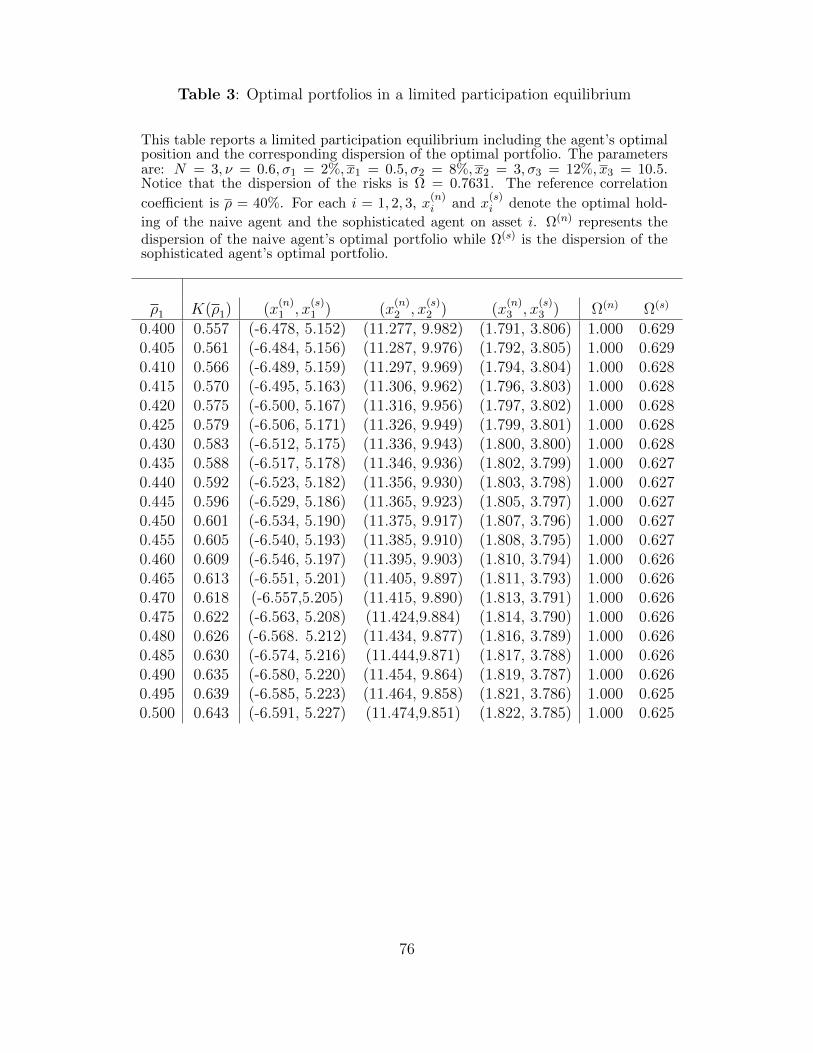
Table 3: Optimal portfolios in a limited participation equilibrium

This table reports a limited participation equilibrium including the agent’s optimalposition and the corresponding dispersion of the optimal portfolio. The parametersare: N = 3, ν = 0.6, σ1 = 2%, x1 = 0.5, σ2 = 8%, x2 = 3, σ3 = 12%, x3 = 10.5.Notice that the dispersion of the risks is Ω = 0.7631. The reference correlation

coefficient is ρ = 40%. For each i = 1, 2, 3, x(n)i and x

(s)i denote the optimal hold-

ing of the naive agent and the sophisticated agent on asset i. Ω(n) represents thedispersion of the naive agent’s optimal portfolio while Ω(s) is the dispersion of thesophisticated agent’s optimal portfolio.

ρ1 K(ρ1) (x(n)1 , x

(s)1 ) (x

(n)2 , x

(s)2 ) (x

(n)3 , x

(s)3 ) Ω(n) Ω(s)

0.400 0.557 (-6.478, 5.152) (11.277, 9.982) (1.791, 3.806) 1.000 0.6290.405 0.561 (-6.484, 5.156) (11.287, 9.976) (1.792, 3.805) 1.000 0.6290.410 0.566 (-6.489, 5.159) (11.297, 9.969) (1.794, 3.804) 1.000 0.6280.415 0.570 (-6.495, 5.163) (11.306, 9.962) (1.796, 3.803) 1.000 0.6280.420 0.575 (-6.500, 5.167) (11.316, 9.956) (1.797, 3.802) 1.000 0.6280.425 0.579 (-6.506, 5.171) (11.326, 9.949) (1.799, 3.801) 1.000 0.6280.430 0.583 (-6.512, 5.175) (11.336, 9.943) (1.800, 3.800) 1.000 0.6280.435 0.588 (-6.517, 5.178) (11.346, 9.936) (1.802, 3.799) 1.000 0.6270.440 0.592 (-6.523, 5.182) (11.356, 9.930) (1.803, 3.798) 1.000 0.6270.445 0.596 (-6.529, 5.186) (11.365, 9.923) (1.805, 3.797) 1.000 0.6270.450 0.601 (-6.534, 5.190) (11.375, 9.917) (1.807, 3.796) 1.000 0.6270.455 0.605 (-6.540, 5.193) (11.385, 9.910) (1.808, 3.795) 1.000 0.6270.460 0.609 (-6.546, 5.197) (11.395, 9.903) (1.810, 3.794) 1.000 0.6260.465 0.613 (-6.551, 5.201) (11.405, 9.897) (1.811, 3.793) 1.000 0.6260.470 0.618 (-6.557,5.205) (11.415, 9.890) (1.813, 3.791) 1.000 0.6260.475 0.622 (-6.563, 5.208) (11.424,9.884) (1.814, 3.790) 1.000 0.6260.480 0.626 (-6.568. 5.212) (11.434, 9.877) (1.816, 3.789) 1.000 0.6260.485 0.630 (-6.574, 5.216) (11.444,9.871) (1.817, 3.788) 1.000 0.6260.490 0.635 (-6.580, 5.220) (11.454, 9.864) (1.819, 3.787) 1.000 0.6260.495 0.639 (-6.585, 5.223) (11.464, 9.858) (1.821, 3.786) 1.000 0.6250.500 0.643 (-6.591, 5.227) (11.474,9.851) (1.822, 3.785) 1.000 0.625

76