cosmografi
Upload: 08-geografi-di-universitas-negeri-gorontalonext-13-geografi-di-universitas-negeri-makassar
Post on 17-Jul-2015
42 views
TRANSCRIPT

arXiv:gr-qc/0703122v3 31 Jul 2007
Cosmography: Extracting the Hubble series from
the supernova dataC´eline Catto¨en and Matt VisserSchool of Mathematics, Statistics, and Computer Science,Victoria University of Wellington, PO Box 600, Wellington, New ZealandE-mail: [email protected], [email protected] (cosmokinetics) is the part of cosmology that proceeds by makingminimal dynamic assumptions. One keeps the geometry and symmetries of FLRWspacetime, at least as a working hypothesis, but does not assume the Friedmannequations (Einstein equations), unless and until absolutely necessary. By doing soit is possible to defer questions about the equation of state of the cosmological fluid,and concentrate more directly on the observational situation. In particular, the big“picture is best brought into focus by performing a fit of all available supernova data”to the Hubble relation, from the current epoch at least back to redshift z _ 1.75.
We perform a number of inter-related cosmographic fits to the legacy05 and gold06supernova datasets. We pay particular attention to the influence of both statisticaland systematic uncertainties, and also to the extent to which the choice of distancescale and manner of representing the redshift scale affect the cosmological parameters.While the preponderance of evidence certainly suggests an accelerating universe,“ ”we would argue that (based on the supernova data) this conclusion is not currentlysupported beyond reasonable doubt . As part of the analysis we develop two“ ”particularly transparent graphical representations of the redshift-distance relation —representations in which acceleration versus deceleration reduces to the question ofwhether the graph slopes up or down.Turning to the details of the cosmographic fits, three issues in particular concern us:First, the fitted value for the deceleration parameter changes significantly depending
on whether one performs a _2 fit to the luminosity distance, proper motion distance,angular diameter distance, or other suitable distance surrogate. Second, the fitted valuefor the deceleration parameter changes significantly depending on whether one usesthe traditional redshift variable z, or what we shall argue is on theoretical grounds animproved parameterization y = z/(1+z). Third, the published estimates for systematicuncertainties are sufficiently large that they certainly impact on, and to a large extentundermine, the usual purely statistical tests of significance. We conclude that the casefor an accelerating universe is considerably less watertight than commonly believed.Based on a talk presented by Matt Visser at KADE 06, the Key approaches to Dark“Energy conference, Barcelona, August 2006; follow up at GR18, Sydney, July 2007.”Keywords: Supernova data, gold06, legacy05, Hubble law, data fitting, deceleration,jerk, snap, statistical uncertainties, systematic uncertainties, high redshift,convergence.arXiv: gr-qc/0703122; Dated: 26 March 2007;
revised 10 May 2007; revised 31 July 2007; LATEX-ed 10 February 2010.
Cosmography: Extracting the Hubble series from the supernova data 2
Comment on the revisions
•In the version 2 revision we have responded to community feedback by extending
and clarifying the discussion, and by adding numerous additional references. While
our overall conclusions remain unchanged we have rewritten our discussion of both
statistical and systematic uncertainties to use language that is more in line with

the norms adopted by the supernova community.
•In particular we have adopted the nomenclature of the NIST reference on the
“Uncertainty of Measurement Results” http://physics.nist.gov/cuu/Uncertainty/,
which is itself a distillation of NIST Technical Note 1297 “Guidelines for Evaluating
and Expressing the Uncertainty of NIST Measurement Results”, which is in turn
based on the ISO’s “Guide to the Expression of Uncertainty in Measurement”
(GUM).
•This NIST document summarizes the norms and recommendations established by
international agreement between the NIST, the ISO, the BIPM, and the CIPM.
•By closely adhering to this widely accepted standard, and to the norms adopted
by the supernova community, we hope we have now minimized the risk of
miscommunication and misunderstanding.
•We emphasize: Our overall conclusions remain unchanged. The case for an
accelerating universe is considerably less watertight than commonly believed.
– Regardless of one’s views on how to combine formal estimates of uncertainty,
the very fact that different distance scales yield data-fits with such widely
discrepant values strongly suggests the need for extreme caution in interpreting
the supernova data.
– Ultimately, it is the fact that figures 7–10 do not exhibit any overwhelmingly
obvious trend that makes it so difficult to make a robust and reliable estimate
of the sign of the deceleration parameter.
•Version 3 now adds a little more discussion and historical context. Some historical
graphs are added, plus some additional references, and a few clarifying comments.
No physics changes.
CONTENTS 3
Contents
1 Introduction 5
2 Some history 7
3 Cosmological distance scales 8

4 New versions of the Hubble law 13
5 Why is the redshift expansion badly behaved for z > 1? 15
5.1 Convergence . . . . . . . . . . . . . . . . . . . . . . . . . . . . . . . . . . 15
5.2 Pivoting . . . . . . . . . . . . . . . . . . . . . . . . . . . . . . . . . . . . 16
5.3 Other singularities . . . . . . . . . . . . . . . . . . . . . . . . . . . . . . 17
6 Improved redshift variable for the Hubble relation 18
7 More versions of the Hubble law 20
8 Supernova data 21
8.1 The legacy05 dataset . . . . . . . . . . . . . . . . . . . . . . . . . . . . . 21
8.2 The gold06 dataset . . . . . . . . . . . . . . . . . . . . . . . . . . . . . . 23
8.3 Peculiar velocities . . . . . . . . . . . . . . . . . . . . . . . . . . . . . . . 26
9 Data fitting: Statistical uncertanties 26
9.1 Finite-polynomial truncated-Taylor-series fit . . . . . . . . . . . . . . . . 26
9.2 _2 goodness of fit . . . . . . . . . . . . . . . . . . . . . . . . . . . . . . . 28
9.3 F-test of additional terms . . . . . . . . . . . . . . . . . . . . . . . . . . 28
9.4 Uncertainties in the coefficients aj and bj . . . . . . . . . . . . . . . . . . 29
9.5 Estimates of the deceleration and jerk . . . . . . . . . . . . . . . . . . . . 30
10 Model-building uncertainties 32
11 Systematic uncertainties 34
11.1 Major philosophies underlying the analysis of statistical uncertainty . . . 34
11.2 Deceleration . . . . . . . . . . . . . . . . . . . . . . . . . . . . . . . . . . 35
11.3 Jerk . . . . . . . . . . . . . . . . . . . . . . . . . . . . . . . . . . . . . . 36
12 Historical estimates of systematic uncertainty 36
12.1 Deceleration . . . . . . . . . . . . . . . . . . . . . . . . . . . . . . . . . . 37
12.2 Jerk . . . . . . . . . . . . . . . . . . . . . . . . . . . . . . . . . . . . . . 38
13 Combined uncertainties 39
14 Expanded uncertainty 40
CONTENTS 4
15 Results 41
16 Conclusions 41
Appendix A

Some ambiguities in least-squares fitting 43
Appendix B
Combining measurements from different models 47
References 48
Cosmography: Extracting the Hubble series from the supernova data 5
1. Introduction
From various observations of the Hubble relation, most recently including the supernova
data [1, 2, 3, 4, 5, 6], one is by now very accustomed to seeing many plots of luminosity
distance dL versus redshift z. But are there better ways of representing the data?
For instance, consider cosmography (cosmokinetics) which is the part of cosmology
that proceeds by making minimal dynamic assumptions. One keeps the geometry and
symmetries of FLRW spacetime,
ds2 = −c2 dt2 + a(t)2
_
dr2
1 −k r2 + r2(d_2 + sin2 _ d_2)
_
, (1)
at least as a working hypothesis, but does not assume the Friedmann equations
(Einstein
equations), unless and until absolutely necessary. By doing so it is possible to defer
questions about the equation of state of the cosmological fluid, minimize the number of
theoretical assumptions one is bringing to the table, and so concentrate more directly
on the observational situation.
In particular, the “big picture” is best brought into focus by performing a global
fit of all available supernova data to the Hubble relation, from the current epoch at
least back to redshift z _ 1.75. Indeed, all the discussion over acceleration versus

deceleration, and the presence (or absence) of jerk (and snap) ultimately boils down, in
a cosmographic setting, to doing a finite-polynomial truncated–Taylor series fit of the
distance measurements (determined by supernovae and other means) to some suitable
form of distance–redshift or distance–velocity relationship. Phrasing the question to be
investigated in this way keeps it as close as possible to Hubble’s original statement of
the problem, while minimizing the number of extraneous theoretical assumptions one is
forced to adopt. For instance, it is quite standard to phrase the investigation in terms
of the luminosity distance versus redshift relation [7, 8]:
dL(z) =c zH0_
1 +
1
2
[1 −q0] z + O(z2)
_
, (2)
and its higher-order extension [9, 10, 11, 12]
dL(z) =c zH0_
1 +
1
2
[1 −q0] z −

1
6_
1 −q0 −3q2
0 + j0 +kc2H2
0 a2
0_
z2 + O(z3)_
, (3)
A central question thus has to do with the choice of the luminosity distance as the
primary quantity of interest — there are several other notions of cosmological distance
that can be used, some of which (we shall see) lead to simpler and more tractable
versions of the Hubble relation. Furthermore, as will quickly be verified by looking at
the derivation (see, for example, [7, 8, 9, 10, 11, 12], the standard Hubble law is actually
a Taylor series expansion derived for small z, whereas much of the most interesting
recent supernova data occurs at z > 1. Should we even trust the usual formalism for
large z > 1? Two distinct things could go wrong:
•The underlying Taylor series could fail to converge.
Cosmography: Extracting the Hubble series from the supernova data 6
•Finite truncations of the Taylor series might be a bad approximation to the exact
result.
In fact, both things happen. There are good mathematical and physical reasons for this
undesirable behaviour, as we shall discuss below. We shall carefully explain just what

goes wrong — and suggest various ways of improving the situation. Our ultimate goal
will be to find suitable forms of the Hubble relation that are well adapted to performing
fits to all the available distance versus redshift data.
Moreover — once one stops to consider it carefully — why should the cosmology
community be so fixated on using the luminosity distance dL (or its logarithm,
proportional to the distance modulus) and the redshift z as the relevant parameters?
In principle, in place of luminosity distance dL(z) versus redshift z one could just
as easily plot f(dL, z) versus g(z), choosing f(dL, z) and g(z) to be arbitrary locally
invertible functions, and exactly the same physics would be encoded. Suitably choosing
the quantities to be plotted and fit will not change the physics, but it might improve
statistical properties and insight. (And we shall soon see that it will definitely improve
the behaviour of the Taylor series.)
By comparing cosmological parameters obtained using multiple different fits of
the Hubble relation to different distance scales and different parameterizations of the
redshift we can then assess the robustness and reliability of the data fitting procedure.
In performing this analysis we had hoped to verify the robustness of the Hubble
relation, and to possibly obtain improved estimates of cosmological parameters such
as the deceleration parameter and jerk parameter, thereby complementing other recent
cosmographic and cosmokinetic analyses such as [13, 14, 15, 16, 17], as well as other
analyses that take a sometimes skeptical view of the totality of the observational
data [18, 19, 20, 21, 22]. The actual results of our current cosmographic fits to the
data are considerably more ambiguous than we had initially expected, and there are
many subtle issues hiding in the simple phrase “fitting the data”.
In the following sections we first discuss the various cosmological distance scales,
and the related versions of the Hubble relation. We then discuss technical problems
with the usual redshift variable for z > 1, and how to ameliorate them, leading to
yet more versions of the Hubble relation. After discussing key features of the supernova
data, we perform, analyze, and contrast multiple fits to the Hubble relation — providing
discussions of model-building uncertainties (some technical details being relegated to
the
appendices) and sensitivity to systematic uncertainties. Finally we present our results

and conclusions: There is a disturbingly strong model-dependence in the resulting
estimates for the deceleration parameter. Furthermore, once realistic estimates of
systematic uncertainties (based on the published data) are budgeted for it becomes
clear that purely statistical estimates of goodness of fit are dangerously misleading.
While the “preponderance of evidence” certainly suggests an accelerating universe, we
would argue that this conclusion is not currently supported “beyond reasonable doubt”
— the supernova data (considered by itself) certainly suggests an accelerating
universe,
Cosmography: Extracting the Hubble series from the supernova data 7
it is not sufficient to allow us to reliably conclude that the universe is accelerating.‡
2. Some history
The need for a certain amount of caution in interpreting the observational data can
clearly be inferred from a dispassionate reading of history. We reproduce below
Hubble’s
original 1929 version of what is now called the Hubble plot (Figure 1) [23], a modern
update from 2004 (Figure 2) [24], and a very telling plot of the estimated value of the
Hubble parameter as a function of publication date (Figure 3) [24]. Regarding this last
plot, Kirshner is moved to comment [24]:
“At each epoch, the estimated error in the Hubble constant is small compared
with the subsequent changes in its value. This result is a symptom of
underestimated systematic errors.”Figure 1. Hubble s original 1929 plot [23]. Note the rather large scatter in the data.’
It is important to realise that the systematic under-estimating of systematic
uncertainties is a generic phenomenon that cuts across disciplines and sub-fields, it
is not a phenomenon that is limited to cosmology. For instance, the “Particle Data
Group” [http://pdg.lbl.gov/] in their bi-annual “Review of Particle Properties” publishes
fascinating plots of estimated values of various particle physics parameters as a
function ‡If one adds additional theoretical assumptions, such as by specifically fitting to a _-CDM model,
the situation at first glance looks somewhat better but this is then telling you as much about one s— ’choice of theoretical model as it is about the observational situation.
Cosmography: Extracting the Hubble series from the supernova data 8
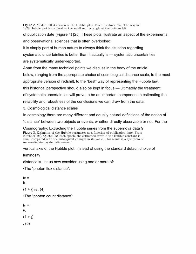
Figure 2. Modern 2004 version of the Hubble plot. From Kirshner [24]. The original1929 Hubble plot is confined to the small red rectangle at the bottom left.
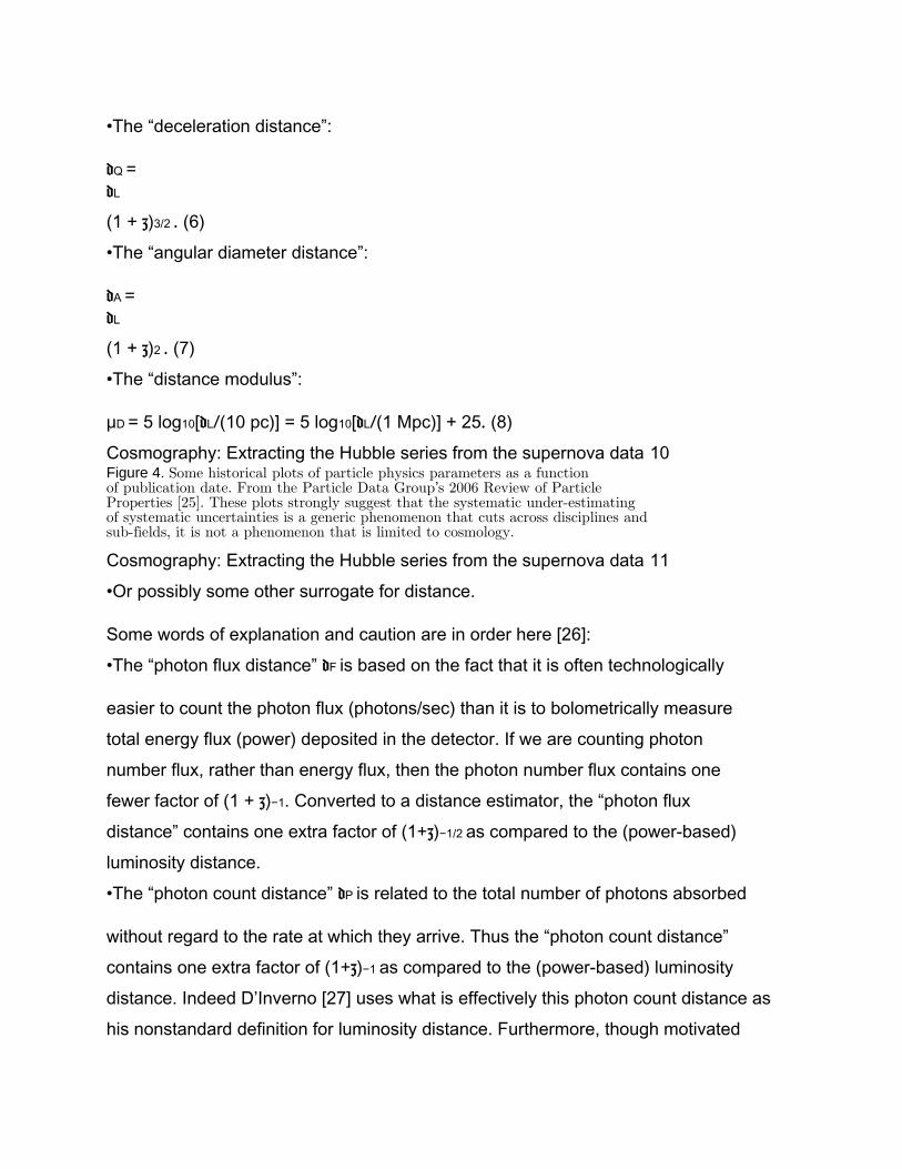
of publication date (Figure 4) [25]. These plots illustrate an aspect of the experimental
and observational sciences that is often overlooked:
It is simply part of human nature to always think the situation regarding
systematic uncertainties is better than it actually is — systematic uncertainties
are systematically under-reported.
Apart from the many technical points we discuss in the body of the article
below, ranging from the appropriate choice of cosmological distance scale, to the most
appropriate version of redshift, to the “best” way of representing the Hubble law,
this historical perspective should also be kept in focus — ultimately the treatment
of systematic uncertainties will prove to be an important component in estimating the
reliability and robustness of the conclusions we can draw from the data.
3. Cosmological distance scales
In cosmology there are many different and equally natural definitions of the notion of
“distance” between two objects or events, whether directly observable or not. For the
Cosmography: Extracting the Hubble series from the supernova data 9Figure 3. Estimates of the Hubble parameter as a function of publication date. FromKirshner [24]. Quote: At each epoch, the estimated error in the Hubble constant is“small compared with the subsequent changes in its value. This result is a symptom ofunderestimated systematic errors.”
vertical axis of the Hubble plot, instead of using the standard default choice of
luminosity
distance dL, let us now consider using one or more of:
•The “photon flux distance”:
dF =dL
(1 + z)1/2 . (4)
•The “photon count distance”:
dP =dL
(1 + z)
. (5)
•The “deceleration distance”:
dQ =dL
(1 + z)3/2 . (6)
•The “angular diameter distance”:
dA =dL
(1 + z)2 . (7)
•The “distance modulus”:
μD = 5 log10[dL/(10 pc)] = 5 log10[dL/(1 Mpc)] + 25. (8)
Cosmography: Extracting the Hubble series from the supernova data 10Figure 4. Some historical plots of particle physics parameters as a functionof publication date. From the Particle Data Group s 2006 Review of Particle’Properties [25]. These plots strongly suggest that the systematic under-estimatingof systematic uncertainties is a generic phenomenon that cuts across disciplines andsub-fields, it is not a phenomenon that is limited to cosmology.
Cosmography: Extracting the Hubble series from the supernova data 11
•Or possibly some other surrogate for distance.
Some words of explanation and caution are in order here [26]:
•The “photon flux distance” dF is based on the fact that it is often technologically
easier to count the photon flux (photons/sec) than it is to bolometrically measure
total energy flux (power) deposited in the detector. If we are counting photon
number flux, rather than energy flux, then the photon number flux contains one
fewer factor of (1 + z)−1. Converted to a distance estimator, the “photon flux
distance” contains one extra factor of (1+z)−1/2 as compared to the (power-based)
luminosity distance.
•The “photon count distance” dP is related to the total number of photons absorbed
without regard to the rate at which they arrive. Thus the “photon count distance”
contains one extra factor of (1+z)−1 as compared to the (power-based) luminosity
distance. Indeed D’Inverno [27] uses what is effectively this photon count distance as
his nonstandard definition for luminosity distance. Furthermore, though motivated

very differently, this quantity is equal to Weinberg’s definition of proper motion
distance [7], and is also equal to Peebles’ version of angular diameter distance [8].
That is:
dP = dL,D’Inverno = dproper,Weinberg = dA,Peebles. (9)
•The quantity dQ is (as far as we can tell) a previously un-named quantity that seems
to have no simple direct physical interpretation — but we shall soon see why it is
potentially useful, and why it is useful to refer to it as the “deceleration distance”.
•The quantity dA is Weinberg’s definition of angular diameter distance [7],
corresponding to the physical size of the object when the light was emitted, divided
by its current angular diameter on the sky. This differs from Peebles’ definition
of angular diameter distance [8], which corresponds to what the size of the object
would be at the current cosmological epoch if it had continued to co-move with
the cosmological expansion (that is, the “comoving size”), divided by its current
angular diameter on the sky. Weinberg’s dA exhibits the (at first sight perplexing,
but physically correct) feature that beyond a certain point dA can actually decrease
as one moves to older objects that are clearly “further” away. In contrast Peebles’
version of angular diameter distance is always increasing as one moves “further”
away. Note that
dA,Peebles = (1 + z) dA. (10)
•Finally, note that the distance modulus can be rewritten in terms of traditional
stellar magnitudes as
μD = μapparent −μabsolute. (11)
The continued use of stellar magnitudes and the distance modulus in the context
of cosmology is largely a matter of historical tradition, though we shall soon see
that the logarithmic nature of the distance modulus has interesting and useful side
Cosmography: Extracting the Hubble series from the supernova data 12
effects. Note that we prefer as much as possible to deal with natural logarithms:
ln x = ln(10) log10 x. Indeed
μD =

5
ln 10
ln[dL/(1 Mpc)] + 25, (12)
so that
ln[dL/(1 Mpc)] =
ln 10
5
[μD −25]. (13)
Obviously
dL _ dF _ dP _ dQ _ dA. (14)
Furthermore these particular distance scales satisfy the property that they converge on
each other, and converge on the naive Euclidean notion of distance, as z ! 0.
To simplify subsequent formulae, it is now useful to define the “Hubble distance” §
dH =cH0
, (15)
so that for H0 = 73 +3
−4 (km/sec)/Mpc [25] we have
dH = 4100 +240
−160 Mpc. (16)
Furthermore we choose to set
0 = 1 +kc2H2
0a2
0
= 1 +k d2
H
a2
0

. (17)
For our purposes 0 is a purely cosmographic definition without dynamical content.
(Only if one additionally invokes the Einstein equations in the form of the Friedmann
equations does 0 have the standard interpretation as the ratio of total density to the
Hubble density, but we would be prejudging things by making such an identification in
the current cosmographic framework.) In the cosmographic framework k/a2
0 is simply
the present day curvature of space (not spacetime), while d −2
H = H2
0/c2 is a measure
of the contribution of expansion to the spacetime curvature of the FLRW geometry.
More precisely, in a FRLW universe the Riemann tensor has (up to symmetry) only two
non-trivial components. In an orthonormal basis:
Rˆ_ ˆ_ˆ_ ˆ_ =k
a2 +
˙a2
c2 a2 =k
a2 +H2
c2 ; (18)
Rˆtˆrˆtˆr = −
¨ac2 a
=q H2
c2 . (19)
Then at arbitrary times can be defined purely in terms of the Riemann tensor of the
FLRW spacetime as
=

Rˆ_ ˆ_ˆ_ ˆ_( ˙a ! 0)
Rˆ_ ˆ_ˆ_ ˆ_(k ! 0)
. (20)§ The Hubble distance “ ” dH = c/H0 is sometimes called the Hubble radius , or the Hubble sphere ,“ ” “ ”
or even the speed of light sphere [SLS] [28]. Sometimes Hubble distance is used to refer to the naive“ ” “ ”estimate d = dH z coming from the linear part of the Hubble relation and ignoring all higher-orderterms this is definitely — not our intended meaning.
Cosmography: Extracting the Hubble series from the supernova data 13
4. New versions of the Hubble law
New versions of the Hubble law are easily calculated for each of these cosmological
distance scales. Explicitly:
dL(z) = dH z_
1 −
1
2
[−1 + q0] z +
1
6_
q0 + 3q2
0 −(j0 + 0)
_
z2 + O(z3)_

. (21)
dF (z) = dH z_
1 −
1
2
q0z +
1
24_
3 + 10q0 + 12q2
0 −4(j0 + 0)
_
z2 + O(z3)_
. (22)
dP (z) = dH z_
1 −
1
2
[1 + q0] z +
1
6

_
3 + 4q0 + 3q2
0 −(j0 + 0)
_
z2 + O(z3)_
. (23)
dQ(z) = dH z_
1 −
1
2
[2 + q0] z +
1
24_
27 + 22q0 + 12q2
0 −4(j0 + 0)
_
z2 + O(z3)_
. (24)
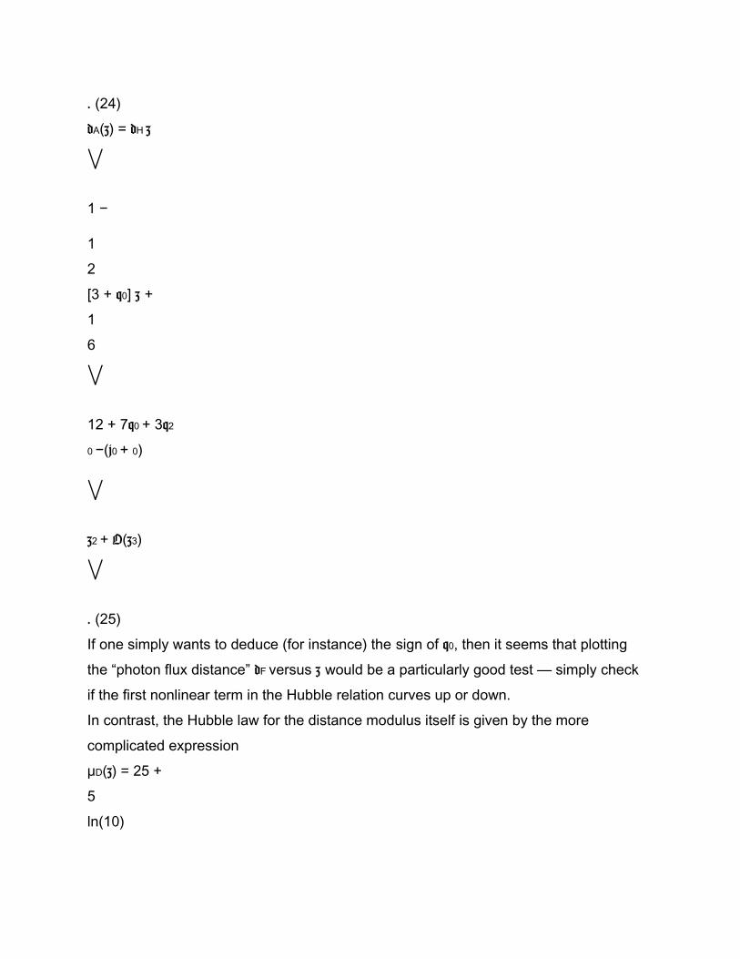
dA(z) = dH z_
1 −
1
2
[3 + q0] z +
1
6_
12 + 7q0 + 3q2
0 −(j0 + 0)
_
z2 + O(z3)_
. (25)
If one simply wants to deduce (for instance) the sign of q0, then it seems that plotting
the “photon flux distance” dF versus z would be a particularly good test — simply check
if the first nonlinear term in the Hubble relation curves up or down.
In contrast, the Hubble law for the distance modulus itself is given by the more
complicated expression
μD(z) = 25 +
5
ln(10)

_
ln(dH/Mpc) + ln z
+
1
2
[1 −q0] z −
1
24_
3 −10q0 −9q2
0 + 4(j0 + 0)_
z2 + O(z3)_
. (26)
However, when plotting μD versus z, most of the observed curvature in the plot comes
from the universal (ln z) term, and so carries no real information and is relatively
uninteresting. It is much better to rearrange the above as:
ln[dL/(z Mpc)] =
ln 10
5
[μD −25] −ln z
= ln(dH/Mpc)−
1

2
[−1 + q0] z +
1
24_
−3 + 10q0 + 9q2
0 −4(j0 + 0)
_
z2 + O(z3). (27)
In a similar manner one has
ln[dF /(z Mpc)] =
ln 10
5
[μD −25] −ln z −
1
2
ln(1 + z)
= ln(dH/Mpc)−
1
2
q0z +
1
24_
3 + 10q0 + 9q2

0 −4(j0 + 0)
_
z2 + O(z3). (28)
Cosmography: Extracting the Hubble series from the supernova data 14
ln[dP /(z Mpc)] =
ln 10
5
[μD −25] −ln z −ln(1 + z)
= ln(dH/Mpc)−
1
2
[1 + q0] z +
1
24_
9 + 10q0 + 9q2
0 −4(j0 + 0)
_
z2 + O(z3). (29)
ln[dQ/(z Mpc)] =
ln 10
5
[μD −25] −ln z −
3
2

ln(1 + z)
= ln(dH/Mpc)−
1
2
[2 + q0] z +
1
24_
15 + 10q0 + 9q2
0 −4(j0 + 0)
_
z2 + O(z3). (30)
ln[dA/(z Mpc)] =
ln 10
5
[μD −25] −ln z −2 ln(1 + z)
= ln(dH/Mpc)−
1
2
[3 + q0] z +
1
24_
21 + 10q0 + 9q2

0 −4(j0 + 0)
_
z2 + O(z3). (31)
These logarithmic versions of the Hubble law have several advantages — fits to these
relations are easily calculated in terms of the observationally reported distance moduli
μD and their estimated statistical uncertainties [1, 2, 3, 4, 5]. (Specifically there is no
need to transform the statistical uncertainties on the distance moduli beyond a universal
multiplication by the factor [ln 10]/5.) Furthermore the deceleration parameter q0 is easy
to extract as it has been “untangled” from both Hubble parameter and the combination
(j0 + 0).
Note that it is always the combination (j0 + 0) that arises in these third-order
Hubble relations, and that it is even in principle impossible to separately determine j0
and 0 in a cosmographic framework. The reason for this degeneracy is (or should be)
well-known [7, p. 451]: Consider the exact expression for the luminosity distance in any
FLRW universe, which is usually presented in the form [7, 8]
dL(z) = a0 (1 + z) sink_
cH0 a0
Z z
0
H0
H(z)
dz_
, (32)
where

sink(x) =8><
>:
sin(x), k = +1;
x, k = 0;
sinh(x), k = −1.
(33)
By inspection, even if one knows H(z) exactly for all z one cannot determine dL(z)
without independent knowledge of k and a0. Conversely even if one knows dL(z) exactly
for all z one cannot determine H(z) without independent knowledge of k and a0. Indeed
let us rewrite this exact result in a slightly different fashion as
dL(z) = a0 (1 + z)
sin(pk dH
a0
Z z
0
H0
H(z)
dz)
pk
, (34)
Cosmography: Extracting the Hubble series from the supernova data 15
where this result now holds for all k provided we interpret the k = 0 case in the obvious

limiting fashion. Equivalently, using the cosmographic 0 as defined above we have the
exact cosmographic result that for all 0:
dL(z) = dH (1 + z)
sin_
p0 −1
Z z
0
H0
H(z)
dz_
p0 −1
. (35)
This form of the exact Hubble relation makes it clear that an independent determination
of 0 (equivalently, k/a2
0 ), is needed to complete the link between a(t) and dL(z). When
Taylor expanded in terms of z, this expression leads to a degeneracy at third-order,
which is where 0 [equivalently k/a2
0 ] first enters into the Hubble series [11, 12].
What message should we take from this discussion? There are many physically
equivalent versions of the Hubble law, corresponding to many slightly different
physically
reasonable definitions of distance, and whether we choose to present the Hubble law
linearly or logarithmically. If one were to have arbitrarily small scatter/error bars on
the observational data, then the choice of which Hubble law one chooses to fit to would
not matter. In the presence of significant scatter/uncertainty there is a risk that the fit

might depend strongly on the choice of Hubble law one chooses to work with. (And if
the resulting values of the deceleration parameter one obtains do depend significantly
on which distance scale one uses, this is evidence that one should be very cautious
in interpreting the results.) Note that the two versions of the Hubble law based on
“photon flux distance” dF stand out in terms of making the deceleration parameter
easy to visualize and extract.
5. Why is the redshift expansion badly behaved for z > 1?
In addition to the question of which distance measure one chooses to use, there is a
basic and fundamental physical and mathematical reason why the traditional redshift
expansion breaks down for z > 1.
5.1. Convergence
Consider the exact Hubble relation (32). This is certainly nicely behaved, and
possesses
no obvious poles or singularities, (except possibly at a turnaround event where H(z) !
0, more on this below). However if we attempt to develop a Taylor series expansion in
redshift z, using what amounts to the definition of the Hubble H0, deceleration q0, and
jerk j0 parameters, then:
1
1 + z
=
a(t)a0
= 1 + H0 (t −t0) −
q0 H2
0
2!
(t −t0)2 +
j0 H3
0
3!
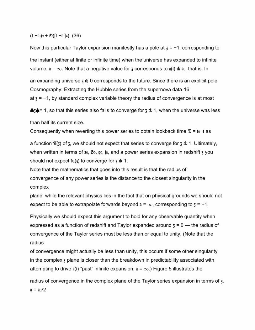
(t −t0)3 + O([t −t0]4). (36)
Now this particular Taylor expansion manifestly has a pole at z = −1, corresponding to
the instant (either at finite or infinite time) when the universe has expanded to infinite
volume, a = 1. Note that a negative value for z corresponds to a(t) > a0, that is: In
an expanding universe z < 0 corresponds to the future. Since there is an explicit pole
Cosmography: Extracting the Hubble series from the supernova data 16
at z = −1, by standard complex variable theory the radius of convergence is at most
|z| = 1, so that this series also fails to converge for z > 1, when the universe was less
than half its current size.
Consequently when reverting this power series to obtain lookback time T = t0−t as
a function T(z) of z, we should not expect that series to converge for z > 1. Ultimately,
when written in terms of a0, H0, q0, j0, and a power series expansion in redshift z you
should not expect dL(z) to converge for z > 1.
Note that the mathematics that goes into this result is that the radius of
convergence of any power series is the distance to the closest singularity in the
complex
plane, while the relevant physics lies in the fact that on physical grounds we should not
expect to be able to extrapolate forwards beyond a = 1, corresponding to z = −1.
Physically we should expect this argument to hold for any observable quantity when
expressed as a function of redshift and Taylor expanded around z = 0 — the radius of
convergence of the Taylor series must be less than or equal to unity. (Note that the
radius
of convergence might actually be less than unity, this occurs if some other singularity
in the complex z plane is closer than the breakdown in predictability associated with
attempting to drive a(t) “past” infinite expansion, a = 1.) Figure 5 illustrates the
radius of convergence in the complex plane of the Taylor series expansion in terms of z.
a = a0/2

Complex z plane
z = 0
a = a0
radius of convergence
z = −1
a = +1
z = 1 z = +1
a = 0Figure 5. Qualitative sketch of the behaviour of the scale factor a and the radius ofconvergence of the Taylor series in z-redshift.
Consequently, we must conclude that observational data regarding dL(z) for z > 1
is not going to be particularly useful in fitting a0, H0, q0, and j0, to the usual traditional
version of the Hubble relation.
5.2. Pivoting
A trick that is sometimes used to improve the behaviour of the Hubble law is to Taylor
expand around some nonzero value of z, which might be called the “pivot”. That is, we
take
z = zpivot + _z, (37)
Cosmography: Extracting the Hubble series from the supernova data 17
and expand in powers of _z. If we choose to do so, then observe
1
1 + zpivot + _z
= 1+H0 (t−t0)−
1
2q0 H2
0 (t−t0)2+
1
3!j0 H3

0 (t−t0)3+O([t−t0]4). (38)
The pole is now located at:
_z = −(1 + zpivot), (39)
which again physically corresponds to a universe that has undergone infinite expansion,
a = 1. The radius of convergence is now
|_z| _ (1 + zpivot), (40)
and we expect the pivoted version of the Hubble law to fail for
z > 1 + 2 zpivot. (41)
So pivoting is certainly helpful, and can in principle extend the convergent region of the
Taylor expanded Hubble relation to somewhat higher values of z, but maybe we can do
even better?
5.3. Other singularities
Other singularities that might further restrict the radius of convergence of the Taylor
expanded Hubble law (or any other Taylor expanded physical observable) are also
important. Chief among them are the singularities (in the Taylor expansion) induced
by turnaround events. If the universe has a minimum scale factor amin (corresponding
to a “bounce”) then clearly it is meaningless to expand beyond
1 + zmax = a0/amin; zmax = a0/amin −1; (42)
implying that we should restrict our attention to the region
|z| < zmax = a0/amin −1. (43)
Since for other reasons we had already decided we should restrict attention to |z| < 1,
and since on observational grounds we certainly expect any “bounce”, if it occurs at all,
to occur for zmax _ 1, this condition provides no new information.
On the other hand, if the universe has a moment of maximum expansion, and then
begins to recollapse, then it is meaningless to extrapolate beyond
1 + zmin = a0/amax; zmin = −[1 −a0/amax]; (44)
implying that we should restrict our attention to the region
|z| < 1 −a0/amax. (45)
This relation now does provide us with additional constraint, though (compared to the
|z| < 1 condition) the bound is not appreciably tighter unless we are “close” to a point
of maximum expansion. Other singularities could lead to additional constraints.
Cosmography: Extracting the Hubble series from the supernova data 18
6. Improved redshift variable for the Hubble relation
Now it must be admitted that the traditional redshift has a particularly simple physical
interpretation:
1 + z =_0
_e
=
a(t0)
a(te)
, (46)
so that
z =_0 −_e
_e
=
___e
. (47)
That is, z is the change in wavelength divided by the emitted wavelength. This is
certainly simple, but there’s at least one other equally simple choice. Why not use:
y =_0 −_e
_0
=
___0

? (48)
That is, define y to be the change in wavelength divided by the observed wavelength.
This implies
1 −y =
_e
_0
=
a(te)
a(t0)
=
1
1 + z
. (49)
Now similar expansion variables have certainly been considered before. (See, for
example, Chevalier and Polarski [29], who effectively worked with the dimensionless
quantity b = a(t)/a0, so that y = 1 −b. Similar ideas have also appeared in several
related works [30, 31, 32, 33]. Note that these authors have typically been interested
in parameterizing the so-called w-parameter, rather than specifically addressing the
Hubble relation.)
Indeed, the variable y introduced above has some very nice properties:
y =z
1 + z
; z =y
1 −y
. (50)
In the past (of an expanding universe)
z 2 (0,1); y 2 (0, 1); (51)
while in the future
z 2 (−1, 0); y 2 ( 1− , 0). (52)
So the variable y is both easy to compute, and when extrapolating back to the Big Bang
has a nice finite range (0, 1). We will refer to this variable as the y-redshift. (Originally
when developing these ideas we had intended to use the variable y to develop
orthogonal
polynomial expansions on the finite interval y 2 [0, 1]. This is certainly possible, but
we shall soon see that given the current data, this is somewhat overkill, and simple
polynomial fits in y are adequate for our purposes.)
In terms of the variable y it is easy to extract a new version of the Hubble law by
simple substitution:
dL(y) = dH y_
1 −
1
2
[−3 + q0] y +
1
6_
12 −5q0 + 3q2
0 −(j0 + 0)
_
y2 + O(y3)_

. (53)
Cosmography: Extracting the Hubble series from the supernova data 19
This still looks rather messy, in fact as messy as before — one might justifiably ask in
what sense is this new variable any real improvement?
First, when expanded in terms of y, the formal radius of convergence covers much
more of the physically interesting region. Consider:
1 −y = 1 + H0 (t −t0) −
1
2q0 H2
0 (t −t0)2 +
1
3!j0 H3
0 (t −t0)3 + O([t −t0]4). (54)
This expression now has no poles, so upon reversion of the series lookback time T = t0−t
should be well behaved as a function T(y) of y — at least all the way back to the Big
Bang. (We now expect, on physical grounds, that the power series is likely to break
down if one tries to extrapolate backwards through the Big Bang.) Based on this, we
now expect dL(y), as long as it is expressed as a Taylor series in the variable y, to be a
well-behaved power series all the way to the Big Bang. In fact, since
y = +1 , Big Bang, (55)
we expect the radius of convergence to be given by |y| = 1, so that the series
converges
for
|y| < 1. (56)
Consequently, when looking into the future, in terms of the variable y we expect to

encounter problems at y = −1, when the universe has expanded to twice its current
size. Figure 6 illustrates the radius of convergence in the complex plane of the Taylor
series expansion in terms of y.
a = +1
radius of convergence
Complex y plane
y = −1 y = 0 y = 1
a = 2a0 a = a0 a = 0
y = 1−
Figure 6. Qualitative sketch of the behaviour of the scale factor a and the radius ofconvergence of the Taylor series in y-redshift.
Note the tradeoff here — z is a useful expansion parameter for arbitrarily large
universes, but breaks down for a universe half its current size or less; in contrast y is
a useful expansion parameter all the way back to the Big Bang, but breaks down for
a universe double its current size or more. Whether or not y is more suitable than z
depends very much on what you are interested in doing. This is illustrated in Figures 5
and 6. For the purposes of this article we are interested in high-redshift supernovae —
Cosmography: Extracting the Hubble series from the supernova data 20
and we want to probe rather early times — so it is definitely y that is more appropriate
here. Indeed the furthest supernova for which we presently have both spectroscopic
data
and an estimate of the distance occurs at z = 1.755 [4], corresponding to y = 0.6370.
Furthermore, using the variable y it is easier to plot very large redshift datapoints.
For example, (though we shall not pursue this point in this article), the Cosmological
Microwave Background is located at zCMB = 1088, which corresponds to yCMB = 0.999.
This point is not “out of range” as it would be if one uses the variable z.
7. More versions of the Hubble law
In terms of this new redshift variable, the “linear in distance” Hubble relations are:
dL(y) = dH y

_
1 −
1
2
[−3 + q0] y +
1
6_
12 −5q0 + 3q2
0 −(j0 + 0)
_
y2 + O(y3)_
. (57)
dF (y) = dH y_
1 −
1
2
[−2 + q0] y +
1
24
_
27 −14q0 + 12q2
0 −4(j0 + 0)
_
y2 + O(y3)_
. (58)
dP (y) = dH y_
1 −
1
2
[−1 + q0] y +
1
6_
3 −2q0 + 3q2
0 −(j0 + 0)
_
y2 + O(y3)

_
. (59)
dQ(y) = dH y_
1 −
q0
2
y +
1
12_
3 −2q0 + 12q2
0 −4(j0 + 0)
_
y2 + O(y3)_
. (60)
dA(y) = dH y_
1 −
1
2
[1 + q0] y +
1
6_
q0 + 3q2
0 −(j0 + 0)
_
y2 + O(y3)_
. (61)
Note that in terms of the y variable it is the “deceleration distance” dQ that has the
deceleration parameter q0 appearing in the simplest manner. Similarly, the “logarithmic
in distance” Hubble relations are:
ln[dL/(y Mpc)] =
ln 10
5
[μD −25] −ln y
= ln(dH/Mpc)−
1
2
[−3 + q0] y +
1
24_

21 −2q0 + 9q2
0 −4(j0 + 0)
_
y2 + O(y3). (62)
ln[dF /(y Mpc)] =
ln 10
5
[μD −25] −ln y +
1
2
ln(1 −y)
= ln(dH/Mpc)−
1
2
[−2 + q0] y +
1
24_
15 −2q0 + 9q2
0 −4(j0 + 0)
_
y2 + O(y3). (63)
Cosmography: Extracting the Hubble series from the supernova data 21
ln[dP /(y Mpc)] =
ln 10
5
[μD −25] −ln y + ln(1 −y)
= ln(dH/Mpc)−
1
2
[−1 + q0] y +
1
24_
9 −2q0 + 9q2
0 −4(j0 + 0)
_
y2 + O(y3). (64)
ln[dQ/(y Mpc)] =
ln 10
5
[μD −25] −ln y +
3
2
ln(1 −y)
= ln(dH/Mpc)−
1

2
q0 y +
1
24_
3 −2q0 + 9q2
0 −4(j0 + 0)
_
y2 + O(y3). (65)
ln[dA/(y Mpc)] =
ln 10
5
[μD −25] −ln y + 2 ln(1 −y)
= ln(dH/Mpc)−
1
2
[1 + q0] y +
1
24_
−3 −2q0 + 9q2
0 −4(j0 + 0)
_

y2 + O(y3). (66)
Again note that the “logarithmic in distance” versions of the Hubble law are attractive in
terms of maximizing the disentangling between Hubble distance, deceleration
parameter,
and jerk. Now having a selection of Hubble laws on hand, we can start to confront the
observational data to see what it is capable of telling us.
8. Supernova data
For the plots below we have used data from the supernova legacy survey (legacy05) [1,
2]
and the Riess et. al. “gold” dataset of 2006 (gold06) [4].
8.1. The legacy05 dataset
The data is available in published form [1], and in a slightly different format, via
internet [2]. (The differences amount to minor matters of choice in the presentation.)
The final processed result reported for each 115 of the supernovae is a redshift z, a
luminosity modulus μB, and an uncertainty in the luminosity modulus. The luminosity
modulus can be converted into a luminosity distance via the formula
dL = (1 Megaparsec) ×10( μB+μoffset−25)/5. (67)
The reason for the “offset” is that supernovae by themselves only determine the shape
of the Hubble relation (i.e., q0, j0, etc.), but not its absolute slope (i.e., H0) — this is
ultimately due to the fact that we do not have good control of the absolute luminosity of
the supernovae in question. The offset μoffset can be chosen to match the known value of
H0 coming from other sources. (In fact the data reported in the published article [1] has
already been normalized in this way to the “standard value” H70 = 70 (km/sec)/Mpc,
Cosmography: Extracting the Hubble series from the supernova data 22
corresponding to Hubble distance d70 = c/H70 = 4283 Mpc, whereas the data available
on the website [2] has not been normalized in this way — which is why μB as reported
on the website is systematically 19.308 stellar magnitudes smaller than that in the
published article.)
The other item one should be aware of concerns the error bars: The error bars
reported in the published article [1] are photometric uncertainties only — there is an

additional source of error to do with the intrinsic variability of the supernovae. In fact,
if you take the photometric error bars seriously as estimates of the total uncertainty,
you would have to reject the hypothesis that we live in a standard FLRW universe.
Instead, intrinsic variability in the supernovae is by far the most widely accepted
interpetation. Basically one uses the “nearby” dataset to estimate an intrinsic variability
that makes chi-squared look reasonable. This intrinsic variability of 0.13104 stellar
magnitudes [2, 13]) has been estimated by looking at low redshift supernovae (where
we
have good measures of absolute distance from other techniques), and has been
included
in the error bars reported on the website [2]. Indeed
(uncertainty)website =q
(intrinsic variability)2 + (uncertainty)2
article. (68)
With these key features of the supernovae data kept in mind, conversion to luminosity
distance and estimation of scientifically reasonable error bars (suitable for chi-square
analysis) is straightforward.0 0.1 0.2 0.3 0.4 0.5 0.6 0.7−0.8−0.7−0.6−0.5−0.4−0.3−0.2−0.100.10.2Logarithmic Deceleration distance versus y−redshift using legacy05y−redshiftln(dQ/redshift)
Figure 7. The normalized logarithm of the deceleration distance, ln(dQ/[y Mpc]), asa function of the y-redshift using the legacy05 dataset [1, 2].
To orient oneself, figure 7 focuses on the deceleration distance dQ(y), and plots
ln(dQ/[y Mpc]) versus y. Visually, the curve appears close to flat, at least out to y _ 0.4,
Cosmography: Extracting the Hubble series from the supernova data 230 0.2 0.4 0.6 0.8 1 1.2 1.4−0.8−0.7

−0.6−0.5−0.4−0.3−0.2−0.100.10.2Logarithmic Photon flux distance versus z−redshift using legacy05z−redshiftln(dF/redshift)
Figure 8. The normalized logarithm of the photon flux distance, ln(dF /[z Mpc]), asa function of the z-redshift using the legacy05 dataset [1, 2].
which is an unexpected oddity that merits further investigation—since it seems to imply
an “eyeball estimate” that q0 _ 0. Note that this is not a plot of “statistical residuals”
obtained after curve fitting — rather this can be interpreted as a plot of “theoretical
residuals”, obtained by first splitting off the linear part of the Hubble law (which is now
encoded in the intercept with the vertical axis), and secondly choosing the quantity to
be plotted so as to make the slope of the curve at zero particularly easy to interpret in
terms of the deceleration parameter. The fact that there is considerable “scatter” in the
plot should not be thought of as an artifact due to a “bad” choice of variables — instead
this choice of variables should be thought of as “good” in the sense that they provide
an honest basis for dispassionately assessing the quality of the data that currently goes
into determining the deceleration parameter. Similarly, figure 8 focuses on the photon
flux distance dF (z), and plots ln(dF /[z Mpc]) versus z. Visually, this curve is again very
close to flat, at least out to z _ 0.4. This again gives one a feel for just how tricky it is
to reliably estimate the deceleration parameter q0 from the data.
8.2. The gold06 dataset
Our second collection of data is the gold06 dataset [4]. This dataset contains 206
supernovae (including most but not all of the legacy05 supernovae) and reaches out
considerably further in redshift, with one outlier at z = 1.755, corresponding to
y = 0.6370. Though the dataset is considerably more extensive it is unfortunately
heterogeneous — combining observations from five different observing platforms over
Cosmography: Extracting the Hubble series from the supernova data 24
almost a decade. In some cases full data on the operating characteristics of the
telescopes
used does not appear to be publicly available. The issue of data inhomogeneity has
been
specifically addressed by Nesseris and Perivolaropoulos in [34]. (For related discussion,
see also [20].) In the gold06 dataset one is presented with distance moduli and total
uncertainty estimates, in particular, including the intrinsic dispersion.
A particular point of interest is that the HST-based high-z supernovae previously
published in the gold04 dataset [3] have their estimated distances reduced by
approximately 5% (corresponding to _μD = 0.10), due to a better understanding of
nonlinearities in the photodetectors. k Furthermore, the authors of [4] incorporate
(most of) the supernovae in the legacy dataset [1, 2], but do so in a modified manner
by reducing their estimated distance moduli by _μD = 0.19 (corresponding naively
to a 9.1% reduction in luminosity distance) — however this is only a change in the
normalization used in reporting the data, not a physical change in distance. Based on
revised modelling of the light curves, and ignoring the question of overall normalization,
the overlap between the gold06 and legacy05 datasets is argued to be consistent to
within
0.5% [4].
The critical point is this: Since one is still seeing _ 5% variations in estimated
supernova distances on a two-year timescale, this strongly suggests that the
unmodelled
systematic uncertainties (the so-called “unknown unknowns”) are not yet fully under
control in even the most recent data. It would be prudent to retain a systematic
uncertainty budget of at least 5% (more specifically, _μD = 0.10), and not to place too
much credence in any result that is not robust under possible systematic recalibrations
of this magnitude. Indeed the authors of [4] state:
•“... we adopt a limit on redshift-dependent systematics to be 5% per _z = 1”;
•“At present, none of the known, well-studied sources of systematic error rivals the
statistical errors presented here.”
We shall have more to say about possible systematic uncertainties, both “known
unknowns” and “unknown unknowns” later in this article.
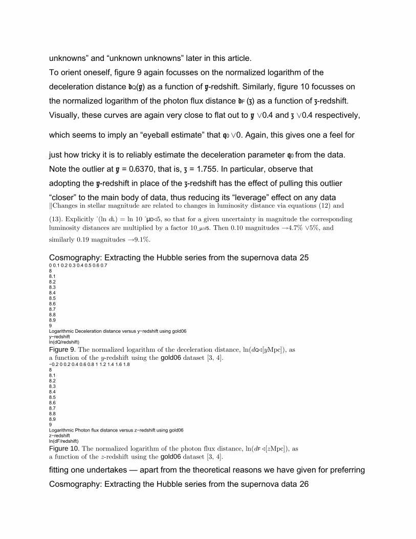
To orient oneself, figure 9 again focusses on the normalized logarithm of the
deceleration distance dQ(y) as a function of y-redshift. Similarly, figure 10 focusses on
the normalized logarithm of the photon flux distance dF (z) as a function of z-redshift.
Visually, these curves are again very close to flat out to y _ 0.4 and z _ 0.4 respectively,
which seems to imply an “eyeball estimate” that q0 _ 0. Again, this gives one a feel for
just how tricky it is to reliably estimate the deceleration parameter q0 from the data.
Note the outlier at y = 0.6370, that is, z = 1.755. In particular, observe that
adopting the y-redshift in place of the z-redshift has the effect of pulling this outlier
“closer” to the main body of data, thus reducing its “leverage” effect on any datak Changes in stellar magnitude are related to changes in luminosity distance via equations (12) and
(13). Explicitly _(ln dL) = ln 10 _μD/5, so that for a given uncertainty in magnitude the corresponding
luminosity distances are multiplied by a factor 10_μD/5. Then 0.10 magnitudes ! 4.7% _ 5%, and
similarly 0.19 magnitudes ! 9.1%.
Cosmography: Extracting the Hubble series from the supernova data 250 0.1 0.2 0.3 0.4 0.5 0.6 0.788.18.28.38.48.58.68.78.88.99Logarithmic Deceleration distance versus y−redshift using gold06y−redshiftln(dQ/redshift)
Figure 9. The normalized logarithm of the deceleration distance, ln(dQ/[y Mpc]), asa function of the y-redshift using the gold06 dataset [3, 4].−0.2 0 0.2 0.4 0.6 0.8 1 1.2 1.4 1.6 1.888.18.28.38.48.58.68.78.88.99Logarithmic Photon flux distance versus z−redshift using gold06z−redshiftln(dF/redshift)
Figure 10. The normalized logarithm of the photon flux distance, ln(dF /[z Mpc]), asa function of the z-redshift using the gold06 dataset [3, 4].
fitting one undertakes — apart from the theoretical reasons we have given for preferring
Cosmography: Extracting the Hubble series from the supernova data 26

the y-redshift, (improved convergence behaviour for the Taylor series), the fact that it
automatically reduces the leverage of high redshift outliers is a feature that is
considered
highly desirable purely for statistical reasons. In particular, the method of least-squares
is known to be non-robust with respect to outliers. One could implement more robust
regression algorithms, but they are not as easy and fast as the classical least-squares
method. We have also implemented least-squares regression against a reduced dataset
where we have trimmed out the most egregious high-z outlier, and also eliminated the
so-called “Hubble bubble” for z < 0.0233 [35, 36]. While the precise numerical values of
our estimates for the cosmological parameters then change, there is no great qualitative
change to the points we wish to make in this article, nor to the conclusions we will draw.
8.3. Peculiar velocities
One point that should be noted for both the legacy05 and gold06 datasets is the way
that peculiar velocities have been treated. While peculiar velocities would physically
seem to be best represented by assigning an uncertainty to the measured redshift, in
both these datasets the peculiar velocities have instead been modelled as some
particular
function of z-redshift and then lumped into the reported uncertainties in the distance
modulus. Working with the y-redshift ab initio might lead one to re-assess the model
for the uncertainty due to peculiar velocities. We expect such effects to be small and
have not considered them in detail.
9. Data fitting: Statistical uncertanties
We shall now compare and contrast the results of multiple least-squares fits
to the different notions of cosmological distance, using the two distinct redshift
parameterizations discussed above. Specifically, we use a finite-polynomial truncated
Taylor series as our model, and perform classical least-squares fits. This is effectively
a test of the robustness of the data-fitting procedure, testing it for model dependence.
For general background information see [37, 38, 39, 40, 41, 42, 43].
9.1. Finite-polynomial truncated-Taylor-series fit
Working (for purposes of the presentation) in terms of y-redshift, the various distance
scales can be fitted to finite-length power-series polynomials d(y) of the form

P(y) : d(y) =Xn
j=0
aj yj , (69)
where the coefficients aj all have the dimensions of distance. In contrast, logarithmic
fits are of the form
P(y) : ln[d(y)/(y Mpc)] =Xn
j=0
bj yj, (70)
Cosmography: Extracting the Hubble series from the supernova data 27
where the coefficients bj are now all dimensionless. By fitting to finite polynomials we
are implicitly making the assumption that the higher-order coefficients are all exactly
zero — this does then implicitly enforce assumptions regarding the higher-order time
derivatives dma/dtm for m > n, but there is no way to avoid making at least some
assumptions of this type [37, 38, 39, 40, 41, 42, 43].
The method of least squares requires that we minimize
_2 =XN
I=1_
PI −P(yI)
_I
_2
, (71)

where the N data points (yI , PI) represent the relevant function PI = f(μD,I , yI) of
the distance modulus μD,I at corresponding y-redshift yI , as inferred from some specific
supernovae dataset. Furthermore P(yI) is the finite polynomial model evaluated at
yI . The _I are the total statistical uncertainty in PI (including, in particular, intrinsic
dispersion). The location of the minimum value of _2 can be determined by setting the
derivatives of _2 with respect to each of the coefficients aj or bj equal to zero.
Note that the theoretical justification for using least squares assumes that the
statistical uncertainties are normally distributed Gaussian uncertainties — and there
is no real justification for this assumption in the actual data. Furthermore if the
data is processed by using some nonlinear transformation, then in general Gaussian
uncertainties will not remain Gaussian — and so even if the untransformed uncertainties
are Gaussian the theoretical justification for using least squares is again undermined
unless the scatter/uncertainties are small, [in the sense that _ _ f00(x)/f0(x)], in which
case one can appeal to a local linearization of the nonlinear data transformation f(x)
to deduce approximately Gaussian uncertainties [37, 38, 39, 40, 41, 42, 43]. As we
have
already seen, in figures 7–10, there is again no real justification for this “small scatter”
assumption in the actual data — nevertheless, in the absence of any clearly better
datafitting
prescription, least squares is the standard way of proceeding. More statistically
sophisticated techniques, such as “robust regression”, have their own distinct
drawbacks
and, even with weak theoretical underpinning, _2 data-fitting is still typically the
technique of choice [37, 38, 39, 40, 41, 42, 43].
We have performed least squares analyses, both linear in distance and logarithmic
in distance, for all of the distance scales discussed above, dL, dF , dP , dQ, and dA, both
in terms of z-redshift and y-redshift, for finite polynomials from n = 1 (linear) to n = 7
(septic). We stopped at n = 7 since beyond that point the least squares algorithm
was found to become numerically unstable due to the need to invert a numerically
illconditioned

matrix — this ill-conditioning is actually a well-known feature of high-order
least-squares polynomial fitting. We carried out the analysis to such high order purely
as a diagnostic — we shall soon see that the “most reasonable” fits are actually rather
low order n = 2 quadratic fits.
Cosmography: Extracting the Hubble series from the supernova data 28
9.2. _2 goodness of fit
A convenient measure of the goodness of fit is given by the reduced chi-square:_2
_ =_2
_
, (72)
where the factor _ = N −n −1 is the number of degrees of freedom left after fitting N
data points to the n+1 parameters. If the fitting function is a good approximation to the
parent function, then the value of the reduced chi-square should be approximately unity_2
_ _ 1. If the fitting function is not appropriate for describing the data, the value of _2
_
will be greater than 1. Also, “too good” a chi-square fit (_2
_ < 1) can come from overestimating
the statistical measurement uncertainties. Again, the theoretical justification
for this test relies on the fact that one is assuming, without a strong empirical basis,
Gaussian uncertainties [37, 38, 39, 40, 41, 42, 43]. In all the cases we considered, for
polynomials of order n = 2 and above, we found that _2
_ _ 1 for the legacy05 dataset,
and _2
_ _ 0.8 < 1 for the gold06 dataset. Linear n = 1 fits often gave high values for
_2
_ . We deduce that:
•It is desirable to keep at least quadratic n = 2 terms in all data fits.
•Caution is required when interpreting the reported statistical uncertainties in the
gold06 dataset.
(In particular, note that some of the estimates of the statistical uncertainties reported in
gold06 have themselves been determined through statistical reasoning — essentially by
adjusting _2
_ to be “reasonable”. The effects of such pre-processing become particularly
difficult to untangle when one is dealing with a heterogeneous dataset.)
9.3. F-test of additional terms
How many polynomial terms do we need to include to obtain a good approximation to
the parent function?
The difference between two _2 statistics is also distributed as _2. In particular, if
we fit a set of data with a fitting polynomial of n −1 parameters, the resulting value
of chi-square associated with the deviations about the regression _2(n −1) has N −n
degrees of freedom. If we add another term to the fitting polynomial, the corresponding
value of chi-square _2(n) has N −n −1 degrees of freedom. The difference between
these two follows the _2 distribution with one degree of freedom.
The F_ statistic follows a F distribution with _1 = 1 and _2 = N −n −1,
F_ =
_2(n −1) −_2(n)
_2(n)/(N −n −1)
. (73)
This ratio is a measure of how much the additional term has improved the value of the
reduced chi-square. F_ should be small when the function with n coefficients does not
significantly improve the fit over the polynomial fit with n −1 terms.
In all the cases we considered, the F_ statistic was not significant when one
proceeded beyond n = 2. We deduce that:
Cosmography: Extracting the Hubble series from the supernova data 29
•It is statistically meaningless to go beyond n = 2 terms in the data fits.
•This means that one can at best hope to estimate the deceleration parameter and
the jerk (or more precisely the combination j0 + 0). There is no meaningful hope
of estimating the snap parameter from the current data.
9.4. Uncertainties in the coefficients aj and bj
From the fit one can determine the standard deviations _aj and _bj for the uncertainty
of the polynomial coefficients aj or bj . It is the root sum square of the products of the
standard deviation of each data point _i, multiplied by the effect that the data point
has on the determination of the coefficient aj [37]:_2
aj =X
I"
_2
I_
@aj
@PI
_2
#
. (74)
Similarly the covariance matrix between the estimates of the coefficients in the
polynomial fit is_2
ajak =

X
I_
_2
I_
@aj
@PI__
@ak
@PI__
. (75)
Practically, the _aj and covariance matrix _2
ajak are determined as follows [37]:
•Determine the so-called curvature matrix _ for our specific polynomial model, where
the coefficients are given by
_jk =X
I_
1_2
I
(yI)j (yI)k
_
. (76)
•Invert the symmetric matrix _ to obtain the so-called error matrix _:
_ = _−1. (77)
•The uncertainty and covariance in the coefficients aj is characterized by:
_2
aj = _jj ; _2
ajak = _jk. (78)
•Finally, for any function f(ai) of the coefficients ai:
_f =sX
j,k
_2
ajak
@f@aj
@f@ak
. (79)
Note that these rules for the propagation of uncertainties implicitly assume that the
uncertainties are in some suitable sense “small” so that a local linearization of the
functions aj(PI) and f(ai) is adequate.
Now for each individual element of the curvature matrix
0 <
_jk(z)
(1 + zmax)2n <
_jk(z)
(1 + zmax)j+k < _jk(y) < _jk(z). (80)
Furthermore the matrices _jk(z) and _jk(y) are both positive definite, and the spectral
radius of _(y) is definitely less than the spectral radius of _(z). After matrix inversion
Cosmography: Extracting the Hubble series from the supernova data 30
this means that the minimum eigenvalue of the error matrix _(y) is definitely greater
than the minimum eigenvalue of _(z) — more generally this tends to make the statistical
uncertainties when one works with y greater than the statistical uncertainties when one
works with z. (However this naive interpretation is perhaps somewhat misleading: It
might be more appropriate to say that the statistical uncertainties when one works with
z are anomalously low due to the fact that one has artificially stretched out the domain
of the data.)
9.5. Estimates of the deceleration and jerk
For all five of the cosmological distance scales discussed in this article, we have
calculated
the coefficients bj for the logarithmic distance fits, and their statistical uncertainties, for
a polynomial of order n = 2 in both the y-redshift and z-redshift, for both the legacy05
and gold06 datasets. The constant term b0 is (as usual in this context) a “nuisance
term” that depends on an overall luminosity calibration that is not relevant to the
questions at hand. These coefficents are then converted to estimates of the
deceleration
parameter q0 and the combination (j0 + 0) involving the jerk. A particularly nice
feature of the logarithmic distance fits is that logarithmic distances are linearly related
to the reported distance modulus. So assumed Gaussian errors in the distance modulus
remain Gaussian when reported in terms of logarithmic distance — which then evades
one potential problem source — whatever is going on in our analysis it is not due to the
nonlinear transformation of Gaussian errors. We should also mention that for both the
lagacy05 and gold06 datasets the uncertainties in z have been folded into the reported
values of the distance modulus: The reported values of redshift (formally) have no
uncertainties associated with them, and so the nonlinear transformation y $ z does not
(formally) affect the assumed Gaussian distribution of the errors.
The results are presented in tables 1–4. Note that even after we have extracted
these numerical results there is still a considerable amount of interpretation that has to
go into understanding their physical implications. In particular note that the differences
between the various models, (Which distance do we use? Which version of redshift do
we use? Which dataset do we use?), often dwarf the statistical uncertainties within any
particular model.
The statistical uncertainties in q0 are independent of the distance scale used because
they are linearly related to the statistical uncertainties in the parameter b1, which
themselves depend only on the curvature matrix, which is independent of the distance
scale used. In contrast, the statistical uncertainties in (j0 + 0), while they depend
linearly the statistical uncertainties in the parameter b2, depend nonlinearly on q0 and
its statistical uncertainty.
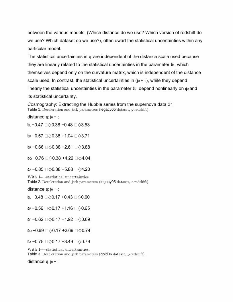
Cosmography: Extracting the Hubble series from the supernova data 31Table 1. Deceleration and jerk parameters (legacy05 dataset, y-redshift).
distance q0 j0 + 0
dL −0.47 �} 0.38 −0.48 �} 3.53
dF −0.57 �} 0.38 +1.04 �} 3.71
dP −0.66 �} 0.38 +2.61 �} 3.88
dQ −0.76 �} 0.38 +4.22 �} 4.04
dA −0.85 �} 0.38 +5.88 �} 4.20With 1-_ statistical uncertainties.Table 2. Deceleration and jerk parameters (legacy05 dataset, z-redshift).
distance q0 j0 + 0
dL −0.48 �} 0.17 +0.43 �} 0.60
dF −0.56 �} 0.17 +1.16 �} 0.65
dP −0.62 �} 0.17 +1.92 �} 0.69
dQ −0.69 �} 0.17 +2.69 �} 0.74
dA −0.75 �} 0.17 +3.49 �} 0.79With 1-_ statistical uncertainties.Table 3. Deceleration and jerk parameters (gold06 dataset, y-redshift).
distance q0 j0 + 0

dL −0.62 �} 0.29 +1.66 �} 2.60
dF −0.78 �} 0.29 +3.95 �} 2.80
dP −0.94 �} 0.29 +6.35 �} 3.00
dQ −1.09 �} 0.29 +8.87 �} 3.20
dA −1.25 �} 0.29 +11.5 �} 3.41With 1-_ statistical uncertainties.Table 4. Deceleration and jerk parameters (gold06 dataset, z-redshift).
distance q0 j0 + 0
dL −0.37 �} 0.11 +0.26 �} 0.20
dF −0.48 �} 0.11 +1.10 �} 0.24
dP −0.58 �} 0.11 +1.98 �} 0.29
dQ −0.68 �} 0.11 +2.92 �} 0.37
dA −0.79 �} 0.11 +3.90 �} 0.39With 1-_ statistical uncertainties.
Cosmography: Extracting the Hubble series from the supernova data 32
10. Model-building uncertainties
The fact that there are such large differences between the cosmological parameters
deduced from the different models should give one pause for concern. These
differences
do not arise from any statistical flaw in the analysis, nor do they in any sense represent
any “systematic” error, rather they are an intrinsic side-effect of what it means to do
a least-squares fit — to a finite-polynomial approximate Taylor series — in a situation
where it is physically unclear as to which if any particular measure of “distance” is
physically preferable, and which particular notion of “distance” should be fed into the
least-squares algorithm. In Appendix A we present a brief discussion of the most salient
mathematical issues.
The key numerical observations are that the different notions of cosmological
distance lead to equally spaced least-squares estimates of the deceleration parameter,
with equal statistical uncertainties; the reason for the equal-spacing of these estimates
being analytically explainable by the analysis presented in Appendix A. Furthermore,
from the results in Appendix A we can explicitly calculate the magnitude of this
modelling ambiguity as
[_q0]modelling = −1 +
"
X
I
zi+j
I
#−1
1j"
X
I
zj
I ln(1 + zI )#
, (81)
while the corresponding formula for y-redshift is
[_q0]modelling = −1 −
"

X
I
yi+j
I
#−1
1j"
X
I
yj
I ln(1 −yI)
#
. (82)
Note that for the quadratic fits we have adopted this requires calculating a (n+1)×(n+1)
matrix, with {i, j} 2 {0, 1, 2}, inverting it, and then taking the inner product between
the first row of this inverse matrix and the relevant column vector. The Einstein
summation convention is implied on the j index. For the z-redshift (if we were to
restrict our z-redshift dataset to z < 1, e.g., using legacy05 or a truncation of gold06) it
makes sense to Taylor series expand the logarithm to alternatively yield
[_q0]modelling = −
X1
k=n+1
(−1)k
k

"
X
I
zi+j
I
#−1
1j"
X
I
zj+k
I#
. (83)
For the y-redshift we do not need this restriction and can simply write
[_q0]modelling =X1
k=n+1
1k"
X
I
yi+j

I
#−1
1j"
X
I
yj+k
I#
. (84)
As an extra consistency check we have independently calculated these quantities
(which
depend only on the redshifts of the supernovae) and compared them with the spacing
we find by comparing the various least-squares analyses. For the n = 2 quadratic fits
these formulae reproduce the spacing reported in tables 1–4. As the order n of the
polynomial increases, it was seen that the differences between deceleration parameter
Cosmography: Extracting the Hubble series from the supernova data 33
estimates based on the different distance measures decreases — unfortunately the size
of the purely statistical uncertainties was simultaneously seen to increase — this being
a side effect of adding terms that are not statistically significant according to the F test.
Thus to minimize “model building ambiguities” one wishes the parameter “ n” to
be as large as possible, while to minimize statistical uncertainties, one does not want to
add statistically meaningless terms to the polynomial.
Note that if one were to have a clearly preferred physically motivated “best”
distance this whole model building ambiguity goes away. In the absence of a clear
physically justifiable preference, the best one can do is to combine the data as per
the discussion in Appendix B, which is based on NIST recommended guidelines [44],

and report an additional model building uncertainty (beyond the traditional purely
statistical uncertainty).
Note that we do limit the modelling uncertainty to that due to considering the five
reasonably standard definitions of distance dA, dQ, dP , dF , and dL. The reasons for
this limitation are partially practical (we have to stop somewhere), and partly
physicsrelated
(these five definitions of distance have reasonably clear physical interpretations,
and there seems to be no good physics reason for constructing yet more notions of
cosmological distance).
Turning to the quantity (j0 + 0), the different notions of distance no longer yield
equally spaced estimates, nor are the statistical uncertainties equal. This is due to the
fact that there is a nonlinear quadratic term involving q0 present in the relation used to
convert the polynomial coefficient b2 into the more physical parameter (j0 + 0). Note
that while for each specific model (choice of distance scale and redshift variable) the
F-test indicates that keeping the quadratic term is statistically significant, the variation
among the models is so great as to make measurements of (j0+0) almost meaningless.
The combined results are reported in tables 5–6. Note that these tables do not yet
include any budget for “systematic” uncertainties.Table 5. Deceleration parameter summary: Statistical plus modelling.
dataset redshift q0 �} _statistical �} _modelling
legacy05 y −0.66 �} 0.38 �} 0.13
legacy05 z −0.62 �} 0.17 �} 0.10
gold06 y −0.94 �} 0.29 �} 0.22
gold06 z −0.58 �} 0.11 } 0.15With 1-_ statistical uncertainties and 1-_ model building uncertainties,no budget for systematic uncertainties.“ ”
Again, we reiterate the fact that there are distressingly large differences between
the cosmological parameters deduced from the different models — this should give one
pause for concern above and beyond the purely formal statistical uncertainties reported
herein.

Cosmography: Extracting the Hubble series from the supernova data 34Table 6. Jerk parameter summary: Statistical plus modelling.
dataset redshift (j0 + 0) } _statistical } _modelling
legacy05 y +2.65 } 3.88 } 2.25
legacy05 z +1.94 } 0.70 } 1.08
gold06 y +6.47 } 3.02 } 3.48
gold06 z +2.03 } 0.31 } 1.29With 1-_ statistical uncertainties and 1-_ model building uncertanties,no budget for systematic uncertainties.“ ”
11. Systematic uncertainties
Beyond the statistical uncertainties and model-building uncertainties we have so far
considered lies the issue of systematic uncertainties. Systematic uncertainties are
extremely difficult to quantify in cosmology, at least when it comes to distance
measurements — see for instance the relevant discussion in [4, 5], or in [6]. What
is less difficult to quantify, but still somewhat tricky, is the extent to which systematics
propagate through the calculation.
11.1. Major philosophies underlying the analysis of statistical uncertainty
When it comes to dealing with systematic uncertainties there are two major philosophies
on how to report and analyze them:
•Treat all systematic uncertainties as though they were purely statistical and report
1-sigma “effective standard uncertainties”. In propagating systematic uncertainties
treat them as though they were purely statistical and uncorrelated with the usual
statistical uncertainties. In particular, this implies that one is to add estimated
systematic and statistical uncertainties in quadrature_2
combined =q
_2
statistical + _2

systematic. (85)
This manner of treating the systematic uncertainties is that currently recommended
by NIST [44], this recommendation itself being based on ISO, CPIM, and
BIPM recommendations. This is also the language most widely used within the
supernova community, and in particular in discussing the gold05 and legacy05
datasets [1, 2, 3, 4, 5], so we shall standardize our language to follow these norms.
•An alternative manner of dealing with systematics (now deprecated) is to carefully
segregate systematic and statistical effects, somehow estimate “credible bounds”
on the systematic uncertainties, and then propagate the systematics through the
calculation — if necessary using interval arithmetic to place “credible bounds” on
the final reported systematic uncertainty. The measurements results would then be
reported as a number with two independent sources of uncertainty — the statistical
Cosmography: Extracting the Hubble series from the supernova data 35
and systematic uncertainties, and within this philosophy there is no justification
for adding statistical and systematic effects in quadrature.
It is important to realise that the systematic uncertainties reported in gold05 and
legacy05 are of the first type: effective equivalent 1-sigma error bars [1, 2, 3, 4, 5].
These
reported uncertainties are based on what in the supernova community are referred to
as “known unknowns”.
(The NIST guidelines [44] also recommend that all uncertainties estimated by
statistical methods should be denoted by the symbol s, not _, and that uncertainties
estimated by non-statistical methods, and combined overall uncertainties, should be
denoted by the symbol u — but this is rarely done in practice, and we shall follow the
traditional abuse of notation and continue to use _ throughout.)
11.2. Deceleration
For instance, assume we can measure distance moduli to within a systematic
uncertainty
_μsystematic over a redshift range _(redshift). If all the measurements are biased high, or
all are biased low, then the systematic uncertainty would affect the Hubble parameter
H0, but would not in any way disturb the deceleration parameter q0. However there may
be a systematic drift in the bias as one scans across the range of observed redshifts.
The
worst that could plausibly happen is that all measurements are systematically biased
high at one end of the range, and biased low at the other end of the range. For data
collected over a finite width _(redshift), this “worst plausible” situation leads to a
systematic uncertainty in the slope of
__
dμdz_
systematic
=
2 _μsystematic
_(redshift)
, (86)
which then propagates to an uncertainty in the deceleration parameter of
_systematic =
2 ln 10
5
__
dμdz_
systematic
=

4 ln 10
5
_μsystematic
_(redshift) _ 1.8
_μsystematic
_(redshift)
. (87)
For the situation we are interested in, if we take at face value the reliability of
the assertion “...we adopt a limit on redshift-dependent systematics to be 5% per
_z = 1” [4], meaning up to 2.5% high at one end of the range and up to 2.5% low
at the other end of the range. A 2.5% variation in distance then corresponds, via
_μD = 5_(ln dL)/ ln 10, to an uncertainty _μsystematic = 0.05 in stellar magnitude. So,
(taking _z = 1), one has to face the somewhat sobering estimate that the “equivalent
1-_ uncertainty” for the deceleration parameter q0 is
_systematic = 0.09. (88)
When working with y-redshift, one really should reanalyze the entire corpus of data
from first principles — failing that, (not enough of the raw data is publicly available),
we shall simply observe that
dz
dy ! 1 as y ! 0, (89)
Cosmography: Extracting the Hubble series from the supernova data 36
and use this as a justification for assuming that the systematic uncertainty in q0 when
using y-redshift is the same as when using z-redshift.
11.3. Jerk
Turning to systematic uncertainties in the jerk, the worst that could plausibly happen
is that all measurements are systematically biased high at both ends of the range, and
biased low at the middle, (or low at both ends and high in the middle), leading to a
systematic uncertainty in the second derivative of
1
2

__
d2μdz2_
systematic_
_(redshift)
2_2
= 2_μsystematic, (90)
where we have taken the second-order term in the Taylor expansion around the
midpoint of the redshift range, and asked that it saturate the estimated systematic
error 2_μsystematic. This implies
__
d2μdz2_
systematic
=
16 _μsystematic
_(redshift)2 , (91)
which then propagates to an uncertainty in the jerk parameter (j0 + 0) of at least_systematic _

3 ln 10
5
__
d2μdz2_
systematic
=
48 ln 10
5
_μsystematic
_(redshift)2 _ 22
_μsystematic
_(redshift)2 . (92)
There are additional contributions to the systematic uncertainty arising from terms
linear and quadratic in q0. They do not seem to be important in the situations we
are interested in so we content ourselves with the single term estimated above. Using
_μsystematic = 0.05 and _z = 1 we see that the “equivalent 1-_ uncertainty” for the
combination (j0 + 0) is:
_systematic = 1.11. (93)
Thus direct cosmographic measurements of the jerk parameter are plagued by very
high systematic uncertainties. Note that the systematic uncertainties calculated in this
section are completely equivalent to those reported in [4].
12. Historical estimates of systematic uncertainty
We now turn to the question of possible additional contributions to the uncertainty,
based on what the NIST recommendations call “type B evaluations of uncertainty” —
namely “any method of evaluation of uncertainty by means other than the statistical
analysis of a series of observations” [44]. (This includes effects that in the supernova

community are referred to as “unknown unknowns”, which are not reported in any of
their estimates of systematic uncertainty.)
The key point here is this: “A type B evaluation of standard uncertainty is usually
based on scientific judgment using all of the relevant information available, which
may include: previous measurement data, etc...” [44]. It is this recommendation that
Cosmography: Extracting the Hubble series from the supernova data 37
underlies what we might wish to call the “historical” estimates of systematic uncertainty
— roughly speaking, we suggest that in the systematic uncertainty budget it is prudent
to keep an extra “historical uncertainty” at least as large as the most recent major
re-calibration of whatever measurement method you are currently using.
Now this “historical uncertainty” contribution to the systematic uncertainty budget
that we are advocating is based on 100 years of unanticipated systematic errors
(“unknown unknowns”) in astrophysical distance scales — from Hubble’s reliance
on mis-calibrated Cephid variables (leading to distance estimates that were about
666% too large), to last decade’s debates on the size of our own galaxy (with up to
15% disagreements being common), to last year’s 5% shift in the high-z supernova
distances [4, 5] — and various other re-calibration events in between. That is, 5%
variations in estimates of cosmological distances on a 2 year time scale seem common,
10% on a 10 year time scale, and 500% or more on an 80 year timescale? A
disinterested outside observer does detect a certain pattern here. (These re-calibrations
are of course not all related to supernova measurements, but they are historical
evidence of how difficult it is to make reliable distance measurements in cosmology.)
Based on the historical evidence we feel that it is currently prudent to budget an
additional “historical uncertainty” of approximately 5% in the distances to the furthest
supernovae, (corresponding to 0.10 stellar magnitudes), while for the nearby
supernovae
we generously budget a “historical uncertainty” of 0%, based on the fact that these
distances have not changed in the last 2 years [4, 5].¶
12.1. Deceleration
This implies

__
dμdz_
historical
=
_μhistorical
_(redshift)
. (94)
Note the absence of a factor 2 compared to equation (86), this is because in this
“historical” discussion we have taken the nearby supernovae to be accurately
calibrated,
whereas in the discussion of systematic uncertainties in equation (86) both nearby and
distant supernovae are subject to “known unknown” systematics. This then propagates
to an uncertainty in the deceleration parameter of
_historical =
2 ln 10
5
__
dμdz_
historical
=
2 ln 10
5

_μhistorical
_(redshift) _ 0.9
_μhistorical
_(redshift)
. (95)¶ Some researchers have argued that the present historical estimates of uncertainty confuse the notion“ ”
of error with that of uncertainty . We disagree. What we are doing here is to use the most recently“ ” “ ”detected (significant) error to estimate one component of the uncertainty this is simply a scientific— “judgment using all of the relevant information available . We should add that other researchers have”argued that our historical uncertainties should be even larger. By using the most recent major recalibrationas our basis for historical uncertainty we feel we are steering a middle course betweenplacing too much versus to little credence in the observational data.
Cosmography: Extracting the Hubble series from the supernova data 38
Noting that a 5% shift in luminosity distance is equivalent to an uncertainty of
_μhistorical = 0.10 in stellar magnitude, this implies an “equivalent 1-_ uncertainty”
for the deceleration parameter q0 is
_historical = 0.09. (96)
This (coincidentally) is equal to the systematic uncertainties based on “known
unknowns”.
12.2. Jerk
Turning to the second derivative a similar analysis implies
1
2
__
d2μdz2_
historical
_(redshift)2 = _μhistorical. (97)

Note the absence of various factors of 2 as compared to equation (90). This is because
we
are now assuming that for “historical” purposes the nearby supernovae are accurately
calibrated and it is only the distant supernovae that are potentially uncertain — thus in
estimating the historical uncertainty the second-order term in the Taylor series is now
to be saturated using the entire redshift range. Thus
__
d2μdz2_
historical
=
2 _μhistorical
_(redshift)2 , (98)
which then propagates to an uncertainty in the jerk parameter of at least_historical _
3 ln 10
5
__
d2μdz2_
historical
=
6 ln 10
5

_μhistorical
_(redshift)2 _ 2.75
_μhistorical
_(redshift)2 . (99)
Again taking _μhistorical = 0.10 this implies an “equivalent 1-_ uncertainty” for the
combination j0 + 0 is
_historical = 0.28. (100)
Note that this is (coincidentally) one quarter the size of the systematic uncertainties
based on “known unknowns”, and is still quite sizable.
The systematic and historical uncertainties are now reported in tables 7–8. The
estimate for systematic uncertainties are equivalent to those presented in [4], which is
largely in accord with related sources [1, 2, 3]. Our estimate for “historical” uncertainties
is likely to be more controversial — with, we suspect, many cosmologists arguing that
our estimates are too generous — and that _historical should perhaps be even larger
than we have estimated. What is not (or should not) be controversial is the need for
some estimate of _historical. Previous history should not be ignored, and as the NIST
guidelines emphasize, previous history is an essential and integral part of making the
scientific judgment as to what the overall uncertainties are.
Cosmography: Extracting the Hubble series from the supernova data 39Table 7. Deceleration parameter summary:Statistical, modelling, systematic, and historical.
dataset redshift q0 } _statistical } _modelling } _systematic } _historical
legacy05 y −0.66 �} 0.38 �} 0.13 �} 0.09 �} 0.09
legacy05 z −0.62 �} 0.17 �} 0.10 �} 0.09 �} 0.09
gold06 y −0.94 �} 0.29 �} 0.22 �} 0.09 �} 0.09
gold06 z −0.58 �} 0.11 �} 0.15 �} 0.09 �} 0.09With 1-_ effective statistical uncertainties for all components.Table 8. Jerk parameter summary:Statistical, modelling, systematic, and historical.
dataset redshift (j0 + 0) } _statistical } _modelling } _systematic } _historical

legacy05 y +2.65 } 3.88 } 2.25 } 1.11 } 0.28
legacy05 z +1.94 } 0.70 } 1.08 } 1.11 } 0.28
gold06 y +6.47 } 3.02 } 3.48 } 1.11 } 0.28
gold06 z +2.03 } 0.31 } 1.29 } 1.11 } 0.28With 1-_ effective statistical uncertainties for all components.
13. Combined uncertainties
We now combine these various uncertainties, purely statistical, modelling, “known
unknown” systematics, and “historical” (“unknown unknowns”). Adopting the NIST
philosophy of dealing with systematics, these uncertainties are to be added in
quadrature [44]. Including all 4 sources of uncertainty we have discussed:
_combined =q
_2
statistical + _2
modelling + _2
systematic + _2
historical. (101)
That the statistical and modelling uncertainties should be added in quadrature is clear
from their definition. Whether or not systematic and historical uncertainties should
be treated this way is very far from clear, and implicitly presupposes that there are
no correlations between the systematics and the statistical uncertainties — within
the “credible bounds” philosophy for estimating systematic uncertainties there is no
justification for such a step. Within the “all errors are effectively statistical” philosophy
adding in quadrature is standard and in fact recommended — this is what is done
in current supernova analyses, and we shall continue to do so here. The combined
uncertainties _combined are reported in tables 9–10.
Cosmography: Extracting the Hubble series from the supernova data 40
14. Expanded uncertainty
An important concept under the NIST guidelines is that of “expanded uncertainty”

Uk = k _combined. (102)
Expanded uncertainty is used when for either scientific or legal/regulatory reasons one
wishes to be “certain” that the actual physical value of the quantity being measured lies
within the stated range. We shall take k = 3, this being equivalent to the well-known
particle physics aphorism “if it’s not three-sigma, it’s not physics”. Note that this is not
an invitation to randomly multiply uncertainties by 3, rather it is a scientific judgment
that if one wishes to be 99.5% certain that something is or is not happening one should
look for a 3-sigma effect. Bitter experience within the particle physics community has
led to the consensus that 3-sigma is the minimum standard one should look for when
claiming “new physics”.+ Thus we take
U3 = 3 _combined. (103)
The best estimates, combined uncertainties _combined, and expanded uncertainties U, are
reported in tables 9–10.Table 9. Deceleration parameter summary:Combined and expanded uncertainties.
dataset redshift q0 �} _combined q0 �} U3
legacy05 y −0.66 �} 0.42 −0.66 �} 1.26
legacy05 z −0.62 �} 0.23 −0.62 �} 0.70
gold06 y −0.94 �} 0.39 −0.94 �} 1.16
gold06 z −0.58 �} 0.23 −0.58 �} 0.68
Table 10. Jerk parameter summary:Combined and expanded uncertainties.
dataset redshift (j0 + 0) �} _combined (j0 + 0) �} U3
legacy05 y +2.65 } 4.63 +2.65 } 13.9
legacy05 z +1.94 } 1.72 +1.94 } 5.17
gold06 y +6.47 } 4.75 +6.47 } 14.2
gold06 z +2.03 } 1.75 +2.03 } 5.26
+ There is now a growing consensus in the particle physics community that 5-sigma should be the newstandard for claiming new physics [45].“ ”
Cosmography: Extracting the Hubble series from the supernova data 41
15. Results
What can we conclude from this? While the “preponderance of evidence” is certainly
that the universe is currently accelerating, q0 < 0, this is not yet a “gold plated”
result. We emphasise the fact that (as is or should be well known) there is an enormous
difference between the two statements:
•“the most likely value for the deceleration parameter is negative”, and
•“there is significant evidence that the deceleration parameter is negative”.
When it comes to assessing whether or not the evidence for an accelerating universe
is physically significant, the first rule of thumb for combined uncertainties is the well
known aphorism “if it’s not three-sigma, it’s not physics”. The second rule is to be
conservative in your systematic uncertainty budget. We cannot in good faith conclude
that the expansion of the universe is accelerating. It is more likely that the expansion
of the universe is accelerating, than that the expansion of the universe is decelerating
— but this is a very long way from having definite evidence in favour of acceleration.
The summary regarding the jerk parameter, or more precisely (j0 + 0), is rather grim
reading, and indicates the need for considerable caution in interpreting the supernova
data. Note that while use of the y-redshift may improve the theoretical convergence
properties of the Taylor series, and will not affect the uncertainties in the distance
modulus or the various distance measures, it does seem to have an unfortunate
sideeffect
of magnifying statistical uncertainties for the cosmological parameters.
As previously mentioned, we have further checked the robustness of our analysis by
first excluding the outlier at z = 1.755, then excluding the so-called “Hubble bubble”
at z < 0.0233 [35, 36], and then excluding both — the precise numerical estimates for
the cosmological parameters certainly change, but the qualitative picture remains as we
have painted it here.
16. Conclusions
Why do our conclusions seem to be so much at variance with currently perceived
wisdom
concerning the acceleration of the universe? The main reasons are twofold:
•Instead of simply picking a single model and fitting the data to it, we have tested
the overall robustness of the scenario by encoding the same physics (H0, q0, j0)
in multiple different ways (dL, dF , dP , dQ, dA; using both z and y) to test the
robustness of the data fitting procedures.
•We have been much more explicit, and conservative, about the role of systematic
uncertainties, and their effects on estimates of the cosmological parameters.
If we only use the statistical uncertainties and the “known unknowns” added in
quadrature, then the case for cosmological acceleration is much improved, and is (in
some cases we study) “statistically significant at three-sigma”, but this does not mean
that such a conclusion is either robust or reliable. (By “cherry picking” the data, and
Cosmography: Extracting the Hubble series from the supernova data 42
the particular way one analyzes the data, one can find statistical support for almost any
conclusion one wants.)
The modelling uncertainties we have encountered depend on the distance variable
one chooses to do the least squares fit (dL, dF , dP , dQ, dA). There is no good physics
reason for preferring any one of these distance variables over the others. One can
always minimize the modelling uncertainties by going to a higher-order polynomial —
unfortunately at the price of unacceptably increasing the statistical uncertainties —
and we have checked that this makes the overall situation worse. This does however
suggest that things might improve if the data had smaller scatter and smaller statistical
uncertainties: We could then hope that the F-test would allow us to go to a cubic
polynomial, in which case the dependence on which notion of distance we use for
leastsquares
fitting should decrease.
We wish to emphasize the point that, regardless of one’s views on how to
combine formal estimates of uncertainty, the very fact that different distance
scales yield data-fits with such widely discrepant values strongly suggests the
need for extreme caution in interpreting the supernova data.
Though we have chosen to work on a cosmographic framework, and so minimize the
number of physics assumptions that go into the model, we expect that similar modelling
uncertainties will also plague other more traditional approaches. (For instance, in the
present-day consensus scenario there is considerable debate as to just when the
universe
switches from deceleration to acceleration, with different models making different
statistical predictions [46].) One lesson to take from the current analysis is that purely
statistical estimates of error, while they can be used to make statistical deductions
within the context of a specific model, are often a bad guide as to the extent to which
two different models for the same physics will yield differing estimates for the same
physical quantity.
There are a number of other more sophisticated statistical methods that might
be applied to the data to possibly improve the statistical situation. For instance,
ridge regression, robust regression, and the use of orthogonal polynomials and loess
curves. However one should always keep in mind the difference between accuracy and
precision [37]. More sophisticated statistical analyses may permit one to improve
the precision of the analysis, but unless one can further constrain the systematic
uncertainties such precise results will be no more accurate than the current situation.
Excessive refinement in the statistical analysis, in the absence of improved bounds on
the systematic uncertainties, is counterproductive and grossly misleading.
However, we are certainly not claiming that all is grim on the cosmological front —
and do not wish our views to be misinterpreted in this regard—there are clearly parts of
cosmology where there is plenty of high-quality data, and more coming in, constraining
and helping refine our models. But regarding some specific cosmological questions the
catch cry should still be “Precision cosmology? Not just yet” [47].
Cosmography: Extracting the Hubble series from the supernova data 43
In particular, in order for the current technique to become a tool for precision
cosmology, we would need more data, smaller scatter in the data, and smaller
uncertainties. For instance, by performing the F-test we found that it was almost
always statistically meaningless to go beyond quadratic fits to the data. If one can
obtain an improved dataset of sufficient quality for cubic fits to be meaningful, then
ambiguities in the deceleration parameter are greatly suppressed.

In closing, we strongly encourage readers to carefully contemplate figures 7–10 as
an inoculation against over-interpretation of the supernova data. In those figures we
have split off the linear part of the Hubble law (which is encoded in the intercept)
and chosen distance variables so that the slope (at redshift zero) of whatever curve one
fits to those plots is directly proportional to the acceleration of the universe (in fact
the slope is equal to −q0/2). Remember that these plots only exhibit the statistical
uncertainties. Remembering that we prefer to work with natural logarithms, not stellar
magnitudes, one should add systematic uncertainties of �}[ln(10)/5] ×(0.05) _ 0.023
to these statistical error bars, presumably in quadrature. Furthermore a good case can
be made for adding an additional “historical” uncertainty, using the past history of the
field to estimate the “unknown unknowns”.
Ultimately however, it is the fact that figures 7–10 do not exhibit any
overwhelmingly obvious trend that makes it so difficult to make a robust and
reliable estimate of the sign of the deceleration parameter.
Appendix A. Some ambiguities in least-squares fitting
Let us suppose we have a function f(x), and want to estimate f(x) and its derivatives
at zero via least squares. For any g(x) we have a mathematical identity
f(x) = [f(x) −g(x)] + g(x), (A.1)
and for the derivatives
f(m)(0) = [f −g](m)(0) + g(m)(0). (A.2)
Adding and subtracting the same function g(x) makes no difference to the underlying
function f(x), but it may modify the least squares estimate for that function. That
is: Adding and subtracting a known function to the data does not commute with the
process of performing a finite-polynomial least-squares fit. Indeed, let us approximate
[f(x) −g(x)] =
Xn
i=0
bf−g,i xi + _. (A.3)
Then given a set of observations at points (fI , xI) we have (in the usual manner) the
equations (for simplicity of the presentation all statistical uncertainties _ are set equal
for now)
[fI −g(xI)] =
Xn
i=0
ˆbf−g,i xi
I + _I , (A.4)
Cosmography: Extracting the Hubble series from the supernova data 44
where we want to minimizeX
I
|_I |2. (A.5)
This leads toX
I
[fI −g(xI)]xj
I =Xn
i=0
ˆbf−g,iX
I
xi+j
I , (A.6)
whence
ˆb
f−g,i ="
X
I
xi+j
I
#−1 X
I
[fI −g(xI)]xj
I , (A.7)
where the square brackets now indicate an (n + 1) ×(n + 1) matrix, and there is an
implicit sum on the j index as per the Einstein summation convention. But we can
re-write this as
ˆb
f−g,i =ˆbf,i −
"
X
I
xi+j
I
#−1 X
I
[g(xI)]xj
I , (A.8)
relating the least-squares estimates of bf,i and bf−g,i. Note that by construction i _ n.
If we now use this to estimate f(i)(0), we see:
ˆ f(i)
[f−g]+g(0) = ˆ f(i)
f−g(0) + g(i)(0), (A.9)
whence
ˆ f(i)
[f−g]+g(0) = ˆ f(i)(0) −i!
"
X
I
xi+j
I
#−1 X
I
[g(xI)]xj
I + g(i)(0), (A.10)
where ˆ f(i)(0) is the “naive” estimate of f(i)(0) obtained by simply fitting a polynomial
to f itself, and ˆ f(i)
[f−g]+g(0) is the “improved” estimate obtained by first subtracting g(x),
fitting f(x)−g(x) to a polynomial, and then adding g(x) back again. Note the formula
for the shift of the estimate of the ith derivative of f(x) is linear in the function g(x)
and its derivatives. In general this is the most precise statement we can make — the
process of finding a truncated Taylor series simply does not commute with the process
of performing a least squares fit.
We can gain some additional insight if we use Taylor’s theorem to write
g(x) =X1
k=0
g(k)(0)
k!
xk =Xn
k=0
g(k)(0)
k!
xk +X1
k=n+1
g(k)(0)
k!
xk, (A.11)
where we temporarily suspend concerns regarding convergence of the Taylor series.
Then
ˆ f(i)
[f−g]+g(0) = ˆ f(i)(0) + g(i)(0) (A.12)
−i!
"
X
I
xi+j

I
#−1 X
I(
Xn
k=0
g(k)(0)
j!xk
I +X1
k=n+1
g(k)(0)
j!xk
I)
xj
I .
Cosmography: Extracting the Hubble series from the supernova data 45
So
ˆ f(i)
[f−g]+g(0) = ˆ f(i)(0) + g(i)(0) (A.13)
−i!
"
X
I
xi+j
I
#−1 (
Xn
k=0
g(k)(0)
k!X
I
xj+k
I +X1
k=n+1
g(k)(0)
k!X
I
xj+k
I)
,
whence
ˆ f(i)
[f−g]+g(0) = ˆ f(i)(0) + g(i)(0) −i!
Xn
k=0
g(k)(0)
k!"
X
I
xi+j
I
#−1 "
X
I
xj+k
I#
−i!
X1
k=n+1
g(k)(0)
k!"

X
I
xi+j
I
#−1X
I
xj+k
I . (A.14)
But two of these matrices are simply inverses of each other, so in terms of the
Kronecker
delta
ˆ f(i)
[f−g]+g(0) = ˆ f(i)(0) + g(i)(0) −i!
Xn
k=0
g(k)(0)
k!_ik
−i!
X1
k=n+1
g(k)(0)
k!"
X
I

xi+j
I
#−1X
I
xj+k
I , (A.15)
which now leads to significant cancellations
ˆ f(i)
[f−g]+g(0) = ˆ f(i)(0) −i!
X1
k=n+1
g(k)(0)
k!"
X
I
xi+j
I
#−1X
I
xj+k
I . (A.16)
This is the best (ignoring convergence issues) that one can do in the general case.
Note the formula for the shift of the estimate of the ith derivative of f(x) is linear in
the derivatives of the function g(x), and that it starts with the (n + 1)th derivative.
Consequently as the order n of the polynomial used to fit the data increases there are
fewer terms included in the sum, so the difference between various estimates of the

derivatives becomes smaller as more terms are added to the least squares fit.
In the particular situation we discuss in the body of the article
f(x) ! ˜ μ = ln
_
d(z)
z Mpc_
; g(x) !K
2
ln(1 + z); K 2 Z; (A.17)
or a similar formula in terms of the y-redshift. Consequently, from equation (A.10),
particularized to our case
ˆ˜μ(i)
K (0) = ˆ˜μ(i)
(0) +K
2
[ln(1 + z)](i)(0) −
K i!
2"
X
I

zi+j
I
#−1 "
X
I
zj
I ln(1 + zI )#
. (A.18)
Then the “gap” between any two adjacent estimates for ˆ˜μ(i)
K (0) corresponds to taking
_K = 1 and so
_ˆ˜μ(i)
(0) =
(−1)i−1 (i −1)!
2 −
i!
2"
X
I
zi+j
I
#−1 "

X
I
zj
I ln(1 + zI )#
. (A.19)
Cosmography: Extracting the Hubble series from the supernova data 46
But then for the particular case i = 1 which is of most interest to us
ˆ˜μ(1)
K (0) = ˆ˜μ(1)
(0) +K
2 −
K
2"
X
I
zi+j
I
#−1
1j"

X
I
zj
I ln(1 + zI)#
, (A.20)
and
_ˆ˜μ(1)
(0) =
1
2 −
1
2"
X
I
zi+j
I
#−1
ij"
X
I
zj

I ln(1 + zI)#
. (A.21)
By Taylor series expanding the logarithm, and reindexing the terms, this can also be
recast as
ˆ˜μ(i)
K (0) = ˆ˜μ(i)
(0) +
K i!
2X1
k=n+1
(−1)k
k"
X
I
zi+j
I
#−1X
I
zj+k
I , (A.22)
whence
ˆ˜μ(1)

K (0) = ˆ˜μ(1)
(0) +K
2X1
k=n+1
(−1)k
k"
X
I
zi+j
I
#−1
1jX
I
zj+k
I , (A.23)
and
_ˆ˜μ(1)
(0) =
1
2X1

k=n+1
(−1)k
k"
X
I
zi+j
I
#−1
1jX
I
zj+k
I , (A.24)
(Because of convergence issues, if we work with z-redshift these last three formulae
make sense only for supernovae datasets where we restrict ourselves to zI < 1, working
in y-redshift no such constraint need be imposed.) Now relating this to the modelling
ambiguity in q0, we have
[_q0]modelling = −2 _ˆ˜μ
(1)
(0), (A.25)
so that
[_q0]modelling = −1 +
"
X
I

zi+j
I
#−1
1j"
X
I
zj
I ln(1 + zI )#
. (A.26)
By Taylor-series expanding the logarithm, modulo convergence issues discussed
above,
this can also be expressed as:
[_q0]modelling = −
X1
k=n+1
(−1)k
k"
X
I
zi+j
I

#−1
1j"
X
I
zj+k
I#
. (A.27)
In particular, without further calculation, these results collectively tell us that the
different estimates for q0 will always be evenly spaced, and it suggests that as n ! 1
the differences will become smaller. This is actually what is seen in the data analysis
we performed. If we were to have a good physics reason for choosing one particular
definition of distance as being primary, we would use that for the least squares fit, and
the other ways of estimating the derivatives would be “biased” — but in the current
situation we have no physically preferred “best” choice of distance variable.
Cosmography: Extracting the Hubble series from the supernova data 47
Appendix B. Combining measurements from different models
Suppose one has a collection of measurements Xa, each of which is represented by a
random variable ˆXa with mean μa = E( ˆXa) and variance _2
a = E([ ˆXa −μa]2). How
should one then combine these measurements into an overall “best estimate”?
If we have no good physics reason to reject one of the measurements then the best
we can do is to describe the combined measurement process by a random variable ˆXAˆ
where Aˆ is now a discrete random variable that picks one of the measurement
techniques

with some probability pa. More precisely
Prob(Aˆ = a) = pa, (B.1)
where the values pa are for now left arbitrary. Then
μ = E( ˆXAˆ) =X
a
pa E( ˆXa) =X
a
pa μa, (B.2)
and
E( ˆX 2
Aˆ) =X
a
pa E( ˆXa)2 =X
a
pa (_2
a + μ2
a). (B.3)
But equally well
E( ˆX 2
Aˆ) = _2 + μ___________2, (B.4)
so that overall
μ =

X
a
pa μa, (B.5)
and
_2 =X
a
pa _2
a +X
a
pa (μa −μ)2. (B.6)
This lets us split the overall variance into the contribution from the purely statistical
uncertanties on the individual measurements
_statistical =sX
a
pa _2
a, (B.7)
plus the “modelling ambiguity” arising from different ways of modelling the same physics
_modelling =sX
a
pa (μa −μ)2. (B.8)
In the particular case we are interested in we have 5 different ways of modelling
distance

and no particular reason for choosing one definition of measurement over all the others
so it is best to take pa = 1/5.
Furthermore in the case of the estimates for the deceleration parameter, all
individual estimates have the same statistical uncertainty, and the estimates are equally
spaced with a gap _:
_a = _0; μa = μP + n_; n 2 {−2,−1, 0, 1, 2}. (B.9)
Cosmography: Extracting the Hubble series from the supernova data 48
Therefore
μ = μP ; _statistical = _0; _modelling = p2 _. (B.10)
For estimates of the jerk, we no longer have the simple equal-spacing rule and equal
statistical uncertainties rule, but there is still no good reason for preferring one distance
surrogate over all the others so we still take pa = 1/5 and the estimate obtained from
the combined measurements satisfies
μ =P
a μa
5
; _statistical =rP
a _2
a
5
; _modelling =rP
a(μa −μ)2
5
. (B.11)

These formulae are used to calculate the statistical and modelling uncertainties reported
in tables 5–6 and 7–8 . Note that by definition the combined purely statistical and
modelling uncertainties are to be added in quadrature
_ =q
_2
statistical + _2
modelling. (B.12)
This discussion does not yet deal with the estimated systematic uncertainties
(“known unknowns”) or “historically estimated” systematic uncertainties (“unknown
unknowns”).
Acknowledgments
This Research was supported by the Marsden Fund administered by the Royal Society
of New Zealand. CC was also supported by a Victoria University of Wellington
Postgraduate scholarship.
References[1] P. Astier et al., The Supernova Legacy Survey: Measurement of “ M, _ and w from the FirstYear Data Set , Astron. Astrophys. ” 447 (2006) 31 [arXiv:astro-ph/0510447].Electronic data available at http://snls.in2p3.fr/conf/papers/cosmo1/[2] SNLS Super Nova Legacy Survey, — http://legacy.astro.utoronto.ca/ http://cfht.hawaii.edu/SNLS/Electronic data available at http://snls.in2p3.fr/conf/papers/cosmo1/[3] A. G. Riess et al., Type Ia Supernova Discoveries at “ z > 1 From the Hubble Space Telescope:Evidence for Past Deceleration and Constraints on Dark Energy Evolution , arXiv:astroph/”0402512.Electronic data available at http://braeburn.pha.jhu.edu/˜ariess/R06/[4] A. G. Riess et al., New Hubble Space Telescope Discoveries of Type Ia Supernovae at “ z > 1:Narrowing Constraints on the Early Behavior of Dark Energy , arXiv:astro-ph/0611572.”Electronic data available at http://braeburn.pha.jhu.edu//˜ariess/R06/[5] S. Jha, A. G. Riess and R. P. Kirshner, Improved Distances to Type Ia Supernovae with Multicolor“Light Curve Shapes: MLCS2k2 , arXiv:astro-ph/0612666.”Electronic data available at http://astro.berkeley.edu//˜saurabh/mlcs2k2/[6] W. M. Wood-Vasey et al., Observational Constraints on the Nature of the Dark Energy: First“Cosmological Results from the ESSENCE Supernova Survey, arXiv:astro-ph/0701041.”
[7] S. Weinberg, Gravitation and cosmology: Principles and applications of the general theory of
relativity, (Wiley, New York, 1972).
[8] P. J. E. Peebles, Principles of physical cosmology, Princeton University Press, 1993.
Cosmography: Extracting the Hubble series from the supernova data 49[9] T. Chiba and T. Nakamura, The luminosity distance, the equation of state, and the geometry of“the universe , Prog. Theor. Phys. ” 100 (1998) 1077 [arXiv:astro-ph/9808022].
[10] V. Sahni, T. D. Saini, A. A. Starobinsky and U. Alam, Statefinder a new geometrical diagnostic“ –of dark energy , JETP Lett. ” 77 (2003) 201 [Pisma Zh. Eksp. Teor. Fiz. 77 (2003) 249][arXiv:astro-ph/0201498].[11] M. Visser, Jerk, snap, and the cosmological equation of state , Class. Quant. Grav. “ ” 21 (2004)2603 [arXiv:gr-qc/0309109].[12] M. Visser, Cosmography: Cosmology without the Einstein equations , Gen. Rel. Grav. “ ” 37 (2005)1541 [arXiv:gr-qc/0411131].[13] D. Rapetti, S. W. Allen, M. A. Amin and R. D. Blandford, A kinematical approach to dark“energy studies , arXiv:astro-ph/0605683.”[14] R. D. Blandford, M. Amin, E. A. Baltz, K. Mandel and P. J. Marshall, Cosmokinetics ,“ ”arXiv:astro-ph/0408279.[15] C. Shapiro and M. S. Turner, What Do We Really Know About Cosmic Acceleration? ,“ ”arXiv:astro-ph/0512586.[16] R. R. Caldwell and M. Kamionkowski, Expansion, Geometry, and Gravity , arXiv:astroph/“ ”0403003.[17] O. Elgaroy and T. Multamaki, Bayesian analysis of Friedmannless cosmologies , JCAP “ ” 0609(2006) 002 [arXiv:astro-ph/0603053].[18] H. K. Jassal, J. S. Bagla and T. Padmanabhan, Observational constraints on low redshift evolution“of dark energy: How consistent are different observations? , Phys. Rev. D ” 72 (2005) 103503[arXiv:astro-ph/0506748].[19] H. K. Jassal, J. S. Bagla and T. Padmanabhan, The vanishing phantom menace , arXiv:astroph/“ ”0601389.[20] T. R. Choudhury and T. Padmanabhan, Cosmological parameters from supernova observations:A Critical comparison of three data sets. Astron. Astrophys. 429 (2005) 807 [arXiv:astroph/0311622].[21] T. Padmanabhan and T. R. Choudhury, A theoretician s analysis of the supernova data and the“ ’limitations in determining the nature of dark energy , Mon. Not. Roy. Astron. Soc. ” 344 (2003)823 [arXiv:astro-ph/0212573].[22] V. Barger, Y. Gao and D. Marfatia, Accelerating cosmologies tested by distance measures , Phys.“ ”Lett. B 648 (2007) 127 [arXiv:astro-ph/0611775].[23] E. P. Hubble, A relation between distance and radial velocity among extra-galactic nebulae ,“ ”Proc. Natl. Acad. Sci. USA 15 (1929)168173.[24] R. P. Kirshner, Hubble s diagram and cosmic expansion , Proc. Natl. Acad. Sci. USA “ ’ ” 101 (2004)8 13.–[25] W.-M. Yao et al., Review of Particle Properties , Journal of Physics G 33, 1 (2006).“ ”Online version at http://pdg.lbl.gov/[26] D. W. Hogg, Distance measures in cosmology, arXiv:astro-ph/9905116.“ ”
[27] R. D Inverno, ’ Introducing Einstein’s relativity, (Oxford University Press, 1992).[28] G. F. R. Ellis and T. Rothman, Lost horizons , American Journal of Physics “ ” 61 (1993) 883 893.–[29] M. Chevallier and D. Polarski, Accelerating universes with scaling dark matter , Int. J. Mod.“ ”Phys. D 10 (2001) 213 [arXiv:gr-qc/0009008].[30] E. V. Linder, Probing gravitation, dark energy, and acceleration , Phys. Rev. D “ ” 70 (2004) 023511[arXiv:astro-ph/0402503].[31] E. V. Linder, Biased Cosmology: Pivots, Parameters, and Figures of Merit , arXiv:astroph/“ ”0604280.[32] B. A. Bassett, P. S. Corasaniti and M. Kunz, The essence of quintessence and the cost of“compression , Astrophys. J. ” 617, L1 (2004) [arXiv:astro-ph/0407364].[33] D. Martin and A. Albrecht, Talk about pivots , arXiv:astro-ph/0604401.“ ”[34] S. Nesseris and L. Perivolaropoulos, Tension and Systematics in the Gold06 SnIa Dataset ,“ ”
Cosmography: Extracting the Hubble series from the supernova data 50arXiv:astro-ph/0612653.[35] I. Zehavi, A. G. Riess, R. P. Kirshner and A. Dekel, A Local Hubble Bubble from SNe Ia? ,“ ”Astrophys. J. 503 (1998) 483 [arXiv:astro-ph/9802252].[36] R. Giovanelli, D. Dale, M. Haynes, E. Hardy and L. Campusano, No Hubble Bubble in the Local“Universe , arXiv:astro-ph/9906362.”[37] P. R. Bevington, Data reduction and analysis in the physical sciences, (McGraw Hill, New York,–1969).
[38] N. R. Draper and H. Smith, Applied regression analysis, (Wiley, New York, 1998).

[39] D. C. Montgomery, E. A. Peck, and G. G. Vining, Introduction to linear regression analysis,(Wiley, New York, 2001).
[40] R. D. Cook and S. Weisberg, Applied regression including computing and graphics, (Wiley, NewYork, 1999).
[41] W. J. Kennedy, Jr. and J. E. Gentle, Statistical computing, (Marcel Dekker, New York, 1980).
[42] R. J. Carroll and D. Rupert, Transformation and weighting in regression, (Chapman and Hall,London, 1998),
[43] G. J. S. Ross, Nonlinear estimation, (Spinger Verlag, New York, 1990).–[44] Guidelines for Evaluating and Expressing the Uncertainty of NIST Measurement Results , Barry“ ”N. Taylor and Chris E. Kuyatt, NIST Technical Note 1297.Online version available as http://physics.nist.gov/cuu/Uncertainty/index.html[45] A. Signal, private communication.[46] J. J¨onsson, A. Goobar, R. Amanullah and L. Bergstr¨om, No evidence for Dark Energy“Metamorphosis? , JCAP ” 0409 (2004) 007 [arXiv:astro-ph/0404468].[47] S. L. Bridle, O. Lahav, J. P. Ostriker and P. J. Steinhardt, Precision Cosmology? Not Just Yet ,“ ”Science 299 (2003) 1532 [arXiv:astro-ph/0303180].