Cosmology I

Hannu Kurki-Suonio

Fall 2020

Preface

These are the lecture notes for my Cosmology course at the University of Helsinki. I first lecturedCosmology at the Helsinki University of Technology in 1996 and then at University of Helsinkifrom 1997 to 2009. Syksy Rasanen taught the course from 2010 to 2015. I have lectured thecourse again since 2016. These notes are based on my notes from 2009, but I have adopted someimprovements made by Syksy.

A difficulty in teaching cosmology is that some very central aspects of modern cosmology relyon rather advanced physics, like quantum field theory in curved spacetime. On the other hand,the main applications of these aspects can be discussed in relatively simple terms, so requiringstudents to have such background would seem overkill, and would prevent many interestedstudents in getting a taste of this exciting and important subject. Thus I am assuming just thestandard bachelor level theoretical physics background (mechanics, special relativity, quantummechanics, statistical physics). The more advanced theories that cosmology relies on, generalrelativity and quantum field theory, are reviewed as a part of this course to a sufficient extent,that we can go on. This represents a compromise which requires from the student an acceptanceof some results without a proper derivation. Even a quantum mechanics or statistical physicsbackground is not necessary, if the student is willing to accept some results taken from these fields(in the beginning of Chapter 4). As mathematical background, Cosmology I requires integraland differential calculus (as taught in Matemaattiset apuneuvot I, II). Cosmology II requiresalso Fourier analysis and spherical harmonic analysis (Fysiikan matemaattiset menetelmat I,II).

The course is divided into two parts. In Cosmology I, the universe is discussed in termsof the homogeneous and isotropic approximation (the Friedmann–Robertson–Walker model),which is good at the largest scales and in the early universe. In Cosmology II, deviations fromthis homogeneity and isotropy, i.e., the structure of the universe, are discussed. I thank ElinaKeihanen, Jussi Valiviita, Ville Heikkila, Reijo Keskitalo, and Elina Palmgren for preparingsome of the figures and doing the calculations behind them.

I try to update these notes each time the course is lectured. This version of Cosmology Iwas updated in August 2019, for the coming fall 2019 course.

– Hannu Kurki-Suonio, August 2019

1 Introduction

Cosmology is the study of the universe as a whole, its structure, its origin, and its evolution.Cosmology is based on observations, mostly astronomical, and laws of physics. These lead

naturally to the standard framework of modern cosmology, the Hot Big Bang.As a science, cosmology has a severe restriction: there is only one universe.1 We cannot

make experiments in cosmology, and observations are restricted to a single object: the Universe.Thus we can make no comparative or statistical studies among many universes. Moreover, weare restricted to observations made from a single location, our solar system. It is quite possiblethat due to this special nature of cosmology, some important questions can never be answered.

Nevertheless, the last few decades have seen a remarkable progress in cosmology, as a sig-nificant body of relevant observational data has become available with modern astronomicalinstruments. We now have a good understanding of the overall history2 and structure of theuniverse, but important open questions remain, e.g., the nature of dark matter and dark energy.Hopefully observations with more advanced instruments will resolve many of these questions inthe coming decades.

The fundamental observation behind the big bang theory was the redshift of distant galaxies.Their spectra are shifted towards longer wavelengths. The further out they are, the larger isthe shift. This implies that they are receding away from us; the distance between them andus is increasing. According to general relativity, we understand this as the expansion of theintergalactic space itself, not as actual motion of the galaxies. As the space expands, thewavelength of light traveling through space expands also.3

This expansion appears to be uniform over large scales: the whole universe expands at thesame rate.4 We describe this expansion by a time-dependent scale factor, a(t). Starting from theobserved present value of the expansion rate, H ≡(da/dt)/a≡ a/a, and knowledge of the energycontent of the universe, we can use general relativity to calculate a(t) as a function of time. Theresult is, using the standard model of particle physics for the energy content at high energies,that a(t) → 0 about 14 billion years ago (I use the American convention, adopted now also bythe British, where billion ≡ 109). At this singularity, the “beginning” of the big bang, which wechoose as the origin of our time coordinate, t = 0, the density of the universe ρ → ∞. In reality,we do not expect the standard model of particle physics to be applicable at extremely highenergy densities. Thus there should be modifications to this picture at the very earliest times,probably just within the first nanosecond. A popular modification, discussed in CosmologyII, is cosmological inflation, which extends these earliest times, possibly, like in the ”eternalinflation” model, infinitely (although usually inflation is thought to last only a small fraction ofa second). At the least, when the density becomes comparable to the so called Planck density,ρPl ∼ 1096 kg/m3, quantum gravitational effects should be large, so that general relativity itself

1There may, in principle, exist other universes, but they are not accessible to our observation. We spell Universewith a capital letter when we refer specifically to the universe we live in, wheres we spell it without a capitalletter, when we refer to the more general or theoretical concept of the universe. In Finnish, ‘maailmankaikkeus’is not capitalized.

2Except for the very beginning.3These are not the most fundamental viewpoints. In general relativity the universe is understood as a four-

dimensional curved spacetime, and its separation into space and time is a coordinate choice, based on convenience.The concepts of expansion of space and photon wavelength are based on such a coordinate choice. The mostfundamental aspect is the curvature of spacetime. At large scales, the spacetime is curved in such a way thatit is convenient to view this curvature as expansion of space, and in the related coordinate system the photonwavelength is expanding at the corresponding rate.

4This applies only at distance scales larger than the scale of galaxy clusters, about 10 Mpc. Bound systems,e.g., atoms, chairs, you and me, the Earth, the solar system, galaxies, or clusters of galaxies, do not expand.The expansion is related to the overall averaged gravitational effect of all matter in the universe. Within boundsystems local gravitational effects are much stronger, so this overall effect is not relevant.

1

1 INTRODUCTION 2

is no longer valid. To describe this Planck era, we would need a theory of quantum gravity,which we do not have.5 Thus these earliest times, including t = 0, have to be excluded fromthe scientific big bang theory. Nevertheless, when discussing the universe after the Planck eraand/or after inflation we customarily set the origin of the time coordinate t = 0, where thestandard model solution would have the singularity.

Thus the proper way to understand the term “big bang”, is not as some event by which theuniverse started or came into existence, but as a period in the early universe, when the universewas very hot,6 very dense, and expanding rapidly.7 Moreover, the universe was then filled withan almost homogeneous “primordial soup” of particles, which was in thermal equilibrium for along time. Therefore we can describe the state of the early universe with a small number ofthermodynamic variables, which makes the time evolution of the universe calculable.

1.1 Misconceptions

There are some popular misconceptions about the big bang, which we correct here:The universe did not start from a point. The part of the universe which we can observe

today was indeed very small at very early times, possibly smaller than 1 mm in diameter at theearliest times that can be sensibly discussed within the big bang framework. And if the inflationscenario is correct, even very much smaller than that before (or during earlier parts of) inflation,so in that sense the word “point” may be appropriate. But the universe extends beyond whatcan be observed today (beyond our “horizon”), and if the universe is infinite (we do not knowwhether the universe is finite or infinite), in current models it has always been infinite, from thevery beginning.

As the universe expands it is not expanding into some space “around” the universe. Theuniverse contains all space, and this space itself is “growing larger”.8

1.2 Units and terminology

We shall use natural units where c = ~ = kB = 1.

1.2.1 c = 1

Relativity theory unifies space and time into a single concept, the 4-dimensional spacetime. Itis thus natural to use the same units for measuring distance and time. Since the (vacuum)speed of light is c = 299 792 458m/s, we set 1 s ≡ 299 792 458m, so that 1 second = 1 lightsecond, 1 year = 1 light year, and c = 1.9 Velocity is thus a dimensionless quantity, and smallerthan one10 for massive objects. Energy and mass have now the same dimension, and Einstein’s

5String theory is a candidate for the theory of quantum gravity. It is, however, very difficult to calculatedefinite predictions for the very early universe from string theory. This is a very active research area at present,but remains quite speculative.

6The realization that the early universe must have had a high temperature did not come immediately after thediscovery of the expansion. The results of big bang nucleosynthesis and the discovery of the cosmic microwavebackground are convincing evidence that the Big Bang was Hot.

7There is no universal agreement among cosmologists about what time period the term ”big bang” refers to.My convention is that it refers to the time from the end of inflation (or from whenever the standard hot big bangpicture becomes valid) until recombination, so that it is actually a 370-000-year-long period, still short comparedto the age of the universe.

8If the universe is infinite, we can of course not apply this statement to the volume of the entire universe,which is infinite, but it applies to finite parts of the universe.

9Most cosmological quantities are not known to better than 3-digit accuracy. In these notes I give more digitsfor many quantities, especially when they are known, so that round-off errors do not accumulate if these quantitiesare used in calculations.

10In the case of “physical” (as opposed to “coordinate”) velocities.

1 INTRODUCTION 3

famous equivalence relation between mass and energy, E = mc2, becomes E = m. This justifiesa change in terminology; since mass and energy are the same thing, we do not waste two wordson it. As is customary in particle physics we shall use the word “energy”, E, for the abovequantity. By the word “mass”, m, we mean the rest mass. Thus we do not write E = m, butE = mγ, where γ = 1/

√1− v2. The difference between energy and mass, E −m, is the kinetic

energy of the object.11

1.2.2 kB = 1

Temperature, T , is a parameter describing a thermal equilibrium distribution. The formula forthe equilibrium occupation number of energy level E includes the exponential form eβE , wherethe parameter β = 1/kBT . The only function of the Boltzmann constant, kB = 1.380 649 ×10−23 J/K, is to convert temperature into energy units. Since we now decide to give temperaturesdirectly in energy units, kB becomes unnecessary. We define 1K = 1.380 649 × 10−23 J, or

1 eV = 11 604.5K = 1.782 662 × 10−36 kg = 1.602 177 × 10−19 J. (1)

Thus kB = 1, and the exponential form is just eE/T .

1.2.3 ~ = 1

The third simplification in the natural system of units is to set the Planck constant ~ ≡ h/2π = 1.This makes the dimension of mass and energy 1/time or 1/distance. This time and distancegive the typical time and distance scales quantum mechanics associates with the particle energy.For example, the energy of a photon E = ~ω = ω = 2πν is equal to its angular frequency. Sinceh = 6.626 070 15 × 10−34 Js in SI units, we have

1 kg = 2.842 788 × 1042 m−1 = 8.522 465 × 1050 s−1

1 eV = 5067 730.7m−1 = 1.519 267 × 1015 s−1 . (2)

A useful relation to remember is~ = 1 ≈ 197MeV fm (3)

(more precisely, the number is 197.327), where we have the energy scale ∼ 200MeV and lengthscale ∼ 1 fm of strong interactions.

Equations become now simpler and the physical relations more transparent, since we do nothave to include the above fundamental constants. This is not a completely free lunch, however;we often have to do conversions among the different units to give our answers in familiar units.

1.2.4 Astronomical units

A common unit of mass and energy is the solar mass, M⊙ = 1.988 48 ± 9× 1030 kg [1],12 and acommon unit of length is parsec, 1 pc = 3.261 564 light years = 3.085 678×1016 m. One parsecis defined as the distance from which 1 astronomical unit (AU, the distance between the Earthand the Sun) forms an angle of one arcsecond, 1′′. More common in cosmology is 1Mpc =106 pc, which is a typical distance between neighboring galaxies. For angles, 1 degree (1) = 60arcminutes (60′) = 3600 arcseconds (3600′′).

1 INTRODUCTION 4

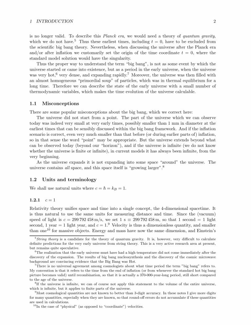
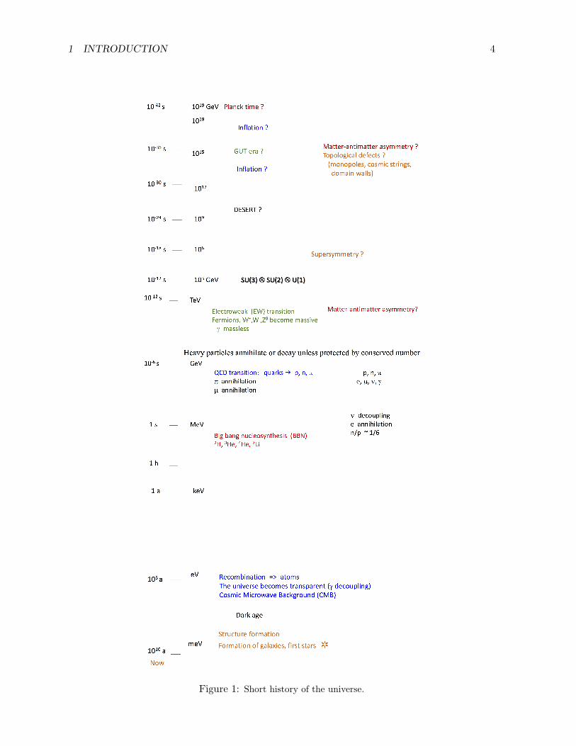
Figure 1: Short history of the universe.

1 INTRODUCTION 5

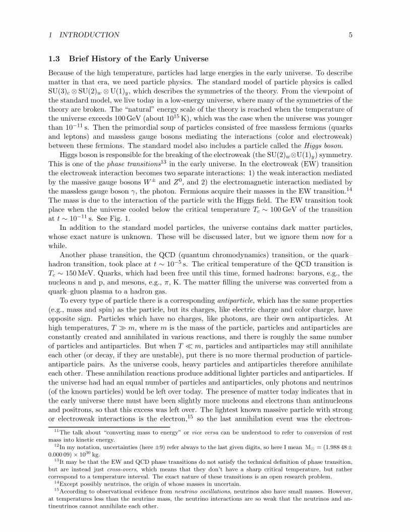
1.3 Brief History of the Early Universe

Because of the high temperature, particles had large energies in the early universe. To describematter in that era, we need particle physics. The standard model of particle physics is calledSU(3)c ⊗ SU(2)w ⊗U(1)y , which describes the symmetries of the theory. From the viewpoint ofthe standard model, we live today in a low-energy universe, where many of the symmetries of thetheory are broken. The “natural” energy scale of the theory is reached when the temperature ofthe universe exceeds 100GeV (about 1015 K), which was the case when the universe was youngerthan 10−11 s. Then the primordial soup of particles consisted of free massless fermions (quarksand leptons) and massless gauge bosons mediating the interactions (color and electroweak)between these fermions. The standard model also includes a particle called the Higgs boson.

Higgs boson is responsible for the breaking of the electroweak (the SU(2)w⊗U(1)y) symmetry.This is one of the phase transitions13 in the early universe. In the electroweak (EW) transitionthe electroweak interaction becomes two separate interactions: 1) the weak interaction mediatedby the massive gauge bosons W± and Z0, and 2) the electromagnetic interaction mediated bythe massless gauge boson γ, the photon. Fermions acquire their masses in the EW transition.14

The mass is due to the interaction of the particle with the Higgs field. The EW transition tookplace when the universe cooled below the critical temperature Tc ∼ 100GeV of the transitionat t ∼ 10−11 s. See Fig. 1.

In addition to the standard model particles, the universe contains dark matter particles,whose exact nature is unknown. These will be discussed later, but we ignore them now for awhile.

Another phase transition, the QCD (quantum chromodynamics) transition, or the quark–hadron transition, took place at t ∼ 10−5 s. The critical temperature of the QCD transition isTc ∼ 150MeV. Quarks, which had been free until this time, formed hadrons: baryons, e.g., thenucleons n and p, and mesons, e.g., π, K. The matter filling the universe was converted from aquark–gluon plasma to a hadron gas.

To every type of particle there is a corresponding antiparticle, which has the same properties(e.g., mass and spin) as the particle, but its charges, like electric charge and color charge, haveopposite sign. Particles which have no charges, like photons, are their own antiparticles. Athigh temperatures, T ≫ m, where m is the mass of the particle, particles and antiparticles areconstantly created and annihilated in various reactions, and there is roughly the same numberof particles and antiparticles. But when T ≪ m, particles and antiparticles may still annihilateeach other (or decay, if they are unstable), put there is no more thermal production of particle-antiparticle pairs. As the universe cools, heavy particles and antiparticles therefore annihilateeach other. These annihilation reactions produce additional lighter particles and antiparticles. Ifthe universe had had an equal number of particles and antiparticles, only photons and neutrinos(of the known particles) would be left over today. The presence of matter today indicates that inthe early universe there must have been slightly more nucleons and electrons than antinucleonsand positrons, so that this excess was left over. The lightest known massive particle with strongor electroweak interactions is the electron,15 so the last annihilation event was the electron-

11The talk about “converting mass to energy” or vice versa can be understood to refer to conversion of restmass into kinetic energy.

12In my notation, uncertainties (here ±9) refer always to the last given digits, so here I mean M⊙ = (1.988 48±0.000 09)× 1030 kg.

13It may be that the EW and QCD phase transitions do not satisfy the technical definition of phase transition,but are instead just cross-overs, which means that they don’t have a sharp critical temperature, but rathercorrespond to a temperature interval. The exact nature of these transitions is an open research problem.

14Except possibly neutrinos, the origin of whose masses in uncertain.15According to observational evidence from neutrino oscillations, neutrinos also have small masses. However,

at temperatures less than the neutrino mass, the neutrino interactions are so weak that the neutrinos and an-tineutrinos cannot annihilate each other.

1 INTRODUCTION 6

positron annihilation which took place when T ∼ me ∼ 0.5MeV and t ∼ 1 s. After this theonly remaining antiparticles were the antineutrinos, and the primordial soup consisted of a largenumber of photons (who are their own antiparticles) and neutrinos (and antineutrinos) and asmaller number of “left-over” protons, neutrons, and electrons.

When the universe was a few minutes old, T ∼ 100 keV, protons and neutrons formed nucleiof light elements. This event is known as Big Bang Nucleosynthesis (BBN), and it producedabout 75% (of the total mass in ordinary matter) 1H, 25% 4He, 10−4 2H, 10−4 3He, and 10−9 7Li.(Other elements were formed much later, mainly in stars). At this time matter was completelyionized, all electrons were free. In this plasma the photons were constantly scattering fromelectrons, so that the mean free path of a photon between these scatterings was short. Thismeans that the universe was opaque, not transparent to light.

The universe became transparent when it was 370 000 years old. At a temperature T ∼3000K (∼ 0.25 eV), the electrons and nuclei formed neutral atoms, and the photon mean freepath became longer than the radius of the observable universe. This event is called recombination

(although it actually was the first combination of electrons with nuclei, not a recombination).Since recombination the primordial photons have been traveling through space mostly withoutscattering. We can observe them today as the cosmic microwave background (CMB). It is lightfrom the early universe. We can thus “see” the big bang.

After recombination, the universe was filled with hydrogen and helium gas (with traces oflithium). The first stars formed from this gas when the universe was a few hundred millionyears old; but most of this gas was left as interstellar gas. The radiation from stars reionized

the interstellar gas when the universe was 700 million years old.

1.4 Cosmological Principle

The ancients thought that the Earth is at the center of the Universe. This is an example ofmisconceptions that may result from having observations only from a single location (in thiscase, from the Earth). In the sixteenth century Nicolaus Copernicus proposed the heliocentricmodel of the universe, where Earth and the other planets orbited the Sun. This was the firststep in moving “us” away from the center of the Universe. Later it was realized that neither theSun, nor our galaxy, lies at the center of the Universe. This lesson has led to the Copernican

principle: We do not occupy a privileged position in the universe. This is closely related to theCosmological principle: The universe is homogeneous and isotropic.

Homogeneous means that all locations are equal, so that the universe appears the same nomatter where you are. Isotropic means that all directions are equal, so that the universe appearsthe same no matter which direction you look at. Isotropy refers to isotropy with respect to someparticular location, but 1) from isotropy with respect to one location and homogeneity followsisotropy with respect to every location, and 2) from isotropy with respect to all locations followshomogeneity.

There are two variants of the cosmological principle when applied to the real universe. Asphrased above, it clearly does not apply at small scales: planets, stars, galaxies, and galaxyclusters are obvious inhomogeneities. In the first variant the principle is taken to mean that ahomogeneous and isotropic model of the universe is a good approximation to the real universeat large scales (larger than the scale of galaxy clusters). In the second variant we add to thisthat the small-scale deviations from this model are statistically homogeneous and isotropic. Thismeans that if we calculate the statistical properties of these inhomogeneities and anisotropiesover a sufficiently large region, these statistical measures are the same for different such regions.

The Copernican principle is a philosophical viewpoint. Once you adopt it, observations leadto the first variant of the cosmological principle. CMB is highly isotropic and so is the distribu-tion of distant galaxies, so we have solid observational support for isotropy with respect to our

1 INTRODUCTION 7

location. Direct evidence for homogeneity is weaker, but adopting the Copernican principle, weexpect isotropy to hold also for other locations in the Universe, so that then the Universe shouldalso be homogeneous. Thus we adopt the cosmological principle for the simplest model of theuniverse, which is an approximation to the true universe. This should be a good approximationat large scales, and in the early universe also for smaller scales.

The second variant of the cosmological principle cannot be deduced the same way fromobservations and the Copernican principle, but it follows naturally from the inflation scenariodiscussed in Cosmology II.

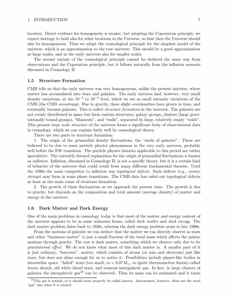
1.5 Structure Formation

CMB tells us that the early universe was very homogeneous, unlike the present universe, wherematter has accumulated into stars and galaxies. The early universe had, however, very smalldensity variations, at the 10−5 to 10−3 level, which we see as small intensity variations of theCMB (the CMB anisotropy). Due to gravity, these slight overdensities have grown in time, andeventually became galaxies. This is called structure formation in the universe. The galaxies arenot evenly distributed in space but form various structures, galaxy groups, clusters (large gravi-tationally bound groups), “filaments”, and “walls”, separated by large, relatively empty “voids”.This present large scale structure of the universe forms a significant body of observational datain cosmology, which we can explain fairly well by cosmological theory.

There are two parts to structure formation:1. The origin of the primordial density fluctuations, the “seeds of galaxies”. These are

believed to be due to some particle physics phenomenon in the very early universe, probablywell before the EW transition. The particle physics theories applicable to this period are ratherspeculative. The currently favored explanation for the origin of primordial fluctuations is knownas inflation. Inflation, discussed in Cosmology II, is not a specific theory, but it is a certain kindof behavior of the universe that could result from many different fundamental theories. Untilthe 1990s the main competitor to inflation was topological defects. Such defects (e.g., cosmic

strings) may form in some phase transitions. The CMB data has ruled out topological defectsat least as the main cause of structure formation.

2. The growth of these fluctuations as we approach the present time. The growth is dueto gravity, but depends on the composition and total amount (average density) of matter andenergy in the universe.

1.6 Dark Matter and Dark Energy

One of the main problems in cosmology today is that most of the matter and energy content ofthe universe appears to be in some unknown forms, called dark matter and dark energy. Thedark matter problem dates back to 1930s, whereas the dark energy problem arose in late 1990s.

From the motions of galaxies we can deduce that the matter we can directly observe as starsand other “luminous matter” is just a small fraction of the total mass which affects the galaxymotions through gravity. The rest is dark matter, something which we observe only due to itsgravitational effect. We do not know what most of this dark matter is. A smaller part of itis just ordinary, “baryonic”, matter, which consists of atoms (or ions and electrons) just likestars, but does not shine enough for us to notice it. Possibilities include planet-like bodies ininterstellar space, “failed” stars (too small, m < 0.07M⊙, to ignite thermonuclear fusion) calledbrown dwarfs, old white dwarf stars, and tenuous intergalactic gas. In fact, in large clusters ofgalaxies the intergalactic gas16 can be observed. Thus its mass can be estimated and it turns

16This gas is ionized, so it should more properly be called plasma. Astronomers, however, often use the word“gas” also when it is ionized.

1 INTRODUCTION 8

out to be several times larger than the total mass of the stars in the galaxies. We can infer thatother parts of the universe, where this gas is too thin to be observable from here, also containsignificant amounts of it; so this is apparently the main component of baryonic dark matter

(BDM). However, there is not nearly enough of it to explain the dark matter problem.Beyond these mass estimates, there are more fundamental reasons (BBN, structure forma-

tion) why baryonic dark matter cannot be the main component of dark matter. Most of thedark matter must be non-baryonic, meaning that it is not made out of protons and neutrons17.The only non-baryonic particles in the standard model of particle physics that could act as darkmatter, are neutrinos. If neutrinos had a suitable mass, ∼ 1 eV, the neutrinos left from theearly universe would have a sufficient total mass to be a significant dark matter component.However, structure formation in the universe requires most of the dark matter to have differentproperties than neutrinos have. Technically, most of the dark matter must be “cold”, instead of“hot”. These are terms that just refer to the dynamics of the particles making up the matter,and do not further specify the nature of these particles. The difference between hot dark matter

(HDM) and cold dark matter (CDM) is that HDM is made of particles whose velocities werelarge compared to escape velocities from the gravity of overdensities, when structure formationbegan, but CDM particles had small velocities. Neutrinos with m ∼ 1 eV, would be HDM. Anintermediate case is called warm dark matter (WDM). Structure formation requires that most ofthe dark matter is CDM, or possibly WDM, but the standard model of particle physics containsno suitable particles. Thus it appears that most of the matter in the universe is made out ofsome unknown particles.

Fortunately, particle physicists have independently come to the conclusion that the standardmodel is not the final word in particle physics, but needs to be “extended”. The proposedextensions to the standard model contain many suitable CDM particle candidates (e.g., neu-tralinos, axions). Their interactions with standard model particles would have to be rather weakto explain why they have not been detected so far. Since these extensions were not invented toexplain dark matter, but were strongly motivated by particle physics reasons, the cosmologicalevidence for dark matter is good, rather than bad, news from a particle physics viewpoint.

In these days the term ”dark matter” usually refers to the nonbaryonic dark matter, andoften excludes also neutrinos, so that it refers only to the unknown particles that are not partof the standard model of particle physics.

Since all the cosmological evidence for CDM comes from its gravitational effects, it has beensuggested by some that it does not exist, and that these gravitational effects might instead beexplained by suitably modifying the law of gravity at large distances. However, the suggestedmodifications do not appear very convincing, and the evidence is in favor of the CDM hypothesis.The gravitational effect of CDM has a role at many different levels in the history and structureof the universe, so it is difficult for a competing theory to explain all of them. Most cosmologistsconsider the existence of CDM as an established fact, and are just waiting for the eventualdiscovery of the CDM particle in the laboratory (perhaps produced with the Large HadronicCollider (LHC) at CERN).18

The situation with the so-called dark energy is different. While dark matter fits well intotheoretical expectations, the status of dark energy is much more obscure. The accumulation ofastronomical data relevant to cosmology has made it possible to determine the geometry andexpansion history of the universe accurately. It looks like yet another component to the energydensity of the universe is required to make everything fit, in particular to explain the observedacceleration of the expansion. This component is called “dark energy”. Unlike dark matter,

17And electrons. Although technically electrons are not baryons (they are leptons), cosmologists refer to mattermade out of protons, electrons, and neutrons as “baryonic”. The electrons are anyway so light, that most of themass comes from the true baryons, protons and neutrons.

18By 2017, it is already a disappointment that LHC has not yet found a dark matter particle.

1 INTRODUCTION 9

Figure 2: Our past light cone.

which is clustered, the dark energy should be relatively uniform in the observable universe. Andwhile dark matter has negligible pressure, dark energy should have large, but negative pressure.The simplest possibility for dark energy is a cosmological constant or vacuum energy. Unlike darkmatter, dark energy was not anticipated by high-energy-physics theory, and it appears difficultto incorporate it in a natural way. Again, another possible explanation is a modification of thelaw of gravity at large distances. In the dark energy case, this possibility is still being seriouslyconsidered. The difference from dark matter is that there is more theoretical freedom, sincethere are fewer relevant observed facts to explain, and that the various proposed models fordark energy do not appear very natural. A nonzero vacuum energy by itself would be naturalfrom quantum field theory considerations, but the observed energy scale is unnaturally low.

1.7 Observable Universe

The observations relevant to cosmology are mainly astronomical. The speed of light is finite, andtherefore, when we look far away, we also look back in time. The universe has been transparentsince recombination, so more than 99.99% of the history of the universe is out there for us tosee. (See Fig. 2.)

The most important channel of observation is the electromagnetic radiation (light, radiowaves, X-rays, etc.) coming from space. We also observe particles, cosmic rays (protons, elec-trons, nuclei) and neutrinos coming from space. A new channel, opened in 2015 by the firstobservation by LIGO (Laser Interferometer Gravitational-wave Observatory), are gravitationalwaves from space. In addition, the composition of matter in the solar system has cosmologicalsignificance.

1 INTRODUCTION 10

1.7.1 Big bang and the steady-state theory

In the 1950s observational data on cosmology was rather sparse. It consisted mainly of theredshifts of galaxies, which were understood to be due to the expansion of space. At that timethere was still room for different basic theories of cosmology. The main competitors were thesteady-state theory and the Big Bang theory.

The steady-state theory is also known as the theory of continuous creation, since it postulatesthat matter is constantly being created out of nothing, so that the average density of the universestays the same despite the expansion. According to the steady-state theory the universe hasalways existed and will always exist and will always look essentially the same, so that there isno overall evolution.

According to the Big Bang theory, the universe had a beginning at a finite time ago in thepast; the universe started at very high density, and as the universe expands its density goesdown. In the Big Bang theory the universe evolves; it was different in the past, and it keepschanging in the future. The name “Big Bang” was given to this theory by Fred Hoyle, one ofthe advocates of the steady-state theory, to ridicule it. Hoyle preferred the steady-state theoryon philosophical grounds; to him, an eternal universe with no evolution was preferable to anevolving one with a mysterious beginning.

Both theories treated the observed expansion of the universe according to Einstein’s theoryof General Relativity. The steady-state theory added to it a continuous creation of matter,whereas the Big Bang theory “had all the creation in the beginning”.19

The accumulation of further observational data led to the abandonment of the steady-statetheory. These observations were: 1) the cosmic microwave background (predicted by the BigBang theory, problematic for steady-state), 2) the evolution of cosmic radio sources (they weremore powerful in the past, or there were more of them), and 3) the abundances of light elementsand their isotopes (predicted correctly by the Big Bang theory).

By today the evidence has become so compelling that it appears extremely unlikely thatthe Big Bang theory could be wrong in any essential way, and the Big Bang theory has becomethe accepted basic framework, or “paradigm” of cosmology. Thus it has become arcane to talkabout ”Big Bang theory”, when we are just referring to modern cosmology. The term ”BigBang” should be understood as originating from this historical context. Thus it refers to thepresent universe evolving from a completely different early stage: hot, dense, rapidly expandingand cooling, instead of being eternal and unchanging. There are still, of course, many openquestions on the details, and the very beginning is still completely unknown.

1.7.2 Electromagnetic channel

Although the interstellar space is transparent (except for radio waves longer than 100 m, ab-sorbed by interstellar ionized gas, and short-wavelength ultraviolet radiation, absorbed by neu-tral gas), Earth’s atmosphere is opaque except for two wavelength ranges, the optical window

(λ = 300–800 nm), which includes visible light, and the radio window (λ = 1mm–20m). Theatmosphere is partially transparent to infrared radiation, which is absorbed by water moleculesin the air; high altitude and dry air favors infrared astronomy. Accordingly, the traditionalbranches of astronomy are optical astronomy and radio astronomy. Observations at other wave-lengths have become possible only during the past few decades, from space (satellites) or at very

19Thus the steady-state theory postulates a modification to known laws of physics, this continuous creation ofmatter out of nothing. The Big Bang theory, on the other hand, is based only on known laws of physics, but itleads to an evolution which, when extended backwards in time, leads eventually to extreme conditions where theknown laws of physics can not be expected to hold any more. Whether there was “creation” or something elsethere, is beyond the realm of the Big Bang theory. Thus the Big Bang theory can be said to be “incomplete” inthis sense, in contrast to the steady-state theory being complete in covering all of the history of the universe.

1 INTRODUCTION 11

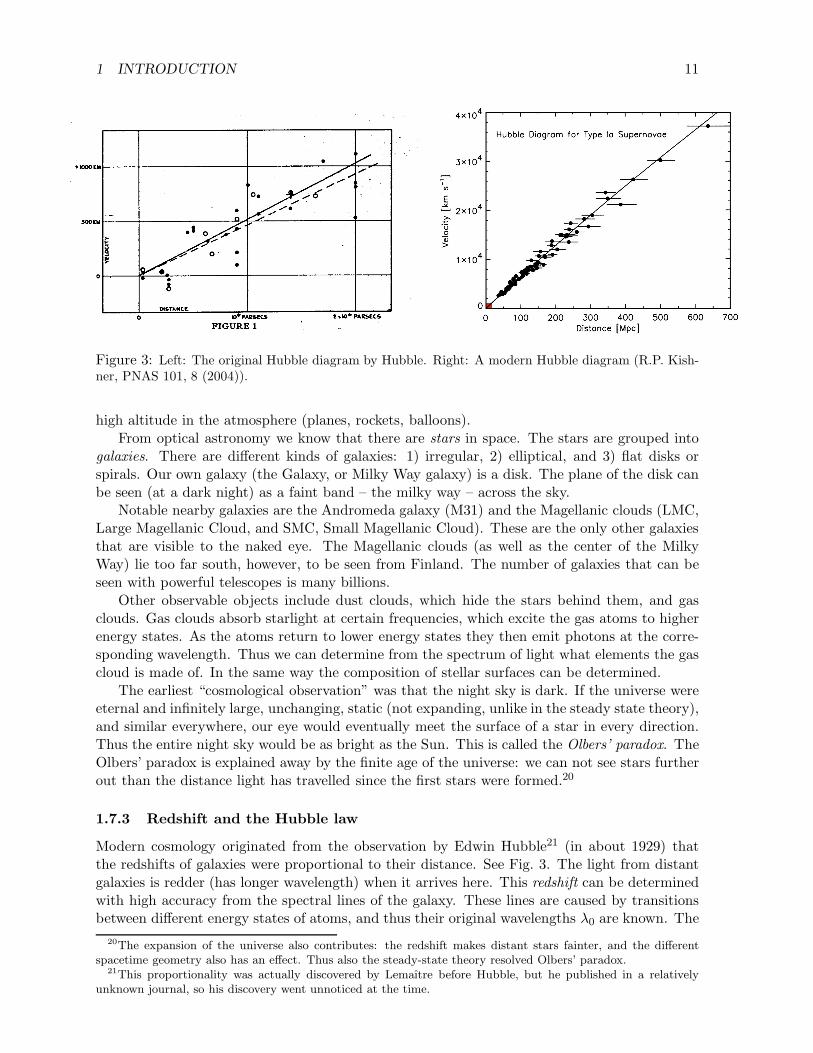
Figure 3: Left: The original Hubble diagram by Hubble. Right: A modern Hubble diagram (R.P. Kish-ner, PNAS 101, 8 (2004)).

high altitude in the atmosphere (planes, rockets, balloons).From optical astronomy we know that there are stars in space. The stars are grouped into

galaxies. There are different kinds of galaxies: 1) irregular, 2) elliptical, and 3) flat disks orspirals. Our own galaxy (the Galaxy, or Milky Way galaxy) is a disk. The plane of the disk canbe seen (at a dark night) as a faint band – the milky way – across the sky.

Notable nearby galaxies are the Andromeda galaxy (M31) and the Magellanic clouds (LMC,Large Magellanic Cloud, and SMC, Small Magellanic Cloud). These are the only other galaxiesthat are visible to the naked eye. The Magellanic clouds (as well as the center of the MilkyWay) lie too far south, however, to be seen from Finland. The number of galaxies that can beseen with powerful telescopes is many billions.

Other observable objects include dust clouds, which hide the stars behind them, and gasclouds. Gas clouds absorb starlight at certain frequencies, which excite the gas atoms to higherenergy states. As the atoms return to lower energy states they then emit photons at the corre-sponding wavelength. Thus we can determine from the spectrum of light what elements the gascloud is made of. In the same way the composition of stellar surfaces can be determined.

The earliest “cosmological observation” was that the night sky is dark. If the universe wereeternal and infinitely large, unchanging, static (not expanding, unlike in the steady state theory),and similar everywhere, our eye would eventually meet the surface of a star in every direction.Thus the entire night sky would be as bright as the Sun. This is called the Olbers’ paradox. TheOlbers’ paradox is explained away by the finite age of the universe: we can not see stars furtherout than the distance light has travelled since the first stars were formed.20

1.7.3 Redshift and the Hubble law

Modern cosmology originated from the observation by Edwin Hubble21 (in about 1929) thatthe redshifts of galaxies were proportional to their distance. See Fig. 3. The light from distantgalaxies is redder (has longer wavelength) when it arrives here. This redshift can be determinedwith high accuracy from the spectral lines of the galaxy. These lines are caused by transitionsbetween different energy states of atoms, and thus their original wavelengths λ0 are known. The

20The expansion of the universe also contributes: the redshift makes distant stars fainter, and the differentspacetime geometry also has an effect. Thus also the steady-state theory resolved Olbers’ paradox.

21This proportionality was actually discovered by Lemaıtre before Hubble, but he published in a relativelyunknown journal, so his discovery went unnoticed at the time.

1 INTRODUCTION 12

redshift z is defined as

z =λ− λ0

λ0

or 1 + z =λ

λ0

(4)

where λ is the observed wavelength. The redshift is observed to be independent of wavelength.The proportionality relation

z = H0d (5)

is called the Hubble law, and the proportionality constant H0 the Hubble constant. Here d is thedistance to the galaxy and z its redshift.

For small redshifts (z ≪ 1) the redshift can be interpreted as the Doppler effect due to therelative motion of the source and the observer. The distant galaxies are thus receding from uswith the velocity

v = z. (6)

The further out they are, the faster they are receding. Astronomers often report the redshift invelocity units (i.e., km/s). Note that 1 km/s = 1/299792.458 = 0.000003356. Since the distancesto galaxies are convenient to give in units of Mpc, the Hubble constant is customarily given inunits of km/s/Mpc, although clearly its dimension is just 1/time or 1/distance.

This is, however, not the proper way to understand the redshift. The galaxies are notactually moving, but the distances between the galaxies are increasing because the intergalacticspace between the galaxies is expanding, in the manner described by general relativity. Weshall later derive the redshift from general relativity. It turns out that equations (5) and (6)hold only at the limit z ≪ 1, and the general result, d(z), relating distance d and redshift zis more complicated (discussed in Chapter 3). In particular, the redshift increases much fasterthan distance for large z, reaching infinity at finite d. However, redshift is directly related tothe expansion. The easiest way to understand the cosmological redshift is that the wavelengthof traveling light expands with the universe. (We derive this result in Chapter 3.) Thus theuniverse has expanded by a factor 1 + z during the time light traveled from an object withredshift z to us.

While the redshift can be determined with high accuracy, it is difficult to determine thedistance d. See Fig. 3, right panel. The distance determinations are usually based on thecosmic distance ladder. This means a series of relative distance determinations between morenearby and faraway objects. The first step of the ladder is made of nearby stars, whose absolutedistance can be determined from their parallax, their apparent motion on the sky due to ourmotion around the Sun. The other steps require “standard candles”, classes of objects with thesame absolute luminosity (radiated power), so that their relative distances are inversely relatedto the square roots of their “brightness” or apparent luminosity (received flux density). Severalsteps are needed, since objects that can be found close by are too faint to be observed from veryfar away.

An important standard candle is a class of variable stars called Cepheids. They are so brightthat they can be observed (with the Hubble Space Telescope) in other galaxies as far away as theVirgo cluster of galaxies, more than 10 Mpc away. There are many Cepheids in the LMC, andthe distance to the LMC (about 50 kpc) is an important step in the distance ladder. For largerdistances supernovae (a particular type of supernovae, called Type Ia) are used as standardcandles.

Errors (inaccuracies) accumulate from step to step, so that cosmological distances, and thusthe value of the Hubble constant, are not known accurately. This uncertainty of distance scaleis reflected in many cosmological quantities. It is customary to give these quantities multipliedby the appropriate power of h, defined by

H0 = h · 100 km/s/Mpc. (7)

1 INTRODUCTION 13

Still in the 1980s different observers reported values ranging from 50 to 100 km/s/Mpc (h = 0.5to 1).22

It was a stated goal of the Hubble Space Telescope (HST) to determine the Hubble constantwith 10% accuracy. As a result of some 10 years of observations the Hubble Space TelescopeKey Project to Measure the Hubble Constant gave as their result in 2001 as [3]

H0 = 72± 8 km/s/Mpc . (8)

Modern observations have narrowed down the range and some recent results are

H0 = 74.0 ± 1.4 km/s/Mpc [4]

H0 = 69.8 ± 1.9 km/s/Mpc [5] (9)

(h = 0.740 ± 0.014 or h = 0.698 ± 0.019). Here the uncertainties (±1.4 and ±1.9) represents a68% confidence range, i.e., it is estimated 68% probable that the true value lies in this range.(Unless otherwise noted, we give uncertainties as 68% confidence ranges. If the probabilitydistribution is the so-called normal (Gaussian) distribution, this corresponds to the standarddeviation (σ) of the distribution, i.e., a 1σ error estimate.) As we see, results from differentobservers are not all entirely consistent, so that the contribution of systematic effects to theprobable error may have been underestimated.23 To single-digit precision, we can use h = 0.7.

The largest observed redshifts of galaxies and quasars are about z ∼ 9. Thus the universehas expanded by a factor of ten while the observed light has been on its way. When the lightleft such a galaxy, the age of the universe was only about 500 million years. At that time thefirst galaxies were just being formed. This upper limit in the observations is, however, not dueto there being no earlier galaxies; such galaxies are just too faint due to both the large distanceand the large redshift. There may well be galaxies with a redshift greater than 10. NASA isbuilding a new space telescope, the James Webb Space Telescope24 (JWST), which would beable to observe these.

The Hubble constant is called a “constant”, since it is constant as a function of position. Itis, however, a function of time, H(t), in the cosmological time scale. H(t) is called the Hubbleparameter, and its present value is called the Hubble constant, H0. In cosmology, it is customaryto denote the present values of quantities with the subscript 0. Thus H0 = H(t0).

The galaxies are not exactly at rest in the expanding space. Each galaxy has its own peculiar

motion vgal, caused by the gravity of nearby mass concentrations (other galaxies). Neighboringgalaxies fall towards each other, orbit each other etc. Thus the redshift of an individual galaxyis the sum of the cosmic and the peculiar redshift.

z = H0d+ n · vgal (when z ≪ 1). (10)

(Here n is the “line-of-sight” unit vector giving the direction from the observer towards thegalaxy.) Usually only the redshift is known precisely. Typically vgal is of the order 500 km/s.(In large galaxy clusters, where galaxies orbit each other, it can be several thousand km/s; butthen one can take the average redshift of the cluster.) For faraway galaxies, H0r ≫ vgal, andthe redshift can be used as a measure of distance. It is also related to the age of the universeat the observed time. Objects with a large z are seen in a younger universe (as the light takesa longer time to travel from this more distant object).

1 INTRODUCTION 14

Figure 4: The distribution of galaxies from the Sloan Digital Sky Survey (SDSS) and the horizon. Weare at the center of this diagram. Each dot represents an observed galaxy. The empty sectors are regionsnot surveyed. The figure shows fewer galaxies further out, since only the brightest galaxies can be seenat large distances. The red color represents the primordial plasma through which we cannot see. Thisfigure can be thought of as our past light cone seen from the “top” (compare to Fig. 2). We see the innersurface of this sphere as the cosmic microwave background (see Fig. 6). As time goes on the horizonrecedes and we can see further out. The “Future comoving visibility limit” is how far one can eventuallysee in the very distant future, assuming the “Concordance Model” for the universe (Sec. 3.3). Becauseof the accelerated expansion of the universe it is not possible to reach the most distant galaxies we see(beyond the circle marked “Unreachable”), even if traveling at (arbitrarily close to) the speed of light.Fig. 5 zooms in to the center region marked with the dotted circle. Figure from Gott et al: “Map of theUniverse” (2005) [2].

1 INTRODUCTION 15

1.7.4 Horizon

Because of the finite speed of light and the finite age of the universe, only a finite part of theuniverse is observable. Our horizon is at that distance from which light has just had time toreach us during the entire age of the universe. Were it not for the expansion of the universe,the distance to this horizon dhor would equal the age of the universe, 14 billion light years (4300Mpc). The expansion complicates the situation; we shall calculate the horizon distance later. Forlarge distances the redshift grows faster than (5). At the horizon z → ∞, i.e., dhor = d(z = ∞).The universe has been transparent only for z < 1090 (after recombination), so the “practicalhorizon”, i.e., the limit to what we can see, lies already at z ∼ 1090. The distances d(z = 1090)and d(z = ∞) are close to each other; z = 4 lies about halfway from here to horizon. Theexpansion of the universe complicates the concept of distance; the statements above refer to thecomoving distance, defined later.

Thus the question of whether the universe is finite or infinite in space is somewhat mean-ingless. In any case we can only observe a finite region, enclosed in the sphere with radiusdhor. Sometimes the word “universe” is used to denote just this observable part of the “whole”universe. Then we can say that the universe contains some 1011 or 1012 galaxies and about1023 stars. Over cosmological time scales the horizon of course recedes and parts of the universewhich are beyond our present horizon become observable. However, if the expansion keeps ac-celerating, as the observations indicate it has been doing already for several billion years, theobservable region is already close to its maximum extent, and in the distant future galaxieswhich are now observable will disappear from our sight due to their increasing redshift.

1.7.5 Optical astronomy and the large scale structure

There is a large body of data relevant to cosmology from optical astronomy. Counting the num-ber of stars and galaxies we can estimate the matter density they contribute to the universe.Counting the number density of galaxies as a function of their distance, we can try to deter-mine whether the geometry of space deviates from Euclidean (as it might, according to generalrelativity). Evolution effects complicate the latter, and this approach never led to conclusiveresults.

From the different redshifts of galaxies within the same galaxy cluster we obtain their relativemotions, which reflect the gravitating mass within the system. The mass estimates for galaxyclusters obtained this way are much larger than those obtained by counting the visible stars andgalaxies in the cluster, pointing to the existence of dark matter.

From the spectral lines of stars and gas clouds we can determine the relative amounts ofdifferent elements and their isotopes in the universe.

The distribution of galaxies in space and their relative velocities tell us about the large scale

structure of the universe. The galaxies are not distributed uniformly. There are galaxy groupsand clusters. Our own galaxy belongs to a small group of galaxies called the Local Group. TheLocal Group consists of three large spiral galaxies: M31 (the Andromeda galaxy), M33 (theTriangulum galaxy25 ; both M31 and M33 are named after the constellations they are locatedin), and the Milky Way, and about 30 smaller (dwarf) galaxies. The nearest large cluster isthe Virgo Cluster. The grouping of galaxies into clusters is not as strong as the grouping ofstars into galaxies. Rather the distribution of galaxies is just uneven; with denser and more

22In fact, there were two “camps” of observers, one reporting values close to 50, the other close to 100, bothclaiming error estimates much smaller than the difference.

23We discuss in Chapter 9 how CMB observations[6] lead to a, model-dependent, smaller value, H0 = 67.4 ±

0.5 km/s/Mpc.24www.jwst.nasa.gov25Sometimes it is called the Pinwheel galaxy, but this name is also being used for M83, M99, and M101.

1 INTRODUCTION 16

Figure 5: The distribution of galaxies from SDSS. This figure shows observed galaxies that are within2 of the equator and closer than 858 Mpc. The empty sectors are regions not surveyed. Figure fromGott et al: ”Map of the Universe” (2005) [2].

1 INTRODUCTION 17

sparse regions. The dense regions can be flat structures (“walls”) which enclose regions with amuch lower galaxy density (“voids”). See Fig. 5. The densest concentrations are called galaxyclusters, but most galaxies are not part of any well defined cluster, where the galaxies orbit thecenter of the cluster.

1.7.6 Radio astronomy

The sky looks very different to radio astronomy. There are many strong radio sources very faraway. These are galaxies which are optically barely observable. They are distributed isotropi-cally, i.e., there are equal numbers of them in every direction, but there is a higher density ofthem far away (at z > 1) than close by (z < 1). The isotropy is evidence of the homogeneityof the universe at the largest scales – there is structure only at smaller scales. The dependenceon distance is a time evolution effect. It shows that the universe is not static or stationary, butevolves with time. Some galaxies are strong radio sources when they are young, but becomeweaker with age by a factor of more than 1000.

Cold gas clouds can be mapped using the 21 cm spectral line of hydrogen. The ground state(n = 1) of hydrogen is split into two very close energy levels depending on whether the protonand electron spins are parallel or antiparallel (the hyperfine structure). The separation of theseenergy levels, the hyperfine structure constant, is 5.9µeV, corresponding to a photon wavelengthof 21 cm, i.e., radio waves. The redshift of this spectral line shows that redshift is independentof wavelength (the same for radio waves and visible light), as it should be according to standardtheory.

1.7.7 Cosmic microwave background

At microwave frequencies the sky is dominated by the cosmic microwave background (CMB),which is highly isotropic, i.e., the microwave sky appears glowing uniformly without any features,unless our detectors are extremely sensitive to small contrasts. The electromagnetic spectrumof the CMB is the black body spectrum with a temperature of T0 = 2.7255 ± 0.0006K [7]. Infact, it follows the theoretical black body spectrum better than anything else we can observe orproduce. There is no other plausible explanation for its origin than that it was produced in theBig Bang. It shows that the universe was homogeneous and in thermal equilibrium at the time(z = 1090) when this radiation originated. The redshift of the photons causes the temperatureof the CMB to fall as (1 + z)−1, so that its original temperature was about T = 3000K.

The state of a system in thermal equilibrium is determined by just a small number of ther-modynamic variables, in this case the temperature and density (or densities, when there areseveral conserved particle numbers). The observed temperature of the CMB and the observeddensity of the present universe allows us to fix the evolution of the temperature and the densityof the universe, which then allows us to calculate the sequence of events during the Big Bang.That the early universe was hot and in thermal equilibrium is a central part of the Big Bangparadigm, and it is often called the Hot Big Bang to spell this out.

With sensitive instruments a small anisotropy can be observed in the microwave sky. Thisis dominated by the dipole anisotropy (one side of the sky is slightly hotter and the other sidecolder), with an amplitude of 3362.1±1.0µK, or ∆T/T0 = 0.001234. This is a Doppler effect dueto the motion of the observer, i.e., the motion of the Solar System with respect to the radiatingmatter at our horizon. The velocity of this motion is v = ∆T/T0 = 369.8 ± 0.1 km/s and it isdirected towards the constellation of Leo (galactic coordinates l = 264.02, b = 48.25; equatorialcoordinates RA 11h11m46s, Dec −657′), near the autumnal equinox (where the ecliptic and theequator cross on the sky) [8]. It is due to two components, the motion of the Sun around thecenter of the Galaxy, and the peculiar motion of the Galaxy due to the gravitational pull of

1 INTRODUCTION 18

Figure 6: The cosmic microwave background. This figure shows the CMB temperature variations overthe entire sky. The color scale shows deviations of −400µK to +400µK from the average temperature of2.7255K. The plane of the milky way is horizontally in the middle. The fuzzy regions are those wherethe CMB is obscured by our galaxy, or nearby galaxies (can you find the LMC?).

1 INTRODUCTION 19

nearby galaxy clusters26.When we subtract the effect of this motion from the observations (and look away from the

plane of the Galaxy – the Milky Way also emits microwave radiation, but with a nonthermalspectrum) the true anisotropy of the CMB remains, with an amplitude of about 3× 10−5, or 80microkelvins.27 See Fig. 6. This anisotropy gives a picture of the small density variations in theearly universe, the “seeds” of galaxies. Theories of structure formation have to match the smallinhomogeneity of the order 10−4 at z ∼ 1090 and the structure observed today (z = 0).

1.8 Distance, luminosity, and magnitude

In astronomy, the radiated power L of an object, e.g., a star or a galaxy, is called its absolute

luminosity. The flux density l (power per unit area) of its radiation here where we observe it,is called its apparent luminosity. Assuming Euclidean geometry, and that the object radiatesisotropically, these are related as

l =L

4πd2, (11)

where d is our distance to the object. For example, the Sun has

L⊙ = 3.9× 1026 W d⊙ = 1.496 × 1011 m l⊙ = 1370W/m2 .

The ancients classified the stars visible to the naked eye into six classes according to theirbrightness. The concept of magnitude in modern astronomy is defined so that it roughly matchesthis ancient classification, but it is a real number, not an integer. The magnitude scale isa logarithmic scale, so that a difference of 5 magnitudes corresponds to a factor of 100 inluminosity. Thus a difference of 1 magnitude corresponds to a factor 1001/5 = 2.512. Theabsolute magnitude M and the apparent magnitude m of an object are defined as

M ≡ −2.5 lgL

L0

m ≡ −2.5 lgl

l0, (12)

where L0 and l0 are reference luminosities (lg ≡ log10). There are actually different magnitudescales corresponding to different regions of the electromagnetic spectrum, with different referenceluminosities. The bolometric magnitude and luminosity refer to the power or flux integrated overall frequencies, whereas the visual magnitude and luminosity refer only to the visible light. Inthe bolometric magnitude scale L0 = 3.0× 1028 W. The reference luminosity l0 for the apparentscale is chosen so in relation to the absolute scale that a star whose distance is d = 10 pc has

26Sometimes it is asked whether there is a contradiction with special relativity here – doesn’t CMB providean absolute reference frame? There is no contradiction. The relativity principle just says that the laws of

physics are the same in the different reference frames. It does not say that systems cannot have reference frameswhich are particularly natural for that system, e.g., the center-of-mass frame or the laboratory frame. For roadtransportation, the surface of the Earth is a natural reference frame. In cosmology, CMB gives us a good “natural”reference frame – it is closely related to the center-of-mass frame of the observable part of the universe, or rather,a part of it which is close to the horizon (the last scattering surface). There is nothing absolute here; the differentparts of the plasma from which the CMB originates are moving with different velocities (part of the 3 × 10−5

anisotropy is due to these velocity variations); we just take the average of what we see. If there is somethingsurprising here, it is that these relative velocities are so small, of the order of just a few km/s; reflecting theastonishing homogeneity of the early universe over large scales. We shall return to the question, whether theseare natural initial conditions, later, when we discuss inflation.

27The numbers refer to the standard deviation of the CMB temperature on the sky. The hottest and coldestspots deviate some 4 or 5 times this amount from the average temperature.

1 INTRODUCTION 20

m = M (exercise: find the value of l0). From this, (11), and (12) follows that the differencebetween the apparent and absolute magnitudes are related to distance as

m−M = −5 + 5 lg d(pc) (13)

This difference is called the distance modulus, and often astronomers just quote the distancemodulus, when they have determined the distance to an object. If two objects are known tohave the same absolute magnitude, but the apparent magnitudes differ by 5, we can concludethat the fainter one is 10 times farther away (assuming Euclidean geometry).

For the Sun we have

M = 4.79 (visual)

M = 4.72 (bolometric)

and (14)

m = −26.78 (visual) ,

where the apparent magnitude is as seen from Earth. Note that the smaller the magnitude, thebrighter the object.

Exercises

The first three exercises are not based on these lecture notes. They should be doable with yourprevious physics background.

Nuclear cosmochronometers. The uranium isotopes 235 and 238 have half-lives t1/2(235) =0.704× 109 a ja t1/2(238) = 4.47× 109 a. The ratio of their abundances on Earth is 235U/238U = 0.00725.When were they equal in abundance? The heavy elements were created in supernova explosions andmixed with the interstellar gas and dust, from which the earth was formed. According to supernovacalculations the uranium isotopes are produced in ratio 235U/238U = 1.3 ± 0.2. What does this tell usabout the age of the Earth and the age of the Universe?

Olbers’ paradox.

1. Assume the universe is infinite, eternal, and unchanging (and has Euclidean geometry). For sim-plicity, assume also that all stars are the same size as the sun, and distributed evenly in space.Show that the line of sight meets the surface of a star in every direction, sooner or later. UseEuclidean geometry.

2. Let’s put in some numbers: The luminosity density of the universe is 108 L⊙/Mpc3 (within a factorof 2). With the above assumption we have then a number density of stars n∗ = 108Mpc−3. Theradius of the sun is r⊙ = 7 × 108m. Define r1/2 so that stars closer than r1/2 cover 50 % of thesky. Calculate r1/2.

3. Let’s assume instead that stars have finite ages: they all appeared t⊙ = 4.6 × 109 a ago. Whatfraction f of the sky do theycover? What is the energy density of starlight in the universe, inkg/m3? (The luminosity, or radiated power, of the sun is L⊙ = 3.85× 1026W).

4. Calculate r1/2 and f for galaxies, using nG = 3× 10−3Mpc−3, rG = 10 kpc, and tG = 1010 a.

Newtonian cosmology. Use Euclidean geometry and Newtonian gravity, so that we interpret theexpansion of the universe as an actual motion of galaxies instead of an expansion of space itself. Considerthus a spherical group of galaxies in otherwise empty space. At a sufficiently large scale you can treat thisas a homogeneous cloud (the galaxies are the cloud particles). Let the mass density of the cloud be ρ(t).Assume that each galaxy moves according to Hubble’s law v(t, r) = H(t)r. The expansion of the cloudslows down due to its own gravity. What is the acceleration as a function of ρ and r ≡ |r|? Express this asan equation for H(t) (here the overdot denotes time derivative). Choose some reference time t = t0 anddefine a(t) ≡ r(t)/r(t0). Show that a(t) is the same function for each galaxy, regardless of the value of

REFERENCES 21

r(t0). Note that ρ(t) = ρ(t0)a(t)−3. Rewrite your differential equation for H(t) as a differential equation

for a(t). You can solve H(t) also using energy conservation. Denote the total energy (kinetic + potential)of a galaxy per unit mass by κ. Show that K ≡ −2κ/r(t0)

2 has the same value for each galaxy, regardlessof the value of r(t0). Relate H(t) to ρ(t0), K, and a(t). Whether the expansion continues forever, orstops and turns into a collapse, depends on how large H is in relation to ρ. Find out the critical valuefor H (corresponding to the escape velocity for the galaxies) separating these two possibilities. Turn therelation around to give the critical density corresponding to a given “Hubble constant” H . What is thiscritical density (in kg/m

3) for H = 70km/s/Mpc?

Practice with natural units.

1. The Planck mass is defined as MPl ≡ 1√8πG

, where G is Newton’s gravitational constant. Give

Planck mass in units of kg, J, eV, K, m−1, and s−1.

2. The energy density of the cosmic microwave background is ργ = π2

15T 4 and its photon density is

nγ = 2

π2 ζ(3)T3, where ζ is Riemann’s zeta function and ζ(3) = 1.20206. What is this energy

density in units of kg/m3 and the photon density in units of m−3, i) today, when T = 2.7255K, ii)when the temperature was T = 1MeV? What was the average photon energy, and what was thewavelength and frequency of such an average photon?

3. Suppose the mass of an average galaxy is mG = 1011 M⊙ and the galaxy density in the universeis nG = 3 × 10−3Mpc−3. What is the galactic contribution to the average mass density of theuniverse, in kg/m3?

4. The critical density for the universe is ρcr0 ≡ 3

8πGH20 , where H0 is the Hubble constant, whose

value we take to be 70 km/s/Mpc. How much is the critical density in units of kg/m3 and inMeV4? What fraction of the critical density is contributed by the microwave background (today),by starlight (see earlier exercise above), and by galaxies?

Reference luminosity. Find the value of l0 for the bolometric scale.

References

[1] Particle Data Group, Review of particle physics, Phys. Rev. D 98, 030001 (2018), p. 128:2. Astrophysical Constants and Parameters

[2] J. Richard Gott III et al., A Map of the Universe, Astrophys. J. 624, 463 (2005), [astro-ph/0310571]

[3] W.L. Freedman et al., Final Results from the Hubble Space Telescope Key Project to Measure

the Hubble Constant, Astrophys. J. 553, 47 (2001)

[4] A.G. Riess et al., Large Magellanic Cloud Cepheid Standards Provide a 1% Foundation

for the Determination of the Hubble Constant and Stronger Evidence for Physics beyond

ΛCDM, Astrophys. J. 876, 85 (2019)

[5] W.L. Freedman et al., The Carnegie-Chicago Hubble Program. VIII. An Independent

Determination of the Hubble Constant Based on the Tip of the Red Giant Branch,arXiv:1907.05922v1 (2019)

[6] Planck Collaboration, Planck 2018 results. VI. Cosmological parameters,arXiv:1807.06209v1 (2018)

[7] D.J. Fixsen, The Temperature of the Cosmic Microwave Background, Astrophys. J. 707,916 (2009)

[8] Planck Collaboration, Planck 2018 results. I. Overview, and the cosmological legacy of

Planck, arXiv:1807.06205v1 (2018)

2 General Relativity

The general theory of relativity (Einstein 1915) is the theory of gravity. General relativity(“Einstein’s theory”) replaced the previous theory of gravity, Newton’s theory. The fundamentalidea in (both special and general) relativity is that space and time form together a 4-dimensionalspacetime. The fundamental idea in general relativity is that gravity is manifested as curvatureof this spacetime. While in Newton’s theory gravity acts directly as a force between two bodies,in Einstein’s theory the gravitational interaction is mediated by the spacetime. A massivebody curves the surrounding spacetime. This curvature then affects the motion of other bodies.“Matter tells spacetime how to curve, spacetime tells matter how to move” [1]. From theviewpoint of general relativity, gravity is not a force at all; if there are no (other) forces (thangravity) acting on a body, we say the body is in free fall. A freely falling body is moving asstraight as possible in the curved spacetime, along a geodesic line. If there are (other) forces,they cause the body to deviate from the geodesic line. It is important to remember that theviewpoint is that of spacetime, not just space. For example, the orbit of Earth around the Sunis curved in space, but as straight as possible in spacetime.

If a spacetime is not curved, we say it is flat, which just means that it has the geometry ofMinkowski space (note the possibly confusing terminology: it is conventional to say “Minkowskispace”, although it is a spacetime). In the case of 2- or 3-dimensional (2D or 3D) space, “flat”means that the geometry is Euclidean.

2.1 Curved 2D and 3D space

If you are familiar with the concept of curved space and how its geometry is given by the metric,you can skip the following discussion of 2- and 3-dimensional spaces and jump to Sec. 2.3.

Ordinary human brains cannot visualize a curved 3-dimensional space, let alone a curved4-dimensional spacetime. However, we can visualize some curved 2-dimensional spaces by con-sidering them embedded in flat 3-dimensional space.1 So let us consider first a 2D space. Imaginethere are 2D beings living in this 2D space. They have no access to a third dimension. Howcan they determine whether the space they live in is curved? By examining whether the laws ofEuclidean geometry hold. If the space is flat, then the sum of the angles of any triangle is 180,and the circumference of any circle with radius r is 2πr. If by measurement they find that thisdoes not hold for some triangles or circles, then they can conclude that the space is curved.

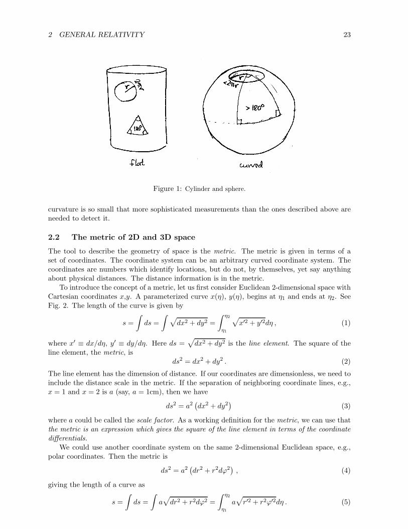
A simple example of a curved 2D space is the sphere. The sum of angles of any triangle ona sphere is greater than 180, and the circumference of any circle is less than 2πr. Straight, i.e.,geodesic, lines, e.g., sides of a triangle, on the sphere are sections of great circles, which dividethe sphere into two equal hemispheres. The radius of a circle is measured along the spheresurface. See Fig. 1.

Note that the surface of a cylinder has Euclidean geometry, i.e., there is no way that 2Dbeings living on it could conclude that it differs from a flat surface, and thus by our definition itis a flat 2D space. (Except that by traveling around the cylinder they could conclude that theirspace has a strange topology).

In a similar manner we could try to determine whether the 3D space around us is curved,by measuring whether the sum of angles of a triangle is 180 or whether a sphere with radius rhas surface area 4πr2. In fact, the space around Earth is curved due to Earth’s gravity, but the

1This embedding is only an aid in visualization. A curved 2D space is defined completely in terms of its 2independent coordinates, without any reference to a higher dimension, the geometry being given by the metric (apart of the definition of the 2D space), an expression in terms of these coordinates. Some such curved 2D spaceshave the same geometry as some 2D surface in flat 3D space. We then say that the 2D space can be embeddedin flat 3D space. But other curved 2D spaces have no such corresponding surface, i.e., they can not be embeddedin flat 3D space.

22

2 GENERAL RELATIVITY 23

Figure 1: Cylinder and sphere.

curvature is so small that more sophisticated measurements than the ones described above areneeded to detect it.

2.2 The metric of 2D and 3D space

The tool to describe the geometry of space is the metric. The metric is given in terms of aset of coordinates. The coordinate system can be an arbitrary curved coordinate system. Thecoordinates are numbers which identify locations, but do not, by themselves, yet say anythingabout physical distances. The distance information is in the metric.

To introduce the concept of a metric, let us first consider Euclidean 2-dimensional space withCartesian coordinates x,y. A parameterized curve x(η), y(η), begins at η1 and ends at η2. SeeFig. 2. The length of the curve is given by

s =

∫

ds =

∫

√

dx2 + dy2 =

∫ η2

η1

√

x′2 + y′2dη , (1)

where x′ ≡ dx/dη, y′ ≡ dy/dη. Here ds =√

dx2 + dy2 is the line element. The square of theline element, the metric, is

ds2 = dx2 + dy2 . (2)

The line element has the dimension of distance. If our coordinates are dimensionless, we need toinclude the distance scale in the metric. If the separation of neighboring coordinate lines, e.g.,x = 1 and x = 2 is a (say, a = 1cm), then we have

ds2 = a2(

dx2 + dy2)

(3)

where a could be called the scale factor. As a working definition for the metric, we can use thatthe metric is an expression which gives the square of the line element in terms of the coordinate

differentials.

We could use another coordinate system on the same 2-dimensional Euclidean space, e.g.,polar coordinates. Then the metric is

ds2 = a2(

dr2 + r2dϕ2)

, (4)

giving the length of a curve as

s =

∫

ds =

∫

a√

dr2 + r2dϕ2 =

∫ η2

η1

a√

r′2 + r2ϕ′2dη . (5)

2 GENERAL RELATIVITY 24

Figure 2: A parameterized curve in Euclidean 2D space with Cartesian coordinates.

Figure 3: Left: A parameterized curve on a 2D sphere with spherical coordinates. Right: The part ofthe sphere covered by the coordinates in Eq. (10).

In a similar manner, in 3-dimensional Euclidean space, the metric is

ds2 = dx2 + dy2 + dz2 (6)

in (dimensionful) Cartesian coordinates, and

ds2 = dr2 + r2dϑ2 + r2 sin2 ϑdϕ2 (7)

in spherical coordinates (where the r coordinate has the dimension of distance, but the angularcoordinates ϑ and ϕ are of course dimensionless).

Now we can go to our first example of a curved (2-dimensional) space, the sphere (the 2-sphere). Let the radius of the sphere be a. For the two coordinates on this 2D space we can takethe angles ϑ and ϕ. We get the metric from the Euclidean 3D metric in spherical coordinatesby setting r ≡ a,

ds2 = a2(

dϑ2 + sin2 ϑdϕ2)

. (8)

The length of a curve ϑ(η), ϕ(η) on this sphere (see Fig. 3) is given by

s =

∫

ds =

∫ η2

η1

a

√

ϑ′2 + sin2 ϑϕ′2dη . (9)

2 GENERAL RELATIVITY 25

Figure 4: The light cone.

For later application in cosmology, it is instructive to now consider a coordinate transforma-tion r = sinϑ (this new coordinate r has nothing to do with the earlier r of 3D space, it is acoordinate on the sphere growing in the same direction as ϑ, starting at r = 0 from the NorthPole (ϑ = 0)). Since now dr = cos ϑdϑ =

√1− r2dϑ, the metric becomes

ds2 = a2(

dr2

1− r2+ r2dϕ2

)

. (10)

For r ≪ 1 (in the vicinity of the North Pole), this metric is approximately the same as Eq. (4),i.e., it becomes polar coordinates on the “Arctic plain”, with scale factor a. Only as r getslarger we begin to notice the deviation from flat geometry. Note that we run into a problemwhen r = 1. This corresponds to ϑ = π/2 = 90, i.e. the “equator”. After this r = sinϑbegins to decrease again, repeating the same values. Also, at r = 1, the 1/(1 − r2) factor inthe metric becomes infinite. We say we have a coordinate singularity at the equator. There isnothing wrong with the space itself, but our chosen coordinate system applies only for a part ofthis space, the region “north” of the equator.

2.3 4D flat spacetime

Let us now return to the 4-dimensional spacetime. The coordinates of the 4-dimensional space-time are (x0, x1, x2, x3), where x0 is a time coordinate (the 0, 1, 2, 3 here are indices, notexponents). Some examples are “Cartesian” (t, x, y, z) and spherical (t, r, ϑ, ϕ) coordinates.The coordinate system can be an arbitrary curved coordinate system. The coordinates do not,by themselves, yet say anything about physical distances. The distance information is in themetric. A Greek index is used to denote an arbitrary spacetime coordinate, xµ, where it isunderstood that µ can have any of the values 0, 1, 2, 3. Latin indices are used to denote spacecoordinates, xi, where it is understood that i can have any of the values 1, 2, 3.

The metric of the Minkowski space of special relativity is

ds2 = −dt2 + dx2 + dy2 + dz2, (11)

in Cartesian coordinates. In spherical coordinates it is

ds2 = −dt2 + dr2 + r2dϑ2 + r2 sin2 ϑ dϕ2, (12)

2 GENERAL RELATIVITY 26

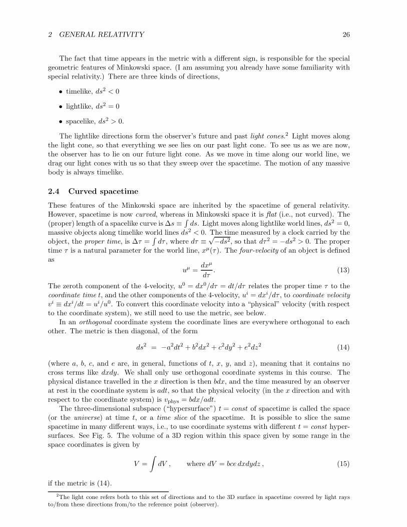
The fact that time appears in the metric with a different sign, is responsible for the specialgeometric features of Minkowski space. (I am assuming you already have some familiarity withspecial relativity.) There are three kinds of directions,

• timelike, ds2 < 0

• lightlike, ds2 = 0

• spacelike, ds2 > 0.

The lightlike directions form the observer’s future and past light cones.2 Light moves alongthe light cone, so that everything we see lies on our past light cone. To see us as we are now,the observer has to lie on our future light cone. As we move in time along our world line, wedrag our light cones with us so that they sweep over the spacetime. The motion of any massivebody is always timelike.

2.4 Curved spacetime

These features of the Minkowski space are inherited by the spacetime of general relativity.However, spacetime is now curved, whereas in Minkowski space it is flat (i.e., not curved). The(proper) length of a spacelike curve is ∆s ≡

∫

ds. Light moves along lightlike world lines, ds2 = 0,massive objects along timelike world lines ds2 < 0. The time measured by a clock carried by theobject, the proper time, is ∆τ =

∫

dτ , where dτ ≡√−ds2, so that dτ2 = −ds2 > 0. The proper

time τ is a natural parameter for the world line, xµ(τ). The four-velocity of an object is definedas

uµ =dxµ

dτ. (13)

The zeroth component of the 4-velocity, u0 = dx0/dτ = dt/dτ relates the proper time τ to thecoordinate time t, and the other components of the 4-velocity, ui = dxi/dτ , to coordinate velocity

vi ≡ dxi/dt = ui/u0. To convert this coordinate velocity into a “physical” velocity (with respectto the coordinate system), we still need to use the metric, see below.

In an orthogonal coordinate system the coordinate lines are everywhere orthogonal to eachother. The metric is then diagonal, of the form

ds2 = −a2dt2 + b2dx2 + c2dy2 + e2dz2 (14)

(where a, b, c, and e are, in general, functions of t, x, y, and z), meaning that it contains nocross terms like dxdy. We shall only use orthogonal coordinate systems in this course. Thephysical distance travelled in the x direction is then bdx, and the time measured by an observerat rest in the coordinate system is adt, so that the physical velocity (in the x direction and withrespect to the coordinate system) is vphys = bdx/adt.

The three-dimensional subspace (“hypersurface”) t = const of spacetime is called the space(or the universe) at time t, or a time slice of the spacetime. It is possible to slice the samespacetime in many different ways, i.e., to use coordinate systems with different t = const hyper-surfaces. See Fig. 5. The volume of a 3D region within this space given by some range in thespace coordinates is given by

V =

∫

dV , where dV = bce dxdydz , (15)

if the metric is (14).

2The light cone refers both to this set of directions and to the 3D surface in spacetime covered by light raysto/from these directions from/to the reference point (observer).

REFERENCES 27

Figure 5: Two coordinate systems with different time slicings.

2.5 Einstein equation

The idea that gravitation is curvature of spacetime and the geometry of spacetime can beexpressed with a metric, is only one part of general relativity (GR). To complete the theoryone must give the law that determines this geometry. In GR this is given by the Einsteinequation, which relates the curvature to the distribution of energy. The Einstein equation isdiscussed in Appendix A. For a proper introduction to the Einstein equation one should takethe General Relativity course. One can also invent other metric theories of gravity where theEinstein equation is replaced with something more complicated. General relativity is the simplestpossibility and is supported by observations, except for the dark energy problem. In CosmologyI we will need only the special case of the Einstein equation called the Friedmann equations,introduced in the next chapter.

References

[1] C.W. Misner, K.S. Thorne, J.A. Wheeler, Gravitation (Freeman 1973)

3 Friedmann–Robertson–Walker Universe

3.1 Kinematics

3.1.1 Robertson–Walker metric

We adopt now the cosmological principle, and discuss the homogeneous and isotropic modelfor the universe. This is called the Friedmann–Robertson–Walker (FRW) or the Friedmann–Lemaıtre–Robertson–Walker universe. Here the homogeneity refers to spatial homogeneity only,so that the universe will still be different at different times.

Spatial homogeneity means that there exists a coordinate system whose t = const hyper-surfaces are homogeneous. This time coordinate is called the cosmic time. Thus the spatialhomogeneity property selects a preferred slicing of the spacetime, reintroducing a separationbetween space and time.

There is good evidence, that the Universe is indeed rather homogeneous (all places lookthe same) and isotropic (all directions look the same) at sufficiently large scales (i.e., ignoringsmaller scale features), larger than 100 Mpc. (Recall the discussion of the cosmological principlein Chapter 1.)

Homogeneity and isotropy mean that the curvature of spacetime must be the same every-where and into every space direction, but it may change in time.1 It can be shown that themetric can then be given (by a suitable choice of the coordinates) in the form

ds2 = −dt2 + a2(t)

[dr2

1−Kr2+ r2dϑ2 + r2 sin2 ϑ dϕ2

]

, (1)

the Robertson–Walker (RW) metric in spherical coordinates. Doing a coordinate transformationwe can also write it in Cartesian coordinates (exercise) :

ds2 = −dt2 + a2(t)dx2 + dy2 + dz2

[1 + 1

4K (x2 + y2 + z2)]2 , (2)

where x = r sinϑ cosϕ, y = r sinϑ sinϕ, z = r cosϑ, and r = (1 −√1−Kr2)/(12Kr). Usually

the spherical coordinates are more useful.This is thus the metric of our universe, to first approximation, and we shall work with this

metric for a large part of this course.2 The time coordinate t is the cosmic time. Here K is aconstant, related to curvature of space, and a(t) is a function of time, related to expansion (orpossible contraction) of the universe. We call

Rcurv ≡ a(t)/√

|K| (3)

the curvature radius of space (at time t).The time-dependent factor a(t) is called the scale factor. When the Einstein equation is

applied to the RW metric, we will get the Friedmann equations, from which we can solve a(t).

1If we drop the condition of isotropy, there are several different possible cosmological models. These spatiallyhomogeneous but anisotropic models are called Bianchi models, after the Bianchi classification. There are nineclasses, Bianchi I–IX, some of them with subclasses. The simplest is Bianchi I, where the geometry of the 3Duniverse is flat, but it expands at different rates in different directions. There is no evidence to favor any Bianchimodel over the FRW. The FRW models are special cases of the Bianchi models, the limit where their anisotropygoes to zero; so cosmological observations can be applied to the Bianchi models to put upper limits to theanisotropy.

2That is, for the whole of Cosmology I. In Cosmology II we shall consider deviations from this homogeneity.

28

3 FRIEDMANN–ROBERTSON–WALKER UNIVERSE 29

This will be done in Sec. 3.2.3 For now, a(t) is an arbitrary function of the time coordinate t.However, for much of the following discussion, we will assume that a(t) grows with time; andwhen we refer to the age of the universe, we assume that a(t) becomes zero at some finite past,which we take as the origin of the time coordinate, t = 0.

We use the dot, ˙≡ d/dt, to denote derivatives with respect to cosmic time t and define

H ≡ a/a . (4)

This quantity H = H(t) gives the expansion rate of the universe, and it is called the Hubble

parameter. Its present value H0 is the Hubble constant. (In cosmology it is customary todenote the present values of quantities with the subscript 0.) The dimension of H is 1/time (orvelocity/distance). In time dt a distance gets stretched by a factor 1+Hdt (a distance L growswith velocity HL).

Note that although the metric describes a homogeneous universe, the metric itself is notexplicitly homogeneous, because it depends also on the coordinate system in addition to thegeometry. (This is a common situation, just like the spherical coordinates of a sphere do notform a homogeneous coordinate system, although the sphere itself is homogeneous.) However,any physical quantities that we calculate from the metric are homogeneous and isotropic.

We notice immediately that the 2-dimensional surfaces t = r = const have the metric of asphere with radius ar. Since the universe is homogeneous, the location of the origin (r = 0) inspace can be chosen freely. We naturally tend to put ourselves at the origin, but for calculationsthis freedom may be useful.

We have the freedom to rescale the radial coordinate r. For example, we can multiply allvalues of r by a factor of 2, if we also divide a by a factor of 2 and K by a factor of 4. Thegeometry of the spacetime stays the same, just the meaning of the coordinate r has changed:the point that had a given value of r has now twice that value in the rescaled coordinate system.There are two common ways to rescale:

1. If K 6= 0, we can rescale r to make K equal to ±1. In this case K is usually denoted k,and it has three possible values, k = −1, 0,+1. In this case r is dimensionless, and a(t) hasthe dimension of distance. For k = ±1, a(t) becomes equal to Rcurv and is often denotedR(t). Equations in this convention will be written in blue.

2. The other way is to rescale a to be one at present4, a(t0) ≡ a0 = 1. In this case a(t) isdimensionless, whereas r and K−1/2 have the dimension of distance. We will adopt thisconvention from Sec. 3.1.4 on.

Choosing one of these two scalings will simplify some of our equations. One must be careful aboutthe possible confusion resulting from comparing equations using different scaling conventions.

IfK = 0, the space part (t = const) of the Robertson–Walker metric is flat. The 3-metric (thespace part of the full metric) is that of ordinary Euclidean space written in spherical coordinates,with the radial distance given by ar. The spacetime, however, is curved, since a(t) depends ontime, describing the expansion or contraction of space. In common terminology, we say the“universe is flat” in this case.

If K > 0, the coordinate system is singular at r = 1/√K. (Remember our discussion of the

2-sphere!) With the substitution (coordinate transformation) r = K−1/2 sin(K1/2χ) the metric

3I have adopted from Syksy the separation of this chapter into Kinematics (Sec. 3.1: RW metric only) andDynamics (Sec. 3.2: RW metric + Friedmann equations). This has the advantage that this Kinematics sectionapplies also to other metric theories of gravity than general relativity, which one may want to consider at somepoint.

4In some discussions of the early universe, it may also be convenient to rescale a to be one at some particularearly time.

3 FRIEDMANN–ROBERTSON–WALKER UNIVERSE 30

Figure 1: The hypersphere. This figure is for K = k = 1. Consider the semicircle in the figure. Itcorresponds to χ ranging from 0 to π. You get the (2-dimensional) sphere by rotating this semicircleoff the paper around the vertical axis by an angle ∆ϕ = 2π. You get the (3-dimensional) hypersphereby rotating it twice, in two extra dimensions, by ∆ϑ = π and by ∆ϕ = 2π, so that each point makesa sphere. Thus each point in the semicircle corresponds to a full sphere with coordinates ϑ and ϕ, andradius (a/

√K) sinχ.

becomes

ds2 = −dt2 + a2(t)[

dχ2 +K−1 sin2(K1/2χ) dϑ2 +K−1 sin2(K1/2χ) sin2 ϑ dϕ2]

. (5)

With the scaling choice K = k = 1 this simplifies to

ds2 = −dt2 + a2(t)[dχ2 + sin2 χdϑ2 + sin2 χ sin2 ϑ dϕ2

]. (6)

The space part has the metric of a hypersphere (a 3-sphere), a sphere with one extra dimension.√Kχ is a new angular coordinate, whose values range over 0–π, just like ϑ. The singularity at

r = 1/√K disappears in this coordinate transformation, showing that it was just a coordinate

singularity, not a singularity of the spacetime. The original coordinates covered only half of thehypersphere, as the coordinate singularity r = 1/

√K divides the hypersphere into two halves.

The case K > 0 corresponds to a closed universe, whose (spatial) curvature is positive.5 This isa finite universe, with circumference 2πa/

√K = 2πRcurv and volume 2π2K−3/2a3 = 2π2R3

curv,and we can think of Rcurv as the radius of the hypersphere.

If K < 0, we do not have a coordinate singularity, and r can range from 0 to ∞. Thesubstitution r = |K|−1/2 sinh(|K|1/2χ) is, however, often useful in calculations. The case K < 0corresponds to an open universe, whose (spatial) curvature is negative. The metric is then

ds2 = −dt2 + a2(t)[

dχ2 + |K|−1 sinh2(|K|1/2χ)(dϑ2 + sin2 ϑ dϕ2

)]

. (7)

This universe is infinite, just like the case K = 0.

5Positive (negative) curvature means that the sum of angles of any triangle is greater than (less than) 180

and that the area of a sphere with radius χ is less than (greater than) 4πχ2.

3 FRIEDMANN–ROBERTSON–WALKER UNIVERSE 31

To handle all three curvature cases simultaneously, we define

fK(χ) ≡

K−1/2 sin(K1/2χ) , (K > 0)

χ , (K = 0)

|K|−1/2 sinh(|K|1/2χ) , (K < 0)

(8)

which allows us to write the RW metric as

ds2 = −dt2 + a2(t)

[

dχ2 + f2K(χ)(dϑ2 + sin2 ϑ dϕ2

)]

, (9)

The RW metric (at a given time) has two associated length scales. The first is the curvatureradius, Rcurv ≡ a|K|−1/2. The second is given by the time scale of the expansion, the Hubble

time or Hubble length tH ≡ lH ≡ H−1, whose present value is

H−10 = 9.7781h−1 Gyr = 2997.92458h−1 Mpc . (10)

(Note that due to the definition of h, the digits 2997.92458 is just the speed of light in units of100 km/s, which makes this value of lH easy to remember.) In the case K = 0 the universe isflat, so the only length scale is the Hubble length.

The coordinates (t, r, ϑ, ϕ) or (t, x, y, z) of the RW metric are called comoving coordinates.This means that the coordinate system follows the expansion of space, so that the space coor-dinates of objects which do not move remain the same. The homogeneity of the universe fixes aspecial frame of reference, the cosmic rest frame given by the above coordinate system, so that,unlike in special relativity, the concept “does not move” has a specific meaning. The coordinatedistance between two such objects stays the same, but the physical, or proper distance betweenthem grows with time as space expands. The time coordinate t, the cosmic time, gives the timemeasured by such an observer at rest, at (r, ϑ, ϕ) = const .

It can be shown that the expansion causes the motion of an object in free fall to slow downwith respect to the comoving coordinate system. For nonrelativistic physical velocities v,

v(t2) =a(t1)

a(t2)v(t1). (11)

The peculiar velocity of a galaxy is its velocity with respect to the comoving coordinate system.

3.1.2 Redshift

Let us now ignore the peculiar velocities of galaxies (i.e., we assume they are = 0), so that theywill stay at fixed coordinate values (r, ϑ, ϕ), and find how their observed redshift z arises. Weset the origin of our coordinate system at galaxy O (observer). Let the r-coordinate of galaxyA be rA. Since we assumed the peculiar velocity of galaxy A to be 0, the coordinate rA staysconstant with time.

Light leaves the galaxy at time t1 with wavelength λ1 and arrives at galaxy O at time t2with wavelength λ2. It takes a time δt1 = λ1/c = 1/ν1 to send one wavelength and a timeδt2 = λ2/c = 1/ν2 to receive one wavelength (ν1 and ν2 are the frequencies, sent and receivedwaves per time). Follow now the two light rays sent at times t1 and t1 + δt1 (see figure). Alongthe light rays t and r change, ϑ and ϕ stay constant (this is clear from the symmetry of theproblem). Light obeys the lightlike condition

ds2 = 0 . (12)

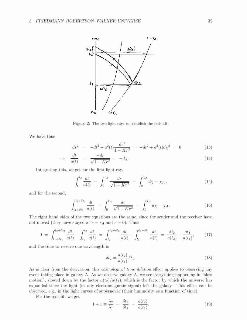
3 FRIEDMANN–ROBERTSON–WALKER UNIVERSE 32

Figure 2: The two light rays to establish the redshift.

We have thus

ds2 = −dt2 + a2(t)dr2

1−Kr2= −dt2 + a2(t)dχ2 = 0 (13)

⇒ dt

a(t)=

−dr√1−Kr2

= −dχ . (14)

Integrating this, we get for the first light ray,

∫ t2

t1

dt

a(t)=

∫ rA

0

dr√1−Kr2

=

∫ χA

0dχ = χA , (15)

and for the second,

∫ t2+δt2

t1+δt1

dt

a(t)=

∫ rA

0

dr√1−Kr2

=

∫ χA

0dχ = χA . (16)

The right hand sides of the two equations are the same, since the sender and the receiver havenot moved (they have stayed at r = rA and r = 0). Thus

0 =

∫ t2+δt2

t1+δt1

dt

a(t)−∫ t2

t1

dt

a(t)=

∫ t2+δt2

t2

dt

a(t)−∫ t1+δt1

t1

dt

a(t)=

δt2a(t2)

− δt1a(t1)

, (17)

and the time to receive one wavelength is

δt2 =a(t2)

a(t1)δt1. (18)

As is clear from the derivation, this cosmological time dilation effect applies to observing anyevent taking place in galaxy A. As we observe galaxy A, we see everything happening in “slowmotion”, slowed down by the factor a(t2)/a(t1), which is the factor by which the universe hasexpanded since the light (or any electromagnetic signal) left the galaxy. This effect can beobserved, e.g., in the light curves of supernovae (their luminosity as a function of time).

For the redshift we get

1 + z ≡ λ2λ1

=δt2δt1

=a(t2)

a(t1). (19)

3 FRIEDMANN–ROBERTSON–WALKER UNIVERSE 33

The redshift of a galaxy directly tells us how much smaller the universe was when the light leftthe galaxy. The result is easy to remember; the wavelength expands with the universe.

Thus the redshift z is related to the value of a(t) and thus to the time t, the age of theuniverse, when the light left the galaxy. We can thus use a or z as alternative time coordinates.Their relation is

1 + z =a0a

or a =a0

1 + z⇒ da

a= − dz

1 + z⇒ da = − a0dz

(1 + z)2. (20)

Note that while a grows with time, z decreases with time: z = ∞ at a = t = 0 and z = 0 att = t0. (More properly, z is a coordinate on our past light cone, so it corresponds to both a timeand a distance.)

3.1.3 Age-redshift relation

If the observed redshift of a galaxy is z, what was the age of the universe when the light left thegalaxy? Without knowing the function a(t) we cannot answer this and other similar questions,but it is useful to derive general expressions in terms of a(t), z, and H(t). We get

H =1

a

da

dt⇒ dt =

da

aH= − dz

(1 + z)H, (21)

so that the age of the universe at redshift z is

t(z) =

∫ t

0dt′ =

∫ ∞

z

dz′

(1 + z′)H. (22)

and the present age of the universe is

t0 ≡ t(z = 0) =

∫ ∞

0

dz′

(1 + z′)H. (23)

The difference gives the light travel time, i.e., how far in the past we see the galaxy,

t0 − t(z) =

∫ z

0

dz′

(1 + z′)H. (24)

3.1.4 Distance

In cosmology, the typical velocities of observers (with respect to the comoving coordinates) aresmall, v < 1000 km/s, so that we do not have to worry about Lorentz contraction (or about thevelocity-related time dilation) and in the FRW model we can use the cosmic rest frame. Theexpansion of the universe brings, however, other complications to the concept of distance. Dowe mean by the distance to a galaxy how far it is now (longer), how far it was when the observedlight left the galaxy (shorter), or the distance the light has traveled (intermediate)?

The proper distance (or “physical distance”) dp(t) between two objects6 is defined as theirdistance measured along the hypersurface of constant cosmic time t. By comoving distance wemean the proper distance scaled to the present value of the scale factor (or sometimes to someother special time we choose as the reference time). If the objects have no peculiar velocity theircomoving distance at any time is the same as their proper distance today.

6or more generally between two points (r, ϑ,ϕ) on the t = const hypersurface. In relativity, proper length ofan object refers to the length of an object in its rest frame, so the use of the word ‘proper’ in ‘proper distance’ isperhaps proper only when the objects are at rest in the FRW coordinate system. Nevertheless, we define it nowthis way.

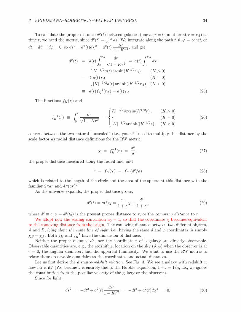
3 FRIEDMANN–ROBERTSON–WALKER UNIVERSE 34

To calculate the proper distance dp(t) between galaxies (one at r = 0, another at r = rA) attime t, we need the metric, since dp(t) =

∫ rA0 ds. We integrate along the path t, ϑ, ϕ = const, or

dt = dϑ = dϕ = 0, so ds2 = a2(t)dχ2 = a2(t) dr2

1−Kr2, and get

dp(t) = a(t)

∫ rA

0

dr√1−Kr2

= a(t)

∫ χA

0dχ

=

K−1/2a(t) arcsin(K1/2rA) (K > 0)

a(t) rA (K = 0)

|K|−1/2a(t) arsinh(|K|1/2rA) (K < 0)

≡ a(t)f−1K (rA) = a(t)χA (25)

The functions fK(χ) and

f−1K (r) ≡

∫ r

0

dr√1−Kr2

=

K−1/2 arcsin(K1/2r) , (K > 0)

r , (K = 0)

|K|−1/2arsinh(|K|1/2r) . (K < 0)

(26)

convert between the two natural “unscaled” (i.e., you still need to multiply this distance by thescale factor a) radial distance definitions for the RW metric:

χ = f−1K (r) =

dp

a, (27)

the proper distance measured along the radial line, and

r = fK(χ) = fK (dp/a) (28)

which is related to the length of the circle and the area of the sphere at this distance with thefamiliar 2πar and 4π(ar)2.

As the universe expands, the proper distance grows,

dp(t) = a(t)χ =a0

1 + zχ ≡ dc

1 + z, (29)

where dc ≡ a0χ = dp(t0) is the present proper distance to r, or the comoving distance to r.We adopt now the scaling convention a0 = 1, so that the coordinate χ becomes equivalent

to the comoving distance from the origin. The comoving distance between two different objects,A and B, lying along the same line of sight, i.e., having the same ϑ and ϕ coordinates, is simplyχB − χA. Both fK and f−1

K have the dimension of distance.Neither the proper distance dp, nor the coordinate r of a galaxy are directly observable.

Observable quantities are, e.g., the redshift z, location on the sky (ϑ,ϕ) when the observer is atr = 0, the angular diameter, and the apparent luminosity. We want to use the RW metric torelate these observable quantities to the coordinates and actual distances.

Let us first derive the distance-redshift relation. See Fig. 3. We see a galaxy with redshift z;how far is it? (We assume z is entirely due to the Hubble expansion, 1+ z = 1/a, i.e., we ignorethe contribution from the peculiar velocity of the galaxy or the observer).

Since for light,

ds2 = −dt2 + a2(t)dr2

1−Kr2= −dt2 + a2(t)dχ2 = 0, (30)

3 FRIEDMANN–ROBERTSON–WALKER UNIVERSE 35

Figure 3: Calculation of the distance-redshift relation.

we have

dt = −a(t) dr√1−Kr2

= −a(t)dχ ⇒∫ t0

t1

dt

a(t)=

∫ r

0

dr√1−Kr2

= χ = dc . (31)

The comoving distance to redshift z is thus

dc(z) = χ(z) =

∫ t0

t1

dt

a(t)=

∫ 1

11+z

da

a

1

da/dt=

∫ z

0

dz′

H(z′). (32)

The proper distance at the time the light left the galaxy is

dp(z) =1

1 + z

∫ z

0

dz′

H(z′). (33)

The “distance light has traveled” (i.e., adding up the infinitesimal distances measured by asequence of observers at rest along the light path) is equal to the light travel time, Eq. (24). Ina monotonously expanding (or contracting) universe it is intermediate between dp(z) and dc(z).

We encounter the beginning of time, t = 0, at a = 0 or z = ∞. Thus the comoving distancelight has traveled during the entire age of the universe is

dchor = χhor =

∫ ∞

0

dz′

H(z′). (34)

This distance (or the sphere with radius dchor, centered on the observer) is called the horizon,since it represent the maximum distance we can see, or receive any information from.

There are actually several different concepts in cosmology called the horizon. To be exact,the one defined above is the particle horizon. Another horizon concept is the event horizon,which is related to how far light can travel in the future. The Hubble distance H−1 is also oftenreferred to as the horizon (especially when one talks about subhorizon and superhorizon distancescales).

3.1.5 Volume

The objects we observe lie on our past light cone, and the observed quantities are z, ϑ, ϕ, so theseare the observer’s coordinates for the light cone. What is the volume of space correspondingto a range ∆z∆ϑ∆ϕ ? Note that the light cone is a lightlike surface, so its “volume” is zero.Here we mean instead the volume that we get when we project a section of it onto the t =

3 FRIEDMANN–ROBERTSON–WALKER UNIVERSE 36

Figure 4: Defining the angular diameter distance.

const hypersurface crossing this section at a particular z (which is unique when ∆z = dz isinfinitesimal).

From Eq. (33), the proper distance corresponding to dz is dz/[(1 + z)H(z)]. Directly fromthe RW metric, the area corresponding to dϑdϕ is ardϑ× ar sinϑdϕ, so that the proper volumeelement becomes

dV p =a2r2 sinϑ

(1 + z)H(z)dzdϑdϕ =

a2r2

(1 + z)H(z)dzdΩ (35)

and the comoving volume is

dV c = (1 + z)3dV =r2

H(z)dzdΩ . (36)

These are the volume elements for counting the number density or comoving number densityof galaxies from observations. If the number of galaxies is conserved, in a homogeneous universetheir comoving number density should be independent of z. Thus, in principle, from suchobservations one should be able to determineH(z). In practice this is made difficult by evolutionof galaxies with time, mergers of galaxies, and the fact that it is more difficult to observe galaxiesat larger z.

3.1.6 Angular diameter distance

The distance-redshift relation (32) obtained above would be nice if we already knew the functiona(t). We can turn the situation around and use an observed distance-redshift relation, to obtaininformation about a(t), or equivalently, about H(z). But for that we need a different distance-redshift relation, one where the “distance” is replaced by some directly observable quantity.

Astronomers employ various such auxiliary distance concepts, like the angular diameter

distance or the luminosity distance. These would be equal to the true distance in Euclideannon-expanding space.

To answer the question: “what is the physical size s of an object, whom we see at redshiftz subtending an angle ϑ on the sky?” we need the concept of angular diameter distance dA.

In Euclidean geometry (see Fig. 4),

s = ϑd or d =s

ϑ. (37)

Accordingly, we define

dA ≡ sp

ϑ, (38)

where sp was the proper diameter of the object when the light we see left it, and ϑ is the observedangle. For large-scale structures, which expand with the universe, we use the comoving angulardiameter distance dcA ≡ sc/ϑ, where sc = (1 + z)sp is the comoving diameter of the structureand z is its redshift. Thus dcA = (1 + z)dA.

3 FRIEDMANN–ROBERTSON–WALKER UNIVERSE 37

From the RW metric, the physical length sp corresponding to an angle ϑ is, from ds2 =a2(t)r2dϑ2 ⇒ sp = a(t)rϑ. Thus

dA(z) = a(t)r =r

1 + z=

fK(χ)

1 + z=

1

1 + zfK

(∫ 1

1

1+z

da

a

1

da/dt

)

=1

1 + zfK

(∫ z

0

dz′

H(z′)

)

(39)

The comoving angular diameter distance is then

dcA = r = fK

(∫ 1

11+z

da

a

1

da/dt

)

= fK

(∫ z

0

dz′

H(z′)

)

. (40)

For the flat (K = 0) FRW model r = fK(χ) = χ, so that the angular diameter distance isequal to the proper distance when the light left the object and the comoving angular diameterdistance is equal to the comoving distance.

For large distances (redshifts) the angular diameter distance may have the counterintuitiveproperty that after some z it begins to decrease as a function of z. Thus objects with are behindother objects as seen from here will nevertheless have a smaller angular diameter distance. Thereare two reasons for such behavior:

In a closed (K > 0) universe objects which are on the “other side” of the universe (the3-sphere), i.e., with K1/2χ > π/2, will cover a larger angle as seen from here because of thespherical geometry (if we can see this far). This effect comes from the fK in Eq. (39). Anobject at exactly opposite end (K1/2χ = π) would cover the entire sky as light from it wouldreach us from every direction after traveling half-way around the 3-sphere. In our universe thesesituations do not occur in practice, because lower limits to the size of the 3-sphere7 are muchlarger than the distance light has traveled in the age of the Universe.

The second reason, which does apply to the observed universe, and applies only to dA, notto dcA, is the expansion of the universe. An object, which does not expand with the universe,occupied a much larger comoving volume in the smaller universe of the past. This effect is the1/(1+z) factor in Eq. (39), which for large z decreases faster than the other part grows. In otherwords, the physical size of the 2-sphere corresponding to a given redshift z has a maximum atsome finite redshift (of the order z ∼ 1), and for larger redshifts it is again smaller. (The samebehavior applies to the proper distance dp(z).)

Suppose we have a set of standard rulers, objects that we know are all the same size sp,observed at different redshifts. Their observed angular sizes ϑ(z) then give us the observed

angular diameter distance as dA(z) = sp/ϑ(z). This observed function can be used to determinethe expansion history a(t), or H(z).

3.1.7 Luminosity distance

In transparent Euclidean space, an object whose distance is d and whose absolute luminosity(radiated power) is L would have an apparent luminosity l = L/4πd2. Thus we define theluminosity distance of an object as

dL ≡√

L

4πl. (41)

Consider the situation in the RW metric. The absolute luminosity can be expressed as:

L =number of photons emitted

time× their average energy =

NγEem

tem. (42)

7Observations tell us that the curvature of the Universe is very small, so that we have not been able todetermine which of the three geometries applies to it.

3 FRIEDMANN–ROBERTSON–WALKER UNIVERSE 38

If the observer (at present time, a0 = 1) is at a coordinate distance r from the source (notehow we now put the origin of the coordinate system at the source), the photons have at thatdistance spread over an area

A = 4πr2 . (43)

The apparent luminosity can be expressed as:

l =number of photons observed

time · area × their average energy =NγEobs

tobsA. (44)

The number of photons Nγ is conserved, but their energy is redshifted, Eobs = Eem/(1 + z).Also, if the source is at redshift z, it takes a factor 1 + z longer to receive the photons ⇒ tobs =(1 + z)tem. Thus,

l =NγEobs

tobsA=

NγEem

tem

1

(1 + z)21

4πr2. (45)

From Eq. (41),

dL ≡√

L

4πl= (1 + z)r = (1 + z)dcA(z) = (1 + z)2dA(z) . (46)

Compared to the comoving angular diameter distance, dcA(z), we have a factor (1+z), whichcauses dL to increase faster with z than dcA(z). There is one factor of (1 + z)1/2 from photonredshift and another factor of (1 + z)1/2 from cosmological time dilation, both contributingto making large-redshift objects dimmer. When compared to dA(z), there is another factor of(1+z) from the expansion of the universe, which we discussed in Sec. 3.1.6, which causes distantobjects to appear larger on the sky, but does not contribute to their apparent luminosity. Thusthe surface brightness (flux density per solid angle) of objects decreases with redshift as

d2A/d2L = (1 + z)−4 (47)

(flux density l ∝ d−2L , solid angle Ω ∝ d−2

A .)8

Suppose that we have a set of standard candles, objects that we know all have the same L.From their observed redshifts and apparent luminosities we get an observed luminosity-distance-redshift relation dL(z) =

√

L/4πl, which can be used to determine a(t), or H(z).

3.1.8 Hubble law

In Sec. 1 we introduced the Hubble law

z = H0d ⇒ d = H−10 z , (48)

which was based on observations (at small redshifts). Now that we have introduced the differentdistance concepts, dp, dc, dA, d

cA, dL, in an expanding universe, and derived exact formulae (33,

32, 39, 40, 46) for them in the RW metric, we can see that for z ≪ 1 (when we can approximateH(z) = H0) all of them give the Hubble law as an approximation, but all of them deviate fromit, in a different manner, for z ∼ 1 and larger.

8In practical observations there is the additional issue that observations are made in some frequency band(wavelenth range), and different redshifts bring different parts of the spectrum of the object within this band.

3 FRIEDMANN–ROBERTSON–WALKER UNIVERSE 39

3.1.9 Conformal time

In the comoving coordinates of Eqs. (1), (6), and (7), the space part of the coordinate systemis expanding with the expansion of the universe. It is often practical to make a correspondingchange in the time coordinate, so that the “unit of time” (i.e., separation of time coordinatesurfaces) also expands with the universe. The conformal time η is defined by

dη ≡ dt

a(t), or η =

∫ t

0

dt′

a(t′). (49)

The RW metric acquires the form

ds2 = a2(η)

[

−dη2 + dr2

1−Kr2+ r2

(dϑ2 + sin2 ϑ dϕ2

)]

, (50)

or with the other choice of the radial coordinate, χ,

ds2 = a2(η)

[

−dη2 + dχ2 + f2K(χ)(dϑ2 + sin2 ϑ dϕ2

)]

, (51)

The form (51) is especially nice for studying radial (dϑ = dϕ = 0) light propagation, becausethe lightlike condition ds2 = 0 becomes dη = ±dχ. In the end of the calculation one may needto convert conformal time back to cosmic time to express the answer in terms of the latter.

3 FRIEDMANN–ROBERTSON–WALKER UNIVERSE 40

3.2 Dynamics

3.2.1 Friedmann equations

The fundamental equation of general relativity is the Einstein equation, which relates the cur-vature of spacetime to the distribution of matter and energy. When applied to the homogeneousand isotropic case, i.e., the Robertson-Walker metric, it leads9 to the Friedmann equations10

(a

a

)2

+K

a2=

8πG

3ρ (54)

a

a= −4πG

3(ρ+ 3p) . (55)

(“Friedmann equation” in singular refers to Eq. (54).) On the left, we have the curvatureof spacetime, which in the RW metric appears as expansion of space given by H ≡ a/a andcurvature of space given by K/a2. On the right, we have the energy density ρ and pressure p ofmatter/energy. G = 6.674 30 ± 15× 10−11 m3/kgs2 is the gravitational constant, the same as inNewton’s theory of gravity. Homogeneity implies the same density and pressure everywhere, sothat they depend on time alone,

ρ = ρ(t) , p = p(t) . (56)

Using the Hubble parameter

H ≡ a/a ⇒ H =a

a− a2

a2⇒ a

a= H +H2 (57)

we can write the Friedmann equations also as

H2 =8πG

3ρ− K

a2(58)

H = −4πG(ρ + p) +K

a2. (59)

In general relativity, we do not have, in general, conservation of energy or momentum. Thetheoretical physics viewpoint is that conservation laws result from symmetries; energy conserva-tion follows from time-translation symmetry and momentum conservation from space-translationsymmetry. Unless the geometry of spacetime has such symmetries we do not have these con-servation laws. In particular, expansion of the universe breaks time-translation symmetry andtherefore energy is not conserved. The homogeneity of the RW metric leads to a form of mo-mentum conservation, ap = const , for particles moving in this metric.

However, the equivalence principle of general relativity requires that locally (at small scaleswhere we do not notice the curvature of spacetime), energy and momentum are conserved.From this follows a law, called energy-momentum continuity, that applies at all scales. It can

9The Einstein equation and the derivation of the Friedmann equations from it are discussed in Appendix A.10Including the cosmological constant Λ (the simplest possible modification of the Einstein equation, discussed

in Appendix A), these equations take the form

(

a

a

)2

+K

a2−

Λ

3=

8πG

3ρ (52)

a

a−

Λ

3= −

4πG

3(ρ+ 3p) . (53)

We shall not include Λ in these equations. Instead, we allow for the presence of vacuum energy ρvac, which hasthe same effect.

3 FRIEDMANN–ROBERTSON–WALKER UNIVERSE 41

be derived from the Einstein equation. In the present case this becomes the energy continuity

equation

ρ = −3(ρ+ p)a

a. (60)

(Exercise: Derive this from the Friedmann equations!) Since isotropy requires that the fluid isat rest, there is no corresponding equation for its momentum.

The Friedmann equation (58) connects the three quantities, the density ρ, the space curvatureK/a2, and the expansion rate H of the universe,

ρ =3

8πG

(

H2 +K

a2

)

≡ ρcr +3K

8πGa2. (61)

(Note that the curvature quantity K/a2 = 1/R2curv is invariant under the r coordinate scaling

we discussed earlier.) We defined the critical density

ρcr ≡3H2

8πG, (62)

corresponding to a given value of the Hubble parameter.11 The critical density changes in timeas the Hubble parameter evolves. The present value of the critical density is given by the Hubbleconstant as

ρcr0 ≡ ρcr(t0) ≡ 3H20

8πG= 1.878 342 × 10−26h2 kg/m3

= 10.5367h2 GeV/m3 = 2.775 × 1011h2 M⊙/Mpc3 . (63)

The nature of the curvature then depends on the density ρ :

ρ < ρcr ⇒ K < 0 (64)

ρ = ρcr ⇒ K = 0 (65)

ρ > ρcr ⇒ K > 0 . (66)

The density parameter Ω is defined

Ω ≡ ρ

ρcr(67)

(where all three quantities are functions of time). Thus Ω = 1 implies a flat universe, Ω < 1 anopen universe, and Ω > 1 a closed universe. The Friedmann equation can now be written as

Ω = 1 +K

H2a2⇒ Ωk(t) ≡ 1− Ω(t) = − K

H(t)2a(t)2, (68)

a very useful relation. Here K is a constant, and the other quantities are functions of time Ω(t),H(t), and a(t). The two length scales are thus related by

Rcurv =H−1

√

|Ωk(t)|. (69)

Note that if Ω < 1 (or > 1), it will stay that way. And if Ω = 1, it will stay constant, Ω = Ω0 = 1.Observations suggest that the density of the universe today is close to critical, Ω0 ≈ 1, so thatRcurv0 ≫ H−1

0 unless K = 0 (so that Rcurv = ∞). Writing in the present values, (68) gives

Ωk ≡ 1− Ω0 = − K

H20

. (70)

11We could also define likewise a critical Hubble parameter Hc corresponding to a given density ρ, but since,of the above three quantities, the Hubble constant has usually been the best determined observationally, it hasbeen better to refer other quantities to it.

3 FRIEDMANN–ROBERTSON–WALKER UNIVERSE 42

We defined a new notation Ωk to represent the deviation of Ω from 1, due to curvature. Notethat we write just Ωk for its present value (instead of Ωk0); if we mean the time-dependentvalue 1 − Ω, we always write Ωk(t). We adopt this common custom since we will mostly referto the present value, and don’t like to have multiple subscripts there. Note that a positive Ωk

corresponds to negative curvature and vice versa. (This sign convention is so that we have apleasing symmetry in the Friedmann equation, see Sec. 3.2.2, Eqs. 108, 109, 110.)

Newtonian cosmology. Newtonian gravity is known to be a good approximation to general relativityfor many situations, so we should be able to get something like the Friedmann equations from it, too.Consider therefore a large spherically symmetric expanding homogeneous group of galaxies in otherwiseempty Euclidean space. Spherical symmetry implies that all motion is radial. Let r(t) be the radialcoordinate (distance from origin) of some galaxy. The velocity of the galaxy is then r. Denote the totalmass of all galaxies within r by

M(r) ≡ 4π

3r3ρ , (71)

where ρ is the mass density, assumed homogeneous, due to the galaxies. We know that in Newtoniangravity the gravitational force at r due to a spherically symmetric mass distribution is equal to that of apoint mass M(r) located at r = 0 (the force due to the outer masses, beyond r, cancels). Therefore theacceleration of the galaxy is

r = −GM(r)

r2= −4πG

3ρr2 ⇒ r

r= −4πG

3ρ . (72)

Defining H ≡ r/r gives

H +H2 =r

r= −4πG

3ρ . (73)

Choose now a reference time t0, denote r(t0) ≡ r0, and define

a(t) ≡ r(t)

r0⇒ a

a= H(t) (74)

anda

a= −4πG

3ρ(t) . (75)

So far we considered the motion of some individual galaxy. Assume now as an initial condition thatH(t0) = H0 is the same for all galaxies (Hubble law). Since the differential equation (75) and the initialconditions a(t0) = 1 and a(t0) = H0 are the same for all galaxies, the solution a(t) will also be the samefor all galaxies. Therefore no galaxy will move past another and the “mass inside” for any particulargalaxy will stay constant

M(r) =4π

3ρa3r30 = const ⇒ ρ(t) ∝ a−3 . (76)

Thus the mass density decreases homogeneously. (There is an apparent circular argument here, since wealready assumed that ρ in (75) will stay homogenous. But we have now shown that this assumption leadsto a consistent solution; and since the solution must be unique, the assumption must be correct.)

The solution depends on the initial conditions H0 (related to kinetic energy) and ρ0 (related togravitational potential energy). Consider the situation from energy conservation. The total energy of anindividual galaxy is

E = 12mr2 −m

GM(r)

r= 1

2mr2 − 4πG

3mρr2 ≡ mκ = const , (77)

where m is the mass of the galaxy and

κ ≡ 12r2 − 4πG

3ρr2 = 1

2a2r20 −

4πG

3ρa2r20 (78)

is energy/mass. We get that

K ≡ −2κ

r20= −a2 + 8πG

3ρa2 (79)

3 FRIEDMANN–ROBERTSON–WALKER UNIVERSE 43

is the same for all galaxies. Dividing by a2 this energy conservation law becomes the Friedmann equation

(a

a

)2

=8πG

3ρ− K

a2. (80)

Comparing (80) and (75) to (54) and (55) we note that the only apparent difference is that there isno pressure p in (75). This is a difference between Newtonian gravity and general relativity: in generalrelativity also pressure is a source of gravity. Besides this apparent difference there are fundamentalconceptual differences: in the Newtonian description K referred to total (kinetic+potential) energy of agalaxy and the space was Euclidian; in the relativistic description K gives the curvature of space and theconcept of gravitational potential energy does not exist. In the Newtonian description the galaxies aremoving; in the relativistic description the space is expanding. The Newtonian description requires thatthe group of galaxies has an outer boundary, which has to be spherical. If this boundary, beyond whichthere should be no galaxies, is far away, at r ≥ H−1, galaxies there would be moving faster than thespeed of light (with respect to the galaxies at the center). Even in the case where pressure is negligible,so that the “Friedmann” equations are the same, these conceptual differences lead to different physicalresults (e.g., redshift) due to the different spacetime geometry.

To solve the Friedmann equations, we need the equation of state that relates p and ρ. Ingeneral, the pressure p of matter may depend also on other thermodynamic variables than theenergy density ρ. The equation of state is called barotropic if p is uniquely determimed by ρ,i.e., p = p(ρ). Regardless of the nature of matter, in a homogeneous universe we have p = p(ρ)in practice, if the energy density decreases monotonously with time, since p = p(t), ρ = ρ(t) andwe can invert the latter to get t(ρ), so that we can write p = p(t) = p(t(ρ)) ≡ p(ρ).

We define the equation-of-state parameter

w ≡ p

ρ(81)

so that we can formally write the equation of state as

p = wρ , (82)

and the energy continuity equation as

ρ

ρ= −3(1 + w)

a

a⇒ d ln ρ = −3(1 + w)d ln a , (83)

where, in general, w = w(t). Equation (83) can be formally integrated to

ρ

ρ0= exp

∫ 1

a3[1 + w(a′)]

da′

a′

= exp

∫ z

0dz′

3[1 + w(z′)]

1 + z′

. (84)

The simplest case is the one where p ∝ ρ, so that

p = wρ , w = const , (85)

in which case the solution of (83) is

ρ = ρ0a−3(1+w) . (86)

There are three such cases:

• “Matter” (w = 0) (called “matter” in cosmology, but “dust” in general relativity), mean-ing nonrelativistic matter (particle velocities v ≪ 1), for which p≪ ρ, so that we can forgetthe pressure, and approximate p = 0. From Eq. (60), d(ρa3)/dt = 0, or ρ ∝ a−3.

3 FRIEDMANN–ROBERTSON–WALKER UNIVERSE 44

• “Radiation” (w = 1/3), meaning ultrarelativistic matter (where particle energies are≫ their rest masses, which is always true for massless particles like photons), for whichp = ρ/3. From Eq. (60), d(ρa4)/dt = 0, or ρ ∝ a−4.

• Vacuum energy (w = −1) (or the cosmological constant), for which ρ = const (propertyof the vacuum, a fundamental constant). From Eq. (60) follows the equation of state forvacuum energy: p = −ρ. Thus a positive vacuum energy12 corresponds to a negative vac-uum pressure. You may be used to pressure being positive, but there is nothing unphysicalabout negative pressure. In other contexts it is often called (positive) “tension” instead of(negative) “pressure”.13

We know that the Universe contains ordinary, nonrelativistic matter. We also know thatthere is radiation, especially the cosmic microwave background. In Chapter 4 we shall discusshow the different known particle species behave as radiation in the early universe when it is veryhot, but as the universe cools, the massive particles change from ultrarelativistic (radiation) tononrelativistic (matter). During the transition period the pressure due to that particle speciesfalls from p ≈ ρ/3 to p ≈ 0. We shall discuss these transition periods in Chapter 4. In thischapter we focus on the later evolution of the universe (after big bang nucleosynthesis, BBN).Then the known forms of matter and energy in the universe can be divided into these two classes:matter (p ≈ 0) and radiation (p ≈ ρ/3).14

We already revealed in Chapter 1 that the present observational data cannot be explainedin terms of known forms of particles and energy using known laws of physics, and therefore webelieve that there are other, unknown forms of energy in the universe, called “dark matter”and “dark energy”. Dark matter has by definition negligible pressure, so that we can ignore itspressure in the Friedmann equations. However, to explain the observed expansion history of theuniverse, an energy component with negative pressure is needed. This we call dark energy. We donot know its equation of state. The simplest possibility for dark energy is just the cosmologicalconstant (vacuum energy), which fits current data perfectly. Therefore we shall carry on ourdiscussion assuming three energy components: matter, radiation, and vacuum energy. We shalllater (at end of Sec. 3.2.4 and in Cosmology II) comment on how much current observationsactually constrain the equation of state for dark energy.

If the universe contains several energy components

ρ =∑

i

ρi with pi = wiρi (87)

without significant energy transfer between them, then each component satisfies the energycontinuity equation separately,

ρiρi

= −3(1 + wi)a

a. (88)

12In the quantum field theory view, “vacuum” is the minimum energy density state of the system. Therefore anyother contribution to energy density is necessarily positive, but whether the vacuum energy density itself needsto be nonnegative is less clear. Other physics except general relativity is sensitive only to energy differenciesand thus does not care about the value of vacuum energy density. In general relativity it is a source of gravity,but cannot be distinguished from a cosmological constant, which is a modification of the law of gravity by anarbitrary constant that could be negative just as well as positive. For simplicity we will here include the possiblecosmological constant in the concept of vacuum energy, and thus we should allow for negative vacuum energydensity also.

13In Chapter 4 we derive formulae for the pressures of different particle species in thermal equilibrium. Thesealways give a positive pressure. The point is that there we ignore interparticle forces. To make the pressurefrom particles negative would require attractive forces between particles. But the vacuum pressure is not fromparticles, it’s from the vacuum. If the dark energy is not just vacuum energy, it is usually thought to be somekind of field. For fields, a negative pressure comes out more naturally than for particles.

14Except that we do not know the small masses of neutrinos. Depending on the values of these masses, neutrinosmay make this radiation-to-matter transition sometime during this “later evolution”.

3 FRIEDMANN–ROBERTSON–WALKER UNIVERSE 45

and, if wi = const ,ρi ∝ a−3(1+wi) ⇒ ρi = ρi0a

−3(1+wi) . (89)

In the early universe there were times where such energy transfer was important, but after BBNit was negligible, so then we have the above case with

ρ = ρr + ρm + ρvac with wr = 1/3 , wm = 0 , wvac = −1 , . (90)

We can then arrange Eq. (54) into the form

(a

a

)2

= α2a−4 + β2a−3 −Ka−2 +1

3Λ, (91)

where α, β, K, and Λ = 8πGρvac are constants (α and β are temporary notation, which wereplace with standard cosmological quantities in Eq. 108). The four terms on the right are dueto radiation, matter, curvature, and vacuum energy, in that order. As the universe expands(a grows), different components on the right become important at different times. Early on,when a was very small, the Universe was radiation-dominated. If the Universe keeps expandingwithout limit, eventually the vacuum energy will become dominant (already it appears to bethe largest term). In the middle we may have matter-dominated and curvature-dominated eras.In practice it seems the curvature of the Universe is quite small and therefore there never wasa curvature-dominated era, but there was a long matter-dominated era.

We know that the radiation component is insignificant at present, and we can ignore it inEq. (91), if we exclude the first few million years of the Universe from discussion. Conversely,during those first few million years we can ignore the curvature and vacuum energy.

In the “inflationary scenario”, there was something resembling a very large vacuum energydensity in the very early universe (during a small fraction of the first second), which thendisappeared. So there may have been a very early “vacuum-dominated” era (inflation), discussedin Cosmology II.

Let us now solve the Friedmann equation for the case where one of the four terms dominates.The equation has the form

(a

a

)2

= α2a−n or an

2−1 da = α dt. (92)

Integration gives2

nan2 = αt, (93)

where we chose the integration constant so that a(t = 0) = 0. We get the three cases:

n = 4 radiation dominated a ∝ t1/2

n = 3 matter dominated a ∝ t2/3

n = 2 curvature dominated (K < 0) a ∝ t

The cases K > 0 and vacuum energy have to be treated differently (exercise).

Example: The Einstein–de Sitter universe. Consider the simplest case, Ω = 1 (K = 0) andΛ = 0. The first couple of million years when radiation can not be ignored, makes an insignificantcontribution to the present age of the universe, so we ignore radiation also. We have now the matter-dominated case. For the density we have

ρ = ρ0a−3 = Ω0ρcr0a

−3 = ρcr0a−3 . (94)

3 FRIEDMANN–ROBERTSON–WALKER UNIVERSE 46

The Friedmann equation is now

(a

a

)2

=8πG

3ρcr0

︸ ︷︷ ︸

H20

a−3 ⇒ a1/2da = H0dt

⇒∫ a2

a1

a1/2da = H0

∫ t2

t1

dt ⇒ 2

3(a

3/22 − a

3/21 ) = H0(t2 − t1) .

Thus we get

t2 − t1 =2

3H−1

0

(

a3/22 − a

3/21

)

=2

3H−1

0

[1

(1 + z2)3/2− 1

(1 + z1)3/2

]

(95)

where z is the redshift.

• Let t2 = t0 be the present time (z = 0). The time elapsed since t = t1 corresponding to redshift zis

t0 − t =2

3H−1

0

(

1− a3/21

)

= 23H−1

0

[

1− 1

(1 + z)3/2

]

. (96)

• Let t1 = 0 and t2 = t(z) be the time corresponding to redshift z. The age of the universecorresponding to z is

t =2

3H−1

0 a3/22 =

2

3H−1

0

1

(1 + z)3/2= t(z). (97)

This is the age-redshift relation. For the present (z = 0) age of the universe we get

t0 =2

3H−1

0 . (98)

The Hubble constant is H0 ≡ h·100 km/s/Mpc = h/(9.78× 109 yr), or H−10 = h−1 · 9.78× 109 yr. Thus

t0 = h−1 · 6.52× 109yr =

9.3× 109 yr h = 0.7

13.0× 109 yr h = 0.5(99)

The ages of the oldest stars appear to be at least about 12 × 109 years. Considering the HST value forthe Hubble constant (h = 0.72± 0.08), this model has an age problem.

Example: The closed Friedmann model. The FRW models with ρ = ρm, so that ρ = ρ0a−3,

are called Friedmann models[1, 2]. The Friedmann equation becomes

(a

a

)

=8πG

3ρ0a

−3 − K

a2⇒ da

dt=√

Ω0H20a

−1 −K. (100)

There are three Friedmann models: open (K < 0), flat (K = 0), and closed (K > 0). (The flat case isthe Einstein–de Sitter universe.) Consider the closed one. The Friedmann equation is then

da

dt=

√K

√

C − a

a, (101)

where C ≡ Ω0H20/K = Ω0/|Ωk|. The solution of (101) as a(t) is not an elementary function, but we can

obtain it in parametrized form a(ψ), t(ψ) by doing the substitution

a(ψ) = C sin2 12ψ = 1

2C(1 − cosψ) . (102)

Sticking this in both sides of (101) gives

C sin 12ψ cos 1

2ψdψ

dt=

√K

cos 12ψ

sin 12ψ

⇒ dt

dψ=

C√K

sin2 12ψ =

C

2√K

(1− cosψ) , (103)

which is easy to integrate to

t(ψ) =C

2√K

(ψ − sinψ) . (104)

3 FRIEDMANN–ROBERTSON–WALKER UNIVERSE 47

The parameter ψ is called development angle. The resulting curve a(t) has the form of a cycloid, thepath made by a point at the rim of a wheel, ψ being the rotation angle of the wheel. Note that sincedt/dψ = a/

√K, ψ is proportional to the conformal time, ψ =

√Kη.

Exercise: The open Friedmann model. Find the corresponding results for K < 0.

Example: The Einstein universe and the Eddington universe. To be added some day here.

3.2.2 Cosmological parameters

We divide the density into its matter, radiation, and vacuum components ρ = ρm + ρr + ρvac,and likewise for the density parameter, Ω = Ωm(t) + Ωr(t) + ΩΛ(t), where Ωm(t) ≡ ρm/ρcr,Ωr(t) ≡ ρr/ρcr, and ΩΛ(t) ≡ ρvac/ρcr ≡ Λ/3H2. Ωm(t), Ωr(t), and ΩΛ(t) are functions of time(although ρvac is constant, ρcr(t) is not). We follow the common practice where Ωm, Ωr, and ΩΛ

denote the present values of these density parameters, and we write Ωm(t), Ωr(t), and ΩΛ(t), ifwe want to refer to their values at other times. Thus we write

Ω0 ≡ Ωm +Ωr +ΩΛ . (105)

We have both

Ωm +Ωr +ΩΛ +Ωk = 1 and Ωm(t) + Ωr(t) + ΩΛ(t) + Ωk(t) = 1 (106)

The present radiation density is relatively small, Ωr ∼ 10−4 (we shall calculate it in Chapter 4),so that we usually write just

Ω0 = Ωm +ΩΛ. (107)

The radiation density is also known very accurately from the temperature of the cosmic mi-crowave background, and therefore Ωr is not usually considered a cosmological parameter (inthe sense of an inaccurately known number that we try to fit with observations). The FRWcosmological model is thus defined by giving the present values of the three cosmological param-eters, H0, Ωm, and ΩΛ.

We can now write the Friedmann equation as

H2 ≡(a

a

)2

=8πG

3Ωrρcr0

︸ ︷︷ ︸

ΩrH20

a−4 +8πG

3Ωmρcr0

︸ ︷︷ ︸

ΩmH20

a−3 +ΩΛH20 −K︸︷︷︸

+ΩkH20

a−2

= H20

(Ωra

−4 +Ωma−3 +Ωka

−2 +ΩΛ

). (108)

or

H(z) = H0

√

Ωr(1 + z)4 +Ωm(1 + z)3 +Ωk(1 + z)2 +ΩΛ . (109)

Observations favor the values h ∼ 0.7, Ωm ∼ 0.3, and ΩΛ ∼ 0.7. (We discussed the obser-vational determination of H0 in Chapter 1. We shall discuss the observational determination ofΩm and ΩΛ both in this chapter and later.)

Since the critical density is ∝ h2, it is often useful to use instead the “physical” or “reduced”density parameters, ωm ≡ Ωmh

2, ωr ≡ Ωrh2, which are directly proportional to the actual

densities in kg/m3. (An ωΛ turns out not be so useful and is not used.)

3 FRIEDMANN–ROBERTSON–WALKER UNIVERSE 48

-1.5 -1.0 -0.5 0.0 0.5 1.0 1.5time (Hubble units)

0.0

0.2

0.4

0.6

0.8

1.0

1.2

1.4

1.6

1.8

2.0

a/a 0

Matter only

-1.5 -1.0 -0.5 0.0 0.5 1.0 1.5time (Hubble units)

0.0

0.2

0.4

0.6

0.8

1.0

1.2

1.4

1.6

1.8

2.0

a/a 0

Flat universe

Figure 5: The expansion of the universe a(t) for a) the matter-only universe ΩΛ = 0, Ωm = 0, 0.2,. . . ,1.8(from top to bottom) b) the flat universe Ω0 = 1 (ΩΛ = 1 − Ωm), Ωm = 0, 0.05, 0.2, 0.4, 0.6, 0.8, 1.0,1.05 (from top to bottom). The time axis gives H0(t− t0), i.e, 0.0 corresponds to the present time.

3.2.3 Age of the FRW universe

From (108) we get

da

dt= H0

√

Ωra−2 +Ωma−1 +Ωk +ΩΛa2 . (110)

We shall later have much use for this convenient form of the Friedmann equation. Integratefrom it the time it takes for the universe to expand from a1 to a2, or from redshift z1 to z2,

∫ t2

t1

dt =

∫ a2

a1

da

da/dt= H−1

0

∫ 11+z2

11+z1

da√

Ωra−2 +Ωma−1 +Ωk +ΩΛa2(111)

=

∫ z1

z2

dz

(1 + z)H(z)= H−1

0

∫ z1

z2

dz√

Ωr(1 + z)6 +Ωm(1 + z)5 +Ωk(1 + z)4 +ΩΛ(1 + z)2.

This is integrable to an elementary function if two of the four terms under the root sign areabsent.

From this we get the age-redshift relation

t(z) =

∫ t

0dt = H−1

0

∫ 11+z

0

da√

Ωra−2 +Ωma−1 +Ωk +ΩΛa2. (112)

(This gives t(z), that is, t(a). Inverting this function gives us a(t), the scale factor as a functionof time. Now a(t) is not necessarily an elementary function, even if t(a) is. Sometimes one canget a parametric representation a(ψ), t(ψ) in terms of elementary functions.)

In Fig. 5 we have integrated Eq. (110) from the initial conditions a = 1, a = H0, bothbackwards and forwards from the present time t = t0 to find a(t) as a function of time.

For the present age of the universe we get

t0 =

∫ t0

0dt = H−1

0

∫ 1

0

da√

Ωra−2 +Ωma−1 +Ωk +ΩΛa2. (113)

3 FRIEDMANN–ROBERTSON–WALKER UNIVERSE 49

The simplest cases, where only one of the terms under the square root is nonzero, give:

radiation dominated (Ωr = Ω0 = 1): t0 =12H

−10

matter dominated (Ωm = Ω0 = 1): t0 =23H

−10

curvature dominated (Ω0 = 0): t0 = H−10

vacuum dominated (ΩΛ = Ω0 = 1): t0 = ∞ .

These results can be applied also at other times (by considering some other time to be the“present time”), e.g., during the radiation-dominated epoch the age of the universe was relatedto the Hubble parameter by t = 1

2H−1 and during the matter-dominated epoch by t = 2

3H−1

(assuming that we can ignore the effect of the earlier epochs on the age). Returning to thepresent time, we know that Ωr is so small that ignoring that term causes negligible error.

Example: Age of the open universe. Consider now the case of the open universe (K < 0 or Ω0 < 1),but without vacuum energy (ΩΛ = 0), and approximating Ωr ≈ 0. Integrating Eq. (113) (e.g., withsubstitution x = Ωm

1−Ωm

sinh2 ψ2) gives for the age of the open universe

t0 = H−10

∫ 1

0

da√1− Ωm +Ωma−1

= H−10

[1

1− Ωm− Ωm

2(1− Ωm)3/2arcosh

(2

Ωm− 1

)]

. (114)

A special case of the open universe is the empty, or curvature-dominated, universe (Ωm = 0 andΩΛ = 0). Now the Friedmann equation says dx/dt = H0, or a = H0t, and t0 = H−1

0 .From the cases considered so far we get the following table for the age of the universe:

Ωm ΩΛ t00 0 H−1

0

0.1 0 0.90H−10

0.3 0 0.81H−10

0.5 0 0.75H−10

1 0 (2/3)H−10

There are many ways of estimating the matter density Ωm of the universe, some of which are discussedin Chapter 6. These estimates give Ωm ∼ 0.3. With Ωm = 0.3, ΩΛ = 0 (no dark energy), and the HSTKey Project value h = 0.72, we get t0 = 12.2× 109 years. This is about the same as the lowest estimatesfor the ages of the oldest stars. Since it should take hundreds of millions of years for the first stars toform, the open universe (or in general, a no-dark-energy universe, ΩΛ = 0) seems also to have an ageproblem.

The cases (Ωm > 1, ΩΛ = 0) and (Ω0 = Ωm + ΩΛ = 1, ΩΛ > 0) are left as exercises. Themore general case (Ω0 6= 1, ΩΛ 6= 0) leads to elliptic functions.

3.2.4 Distance-redshift relation

From Eq. (32), the comoving distance to redshift z is

dc(z) =

∫ t0

t1

dt

a(t)=

∫da

a

1

da/dt=

∫ z

0

dz′

H(z′). (115)

We have da/dt from Eq. (110), giving

dc(z) = H−10

∫ 1

1

1+z

da√

ΩΛa4 +Ωka2 +Ωma+Ωr

= H−10

∫ z

0

dz′√

Ωr(1 + z)4 +Ωm(1 + z)3 +Ωk(1 + z)2 +ΩΛ

. (116)

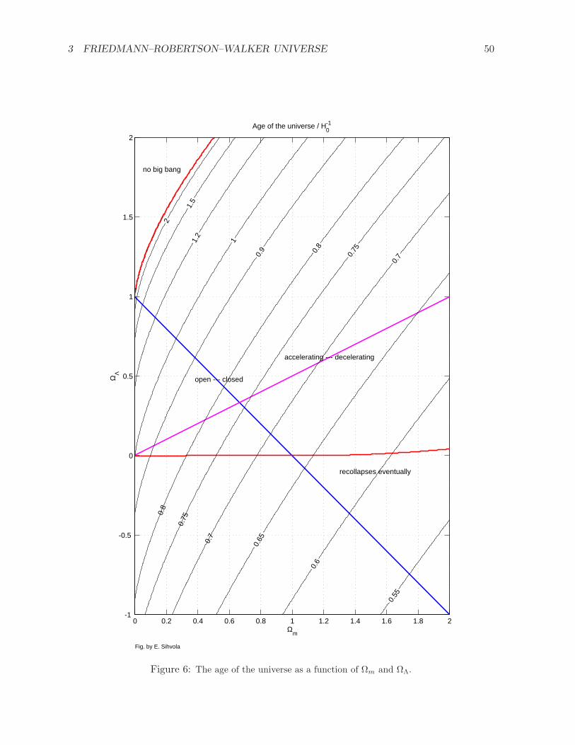
3 FRIEDMANN–ROBERTSON–WALKER UNIVERSE 50

0 0.2 0.4 0.6 0.8 1 1.2 1.4 1.6 1.8 2-1

-0.5

0

0.5

1

1.5

2

open --- closed

accelerating --- decelerating

no big bang

recollapses eventually

Ωm

ΩΛ

Age of the universe / H0-1

0.55

0.6

0.650.7

0.75

0.8

0.70.

750.8

0.9

11.2

1.5

2

Fig. by E. Sihvola

Figure 6: The age of the universe as a function of Ωm and ΩΛ.

3 FRIEDMANN–ROBERTSON–WALKER UNIVERSE 51

0.0 0.5 1.0 1.5 2.0 2.5 3.0 3.5 4.0redshift

0.0

0.2

0.4

0.6

0.8

1.0

1.2

1.4

1.6

1.8

2.0

dist

ance

(H0-1

)

Matter only

0.0 0.5 1.0 1.5 2.0 2.5 3.0 3.5 4.0redshift

0.0

0.2

0.4

0.6

0.8

1.0

1.2

1.4

1.6

1.8

2.0

dist

ance

(H0-1

)

Flat universe

Figure 7: The distance-redshift relation, Eq. (116), for a) the matter-only universe ΩΛ = 0, Ωm = 0,0.2,. . . ,1.8 (from top to bottom) b) the flat universe Ω0 = 1 (ΩΛ = 1− Ωm), Ωm = 0, 0.05, 0.2, 0.4, 0.6,0.8, 1.0, 1.05 (from top to bottom). The thick line in both cases is the Ωm = 1, ΩΛ = 0 model.

This is the distance-redshift relation.

Example: How does the comoving distance depend on cosmological parameters. We canignore Ωr, since it makes such a small contribution. Noting that Ωk = 1 − Ω0 and Ωm = Ω0 − ΩΛ wewrite (116) as

dc(z) = H−10

∫ 1

11+z

da√

Ω0(a− a2)− ΩΛ(a− a4) + a2. (117)

We see that it depends on three independent cosmological parameters, for which we have taken H0,Ω0, and ΩΛ. In this parametrization, the distance at a given redshift is proportional to the Hubbledistance, H−1

0 . If we give the distance in units of H−10 , then it depends only on the two remaining

parameters, Ω0 and ΩΛ. If we increase Ω0 keeping ΩΛ constant (meaning that we increase Ωm), thedistance corresponding to a given redshift decreases. This is because the universe has expanded fasterin the past (see Fig. 5), so that there is less time between a given a = 1/(1 + z) and the present. Thedistance to the galaxy with redshift z is shorter, because photons have had less time to travel. Whereasif we increase ΩΛ with a fixed Ω0 (meaning that we decrease Ωm), we have the opposite situation andthe distance increases. Note that (a− a2) and (a− a4) are always positive since 0 < a ≤ 1.

If a galaxy (with some redshift z) has stayed at the same coordinate value r, i.e., it has nopeculiar velocity, then the comoving distance to it is equal to its present distance. The actualdistance to the galaxy at the time t1 the light left the galaxy is

dp1(z) =dc(z)

1 + z. (118)

We encounter the beginning of time, t = 0, at a = 0 or z = ∞. Thus the comoving distancelight has travelled during the entire age of the universe, the horizon distance, is

dchor = H−10

∫ 1

0

da√

ΩΛa4 +Ωka2 +Ωma+Ωr

. (119)

3 FRIEDMANN–ROBERTSON–WALKER UNIVERSE 52

The simplest cases15, where only one of the terms under the square root is nonzero, give:

radiation dominated (Ωr = Ω0 = 1): dchor = H−10 = 2t0

matter dominated (Ωm = Ω0 = 1): dchor = 2H−10 = 3t0

curvature dominated (Ω0 = 0): dchor = ∞vacuum dominated (ΩΛ = Ω0 = 1): dchor = ∞ .

These results can be applied also at other times, e.g., during the radiation-dominated epochthe horizon distance was related to the Hubble parameter and age by dphor = H−1 = 2t andduring the matter-dominated epoch by dphor = 2H−1 = 3t (assuming that epoch had alreadylasted long enough so that we can ignore the effect of the earlier epochs on the age and horizondistance). Returning to the present time, we know that Ωr is so small that ignoring that termcauses negligible error.

Example: Distance and redshift in the flat matter-dominated universe. Let us look at thesimplest case, (Ωm,ΩΛ) = (1, 0) (with Ωr ≈ 0), in more detail. Now Eq. (116) is just

dc(z) = H−10

∫ 1

11+z

da

a1/2= 2H−1

0

(

1− 1√1 + z

)

. (120)

Expanding 1/√1 + z = 1− 1

2z + 3

8z2 − 5

16z3 · · · we get

dc(z) = H−10 (z − 3

4z2 +

5

8z3 − · · · ) (121)

so that for small redshifts, z ≪ 1 we get the Hubble law, z = H0d0. At the time when the light we seeleft the galaxy, its distance was

dp1(z) =1

1 + zdc(z) = a(t)r = 2H−1

0

(1

1 + z− 1

(1 + z)3/2

)

(122)

= H−10 (z − 7

4z2 +

19

8z3 − · · · ) (123)

so the Hubble law is valid for small z independent of our definition of distance.The distance dp(t) = a(t)r to the galaxy grows with the velocity dp = ra = raH , so that today

dp = rH0 = dcH0 = 2(1− 1/√1 + z). This equals 1 (the speed of light) at z = 3.

We note that dp1(z) has a maximum dp1(z) =827H−1

0 at z = 54

(1 + z = 94). This corresponds to the

comoving distance dc(z) = 23H−1

0 . See Fig. 9. Galaxies that are further out were thus closer when thelight left, since the universe was then so much smaller.

The distance to the horizon in this simplest case is

dchor ≡ dc(z = ∞) = 2H−10 = 3t0. (124)

Example: Effect of radiation. Consider the flat universe (Ωk = 0). Ignoring radiation, withΩm = 0.3, ΩΛ = 0.7, we get for the age of the universe, time since photon decoupling (z = 1090), time

15Of these cases, the strict forms of the two last ones, pure curvature (Ω0 = 0) and pure vacuum (ΩΛ = Ω0 = 1)do not actually fit in the FRW framework, where the starting assumption was spatial homogeneity that formedthe basis of separation between time and space. This separation requires a physical quantity that evolves in time,in practice the energy density ρ(t), so that the t = const slices can be defined as the ρ = const hypersurfaces. Nowin these two cases, ρ = const (either 0 or the vacuum value) also in time, and does not provide this separation.These cases are called the Milne universe and the de Sitter space (or anti-de Sitter space for ρvac < 0) and arediscussed in the General Relativity course. For our purposes, we should instead consider these as limiting caseswhere there is also a density component that is just very small (a nonzero Ωm or Ωr that is ≪ 1). Then thisother component necessarily becomes important in the early universe, as a → 0. This means that dhor is not ∞,just very large. The same applies to the “infinite” age of the vacuum-dominated universe.

3 FRIEDMANN–ROBERTSON–WALKER UNIVERSE 53

0 0.2 0.4 0.6 0.8 1 1.2 1.4 1.6 1.8 2-1

-0.5

0

0.5

1

1.5

2

open --- closed

accelerating --- decelerating

no big bang

recollapses eventually

Ωm

ΩΛ

Horizon / H0-1

1.6

1.7

1.8

1.92

2.4

3

22.2

2.4

2.7

3

3.5

4

5

67

Fig. by E. Sihvola

Figure 8: The horizon as a function of Ωm and ΩΛ.

3 FRIEDMANN–ROBERTSON–WALKER UNIVERSE 54

since z = 10, horizon distance, distance to last scattering sphere, and distance to z = 10 (the most distantgalaxies observed):

t0 = H−10

∫ 1

0

da√Ωma−1 +ΩΛa2

= 0.964099H−10

t0 − tdec = H−10

∫ 1

1/1091

da√Ωma−1 +ΩΛa2

= 0.964066H−10

t0 − t(z = 10) = H−10

∫ 1

1/11

da√Ωma−1 +ΩΛa2

= 0.930747H−10

dchor = H−10

∫ 1

0

da√Ωma+ΩΛa4

= 3.30508H−10

dc(z = 1090) = H−10

∫ 1

1/1091

da√Ωma+ΩΛa4

= 3.19453H−10

dc(z = 10) = H−10

∫ 1

1/11

da√Ωma+ΩΛa4

= 2.20425H−10 . (125)

Include then radiation with Ωr = 0.000085 (we learn in Chapter 4 that this value corresponds to h = 0.7)and subtract it from matter so that Ωm = 0.299915, ΩΛ = 0.7. Now we get

t0 = H−10

∫ 1

0

da√Ωra−2 +Ωma−1 +ΩΛa2

= 0.963799H−10

t0 − tdec = H−10

∫ 1

1/1091

da√Ωra−2 +Ωma−1 +ΩΛa2

= 0.963772H−10

t0 − t(z = 10) = H−10

∫ 1

1/11

da√Ωra−2 +Ωma−1 +ΩΛa2

= 0.930586H−10

dchor = H−10

∫ 1

0

da√Ωr +Ωma+ΩΛa4

= 3.244697H−10

dc(z = 1090) = H−10

∫ 1

1/1091

da√Ωr +Ωma+ΩΛa4

= 3.17967H−10

dc(z = 10) = H−10

∫ 1

1/11

da√Ωr +Ωma+ΩΛa4

= 2.20348H−10 . (126)

(All integrals were done numerically with WolframAlpha, although the first three in (125) could have beendone analytically.) The effect of radiation on these numbers is thus rather small compared to accuracyof observations in cosmology.

Just like any planar map of the surface of Earth must be distorted, so is it for the curvedspacetime. Even in the flat-universe case, the spacetime is curved due to the expansion. Thusany spacetime diagram is a distortion of the true situation. In Figs. 9 and 10 there are threedifferent ways of drawing the same spacetime diagram. In the first one the vertical distance isproportional to the cosmic time t, the horizontal distance to the proper distance at that time,dp(t). The second one is in the comoving coordinates (t, r), so that the horizontal distance isproportional to the comoving distance dc (Note that for Ω = 1, i.e., K = 0, we have dc = r, seeEq. (29)). The third one is in the conformal coordinates (η, r). This one has the advantage thatlight cones are always at a 45 angle. This is thus the “Mercator projection”16 spacetime.

Angular diameter distance: The comoving angular diameter distance is given by thecoordinate r = fK(dc) = dcA so that using the distance-redshift relation, Eq. (116), and dropping

16The Mercator projection is a way of drawing a map of the Earth so that the points of compass correspond tothe same direction everywhere on the map, e.g., northeast and northwest are always 45 from the north direction.

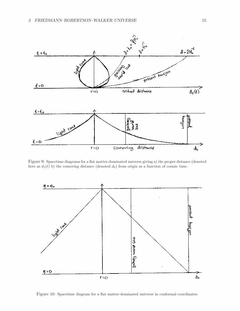
3 FRIEDMANN–ROBERTSON–WALKER UNIVERSE 55

Figure 9: Spacetime diagrams for a flat matter-dominated universe giving a) the proper distance (denotedhere as d1(t) b) the comoving distance (denoted d0) from origin as a function of cosmic time.

Figure 10: Spacetime diagram for a flat matter-dominated universe in conformal coordinates.

3 FRIEDMANN–ROBERTSON–WALKER UNIVERSE 56

0.0 0.5 1.0 1.5 2.0 2.5 3.0 3.5 4.0redshift

0.0

0.2

0.4

0.6

0.8

1.0

1.2

1.4

1.6

1.8

2.0an

gula

rdi

amet

erdi

stan

ce(H

0-1)

Matter only

0.0 0.5 1.0 1.5 2.0 2.5 3.0 3.5 4.0redshift

0.0

0.2

0.4

0.6

0.8

1.0

1.2

1.4

1.6

1.8

2.0

angu

lar

diam

eter

dist

ance

(H0-1

)

Flat universe

Figure 11: The angular diameter distance -redshift relation, Eq. (129), for a) the matter-only universeΩΛ = 0, Ωm = 0, 0.2,. . . ,1.8 (from top to bottom) b) the flat universe Ω0 = 1 (ΩΛ = 1 − Ωm), Ωm = 0,0.05, 0.2, 0.4, 0.6, 0.8, 1.0, 1.05 (from top to bottom). The thick line in both cases is the Ωm = 1, ΩΛ = 0model. Note how the angular diameter distance decreases for large redshifts, meaning that the objectthat is farther away may appear larger on the sky. In the flat case, this is an expansion effect, an objectwith a given size occupies a larger comoving volume in the earlier, smaller universe. In the matter-onlycase, the effect is enhanced by space curvature effects for the closed (Ωm > 1) models.

Ωr, we have

dcA(z) = fK

[1

H0

∫ 1

11+z

da√

Ω0(a− a2)− ΩΛ(a− a4) + a2

]

= H−10

1√Ωkfk

(√

ΩkH0

∫ z

0

dz′

H(z′)

)

, (127)

where we defined (note k instead of K)

fk(x) ≡

sin(x) , (K > 0)

x , (K = 0)

sinh(x) , (K < 0)

(128)

for the comoving angular diameter distance and

dA(z) = dcA(z)/(1 + z) =1

1 + zfK

[1

H0

∫ 1

11+z

da√

Ω0(a− a2)− ΩΛ(a− a4) + a2

]

, (129)

for the angular diameter distance.For a flat universe the comoving angular diameter distance is equal to the comoving distance,

dcA(z) = dc(z) = H−10

∫ 1

1

1+z

da√

Ω0(a− a2)− ΩΛ(a− a4) + a2. (130)

We shall later (in Cosmology II) use the angular diameter distance to relate the observedanisotropies of the cosmic microwave background to the physical length scale of the densityfluctuations they represent. Since this length scale can be calculated from theory, their observedangular size gives us information of the cosmological parameters.

3 FRIEDMANN–ROBERTSON–WALKER UNIVERSE 57

0.0 0.5 1.0 1.5 2.0 2.5 3.0 3.5 4.0redshift

0.0

0.2

0.4

0.6

0.8

1.0

1.2

1.4

1.6

1.8

2.0co

mov

ing

angu

lar

diam

eter

dist

ance

(H0-1

)Matter only

0.0 0.5 1.0 1.5 2.0 2.5 3.0 3.5 4.0redshift

0.0

0.2

0.4

0.6

0.8

1.0

1.2

1.4

1.6

1.8

2.0

com

ovin

gan

gula

rdi

amet

erdi

stan

ce(H

0-1)

Flat universe

Figure 12: Same as Fig. 11, bur for the comoving angular diameter distance. Now the expansion effectis eliminated. For the closed models (for Ωm > 1 in the case of ΩΛ = 0) even the comoving angulardiameter distance may begin to decrease at large enough redshifts. This happens when we are lookingbeyond

√Kχ = π/2, where the universe “begins to close up”. The figure does not go to high enough

z to show this for the parameters used. Note how for the flat universe the comoving angular diameterdistance is equal to the comoving distance (see Fig. 7).

Luminosity distance: From Eq. (46),

dL ≡√

L

4πl= (1 + z)r = (1 + z)dcA(z) = (1 + z)2dA(z)

As we discussed in Chapter 1, astronomers have the habit of giving luminosities as magni-tudes. From the definitions of the absolute and apparent magnitude,

M ≡ −2.5 lgL

L0, m ≡ −2.5 lg

l

l0, (131)

and Eq. (41), we have that the distance modulus m−M is given by the luminosity distance as

m−M = −2.5 lgl

L

L0

l0= 5 lg dL + 2.5 lg 4π

l0L0

= −5 + 5 lg dL(pc) . (132)

(As explained in Chapter 1, the constants L0 and l0 are chosen so as to give the value −5 forthe constant term, when dL is given in parsecs.) For a set of standard candles, all having thesame absolute magnitude M , we find that their apparent magnitudes m should be related totheir redshift z as

m(z) = M − 5 + 5 lg dL(pc)

= M − 5− 5 lgH0 + 5 lg

(1 + z)H0fK

(

H−10

∫ 1

1

1+z

dx√

Ω0(x− x2)− ΩΛ(x− x4) + x2

)

= M − 5− 5 lgH0 + 5 lg

(1 + z)

√−KΩk

× (133)

×fK[√

Ωk

−K

∫ 1

11+z

dx√

Ω0(x− x2)−ΩΛ(x− x4) + x2

]

= M − 5− 5 lgH0 + 5 lg

1 + z√

|Ωk|fk

(√

|Ωk|∫ 1

11+z

dx√

Ω0(x− x2)− ΩΛ(x− x4) + x2

)

.

3 FRIEDMANN–ROBERTSON–WALKER UNIVERSE 58

0.0 0.5 1.0 1.5 2.0 2.5 3.0 3.5 4.0redshift

0

1

2

3

4

5

6

7

8

9

10

lum

inos

itydi

stan

ce(H

0-1)

Matter only

0.0 0.5 1.0 1.5 2.0 2.5 3.0 3.5 4.0redshift

0

1

2

3

4

5

6

7

8

9

10

lum

inos

itydi

stan

ce(H

0-1)

Flat universe

Figure 13: Same as Fig. 11, bur for the luminosity distance. Note how the vertical scale now extendsto 10 Hubble distances instead of just 2, to have room for the much more rapidly increasing luminositydistance.

0.0 0.5 1.0 1.5 2.0 2.5 3.0 3.5 4.0redshift

-5

-4

-3

-2

-1

0

1

2

3

4

5

mag

nitu

de

Matter only

0.0 0.5 1.0 1.5 2.0 2.5 3.0 3.5 4.0redshift

-5

-4

-3

-2

-1

0

1

2

3

4

5

mag

nitu

de

Flat universe

Figure 14: Same as Fig. 11, bur for the magnitude-redshift relation. The constant M − 5 − 5 lgH0 inEq. (134), which is different for different classes of standard candles, has been arbitrarily set to 0.

3 FRIEDMANN–ROBERTSON–WALKER UNIVERSE 59

0.0 0.2 0.4 0.6 0.8 1.0 1.2 1.4 1.6 1.8 2.0redshift

-0.4

-0.2

0.0

0.2

0.4

0.6

0.8

1.0

m

relative difference in m(z)

Figure 15: The difference between the magnitude-redshift relation of the different models in Fig. 14 fromthe reference model Ωm = 1, ΩΛ = 0 (which appears as the horizontal thick line). The red (solid) linesare for the matter-only (ΩΛ = 0) models and the blue (dashed) lines are for the flat (Ω0 = 1) models.

We find that the Hubble constant H0 contributes only to a constant term in this magnitude-

redshift relation. If we just know that all the objects have the same M , but do not know thevalue of M , we cannot use the observed m(z) to determine H0, since both M and H0 contributeto this constant term. On the other hand, the shape of the m(z) curve depends only on the twoparameters Ω0 and ΩΛ (see Fig. 15).

Type Ia supernovae (SNIa) are fairly good standard candles.17 Two groups, the SupernovaCosmology Project18 and the High-Z Supernova Search Team19 have been using observationsof such supernovae up to redshifts z ∼ 2 to try to determine the values of the cosmologicalparameters Ω0 and ΩΛ.

In 1998 they announced [3, 4] that their observations are inconsistent with a matter-dominateduniverse, i.e., with ΩΛ = 0. In fact their observations required that the expansion of the universeis accelerating. This result was named the “Breakthrough of the Year” by the Science maga-zine [5]. Later more accurate observations by these and other groups have confirmed this result.This SNIa data is one of the main arguments for the existence of dark energy in the universe.20

See Fig. 16 for SNIa data from 2004, and Fig. 17 for a determination of Ωm and ΩΛ from thisdata. As you can see, the data is not good enough for a simultaneous accurate determination ofboth Ωm and ΩΛ. But by assuming a flat universe, Ω0 = 1, Riess et al. [6] found ΩΛ = 0.71+0.03

−0.05

(⇒ Ωm = 0.29+0.05−0.03). (The main evidence for a flat universe, Ω0 ≈ 1 comes from the CMB

anisotropy, which we shall discuss later, in Cosmology II)

17To be more precise, they are “standardizable candles”, i.e., their peak absolute magnitudes M vary, but theseare related to their observable properties in a way that can be determined.

18http://supernova.lbl.gov/19http://cfa-www.harvard.edu/cfa/oir/Research/supernova/HighZ.html, http://www.nu.to.infn.it/exp/all/hzsnst/20The other main argument comes from combining CMB anisotropy and large-scale-structure data, and will be

discussed in Cosmology II.

3 FRIEDMANN–ROBERTSON–WALKER UNIVERSE 60

-1.0

-0.5

0.0

0.5

1.0

∆(m

-M)

(mag

)

HST DiscoveredGround Discovered

0.0 0.5 1.0 1.5 2.0z

-0.5

0.0

0.5

∆(m

-M)

(mag

)

ΩM=1.0, ΩΛ=0.0

high-z gray dust (+ΩM=1.0)Evolution ~ z, (+ΩM=1.0)

Empty (Ω=0)ΩM=0.27, ΩΛ=0.73"replenishing" gray Dust

Figure 16: Supernova Ia luminosity-redshift data. The top panel shows all supernova of the data set. Thebottom panel show the averages from different redshift bins. The curves corresponds to three differentFRW cosmologies, and some alternative explanations: “dust” refers to the possibility that the universe isnot transparent, but some photons get absorbed on the way; “evolution” to the possibility that the SNIaare not standard candles, but were different in the younger universe, so that M = M(z). From Riess etal., astro-ph/0402512 [6].

0.0 0.5 1.0 1.5 2.0 2.5ΩM

-1

0

1

2

3

ΩΛ

68.3

%

95.4

%

99.7

%

No Big

Bang

Ωtot =1

Expands to Infinity

Recollapses ΩΛ=0

Open

Closed

Accelerating

Decelerating

q0=0

q0=-0.5

q0=0.5

^

Figure 17: Ωm and ΩΛ determined from the Supernova Ia data. The dotted contours are the old 1998results[3]. From Riess et al., astro-ph/0402512 [6].

3 FRIEDMANN–ROBERTSON–WALKER UNIVERSE 61

We have in the preceding assumed that the mysterious dark energy component of the uni-verse is vacuum energy, or indistinguishable from a cosmological constant, so that pde = −ρde.Making the assumption21 that the equation-of-state parameter wde ≡ pde/ρde for dark energy isa constant, but not necessarily equal to −1, Riess et al. [6] found the limits −1.48 < wde < −0.72,when they assumed a flat universe, and used an independent limit on Ωm from other cosmologicalobservations.

21There is no theoretical justification for this assumption. It is just done for simplicity since the present datais not good enough for determining a larger number of free parameters in the dark-energy equation of state to ameaningful accuracy.

3 FRIEDMANN–ROBERTSON–WALKER UNIVERSE 62

3.3 Concordance Model

Currently the simplest cosmological model that fits all cosmological observations reasonablywell is the ΛCDM model, also called the Concordance Model (since it fits different kinds ofobservations) or the standard model of cosmology (since it is often now assumed in studies thatrelate to cosmology but focus on other questions than the cosmological model). In the name,Λ stands for the cosmological constant, i.e., dark energy is assumed to be vacuum energy andto dominate the energy density of the universe today, and CDM for cold dark matter, which isassumed to make up most of the matter in the universe.

The ΛCDM model includes a number of assumptions related to primordial perturbations, i.e.,deviations from the homogeneous FRW model, that we will discuss in Cosmology II, but for thepresent discussion the relevant part of the ΛCDM model is that the “unperturbed” homogeneous“background” model, a good approximation for large distance scales, is the flat FRW universewith Ω0 = 1 ≈ ΩΛ + Ωm. Often the term “Concordance Model” is used for this FRW model,and the term ΛCDM model is used when also the other assumptions are included. We adoptthis usage.

The expansion law a(t) of the Concordance Model is solved from

da

dt= H0

√

Ωma−1 +ΩΛa2 , (134)

which is easier to integrate from

t(a) = H−10

∫ a

0

da√

Ωma−1 +ΩΛa2= H−1

0

∫ a

0

a1/2da√

Ωm +ΩΛa3

=2

3H−1

0

1√ΩΛ

∫ y

0

dy√

1 + y2=

2

3H−1

0

1√ΩΛ

arsinh

[√

ΩΛ

Ωma3/2

]

, (135)

where we used the substitution y =√

ΩΛ/Ωm a3/2. Inverting this, we have the expansion law

a(t) =

(Ωm

ΩΛ

)1/3

sinh2/3(32

√

ΩΛH0t)

. (136)

At early times, t ≪ (2/3√ΩΛ)H

−10 , the expansion is decelerating and a ∝ t2/3 (the matter-

dominated era):

a(t) ≈(9Ωm

4

)1/3

H2/30 t2/3 . (137)

At late times, t ≫ (2/3√ΩΛ)H

−10 , the expansion is exponential and accelerating (the vacuum-

dominated era):

a(t) ≈(

Ωm

4ΩΛ

)1/3

e√ΩΛH0t . (138)

From above, the age-redshift relation is

t(z) =2

3H−1

0

1√ΩΛ

arsinh

[√

ΩΛ

Ωm(1 + z)−3/2

]

, (139)

and the present age of the universe is

t0 =2

3H−1

0

1√ΩΛ

arsinh

√

ΩΛ

Ωm(140)

3 FRIEDMANN–ROBERTSON–WALKER UNIVERSE 63

In the concordance model, there are two energy-density components, ρvac = const and ρm ∝a−3, so that ρ = ρvac + ρm and p = −ρvac. From the second Friedmann equation

a

a= −4πG

3(ρ+ 3p) = −4πG

3(ρm − 2ρvac) (141)

we see that the deceleration turns into accelaration when ρvac =12ρm. Since

ρvacρm

=ΩΛ

Ωm

(a

a0

)3

= sinh2(32

√

ΩΛH0t)

, (142)

we get that this happens when

a =1

1 + z=

(Ωm

2ΩΛ

)1/3

and tacc =2

3H−1

0

1√ΩΛ

arsinh1√2. (143)

The vacuum and matter energy densities become equal later, when

a =1

1 + z=

(Ωm

ΩΛ

)1/3

and teq =2

3H−1

0

1√ΩΛ

arsinh(1) . (144)

Here

arsinh1√2= 0.65848 and arsinh(1) = 0.88137 . (145)

For ΩΛ = 0.7 and Ωm = 0.3,

arsinh

√

ΩΛ

Ωm= arsinh(1.5275) = 1.2099 (146)

andtacc = 0.5247H−1

0 teq = 0.7023H−10 t0 = 0.9641H−1

0 . (147)

In the concordance model the distance-redshift relation appears not to have a closed form interms of elementary functions, so we need to integrate it numerically. The (comoving) distanceto the horizon is

dchor = H−10

∫ 1

0

da√

ΩΛa4 +Ωma. (148)

which for ΩΛ = 0.7 and Ωm = 0.3 gives dchor = 3.305H−10 .

These results are modified somewhat by inclusion of the effect of radiation (Ωr ≈ 10−4),which requires integrating also t(a) numerically.

Planck 2018 best-fit concordance model. The best-fit ΛCDM model to the final release ofPlanck satellite data (we discuss this in Cosmology II; see p. 14, Table I, Plik best-fit in [9]) has

Ωm = 0.3158 Ωr = 9.232× 10−5 H0 = 67.32 km/s/Mpc (149)

(and ΩΛ = 1− Ωm − Ωr).22 The Hubble distance and time are then

H−10 = 4453.2Mpc = 14.525× 109 yr . (150)

22We cheat here a little bit, by using the value of Ωr corresponding to three massless neutrino species; whereasthe Planck best-fit model assumed one massive neutrino species with mν = 0.06 eV, so that this neutrino speciescounts today as matter (and is included in the Ωm = 0.3158, where it contributes about 0.0014). A truly accuratetreatment would include the change of this species from radiation into matter as the universe expands. It is moreaccurate to include it also in Ωr at all times than not to include it there at all, since Ωr is much more importantat early times.

3 FRIEDMANN–ROBERTSON–WALKER UNIVERSE 64

Including the effect of Ωr, we need to integrate also the age-redshift relation numerically. The age of theuniverse is

t0 = 0.9499H−10 = 13.797Gyr . (151)

For the redshift when acceleration began, one now has to solve a fourth-order equation (done convenientlywith WolframAlpha), to get

aacc =1

1 + zacc= 0.6136 and tacc = 0.5306H−1

0 = 7.707Gyr , (152)

i.e., the expansion began to accelarate 6.09 billion years ago. Matter density was equal to vacuum-energydensity at

aeq =1

1 + zeq= 0.7729 and teq = 0.7100H−1

0 = 10.313Gyr , (153)

i.e., 3.48 billion years ago. The (comoving) horizon distance (to z = ∞) is

dhor = 3.1767H−10 = 14.146Mpc = 46.14× 109 light years . (154)

The comoving distance to the last scattering sphere (z = 1090) is

dls = 3.1138H−10 = 13.867Mpc = 45.23× 109 light years . (155)

We provide a table of different quantities (age and comoving distance) as a function ofredshift for the Planck 2013 (the first data release) best-fit model in Table 1. Table 2 is forour reference model h = 0.7, ΩΛ = 0.7 and Table 3 for the Planck 2018 best-fit model [9]. Thereason for giving them with so many digits in the table is that one can then take differencesbetween the values for different redshifts.

The distant future in the concordance model has interesting properties because of the accel-erating expansion:

1. Distant galaxies will recede from us faster and faster, with the result that it is not possibleto travel from here to the most distant galaxies (“Unreachable” in Fig. 18) we can observenow, even if it there were means to travel with speeds arbitrarily close to the speed oflight. Also light rays from here will never reach those galaxies, and similarly, light rayssent from those galaxies today will never reach us.

2. The (comoving) horizon distance dchor will approach asymptotically a maximum value (the“Future comoving visibility limit” in Fig. 18). Galaxies beyond that will never becomeobservable from here. We already see a sizable fraction of that part of the universe thatwill ever become observable from here. Instead, because the redshifts of distant galaxieswill keep increasing with time, eventually they will disappear from sight because they willbecome so faint (they will still stay within the horizon, since their dc stays constant, anddchor does not decrease with time). The relevant time scale here is of course cosmological;we are referring to a future tens of billions of years from today.

Example: Future comoving visibility limit. The comoving distance traveled by a light ray sincet = 0 until t = ∞ is

dc =

∫

dχ =

∫∞

0

dt

a(t)=

(ΩΛ

Ωm

)1/32

3√ΩΛH0

∫∞

0

sinh−2/3 x dx

= Ω−1/6Λ Ω−1/3

m

Γ(16)Γ(1

3)

3√π

H−10 = 2.8044Ω

−1/6Λ Ω−1/3

m H−10 . (156)

With Ωm = 0.3 this gives dc = 4.4457H−10 . The integral was done by converting it to the Euler B

function

B(p, q) ≡∫ 1

0

tp−1(1 − t)q−1 dt =Γ(p)Γ(q)

Γ(p+ q)(157)

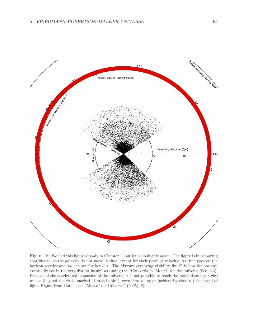
3 FRIEDMANN–ROBERTSON–WALKER UNIVERSE 65

Figure 18: We had this figure already in Chapter 1, but let us look at it again. The figure is in comovingcoordinates, so the galaxies do not move in time, except for their peculiar velocity. As time goes on thehorizon recedes and we can see further out. The “Future comoving visibility limit” is how far one caneventually see in the very distant future, assuming the “Concordance Model” for the universe (Sec. 3.3).Because of the accelerated expansion of the universe it is not possible to reach the most distant galaxieswe see (beyond the circle marked “Unreachable”), even if traveling at (arbitrarily close to) the speed oflight. Figure from Gott et al: “Map of the Universe” (2005) [8].

REFERENCES 66

by the substitution t = tanh2 x, which gives

∫∞

0

sinhµ x dx = 12

∫ 1

0

tµ/2−1/2(1− t)−µ/2−1 = 12B(µ2+ 1

2,−µ

2

)=

Γ(µ2+ 1

2)Γ(−µ

2)

2Γ(12)

(158)

where Γ(12) =

√π.

References

[1] A. Friedmann, Uber die Krummung des Raumes, Zeitschrift fur Physik, 10, 377 (1924).

[2] A. Friedmann, Uber die Moglichkeit einer Welt mit konstanter negativer Krummung des

Raumes, Zeitschrift fur Physik, 21, 326 (1924).

[3] A.G. Riess et al., Astron. J. 116, 1009 (1998)

[4] S. Perlmutter et al., Astrophys. J. 517, 565 (1999)

[5] J. Glantz, Science 282, 2156 (18 Dec 1998)

[6] A.G. Riess et al., Astrophys. J. 607, 665 (2004), astro-ph/0402512

[7] Planck Collaboration, A&A 571, A16 (2014), arXiv:1303.5076v2

[8] J. Richard Gott III et al., A Map of the Universe, Astrophys. J. 624, 463 (2005), astro-ph/0310571.

[9] Planck Collaboration, arXiv:1807.06209v1

REFERENCES 67

Age and distance in the Planck 2013 best-fit concordance model

z t (Gyr) t0 − t (H−10 ) dc (H−1

0 ) dc (Mpc) dc (Gyr)

0 13.83 0 0 0 00.1 12.47 0.0930 0.0976 436 1.4210.2 11.30 0.1737 0.1902 849 2.7700.3 10.27 0.2439 0.2779 1241 4.0460.4 9.38 0.3051 0.3605 1610 5.2500.5 8.60 0.3589 0.4384 1957 6.3840.6 7.91 0.4062 0.5117 2284 7.4500.7 7.30 0.4480 0.5806 2592 8.4540.8 6.76 0.4850 0.6454 2881 9.3970.9 6.28 0.5180 0.7064 3154 10.2851 5.85 0.5475 0.7638 3409 11.1211.5 4.27 0.6562 1.0061 4492 14.6502 3.27 0.7243 1.1922 5322 17.3592.5 2.61 0.7699 1.3397 5981 19.5073 2.14 0.8020 1.4597 6517 21.2554 1.54 0.8436 1.6449 7343 23.9515 1.17 0.8687 1.7823 7957 25.9526 0.928 0.8853 1.8894 8435 27.5117 0.760 0.8969 1.9758 8821 28.7698 0.636 0.9053 2.0474 9141 29.8119 0.543 0.9117 2.1080 9411 30.69410 0.471 0.9167 2.1602 9644 31.45420 0.178 0.9368 2.4553 10962 35.752100 0.0164 0.9479 2.8741 12831 41.8501000 0.000430 0.948955 3.1051 13863 45.2131089 0.000375 0.948959 3.1090 13880 45.271

Table 1: The cosmological parameters assumed here are ΩΛ = 0.6830, Ωm = 0.3169, Ωr = 9.323× 10−5,H0 = 67.15 km/s/Mpc. Credit: Elina Palmgren.

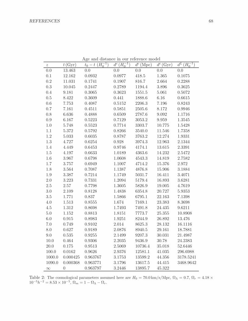
REFERENCES 68

Age and distance in our reference model

z t (Gyr) t0 − t (H−10 ) dc (H−1

0 ) dc (Mpc) dc (Gyr) dL (H−10 )

0.0 13.463 0.0 0.0 0.0 0.0 0.00.1 12.162 0.0932 0.0977 418.5 1.365 0.10750.2 11.031 0.1741 0.1907 816.7 2.664 0.22880.3 10.045 0.2447 0.2789 1194.4 3.896 0.36250.4 9.181 0.3065 0.3623 1551.5 5.061 0.50720.5 8.422 0.3609 0.441 1888.6 6.16 0.66150.6 7.753 0.4087 0.5152 2206.3 7.196 0.82430.7 7.161 0.4511 0.5851 2505.6 8.172 0.99460.8 6.636 0.4888 0.6509 2787.6 9.092 1.17160.9 6.167 0.5223 0.7129 3053.2 9.959 1.35451.0 5.748 0.5523 0.7714 3303.7 10.775 1.54281.1 5.372 0.5792 0.8266 3540.0 11.546 1.73581.2 5.033 0.6035 0.8787 3763.2 12.274 1.93311.3 4.727 0.6254 0.928 3974.3 12.963 2.13441.4 4.449 0.6453 0.9746 4174.1 13.615 2.33911.5 4.197 0.6633 1.0189 4363.6 14.232 2.54721.6 3.967 0.6798 1.0608 4543.3 14.819 2.75821.7 3.757 0.6949 1.1007 4714.2 15.376 2.9721.8 3.564 0.7087 1.1387 4876.8 15.906 3.18841.9 3.387 0.7214 1.1749 5031.7 16.411 3.40712.0 3.223 0.7331 1.2094 5179.4 16.893 3.62812.5 2.57 0.7798 1.3605 5826.9 19.005 4.76193.0 2.109 0.8128 1.4838 6354.8 20.727 5.93533.5 1.771 0.837 1.5866 6795.1 22.163 7.13984.0 1.513 0.8555 1.674 7169.1 23.383 8.36984.5 1.312 0.8698 1.7493 7491.8 24.435 9.62115.0 1.152 0.8813 1.8151 7773.7 25.355 10.89086.0 0.915 0.8983 1.9251 8244.9 26.892 13.4767.0 0.749 0.9102 2.014 8625.3 28.132 16.11168.0 0.627 0.9189 2.0876 8940.5 29.161 18.78819.0 0.535 0.9255 2.1499 9207.3 30.031 21.498710.0 0.464 0.9306 2.2035 9436.9 30.78 24.238320.0 0.175 0.9513 2.5069 10736.4 35.018 52.6446100.0 0.0162 0.9626 2.9376 12581.1 41.035 296.69881000.0 0.000425 0.963767 3.1753 13599.2 44.356 3178.52411090.0 0.000368 0.963771 3.1796 13617.5 44.415 3468.9642∞ 0 0.963797 3.2446 13895.7 45.322

Table 2: The cosmological parameters assumed here are H0 = 70.0 km/s/Mpc, ΩΛ = 0.7, Ωr = 4.18 ×10−5h−2 = 8.53× 10−5, Ωm = 1− ΩΛ − Ωr.

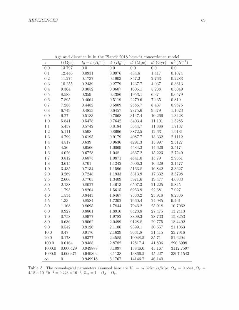
REFERENCES 69

Age and distance in in the Planck 2018 best-fit concordance model

z t (Gyr) t0 − t (H−10 ) dc (H−1

0 ) dc (Mpc) dc (Gyr) dL (H−10 )

0.0 13.797 0.0 0.0 0.0 0.0 0.00.1 12.446 0.0931 0.0976 434.6 1.417 0.10740.2 11.274 0.1737 0.1903 847.2 2.763 0.22830.3 10.255 0.2439 0.2779 1237.7 4.037 0.36130.4 9.364 0.3052 0.3607 1606.1 5.238 0.50490.5 8.583 0.359 0.4386 1953.1 6.37 0.65790.6 7.895 0.4064 0.5119 2279.6 7.435 0.8190.7 7.288 0.4482 0.5809 2586.7 8.437 0.98750.8 6.749 0.4853 0.6457 2875.6 9.379 1.16230.9 6.27 0.5183 0.7068 3147.4 10.266 1.34281.0 5.841 0.5478 0.7642 3403.4 11.101 1.52851.1 5.457 0.5742 0.8184 3644.7 11.888 1.71871.2 5.111 0.598 0.8696 3872.5 12.631 1.91311.3 4.799 0.6195 0.9179 4087.7 13.332 2.11121.4 4.517 0.639 0.9636 4291.3 13.997 2.31271.5 4.26 0.6566 1.0069 4484.2 14.626 2.51741.6 4.026 0.6728 1.048 4667.2 15.223 2.72491.7 3.812 0.6875 1.0871 4841.0 15.79 2.93511.8 3.615 0.701 1.1242 5006.3 16.329 3.14771.9 3.435 0.7134 1.1596 5163.8 16.842 3.36272.0 3.269 0.7248 1.1933 5313.9 17.332 3.57982.5 2.606 0.7705 1.3409 5971.6 19.477 4.69333.0 2.138 0.8027 1.4613 6507.3 21.225 5.8453.5 1.795 0.8264 1.5615 6953.9 22.681 7.0274.0 1.534 0.8443 1.6467 7333.2 23.918 8.23364.5 1.33 0.8584 1.7202 7660.4 24.985 9.4615.0 1.168 0.8695 1.7844 7946.2 25.918 10.70626.0 0.927 0.8861 1.8916 8423.8 27.475 13.24137.0 0.758 0.8977 1.9782 8809.3 28.733 15.82538.0 0.636 0.9062 2.0499 9128.8 29.775 18.44929.0 0.542 0.9126 2.1106 9399.1 30.657 21.106310.0 0.47 0.9176 2.1629 9631.8 31.415 23.791620.0 0.178 0.9377 2.4585 10948.5 35.71 51.6294100.0 0.0164 0.9488 2.8782 12817.4 41.806 290.69981000.0 0.000429 0.949888 3.1097 13848.0 45.167 3112.75971090.0 0.000371 0.949892 3.1138 13866.5 45.227 3397.1543∞ 0 0.949918 3.1767 14146.7 46.140

Table 3: The cosmological parameters assumed here are H0 = 67.32 km/s/Mpc, ΩΛ = 0.6841, Ωr =4.18× 10−5h−2 = 9.223× 10−5, Ωm = 1− ΩΛ − Ωr.

4 Thermal history of the Early Universe

4.1 Relativistic thermodynamics

As we look out in space we can see the history of the universe unfolding in front of our telescopes.However, at redshift z = 1090 our line of sight hits the last scattering surface, from which the cos-mic microwave background (CMB) radiation originates. This corresponds to t = 370 000 years.Before that the universe was not transparent, so we cannot see further back in time, into theearly universe. As explained in Sec. 3, we can ignore curvature and vacuum/dark energy in theearly universe and concern ourselves only with radiation and matter. The isotropy of the CMBshows that matter was distributed homogeneously in the early universe, and the spectrum of theCMB shows that this matter, the “primordial soup” of particles, was in thermodynamic equilib-rium. Therefore we can use thermodynamics to calculate the history of the early universe. Aswe shall see, this calculation leads to predictions (especially the BBN, big bang nucleosynthesis)testable by observation. We shall now discuss the thermodynamics of the primordial soup.

From elementary quantum mechanics we are familiar with the “particle in a box”. Let usconsider a cubic box, whose edge is L (volume V = L3), with periodic boundary conditions.Solving the Schrodinger equation gives us the energy and momentum eigenstates, where thepossible momentum values are

~p =h

L(n1x+ n2y + n3z) (ni = 0,±1,±2, . . .) , (1)

where h is the Planck constant. (The wave function will have an integer number of wavelengthsin each of the three directions.) The state density in momentum space (number of states /∆px∆py∆pz) is thus

L3

h3=

V

h3, (2)

and the state density in the 6-dimensional phase space (~x, ~p) is 1/h3. If the particle has ginternal degrees of freedom (e.g., spin),

density of states =g

h3=

g

(2π)3

(

~ ≡ h

2π≡ 1

)

. (3)

This result is true even for relativistic momenta. The state density in phase space is independentof the volume V , so we can apply it for arbitrarily large systems (e.g., the universe).

For much of the early universe, we can ignore the interaction energies between the particles.Then the particle energy is (according to special relativity)

E(~p) =√

p2 +m2 , (4)

where p ≡ |~p| (momentum, not pressure!), and the states available for the particles are the freeparticle states discussed above.

Particles fall into two classes, fermions and bosons. Fermions obey the Pauli exclusionprinciple: no two fermions can be in the same state.

In thermodynamic equilibrium the distribution function, or the expectation value f of theoccupation number of a state, depends only on the energy of the state. According to statisticalphysics, it is

f(~p) =1

e(E−µ)/T ± 1(5)

where + is for fermions and − is for bosons. (For fermions, where f ≤ 1, f gives the probabilitythat a state is occupied.) This equilibrium distribution has two parameters, the temperature T ,

70

4 THERMAL HISTORY OF THE EARLY UNIVERSE 71

and the chemical potential µ. The temperature is related to the energy density in the systemand the chemical potential is related to the number density n of particles in the system. Notethat, since we are using the relativistic formula for the particle energy E, which includes themass m, it is also “included” in the chemical potential µ. Thus in the nonrelativistic limit, bothE and µ differ from the corresponding quantities of nonrelativistic statistical physics by m, sothat E − µ and the distribution functions remain the same.

If there is no conserved particle number in the system (e.g., a photon gas), then µ = 0 inequilibrium.

The particle density in phase space is the density of states times their occupation number,

g

(2π)3f(~p). (6)

We get the particle density in (ordinary 3D) space by integrating over the momentum space.Thus we find the following quantities:

number density n =g

(2π)3

∫

f(~p)d3p (7)

energy density ρ =g

(2π)3

∫

E(~p)f(~p)d3p (8)

pressure p =g

(2π)3

∫ |~p|23E

f(~p)d3p . (9)

Different particle species i have different masses mi; so the preceding is applied separately toeach particle species. If particle species i has the above distribution for some µi and Ti, we saythe species is in kinetic equilibrium. If the system is in thermal equilibrium, all species have thesame temperature, Ti = T . If the system is in chemical equilibrium (“chemistry” here refers toreactions where particles change into other species), the chemical potentials of different particlespecies are related according to the reaction formulas. For example, if we have a reaction

i+ j ↔ k + l , (10)

thenµi + µj = µk + µl . (11)

Thus all chemical potentials can be expressed in terms of the chemical potentials of conservedquantities, e.g., the baryon number chemical potential, µB. There are thus as many independentchemical potentials, as there are independent conserved particle numbers. For example, if thechemical potential of particle species i is µi, then the chemical potential of the correspondingantiparticle is −µi. We can also have a situation that some reactions are in chemical equilibriumbut others are not.

Thermodynamic equilibrium refers to having all these equilibria, but I will also use the termmore loosely to refer to some subset of them.

As the universe expands, T and µ change, so that energy continuity and particle numberconservation are satisfied. In principle, an expanding universe is not in equilibrium. The expan-sion is however sufficiently slow compared to particle interaction rates, so that the particle soupusually has time to settle close to local equilibrium. (And since the universe is homogeneous, thelocal values of thermodynamic quantities are also global values). Although the expansion wasfaster in the early universe than later, the interaction rates were much higher because of higherdensity and higher particle energies, so that we can have equilibrium in the early universe, butnot later.

From the remaining numbers of fermions (electrons and nucleons) in the present universe,we can conclude that in the early universe we had |µ| ≪ T when T ≫ m. (We don’t know the

4 THERMAL HISTORY OF THE EARLY UNIVERSE 72

chemical potential of neutrinos, but it is usually assumed to be small too). If the temperature ismuch greater than the mass of a particle, T ≫ m, the ultrarelativistic limit, we can approximateE =

√

p2 +m2 ≈ p.For |µ| ≪ T and m ≪ T , we approximate µ = 0 and m = 0 to get the following formulae

n =g

(2π)3

∫

∞

0

4πp2dp

ep/T ± 1=

3

4π2ζ(3)gT 3 fermions

1

π2ζ(3)gT 3 bosons

(12)

ρ =g

(2π)3

∫

∞

0

4πp3dp

ep/T ± 1=

7

8

π2

30gT 4 fermions

π2

30gT 4 bosons

(13)

p =g

(2π)3

∫

∞

0

43πp

3dp

ep/T ± 1=

1

3ρ ≈

1.0505nT fermions

0.9004nT bosons .(14)

For the average particle energy we get

〈E〉 = ρ

n=

7π4

180ζ(3)T ≈ 3.15137T fermions

π4

30ζ(3)T ≈ 2.70118T bosons .

(15)

In the above, ζ is the Riemann zeta function, and ζ(3) ≡ ∑

∞

n=1(1/n3) = 1.202057.

If the chemical potential µ = 0, there are equal numbers of particles and antiparticles. Ifµ 6= 0, we find for fermions in the ultrarelativistic limit T ≫ m (i.e., for m = 0, but µ 6= 0) the“net particle number”

n− n =g

(2π)3

∫

∞

0dp 4πp2

(

1

e(p−µ)/T + 1− 1

e(p+µ)/T + 1

)

=gT 3

6π2

(

π2(µ

T

)

+(µ

T

)3)

(16)

and the total energy density

ρ+ ρ =g

(2π)3

∫

∞

0dp 4πp3

(

1

e(p−µ)/T + 1+

1

e(p+µ)/T + 1

)

=7

8gπ2

15T 4

(

1 +30

7π2

(µ

T

)2+

15

7π4

(µ

T

)4)

. (17)

Note that the last forms in Eqs. (16) and (17) are exact, not just truncated series. (The differencen − n and the sum ρ + ρ lead to a nice cancellation between the two integrals. We don’t getsuch an elementary form for the individual n, n, ρ, ρ, or the sum n+ n and the difference ρ− ρwhen µ 6= 0.)

In the nonrelativistic limit, T ≪ m and T ≪ m − µ, the typical kinetic energies are muchbelow the mass m, so that we can approximate E = m + p2/2m. The second condition, T ≪m − µ, leads to occupation numbers ≪ 1, a dilute system. This second condition is usuallysatisfied in cosmology when the first one is. (It is violated in systems of high density, like whitedwarf stars and neutrons stars.) We can then approximate

e(E−µ)/T ± 1 ≈ e(E−µ)/T , (18)

4 THERMAL HISTORY OF THE EARLY UNIVERSE 73

so that the boson and fermion expressions become equal,1 and we get (exercise)

n = g

(

mT

2π

)3/2

e−m−µT (19)

ρ = n

(

m+3T

2

)

(20)

p = nT ≪ ρ (21)

〈E〉 = m+3T

2(22)

n− n = 2g

(

mT

2π

)3

2

e−m

T sinhµ

T. (23)

In the general case, where neither T ≪ m, nor T ≫ m, the integrals don’t give elementaryfunctions, but n(T ), ρ(T ), etc. need to be calculated numerically for the region T ∼ m.2

By comparing the ultrarelativistic (T ≫ m) and nonrelativistic (T ≪ m) limits we see thatthe number density, energy density, and pressure of a particle species falls exponentially asthe temperature falls below the mass of the particle. What happens is that the particles andantiparticles annihilate each other. (Other reactions may also be involved, and if these particlesare unstable, also their decay contributes to their disappearance.) At higher temperaturesthese annihilation reactions are also constantly taking place, but they are balanced by particle-antiparticle pair production. At lower temperatures the thermal particle energies are no moresufficient for pair production. This particle-antiparticle annihilation takes place mainly (about80%) during the temperature interval T = m → 1

6m. See Fig. 1. It is thus not an instantaneousevent, but takes several Hubble times.

Figure 1: The fall of energy density of a particle species, with mass m, as a function of temperature(decreasing to the right).

4.2 Primordial soup

We shall now apply the thermodynamics discussed in the previous section to the evolution ofthe early universe.

The primordial soup initially consists of all the different species of elementary particles.Their masses range from the heaviest known elementary particle, the top quark (m = 173 GeV)down to the lightest particles, the electron (m = 511 keV), the neutrinos (m = ?) and the

1This approximation leads to what is called Maxwell–Boltzmann statistics; whereas the previous exact formulaegive Fermi–Dirac (for fermions) and Bose–Einstein (for bosons) statistics.

2If we use Maxwell–Boltzmann statistics, i.e., we drop the term ±1, the integrals give modified Bessel functions,e.g., K2(m/T ), and the error is often less than 10%.

4 THERMAL HISTORY OF THE EARLY UNIVERSE 74

photon (m = 0). In addition to the particles of the standard model of particle physics (given inTable 1), there must be other, so far undiscovered, species of particles, at least those that makeup the CDM. As the temperature falls, the various particle species become nonrelativistic and

annihilate at different times.Another central theme is decoupling : as the number densities and particle energies fall with

the expansion, some reaction rates become too low to keep up with the changing equilibrium andtherefore some quantities are “frozen” at their pre-decoupling values. We will encounter neutrinoand photon decoupling later in this chapter; decoupling is also important in BBN (Chapter 5)and for dark matter (Chapter 6).

Table 1: The particles in the standard model of particle physics

Particle Data Group, 2018

Quarks t 173.0 ± 0.4GeV t spin=12 g = 2 · 3 = 6

b 4.15–4.22GeV b 3 colorsc 1.27 ± 0.03GeV cs 92–104MeV sd 4.4–5.2MeV du 1.8–2.7MeV u

72

Gluons 8 massless bosons spin=1 g = 2 16

Leptons τ− 1776.86 ± 0.12MeV τ+ spin=12 g = 2

µ− 105.658MeV µ+

e− 510.999 keV e+

12ντ < 2 eV ντ spin=1

2 g = 1νµ < 2 eV νµνe < 2 eV νe

6

Electroweak W+ 80.379 ± 0.012GeV W− spin=1 g = 3gauge bosons Z0 91.1876±0.0021GeV

γ 0 (< 1× 10−18 eV) g = 211

Higgs boson (SM) H0 125.18 ± 0.16GeV spin=0 g = 1 1

gf = 72 + 12 + 6 = 90gb = 16 + 11 + 1 = 28

The mass limits for neutrinos come from a direct laboratory upper limit for νe and evidence from neutrinooscillations that the differences in neutrino masses are much smaller. We can use cosmology to put tighterlimits to neutrino masses. Neutrinos are special in that the antineutrino is just the other spin state ofthe neutrino. Therefore we put g = 1 for their internal degrees of freedom when we count antineutrinosseparately.

4 THERMAL HISTORY OF THE EARLY UNIVERSE 75

According to the Friedmann equation the expansion of the universe is governed by the totalenergy density

ρ(T ) =∑

ρi(T ) ,

where i runs over the different particle species. Since the energy density of relativistic speciesis much greater than that of nonrelativistic species, it suffices to include the relativistic speciesonly. (This is true in the early universe, during the radiation-dominated era, but not at latertimes. Eventually the rest masses of the particles left over from annihilation begin to dominateand we enter the matter-dominated era.) Thus we have

ρ(T ) =π2

30g∗(T )T

4, (24)

where

g∗(T ) = gb(T ) +7

8gf (T ),

and gb =∑

i gi over relativistic bosons and gf =∑

i gi over relativistic fermions. These resultsassume thermal equilibrium. For pressure we have p(T ) ≈ 1

3ρ(T ).The above is a simplification of the true situation: Since the annihilation takes a long time,

often the annihilation of some particle species is going on, and the contribution of this speciesdisappears gradually. Using the exact formula for ρ we define the effective number of degrees of

freedom g∗(T ) by

g∗(T ) ≡30

π2

ρ

T 4. (25)

We can also define

g∗p(T ) ≡90

π2

p

T 4≈ g∗(T ) . (26)

These can then be calculated numerically (see Figure 1).We see that when there are no annihilations taking place, g∗p = g∗ = const ⇒ p = 1

3ρ ⇒ρ ∝ a−4 and ρ ∝ T 4, so that T ∝ a−1. Later in this chapter we shall calculate the T (a) relationmore exactly (including the effects of annihilations).

For T > mt = 173 GeV, all known particles are relativistic. Adding up their internal degreesof freedom we get

gb = 28 gluons 8×2, photons 2, W± and Z0 3×3, and Higgs 1

gf = 90 quarks 12×6, charged leptons 6×2, neutrinos 3×2

g∗ = 106.75.

The electroweak (EW) transition3 took place close to this time (Tc ∼ 100 GeV). It appearsthat g∗ was the same before and after this transition. Going to earlier times and higher temper-atures, we expect g∗ to get larger than 106.75 as new physics (new unknown particle species)comes to play.4

3This is usually called the electroweak phase transition, but the exact nature of the transition is not known.Technically it may be a cross-over rather than a phase transition, meaning that it occurs over a temperaturerange rather than at a certain critical temperature Tc.

4A popular form of such new physics is supersymmetry, which provides supersymmetric partners, whose spindiffer by 1

2, for the known particle species, so that fermions have supersymmetric boson partners and bosons have

supersymmetric fermion partners. Since these partners have not been so far observed, supersymmetry must bebroken, allowing these partners to have much higher masses. In the minimal supersymmetric standard model(MSSM) the new internal degrees of freedom are as follows: Spin-0 bosons (scalars): sleptons 9 · 2 = 18, squarks6 · 2 · 2 · 3 = 72 (although there is only one spin degree instead of 2, there is another degree of freedom, so thatwe get the same 18+72 as for leptons and quarks), and a new complex Higgs doublet 2 · 2 = 4. Spin- 1

2fermions:

neutralinos 4 · 2 = 8, charginos 2 · 2 · 2 (two charge degrees and two spin degrees), and gluinos 8 · 2 = 16. Thisgives g∗ = 106.75 + 94 + 7

8· 32 = 228.75. Other supersymmetric models have somewhat more degrees of freedom

but some of the new degrees of freedom may be very heavy (1010 . . . 1016 GeV).[1]

4 THERMAL HISTORY OF THE EARLY UNIVERSE 76

-6 -5 -4 -3 -2 -1 0 1 2-lg(T/MeV)

100

2

5

101

2

5

102

2

g *

Figure 2: The functions g∗(T ) (solid), g∗p(T ) (dashed), and g∗s(T ) (dotted) calculated for thestandard model particle content.

Let us now follow the history of the universe starting at the time when the EW transitionhas already happened. We have T ∼ 100 GeV, t ∼ 20 ps, and the t quark annihilation is on theway. The Higgs boson and the gauge bosons W±, Z0 annihilate next. At T ∼ 10 GeV, we haveg∗ = 86.25. Next the b and c quarks annihilate and then the τ meson, so that g∗ = 61.75.

4.3 QCD transition

Before s quark annihilation would take place, something else happens: the QCD transition

(also called the quark–hadron transition). This takes place at T ∼ 150 MeV, t ∼ 20 µs. Thetemperature and thus the quark energies have fallen so that the quarks lose their so-calledasymptotic freedom, which they have at high energies. The interactions between quarks andgluons (the strong nuclear force, or the color force) become important (so that the formulae forthe energy density in Sec. 4.1 no longer apply) and soon a phase transition takes place. Thereare no more free quarks and gluons; the quark-gluon plasma has become a hadron gas. Thequarks and gluons have formed bound three-quark systems, called baryons, and quark-antiquarkpairs, called mesons. The lightest baryons are the nucleons: the proton and the neutron. Thelightest mesons are the pions: π±, π0. Baryons are fermions, mesons are bosons.

There are very many different species of baryons and mesons, but all except pions are non-relativistic below the QCD transition temperature. Thus the only particle species left in largenumbers are the pions, muons, electrons, neutrinos, and the photons. For pions, g = 3, so nowg∗ = 17.25.

4 THERMAL HISTORY OF THE EARLY UNIVERSE 77

Table 2: History of g∗(T )

T ∼ 200 GeV all present 106.75

T ∼ 100 GeV EW transition (no effect)

T < 170 GeV top annihilation 96.25

T < 80 GeV W±, Z0, H0 86.25

T < 4 GeV bottom 75.75

T < 1 GeV charm, τ− 61.75

T ∼ 150 MeV QCD transition 17.25 (u,d,s,g→ π±,0, 47.5 → 3)

T < 100 MeV π±, π0, µ− 10.75 e±, ν, ν, γ left

T < 500 keV e− annihilation (7.25) 2 + 5.25(4/11)4/3 = 3.36

This table gives what value g∗(T ) would have after the annihilation of a particle species is over assumingthe annihilation of the next species had not begun yet. In reality they overlap in many cases. Thetemperature value at the left is the approximate mass of the particle in question and indicates roughlywhen annihilation begins. The temperature is much smaller when the annihilation is over. Therefore topannihilation is placed after the EW transition. The top quark receives its mass in the EW transition, soannihilation only begins after the transition.

4.4 Neutrino decoupling and electron-positron annihilation

Soon after the QCD transition, pions and muons annihilate and for T = 20 MeV → 1 MeV,g∗ = 10.75. Next the electrons annihilate, but to discuss the e+e−-annihilation we need morephysics.

So far we have assumed that all particle species have the same temperature, i.e., the inter-actions among the particles are able to keep them in thermal equilibrium. Neutrinos, however,feel the weak interaction only. The weak interaction is actually not so weak when particle en-ergies are close to the masses of the W± and Z0 bosons, which mediate the weak interaction.But as the temperature falls, the weak interaction becomes rapidly weaker and weaker. Finally,close to T ∼ 1 MeV, the neutrinos decouple, after which they move practically freely withoutinteractions.

The momentum of a freely moving neutrino redshifts as the universe expands,

p(t2) = (a1/a2)p(t1) . (27)

From this follows that neutrinos stay in kinetic equilibrium. This is true in general for ultrarel-ativistic (m ≪ T ⇒ p = E) noninteracting particles. Let us show this:

At time t1 a phase space element d3p1dV1 contains

dN =g

(2π)3f(~p1)d

3p1dV1 (28)

particles, where

f(~p1) =1

e(p1−µ1)/T1 ± 1

is the distribution function at time t1. At time t2 these same dN particles are in a phase spaceelement d3p2dV2. Now how is the distribution function at t2, given by

g

(2π)3f(~p2) =

dN

d3p2dV2,

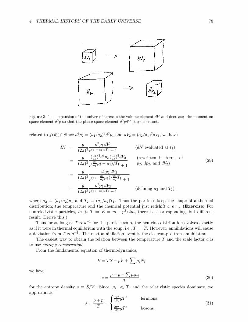
4 THERMAL HISTORY OF THE EARLY UNIVERSE 78

Figure 3: The expansion of the universe increases the volume element dV and decreases the momentumspace element d3p so that the phase space element d3pdV stays constant.

related to f(~p1)? Since d3p2 = (a1/a2)3d3p1 and dV2 = (a2/a1)

3dV1, we have

dN =g

(2π)3d3p1 dV1

e(p1−µ1)/T1 ± 1(dN evaluated at t1)

=g

(2π)3(a2a1 )

3d3p2 (a1a2)3dV2

e(a2a1p2 − µ1)/T1 ± 1

(rewritten in terms ofp2, dp2, and dV2)

(29)

=g

(2π)3d3p2 dV2

e(p2−

a1a2µ1)/

a1a2T1 ± 1

=g

(2π)3d3p2 dV2

e(p2−µ2)/T2 ± 1(defining µ2 and T2) ,

where µ2 ≡ (a1/a2)µ1 and T2 ≡ (a1/a2)T1. Thus the particles keep the shape of a thermaldistribution; the temperature and the chemical potential just redshift ∝ a−1. (Exercise: Fornonrelativistic particles, m ≫ T ⇒ E = m + p2/2m, there is a corresponding, but differentresult. Derive this.)

Thus for as long as T ∝ a−1 for the particle soup, the neutrino distribution evolves exactlyas if it were in thermal equilibrium with the soup, i.e., Tν = T . However, annihilations will causea deviation from T ∝ a−1. The next annihilation event is the electron-positron annihilation.

The easiest way to obtain the relation between the temperature T and the scale factor a isto use entropy conservation.

From the fundamental equation of thermodynamics,

E = TS − pV +∑

µiNi

we have

s =ρ+ p−∑

µini

T, (30)

for the entropy density s ≡ S/V . Since |µi| ≪ T , and the relativistic species dominate, weapproximate

s =ρ+ p

T=

7π2

180 gT3 fermions

2π2

45 gT 3 bosons .(31)

4 THERMAL HISTORY OF THE EARLY UNIVERSE 79

Adding up all the relativistic species and allowing now for the possibility that some speciesmay have a kinetic temperature Ti, which differs from the temperature T of those species whichremain in thermal equilibrium, we get

ρ(T ) =π2

30g∗(T )T

4

s(T ) =2π2

45g∗s(T )T

3 , (32)

where now

g∗(T ) =∑

bos

gi

(

Ti

T

)4

+7

8

∑

fer

gi

(

Ti

T

)4

g∗s(T ) =∑

bos

gi

(

Ti

T

)3

+7

8

∑

fer

gi

(

Ti

T

)3

, (33)

and the sums are over all relativistic species of bosons and fermions.If some species are “semirelativistic”, i.e., m = O(T ), ρ(T ) and s(T ) are to be calculated

from the integral formulae in Sec. 4.1, and Eq. (32) defines g∗(T ) and g∗s(T ).For as long as all species have the same temperature and p ≈ 1

3ρ, we have

g∗s(T ) ≈ g∗(T ). (34)

The electron annihilation, however, forces us to make a distinction between g∗(T ) and g∗s(T ).According to the second law of thermodynamics the total entropy of the universe never

decreases; it either stays constant or increases. An increase in entropy is always related to adeviation from thermodynamic equilibrium. It turns out that any entropy production in thevarious known processes in the universe is totally insignificant compared to the total entropy ofthe universe5, which is huge, and dominated by the relativistic species. Thus it is an excellentapproximation to treat the expansion of the universe as adiabatic, so that the total entropy staysconstant, i.e.,

d(sa3) = 0. (35)

This now gives us the relation between a and T ,

g∗s(T )T3a3 = const. (36)

We shall have much use for this formula.In the electron annihilation g∗s changes from

g∗s = g∗ = 2 + 3.5 + 5.25 = 10.75 (37)

γ e± ν

to

g∗s = 2 + 5.25

(

Tν

T

)3

, (38)

whereT 3ν a

3 = const = T 3a3(before annihilation). (39)

5There may be exceptions to this in the very early universe, most notably inflation, where essentially all theentropy of the universe supposedly was produced.

4 THERMAL HISTORY OF THE EARLY UNIVERSE 80

(since the neutrinos have decoupled, Tν redshifts Tν ∝ a−1). As the number of relativisticdegrees of freedom is reduced, energy density and entropy are transferred from electrons andpositrons to photons, but not to neutrinos, in the annihilation reactions

e+ + e− → γ + γ.

The photons are thus heated (the photon temperature does not fall as much) relative to neutri-nos.

Dividing Eq. (36) with Eq. (39) we get that

g∗s(T )

(

T

Tν

)3

= const

or (Eqs. (37) and (38))

10.75 = 2

(

T

Tν

)3

+ 5.25 (before = after)

from which we solve the neutrino temperature after e+e−-annihilation,

Tν =

(

4

11

)

13T = 0.71377T

g∗s(T ) = 2 + 5.25 · 4

11= 3.909 (40)

g∗(T ) = 2 + 5.25

(

4

11

)

43

= 3.363.

To be more precise, neutrino decoupling was not complete when e+e−-annihilation began;so that some of the energy and entropy leaked to the neutrinos. Therefore the neutrino energydensity after e+e−-annihilation is about 1.5% higher (at a given T ) than the above calculationgives. The neutrino distribution also deviates slightly from kinetic equilibrium. In the above

5.25 =21

4=

7

4Nν , (41)

where Nν = 3 is the number of neutrino species. To correct for the additional energy densitywe define an effective number of neutrino species Neff by

ρν ≡ Neff7

8

(

4

11

)4/3

ργ (42)

after e+e−-annihilation. After many years of hard work by theorists it has been calculated that[3, 4, 5]

Neff ≈ 3.046 . (43)

This replaces 5.25 by 74Neff = 5.3305 in the above, so that

g∗s(T ) = 2 + 5.3305 · 4

11= 3.938

g∗(T ) = 2 + 5.3305

(

4

11

)

43

= 3.384 .

These relations remain true for the photon+neutrino background as long as the neutrinos stayultrarelativistic (mν ≪ T ). It used to be the standard assumption that neutrinos are massless

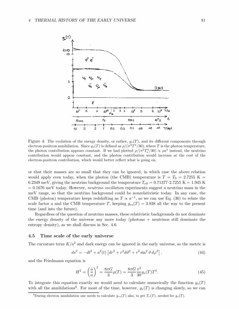
4 THERMAL HISTORY OF THE EARLY UNIVERSE 81

Figure 4: The evolution of the energy density, or rather, g∗(T ), and its different components throughelectron-positron annihilation. Since g∗(T ) is defined as ρ/(π2T 4/30), where T is the photon temperature,the photon contribution appears constant. If we had plotted ρ/(π2T 4

ν /30) ∝ ρa4 instead, the neutrinocontribution would appear constant, and the photon contribution would increase at the cost of theelectron-positron contribution, which would better reflect what is going on.

or that their masses are so small that they can be ignored, in which case the above relationwould apply even today, when the photon (the CMB) temperature is T = T0 = 2.7255 K =0.2349 meV, giving the neutrino background the temperature Tν0 = 0.71377·2.7255 K = 1.945 K= 0.1676 meV today. However, neutrino oscillation experiments suggest a neutrino mass in themeV range, so that the neutrino background could be nonrelativistic today. In any case, theCMB (photon) temperature keeps redshifting as T ∝ a−1, so we can use Eq. (36) to relate thescale factor a and the CMB temperature T , keeping g∗s(T ) = 3.938 all the way to the presenttime (and into the future).

Regardless of the question of neutrino masses, these relativistic backgrounds do not dominatethe energy density of the universe any more today (photons + neutrinos still dominate theentropy density), as we shall discuss in Sec. 4.6.

4.5 Time scale of the early universe

The curvature term K/a2 and dark energy can be ignored in the early universe, so the metric is

ds2 = −dt2 + a2(t)[

dr2 + r2dϑ2 + r2 sin2 ϑ dϕ2]

. (44)

and the Friedmann equation is

H2 =

(

a

a

)2

=8πG

3ρ(T ) =

8πG

3

π2

30g∗(T )T

4. (45)

To integrate this equation exactly we would need to calculate numerically the function g∗(T )with all the annihilations6. For most of the time, however, g∗(T ) is changing slowly, so we can

6During electron annihilation one needs to calculate g∗s(T ) also, to get Tν(T ), needed for g∗(T ).

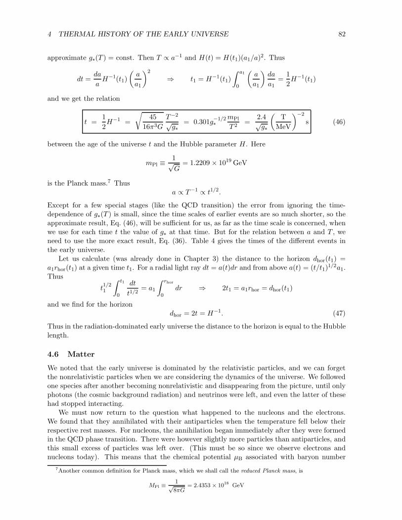
4 THERMAL HISTORY OF THE EARLY UNIVERSE 82

approximate g∗(T ) = const. Then T ∝ a−1 and H(t) = H(t1)(a1/a)2. Thus

dt =da

aH−1(t1)

(

a

a1

)2

⇒ t1 = H−1(t1)

∫ a1

0

(

a

a1

)

da

a1=

1

2H−1(t1)

and we get the relation

t =1

2H−1 =

√

45

16π3G

T−2

√g∗

= 0.301g−1/2∗

mPl

T 2=

2.4√g∗

(

T

MeV

)−2

s (46)

between the age of the universe t and the Hubble parameter H. Here

mPl ≡1√G

= 1.2209 × 1019 GeV

is the Planck mass.7 Thusa ∝ T−1 ∝ t1/2.

Except for a few special stages (like the QCD transition) the error from ignoring the time-dependence of g∗(T ) is small, since the time scales of earlier events are so much shorter, so theapproximate result, Eq. (46), will be sufficient for us, as far as the time scale is concerned, whenwe use for each time t the value of g∗ at that time. But for the relation between a and T , weneed to use the more exact result, Eq. (36). Table 4 gives the times of the different events inthe early universe.

Let us calculate (was already done in Chapter 3) the distance to the horizon dhor(t1) =a1rhor(t1) at a given time t1. For a radial light ray dt = a(t)dr and from above a(t) = (t/t1)

1/2a1.Thus

t1/21

∫ t1

0

dt

t1/2= a1

∫ rhor

0dr ⇒ 2t1 = a1rhor = dhor(t1)

and we find for the horizondhor = 2t = H−1. (47)

Thus in the radiation-dominated early universe the distance to the horizon is equal to the Hubblelength.

4.6 Matter

We noted that the early universe is dominated by the relativistic particles, and we can forgetthe nonrelativistic particles when we are considering the dynamics of the universe. We followedone species after another becoming nonrelativistic and disappearing from the picture, until onlyphotons (the cosmic background radiation) and neutrinos were left, and even the latter of thesehad stopped interacting.

We must now return to the question what happened to the nucleons and the electrons.We found that they annihilated with their antiparticles when the temperature fell below theirrespective rest masses. For nucleons, the annihilation began immediately after they were formedin the QCD phase transition. There were however slightly more particles than antiparticles, andthis small excess of particles was left over. (This must be so since we observe electrons andnucleons today). This means that the chemical potential µB associated with baryon number

7Another common definition for Planck mass, which we shall call the reduced Planck mass, is

MPl ≡1√8πG

= 2.4353 × 1018 GeV

4 THERMAL HISTORY OF THE EARLY UNIVERSE 83

differs from zero (is positive). Baryon number is a conserved quantity. Since nucleons are thelightest baryons, the baryon number resides today in nucleons (protons and neutrons; sincethe proton is lighter than the neutron, free neutrons have decayed into protons, but there areneutrons in atomic nuclei, whose mass/baryon is even smaller). The universe is electricallyneutral, and the negative charge lies in the electrons, the lightest particles with negative charge.Therefore the number of electrons must equal the number of protons.

The number densities etc. of the electrons and the nucleons we get from the equations ofSec. 4.1. But what is the chemical potential µ in them? For each species, we get µ(T ) from theconserved quantities.8 The baryon number resides in the nucleons,

nB = nN − nN = np + nn − np − nn . (48)

Let us define the parameter η, the baryon-photon ratio today,

η ≡ nB(t0)

nγ(t0). (49)

From observations we know that η = 10−10–10−9. Since baryon number is conserved, nBV ∝nBa

3 stays constant, sonB ∝ a−3 . (50)

After electron annihilation nγ ∝ a−3, so we get

nB(T ) = ηnγ = η2ζ(3)

π2T 3 for T ≪ me , (51)

and for all times (as long as the universe expands adiabatically and the baryon number isconserved), using Eqs. (36), (50), and (51),

nB(T ) = η2ζ(3)

π2

g∗s(T )

g∗s(T0)T 3 . (52)

For T < 10 MeV we have in practice

nN ≪ nN and nN ≡ nn + np = nB .

We shall later (Chapter 5) discuss big bang nucleosynthesis—how the protons and neutronsformed atomic nuclei. Approximately one quarter of all nucleons (all neutrons and roughly thesame number of protons) form nuclei (A > 1) and three quarters remain as free protons. Let usdenote by n∗

p and n∗n the number densities of protons and neutrons including those in nuclei (and

also those in atoms), whereas we shall use np and nn for the number densities of free protonsand neutrons. Thus we write instead

n∗

N ≡ n∗

n + n∗

p = nB .

In the same manner, for T < 10 keV we have

ne+ ≪ ne− and ne− = n∗

p .

At this time (T ∼ 10 keV → 1 eV) the universe contains a relativistic photon and neutrinobackground (“radiation”) and nonrelativistic free electrons, protons, and nuclei (“matter”).

8In general, the recipe to find how the thermodynamical parameters, temperature and the chemical poten-tials, evolve in the expanding FRW universe, is to use the conservation laws of the conserved numbers, entropyconservation, and energy continuity, to find how the number densities and energy densities must evolve. Thethermodynamical parameters will then evolve to satisfy these requirements.

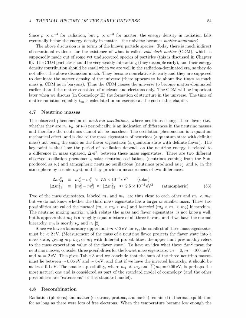
4 THERMAL HISTORY OF THE EARLY UNIVERSE 84

Since ρ ∝ a−4 for radiation, but ρ ∝ a−3 for matter, the energy density in radiation fallseventually below the energy density in matter—the universe becomes matter-dominated.

The above discussion is in terms of the known particle species. Today there is much indirectobservational evidence for the existence of what is called cold dark matter (CDM), which issupposedly made out of some yet undiscovered species of particles (this is discussed in Chapter6). The CDM particles should be very weakly interacting (they decouple early), and their energydensity contribution should be small when we are well in the radiation-dominated era, so they donot affect the above discussion much. They become nonrelativistic early and they are supposedto dominate the matter density of the universe (there appears to be about five times as muchmass in CDM as in baryons). Thus the CDM causes the universe to become matter-dominatedearlier than if the matter consisted of nucleons and electrons only. The CDM will be importantlater when we discuss (in Cosmology II) the formation of structure in the universe. The time ofmatter-radiation equality teq is calculated in an exercise at the end of this chapter.

4.7 Neutrino masses

The observed phenomenon of neutrino oscillations, where neutrinos change their flavor (i.e.,whether they are νe, νµ, or ντ ) periodically, is an indication of differences in the neutrino massesand therefore the neutrinos cannot all be massless. The oscillation phenomenon is a quantummechanical effect, and is due to the mass eigenstates of neutrinos (a quantum state with definitemass) not being the same as the flavor eigenstates (a quantum state with definite flavor). Thekey point is that how the period of oscillation depends on the neutrino energy is related toa difference in mass squared, ∆m2, between these mass eigenstates. There are two differentobserved oscillation phenomena, solar neutrino oscillations (neutrinos coming from the Sun,produced as νe) and atmospheric neutrino oscillations (neutrinos produced as νµ and νe in theatmosphere by cosmic rays), and they provide a measurement of two differences:

∆m221 ≡ m2

2 −m21 ≈ 7.5× 10−5 eV2 (solar)

|∆m231| ≡ |m2

3 −m21| ≈ |∆m2

32| ≈ 2.5 × 10−3 eV2 (atmospheric) . (53)

Two of the mass eigenstates, labeled m1 and m2, are thus close to each other and m1 < m2;but we do not know whether the third mass eigenstate has a larger or smaller mass. These twopossibilities are called the normal (m1 < m2 < m3) and inverted (m3 < m1 < m2) hierarchies.The neutrino mixing matrix, which relates the mass and flavor eigenstates, is not known well,but it appears that m2 is a roughly equal mixture of all three flavors, and if we have the normalhierarchy, m3 is mostly νµ and ντ .[2]

Since we have a laboratory upper limit m < 2 eV for νe, the smallest of these mass eigenstatesmust be < 2 eV. (Measurement of the mass of a neutrino flavor projects the flavor state into amass state, giving m1, m2, or m3 with different probabilities; the upper limit presumably refersto the mass expectation value of the flavor state.) To have an idea what these ∆m2 mean forneutrino masses, consider three possibilities for the lowest mass eigenstate: m = 0, m = 100meV,and m = 2 eV. This gives Table 3 and we conclude that the sum of the three neutrino massesmust lie between ∼ 0.06 eV and ∼ 6 eV, and that if we have the inverted hierarchy, it should beat least 0.1 eV. The smallest possibility, where m1 ≪ m2 and

∑

mi = 0.06 eV, is perhaps themost natural one and is considered as part of the standard model of cosmology (and the otherpossibilities are “extensions” of this standard model).

4.8 Recombination

Radiation (photons) and matter (electrons, protons, and nuclei) remained in thermal equilibriumfor as long as there were lots of free electrons. When the temperature became low enough the

4 THERMAL HISTORY OF THE EARLY UNIVERSE 85

Normal Invertedm1 m2 m3

∑

mi m3 m1 m2∑

mi

0 8.7meV 50meV 59meV 0 50meV 50.7meV 101meV100meV 100.4meV 112meV 312meV 100meV 111.8meV 112.1meV 324meV2 eV 2 eV 2 eV 6 eV 2 eV 2 eV 2 eV 6 eV

Table 3: Possibilities for neutrino masses.

electrons and nuclei combined to form neutral atoms (recombination), and the density of freeelectrons fell sharply. The photon mean free path grew rapidly and became longer than thehorizon distance. Thus the universe became transparent. Photons and matter decoupled, i.e.,their interaction was no more able to maintain them in thermal equilibrium with each other.After this, by T we refer to the photon temperature. Today, these photons are the CMB,and T = T0 = 2.7255K. (After photon decoupling, the matter temperature fell at first fasterthan the photon temperature, but structure formation then heated up the matter to differenttemperatures at different places.)

To simplify the discussion of recombination, let us forget other nuclei than protons (in realityover 90% (by number) of the nuclei are protons, and almost all the rest are 4He nuclei). Letus denote the number density of free protons by np, free electrons by ne, and hydrogen atomsby nH. Since the universe is electrically neutral, np = ne. The conservation of baryon numbergives nB = np + nH. From Sec. 4.1 we have

ni = gi

(

miT

2π

)3/2

eµi−mi

T . (54)

For as long as the reactionp+ e− ↔ H+ γ (55)

is in chemical equilibrium the chemical potentials are related by µp + µe = µH (since µγ = 0).Using this we get the relation

nH =gHgpge

npne

(

meT

2π

)−3/2

eB/T , (56)

between the number densities. Here B = mp + me − mH = 13.6 eV is the binding energy ofhydrogen. The numbers of internal degrees of freedom are gp = ge = 2, gH = 4. Outside theexponent we approximated mH ≈ mp. Defining the fractional ionization

x ≡ np

nB⇒ nH

npne=

(1− x)

x2nB. (57)

Using (51), Eq. (56) becomes

1− x

x2=

4√2 ζ(3)√π

η

(

T

me

)3/2

eB/T , (58)

the Saha equation for ionization in thermal equilibrium. When B ≪ T ≪ me, the RHS ≪ 1 sothat x ∼ 1, and almost all protons and electrons are free. As temperature falls, eB/T grows, butsince both η and (T/me)

3/2 are ≪ 1, the temperature needs to fall to T ≪ B, before the wholeexpression becomes large (∼ 1 or ≫ 1).

The ionization fraction at first follows the equilibrium result of Eq. (58) closely, but as thisequilibrium fraction begins to fall rapidly, the true ionization fraction begins to lag behind. As

4 THERMAL HISTORY OF THE EARLY UNIVERSE 86

0 0

0.2 0.2

0.4 0.4

0.6 0.6

0.8 0.8

1 1

x

SahaPeebles

90010001100120013001400150016001700180019001+z

1e+05

1e+06

1e+07

1e+08

1e+09

n e/m-3

90010001100120013001400150016001700180019001+z

0.1

1

10

100

1000

λ γ/Mpc

ne/m

-3

λγ/Mpc

Figure 5: Recombination. In the top panel the dashed curve gives the equilibrium ionization fraction asgiven by the Saha equation. The solid curve is the true ionization fraction, calculated using the actualreaction rates (original calculation by Peebles). You can see that the equilibrium fraction is followed atfirst, but then the true fraction lags behind. The bottom panel shows the free electron number densityne and the photon mean free path λγ . The latter is given in comoving units, i.e., the distance is scaledto the corresponding present distance. This figure is for η = 8.22× 10−10. (Figure by R. Keskitalo.)

the number densities of free electrons and protons fall, it becomes more difficult for them to findeach other to “recombine”, and they are no longer able to maintain chemical equilibrium for thereaction (55). To find the correct ionization evolution, x(t), requires then a more complicatedcalculation involving the reaction cross section of this reaction. See Figs. 5 and 6.

Although the equilibrium formula is thus not enough to give us the true ionization evolution,its benefit is twofold:

1. It tells us when recombination begins. While the equilibrium ionization changes slowly,it is easy to stay in equilibrium. Thus things won’t start to happen until the equilibriumfraction begins to change a lot.

2. It gives the initial conditions for the more complicated calculation that will give the trueevolution.

A similar situation holds for many other events in the early universe, e.g., big bang nucleosyn-thesis.

The recombination is not instantaneous. Let us define the recombination temperature Trec

as the temperature where x = 0.5. Now Trec = T0(1 + zrec) since 1 + z = a−1 and the photontemperature falls as T ∝ a−1. (Since η ≪ 1, the energy release in recombination is negli-gible compared to ργ ; and after photon decoupling photons travel freely maintaining kineticequilibrium with T ∝ a−1.)

We get (for η ∼ 10−9)

Trec ∼ 0.3 eV

zrec ∼ 1300.

You might have expected that Trec ∼ B. Instead we found Trec ≪ B. The main reason for this isthat η ≪ 1. This means that there are very many photons for each hydrogen atom. Even when

4 THERMAL HISTORY OF THE EARLY UNIVERSE 87

1e-05 1e-05

0.0001 0.0001

0.001 0.001

0.01 0.01

0.1 0.1

1 1

10 10

x

SahaPeebles

0200400600800100012001400160018001+z

0.0001

0.01

1

100

10000

1e+06

1e+08

n e/m-3

0200400600800100012001400160018001+z

0.01

1

100

10000

1e+06

1e+08

1e+10

λ γ/Mpc

ne/m

-3

λγ/Mpc

Figure 6: Same as Fig. 5, but with a logarithmic scale for the ionization fraction, and the time (actuallyredshift) scale extended to present time (z = 0 or 1 + z = 1). You can see how a residual ionizationx ∼ 10−4 remains. This figure does not include the reionization which happened at around z ∼ 10.(Figure by R. Keskitalo.)

T ≪ B, the high-energy tail of the photon distribution contains photons with energy E > B sothat they can ionize a hydrogen atom.

The photon decoupling takes place somewhat later, at Tdec ≡ (1+zdec)T0, when the ionizationfraction has fallen enough. We define the photon decoupling time to be the time when the photonmean free path exceeds the Hubble distance. The numbers are

Tdec ≈ 2974K ∼ 0.256 eV

zdec ≈ 1090.

The decoupling means that the recombination reaction can not keep the ionization fraction onthe equilibrium track, but instead we are left with a residual ionization of x ∼ 10−4.

A long time later (z ∼ 10) the first stars form, and their radiation reionizes the gas that isleft in interstellar space. The gas has now such a low density however, that the universe remainstransparent.

Exercise: Transparency of the universe. We say the universe is transparent when the photonmean free path λγ is larger than the Hubble length lH = H−1, and opaque when λγ < lH . The photonmean free path is determined mainly by the scattering of photons by free electrons, so that λγ = 1/(σTne),where ne = xn∗

e is the number density of free electrons, n∗

e is the total number density of electrons, andx is the ionization fraction. The cross section for photon-electron scattering is independent of energyfor Eγ ≪ me and is then called the Thomson cross section, σT = 8π

3(α/me)

2, where α is the fine-structure constant. In recombination x falls from 1 to 10−4. Show that the universe is opaque beforerecombination and transparent after recombination. (Assume the recombination takes place betweenz = 1300 and z = 1000. You can assume a matter-dominated universe—see below for parameter values.)The interstellar matter gets later reionized (to x ∼ 1) by the light from the first stars. What is the earliestredshift when this can happen without making the universe opaque again? (You can assume that most(∼ all) matter has remained interstellar). Calculate for Ωm = 1.0 and Ωm = 0.3 (note that Ωm includesnonbaryonic matter). Use ΩΛ = 0, h = 0.7 and η = 6× 10−10.

The photons in the cosmic background radiation have thus traveled without scatteringthrough space all the way since we had T = Tdec = 1091T0. When we look at this cosmic

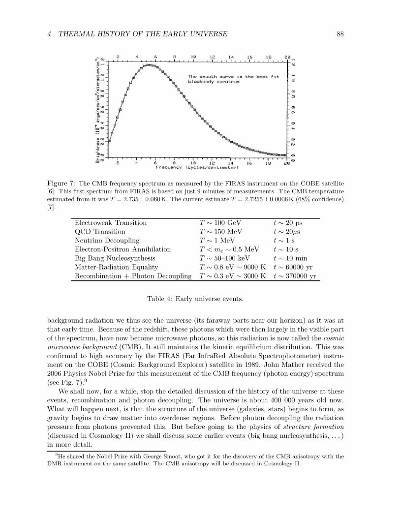
4 THERMAL HISTORY OF THE EARLY UNIVERSE 88

Figure 7: The CMB frequency spectrum as measured by the FIRAS instrument on the COBE satellite[6]. This first spectrum from FIRAS is based on just 9 minutes of measurements. The CMB temperatureestimated from it was T = 2.735±0.060K. The current estimate T = 2.7255±0.0006K (68% confidence)[7].

Electroweak Transition T ∼ 100 GeV t ∼ 20 psQCD Transition T ∼ 150 MeV t ∼ 20µsNeutrino Decoupling T ∼ 1 MeV t ∼ 1 sElectron-Positron Annihilation T < me ∼ 0.5 MeV t ∼ 10 sBig Bang Nucleosynthesis T ∼ 50–100 keV t ∼ 10 minMatter-Radiation Equality T ∼ 0.8 eV ∼ 9000 K t ∼ 60000 yrRecombination + Photon Decoupling T ∼ 0.3 eV ∼ 3000 K t ∼ 370000 yr

Table 4: Early universe events.

background radiation we thus see the universe (its faraway parts near our horizon) as it was atthat early time. Because of the redshift, these photons which were then largely in the visible partof the spectrum, have now become microwave photons, so this radiation is now called the cosmic

microwave background (CMB). It still maintains the kinetic equilibrium distribution. This wasconfirmed to high accuracy by the FIRAS (Far InfraRed Absolute Spectrophotometer) instru-ment on the COBE (Cosmic Background Explorer) satellite in 1989. John Mather received the2006 Physics Nobel Prize for this measurement of the CMB frequency (photon energy) spectrum(see Fig. 7).9

We shall now, for a while, stop the detailed discussion of the history of the universe at theseevents, recombination and photon decoupling. The universe is about 400 000 years old now.What will happen next, is that the structure of the universe (galaxies, stars) begins to form, asgravity begins to draw matter into overdense regions. Before photon decoupling the radiationpressure from photons prevented this. But before going to the physics of structure formation

(discussed in Cosmology II) we shall discuss some earlier events (big bang nucleosynthesis, . . . )in more detail.

9He shared the Nobel Prize with George Smoot, who got it for the discovery of the CMB anisotropy with theDMR instrument on the same satellite. The CMB anisotropy will be discussed in Cosmology II.

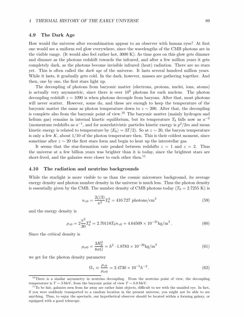
4 THERMAL HISTORY OF THE EARLY UNIVERSE 89

4.9 The Dark Age

How would the universe after recombination appear to an observer with human eyes? At firstone would see a uniform red glow everywhere, since the wavelengths of the CMB photons are inthe visible range. (It would also feel rather hot, 3000 K). As time goes on this glow gets dimmerand dimmer as the photons redshift towards the infrared, and after a few million years it getscompletely dark, as the photons become invisible infrared (heat) radiation. There are no starsyet. This is often called the dark age of the universe. It lasts several hundred million years.While it lasts, it gradually gets cold. In the dark, however, masses are gathering together. Andthen, one by one, the first stars light up.

The decoupling of photons from baryonic matter (electrons, protons, nuclei, ions, atoms)is actually very asymmetric, since there is over 109 photons for each nucleus. The photondecoupling redshift z = 1090 is when photons decouple from baryons. After that, most photonswill never scatter. However, some do, and these are enough to keep the temperature of thebaryonic matter the same as photon temperature down to z ∼ 200. After that, the decouplingis complete also from the baryonic point of view.10 The baryonic matter (mainly hydrogen andhelium gas) remains in internal kinetic equilibrium, but its temperature Tb falls now as a−2

(momentum redshifts as a−1, and for nonrelativistic particles kinetic energy is p2/2m and meankinetic energy is related to temperature by 〈Ek〉 = 3T/2). So at z ∼ 20, the baryon temperatureis only a few K, about 1/10 of the photon temperature then. This is their coldest moment, sincesometime after z ∼ 20 the first stars form and begin to heat up the interstellar gas.

It seems that the star-formation rate peaked between redshifts z = 1 and z = 2. Thusthe universe at a few billion years was brighter than it is today, since the brightest stars areshort-lived, and the galaxies were closer to each other then.11

4.10 The radiation and neutrino backgrounds

While the starlight is more visible to us than the cosmic microwave background, its averageenergy density and photon number density in the universe is much less. Thus the photon densityis essentially given by the CMB. The number density of CMB photons today (T0 = 2.7255 K) is

nγ0 =2ζ(3)

π2T 30 = 410.727 photons/cm3 (59)

and the energy density is

ργ0 = 2π2

30T 40 = 2.70118T0nγ0 = 4.64509 × 10−31kg/m3 . (60)

Since the critical density is

ρcr0 =3H2

0

8πG= h2 · 1.8783 × 10−26kg/m3 (61)

we get for the photon density parameter

Ωγ ≡ ργ0ρcr0

= 2.4730 × 10−5h−2 . (62)

10There is a similar asymmetry in neutrino decoupling. From the neutrino point of view, the decouplingtemperature is T ∼ 3MeV, from the baryonic point of view T ∼ 0.8MeV.

11To be fair, galaxies seen from far away are rather faint objects, difficult to see with the unaided eye. In fact,if you were suddenly transported to a random location in the present universe, you might not be able to seeanything. Thus, to enjoy the spectacle, our hypothetical observer should be located within a forming galaxy, orequipped with a good telescope.

4 THERMAL HISTORY OF THE EARLY UNIVERSE 90

While relativistic, neutrinos contribute another radiation component

ρν =7Neff

4

π2

30T 4ν . (63)

After e+e−-annihilation this gives

ρν =7Neff

8

(

4

11

)4

3

ργ , (64)

where Neff = 3.046 is the effective number of neutrino species.When the number of neutrino species was not yet known, cosmology (BBN) was used to

constrain it. Big bang nucleosynthesis is sensitive to the expansion rate in the early universe,and that depends on the energy density. Observations of abundances of light element isotopescombined with BBN calculations require Neff = 2–4. Actually any new light particle species thatwould be relativistic at nucleosynthesis time (T ∼ 50 keV – 1 MeV) and would thus contributeto the expansion rate through its energy density, but which would not interact directly withnuclei and electrons, would have the same effect. Thus such hypothetical unknown particles(called dark radiation) may not contribute to the energy density of the universe at that timemore than one neutrino species does.

If neutrinos are still relativistic today, the neutrino density parameter is

Ων =7Neff

8

(

4

11

)4

3

Ωγ = 0.6918Ωγ = 1.7107 × 10−5h−2 , (65)

so that the total radiation density parameter is

Ωr = Ωγ +Ων = 4.1837 × 10−5h−2 ∼ 10−4 . (66)

We thus confirm the claim in Chapter 3, that the radiation component can be ignored in theFriedmann equation, except in the early universe. The combination Ωih

2 is often denoted byωi, so we have

ωγ = 2.4730 × 10−5 (67)

ων = 1.7107 × 10−5 (68)

ωr = ωγ + ων = 4.1837 × 10−5 . (69)

Neutrino oscillation experiments indicate a neutrino mass in the meV–eV range. This meansthat neutrinos are nonrelativistic today and count as matter, not radiation, except possibly thelightest neutrino species. Then the above result for the neutrino energy density of the presentuniverse does not apply. However, unless the neutrino masses are above 0.2 eV, they wouldstill have been relativistic, and counted as radiation, at the time of recombination and matter-radiation equality. While the neutrinos are relativistic, one still gets the neutrino energy densityas

ρν = Ωνρcr0a−4 (70)

using the Ων of Eq. (65), even though this relation does not hold when the neutrinos becomenonrelativistic and thus this Ων is not the density parameter to give the present density ofneutrinos (we shall discuss that in Chapter 6).

Exercise: Matter–radiation equality. The present density of matter is ρm0 = Ωmρcr0 and thepresent density of radiation is ρr0 = ργ0 + ρν0 (we assume neutrinos are massless). What was the ageof the universe teq when ρm = ρr? (Note that in these early times—but not today—you can ignore thecurvature and vacuum terms in the Friedmann equation.) Give numerical value (in years) for the casesΩm = 0.1, 0.3, and 1.0, and H0 = 70km/s/Mpc. What was the temperature (Teq) then?

REFERENCES 91

References

[1] H. Waltari, private communication (2016)

[2] K. Huitu, private communication (2017)

[3] G. Mangano et al., A precision calculation of the effective number of cosmological neutrinos,Phys. Lett. B 534, 8 (2002)

[4] P.F. de Salas and S. Pastor, Relic neutrino decoupling with flavour oscillations revisited,JCAP 07, 051 (2016), arXiv:1606.06986

[5] Planck Collaboration, Planck 2018 results. VI. Cosmological parameters,arXiv:1807.06209v1

[6] J.C. Mather et al., Astrophys. J. Lett. 354, 37 (1990)

[7] D.J. Fixsen, The Temperature of the Cosmic Microwave Background, Astrophys. J. 707,916 (2009)

5 Big Bang Nucleosynthesis

One quarter (by mass) of the baryonic matter in the universe is helium. Heavier elements makeup a few per cent. The rest, i.e., the major part, is hydrogen.

The building blocks of atomic nuclei, the nucleons, or protons and neutrons, formed in theQCD transition at T ∼ 150MeV and t ∼ 20µs. The protons are hydrogen (1H) nuclei.

Elements (their nuclei) heavier than helium, and also some of the helium, have mostly beenproduced by stars in different processes (see Fig. 1). However, the amount of helium and thepresence of significant amounts of the heavier hydrogen isotope, deuterium (2H), in the universecannot be understood by these astrophysical mechanisms. It turns out that 2H, 3He, 4He, anda significant part of 7Li, were mainly produced already in the big bang, in a process we call BigBang Nucleosynthesis (BBN).

The nucleons and antinucleons annihilated each other soon after the QCD transition, andthe small excess of nucleons left over from annihilation did not have a significant effect on theexpansion and thermodynamics of the universe until much later (t ∼ teq = Ω−2

m h−41000 a), whenthe universe became matter-dominated. The ordinary matter in the present universe comes fromthis small excess of nucleons. Let us now consider what happened to it in the early universe. Weshall focus on the period when the temperature fell from T ∼ 10MeV to T ∼ 10 keV (t ∼ 10ms– few h).

5.1 Equilibrium

The total number of nucleons stays constant due to baryon number conservation. This baryonnumber can be in the form of protons and neutrons or atomic nuclei. Weak nuclear reactionsmay convert neutrons and protons into each other and strong nuclear reactions may build nucleifrom them.

During the period of interest the nucleons and nuclei are nonrelativistic (T ≪ mp). Assumingthermal equilibrium we have

ni = gi

(

miT

2π

)3/2

eµi−mi

T (1)

for the number density of nucleus type i. If the nuclear reactions needed to build nucleus i (withmass number A and charge Z) from the nucleons,

(A− Z)n + Zp ↔ i ,

occur at sufficiently high rate to maintain chemical equilibrium, we have

µi = (A− Z)µn + Zµp (2)

for the chemical potentials. Since for free nucleons

np = 2

(

mpT

2π

)3/2

eµp−mp

T

nn = 2

(

mnT

2π

)3/2

eµn−mn

T , (3)

we can express ni in terms of the neutron and proton densities,

ni = giA32 2−A

(

2π

mNT

)32(A−1)

nZp n

A−Zn eBi/T , (4)

whereBi ≡ (A− Z)mn + Zmp −mi (5)

92

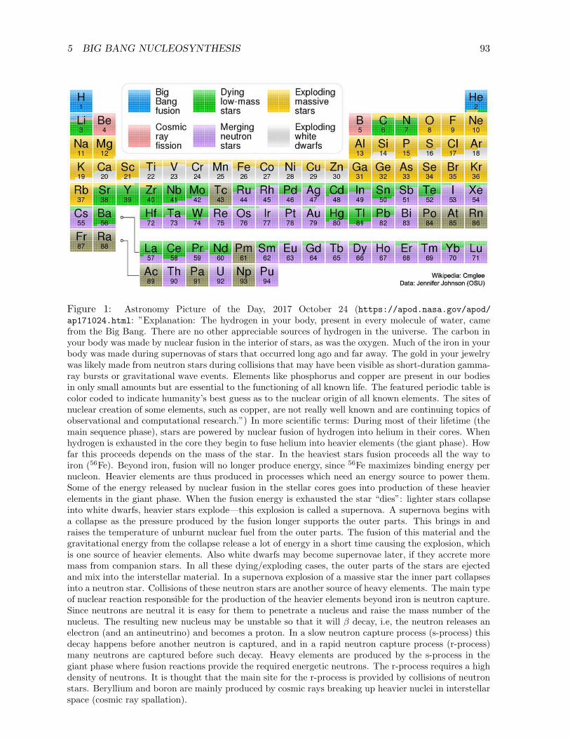
5 BIG BANG NUCLEOSYNTHESIS 93

Figure 1: Astronomy Picture of the Day, 2017 October 24 (https://apod.nasa.gov/apod/ap171024.html: ”Explanation: The hydrogen in your body, present in every molecule of water, camefrom the Big Bang. There are no other appreciable sources of hydrogen in the universe. The carbon inyour body was made by nuclear fusion in the interior of stars, as was the oxygen. Much of the iron in yourbody was made during supernovas of stars that occurred long ago and far away. The gold in your jewelrywas likely made from neutron stars during collisions that may have been visible as short-duration gamma-ray bursts or gravitational wave events. Elements like phosphorus and copper are present in our bodiesin only small amounts but are essential to the functioning of all known life. The featured periodic table iscolor coded to indicate humanity’s best guess as to the nuclear origin of all known elements. The sites ofnuclear creation of some elements, such as copper, are not really well known and are continuing topics ofobservational and computational research.”) In more scientific terms: During most of their lifetime (themain sequence phase), stars are powered by nuclear fusion of hydrogen into helium in their cores. Whenhydrogen is exhausted in the core they begin to fuse helium into heavier elements (the giant phase). Howfar this proceeds depends on the mass of the star. In the heaviest stars fusion proceeds all the way toiron (56Fe). Beyond iron, fusion will no longer produce energy, since 56Fe maximizes binding energy pernucleon. Heavier elements are thus produced in processes which need an energy source to power them.Some of the energy released by nuclear fusion in the stellar cores goes into production of these heavierelements in the giant phase. When the fusion energy is exhausted the star “dies”: lighter stars collapseinto white dwarfs, heavier stars explode—this explosion is called a supernova. A supernova begins witha collapse as the pressure produced by the fusion longer supports the outer parts. This brings in andraises the temperature of unburnt nuclear fuel from the outer parts. The fusion of this material and thegravitational energy from the collapse release a lot of energy in a short time causing the explosion, whichis one source of heavier elements. Also white dwarfs may become supernovae later, if they accrete moremass from companion stars. In all these dying/exploding cases, the outer parts of the stars are ejectedand mix into the interstellar material. In a supernova explosion of a massive star the inner part collapsesinto a neutron star. Collisions of these neutron stars are another source of heavy elements. The main typeof nuclear reaction responsible for the production of the heavier elements beyond iron is neutron capture.Since neutrons are neutral it is easy for them to penetrate a nucleus and raise the mass number of thenucleus. The resulting new nucleus may be unstable so that it will β decay, i.e, the neutron releases anelectron (and an antineutrino) and becomes a proton. In a slow neutron capture process (s-process) thisdecay happens before another neutron is captured, and in a rapid neutron capture process (r-process)many neutrons are captured before such decay. Heavy elements are produced by the s-process in thegiant phase where fusion reactions provide the required energetic neutrons. The r-process requires a highdensity of neutrons. It is thought that the main site for the r-process is provided by collisions of neutronstars. Beryllium and boron are mainly produced by cosmic rays breaking up heavier nuclei in interstellarspace (cosmic ray spallation).

5 BIG BANG NUCLEOSYNTHESIS 94

is the binding energy of the nucleus. Here we have approximated mp ≈ mn ≈ mi/A outside theexponent, and denoted it by mN (“nucleon mass”).

AZ B(MeV) B/A(MeV) g

2H 2.2245 1.11 33H 8.4820 2.83 23He 7.7186 2.57 24He 28.2970 7.07 16Li 31.9965 5.33 37Li 39.2460 5.61 47Be 37.6026 5.37 1

12C 92.1631 7.68 156Fe 492.2623 8.79 1

Table 1. Some of the lightest nuclei (+ iron) and their binding energies.

The different number densities add up to the total baryon number density∑

Aini = nB . (6)

The baryon number density nB can be expressed in terms of photon density

nγ =2

π2ζ(3)T 3 (7)

and the baryon/photon -rationB

nγ=

g∗s(T )

g∗s(T0)η (8)

as

nB =g∗s(T )

g∗s(T0)η2

π2ζ(3)T 3. (9)

After electron-positron annihilation g∗s(T ) = g∗s(T0) and nB = ηnγ . Here η is the presentbaryon/photon ratio. It can be estimated from various observations in a number of ways. It’sorder of magnitude is 10−9.

We define the mass fraction of nucleus i as

Xi ≡Aini

nBso that

∑

Xi = 1 . (10)

The equilibrium mass fractions are, from Eq. (4),

Xi =1

2XZ

p XA−Zn giA

52 ǫA−1eBi/T (11)

where

ǫ ≡1

2

(

2π

mNT

)3/2

nB =1

π2ζ(3)

(

2πT

mN

)3/2 g∗s(T )

g∗s(T0)η ∼

(

T

mN

)3/2

η.

The factors which change rapidly with T are ǫA−1eBi/T . For temperatures mN ≫ T & Bi wehave eBi/T ∼ 1 and ǫ ≪ 1. Thus Xi ≪ 1 for others (A > 1) than protons and neutrons. Astemperature falls, ǫ becomes even smaller and at T ∼ Bi we have Xi ≪ 1 still. The temperaturehas to fall below Bi by a large factor before the factor eBi/T wins and the equilibrium abundancebecomes large. We calculate below that, e.g., for 4He this happens at T ∼ 0.3MeV, and for 2Hat T ∼ 0.07MeV. Thus we have initially only free neutrons and protons in large numbers.

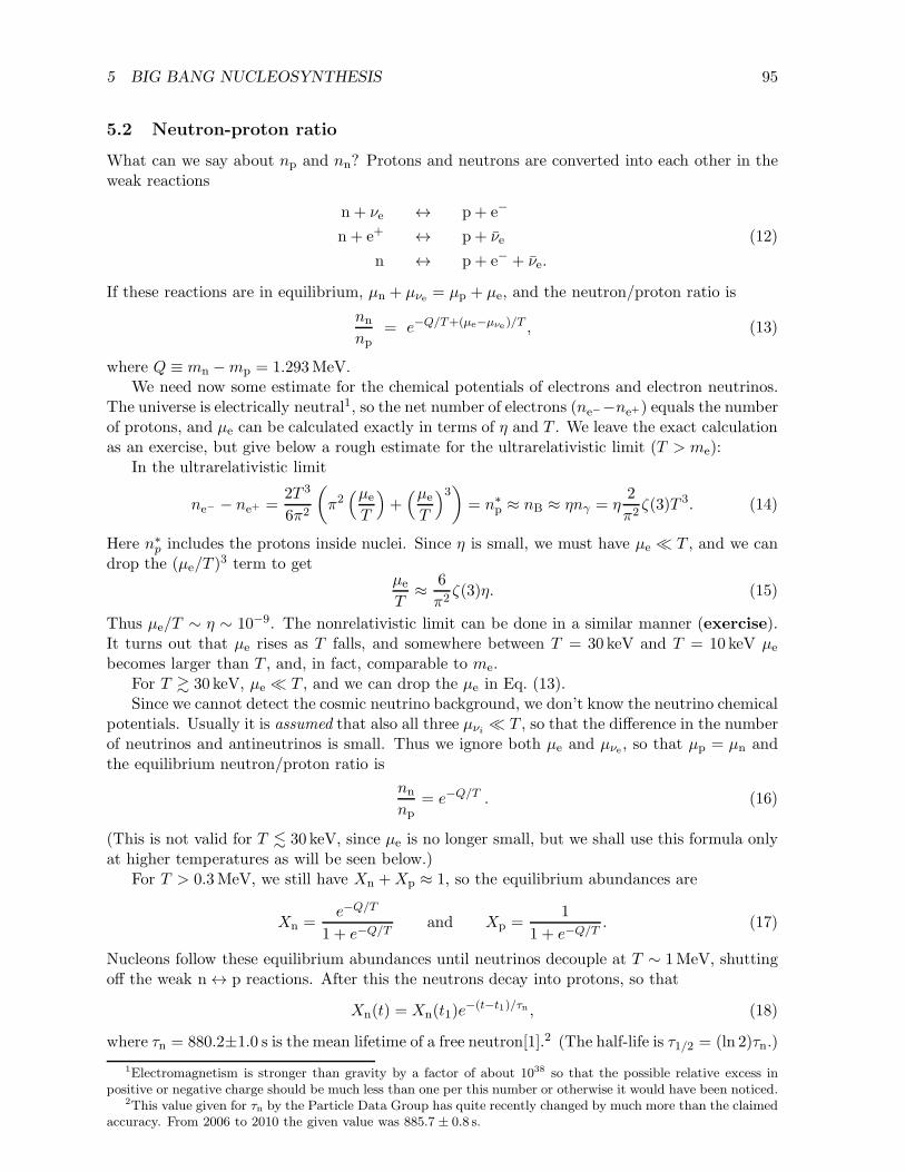
5 BIG BANG NUCLEOSYNTHESIS 95

5.2 Neutron-proton ratio

What can we say about np and nn? Protons and neutrons are converted into each other in theweak reactions

n + νe ↔ p + e−

n + e+ ↔ p + νe (12)

n ↔ p + e− + νe.

If these reactions are in equilibrium, µn + µνe = µp + µe, and the neutron/proton ratio is

nn

np= e−Q/T+(µe−µνe )/T , (13)

where Q ≡ mn −mp = 1.293MeV.We need now some estimate for the chemical potentials of electrons and electron neutrinos.

The universe is electrically neutral1, so the net number of electrons (ne−−ne+) equals the numberof protons, and µe can be calculated exactly in terms of η and T . We leave the exact calculationas an exercise, but give below a rough estimate for the ultrarelativistic limit (T > me):

In the ultrarelativistic limit

ne− − ne+ =2T 3

6π2

(

π2(µe

T

)

+(µe

T

)3)

= n∗

p ≈ nB ≈ ηnγ = η2

π2ζ(3)T 3. (14)

Here n∗

p includes the protons inside nuclei. Since η is small, we must have µe ≪ T , and we candrop the (µe/T )

3 term to getµe

T≈

6

π2ζ(3)η. (15)

Thus µe/T ∼ η ∼ 10−9. The nonrelativistic limit can be done in a similar manner (exercise).It turns out that µe rises as T falls, and somewhere between T = 30 keV and T = 10 keV µe

becomes larger than T , and, in fact, comparable to me.For T & 30 keV, µe ≪ T , and we can drop the µe in Eq. (13).Since we cannot detect the cosmic neutrino background, we don’t know the neutrino chemical

potentials. Usually it is assumed that also all three µνi ≪ T , so that the difference in the numberof neutrinos and antineutrinos is small. Thus we ignore both µe and µνe , so that µp = µn andthe equilibrium neutron/proton ratio is

nn

np= e−Q/T . (16)

(This is not valid for T . 30 keV, since µe is no longer small, but we shall use this formula onlyat higher temperatures as will be seen below.)

For T > 0.3MeV, we still have Xn +Xp ≈ 1, so the equilibrium abundances are

Xn =e−Q/T

1 + e−Q/Tand Xp =

1

1 + e−Q/T. (17)

Nucleons follow these equilibrium abundances until neutrinos decouple at T ∼ 1MeV, shuttingoff the weak n ↔ p reactions. After this the neutrons decay into protons, so that

Xn(t) = Xn(t1)e−(t−t1)/τn , (18)

where τn = 880.2±1.0 s is the mean lifetime of a free neutron[1].2 (The half-life is τ1/2 = (ln 2)τn.)

1Electromagnetism is stronger than gravity by a factor of about 1038 so that the possible relative excess inpositive or negative charge should be much less than one per this number or otherwise it would have been noticed.

2This value given for τn by the Particle Data Group has quite recently changed by much more than the claimedaccuracy. From 2006 to 2010 the given value was 885.7 ± 0.8 s.

5 BIG BANG NUCLEOSYNTHESIS 96

5.3 Bottlenecks

Using (4), (16), and (6)3, we get all equilibrium abundances as a function of T (they also dependon the value of the parameter η). There are two items to note, however:

1. The normalization condition, Eq. (6), includes all nuclei up to uranium etc. Thus we wouldget a huge polynomial equation from which to solve Xp. (After one has Xp, one gets therest easily from (4) and (16).)

2. In practice we don’t have to care about the first item, since as the temperature falls thenuclei no longer follow their equilibrium abundances. The reactions are in equilibriumonly at high temperatures, when the other equilibrium abundances except Xp and Xn aresmall, and we can use the approximation Xn +Xp = 1.

In the early universe the baryon density is too low and the time available is too short forreactions involving three or more incoming nuclei to occur at any appreciable rate. The heaviernuclei have to be built sequentially from lighter nuclei in two-particle reactions, so that deuteriumis formed first in the reaction

n + p → d + γ.

Only when deuterons are available can helium nuclei be formed, and so on. This process has“bottlenecks”: the lack of sufficient densities of lighter nuclei hinders the production of heaviernuclei, and prevents them from following their equilibrium abundances.

As the temperature falls, the equilibrium abundances rise fast. They become large laterfor nuclei with small binding energies. Since deuterium is formed directly from neutrons andprotons it can follow its equilibrium abundance as long as there are large numbers of free neutronsavailable. Since the deuterium binding energy is rather small, the deuterium abundance becomeslarge rather late (at T < 100 keV). Therefore heavier nuclei with larger binding energies, whoseequilibrium abundances would become large earlier, cannot be formed. This is the deuteriumbottleneck. Only when there is lots of deuterium (Xd ∼ 10−3), can helium be produced in largenumbers.

The nuclei are positively charged and there is thus an electromagnetic repulsion betweenthem. The nuclei need thus large kinetic energies to overcome this Coulomb barrier and getwithin the range of the strong interaction. Thus the cross sections for these fusion reactions fallrapidly with energy and the nuclear reactions are “shut off” when the temperature falls belowT ∼ 30 keV. Thus there is less than one hour available for nucleosynthesis. Because of additionalbottlenecks (e.g., there are no stable nuclei with A = 8) and the short time available, only verysmall amounts of elements heavier than helium are formed.

5.4 Calculation of the helium abundance

Let us now calculate the numbers. We saw that because of the deuterium bottleneck, Xn+Xp ≈ 1holds until T ∼ 0.1MeV. Until then, we get Xn and Xp at first from (17) and then from (18).In reality, neutrino decoupling and thus the shift from behavior (17) to behavior (18) is notinstantaneous, but an approximation where one takes it to be instantaneous at time t1 whenT = 0.8MeV, so that Xn(t1) = 0.1657, gives a fairly accurate final result.

Deuterium has Bd = 2.22MeV, and we get ǫeBd/T = 1 at Td = 0.06MeV–0.07MeV (assum-ing η = 10−10 − 10−8), so the deuterium abundance becomes large near this temperature. Since4He has a much higher binding energy, B4 = 28.3MeV, the corresponding situation ǫ3eB4/T = 1occurs at a higher temperature T4 ∼ 0.3MeV. But we noted earlier that only deuterium stays

3For np and nn we know just their ratio, since we do not know µp and µn, only that µp = µn. Therefore thisextra equation is needed to solve all ni.

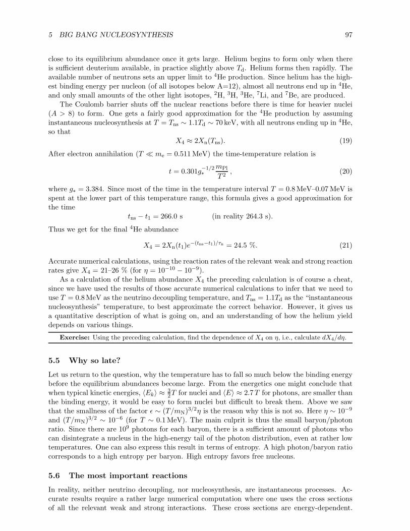
5 BIG BANG NUCLEOSYNTHESIS 97

close to its equilibrium abundance once it gets large. Helium begins to form only when thereis sufficient deuterium available, in practice slightly above Td. Helium forms then rapidly. Theavailable number of neutrons sets an upper limit to 4He production. Since helium has the high-est binding energy per nucleon (of all isotopes below A=12), almost all neutrons end up in 4He,and only small amounts of the other light isotopes, 2H, 3H, 3He, 7Li, and 7Be, are produced.

The Coulomb barrier shuts off the nuclear reactions before there is time for heavier nuclei(A > 8) to form. One gets a fairly good approximation for the 4He production by assuminginstantaneous nucleosynthesis at T = Tns ∼ 1.1Td ∼ 70 keV, with all neutrons ending up in 4He,so that

X4 ≈ 2Xn(Tns). (19)

After electron annihilation (T ≪ me = 0.511MeV) the time-temperature relation is

t = 0.301g−1/2∗

mPl

T 2, (20)

where g∗ = 3.384. Since most of the time in the temperature interval T = 0.8MeV–0.07MeV isspent at the lower part of this temperature range, this formula gives a good approximation forthe time

tns − t1 = 266.0 s (in reality 264.3 s).

Thus we get for the final 4He abundance

X4 = 2Xn(t1)e−(tns−t1)/τn = 24.5 %. (21)

Accurate numerical calculations, using the reaction rates of the relevant weak and strong reactionrates give X4 = 21–26 % (for η = 10−10 − 10−9).

As a calculation of the helium abundance X4 the preceding calculation is of course a cheat,since we have used the results of those accurate numerical calculations to infer that we need touse T = 0.8MeV as the neutrino decoupling temperature, and Tns = 1.1Td as the “instantaneousnucleosynthesis” temperature, to best approximate the correct behavior. However, it gives usa quantitative description of what is going on, and an understanding of how the helium yielddepends on various things.

Exercise: Using the preceding calculation, find the dependence of X4 on η, i.e., calculate dX4/dη.

5.5 Why so late?

Let us return to the question, why the temperature has to fall so much below the binding energybefore the equilibrium abundances become large. From the energetics one might conclude thatwhen typical kinetic energies, 〈Ek〉 ≈

32T for nuclei and 〈E〉 ≈ 2.7T for photons, are smaller than

the binding energy, it would be easy to form nuclei but difficult to break them. Above we sawthat the smallness of the factor ǫ ∼ (T/mN)

3/2η is the reason why this is not so. Here η ∼ 10−9

and (T/mN)3/2 ∼ 10−6 (for T ∼ 0.1MeV). The main culprit is thus the small baryon/photon

ratio. Since there are 109 photons for each baryon, there is a sufficient amount of photons whocan disintegrate a nucleus in the high-energy tail of the photon distribution, even at rather lowtemperatures. One can also express this result in terms of entropy. A high photon/baryon ratiocorresponds to a high entropy per baryon. High entropy favors free nucleons.

5.6 The most important reactions

In reality, neither neutrino decoupling, nor nucleosynthesis, are instantaneous processes. Ac-curate results require a rather large numerical computation where one uses the cross sectionsof all the relevant weak and strong interactions. These cross sections are energy-dependent.

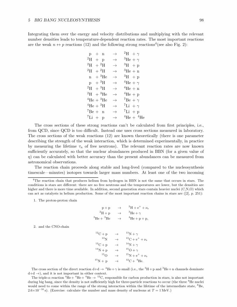
5 BIG BANG NUCLEOSYNTHESIS 98

Integrating them over the energy and velocity distributions and multiplying with the relevantnumber densities leads to temperature-dependent reaction rates. The most important reactionsare the weak n ↔ p reactions (12) and the following strong reactions4(see also Fig. 2):

p + n → 2H + γ2H + p → 3He + γ2H + 2H → 3H + p2H + 2H → 3He + n

n + 3He → 3H + p

p + 3H → 4He + γ2H + 3H → 4He + n2H + 3He → 4He + p4He + 3He → 7Be + γ4He + 3H → 7Li + γ7Be + n → 7Li + p7Li + p → 4He + 4He

The cross sections of these strong reactions can’t be calculated from first principles, i.e.,from QCD, since QCD is too difficult. Instead one uses cross sections measured in laboratory.The cross sections of the weak reactions (12) are known theoretically (there is one parameterdescribing the strength of the weak interaction, which is determined experimentally, in practiceby measuring the lifetime τn of free neutrons). The relevant reaction rates are now knownsufficiently accurately, so that the nuclear abundances produced in BBN (for a given value ofη) can be calculated with better accuracy than the present abundances can be measured fromastronomical observations.

The reaction chain proceeds along stable and long-lived (compared to the nucleosynthesistimescale—minutes) isotopes towards larger mass numbers. At least one of the two incoming

4The reaction chain that produces helium from hydrogen in BBN is not the same that occurs in stars. Theconditions is stars are different: there are no free neutrons and the temperatures are lower, but the densities arehigher and there is more time available. In addition, second generation stars contain heavier nuclei (C,N,O) whichcan act as catalysts in helium production. Some of the most important reaction chains in stars are ([2], p. 251):

1. The proton-proton chain

p + p →2H+ e+ + νe

2H+ p →3He + γ

3He + 3He →4He + p + p,

2. and the CNO-chain

12C+ p →13N+ γ

13N →13C + e+ + νe

13C+ p →14N+ γ

14N+ p →15O+ γ

15O →15N+ e+ + νe

15N+ p →12C + 4He.

The cross section of the direct reaction d+d →4He+γ is small (i.e., the 3H+p and 3He+n channels dominate

d+d →), and it is not important in either context.The triple-α reaction 4He+ 4He+ 4He → 12C, responsible for carbon production in stars, is also not important

during big bang, since the density is not sufficiently high for three-particle reactions to occur (the three 4He nucleiwould need to come within the range of the strong interaction within the lifetime of the intermediate state, 8Be,2.6×10−16 s). (Exercise: calculate the number and mass density of nucleons at T = 1MeV.)

5 BIG BANG NUCLEOSYNTHESIS 99

Figure 2: The 12 most important nuclear reactions in big bang nucleosynthesis.

nuclei must be an isotope which is abundant during nucleosynthesis, i.e., n, p, 2H or 4He. Themass numbers A = 5 and A = 8 form bottlenecks, since they have no stable or long-livedisotopes. These bottlenecks cannot be crossed with n or p. The A = 5 bottleneck is crossedwith the reactions 4He+3He and 4He+3H, which form a small number of 7Be and 7Li. Theirabundances remain so small that we can ignore the reactions (e.g., 7Be + 4He → 11C + γ and7Li + 4He → 11B+ γ) which cross the A = 8 bottleneck. Numerical calculations also show thatthe production of the other stable lithium isotope, 6Li is several orders of magnitude smallerthan that of 7Li.

Thus BBN produces the isotopes 2H, 3H, 3He, 4He, 7Li and 7Be. Of these, 3H (half life 12.3a) and 7Be (53 d) are unstable and decay after nucleosynthesis into 3He and 7Li. (7Be actuallybecomes 7Li through electron capture 7Be + e− → 7Li + νe.)

In the end BBN has produced cosmologically significant (compared to present abundances)amounts of the four isotopes, 2H, 3He, 4He and 7Li (the fifth isotope 1H= p we had already beforeBBN). Their production in the BBN can be calculated, and there is only one free parameter,

5 BIG BANG NUCLEOSYNTHESIS 100

Figure 3: The time evolution of the n, 2H (written as d) and 4He abundances during BBN. Notice howthe final 4He abundance is determined by the n abundance before nuclear reactions begin. Only a smallpart of these neutrons decay or end up in other nuclei. Before becoming 4He, all neutrons pass through2H. To improve the visibility of the deuterium curve, we have plotted it also as multiplied by a factor of50. This figure is for η = 6 × 10−10. The time at T = (90, 80, 70, 60) keV is (152, 199, 266, 367) s. Thusthe action peaks at about t = 4min. The other abundances (except p) remain so low, that to see themthe figure must be redrawn in logarithmic scale (see Fig. 4). From [3].

the baryon/photon ratio5

η ≡nB

nγ=

Ωbρcr0mNnγ0

=Ωb

mNnγ0

3H20

8πG

= 273.8 × 10−10ωb = 1.457 × 1018(

ρb0

kgm−3

)

. (22)

Here ρb0 is the average density of ordinary, or baryonic, matter today, Ωb ≡ ρb0/ρcr0 is thebaryon density parameter, and ωb ≡ Ωbh

2 .

5.7 BBN as a function of time

Let us follow nucleosynthesis as a function of time (or decreasing temperature). See Figs. 3and 4. 2H and 3H are intermediate states, through which the reactions proceed towards 4He.Therefore their abundance first rises, is highest at the time when 4He production is fastest, andthen falls as the baryonic matter ends in 4He. 3He is also an intermediate state, but the mainchannel from 3He to 4He is via 3He+n→3H+p , which is extinguished early as the free neutronsare used up. Therefore the abundance of 3He does not fall the same way as 2H and 3H. Theabundance of 7Li also rises at first and then falls via 7Li+p→4He+4He. Since 4He has a higherbinding energy per nucleon, B/A, than 7Li and 7Be have, the nucleons in them also want toreturn into 4He. This does not happen to 7Be, however, since, just like for 3He, the free neutronsneeded for the reaction 7Be+n→4He+4He have almost disappeared near the end.

5To relate η accurately to ωb we have to decide what value to use for mN . The most precise determination forωb is from the effect of baryon-photon acoustic oscillations on the CMB (Chapter 9) before photon decoupling.At that time the baryonic matter was about 75% protons and 25% helium. Proton mass is mp = 938.272MeVand helium nucleus mass divided by four (i.e., mass per nucleon) is 931.995MeV. Electrons are included in theconcept of baryonic matter, so that we have to add me = 0.511MeV for each proton, and half of this to eachnucleon in a helium nucleus. Helium atoms form earlier than hydrogen atoms, but atomic binding energies areso small that we can ignore them. This gives an average baryonic mass mN ≈ 937.068MeV per nucleon. Fusionreactions in the later universe will decrease this value somewhat, but the effect is smaller than the effect of heliumformation in BBN.

5 BIG BANG NUCLEOSYNTHESIS 101

Figure 4: Time evolution of the abundances of the light isotopes during BBN. Fromhttp://www.astro.ucla.edu/~wright/BBNS.html

5.8 Primordial abundances as a function of the baryon-to-photon ratio

Let us then consider BBN as a function of η (see Fig. 5). The larger is η, the higher is thenumber density of nucleons. The reaction rates are faster and the nucleosynthesis can proceedfurther. This mean that a smaller fraction of “intermediate nuclei”, 2H, 3H, and 7Li are leftover—the burning of nuclear matter into 4He is “cleaner”. Also the 3He production falls withincreasing η. However, 7Be production increases with η. In the figure we have plotted the finalBBN yields, so that 3He is the sum of 3He and 3H, and 7Li is the sum of 7Li and 7Be. Thecomplicated shape of the 7Li(η) curve is due to these two contributions: 1) For small η we getlots of “direct” 7Li, whereas 2) for large η there is very little “direct” 7Li left, but a lot of 7Be isproduced. In the middle, at η ∼ 3× 10−10, there is a minimum of 7Li production where neitherway is very effective.

The 4He production increases with η, since with higher density nucleosynthesis begins earlierwhen there are more neutrons left.

5.9 Comparison with observations

The abundances of the various isotopes calculated from BBN can be compared to the observedabundances of these elements. This is one of the most important tests of the big bang theory.A good agreement is obtained for η in the range η = 5.8–6.6× 10−10 . This was the best methodto estimate the amount of ordinary matter in the universe, until the advent of accurate CMBdata, first from the WMAP satellite starting in 2003 and then from the Planck satellite datastarting in 2013.6

The comparison of calculated abundances with observed abundances is complicated due tochemical evolution. The abundances produced in BBN are the primordial abundances of theseisotopes. The first stars form with this composition. In stars, further fusion reactions take placeand the composition of the star changes with time. Towards the end of its lifetime, the starejects its outer parts into interstellar space, and this processed material mixes with primordialmaterial. From this mixed material later generation stars form, and so on.

The observations of present abundances are based on spectra of interstellar clouds and stel-lar surfaces. To obtain the primordial abundances from the present abundances the effect ofchemical evolution has to be estimated. Since 2H is so fragile (its binding energy is so low), there

6Many cosmological parameters can be estimated from the CMB anisotropy, as will be discussed in CosmologyII. The Planck estimate[5] is ωb = 0.02242 ± 0.00014, or η = (6.14 ± 0.03) × 10−10.

5 BIG BANG NUCLEOSYNTHESIS 102

10-11

2 5 10-10

2 5 10-9

2 5 10-810

-10

10-9

10-8

10-7

10-6

10-5

10-4

10-3

10-2

10-1

100

4He

D/H3He/H

7Li/H

Figure 5: The primordial abundances of the light elements as a function of η. For 4He we give the massfraction, for D = 2H, 3He, and 7Li the number ratio to H = 1H, i.e., ni/nH.

5 BIG BANG NUCLEOSYNTHESIS 103

Figure 6: Determining the baryon/photon ration η by comparing BBN predictions to observations. Thewidth of the bands around the the curves represents the uncertainty in BBN prediction due to uncertaintyabout the reaction rates. The vertical extent of the yellow boxes represent the estimate of the primordialabundance from observations and the horizontal extent the resulting range in η to agree with BBN. Notethe small deuterium box. The only observational data on 3He is from our own galaxy, and since 3Heis both produced and destroyed in chemical evolution, we cannot infer the primordial abundance fromthem. From the review by Fields, Molaro, and Sarkar in [1].

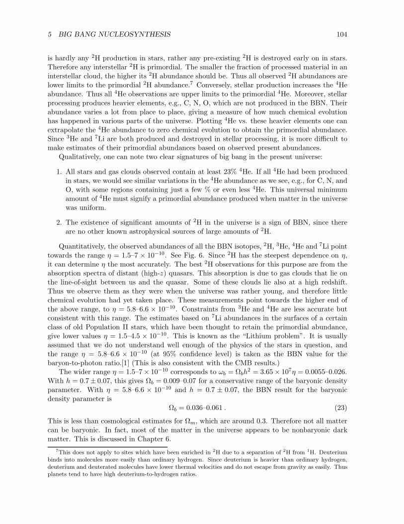
5 BIG BANG NUCLEOSYNTHESIS 104

is hardly any 2H production in stars, rather any pre-existing 2H is destroyed early on in stars.Therefore any interstellar 2H is primordial. The smaller the fraction of processed material in aninterstellar cloud, the higher its 2H abundance should be. Thus all observed 2H abundances arelower limits to the primordial 2H abundance.7 Conversely, stellar production increases the 4Heabundance. Thus all 4He observations are upper limits to the primordial 4He. Moreover, stellarprocessing produces heavier elements, e.g., C, N, O, which are not produced in the BBN. Theirabundance varies a lot from place to place, giving a measure of how much chemical evolutionhas happened in various parts of the universe. Plotting 4He vs. these heavier elements one canextrapolate the 4He abundance to zero chemical evolution to obtain the primordial abundance.Since 3He and 7Li are both produced and destroyed in stellar processing, it is more difficult tomake estimates of their primordial abundances based on observed present abundances.

Qualitatively, one can note two clear signatures of big bang in the present universe:

1. All stars and gas clouds observed contain at least 23% 4He. If all 4He had been producedin stars, we would see similar variations in the 4He abundance as we see, e.g., for C, N, andO, with some regions containing just a few % or even less 4He. This universal minimumamount of 4He must signify a primordial abundance produced when matter in the universewas uniform.

2. The existence of significant amounts of 2H in the universe is a sign of BBN, since thereare no other known astrophysical sources of large amounts of 2H.

Quantitatively, the observed abundances of all the BBN isotopes, 2H, 3He, 4He and 7Li pointtowards the range η = 1.5–7 × 10−10. See Fig. 6. Since 2H has the steepest dependence on η,it can determine η the most accurately. The best 2H observations for this purpose are from theabsorption spectra of distant (high-z) quasars. This absorption is due to gas clouds that lie onthe line-of-sight between us and the quasar. Some of these clouds lie also at a high redshift.Thus we observe them as they were when the universe was rather young, and therefore littlechemical evolution had yet taken place. These measurements point towards the higher end ofthe above range, to η = 5.8–6.6 × 10−10. Constraints from 3He and 4He are less accurate butconsistent with this range. The estimates based on 7Li abundances in the surfaces of a certainclass of old Population II stars, which have been thought to retain the primordial abundance,give lower values η = 1.5–4.5 × 10−10. This is known as the “Lithium problem”. It is usuallyassumed that we do not understand well enough of the physics of the stars in question, andthe range η = 5.8–6.6 × 10−10 (at 95% confidence level) is taken as the BBN value for thebaryon-to-photon ratio.[1] (This is also consistent with the CMB results.)

The wider range η = 1.5–7× 10−10 corresponds to ωb = Ωbh2 = 3.65× 107η = 0.0055–0.026.

With h = 0.7± 0.07, this gives Ωb = 0.009–0.07 for a conservative range of the baryonic densityparameter. With η = 5.8–6.6 × 10−10 and h = 0.7 ± 0.07, the BBN result for the baryonicdensity parameter is

Ωb = 0.036–0.061 . (23)

This is less than cosmological estimates for Ωm, which are around 0.3. Therefore not all mattercan be baryonic. In fact, most of the matter in the universe appears to be nonbaryonic darkmatter. This is discussed in Chapter 6.

7This does not apply to sites which have been enriched in 2H due to a separation of 2H from 1H. Deuteriumbinds into molecules more easily than ordinary hydrogen. Since deuterium is heavier than ordinary hydrogen,deuterium and deuterated molecules have lower thermal velocities and do not escape from gravity as easily. Thusplanets tend to have high deuterium-to-hydrogen ratios.

REFERENCES 105

5.10 BBN as a probe of the early universe

BBN is the earliest event in the history of the universe from which we have quantitative evidencein the form of numbers (primordial abundances of 2H, 3He, 4He, 7Li) that we can calculatefrom known theory and compare to observations. It can be used to constrain many kinds ofspeculations about the early universe. For example, suppose there were additional species ofparticles that were relativistic at BBN time (this is called dark radiation). This would increaseg∗ and speed up the timescale (20), leading to more primordial 4He and a higher primordialabundance of the intermediate isotopes 2H and 3He. Most such modifications of the standardpicture will ruin the agreement between theory and observations. Thus we can say that we knowwell the history of the universe since the beginning of the BBN (from T ∼ 1MeV and t ∼ 1 s),but before that there is much more room for speculation.

References

[1] Particle Data Group, Chinese Physics C 40, 100001 (2016)

[2] H. Karttunen, P. Kroger, H. Oja, M. Poutanen, and K.J. Donner: Fundamental Astronomy(Springer 1987)

[3] H. Kurki-Suonio, Nukleosynteesi isotrooppisissa ja epaisotrooppisissa kosmologioissa, Mas-ter’s thesis, University of Helsinki (1983)

[4] Planck Collaboration, Astronomy & Astrophysics 594, A13 (2016), arXiv:1502.01589

[5] Planck Collaboration, Planck 2018 results. VI. Cosmological parameters,arXiv:1807.06209v1 (2018)

6 Dark Matter

6.1 Observations

The earliest evidence for dark matter is due to Zwicky (1933). He observed (from the variationin their redshifts) that the relative velocities of galaxies in galaxy clusters were much larger thanthe escape velocity due to the mass of the cluster, if that mass was estimated from the amountof light emitted by the galaxies in the cluster. This suggested that there should actually bemuch more mass in the galaxy clusters than the luminous stars we can see. This was then calledthe “missing mass” problem. The modern terminology is to talk about dark matter, since it isunderstood that what is “missing” is not the mass, just the light from that mass.

Similar evidence comes from the rotation curves of galaxies. According to Kepler’s third law,the velocity of a body orbiting a central mass is related to its distance as

v ∝ 1

r1/2. (1)

The planets in the Solar System satisfy this relation. For the stars orbiting the center of a galaxythe situation is different, since the mass inside the orbit increases with the distance. Suppose,for example, that the mass density of a galaxy decreases as a power-law

ρ ∝ r−x (2)

with some constant x. Then the mass inside radius r is

M(r) ∝∫

r2r−xdr =r3−x

3− xfor x < 3 . (3)

Equating the acceleration of circular motion with that caused by Newtonian gravity we have

v2

r= G

M

r2∝ r1−x . (4)

Thus we find that the rotation velocity in our model galaxy should vary with distance from thecenter as

v(r) ∝ r1−x/2 . (5)

The function v(r) is called the rotation curve of a galaxy.Observed rotation curves increase with r for small r, i.e., near the center of the galaxy, but

then typically flatten out, becoming v(r) ≈ const up to as large distances as there is anythingto observe in the galaxy. From Eq. (5), this would indicate a density profile

ρ ∝ r−2 . (6)

However, the density of stars appears to fall more rapidly towards the edges of the galaxy. Also,the total mass from stars and other visible objects, like gas and dust clouds, appears to be toosmall to account for the rotation velocity at large distances. This discrepancy between visiblematter and galaxy rotation curves was established in early 1970s [1] after which this missingmass / dark matter problem became a central topic in astrophysics.

This indicates the presence of another mass component to galaxies. This mass componentshould have a different density profile than the visible, or luminous, mass in the galaxy, so thatit could be subdominant in the inner parts of the galaxy, but would become dominant in theouter parts. This dark component appears to extend well beyond the visible parts of galaxies,forming a dark halo surrounding the galaxy.

106

6 DARK MATTER 107

This can be discussed in terms of mass-to-light ratios, M/L, of various objects. It is cus-tomarily given in units of M⊙/L⊙, where M⊙ and L⊙ are the mass and absolute luminosityfor the Sun. The luminosity of a star increases with its mass faster than linearly, so that starswith M > M⊙ have M/L < 1, and smaller stars have M/L > 1. Small stars are more com-mon than large stars, so a typical mass-to-light ratio from the stellar component of galaxies isM/L ∼ a few. For stars in our part of the Milky Way galaxy, M/L ≈ 2.2. Because large starsare more short-lived, M/L increases with the age of the star system, and the typical M/L fromstars in the universe is somewhat larger. However, this still does not account for the full massesof galaxies.

The mass-to-light ratio of a galaxy turns out to be difficult to determine; the larger volumearound the galaxy you include, the largerM/L you get. But theM is determined from velocitiesof orbiting bodies and at large distances there may be no such bodies visible. For galaxy clustersyou can use the velocities of the galaxies themselves as they orbit the center of the cluster. Themass-to-light ratios of clusters appears to be several hundreds. Presumably isolated galaxieswould have similar values if we could measure them to large enough radii.

From galaxy surveys, the luminosity density of the universe is

ρL = 2.0± 0.7 × 108hL⊙ Mpc−3 . (7)

(Peacock [3], p.368; Efstathiou et al. 1988 [4]). Multiplying this with a typical mass-to-light ratiofrom galaxy clusters (Peacock, pp. 372–374),

M/L ∼ 300h–400h , (8)

we find an estimate for the density of clustered1 mass in the universe,

ρm = (M/L) · ρL ∼ 0.39–1.08 × 1011h2M⊙/Mpc3 (9)

= 2.6–7.3× 10−27h2kg/m3 . (10)

(We equate the clustered mass with matter, since gravity causes mass, but not radiation orvacuum energy, to cluster. Implicitly we are assuming that all, or most of, matter clusters formstars, so that we can observe them.) Comparing to the critical density

ρcr0 = h2 · 1.88 × 10−26kg/m3 , (11)

we get thatΩm = 0.14–0.39 . (12)

The estimates for the amount of ordinary matter in the objects we can see on the sky, starsand visible gas and dust clouds, called luminous matter, give a much smaller contribution,

Ωlum . 0.01 (13)

to the density parameter. In Chapter 5 we found that big bang nucleosynthesis leads to anestimate

Ωb = 0.036–0.061 (14)

for baryonic matter.Thus we have

Ωlum < Ωb < Ωm. (15)

1“Clustered” here does not refer to just galaxy clusters, but also to isolated galaxies, which are “clusters ofmatter”.

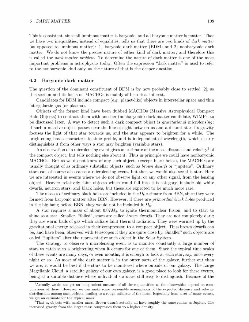
6 DARK MATTER 108

This is consistent, since all luminous matter is baryonic, and all baryonic matter is matter. Thatwe have two inequalities, instead of equalities, tells us that there are two kinds of dark matter

(as opposed to luminous matter): 1) baryonic dark matter (BDM) and 2) nonbaryonic darkmatter. We do not know the precise nature of either kind of dark matter, and therefore thisis called the dark matter problem. To determine the nature of dark matter is one of the mostimportant problems in astrophysics today. Often the expression “dark matter” is used to referto the nonbaryonic kind only, as the nature of that is the deeper question.

6.2 Baryonic dark matter

The question of the dominant constituent of BDM is by now probably close to settled [2], sothis section and its focus on MACHOs is mainly of historical interest.

Candidates for BDM include compact (e.g. planet-like) objects in interstellar space and thinintergalactic gas (or plasma).

Objects of the former kind have been dubbed MACHOs (Massive Astrophysical CompactHalo Objects) to contrast them with another (nonbaryonic) dark matter candidate, WIMPs, tobe discussed later. A way to detect such a dark compact object is gravitational microlensing :If such a massive object passes near the line of sight between us and a distant star, its gravityfocuses the light of that star towards us, and the star appears to brighten for a while. Thebrightening has a characteristic time profile, and is independent of wavelength, which clearlydistinguishes it from other ways a star may brighten (variable stars).

An observation of a microlensing event gives an estimate of the mass, distance and velocity2 ofthe compact object; but tells nothing else about it. Thus in principle we could have nonbaryonicMACHOs. But as we do not know of any such objects (except black holes), the MACHOs areusually thought of as ordinary substellar objects, such as brown dwarfs or “jupiters”. Ordinarystars can of course also cause a microlensing event, but then we would also see this star. Herewe are interested in events where we do not observe light, or any other signal, from the lensingobject. Heavier relatively faint objects which could fall into this category, include old whitedwarfs, neutron stars, and black holes, but these are expected to be much more rare.

The masses of ordinary black holes are included in the Ωb estimate from BBN, since they wereformed from baryonic matter after BBN. However, if there are primordial black holes producedin the big bang before BBN, they would not be included in Ωb.

A star requires a mass of about 0.07M⊙ to ignite thermonuclear fusion, and to start toshine as a star. Smaller, “failed”, stars are called brown dwarfs. They are not completely dark;they are warm balls of gas which radiate faint thermal radiation. They were warmed up by thegravitational energy released in their compression to a compact object. Thus brown dwarfs canbe, and have been, observed with telescopes if they are quite close by. Smaller3 such objects arecalled “jupiters” after the representative such object in the Solar System.

The strategy to observe a microlensing event is to monitor constantly a large number ofstars to catch such a brightening when it occurs for one of them. Since the typical time scalesof these events are many days, or even months, it is enough to look at each star, say, once everynight or so. As most of the dark matter is in the outer parts of the galaxy, further out thanwe are, it would be best if the stars to be monitored where outside of our galaxy. The LargeMagellanic Cloud, a satellite galaxy of our own galaxy, is a good place to look for these events,being at a suitable distance where individual stars are still easy to distinguish. Because of the

2Actually we do not get an independent measure of all three quantities, as the observables depend on com-binations of these. However, we can make some reasonable assumptions of the expected distance and velocitydistributions among such objects, leading to a rough estimate of the mass. Especially from a set of many events,we get an estimate for the typical mass.

3That is, objects with smaller mass. Brown dwarfs actually all have roughly the same radius as Jupiter. Theincreased gravity from the larger mass compresses them to a higher density.

6 DARK MATTER 109

required precise alignment of us, the MACHO, and the distant star, the microlensing events willbe rare. But if the BDM in our galaxy consisted mainly of MACHOs (with masses between thatof Jupiter and several solar masses), and we monitored constantly millions of stars in the LMC,we should observe many events every year.

Such observing campaigns (MACHO, OGLE, EROS, . . . ) were begun in the 1990s. Indeed,over a dozen microlensing events towards LMC or SMC were observed. The typical mass ofthese MACHOs turned out to by ∼ 0.5M⊙ (assuming the lenses were located in the halo of ourgalaxy), much larger than the brown dwarf mass that had been expected. The most naturalfaint object with such a mass would be a white dwarf. However, white dwarfs had been expectedto be much too rare to explain the number of observed events. On the other hand the numberof observed events is too small for these objects to dominate the mass of the BDM in the halo ofour galaxy. These mass estimates depend on the assumed distance of the lenses. If one insteadassumes that the lens is located in the same Magellanic Cloud as the star, the mass estimatesare smaller, ∼ 0.2M⊙. Then the lensing objects could be ordinary red dwarf stars, not visible tous due to this large distance. In any case, these observed lensing objects were too few to explainthe BDM of our galaxy.

The present opinion is that the BDM in our universe is dominated by thin intergalacticionized gas [2]. In fact, in large clusters of galaxies, we can see this gas, as it has been heatedby the deep gravitational well of the cluster, and radiates X-rays.

6.3 Nonbaryonic dark matter

The favorite candidates for nonbaryonic dark matter are divided into two main classes, hot darkmatter (HDM) and cold dark matter (CDM), based on the typical velocities of the particlesmaking up this matter. These particles are supposed to be at most weakly interacting, so thatthey decoupled early, or possibly they were never at thermodynamic equilibrium.

The distinction between HDM and CDM comes from their different effect on structure for-

mation in the universe. Structure formation refers to how the originally almost homogeneouslydistributed matter formed galaxies and galaxy clusters under the pull of gravity. For HDM,the velocities of the particles were large when structure formation began, making it difficultto trap them in potential wells of the forming structures. Typically these velocities were thennonrelativistic but larger than the escape velocities of the forming structures. CDM particles,on the other hand, have negligible velocities and they began to form structures early due to theirmutual gravity. Structure formation dominated by HDM leads to top-down structure formation,where the largest structures form first, and smaller structures arise from the fragmentation ofthese larger structures. Structure formation dominated by CDM leads to bottom-up structureformation, where smaller structures form first, and later they cluster or coalesce to form largerstructures. The intermediate case is called warm dark matter (WDM).

We shall discuss structure formation in Cosmology II. But we mention already that theobserved large-scale structure in the universe, i.e., how galaxies are distributed in space, andrelating it to the observed anisotropy of the CMB, which shows the primordial inhomogeneity,from which this structure grew, gives today the best way to estimate the relative amounts ofBDM, HDM, and CDM in the universe. The result is that dark matter must be dominated byCDM (or possibly it could be somewhat “warm”).

A popular class of nonbaryonic dark matter are thermal relics, particles and antiparticlesthat were initially in thermodynamic equilibrium, but decoupled early enough to prevent theirannihilation with each other at least to some extent. For thermal relics there is another cleardistinction between HDM and CDM: HDM particles decoupled while they were relativistic (theprime example is the neutrinos). They have therefore retained a large number density, and thustheir masses must be small, less than 100 eV, for their total mass density not to exceed the

6 DARK MATTER 110

estimated dark matter density. Today, the HDM particles should be nonrelativistic—otherwisewe would not classify them as “matter”. CDM particles decouple while nonrelativistic and thusa much smaller relic number density is left over. Thus CDM particles must typically be heavyfor CDM to form a significant part of dark matter. Since after decoupling the thermal relicCDM temperature falls as a−2, CDM is extremely cold when structure formation begins.

However, there is another possibility for CDM: particles that were never in thermal equi-librium; these can have small velocities and still a large relic number density, requiring theirmasses to be small (the main such candidate is called the axion).

6.4 Hot dark matter

The main candidate for HDM are neutrinos with a small but nonzero rest mass. The cosmicneutrino background would make a significant contribution to the density parameter if theneutrinos had a rest mass of the order of 1 eV.

For massive neutrinos, the number density today is the same as for massless neutrinos, buttheir energy density today is dominated by their rest masses, giving (factor 3

4from their fermionic

nature · factor 411

from their lower temperature after electron-positron annihilation = 311)

ρν =

3∑

ν=1

mνnν =3

11nγ

∑

mν . (16)

For T0 = 2.725K, this gives for the neutrino density parameter

Ωνh2 =

∑

mν

94.14 eV, (17)

which applies if the neutrino masses are well below the neutrino decoupling temperature, ∼1MeV, but well above the present temperature of massless neutrinos, Tν0 = 0.168meV. Thiscounts then as one contribution to Ωm. As discussed in Chapter 4, neutrino oscillation measure-ments constrain

∑

mν within the range 0.06–6 eV, so that Ων = 0.001–0.16.If neutrinos dominated the masses of galaxies there would be a lower limit to their mass

called the Tremaine–Gunn limit due to the available phase space inside the galaxy volume andbelow the galaxy escape velocity. This is because neutrinos are fermions and the Pauli exclusionprinciple prevents two neutrinos from occupying the same quantum state. A similar limit wouldapply to any fermion candidates for the dominant component of dark matter, but not to bosons.

Exercise: Tremaine–Gunn limit. Suppose neutrinos dominate the mass of galaxies (i.e., ignoreother forms of matter). We know the mass of a galaxy (within a certain radius) from its rotation velocity.The mass could come from a smaller number of heavier neutrinos or a larger number of lighter neutrinos,but the available phase space (you don’t have to assume a thermal distribution) limits the total numberof neutrinos, whose velocity is below the escape velocity. This leads to a lower limit on the neutrino massmν . Let r be the radius of the galaxy, and v its rotation velocity at this distance. Find the minimum mν

needed for neutrinos to dominate the galaxy mass, assuming all three species have the same mass. (Arough estimate is enough: you can, e.g., assume that the neutrino distribution is spherically symmetric,and that the escape velocity within radius r equals the escape velocity at r). Give the numerical valuefor the case v = 220 km/s and r = 10kpc. Repeat the calculation assuming that only one of the three νspecies is massive. (We know today that neutrinos are only a small part of dark matter, but a similarlimit applies to any fermions.)

Data on large scale structure and CMB combined with structure formation theory requiresthat a majority of the matter in the universe has to be CDM (or possibly WDM) and the presentupper limit to HDM (massive neutrinos) is [5]

ων ≡ Ωνh2 . 0.0025 (18)

6 DARK MATTER 111

requiring that the sum of the three neutrino masses satisfies

∑

mν . 230meV . (19)

Thus neutrinos make only a small contribution to dark matter,

0.0007 . Ωνh2 . 0.0025 , (20)

where the lower limit comes from the∑

mν ≥ 0.06 from neutrino oscillations.

6.5 Cold dark matter

Observations require that dark matter is dominated by CDM. No known particle is suitable toact as CDM; therefore this conclusion implies that the standard model of particle physics mustbe extended with additional particles.

A major class of CDM particle candidates is called WIMPs (Weakly Interacting MassiveParticles). We mentioned already that because of the large number density of neutrinos, theirmasses must be small, in order not to “close the universe” with an energy density > ρcr. How-ever, if the mass of some hypothetical weakly interacting particle species is much larger than thedecoupling temperature of weak interactions, these particles will be largely annihilated beforethis decoupling, leading to a much lower number density, so that again it becomes possible toachieve a total density < ρcr starting from an initial thermal distribution at very high temper-atures. (We calculate this in the next section.) Thus the universe may contain two classes ofweakly interacting particles, very light (the neutrinos) and very heavy (the WIMPs), with acosmologically interesting density parameter value.

The favorite kind of WIMP is provided by the supersymmetric partners of known particles,more specifically, the “lightest supersymmetric partner” (LSP), which could be a stable weaklyinteracting particle. It should have a mass of the order of 100GeV. It has been hoped that,if it exists, it could be created and detected at CERN’s LHC (Large Hadron Collider) particleaccelerator. A measurement of its properties would allow a calculation of its expected numberand energy density in the universe. So far (2018) there has been no detection, already considereda disappointment.

A candidate CDM particle should thus be quite heavy, if it was in thermal equilibriumsometime in the early universe. One CDM candidate, the axion, is, however, very light; butit was “born cold” and has never been in thermal interaction. It is related to the so-called“strong CP-problem” in particle physics. We shall not go into the details of this, but it can bephrased as the question “why is the neutron electric dipole moment so small?”. It is zero to theaccuracy of measurement, the upper limit being dn < 0.30 × 10−25ecm (Particle Data Group2016 [6]), whereas it has a significant magnetic dipole moment. A proposed solution involves anadditional symmetry of particle physics (the Peccei–Quinn symmetry). The axion would thenbe the “Goldstone boson of the breaking of this symmetry”. The important point for us is thatthese axions would be created in the early universe when the temperature fell below the QCDenergy scale (of the order of 100MeV), and they would be created “cold”, i.e., with negligiblekinetic energy, and they would never be in thermal interaction. Thus the axions have negligiblevelocities, and act like CDM.

If these WIMPs or axions make up the CDM, they should be everywhere, also in the SolarSystem, although they would be very difficult to detect. A direct detection is not impossible,however. Sensitive detectors have been built with this purpose. WIMPs and axions require arather different detection technology.

One kind of an axion detector is a low noise microwave cavity in a strong magnetic field. Anaxion may interact with the magnetic field and produce a microwave photon. No axions have

6 DARK MATTER 112

so far been detected. On the other hand the detectors have so far not been sensitive enough forus to really expect a detection.

WIMPs interact weakly with ordinary matter. In practice this means that mostly they donot interact at all, so that a WIMP will pass through the Earth easily, without noticing it, butoccasionally, very rarely, there will be an interaction. A typical interaction is elastic scatteringfrom a nucleus, with an energy exchange of a few keV.4 A very sensitive WIMP detector candetect if this much energy is deposited on its target material. The problem is that there aremany other “background” events which may cause a similar signal. Thus these WIMP detectorsare continuously detecting something.

Therefore the experimentalists are looking for an annual modulation in the signal they ob-serve. The WIMPs should have a particular velocity distribution related to the gravitationalwell of our galaxy. The Earth is moving with respect to this velocity distribution, and theannual change in the direction of Earth’s motion should result in a corresponding variation inthe detection rate. One such experiment, DAMA,5 has already claimed that they detect suchan annual variation in the signal they observe, signifying that some of the events they see aredue to WIMPs. Other experiments have not been able to confirm this detection.

6.6 Decoupling

An important class of dark matter particle candidates are thermal relics, particles that wereonce in thermal equilibrium and survived because they decoupled before they were annihilated.

Decoupling is the process where a particle species makes a transition from a high interactionrate with other particles to a low, and eventually negligible, interaction rate. While the interac-tion rate is high, the interactions keep the particles in thermal equilibrium with other species.When the interaction rate becomes low enough the particles decouple from other species. Ifthe decoupled particles are stable (or have very long lifetime, i.e., negligible decay rate), theirnumber will then stay constant so that their number density falls with the expansion as n ∝ a−3.

Consider the case where the main interaction of particle species x with other species (y, z)is particle-antiparticle annihilation and creation:

x + x ↔ y + z . (21)

For simplicity, assume an equal number of particles an antiparticles, nx = nx, i.e., that µx = 0.(If µx 6= 0 but just very small, we can check after the calculation whether this was a goodapproximation, i.e., if the thermal relic density we get with the µx = 0 approximation is largecompared to the particle-antiparticle excess. If µx is important, i.e., particles survive mainlybecause there were more particles than antiparticles, we wouldn’t usually call them thermalrelics.) The x particle number density nx then evolves according to

dnxdt

+ 3Hnx = −〈σv〉nxnx + ψ , (22)

where σ is the annihilation cross section (the effective area the other particle presents as atarget), v is the relative velocity of the colliding particles, 〈·〉 indicates the mean value takenover the particle momentum space distribution, and ψ is the rate of creation of x particles.

In equilibrium, as many particles are created as annihilated. Thus

ψ = 〈σv〉n2eq , (23)

4Note that weak interactions are “weak” in the sense that they occur rarely, but the energy exchange in suchan interaction, when it occurs, does not have to be very small.

5http://www.lngs.infn.it/en/dama

6 DARK MATTER 113

where neq is the equilibrium value of nx and nx, and we can rewrite (22) as

dnxdt

+ 3Hnx = −〈σv〉(

n2x − n2eq)

. (24)

The Hubble parameter H gives the time scale at which external conditions, and thus also neq,change. Define

Γ ≡ neq〈σv〉 , (25)

the reaction rate per particle in equilibrium (τ ≡ 1/Γ gives the mean time between interactionsfor an x particle). We have to compare Γ to H to determine whether the interaction rate is highor low. Defining the comoving number density

Nx ≡ nxa3 and Neq ≡ neqa

3 (26)

we can rewrite (24) as

1

Neq

dNx

d ln a= − Γ

H

[

(

Nx

Neq

)2

− 1

]

. (27)

(It is often practical to use the logarithm of the scale factor ln a as time coordinate. It changesby one when the universe expands by a factor e.)

If Γ ≫ H (τ ≪ H−1), the interactions keep Nx very close to Neq, since a small deviation isenough to make the rhs of (27) large and cause a rapid corrective change in Nx. On the otherhand, if Γ ≪ H (τ ≫ H−1), the rhs stays negligible no matter how much Nx deviates from Neq

and thus Nx stays constant. Typically a particle species is in the Γ ≫ H regime at first, butmay make a transition to the Γ ≪ H regime (decouple) later. We call the temperature Td atwhich Γ = H, the decoupling temperature. (Decoupling is also called “freeze-out”.)

The constant comoving number density after decoupling is the comoving relic density of theparticles. A crude approximation (the instantaneous decoupling approximation) is

Nx(relic) ≈ Nx(Td) ≈ Neq(Td) , (28)

which we get if we assume that Nx follows Neq until T = Td, and stays constant after that.There are two distinct situations: 1) Hot thermal relics: particles that were ultrarelativistic

(Td > mx) when they decoupled. Their relic density is large, ∼ T 3. 2) Cold thermal relics:particles that were nonrelativistic (Td ≪ mx) when they decoupled. Thus most of them annihi-lated after T fell below mx, but decoupling saved the rest. Thus cold thermal relics survive inmuch smaller numbers than hot thermal relics. We already discussed neutrinos, which are hotthermal relics, in Chapter 4. Let us now consider cold thermal relics.

Cold thermal relics decouple while they are nonrelativistic, so that their equilibrium numberdensity then is

neq(Td) = gx

(

mTd2π

)3/2

e−m/Td , (29)

where m is the mass of the relic particle. After decoupling nx ∝ a−3, so that the present (relic)density is

nx0 ≈ g∗S(T0)

g∗S(Td)

(

T0Td

)3

neq(Td) . (30)

The problem is to find Td, the decoupling temperature where Γd ≡ neq(Td)〈σv〉 = H.The annihilation cross section σ depends on the particle and associated theory, but on

general quantum theoretical grounds σv can be expanded in terms of velocity squared, withcontributions σv ∝ v2q, where q = 0 is called s-wave annihilation, q = 1 p-wave annihilation etc.For the nonrelativistic case, v ≪ 1, the s-wave annihilation is dominant, unless prohibited for

6 DARK MATTER 114

some reason in which case the p-wave is dominant. For an equilibrium distribution, the meanspeed of a nonrelativistic particle is 〈v〉 =

√

8/π√

T/m. Since v ∝ (T/m)1/2, we can write

〈σv〉 = σ0

(

T

m

)q

, where q = 0 (for s) or q = 1 (for p) . (31)

Thus

Γd = σ0

(

Tdm

)q

neq(Td) = σ0gx

(2π)3/2m3y−q−3/2e−y , (32)

wherey ≡ m

Td≫ 1 . (33)

In the early universe, the relation between the Hubble parameter and temperature is

H2 =8πG

3

π2

30g∗(T )T

4 (34)

so that

Hd =

√

g∗(Td)

90

πm2

MPl

y−2 (35)

where MPl ≡ 1/√8πG = 2.436 × 1018 GeV is the reduced Planck mass. The decoupling tem-

perature can be solved from the equation

Γd

Hd= Ay1/2−qe−y = 1 , (36)

where

A ≡√

45

4π5g∗(Td)gxMPlmσ0 . (37)

Given gx, m, σ0, q, and an initial guess for g∗(Td), we can solve Td numerically from (36).The relic number density is, from (30) and (29),

nx0 ≈ g∗S(T0)

g∗S(Td)

(

T0Td

)3

gx

(

mTd2π

)3/2

e−y

=gx

(2π)3/2g∗S(T0)

g∗S(Td)y3/2e−yT 3

0

=gx

(2π)3/2g∗S(T0)

g∗S(Td)A−1y1+qT 3

0

=

√

g∗(Td)

90

g∗S(T0)

g∗S(Td)

π

MPlmσ0y1+qT 3

0 , (38)

where we used e−y = A−1yq−1/2 from (36) to get rid of the exponential dependence on y (thisallows us to use an approximate value for y below). We get the relic mass (energy) density bymultiplying with m,

ρx0 =

√

g∗(Td)

90

g∗S(T0)

g∗S(Td)

π

MPlσ0y1+qT 3

0 . (39)

Relating nx0 to the present CMB photon number density nγ0 = (2ζ(3)/π2)T 30 , we have

nx0nγ0

=π3

ζ(3)

√

g∗(Td)

360

g∗S(T0)

g∗S(Td)

y1+q

MPlmσ0. (40)

6 DARK MATTER 115

Assuming that decoupling happens before electron-positron annihilation and that no particlespecies is becoming nonrelativistic during the decoupling, we can set g∗(Td) = g∗S(Td), andusing the numerical value g∗S(T0) ≈ 3.938, this becomes

nx0nγ0

=π3

ζ(3)

1√360

g∗S(T0)√

g∗(Td)

y1+q

MPlmσ0≈ 5.35

y1+q

√

g∗(Td)MPlmσ0. (41)

For an analytical estimate of y, we can solve Eq. (36) iteratively: Taking the logarithm, itbecomes

y = lnA+ (12− q) ln y . (42)

For y ≫ 1, ln y is a slowly varying function of y, allowing for rapidly convergent iteration. Wemake our first guess for y by ignoring the term with ln y:

y0 = lnA (43)

and then iteratey1 = lnA+ (1

2− q) ln y0 . (44)

For our rough estimate this first iteration is enough, and we take

y ≈ y1 = lnA+ (12− q) ln(lnA) . (45)

where A ∝ mσ0, so that y depends logarithmically on m and σ0.The relic density depends mainly on m and σ0. Assuming a fixed σ0, we see that the relic

number density decreases with increasing m, so that the cold thermal relic mass density ρx0depends only logarithmically on the relic particle mass m. However, as we see in the nextsection, σ0 may depend on m, changing these conclusions.

6.7 WIMP miracle

Consider now a hypothetical particle with a mass in the GeV range, gx = 2 (spin-12fermion),

s-wave annihilation (q = 0) with a typical weak interaction cross section

σ0 ∼ G2FE

2 ∼ G2Fm

2 (46)

where GF = 1.17 × 10−5 GeV−2 is the Fermi constant.We have then MPlmσ0 ≈ 3.3 × 108(m/GeV)3. Since now σ0 ∝ m2 and mσ0 ∝ m3, we see

that the relic densities depend on the mass as

nx0 ∝1

m3and ρx0 ∝

1

m2(47)

(besides the logarithmic dependence via y). Thus the cold thermal relic mass density decreaseswith increasing relic particle mass, whereas for hot thermal relics, the number density is inde-pendent of m and the mass density increases proportional to m.

The decoupling temperature Td = m/y depends only logarithmically on g∗(Td), so the precisevalue of g∗(Td) is not important. If we assume that decoupling happened between the electroweakand QCD transitions, g∗(Td) is between 60 and 100 (in the standard model). Taking g∗(Td) = 60,we get that A ≈ 1.63 × 107(m/GeV)3 and lnA ≈ 16.6 + 3 ln(m/GeV). The value of y is closeto this.

For example, for m = 3 GeV, lnA = 19.9 and y ≈ lnA + 12ln(lnA) ≈ 21.4, so that Td =

m/y ≈ 0.14 GeV. With a higher mass, we get a higher decoupling temperature. For m =100 GeV, lnA = 30.4, y = 32.1, and Td = 3.1 GeV.

6 DARK MATTER 116

For the relic number density we get (approximating further y ≈ lnA)

nx0nγ0

≈ 5.35y

√

g∗(Td)MPlmσ0= 2.1 × 10−9y

( m

GeV

)−3

≈ 3.5× 10−8(

1 + 0.18 lnm

GeV

)( m

GeV

)−3

. (48)

Taking the baryon-to-photon ratio to be η = 6×10−10, we get for the ratio of cold thermal relicsto baryons

nx0nB0

≈ 58(

1 + 0.18 lnm

GeV

)( m

GeV

)−3

, (49)

and since mN ≈ 1 GeV the mass density ratio

ρx0ρb0

≈ 58(

1 + 0.18 lnm

GeV

)( m

GeV

)−2

. (50)

Since ρb0 ≈ 0.05ρcr0, the requirement that such relic particles (with energy density ρx0 + ρx0 =2ρx0) do not close the universe gives the lower bound m & 2.6 GeV for their mass (the Lee-

Weinberg bound). The corresponding upper bound for a massive neutrino species (a hot thermalrelic) was mν . 50 eV (from Eq. (17) with h ∼ 0.7).

We get the observed CDM to baryon density ratio ρc0/ρb0 ≈ 5.3 [5] for m ≈ 5.3 GeV.6 Thefact that we get the right dark matter density for a cold thermal relic with a weak interactioncross section and mass roughly corresponding to the electroweak scale7, is called the WIMP

miracle. Such particles appear naturally in extensions to the standard model of particle physics,like supersymmetry (SUSY), which predicts SUSY partners to standard model particles, so thismakes them a very natural candidate for dark matter. Such dark matter candidates are calledWIMPs (weakly interacting massive particles).

In the minimal supersymmetric extension to the standard model (MSSM) such a particlewith a mass of a few GeV would already have been discovered in particle colliders. The lowermass limit for fermionic SUSY partners in MSSM is 15GeV [7]. Ongoing experiments at LHCare pushing this limit up. With a typical weak interaction σ0 such heavier WIMPs would makejust a small contribution to the dark matter. As the relic density is inversely proportional toσ0 (besides the logarithmic dependence via y) we can save WIMPs as the main CDM candidateif we assume a smaller interaction cross section. There is enough freedom to adjust parametersin extensions to the standard model that this is possible. Such parameters are constrained byboth collider and direct detection experiments.

6.8 Dark Matter vs. Modified Gravity

Since all the evidence for non-standard-model dark matter comes so far from its gravitationaleffects, it has been suggested that it does not exist, and instead the law of gravity needs to bemodified over large distances. While actual proposals for such gravity modifications (MOND,TeVeS) do not appear very convincing and lead to difficulties of their own, it certainly would becomforting to have a direct laboratory detection of a CDM particle.

Evidence for the standard view of dark matter comes from collisions of clusters of galaxies[8],see Fig. 1. According to this standard view the mass of a cluster of galaxies has three maincomponents: 1) the visible galaxies, 2) the intergalactic gas, and 3) cold dark matter. The lastcomponent should have the largest mass, and the first one the smallest. When two clusters ofgalaxies collide, it is unlikely for individual galaxies to collide, since most of the volume, and

6Note that ρc denotes the CDM energy density and ρcr the critical density.7The electroweak scale is more like 100GeV, but this is considered close enough.

6 DARK MATTER 117

Figure 1: This is a composite image of galaxy cluster 1E 0657-56, also called the Bullet Cluster. Itconsists of two subclusters, a larger one on the left, and a smaller one on the right. They have recentlycollided and traveled through each other. One component of the image is an optical image which showsthe visible galaxies. Superposed on it, in red, is an X-ray image, which shows the heated intergalacticgas, that has been slowed down by the collision and left behind the galaxy components of the clusters.The blue color is another superposed image, which represent an estimate of the total mass distributionof the cluster, based on gravitational lensing. NASA Astronomy Picture of the Day 2006 August 24.Composite Credit: X-Ray: NASA/CXC/CfA/M. Markevitch et al. Lensing map: NASA/STScI; ESOWFI; Magellan/U. Arizona/D. Clowe et al. Optical: NASA/STScI; Magellan/U. Arizona/D. Clowe etal.

REFERENCES 118

cross section, in a cluster is intergalactic space. The intergalactic gas is too thin to slow downthe relatively compact galaxies noticeably. On the other hand, the intergalactic gas componentsdo not travel through each other freely but are slowed down by the collision and heated up. Thusafter the clusters have traveled through each other, much of the intergalactic gas is left behindbetween the receding clusters. Cold dark matter, in turn, should be very weakly interacting,and thus practically collisionless. Thus the CDM components of both clusters should also travelthrough each other unimpeded.

Figure 1 is a composite image of such a collision of two clusters. We see that the intergalacticgas has been left behind the galaxies in the collision. The mass distribution of the system hasbeen estimated from the gravitational lensing effect on the apparent shapes of galaxies behindthe cluster. If there were no cold dark matter, most of the mass would be in the intergalactic gas,whose mass is estimated to be about five times that of the visible galaxies. Even in a modifiedgravity theory, we would expect most of the lensing effect to be where most of the mass is, eventhough the total mass estimate would be different. However, the image shows that most of themass is where the galaxies are. This agrees with the cold dark matter hypothesis, since colddark matter should move like the galaxies in the collision.

References

[1] K.C. Freeman, Astrophys. J. 160, 811, Appendix A (1970); M.S. Roberts, A.H. Rots, As-tronomy & Astrophysics 26, 483 (1973); J.P. Ostriker, P.J.E. Peebles, A. Yahil, Astrophys.J. Lett. 193, L1 (1974); J. Einasto, A. Kaasik, E. Saar, Nature 250, 309 (1974); V.C.Rubin, W.K. Ford Jr, N. Thonnard, Astrophys. J. Lett. 225, L107 (1978)

[2] F. Nicastro et al., Observations of the missing baryons in the warm-hot intergalactic

medium, Nature 558, 406 (2018)

[3] J.A. Peacock, Cosmological Physics, Cambridge University Press 1999

[4] G. Eftstahiou, R.S. Ellis, B.A. Petersin, MNRAS 232, 431 (1988)

[5] Planck Collaboration, Astronomy & Astrophysics 594, A13 (2016), arXiv:1502.01589

[6] Particle Data Group, Chinese Physics C 40, 100001 (2016)

[7] G. Belanger et al., arXiv:1308.3735, Physics Letters B 726, 773 (2013)

[8] D. Clowe et al., astro-ph/0608407, Astrophys. J. Lett. 648, L109 (2006)

A More about General Relativity

A.1 Vectors, tensors, and the volume element

The metric of spacetime can always be written as

ds2 = gµνdxµdxν ≡

3∑

µ=0

3∑

ν=0

gµνdxµdxν . (1)

We introduce Einstein’s summation rule: there is a sum over repeated indices (that is, we don’tbother to write down the summation sign

∑

in this case). Greek (spacetime) indices go overthe values 0–3, Latin (space) indices over the values 1–3, i.e., gijdx

idxj ≡∑

3

i=1

∑

3

j=1gijdx

idxj .The objects gµν are the components of the metric tensor. They have, in principle, the dimensionof distance squared. In practice one often assigns the dimension of distance (or time) to somecoordinates, and then the corresponding components of the metric tensor are dimensionless.These coordinate distances are then converted to proper (“real” or “physical”) distances withthe metric tensor. The components of the metric tensor form a symmetric 4× 4 matrix.

Example 1. The metric tensor for a 2-sphere (discussed in Chapter 2 as an example of acurved 2D space) has the components

[gij ] =

[

a2 00 a2 sin2 ϑ

]

. (2)

Example 2. The metric tensor for Minkowski space has the components

gµν =

−1 0 0 00 1 0 00 0 1 00 0 0 1

(3)

in Cartesian coordinates, and

gµν =

−1 0 0 00 1 0 00 0 r2 00 0 0 r2 sin2 ϑ

(4)

in spherical coordinates.Example 3. The Robertson-Walker metric, which we discuss in Chapter 3, has components

gµν =

−1 0 0 0

0 a2

1−Kr20 0

0 0 a2r2 00 0 0 a2r2 sin2 ϑ

. (5)

Note that the metric tensor components in the above examples always formed a diagonalmatrix. This is the case when the coordinate system is orthogonal.

The vectors which occur naturally in relativity are four-vectors, with four components, e.g.,the four-velocity. The values of the components depend on the basis eα used. Note that theindex of the basis vector does not refer to a component, but specifies which one of the fourbasis vectors is in question. The components of the basis vectors in the basis they define are, ofcourse,

(eα)β = δβα , (6)

119

A MORE ABOUT GENERAL RELATIVITY 120

where δβα is the Kronecker symbol, 1 if α = β, 0 otherwise.Given a coordinate system, we have two bases (also called frames) naturally associated with

it, the coordinate basis and the corresponding normalized basis. If the coordinate system isorthogonal, the latter is an orthonormal basis. When we use the coordinates to define thecomponents of a vector, like the 4-velocity in Chapter 2, the components naturally come outin the coordinate basis. The basis vectors of a coordinate basis are parallel to coordinate lines,and their length represents the distance from changing the value of the coordinate by one unit.For example, if we move along the coordinate x1 so that it changes by dx1, the distance traveledis ds =

√

g11dx1dx1 =√g11dx

1. The length of the basis vector e1 is thus√g11. Since in

the coordinate basis the basis vectors usually are not unit vectors, the numerical values of thecomponents give the wrong impression of the magnitude of the vector. Therefore we may wantto convert them to the normalized basis

eα ≡( 1√

|gαα|)

eα . (7)

(It is customary to denote the normalized basis with a hat over the index, when both bases areused. In the above equation there is no sum over the index α, since it appears only once on theleft.) For a four-vector w we have

w = wαeα = wαeα , (8)

wherewα ≡

√

|gαα|wα . (9)

For example, the components of the coordinate velocity of a massive body, vi = dxi/dt couldbe greater than one; the “physical velocity”, i.e., the velocity measured by an observer who isat rest in the comoving coordinate system, is 1

vi =√giidx

i/√

|g00|dx0 , (10)

with components always smaller than one.The volume of a region of space (given by some range in the spatial coordinates x1, x2, x3)

is given by

V =

∫

V

dV =

∫

V

√

det[gij ]dx1dx2dx3 , (11)

where dV ≡√

det[gij ]dx1dx2dx3 is the volume element. Here det[gij ] is the determinant of the

3× 3 submatrix of the metric tensor components corresponding to the spatial coordinates. Foran orthogonal coordinate system, the volume element is

dV =√g11dx

1√g22dx

2√g33dx

3. (12)

The metric tensor is used for taking scalar (dot) products of four-vectors,

w · u ≡ gαβuαwβ . (13)

The (squared) norm of a four-vector w is

w ·w ≡ gαβwαwβ. (14)

Exercise: Show that the norm of the four-velocity is always −1.

1When g00 = −1, this simplifies to√giidx

i/dt.

A MORE ABOUT GENERAL RELATIVITY 121

For an orthonormal basis we have

e0· e

0= −1

e0· ej = 0

ei · ej = δij . (15)

We shall use the short-hand notation

eα · eβ= ηαβ , (16)

where the symbol ηαβ is like the Kronecker symbol δαβ, except that η00 = −1.

A.2 Contravariant and covariant components

We sometimes write the index as a subscript, sometimes as a superscript. This has a precisemeaning in relativity. The component wα of a four-vector is called a contravariant component.We define the corresponding covariant component as

wα ≡ gαβwβ . (17)

The norm is now simplyw ·w = wαw

α. (18)

In particular, for the 4-velocity we always have

uµuµ = gµνu

µuν =ds2

dτ2= −1 . (19)

We defined the metric tensor through its covariant components (Eq. 1). We now define thecorresponding covariant components gαβ as the inverse matrix of the matrix [gαβ ],

gαβgβγ = δγα . (20)

Nowgαβwβ = gαβgβγw

γ = δαγwγ = wα. (21)

The metric tensor can be used to lower and raise indices. For tensors,

A βα = gαγA

γβ

Aαβ = gαγgβδAγδ

Aαβ = gαγgβδAγδ. (22)

Note that for the mixed components A βα 6= Aβ

α, unless the tensor is symmetric, in which casewe can write Aβ

α. When indices form covariant-contravariant pairs and are summed over, as inAαβγB

αβγ the resulting quantity is invariant in coordinate transformations.For an orthonormal basis,

gαβ

= gαβ = ηαβ , (23)

and the covariant and contravariant components of vectors and tensors have the same values,except that the raising or lowering of the time index 0 changes the sign. These orthonormalcomponents are also called “physical” components, since they have the “right” magnitude.

Note that the symbols δαβ and ηαβ are not tensors, and the location of their index carriesno meaning.

A MORE ABOUT GENERAL RELATIVITY 122

A.3 Einstein equation

From the first and second partial derivatives of the metric tensor,

∂gµν/∂xσ, ∂2gµν/(∂x

σ∂xτ ) , (24)

one can form various curvature tensors. These are the Riemann tensor Rµνρσ, the Ricci tensor

Rµν ≡ Rαµαν , and the Einstein tensor Gµν = Rµν − 1

2gµνR, where R is the Ricci scalar gαβRβα,

also called the “scalar curvature” (not to be confused with the scale factor of the Robertson–Walker metric, which is sometimes denoted R(t)). We shall not discuss these curvature tensorsin this course. The only purpose of mentioning them here is to be able to show the generalform of the Einstein equation, before we go to the much simpler specific case of the Friedmann–Robertson–Walker universe.

In Newton’s theory the source of gravity is mass, or, in the case of continuous matter, themass density ρ. According to Newton, the gravitational field gN is given by the equation

∇2Φ = −∇ · gN = 4πGρ . (25)

Here Φ is the gravitational potential.In Einstein’s theory, the source of spacetime curvature is the energy-momentum tensor, also

called the stress-energy tensor, or, for short, the “energy tensor” T µν . The energy tensor carriesthe information on energy density, momentum density, pressure, and stress. The energy tensorof frictionless continuous matter (a perfect fluid) is

T µν = (ρ+ p)uµuν + pgµν , (26)

where ρ is the energy density and p is the pressure in the rest frame of the fluid. In cosmology wecan usually assume that the energy tensor has the perfect fluid form. T 00 is the energy densityin the coordinate frame. (T i0 gives the momentum density, which is equal to the energy fluxT 0i. T ij gives the flux of momentum i-component in j-direction.)

We can now give the general form of the Einstein equation,

Gµν = 8πGT µν . (27)

This is the law of gravity according to Einstein. Comparing to Newton (Eq. 25) we see that themass density ρ has been replaced by T µν , and∇2Φ has been replaced by the Einstein tensor Gµν ,which is a short way of writing a complicated expression containing first and second derivativesof gµν . Thus the gravitational potential is replaced by the 10 components of gµν in Einstein’stheory.

In the case of a weak gravitational field, the metric is close to the Minkowski metric, and wecan write, e.g.,

g00 = −1− 2Φ (28)

(in suitable coordinates), where Φ is small. The Einstein equation for g00 becomes then

∇2Φ = 4πG(ρ+ 3p) . (29)

Comparing this to Eq. (25) we see that the density ρ has been replaced by ρ+3p. For relativisticmatter, where p can be of the same order of magnitude than ρ this is an important modificationto the law of gravity. For nonrelativistic matter, where the particle velocities are v ≪ 1, wehave p ≪ ρ, and we get Newton’s equation.

When applied to a homogeneous and isotropic universe filled with ordinary matter, theEinstein equation tells us that the universe cannot be static, it must either expand or contract.2

2Equation (44) leads to a < 0, which does not allow a(t) = const . If we momentarily had a = 0, a wouldimmediately begin to decrease.

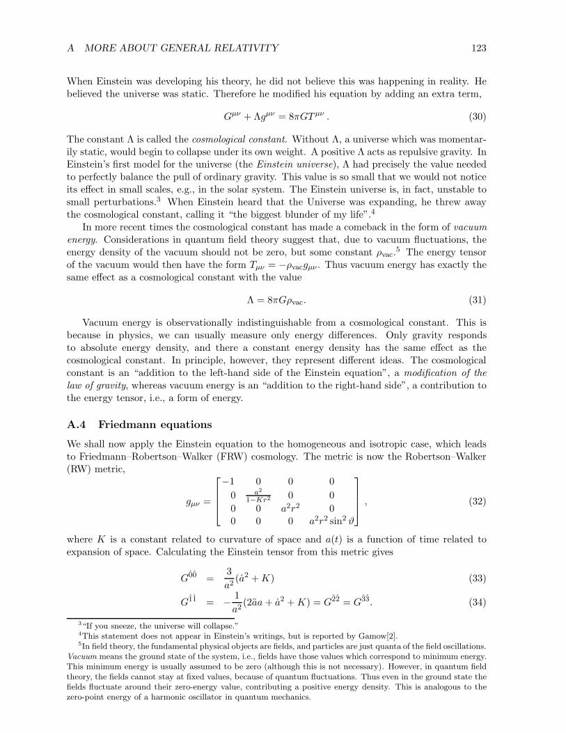
A MORE ABOUT GENERAL RELATIVITY 123

When Einstein was developing his theory, he did not believe this was happening in reality. Hebelieved the universe was static. Therefore he modified his equation by adding an extra term,

Gµν + Λgµν = 8πGT µν . (30)

The constant Λ is called the cosmological constant. Without Λ, a universe which was momentar-ily static, would begin to collapse under its own weight. A positive Λ acts as repulsive gravity. InEinstein’s first model for the universe (the Einstein universe), Λ had precisely the value neededto perfectly balance the pull of ordinary gravity. This value is so small that we would not noticeits effect in small scales, e.g., in the solar system. The Einstein universe is, in fact, unstable tosmall perturbations.3 When Einstein heard that the Universe was expanding, he threw awaythe cosmological constant, calling it “the biggest blunder of my life”.4

In more recent times the cosmological constant has made a comeback in the form of vacuumenergy. Considerations in quantum field theory suggest that, due to vacuum fluctuations, theenergy density of the vacuum should not be zero, but some constant ρvac.

5 The energy tensorof the vacuum would then have the form Tµν = −ρvacgµν . Thus vacuum energy has exactly thesame effect as a cosmological constant with the value

Λ = 8πGρvac. (31)

Vacuum energy is observationally indistinguishable from a cosmological constant. This isbecause in physics, we can usually measure only energy differences. Only gravity respondsto absolute energy density, and there a constant energy density has the same effect as thecosmological constant. In principle, however, they represent different ideas. The cosmologicalconstant is an “addition to the left-hand side of the Einstein equation”, a modification of the

law of gravity, whereas vacuum energy is an “addition to the right-hand side”, a contribution tothe energy tensor, i.e., a form of energy.

A.4 Friedmann equations

We shall now apply the Einstein equation to the homogeneous and isotropic case, which leadsto Friedmann–Robertson–Walker (FRW) cosmology. The metric is now the Robertson–Walker(RW) metric,

gµν =

−1 0 0 0

0 a2

1−Kr20 0

0 0 a2r2 00 0 0 a2r2 sin2 ϑ

, (32)

where K is a constant related to curvature of space and a(t) is a function of time related toexpansion of space. Calculating the Einstein tensor from this metric gives

G00 =3

a2(a2 +K) (33)

G11 = − 1

a2(2aa+ a2 +K) = G22 = G33. (34)

3“If you sneeze, the universe will collapse.”4This statement does not appear in Einstein’s writings, but is reported by Gamow[2].5In field theory, the fundamental physical objects are fields, and particles are just quanta of the field oscillations.

Vacuum means the ground state of the system, i.e., fields have those values which correspond to minimum energy.This minimum energy is usually assumed to be zero (although this is not necessary). However, in quantum fieldtheory, the fields cannot stay at fixed values, because of quantum fluctuations. Thus even in the ground state thefields fluctuate around their zero-energy value, contributing a positive energy density. This is analogous to thezero-point energy of a harmonic oscillator in quantum mechanics.

REFERENCES 124

We use here the orthonormal basis (signified by theˆover the index).We assume the perfect fluid form for the energy tensor

T µν = (ρ+ p)uµuν + pgµν . (35)

Isotropy implies that the fluid is at rest in the RW coordinates, so that uµ = (1, 0, 0, 0) and(remember, gµν = ηµν = diag(−1, 1, 1, 1))

T µν =

ρ 0 0 00 p 0 00 0 p 00 0 0 p

. (36)

Homogeneity implies that ρ = ρ(t), p = p(t).The Einstein equation Gµν = 8πGT µν becomes now

3

a2(a2 +K) = 8πGρ (37)

−2a

a−

(

a

a

)2

− K

a2= 8πGp . (38)

Let us rearrange this pair of equations to6

(

a

a

)2

+K

a2=

8πG

3ρ (43)

a

a= −4πG

3(ρ+ 3p) . (44)

These are the Friedmann equations. (“Friedmann equation” in singular refers to Eq. 43.)

References

[1] C.W. Misner, K.S. Thorne, J.A. Wheeler, Gravitation (Freeman 1973)

[2] G. Gamow, My Worldline (Viking Press 1970), p. 44, cited onhttps://blogs.scientificamerican.com/guest-blog/einsteins-greatest-blunder/

6Including the cosmological constant Λ these equations take the form

3

a2(a2 +K)− Λ = 8πGρ (39)

−2a

a−

(

a

a

)2

−K

a2+ Λ = 8πGp . (40)

or, in the rearranged form,

(

a

a

)2

+K

a2−

Λ

3=

8πG

3ρ (41)

a

a−

Λ

3= −

4πG

3(ρ+ 3p) . (42)

We shall not include Λ in these equations. Instead, we allow for the presence of vacuum energy ρvac, which hasthe same effect.

C Numerical Constants

C.1 Defining constants

The following constants of nature are used to define SI units and therefore they have exactnumerical values in them 1. The second equalities define the natural units we use in this course.

c = 299 792 458m/s = 1 defines meter

h = 6.626 070 15 × 10−34 Js = 2π defines kilogram

kB = 1.380 649 × 10−23 J/K = 1 defines kelvin

e = 1.602 176 634 × 10−19 C defines ampere (1)

C.2 Other constants of nature

G = 6.674 30 ± 15× 10−11 m3/kgs2

mPl = 1.220 890 ± 14× 1019 GeV (2)

C.3 Mathematical constants

Approximate values:

π ≈ 3.14159 26535 8979

e ≈ 2.71828 18284

ζ(3) ≈ 1.20205 69032

(3)

C.4 Astronomical units

Julian year ≡ 365.25 days = 31 557 600 s

light year = 9 460 730 472 580 800m (exact)

AU = 149 597 870 700m (2012 definition)

pc ≡ 3600 (180/π)AU ≈ 206 264.806 247AU

≈ 3.085 677 581 49 × 1016 m ≈ 3.261 564 light years (4)

C.5 Cosmological quantities

Present CMB temperature [1]

T0 = 2.7255 ± 0.0006K

⇒ nγ0 =2ζ(3)

π2T 3

0 ≈ 410.73 photons/cm3

ργ0 = 2π2

30T 4

0 ≈ 4.6451 × 10−31 kg/m3 (5)

1physics.nist.gov/cuu/Units/current.html

125

REFERENCES 126

References

[1] D.J. Fixsen, The Temperature of the Cosmic Microwave Background, Astrophys. J. 707,916 (2009)