Cost- and Price Dynamics of Solar PV Modules

Stefan Reichelstein∗

Graduate School of Business

Stanford University

and

Anshuman Sahoo

Steyer-Taylor Center for Energy Policy and Finance

Stanford University

November 2015

∗Contact information: reichelstein@stanford.edu; asahoo@stanford.edu

We gratefully acknowledge financial support from the Steyer-Taylor Center for Energy Policy and Finance

and a U.S. Department of Energy (DOE) grant administered through the Bay Area Photovoltaics Consortium

(BAPVC). We thank seminar participants at Stanford, New York University, Southern Methodist University

and the Antitrust Division of the U.S. Department of Justice for their helpful comments and suggestions.

We also acknowledge the assistance of Aneesh Raghunandan with our data collection.

Cost- and Price Dynamics of Solar PV Modules

November 2015

Abstract: This paper develops a model framework and a corresponding empirical inference

procedure for estimating long-run marginal cost in industries where production costs decline

over time. In the context of the solar photovoltaic module industry, we rely on firm-level

financial accounting data to estimate the long-run marginal cost of PV modules for the

years 2008 -2013. During those years, the industry experienced both sharp price declines

and significant expansions of manufacturing capacity. By comparing the trajectory of average

sales prices with the long-run marginal cost estimates, we are in a position to quantify the

extent to which actual price declines were attributable to excess capacity as opposed to

reductions in production costs. While we find a significant effect attributable to excess

capacity for some quarters in our sample period, the dynamics of this industry also points to

a rate of cost reductions that is even faster than the 80% learning curve which has described

the trajectory of average sales prices over the past three decades.

Keywords: Long-run marginal cost, Cost estimation, Learning-by-doing, Price dynamics

JEL codes: D41, L11, L63, M21, Q42

1 Introduction

Economic theory argues that in a competitive industry the equilibrium price for a homoge-

neous product will be equal to the long-run marginal cost of production. Yet, the identifica-

tion and measurement of marginal cost remains a matter of debate in industrial organization,

in particular when costs are expected to decline over time.1 This paper proposes and im-

plements a method for estimating long-run marginal cost based on firm-level data obtained

from financial statements. The resulting trajectory of cost estimates can be compared to

actually observed sales prices, with the resulting difference serving as a measure of the extent

of disequilibrium at different points in time. Furthermore, the observed time series of cost

estimates can be extrapolated to forecast future cost- and price reductions.

We apply our framework in the context of the solar photovoltaic (PV) module industry.

In recent years, this industry has experienced sharp price declines for solar PV modules

and rapid growth in the volume of output. Figure 1 plots the history of (the logarithm) of

average sales prices against (the logarithm of) cumulative output for the years 1979 to 2010.

The corresponding price trajectory conforms closely to an 80% constant elasticity learning

curve, a finding that is frequently attributed to Swanson (2011).2 Accordingly, prices drop

by 20% with every doubling of cumulative output, measured in megawatts (MW).

Figure 1: Plot from Swanson (2011)

1See, for instance, the discussion in Carlton and Perloff (2005), Pittman (2009) and Rogerson (2011)

about the inclusion and representation of capital assets in the measurement of long-run marginal cost.2Figure 1 shows that for the years 2008-2009, ASPs were distinctly above the trend line suggested by

the 80% learning curve. Most industry observers attribute this discrepancy to an acute polysilicon shortage

which temporarily increased the raw material cost of silicon wafers.

1

Figure 2 extends the original Swanson plot beyond 2010 and shows that between 2011

and 2013 the decline in average sales prices (ASP) for PV modules was substantially steeper

than that predicted by the historical 80% learning curve. Particularly noteworthy is the

40% price drop in 2011 alone and the rebound in prices for late 2013. Industry analysts

have pointed out that the steep price declines in recent years may reflect at least in part

that the additions to industry-wide manufacturing capacity were excessive. Recent studies,

like Candelise, Winskel, and Gross (2013), have pointed out the difficulty in attributing the

dynamics of observed sales prices to intrinsic cost reductions as opposed to broader industry

level effects.3

Figure 2: Predicted and observed ASPs, 2008 – 2013. All prices are in 2013 U.S. dollars.

The front part of our analysis formulates a dynamic model of a competitive industry

in which firms make a sequence of overlapping capacity investments and then choose their

subsequent output levels in a competitive fashion, taking market prices as given.4 While the

long-run marginal cost contains components that are sunk in the short-run, the expected

market prices will in equilibrium nonetheless be equal to the long-run marginal cost, because

firms are capacity constrained in the short run. Furthermore, firms will earn zero economic

3In particular, Candelise, Winskel, and Gross (2013) state:“Overall, it is not straightforward to fully

disentangle module price reductions due to reduced production costs related to device and production process

improvements and economies of scale along the PV module chain from market demand/supply dynamics,

including manufacturers strategies....” (page 100).4Similar models of overlapping capacity investments have been considered in Arrow (1964), Rogerson

(2008), Rajan and Reichelstein (2009), and Nezlobin (2012) in connection with managerial performance

evaluation and profitability analysis.

2

profits on their capacity investments if the expected market prices in future periods are equal

to the long-run marginal cost in those future periods.5 Accordingly, we refer to the long-run

marginal cost at a particular point in time as the Economically Sustainable Price (ESP).

In most manufacturing industries, including solar PV modules, the long-run marginal

cost comprises capacity related costs for machinery and equipment, current manufacturing

costs for materials, labor and overhead as well as periodic costs related to selling and admin-

istrative expenses. Our formulation allows for the possibility that both the cost of capacity

and periodic operating costs decrease over time due to exogenous technological progress and

learning-by-doing effects. For the firms in our sample, we infer production costs from quar-

terly financial statements, primarily based on cost of goods sold, finished goods inventory

balances and general and administrative expenses. In addition, our cost inference procedure

relies on quarterly data for manufacturing capacity and product shipments, as reported by

firms in the industry and analysts.

In applying our cost estimation procedure to solar PV modules, we obtain a close match

between average sales prices and economically sustainable prices for the years 2008 - 2010.6

Beginning in late 2011, however, we conclude that the dramatic decline in the observed

ASPs for most of the years 2012-2013 is not consistent with the industry having been in

equilibrium.7 In other words, for those time periods the drop in ASPs should in significant

part be attributed to excessive additions to manufacturing capacity rather than to cost

reductions. Furthermore, the difference between the ASP’s and estimated ESPs indicates

the price effect that we attribute to excess capacity in the industry at different points in

time.

Despite our conclusion that excessive capacity additions drove observed sales prices below

the long-run marginal cost for some of the quarters in our observation window, our econo-

metric results also point to a rate of cost reductions that is even faster than suggested by the

5The link between full cost, including in particular capacity related costs, and product pricing has been

studied in the managerial accounting literature; see, for instance, Banker and Hughes (1994), Gox (2002),

Balakrishnan and Sivaramakrishnan (2002), Narayanan (2003) and Reichelstein and Rohlfing-Bastian (2015).

Most of these studies consider a firm with monopoly pricing power and identify the optimal mark-up for

setting product prices above some appropriate measure of cost.6The solar PV industry satisfies the criteria of a competitive industry insofar as a large number of firms

in the industry supply a relatively homogeneous product. To note, the median market share of firms in this

industry was less than 1% in 2012.7This conclusion is corroborated by the sharply negative earnings and declining share prices that firms

in the industry experienced during those two years.

3

80% learning curve. In particular, for core manufacturing costs, which comprise materials,

labor, and manufacturing overhead, our estimates point to a 74% constant elasticity learning

curve. At the same time, we find that capacity related costs for machinery and equipment

have fallen at a rate that also outperforms the 80% learning rate benchmark. Taken to-

gether, these results yield a forecast for the trajectory of future long-run marginal cost, and

therefore also for future module prices, that is steeper than the traditional learning curve

associated with this industry.

The research design of our analysis is applicable beyond the solar PV industry. Since

the empirical inference procedure outlined in this paper is based on firm-level accounting

data, any long-run marginal cost estimate will, ceteris paribus, become more reliable if the

product or service in question is (i) fairly homogeneous across suppliers and (ii) constitutes

the dominant line of business for firms in the sample. From that perspective, semiconductors,

chemicals, aircraft manufacturing and steel would be other natural candidates.8 In industries

where firms typically deliver a heterogeneous mix of products and/or services, one would

need to conduct the empirical tests either for product aggregates or obtain access to line-of

-business segment reports.9

Our results are directly related to several recent studies on the cost structure of solar PV

modules. The analysis by Pillai and McLaughlin (2013) is closet in spirit to our work, as these

authors study the mark-up that firms can charge over and above cost of goods sold (COGS).

In particular, their analysis seeks to predict the sensitivity of mark-ups to changes in the price

of polysilicon, a key raw material in the production of modules. On a per unit sold basis,

COGS reflects the accountant’s measure of full production cost. This cost is always lower

than the economically sustainable price.10 The approach in Pillai and McLaughlin (2013) is

consistent with our notion of equilibrium insofar as firms would need to charge a mark-up

on COGS in order to arrive at a product price that covers the economically sustainable

price. Given a homogeneous product, our model setting would furthermore predict higher

8For semiconductors and chemicals, the earlier work of Lieberman (1984) and Dick (1991) has demon-

strated significant cost reductions due to technological progress and learning-by-doing.9For instance, our approach could potentially be implemented for a segment of comparable product retail-

ers if the entire range of their store keeping units is aggregated into a single product category “merchandise”.10In the context of a static investment model, Reichelstein and Rohlfing-Bastian (2015) demonstrate

formally that the long-run marginal cost exceeds full cost, as commonly measured in accounting. The main

reasons are that (i) full cost (COGS) does not include general and administrative expenses and (ii) capacity

related costs are not fully reflected in the depreciation charges that are included in COGS.

4

mark-ups for low cost producers.

The cost inference method we employ to estimate the ESP complements so-called “bottom-

up” cost models, e.g., Powell et al. (2012), Powell et al. (2013), Goodrich et al. (2013a), and

Goodrich et al. (2013b). These studies estimate costs by aggregating input requirements

and input prices as reported by various industry sources. Our estimation approach, based

on firm-level accounting information, yields several estimates related to core manufacturing-

and capacity costs that broadly confirm those obtained from bottom-up cost models. In

contrast to our approach, though, these models provide a snapshot of different costs at par-

ticular point in time, rather than a dynamic cost model in which equilibrium prices are based

on anticipated future cost reductions.

Recent work by Pillai (2015) has identified several explanatory variables for the decrease

in COGS among module manufacturers from 2005 to 2012: (i) a reduction in input polysil-

icon prices, (ii) a shift in production to China, (iii) technological innovations, including

a lower polysilicon utilization rate and higher module efficiencies, and (iv) lower capacity

costs associated with larger capacity orders. While our findings document cost reductions

for certain cost categories, Pillai’s analysis provides additional insight by identifying actual

”drivers” of learning such as polysilicon usage rates and improved efficiency of the solar cells.

Consistent with Pillai (2015), our regression analysis also seeks to separate out the impact

that lower capacity costs and lower polysilicon prices have on learning rates.

The remainder of the paper is organized as follows. Section 2 formulates a dynamic model

of a competitive industry with falling production costs and formally derives the concept of

an Economically Sustainable Prices (ESP). Section 3 describes our inferential procedure for

deriving the ESP from firm-level accounting data. We then compare our ESP estimates to

observed ASPs. Section 4 presents our econometric estimates of recent learning effects in

manufacturing costs and applies these estimates to extrapolate a trajectory of future ESPs.

Section 5 concludes. The Appendix presents proofs, data sources and adjustments as well

as robustness checks.

5

2 A Model of Economically Sustainable Prices

2.1 Base Model

The model framework developed in this section allows us to identify economically sustainable

prices in terms of production costs. We consider a dynamic model of an industry composed

of a large number of suppliers who behave competitively. A key feature of the model is

that firms are capacity constrained in the short-run. Each firm’s output supplied to the

market in a particular period is limited to the overall capacity that the firm has installed in

previous periods. Production capacity available at any given point in time therefore reflects

the cumulative effect of past investments.

In the base version of the model, firms can accurately predict future demand. Let P ot (Qt)

denote the aggregate willingness-to-pay (inverse demand) curve at time t, where Qt denotes

the aggregate quantity supplied at date t. Market demand is assumed to be decreasing in

price and, in addition, we postulate that demand is expanding over time in the sense that:

P ot+1(Q) ≥ P o

t (Q), (1)

for all t ≥ 1 and all Q. The significance of this condition is that if firms make investments

sufficient to meet demand in the short-run, they will not find themselves with excess capacity

in future periods.11 This condition appears plausible in the context of solar PV modules,

particularly for the time period covered in our empirical analysis.

In order to break even on their capacity investments, firms must realize a stream of

revenues that cover periodic operating costs in addition to investment expenditures. The

economically sustainable price is cost-based and comprises capacity related costs, periodic

operating costs, and costs related to income tax payments. At the initial date 0, the industry

is assumed to have a certain stock of capacity in place. To acquire one unit of manufacturing

capacity, i.e., the capacity to manufacture annually a solar PV module capable of generating

one Watt (W) of power, firms must incur an investment expenditure of v at the initial date

0. We allow for technological progress resulting in lower capacity acquisition costs over

time. For reasons of tractability, though, we confine attention to a single “technological

progress parameter”, η, leading to a pattern of geometric declines such that ηt · v denotes

11Rogerson (2008) and Rogerson (2011) refer to (1) as the No-Excess Capacity (NEC) condition. See also

Rajan and Reichelstein (2009) and Dutta and Reichelstein (2010).

6

the acquisition cost for one unit of capacity at time t, with η ≤ 1.12 Accordingly, investment

decisions and the subsequent level of aggregate capacity in the market are conditional on

firms’ expectation of future decreases in capacity costs.

Investments in capacity represent a joint cost insofar as one unit of capacity acquired at

time t will allow the firm to produce one unit of output in each of the next T periods.13 To

identify equilibrium prices in terms of costs, it will be useful to introduce the marginal cost

of one unit of capacity made available for one period of time. As shown by Arrow (1964) and

Rogerson (2008), this effectively amounts to “levelizing” the initial investment expenditure.

To that end, let γ = 11+r

denote the applicable discount factor. The marginal cost of one

unit of capacity in period t then becomes:

ct =ηt · v

T∑τ=1

(γ · η)τ. (2)

An intuitive way to verify this claim is to assume that firms in the industry can rent

capacity services on a periodic basis. Assuming this rental market is competitive and capacity

providers have the same cost of capital, it is readily verified that the capacity provider who

invests in one unit of capacity at time t and then rents out that capacity in each of the next

T periods for a price of ct+τ would exactly break even on his initial investment of ηt · v.

Accordingly, Arrow (1964) refers to ct as the user cost of capacity.

In any given period, firms are assumed to incur fixed operating costs, e.g., maintenance,

rent, and insurance, in proportion to their capacity. Like past investment expenditures, these

costs are assumed to be effectively “sunk” after date t because they are incurred regardless

of capacity utilization. Formally, let ft represent the fixed operating cost per unit of capacity

available at time t, with ft+1 ≤ ft for all t ≥ 1. Finally, production of one unit of output

entails a constant unit variable cost, wt, which again is assumed to be weakly decreasing

over time, that is, wt+1 ≤ wt for all t ≥ 1. In contrast to the fixed operating costs, variable

costs are avoidable in the short-run if the firm decides not to utilize its available capacity.

12Decreases in capacity cost as a function of time can be attributed to improvements in manufacturing

equipment.13For simplicity, we adopt the assumption that productive capacity remains constant over the useful life

of a facility. In the regulation literature, this productivity pattern is frequently referred to as the ”one-hoss

shay” model; see, for instance, Rogerson (2008) and Nezlobin, Rajan, and Reichelstein (2012).

7

Corporate income taxes affect the long-run marginal cost of production through depre-

ciation tax shields and debt tax shields, as both interest payments on debt and depreciation

charges reduce the firm’s taxable income. Following the standard corporate finance approach,

we ignore the debt related tax shield provided the applicable discount rate, r, is interpreted

as a weighted average cost of capital. The depreciation tax shield is determined by both

the effective corporate income tax rate and the allowable depreciation schedule for the facil-

ity. The effective corporate income tax rate is represented as α (in %), and dt denotes the

percentage of the initial asset value that is the allowable tax depreciation charge in year t,

1 ≤ t ≤ T .

The assumed useful life of an asset for tax purposes is usually shorter than the asset’s

actual economic useful life, which we denote by T in our model. Accordingly, we set dt = 0

for those periods that exceed the useful life of the asset for tax purposes. As shown below,

the impact of income taxes on the long-run marginal cost can be summarized by a tax factor

which amounts to a “mark-up” on the unit cost of capacity, ct.

∆ =

1− α ·T∑t=1

dt · γt

1− α. (3)

To provide intuition for the expression in (3), we note that corporate income taxes would

not affect the economically sustainable price if taxable income were calculated on cash flow

basis. In that (hypothetical) case, both the present value of pre-tax cash flows and taxable

incomes would be equal to zero if the product price is equal to the economically sustainable

price. Thus firms would break even both on a pre-tax basis and after taxes. Accordingly, ∆

would be equal to 1 if the tax code were to allow for immediate full expensing of investments

and therefore taxable income would be equal to pre-tax cash flow. However, since the tax

code only allows for a delayed write-off of the capital expenditure, corporate income taxes

will generally introduce an additional cost factor.14

We are now in a position to formally introduce our concept of the economically sustainable

price in terms of the different production cost components:

14Specifically, ∆ = 1 if d0 = 1 and dt = 0 for t ≥ 1. Holding α constant, a more accelerated tax schedule

tends to lower ∆ closer to one. To calibrate the magnitude of this factor, for a corporate income tax rate of

35%, and a tax depreciation schedule corresponding to a 150% declining balance rule over 20 years, the tax

factor would approximately amount to ∆ = 1.3.

8

ESPt = wt + ft + ct ·∆. (4)

Given our assumption of a competitive fringe of suppliers, the investment and capac-

ity levels of individual firms remain indeterminate. Denoting the aggregate industry-wide

investment levels by It, the “one-hoss shay” assumption that productive assets have undi-

minished productivity for T periods implies that the aggregate capacity at date t is given

by:

Kt = It−T + It−T+1 + . . .+ It−1. (5)

Equation (5) holds only for t > T . If t ≤ T , then Kt = I0 + I1 + ...+ It−1.

Firms choose their actual output in a manner that is consistent with competitive supply

behavior. Since capacity related costs and fixed operating costs are sunk in any given period,

firms will exhaust their entire capacity only if the market price covers at least the short-

run marginal cost wt. Conversely, firms would rather idle part of their capacity with the

consequence that the market price will not drop below wt. Given an aggregate capacity level,

Kt, in period t, the resulting market price is therefore given by:

pt(Kt, wt) = max{wt, P ot (Kt)},

while the aggregate output level, Qt(Kt, wt) satisfies P ot (Qt(Kt, wt)) = pt(Kt, wt). We refer

to the resulting output and price levels as competitive supply behavior.

Definition 1 {K∗t }∞t=1 is an equilibrium capacity trajectory if, given competitive supply be-

havior, capacity investments have a net present value of zero at each point in time.

Finding 1 The trajectory given by:

ESPt = P ot (K∗t ) (6)

is an equilibrium capacity trajectory.15

The equilibrium price characterization in Finding 1 supports our interpretation of the

ESPt as the long-run marginal cost of one unit of output. Firms’ capacity investments are

15A formal proof of Finding 1 is presented in Appendix A. An implicit assumption here is that the

aggregate capacity in place at the initial date does not amount to excess capacity. Formally, we require

P ot (K0) > ESP1.

9

assumed to be forward looking as they anticipate future cost reductions. With additional

assumptions, the capacity trajectory identified in Finding 1 is also the unique equilibrium

capacity trajectory. This is readily seen if one assumes that capacity investments are re-

versible or, instead, that capacity can be obtained on a rental basis for one period at a time,

with all rental capacity providers obtaining zero economic profits. Competition would then

force the market price for the product in question to be equal to ESPt in each period.16

In our model formulation, the unit variable costs, wt, and the unit fixed cost, ft, may

decline over time, with the rate of decline taken as exogenous. We note that under conditions

of atomistic competition, that is, no firm can impact the prevailing market price through its

own supply decision, the result in Finding 1 also extends to situations where the unit costs

decline as a function of the cumulative volume of past output levels. One possible formulation

is for wt = β(∑Qt) ·w, where β(·) ≤ 1 is decreasing in its argument and

∑Qt ≡

∑τ≤tQτ .

17

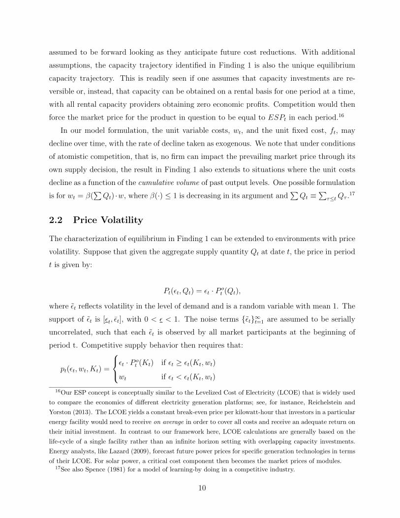
2.2 Price Volatility

The characterization of equilibrium in Finding 1 can be extended to environments with price

volatility. Suppose that given the aggregate supply quantity Qt at date t, the price in period

t is given by:

Pt(εt, Qt) = εt · P ot (Qt),

where εt reflects volatility in the level of demand and is a random variable with mean 1. The

support of εt is [εt, εt], with 0 < ε < 1. The noise terms {εt}∞t=1 are assumed to be serially

uncorrelated, such that each εt is observed by all market participants at the beginning of

period t. Competitive supply behavior then requires that:

pt(εt, wt, Kt) =

εt · P ot (Kt) if εt ≥ εt(Kt, wt)

wt if εt < εt(Kt, wt)

16Our ESP concept is conceptually similar to the Levelized Cost of Electricity (LCOE) that is widely used

to compare the economics of different electricity generation platforms; see, for instance, Reichelstein and

Yorston (2013). The LCOE yields a constant break-even price per kilowatt-hour that investors in a particular

energy facility would need to receive on average in order to cover all costs and receive an adequate return on

their initial investment. In contrast to our framework here, LCOE calculations are generally based on the

life-cycle of a single facility rather than an infinite horizon setting with overlapping capacity investments.

Energy analysts, like Lazard (2009), forecast future power prices for specific generation technologies in terms

of their LCOE. For solar power, a critical cost component then becomes the market prices of modules.17See also Spence (1981) for a model of learning-by doing in a competitive industry.

10

where the threshold level of demand volatility is given by:

εt(Kt, wt) =

εt if εt · P o

t (Kt) ≤ wt

wt

P ot (Kt)

if εt · P ot (Kt) > wt > εt · P o

t (Kt)

εt if εt · P ot (Kt) ≥ wt.

Given Kt and wt, the expected market price in period t then becomes:

E [pt(wt, εt, Kt)] ≡∫ ε(Kt,wt)

ε

wt · ht(εt) dεt +

∫ ε

ε(Kt,wt)

ε · P ot (Kt) · ht(εt) dεt. (7)

With risk neutral firms, price volatility will not affect the capacity levels obtained in

equilibrium provided firms anticipate that they will exhaust the available capacity even for

unfavorable price shocks. To that end, we introduce a condition of limited price volatility :

εt · ESPt ≥ wt.

Holding the distributions ht(·) of εt fixed, this condition will be satisfied if the short-run

avoidable cost wt constitutes a relatively small percentage of the long-run marginal cost,

ESPt. The implication of this condition is that even for unfavorable price fluctuations firms

will still want to deploy their entire capacity.

Corollary to Finding 1 If price volatility is limited, the trajectory identified in Finding 1

remains an equilibrium capacity trajectory. The expected market prices in equilibrium satisfy:

ESPt = E [pt(wt, εt, K∗t )] . (8)

As will become clear in the empirical part below, the limited price volatility condition

appears plausible in the context of the solar PV module industry for the years 2008-2013.

Our estimates suggest that the unit variable cost, wt, accounts for less than 65% of the total

ESPt. The limited price volatility condition will therefore hold provided εt ≥ 0.65. To be

sure, some firms may have idled part of their available capacity during those years, but this

observation could be attributed to the industry having been out of equilibrium, at least in

parts of 2012 and 2013, rather than to more significant unfavorable price shocks.

If the above condition of limited price volatility does not hold, the expected equilibrium

price will still be equal to the ESP in period t under additional conditions. Reichelstein and

11

Rohlfing-Bastian (2015) establish this result in a finite horizon model in which firms make a

single investment at the initial date and then supply output in a sequentially optimal manner

given current market conditions. In equilibrium, the aggregate capacity level will generally

be higher than that emerging under limited price volatility if firms anticipate that with some

probability the aggregate capacity of the industry will not be exhausted. The intuition for

this result is that since market prices are bounded below by the short-run variable cost,

significant price volatility essentially entails a call option in the firm’s payoff structure.18 In

order for the zero-profit condition to hold, the aggregate capacity level must, ceteris paribus,

therefore increase.

In the context of our infinite horizon setting with overlapping capacity investments,

a natural candidate for an equilibrium, regardless of the degree of price volatility, is the

sequence {Kot }∞t=1 implicitly defined by the equations:

ESPt = E [pt(wt, εt, Kot )] . (9)

Clearly, Kot = K∗t if price volatility is limited. The sequence {Ko

t }∞t=1 will indeed be an

equilibrium capacity trajectory, regardless of whether volatility is limited or not, provided

the corresponding capacity levels increase (weakly) over time, i.e., Kot+1 ≥ Ko

t , so that

in equilibrium the industry will always seek to expand the aggregate capacity level.19 A

sufficient condition, in turn, for the Kot to increase monotonically is that φt+1(K) > φt(K)

for any K, where φt(K) ≡ E [pt(wt, εt, K)].

3 Estimating Economically Sustainable Prices

This section presents our method for estimating the long-run marginal cost of production,

based on firm-level financial accounting data supplemented by data obtained from an indus-

try analyst (Lux Research). Our model framework has conceptualized the long-run marginal

cost in each period as the sum of capacity related costs and current operating costs. Since

we estimate these cost components primarily from income statements, our approach needs

18Similarly, Baldenius, Nezlobin, and Vaysman (2015) examine a model of managerial performance eval-

uation in which the optimal investment policy is such that in response to negative shocks firms will leave

parts of their capacity idle in some periods.19Of course, this constraint is of no importance if one postulates a competitive fringe of contract man-

ufacturers that effectively provide a rental market for manufacturing capacity, as assumed in parts of the

investment literature; see, for instance, Abel and Eberly (2011).

12

to follow the basic accounting distinction between manufacturing (inventoriable) costs and

period costs. The former pertain to factory-related costs, including materials, labor and man-

ufacturing overhead, including depreciation. These inventoriable costs are reported either as

part of cost of goods sold (COGS) or as additions to inventory on the balance sheet.20 In

contrast, period costs cover selling as well as general and administrative (SG&A) expenses,

including advertising and R&D. Conceptually, we think of wt and ft from Section 2 as having

two components each: wt = w+t + w−t and ft = f+

t + f−t , with the “+” part referring to

manufacturing (inventoriable) costs and the “-” part referring to period costs.

Table 1 lists the variables we rely on as part of our estimation procedure. We use the

time index, t ∈ {1, ..., 24}, to refer to individual quarters. Following industry convention,

module output is measured by the overall power generated, in terms of Watts (W) delivered

by the module.21

All of the variables in Table 1 are obtained from firms’ financial statements, except for

the last three: sit, Kit, and Iit,. These three variables were obtained either from quarterly

or annual reports by the firms in our sample, or from press releases. Lux Research (2012a)

provides a default source in the absence of data disclosed by the companies themselves. As

shown in the next subsection, the first three variables, qit, nit, and COGMit, in Table 1 are

inferred from the remaining variables, rather than observed directly.

The major steps of the solar PV value chain include the sequential production of polysil-

icon, ingots, wafers, cells, and modules. Polysilicon is used to grow ingots, and these are

subsequently sliced into wafers. Wafers are then processed to create cells, which convert

light energy into electricity. In the final step, cells are strung and bound together into a

solar PV module. Further details about the individual manufacturing steps are provided by

Lux Research (2012b) and in the online Appendix.22

Our sample includes ten major module manufacturers with a combined market share of

35%. Since these firms are listed on U.S. stock exchanges, their financial statements have

been prepared in accordance with U.S. GAAP rules. The firms in our sample are Yingli

20Some firms in our sample sell products other than solar modules which introduces some noise in our

COGS measure. However, these other products account for a small share of the firms’ revenues. To illustrate,

between 2008 and 2012, 96.5% to 98.7% of Yingli’s revenues were from sales of modules. In 2013, ReneSola’s

annual report splits sales data only according to modules and wafers.21For numerical convenience, quarterly output is usually stated in terms of megawatts (MW). We also

follow the industry practice that all Watt measures are stated in terms of direct current (DC).22The Online Appendix is available at http://stanford.io/1ov1kdQ.

13

Variable Description Units

qit Production volume MW

nit Inventory volume MW

COGMit Cost of goods manufactured $

Salesit Module sales $

COGSit Cost of goods sold $

GMit Gross margin $

Dit Depreciation charge $

Invit Inventory value $

CAPXit Capital expenditures $

RDit Research and development expense $

SGAit Selling, general, and administrative expenses $

ASPit Average sales price $/W

sit Sales volume MW

Kit Production capacity MW/year

Iit Addition to production capacity MW/year

Table 1: Variables used in ESP estimation.

Green Energy, Trina Solar, Suntech Power, Canadian Solar, LDK Solar, Hanwha SolarOne,

JA Solar, ReneSolar, Jinko Solar, and China Sunergy.23 Almost 300 other firms supply the

solar PV module market (Lux Research, 2012a), though we excluded manufacturers based

on four criteria: (i) lower than 0.5% share of global capacity in 2012, (ii) privately held or

embedded within large conglomerates, (iii) listed on exchanges outside of the U.S, and (iv)

relying on thin-film rather than crystalline silicon technology.24 Our data span 24 quarters

from Q1 2008 to Q4 2013, yielding a sample of 214 cost observations.

23We access financial data through the Bloomberg terminal system. Table 6 in Appendix B provides

summary details about the firms. The U.S. based firm SunPower is not in our sample because its sizeable

solar development business makes it difficult to infer manufacturing costs from reported financial information.24The firms in our sample are quite similar in terms of of the efficiency of their solar cells. In contrast,

Pillai and McLaughlin (2013) note significant variation in cell efficiency for their sample and therefore make

corresponding efficiency adjustments.

14

3.1 Manufacturing Costs

3.1.1 Core Manufacturing Costs

We use the label core manufacturing costs to refer to all manufacturing (inventoriable)

costs other than depreciation. The data available allow us to make inferences only about

the aggregate core manufacturing costs in period t, though not their fixed and variable

components. Thus, we seek to estimate the unit core manufacturing cost of firm i in quarter

t:

mit ≡ w+it + f+

it .

While we are not in a position to disaggregate core manufacturing costs into their variable

and fixed components, bottom-up cost estimates suggest that the variable cost percentage

accounts for 95% of the core manufacturing costs (Powell et al., 2013).25 Our key variable

for gauging mit is Cost of Goods Manufactured (COGM), calculated as the (core) unit cost

times the quantity of modules produced in the current quarter plus current depreciation

charges for the use of equipment and facilities:

COGMit = Core Manufacturing Costs+Depreciation ≡ mit · qit +Dit. (10)

For our inference purposes, only the depreciation charge, Dit, is directly observable.26 To

infer mit in (10), we rely on several identities which connect production volume, sales, and

inventory to infer the remaining two variables, that is, COGMit and qit.

The quantity of output (on a per Watt basis) produced in period t equals the number of

units sold plus the difference in inventory volume between the current and the prior period.27

Thus:

qit = nit − nit−1 + sit. (11)

25As shown below, core manufacturing costs account for around 65% of the overall ESP.26When quarterly depreciation figures are unavailable, we apportion annual depreciation charges, obtained

from the statement of cash flows, equally across quarters.27Our inventory measure comprises finished goods and work-in-progress, but not raw materials. Where

quarterly breakdowns of inventory are unavailable, we assume that the split of inventory into finished and

work-in-progress goods during the first, second, and third quarters is similar to the annual split observed

in the previous and current years. Each quarter’s split is a weighted combination of these two data points.

The Q1, Q2, and Q3 estimates weight the previous year’s annual data by 75%, 50%, and 25%, respectively.

15

Units sold in quarter t come from current production or inventory left from the prior quarter.

Given average costing for inventory valuation purposes, the average unit cost of firm i in

period t is given by:

acit =Invit−1 + COGMit

nit−1 + qit. (12)

Here, acit is effectively the average manufacturing cost per module available for sale by firm

i in quarter t, taking the arithmetic mean between the beginning balance and the current

period addition in both the numerator and the denominator. The left-hand-side of (12) can

be inferred immediately from Cost of Goods Sold (COGS) and module shipments (disclosed

either by the firms or Lux Research) since:

COGSit = sit · acit. (13)

We also make use of the following expression for the ending inventory balance:

Invit = acit · nit. (14)

This identity gives us the entire sequence of production and inventory levels, qit and nit, upon

initializing the sequence via ni0 since ni0 = Invi0aci0

.28 We then obtain the sequence COGMit

in equation (12), since the remaining four variables are either observed directly or have been

inferred through a previous step. Having inferred qit and Dit, we finally obtain the core

manufacturing cost mit.

Since firm-wide COGS and inventory apply to all products sold by the firm, we derive

module-equivalent shipment levels.29 To do so, we modify shipment levels for intermediate

products (i.e., wafers and cells) by multiplying them by the ratio of their average selling

prices in a quarter to that for modules. In particular:

sMEit = φWt · sWit + φCt · sCit + φMt · sMit , (15)

where φWt =ASPWt

ASPMt, φCt =

ASPCt

ASPMt, and φMt = 1. The Online Appendix lists the multipliers

we use.30 To illustrate the equivalency concept with an example, consider a firm that ships

28We index one quarter in each firm’s data series to t = 0. The initial period is Q4-07 for most firms. The

exceptions are LDK Solar and Jinko Solar, for which the initial periods are Q1-09 and Q2-10, respectively.29These resultant shipment levels thus account for the production and sale of other goods across the solar

module value chain.30See http://stanford.io/1ov1kdQ.

16

200MW of modules and 100MW of wafers in a given quarter. If φWt were equal to 0.38, we

would record the firm’s module equivalent shipment quantity as 200 + 100 · 0.38 or 238MW.

Upon doing so, we can use firm-wide COGS and inventory figures to estimate mit.

3.1.2 Capacity Costs

To calculate the long-run marginal cost of modules, we anchor the estimate of capacity

related costs to the baseline initial investment expenditure, v, required to put in place the

manufacturing capacity for one unit of output over the next T years. This expenditure is

then “levelized” as shown in (2) in Section 2 to obtain the marginal cost of one unit of

capacity made available at time t. This cost takes into account the technological progress

parameter η, which causes the marginal cost of one unit of capacity to decrease geometrically

over time.

Our analysis splits capacity related costs into two pools: manufacturing equipment (e)

and facilities (f). In accordance with (2), we obtain:

ct = cet + cft = ηte ·ve

Te∑τ=1

(γ · ηe)τ+ ηtf ·

vfTf∑τ=1

(γ · ηf )τ. (16)

In evaluating (16), we assume Te = 10 for equipment and Tf = 30 for facilities.

Ideally, we would use firm-level data on fixed assets, depreciation, capital expenditures,

and total capacity available to construct a quarterly panel of capacity costs. However, the

data available entail several complications. First, it is unclear whether investment expen-

ditures were directed at capacity upgrades or capacity additions. Second, the proportion

of expenditure applied to investments in facilities as opposed to equipment is ambiguous.

Additional concerns relate to inter-temporal allocation issues. One of these is the need to

specify the lag between capital expenditures and capacity additions coming online.31 For

these reasons, we estimate the technological progress parameter ηe by relying on data from a

well-established industry observer, GTM (2012). GTM generates its cost estimates by con-

sulting industry sources on both the supply- and demand side. To estimate capital equipment

costs, GTM solicits input from major equipment manufacturers such as Centrotherm and

Schmid and manufacturers such as GCL-Poly, Renesola, Suntech Power, China Sunergy,

31A related challenge is that we observe changes in total capacity available, without being able to distin-

guish between additions to and retirements of capacity. However, since the firms in our sample had relatively

little capacity before 2005, this issue does not seem to introduce a significant source of bias.

17

and Canadian Solar. We rely on GTM only for the estimation of the parameter η, but still

estimate the expression in (16) at the individual firm level. Also, we check the consistency

of our estimates for equipment related costs with the industry average reported by GTM

(2012) at the end of this subsection.

Component 2009 2010 2011 2012 2013 2014 2015 2016

Facility $0.07 $0.07 $0.06 $0.06 $0.06 $0.06 $0.06 $0.06

Equipment

Ingot $0.21 $0.17 $0.11 $0.09 $0.06 $0.05 $0.04 $0.04

Wafer $0.24 $0.20 $0.16 $0.13 $0.08 $0.07 $0.06 $0.06

Cell $0.45 $0.30 $0.20 $0.16 $0.10 $0.08 $0.08 $0.07

Module $0.12 $0.09 $0.07 $0.05 $0.03 $0.03 $0.02 $0.02

Total $1.02 $0.76 $0.54 $0.43 $0.27 $0.23 $0.20 $0.19

Table 2: Facility related capacity cost estimates based on Powell et al. (2013). Equipment

related capacity cost estimates based on GTM (2012).

Table 2 shows facility- and equipment related cost estimates, vf and ve, as reported

by Powell et al. (2013) and GTM (2012), respectively. For equipment, these estimates are

further broken down along the major manufacturing steps. To estimate the technological

progress parameter, ηe, we run the simple regression:

vt = ηt · v0 + ξt,

where ξt is assumed to be a log-normally distributed error term with E [ln(ξt) | t] = 0. Then,

ln( vtv0

) = t · ln(ηe) + ln(ξt). Setting 2009 as year 0, the regression estimate yields ηe = 0.79

with a standard error of 0.02.

Given an ηe estimate, we are in a position to gauge capacity costs at the individual firm

level. For temporal alignment, we reset the index t to begin in 2007. We estimate equipment

capacity costs for firm i, vie, as the quotient of cumulative capital expenditure, CAPX,

between 2008 and 2013 to the change in module manufacturing capacity over that period.

The technological progress parameter implies that in each subsequent year after 2007, the

same capital expenditure yields more capacity per dollar. Thus capital expenditures are

translated into capacity acquisition costs in the following manner:

vie = vie0 =

6∑t=0

CAPXit · η−te

Ki2014 −Ki2008

(17)

18

The η−te term in the numerator “scales-up” capital expenditures after 2007 since such in-

vestments yielded more capacity per dollar.32 The denominator, Ki2014 - Ki2008, reflects the

change in manufacturing capacity.

Equation (17) is potentially prone to two erroneous inferences. First, our expression

assumes that all capital expenditures were used to expand integrated module manufacturing

capacity (i.e., capacity to produce ingots, wafers, cells, and modules). However, firms could

have expanded their capacity to produce only some of these components. Second, firms’

financial statements do not specify the portion of their capital expenditures that were applied

to facility improvements as opposed to investments in new production equipment.33

We address the first issue by using an integrated module-equivalent (ME) level of capac-

ity, KME, that “marks down” capacity additions that did not include all components of mod-

ule manufacturing by the ratio of the capacity costs for the components actually installed to

that for all components. Appendix B details our derivation of integrated module-equivalent

capacity levels. The second issue leads us to define a factor βt that measures the share of

equipment capacity costs in total capacity costs:

βt =ve · ηte

ve · ηte + vf

The cost data in Table 2 allow us to calculate βt on an annual basis. Since GTM does not

provide capacity cost data for years preceding 2009, we backcast ve for 2007 and 2008 by

using our estimate ηe = 0.79. These two adjustments lead to the following modification of

(17):

vie =

6∑t=0

βt · CAPXit · η−te

KMEi2014 −KME

i2008

. (18)

Consistent with the model in Section 2, we finally levelize the capacity acquisition costs to

obtain a measure of the equipment related cost of capacity:

ciet = ηte ·vie

10∑τ=1

(ηe · γ)τ. (19)

32Our approach thus yields estimates of the 2007 equipment capacity costs among the firms in our sample.

Note that (17) assumes that capital expenses yield productive capacity within one year.33A potential third issue is that we observe changes in net capacity and must implicitly assume that no

capacity has been taken offline. Thus, we effectively assume that Ki,t+1 −Kit = Iit.

19

In contrast to equipment related costs, we set the technological progress parameter for

facilities, ηf , equal to one. The facility costs in Table 2 reflect an estimate by Powell et al.

(2013) that a plant with an annual capacity of 395MW entails capacity costs of approximately

$53M, or a vf =$0.066/W. Since this estimate is for a plant producing modules with a 13.6%

efficiency, we adjust the facility cost in each year to reflect increases in average cell (module)

efficiency. As efficiency increases, the same physical area of output contains a greater power

capacity (in Watts) and correspondingly the capacity cost per Watt decreases (slightly) over

time.34 Thus, we obtain:

cift =vif · effrefefft

30∑τ=1

γτ. (20)

The ratio of efficiencies in (20) reflects our adjustment for improvements in cell efficiency

over time. The parameter vif is calculated in the same manner as (18), except that (1-βt)

substitutes for βt in (20) .

Regarding the tax factor ∆ in the estimation of ESPs, we employ separate tax factors,

∆e and ∆f , since equipment and facility assets have different useful lives. To calculate these

figures in the context of Chinese module manufacturers, we follow Goodrich et al. (2013b)

and apply a tax rate of α = 15% and a (weighted average) cost of capital of r = .13.

Under the Chinese tax rules, the useful life of equipment at 10 years and that of facilities is

20 years(PWC, 2012). Finally, these assets are depreciated on a straight-line basis for tax

purposes. Taken together, the resulting values are ∆e = 1.08 and ∆f = 1.11.

Table 3 presents our estimates of levelized capacity costs, cf , ce2007, and ce2013. The

bottom row adjusts these values to incorporate the tax factors, that is, cf ·∆f and ce2013 ·∆e.

The penultimate row in Table 3 corresponds to weighted averages for ve, vf , ce, and cf .

These weights of firm-specific measures are calculated in proportion to each firm’s share of

module-equivalent capacity added between 2007 and 2014, relative to the total additions in

the sample.35

We summarize our estimates regarding the decline in capacity costs in Finding 2:

34Appendix B details this adjustment.35The summary statistics do not include data from LDK or SOL, since these firms had significant invest-

ments in polysilicon capacity that could bias our estimates.

20

Firm vf ,

$M/MW

cf ,

$/W

ve(2007),

$M/MW

ce2007,

$/W

ce2013,

$/W

Notes

CSUN 0.07 0.01 1.12 0.53 0.07

YGE 0.12 0.02 2.14 1.01 0.14

TSL 0.05 0.01 1.00 0.47 0.07

JKS 0.05 0.01 0.74 0.35 0.05 Uses 2009 as base year

CSIQ 0.07 0.01 1.32 0.62 0.09

HSOL 0.11 0.02 1.96 0.92 0.13

LDK 0.18 0.02 3.85 1.81 0.25 Uses 2013 as end year

JASO 0.08 0.01 1.40 0.66 0.09

SOL 0.12 0.02 2.02 0.95 0.13

STP 0.07 0.01 1.61 0.76 0.11 Uses 2012 as end year

Weighted Avg. 0.08 0.01 1.42 0.67 0.09

With tax factor 0.01 0.72 0.10

Table 3: Estimated cost of capacity, facility and equipment for firms in our sample.

Finding 2 Our estimated 2013 facility and equipment capacity costs are $0.01/W and

$0.10/W, respectively. We estimate the technological progress parameter for equipment ca-

pacity costs to be ηe = 0.79, implying a 21% annual reduction in equipment capacity costs.

In concluding this subsection, we note that our procedure for inferring capacity acquisi-

tion costs yields estimates that are consistent with the data provided by GTM. In particular,

we obtain a weighted average ve(2012) of $0.42/W, while the same figure from GTM (2012)

equals $0.43/W (see Table 2).

3.2 Period Costs

Having estimated the components of the periodic operating costs that are included in COGS,

this subsection considers the remaining period costs, that is, the w− and f− components in

our definition of ESP. As with our estimation of mit, we cannot identify w− and f− separately.

However, since period costs are primarily comprised of research and development (R&D)

expenses and sales, general, and administrative (SG&A) expenses, these cost are likely to

be fixed for the most part. We treat R&D costs as an unavoidable fixed cost that provide

the manufacturer an “entrance ticket” to participate in and internalize industry-wide cost

reductions.36

36Our assessment of firm-level R&D as an entrance ticket partly reflects the existence of large national

R&D programs in China that sponsor centralized basic and applied research relevant to the solar industry

21

Firm level R&D and SG&A expenses are taken directly from the income statements. To

put these expenses on a per Watt basis, we divide these figures by the module-equivalent

number of Watts of solar products produced by the firm in the given quarter. Referring back

to the expression for the economically sustainable price in (4), where ESPit = wit+fit+cit·∆,

we thus obtain:

ESPit = mit +(R&D)it

qit+

(SG&A)itqit

+ cit ·∆. (21)

The straightforward inclusion of period costs in (21) reflects the implicit assumption that

these expenses have not been subject to learning effects. Over the period 2008 – 2013, we

find that firms had median R&D and SG&A costs ranging from $0.01/W – $0.05/W and

$0.09/W – $0.20/W, respectively.

3.3 Implied Economically Sustainable Prices

The inference procedure described in the previous subsections yields estimates for all the

manufacturing- and period cost components of the long-run marginal cost. We are now in a

position to calculate the economically sustainable prices, ESP , for each firm and quarter in

our sample. These values in turn imply an industry-wide figure, ESPt, which we define as

the weighted average of the firm-specific ESPs in that period:

ESPt =∑i

wit · ESPit (22)

The weights wit in (22) are derived on the basis of firm i’s share of module-equivalent

shipments in quarter t.

Figure 3 compares our ESP estimates with observed and in-sample ASPs.37 We note

that before Q1-11 the ASPs and ESPs generally stayed within a narrow band of each other.

Furthermore, the slope of the ESP and ASP curves match well until Q1-11, when the ASP

curve decreases more steeply than the ESP curve. Finally, the ESP and ASP measures

appear to diverge starting in the second half of 2012.

Statistical inference allows us to make a formal claim regarding the pattern shown in

Figure 3. To the extent that firm-specific ESPs and ASPs can be interpreted as draws

(e.g., the 863 and 973 programs). In future work it would be desirable to examine the impact of firm-specific

R&D expenditures on the pace of future cost reductions obtained by individual firms.37See Appendix B for details on the ASP series.

22

Figure 3: ESPs and ASPs between Q1-08 and Q4-13. All prices are in 2013 U.S. dollars.

from a distribution around the “true” market-wide ESP and ASP, the weighted standard

deviation serves as a measure of the standard error around our ESP and ASP estimates and

permits a statistical test of their equality.38 For a given quarter, our procedure tests the null

hypothesis that ASPt = ESPt. We perform two-tailed hypothesis tests with the alternative

hypothesis being ASPt 6= ESPt.39

At the 10% significance level, we reject the equality of the ASP and ESP in Q1-12 (p =

0.030), Q3-12 (p = .042), Q1-13 (p = .076), and Q2-13 (p = 0.093).40 The Online Appendix

details the weighted means, standard errors, and degrees of freedom used in our statistical

tests. Our results support the claim that the market was out of equilibrium in 2012 and

2013. In addition, the statistical results suggest that, despite a tight polysilicon market in

2008, cost and price data from that year are consistent with a module market in equilibrium.

We summarize our inference regarding ESPs with the following result.41

38We only use firm-specific ASPs, which are defined as the ratio of firm-specific revenues to module-

equivalent shipments (see Appendix B).39Per standard econometric texts (e.g., Greene (2003)), the non-overlap of a confidence interval for a given

significance level of a random variable with zero is equivalent to a formal parametric statistical test at the

same level. Thus, the test suggested here can be implemented by comparing confidence intervals around our

mean ESP and ASP measures. However, the direct comparison of confidence intervals increases the chance

of a type II error. We follow Afshartous and Preston (2010) in calculating confidence intervals around the

ESP and ASP measures and performing the equivalent of a t-test of the null hypothesis.40With a more stringent 5% significance level, we reject the null hypothesis of equality between the ASP

and ESP for Q1-12 and Q3-12.41Inference using the simple average of ASPs and ESPs broadly agrees with our results and implies a

23

Finding 3 Our estimated ESP are statistically significantly different from the observed ASPs

in Q1-12, Q3-12, Q1-13, and Q2-13. We thus infer that the solar PV module market was

out of equilibrium during those time quarters.

The difference between the green (ESP) and the blue (ASP) curves in Figure 3 provides a

measure of the price effect that can be attributed to overcapacity during our sample period.

Though our findings support the notion of overcapacity in this industry, we also note a

significant fall in ESPs from $1.82/W in Q1-11 to $0.82/W in Q4-13. This strongly suggests

that “intrinsic” cost reductions also explain a significant part of the price decreases observed

during those six years. Section 4 provides estimates for the magnitude of the learning rate

for this industry in order to forecast a trajectory of future ESPs. We interpret this trajectory

as an equilibrium price trend line for solar PV modules.

To conclude this section, we relate our ESP measure to the so-called “Minimum Sus-

tainable Price” (MSP) estimates in Powell et al. (2013) and Goodrich et al. (2013a,b). The

Minimum Sustainable Price also seeks to identify a cost-based sales price that provides an

adequate return to investors. In contrast to our top-down approach based on firm-level fi-

nancial data, Goodrich et al. (2013a,b) rely on a bottom-up cost model in which individual

cost components are assessed in 2012 on the basis of various information sources available

from industry observers. The MSP is then calculated as the derived manufacturing cost plus

a profit mark-up. These approaches essentially complement our top-down approach to the

derivation of ESPs. Our formulation is inherently dynamic insofar as the long-run marginal

cost (ESP) incorporates anticipated future cost reductions due to technological progress.

4 Forecasting Economically Sustainable Prices

One motivation for our cost inference analysis is to predict future module prices beyond a

mere extrapolation of the ASPs observed in the past. This section develops a prediction

model in the form of a trajectory of future ESPs based on projections both for capacity-

and current manufacturing costs. Given our estimate of ηe from Section 3, the former is

straightforward: for any time period, capacity costs are determined by the time elapsed

since the period in which the baseline cost of capacity was calculated. We project future

market out of long-run equilibrium in 2012 and 2013. At the 5% level, tests with the simple averages reject

the equality of the ASP and ESP in Q4-09, Q3-11, Q1-12, Q2-12, Q3-12, Q1-13, Q2-13, and Q4-13. At the

10% level, the test additionally rejects the null hypothesis in Q4-11, Q4-12, and Q3-13.

24

core manufacturing costs by estimating a learning curve and then combine these estimates

to project ESPs through 2020.

4.1 Econometric Specification and Estimation

Equation (23) presents our base specification, Specification 1. Following our approach in

Section 3, the dependent variable is the aggregate core manufacturing cost, mit = w+it + f+

it .

We assume that this cost measure adheres to a constant elasticity learning curve of the form:

mit = mi1 · (Qt

Q1

)−b · eµit (23)

In (23), Qt is the in-sample cumulative production level in time t, b is the learning elasticity,

and µit is an idiosyncratic error term, with E [µit | Qt] = 0 ∀ i, t. The slope of the constant

elasticity learning curve, S, is given by S = 2b (Lieberman, 1984). Given a projected

production level at time t and an original manufacturing cost, mi1, we can use S to forecast

the manufacturing cost at that time.

Though most empirical studies find that static scale economies are small in magnitude

when compared to learning effects, we follow the lead of earlier studies and control explicitly

for changes in the scale of manufacturing facilities. Specification 2 in Table 4 below introduces

scale effects by assuming that manufacturing costs change exponentially with the scale of

plants.42 In particular, we introduce a term, ∆Scaleit, equal to the difference between scale at

time t and in Q1-08, and a corresponding coefficient, bscale. Scaleit is measured in MW/year

and is defined as the average capacity per manufacturing site operated by firm i.

mit = mi1 · (Qt

Q1

)−b · ebscale∆Scaleit · eµit . (24)

The recent work of Pillai (2015) points to the significance of polysilicon prices for de-

creases in the unit value of COGS. Our Specifications 3 and 4 below seek to exploit variations

in the slope of polysilicon prices over time. Though Specification 3 is structurally the same

as Specification 2, it uses data only from the time periods over which polysilicon prices

remained relatively constant; these are labeled as (pricing) phases 2 and 4 in Figure 4.43

42We have tested an alternative form of Specification 2 with scale effects structurally similar to the learning

effects. This alternative form follows Lieberman (1984) and Stobaugh and Townsend (1975), though it yields

a poorer fit to the observed ESP data than the one reported in Table 4 below.43Pricing phases 1, 2, 3, and 4 include quarters Q1-08 through Q2-09, Q3-09 through Q4-10, Q1-11 through

Q4-11, and Q1-12 through Q4-13, respectively.

25

Figure 4: Between 2008 and 2013, the average size of module manufacturing facilities in-

creased and the price of polysilicon decreased.

Specification 4 adds a phase 4 dummy term to Specification 3 and yields a learning curve

slope estimate that can be interpreted as an upper bound. By including this dummy term,

we effectively ‘remove’ all cost reductions between the end of Phase 2 and the start of Phase

4 from the estimate of the learning elasticity. If observed cost reductions were due only

to polysilicon price decreases, we would expect the coefficient on cumulative output to be

statistically indistinguishable from 0 in Specification 4.

To use standard linear panel data methods, we state the model in logarithms form. For

example, we express Specification 2 as:

ln(mit) = ln(mi1)− b · ln(Qt

Q1

) + bscale ·∆Scaleit + µit (25)

Across all specifications, we index observations from Q1-08 with t = 1.44 Our cumulative

output measure is based on the sum of estimated production across firms in our sample. We

use firm-level plant scale data from Lux Research (2014). Across all four specifications, we

44For two firms, JKS and LDK, our firm-specific production estimates do not cover Q1-08 since those firms

did not release financial accounting data from these periods. To avoid dropping all observations in which

those firms’ data are unavailable, we use module production levels recorded in Lux Research (2014). For

LDK, we use data from Lux Research (2014) for production observations between Q1-08 to Q1-09; for JKS,

we use data from the same source for observations between Q1-08 and Q2-10.

26

assume the idiosyncratic error term has mean zero and is uncorrelated with the explanatory

variables. 45

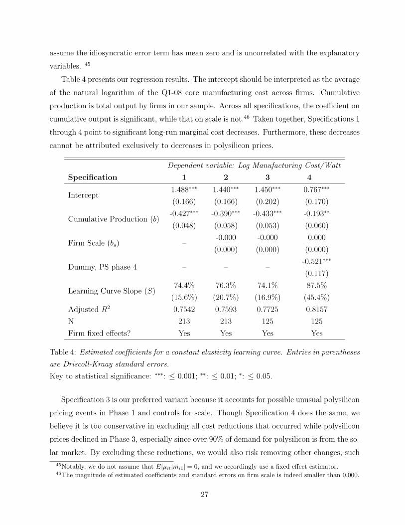
Table 4 presents our regression results. The intercept should be interpreted as the average

of the natural logarithm of the Q1-08 core manufacturing cost across firms. Cumulative

production is total output by firms in our sample. Across all specifications, the coefficient on

cumulative output is significant, while that on scale is not.46 Taken together, Specifications 1

through 4 point to significant long-run marginal cost decreases. Furthermore, these decreases

cannot be attributed exclusively to decreases in polysilicon prices.

Dependent variable: Log Manufacturing Cost/Watt

Specification 1 2 3 4

Intercept1.488∗∗∗

(0.166)

1.440∗∗∗

(0.166)

1.450∗∗∗

(0.202)

0.767∗∗∗

(0.170)

Cumulative Production (b)-0.427∗∗∗

(0.048)

-0.390∗∗∗

(0.058)

-0.433∗∗∗

(0.053)

-0.193∗∗

(0.060)

Firm Scale (bs) –-0.000

(0.000)

-0.000

(0.000)

0.000

(0.000)

Dummy, PS phase 4 – – –-0.521∗∗∗

(0.117)

Learning Curve Slope (S)74.4%

(15.6%)

76.3%

(20.7%)

74.1%

(16.9%)

87.5%

(45.4%)

Adjusted R2 0.7542 0.7593 0.7725 0.8157

N 213 213 125 125

Firm fixed effects? Yes Yes Yes Yes

Table 4: Estimated coefficients for a constant elasticity learning curve. Entries in parentheses

are Driscoll-Kraay standard errors.

Key to statistical significance: ∗∗∗: ≤ 0.001; ∗∗: ≤ 0.01; ∗: ≤ 0.05.

Specification 3 is our preferred variant because it accounts for possible unusual polysilicon

pricing events in Phase 1 and controls for scale. Though Specification 4 does the same, we

believe it is too conservative in excluding all cost reductions that occurred while polysilicon

prices declined in Phase 3, especially since over 90% of demand for polysilicon is from the so-

lar market. By excluding these reductions, we would also risk removing other changes, such

45Notably, we do not assume that E[µit|mi1] = 0, and we accordingly use a fixed effect estimator.46The magnitude of estimated coefficients and standard errors on firm scale is indeed smaller than 0.000.

27

as those in module efficiency and polysilicon utilization, which Pillai (2015) documents as

significant drivers of reductions in COGS. Nonetheless, if one believes either that the polysil-

icon and solar module markets are insufficiently linked or that polysilicon price dynamics are

likely to fundamentally differ from those observed from Q2-09 through Q4-13, Specification

4 provides a more appropriate rate of cost declines for core manufacturing costs.

Finding 4 Controlling for plant scale and excluding periods with large polysilicon price

declines, we estimate a 74% learning curve for core manufacturing costs over the period

2008–2013.

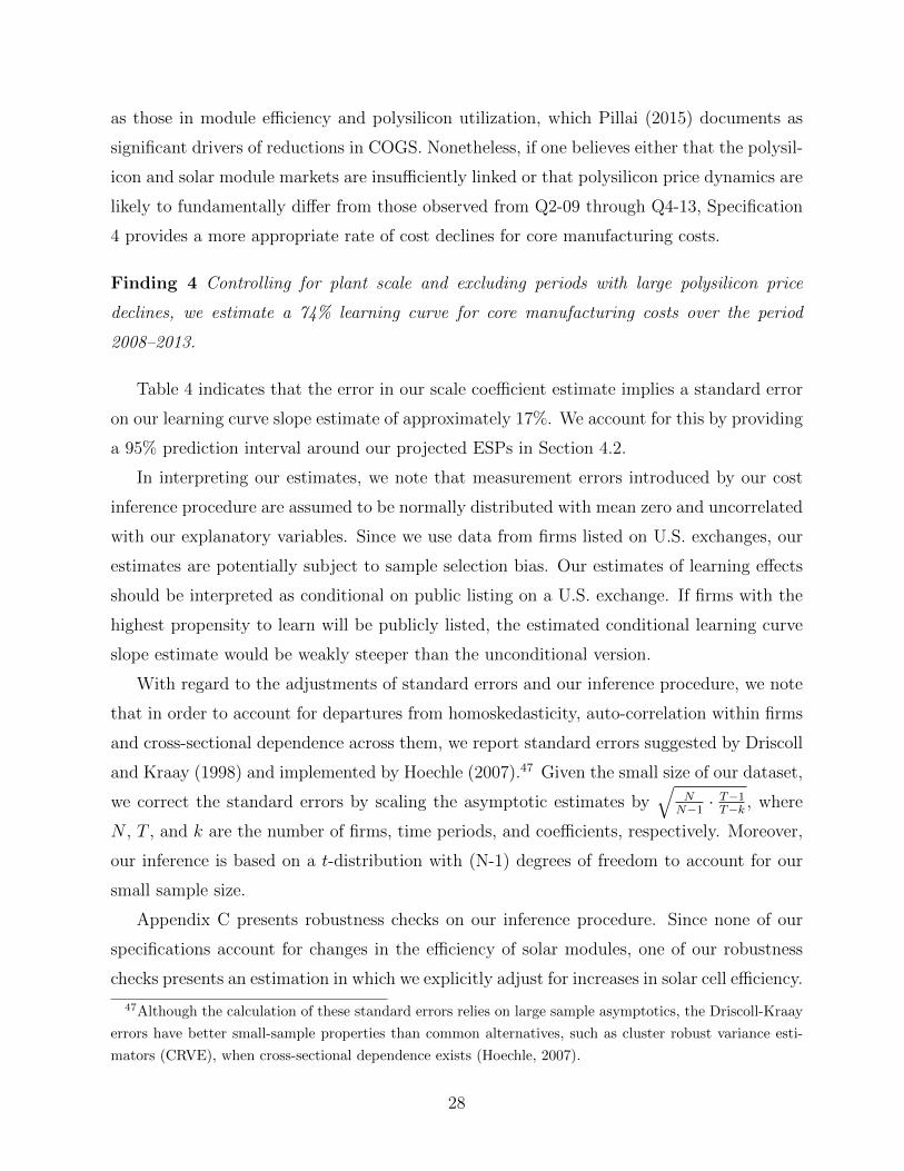
Table 4 indicates that the error in our scale coefficient estimate implies a standard error

on our learning curve slope estimate of approximately 17%. We account for this by providing

a 95% prediction interval around our projected ESPs in Section 4.2.

In interpreting our estimates, we note that measurement errors introduced by our cost

inference procedure are assumed to be normally distributed with mean zero and uncorrelated

with our explanatory variables. Since we use data from firms listed on U.S. exchanges, our

estimates are potentially subject to sample selection bias. Our estimates of learning effects

should be interpreted as conditional on public listing on a U.S. exchange. If firms with the

highest propensity to learn will be publicly listed, the estimated conditional learning curve

slope estimate would be weakly steeper than the unconditional version.

With regard to the adjustments of standard errors and our inference procedure, we note

that in order to account for departures from homoskedasticity, auto-correlation within firms

and cross-sectional dependence across them, we report standard errors suggested by Driscoll

and Kraay (1998) and implemented by Hoechle (2007).47 Given the small size of our dataset,

we correct the standard errors by scaling the asymptotic estimates by√

NN−1· T−1T−k , where

N , T , and k are the number of firms, time periods, and coefficients, respectively. Moreover,

our inference is based on a t-distribution with (N-1) degrees of freedom to account for our

small sample size.

Appendix C presents robustness checks on our inference procedure. Since none of our

specifications account for changes in the efficiency of solar modules, one of our robustness

checks presents an estimation in which we explicitly adjust for increases in solar cell efficiency.

47Although the calculation of these standard errors relies on large sample asymptotics, the Driscoll-Kraay

errors have better small-sample properties than common alternatives, such as cluster robust variance esti-

mators (CRVE), when cross-sectional dependence exists (Hoechle, 2007).

28

Accordingly, output is measured in $/m2, rather than on a $/W basis.

4.2 ESP Projections

Given our estimates of the technological progress parameter, η, pertaining to capacity costs

and the learning curve slope applicable to core manufacturing costs, we are in a position to

project future ESPs. The model framework in Section 2 suggests that ASPs should converge

to the long-run marginal cost over time. However, given our findings in Section 3 indicating

that the industry overinvested in capacity in recent years, market demand needs to “catch

up” to the aggregate manufacturing capacity in place in order for the ESPs to becomes the

market clearing prices. For solar PV modules, it should be kept in mind that the expansion

of aggregate demand has been driven in significant part by public policy that has lowered

the cost of solar system prices to investors.48 To capture the sensitivity of ESP projections

to variations in demand, we present ESP forecasts contingent on annual demand ranging

from 40 GW/year to 60 GW/year.

To form our projections, we assume that a representative firm maintains the 35% share

of global module production that the firms in our sample held in 2012. Accordingly, the in-

crease in “within sample” cumulative production is 0.35 · 40 GW in our base line scenario of

40 GW of annual global deployments. Together with our estimated coefficient on cumulative

production, we derive an expected core manufacturing cost for each year. Our projected ca-

pacity cost for the representative firm reflects a weighted average of firms’ projected capacity

costs for each of the years between 2014 and 2020, with weights determined by a given firm’s

share of 2013 shipments. Finally, we add R&D and SG&A costs that are equal to the 2013

shipment-weighted average of firms’ median R&D and SG&A costs from Q1-08 to Q4-13.

Figure 5 depicts the forecast trajectory of ESPs through 2020. This curve reflects both the

74% learning curve for core manufacturing costs and the 78.5% annual geometric decline in

capacity costs. Given a rate of 40 GW of annual production, we then obtain a 27% reduction

in production costs with every doubling in industry-wide output. This trajectory represents

our benchmark of the industry’s production cost fundamentals and can be interpreted as a

trend-line to which the ASPs are expected to converge over time as market demand catches

up with installed capacity. Table 5 presents sensitivity analysis for our estimates by means

48These support policies include feed-in-tariffs, investment tax credits and renewable energy portfolio

standards.

29

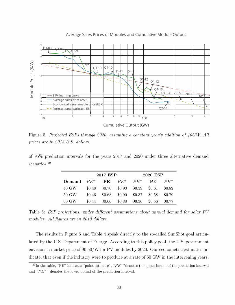
Figure 5: Projected ESPs through 2020, assuming a constant yearly addition of 40GW. All

prices are in 2013 U.S. dollars.

of 95% prediction intervals for the years 2017 and 2020 under three alternative demand

scenarios.49

2017 ESP 2020 ESP

Demand PE− PE PE+ PE− PE PE+

40 GW $0.48 $0.70 $0.93 $0.39 $0.61 $0.82

50 GW $0.46 $0.68 $0.90 $0.37 $0.58 $0.79

60 GW $0.44 $0.66 $0.88 $0.36 $0.56 $0.77

Table 5: ESP projections, under different assumptions about annual demand for solar PV

modules. All figures are in 2013 dollars.

The results in Figure 5 and Table 4 speak directly to the so-called SunShot goal articu-

lated by the U.S. Department of Energy. According to this policy goal, the U.S. government

envisions a market price of $0.50/W for PV modules by 2020. Our econometric estimates in-

dicate, that even if the industry were to produce at a rate of 60 GW in the intervening years,

49In the table, “PE” indicates “point estimate”, “PE+”denotes the upper bound of the prediction interval

and “PE−” denotes the lower bound of the prediction interval.

30

the DOE target is unlikely to be met, if market prices are to cover the long-run marginal

cost. At the same time, we note that in the high-volume 60 GW scenario our ESP point

estimate would miss the $0.50/W goal by a mere 6 cents. Furthermore, the DOE price goal

is covered by our 95% prediction interval in all three demand scenarios as early as 2017. We

also note that, even though our ESP estimates are distinctly above the $0.50/W mark, it is

quite plausible that the aggregate production capacity already in place will cause the ASPs

to exceed the ESPs for several years to come. During that time, the firms in our sample

would then not earn a normal economic profit, though they would rationally continue to

supply modules at prevailing market prices below the ESP.

5 Conclusion

This paper has presented a model framework and an empirical inference procedure for the

long-run marginal cost in an industry characterized by declining production costs. We have

focused our analysis on solar photovoltaic modules, an industry in which a large number of

firms supply a fairly homogeneous product. Our model framework shows that in a dynamic

competitive equilibrium supplier choose their aggregate capacity investments so that the

resulting market prices will in expectation be equal to the declining long-run marginal cost.

Since the corresponding trajectory of market prices would allow firms to recover their periodic

operating- and capacity related costs in the long-run, we refer to these prices as economically

sustainable (ESP).

Our cost inference procedure is based on firm-level financial accounting data, in particular

COGS, SG&A expenses and inventory balances. In addition, we rely on select data from

industry analysts regarding manufacturing capacity and output shipments by individual

firms in our sample. Applying our cost inference method to data from solar PV module

manufacturers enables us to estimate quarterly ESPs and contrast them with observed ASPs.

While our findings suggest that the ASPs and ESPs are statistically indistinguishable for

most of our sample period, they are significantly different in at least four quarters in 2012

and 2013. We conclude that the recently observed price reductions reflect a market dynamic

driven partly by overcapacity rather than mere cost reductions. Furthermore, the resulting

difference between ESPs and ASPs provides a measure of the price effect associated with

excess industry capacity.

Our cost inferences also generate panel data that allow us to extrapolate how the long-run

31

marginal cost of PV modules will change as a function of time and experience. Controlling

for plant scale and significant drops in polysilicon prices, our findings lead to a 74% learning

curve for core manufacturing costs. Combined with our estimates for the annual capacity

cost declines, we arrive at an overall 73% learning curve, implying that the economically

sustainable price drops by 26% with each doubling in cumulative industry output.

The methods and findings of this paper have several immediate policy implications that

could be explored in further research. The pricing of solar PV modules, in particular by

Chinese suppliers, has been challenged on legal grounds in recent years. The complaint of

“dumping” modules is akin to that of predatory pricing in domestic pricing disputes and

generally refers to pricing below cost. Our results indicate that the prices in the 2011-2013

window were frequently below the ESP at the time. Yet, as argued in Section 2, the ESP is

a long-run marginal cost which includes several components that are likely to be considered

“sunk” in the short-run. If the relevant cost benchmark in legal disputes is the short-term

average variable cost, our measure of core manufacturing costs would provide an upper

bound. Our findings give no indication that at any point in time the firms in our sample

were charging prices below their core manufacturing costs .

The demand for solar PV modules over the past decade has in significant part been driven

by public policy support in the form of feed-in-tariffs, investment tax credits and renewable

energy portfolio standards. As solar system prices have dropped rapidly in recent years,

governments in many countries have scaled back these subsidies. For instance, the federal

investment tax credit in the U.S. is currently scheduled to drop from 30% to 10% at the

beginning of 2017. One of the key questions in the current debate is the magnitude of tax

credits required to keep solar power cost competitive with alternative forms of power gener-

ation. The answer to this question hinges in large part on whether the recent acceleration

in cost reductions associated with the production of solar modules is likely to persist.

The research approach taken in this paper is principally applicable in industries other

than solar photovoltaic modules. Our analysis has taken advantage of several features that

apply to the market for PV modules, including a large number of price taking firms, a fairly

homogeneous product and a significant number of “pure play” manufacturers for whom

the production of modules is the dominant line of business. In industries where the latter

condition is not met, our cost inference procedure would be diluted if one were to rely on

firm-wide financial reports. Instead one would need to either aggregate the cost inferences

32

across multiple products or rely on segment reports, e.g, income statement and operating

assets for a particular division within the firm. In industries where firms have significant

pricing power, the analysis in this paper could be enriched by inferring not only the long-run

marginal cost but also examining the price mark-ups that individual firms can charge above

their long-run marginal cost.

33

A Proof of Finding 1

We verify that the sequence of K∗t given by:

P ot (K∗t ) = ESPt ≡ ct ·∆ + wt + ft,

is indeed implementable by a sequence of non-negative investments I∗t if

Kt = It−T + It−T+1 + . . .+ It−1,

and K0 ≤ K∗1 . The non-negativity constraints are met if K∗t+1 ≥ K∗t for t ≥ 1. This follows

from the observation:

P ot+1(K∗t+1) = ESPt+1 < ESPt = P o

t (K∗t ),

combined with the NEC condition requiring that P ot+1(K) > P o

t (K) for all K.

It remains to verify that, given the aggregate capacity levels {K∗t }∞t=1, firms will break-

even on their investments. Without loss of generality, assume that a particular firm invests

in one unit of capacity at time t. The prevailing equilibrium market price in the next T

periods is given by P ot+τ (K

∗t+τ ) = ESPt+τ , with τ ∈ [1, T ]. The firm utilizes this capacity

over the next T periods and the pre-tax cash flows of the investment are given by:

CFLt = −v · ηt,

and for 1 ≤ τ ≤ T ,

CFLt+τ = ESPt+τ − wt+τ − ft+τ = ct+τ ·∆

since, by definition, ESPt = wt + ft + ct ·∆. Taxable income in period t+ τ becomes:

It+τ = CFLt+τ − dτ · v · ηt.

Given a corporate income tax rate of α, the overall NPV of the investment is:

NPVt =T∑τ=1

[CFLt+τ − α · It+τ ] γτ − ηt · v. (26)

34

To see that the expression in (26) is indeed zero, we substitute the expressions for CFLt+τ

and It+τ :

NPVt = (1− α) ·T∑τ=1

∆ · ct+τ · γτ + α ·T∑τ=1

dτ · ηt · v · γτ − ηt · v. (27)

The second term on the right-hand side of (27) denotes the depreciation tax shield. Dividing

by 1− α and collecting terms yields:

1

(1− α)·NPVt = ∆ ·

T∑τ=1

ct+τ · γτ − ηt · v

1− α ·T∑τ=1

dτ · γτ

1− α

. (28)

The tax-factor, ∆, was defined in the main text as:

∆ =

1− α ·T∑τ=1

dτ · γτ

1− α. (29)

Therefore equation (28) reduces to:

1

(1− α)·NPVt = ∆

[T∑τ=1

ct+τ · γτ − ηt · v

].

It remains to show that NPVt = 0, which follows from the construction of the unit cost

of capacity because:

T∑τ=1

ct+τ · γτ ≡T∑τ=1

ηt+τ · vT∑j=1

(γ · η)j· γτ = ηt · v.

35

B Data and adjustments for cost inferences

Firms in the study set

Firm Ticker 2012 Capacity % 2012 Production %

Yingli Green Energy NYSE: YGE 3.7 6.4

Trina Solar NYSE: TSL 3.7 4.6

Suntech Power NYSE: STP 4.0 5.9

Canadian Solar NASDAQ: CSIQ 3.4 4.8

LDK Solar NYSE: LDK 2.7 1.5

Hanwha Solar One NASDAQ: HSOL 2.4 2.6

JA Solar NASDAQ: JASO 3.3 3.6

ReneSola NYSE: SOL 1.6 1.7

JinkoSolar NYSE: JKS 1.9 2.7

China Sunergy NASDAQ: CSUN 1.3 1.1

Table 6: Firms included in the study set, including stock tickers, capacity, and market share

as of 2012.

Price data

Since prominent sources of module price data (i.e., Bloomberg New Energy Finance and

pvXchange) began collecting price data no earlier than Q3-09, the average sales price (ASP)

measure we use in our graphs is a composite of several indexes. The measure equally weighs

our estimates of in-sample ASPs and a composite of price indexes that we obtain either from

Swanson (2011) or the Bloomberg terminal system. For each firm and quarter, we derive

firm-specific ASPs as the quotient of revenues and the sales volume:

ASPit(firm− specific) =RevenueitsMEit

(30)

This implies a quarter-specific average in-sample ASP:

ASPt(in− sample) =∑i

witASPit, (31)

where the weights in the above summation are in proportion to the firm’s share of module-

equivalent shipments across the firms in our sample in that quarter.

Our composite of indexes reflects the data available for a particular period. Prior to

Q1-10, we use price data included in Swanson (2011). After Q4-10, we use a Bloomberg

36

New Energy Finance index for multi-crystalline silicon module prices. To bridge the gap

between the data from Swanson and that available from BNEF, we use the pvXchange

Crystalline Modules China Price available from the Bloomberg terminal. We chose this index

for Q1-10 through Q3-10 among those from PVXchange and PVinsights and accessible from

the Bloomberg terminal system because it offered the best match with the BNEF multi-

crystalline silicon module price index over the time periods in which we could observe both

indexes. The ASPs on our graphs equal the simple average of our composite index and

in-sample ASP measures.

In contrast, our tests about whether the market is in long-run equilibrium in a given

quarter use only the firm-specific ASP estimates. By using the firm-specific ASP estimates,

we can compare a distribution of estimated ASPs and inferred ESPs across firms. We observe

a relatively close match between our in-sample ASPs and the index price data; across the 24

quarters in our sample, we observe a median difference of 12% between the two numbers.

Adjusting facility capacity costs for physical efficiency gains

As the efficiency of solar cells increases, the same physical area of output contains a

greater Watt capacity and therefore the capacity cost per Watt decreases. Recalling that

ηf = 1, we modify cft from its form in (16) to:

cft =vf · effrefefft∑30

τ=1 γτ.

Here, efft and effref refer to average efficiency levels in the current and baseline periods,

respectively. Table 7 shows data from Fraunhofer (2012) which we use to adjust our capacity

cost estimates. Our estimated facility cost estimates in Table 2 for 2013 through 2016 reflect

assumptions about efficiency levels. Given reports by Fraunhofer that 2014 average efficiency

levels had reached 16%, we assume a 15.5% efficiency level in 2013 and a steady 16% efficiency

level thereafter.

2003 2004 2005 2006 2007 2008 2009 2010 2011 2012

12.0% 12.5% 12.5% 12.7% 13.0% 13.1% 13.1% 13.4% 14.5% 14.7%

Table 7: Average crystalline silicon module efficiency, from Fraunhofer (2012).

37

Deriving module-equivalent capacity

In Section 3.1.2, we discuss two adjustments to the measure of firm-specific equipment

capacity costs. One modification adjusts the level of capacity additions by firms. The naive

approach implied by (17) assumes that a firm’s capital expenditures on equipment are solely

applied to the expansion of module manufacturing capacity. However, firms could have

expanded capacity for any of the four steps of module manufacturing or any combination

thereof. In practice, firms have tended to invest in capacity either for only one of the four

steps or for combinations of the four steps that are contiguous to each other and include

all upstream steps. The latter observation implies that firms have invested in, for example,

cell, wafer, and ingot capacity but not in only cell and ingot capacity. This practical reality

implies that there are ten types of what we term contiguous capacity investment bundles.50

Of course, it is not equally costly to expand each of the ten capacity bundles. To account

for these differences, we use a module-equivalent (ME) level of capacity, KME:

KME = Σl=10l=1 Kj · χj (32)

Here, the index j refers to the ten contiguous capacity investment bundles. We use quarterly

firm-level capacity data from Lux Research (2014) across all steps of the value chain to

derive Kj and KME.51 We determine the expansion of a particular bundle by (1) taking the

minimum of the capacity expansions for all constituent value chain steps and (2) subtracting

the expansions recorded for more inclusive bundles. As an example, when calculating the

capacity expansion in the “cells and modules” bundle, we know that this increase cannot

exceed the observed expansion of either cell or module capacity (i.e., the constituent value

chain steps). We thus calculate the minimum capacity expansion level observed across these

50The ten bundles are investments in (1) ingots only, (2) wafers only, (3) cells only, (4) modules only, (5)

wafers and ingots, (6) cells, wafers, and ingots, (7) cells and wafers, (8) modules, cells, wafers, and ingots,

(9) modules, cells, wafers, and (10) modules and cells.51We make several amendments to the records in this dataset based on our findings from firms’ press

releases and industry analysts. For Yingli, we use a 2014 module capacity of 2.45GW because we exclude

tolling facilities to which the firm had access. For JA Solar, we added 150MW of module capacity in 2014 that

stem from new capacity in South Africa but not included in the Lux Research dataset. For China Sunergy,

we use an 1.155GW module capacity figure reported by Bloomberg New Energy Finance that matches with

numbers released by the firm itself. Finally, we use 800MW for Hanwha SolarOne’s ingot capacity; while

Lux Research (2014) does not include any ingot manufacturing capacity for this firm, previous versions of

the same dataset record an ingot capacity of 800MW per year. In addition, the firm reports that it operates

ingot manufacturing capacity.

38

two steps. To avoid double counting capacity expansions in cells and modules, we subtract

the capacity expansion observed across the two more inclusive bundles, namely “modules,

cells, wafers, and ingots” and “modules, cells, and wafers.”

χj is an adjustment factor that “marks down” the capacity additions for bundles that do

not include all four components of the value chain. We define χj as the ratio of the capacity

cost for bundle j to the capacity cost for the integrated module capacity investment. We

estimate χj as the average of the ratios from 2009 to 2016 implied by Table 2.

C Learning curve estimation robustness checks

Accounting for physical efficiency gains

Since a time trend would have accounted for core manufacturing cost reductions due to

improved quality, as measured by physical efficiency, we repeat Specifications 1 through 4

with data expressed on a dollar per square meter basis. We represent the effect of efficiency

improvements in solar cells via the metric efficiency = powerm2 . Accordingly, we convert

manufacturing costs from dollars per Watt to dollars per square meter by multiplying the

former by efficiency. We use average module efficiency levels from Table 7 and change the

scale and cumulative output measures to a square meter basis. Table 8 summarizes our

estimates; each specification corresponds to the numbering in Table 4.

Comparing Tables 4 and 8, we observe that the implied learning curve slopes are essen-

tially the same across the two tables, with the slopes on a $/Watt basis roughly up to 1 –

2% steeper than those on a $/m2 basis. The estimates suggest that our results are robust

to the specification of output on an efficiency-adjusted basis.

39

Dependent variable: Log Manufacturing Cost/m2

Specification 1SM 2SM 3SM 4SM

Intercept-0.604∗∗∗

(0.155)

-0.632∗∗∗

(0.155)

-0.689∗∗∗

(0.183)

-1.273∗∗∗

(0.146)

Cumulative Production (b)-0.391∗∗∗

(0.044)

-0.367∗∗∗

(0.053)

-0.395∗∗∗

(0.048)

-0.188∗∗

(0.053)

Firm Scale (bs) –-0.000

(0.000)

-0.000

(0.000)

0.000

(0.000)

Dummy, PS phase 4 – – –-0.431∗∗∗

(0.106)

Learning Curve Slope (S)76.3%

(15.7%)

77.5%

(20.0%)

76.1%

(16.7%)

87.8%

(41.2%)

Adjusted R2 0.7273 0.7297 0.7337 0.7784

N 213 213 125 125

Firm fixed effects? Yes Yes Yes Yes

Table 8: Estimated coefficients on a constant elasticity learning curve. Entries in parentheses

are Driscoll-Kraay standard errors.

Key to statistical significance: ∗∗∗: ≤ 0.001; ∗∗: ≤ 0.01; ∗: ≤ 0.05.

Exclusion of firm-quarter pairs

Since some firms had a small share of modules in their output mix over some of the

periods in our panel, we conducted four robustness checks in which we exclude observations

for these firms in such periods. In the first, we drop data from CSUN between Q1-08 and

Q3-10. The second drops data from JASO between Q1-08 and Q4-11, while the third drops

data from SOL between Q1-08 and Q3-10. Finally, we drop all three sets of observations.

We do not list the estimates derived upon dropping these observations, but we do not find

any material differences between the learning curve slopes estimated from the full sample

and those obtained when using the restricted samples. Though the standard errors change,

they do not change in a systematic direction with these exclusions.

40

References

Abel, A., and J. Eberly (2011), “How Q and Cash Flow Affect Investment Without Friction:

An Analytic Explanation,” Review of Economic Studies, 78, 1179–1200.

Afshartous, D., and R. A. Preston (2010), “Confidence intervals for dependent data: equat-

ing non-overlap with statistical significance,” Computational Statistics & Data Analysis,

54(10), 2296–2305.

Arrow, K. (1964), “Optimal Capital Policy, The Cost of Capital and Myopic Decision Rules,”

Annals of the Institute of Statistical Mathematics, 1-2, 21 – 30.

Balakrishnan, R., and K. Sivaramakrishnan (2002), “A Critical Overview of Full-Cost Data

for Planning and Pricing.” Journal of Management Accounting Research, 14, 3–31.

Baldenius, T., A. Nezlobin, and I. Vaysman (2015), “Managerial Performance Evaluation

and Real Options,” The Accounting Review (forthcoming).

Banker, R. D., and J. S. Hughes (1994), “Product Costing and Pricing.” The Accounting

Review, 69, 479–494.

Candelise, C., M. Winskel, and R. J. Gross (2013), “The dynamics of solar PV costs and

prices as a challenge for technology forecasting,” Renewable and Sustainable Energy Re-

views, 26, 96–107.

Carlton, D. W., and J. M. Perloff (2005), Modern Industrial Organization., 4th ed., Pear-

son/Addison Wesley, New York.

Dick, A. R. (1991), “Learning by Doing and Dumping in the Semiconductor Industry,”

Journal of Law and Economics, 34(1), pp. 133–159.

Driscoll, J. C., and A. C. Kraay (1998), “Consistent Covariance Matrix Estimation with

Spatially Dependent Panel Data,” Review of Economics and Statistics, 80(4), 549–560.

Dutta, S., and S. Reichelstein (2010), “Decentralized Capacity Management and Internal

Pricing,” Review of Accounting Studies, 15(3), 442 – 478.

Fraunhofer (2012), “Photovoltaics Report,” Tech. rep., Fraunhofer Institute for Solar Energy

Systems.

41

Goodrich, A., P. Hacke, Q. Wang, B. Sopori, R. Margolis, T. L. James, and M. Woodhouse

(2013a), “A wafer-based monocrystalline silicon photovoltaics road map: Utilizing known

technology improvement opportunities for further reductions in manufacturing costs,” So-

lar Energy Materials and Solar Cells, 114, 110–135.

Goodrich, A. C., D. M. Powell, T. L. James, M. Woodhouse, and T. Buonassisi (2013b),

“Assessing the Drivers of Regional Trends in Solar Photovoltaic Manufacturing,” Energy

& Environmental Science, 6, 2811 – 2821.

Gox, R. (2002), “Capacity Planning and Pricing under Uncertainty.” Journal of Management

Accounting Research, 14, 59–78.

Greene, W. H. (2003), Econometric Analysis, Pearson.

GTM (2012), “GTM Research PV Technology, Production and Cost Outlook: 2012 – 2016,”

Tech. rep.

Hoechle, D. (2007), “Robust Standard Errors for Panel Regressions with Cross-Sectional

Dependence,” Stata Journal, 7(3), 281.

Lazard, P. (2009), “Levelized Cost of Energy Analysis,” Tech. rep., Lazar Capital Markets

Report, version 3.

Lieberman, M. B. (1984), “The Learning Curve and Pricing in the Chemical Processing

Industries,” The RAND Journal of Economics, 15(2), 213 – 228.

Lux Research (2012a), “Q4 2012 Supply Tracker,” Available by subscription to Lux Research.

Lux Research (2012b), “Turning Lemons into Lemonade: Opportunities in the Turbulent

PV Equipment Market,” Available by subscription to Lux Research.

Lux Research (2014), “Q1 2014 Supply Tracker,” Available by subscription to Lux Research.

Narayanan, V. (2003), “Activity-based pricing in a Monopoly.” Journal of Accounting Re-

search, 41, 473–502.

Nezlobin, A. (2012), “Accrual Accounting, Informational Sufficiency, and Equity Valuation,”

Journal of Accounting Research.

42

Nezlobin, A., M. V. Rajan, and S. Reichelstein (2012), “Dynamics of Rate-of-Return Regu-

lation,” Management Science, 58(5), 980–995.

Pillai, U. (2015), “Drivers of cost reduction in solar photovoltaics,” Energy Economics, 50,

286–293.

Pillai, U., and J. McLaughlin (2013), “A model of competition in the solar panel industry,”

Energy Economics, 40, 32–39.

Pittman, B. (2009), “Whom Are You Calling Irrational? Marginal Costs, Variable Costs,

and the Pricing Practices of Firms,” Working Paper, Department Of Justice, Washington

DC.

Powell, D., M. Winkler, H. Choi, C. Simmons, D. Needleman, and T. Buonassisi (2012),

“Crystalline silicon photovoltaics: a cost analysis framework for determining technology

pathways to reach baseload electricity costs,” Energy & Environmental Science, 5, 5874 –

5883.

Powell, D., M. Winkler, A. Goodrich, and T. Buonassisi (2013), “Modeling the Cost and Min-

imum Sustainable Price of Crystalline Silicon Photovoltaic Manufacturing in the United

States,” IEEE Journal of Photovoltaics.

PWC (2012), “Financial Engineering as a Means to Support Jawaharlal Nehru Solar Mis-

sion,” Tech. rep., PWC.

Rajan, M., and S. Reichelstein (2009), “Depreciation Rules and The Relation Between

Marginal and Historical Cost,” Journal of Accounting Research, 47, 1 – 43.

Reichelstein, S., and A. Rohlfing-Bastian (2015), “Levelized Product Cost: Concept and

Decision Relevance,” The Accounting Review, 55, 117 – 127.

Reichelstein, S., and M. Yorston (2013), “The Prospects for Cost Competitive Solar PV

Power,” Energy Policy, 90(4), 1653 – 1682.

Rogerson, W. (2008), “Inter-Temporal Cost Allocation and Investment Decisions,” Journal

of Political Economy, 116, 931 – 950.

Rogerson, W. (2011), “On the Relationship between Historic Cost, Forward Looking Cost

and Long Run Marginal Cost,” Review of Network Economics, 10(2).

43

Spence, A. M. (1981), “The learning curve and competition,” The Bell Journal of Economics,

49–70.

Stobaugh, R. B., and P. L. Townsend (1975), “Price forecasting and strategic planning: the

case of petrochemicals,” Journal of Marketing Research, 19–29.

Swanson, R. (2011), “The Silicon Photovoltaic Roadmap,” The Stanford Energy Seminar.

44