cost-effective strategy to mitigate transportation...
TRANSCRIPT
THESIS – TI 42307 Cost-effective Strategy to Mitigate Transportation Disruption in Supply Chain
Gustav Albertzeth 2515206342 SUPERVISOR
Prof. Ir. I Nyoman Pujawan, M.Eng., Ph.D., CSCP MASTER PROGRAM
OPERATIONS AND SUPPLY CHAIN ENGINEERING
DEPARTMENT OF INDUSTRIAL ENGINEERING
FACULTY OF INDUSTRIAL TECHNOLOGY
INSTITUT TEKNOLOGI SEPULUH NOPEMBER
SURABAYA
2017

This page is intentionally left blank

i
STATEMENT OF AUTHENTICITY
I, the undersigned,
Name : Gustav Albertzeth
NRP : 2515206342
Study Program : Master Program of Industrial Engineering
Declare that my thesis entitled:
“COST-EFFECTIVE STRATEGY TO MITIGATE TRANSPORTATION DISRUPTION IN SUPPLY CHAIN”
Is a complete independent work of mine, completed without using any illegal
information, nor the work of others that I recognize as my own work.
All cited and references are listed in the bibliography.
If it turns out that this statement is not true, I am willing to accept the
consequences in accordance with the regulations.
Surabaya, July 19th 2017 Sincerely,
Gustav Albertzeth 2515206342

ii
This page is intentionally left blank
iii
ACKNOWLEDGEMENTS
God is good, God is great! Only by His grace I had the privilege of working
with a number of people who gave me support and encouragement throughout the
Master Program and made it enjoyable. I wish to express my gratitude to these
people. First and foremost, I would like to thank my supervisor Prof. Ir. I Nyoman
Pujawan, M.Eng., Ph.D., CSCP. for being an important source of guidance and
direction throughout the whole progress of my thesis. His encouragement and help
greatly help the writings and the publication of my thesis.
I also wish to thank the examiners during my thesis defense presentation,
Mr. Erwin Widodo, S.T., M.Eng., Dr.Eng. and Mrs. Niniet Indah Arvitrida, S.T.,
M.T., Ph.D. who have provided me with valuable opinions and corrections on the
full completion of my thesis
I would also like to thank my fellow students, Ibrahim Musa and Cindy
Revitasari, with whom I have had opportunities to exchange opinions and
information regarding the work of my thesis. In particular, to Thomas Indarto
Wibowo for the stimulating conversation we had, that leads to the elementary idea
of my thesis. I am also grateful to Mr. Kis Dwiantoro, Mr. Rahmat Syam, Mr. Albert
Kareba, and Mrs. Kasmawati who have helped me with an access to the database
for the sample of this thesis as well as providing practical advices in data collection.
I would also show my gratitude for my lecturers in Atma Jaya Yogyakarta
University (UAJY), especially Mr. The Jin Ai, S.T., M.T., D.Eng., Mr. Yosef
Daryanto, S.T., M.Sc., and Mrs. L. Bening Parwitasukci, S.Pd, M.Hum. for kindly
providing me with their supportive recommendations in the application for my
Master Program, without which the opportunity to undertake Master Study at this
university would have never been possible.
Finally, I also thank my family for being a major source of support that has
sustained me during the completion of this study. My mother, Elsje Saimima, has
not only been understanding but also very supportive, often making considerable
personal sacrifices for the demands the study has made on my time. My brother,
Yean Aguste, who has encouraged to pursue my education in ITS Surabaya.

iv
.
This page is intentionally left blank

v
COST-EFFECTIVE STRATEGY TO MITIGATE TRANSPORTATION DISRUPTION IN SUPPLY CHAIN
By : Gustav Albertzeth NRP : 2515206342 Supervisor : Prof. Ir. I Nyoman Pujawan, M.Eng., Ph.D., CSCP
ABSTRACT
Phenomena of disruption events in supply chain have gained many attractions by scholars. Even though transportation plays a central role in supply chain, studies in transportation disruption has received little attention. This research simulates a model of order delivery process from a focal company (FC) to a single distributor, where a transportation disruption stochastically occurs. Considering the possibility of sales loss during the disruption duration, we proposed a redundant stock, flexible route, and combined flexibility-redundancy (ReFlex) as mitigation strategies and a base case as a risk acceptance strategy. The objective is to find out the best strategy that promote cost-effectiveness against transportation disruption. In the base case, delivery process was halt during the disruption duration and resumed as soon as the road has been fixed. In the redundant stock situation, FC placed an extra stock in distributor’s warehouse that act as a buffer against stockouts. In flexible route, FC use an alternative route for the delivery process only when disruption occurred. In ReFlex, when disruption occurs, not only that alternative route was taken, but also an extra stock in distributor’s warehouse was placed to protect against stockouts. We ran the simulation model using these strategies for 5 brands. We found that the proposed mitigation strategies were having the capability to negate the impact of transportation disruption, each with its own cost and effectiveness, while accepting the risk caused the greatest loss. We found that redundant stock gave the best effectiveness against disruption for all brands, ReFlex as the second best, while flexible route gave the least effectiveness. We also found through sensitivity analysis that ReFlex has the potential to become the best option with buffer stock quantity improvement. Finally, through cost-effectiveness analysis (CEA) we gave recommendations of which strategy should be applied based on the decision maker willingness to pay. Keywords: Transportation disruption, mitigation strategy, redundant stock, flexible route, simulation modeling, cost-effectiveness analysis

vi
This page is intentionally left blank
vii
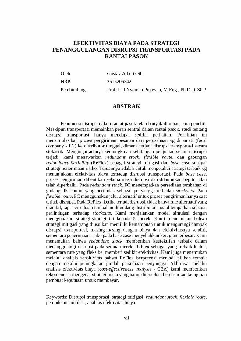
EFEKTIVITAS BIAYA PADA STRATEGI PENANGGULANGAN DISRUPSI TRANSPORTASI PADA
RANTAI PASOK
Oleh : Gustav Albertzeth NRP : 2515206342 Pembimbing : Prof. Ir. I Nyoman Pujawan, M.Eng., Ph.D., CSCP
ABSTRAK
Fenomena disrupsi dalam rantai pasok telah banyak diminati para peneliti. Meskipun transportasi memainkan peran sentral dalam rantai pasok, studi tentang disrupsi transportasi hanya mendapat sedikit perhatian. Penelitian ini mensimulasikan proses pengiriman pesanan dari perusahaan yg di amati (focal company - FC) ke distributor tunggal, dimana terjadi disrupsi transportasi secara stokastik. Mengingat adanya kemungkinan kehilangan penjualan selama disrupsi terjadi, kami menawarkan redundant stock, flexible route, dan gabungan redundancy-flexibility (ReFlex) sebagai strategi mitigasi dan base case sebagai strategi penerimaan risiko. Tujuannya adalah untuk mengetahui strategi terbaik yg menunjukkan efektivitas biaya terhadap disrupsi transportasi. Pada base case, proses pengiriman dihentikan selama masa disrupsi dan dilanjutkan begitu jalan telah diperbaiki. Pada redundant stock, FC menempatkan persediaan tambahan di gudang distributor yang bertindak sebagai penyangga terhadap stockouts. Pada flexible route, FC menggunakan jalur alternatif untuk proses pengiriman hanya saat terjadi disrupsi. Pada ReFlex, ketika terjadi disrupsi, tidak hanya rute alternatif yang diambil, tapi persediaan tambahan di gudang distributor juga ditempatkan sebagai perlindugan terhadap stockouts. Kami menjalankan model simulasi dengan menggunakan strategi-strategi ini kepada 5 merek. Kami menemukan bahwa strategi mitigasi yang diusulkan memiliki kemampuan untuk mengurangi dampak disrupsi transportasi, masing-masing dengan biaya dan efektivitasnya sendiri, sementara penerimaan risiko pada base case menyebabkan kerugian terbesar. Kami menemukan bahwa redundant stock memberikan keefektifan terbaik dalam menanggulangi disrupsi pada semua merek, ReFlex sebagai yang terbaik kedua, sementara rute yang fleksibel memberi sedikit efektivitas. Kami juga menemukan melalui analisis sensitivitas bahwa ReFlex berpotensi menjadi pilihan terbaik dengan melalui peningkatan jumlah persediaan penyangga. Akhirnya, melalui analisis efektivitas biaya (cost-effectiveness analysis - CEA) kami memberikan rekomendasi mengenai strategi mana yang harus diterapkan berdasarkan keinginan pembuat keputusan untuk membayar. Keywords: Disrupsi transportasi, strategi mitigasi, redundant stock, flexible route, pemodelan simulasi, analisis efektivitas biaya

viii
This page is intentionally left blank

ix
TABLE OF CONTENTS
STATEMENT OF AUTHENTICITY ...................................................................i
ACKNOWLEDGEMENTS ................................................................................ iii
ABSTRACT ........................................................................................................... v
ABSTRAK .......................................................................................................... vii
TABLE OF CONTENTS .....................................................................................ix
LIST OF FIGURES ............................................................................................ xv
LIST OF TABLES ............................................................................................ xvii
CHAPTER 1 INTRODUCTION .......................................................................... 1
1.1. Background ....................................................................................................... 1
1.2. Research Questions ........................................................................................... 3
1.3. Research Objectives .......................................................................................... 3
1.4. Benefits ............................................................................................................. 3
1.5. Research Limitation .......................................................................................... 3
1.6. Assumptions ...................................................................................................... 4
1.7. Thesis Structure ................................................................................................ 4
CHAPTER 2 LITERATURE REVIEW .............................................................. 7
2.1. Supply Chain ..................................................................................................... 7
2.1.1. Competitive Advantage ..................................................................... 8
2.1.2. Supply Chain Vulnerability ............................................................. 10
2.1.3. The Role of Transportation in Supply Chain ................................... 10

x
2.2. Supply Chain Disruption ................................................................................. 11
2.2.1. Transportation Disruption ............................................................................ 11
2.3. Responses Against Disruption ........................................................................ 13
2.3.1. Risk Acceptance ............................................................................... 13
2.3.2. Risk Shifting .................................................................................... 14
2.3.3. Risk Mitigation ................................................................................ 15
2.4. Simulation Modeling ...................................................................................... 17
2.4.1. Application of Simulation in Risk Management ............................. 19
2.4.2. Conducting Simulation Study .......................................................... 19
2.5. Cost-Effectiveness Analysis (CEA) ................................................................ 23
2.5.1. Incremental Cost-Effectiveness Ratio (ICER) ................................. 25
2.5.2. Application of Cost-Effectiveness in Risk Management ................. 26
2.6. Research Gap ............................................................................................. 27
CHAPTER 3 RESEARCH METHODS ............................................................ 29
3.1. Research Framework ...................................................................................... 29
3.2. Methods on Simulation Modeling .................................................................. 30
3.2.1. Data collection ................................................................................. 31
3.2.2. Model translation ............................................................................. 31
3.2.3. Verification and Validation (V&V) ................................................. 32
3.2.4. Experimental Design ........................................................................ 33
3.2.5. Production Runs and Analysis ......................................................... 33
3.2.6. More Runs ........................................................................................ 33
3.3. Methods on CEA ............................................................................................. 36

xi
CHAPTER 4 DATA COLLECTION ................................................................. 39
4.1. Relationship Between Focal Company and Distributor .................................. 39
4.2. Collected Data on FGSC Department ............................................................. 40
4.3. Data Collected on Procurement Department .................................................. 47
4.4. Data collected on Sales Department ............................................................... 49
4.5. Data Collected on BNPB ................................................................................ 49
4.6. Proposed Strategies and Impact Costs ............................................................ 50
4.6.1. Base Case ......................................................................................... 50
4.6.2. Redundant Stock .............................................................................. 51
4.6.3. Flexible Route .................................................................................. 51
4.6.4. ReFlex .............................................................................................. 52
CHAPTER 5 SIMULATION STUDY & CEA ................................................. 53
5.1. Simulation Study ............................................................................................. 53
5.1.1. Problem Formulation ....................................................................... 53
5.1.2. Setting Objectives ............................................................................ 53
5.1.3. Model Conceptualization ................................................................. 53
5.1.4. Simulation Inputs Formulation ........................................................ 56
5.1.5. Computerized Model in ARENA ..................................................... 57
5.1.6. Verification ...................................................................................... 63
5.1.7. Validation ......................................................................................... 65
5.1.8. Sensitivity Analysis ......................................................................... 66
5.1.9. Production Run & Output Analysis ................................................. 66
5.1.10. Replications .................................................................................... 67
5.1.11. Document Cost and Effectiveness ................................................. 67

xii
5.2. Cost-Effectiveness Analysis ........................................................................... 70
5.2.1. Obtain cost and effectiveness from simulation study ...................... 70
5.2.2. List Strategies in Ascending Order .................................................. 71
5.2.3. Identify Weakly and/or Strongly Dominated Strategy .................... 71
5.2.4. Calculate ICER ................................................................................ 71
5.2.5. Identify Extended Dominated Strategy ............................................ 72
5.2.6. Introduce Initial Recommendation .................................................. 73
CHAPTER 6 ANALYSIS & FINDINGS ........................................................... 75
6.1. Sensitivity Analysis ........................................................................................ 75
6.2. Findings on Brand A ....................................................................................... 76
6.2.1. Factors and Responses Relationship ................................................ 76
6.2.2. Final Recommendation .................................................................... 77
6.3. Findings on Brand B ....................................................................................... 78
6.3.1. Factors and Responses Relationship ................................................ 79
6.3.2. Final Recommendation .................................................................... 80
6.4. Findings on Brand C ....................................................................................... 81
6.4.1. Factors and Responses Relationship ................................................ 81
6.4.2. Final Recommendation .................................................................... 82
6.5. Findings on Brand D ....................................................................................... 83
6.5.1. Factors and Responses Relationship ................................................ 84
6.5.2. Final Recommendation .................................................................... 85
6.6. Findings on Brand E ....................................................................................... 86
6.6.1. Factors and Responses Relationship ................................................ 86
6.6.2. Final Recommendation .................................................................... 87

xiii
6.7 Analysis on Findings ........................................................................................ 88
6.7. Comparison of Findings with Previous Research .......................................... 92
CHAPTER 7 CONCLUSIONS & CONTRIBUTIONS ................................... 93
7.1. Conclusions ..................................................................................................... 93
7.2. Contributions ................................................................................................... 93
7.2.1. Academic Field ................................................................................ 94
7.2.2. Managerial Implication .................................................................... 94
7.2.3. Potential Future Research ................................................................ 94
REFERENCES ..................................................................................................... 95
APPENDICES .................................................................................................... 103
Appendix A: Example of Verification for Base Case Strategy on Brand E ........ 103
Appendix B: Example of Simulation Input for Brand E ...................................... 107
Appendix C: Example of Simulation Report for Brand E ................................... 111
AUTHOR’S BIOGRAPHY ............................................................................... 115

xiv
This page is intentionally left blank

xv
LIST OF FIGURES
Figure 2.1 Supply chain as a network of companies............................................... 7
Figure 2.2 Network between companies creates stages in supply chain ................ 8
Figure 2.3 The value chain activities ...................................................................... 9
Figure 2.4 12 Steps in simulation study ................................................................ 20
Figure 3.1 Research Framework ............................................................................ 29
Figure 3.2 First construct of the research framework ............................................ 30
Figure 3.3 Methods to conduct simulation study for this research ....................... 35
Figure 3.4 Second construct of the research framework ........................................ 36
Figure 3.5 ICER effective algorithm as method to conduct CEA ........................ 38
Figure 4.1 The Supply Chain of Focal Company ................................................. 40
Figure 4.2 Delivery schedule obtained from FC .................................................... 46
Figure 4.3 Primary route Makassar- Poso ............................................................. 47
Figure 4.4 Travel route from Makassar to Mamuju ............................................... 48
Figure 4.5 Travel route from Mamuju to Poso ...................................................... 48
Figure 5.1 Computerized model for base case strategy ........................................ 59
Figure 5.2 Computerized model for redundant stock strategy .............................. 60
Figure 5.3 Computerized model for flexible route strategy .................................. 61
Figure 5.4 Computerized model for ReFlex strategy ............................................ 62
Figure 5.5 Output comparison of hand calculations (top) with computerized model
(bottom) on base case ............................................................................................. 63

xvi
Figure 5.6 Output comparison of hand calculations (top) with computerized model
(bottom) on redundant stock strategy .................................................................... 64
Figure 5.7 Output comparison of hand calculations (top) with computerized model
(bottom) on flexible strategy .................................................................................. 64
Figure 5.7 Output comparison of hand calculations (top) with computerized model
(bottom) on ReFlex strategy .................................................................................. 65
Figure 6.1 Comparison between initial recommendation (top) with final
recommendation (below) for brand A .................................................................... 89
Figure 6.2 Comparison between initial recommendation (top) with final
recommendation (below) for brand B .................................................................... 89
Figure 6.3 Comparison between initial recommendation (top) with final
recommendation (below) for brand C .................................................................... 89
Figure 6.4 Comparison between initial recommendation (top) with final
recommendation (below) for brand D .................................................................... 90
Figure 6.5 Comparison between initial recommendation (top) with final
recommendation (below) for brand E .................................................................... 90
Figure 6.6 Graph of cost-effectiveness pattern between brands ............................ 91
Figure 6.7 Cost-effectiveness of mitigation strategy relative to demand rate ........ 91

xvii
LIST OF TABLES
Table 2.1 Previous research in transportation disruption ...................................... 28
Table 4.1 Delivered brands during the year of 2016 ............................................. 42
Table 4.2 Delivery details for brand A .................................................................. 42
Table. 4.3 Delivery details for brand B .................................................................. 43
Table. 4.4 Delivery details for brand C .................................................................. 43
Table. 4.5 Delivery details for brand D ................................................................. 44
Table. 4.6 Delivery details for brand E .................................................................. 44
Table 4.7 Days between order and estimated demand for brand A ....................... 45
Table 4.8 Days between order and estimated demand for brand B ....................... 45
Table 4.9 Days between order and estimated demand for brand C ....................... 45
Table 4.10 Days between order and estimated demand for brand D ..................... 46
Table 4.11 Days between order and estimated demand for brand E...................... 46
Table 4.12 Brand’s selling price ............................................................................ 49
Table 4.13 Frequency of natural disaster by year ................................................. 50
Table 5.1 Input for simulation study ...................................................................... 56
Table 5.2 Simulation input for natural disaster occurrence ................................... 57
Table 5.3 Redundant stock quantity for 2nd and 4th strategy ............................... 57
Table 5.4 Simulation output for brand E with 10 replications ............................... 66
Table 5.5 Comparison of simulation output based on the number of replications for
brand A ................................................................................................................... 68
Table 5.6 Comparison of simulation output based on the number of replications for
brand B ................................................................................................................... 68
Table 5.7 Comparison of simulation output based on the number of replications for

xviii
brand C ................................................................................................................... 69
Table 5.8 Comparison of simulation output based on the number of replications for
brand D ................................................................................................................... 69
Table 5.9 Comparison of simulation output based on the number of replications for
brand E ................................................................................................................... 70
Table 5.10 Impact cost (cost) and loss of sales (effectiveness) for brand E .......... 70
Table 5.11 Strategies listed in ascending order...................................................... 71
Table 5.12 Cost-effectiveness ratio for each strategy ............................................ 72
Table 5.13 Cost-effectiveness ratio after eliminate flexible route ......................... 72
Table. 5.14 Cost-effectiveness ratio after eliminated ReFlex ................................ 73
Table 5.15 Initial recommended strategy for brand E ........................................... 73
Table 5.16 Initial recommended strategy for brand A ........................................... 74
Table 5.17 Initial recommended strategy for brand B ........................................... 74
Table 5.18 Initial recommended strategy for brand C ........................................... 74
Table 5.19 Initial recommended strategy for brand D ........................................... 74
Table 6.1 Factors variation on brand A ................................................................. 76
Table 6.2 Ascending order of SA-CEA for brand A.............................................. 77
Table 6.3 Elimination of dominated strategies of SA-CEA for brand A ............... 78
Table 6.4 Final recommendation for brand A ........................................................ 78
Table 6.5 Factors variation on brand B .................................................................. 79
Table 6.6 Ascending order of SA-CEA for brand B .............................................. 80
Table 6.7 Elimination of dominated strategies of SA-CEA for brand B ............... 80
Table 6.8 Final recommendation for brand B ........................................................ 80
Table 6.9 Factors variation on brand C .................................................................. 81
Table 6.10 Ascending order of SA-CEA for brand C ............................................ 82

xix
Table 6.11 Elimination of dominated strategies of SA-CEA for brand C ............. 83
Table 6.12 Final recommendation for brand C ...................................................... 83
Table 6.13 Factors variation on brand D ............................................................... 84
Table 6.14 Ascending order of SA-CEA for brand D............................................ 85
Table 6.15 Elimination of dominated strategies of SA-CEA for brand D ............. 85
Table 6.16 Final recommendation for brand D ...................................................... 85
Table 6.17 Factors variation on brand E ................................................................ 86
Table 6.18 Ascending order of SA-CEA for brand E ............................................ 87
Table 6.19 Elimination of dominated strategies of SA-CEA for brand E ............. 88
Table 6.20 Final recommendation for brand E ...................................................... 88

xx
This page is intentionally left blank

1
CHAPTER 1
INTRODUCTION
1.1. Background
All supply chain are inherently risky because all supply chains will
experience, sooner or later one or more unanticipated event that would disrupt
normal flow of goods and material (Christopher et al., 2007). This increased risk of
disruption has been further exacerbated by recent trend and practices in managing
supply chain such increased complexity due to global sourcing, increased reliance
on outsourcing and partnering, single sourcing strategies, and lean supply chain that
focused on reducing inventory (Hendricks and Singhal, 2005). A disruption is
defined as an event that interrupts the material flows in the supply chain, resulting
in an abrupt cessation of the movement of goods (Wilson, 2007). In addition, Tang
et al. (2008) mentioned that a disruption happens because there is a radical
transformation of the supply chain system, through the non-availability of certain
production, warehousing and distribution facilities, or transportation options
because unexpected events caused by human or natural factors. There are many
examples that demonstrate the unexpected event of supply chain disruption. On
March 2000, Ericsson had a supply disruption of critical cellular phone component
because their key supplier (Philips's plant in New Mexico) was caught on fire, the
supply disruption at Philips caused Ericsson $200 million loss of sales (Latour,
2001). Thailand flood in 2011 forced Western Digital to closed two factories and
led to paralysis of transportation facilities on a large scale (Liu et al., 2016). In 2002,
union strike at a U.S. West Coast port disrupted transshipment and deliveries and it
took 6 months to get back to normal operations and schedules (Cavinato, 2004).
From these cases, disruption risk tend to have a chain effect on supply chain and
also has a material impact both on cost and company value if underestimated or
completely ignored (Chopra and Sodhi, 2004; Christopher et al., 2007; Schmidt and
Raman, 2012).

2
Considering the severe impact, there were many research has been
conducted in the area of supply chain disruption, most of them about supply
disruption and/or facility disruption. Unfortunately, transportation disruption as one
aspect of the risk management of supply chain disruption (Liu et al., 2016; Sheffi
et al., 2003) has received less attention (Hishamuddin et al., 2013; Ho et al., 2015;
Wilson, 2007). One example of transportation disruption that crippling a supply
chain was the catastrophic event of Iceland's Eyjafjallajokull volcano eruption in
2010 that disrupting the air transportation from and going to Europe, it had forced
Nissan and BMW to stop their production. Wilson (2007), Yang and Wu (2007),
and Figliozzi and Zhang (2010) studied the impact of transportation disruption in
supply chain and found that it may lead to drop in supply chain performance. We
concluded that transportation disruption has a great negative impact on supply chain
that threatening company’s business continuity, hence transportation disruption is
a worth research topic.
To the best of our knowledge, Wilson (2007) was the first research paper
that investigated the phenomena of transportation disruption in supply chain.
Beside Wilson (2007), until 2017 there exists several research paper investigating
transportation disruption in supply chain: Yang and Wu (2007), Bai and Wang,
(2008), Chen and Zhang (2009), Figliozzi and Zhang (2010), Husdal and Brathen
(2010), Ishfaq (2012), Houshyar et al. (2013), Hishamuddin et al. (2013), Cui et al.
(2016), Zhen et al. (2016), and Liu et al. (2016). From all of these mentioned
research papers, we found out that none of them was trying to apply strategies (in a
real situation) to protect the supply chain from the harmful effect of transportation
disruption. We proposed 4 strategies to engage a disrupted transportation scenario:
(1) “Do nothing” strategy; (2) Mitigation strategy through redundancy; (3)
Mitigation strategy through flexibility; (4) Mitigation strategy through redundancy-
flexibility (combination).
Talluri et al., (2013) mentioned that simply proposing mitigation strategies
is not adequate, hence Talluri et al., (2013) urged the effectiveness of a strategy
must be judged with respect to its cost and non-cost factors. This research was
trying to fill the gap of research in transportation disruption by evaluating cost-
effectiveness of the proposed strategies against transportation disruption. We chose

3
simulation modeling as a tool to measure the cost and effectiveness of each strategy
against transportation disruption because it has the capability to analyze complex
model when the analytical techniques are difficult to implement (Law, 2007),
especially if the system incorporates stochastic variables (Pujawan et al., 2015).
Simulation modeling is also has been proven as a valuable tool to investigate the
effectiveness of mitigation strategies against supply chain disruptions (Schmitt,
2011; Son and Orchard, 2013). Finally, a cost-effectiveness analysis (CEA) was
chosen as a multi-criteria decision making tool for its proven capability in assessing
and comparing the cost-effectiveness of alternate strategies, especially when the
effectiveness measure is difficult to monetized (Boardman et al., 2010).
1.2. Research Question
This research was trying to address the research question: what is the best
strategy that cost-effectively mitigate transportation disruption in supply chain?
1.3. Research Objectives
Given the reasons outlined in the introduction, this research tried to achieve
the following objectives:
1. To prove the capability of the proposed mitigation strategies on negating the
impact of transportation disruption;
2. To show the cost and effectiveness of each strategy when deployed against
transportation disruption;
3. To give recommendation of the best strategy that cost-effectively mitigate
transportation disruption.
1.4. Benefits
This research was targeting both academics and professional in supply chain
(particularly in finished goods distribution). Therefore, this research offered two
potential benefits as follows:
1. For academics, this research will add a contribution to supply chain disruption
body of knowledge, in particular transportation disruption. This research was

4
applying the existing mitigation strategies and evaluating its cost-effectiveness
through real distribution activities. Hence, this research indirectly tried to
confirm whether the said mitigation strategies as good or as effective as it was
claimed to mitigate disruptions in supply chain.
2. For professional, by evaluating the cost-effectiveness, this research had a
managerial implication on decision making process, that not only about whether
or not the management should financially invest on mitigation strategy, but also
(if they invest), which mitigation strategy should be applied according to the
willingness of payment.
1.5. Research Limitation
When conducting this research, we applied some limitations into the scope
of our research as follows:
1. The case study is limited into a single focal company.
2. The distribution is limited to a single distributor.
3. The transportation mode during the distribution is limited via land mode (using
truck) of which has the farthest distance from the focal company’s plant to
distributor’s warehouse.
1.6. Assumptions
This research was conducted under the following assumptions:
1. The risk of transportation disruption assumed to be the single source of
uncertainty. Hence other type of risk doesn’t exist;
2. The distributor’s warehouse capacity is assumed to be unlimited, thus able to
hold any redundant stock quantity.
Other assumptions in respect of the simulation were introduced gradually in
simulation study in chapter 5.
1.7. Thesis Structure
The remainder of this thesis was structured as described below.

5
CHAPTER 2 LITERATURE REVIEW
This chapter shows the literatures that we
used to build and strengthen our research,
including methodologies and practices that
widely adopted by scholars.
CHAPTER 3 RESEARCH METHOD
This chapter gives explanation about how we
fulfill the objective of this research by our
constructed research framework. This chapter
also shows methods that we used in this
research.
CHAPTER 4 DATA COLLECTION
This chapter describes about how we obtain
the data for this research. This includes the
reasons for selecting the focal company
(consigner) and the distributor (consignee),
consequent cost functions, delivery
schedules, and natural disaster frequency,
transportation activity, and proposed
strategies.
CHAPTER 5 SIMULATION STUDY & CEA
This chapter shows how we conduct the
simulation study and CEA by using applying
the specified methods from chapter 3 and
collected data from chapter 4.
CHAPTER 6 ANALYSIS & FINDINGS
This chapter shows how we conduct
sensitivity analysis by changing specific
factors for each brand and analyze changes in

6
responses and recommendations. Then we
presented the findings.
CHAPTER 7 CONCLUSIONS & CONTRIBUTIONS
In this chapter we draw conclusions from our
findings and presented contributions that this
research has to offered.

7
CHAPTER 2
LITERATURE REVIEW
This chapter shows the literatures that we used to build and strengthen our
research, including methodologies and practices that widely adopted by scholars.
2.1. Supply Chain
Supply chain defined by Pujawan and Mahendrawathi (2010, p. 5) as
network of companies that working together to create and deliver a product to end
customer. These companies not only the suppliers and manufacturer, but also
distributors, retailers, transporters, and even the customers themselves. The word
‘network’ had been advised by Christopher (2011) and Chopra and Meindl (2015)
as the representation of the word ‘chain’, since typically there will be multiple
suppliers that supply our suppliers as well as multiple customers that become our
customers’ customer, of which should be included in the system. Figure 2.1 below
illustrates the term network in the supply chain that both Pujawan and
Mahendrawathi (2010) and Christopher (2011) were explaining about.
Figure 2.1 Supply chain as a network of companies
Supplier
Manufacturer
Customer

8
As shown by Figure 2.1 above that the blue circle represents the
manufacturer that produce finished goods using materials from the suppliers (the
orange circle). These suppliers also have suppliers, while on the right hand side of
the manufacturer, there exists customers (green circle). There are customers that
directly doing business with manufacturer and these customers also have
customers. The network between supplier’s suppliers to manufacturer and from
manufacture to customer’s customers creates stages in supply chain as mentioned
by Chopra and Meindl (2015) that depicted in Figure 2.2 below.
Figure 2.2 Network between companies creates stages in supply chain (Chopra
and Meindl, 2015, p. 3)
Between one stage to another stage is connected through the flows of
products, information, and funds (Chopra and Meindl, 2015; Pujawan and
Mahendrawathi, 2010). The stages in supply chain depicted in Figure 2.2 certainly
different in reality, since each design of the supply chain is unique, the design
depends on both the customer’s needs and the roles played by the stages involved
(Chopra and Meindl, 2015).
2.1.1. Competitive Advantage
While supply chain is the physical network between companies, then supply
chain management (SCM) is the method, tools, or approach to manage the flows
9
inside the network (Pujawan and Mahendrawathi, 2010, p. 7). Since today's
competition no longer between companies but between supply chain, therefore
many manufacturing companies have introduced supply chain management to
optimize their supply chain performance (Takata and Yamanaka, 2013).
Christopher (2011) said that through an effective management of supply chain and
logistics, a company can offer a better quality and performance of delivering its
product to the customers, hence more preferred by the customers than that of the
competitors. But in order to gain such competitive advantage, Porter (1985) said
that company need to overlook into the value chain activities and make these
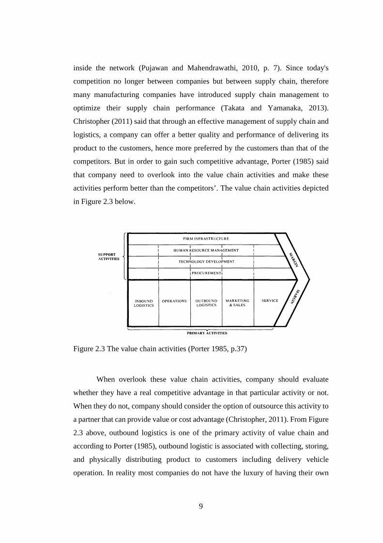
activities perform better than the competitors’. The value chain activities depicted
in Figure 2.3 below.
Figure 2.3 The value chain activities (Porter 1985, p.37)
When overlook these value chain activities, company should evaluate
whether they have a real competitive advantage in that particular activity or not.
When they do not, company should consider the option of outsource this activity to
a partner that can provide value or cost advantage (Christopher, 2011). From Figure
2.3 above, outbound logistics is one of the primary activity of value chain and
according to Porter (1985), outbound logistic is associated with collecting, storing,
and physically distributing product to customers including delivery vehicle
operation. In reality most companies do not have the luxury of having their own

10
fleet of vehicles and the drivers to perform physical distribution of the finished
products to the customer (or they could have but it would cost the company a lot of
funding). Hence, most of the companies outsource the finished goods delivery to
the trucking companies that would enable the value and cost advantage for the
company.
2.1.2. Supply Chain Vulnerability
The risk of disruption has been further exacerbated by recent trend and
practices in managing supply chain such increased complexity due to global
sourcing, increased reliance on outsourcing and partnering, single sourcing
strategies, and lean supply chain that focused on reducing inventory (Hendricks and
Singhal, 2005). Waters (2007) said that vulnerability reflects the likeliness of a
supply chain being disrupted. Furthermore, Jüttner (2005) found that managers
believed these trends/practices increased supply chain vulnerability: globalization
(52 percent of managers), reduction of inventory (51 percent), centralized
distribution (38%), supplier reduction (36 percent), outsourcing (30 percent), and
centralized production (29%).
2.1.3. The Role of Transportation in Supply Chain
Transportation refers to the movement of product from one location to
another as it makes its way from the beginning of a supply chain to the customer
(Chopra and Meindl, 2015). Transportation services play a central role in seamless
supply chain operations, moving inbound materials from supply sites to
manufacturing facilities, repositioning inventory among different plants and
distribution centers, and delivering finished products to customers (Stank and
Goldsby, 2000). Road transport has dominated the distribution of finished products
at the lower levels of the supply chain, particularly in the delivery of retail supplies
(McKinnon, 2006). By the recent adopted trends such lean supply chain, buffer
stocks have been severely reduced and with the customer’s demand of shorter order
lead times, making the finished goods distribution becomes highly sensitive to even

11
short delays in the transport system. Therefore, a low probability event such
disruption that temporarily halt the road freight system would have caused a severe
impact on the customer’s inventory level.
2.2. Supply Chain Disruption
Disruptions in supply chain defined by Wilson (2007) as unanticipated
event that interrupts the material flows in the supply chain, resulting in abrupt
cessation of the movement of the goods. Sources or drivers of these disruptions
stated by Chopra and Sodhi (2004) are natural disasters, labor dispute, supplier
bankruptcy, war and terrorism, and single source dependency. The nature of the
drivers described by Taleb (2007) as a black swan or Simchi-levi et al. (2008) as
unknown-unknown risk, an event that very unlikely to occurred but has massive
impact. The massive-negative impact was shown through a study conducted by
Hendricks and Singhal (2003), found that supply chain disruptions has caused
107% decrease in operating income, 7% lower sales growth, 11% higher costs, and
33 – 40 % lower stock returns after three years period of the disruption.
2.2.1. Transportation Disruption
Transportation disruption defined by Sheffi et al. (2003) as delay or
unavailability of the transportation infrastructure, leading to the impossibility to
move goods, either inbound and outbound. The uniqueness of transportation
disruption that differentiate it from supply disruption lies in the availability of the
both parties, consigner and consignee. Let us take a simple supply chain, consists
of one supplier one distributor. In the case of supply disruption, supplier is the one
that having disruption event, causing inability to supply material/products to the
unharmed distributor. In the case of transportation disruption, both supplier
(consigner) and distributor (consignee) are intact/unharmed because disruption only
occurred in the transportation infrastructure. An example of transportation
disruption occurred in real supply chain operations was the event of volcanic
eruption of mount Eyjafjallajökull in Iceland 2010. The eruption crippled the air
12
transportation within the area and cause negative impact on economy. Some of the
notable impacts were: (1) causing a grounded cargo shipment from Africa, made
Kenya’s farmers to dump tones of vegetables and flowers destined for the UK
causing financial loss of $1.3m a day (Wadhams, 2010); (2) causing interruptions
in the supply of parts that forced BMW to suspends production at three of its plants
in Germany which affecting 7000 vehicles and forced Nissan to stop productions
in two factories in Japan which affecting 2000 vehicles (Wearden, 2010).
Published research that studying phenomena of transportation disruption in
supply chain are as follows: Wilson (2007), Yang and Wu (2007), Bai and Wang,
(2008), and Houshyar et al. (2013) found that transportation disruption may lead to
drop in supply chain performance. In addition, Wilson (2007) found that
transportation disruption type-2 (occurred between supplier and distributor) is the
most severe type of transportation disruption. Chen and Zhang (2009) proposed a
dispatching vehicle policy that optimize vehicle capacity and dispatching time
along a route should a transportation disruption occurred. Figliozzi and Zhang,
(2010) found that disruption costs include lost sales, expediting costs, intangibles
such as loss of reputation, and financial impacts on companies’ cash flows are very
difficult to quantify even with full access to a company’s proprietary operational,
financial, and sales data. Husdal and Brathen (2010) found that industry and
business are the immediate sector that experience the severe impact of
transportation disruption since the first day after disruption occurred. Ishfaq (2012)
found that flexibility in transportation can provide opportunity to build resilience
concept into the supply chain. Hishamuddin et al. (2013) found that optimal
recovery schedule is highly dependent on the relationship between the backorder
cost and the lost sales cost parameters. Cui et al. (2016) found that their proposed
model can yield a supply chain system design that minimizes the impacts from
probabilistic disruptions and also leverages expedited shipments and inventory
management to balance tradeoffs between transportation and inventory costs. Zhen
et al. (2016) found that the backup transportation is very efficient to reduce the
profit loss, causing a less insurance coverage to be purchased in advance of
disruption; Liu et al. (2016) found that the improved model of grey neural networks
is a feasible prediction method for transportation disruption. From the literatures

13
mentioned above, we summarized 5 facts of transportation disruption as the
following:
1. By the case of BMW and Nissan (Wearden, 2010), transportation disruption
leads to supply disruption;
2. Based on the type of the goods flow, transportation disruption has the most
negative impact when occurred between manufacturer and distributor (type-2)
(Wilson, 2007);
3. In addition, during transportation disruption occurrence, distributor’s
(consignee) inventory level is exhaust or in a stockouts period, but when the
disruption finished, the inventory level extremely increased (Wilson, 2007);
4. By the case of BMW, Nissan, and Kenya’s flower industry, we concluded that
based on the product characteristics, transportation disruption has a great
negative impact on product with un-perishable (high value – low volume)
characteristics and perishable (low value – high volume) characteristics.
5. The more the transportation lead time, the greater the impact of transportation
disruption.
2.3. Responses Against Disruption
The drivers of supply chain disruption Chopra and Sodhi (2004), are
something that beyond a manager control and taking care of this problem will
always adding extra costs, disturbing the cost efficiency of the supply chain (Chopra
and Sodhi, 2014). Hence, dealing with disruption in supply chain left the manager
with three options, which are risk acceptance (do nothing), risk shifting (insurance),
and tailor mitigation strategies.
2.3.1. Risk Acceptance
The first option roots from the fact that most managers know the inherently
risky supply chain is, but chose to do nothing either to avoid the incurred extra costs
and/or don’t know how to proactively or reactively deal with the risk. Simchi-Levi
et al. (2015) found that managers choose to do nothing against the risk of
14
disruptions, not only because they are afraid to misallocate financial resources (i.e.
tailoring mitigation strategies) that might end up in a poor financial performance
report but also investing in such mitigation strategies would not giving them
spotlight whether or not an actual disruption occurred. Therefore, this option is
commonly adopted by the manager, but Chopra and Sodhi (2014) mentioned that
doing nothing will likely gave the most severe impact.
2.3.2. Risk Shifting
The second option arose because managers saw disruptions as something
that has extremely low probability of occurrence, hence insurance assumed to be
the best measurement to deal with it. Gurnani and Mehrotra (2012) noted that a
disruption event in one link could quickly ripple to another link in the chain. Using
the same logic, it is believed that a potential transportation disruption has ripple
effects both downstream and upstream (Wilson, 2007), therefore could ‘‘quickly
cripple the entire supply chain” (Giunipero and Eltantawy, 2004, p. 703). From this
fact, we argued that insurance policy is ineffective to cover the whole economic
impact caused by transportation disruption. This argument was strengthened by
several literatures. Stauffer (2003) in his report noted that trying to cover the risks
through insurance is no longer as feasible as it once was. Paulsson (2007) stated
that compensation from a third party (i.e. insurance company) for the negative
effects of a disruption rarely covers fully the negative effects seen from a supply
chain perspective. Gurnani and Mehrotra (2012) noted that if insurance is available,
it can only mitigate the direct impact (i.e. the loss of revenue), but it cannot replace
customers who impatiently turn to the competitors during a disruption, nor can it
restore a loss of reputation. Renesas (2011, p.16) in their report showed that
insurance only cover approximately 24% of the total 65.5-billion-yen economic
loss caused by the Great East Japan Earthquake in 2011. In global perspective,
Munich Re (2016, p.56) showed that in the event of disaster/catastrophic, insurance
policy only cover relatively small proportion compared to the overall economic
loss. Hence, Olson and Swenseth (2014) suggested that rather than relying on
simple insurance, it is better to rely on the broader view of risk management that
15
offers risks prevention or impact reduction, through loss-prevention and control
systems. In addition, we believed that relying on insurance to deal with
transportation disruptions in supply chain was also irrelevant, since disruption
occurred because of the unavailability of transportation infrastructures which fall
in local or central government responsibility which of course, outside the coverage
of insurance policy.
2.3.3. Risk Mitigation
There exist several strategies to deal with supply chain disruptions or
particularly, transportation disruption. Chopra and Sodhi (2004) proposed several
strategies to mitigate various risk in supply chain, from these strategies, we
identified that adding capacity, adding inventory, having redundant suppliers,
increasing responsiveness, increasing flexibility, and increasing capability were
strategies that suitable to mitigate disruption risk. Tang (2006) noted that
postponement, strategic stock, flexible supply base, make-and-buy, economic
incentives, flexible transportation, revenue management, dynamic assortment
planning, and silent product rollover were the robust strategies to mitigate supply
chain disruptions. Wilson (2007) proposed alternative routes, alternative modes of
transportation, alternative suppliers, transshipment strategic between warehouse,
VMI, carrying additional inventory, having redundant supplier, postponement, and
mass customization to protect against transportation disruption risk in supply chain.
Stecke and Kumar (2009) proposed several coping actions to mitigate the effect of
transportation disruption risk in supply chain that mainly in a form of flexibility and
redundancy, which were: maintain multiple manufacturing facilities with flexible
and/or redundant resources, carry extra inventory, secure alternate suppliers, choose
flexible transportation options, standardize and simplify process, component
commonality, postponement, influence customer choice, and insurance. Chen and
Ji (2009) proposed adopting less risky transportation mode and alternative
transportation modes to avoid transportation disruption risk, also outsource to 3PL
as effective way to reduce transportation disruption risk. Ishfaq (2012) was building
resilience into supply chain via transportation flexibility (routes and modes) in

16
response of transportation disruption events. Fan et al. (2016) build flexibility into
supply chain via postponement strategy to create slack time against supply chain
disruptions; this slack time existed as a result of diversified speed of transportation
modes.
This third option is aimed to build a resilient supply chain that able to
maintain its desired performance level even tough disruption occurred. As
mentioned by Sheffi et al. (2003) , creating a resilient supply chain commonly
through two approaches: building flexibility and redundancy. Furthermore, Sheffi
et al. (2003) stated that redundancy is easy to build and less expensive in short term,
while building flexibility is difficult and costly but appears to be more cost-effective
compared to building redundancy in long term. In addition, according to Pujawan
(2004), one should not pursuing high degree of flexibility unless the market
indicates the need for it. Furthermore, Rice and Caniato (2003) was also suggested
that it is possible for the company to adopt a combination of flexibility and
redundancy.
1. Redundancy
Redundancy requires the firm to maintain capacity to respond to disruptions in
the supply chain, largely through investments in capital and capacity prior to
the point of need (Rice and Caniato, 2003). Simchi-levi et al. (2008) proposed
an investment in redundancy to manage the risk of disruptions in supply chain.
A more detail application of redundancy as mitigation strategy against
disruptions was conducted by Son and Orchard (2013). They applied redundant
strategy to mitigate supply disruption by proposing Q-policy which add extra
quantity to initial the initial order of the EOQ and R-policy which build an
exclusive stock, preserved to protect the retailer/distributor from stockouts
during disruption period. They found that R-policy dominantly advantageous
than Q-policy.
2. Flexibility
Flexibility requires the firm to create capabilities in the firm’s organization to
respond against disruptions in supply chain by using existing capacity that can
be redirected or reallocated (Rice and Caniato, 2003). Ishfaq (2012)

17
investigated whether the existing US transportation networks provide an
opportunity to improve the resilience of a supply chain network through the
proposed flexible logistics strategy. The exploratory study showed that
companies can improve the resilience of their supply chains by maintaining
flexible transportation operations.
3. Combination of Flexibility and Redundancy
Rice and Caniato (2003) noted that firm will likely choose a mixture of
flexibility and redundancy by taking into consideration the different cost and
service characteristics offered by flexibility and redundancy. Schmitt (2011)
showed that a combined policy between inventory reserves and back-up
capabilities could give the best protection against supply chain disruption.
2.4. Simulation Modeling
Blanchard and Fabrycky (2006) defined system as a set of interconnected
components working together toward a common objective. A system could have so
many components that interconnected with unique behavior to each other, thus
increasing the system complexity. In order to provides performance measurement
of this complex system, an act of modeling is needed. Such a simplified
representation of an actual and complex system is called a model, hence, simulation
modeling is an attempt to analyze complex systems by a simplified representation
of a system under study (Altiok and Melamed, 2010). A main reason behind
conducting a simulation modeling is that it has the capability of modeling the
system and its complex interrelationships and at the same time enabling low cost
investigation to make conclusions about how the actual system might behave
(Rossetti, 2015). There exist several types of simulation model:
1. Static vs. Dynamic: it considered static if the system under investigation doesn’t
change significantly with respect of time, but if it changes with respect of time,
then it considered as dynamic.
2. Discrete vs. Continuous: If a simulation model dynamically changes at discrete
points in time then it considered as discrete simulation model. If the model

18
dynamically changes at continuously in time that it considered as continuous
simulation model.
3. Deterministic vs. Stochastic: a simulation model considered as deterministic if
the model doesn’t have random input. But if there is a least some input being
random then it considered as stochastic.
Besides the aforementioned types of simulation model, when running a
simulation model in a simulation software, the simulator should aware that there
are two types of time frame of simulation, named steady-state simulation and
terminating simulation. A steady-state simulation recognized by its nature that has
no clear point of time of which would terminate the simulation running, sometimes
the time frame itself theoretically infinite. In practice, a steady-state simulation will
be run in a very long time and terminated only if it reaches a steady-state condition.
In opposite, a terminating simulation recognized by a limited time frame which
dictated by the model itself. The beginning and the termination of the simulation
are clearly defined and reflect the natural behavior of how the system under study
works. Although Discrete-Event Simulation (DES) and Monte Carlo simulation
shows similarities in its practicality on discrete system behavior, we chose DES
instead of Monte Carlo simulation as the approach to simulate system under study
because in opposite with Monte Carlo, which is basically sampling experiments and
time independent (Olson and Evans, 2002), the system under study involve the time
path and an explicit representation of the sequence in which events occur. In
comparison with the previous research, particularly by Wilson (2007) and Yang
and Wu (2007), this research decided to choose DES instead of system dynamic
(SD) because in opposite with SD, which objective is more on the strategic level in
order to gain insight into the interrelations between the different parts of a complex
system (Brailsford and Hilton, 2001), the objective of this research was to compare
and evaluate alternate strategies in tactical /operational decision making level, of
which strongly lead this research towards the characteristics of DES as described
by Brailsford and Hilton (2001) and Tako and Robinson (2009).

19
2.4.1. Application of Simulation in Risk Management
Simulation has been widely used as a tool in risk management, particularly
within supply chain disruptions. Schmitt and Singh (2009) used Monte Carlo
simulation to assess the vulnerability of supply chain against disruption risk and
quantity the impact on customer service. Son and Orchard (2013) Measured the
effectiveness of two mitigation strategy: reserved stock (R-policy) and larger order
quantity (Q-policy) using simulation. They found that R-policy had better
performance that Q-policy. In transportation disruption, simulation also had been
proven as a valuable tool. Wilson (2007) used simulation to measure the impact of
transportation disruption in supply chain performance. Yang and Wu (2007) also
used simulation to investigate the impact of transportation disruption on
performance of e-collaboration supply chain. Bai and Wang (2008) applied
discrete-continuous combined simulation to simulate supply chain under
transportation disruption using VMI and traditional structure. Pujawan et al. (2015)
demonstrated that, by using simulation modelling, the impracticality and difficulty
of analytical methods especially when the system exhibits uncertainties and
incorporates stochastic variables can be overcome.
2.4.2. Conducting Simulation Study
There exist several literatures that proposed a good guidance to conduct a
simulation study, such Banks (1998), Law (2007) , Sadowski (2007), and Rossetti
(2015) . We chose to use guidance from Banks (1998), since his methodology was
used as the main reference by Law (2007) , Sadowski (2007), and Rossetti (2015).
Banks (1998) proposed 12 steps in simulation which depicted in Figure 2.4. Each
step in Figure 2.4 was also presented in simulation methodologies that proposed by
the other literatures either in the same terms or different. The sequence of
undergoing each step was also similar. Below are brief explanations of each step:
1. Problem formulation. This should be the first step taken by the analyst since
this will determine the direction of simulation study. Therefore, problem
formulation need to be set and stated clearly, either by the analyst itself or by

20
Figure 2.4 12 Steps in simulation study (Banks, 1998, p. 16)
Problem Formulation
Setting of objectives and overall project plan
Model conceptualization Data collection
Model translation
Verified?
Validated?
Experimental design
Production runs and analysis
More runs?
Documentation and reporting
Implementation
Yes
No
No No
No
Yes
Yes

21
the client (decision maker). Along the progression of the simulation study,
sometimes this step need to be revisited or harnessed.
2. Setting of objectives. This step should set a detailed description of the objective
of the study which often includes general goals such comparison, optimization,
prediction, and investigation (Rossetti, 2015). The objectives indicate the
questions to be answered by simulation study based on the problem formulation
(Banks, 1998).
3. Model conceptualization. In this step, the analyst tried to abstracting the real-
world system under study by building mathematical and logical relationship
concerning the structure of the system (Banks, 1998). The purpose of
conceptual modeling tools is to convey a more detailed system description so
that the model may be translated into a computer representation (Rossetti,
2015).
4. Data collection usually takes a large portion of time required to perform
simulation study, therefore it is wise to begin this step as early as possible,
simultaneously with model conceptualization (Banks et al., 2010). This also
indicates that the analyst can readily construct the model while the data
collection is progressing (Banks, 1998)
5. Model translation can begin immediately after the model conceptualization and
data collection completed. Model translation is coding the conceptual model
into a computerized model (Banks, 1998). After computerized model complete,
it is ready to be operationalized by deploying the data collected into the
computerized model. This first operationalization called pilot run with only 1
replication.
6. Verification concerns with the issue of whether the computerized model is
working as it should. Verification is making sure that the computerized model
doesn’t deviate from its conceptual model. The accuracy of transforming a
problem formulation into a conceptual model or the accuracy of converting a
conceptual model into an executable computerized model is evaluated in model
verification (Balci, 2002).
7. Validation concerns with the issue of whether the conceptual simulation model
is an accuracy rate representation of the real system / system under study

22
(Banks, 1998; Kleijnen, 1995a). If there is an existing real system, then it is
advisable to compare the simulation output with the existing system to perform
a model validation. But, there are cases that the system under study is not exist,
for example when the purpose of the simulation study is to propose a new design
of a system. Approaches or techniques to perform model verification and
validation (V&V) were mentioned and explained in the literature by Balci
(1994, p.154), Kleijnen (1995b), Banks (1998, p.23), Law (2007, p.253),
Sargent (2013, p.16).
8. When the computerized model which operationalized in the pilot run passed the
V&V process, then this step decides to determine which factors have the
greatest effect on a response which is often called factor screening or sensitivity
analysis (Law, 2007)
9. In this step, the initial run (which was only 1 replication) then advanced to the
production run with more than 1 replication. The outputs from production run
then analyzed to measure the performance for the system being simulated. This
analysis process was referred by Sadowski (2007, p.273) and Law (2015) as
statistical analysis of simulation output to determine the accuracy of the output.
10. When the accuracy is below the predetermined desirable level, adjustments are
needed. The analyst determines whether additional runs are needed or if
additional scenarios need to be simulated (Banks, 1998).
11. Documentation and reporting serve numerous reasons such giving the
opportunity for the same or different analyst to understand how the simulation
model operates, stimulate confidence of the simulation model by the client, and
enable the client to easily review the final recommendation from the analyst
(Banks, 1998).
12. The successful of implementation depends on how well the previous 11 steps
have been performed (Banks et al., 2010).
In summary, these 12 steps of simulation study can represent in 4 major
phases. The first phase consists of step 1 and 2 is called the clarifications and
recalibrations phase. Because this phase entails the analyst or the client to clarify
the problems and objectives that the simulation model tries to address. Also because
23
sometimes analyst and client need to recalibrate these problems and objectives as
the simulation progressing. The second phase consists of step 3, 4, 5, 6, and 7, which
is the actual model building and data collection. Therefore, in the progress
sometimes a continuing interplay among steps is required (Banks et al., 2010). The
third phase consists of phase 8, 9, and 10, that concerns with running and
experimenting the simulation model to produce the early specified of desirable
output. The output variables then analyzed to estimate a contained random error by
using proper statistical analysis (Banks et al., 2010). The fourth phase called
implementation, contains step 11 and 12. The success of implementation depends
on how well the previous 11 steps have been performed (Banks et al., 2010).
2.5. Cost-Effectiveness Analysis (CEA)
As stated by Karlsson and Johannesson (1996), CEA is based on the
maximization of the health effects for a given amount of resources. Therefore, CEA
as decision making tool is used commonly in the field of medicine and health care,
for example: measuring the cost per effectiveness of various prescribed drugs or the
cost per quality gained of various given treatments. Incorporating the concept of
CEA into the second objective of this research, made us basing the CEA on the
minimization of negative effects of transportation disruption for a certain amount
of consequential costs. There are always 2 inputs in CEA, where the costs are
measured in monetary units and the effects are measured in non-monetary units
(Karlsson and Johannesson, 1996). CEA is preferred over cost-benefit analysis
(CBA) when monetizing all the benefit of the proposed alternative of strategies is
difficult (Boardman et al., 2010). Gift and Marrazzo (2007) showed that CEA
strengths lie on its ability to express cost per unit outcome and allows for
comparison of different interventions that achieving the same outcome; while weak
because unable to compare different interventions that producing different
outcomes. They also showed that CBA strengths lie in its ability to express all costs
and outcomes in monetary terms and allow for different interventions; while having
weakness because dictating expression of welfare effects in monetary terms, which

24
can be difficult and may not be widely accepted. In addition, we summarized
decision rules of CEA as follows:
1. A proper CEA is always comparative in nature (Petitti, 1999). When using
CEA, one should know that there is more than one strategy to be evaluated and
each strategy is competing with each other;
2. All of the evaluated strategies should assumed to be mutually exclusive
(Karlsson and Johannesson, 1996). Therefore, decision maker can only
execute/implement one strategy while neglecting the other (one can choose A
or B, but not both);
3. Since its competing and mutually exclusive nature, it is impossible to conclude
anything (what strategy to be implemented) about the cost effectiveness of the
different strategies based on average cost-effectiveness ratios, instead, one is
dictated to conduct CEA using incremental cost-effectiveness ratio (ICER)
(Karlsson and Johannesson, 1996);
4. Because of its mutually exclusive nature, cost-effectiveness ratio cannot be
interpreted as a rank list (Johannesson and Weinstein, 1993);
5. Comparing between cost-effectiveness ratio of each strategy can only be made
between strategy that producing the same outcome (Johannesson and
Weinstein, 1993).
Talluri et al. (2013) highlighted the importance of testing and comparing
alternative mitigation strategies in a comprehensive manner against a particular
type of risk. The fundamental nature of CEA that centered on the comparative and
mutually exclusive behavior; the advantage of CEA over CBA, of which doesn’t
entail any monetization of performance given by each mitigation strategy; and the
non-financial performance measurement that we used as our effectiveness input,
were 3 particulars that provided us with a plausible argument to choose CEA for
testing and comparing our proposed mitigation strategies against transportation
disruption.

25
2.5.1. Incremental Cost-Effectiveness Ratio (ICER)
While an average cost-effectiveness ratio (ACER) is estimated by dividing
the consequential cost of a strategy by a measure of effectiveness without any
concern to its alternatives, an incremental or marginal cost-effectiveness ratio
(ICER) is an estimate of the cost per unit of effectiveness of switching from one
strategy to another, or the cost of using one strategy in preference to another (Petitti,
1999). ICER mathematically expressed in Equation 2.1 below.
𝐼𝐼𝐼𝐼𝐼𝐼𝐼𝐼(𝑖𝑖) = 𝐶𝐶𝐶𝐶𝐶𝐶𝐶𝐶 (𝑖𝑖) − 𝐶𝐶𝐶𝐶𝐶𝐶𝐶𝐶 ( 𝑖𝑖−1)
𝐸𝐸𝐸𝐸𝐸𝐸𝐸𝐸𝐸𝐸𝐶𝐶𝑖𝑖𝐸𝐸𝐸𝐸𝐸𝐸𝐸𝐸𝐶𝐶𝐶𝐶 (𝑖𝑖)− 𝐸𝐸𝐸𝐸𝐸𝐸𝐸𝐸𝐸𝐸𝐶𝐶𝑖𝑖𝐸𝐸𝐸𝐸𝐸𝐸𝐸𝐸𝐶𝐶𝐶𝐶 (𝑖𝑖−1) (2.1)
where:
𝐼𝐼𝐼𝐼𝐼𝐼𝐼𝐼(𝑖𝑖) = the cost-effectiveness ratio when switching strategy (𝑖𝑖 − 1) with
𝑖𝑖
subscript 𝑖𝑖 = strategy 𝑖𝑖 ; 𝑖𝑖 = 2, 3, …, 𝐼𝐼
𝐼𝐼 = number of proposed strategies
Since this research concerns with evaluating 4 strategies that compete each
other in response to transportation disruption, where decision maker has limited
amount of fund (therefore can only implement one strategy), it is clear that ICER is
an obvious choice. According to Petitti (1999), before the cost is valued,
contributors of the cost should be defined first. One of the cost contributors that
Petitti (1999) introduced that relevant with this research is direct costs, which we
interpreted as monetary value consumed due to implementing a strategy.
Effectiveness in the other hand not measured in monetary value. In correlation with
transportation disruption, we used the same measurement of Wilson (2007) which
is unfilled customer orders as our degree of effectiveness.
An effective algorithm to correctly calculate ICER has been introduced by
Johannesson and Weinstein (1993) and conducted via a hypothetical case by
(Karlsson and Johannesson (1996). We summarized this efficient algorithm as
follows:
1. Define cost and effectiveness terms are referring to;

26
2. Measure/calculate the cost and effectiveness for each strategy;
3. List strategies in ascending order of either effectiveness or costs;
4. Identify and eliminate strongly dominated strategy (have increased costs and
reduced effectiveness compared with the immediate alternative) and/or;
5. Identify and eliminate weakly dominated strategy (have equal cost with reduced
effectiveness or increased costs with same effectiveness compared with the
immediate alternative);
6. Calculate ICER using Equation 2.1.
7. If ICERi ˃ ICERi+1 (ICER changed in descending order) then strategy 𝑖𝑖
considered to be extended dominated by strategy 𝑖𝑖 + 1, thus should be
eliminated.
8. Repeat step 6 and 7 if necessary
9. Produce recommendation of acceptable strategy based on the ICERs
When 𝑖𝑖 = 1, this strategy is called the base case which refers to the current
or typical deployed strategy. Consistently with Equation 2.1, base case is
automatically skipped in step 6. Strongly dominated in step 4 means that strategy 𝑖𝑖
is less cost-effective than strategy 𝑖𝑖 + 1, since strategy 𝑖𝑖+1 gives lesser cost with
better effectiveness. Weakly dominated in step 5 means that strategy 𝑖𝑖 is less cost-
effective than strategy 𝑖𝑖 + 1 since strategy 𝑖𝑖 + 1 either gives same cost with better
effectiveness or lesser cost with same effectiveness. Extended dominated in step 7
means that strategy 𝑖𝑖 is less effective than strategy 𝑖𝑖 + 1, since switching directly
from strategy 𝑖𝑖 − 1 to strategy 𝑖𝑖 + 1 gives better effectiveness with lesser cost than
switching from strategy 𝑖𝑖 to strategy 𝑖𝑖 + 1 which gives lesser effectiveness with
greater cost.
2.5.2. Application of Cost-Effectiveness in Risk Management
In risk management, cost-effectiveness was used by Schmit and Roth (1990)
to evaluate the effectiveness of various risk management practices. Sherwin et al.
(2016) also evaluated cost-effectiveness of mitigation strategies with a low volume
high value supply chain against delay risk due to unreliable production process.
27
2.6. Research Gap
Table 2.1 below shows previous research of transportation disruption and
position of this research relative to those previous research. To the best of our
knowledge, a research by Wilson (2007) was the initial focused research in
transportation disruption. Furthermore, it was mentioned by Ho et al. (2015), that
transportation disruption in contrast to supply disruption, has received little
attention by academic. The first gap we’d like to address in this research is the lack
of contribution on the transportation disruption knowledge.
From Table 2.1 below, we could also realize that there are 6 papers that
fused strategies and investigates SC performance under transportation disruption
event. But from this 6 papers, only the paper by Ishfaq (2012) that used case study
as data source for the investigation, the other 5 papers used numerical example.
The second gap we’d like to address in this research is the lack of case study as data
source on investigation of SC performance under transportation disruption event.
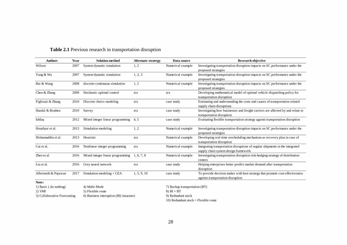
28
Table 2.1 Previous research in transportation disruption
Authors Year Solution method Alternate strategy Data source Research objectiveWilson 2007 System dynamic simulation 1, 2 Numerical example
Yang & Wu 2007 System dynamic simulation 1, 2, 3 Numerical example
Bai & Wang 2008 discrete-continuous simulation 1, 2 Numerical example
Chen & Zhang 2009 Stochastic optimal control n/a n/a
Figliozzi & Zhang 2010 Discrete choice modeling n/a case study
Husdal & Brathen 2010 Survey n/a case study
Ishfaq 2012 Mixed integer linear programming 4, 5 case study
Houshyar et al. 2013 Simulation modeling 1, 2 Numerical example
Hishamuddin et al. 2013 Heuristic n/a Numerical example
Cui et al. 2016 Nonlinear integer programming n/a Numerical example
Zhen et al. 2016 Mixed integer linear programming 1, 6, 7, 8 Numerical example
Liu et al. 2016 Grey neural network n/a case study
Albertzeth & Pujawan 2017 Simulation modeling + CEA 1, 5, 9, 10 case study
Note:1) Basic ( do nothing) 4) Multi-Mode 7) Backup transportation (BT)2) VMI 5) Flexible route 8) BI + BT3) Collaborative Forecasting 6) Business interuption (BI) insurance 9) Redundant stock
10) Redundant stock + Flexible route
Investigating transportation disruption risk-hedging strategy of distribution centersHelping enterprises better predict market demand after transportation disruptionTo provide decision maker with best strategy that promote cost-effectiveness against transportation disruption
Estimating and understanding the costs and causes of transportation related supply chain disruptionsInvestigating how businesses and freight carriers are affected by and relate to transportation disruptionEvaluating flexible transportation strategy against transportation disruption
Investigating transportation disruption impacts on SC performance under the proposed strategiesDeveloping real-time rescheduling mechanism as recovery plan in case of transportation disruption
Investigating transportation disruption impacts on SC performance under the proposed strategiesInvestigating transportation disruption impacts on SC performance under the proposed strategiesInvestigating transportation disruption impacts on SC performance under the proposed strategiesDeveloping mathematical model of optimal vehicle dispatching policy for transportation disruption
Integrating transportation disruptions of regular shipments in the integrated supply chain system design framework

29
CHAPTER 3
RESEARCH METHODS
This chapter gives explanation about how we fulfill the objective of this
research by our constructed research framework. This chapter also shows methods
that we used in this research.
3.1. Research Framework
In Chapter 1 we specified a research questions (RQ) that we need to answer
in order to fulfill the objective of this research. This RQ laid a foundation of two
major constructs that builds our research framework, shown in Figure 3.1 below.
Figure 3.1 Research Framework
As shown by Figure 3.1 above, by using simulation modeling as a tool we
conducting a simulation study that would be able to obtain the cost and
effectiveness for each of the proposed strategy and by using CEA as our decision
analysis tool we would be able to measure their cost-effectiveness. This process
was executed sequentially since to conduct CEA, first we need to conduct
simulation study and use its outputs as our inputs to be fed into CEA. Feeding these
inputs into CEA will consequently assess the cost-effectiveness of which the output
will be the objective of this research.
Simulation Modeling CEA
Research Objective
Company’s data Input Ouput/Input Output

30
3.2. Methods on Simulation Modeling
The first construct of the research framework is shown in Figure 3.2 below.
This first construct shows that we used company’s data as an input to our
constructed model of system under study. Our model then simulate this input to
produce outputs that shall be used as an input of the second construct. While
simulation modeling is a tool, an act of conducting the simulation is called
simulation study.
Figure 3.2 First construct of the research framework
In Chapter 2, we had introduced a 12-steps of conducting simulation study
(depicting in Figure 2.4) by Banks (1998) also the arguments of why this steps are
adopted into this research. In the following sections we present the methods that we
used for these steps. But take notice that not every step needs specific method to be
able to be executed. For example, problem formulation (step 1) is quite easily
deduced and executed without needing any specific or scientific method. Therefore,
here we present the methods for data collection (step 4), model translation (step 5),
verification (step 6) and validation (step 7), experimental design (step 8),
production run and analysis (step 9), and more runs (step 10).
Simulation Modeling
Company’s data Input Ouput/Input
31
3.2.1. Data collection
Relating the methods for simulation input from Banks (1998) and (Law,
2007), we present 4 methods to convert the collected data from focal company into
a simulation input as follows:
1. Use directly the data values obtained as an input in the simulation. Hence, when
a simulation study use this method it’s called trace-driven simulation (Law,
2007, p. 279);
2. Fit a probability distribution to the data values. If there are sufficient data values,
say 50 or more it may be appropriate to fit a probability distribution to the data
(Banks, 1998, p. 20) using standard technique of statistical inference and perform
hypothesis test to determine the goodness of fit (Law, 2007, p. 279).
3. When it is not possible to fit the data into a probability distribution or the
suggested probability distributions found to be inconclusive (Banks, 1998, p.
21), the data values themselves are used to define an empirical distribution
function (Law, 2007, p. 279).
4. In a rare case when there are no data values are available, analyst may obtain a
subjective estimate or called guesstimate concerning the system under study
(Banks, 1998, p. 21).
3.2.2. Model translation
Model translation is coding the conceptual model into a computerized
model (Banks, 1998), but not ready to operationalized until the data collected
deployed into the computerized model. In order to coding the conceptual model into
computerized model, Law (2007, p. 188) presented 2 methods as the following:
1. Via programming languages: C, C++, or Java
2. Via simulation packages, which is divided into general purpose (i.e. Rockwell
Arena® and Extend ®) and application oriented (i.e. Flexim®, ProModel®, and
Quest®)
We decided to use Rockwell Arena® as our software package due to its
familiarity and simplicity that the software offered.

32
3.2.3. Verification and Validation (V&V)
Verification concerns with the issue of whether the computerized model is
working as it should while validation concerns with the issue of whether the
conceptual simulation model is an accuracy rate representation of the real system /
system under study (Banks, 1998; Kleijnen, 1995a). Approaches or techniques to
perform model V&V were mentioned and explained in the literature by Balci (1994,
p.154), Kleijnen (1995b), Banks (1998, p.23), Law (2007, p.253), Sargent (2013,
p.16). Here we listed methods of conducting verification from Law (2007) and
Banks (1998, p.23) as the following:
1. Law (2007): (1) program debug; (2) structured walk-through; (3) sensitivity
analysis; (4) compare with hand calculations (trace); (5) comparing the
simulation and analytic results from the simple case; (6) observe animation; (7)
compare mean and sample variance between simulation results and system
under study (historical data).
2. Banks (1998, p.23): (1) follow the principles of structured programming; (2)
make the operation model as self-documenting as possible; (3) have the
computer code checked by more than one person; (4) check to see that the
values of the input data are being used appropriately; (5) for a variety of input-
data values, ensure that the outputs are reasonable; (6) use the debugger feature;
(7) animation.
Here we listed methods of conducting validation from Law (2007) and
Sargent (2013, p.16) as the following:
1. Law (2007): (1) comparison with an existing system; (2) comparison with
another model; (3) comparison with expert opinion (face validity); (4) observe
animation; (5) inspection approach; (6) sensitivity analysis.
2. Sargent (2013, p.16): (1) face validity; (2) parameter variability–sensitivity
analysis; (3) extreme condition tests; (4) Turing test; (5) historical data
validation; (6) comparison to other model; (7) animation.

33
3.2.4. Experimental Design
In experimental design terminology, the input parameters and structural
assumptions composing a model are called factors, and output performance
measures are called responses. The major goal of experimental design in simulation
is to determine which factors have the greatest effect on a response which is often
called factor screening or sensitivity analysis (Law, 2007). Factors can be either
quantitative or qualitative and being controllable or uncontrollable. In experimental
design we usually focus on the quantitative factors which controllable. In
conducting experimental design instead of using one-factor-at-a time (OFAT), Law
(2007) advised to use factorial designs as our method since factorial designs is more
efficient and show us interactions. Factorial designs either be 2k Factorial Designs
or 2k-p Fractional Factorial Designs, depends on the number of factor 𝑘𝑘. Factors are
selected by analyst no more than 15, through intuition, prior knowledge, and the
like (Banks, 1998, p. 177).
3.2.5. Production Runs and Analysis
Production runs is simply change the number of replication which was only
1 in pilot run to be multiple run. In this research production run is done in 10
replications. After production runs is finished, Sadowski (2007, p.273) and Law
(2015) suggested that the output will be analyzed to measure its accuracy using a
method called the statistical analysis of simulation output. The statistical analysis
of simulation output was based on 3 classic statistical equations specified by Law
(2015, p. 1812). These 3 classic statistical equations are included in simulation
software package. For example, in Arena® these equations are already calculated
in the report under the term of half-width which represents the accuracy of the
reported simulation output.
3.2.6. More Runs
When the accuracy is below the predetermined desirable level, analyst
required to increase the accuracy, one suggested way by running more replications.

34
To determine how many replications are needed to correct the accuracy, Sadowski
(2007) proposed a method as expressed in Equation 3.1 below:
𝑛𝑛 ≅ 𝑛𝑛0ℎ02
ℎ2 (3.1)
where:
𝑛𝑛 = the new number of replications
𝑛𝑛0 = the number of initial replications
ℎ02 = the initial value of half-width
ℎ2 = the desired value of half-width
Calculating Equation 3.1 will result in an approximation of the number of
new replications that needed to be re-run into the simulation software. In summary,
combined all the methods mentioned above, we modified steps of simulation study
by (Banks, 1998) and presented the methods used to conduct simulation study as
depicted in Figure 3.3 below.

35
Problem Formulation
Setting objectives
Model conceptualization
Simulation inputs formulation
Computerize model in ARENA
Verified?
Validated?
Sensitivity analysis using factorial designs
Production run and output analysis
More replications?
Document cost and effectiveness
Conduct CEA
Yes
No
No No
No
Equation 3.1Yes
Figure 3.3 Methods to conduct simulation study for this research (adapted from
Banks (1998))

36
3.3. Methods on CEA
The second construct of the research framework was trying to assess the
cost-effectiveness of each strategy. This second construct as depicted in Figure 3.3
below can only be executed if the previous construct already gives outputs that will
be used as inputs to conduct CEA.
Figure 3.4 Second construct of the research framework
As shown in Figure 3.4 above, after conducting the CEA we can assess the
cost-effectiveness of each strategy and the output of this construct is a full operation
the research framework which fulfilled the objective of this research. As explained
in Chapter 2.5, due to its competitive and mutually exclusive nature of CEA, then
the essential of CEA lays on the calculation of ICER. We expressed the effective
algorithm of calculating ICER as the following:
1. Define cost and effectiveness terms are referring to;
2. Measure/calculate the cost and effectiveness for each strategy;
3. List strategies in ascending order of either effectiveness or costs;
4. Identify and eliminate strongly dominated strategy (have increased costs and
reduced effectiveness compared with the immediate alternative) and/or;
CEAResearch ObjectiveOuput/Input Output

37
5. Identify and eliminate weakly dominated strategy (have equal cost with reduced
effectiveness or increased costs with same effectiveness compared with the
immediate alternative);
6. Calculate ICER using Equation 2.1.
7. If ICERi ˃ ICERi+1 (ICER changed in descending order) then strategy 𝑖𝑖
considered to be extended dominated by strategy 𝑖𝑖 + 1, thus should be
eliminated.
8. Repeat step 6 and 7 if necessary
9. Produce recommendation of acceptable strategy based on the ICERs
Step 1 & 2 of the algorithm can be obtained from the output of simulation
study and that’s the reason why we could not conduct CEA before the simulation
study. We also added sensitivity analysis into the algorithm. Sensitivity analysis in
CEA served a quite similar purposes sensitivity analysis are mentioned as follows:
1. To find out how sensitive our cost-effectiveness ratios if factors changes;
2. To find out the robustness of the cost-effectiveness ratios if factor changes.
This CEA sensitivity analysis (CEA-SA) corresponded with the factors
changes in simulation study sensitivity analysis (SS-SA). In summary, we present
translate the effective algorithm of ICER in flowchart and use it as our method of
conducting CEA in Figure 3.5 below.

38
Figure 3.5 ICER effective algorithm as method to conduct CEA
List strategies in ascending order
Identify weakly and/or strongly dominated strategy
Dominated? Eliminate strategyYES
Calculate ICER
Identify extended dominated strategy
Dominated? Eliminate strategy
NO
YES
Sensitivity analysis
NO
END
Document final cost-effectiveness ratios
Introduce initial cost-effectiveness ratios
Obtain cost and effectiveness from simulation study

39
CHAPTER 4
DATA COLLECTION
This chapter describes about how we obtain the data for this research. This
includes the reasons for selecting the focal company (consigner) and the distributor
(consignee), consequent cost functions, delivery schedules, and natural disaster
frequency, transportation activity, and proposed strategies.
4.1 Relationship Between Focal Company and Distributor
Focal company (FC) located in Makassar City, South Sulawesi. FC’s main
product is wheat flour with more than 10 products with various brands in various
size (weight). FC’s market area divided into 3 regions, named local, east, and west.
Local area means that FC served only customers located in Makassar City. East
area means that FC served customers located outside Makassar City (Sulawesi
Island), East Java, Kalimantan, and Indonesia’s east region. West area covers the
rest. In distributing its finished products, FC used 2 transportation modes of water
(vessel) and land (truck). FC outsource this transportation activity to the 3rd party.
For the local area, all transportation handled by using trucks and for the west area,
transportation handled using vessel to the port and trucks from port to warehouses.
For the east area some customers (medium distance) were still served using trucks
(i.e. Tana Toraja, Poso, and Luwuk) and some customers (longer distance) were
served by vessel (i.e. Kendari, Gorontalo, and Papua). We chose this FC because
the perishability of the finished products (which highly rejected by customers if
more than 2 weeks old stored and the commitment of FC to maintain an excellent
service level to its customers with lowest costs (as noted in the FC’s vision and
mission).
We then chose a sole distributor in Poso City, Central Sulawesi. There is no
other distributor that partnering with FC in Poso. We chose this distributor because
it has the longest lead time (here assumed equal to distance) from FC’s location and
its delivery is still served by trucks. The delivery activity between FC and
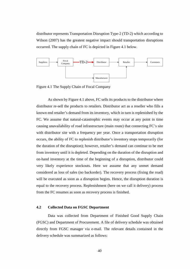
40
distributor represents Transportation Disruption Type-2 (TD-2) which according to
Wilson (2007) has the greatest negative impact should transportation disruptions
occurred. The supply chain of FC is depicted in Figure 4.1 below.
Figure 4.1 The Supply Chain of Focal Company
As shown by Figure 4.1 above, FC sells its products to the distributor where
distributor re-sell the products to retailers. Distributor act as a reseller who fills a
known end retailer’s demand from its inventory, which in turn is replenished by the
FC. We assume that natural-catastrophic events may occur at any point in time
causing unavailability of road infrastructure (main route) that connecting FC’s site
with distributor site with a frequency per year. Once a transportation disruption
occurs, the ability of FC to replenish distributor’s inventory stops temporarily (for
the duration of the disruption); however, retailer’s demand can continue to be met
from inventory until it is depleted. Depending on the duration of the disruption and
on-hand inventory at the time of the beginning of a disruption, distributor could
very likely experience stockouts. Here we assume that any unmet demand
considered as loss of sales (no backorder). The recovery process (fixing the road)
will be executed as soon as a disruption begins. Hence, the disruption duration is
equal to the recovery process. Replenishment (here on we call it delivery) process
from the FC resumes as soon as recovery process is finished.
4.2 Collected Data on FGSC Department
Data was collected from Department of Finished Good Supply Chain
(FGSC) and Department of Procurement. A file of delivery schedule was obtained
directly from FGSC manager via e-mail. The relevant details contained in the
delivery schedule was summarized as follows:
Suppliers Focal Company Distributor Retailer Customers
Manufacturer
TD-2

41
1. Delivery history: January 2016 - December 2016
This was the first obstacle during data collection process. FC was adopting and
using Microsoft Dynamics AX as their ERP software since 2012. Even tough
distributor has established business with FC more than 20 years, the historical
data recorded digitally was started from 2012 record. In addition, when the
Manager of FGSC department tried to ‘pull’ the records, the oldest historical
data stored in the server was from the year of 2016 above. We tried to check
another customer served by truck (i.e. Palopo, Luwuk, Tana Toraja) but the
result stayed the same. We concluded that since the delivery data records of
trucking-served customers are vast, then the IT department must be set the
system to remove data that more than 2 years old. That is why the oldest data
in the server starts from 2016. This fact has consequence to determine
simulation input in ARENA.
2. Delivery Date:
This is the actual date of delivery from FC in Makassar to distributor’s site in
Poso. Actual delivery date shows the exact date of trucks leaving FC’s site for
delivering products to distributor.
3. Customer’s Order (CO) date:
This is a recorded date of distributor asking (placing order) FC to deliver certain
product brand in certain quantity to its site.
4. Brands, Quantity, and Volume:
Data of brands and its quantity that delivered to distributor’s site. Brands,
quantity, and volume determined by the customer’s order. Volume is measured
in metric ton (MT). There were 15 brands delivered during year of 2016. These
15 brands were delivered in different quantity and each brand has certain SKU.
For the sake of simplicity, we would choose brands that represent 80% of total
volume delivered and we found that brand A, B, C, D, and E were representing.
These 5 selected brands together with the other 10 were presented in Table 4.1
below.

42
Table 4.1 Delivered brands during the year of 2016
Continuing data in Table 4.1, we also show the delivery details for brand A,
B, C, D, and E consecutively in Table 4.2, Table 4.3, Table 4.4, Table 4.5, and
Table 4.6.
Table 4.2 Delivery details for brand A
Brand SKU (Kg) Qty Total Volume (Kg)A 25 9695 242375B 10 14856 148560C 25 5430 135750D 25 4506 112650E 25 3754 93850F 25 900 22500G 20 1102 22040H 25 500 12500I 9 1100 9900J 10 900 9000K 10 900 9000L 20 300 6000M 10 250 2500N 1.8 498 896.4
827521.4Total
Date of Delivery Days in Year Qty (Zak) MT1/26/2016 25 780.00 19.52/22/2016 52 100.00 2.52/23/2016 53 400.00 103/12/2016 71 300.00 7.53/31/2016 90 300.00 7.54/11/2016 101 1000.00 254/19/2016 109 600.00 154/30/2016 120 800.00 205/12/2016 132 1000.00 255/21/2016 141 600.00 155/25/2016 145 600.00 155/26/2016 146 1000.00 255/27/2016 147 800.00 206/3/2016 154 400.00 10
6/14/2016 165 200.00 56/27/2016 178 300.00 7.57/26/2016 207 515.00 12.875

43
Table. 4.3 Delivery details for brand B
Table. 4.4 Delivery details for brand C
Date of Delivery Days in Year Qty (Box) MT1/26/2016 25 300.00 32/22/2016 52 200.00 23/12/2016 71 750.00 7.53/31/2016 90 500.00 54/11/2016 101 2000.00 204/19/2016 109 1000.00 105/27/2016 147 1000.00 106/3/2016 154 1000.00 10
6/14/2016 165 1000.00 106/27/2016 178 1000.00 107/26/2016 207 800.00 89/26/2016 269 2100.00 219/27/2016 270 1000.00 10
10/22/2016 295 750.00 7.510/24/2016 297 750.00 7.511/9/2016 313 400.00 4
12/30/2016 364 306.00 3.06
Date of Delivery Days in Year Qty (Zak) MT1/26/2016 25 500.00 12.52/22/2016 52 1,000.00 254/30/2016 120 200.00 55/21/2016 141 300.00 7.55/25/2016 145 200.00 55/27/2016 147 500 12.56/20/2016 171 1000 256/23/2016 174 1000 256/27/2016 178 200 57/26/2016 207 530 13.25

44
Table. 4.5 Delivery details for brand D
Table. 4.6 Delivery details for brand E
Date of Delivery Days in Year Qty (Zak) MT1/26/2016 25 100.00 2.52/22/2016 52 100.00 2.53/11/2016 70 600.00 155/21/2016 141 100.00 2.55/25/2016 145 100.00 2.56/3/2016 154 200 5
6/14/2016 165 300 7.57/26/2016 207 400 108/9/2016 221 500 12.5
9/26/2016 269 300 7.59/27/2016 270 300 7.5
10/22/2016 295 300 7.510/24/2016 297 300 7.511/9/2016 313 300 7.5
11/25/2016 329 300 7.512/30/2016 364 306 7.65
Date of Delivery Days in Year Qty (Zak) MT1/26/2016 25 100 2.52/23/2016 53 200 53/11/2016 70 400 103/12/2016 71 200 53/31/2016 90 350 8.754/11/2016 101 200 55/25/2016 145 100 2.55/27/2016 147 100 2.56/14/2016 165 100 2.56/27/2016 178 100 2.57/26/2016 207 200 58/9/2016 221 300 7.5
9/26/2016 269 200 59/27/2016 270 200 5
10/22/2016 295 200 510/24/2016 297 200 511/9/2016 313 200 5
11/25/2016 329 200 512/30/2016 364 204 5.10
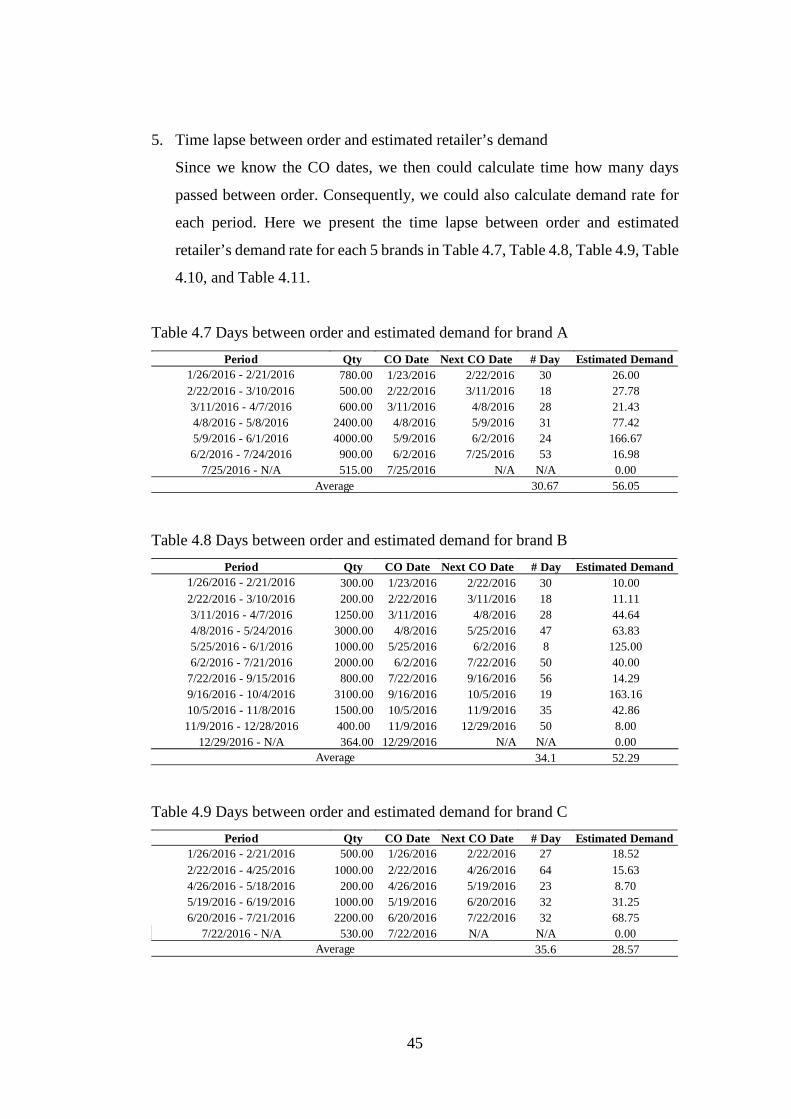
45
5. Time lapse between order and estimated retailer’s demand
Since we know the CO dates, we then could calculate time how many days
passed between order. Consequently, we could also calculate demand rate for
each period. Here we present the time lapse between order and estimated
retailer’s demand rate for each 5 brands in Table 4.7, Table 4.8, Table 4.9, Table
4.10, and Table 4.11.
Table 4.7 Days between order and estimated demand for brand A
Table 4.8 Days between order and estimated demand for brand B
Table 4.9 Days between order and estimated demand for brand C
Period Qty CO Date Next CO Date # Day Estimated Demand1/26/2016 - 2/21/2016 780.00 1/23/2016 2/22/2016 30 26.002/22/2016 - 3/10/2016 500.00 2/22/2016 3/11/2016 18 27.783/11/2016 - 4/7/2016 600.00 3/11/2016 4/8/2016 28 21.434/8/2016 - 5/8/2016 2400.00 4/8/2016 5/9/2016 31 77.425/9/2016 - 6/1/2016 4000.00 5/9/2016 6/2/2016 24 166.676/2/2016 - 7/24/2016 900.00 6/2/2016 7/25/2016 53 16.98
7/25/2016 - N/A 515.00 7/25/2016 N/A N/A 0.0030.67 56.05Average
Period Qty CO Date Next CO Date # Day Estimated Demand1/26/2016 - 2/21/2016 300.00 1/23/2016 2/22/2016 30 10.002/22/2016 - 3/10/2016 200.00 2/22/2016 3/11/2016 18 11.113/11/2016 - 4/7/2016 1250.00 3/11/2016 4/8/2016 28 44.644/8/2016 - 5/24/2016 3000.00 4/8/2016 5/25/2016 47 63.835/25/2016 - 6/1/2016 1000.00 5/25/2016 6/2/2016 8 125.006/2/2016 - 7/21/2016 2000.00 6/2/2016 7/22/2016 50 40.00
7/22/2016 - 9/15/2016 800.00 7/22/2016 9/16/2016 56 14.299/16/2016 - 10/4/2016 3100.00 9/16/2016 10/5/2016 19 163.1610/5/2016 - 11/8/2016 1500.00 10/5/2016 11/9/2016 35 42.8611/9/2016 - 12/28/2016 400.00 11/9/2016 12/29/2016 50 8.00
12/29/2016 - N/A 364.00 12/29/2016 N/A N/A 0.0034.1 52.29Average
Period Qty CO Date Next CO Date # Day Estimated Demand1/26/2016 - 2/21/2016 500.00 1/26/2016 2/22/2016 27 18.522/22/2016 - 4/25/2016 1000.00 2/22/2016 4/26/2016 64 15.634/26/2016 - 5/18/2016 200.00 4/26/2016 5/19/2016 23 8.705/19/2016 - 6/19/2016 1000.00 5/19/2016 6/20/2016 32 31.256/20/2016 - 7/21/2016 2200.00 6/20/2016 7/22/2016 32 68.75
7/22/2016 - N/A 530.00 7/22/2016 N/A N/A 0.0035.6 28.57Average
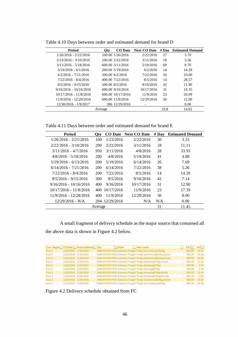
46
Table 4.10 Days between order and estimated demand for brand D
Table 4.11 Days between order and estimated demand for brand E
A small fragment of delivery schedule as the major source that contained all
the above data is shown in Figure 4.2 below.
Figure 4.2 Delivery schedule obtained from FC
Period Qty CO Date Next CO Date # Day Estimated Demand1/26/2016 - 2/22/2016 100.00 1/26/2016 2/22/2016 27 3.702/23/2016 - 3/10/2016 100.00 2/22/2016 3/11/2016 18 5.563/11/2016 - 5/18/2016 600.00 3/11/2016 5/19/2016 69 8.705/19/2016 - 6/1/2016 200.00 5/19/2016 6/2/2016 14 14.296/2/2016 - 7/21/2016 500.00 6/2/2016 7/22/2016 50 10.007/22/2016 - 8/4/2016 400.00 7/22/2016 8/5/2016 14 28.578/5/2016 - 9/15/2016 500.00 8/5/2016 9/16/2016 42 11.90
9/16/2016 - 10/16/2016 600.00 9/16/2016 10/17/2016 31 19.3510/17/2016 - 11/8/2016 600.00 10/17/2016 11/9/2016 23 26.0911/9/2016 - 12/29/2016 600.00 11/9/2016 12/29/2016 50 12.0012/30/2016 - 1/9/2017 306 12/29/2016 - 0.00
33.8 14.02Average
Period Qty CO Date Next CO Date # Day Estimated Demand1/26/2016 - 2/21/2016 100 1/23/2016 2/22/2016 30 3.332/22/2016 - 3/10/2016 200 2/22/2016 3/11/2016 18 11.113/11/2016 - 4/7/2016 950 3/11/2016 4/8/2016 28 33.934/8/2016 - 5/18/2016 200 4/8/2016 5/19/2016 41 4.88
5/19/2016 - 6/13/2016 200 5/19/2016 6/14/2016 26 7.696/14/2016 - 7/21/2016 200 6/14/2016 7/22/2016 38 5.267/22/2016 - 8/4/2016 200 7/22/2016 8/5/2016 14 14.298/5/2016 - 9/15/2016 300 8/5/2016 9/16/2016 42 7.14
9/16/2016 - 10/16/2016 400 9/16/2016 10/17/2016 31 12.9010/17/2016 - 11/8/2016 400 10/17/2016 11/9/2016 23 17.3911/9/2016 - 12/28/2016 400 11/9/2016 12/29/2016 50 8.00
12/29/2016 - N/A 204 12/29/2016 N/A N/A 0.0031 11.45Average
Cust. Region CO Date Actual Delivery City State Item name SO Qty mTonEast 2 1/26/2016 1/26/2016 KABUPATEN POSO Sulawesi Tengah Terigu Dua Pedang @25kg 500.00 12.50East 2 1/23/2016 1/26/2016 KABUPATEN POSO Sulawesi Tengah Terigu Gatotkaca@25kg plastik 780.00 19.50East 2 1/23/2016 1/26/2016 KABUPATEN POSO Sulawesi Tengah Terigu Gatotkaca@25kg plastik 780.00 19.50East 2 1/26/2016 1/26/2016 KABUPATEN POSO Sulawesi Tengah Terigu Kompas@25kg plastik 500.00 12.50East 2 1/26/2016 1/26/2016 KABUPATEN POSO Sulawesi Tengah Terigu Gerbang@25kg 100.00 2.50East 2 1/26/2016 1/26/2016 KABUPATEN POSO Sulawesi Tengah Terigu Gunung@25kg 100.00 2.50East 2 1/26/2016 1/26/2016 KABUPATEN POSO Sulawesi Tengah Terigu Kompas@25kg plastik 500.00 12.50East 2 1/23/2016 1/26/2016 KABUPATEN POSO Sulawesi Tengah Terigu Kompas@10kg/box (B) 300.00 3.00East 2 1/26/2016 1/26/2016 KABUPATEN POSO Sulawesi Tengah Terigu Gatotkaca@25kg plastik 780.00 19.50East 2 1/26/2016 1/26/2016 KABUPATEN POSO Sulawesi Tengah Terigu Dua Pedang @25kg 500.00 12.50

47
4.3 Data Collected on Procurement Department
Besides the delivery schedule, we also collected data via interview with
procurement officers about travel time and distance, alternative route, and penalty
cost in case delivery was late. We summarized the data collected as follows:
1. Regular or primary route of delivery from Makassar to Poso was using Trans-
Sulawesi road as depicted in Figure 4.3 below.
Figure 4.3 Primary route Makassar- Poso (source: maps.google.com)
According to the Figure 4.3 above, the travel time was 15 hours 20 minutes, in
reality truck drivers need to take breaks and stops a couple of times for the local
tax. Hence the actual travel time was 2 days. The distance also needs revision
because via interview, the actual regular distance was 689.4 Km.
2. Alternative route that typically used by truck drivers when the primary route
disrupted was via west coast, Makassar – Mamuju (West Sulawesi) – Poso. The
alternative route was depicted in Figure 4.4 and Figure 4.5 below.

48
Figure 4.4 Travel route from Makassar to Mamuju
Figure 4.5 Travel route from Mamuju to Poso
The actual accumulated travel time from Makassar – Mamuju – Poso was 4
days with 1040 Km accumulated distance.

49
3. Penalty costs due to lateness of delivery is usually charged by the customers to
the suppliers. In this case, there was no penalty costs charged by distributor to
FC when delivery was late. The only consequence due lateness was the risk of
having a bad reputation and the risk of loss of distributor’s willingness to
purchase (i.e. lowering the quantity of purchase order).
4. Freight Rate
Freight rate is a cost of hiring a truck with certain capacity on a specific
destination. A freight rate for a truck with 25 MT capacity destined to Poso was
Rp. 14.850.000. The rate per MT per Km was Rp 14.850.000 / (689.4*25) = Rp
861.62.
4.4 Data collected on Sales Department
We also collected data in respect of the selling price that FC charged for
each unit SKU that distributor order. The list of the selling price (ppn included) for
5 brands we selected was presented in Table 4.12 below.
Table 4.12 Brand’s selling price
4.5 Data Collected on BNPB
In order to cause a transportation disruption into the delivery process, we
collected data of natural disaster event from Badan Nasional Penanggulangan
Bencana (BNPB) via their website http://dibi.bnpb.go.id/data-bencana/crosstab.
Firstly, we determine the natural disaster affected area for South Sulawesi, since
traveling from Makassar to Poso is spending 80% of the distance through South
Sulawesi region. Secondly, we determine landslide, flood, and landslide-flood as
our focused natural disaster source, since this types are the major source of road
infrastructure failures in South Sulawesi. Thirdly, we determine 2001 to 2016 as
Brand Selling Price (per unit)A 133,100.00Rp B 80,000.00Rp C 152,000.00Rp D 155,000.00Rp E 162,800.00Rp

50
the years of observation. Lastly, we presented the frequency of natural disaster for
each year observed. The frequency of natural disaster is shown in Table 4.13 below.
Table 4.13 Frequency of natural disaster by year
4.6 Proposed Strategies and Impact Costs
Impact cost defined as the consequent cost incurred due to applying a
strategy. We proposed 4 strategies to mitigate negative impact of transportation
disruption, named: (1) Base Case; (2) Redundant Stock; (3) Flexible Route; and (4)
Redundant-Flexibility (ReFlex). For every strategy applied, the element of
transportation cost (TC) will always exist which expressed in Equation 4.1 below.
𝑇𝑇𝑇𝑇 = 𝑅𝑅𝑅𝑅𝑅𝑅𝑅𝑅 ∗ 𝑅𝑅𝑅𝑅𝑅𝑅𝑅𝑅𝑅𝑅𝑅𝑅𝑅𝑅 𝐷𝐷𝐷𝐷𝐷𝐷𝑅𝑅𝑅𝑅𝐷𝐷𝐷𝐷𝑅𝑅 ∗ 𝐷𝐷𝑅𝑅𝑅𝑅𝐷𝐷𝐷𝐷𝑅𝑅𝑅𝑅𝐷𝐷 𝑞𝑞𝑅𝑅𝐷𝐷/40 (4.1)
4.6.1 Base Case
FC would wait until the road is fixed, then started delivery, so it incurred an
extra holding cost (EHC) that depends on the holding costs (per unit per day),
disruption duration (DD), and delivery quantity being hold. Where the holding costs
equals to 30% of selling the brand’s selling price (BSP). Hence the impact costs of
this strategy was TC + EHC.
𝐸𝐸𝐸𝐸𝑇𝑇 = 𝐵𝐵𝐵𝐵𝐵𝐵∗𝑎𝑎𝑎𝑎𝑎𝑎𝑎𝑎𝑎𝑎𝑎𝑎 𝑣𝑣𝑎𝑎𝑎𝑎𝑎𝑎𝑣𝑣𝑣𝑣𝑝𝑝𝑣𝑣𝑝𝑝𝑝𝑝𝑝𝑝𝑝𝑝
∗ 𝐷𝐷𝐷𝐷 ∗ 𝐷𝐷𝑅𝑅𝑅𝑅𝐷𝐷𝐷𝐷𝑅𝑅𝑅𝑅𝐷𝐷 𝑞𝑞𝑅𝑅𝐷𝐷 (4.2)
where:
2001 2 2009 212002 3 2010 782003 5 2011 202004 12 2012 222005 5 2013 302006 25 2014 212007 32 2015 282008 34 2016 40
Year Frequency Year Frequency

51
𝐸𝐸𝐸𝐸𝑇𝑇 = extra holding costs (Rp)
𝐵𝐵𝐵𝐵𝐵𝐵 = selling price of the brand from FC to distributor (Rp)
𝐷𝐷𝐷𝐷 = the duration of disruption (day)
𝐵𝐵𝑅𝑅𝑅𝑅𝐷𝐷𝑃𝑃𝑃𝑃 = 365 days in a year
𝐴𝐴𝐷𝐷𝐷𝐷𝑅𝑅𝑅𝑅𝑅𝑅 𝐷𝐷𝑅𝑅𝑅𝑅𝑅𝑅𝑅𝑅𝐷𝐷 = set to be 30% or 0.3
4.6.2 Redundant Stock
Similar with base case, except in the very beginning of delivery period, FC
placed an extra inventory we called redundant stock in distributor’s warehouse.
Since redundant stock are kept in distributor’s warehouse, it is impractical if it
exclusively reserved in the case of disruption. In contrary, it can also use to satisfy
daily demand or to protect against lateness that caused by other factor than
disruption. Also to persuade distributor to kept the redundant stock in its warehouse,
the redundant holding cost (RHC) was paid 50% by FC. Therefore, the total
consequent costs of applying this strategy was the TC + EHC +RHC + redundant
transportation cost (RTC).
𝑅𝑅𝐸𝐸𝑇𝑇 = 𝑅𝑅 ∗ 𝐵𝐵𝐵𝐵𝐵𝐵 ∗ 𝑅𝑅𝐷𝐷𝐷𝐷𝑅𝑅𝑅𝑅𝑅𝑅 𝐷𝐷𝑅𝑅𝑅𝑅𝑅𝑅𝑅𝑅𝐷𝐷 ∗ 0.5 (4.3)
𝑅𝑅𝑇𝑇𝑇𝑇 = (𝑅𝑅/40) ∗ 𝑅𝑅𝑅𝑅𝑅𝑅𝑅𝑅 ∗ 𝑅𝑅𝑅𝑅𝑅𝑅𝑅𝑅𝑅𝑅𝑅𝑅𝑅𝑅 𝑃𝑃𝐷𝐷𝐷𝐷𝑅𝑅𝑅𝑅𝐷𝐷𝐷𝐷𝑅𝑅 (4.4)
where:
𝑅𝑅 = redundant stock quantity
4.6.3 Flexible Route
In this strategy, FC doesn’t have to wait until the road is fixed. FC persuade
the trucking company to use alternative route for the delivery process when the
transportation disruption occurred. When transportation disruption doesn’t occur
the truck used the regular route. As compensation, FC will pay additional cost
named extra distance costs (EDC) to the trucking company. In summary, the total
impact costs for this strategy was TC + EDC.
𝐸𝐸𝐷𝐷𝑇𝑇 = 𝑅𝑅𝑅𝑅𝑅𝑅𝑅𝑅 ∗ 𝐴𝐴𝑅𝑅𝑅𝑅𝑅𝑅𝑅𝑅𝐷𝐷𝑅𝑅𝑅𝑅𝐷𝐷𝐷𝐷𝑅𝑅 𝑃𝑃𝐷𝐷𝐷𝐷𝑅𝑅𝑅𝑅𝐷𝐷𝐷𝐷𝑅𝑅 ∗ (𝐷𝐷𝑅𝑅𝑅𝑅𝐷𝐷𝐷𝐷𝑅𝑅𝑅𝑅𝐷𝐷 𝑞𝑞𝑅𝑅𝐷𝐷/40 ) (4.5)
52
4.6.4 ReFlex
This strategy combined the redundant stock with flexible route. When
transportation disruption occurs truck will use the alternative route causing lateness
which is 4 days of trip. To cover this 4 days of lateness, in the very beginning of
period, FC placed a redundant stock equals to 4 days of demand (retailer’s). Hence,
the total impact costs of this strategy was TC + RHC + RTC + EDC.

53
CHAPTER 5
SIMULATION MODEL & CEA
This chapter shows how we conduct the simulation study and CEA by using
applying the specified methods from chapter 3 and collected data from chapter 4
5.1. Simulation Study
We conduct a simulation study according to the method we introduced in
Chapter 3.
5.1.1. Problem Formulation
We translate the Research Question (RQ) as the problem formulation for
this simulation study: “We don’t know the cost and effectiveness of each proposed
strategy against transportation disruption”
5.1.2. Setting Objectives
Based in the problem formulation, we defined the objective of this
simulation study as: “To find out the value of cost and effectiveness of each
proposed strategy”
5.1.3. Model Conceptualization
FC sells its products to the distributor where distributor re-sell the products
to retailers. Distributor act as a reseller who fills a known end retailer’s demand
from its inventory, which in turn is replenished by the FC. We assume that natural-
catastrophic events may occur at any point in time causing unavailability of road
infrastructure (main route) that connecting FC’s site with distributor site with a
frequency per year. Once a transportation disruption occurs, the ability of FC to
replenish distributor’s inventory stops temporarily (for the duration of the
disruption); however, retailer’s demand can continue to be met from inventory until
it is depleted. Depending on the duration of the disruption and on-hand inventory
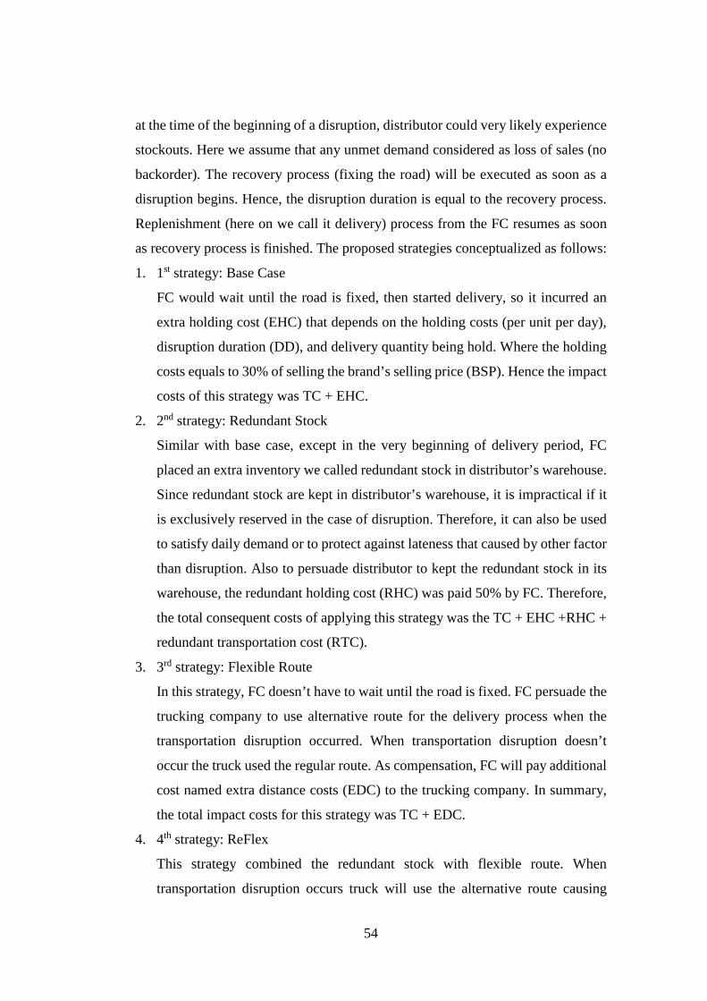
54
at the time of the beginning of a disruption, distributor could very likely experience
stockouts. Here we assume that any unmet demand considered as loss of sales (no
backorder). The recovery process (fixing the road) will be executed as soon as a
disruption begins. Hence, the disruption duration is equal to the recovery process.
Replenishment (here on we call it delivery) process from the FC resumes as soon
as recovery process is finished. The proposed strategies conceptualized as follows:
1. 1st strategy: Base Case
FC would wait until the road is fixed, then started delivery, so it incurred an
extra holding cost (EHC) that depends on the holding costs (per unit per day),
disruption duration (DD), and delivery quantity being hold. Where the holding
costs equals to 30% of selling the brand’s selling price (BSP). Hence the impact
costs of this strategy was TC + EHC.
2. 2nd strategy: Redundant Stock
Similar with base case, except in the very beginning of delivery period, FC
placed an extra inventory we called redundant stock in distributor’s warehouse.
Since redundant stock are kept in distributor’s warehouse, it is impractical if it
is exclusively reserved in the case of disruption. Therefore, it can also be used
to satisfy daily demand or to protect against lateness that caused by other factor
than disruption. Also to persuade distributor to kept the redundant stock in its
warehouse, the redundant holding cost (RHC) was paid 50% by FC. Therefore,
the total consequent costs of applying this strategy was the TC + EHC +RHC +
redundant transportation cost (RTC).
3. 3rd strategy: Flexible Route
In this strategy, FC doesn’t have to wait until the road is fixed. FC persuade the
trucking company to use alternative route for the delivery process when the
transportation disruption occurred. When transportation disruption doesn’t
occur the truck used the regular route. As compensation, FC will pay additional
cost named extra distance costs (EDC) to the trucking company. In summary,
the total impact costs for this strategy was TC + EDC.
4. 4th strategy: ReFlex
This strategy combined the redundant stock with flexible route. When
transportation disruption occurs truck will use the alternative route causing

55
lateness which is 4 days of trip. To cover this 4 days of lateness, in the very
beginning of period, FC placed a redundant stock equals to 4 days of demand
(retailer’s). Hence, the total impact costs of this strategy was TC + RHC + RTC
+ EDC.
We introduced 3 simulation logics to accommodate the coding process of the
proposed strategies. Each strategy consists of these simulation logic:
1. Delivery logic
This logic explains the delivery process from FC to distributor. Date of delivery
and quantity of each delivery are triggered by the delivery schedule. For the 1st
and 2nd strategy, the delivery is using regular route, either or not disruption
occur. For the 3rd and 4th strategy, when disruption not occur, use regular route.
But when disruption occur, use alternative route. When the delivered products
arrived at distributor’s site, the inventory instantly updated and the incurred cost
will be calculated.
2. Demand logic
This logic explains the process of how demands reducing the inventory level.
Demand assumed to be arrived every day with the rate for each period is
different from one another. Every time a demand arrived, inventory is used to
satisfy that demand. When demand cannot be satisfied, there will be a stockouts
under the assumption of no backorder. During the execution, this logic will
record the total number of unsatisfied demand.
3. Disruption logic
This logic generates occurrence of natural disaster that may or may not disturb
the delivery process. When a natural disaster happened at the same time with a
schedule delivery, then the delivery logic will be disrupted. For 1st and 2nd
strategy the delivery will not resume until the road is fixed. For 3rd and 4th the
delivery will use alternative route without waiting for the road to be fixed.
In summary, demand and disruption logic are the same on every strategy. But for
delivery logic, the construction will be different for each strategy. When simulating
every brand, the simulation input should have adjusted according to the correspond
brand.

56
5.1.4. Simulation Inputs Formulation
Using the method in Chapter 3, we could translate the data we have
collected to become simulation inputs. The formulation is presented in Table 5.1
below.
Table 5.1 Input for simulation study
Natural disaster occurrence was obtained by calculate the cumulative
distribution function (CDF) from data in Table 4.13 frequency of natural disaster
by year). The value of probability then used as the input in ARENA using
expression “DISC (upper limit, probability)”. The input value is presented in Table
5.2 below. As a remainder, there are 2 strategy using redundant stock which are 2nd
strategy (redundant stock) and 4th strategy (ReFlex). The quantity for each brand is
different according to the average days per period and average demand rate per
year. For example, quantity for brand A can be calculated using data from Table
4.7; for the 2nd strategy we’d like to protect the inventory for 1 period, thus equal
to 30.67 ∗ 56.05 = 1719.05 ≈ 1720 unit; for the 4th strategy we’d like to protect
the inventory for 4 days of transport time using alternative route, thus equal to 4 ∗
56.05 = 224.2 ≈ 225 unit. The same principal applied to other brand. Table 5.3
below shows the quantity of buffer stock for 5 brands in each strategy.
Collected Data Method to translate into simulation inputs Input valueDelivery date Use directly the data values See AppendixQuantity delivered Use directly the data values See AppendixRegular route travel time Guesstimate Constant: 2 daysAlternative route travel time Guesstimate Constant: 4 daysDemand date Use directly the data values See AppendixDemand quantity Use directly the data values See AppendixNatural disaster occurrence Empirical distribution function See Table 5.2Disruption duration Fit a probability distribution to the data values 0.14+LogN(3.19,8.64) daysRedundant stock quantity Use directly the data values See Table 5.3

57
Table 5.2 Simulation input for natural disaster occurrence
Table 5.3 Redundant stock quantity for 2nd and 4th strategy
5.1.5. Computerized Model in ARENA
We translated the conceptual model into computerized model using
simulation software package ARENA ®. We build the computerized model using
brand E since this brand has the least volume of delivery and the existence of
delivery for every month, thus the chance of having disruption is highly probable.
We start building the computerized model by translate the 3 logic we explained
before into the ARENA ®. We started from the 1st strategy way up to 4th strategy.
The computerized model of base case, redundant stock, flexible route, and ReFlex
are depicted consecutively in Figure 5.1, Figure 5.2, Figure 5.3, and Figure 5.4
below. We then conducted a pilot run of brand E for every strategy in a single
Lower limit Upper limit Probability0 5 0.255 10 0.25
10 15 0.3115 20 0.3820 25 0.6325 30 0.7530 35 0.8835 40 0.9440 45 0.9445 50 0.9450 55 0.9455 60 0.9460 65 0.9465 70 0.9470 75 0.9475 80 1.00
For 2nd strategy For 4th strategyA 1720 225B 1784 210C 1018 115D 474 57E 355 46
Redundant stock valueBrand

58
replication. The time unit for the simulation is in days with replication length for
368 days. To match the historic nature of the system under study, we start the
simulation from January 1st 2016.

59
Figure 5.1 Computerized model for base case strategy

60
Figure 5.2 Computerized model for redundant stock strategy

61
Figure 5.3 Computerized model for flexible route strategy

62
Figure 5.4 Computerized model for ReFlex strategy

63
5.1.6. Verification
We conduct a verification test by comparing the graphical output of
simulation with graphical output of hand calculations. We found that our
computerized model gave the same output as our hand calculations. The graphical
comparison between base case strategy was depicted in Figure 5.5; redundant
strategy in Figure 5.6; flexible route in Figure 5.7; and ReFlex in Figure 5.8.
Figure 5.5 Output comparison of hand calculations (top) with computerized model
(bottom) on base case

64
Figure 5.6 Output comparison of hand calculations (top) with computerized model
(bottom) on redundant stock strategy
Figure 5.7 Output comparison of hand calculations (top) with computerized model
(bottom) on flexible strategy
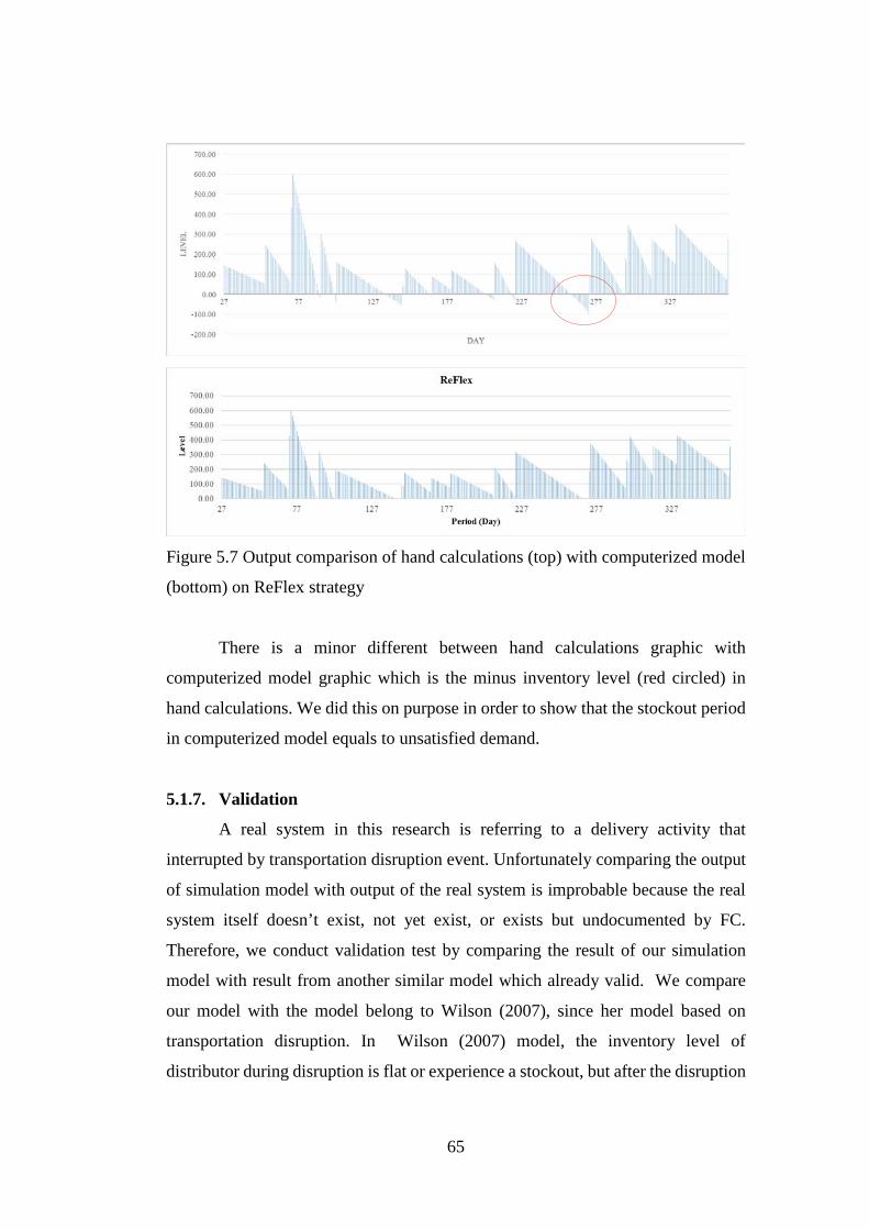
65
Figure 5.7 Output comparison of hand calculations (top) with computerized model
(bottom) on ReFlex strategy
There is a minor different between hand calculations graphic with
computerized model graphic which is the minus inventory level (red circled) in
hand calculations. We did this on purpose in order to show that the stockout period
in computerized model equals to unsatisfied demand.
5.1.7. Validation
A real system in this research is referring to a delivery activity that
interrupted by transportation disruption event. Unfortunately comparing the output
of simulation model with output of the real system is improbable because the real
system itself doesn’t exist, not yet exist, or exists but undocumented by FC.
Therefore, we conduct validation test by comparing the result of our simulation
model with result from another similar model which already valid. We compare
our model with the model belong to Wilson (2007), since her model based on
transportation disruption. In Wilson (2007) model, the inventory level of
distributor during disruption is flat or experience a stockout, but after the disruption
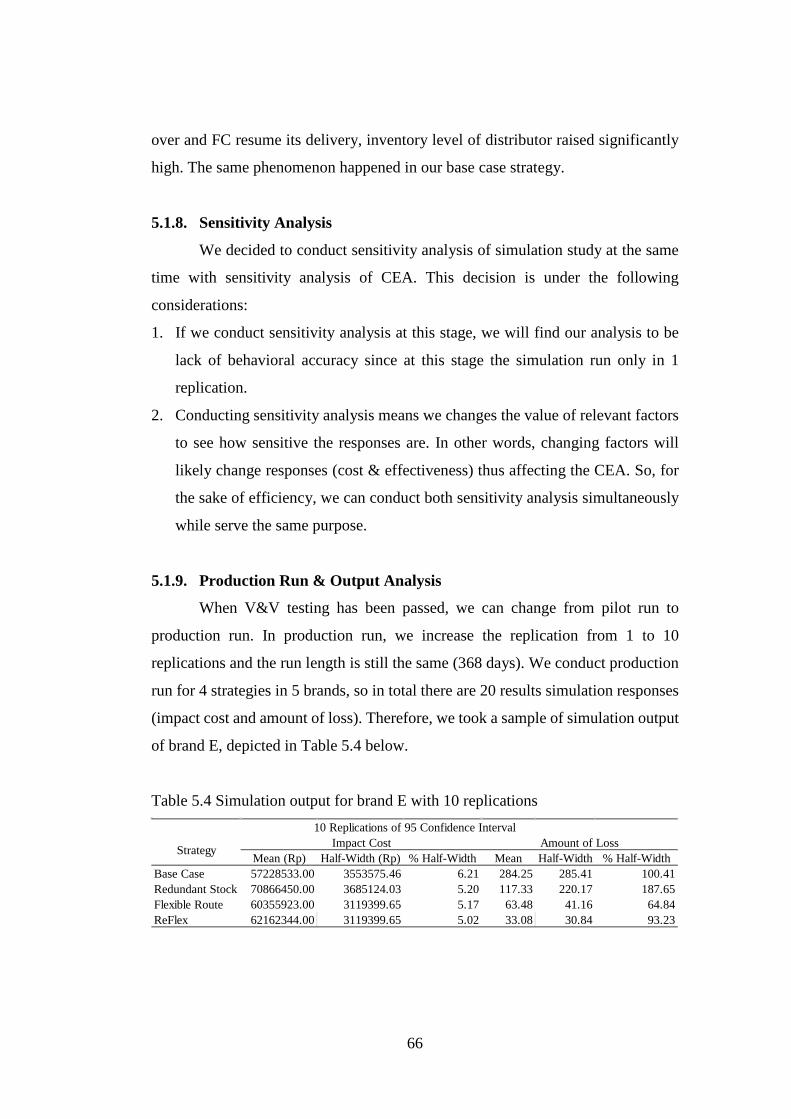
66
over and FC resume its delivery, inventory level of distributor raised significantly
high. The same phenomenon happened in our base case strategy.
5.1.8. Sensitivity Analysis
We decided to conduct sensitivity analysis of simulation study at the same
time with sensitivity analysis of CEA. This decision is under the following
considerations:
1. If we conduct sensitivity analysis at this stage, we will find our analysis to be
lack of behavioral accuracy since at this stage the simulation run only in 1
replication.
2. Conducting sensitivity analysis means we changes the value of relevant factors
to see how sensitive the responses are. In other words, changing factors will
likely change responses (cost & effectiveness) thus affecting the CEA. So, for
the sake of efficiency, we can conduct both sensitivity analysis simultaneously
while serve the same purpose.
5.1.9. Production Run & Output Analysis
When V&V testing has been passed, we can change from pilot run to
production run. In production run, we increase the replication from 1 to 10
replications and the run length is still the same (368 days). We conduct production
run for 4 strategies in 5 brands, so in total there are 20 results simulation responses
(impact cost and amount of loss). Therefore, we took a sample of simulation output
of brand E, depicted in Table 5.4 below.
Table 5.4 Simulation output for brand E with 10 replications
Mean (Rp) Half-Width (Rp) % Half-Width Mean Half-Width % Half-WidthBase Case 57228533.00 3553575.46 6.21 284.25 285.41 100.41Redundant Stock 70866450.00 3685124.03 5.20 117.33 220.17 187.65Flexible Route 60355923.00 3119399.65 5.17 63.48 41.16 64.84ReFlex 62162344.00 3119399.65 5.02 33.08 30.84 93.23
Impact Cost Amount of Loss10 Replications of 95 Confidence Interval
Strategy

67
From Figure 5.8 above, the half-width represents the simulation behavioral
accuracy under 95% confidence interval. For example, for base case strategy, with
95% C.I, the Mean for impact cost was Rp 70,866,450.00 with half-width Rp
3,685,124.03. It means that with 95% C.I we believe that the True Mean will fall
between the interval of Rp 70,866,450.00 ± Rp 3,685,124.03 or [Rp 74,551,574.03,
Rp 67,181,352.97]. While the amount of loss was 117.33 ± 220.17 or [337.5, -
102.84]. This interval for impact cost is quite wide, while the amount of loss shows
much wider interval which look unrealistic. The similar results were also found in
the other brand. It means that the bigger the half-width means the smaller the
accuracy of our simulation study. Therefore, we want to make this half-width value
smaller to get greater/better accuracy. One method that would approximately solve
this problem is by using Equation 3.1 to find 𝑛𝑛 number of replications larger than
10.
5.1.10. Replications
To find the number replications that give better accuracy, first we must set
target of how small the half-width we want. This target is subjectively set by analyst
and therefore, the new half-width value will just be an approximation value around
the target. In this research, we wanted to press the half-width value into 20 times
smaller. By Equation 3.1 it means that 𝑛𝑛 ≅ 10 (20)2 ,which 𝑛𝑛 equals to 4000
replications. Then we run the simulation again by changing 10 replications to 4000
replications.
5.1.11. Document Cost and Effectiveness
The results of simulation run for brand A, B, C, D, and E with 4000
replications compared with 10 replications was presented consecutively in Table
5.5, Table 5.6, Table 5.7, Table 5.8, and Table 5.9.

68
Table 5.5 Comparison of simulation output based on the number of replications for
brand A
Table 5.6 Comparison of simulation output based on the number of replications for
brand B
Mean (Rp) Half-Width (Rp) % Half-Width Mean Half-Width % Half-WidthBase Case 147289350.00 8656739.92 5.88 1663.76 1421.19 85.42Redundant Stock 207171186.00 8656739.92 4.18 711.90 1113.40 156.40Flexible Route 159790585.00 14301637.46 8.95 388.10 138.80 35.76ReFlex 167623964.00 14301637.46 8.53 180.56 121.58 67.33
Mean (Rp) Half-Width (Rp) % Half-Width Mean Half-Width % Half-WidthBase Case 143393372.00 179539.94 0.13 947.27 25.04 2.64Redundant Stock 203275208.00 179539.94 0.09 114.89 16.29 14.18Flexible Route 150869721.00 306782.72 0.20 716.52 10.69 1.49ReFlex 158703100.00 306782.72 0.19 497.87 10.36 2.08
Strategy Impact Cost Amount of Loss
10 Replications of 95 Confidence Interval
Strategy Impact Cost Amount of Loss
4000 Replications of 95 Confidence Interval
Mean (Rp) Half-Width (Rp) % Half-Width Mean Half-Width % Half-WidthBase Case 92087625.00 5721433.92 6.21 2045.77 1346.91 65.84Redundant Stock 124092600.00 5721433.92 4.61 876.74 1047.88 119.52Flexible Route 97897645.00 6308088.86 6.44 782.29 339.25 43.37ReFlex 101665046.00 6308088.86 6.20 572.29 339.25 59.28
Mean (Rp) Half-Width (Rp) % Half-Width Mean Half-Width % Half-WidthBase Case 88425475.00 156824.59 0.18 2571.22 51.94 2.02Redundant Stock 120430450.00 156824.59 0.13 1228.32 39.54 3.22Flexible Route 92704651.00 160794.17 0.17 2478.70 50.23 2.03ReFlex 96472053.00 160794.17 0.17 2291.99 49.17 2.15
10 Replications of 95 Confidence Interval
Strategy Impact Cost Amount of Loss
4000 Replications of 95 Confidence Interval
Strategy Impact Cost Amount of Loss

69
Table 5.7 Comparison of simulation output based on the number of replications for
brand C
Table 5.8 Comparison of simulation output based on the number of replications for
brand D
Mean (Rp) Half-Width (Rp) % Half-Width Mean Half-Width % Half-WidthBase Case 80059701.00 2739330.96 3.42 701.95 333.09 47.45Redundant Stock 118387422.00 2739330.96 2.31 82.16 137.10 166.87Flexible Route 85663678.00 4990628.49 5.83 548.59 230.43 42.00ReFlex 89993430.00 4990628.49 5.55 433.59 230.43 53.14
Mean (Rp) Half-Width (Rp) % Half-Width Mean Half-Width % Half-WidthBase Case 80380674.00 121683.01 0.15 1489.82 30.04 2.02Redundant Stock 118708395.00 121683.01 0.10 696.35 24.86 3.57Flexible Route 84475836.00 200454.25 0.24 1442.23 29.32 2.03ReFlex 88805589.00 200454.25 0.23 1329.63 29.21 2.20
10 Replications of 95 Confidence Interval
Strategy Impact Cost Amount of Loss
4000 Replications of 95 Confidence Interval
Strategy Impact Cost Amount of Loss
Mean (Rp) Half-Width (Rp) % Half-Width Mean Half-Width % Half-WidthBase Case 67362589.00 2991451.09 4.44 273.37 212.37 77.69Redundant Stock 85421999.00 2991451.09 3.50 59.56 77.11 129.46Flexible Route 72808077.00 3832785.05 5.26 63.68 33.65 52.84ReFlex 74979778.00 3832785.05 5.11 23.18 21.46 92.56
Mean (Rp) Half-Width (Rp) % Half-Width Mean Half-Width % Half-WidthBase Case 66868842.00 96444.19 0.14 312.63 7.64 2.44Redundant Stock 84928252.00 96444.19 0.11 40.61 5.08 12.51Flexible Route 70292619.00 114412.20 0.16 258.85 4.69 1.81ReFlex 72464320.00 114412.20 0.16 203.29 4.63 2.28
10 Replications of 95 Confidence Interval
Strategy Impact Cost Amount of Loss
4000 Replications of 95 Confidence Interval
Strategy Impact Cost Amount of Loss

70
Table 5.9 Comparison of simulation output based on the number of replications for
brand E
From these Table above, changing replications from 10 to 4000 replications, gave
significant improvement on the half-width value which for the impact cost the
percentage of half-width value was less than 1 % and for the amount of loss the
percentage of half-width value was less than 5%.
5.2. Cost-Effectiveness Analysis
Since running the simulation with 4000 replications gave better behavioral
accuracy of the simulation responses, in CEA we will use these values. For a detail
example of conducting CEA, will use simulation output from Table 5.9 of brand E
as input.
5.2.1. Obtain cost and effectiveness from simulation study We extract information from Table 5.9 so that we can focus on the cost and
effectiveness of each strategy for brand E.
Table 5.10 Impact cost (cost) and loss of sales (effectiveness) for brand E
Mean (Rp) Half-Width (Rp) % Half-Width Mean Half-Width % Half-WidthBase Case 57228533.00 3553575.46 6.21 284.25 285.41 100.41Redundant Stock 70866450.00 3685124.03 5.20 117.33 220.17 187.65Flexible Route 60355923.00 3119399.65 5.17 63.48 41.16 64.84ReFlex 62162344.00 3119399.65 5.02 33.08 30.84 93.23
Mean (Rp) Half-Width (Rp) % Half-Width Mean Half-Width % Half-WidthBase Case 55886922.06 76530.06 0.14 480.21 9.79 2.04Redundant Stock 69670332.00 79850.45 0.11 215.20 7.66 3.56Flexible Route 58545037.00 91154.85 0.16 452.21 8.94 1.98ReFlex 60351458.00 91154.85 0.15 407.79 8.87 2.18
Impact Cost Amount of Loss10 Replications of 95 Confidence Interval
4000 Replications of 95 Confidence IntervalImpact Cost Amount of Loss
Strategy
Strategy
Strategy Impact Cost Loss of Sales (%)Base Case 55,886,922.06Rp 12.79Redundant Stock 69,670,332.00Rp 5.24Flexible Route 58,545,037.00Rp 12.05ReFlex 60,351,458.00Rp 10.73

71
5.2.2. List Strategies in Ascending Order Then listed the strategies in ascending order either the for the impact cost or
for the % loss of sales. In this research, we list the strategies based on the % loss of
sales value, presented in Table 5.11 below.
Table 5.11 Strategies listed in ascending order
Carefully note that the lesser the loss of sales percentage, the bigger effectiveness
we gained, thus a small loss of sales percentage equals to big effectiveness. The
ascending order means that we set an order from the least effective to the greatest
effective.
5.2.3. Identify Weakly and/or Strongly Dominated Strategy From Table 5.11 above, we need to identify the weakly and/or strongly
dominated strategy. One easy way to identify is to hold on to a logic that with the
increasing cost comes increasing effectiveness. Firstly, move from base case to
flexible route, impact cost increase and the effectiveness also increase (lesser loss
of sales percentage); move from flexible route to ReFlex the cost also increases so
does the effectiveness; lastly move from ReFlex to redundant stock the cost also
increases and so does the effectiveness. Since the movement from one strategy to
another in an increasing order, this proves that there is no weakly or dominated
strategy.
5.2.4. Calculate ICER
Now we could calculate effectiveness ratios for each strategy using
Equation 2.1. The base case becomes the status-quo strategy; hence we didn’t
calculate its effectiveness ratio. Using Equation 2.1 the effectiveness for each
strategy is presented in Table 5.12 below.
Strategy Impact Cost Loss of Sales (%)Base Case 55,886,922.06Rp 12.79Flexible Route 58,545,037.00Rp 12.05ReFlex 60,351,458.00Rp 10.73Redundant Stock 69,670,332.00Rp 5.24

72
Table 5.12 Cost-effectiveness ratio for each strategy
5.2.5. Identify Extended Dominated Strategy From Table 5.12 above, the cost-effectiveness was presented as a negative
value which is unusual, but it is not wrong (we can safely ignore the negative sign).
The meaning of cost-effectiveness ratio is as follows: when we switch base case
with flexible route, then for every 1% decrement of loss of sales costs Rp
3,592,047.21; switching flexible route with ReFlex, then for every 1% decrement
of loss of sales costs Rp 1,368,500.76; switching ReFlex with redundant stock, then
for every 1% decrement of loss of sales costs Rp 1,697,426.96. As explained in
Chapter 2.5.1, an identification of extended dominated strategy will lead us towards
flexible route. The same logic in previous section could also applied to identify
extended dominated strategy, but this time we use the cost-effectiveness ratio. The
movement from one cost-effectiveness ratio to another should be in an increasing
manner (hence named incremental). Switching base case with flexible route doesn’t
show any problem, but when switching flexible route with ReFlex the movement is
not incremental. It means that switching base case with flexible route is not as cost-
effective as switching base case directly to ReFlex. Furthermore, switching base
case with ReFlex gives more effectiveness with lower cost that switching base case
with flexible route which gives lower effectiveness with more cost. Thus, we can
eliminate flexible route from Table 5.12 and recalculate the cost-effectiveness ratio,
as depicted in Table 5.13 below.
Table 5.13 Cost-effectiveness ratio after eliminate flexible route
Strategy Impact Cost Loss of Sales (%) ICERBase Case 55,886,922.06Rp 12.79Flexible Route 58,545,037.00Rp 12.05 (3,592,047.21)Rp ReFlex 60,351,458.00Rp 10.73 (1,368,500.76)Rp Redundant Stock 69,670,332.00Rp 5.24 (1,697,426.96)Rp
Strategy Impact Cost Loss of Sales (%) ICERBase Case 55,886,922.06Rp 12.79ReFlex 60,351,458.00Rp 10.73 (2,167,250.46)Rp Redundant Stock 69,670,332.00Rp 5.24 (1,697,426.96)Rp

73
When we take a look at cost-effectiveness ratio of ReFlex in Table 5.13, we
can clearly recognize that switching base case with ReFlex indeed gives greater
effectiveness with small cost increment. Once again we identify if any strategy is
extended dominated. By using the same principal when we screened out flexible
route, it is clear that ReFlex should be eliminated since this strategy extended
dominated by redundant stock. After eliminate ReFlex, then we can recalculate a
new cost-effectiveness ratio, which depicted in Table 5.14 below.
Table. 5.14 Cost-effectiveness ratio after eliminated ReFlex
Since there the cost-effectiveness ratio is on the right incremental order.
We can move to the next step by making an initial recommendation.
5.2.6. Introduce Initial Recommendation A kind reminder, that cost-effectiveness ratio is not a rank and only one
strategy can be applied/adopted. Therefore, instead of an instruction, an initial
recommendation was given to the decision maker so that they can decide which
strategy they should applied or perhaps choose to do nothing (base case). Decision
will be made based on the willingness-to-pay (WTP) which reflects the financial
capacity that the decision maker has. WTP will use cost-effectiveness ratio as its
measurement. WTP for each strategy is presented in Table 5.15 below.
Table 5.15 Initial recommended strategy for brand E
We can interpret this initial recommendation in Table 5.15 as the following:
1. If decision maker is only willing to pay less than Rp. 1,825,617.21 for every
1% decrement of loss of sales than it is suggested to applied base case strategy.
Strategy Impact Cost Loss of Sales (%) ICERBase Case 55,886,922.06Rp 12.79Redundant Stock 69,670,332.00Rp 5.24 (1,825,617.21)Rp
Recommended StrategyWTP ˂ 1,825,617.21Rp Base Case
1,825,617.21Rp ≥ WTP Redundant Stock
Willingness to Pay (WTP)

74
2. But if decision maker is willing to pay at least 1,825,617.21 and more for every
1% decrement of loss of sales than it is suggested to applied redundant stock as
mitigation strategy.
By using the same method for conducting CEA, we present the initial
recommendation for brand A, B, C, and D consecutively in Table 5.16, Table 5.17,
Table 5.18, and Table 5.19.
Table 5.16 Initial recommended strategy for brand A
Table 5.17 Initial recommended strategy for brand B
Table 5.18 Initial recommended strategy for brand C
Table 5.19 Initial recommended strategy for brand D
Recommended StrategyWTP ˂ 3,141,323.11Rp Base Case
3,141,323.11Rp to 3,305,222.21Rp Flexible Route3,305,223.21Rp to 11,115,237.90Rp ReFlex
11,115,238.90Rp ≥ WTP Redundant Stock
Willingness to Pay (WTP)
Recommended StrategyWTP ˂ 3,223,058.91Rp Base Case
3,223,058.91Rp ≥ WTP Redundant Stock
Willingness to Pay (WTP)
Recommended StrategyWTP ˂ 2,178,277.66Rp Base Case
2,178,277.66Rp to 2,319,278.07Rp Flexible Route2,319,279.07Rp ≥ WTP Redundant Stock
Willingness to Pay (WTP)
Recommended StrategyWTP ˂ 2,256,241.13Rp Base Case
2,256,241.13Rp to 3,424,156.14Rp ReFlex3,424,156.14Rp ≥ WTP Redundant Stock
Willingness to Pay (WTP)
75
CHAPTER 6
ANALYSIS & FINDINGS
This chapter shows how we conduct sensitivity analysis by changing
specific factors for each brand and analyze changes in responses and
recommendations. Then we presented the findings.
6.1. Sensitivity Analysis
We conduct a sensitivity analysis by changing relevant factor of each
strategy. Sensitivity analysis will serve 2 purposes as the following:
1. Simulation study: Finding out how sensitive a response change when the factors
are changing
2. CEA: Finding out how sensitive the initial recommendation when the responses
are changing.
These purposes are interrelated to each other because factors are affecting
responses and responses are affecting the recommendation. We changed certain
factors that relevant/important for certain strategy, except for base case. This
important factors will change the responses of the corresponds strategy. The
responses are impact cost and loss of sales percentage. For redundant stock strategy
the important factor is the stock that kept as a buffer in distributor’s warehouse. We
will reduce the initial stock value by 50% as the new stock value. For flexible route
strategy, the important factor is the alternative route travel time. Here we assumed
that truck company is able to reduce the transport time via alternative route in such
a way (i.e. cutting breaks) that the transport time is 3 days from formerly 4 days.
For ReFlex strategy, the important factors are the stock and the alternative route
travel time. The alternative route travel time will be reduced to 3 days and the stock
will be increased by 400%. The reason we increased stock in ReFlex but decrease
50% in redundant stock is to serve the second purpose we mentioned earlier. Since
ReFlex has 2 important factors then, the value combination between stock and
travel time would use 2k Factorial Designs, with 𝑘𝑘 = 2. We divided the work of

76
sensitivity analysis based on brand. We also made notations of BC (base case), RS
(redundant stock), FR (flexible route), and RF (ReFlex). Every notation will be
accompanied by a number, where 0 (zero) refers to the initial value in the
correspond strategy, any number other than 0 is the new developed strategy with
different assigned value for the purpose of this analysis. For example, RS-0 means
that this is redundant strategy with initial assigned value, where RS-1 is the
development strategy of RS-0 with different adjusted value. Every new strategy
(i.e. RS-1) will be simulated with the same run parameters of the original strategy.
6.2. Findings on Brand A
We developed new strategies by changing the value of the factors for each
strategy, run the new strategies, and document responses in the following Table 6.1.
Table 6.1 Factors variation on brand A
6.2.1. Factors and Responses Relationship
From Table 6.1 above, we then analyze each strategy to draw conclusion
about the relationship between factors and responses:
1. Redundant stock: Decreasing stock from 1720 to 860 unit was decreasing cost by Rp 11,932,521 but increasing loss by 0.93 %.
Notation Stock Total Impact Cost % LossRS-0 1720 203,275,208.00Rp 1.01RS-1 860 191,342,687.00Rp 1.94
860 11,932,521.00Rp -0.93

77
2. Flexible Route: Speeding up trans time from 4 to 3 days doesn't have any effect
on cost but decrease loss by 0.23 %.
3. ReFlex: Speeding up trans time from 4 days to 3 days doesn't have any effect
on cost but decrease % loss by 0.137; Adding up stock from 210 to 840 unit
increase the cost by Rp 23,500,139 but decrease % loss by 4.26.
6.2.2. Final Recommendation
We used responses from Table 6.1 of all notations to perform sensitivity
analysis on CEA (SA-CEA) as presented in Table 6.2 and Table 6.3 while a
generated final recommendation presented in Table 6.4.
Table 6.2 Ascending order of SA-CEA for brand A
Notation Trans.Time Total Impact Cost % LossFR-0 4 150,869,721.00Rp 7.39FR-1 3 150,869,721.00Rp 7.16
1 0.00 0.23
Notation Trans.time Stock Cost % LossRF-0 4 225 158,703,100.00Rp 5.02RF-1 3 225 158,703,100.00Rp 4.81RF-3 4 900 182,203,239.00Rp 0.68RF-2 3 900 182,203,239.00Rp 0.62
Notation Total Impact Cost % LossBC 143,393,372.00Rp 9.77FR-0 150,869,721.00Rp 7.39FR-1 150,869,721.00Rp 7.16RF-0 158,703,100.00Rp 5.02RF-1 158,703,100.00Rp 4.81RS-1 191,342,687.00Rp 1.94RS-0 203,275,208.00Rp 1.01RF-3 182,203,239.00Rp 0.68RF-2 182,203,239.00Rp 0.62

78
Table 6.3 Elimination of dominated strategies of SA-CEA for brand A
Table 6.4 Final recommendation for brand A
By changing factors in simulation study and generate new strategies, it would or
would not generate a new recommendation. A comparison of the initial
recommendation in Table 5.16 and the final recommendation in Table 6.4 gave us
several findings as follows:
1. We changed the factors hence generated 5 new strategies, but there it didn’t
change the number of recommended strategy from initial to final.
2. Speeding up the alternative route travel time not only replacing RF-0 with RF-
1 but also replacing FR-0 with FR-1;
3. Speeding up the alternative route travel time from 4 to 3 days and adds up stock
by 400% make RF-2 less costly and more effective, hence replacing RS-0;
4. The WTP interval for all recommended strategy is decrease.
6.3. Findings on Brand B
We developed new strategies by changing the value of the factors for each
strategy, run the new strategies, and document responses in the following Table 6.5.
Notation Total Impact Cost % Loss ICERBC 143,393,372.00Rp 9.77 Status-quoFR-0 150,869,721.00Rp 7.39 Weakly dominatedFR-1 150,869,721.00Rp 7.16 (2,868,009.48)Rp RF-0 158,703,100.00Rp 5.02 Weakly dominatedRF-1 158,703,100.00Rp 4.81 (3,325,809.03)Rp RS-1 191,342,687.00Rp 1.94 Strongly dominatedRS-0 203,275,208.00Rp 1.01 Strongly dominatedRF-3 182,203,239.00Rp 0.68 Weakly dominatedRF-2 182,203,239.00Rp 0.62 (5,609,662.03)Rp
Recommended StrategyWTP ˂ 2,868,009.48Rp BC
2,868,009.48Rp to 3,325,808.03Rp FR-13,325,809.03Rp to 5,609,661.03Rp RF-15,609,662.03Rp ≥ WTP RF-2
Willingness to Pay (WTP)

79
Table 6.5 Factors variation on brand B
6.3.1. Factors and Responses Relationship
From Table 6.5 above, we then analyze each strategy to draw conclusion
about the relationship between factors and responses:
4. Redundant stock: Decreasing stock from 1784 to 892 unit decreasing cost by
Rp 16,002,488 but increase % loss by 4.83.
5. Flexible Route: Speeding up trans time from 4 to 3 days doesn't have any effect
of cost but decrease loss by 0.03 %
6. ReFlex: Speeding up trans time from 4 days to 3 days doesn't have any effect
on cost but decrease % loss by 0.026; Adding up stock from 210 to 840 unit
increase the cost by Rp 11,302,205 but decrease % loss by 3.83.
Trans. Time Stock Total Impact Cost Loss of sales Total QtyBC N/A N/A 88,425,475.00Rp 2571.22 14856 17.31FR-1 3 N/A 92,704,651.00Rp 2474.29 14856 16.66FR-0 4 N/A 92,704,651.00Rp 2478.70 14856 16.68RS-0 N/A 1784 120,430,450.00Rp 1228.32 16640 7.38RS-1 N/A 892 104,427,962.00Rp 1922.68 15748 12.21RF-1 3 210 96,472,053.00Rp 2287.85 15066 15.19RF-2 3 840 107,774,258.00Rp 1782.90 15696 11.36RF-0 4 210 96,472,053.00Rp 2291.99 15066 15.21RF-3 4 840 107,774,258.00Rp 1786.82 15696 11.38
NotationFactors Responses
% Loss
Notation Stock Total Impact Cost % LossRS-0 1784 120,430,450.00Rp 7.38RS-1 892 104,427,962.00Rp 12.21
892 16,002,488.00Rp -4.83
Notation Trans.Time Total Impact Cost % LossFR-0 4 92,704,651.00Rp 16.68FR-1 3 92,704,651.00Rp 16.66
1 0.00 0.03
Notation Trans.time Stock Cost % LossRF-0 4 210 96,472,053.00Rp 15.21RF-1 3 210 96,472,053.00Rp 15.19RF-3 4 840 107,774,258.00Rp 11.38RF-2 3 840 107,774,258.00Rp 11.36

80
6.3.2. Final Recommendation
We used responses from Table 6.5 of all notations to perform sensitivity
analysis on CEA (SA-CEA) as presented in Table 6.6 and Table 6.7 while a
generated final recommendation presented in Table 6.8.
Table 6.6 Ascending order of SA-CEA for brand B
Table 6.7 Elimination of dominated strategies of SA-CEA for brand B
Table 6.8 Final recommendation for brand B
By changing factors in simulation study and generate new strategies, it would or
would not generate a new recommendation. A comparison of the initial
recommendation in Table 5.17 and the final recommendation in Table 6.8 gave us
several findings as follows:
Notation Total Impact Cost % LossBC 88,425,475.00Rp 17.31FR-0 92,704,651.00Rp 16.68FR-1 92,704,651.00Rp 16.66RF-0 96,472,053.00Rp 15.21RF-1 96,472,053.00Rp 15.19RS-1 104,427,962.00Rp 12.21RF-3 107,774,258.00Rp 11.38RF-2 107,774,258.00Rp 11.36RS-0 120,430,450.00Rp 7.38
Notation Total Impact Cost % Loss ICERBC 88,425,475.00Rp 17.31 -FR-0 92,704,651.00Rp 16.68 Weakly dominatedFR-1 92,704,651.00Rp 16.66 Extended dominatedRF-0 96,472,053.00Rp 15.21 Weakly dominatedRF-1 96,472,053.00Rp 15.19 Extended dominatedRS-1 104,427,962.00Rp 12.21 (3,138,618.04)Rp RF-3 107,774,258.00Rp 11.38 Weakly dominatedRF-2 107,774,258.00Rp 11.36 Extended dominatedRS-0 120,430,450.00Rp 7.38 (3,314,989.62)Rp
Recommended StrategyWTP ˂ 3,138,618.04Rp BC
3,138,618.04Rp to 3,314,988.62Rp RS-13,314,989.62Rp ≥ WTP RS-0
Willingness to Pay (WTP)
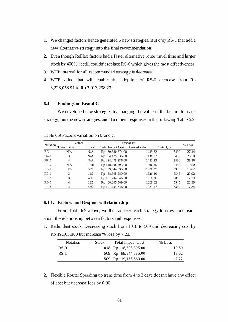
81
1. We changed factors hence generated 5 new strategies. But only RS-1 that add a
new alternative strategy into the final recommendation;
2. Even though ReFlex factors had a faster alternative route travel time and larger
stock by 400%, it still couldn’t replace RS-0 which gives the most effectiveness;
3. WTP interval for all recommended strategy is decrease.
4. WTP value that will enable the adoption of RS-0 decrease from Rp
3,223,058.91 to Rp 2,013,298.23;
6.4. Findings on Brand C
We developed new strategies by changing the value of the factors for each
strategy, run the new strategies, and document responses in the following Table 6.9.
Table 6.9 Factors variation on brand C
6.4.1. Factors and Responses Relationship
From Table 6.9 above, we then analyze each strategy to draw conclusion
about the relationship between factors and responses:
1. Redundant stock: Decreasing stock from 1018 to 509 unit decreasing cost by
Rp 19,163,860 but increase % loss by 7.22.
2. Flexible Route: Speeding up trans time from 4 to 3 days doesn't have any effect
of cost but decrease loss by 0.06
Trans. Time Stock Total Impact Cost Loss of sales Total QtyBC N/A N/A 80,380,674.00Rp 1489.82 5430 27.44FR-1 3 N/A 84,475,836.00Rp 1438.92 5430 26.50FR-0 4 N/A 84,475,836.00Rp 1442.23 5430 26.56RS-0 N/A 1018 118,708,395.00Rp 696.35 6448 10.80RS-1 N/A 509 99,544,535.00Rp 1070.27 5939 18.02RF-1 3 115 88,805,589.00Rp 1326.40 5545 23.92RF-2 3 460 101,794,846.00Rp 1018.26 5890 17.29RF-0 4 115 88,805,589.00Rp 1329.63 5545 23.98RF-3 4 460 101,794,846.00Rp 1021.17 5890 17.34
% LossNotationFactors Responses
Notation Stock Total Impact Cost % LossRS-0 1018 118,708,395.00Rp 10.80RS-1 509 99,544,535.00Rp 18.02
509 19,163,860.00Rp -7.22

82
3. ReFlex: Speeding up trans time from 4 days to 3 days doesn't have any effect
on cost but decrease % loss by 0.054; Adding up stock from 115 to 460 unit
increase the cost by Rp 12,989,257 but decrease % loss by 6.64.
6.4.2. Final Recommendation
We used responses from Table 6.9 of all notations to perform sensitivity
analysis on CEA (SA-CEA) as presented in Table 6.10 and Table 6.11 while a
generated final recommendation presented in Table 6.12.
Table 6.10 Ascending order of SA-CEA for brand C
Notation Trans.Time Total Impact Cost % LossFR-0 4 84,475,836.00Rp 26.56FR-1 3 84,475,836.00Rp 26.50
1 0.00 0.06
Notation Trans.time Stock Cost % LossRF-0 4 115 88,805,589.00Rp 23.98RF-1 3 115 88,805,589.00Rp 23.92RF-3 4 460 101,794,846.00Rp 17.34RF-2 3 460 101,794,846.00Rp 17.29
Notation Total Impact Cost % LossBC 80,380,674.00Rp 27.44FR-0 84,475,836.00Rp 26.56FR-1 84,475,836.00Rp 26.50RF-0 88,805,589.00Rp 23.98RF-1 88,805,589.00Rp 23.92RS-1 99,544,535.00Rp 18.02RF-3 101,794,846.00Rp 17.34RF-2 101,794,846.00Rp 17.29RS-0 118,708,395.00Rp 10.80

83
Table 6.11 Elimination of dominated strategies of SA-CEA for brand C
Table 6.12 Final recommendation for brand C
By changing factors in simulation study and generate new strategies, it would or
would not generate a new recommendation. A comparison of the initial
recommendation in Table 5.18 and the final recommendation in Table 6.12 gave us
several findings as follows:
1. Even though we changed factors and generated 5 additional strategies, the
number of recommended strategy didn’t change from the initial to final.
2. Changing the important factors only replaced FR-0 from initial
recommendation with RS-1 in the final recommendation;
3. Even though ReFlex factors had a faster alternative route travel time and larger
stock by 400%, it still couldn’t replace RS-0.
4. WTP value that will enable the application of RS-0 increased from Rp
2,319,279.07 to Rp 2,653,695.49
6.5. Findings on Brand D
We developed new strategies by changing the value of the factors for each
strategy, run the new strategies, and document responses in the following Table
6.13.
Notation Total Impact Cost % Loss ICERBC 80,380,674.00Rp 27.44 -FR-0 84,475,836.00Rp 26.56 Weakly dominatedFR-1 84,475,836.00Rp 26.50 Extended dominatedRF-0 88,805,589.00Rp 23.98 Weakly dominatedRF-1 88,805,589.00Rp 23.92 Extended dominatedRS-1 99,544,535.00Rp 18.02 (2,035,290.82)Rp RF-3 101,794,846.00Rp 17.34 Weakly dominatedRF-2 101,794,846.00Rp 17.29 Extended dominatedRS-0 118,708,395.00Rp 10.80 (2,653,695.49)Rp
Recommended StrategyWTP ˂ 2,035,290.82Rp BC
2,035,290.82Rp to 2,653,694.49Rp RS-12,653,695.49Rp ≥ WTP RS-0
Willingness to Pay (WTP)

84
Table 6.13 Factors variation on brand D
6.5.1. Factors and Responses Relationship
From Table 6.13 above, we then analyze each strategy to draw conclusion
about the relationship between factors and responses:
1. Redundant stock: Decreasing stock from 474 to 237 unit decreasing cost by Rp
9,029,705 but increase % loss by 1.81.
2. Flexible Route: Speeding up trans time from 4 to 3 days doesn't have any effect
of cost but decrease loss by 0.004.
ReFlex: Speeding up trans time from 4 days to 3 days doesn't have any effect on
cost but decrease % loss by 0.035; Adding up stock from 57 to 284 unit increase
the cost by Rp 6,515,104.00 but decrease % loss by 2.85.
Trans. Time Stock Total Impact Cost Loss of salesBC N/A N/A 66,868,842.00Rp 312.63 4506 6.94FR-1 3 N/A 70,292,619.00Rp 256.82 4506 5.70FR-0 4 N/A 70,292,619.00Rp 258.85 4506 5.74RS-0 N/A 474 84,928,252.00Rp 40.61 4980 0.82RS-1 N/A 237 75,898,547.00Rp 124.94 4743 2.63RF-1 3 57 72,464,320.00Rp 201.34 4563 4.41RF-2 3 228 78,979,424.00Rp 74.89 4734 1.58RF-0 4 57 72,464,320.00Rp 203.29 4563 4.46RF-3 4 228 78,979,424.00Rp 75.92 4734 1.60
NotationFactors Responses
Total Qty % Loss
Notation Stock Total Impact Cost % LossRS-0 474 84,928,252.00Rp 0.82RS-1 237 75,898,547.00Rp 2.63
237 9,029,705.00Rp -1.81
Notation Trans.Time Total Impact Cost % LossFR-0 4 70,292,619.00Rp 5.74FR-1 3 70,292,619.00Rp 5.70
1 0.00 0.04
Notation Trans.time Stock Cost % LossRF-0 4 57 72,464,320.00Rp 4.46RF-1 3 57 72,464,320.00Rp 4.41RF-3 4 228 78,979,424.00Rp 1.60RF-2 3 228 78,979,424.00Rp 1.58

85
6.5.2. Final Recommendation
We used responses from Table 6.13 of all notations to perform sensitivity
analysis on CEA (SA-CEA) as presented in Table 6.14 and Table 6.15 while a
generated final recommendation presented in Table 6.16.
Table 6.14 Ascending order of SA-CEA for brand D
Table 6.15 Elimination of dominated strategies of SA-CEA for brand D
Table 6.16 Final recommendation for brand D
By changing factors in simulation study and generate new strategies, it would or
would not generate a new recommendation. A comparison of the initial
recommendation in Table 5.19 and the final recommendation in Table 6.16 gave us
several findings as follows:
Notation Total Impact Cost % LossBC 66,868,842.00Rp 6.94FR-0 70,292,619.00Rp 5.74FR-1 70,292,619.00Rp 5.70RF-0 72,464,320.00Rp 4.46RF-1 72,464,320.00Rp 4.41RS-1 75,898,547.00Rp 2.63RF-3 78,979,424.00Rp 1.60RF-2 78,979,424.00Rp 1.58RS-0 84,928,252.00Rp 0.82
Notation Total Impact Cost % Loss ICERBC 66,868,842.00Rp 6.94 -FR-0 70,292,619.00Rp 5.74 Weakly dominatedFR-1 70,292,619.00Rp 5.70 Extended dominatedRF-0 72,464,320.00Rp 4.46 Weakly dominatedRF-1 72,464,320.00Rp 4.41 Extended dominatedRS-1 75,898,547.00Rp 2.63 (2,098,035.95)Rp RF-3 78,979,424.00Rp 1.60 Weakly dominatedRF-2 78,979,424.00Rp 1.58 (2,927,782.42)Rp RS-0 84,928,252.00Rp 0.82 (7,761,558.26)Rp
Recommended StrategyWTP ˂ 2,098,035.95Rp BC
2,098,035.95Rp to 2,927,781.42Rp RS-12,927,782.42Rp to 7,761,558.26Rp RF-27,761,558.26Rp ≥ WTP RS-0
Willingness to Pay (WTP)

86
1. There is new additional strategy into the final recommendation which is RS-1;
2. Changing the factors only replacing RF-0 from initial recommendation with
RF-1 in final recommendation;
3. Even though ReFlex factors had a faster alternative route travel time and larger
stock by 400%, it still couldn’t replace RS-0 that gives the greatest
effectiveness;
4. WTP value for RS-0 increased from Rp 3,424,156.14 to Rp 7,761,558.26.
6.6. Findings on Brand E
We developed new strategies by changing the value of the factors for each
strategy, run the new strategies, and document responses in the following Table
6.17.
Table 6.17 Factors variation on brand E
6.6.1. Factors and Responses Relationship
From Table 6.17 above, we then analyze each strategy to draw conclusion
about the relationship between factors and responses:
1. Redundant stock: Decreasing up stock from 355 to 178 unit decreasing cost by
Rp 6,950,794 but increase % loss by 3.45.
Trans. Time Stock Total Impact Cost Amount of Loss Total QtyBC N/A N/A 55,886,922.06Rp 312.63 3754 12.79FR-1 3 N/A 58,545,037.00Rp 451.09 3754 12.02FR-0 4 N/A 58,545,037.00Rp 452.21 3754 12.05RS-0 N/A 355 69,670,332.00Rp 215.20 4109 5.24RS-1 N/A 178 62,719,538.00Rp 341.68 3932 8.69RF-1 3 46 60,351,458.00Rp 406.72 3800 10.70RF-2 3 184 65,770,721.00Rp 290.74 3938 7.38RF-0 4 46 60,351,458.00Rp 407.79 3800 10.73RF-3 4 184 65,770,721.00Rp 291.61 3938 7.41
% LossNotation ResponsesFactors
Notation Stock Total Impact Cost % LossRS-0 355 69,670,332.00Rp 5.24RS-1 178 62,719,538.00Rp 8.69
177 6,950,794.00Rp -3.45
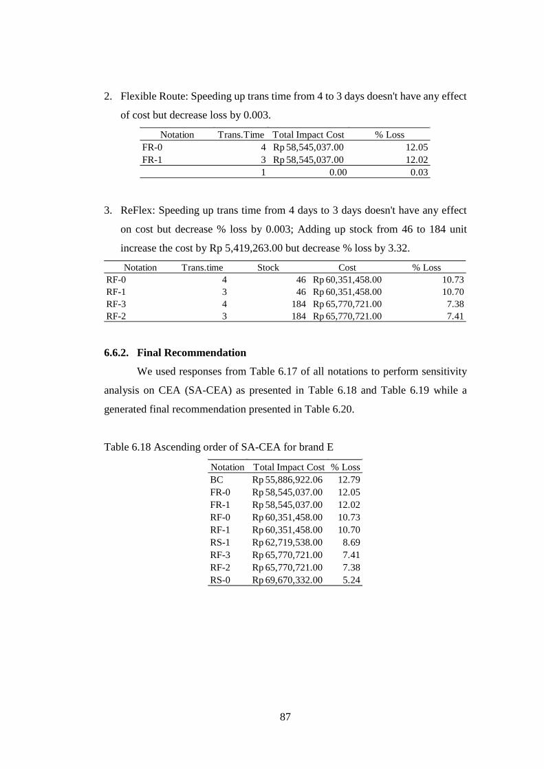
87
2. Flexible Route: Speeding up trans time from 4 to 3 days doesn't have any effect
of cost but decrease loss by 0.003.
3. ReFlex: Speeding up trans time from 4 days to 3 days doesn't have any effect
on cost but decrease % loss by 0.003; Adding up stock from 46 to 184 unit
increase the cost by Rp 5,419,263.00 but decrease % loss by 3.32.
6.6.2. Final Recommendation
We used responses from Table 6.17 of all notations to perform sensitivity
analysis on CEA (SA-CEA) as presented in Table 6.18 and Table 6.19 while a
generated final recommendation presented in Table 6.20.
Table 6.18 Ascending order of SA-CEA for brand E
Notation Trans.Time Total Impact Cost % LossFR-0 4 58,545,037.00Rp 12.05FR-1 3 58,545,037.00Rp 12.02
1 0.00 0.03
Notation Trans.time Stock Cost % LossRF-0 4 46 60,351,458.00Rp 10.73RF-1 3 46 60,351,458.00Rp 10.70RF-3 4 184 65,770,721.00Rp 7.38RF-2 3 184 65,770,721.00Rp 7.41
Notation Total Impact Cost % LossBC 55,886,922.06Rp 12.79FR-0 58,545,037.00Rp 12.05FR-1 58,545,037.00Rp 12.02RF-0 60,351,458.00Rp 10.73RF-1 60,351,458.00Rp 10.70RS-1 62,719,538.00Rp 8.69RF-3 65,770,721.00Rp 7.41RF-2 65,770,721.00Rp 7.38RS-0 69,670,332.00Rp 5.24

88
Table 6.19 Elimination of dominated strategies of SA-CEA for brand E
Table 6.20 Final recommendation for brand E
By changing factors in simulation study and generate new strategies, it would or
would not generate a new recommendation. A comparison of the initial
recommendation in Table 5.15 and the final recommendation in Table 6.20 gave us
several findings as follows:
1. There is new additional strategy into the final recommendation which is RS-1;
2. Even though ReFlex factors had a faster alternative route travel time and larger
stock by 400%, it still couldn’t replace RS-0 that gives the greatest
effectiveness;
3. WTP value for RS-0 increased from Rp 1,825,617.21 to Rp 2,013,298.23.
6.7. Analysis on Findings
An analysis on findings conducted across all brands a behavior peculiarity
has been founded. A comparison between the initial recommendation and final
recommendation for brand A, B, C, D, and E, respectively shown in Figure 6.1,
Figure 6.2, Figure 6.3, Figure 6.4, and Figure 6.5 as follows
Notation Total Impact Cost % Loss ICERBC 55,886,922.06Rp 12.79 -FR-0 58,545,037.00Rp 12.05 Weakly dominatedFR-1 58,545,037.00Rp 12.02 Extended dominatedRF-0 60,351,458.00Rp 10.73 Weakly dominatedRF-1 60,351,458.00Rp 10.70 Extended dominatedRS-1 62,719,538.00Rp 8.69 (1,666,380.06)Rp RF-3 65,770,721.00Rp 7.41 Weakly dominatedRF-2 65,770,721.00Rp 7.38 Extended dominatedRS-0 69,670,332.00Rp 5.24 (2,013,298.23)Rp
Recommended StrategyWTP ˂ 1,666,380.06Rp BC
1,666,380.06Rp to 2,013,297.23Rp RS-12,013,298.23Rp ≥ WTP RS-0
Willingness to Pay (WTP)

89
Figure 6.1 Comparison between initial recommendation (top) with final
recommendation (below) for brand A
Figure 6.2 Comparison between initial recommendation (top) with final
recommendation (below) for brand B
Figure 6.3 Comparison between initial recommendation (top) with final
recommendation (below) for brand C
Recommended StrategyWTP ˂ 3,141,323.11Rp Base Case
3,141,323.11Rp to 3,305,222.21Rp Flexible Route3,305,223.21Rp to 11,115,237.90Rp ReFlex
11,115,238.90Rp ≥ WTP Redundant Stock
Willingness to Pay (WTP)
Recommended StrategyWTP ˂ 2,868,009.48Rp BC
2,868,009.48Rp to 3,325,808.03Rp FR-13,325,809.03Rp to 5,609,661.03Rp RF-15,609,662.03Rp ≥ WTP RF-2
Willingness to Pay (WTP)
Recommended StrategyWTP ˂ 3,223,058.91Rp Base Case
3,223,058.91Rp ≥ WTP Redundant Stock
Willingness to Pay (WTP)
Recommended StrategyWTP ˂ 3,138,618.04Rp BC
3,138,618.04Rp to 3,314,988.62Rp RS-13,314,989.62Rp ≥ WTP RS-0
Willingness to Pay (WTP)
Recommended StrategyWTP ˂ 2,178,277.66Rp Base Case
2,178,277.66Rp to 2,319,278.07Rp Flexible Route2,319,279.07Rp ≥ WTP Redundant Stock
Willingness to Pay (WTP)
Recommended StrategyWTP ˂ 2,035,290.82Rp BC
2,035,290.82Rp to 2,653,694.49Rp RS-12,653,695.49Rp ≥ WTP RS-0
Willingness to Pay (WTP)

90
Figure 6.4 Comparison between initial recommendation (top) with final
recommendation (below) for brand D
Figure 6.5 Comparison between initial recommendation (top) with final
recommendation (below) for brand E
Figures above show a behavior peculiarity between brand A with another
brand. In brand A, the initial recommendation changes drastically after the
sensitivity analysis conducted (which created improved version of flexible route
and ReFlex), while for brand B, C, D, and E the changes are minor or don’t event
change. To get a better visualization, Figure 6.6 below graphically show this
peculiarity.
Recommended StrategyWTP ˂ 2,256,241.13Rp Base Case
2,256,241.13Rp to 3,424,156.14Rp ReFlex3,424,156.14Rp ≥ WTP Redundant Stock
Willingness to Pay (WTP)
Recommended StrategyWTP ˂ 2,098,035.95Rp BC
2,098,035.95Rp to 2,927,781.42Rp RS-12,927,782.42Rp to 7,761,558.26Rp RF-27,761,558.26Rp ≥ WTP RS-0
Willingness to Pay (WTP)
Recommended StrategyWTP ˂ 1,825,617.21Rp Base Case
1,825,617.21Rp ≥ WTP Redundant Stock
Willingness to Pay (WTP)
Recommended StrategyWTP ˂ 1,666,380.06Rp BC
1,666,380.06Rp to 2,013,297.23Rp RS-12,013,298.23Rp ≥ WTP RS-0
Willingness to Pay (WTP)

91
Figure 6.6 Graph of cost-effectiveness pattern between brands
Figure 6.6 above shows that brand A has a different pattern of cost-
effectiveness ratio in comparison with brand B, C, D, and E (that has the same
pattern). It means that factor changing in sensitivity analysis change the cost-
effectiveness of ReFlex and Redundant stock strategy in respect to the brand. An
analysis was conducted in order to find the underlying cause of this behavior and
found that demand rate is also contribute to the cost-effectiveness of strategy
against transportation disruption, as depicted in Figure 6.7 below.
Figure 6.7 Cost-effectiveness of mitigation strategy relative to demand rate
Figure 6.7 above shows that the higher the demand rate the less cost-effective
redundant stock to mitigate transportation disruption. This also indicates that in
item/brand with higher demand rate, relying on a single mitigation strategy is no
92
longer adequate. Therefore, with higher demand rate brand, an integrated mitigation
strategy is necessary for a better protection against transportation disruption.
6.8. Comparisons of Findings with Previous Research
We summarized the findings and compared them with the previous research
in supply chain disruption as the following:
1. From Table 6.1, Table 6.5, Table 6.9, Table 6.13, and Table 6.17 (respectively
for brand A, B, C, D, and E) it is clear that when transportation disruption
occurred, regardless of the strategy, the percentage of loss of sales will always
exist. Therefore, we concurred with Wilson (2007) that transportation
disruption has negative impact on SC;
2. Table 6.1, Table 6.5, Table 6.9, Table 6.13, and Table 6.17 show that the
proposed mitigation strategies make the distribution process more resilient
against the risk of transportation disruption. There, we concurred with Sheffi et
al. (2003) that redundancy, flexibility, and combination between redundancy
and flexibility create resiliency in supply chain;
3. Table 6.1, Table 6.5, Table 6.9, Table 6.13, and Table 6.17 show that base case
strategy which accepting the risk without doing nothing give the greatest
percentage of loss of sales compared with the deployment of mitigation
strategy. Therefore, we confirmed a statement from Chopra & Sodhi (2014) that
doing nothing (base case) will likely gave the most severe impact should
disruptions occurred;
4. The findings in Table 6.1, Table 6.5, Table 6.9, Table 6.13, and Table 6.17
concurred with Simchi-levi et al. (2008), and Son & Orchard (2013 that
redundancy (stock) could protect SC from disruption risk;
5. The findings in Table 6.1, Table 6.5, Table 6.9, Table 6.13, and Table 6.17
concurred with Ishfaq (2012) that flexibility (route) could protect SC from
disruption risk;
6. The findings in Table 6.1, Table 6.5, Table 6.9, Table 6.13, and Table 6.17
concurred with Schmitt (2011) that a combination between redundancy and
flexibility could protect SC from disruption risk.

93
CHAPTER 7
CONCLUSIONS & CONTRIBUTIONS
In this chapter we draw conclusions from our findings and presented
contributions that this research has to offered.
7.1. Conclusions
From the findings that we showed in the previous chapter, we draw several
conclusions for this research as the following:
1. The proposed mitigation strategies have been proven of having the capability to
negate the impact of transportation disruption in supply chain with different
costs and effectiveness;
2. On the evaluation with initial setting, for all brand, redundant stock strategy was
the most expensive alternative but gave the best effectiveness while flexible
route strategy was the least expensive but worst effectiveness. ReFlex strategy
was sat in the middle with moderate cost with moderate effectiveness;
3. On the evaluation after sensitivity analysis, for brand B, C, D, and E, redundant
stock strategy (RS-0 and RS-1) gives the highest cost with the best
effectiveness; While flexible route (FR-0 and FR-1) gives the least cost with
least effectiveness; ReFlex (RF-0, RF-1, RF-2, and RF-3) strategy gives a
moderate cost with moderate effectiveness. In particular, for brand A, ReFlex
shows a better effectiveness with lower cost than redundant stock.
4. When mitigating transportation disruption on item/brand with higher demand
rate, ReFlex strategy is more cost-effective then redundant stock or flexible
route strategy;
7.2. Contributions
After conducting this research, we made a list of contributions for academic
and professional field, also the potential future research on transportation
disruption.
94
7.2.1. Academic Field
The contributions for academic field was on addressing the mentioned
research gaps. The contributions were listed as the following:
1. We filled the first research gap stated by Ho et al., (2015) for the lack of research
in transportation disruptions literatures;
2. We filled the second research gap for the lack of case study as data source on
investigation of SC performance under transportation disruption event.
7.2.2. Managerial Implication
From the final recommendation for brand A, B, C, D, and E depicted
consecutively in Table 6.4, Table 6.8, Table 6.12, Table 6.16, and Table 6.20, we
believed that this research had a managerial implication to focal company as
follows:
1. Focal company get a clear description of the cost and effectiveness of each
strategy, thus can decide whether or not the management should financially
invest on mitigation strategy;
2. Focal company can decide which strategy should be applied according to the
WTP.
7.2.3. Potential Future Research
We identified several drawbacks in this research, therefore we listed
potential future research that hopefully could address the drawbacks, as follows:
1. In the final recommendation, the initial factors value was changed and created
new strategies. These new strategies, specifically FR-1, RS-1, RF-1, RF-2, and
RF-3 are not in an optimal state. Therefore, incorporating optimization before
conducting CEA, is a potential future research to address the lack of optimum
factors value in this research;
2. For allowing buffer stock quantity to be held by distributors, focal company in
return offered to pay 50% of the buffer stock holding cost as compensation. In
practical this compensation scheme is not always being agreed by the
distributor. A potential future study could introduce a more agreeable
compensation scheme. For example, through discounted price mechanism.
95
REFERENCES
Altiok, T. and Melamed, B., 2010. Simulation modeling and analysis with Arena.
Bai, S.Z. and Wang, W.L., 2008. The impact of transportation disruption on
adaptive supply chain: A hybrid simulation study. Proceedings of 2007
International Conference on Management Science and Engineering,
ICMSE’07 (14th), (2001), 844–849.
Balci, O., 2002. Introduction to Simulation Risk and Analysis. Annals of
Operations Research, 53 (1), 121–173.
Banks, J., 1998. Handbook of Simulation: Principles, Methodology, Advances,
Applications, and Practices. 1st ed. Wiley Publishing, Inc.
Banks, J., Nelson, B.L., Carson, J.S., and Nicol, D.M., 2010. Discrete-Event System
Simulation. PrenticeHall international series in industrial and systems
engineering. Pearson Education, Inc.
Blanchard, B.S. and Fabrycky, W.J., 2006. Systems Engineering and Analysis.
Prentice Hall International Series in Industrial and Systems Engineering.
Brailsford, S. and Hilton, N., 2001. A comparison of discrete event simulation and
system dynamics for modelling health care systems. Proceedings from
ORAHS 2000, 18–39.
Boardman, E.A., Greenberg, D., Vining, A., and Weimer, D., 2010. Cost-Benefit
Analysis. Concepts and Practice. 4th ed. New Jersey: Pearson Education, Inc.
Cavinato, J.L., 2004. Supply chain logistics risks: From the back room to the board
room. International Journal of Physical Distribution & Logistics
Management, 34 (5), 383–387.
Chen, T. and Ji, G., 2009. Study on supply chain disruption risk. Proceedings of the
2009 6th International Conference on Service Systems and Service
Management, ICSSSM ’09, 404–409.
Chen, X. and Zhang, J., 2009. Optimal dispatching policy under transportation

96
disruption. 50th Annual Transportation Research Forum 2009, 2, 634–643.
Chopra, S. and Meindl, P., 2015. Supply Chain Management: Strategy, Planning,
and Operation.
Chopra, S. and Sodhi, M., 2004. Managing Risk To Avoid Supply-Chain
Breakdown. MITSloan Management Review. MITSloan.
Chopra, S. and Sodhi, M.S., 2014. Reducing the Risk of Supply Chain Disruptions.
MIT Sloan Management Review, 55 (3), 73–80.
Christopher, M., 2011. Logistics & Supply Chain Management. Communications
of the ACM.
Christopher, W., Johnny, M., and Robert, B., 2007. The Severity of Supply Chain
Disruptions : Design Characteristics and Mitigation Capabiliti. Decision
Sciences, 38(1) (1), 131–156.
Cui, J., Zhao, M., Li, X., Parsafard, M., and An, S., 2016. Reliable design of an
integrated supply chain with expedited shipments under disruption risks.
Transportation Research Part E: Logistics and Transportation Review, 95,
143–163.
Fan, Y., Schwartz, F., and Voß, S., 2016. Flexible supply chain planning based on
variable transportation modes. International Journal of Production
Economics.
Figliozzi, M.A. and Zhang, Z., 2010. A Study of Transportation Disruption Causes
and Costs in containerized maritime transportation. Transportation Research
Board, 1–17.
Gift, T.L. and Marrazzo, J., 2007. Cost-Effectiveness Analysis. In: Behavioral
Interventions for Prevention and Control of Sexually Transmitted Diseases.
Boston, MA: Springer US, 482–499.
Giunipero, L.C. and Eltantawy, R.A., 2004. Securing the upstream supply chain: a
risk management approach. International Journal of Physical Distribution &
Logistics Management, 34 (9), 698–713.

97
Gurnani, H. and Mehrotra, A., 2012. Supply Chain Disruptions. London: Springer
London.
Hendricks, K.B. and Singhal, V.R., 2003. The effect of supply chain glitches on
shareholder wealth. Journal of Operations Management, 21 (5), 501–522.
Hendricks, K.B. and Singhal, V.R., 2005. An Empirical Analysis of the Effect of
Supply Chain Disruptions on Long-Run Stock Price Performance and Equity
Risk of the Firm. Production and Operations Management, 14 (1), 35–52.
Hishamuddin, H., Sarker, R.A., and Essam, D., 2013. A recovery model for a two-
echelon serial supply chain with consideration of transportation disruption.
Computers and Industrial Engineering, 64 (2), 552–561.
Ho, W., Zheng, T., Yildiz, H., and Talluri, S., 2015. Supply chain risk management:
a literature review. International Journal of Production Research, 7543 (June
2015), 1–39.
Houshyar, A.N., Baghdadabad, M.R.T., Hoshyar, A.N., and Sulaiman, R. Bin,
2013. Simulating Effects of Transportation Disruption on Supply Chain Based
on Vendor Managed Inventory Approach. International Journal of Modeling
and Optimization, 3 (2), 116–119.
Husdal, J. and Brathen, S., 2010. Bad Locations , Bad Logistics ? How Norwegian
Freight Carriers Handle Transportation. World Conference for Transportation
Research 2010, (August), 1–17.
Ishfaq, R., 2012. Resilience through flexibility in transportation operations.
International Journal of Logistics Research and Applications, 15 (4), 215–
229.
Johannesson, M. and Weinstein, M.C., 1993. On the decision rules of cost-
effectiveness analysis. Journal of health economics, 12 (4), 459–467.
Jüttner, U., 2005. Supply chain risk management. The International Journal of
Logistics Management, 16 (1), 120–141.
Karlsson, G. and Johannesson, M., 1996. The Decision Rules of Cost-Effectiveness
Analysis. PharmocoEconomics Fe, 9 (2), 113–120.

98
Kleijnen, J.P.C., 1995a. Statistical validation of simulation models. European
Journal of Operational Research, 87 (1), 21–34.
Kleijnen, J.P.C., 1995b. Verification and validation of simulation models.
European Journal of Operational Research, 82 (1), 145–162.
Latour, A., 2001. Trial by fire: A blaze in Albuquerque sets off major crisis for
cellphone giants-Nokia handles supply shock with aplomb as Ericsson of
Sweden gets burned-was SISU the difference? Wall Street Journal, 1–6.
Law, A.M., 2007. Simulation Modeling & Analysis. 4th ed. McGraw-Hill.
Law, A.M., 2015. Statistical Analysis of Simulation Output Data: the Practical State
of the Art. proceedings of the 2015 Winter Simulation Conference, 1810–
1819.
Liu, C., Shu, T., Chen, S., Wang, S., Lai, K.K., and Gan, L., 2016. An improved
grey neural network model for predicting transportation disruptions. Expert
Systems with Applications, 45, 331–340.
McKinnon, A., 2006. LIFE WITHOUT TRUCKS: THE IMPACT OF A
TEMPORARY DISRUPTION OF ROAD FREIGHT TRANSPORT ON A
NATIONAL ECONOMY. Journal of Business Logistics, 27 (2), 227–250.
Munich Re, 2016. TOPICS GEO.
Olson, D.L. and Evans, J.R., 2002. Introduction to Simulation Risk and Analysis.
2nd ed. Prentice Hall.
Olson, D.L. and Swenseth, S.R., 2014. Trade-offs in Supply Chain System Risk
Mitigation. Systems Research and Behavioral Science, 31 (4), 565–579.
Paulsson, U., 2007. On managing disruption risks in the supply chain – the DRISC
model.
Petitti, D.B., 1999. Meta-Analysis, Decision Analysis, and Cost-Effectiveness
Analysis. 2nd ed. Monographs in Epidemiology and Biostatistics. Oxford
University Press.
Porter, M.E., 1985. The Competitive Advantage: Creating and Sustaining Superior

99
Performance. 1st ed. New York: Free Press.
Pujawan, I.N., 2004. Assessing supply chain flexibility: a conceptual framework
and case study. International Journal of Integrated Supply Management, 1 (1),
79–97.
Pujawan, I.N. and Mahendrawathi, 2010. Supply Chain Management. 2nd ed.
Surabaya: Guna Widya.
Pujawan, N., Arief, M.M., Tjahjono, B., and Kritchanchai, D., 2015. An integrated
shipment planning and storage capacity decision under uncertainty.
International Journal of Physical Distribution & Logistics Management.
Renesas, 2011. Renesas Annual Report 2011.
Rice, J.B. and Caniato, F., 2003. Building a secure and resilient supply network.
Supply Chain Management Review, 7 (5), 22–30.
Rossetti, M.D., 2015. Simulation Modeling and Arena. New Jersey: John Wiley &
Sons Ltd.
Sadowski, S.K., 2007. Simulation with Arena. 4th ed.
Sargent, R.G., 2013. Verification and validation of simulation models. Journal of
Simulation, 7 (1), 12–24.
Schmidt, W. and Raman, A., 2012. When supply-chain disruptions matter, 34.
Schmit, J.T. and Roth, K., 1990. Cost effectiveness of risk management practices.
Journal of Risk and Insurance, 57 (3), 455–470.
Schmitt, A.J., 2011. Strategies for customer service level protection under multi-
echelon supply chain disruption risk. Transportation Research Part B:
Methodological, 45 (8), 1266–1283.
Schmitt, A.J. and Singh, M., 2009. Quantifying supply chain disruption risk using
Monte Carlo and discrete-event simulation. In: Proceedings of the 2009
Winter Simulation Conference (WSC). IEEE, 1237–1248.
Sheffi, Y., Rice, J.B., Fleck, J.M., and Caniato, F., 2003. Supply Chain Response
to Global Terrorism : A Situation Scan. Center for Transportation and

100
Logistics, MIT, Department of Management, Economics and Industrial
Engineering, Politecnico di Milano, EurOMA POMS Joint International
Conference., 1–6.
Sherwin, M.D., Medal, H., and Lapp, S.A., 2016. Proactive cost-effective
identification and mitigation of supply delay risks in a low volume high value
supply chain using fault-tree analysis. International Journal of Production
Economics, 175, 153–163.
Simchi-levi, D., Kaminsky, P., and Simchi-levi, E., 2008. Designing and managing
the supply chain: concepts, strategies, and case studies. 3rd ed. Boston, MA:
McGraw-Hill/Irwin.
Simchi-Levi, D., Schmidt, W., Wei, Y., Zhang, P.Y., Combs, K., Ge, Y., Gusikhin,
O., Sanders, M., and Zhang, D., 2015. Identifying Risks and Mitigating
Disruptions in the Automotive Supply Chain. Interfaces, 45 (5), 375–390.
Son, J.Y. and Orchard, R.K., 2013. Effectiveness of policies for mitigating supply
disruptions. International Journal of Physical Distribution & Logistics
Management, 43 (8), 684–706.
Stank, T.P. and Goldsby, T.J., 2000. A framework for transportation decision
making in an integrated supply chain. Supply Chain Management: An
International Journal.
Stauffer, D., 2003. Supply Chain Risk: Deal With It.
Stecke, K.E. and Kumar, S., 2009. Sources of Supply Chain Disruptions, Factors
That Breed Vulnerability, and Mitigating Strategies. Journal of Marketing
Channels, 16 (3), 193–226.
Takata, S. and Yamanaka, M., 2013. BOM based supply chain risk management.
CIRP Annals - Manufacturing Technology, 62 (1), 479–482.
Tako, A.A. and Robinson, S., 2009. Comparing discrete-event simulation and
system dynamics: users’ perceptions. Journal of the Operational Research
Society, 60 (3), 296–312.

101
Taleb, N.N., 2007. The Black Swan: The Impact of the Highly Improbable. 1st ed.
New York: Random House.
Talluri, S.S., Kull, T.J., Yildiz, H., and Yoon, J., 2013. Assessing the Efficiency of
Risk Mitigation Strategies in Supply Chains. Journal of Business Logistics, 34
(4), 253–269.
Tang, C., 2006. Robust strategies for mitigating supply chain disruptions.
International Journal of Logistics, 9 (1), 33–45.
Tang, C.S., Teo, C.-P., and Wei, K.K., 2008. Supply Chain Analysis. Optimization.
Wadhams, N., 2010. Iceland volcano: Kenya’s farmers losing $1.3m a day in flights
chaos. The Guardian, pp. 5–7.
Waters, D., 2007. Supply Chain Risk Management: Vulnerability and Resilience in
Logistics. Kogan Page, Ltd.
Wearden, G., 2010. Nissan and BMW car production hit by volcano disruption. The
Guardian.
Wilson, M.C., 2007. The impact of transportation disruptions on supply chain
performance. Transportation Research Part E: Logistics and Transportation
Review, 43 (4), 295–320.
Yang, T. and Wu, J., 2007. The Impact of Transportation Disruptions on
Performance of E-Collaboration Supply Chain. In: Research and Practical
Issues of Enterprise Information Systems II. Boston, MA: Springer US, 663–
667.
Zhen, X., Li, Y., Cai, G. (George), and Shi, D., 2016. Transportation disruption risk
management: business interruption insurance and backup transportation.
Transportation Research Part E: Logistics and Transportation Review.

102
This page is intentionally left blank

103
Appendix A: Example of Verification for base case strategy on brand E
# Days
Inventory Level # Days
Inventory Level On-Hand
Calculation Simulation
Result On-Hand
Calculation Simulation
Result 27 96.67 96.67 68 51.11 51.11 28 93.33 93.33 69 40.00 40.00 29 90.00 90.00 70 28.89 28.89 30 86.67 86.67 71 17.78 17.78 31 83.33 83.33 72 383.85 383.85 32 80.00 80.00 73 549.92 549.92 33 76.67 76.67 74 515.99 515.99 34 73.33 73.33 75 482.06 482.06 35 70.00 70.00 76 448.13 448.13 36 66.67 66.67 77 414.21 414.21 37 63.33 63.33 78 380.28 380.28 38 60.00 60.00 79 346.35 346.35 39 56.67 56.67 80 312.42 312.42 40 53.33 53.33 81 278.49 278.49 41 50.00 50.00 82 244.56 244.56 42 46.67 46.67 83 210.63 210.63 43 43.33 43.33 84 176.71 176.71 44 40.00 40.00 85 142.78 142.78 45 36.67 36.67 86 108.85 108.85 46 33.33 33.33 87 74.92 74.92 47 30.00 30.00 88 40.99 40.99 48 26.67 26.67 89 7.06 7.06 49 23.33 23.33 90 -26.87 0.00 50 20.00 20.00 91 -60.79 0.00 51 16.67 16.67 92 316.07 316.07 52 13.33 13.33 93 282.14 282.14 53 10.00 10.00 94 248.21 248.21 54 6.67 6.67 95 214.29 214.29 55 195.56 195.56 96 180.36 180.36 56 184.44 184.44 97 146.43 146.43 57 173.33 173.33 98 112.50 112.50 58 162.22 162.22 99 78.57 78.57 59 151.11 151.11 100 44.64 44.64 60 140.00 140.00 101 10.71 10.71 61 128.89 128.89 102 -23.21 0.00 62 117.78 117.78 103 195.12 195.12 63 106.67 106.67 104 190.24 190.24 64 95.56 95.56 105 185.37 185.37 65 84.44 84.44 106 180.49 180.49 66 73.33 73.33 107 175.61 175.61 67 62.22 62.22 108 170.73 170.73

104
# Days Inventory Level
# Days Inventory Level
On-Hand Calculation
Simulation Result
On-Hand Calculation
Simulation Result
109 165.85 165.85 152 153.85 153.85 110 160.98 160.98 153 146.15 146.15 111 156.10 156.10 154 138.46 138.46 112 151.22 151.22 155 130.77 130.77 113 146.34 146.34 156 123.08 123.08 114 141.46 141.46 157 115.38 115.38 115 136.59 136.59 158 107.69 107.69 116 131.71 131.71 159 100.00 100.00 117 126.83 126.83 160 92.31 92.31 118 121.95 121.95 161 84.62 84.62 119 117.07 117.07 162 76.92 76.92 120 112.20 112.20 163 69.23 69.23 121 107.32 107.32 164 61.54 61.54 122 102.44 102.44 165 53.85 53.85 123 97.56 97.56 166 46.15 46.15 124 92.68 92.68 167 140.89 140.89 125 87.80 87.80 168 135.63 135.63 126 82.93 82.93 169 130.36 130.36 127 78.05 78.05 170 125.10 125.10 128 73.17 73.17 171 119.84 119.84 129 68.29 68.29 172 114.57 114.57 130 63.41 63.41 173 109.31 109.31 131 58.54 58.54 174 104.05 104.05 132 53.66 53.66 175 98.79 98.79 133 48.78 48.78 176 93.52 93.52 134 43.90 43.90 177 88.26 88.26 135 39.02 39.02 178 83.00 83.00 136 34.15 34.15 179 77.73 77.73 137 29.27 29.27 180 172.47 172.47 138 24.39 24.39 181 167.21 167.21 139 19.51 19.51 182 161.94 161.94 140 14.63 14.63 183 156.68 156.68 141 9.76 9.76 184 151.42 151.42 142 4.88 4.88 185 146.15 146.15 143 0.00 0.00 186 140.89 140.89 144 -4.88 0.00 187 135.63 135.63 145 -9.76 0.00 188 130.36 130.36 146 -14.63 0.00 189 125.10 125.10 147 92.31 92.31 190 119.84 119.84 148 84.62 84.62 191 114.57 114.57 149 176.92 176.92 192 109.31 109.31 150 169.23 169.23 193 104.05 104.05 151 161.54 161.54 194 98.79 98.79

105
# Days Inventory Level
# Days Inventory Level
On-Hand Calculation
Simulation Result
On-Hand Calculation
Simulation Result
195 93.52 93.52 238 210.82 210.82 196 88.26 88.26 239 203.67 203.67 197 83.00 83.00 240 196.53 196.53 198 77.73 77.73 241 189.39 189.39 199 72.47 72.47 242 182.24 182.24 200 67.21 67.21 243 175.10 175.10 201 61.94 61.94 244 167.96 167.96 202 56.68 56.68 245 160.82 160.82 203 51.42 51.42 246 153.67 153.67 204 46.15 46.15 247 146.53 146.53 205 40.89 40.89 248 139.39 139.39 206 35.63 35.63 249 132.24 132.24 207 30.36 30.36 250 125.10 125.10 208 25.10 25.10 251 117.96 117.96 209 210.82 210.82 252 110.82 110.82 210 196.53 196.53 253 103.67 103.67 211 182.24 182.24 254 96.53 96.53 212 167.96 167.96 255 89.39 89.39 213 153.67 153.67 256 82.24 82.24 214 139.39 139.39 257 75.10 75.10 215 125.10 125.10 258 67.96 67.96 216 110.82 110.82 259 60.82 60.82 217 96.53 96.53 260 53.67 53.67 218 82.24 82.24 261 46.53 46.53 219 67.96 67.96 262 39.39 39.39 220 53.67 53.67 263 32.24 32.24 221 39.39 39.39 264 25.10 25.10 222 25.10 25.10 265 17.96 17.96 223 317.96 317.96 266 10.82 10.82 224 310.82 310.82 267 3.67 3.67 225 303.67 303.67 268 -3.47 0.00 226 296.53 296.53 269 -10.61 0.00 227 289.39 289.39 270 -17.76 0.00 228 282.24 282.24 271 -30.66 0.00 229 275.10 275.10 272 -43.56 0.00 230 267.96 267.96 273 -56.47 0.00 231 260.82 260.82 274 -69.37 0.00 232 253.67 253.67 275 -82.27 0.00 233 246.53 246.53 276 -95.18 0.00 234 239.39 239.39 277 -108.08 0.00 235 232.24 232.24 278 -120.98 0.00 236 225.10 225.10 279 -133.88 0.00 237 217.96 217.96 280 -146.79 0.00

106
# Days Inventory Level
# Days Inventory Level
On-Hand Calculation
Simulation Result
On-Hand Calculation
Simulation Result
281 -159.69 0.00 324 465.02 465.02 282 -172.59 0.00 325 457.02 457.02 283 -185.50 0.00 326 449.02 449.02 284 -198.40 0.00 327 441.02 441.02 285 -211.30 0.00 328 433.02 433.02 286 387.10 387.10 329 425.02 425.02 287 374.19 374.19 330 417.02 417.02 288 361.29 361.29 331 609.02 609.02 289 348.39 348.39 332 601.02 601.02 290 335.48 335.48 333 593.02 593.02 291 322.58 322.58 334 585.02 585.02 292 309.68 309.68 335 577.02 577.02 293 296.77 296.77 336 569.02 569.02 294 283.87 283.87 337 561.02 561.02 295 270.97 270.97 338 553.02 553.02 296 258.06 258.06 339 545.02 545.02 297 440.67 440.67 340 537.02 537.02 298 423.28 423.28 341 529.02 529.02 299 605.89 605.89 342 521.02 521.02 300 588.50 588.50 343 513.02 513.02 301 571.11 571.11 344 505.02 505.02 302 553.72 553.72 345 497.02 497.02 303 536.33 536.33 346 489.02 489.02 304 518.93 518.93 347 481.02 481.02 305 501.54 501.54 348 473.02 473.02 306 484.15 484.15 349 465.02 465.02 307 466.76 466.76 350 457.02 457.02 308 449.37 449.37 351 449.02 449.02 309 431.98 431.98 352 441.02 441.02 310 414.59 414.59 353 433.02 433.02 311 397.19 397.19 354 425.02 425.02 312 379.80 379.80 355 417.02 417.02 313 362.41 362.41 356 409.02 409.02 314 345.02 345.02 357 401.02 401.02 315 537.02 537.02 358 393.02 393.02 316 529.02 529.02 359 385.02 385.02 317 521.02 521.02 360 377.02 377.02 318 513.02 513.02 361 369.02 369.02 319 505.02 505.02 362 361.02 361.02 320 497.02 497.02 363 353.02 353.02 321 489.02 489.02 364 345.02 345.02 322 481.02 481.02 365 337.02 337.02 323 473.02 473.02 366 533.02 533.02

107
Appendix B: Example of simulation input for Brand E
# Days Data Value # Days Data Value Delivery Qty Demand (qty/day) Delivery Qty Demand (qty/day)
25 100.00 3.33 66 0.00 11.11 26 0.00 3.33 67 0.00 11.11 27 0.00 3.33 68 0.00 33.93 28 0.00 3.33 69 0.00 33.93 29 0.00 3.33 70 400.00 33.93 30 0.00 3.33 71 200.00 33.93 31 0.00 3.33 72 0.00 33.93 32 0.00 3.33 73 0.00 33.93 33 0.00 3.33 74 0.00 33.93 34 0.00 3.33 75 0.00 33.93 35 0.00 3.33 76 0.00 33.93 36 0.00 3.33 77 0.00 33.93 37 0.00 3.33 78 0.00 33.93 38 0.00 3.33 79 0.00 33.93 39 0.00 3.33 80 0.00 33.93 40 0.00 3.33 81 0.00 33.93 41 0.00 3.33 82 0.00 33.93 42 0.00 3.33 83 0.00 33.93 43 0.00 3.33 84 0.00 33.93 44 0.00 3.33 85 0.00 33.93 45 0.00 3.33 86 0.00 33.93 46 0.00 3.33 87 0.00 33.93 47 0.00 3.33 88 0.00 33.93 48 0.00 3.33 89 0.00 33.93 49 0.00 3.33 90 350.00 33.93 50 0.00 3.33 91 0.00 33.93 51 0.00 11.11 92 0.00 33.93 52 0.00 11.11 93 0.00 33.93 53 200.00 11.11 94 0.00 33.93 54 0.00 11.11 95 0.00 33.93 55 0.00 11.11 96 0.00 33.93 56 0.00 11.11 97 0.00 33.93 57 0.00 11.11 98 0.00 33.93 58 0.00 11.11 99 0.00 4.88 59 0.00 11.11 100 0.00 4.88 60 0.00 11.11 101 200.00 4.88 61 0.00 11.11 102 0.00 4.88 62 0.00 11.11 103 0.00 4.88 63 0.00 11.11 104 0.00 4.88 64 0.00 11.11 105 0.00 4.88 65 0.00 11.11 106 0.00 4.88

108
# Days Data Value # Days Data Value Delivery Qty Demand (qty/day) Delivery Qty Demand (qty/day)
107 0.00 4.88 150 0.00 7.69 108 0.00 4.88 151 0.00 7.69 109 0.00 4.88 152 0.00 7.69 110 0.00 4.88 153 0.00 7.69 111 0.00 4.88 154 0.00 7.69 112 0.00 4.88 155 0.00 7.69 113 0.00 4.88 156 0.00 7.69 114 0.00 4.88 157 0.00 7.69 115 0.00 4.88 158 0.00 7.69 116 0.00 4.88 159 0.00 7.69 117 0.00 4.88 160 0.00 7.69 118 0.00 4.88 161 0.00 7.69 119 0.00 4.88 162 0.00 7.69 120 0.00 4.88 163 0.00 5.26 121 0.00 4.88 164 0.00 5.26 122 0.00 4.88 165 100.00 5.26 123 0.00 4.88 166 0.00 5.26 124 0.00 4.88 167 0.00 5.26 125 0.00 4.88 168 0.00 5.26 126 0.00 4.88 169 0.00 5.26 127 0.00 4.88 170 0.00 5.26 128 0.00 4.88 171 0.00 5.26 129 0.00 4.88 172 0.00 5.26 130 0.00 4.88 173 0.00 5.26 131 0.00 4.88 174 0.00 5.26 132 0.00 4.88 175 0.00 5.26 133 0.00 4.88 176 0.00 5.26 134 0.00 4.88 177 0.00 5.26 135 0.00 4.88 178 100.00 5.26 136 0.00 4.88 179 0.00 5.26 137 0.00 4.88 180 0.00 5.26 138 0.00 4.88 181 0.00 5.26 139 0.00 4.88 182 0.00 5.26 140 0.00 4.88 183 0.00 5.26 141 0.00 4.88 184 0.00 5.26 142 0.00 4.88 185 0.00 5.26 143 0.00 7.69 186 0.00 5.26 144 0.00 7.69 187 0.00 5.26 145 100.00 7.69 188 0.00 5.26 146 0.00 7.69 189 0.00 5.26 147 100.00 7.69 190 0.00 5.26 148 0.00 7.69 191 0.00 5.26 149 0.00 7.69 192 0.00 5.26

109
# Days Data Value # Days Data Value Delivery Qty Demand (qty/day) Delivery Qty Demand (qty/day)
193 0.00 5.26 236 0.00 7.14 194 0.00 5.26 237 0.00 7.14 195 0.00 5.26 238 0.00 7.14 196 0.00 5.26 239 0.00 7.14 197 0.00 5.26 240 0.00 7.14 198 0.00 5.26 241 0.00 7.14 199 0.00 5.26 242 0.00 7.14 200 0.00 5.26 243 0.00 7.14 201 0.00 5.26 244 0.00 7.14 202 0.00 5.26 245 0.00 7.14 203 0.00 5.26 246 0.00 7.14 204 0.00 5.26 247 0.00 7.14 205 0.00 14.29 248 0.00 7.14 206 0.00 14.29 249 0.00 7.14 207 200.00 14.29 250 0.00 7.14 208 0.00 14.29 251 0.00 7.14 209 0.00 14.29 252 0.00 7.14 210 0.00 14.29 253 0.00 7.14 211 0.00 14.29 254 0.00 7.14 212 0.00 14.29 255 0.00 7.14 213 0.00 14.29 256 0.00 7.14 214 0.00 14.29 257 0.00 7.14 215 0.00 14.29 258 0.00 7.14 216 0.00 14.29 259 0.00 7.14 217 0.00 14.29 260 0.00 7.14 218 0.00 14.29 261 0.00 7.14 219 0.00 7.14 262 0.00 7.14 220 0.00 7.14 263 0.00 7.14 221 300.00 7.14 264 0.00 7.14 222 0.00 7.14 265 0.00 7.14 223 0.00 7.14 266 0.00 7.14 224 0.00 7.14 267 0.00 12.90 225 0.00 7.14 268 0.00 12.90 226 0.00 7.14 269 200.00 12.90 227 0.00 7.14 270 200.00 12.90 228 0.00 7.14 271 0.00 12.90 229 0.00 7.14 272 0.00 12.90 230 0.00 7.14 273 0.00 12.90 231 0.00 7.14 274 0.00 12.90 232 0.00 7.14 275 0.00 12.90 233 0.00 7.14 276 0.00 12.90 234 0.00 7.14 277 0.00 12.90 235 0.00 7.14 278 0.00 12.90
110
# Days Data Value # Days Data Value Delivery Qty Demand (qty/day) Delivery Qty Demand (qty/day)
279 0.00 12.90 322 0.00 8.00 280 0.00 12.90 323 0.00 8.00 281 0.00 12.90 324 0.00 8.00 282 0.00 12.90 325 0.00 8.00 283 0.00 12.90 326 0.00 8.00 284 0.00 12.90 327 0.00 8.00 285 0.00 12.90 328 0.00 8.00 286 0.00 12.90 329 200.00 8.00 287 0.00 12.90 330 0.00 8.00 288 0.00 12.90 331 0.00 8.00 289 0.00 12.90 332 0.00 8.00 290 0.00 12.90 333 0.00 8.00 291 0.00 12.90 334 0.00 8.00 292 0.00 12.90 335 0.00 8.00 293 0.00 17.39 336 0.00 8.00 294 0.00 17.39 337 0.00 8.00 295 200.00 17.39 338 0.00 8.00 296 0.00 17.39 339 0.00 8.00 297 200.00 17.39 340 0.00 8.00 298 0.00 17.39 341 0.00 8.00 299 0.00 17.39 342 0.00 8.00 300 0.00 17.39 343 0.00 8.00 301 0.00 17.39 344 0.00 8.00 302 0.00 17.39 345 0.00 8.00 303 0.00 17.39 346 0.00 8.00 304 0.00 17.39 347 0.00 8.00 305 0.00 17.39 348 0.00 8.00 306 0.00 17.39 349 0.00 8.00 307 0.00 17.39 350 0.00 8.00 308 0.00 17.39 351 0.00 8.00 309 0.00 17.39 352 0.00 8.00 310 0.00 17.39 353 0.00 8.00 311 0.00 8.00 354 0.00 8.00 312 0.00 8.00 355 0.00 8.00 313 200.00 8.00 356 0.00 8.00 314 0.00 8.00 357 0.00 8.00 315 0.00 8.00 358 0.00 8.00 316 0.00 8.00 359 0.00 8.00 317 0.00 8.00 360 0.00 8.00 318 0.00 8.00 361 0.00 8.00 319 0.00 8.00 362 0.00 8.00 320 0.00 8.00 363 0.00 8.00 321 0.00 8.00 364 204.00 8.00

111
Appendix C: Example of Simulation Report for Brand E
BASE CASE

112
FLEXIBLE ROUTE

113
REDUNDANT STOCK
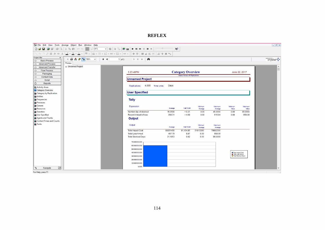
114
REFLEX

115
AUTHOR’S BIOGRAPHY
Gustav Albertzeth received his undergraduate
degree in Logistics and Supply Chain Management
from Industrial Engineering Department of
Universitas Atma Jaya Yogyakarta (UAJY) in 2013
by completing his Final Assignment (T.A)
“Application of Particle Swarm Optimization on
Capacitated Team Orienteering Problem”. In 2015
decided to pursue a Master Program on Operations
and Supply Chain Engineering (OSCE) in
Industrial Engineering Department of Institut
Teknologi Sepuluh Nopember Surabaya. During
the completion of the Master Program for 2 years (4 semesters), he decided to
continuing his area of research since the undergraduate level which is transportation
in supply chain, by completing his Thesis “Cost-Effective Strategy to Mitigate
Transportation Disruption in Supply Chain”. Author can be reached by email:
.

116
This page is intentionally left blank