Costs and Benefits of Dynamic Trading in a Lemons

Market

William Fuchs∗ Andrzej Skrzypacz

May 8, 2013

Abstract

We study a dynamic market with asymmetric information that creates the lemons

problem. We compare effi ciency of the market under different assumptions about the

timing of trade. We identify positive and negative aspects of dynamic trading, describe

the optimal market design under regularity conditions and show that continuous-time

trading can be always improved upon.

1 Introduction

Consider liquidity-constrained owners who would like to sell assets to raise capital for prof-

itable new opportunities. Adverse selection, as in Akerlof (1970), means that if owners have

private information about value trade will be ineffi cient, even in competitive markets. In

this paper we show how that ineffi ciency is affected by market design in terms of when the

sellers can trade.

In Akerlof (1970) the seller makes only one decision: to sell the asset or not. However, in

practice, if the seller does not sell immediately, there are often future opportunities to trade.

Delayed trade can be used by the market as a screen to separate low value assets (those that

sellers are more eager to sell) from high-value assets. As we show in this paper, dynamic

trading creates costs and benefits for overall market effi ciency. On the positive side, the

∗Fuchs: Haas School of Business, University of California Berkeley (e-mail: wfuchs@haas.berkeley.edu).Skrzypacz: Graduate School of Business, Stanford University (e-mail: skrz@stanford.edu). We thank IlanKremer, Mikhail Panov, Christine Parlour, Aniko Öry, Brett Green, Marina Halac, Johanna He, Alessan-dro Pavan, Felipe Varas, Robert Wilson, and participants of seminars and conferences for comments andsuggestions.

1

screening via costly delay increases in some instances overall liquidity of the market: more

types eventually trade in a dynamic trading market than in the static/restricted trading

market. On the negative side, future opportunities to trade reduce the amount of early

trade, making the adverse selection problem worse. There are two related reasons. First,

keeping the time 0 price fixed, after a seller decides to reject it, buyers update positively

about the value of the asset and hence the future price is higher. That makes it desirable

for some seller types to wait. Second, the types who wait are a better-than-average selection

of the types were supposed to trade at time 0 in a static model and hence this additional

adverse selection reduces p0. In turn, even more types wait, reducing effi ciency further.

We study different ways of designing the market in terms of picking the times when the

market opens. For example, we compare effi ciency of a continuously opened market to a

design in which the seller can trade only once at t = 0 and otherwise has to wait until the

type is revealed at some T (we allow the asymmetric information to be short-lived, T <∞,as well as fully persistent, T =∞).1

We motivate our analysis by an example with linear valuations (the value to buyers is a

linear function of the seller value) and uniform distribution of seller types. We show that the

market with restricted trading opportunities (allowing trades only at t = 0 and at T ) is on

average more effi cient than a market with continuous-time trading. In fact, for large T the

deadweight loss caused by adverse selection is three times as large if continuous trading is

allowed. It may appear that preventing costly screening/signaling could always be welfare-

improving as in the education signaling models (Spence 1973). Via a different example we

show that this is not always true: since in a market for lemons immediate effi cient trade is

not possible, in some situations screening via costly delay can help welfare.

Our main result (Theorem 1) shows that we can always improve upon a continuous trading

market design. In particular, we show that introducing a "lock-up" period, that is allowing

the seller to trade at t = 0 and then closing the market for some (small) time window,

followed by continuous trading, is welfare improving. Said differently, there always exist

restrictions on trading opportunities that improve welfare.

Under some fairly standard regularity conditions we can significantly strengthen our result.

In Theorem 2 we show that making the “lock up” last from immediately after the first

opportunity to trade until the time information arrives (or never allowing trade again if no

information ever arrives) generates higher expected gains from trade than any other market

timing design not just the continuous trading benchmark.

1In Section 6.2 we consider information arriving at random time.

2

For both of these results, and the recommended policy implications, it is of course im-

portant to be able to identify in practice what time zero in the model corresponds to. Our

model shares this issue with any model in which time on the market plays a signaling role.

In practice, identifying the time the gains from trade arise (say, because the seller is hit by

a liquidity need) might not always be easy. Certain occasions might nonetheless provide a

good proxy. For example, in a widespread financial crises, capital requirements are likely to

become binding for several financial institutions and this is often publicly observed. Merril

et. al (2013) show that the willingness to sell residential mortgage backed securities by insur-

ance companies can be partly explained by the severity with which their capital constraints

were binding. Another example is that firms that enter into bankruptcy commonly divest

non-core assets and could use costly delay to signal the value of those assets. For such situ-

ations, our model suggests that to maximize expected gains from trade there should be an

organized auction early in the bankruptcy process and that creditors might want to subsidize

trades that take place in this auction and dissuade future opportunities to trade these assets.

Our findings that restrictions to future trading improve welfare bring up an important

practical issue: can the involved parties credibly commit to keeping the market closed in the

future. As we point out in Remark 2, one way to achieve such commitment is to make trades

completely anonymous, so that past buyers could re-sale the asset if the market becomes

active without their counterparties knowing whether they are facing the original seller or a

previous buyer. If this is implemented then buyers would be discouraged to purchase the

asset after time zero since they would face additional adverse selection. As a result, the

seller would not be able to get a higher price if he delays transaction (unless he waits till the

information arrives) and the gains from trade we describe in this paper would be realized.

We then consider an alternative design: what if market is opened continuously until some

time interval before information arrives? We show that this design has qualitatively different

consequences than the "lock-up" period in which market is closed after the initial trade

opportunity at t = 0. The reason is that closing the market before T creates an additional

endogenous market closure. If the last opportunity to trade before T is at t∗, in equilibrium

there is an additional time interval (t∗∗, t∗) such that nobody trades even though trades are

allowed. The intuition is that failing to trade at t∗ implies a strictly positive delay cost for

the seller and as a result an atom of types trades at t∗. That reduction in adverse selection

allows the buyers to offer a good price. In turn, waiting for this good price makes the adverse

selection right before t∗ so extreme that the market freezes. This additional delay cost can

completely undo the effi ciency gains that accrue at t∗ - we argue that such short closures

have a very small impact on total welfare and that the overall effect can be either positive

3

or negative.

Next we discuss how our findings can be applied to inform government policy. When infor-

mation frictions get really bad, the government may consider a direct intervention (beyond

trying to regulate the dynamic trading). We have seen several of these interventions during

the recent financial crisis. For example, the government could guarantee a certain value of

traded assets (this was done with the debt issues by several companies and as part of some

of the takeover deals of financially distressed banks). Alternatively, the government could

directly purchase some of the assets (for example, real estate loan portfolios from banks as

has been done in Ireland and is being discussed as a remedy for the Spanish banking crisis).

We point out an important equilibrium effect that seems to be absent of many public

discussions about such government bailouts. It is not just the banks that participate in the

asset buyback or debt guarantee programs that benefit from the government’s intervention.

The whole financial sector benefits because liquidity is restored to markets. As a result,

non-lemons manage to realize higher gains from trade thanks to the intervention. We relate

our findings to the recent work by Philippon and Skreta (2012) and Tirole (2012). We

argue that unlike in their static-market analysis, the government can improve welfare by a

comprehensive intervention which involves not only assets buy-backs but also restricts the

post-intervention private markets. Finally, we point out that expectation of an asset buy-

back (or any other intervention that leads to an atom of types trading) in the near term may

drastically reduce liquidity as in the "late closure" market design, partially undermining the

benefits of that intervention.

1.1 Related Literature

Our paper is related to literature on dynamic markets with adverse selection. The closest

paper is Janssen and Roy (2002) who study competitive equilibria in a market that opens

at a fixed frequency (and long-lived private information, T = ∞). In equilibrium prices

increase over time and eventually every type trades. They point out that the outcome is still

ineffi cient even as per-period discounting disappears (which is equivalent to taking a limit

to continuous trading in our model) since trade suffers from delay costs even in the limit.

They do not ask market design questions as we do in this paper (for example, what is the

optimal frequency of opening the market). Yet, we share with their model the observation

that dynamic trading with T = ∞ leads to more and more types trading over time. For

other papers on dynamic signaling/screening with a competitive market see Noldeke and

van Damme (1990), Swinkels (1999), Kremer and Skrzypacz (2007) and Daley and Green

4

(2011). While we share with these papers an interest in dynamic markets with asymmetric

information, none of these papers focuses on market design questions.

From the mechanism-design perspective, a closely related paper is Samuelson (1984). It

characterizes a welfare-maximizing mechanism in the static model subject to no-subsidy

constraints. When T = ∞, this static mechanism design is mathematically equivalent to

a dynamic mechanism design since choosing probabilities of trade is analogous to choosing

delay. Therefore our proof of Theorem 2 uses the same methods as Samuelson (1984).

As we mentioned already, our paper is also related to Philippon and Skreta (2012) and

Tirole (2012) who study mechanism design (i.e. government interventions) in the presence

of a market ("competitive fringe"). Our focus is on a different element of market design, but

we also discuss how these two approaches can be combined.

Our analysis can be described as "design of timing" in the sense that we compare equilib-

rium outcomes for markets/games that differ in terms of the time when players move. That

is related in spirit to Damiano, Li and Suen (2012), who study optimal delay in committee

decisions where the underlying game resembles a war of attrition.

A different design question for dynamic markets with asymmetric information is asked in

Hörner and Vieille (2009), Kaya and Liu (2012), Kim (2012) and Fuchs, Öry and Skrzypacz

(2012). These papers take the timing of the market as given (a fixed frequency) and ask

how information about past rejected offers affects effi ciency of trade. It is different from our

observation in Remark 2 since this is about observability of accepted rather than rejected

offers.2

Finally, there is also a recent literature on adverse selection with correlated values in

models with search frictions (among others, Guerrieri, Shimer and Wright (2010), Guerrieri

and Shimer (2011) and Chang (2012)). Rather than having just one market in which different

quality sellers sell at different times, the separation of types in these models is achieved

because market differ in market tightness with the property that in a market with low prices

a seller can find a buyer very quickly and in a market with high prices it takes a long time to

find a buyer. Low-quality sellers which are more eager to sell quickly self-select into the low

price market while high quality sellers are happy to wait longer in the high price market. One

can relate our design questions to a search setting by studying the effi ciency consequences of

closing certain markets (for example, using a price ceiling). This would roughly correspond

to closing the market after some time in our setting.

2Moreno and Wooders (2012) ask a yet another design question: they compare decentralized searchmarkets with centralized competitive markets.

5

2 The Model

As in the classic market for lemons, a potential seller owns one unit of an indivisible asset.

When the seller holds the asset, it generates for him a revenue stream with net present

value c ∈ [0, 1] that is private information of the seller. The seller’s type, c, is drawn from

a distribution F (c) , which is common knowledge, atomless and has a continuous, strictly

positive density f (c). At time T ≤ ∞ the seller’s type is publicly revealed.3

There is a competitive market of potential buyers. Each buyer values the asset at v (c)

which is strictly increasing, twice continuously differentiable, and satisfies v (c) > c for all

c < 1 (i.e. common knowledge of gains from trade) and v (1) = 1 (i.e. no gap on the top).

These assumptions imply that in the static Akerlof (1970) problem some but not all types

trade in equilibrium.4

Time is t ∈ [0,∞] and we consider different market designs in which the market is opened

in different moments in that interval. We start the analysis with two extreme market designs:

"infrequent trading" (or "restricted trading") in which the market is opened only twice at

t ∈ 0, T and "continuous trading" in which the market is opened in all t ∈ [0, T ] . Note

that the first time the market opens after the private information is revealed trade will take

place immediately with probability 1. Let Ω ⊆ [0, T ] denote the set of times that the market

is open (we assume that at the very least 0, T ⊂ Ω, but see Section 6.3 for the possibility

of restricting trade also at and after T ).

Every time the market is open, there is a market price at which buyers are willing to trade

and the seller either accepts it (which ends the game) or rejects. If the price is rejected the

game moves to the next time the market is opened. If no trade takes place by time T the

type of the seller is revealed and the price in the market is v (c), at which all seller types

trade.

All players discount payoffs at a rate r and we let δ = e−rT . If trade happens at time t at

a price pt, the seller’s payoff is (1− e−rt

)c+ e−rtpt

and the buyer’s payoff is

e−rt (v (c)− pt)

A competitive equilibrium is a pair of functions pt, kt for t ∈ Ω where pt is the market

3We could think of the public revelation of the banking stress tests as a possible example of this.4Assuming v (1) = 1 allows us not to worry about out-of-equilibrium beliefs after a history where all seller

types are supposed to trade but trade did not take place. We discuss this assumption further in Section 6.4.

6

price at time t and kt is the highest type of the seller that trades at time t.5 These functions

satisfy:

(1) Zero profit condition: pt = E [v (c) |c ∈ [kt−, kt]] where kt− is the cutoff type at the

previous time the market is open before t (with kt− = 0 for the first time the market is

opened.)6

(2) Seller optimality: given the process of prices, each seller type maximizes profits by

trading according to the rule kt.7

(3) Market Clearing: in any period the market is open, the price is at least pt ≥ v (kt−) .

Conditions (1) and (2) are standard. Condition (3) deserves a bit of explanation. We

justify it by a market clearing reasoning, that demand equals supply given the prices. In

particular, suppose the asset was offered at a price pt < v (kt−) at time t. Then, since all

buyers believe that the value of the good is at least v (kt−) , they would all demand it.

Demand could not be equal to supply, the market could not clear. This condition removes

some trivial multiplicity of equilibria. For example, it removes as a candidate equilibrium a

path (pt, kt) = (0, 0) for all periods (i.e. no trade and very low prices) even though this path

satisfies the first two conditions.8

We assume that all market participants publicly observe all the trades. Hence, once a

buyer obtains the asset, if he tries to put it back on the market, the market makes a correct

inference about c based on the history. Since we assume that all buyers have the same value

of the asset, there would not be any profitable re-trading of the asset (after the initial seller

transacts) and hence we ignore that possibility (however, see Remark 2).

3 Motivating Example and Benchmark Trading De-

signs

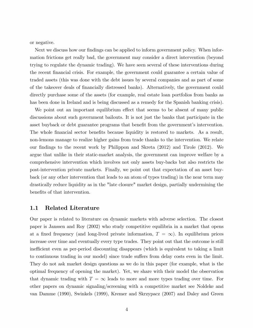
Before we present the general analysis of the problem, consider the following example. As-

sume c is distributed uniformly over [0, 1] and v (c) = 1+c2, as illustrated in Figure 1.

5Since we know that the skimming property holds in this environment it is simpler to directly define thecompetitive equilibrium in terms of cutoffs.

6In continuous time we use a convention kt− = lims↑t ks, E [v (c) |c ∈ [kt−, kt]] =lims↑tE [v (c) |c ∈ [ks, kt]] , and v (kt−) = lims↑t v (ks) . If kt = kt− then the condition is pt = v (kt) .

7Implicitly, we require that the price process is such that an optimal seller strategy exists.8Condition (3) is analogous to the condition (iv) in Janssen and Roy (2002) and is weaker than the No

Unrealized Deals condition in Daley and Green (2011) (see Definition 2.1 there; since they study the gapcase, they need a stronger condition to account for out-of-equilibrium beliefs).

7

0.0 0.2 0.4 0.6 0.8 1.00.0

0.5

1.0

c

v(c)

gains

from tra

de

Figure 1: Gains from trade in the benchmark example.

We compare two possible market designs. First, infrequent trading, that is ΩI = 0, T .Second, continuous trading, ΩC = [0, T ] .

Remark 1 In this paper we analyze competitive equilibria. In this benchmark example it ispossible to write a game-theoretic version of the model allowing two buyers to make public

offers every time the market is open. If we write the model having Ω = 0,∆, 2∆, ..., Tthen we can show that there is a unique Perfect Bayesian Equilibrium for every T and

∆ > 0. When ∆ = T then the equilibrium coincides with the equilibrium in the infrequent

trading market we identify below. Moreover, taking the sequence of equilibria as ∆ → 0,

the equilibrium path converges to the competitive equilibrium we identify for the continuous

trading design. In other words, the equilibria we describe in this section have a game-theoretic

foundation.

Infrequent Trading The infrequent trading market design corresponds to the classic mar-

ket for lemons as in Akerlof (1970). The equilibrium in this case is described by a price p0

and a cutoff k0 that satisfy that the cutoff type is indifferent between trading at t = 0 and

waiting till T :

p0 = (1− δ) k0 + δ1 + k0

2

and that the buyers break even on average:

p0 = E [v (c) |c ≤ k0]

The solution is k0 = 2−2δ3−2δ

and p0 = 4−3δ6−4δ

. The expected gains from trade are

SI =

∫ k0

0

(v (c)− c) dc+ δ

∫ 1

k0

(v (c)− c) dc =4δ2 − 11δ + 8

4 (2δ − 3)2

8

With infrequent trading, ΩI , for general f and v we have the following characterization of

equilibria:9

Proposition 1 (Infrequent/Restricted Trading) For ΩI = 0, T there exists a com-petitive equilibrium p0, k0 . Equilibria are a solution to:

p0 = E [v (c) |c ∈ [0, k0]] (1)

p0 =(1− e−rT

)k0 + e−rTv (k0) (2)

If f(c)F (c)

(v (c)− c)− δ1−δv

′ (c) is strictly decreasing, the equilibrium is unique.

Continuous Trading The above outcome cannot be sustained in equilibrium if there are

multiple occasions to trade before T. If at t = 0 types below k0 trade, the next time the

market opens price would be at least v (k0) . If so, types close to k0 would be strictly better

off delaying trade. As a result, for any set Ω richer than ΩI , in equilibrium there is less trade

in period 0.

If we look at the case of continuous trading, ΩC = [0, T ] , then the equilibrium with

continuous trade is a pair of two processes pt, kt that satisfy:

pt = v (kt)

r (pt − kt) = pt

The intuition is as follows. Since the process kt is continuous, the zero profit condition is

that the price is equal to the value of the current cutoff type. The second condition is the

indifference of the current cutoff type between trading now and waiting for a dt and trading

at a higher price. These conditions yield a differential equation for the cutoff type

r (v (kt)− kt) = v′ (kt) kt

with the boundary condition k0 = 0. In our example it has a simple solution:

kt = 1− e−rt.9The infrequent trading model is the same as the model in Akerlof (1970) if T =∞. All proofs are in the

Appendix.

9

The total surplus from continuous trading is

SC =

∫ T

0

e−rt (v (kt)− kt) ktdt+ e−rT∫ 1

kT

(v (c)− c) dc =1

12

(2 + δ3

).

For general f and v, with continuous trading opportunities ΩC , the equilibrium is unique:

Proposition 2 (Continuous trading) For ΩC = [0, T ] a competitive equilibrium (unique

up to measure zero of times) is the unique solution to:

pt = v (kt)

k0 = 0

r (v (kt)− kt) = v′ (kt) kt (3)

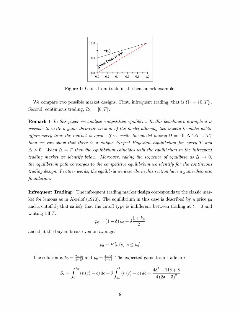
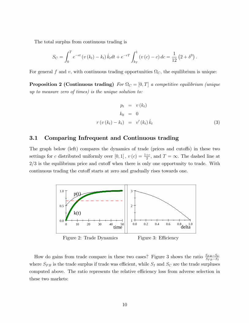
3.1 Comparing Infrequent and Continuous trading

The graph below (left) compares the dynamics of trade (prices and cutoffs) in these two

settings for c distributed uniformly over [0, 1] , v (c) = 1+c2, and T = ∞. The dashed line at

2/3 is the equilibrium price and cutoff when there is only one opportunity to trade. With

continuous trading the cutoff starts at zero and gradually rises towards one.

0 10 20 30 40 500.0

0.5

1.0

time

k(t)

p(t)

Figure 2: Trade Dynamics

0.0 0.2 0.4 0.6 0.8 1.01

2

3

delta

Figure 3: Effi ciency

How do gains from trade compare in these two cases? Figure 3 shows the ratio SFB−SCSFB−SI

where SFB is the trade surplus if trade was effi cient, while SI and SC are the trade surpluses

computed above. The ratio represents the relative effi ciency loss from adverse selection in

these two markets:

10

• When δ → 0 (i.e. as rT →∞, the private information is long-lived) we getSFB−SCSFB−SI → 3

so the effi ciency loss with continuous trading is three times higher than with infrequent

trading.

• When δ → 1 (i.e. T → 0 so the private information is very short-lived), the organi-

zation of the market does not matter since even by waiting till T players can achieve

close to full effi ciency in either case.

What affects relative effi ciency of the two market designs? The trade-off is as follows.

Committing to only one opportunity to trade generates a big loss of surplus if players do not

reach an agreement in the current period. This clearly leaves a lot of unrealized gains from

trade. But it is this ineffi ciency upon disagreement that helps overcome the adverse selection

problem and increases the amount of trade in the initial period. Continuous trading on the

other hand does not provide many incentives to trade in the current period since a seller

suffers a negligible loss of surplus from delay. This leads to an equilibrium with smooth

trading over time. While the screening of types via delay is costly, the advantage is that

eventually (if T is large enough) more types trade. In determining which trading environment

is more effi cient on average, one has to weight the cost of delaying trade with low types with

the advantage of eventually trading with more types.

3.1.1 Can Continuous Trading be Better?

Our example above demonstrates a case of v (c) and F (c) such that for every T the infrequent

trading market is more effi cient than the continuous trading market. Furthermore, the

greater the T , the greater the effi ciency gains from using infrequent trading. Is it a general

phenomenon? The answer is no:

Proposition 3 There exist v (c) and F (c) such that for T large enough the continuous

trading market generates more gains from trade than the infrequent trading market

The example used in the proof of this proposition illustrates what could make the contin-

uous trading market to dominate the infrequent one: we need a large mass at the bottom

of the distribution, so that the infrequent trading market gets "stuck" with only these types

trading, while under continuous trading these types trade quickly, so the delay costs for these

types are small. Additionally, we need some mass of higher types that would be reached

in the continuous trading market after some time, generating additional surplus. Alterna-

tively, one can construct examples in which the gains from trade are small for low types

11

and get large for intermediate types, so that some delay cost at the beginning is more than

compensated by the increased overall probability of trade.

4 Optimality of Restricting Trading Opportunities

4.1 General Market Designs

So far we have compared only the continuous trading market with the infrequent trading.

But one can imagine many other ways to organize the market. For example, the market

could clear every day; or every ∆ ∈ (0, T ) . Or the market could be opened at 0, then closed

for some time interval ∆ and then be opened continuously. Or, the market could start being

opened continuously and close some ∆ before T (i.e. at t = T − ∆). In this section we

consider some of these alternative designs.

4.1.1 Closing the Market Briefly after Initial Trade.

Our main result follows. We show that continuous-trading market is never an optimal design.

In particular, consider the design ΩEC ≡ 0 ∪ [∆, T ]: trade is allowed at t = 0, then the

market is closed till ∆ > 0 and then it is opened continuously till T. We call this design

"early closure". We show that one can always find ∆ > 0 that improves upon continuous

trading:

Theorem 1 For every r, T, F (c) , and v (c) , there exists ∆ > 0 such that the early closure

market design ΩEC = 0∪ [∆, T ] yields higher gains from trade than the continuous trading

design ΩC = [0, T ].

To establish that early closure increases effi ciency of trade we show in the proof an even

stronger result: that for small ∆ with ΩEC there is more trade overall and all types that

trade trade sooner, so social surplus is higher type-by-type. Let kEC∆ be the highest type

that trades at t = 0 when the design is ΩEC . Let kC∆ the equilibrium cutoff at time ∆ in

design ΩC . We establish this stronger claim by showing that for small ∆, kC∆ < kEC∆ . Since

with ΩEC once the market re-opens at ∆ the equilibrium is the same as in case of ΩC but

with the different boundary condition, the claim follows.

The proof proceeds by showing that:

lim∆→0

∂kEC∆

∂∆= 2 lim

∆→0

∂kC∆∂∆

.

12

Since as ∆→ 0 both kEC∆ and kC∆ converge to 0, this means that for small ∆ approximately

twice as many types trade before ∆ if the market is closed than if it is opened in (0,∆) .

The intuition is as follows. When we close the market for some time, some types that were

planning to trade in (0,∆) now would prefer to trade at 0 even if the price at 0 does not

change. The reason is that not taking the price p0 implies a fixed delay cost. It turns out

that the set of types that decide to take that fixed p0 grows approximately as fast in ∆ as

does kC∆.

That early closure doubles early trade is then acheived because pooling of trade at time

0 reduces the adverse selection that buyers face and hence price p0 increases. For small ∆

the price is approximately half way between v (0) and v(kEC∆

)(since we assumed that f (c)

and v (c) are positive and continuous, we can use the linear-uniform approximation as in

the example in Section 3). As the price goes up, even more types prefer to trade at 0 and

the adverse selection problem is reduced even further, making p0 even higher, and so on.

Becasue prices grow at half the speed of v(kC∆), the kEC∆ is twice as high as kC∆.

4.1.2 When Infrequent Trading is Optimal

We showed above that it is never optimal to have the market continuously open. Namely, a

small closure of the market after the initial opportunity to trade generates an improvement

over continuously open markets. If a small closure generates an improvement, what a about

a larger one? We show next that although there are exceptions, as illustrated in Proposition

3, we can find a relatively general set of conditions under which indeed the optimal thing

is to have infrequent trading ΩI = 0, T . In fact, our result is that for a large class ofenvironments design ΩI dominates not only ΩC but any other Ω : closing the market at all

intermediate periods is better than any other timing protocol not just continuous trading.

A suffi cent condition for our result is:

Definition 1 We say that the environment is regular if f(c)F (c)

v(c)−c1−δ+δv′(c) and

f(c)F (c)

(v (c)− c) aredecreasing.

A suffi cient condition is that v′′ (c) ≥ 0 and f(c)F (c)

(v (c)− c) is decreasing. This regularitycondition is similar to the standard condition in optimal auction theory/pricing theory that

the virtual valuation/marginal revenue curve be monotone. In particular, think about a

static problem of a monopsonist buyer choosing a cutoff (or a probability to trade, F (c)),

by making a take-it-or-leave-it offer equal to P (c) = (1− δ) c + δv (c) . In that problemf(c)F (c)

v(c)−c1−δ+δv′(c) decreasing guarantees that the marginal profit crosses zero exactly once.

10

10The FOC of the monopolist problem choosing c is: (1− δ) f (c) (v (c)− c)−F (c) ((1− δ) + δv′ (c)) = 0.

13

Theorem 2 If the environment is regular then infrequent trading, ΩI = 0, T , generateshigher expected gains from trade than any other market design.

Our proof considers a relaxed mechanism design problem with a market maker who max-

imizes expected gains from trade. The designer is allowed to cross-subsidize buyers trading

in different periods (other than at T ) but has to break even (only) on average.11. We show

that the regularity condition is suffi cient for the solution to the relaxed problem to be that

types below a threshold trade immediately and types above the threshold wait till T, with

no trade in the middle. That solution to the relaxed problem can be implemented by a

competitive equilibrium and hence ΩI design is the most effi cient (in case design ΩI leads to

multiple equilibria, our theorem applies to the one in which the threshold k0 is the highest).

If the solution to the relaxed problem does not have the property that all trade happens

only at t = 0 or t = T, then it involves the cross-subsidization of the buyers and the allocation

of the relaxed mechanism cannot be implemented as a competitive equilibrium without the

use of taxes and subsidies. It is an open question how to solve for the optimal Ω if the

solution to the relaxed problem calls for trade in more than one period. The diffi culty is

that the constraints on the mechanism are then endogenous. A mechanism that calls for a

set of types to trade at time t has to have a price equal to the average v (c) across these

types. Hence, as Ω changes (or the range of the allocation function changes), the set of

constraints changes as well.

Commitment to Infrequent Trading Although, as we have shown above, it might be

optimal to commit to having just a unique trading opportunity ex-post (after time 0) there is

an incentive to trade again immediately rather than waiting all the way until time T. Hence

an important practical question is if indeed these trading restrictions can be implemented

or not. If indeed there was no commitment power and no credible way of stopping parties

from trading, then sellers and buyers would recognize this and the equilibrium would be the

one with continuous trading opportunities that we know is ineffi cient. From a market design

perspective this paper highlights that it is important to try to figure out credible ways in

which to restrict trading opportunities.

In the following Remark we propose Extreme Anonymity of the market as one possible

Also note if F (c) is log-concave then f(c)F (c) is decreasing.

11For T = ∞, this is a problem analyzed in Samuelson (1984). Our contribution is that we analyze ageneral T and provide suffi cient conditions for the solution to have no trade in (0, T ) . Also, he studiesprobability of trade in a static mechanism design and we look at the timing of trade in a dynamic settingalbeit these two problems are tightly connected.

14

way in which we might organize information to achieve an effective market closure even in

the case in which the market cannot be physically closed.

Remark 2 One way to implement ΩI = 0, T in practice may be via an Extreme Anonymityof the market. In our model we have assumed that the initial seller of the asset can be told

apart in the market from buyers who later become secondary sellers. However, if the trades

are completely anonymous, even if Ω 6= 0, T , the equilibrium outcome would coincide with

the outcome for ΩI . The reason is that the price can never go up since otherwise the early

buyers of the low-quality assets would resell them at the later markets.

Such extreme anonymity may not be feasible in some markets (for example, IPO’s), or not

practical for reasons outside the model. Yet, it may be feasible in some situations. For exam-

ple, a government as a part of an intervention aimed at improving effi ciency of the market

may create a trade platform in which it would act as a broker who anonymizes trades and

traders.

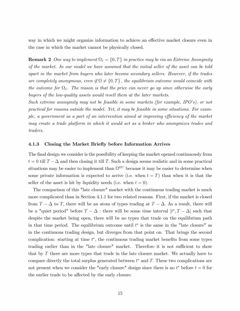
4.1.3 Closing the Market Briefly before Information Arrives

The final design we consider is the possibility of keeping the market opened continuously from

t = 0 till T −∆ and then closing it till T. Such a design seems realistic and in some practical

situations may be easier to implement than ΩEC because it may be easier to determine when

some private information is expected to arrive (i.e. when t = T ) than when it is that the

seller of the asset is hit by liquidity needs (i.e. when t = 0).

The comparison of this "late closure" market with the continuous trading market is much

more complicated than in Section 4.1.1 for two related reasons. First, if the market is closed

from T − ∆ to T, there will be an atom of types trading at T − ∆. As a result, there will

be a "quiet period" before T − ∆ : there will be some time interval [t∗, T −∆] such that

despite the market being open, there will be no types that trade on the equilibrium path

in that time period. The equilibrium outcome until t∗ is the same in the "late closure" as

in the continuous trading design, but diverges from that point on. That brings the second

complication: starting at time t∗, the continuous trading market benefits from some types

trading earlier than in the "late closure" market. Therefore it is not suffi cient to show

that by T there are more types that trade in the late closure market. We actually have to

compare directly the total surplus generated between t∗ and T. These two complications are

not present when we consider the "early closure" design since there is no t∗ before t = 0 for

the earlier trade to be affected by the early closure.

15

The equilibrium in the "late closure" design is as follows. Let p∗T−∆, k∗T−∆ and t∗ be a

solution to the following system of equations:

E [v (c) |c ∈ [kt∗ , kT−∆]] = pT−∆ (4)(1− e−r∆

)kT−∆ + e−r∆v (kT−∆) = pT−∆ (5)(

1− e−r(T−∆−t∗)) kt∗ + e−r(T−∆−t∗)pT−∆ = v (kt∗) (6)

where the first equation is the zero-profit condition at t = T − ∆, the second equation is

the indifference condition for the highest type trading at T −∆ and the last equation is the

indifference condition of the lowest type that reaches T −∆, who chooses between trading

at t∗ and at T −∆. The equilibrium for the late closure market is then:

1) at times t ∈ [0, t∗] , (pt, kt) are the same as in the continuous trading market

2) at times t ∈ (t∗, T −∆), (pt, kt) = (v (kt∗) , kt∗)

3) at t = T −∆, (pt, kt) =(p∗T−∆, k

∗T−∆

)Condition (6) guarantees that given the constant price at times t ∈ (t∗, T −∆) it is indeed

optimal for the seller not to trade. There are other equilibria that differ from this equilibrium

in terms of the prices in the "quiet period" time: any price process that satisfies in this time

period (1− e−r(T−∆−t)) kt∗ + e−r(T−∆−t)pT−∆ ≥ pt ≥ v (kt∗)

satisfies all our equilibrium conditions. Yet, all these paths yield the same equilibrium

outcome in terms of trade and surplus (of course, the system (4) − (6) may have multiple

solutions that would have different equilibrium outcomes).

Despite this countervailing ineffi ciency, for our leading example:

Proposition 4 Suppose v (c) = 1+c2and F (c) = c. For every r and T there exists a ∆ > 0

such that the "late closure" market design, ΩLC = [0, T −∆]∪T , generates higher expectedgains from trade than the continuous trading market, ΩC. Yet, the gains from late closure

are smaller than the gains from early closure.

The proof (in the Appendix) shows third-order gains of welfare from the late closure, while

the gains from early closure are first-order. Figure 4 below illustrates the reason the gains

from closing the market are smaller relative to when the market is closed at time zero. The

bottom two lines show the evolution of the cutoff type in ΩC (continuous curve) and in ΩLC

(discontinuous at t = T −∆ = 0.9). The top two lines show the corresponding path of prices.

The gains from bringing forward trades that occur when the market is exogenously closed in

16

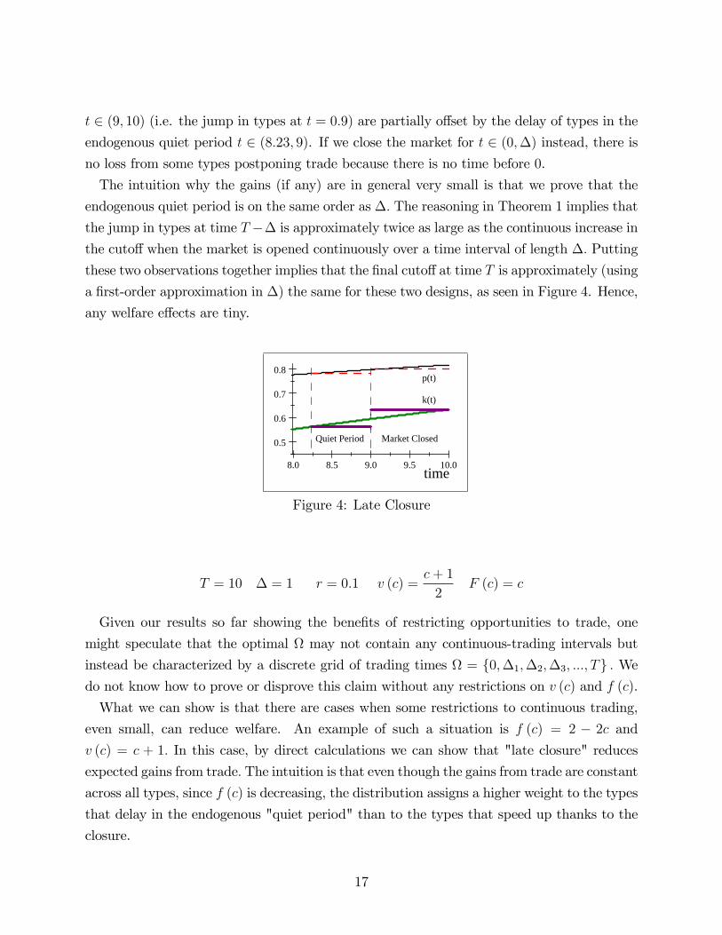
t ∈ (9, 10) (i.e. the jump in types at t = 0.9) are partially offset by the delay of types in the

endogenous quiet period t ∈ (8.23, 9). If we close the market for t ∈ (0,∆) instead, there is

no loss from some types postponing trade because there is no time before 0.

The intuition why the gains (if any) are in general very small is that we prove that the

endogenous quiet period is on the same order as ∆. The reasoning in Theorem 1 implies that

the jump in types at time T −∆ is approximately twice as large as the continuous increase in

the cutoff when the market is opened continuously over a time interval of length ∆. Putting

these two observations together implies that the final cutoffat time T is approximately (using

a first-order approximation in ∆) the same for these two designs, as seen in Figure 4. Hence,

any welfare effects are tiny.

8.0 8.5 9.0 9.5 10.0

0.5

0.6

0.7

0.8

time

k(t)

p(t)

Market ClosedQuiet Period

Figure 4: Late Closure

T = 10 ∆ = 1 r = 0.1 v (c) =c+ 1

2F (c) = c

Given our results so far showing the benefits of restricting opportunities to trade, one

might speculate that the optimal Ω may not contain any continuous-trading intervals but

instead be characterized by a discrete grid of trading times Ω = 0,∆1,∆2,∆3, ..., T . Wedo not know how to prove or disprove this claim without any restrictions on v (c) and f (c).

What we can show is that there are cases when some restrictions to continuous trading,

even small, can reduce welfare. An example of such a situation is f (c) = 2 − 2c and

v (c) = c + 1. In this case, by direct calculations we can show that "late closure" reduces

expected gains from trade. The intuition is that even though the gains from trade are constant

across all types, since f (c) is decreasing, the distribution assigns a higher weight to the types

that delay in the endogenous "quiet period" than to the types that speed up thanks to the

closure.

17

5 Implications for Asset Purchases by the Government

Market failure due to information frictions sometimes calls for government intervention.

During the recent financial crisis several markets effectively shut down or became extremely

illiquid. One of the main reasons cited for this was the realization by market players that

the portfolios of asset backed securities that banks held were not all investment grade as

initially thought. Potential buyers of these securities which used to trade them without much

concern suddenly became very apprehensive of purchasing these assets for the potential risk

of buying a lemon. The Treasury and the Federal Reserve tried many different things to

restore liquidity into the markets. Some of the measures were aimed at providing protection

against downside risk via guarantees effectively decreasing the adverse selection problem

or by removing the most toxic assets from the banks’balance sheets (for example, via the

TARP I and II programs or central banks’acceptance of toxic assets as collateral).

Our model provides a natural framework to study the potential role for government. To

illustrate consider the case in which if v (c) = γc for 2 > γ > 1 and F (c) = c.12 Then for all

Ω the unique equilibrium is for there never to be any trade before the information is revealed.

So the market is completely illiquid and no gains from trade are realized. The government

could intervene in this market by making an offer pg > 0 to buy any asset sellers are willing

to sell at that price (these programs are by and large voluntary).

In this example, the average quality of these assets will be pg2and hence the government

would lose money on them. On the bright side is that once the toxic assets have been

removed from the market and the remaining distribution is truncated to c ∈[pgγ, 1]now

even if Ω = [0+, T ] buyers would be willing to start making offers again.

We want to make two observations about this intervention. First, in the post-intervention,

continuously-opened market the liquidity is characterized by (3) which in this example sim-

plifies to:

rktγ − 1

γ= kt

Therefore, the larger the initial intervention, the faster the trade in the free market af-

terwards. Second, this government intervention benefits not only the direct recipients of

government funds but also all other sellers since by reducing the adverse selection problem

in the market they will now have an opportunity trade with a private counterparty.

Optimal government interventions in very similar (though richer) models have been studied

12This model arises for example if the seller has a higher discount rate than the buyers.

18

recently by Philippon and Skreta (2012) and Tirole (2012). In these papers the government

offers financing to firms having an investment opportunity and it is secured by assets that

the firms have private information about. That intervention is followed by a static com-

petitive market in which firms that did not receive funds from the government can trade

privately. This creates a problem of "mechanism design with a competitive fringe" as named

by Philippon and Skreta (2012).

The setup in these two papers can be roughly mapped to ours if we assume v (c)−c = γ.13

Our paper directly applies to section II (Buybacks only) in Tirole (2012), but we believe

that the following observations apply more broadly.

Both papers show that the total surplus cannot be improved by the government shutting

down private markets: see Proposition 2 in Tirole (2012) and Theorem 2 in Philippon and

Skreta (2012). Since the post-intervention market creates endogenous IR constraints for

the agents participating in the government program, making it less attractive could make it

easier for the government to intervene. However, these two papers argue that this is never a

good idea.

Our results show that taking into account the dynamic nature of the market changes

this conclusion. In particular, the assumptions in Tirole (2012) satisfy the assumptions in

Theorem 2 (he assumes f(c)F (c)

is decreasing). Therefore it would be optimal for the government

to concentrate post-intervention trades to be right after it and commit to shutting down the

market afterwards. This could be achieved by organizing a market at t = 0, offering a subsidy

to trades and announcing that all trades afterwards will be taxed. Alternatively, offering

(partial) insurance for assets traded at a particular time window but not later. Finally,

creating an anonymous exchange (see Remark 2) may be a practical solution.

Additionally, our analysis of the late closure suggests that if the market expects the govern-

ment may run a program of that nature in near future, the market may close endogenously,

even if trade would continue if no such intervention were expected. The reasoning is the

same: if a non-trivial fraction of seller types participate in the government transaction, the

post-intervention price is going to be strictly higher than the current cutoff’s v (kt) and hence

there are no trades that could be profitable for both sides.

13In both papers there is an additional restriction that the seller needs to raise a minimal amount of moneyto make a profitable investment, which is the source of gains from trade. That additional aspect does notchange our conclusions.

19

6 Discussion

In this section we explore a few extensions of the model.

6.1 High Frequency Trading

High frequency trading has recently receives increased attention by both policy makers and

researchers.14 Large investments are being made by market participants to have access to

information about trades in other exchanges a few miliseconds before other players. Our

model abstracts from many potentially important institutional details but the Corrollary to

Theorem 1 discussed below would seem to indicate that it might be optimal to regulate speed

by potentially putting a lower bound on the frequency with which the market is open. Within

out setting one can think of high frequency trading as a situation in which the informational

asymmetries are very short lived, i.e. T small. We hope to address this question in more

detail in future research.

Corollary 1 For every r, v (c) , and F (c) there exists a T ∗ > 0 such that for all T ≤ T ∗

the infrequent trading market design generates higher expected gains from trade than the

continuous trading design.

The proof is analogous to the proof of the Theorem 1 by noting that in either situation:

ΩEC = 0∪ [∆, T ] or ΩI = 0, T = ∆ the cutoff type trading at time 0 chooses between p0

and price v (k0) . In case information is revealed at T this is by assumption that the market

is competitive at T. In case the market is open continuously after the early closure it is by

our observation that the continuation equilibrium has smooth screening of types so the first

price after closure is p∆ = v(kEC∆

).

6.2 Stochastic Arrival of Information

So far we have assumed that it is known that the private information is revealed at T. How-

ever, in some markets, even if the private information is short-lived, the market participants

may be uncertain about the timing of its revelation.

To capture that idea we have analyzed a version of our model in which there is no fixed

time T information is revealed, so that Ω ⊆ [0,∞] , but over time, with a constant Poisson

rate λ exogenous information arrives that publicly reveals the seller’s type. We assume that

for any Ω, once the information arrives trade is immediate at price p = v (c) .

14See for example Pagnotta and Philippon (2012)

20

The following results can be established for this model:

1. If Ω = [0,∞] then for all λ the equilibrium is as described in Proposition 2.

2. Theorem 1 holds.

3. If f(c)F (c)

v(c)−cλv′(c)+r is decreasing then the analog of Theorem 2 holds (i.e., with this new

condition replacing the regularity condition, fully restricting trade between t = 0 and

the time information is revealed maximizes total surplus.

The proofs of these claims are analogous to the proofs in the original and hence are

omitted (but they are available from the authors upon request). The intuition why the

equilibrium path of prices and cutoffs before information arrives is the same in the stochastic

and deterministic arrival of information cases is as follows. In the deterministic case, the

benefit of delaying trade by dt is that the price increases by ptdt. In the stochastic case, the

price also increases, but additionally with probability λdt the news arrives. If so, the current

cutoff type gets a price v (kt) instead of pt+dt. However, since pt = v (kt) , price pt+dt is only

of order dt higher than what the current cutoff gets upon arrival. Therefore, the additional

effect of delaying trade is a term on the order of dt2 and so with continuous trading it does

not affect incentives to delay, and so the equilibrium path of cutoffs is unchanged.

To illustrate the model with random arrival, return to our benchmark example with v (c) =1+c

2and F (c) = c. In the infrequent trading market, the equilibrium (p0, k0) is determined

by:

p0 =λ

λ+ rv (k0) +

r

λ+ rk0

p0 = E [v (c) |c ≤ k0]

where the first equation is the indifference condition of the cutoff type and the second

equation is the usual zero-profit condition. In our example we get

k0 =2r

3r + λ, p0 =

4r + λ

6r + 2λ

We now can compare the gains from trade. The total gains from trade in the infrequent

trading market are:

SI =

∫ k0

0

(v (c)− c) dc+λ

λ+ r

∫ 1

k0

(v (c)− c) dc.

21

In the continuous trading market (since the path of types is the same as we computed

before) the gains are:

SC =

∫ +∞

0

λe−λt(∫ kt

0

e−rτ(c) (v (c)− c) dc+ e−rt∫ 1

kt

(v (c)− c) dc)dt

where τ (c) = − ln(1−c)r

is the time type c trades if there is no arrival before τ (c) . Direct

calculations yield:

S0 (z)− SC (z) =1

2(z + 3)−2 > 0

where z ≡ λr. So, for every λ, the infrequent trading market is more effi cient than the

continuous trading market, consistent with the analog of Theorem 2.

6.3 Beyond Design of Ω : Affecting T

In this paper we analyze different choices of Ω. A natural question is what else could a

market designer affect to improve the market effi ciency. One such possibility is information

structure, as we have discussed in Remark 2. There are of course other options for changing

information (for example, should past rejected offers be observed or not?), but that is beyond

the scope of this paper.

Another possibility is affecting T. Clearly, if the market designer could make T very small,

it would be good for welfare since it would make the market imperfections short-lived. That

may not be feasible though. Suppose instead that the designer could only increase T (for

example, by making some verification take longer).15 Surprisingly, it turns out that in some

cases increasing T could improve effi ciency. While it is never beneficial in the continuous-

trading case (since it does not affect trade before T and only delays subsequent trades), it

can help in other cases. To illustrate it, Figure 5 graphs the expected gains from trade in our

leading example for ΩI = 0, T as a function of δ. It turns out that if and only if e−rT < 12,

increasing T is welfare improving.

15We thank Marina Halac for suggesting this question.

22

0.0 0.2 0.4 0.6 0.8 1.00.21

0.22

0.23

0.24

0.25

delta

S

Figure 5: Surplus with infrequent

trading as a function of T

6.4 Common Knowledge of Gains from Trade

We have assumed that v (0) > 0 and v (1) = 1, that is, strictly positive gains from trade for

the lowest type and no gains on the top. Can we relax these assumptions?

6.4.1 Role of v (0) > 0

If v (0) = 0 then Theorem 2 still applies. As we argued above, if the market is opened

continuously, in equilibrium there is no trade before T (to see this note that the starting

price would leave the lowest type with no surplus, so that type would always prefer to wait for

a price increase). That does not need to be true for other Ω. For example, if v (c) =√c and

F (c) = c, then for all T the conditions in Theorem 2 are satisfied. Therefore, ΩI = 0, T iswelfare-maximizing and ΩC = [0, T ] is welfare-minimizing over all Ω; and if δ < 2

3then the

ranking is strict since there is some trade with ΩI .

6.4.2 Role of v (1) = 1

The main reason we assume v (1) = 1 is that in this way we do not need to define equilibrium

market prices after histories where the seller trades with probability 1. That is, when v (1) =

1, the highest type never trades in equilibrium no matter how large is T . This makes our

definition of competitive equilibrium simpler than in Daley and Green (2011) (compare our

condition (3) "Market Clearing" with Definition 2.1 there).

To illustrate how the freedom in selecting off-equilibrium-path beliefs can lead to a mul-

tiplicity of equilibria with radically different outcomes consider the following heuristic rea-

23

soning. Assume:

F (c) = c ; v (c) = c+ s

Suppose that Ω = 0,∆, 2∆, ..., T for ∆ > 0. Let s > 12so that in a static problem trade

would be effi cient.

Case 1: Assume that when an offer that all types accept on the equilibrium path is

rejected, buyers believe the seller has the highest type, c = 1. That is, post-rejection price

is 1 + s. Then, taking a sequence of equilibria as ∆→ 0, we can show that in the limit trade

is smooth over time (no atoms) with:

pt(k) = v (kt)

kt = rst

On equilibrium path all types trade by:

τ =1

rs

unless τ < T. If the last offer, pτ = 1 + s is rejected, the price stays constant after that,

consistently with the beliefs and competition.

Case 2: Alternatively, assume that when an offer that all types accept on the equilibriumpath is rejected, buyers do not update their beliefs. That is, after that history they believe

the seller type is distributed uniformly over [kt, 1] , where kt is derived from the history of the

game. In that case we can construct the following equilibrium for all ∆ > 0. At t = 0 there

is an initial offer p0 = 12

+ s and all types trade. If that initial offer is rejected, the buyers

believe c˜U [0, 1] and continue to offer pt = p0 for all t > 0 (and again all types trade). This

is indeed and equilibrium since the buyers break even at time zero (and at all future times

given their beliefs) and no seller type is better off by rejecting the initial offer.

These equilibria are radically different in terms of effi ciency: only the second one is effi -

cient. It is beyond the scope of this paper to study in what situations or under what model

extensions this multiplicity could be resolved and how. v (1) > 1 creates similar problems

for large T even if immediate effi cient trade is not possible. On the other hand, if the gap on

top is small so that for a given T in equilibrium it is not possible that all types trade before

T, then our analysis still applies.

24

7 Conclusions

In this paper we have analyzed a dynamic market with asymmetric information. Our two

main results are that, first, under mild regularity conditions restricting trade to ΩI = 0, Tdominates any other design. Second, even more generally, effi ciency can be improved over

continuous-time trading by the "early closure" design which after initial auction restricts

additional trading for some interval of time. We discussed how these findings can inform

government policy geared towards resolving market failures due to the lemons problem.

Unlike the previous papers using a static model of the market, we argue that an intervention

would be more successful if the government could at least partially restrict dynamic trading

after the intervention. The bottom line is that we have identified a non-trivial cost to

dynamic trading: it makes the adverse selection problem worse.

Many open questions remain. On a more technical note, it is an open question how to

compute the optimal Ω if our regularity conditions do not hold. On a more practical note,

in many markets the time the game actually starts is ill-defined and/or sellers arrive to the

market at different times (as opposed to a whole market being hit by liquidity shocks as in

the recent financial crisis). Even in the case of IPOs it is not clear how to define the first

time the market considers the owners of the startup to delay an offering with the hope of

affecting investors’beliefs (i.e. at which point signaling via delay starts). Moreover, one

may be interested in embedding this model into a larger market with many sellers hit by

liquidity needs at different times to gain additional insights about market design. Janssen

and Karamychev (2002) show that equilibria in dynamic markets with dynamic entry can be

qualitatively different from markets with one-time entry if the "time on the market" is not

observed by the market (see also Hendel, Lizzeri and Siniscalchi 2005 and Kim 2012 about

the role of observability of past transaction/time on the market). As pointed out recently

by Roy (2012), a dynamic market can suffer from an additional ineffi ciency if buyers are

heterogeneous because the high valuation buyers are more eager to trade sooner and it

may be that they are the effi cient buyers of the high quality goods. Incorporating these

considerations into our design questions may introduce new tradeoffs.

Finally, in our model there were only two sources of signaling: delay and the exogenous

signal that arrives only once. In many markets sellers may want to wait for multiple pieces

of news to arrive over time before they agree to sell (as in Daley and Green 2011), and a

market designer may try to influence both the timing of possible trades and the timing of

information release.

25

8 Appendix

Proof of Proposition 1. 1) Existence. The equilibrium conditions follow from the

definition of equilibrium. To see that there exists at least one solution to (1) and (2) note

that if we write the condition for the cutoff as:

E [v (c) |c ≤ k0]−((

1− e−rT)k0 + e−rTv (k0)

)= 0 (7)

then the LHS is continuous in k0, it is positive at k0 = 0 and negative at k0 = 1. So there

exists at least one solution. 16

2) Uniqueness. To see that there is a unique solution under the two assumptions, notethat the derivative of the LHS of (7) at any k is

f (k)

F (k)(v (k)− E [v (c) |c ≤ k])− (1− δ)− δv′ (k)

When we evaluate it at points where (7) holds, the derivative is

f (k)

F (k)(v (k)− k) (1− δ)− (1− δ)− δv′ (k)

and that is by assumption decreasing in k.

Suppose that there are at least two solutions and select two: the lowest kL and second-

lowest kH . Since kL is the lowest solution, at that point the curve on the LHS of (7)must have

a weakly negative slope (since the curve crosses zero from above). However, our assumption

implies that curve has even strictly more negative slope at kH . That leads to a contradiction

since by assumption between [kL, kH ] the LHS is negative, so with this ranking of derivatives

it cannot become 0 at kH

Proof of Proposition 2. First note that our requirement pt ≥ v (kt−) implies that there

cannot be any atoms of trade, i.e. that kt has to be continuous. Suppose not, that at time

s types [ks−, ks] trade with ks− < ks. Then at time s + ε the price would be at least v (ks)

while at s the price would be strictly smaller to satisfy the zero-profit condition. But then

for small ε types close to ks would be better off not trading at s, a contradiction. Therefore

we are left with processes such that kt is continuous and pt = v (kt) . For kt to be strictly

16If there are multiple solutions, a game theoretic-model would refine some of them, see section 13.B ofMas-Colell, Whinston and Green (1995) for a discussion.

26

increasing over time we need that r (pt − kt) = pt for almost all t: if price was rising faster,

current cutoffs would like to wait, a contradiction. If prices were rising slower over any time

interval starting at s, there would be an atom of types trading at s, another contradiction.

So the only remaining possibility is that pt, kt are constant over some interval [s1, s2] . Since

the price at s1 is v(ks1−

)and the price at s2 is v (ks2) , we would obtain a contradiction that

there is no atom of trade in equilibrium. In particular, if ps1 = ps2 (which holds if and only

if ks1− = ks1 = ks2) then there exist types k > ks1 such that

v (ks1) >(1− er(s2−s1)

)k + er(s2−s1)v (ks1)

and these types would strictly prefer to trade at t = s1 than to wait till s2, a contradiction

again.

Proof of Proposition 3. Consider a distribution that approximates the following: with

probability ε c is drawn uniformly on [0, 1] ; with probability α (1− ε) it is uniform on [0, ε] ;

and with probability (1− α) (1− ε) it is uniform on [c1, c1 + ε] for some c1 > v (0) . In other

words, the mass is concentrated around 0 and c1. Let v (c) = 1+c2as in our example.

For small ε there exists α < 1 such that

E [v (c) |c ≤ c1 + ε] < c1

so that in the infrequent trading market trade will happen only with the low types. In

particular, if α is such that

αv (0) + (1− α) v (c1) < c1

then as ε → 0 and T → ∞, the infrequent trading equilibrium price converges to v (0) and

the surplus converges to

limε→0,T→∞

SI = αv (0) + (1− α) c1

The equilibrium path for the continuous trading market is independent of the distribution

and hence

limε→0,T→∞

SC = αv (0) + (1− α)[e−rτ(c1)v (c1) +

(1− e−rτ(c1)

)c1

]= lim

ε→0,T→∞SI + (1− α)

(e−rτ(c1) (v (c1)− c1)

)where τ (k) is the inverse of the function kt. The last term is strictly positive for any c1 <

27

v (c1) . In particular, with v (c) = 1+c2, e−rτ(c) = (1− c) and v (c1)− c1 = 1

2(1− c1) , so

limε→0,T→∞

SC = limε→0,T→∞

SI +1

2(1− α) (1− c1)2 .

Proof of Theorem 1. To establish that early closure increases effi ciency of trade we show

an even stronger result: that for small ∆ with ΩEC there is more trade at t = 0 than with

ΩC by t = ∆. Let kEC∆ be the highest type that trades at t = 0 when the design is ΩEC . Let

kC∆ the equilibrium cutoff at time ∆ in design ΩC . Then the stronger claim is that for small

∆, kC∆ < kEC∆ . Since lim∆→0 kEC∆ = lim∆→0 k

C∆ = 0 (for kEC∆ see discussion in Step 1 below),

it is suffi cient for us to rank:

lim∆→0

∂kEC∆

∂∆vs. lim

∆→0

∂kC∆∂∆

Step 1: Characterizing lim∆→0∂kEC∆

∂∆.

Consider ΩEC . When the market reopens at t = ∆ the market is continuously open from

then on. Hence, the equilibrium in the continuation game is the same as the equilibrium

characterized in Proposition 2 albeit with a different starting lowest type. Namely, for t ≥ ∆

pt = v (kt)

r (v (kt)− kt) = v′ (kt) kt

with a boundary condition:

k∆ = kEC∆ .

The break even condition for buyers at t = 0 implies:

p0 = E[v (k) |k ∈

[0, kEC∆

]]and type kEC∆ must be indifferent between trading at this price at t = 0 or for p∆ = v

(kEC∆

)at t = ∆ :

v(kEC∆

)− p0 =

(1− e−r∆

) (v(kEC∆

)− kEC∆

)So kEC∆ is the solution to:

v(kEC∆

)− E

[v (k) |k ∈

[0, kEC∆

]]=(1− e−r∆

) (v(kEC∆

)− kEC∆

)(8)

28

Using implicit function theorem we can show that:

lim∆→0

∂kEC∆

∂∆=

2rv (0)

v′ (0)

Intuitively, for small ∆, E[v (c) |c ≤ kEC∆

]≈ v(0)+v(kEC∆ )

2(because we have assumed that

f (c) and v (c) are positive and continuous). so the benefit of waiting, the left-hand side

of (8) , is approximatelyv(kEC∆ )−v(0)

2while the cost of waiting, the right-hand side of (8) , is

approximately r∆v (0) so kEC∆ for small ∆ solves approximately

v(kEC∆

)− v (0)

2= r∆v (0)

which yields ∂kEC∆

∂∆= 2rv(0)

v′(0)as ∆→ 0.

Step 2: Characterizing lim∆→0∂kC∆∂∆.

Consider ΩC . Since kt is defined by the differential equation

r (v (kt)− kt) = v′ (kt) kt,

for small ∆ :

kC∆ ≈ r∆v (0)

v′ (0),

and more precisely:

lim∆→0

∂kC∆∂∆

=rv (0)

v′ (0).

Summing up steps 1 and 2, we have:

lim∆→0

∂kEC∆

∂∆= 2 lim

∆→0

∂kC∆∂∆

which implies the claim.

Proof of Theorem 2. We use mechanism design to establish the result. Consider the

following relaxed problem. There is a mechanism designer who chooses a direct revelation

mechanism that maps reports of the seller to a probability distribution over times he trades

and to transfers from the buyers to the mechanism designer and from the designer to the

seller. The constraints on the mechanism are: incentive compatibility for the seller (to report

truthfully); individual rationality for the seller and buyers (the seller prefers to participate

in the mechanism rather than wait till T and get v (c) and the buyers do not lose money on

29

average); and that the mechanism designer does not lose money on average. Additionally,

we require that the highest type, c = 1, does not trade until T (as in any equilibrium he

does not).

For every game with a fixed Ω, the equilibrium outcome can be replicated by such a

mechanism, but not necessarily vice versa, since if the mechanism calls for the designer

cross-subsidizing buyers across periods, it cannot be replicated by a competitive equilibrium.

Within this class of direct mechanisms we characterize one that maximizes ex-ante ex-

pected gains from trade. We then show that is the environment is regular, infrequent trading

replicates the outcome of the best mechanism and hence any other market design generates

lower expected gains from trade.

A general direct revelation mechanism can be described by 3 functions x (c) , y (c) and

P (c) , where y (c) is the probability that the seller will not trade before information is

released, x (c) is the discounted probability of trade over all possible trading times and P (c)

is the transfer received by the seller conditional on trading before information is released.17

Note that y (c) ∈ [0, 1] but x (c) ∈ [δ, 1] .

The seller’s value function in the mechanism is:

U (c) = y (c) [(1− δ) c+ δv (c)] + (1− y (c)) [P (c) + (1− x (c)) c] (9)

= maxc′

y (c′) [(1− δ) c+ δv (c)] + (1− y (c′)) [P (c′) + (1− x (c′)) c] (10)

Using the envelope theorem:18

U ′ (c) = y (c) [(1− δ) + δv′ (c)] + (1− y (c)) (1− x (c))

= δy (c) (v′ (c)− 1) + 1− x (c) (1− y (c))

Let V (c) = δv (c) + (1− δ) c be the no-trade surplus, so:

U ′ (c)− V ′ (c) = δy (c) (v′ (c)− 1) + 1− x (c) (1− y (c))− (δv′ (c) + (1− δ))= (1− y (c)) (−x (c)− δ (v′ (c)− 1))

17Letting Gt (c) denote for a given type the distribution function over the times of trade:

x (c) =

∫ T

0

e−rtdGt (c) .

18This derivative exists almost everywhere and hence we can use the integral-form of the envelope formula,(11) .

30

As a result, we can write the expected seller’s gains from trade as a function of the allocations

x (c) and y (c) only:

S =

∫ 1

0

(U (c)− V (c)) f (c) dc

= (U (c)− V (c))F (c) |c=1c=0 −

∫ 1

0

(U ′ (c)− V ′ (c))F (c) dc

=

∫ 1

0

(1− y (c)) [x (c)− δ (1− v′ (c))]F (c) dc (11)

Clearly, the mechanism designer will leave the buyers with no surplus (since he could use it

to increase effi ciency of trade) and so maximizing S is the designer’s objective. That also

means that the no-losses-on-average constraint is:∫ 1

0

(1− y (c)) (x (c) v (c)− P (c)) f (c) dc ≥ 0

From the expression for U (c) we have

U (c)− y (c) [(1− δ) c+ δv (c)]− (1− y (c)) (1− x (c)) c = (1− y (c))P (c)

U (c)− V (c) + (1− y (c)) (δ (v (c)− c) + x (c) c) = (1− y (c))P (c)

So the constraint can be re-written as a function of the allocations alone (where the last

term expands as in (11)):∫ 1

0

(1− y (c)) (x (c)− δ) (v (c)− c) f (c) dc−∫ 1

0

(U (c)− V (c)) f (c) dc ≥ 0 (12)

We now optimize (11) subject to (12) , ignoring necessary monotonicity constraints on

x (c) and y (c) that assure that reporting c truthfully is incentive compatible (we check later

that they are satisfied in the solution).

The derivatives of the Lagrangian with respect to x (c) and y (c) are:

Lx (c) = (1− y (c)) [F (c) + Λ ((v (c)− c) f (c)− F (c))]

−Ly (c) = (x (c)− δ (1− v′ (c)))F (c) + Λ [(x (c)− δ) (v (c)− c) f (c)− (x (c)− δ (1− v′ (c)))F (c)]

where Λ > 0 is the Largrange multiplier.

Consider Lx (c) first. Note that [F (c) + Λ ((v (c)− c) f (c)− F (c))] is positive for c = 0.

31

Suppose f(c)F (c)

(v (c)− c) is decreasing (which is part of the regularity assumption). Let c∗ bethe unique solution to 1 − f(c)

F (c)(v (c)− c) = 1

Λ(if it exists, otherwise, let c∗ = 1). If c∗ < 1

then the second term in Lx (c) changes sign once at c∗. An optimal x (c) is therefore:

x (c) =

1 if c ≤ c∗

δ if c > c∗

Now consider −Ly (c) . For all c ≤ c∗, using the optimal x (c) , it simplifies to:

−Ly (c) = (1− δ + δv′ (c))F (c)+Λ [(1− δ) (v (c)− c) f (c)− (1− δ + δv′ (c))F (c)] for x (c) = 1

If f(c)F (c)

v(c)−c1+ δ

(1−δ)v′(c)

is decreasing in c, (which is part of the regularity assumption), Ly (c)

changes sign once in this range. It is negative for c ≤ c∗∗ and positive for c > c∗∗, where

c∗∗ ≤ c∗ is a solution to f(c)F (c)

(v (c)− c) =(1− 1

Λ

) (1 + δ

(1−δ)v′ (c)). Therefore the optimal

y (c) in this range is

y (c) =

0 if c ≤ c∗∗

1 if c > c∗∗

For c > c∗, using the optimal x (c) , the derivative Ly (c) simplifies to

Ly (c) = − (1− Λ) δv′ (c)F (c) for x (c) = δ

If Λ > 1, this is positive and the optimal y (c) is equal to 1. If Λ ≤ 1, c∗ = 1 and hence this

case would be empty.

That finishes the description of the optimal allocations in the relaxed problem: there

exists a c∗ such that types below c∗ trade immediately and types above it wait till after

information is revealed at T. The higher the c∗ the higher the gains from trade. The largest

c∗ that satisfies the constraint is the largest solution of:

E [v (c) |c ≤ c∗] = (1− δ) c∗ + δv (c∗)

since the LHS is the IR constraint of the buyers and the RHS is the IR constraint of the c∗

seller. This is also the equilibrium condition in a market with design Ω = 0, T , so thatequilibrium implements the solution to the relaxed problem.

Proof of Proposition 4.

32

In this case the equilibrium conditions (4) , (5) and (6) simplify to

1

2+kt∗ + kT−∆

4= pT−∆ (6′)(

1− e−r∆)kT−∆ +

(1

2+kT−∆

2

)e−r∆ = pT−∆ (7′)(

1− e−r∆2)kt∗ + e−r∆2pT−∆ =

1

2+kt∗

2(8′)

where ∆2 = T −∆− t∗.Solution of the first two equations is:

kT−∆ =kt∗ + 2− 2e−r∆

3− 2e−r∆

pT−∆ =1

2

(2− e−r∆3− 2e−r∆

kt∗ +4− 3e−r∆

3− 2e−r∆

)Substituting the price to the last condition yields

(1− e−r∆2

)kt∗ + e−r∆2

(1

2

(2− e−r∆3− 2e−r∆

kt∗ +4− 3e−r∆

3− 2e−r∆

))=

1

2+kt∗

2

which can be solved for ∆2 independently of kt∗ (given our assumptions about v (c) and

F (c)).

r∆2 = − ln3− 2e−r∆

4− 3e−r∆

Note that

lim∆→0

∂∆2

∂∆= lim

∆→0

∂

∂∆

1

r

(− ln

3− 2e−r∆

4− 3e−r∆

)= 1

so ∆2 is approximately equal to ∆.

In the continuous trading cutoffs follow kt = 1 − e−rt, kt = re−rt. Normalize T = 1 (and

rescale r appropriately). Then

kt∗ = 1− e−r(1−∆−∆2) = 1− 4− 3e−r∆

3− 2e−r∆er∆δ

where δ = e−r and

t∗ = 1−∆−∆2 = 1−∆ +1

rln

3− 2e−r∆

4− 3e−r∆

We can now compare gains from trade in the two cases. The surplus starting at time t∗ is

33

(including discounting):

Sc (∆) =

∫ 1−e−r

kt∗

e−rτ(c) (v (c)− c) dc+ δ

∫ 1

1−e−r(v (c)− c) dc

=

∫ 1−e−r

kt∗

(1− c)(

1− c2

)dc+ δ

∫ 1

1−e−r

(1− c

2

)dc

where we used e−rτ(c) = 1− c.

∂Sc (∆)

∂∆= −∂kt

∗

∂∆

(1− kt∗)2

2

and since lim∆→0∂kt∗∂∆

= −2rδ we get that

lim∆→0

∂Sc (∆)

∂∆= rδ3

For the "late closure" market the gains from trade are

SLC (∆) = e−r(1−∆)

∫ kT−∆

kt∗

(v (c)− c) dc+ e−r∫ 1

kT−∆

(v (c)− c) dc

after substituting the computed values for kt∗ and kT−∆ it can be verified that

lim∆→0

∂SLC (∆)

∂∆= rδ3

which is the same as in the case of continuous market, so to the first approximation even

conditional on reaching t∗ the gains from trade are approximately the same in the two market

designs.

We can compare the second derivatives:

lim∆→0

∂S2LC (∆)

∂∆2= 3δ3r2

lim∆→0

∂S2c (∆)

∂∆2= 3δ3r2

34

and even these are the same. Finally, comparing third derivatives:

lim∆→0

∂S3LC (∆)

∂∆3= 13r3δ3

lim∆→0

∂S3c (∆)

∂∆3= 9r3δ3

so we get that for small ∆, the "late closure" market generates slightly higher expected

surplus, but the effects are really small.

References

[1] Akerlof, George. A. (1970). "The Market for "Lemons": Quality Uncertainty and the

Market Mechanism." Quarterly Journal of Economics, 84 (3), pp. 488-500.

[2] Chang (2012). "Adverse Selection and Liquidity Distortion in Decentralized Markets."

Northwestern Mimeo.

[3] Daley, Brendan and Brett Green (2011) "Waiting for News in the Market for Lemons."

forthcoming in Econometrica.

[4] Damiano, Ettore, Li, Hao and Wing Suen (2012) "Optimal Delay in Committees."

Working paper.

[5] Fuchs, William, Aniko Öry and Andrzej Skrzypacz (2012) "Transparency and Distressed

Sales under Asymmetric Information." UC Berkeley, Mimeo.

[6] Guerrieri, Veronica, Robert Shimer, and Randall Wright (2010) "Adverse Selection in

Competitive Search Equilibrium." Econometrica, 78 (6), pp. 1823-1862.

[7] Guerrieri, Veronica and Robert Shimer (2012) "Dynamic Adverse Selection: A Theory

of Illiquidity, Fire Sales, and Flight to Quality.", working paper.

[8] Hendel, Igal, Alessandro Lizzeri, and Marciano Siniscalchi (2005) "Effi cient Sorting in

a Dynamic Adverse-Selection Model." Review of Economic Studies 72 (2), 467-497.

[9] Hörner, Johannes and Nicolas Vieille (2009) "Public vs. Private Offers in the Market

for Lemons." Econometrica, 77 (1), pp. 29-69.

[10] Janssen, Maarten C. W. and Vladimir A. Karamychev (2002) "Cycles and multiple

equilibria in the market for durable lemons," Economic Theory, 20 (3), pp. 579-601.

35

[11] Janssen, Maarten C. W. and Santanu Roy (2002) "Dynamic Trading in a Durable

Good Market With Asymmetric Information." International Economic Review, 43 (1),

pp. 257-282.

[12] Kaya, Ayca and Liu, Qingmin (2012) "Transparency and Price Formation," working

paper.

[13] Kremer, Ilan and Andrzej Skrzypacz (2007) "Dynamic Signaling and Market Break-

down." Journal of Economic Theory, 133 (1), pp. 58-82.

[14] Kim, Kyungmin (2012) "Information about Sellers’Past Behavior in the Market for

Lemons," working paper.

[15] Mas-Colell, Andreu; Michael D. Whinston and Jerry R. Green (1995). Microeconomic

Theory. New York: Oxford University Press.

[16] Moreno, Diego and John Wooders (2012). "Dynamic Markets for Lemons: Performance,

Liquidity, and Policy Intervention," University Carlos III de Madrid Working paper 12-

26.

[17] Nöldeke, Georg and Eric van Damme (1990) "Signalling in a Dynamic Labour Market."

Review of Economic Studies, 57 (1), pp. 1-23.

[18] Pagnotta, Emiliano and Philippon, Thomas (2012) Competing on Speed

(April 27, 2012). Available at SSRN: http://ssrn.com/abstract=1967156 or

http://dx.doi.org/10.2139/ssrn.1967156.

[19] Philippon, Thomas and Skreta, Vasiliki (2012) "Optimal Interventions in Markets with

Adverse Selection", American Economic Review, 102 (1), pp. 1-28.

[20] Roy, Santanu (2012) "Dynamic Sorting in Durable Goods Markets with Buyer Hetero-

geneity," working paper.

[21] Samuelson, William (1984) "Bargaining under Asymmetric Information." Econometrica,

52 (4), pp. 995-1005.

[22] Spence, A.M. (1973) "Job Market Signaling.", Quarterly. Journal of Economics, 87, pp.

355-374.

[23] Swinkels, Jeroen M. (1992) "Educational Signalling With Preemptive Offers." Review

of Economic Studies, 66 (4), pp. 949-970.

36

[24] Tirole, Jean (2012) "Overcoming Adverse Selection: How Public Intervention Can Re-

store Market Functioning." American Economic Review, 102 pp. 19-59.

37