costs of financial distress and capital structure of …
TRANSCRIPT

COSTS OF FINANCIAL DISTRESS AND CAPITAL STRUCTURE OF FIRMS
AYDIN OZKAN
Thesis presented for the degree of D.PHIL
UNIVERSITY OF YORK
DEPARTMENT OF ECONOMICS AND RELATED STUDIES
March 1996

Pages
iv
V
Vi
vii
viii
CONTENTS
Acknowledgements
Declaration
Abstract
List of Tables
List of Figures
Chapter 1 Introduction
Chapter 2 A Survey on Capital Structure Theories
2.1 Introduction
2.2 Modigliani and Miller Analysis
2.3 Bankruptcy Costs and Tax Savings
2.4 Personal and Corporate Taxation
2.5 Agency Costs
2.6 Asymmetric Information and Signalling Approach
2.7 Sources of Finance and Bargaining-based Theories of
Corporate Finance
2.8 Conclusions
Chapter 3 Investment Incentives of Financially Distressed Firms
3.1 Introduction
3.2 The Model
3.2.1 Strategies in Period T
3.2.2 Strategies in Period T-1
3.2.3 Strategies in Period t
3.3 Conclusions
Chapter 4 Corporate Bankruptcies and the Role of Banks
4.1 Introduction
4.2 The Model
1
10
11
12
15
24
27
31
33
36
43
44
48
56
59
63
66
68
69
73
1

4.2.1 Strategy of Firm 2
78
4.2.2 Strategy of the Bank
81
4.2.3 Strategy of Firm 1
89
4.2.4 Determination of Debt Reduction Ratio 91
4.3 Generalisation of the Basic Model
93
4.3.1 Strategy of Firm 1
93
4.3.2 Strategy of the Bank
94
4.4 Conclusions
97
Chapter 5 Economics of Insolvency Procedures and Inefficient Company
Liquidations
99
5.1 Introduction 100
5.2 The Role of Bankruptcy Law and Existing UK Procedures
102
5.2.1 The Role of Bankruptcy Law 102
5.2.2 The UK Insolvency Procedures 103
5.2.2.1 Liquidation
103
5.2.2.2 Receivership 104
5.2.2.3 Administration 105
5.2.2.4 Company Voluntary Arrangements (CVA's) 105
5.3 Economic Analysis of UK Insolvency Procedures and Asset
Structure of Firms 106
5.3.1 The Model
107
5.3.2 Equilibrium of the Game
111
5.3.3 Discussion 117
5.4 Conclusions
119
Chapter 6 A Model of Capital Structure Theory
121
6.1 Introduction
122
6.2 Optimal Capital Structure Theories
123
6.2.1 Single-period Model
123
6.2.2 Multi-period Model
125
6.3 The Model
127
6.3.1 The Market Value of Equity 131
li

181
182
183
185
187
188
6.3.2 The Market Value of Debt
134
6.3.3 The Market Value of the Firm 136
6.3.4 The Optimal Capital Structure 137
6.3.5 Comparative Statics 139
6.4 Conclusions 144
Chapter 7 Empirical Evidence on the Capital Structure of Firms 147
7.1 Introduction 148
7.2 Determinants of Capital Structure 150
7.2.1 Size 150
7.2.2 Growth Opportunities 151
7.2.3 Non-debt Tax Shields
152
7.2.4 Profitability 152
7.2.5 Liquidity 153
7.2.6 Operating Leverage
154
7.3 Empirical Model and Data 154
7.3.1 Empirical Model
154
7.3.2 Data
159
7.4 Empirical Results
160
7.5 Conclusions
170
Chapter 8 Conclusions
Appendices
Appendix 6.1 Leibnit'z Rule
Appendix 6.2 Derivation of c3QIäI
Appendix 6.3 Derivation of the Optimality Condition; aviai
Appendix 6.4 Derivation of 32 V/I 8R
Appendix 7.1 Data
References
173
193
111

ACKNOWLEDGEMENTS
I wish to express my gratitude to Dr. Sandeep Bhargava for his supervision and
encouragement during the preparation of this thesis. I am also grateful to Prof. Peter
Simmons and Peter C. Smith for the helpful discussions and comments they have made on
the various drafts of this study. I am also glad to acknowledge the advice and support of
Prof. John Hey.
I am also indebted to Etibank for their generous financial support during my post-
graduate studies.
I should also thank my parents for their patience. Their understanding and support
have been invaluable.
Finally, many thanks to Gulcin, my wife, for her loving support during the
preparation of this thesis. It would not be possible to complete this study without her help
and support.
lv
DECLARATION
A version of Chapter 4 was presented at the Young Economists session of the
Money, Macro and Finance Group Annual Conference, September 1995, at Cardiff
Business School. It has been selected to be published in The Manchester School of
Economic and Social Studies, June 1996 Conference issue. A version of this chapter has
also appeared as a discussion paper (Department of Economics Discussion Paper, No.
95/32, University of York, 1995).
A version of Chapter 5 was published in The METU Studies in Development, 1995,
Vol.22, No.4, pp.425-439. It has also been circulated as a discussion paper. (Department
of Economics Discussion Paper, No. 95/31, University of York, 1995).
Chapters 3 and 7 have been circulated as discussion papers (Department of
Economics Discussion Paper, No. 96/26 and 96/27, University of York, 1996).
v

ABSTRACT
The main purpose of this study is to explore the iiteractions between costly financial
distress and capital structure of firms. The topic of capital structure has been a subject of
investigation in finance since the seminal studies of Modigliani and Miller (1958, 1963).
Their second work implied that in a world with corporate taxes a firm's capital structure
would consist of almost a 100 percent of debt. This extreme implication has led
researchers to look for explanations to fill the gap between the M-M prediction and
observed capital structure of firms. The topic of bankruptcy and financial distress gained
a great deal of attention as a result of these attempts. However, there has not been a
consensus neither on the role nor on their significance in the determination of a firm's
capital structure. Therefore this thesis attempts to provide more insight into the
understanding of the interaction between these costs and corporate financial policy. In
order to explore this interaction this study focuses on two types of costs which are related
to financial distress. First, there are costs that arise from distortionary incentives and
conflicting interests of various agents of the firm. Second, there are also costs which are
due to the decrease in the firm value in liquidation. This study argues that when there is
asymmetric information between shareholders and bondholders about the true financial
condition of the firm, shareholders may deviate from value maximising decisions in
financial distress at the expense of bondholders. It is also shown that individualistic
behaviour of creditors leads to premature and inefficient liquidations of firms which
experience financial distress temporarily and have continuation values greater than their
liquidation values. In deriving these implications liquidation costs and the impact of the
firm's asset characteristics on these costs constitute the central elements of this study. This
thesis also sheds light on the importance of firm size in the insolvency process. It is argued
that small firms are more likely to be liquidated than large firms when they are in financial
distress. The findings of the empirical analysis of this study are in line with this view. The
empirical results of a UK company panel data analysis also reveal that profitability, growth
opportunities and liquidity conditions of firms are important determinants of borrowing
decisions of companies.
vi

LIST OF TABLES
Table 2.1 Capital Structure Theories and Empirical Results 38
Table 3.1 Payoffs to Shareholders and Bondholders of Firms 51
Table 4.1 Payoffs to an Insolvent Firm and a Bank Which Can
be of Two Types 75
Table 5.1 Payoffs to Creditors i andj
109
Table 7.1 Alternative Estimates
162
Table 7.2 GMM Estimation Results
166
Table A7. 1 Structure of Panel
189
Table A7.2 Number of Companies in Each Year
190
Table A7.3 Number of Companies in Each Industry Class 191
Table A7 .4 Descriptive Statistics
191
Table A7.5 Annual Means of Variables
192
VII

LIST OF FIGURES
Figure 3.1 The Sequence of Events
55
Figure 3.2 Reputation Acquisition
65
Figure 4.1 The Expected gain from Defaulting 80
Figure 5.1 Creditor i's Response
113
Figure 5.2 Creditorj's Response
116
Figure 5.3 Mixed-Strategy Equilibrium
116
vifi

CHAPTER 1
INTRODUCTION

Chapter 1 Introduction
The purpose of this study is to extend the understanding of the interaction between costly
financial distress and capital structure of firms. The topic of capital structure has been a
subject of investigation in finance since the path breaking study of Modigliani and Miller
(1958) who showed that, in perfect and frictionless capital markets, the valuation of firm is
independent of its capital structure. Modigliani and Miller (1963) further argue that
deductibility of interest payments from the firm's taxable income would lead to a corner
solution of almost a 100 percent of debt finance. The corner-solution result is discussed and
largely criticised in the finance literature in the light of several considerations. Modigliani
and Miller's analysis, for example, ignores the costs which are associated with fmancial
distress and bankruptcy, which reduce the total value of the firm. Financial economists thus
suggested theories which incorporate these costs into the capital structure models to serve
as a trade-off against the tax benefit of debt financing and hence fill the gap between the M-
M prediction and observed capital structures of firms.' The common proposition of the
studies which employ bankruptcy-related costs is that an optimal debt-equity ratio which
maximises the value of the firm can exist resulting from the trade-off between the expected
value of these costs and the tax savings associated with the deductibility of interest payments
from taxable income. After these early studies the topic of bankruptcy costs gained
extensive coverage in the academic literature and the financial press. In particular,
researchers have attempted to explore in detail the potential costs of bankruptcy.
Nevertheless, despite a great deal of work done on the existence of bankruptcy costs and
their relevance in the determination of the firm's capital structure, there is no consensus yet
on these issues.
1 See, for example, Baxter (1967), Kraus and Litzenberger (1973), Scott (1976), Kim (1978).
2

1 Introduction
One explanation for the lack of consensus might be the difficulties entailed in
measuring all kinds of costs associated with the events of financial distress and bankruptcy.
The difficulty becomes more obvious when attempting to measure the potential existence
of what have come to be known as indirect costs of bankruptcy which are assumed to arise
from the disruptions in the firm's relationships to its creditors, customers, and employees in
the event of bankruptcy or financial distress. It should be noted that most of the studies on
indirect costs have concentrated on what happens after the firm files for bankruptcy. These
costs are thus ex post costs of bankruptcy. However, there are also costs that arise before
the firm legally goes bankrupt, which might be called ex ante costs of bankruptcy. These
costs are mostly due to the conflicting interests of various agents associated with the firm
in financial distress. Despite the obvious difficulty in measuring these costs there is a need
to further examine the existence and importance of these costs in detennining the capital
structure of the firm.
Another explanation for the lack of agreement on the issue of bankruptcy costs is
the view that bankruptcy is often confused with liquidation (see, e.g., Haugen and Senbet
(1978 and 1988)). It is argued that liquidation is a capital budgeting decision and the
financial state of the firm is irrelevant for the decision. Therefore, liquidation costs can not
be attributed as bankruptcy costs in determining an optimal capital structure. It is also
argued that if the costs of the formal bankruptcy procedures are high, then the firm's
creditors and equity holders have an interest in making an agreement outside of bankruptcy
in order to avoid these costs. Thus, the relevant costs of bankruptcy is only the relatively
low cost of agreeing to a restructuring, not the high cost of the formal procedures.
According to this view, indirect costs of bankruptcy are immaterial to the theory of optimal
3

Chapter 1 Introduction
capital structure. However, it can be argued that there are several problems with the
approach of Haugen and Senbet. First, there might be states under which liquidations and
bankruptcy costs can not easily be separated. For example, creditors of a firm which is in
financial distress can be prompted by the financial state of the firm to liquidate the firm
prematurely, although they should not do so on efficiency grounds. Second, it is often
difficult to reach an agreement where there are conflicting interests between the firm's
different agents and a large number of participants. For example, Webb (1987a) shows that
bargaining to avoid bankruptcy may break down when the parties involved have incomplete
and asymmetric information regarding the continuation value of the firm. Similarly, Cutler
and Summers (1988) provides a real-world example of high costs of bargaining breakdown.
In a more recent work, Gilson, John and Long (1990) find that only about half of attempts
by firms to rearrange their debt outside of a formal bankruptcy filing succeed. It can also
be argued that expected liquidation costs might affect the decision of firms to default by
increasing the renegotiation power of shareholders of firms in financial distress (see, e.g.,
Bergman and Callen (1991)).
As will be discussed later in this study, under certain circumstances firms can take
advantage of high expected liquidation costs and achieve reducing their obligations to
creditors. It is also shown that liquidation costs can affect the bankruptcy decision of
creditors. All these arguments imply both that creditors are less willing to lend to firms with
high liquidation costs and that firms with high costs of liquidation choose capital structures
that make future financial distress less likely. The interaction between liquidation costs and
the capital structure of firms should thus not be ignored. Exploring this issue in detail is one
of the purposes of the present study. In addition, this study addresses three further aspects
4
Chapter 1 Introduction
of the interaction between costs of financial distress and the capital structure decisions of
firms: (1) distortionary incentives and conflicting interests of different claimholders of
fmancially distressed firms, which may lead to premature and inefficient liquidations by
creditors, inefficient investment and bankruptcy decisions by firms; (2) the role of asset
characteristics of firms in determining the capital structure of firms and the outcome of
fmancial distress; and (3) the existence and relevance of indirect costs of bankruptcy. By
addressing these issues this study attempts to show that costs of financial distress comprise
not only the direct costs of bankruptcy but also the indirect costs which arise from
interactions between different claimholders of finns which are in financial distress.
Before proceeding further several points concerning the terms used in this study
should be made clear. First, capital structure of a firm means permanent fmancing
represented basically by long term debt and shareholders' equity. It is slightly different from
financial structure which includes short-term debt as well. Thus, a firm's capital structure
is only a part of its financial structure. In this study capital structure is implied whenever
we use the terms capital or financial structure. Second, bankruptcy describes a legal failure
which is different from economic failure. Economic fallure can be defined as the situation
under which revenues of the firm do not cover its costs or the realized rate of return on
invested capital is less than prevailing rates on similar investments. Economic failure may
lead to legal failure, but not necessarily. Similarly, a firm can be technically bankrupt in the
sense that it can not meet its current obligations, even though the value of its assets is
greater than that of its total liabilities. Technical bankruptcy does not necessarily result in
the collapse and liquidation of the firm. The words "bankruptcy" or "insolvency" will be
used interchangeably to mean legal failure. This leads us to the third point. In the UK,
5

Chapter 1 Introduction
bankruptcy by a corporation is described as insolvency whereas bankruptcy is only used for
individuals. In the US, on the other hand, bankruptcy is used both for individuals and
corporations.
The remainder of this study proceeds as follows. Chapter 2 reviews the existing
literature on the capital structure theory by focusing on those studies which are related to
the costs of financial distress. Chapter 3 develops a framework to provide further insights
into the understanding of the distortionary effects of costly bankruptcy on the investment
decisions of fmancially distressed firms. In particular, by developing a dynamic game
between shareholders and bondholders, it is shown that the shareholders of a financially
distressed firm follow an inefficient investment strategy at the expense of the firm's
bondholders when there is asymmetric information between shareholders and bondholders
about the true financial condition of the firm. It is shown that when shareholders repeatedly
make investment decisions and go to the debt market, incentives to take risky investment
opportunities are curtailed whereas incentives to pass up some other investment
opportunities which are unobservable by bondholders still prevail. This reduces the value
which bondholders expect to get upon a liquidation. The model presented in this chapter
adopts a different approach from the existing literature in modelling the adverse incentives
of firms. This approach is in contrast to the existing literature which emphasizes the
importance of risky debt financing in affecting the investment incentives of firms. In this
chapter, however, investment decisions are distorted by the fact that liquidation costs are
so high that shareholders of an insolvent firm expect to receive nothing upon bankruptcy.
It is also argued that the asset characteristics of insolvent firms plays an important role.
Inefficient investment decisions are more likely to be taken when firms have assets with high
6

Chapter 1 Introduction
liquidation costs.
Chapter 4 explores the role of reputation on the creditor's side and analyses the
implications of reputation acquisition by banks for financially distressed firms. The objective
of this chapter is to provide more insight into the incentives of banks toward borrowing
firms which are in financial distress. It is argued that banks might in the long-run benefit
from establishing reputation for being tough against financially distressed firms. This might
give banks incentives to liquidate even those firms that experience temporary fmancial
difficulties with greater continuation values than their liquidation values. Reputation
acquisition provides incentives even for banks which have no immediate advantage from
liquidating firms in financial distress. However, the short-term loss might be outweighed
by the long-term gain by deterring other firms from defaulting in future. The analysis of this
chapter allows us to examine the incentives of banks other than those discussed in the
existing literature. It also sheds some light on the higher number of company liquidations
among small-to-medium sized companies.
Chapter 5 discusses the incentives of the creditors of financially distressed firms and
the role of insolvency procedures in creating these incentives. It establishes the relationship
between insolvency procedures and premature/inefficient liquidations of financially
distressed but efficient firms by developing a game-theoretic model. Doing so enables us
to identify the determinants of an inefficient outcome. This chapter re-stresses the
importance of the type of assets owned by distressed firms in the bankruptcy decision
process. The analysis of this chapter is carried out by incorporating two UK insolvency
procedures into the model: receivership and administration. It is argued that the nature of
7

Chapter 1 Introduction
these insolvency procedures gives incentives to the creditors of a firm in financial distress
to choose receivership even when the administration is a more efficient option.
Chapter 6 develops a multi-period optimal capital structure model in order to
examine the determinants of financial structure of firms. The analysis of this chapter
incorporates bankruptcy and liquidation costs in conjunction with the tax deductible interest
payments. Doing so yields a trade-off between these costs and tax savings of debt financing,
which leads to an optimal capital structure. This chapter also incorporates non-debt tax
shields, corporate tax rate, earnings variability and asset characteristics into the model and
explores their influence on the capital structure of the firm. Again, asset characteristics of
firms are shown to be crucial in determining the optimal capital structure of firms in the
sense that firms with higher proportion of intangible assets which have high liquidation costs
rely less on debt financing. The results of this chapter confirm the significance of liquidation
costs as the determinant of the capital structure of the firm.
Most of the above arguments are put to test in chapter 7 which investigates the
empirical determinants of financial leverage. The purpose of this chapter is to gain more
insight into the determinants of capital structure since the existing empirical studies provide
relatively little evidence. The empirical analysis is carried out by using a panel data set of
UK firms. The econometric technique (Generalised Method of Moments) used in this
chapter incorporates both cross-section and time-series features of variables predicted by
this study. Panel data analysis provides more reliable results than the cross-sectional studies
by providing a richer data set and controlling for unobservable firm-specific fixed effects.
A partial adjustment model is utilised to capture the idea of the adjustment process involving
8

Chapter 1 Introduction
a lag when firms adjust to changes in their long-run target debt ratio. One important result
of this analysis is that firms have long-term target leverage ratios and the speed of firms in
adjusting to the target ratio is relatively fast.
Finally, in chapter 8 we bring together various themes developed in this study. In
particular, the importance of the conflicting interests of different agents, asset characteristics
of firms, and liquidation costs and indirect costs of financial distress in influencing the capital
structure decisions of firms is re-stressed. We also point out avenues for further research.
9

CHAPTER 2
A SURVEY ON CAPITAL STRUCTURE THEORIES

Chapter 2 A Survey on Capital Structure Theories
2.1 Introduction
The question whether capital structures of firms really matter has involved a great deal of
controversy in the finance literature. Since the seminal study of Mocligliani and Miller
(1958) who show the irrelevance of financial policy of firms, financial economics has made
a significant progress in explaining why companies choose particular financing policies.
Capital structure theories over the past three decades have expanded beyond the
examination of the basic leverage decision to include many different aspects of corporate
fmance, namely; conflicts between different claimholders of firms, imperfect information,
agency problems and the control of these problems, ownership and corporate control, and
financial instruments and fmancial markets. However, there is no single theory which
answers the question of why some firms borrow more than others. It is beyond the purpose
of this chapter to give a detailed survey of all capital structure theories.' The main purpose
of this chapter is to examine the main strands of the theory of capital structure which have
its origin in the paper of Modigliani and Miller (1958). The capital structure analysis of
Modigliani and Miller is, therefore, provided since all other discussions about capital
structure of firms are based on their original analysis. Theoretical and empirical studies
which deal with potential determinants of capital structure are also summarized in a table
for ease of reference.
The remainder of this chapter is organised as follows. In Section 2.2 Modigliani and
Miller's capital structure analysis including their correction for taxes is presented. In section
2.3 capital structure theories based on the trade-off between bankruptcy costs and tax
1 A more extensive survey of capital structure theories is given by Harris and Raviv (1991). They survey capitalstructure theories based on agency costs, asymmetric information, product/input markets interactions, and controlconsiderations. However, their survey excludes tax-based theories and covers the studies up to 1991.
11

Chapter 2 A Survey on Capital Structure Theories
savings are reviewed. Section 2.4 examines the effects of personal as well as corporate
taxation. In section 2.5 studies on agency costs are surveyed. Section 2.6 explores the
literature on the role of asymmetric information and signalling opportunities in determining
the capital structure of firms. The choice between different sources of finance (private and
public debt) is reviewed in section 2.7. Finally, section 2.8 provides an overall assessment
of the capital structure literature surveyed in this chapter. Table 2.1, at the end of the
chapter, lists main studies related to the capital structure of firms. More specifically, it
summarizes the main predictions of the theories, gives the main emphasis of the theory and
examines if there is any supporting empirical evidence.
2.2 Modigliani and Miller Analysis
In seeking to summarize the theory and practice in the capital structure area one must start
with the Modigliani and Miller (M-M) analysis since all subsequent studies have been related
to their work. Assumptions of the M-M approach are as follows: capital markets are
complete and frictionless; individuals can borrow and lend at the risk free rate as firms; there
are no costs to bankruptcy; firms issue only two types of claims, risk-free debt and risky
equity; all firms are assumed to be in the same risk class; corporate outsiders and insiders
have the same information (i.e., no signalling opportunities); managers always maximize
shareholders' wealth (i.e., no agency cost); there are no wealth taxes on corporations and
no personal taxes; and investment decisions are given. Under these assumptions their
Proposition I implies that corporate financial policy is irrelevant and has no effect on the
value of the firm and on its costs of capital. In a world of zero taxes, the value of such a
firm would be given by capitalizing its expected net operating income at the rate appropriate
to the finn's risk class. Thus, operating and financing decisions of the firm are two distinct
12

Chapter 2 A Survey on Capital Structure Theories
stages where the value of the firm relies on the operating decisions which determine the
stream of future net operating income and the financing decisions depend upon the investors'
preferences. The principle behind the M-M view is that, in perfect capital markets,
individuals can duplicate the finns' capital structures by issuing personal debts at the same
rate at which firms operate, and combining them with the purchase of shares in an unlevered
firm, thus achieving homemade leverage. Therefore, individual investors will be unwilling
to pay a premium for levered companies' shares. If two firms in the same risk class are
different only in the way they finance their investments and in their total market values, then
arbitrage opportunities emerge and holders of the higher-priced company's shares sell their
holdings, and buy the same amount of the other firm's stock to make a capital galn and this
process will continue until the two firms have the same market value.
M-M's Proposition II specifies the relationship which must exist between the cost
of equity and capital structure, which can be expressed by the following equation
ke = k + (kU —kd) .
(2.1)
where ke, k and kd are the cost of equity of a levered firm, the cost of capital for an
unlevered firm and the cost of debt respectively. D and E denote debt and equity. Equation
(2.1) reveals that the cost of equity is equal to the cost of capital of an unlevered firm plus
the difference between the cost of capital of an unlevered firm and the cost of debt, weighted
by the debt-equity ratio. The last term can be interpreted as the risk adjustment which is
required by equityholders, which directly increases with the amount of debt. This is because
increasing financial leverage implies a riskier position for shareholders as their residual claim
13

Chapter 2 A Survey on Capital Structure Theories
on the firm becomes more variable. They require a higher rate of return to compensate them
for the extra risk they take. The important implication of this analysis is that any attempt
to raise the firm's value by issuing debt will be exactly offset by an increase in the cost of
capital. With constant interest rate on debt, the required return on equity by its holders will
increase linearly by an amount just sufficient to keep the Weighted Average Cost of Capital
(WA CC) constant. Consequently, the firm's value remains unchanged irrespective of the
debt-equity ratio.
In their original paper M-M did not incorporate interest tax shields into their model
although they recognise it. In their 1963 "correction", however, M-M suggest that the
market values of firms in each risk class are also a function of the tax rate and the degree
of leverage. Since the corporation tax is based on income after deduction of interest
payments on debt but before dividend payments two identical companies with respect to
their cash flows pay different amount of tax if their capital structures are different. That is,
a company with debt will have more post-tax income than an unlevered company. In the
special case of permanent debt the implication of their "corrected" theory can be derived
from the following equation
VL =VU +TP
(2.2)
where VL is the value of a levered firm, V is the value of an unlevered firm (all equity
financed firm), T is the corporate tax rate, D is the amount of borrowing, and TD denotes
the present value of the tax shield of the levered firm. Equation (2.2) states that the value
of a levered firm will be greater than that of an unlevered one by the amount of debt
multiplied by the corporate tax rate as a result of the tax subsidy due to tax the deductibility
14

Chapter 2 A Survey on Capital Structure Theories
of interest payments on debt.
Like the Proposition I, Proposition II can be restated by the inclusion of corporate
tax. Cost of capital takes the form of
ke = k + (1 -T )(k -kd4 (2.3)
where all variables are as defined earlier. This states that the cost of equity is equal to the
cost of capital of an unlevered firm plus the after tax difference between the unlevered firm's
cost of capital and the cost of debt, multiplied by the leverage ratio. It differs from Equation
(2.1) in that an increase in the amount of debt causes less proportionate increase in the
return demanded by shareholders. The most important implication of M-M's correction is
that WACC declines as the debt-equity ratio rises. This leads to M-M's "extreme" policy
implication of 100 percent debt in the capital structure. After M-M's tax correction model
academics and practitioners have concentrated on why firms do not have 100 percent debt
fmancing but a mix of debt and equity. Although their "corrected" version of capital
structure theory does not shed light on firms' real behaviour, the trade-off between
bankruptcy costs and tax savings as the primary determinant of corporate capital structure
has gained considerable support since then. What follows is a review of the main studies
which explore the trade-off between bankruptcy costs and tax savings of debt financing.
2.3 Bankruptcy Costs and Tax Savings
It has been demonstrated that M-M's argument of capital structure irrelevancy is intact even
in the presence of a positive probability of costless bankruptcy. Stiglitz (1969), for example,
15

Chapter 2 A Survey on Capital Structure Theories
uses a general equilibrium state-preference model to show that the M-M theorem still holds
under more general conditions than those assumed in their original study. Specifically, the
validity of the M-M theorem does not depend on the existence of risk classes, on the
competitiveness of capital markets, or on the homogeneous expectations of investors.
Stiglitz argues that bankruptcy presents problems on two accounts. First, with the
probability of bankruptcy, the nominal rate of interest which the firm must pay on its bonds
will increase as the number of bonds increases whereas the M-M analysis assumes it
increases at exactly the same rate for all firms and individuals. Second, if a firm goes
bankrupt, individuals can no longer replicate the exact patterns of returns, except if they can
buy on the margin, using the security as collateral; and if they default, they only lose the
security and none of their assets. Also, in another paper, Stiglitz (1974) establishes that the
value of the firm must be independent of capital structure so long as a costless fmancial
intermediary can be established to maintain the opportunity set facing individual investors.
Under this framework, Stiglitz indicates that the probability of costless bankruptcy does not
affect the value of the firm.
One reason why M-M's capital structure analysis may seem to be in conflict with real
business life is the absence of bankruptcy costs in their model. As discussed above, as long
as bankruptcy costs are zero risky debt has no effect on the value of the firm and the value
of the firm is equal to the value of the discounted cash flows from investment. The division
of these cash flows between risky debt and risky equity does not matter. However, when
bankruptcy costs are introduced this is no longer true. Costs associated with bankruptcy
may take different forms. First, there are direct (out-of-pocket) costs which include legal,
administrative, and advisory fees paid by the firm. Second, there are indirect bankruptcy
16

Chapter 2 A Survey on Capital Structure Theories
costs which arise because financial distress affects the company's ability to conduct its
business. For example, financial distress can reduce the finn's sales or increase its
production costs. These costs results in the value of the firm in financial distress (or in
bankruptcy) being less than the expected cash flows from operations. That is, equation (2.2)
becomes
VL=VU+TCD-BC
(2.4)
where BC is the present value of the costs of fmaricial distress which depends on the
probability of distress and the magnitude of these costs if financial distress occurs.
It might be helpful at this point to distinguish between business and financial risks
and to explain how they affect the cost of capital. Risk associated with the market value of
the firm's assets arises from two different sources: business risk and financial risk.
Business risk refers to the variability and uncertainty of operating earnings before interest
and tax (EBIT). It is due to the nature of the industry in which the firm operates and
depends on factors such as the variability of sales, selling costs and selling prices, and the
existence of market power. Although the existence of business risk is essential to the capital
structure decisions, this type of risk exists irrespective of the extent to which firms rely on
debt financing. However, financial risk is the result of fmancial leverage which, since it is
a fixed cost source of funds, increases the variability of earnings per share (EPS) and the
probability of bankruptcy. And bankruptcy may occur when a firm is unable to meet its
contractual financial obligations, which must be met irrespective of its earnings level, as they
come due. Another important implication of this analysis is that the relationship between
the probability of bankruptcy and leverage may not be linear. When the level of leverage
17

Chapter 2 A Survey on Capital Structure Theories
is low, an increase in the reliance on debt financing may not exert a significant effect on the
likelihood of bankruptcy. However, the probability of bankruptcy starts to rise at an
increasing rate as leverage increases beyond some threshold. Hence, the expected
bankruptcy costs increase, which have a negative effect both on the value of the firm and
the cost of capital. These effects result in a "U-shaped t ' WACC curve and an optimal capital
structure where the optimal leverage is attained when WACC is minimized. This optimal
leverage ratio maximises the value of the firm and equates the marginal gain from leverage
to the marginal expected loss from bankruptcy costs.
Baxter (1967) is one of the first to examine the possibility of a U-shaped WACC
curve. He argues that a high degree of financial leverage increases the probability of
bankruptcy and therefore increases the riskiness of the overall earning stream. This is
tantamount to relaxing the assumption of the anticipated stream of operating earnings being
independent of the firm's capital structure. It is argued that the tax advantage is likely to
dominate at lower levels of debt in the presence of bankruptcy cost. However, as leverage
increases the expected costs of bankruptcy become more important. Therefore when the
level of leverage is low the interest rate on borrowing will rise very slowly, if at all, with
leverage, but it may begin to increase very sharply as the capital structure becomes more
risky with the increasing reliance on debt. The paper also predicts that firms with relatively
low variance of net operating earnings may find it desirable to rely more on debt financing
since they are less subject to the possibility of bankruptcy. Firms with risky income streams,
on the other hand, may find that the cost of capital begins to increase sharply with leverage
even when the level of leverage is moderate. Thus, it is concluded that when the restrictive
assumptions of M-M are relaxed the traditional cost of capital curve is obtained, declining
18

Chapter 2 A Survey on Capital Structure Theories
at low levels of leverage but rising when leverage becomes substantial.
Since Baxter's paper more sophisticated treatments have been offered by Kraus and
Litzenberger (1973), Scott (1976), and Kim (1978). These authors claim that an optimal
debt-equity ratio can exist resulting from a trade-off between the expected value of
bankruptcy costs and the tax savings arising from the deductibility of interest payments.
Essentially, the optimal debt-equity ratio is reached when the present value of the tax
subsidy is just offset by the present value of the expected bankruptcy costs.
Kraus and Litzenberger (1973) provide a state preference model with wealth taxes
and bankruptcy costs. In their model the firm's financing mix determines the states in which
the firm will earn its debt obligation and receive the tax savings attributable to debt
financing. It also determines the states in which the firm is insolvent and incurs bankruptcy
costs. Hence, the problem of optimal capital structure is formulated as the determination
of debt level such that the resulting division of states yields the maximum market value of
the firm. It is shown that in complete and perfect capital markets the value of the firm is
independent of its capital structure. However, the taxation of corporate profits and the
existence of bankruptcy costs are market imperfections that are central to a positive theory
of leverage on the firm's market value. It is demonstrated that the value of the firm increases
with the use of debt up to the point at which a further debt rise leads to a shift from one
state in which the firm would be solvent to another one in which it would face bankruptcy.
At that point the market value of the firm decreases because of bankruptcy penalties.
Another optimal capital structure model is presented by Scott (1976) who shows
19

Chapter 2 A Survey on Capital Structure Theories
that, if investors are indifferent to risk, imperfect markets for physical assets imply the
existence of an optimal capital structure. His model is based on the view that the value of
the non-bankrupt firm is a function not only of expected future earnings but also of the
liquidating value of its assets. It is shown that the optimal level of debt is an increasing
function of the liquidation value of the firm's assets, the corporate tax rate, and the size of
the firm. We wifi return to this model in chapter 6 where we develop our corporate capital
structure model by modifying some of Scott's assumptions.
Kim (1978) distinguishes between debt capacity and optimal capital structure. He
argues that other studies fail to recognize that debt capacity, the maximum amount of
borrowing allowed by the capital market is reached well before the point of 100 percent debt
fmancing. He claims that if debt capacity is attained first, then the optimal level of debt
would not be obtainable and the question of an optimal capital structure would be irrelevant.
It is when the optimal amount of debt is strictly less than the debt capacity that firms must
search for the optimal trade-off between the tax savings of debt and the expected bankruptcy
costs. He shows that optimal capital structure involves less debt financing than the debt
capacity, and hence firms will search for optimal capital structures rather than simply
maximize their borrowing. He shows that the firm's value is a strictly concave function of
its end-of-period debt obligation with a unique global maximum, and the maximum is
reached before debt capacity. This is essentially the same as the traditionalist's view on the
relationship between the value of the firm and financial leverage.
Haugen and Senbet (1978) challenge the trade-off theory by arguing from a
theoretical standpoint that bankruptcy costs related to capital structure decisions can not be
20

Chapter 2 A Survey on Capital Structure Theories
of sufficient magnitude to offset the tax advantage of debt. They consider a market in which
there are a large number of participants (buyers, sellers, and issuers of financial securities)
who are rational and price-takers. They argue that the costs associated with liquidating the
assets of an unprofitable firm conceptually differ from the costs of changing its capital
structure and these costs are unrelated to capital structure. Liquidation is a capital
budgeting decision that should be considered independently from the event of bankruptcy
which is merely a transfer of ownership from stockholders to creditors. Thus, even if these
costs are shown to be significantly high, they can not be used to support the contemporary
view which reconciles modern fmancial theory with observed firm behaviour. Also, the
rational participants have an interest in making agreement outside of bankruptcy in order to
avoid the costs of a formal bankruptcy procedure. Therefore, any costs associated with
bankruptcy must be limited to the lesser of a) the costs of a formal bankruptcy filing and b)
the costs of avoiding the transfer of ownership entirely. The latter is given by the
transaction costs in seffing new shares (at a fair market price) and using the proceeds to
repurchase (at a fair market price) all fixed claims on the firm's assets. Also, in a more
recent paper Haugen and Senbet (1955) óiscuss that the irmwffi not be 1iqiidated on a'basis
of a rule other than that which maximizes the total value of all claimants. Otherwise
arbitrage profits would arise and informal reorganization will force the management to
follow an optimal rule for all existing security holders.
As can be seen from the above analysis that capital structure theories which are
based on the trade-off between the tax advantage of debt financing and the costs of
bankruptcy, implicitly or explicitly, assume that the magnitude of bankruptcy costs are
significant enough to be effective in the determination of an optimal capital structure.
21

Chapter 2 A Survey on Capital Structure Theories
However, there has been a great deal of discussion about their magnitude. One important
empirical study is provided by Warner (1977). In a study of ii US railroad bankruptcies
which occurred between 1933 and 1955, he finds that the direct administrative costs of
bankruptcy averaged only 5.3 percent of the value of the firm. Moreover, he observes that
there appears to be a "scale" effect in the bankruptcy costs data such that these costs are a
concave function of the market value of the firm. Whilst the ratio of bankruptcy costs is 9.1
percent for the smallest firm in the sample it is only 1.7 percent for the largest one. He
concludes that direct bankruptcy costs may not be sufficiently large to determine a firm's
optimal fmancial leverage. However, Warner's evidence is inconclusive for two reasons.
First, he measures only direct costs of bankruptcy, such as legal expenses and other
professional fees. He does not consider indirect bankruptcy costs to creditors such as losses
in asset value due to forced capital structure changes, or indirect costs to equityholders such
as lost sales and profits on anticipation of bankruptcy or from disruptions in production
during reorganization. Warner recognizes that some of the omitted indirect costs may be
substantial. Second, his analysis may not be valid for medium or small firms since he
considered railroad companies which are relatively large firms.
Ang, Chua and McConnell (1982) also examine the direct administrative costs of
bankruptcy for a randomly selected sample of 55 US corporations that filed bankruptcy
petitions between 1963 and 1978 and were liquidated at the end of the bankruptcy process.
They find that the mean ratio of administrative bankruptcy costs (out-of-pocket costs) to
the liquidation value of the business is 7.5 percent. Their findings also support the
hypothesis of Warner's scale effect. They argue that if one takes the view that the only
source of bankruptcy costs are the administrative costs of bankruptcy then their results
22

Chapter 2 A Survey on Capital Structure Theories
appear to be insufficient to explain observed capital structures together with the tax
advantage of debt. On the other hand, if one accepts the opposite view that these costs are
only a fraction of total bankruptcy costs then the findings are significant to shed light on
what the actual bankruptcy costs would be.
Another empirical study is given by Altman (1984) who explores indirect bankruptcy
costs. His study provides an estimate (for a sample of 19 firms that went bankrupt) to
compare expected and actual profits. He based the measure of indirect bankruptcy costs on
the foregone sales and profit. He estimates expected profits for the period up to three years
prior to bankruptcy and compares these with actual profits to determine the amount of
bankruptcy costs. Clearly, he takes the unanticipated profits or losses as a measure of
bankruptcy costs. According to his analysis, the average indirect bankruptcy costs were 8.1
percent of the firm value three years prior to bankruptcy and 10.5 percent in the year of
bankruptcy. Despite the difficulty associated with measuring indirect bankruptcy costs his
analysis suggests that bankruptcy costs are sufficiently large to lend support to the theory
of optimal capital structure based on bankruptcy costs.
White (1983 and 1989) studies both direct and indirect costs of bankruptcy. She
proposes two different methods to measure bankruptcy costs. White (1983) argues that the
amount of debt forgiveness during the restructuring of the firm's debts in bankruptcy is an
upper bound on the level of indirect bankruptcy costs. These deadweight costs are assumed
to be in addition to the direct bankruptcy costs. Using this approach, it is shown that
bankruptcy costs are bounded from above at around 0.3 percent of gross national product
(GNP) in 1980. It is argued that total deadweight costs of bankruptcy could be as high as
23

Chapter 2 A Survey on Capital Structure Theories
11 times the level of direct bankruptcy costs alone. White (1989), on the other hand,
attempts to measure bankruptcy costs by using the risk premium on corporate bonds. It is
argued that the spread between interest rates on low risk and high risk corporate bonds
which have the same term should measure investors' expectations of the probability of being
repaid less than the contractual amount, converted to an even level over the term of the
bond. It is estimated that investors in publicly traded bonds of American corporations
expected to lose about 0.5 percent of GNP during the period 1980-1985. It is concluded
from these studies that bankruptcy costs are higher than has previously been thought.
Weiss (1990) also presents evidence on the direct costs of bankruptcy. He fmds
that, in a sample of 37 firms which filed for bankruptcy between 1979 and 1986, directs
costs average 3. 1 percent of the book value of debt plus the market value of equity at the
end of the fiscal year preceding bankruptcy. His study does not support the scale effect of
Warner (1977). Although the direct costs are highly correlated with total assets, the ratio
of these costs to total assets does not decline as the size of the firm increases. Weiss (1990)
argues that the difference between the findings of the two studies may be explained by the
changes in the bankruptcy code, new financing techniques, and differences in samples.
2.4 Personal and Corporate Taxation
In response to the studies which give much importance to the trade-off between costs of
bankruptcy and tax savings of debt Miller (1977) developed a model in which personal taxes
are considered as well as corporate tax. In that paper he attempts to show that even with
fully deductible interests in computing corporate income taxes, the value of the firm will be
independent of its capital structure. When personal income tax is considered along with the
24

Chapter 2 A Survey on Capital Structure Theories
corporate income tax, the value of the levered firm takes the form of
(1 -T)(1 -T15) ]BVL = Vu + [1-
(l-TPb)L
where and TPb are respectively the personal income tax rates on income from common
stock and bonds, and L is the market value of the levered firm's debt. The second part of
the RHS of this equation reveals the gain from leverage, GL, for the stockholders in a firm
holding real assets. It is clear that when all taxes are equal to zero, the gain from leverage
vanishes and the result is the same as the M-M no tax result of GL=O. And when T 5 and
are equal the gain from leverage is the familiar TCBL. But when is less than TPb then the
gain from leverage will be less than TCBL. In fact, for a wide range of values for T, T 3, and
TPb there is a possibility that the gain from leverage can vanish entirely or even turn
negative. This is explained as the following; investors hold securities because they generate
"consumption possibilities." Therefore, they evaluate the yields of these securities net of all
tax drains. If, therefore, T is less than TPb then the before-tax return on bonds must be high
enough to eliminate this disadvantage. Otherwise, no taxable investor would want to invest
in bonds. And when (1-T) = (1-T)(1-T) is satisfied then the owners of the levered firm
has no advantage from using tax deductible debt. There are two important implications of
Miller's tax analysis. First, the gain from leverage may be much smaller than previously
thought. Consequently, optimal capital structure may be explained by a trade-off between
a small gain from leverage and relatively small costs such as expected bankruptcy costs.
Second, there is an equilibrium amount of debt outstanding in the economy determined by
corporate and personal taxes.
IOFYORKI
(2.5)
25

Chapter 2 A Survey on Capital Structure Theories
Despite the important implications the model has also several shortcomings. First
of all, it is based on a strong assumption that all firms have to face the same marginal tax
rate, which can easily be disputed. The extensive use of depreciation and investment credits
shows that many firms face, in fact, lower tax rates. DeAngelo and Masulis (1980) extend
Miller's tax analysis by focusing on these kinds of non-debt tax shields. Their model predicts
that with positive corporate non-debt tax shields which substitute for debt, Miller's
conclusion of firm level leverage irrelevancy does not hold any more. In the model,
investors who have personal tax rates lower than the marginal individual receive a positive
gain (consumer surplus) because they have higher after tax returns. Similarly, corporations
with higher tax rates than the marginal firm earn a producer surplus, in equilibrium, since
they pay a low pre-tax debt rate. They argue that relative market prices wifi adjust in
equilibrium until each firm has a unique interior optimum leverage decision. This occurs
because there is a constant expected mazgtha) persona) tax disadvantage to detit aflcf äre
expected marginal corporate tax advantage decreases, as leverage rises, because of the tax
shield substitutes for debt. Then, the unique optimum is achieved where the expected
marginal corporate tax benefit is equal to the expected marginal personal tax disadvantage
of debt. It is, therefore, clear that companies will select a level of debt which is negatively
related to the level of available tax shields substitutes for debt. If these tax shields are high
then the firm will have a low marginal effective tax rate and hence will supply a small
amount of debt.
The second shortcoming of the Miller's analysis is that it is not capable of explaining
cross-sectional variations in debt ratios. In his model only market equilibrium can be
identified. This equilibrium quantity of debt gives the total amount of debt supplied by all
26

Chapter 2 A Survey on Capital Structure Theories
companies. The determinants of the debt levels of individual firms are not identified.
2.5 Agency Costs
Agency costs were introduced into the corporate finance theory by the seminal paper of
Jensen and Meckling (1976). Since then researchers have paid a considerable attention to
agency costs which arise as a result of the conflicts of interest between different agents of
the finn. The main approach introduced by Jensen and Meckling (1976) is that of explaining
behaviour of firms with regard to financial policies which minimise agency costs. They point
out two types of conflicts.
The first type of conflicts arises between managers and equityholders because
managers hold less than 100 percent of the residual claim. Consequently, while managers
bear the entire cost of the firm's activities they do not have the entire gain from these profit
enhancement activities. Managers, therefore, can transfer the firm's resources to their own
interests by consuming perquisites. As a result they may over-indulge in these sort of
activities rather than those winch would maximize the value of the firm. it Is arued b"
Jensen and Meckling (1976) that if the manager's investment in the firm is held constant, a
rise in the fraction of the firm financed by debt raises the manager's share of equity and
hence reduces the loss from conflicts between equityholders and managers. Moreover, as
a result of debt which firm is committed to pay managers have less cash to spend on
pursuits, which constitutes the benefit of debt.
The second type of conflict arises between shareholders and debtholders because
debt contract gives equityholders an incentive to invest suboptimally. To put it differently,
27

Chapter 2 A Survey on Capital Structure Theories
the structure of debt contract is such that if an investment yields large returns this gain is
captured by equityholders. If, however, the investment fails, because of limited liability of
equityholders, only debtholders bear the consequences. While owners benefit from the
upside gains from high risk investments they do not bear the costs of downside losses. As
a result equityholders can invest in very risk projects, even if they have negative net present
value. Then such investments result in a decrease in the value of the debt. This may mean
that prospective lenders insist on (expensive) legal safeguards to protect them. One way in
which this can be done is to use protective covenants to monitor the action of stockholders.
Costs involved in monitoring are one type of agency costs. These costs are likely to be born
by equityholders in terms of higher interest rates asked by creditors. That is, the higher the
anticipation of monitoring costs by creditors, the higher the interest rate, and, ceteris
paribus, the lower the value of the firm to shareholders. Therefore, shareholders will have
an incentive to minimise monitoring costs which are likely to increase as leverage increases.
A somewhat related to Jensen and Meckling's agency costs argument is the
underinvestment analysis of Myers (1977) who argues that in the presence of risky debt
firms will not follow strictly the value-maximizing investment decision rule. He recognizes
the underinvestment problem by noting that shareholders may fail to exercise the investment
option when the expected return on investment is less than the promised payment to
bondholders. By preventing an optimal investment policy, in turn, risky debt reduces the
present value of the firm. Such a loss due to the suboptimal investment policy is regarded
as a particular type of the agency cost related to the corporate leverage. His main prediction
is that the level of corporate borrowing is related to the proportion of the market value
accounted by growth opportunities. He defines discretionary investments as maintenance
28

Chapter 2 A Survey on Capital Structure Theories
of plant and equipment, advertising or other marketing expenses, or expenditures on raw
materials, labour, research and development etc. All variable costs are discretionary
investments. Thus, the theory predicts that the amount of debt issued by the firm should be
set equal to VD* which maximizes the market value of the firm. It has no direct relationship
to the probability of default. It is, however, inversely related to the part of the firm value
that is contingent on discretionary future expenditure by the firm.
Jensen (1986) also presents an agency costs model which is based on conflicts of
interest between shareholders and managers. It is argued that debt financing reduces the
agency costs of free cash flow which is available for spending by managers. This is one of
the benefits of debt financing. Another benefit of debt is that, by increasing the probability
of bankruptcy, debt issue acts as a motivating force for managers to make their firms more
efficient. However, increased leverage also involves costs such as costs of bankruptcy.
Therefore, Jensen argues that, the optimal leverage ratio is attained where the marginal costs
of leverage just offset the marginal benefits. The theory predicts that the controlling
function of debt becomes crucial for firms whose activities operate large cash flows but have
low growth prospects. Thus, such firms are expected to resort to more debt financing.
Ofek (1993) argues that highly-leveraged firms are more likely to respond
operationally (such as restructuring assets and laying off employees when performance
deteriorates) and financially (through dividend cuts, debt restructuring and bankruptcy) to
financial distress than less-leveraged firms. This argument suggests that a choice of high
leverage during normal operations subjects the firm to the discipline provided by debt
financing and prevents the firm's going-concern value to substantially decline during the
29

Chapter 2 A Survey on Capital Structure Theories
fmancial distress.
Harris and Raviv (1990) also provide a capital structure theory which is based on
the conflicts between equityholders and managers. They argue that managers do not always
act in the best interests of their investors. Debt may serve to discipline managers by giving
creditors the option to force the firm into liquidation and generating information which can
be used by investors when implementing major operating policy changes such as liquidation
of the firm's assets or reorganisation of the financial structure. The idea behind their capital
structure theory is as follows. Since managers are unwilling both to liquidate the firm and
provide information to investors which lead to liquidation, investors use debt to generate
information and monitor management. One source of information is the ability of the firm
to make payments. The other source is costly investigation in the event of default. In the
model, the optimal leverage is determined by the trade-off between the value of information
and opportunities for disciplining management (improved liquidation decisions) and the
probability of incurring costs of investigation.
Implications of agency costs analysis can be summarised as follows. First, bond
contracts are expected to have some restrictions such as prohibitions against investment in
new and unrelated lines of business and prohibition of borrowing above a certain amount.
Second, industries for which agency problems are more limited and which are relatively
easier to monitor are expected to have higher debt levels ceteris paribus. That is, regulated
public utilities, banks and firms in mature industries with small growth opportunities will
have a higher debt-equity ratio. Third, firms which have large amounts of cash flows should
have more debt. The same is true for the firms for which slow growth rate is optimal. This
30

Chapter 2 A Survey on Capital Structure Theories
is because increases in debt reduces free cash available and increases the proportion of
manager's residual claim.
2.6 Asymmetric Information and Signalling Approach
The introduction of asymmetric information into the theory of capital structure has made it
possible to explain many important features of corporate finance. Theories which utilise
asymmetric information are based on the idea that insiders of the firm (managers or
shareholders) have private information about the certain characteristics of the firm which
outside investors do not have. In the following, some of the most influential studies in this
area are reviewed.
Under the assumption that market prices do not really reflect full information,
changes in capital structure of firms can be used as a signalling device to convey information
to the market (investors). A substantial literature has developed to examine the impacts of
information asymmetries on financial policy. Ross (1977) first applied signalling to finance
theory by emphasizing managerial incentives in the presence of informational asymmetries.
He argues that the implicit assumption of the M-M irrelevance proposition that the market
knows the random return stream of the firm raises the possibility that changes in the financial
market can alter the market's perception. That is, in the terminology of M-M, by changing
its financial structure the firm alters its perceived risk class, even though its actual risk class
remains unchanged. In the model, managers have the true information about the firm's
expected cash flows. it is assumed that investors take larger debt levels as a signal of higher
quality. Ross's model suggests that managers might use financial leverage to send
unambiguous signals to the investors about the true performance of the firm. That is,
31

Chapter 2 A Survey on Capital Structure Theories
leverage may signal target levels of earnings which firms expect to attain. Issuing debt in
his model is a signal of high quality because the firm exposes itself to the costs of
bankruptcy and financial decision.
Leland and Pyle (1977) provide a capital structure model in which entrepreneurs
seek to finance projects where the qualities of these projects are private information only to
entrepreneurs. In the model, it is shown that the willingness of entrepreneurs to invest can
serve as a signal to the lending market of project quality and lenders value the project on the
basis of information transferred by the signal. It is demonstrated that the value of the firm
increases with the share of the firm held by the entrepreneur and the capital structure and
value of the firm are related even when there are no taxes. More importantly, it is shown
that, firms with projects having riskier returns will have lower debt levels even when there
are no costs of bankruptcy.
Myers and Majiluf (1984) also present a signalling model in which a firm must issue
common stock to raise cash to undertake a valuable investment opportunity. It is assumed
that managers have better knowledge about the future value of the firm and the projects
which might be undertaken and they act in the interests of the existing shareholders. In the
model, issuing new shares is seen as bad news by the market because shareholders have
incentive to do so when the firm is overvalued. The implication of this argument is that
original shareholders cannot take advantage of their superior information since issuing new
shares will reveal their information to the market. Since investors are perfectly informed
about the quality of firms, high-quality firms might suffer in value of their existing shares
when they issue new equity. If this loss is sufficiently high, they might pass-up the valuable
32

Chapter 2 A Survey on Capital Structure Theories
investment opportunity. Myers and Majiluf's analysis suggests that internally generated
funds are preferred to external funds. They point out that when the firm uses its internal
sources to finance the projects with positive NPVs, then all projects are undertaken since
there will be no new equity issued to finance these projects and hence the problem arising
from asymmetric information is resolved. They also argue that external debt finance will be
preferred to external equity since debt, at modest levels of borrowing, has payoffs which
have less correlated with future states of the world than equity.
The above argument suggests a "pecking order" of corporate finance explored by
Myers (1984) in detail. Myers argues that if finance is required firms prefer internal finance
(retention finance) to external finance. This is because firms try to avoid facing the dilemma
of either passing valuable investment opportunities or issuing equity at a price they think is
too low. If external finance is required, however, firms issue the safest security first. That
is, debt comes first as the safest security, then hybrid securities such as convertible bonds,
and then equity as a last resort. In his model, there is no optimal debt-equity ratio, since
there are two different kinds of equity, internal and external. Whereas the former is at the
top of the pecking order, the latter is at the bottom. He argues that each firm's observed
debt ratio is the cumulative requirement for external finance, where this requirement
accumulates over an extended period.
2.7 Sources of Finance and Bargaining-based Theories of Capital Structure
Although the models discussed above explain many features of corporate finance, they do
not explain one important aspect of it: the choice between intermediated bank finance and
market sources of finance, in particular bonds. This feature of corporate finance has
33

Chapter 2 A Survey on Capital Structure Theories
recently been addressed by several authors.
Berlin and Loeys (1988) study a model of a firm's choice between bank loans (loan
contracts enforced by a monitoring specialist) and bonds (loan contracts with covenants but
no monitor), in which the choice is driven by the trade-off between the losses arising from
inefficient liquidations of firms under bond contracts and the agency costs of hiring a
delegated monitor. The critical assumption of the model is that bondholders have
inadequate incentives to monitor on their own.
Diamond (1991) also analyses the choice between bank loans and publicly traded
loans. The model argues that borrowers establish reputation by repaying loans from a bank
that monitors to alleviate moral hazard in the initial period and then issue publicly traded
loans by using their good track record from the monitored borrowing. That is, they initially
rely on bank finance but subsequently they can go to bond markets. The model implies that
this is particularly relevant to small and new firms that have no established reputation.
Despite the generally accepted view that banks reduce costs associated with lending to small
and medium firms, many such firms in practice diversify away from bank financing.
Rajan (1992) argues that this may occur even if banks are willing to lend more. His
explanation for this behaviour of firms is as follows. He argues that the costs of bank
financing are not understood well. While better informed banks make flexible fmancing
decisions which prevent inefficient liquidations of profitable projects, there are also costs of
banks' credit in terms of banks having bargaining power over the firm's profits. Thus, the
firm attempts to optimally restrict the power of the bank when choosing its borrowing
34

Chapter 2 A Survey on Capital Structure Theories
sources and priority of its debt claims.
Chemmanur and Fuighieri (1994a) also develop a reputation model in which they
argue that banks' treatment of firms are different from that of bondholders since banks have
incentives to develop a reputation for being flexible to borrowing firms. This is because
banks are long-term players in the debt market. They show that firms with a relatively high
probability of being in financial distress prefer bank loans to publicly traded debt, even
though the interest rate is higher on bank loan. Those firms with a lower probability of
being in financial distress, however, choose to issue publicly traded debt to benefit from the
lower equilibrium yield on debt. Moreover, it is shown that firms are willing to pay higher
interest rates for loans from banks which have greater reputations for flexibility against
fmancially distressed firms.2
There are also capital structure studies which are based on bargaining between the
firm and its investors. Bergman and Callen (1991) present a bargaining game between
debtholders and shareholder-oriented management, in which management renegotiate the
debt with the creditors by threatening to run down the firm's assets. This opportunistic
behaviour by management is deduced by creditors who impose an upper bound on debt
capacity. Creditors anticipate that, when the firm increases the face value of debt while
2There are also studies which analyse the role of the choice between public and private debt for the outcome offinancial distress (see, e.g., Gilson eta! (1990), Gertner and Scharfstein (1992), and Asquith et a! (1994)). Thesestudies argue that the composition of debt may be an important determinant of the outcome of financial distress andhence it is a potentially important element of the capita! structure decision. Gilson et a! (1990) argue that firms withmore bank debt relative to public debt are less likely to go bankrupt where public debt is a major impediment toout-of-court restructuring. In the model of Asquith et a! (1994) the impediment to out-of-court restructuring is,however, the combination of secured private debt and numerous subordinated public debt issues. Gertner andScharfstein (1992) point out to coordination problems among public debtho!ders which introduce investmentinefficiencies in the workout process.
35

Chapter 2 A Survey on Capital Structure Theories
keeping the same investment plan, it is more likely that the debt contract will ultimately be
renegotiated to the creditor's disadvantage. One important implication of this model is that,
in contrast to the trade-off theories of capital structure, it implies an interior capital structure
even in the absence of realized bankruptcy costs, in which debt is optimally issued at
capacity. The model also predicts that the greater the proportion of intangibles in the firm's
asset structure, the smaller the firm's debt-equity ratio, which implies that capital-intensive
industries will be more heavily debt fmanced by comparison to high-tech and service
industries.
Bergiof and Thadden (1994) also develop a bargaining based theory of capital
structure, in which financial decisions of the firm is influenced by the anticipation of
potential future negotiations between the firm and its creditors. The optimal choice of
fmancial contracts is derived from a trade-off, which determines endogenously an optimal
cost of financial distress, between, on the one hand, the desire to avoid expost renegotiation
(strategic default), and on the other hand, the wish to limit inefficient liquidation when the
finn is in financial distress (liquidity default). The model also implies that firms with readily
deployable assets which have high liquidation values have a higher debt capacity than firms
with highly specific assets.
2.8 Conclusions
This chapter has surveyed capital structure theories based on bankruptcy costs and tax
savings trade-off, agency costs, asymmetric information and signalling opportunities, and
sources of finance. These theories are highly suggestive of factors which may make financial
policy of firms relevant in the sense that debt financing exerts significant effect on the value
36

Chapter 2 A Survey on Capital Structure Theories
of the firm. However, all we have from these theories are insights regarding different
aspects of capital structure decisions of firms, rather than a complete and coherent theory.
Although agency costs and asymmetric information models seem to be relatively more
successful in explaining the incentives of firms in deciding on their financial policy, there has
been little attempt to integrate the traditional taxation arguments into these models. Our
understanding of firms' capital structure decisions will be imperfect until different insights
of these theories are integrated so as to give a coherent theory of capital structure.
37

C.' C.'.-
—C.'
C.' I-C)
C) __ .-'0
—C) _ _
n t cnC) 00 C.' 00 C.' 00 C.'a C' C.' C.' C.' C.'
.-CO CO
E 0 0CO
0
C.) C)
C) C) C)O C)cO C)cO C)
C,'C)
C/) C)
C)
C,) C) C) 0
CO C)
.CO -
C.) d 0 C) CO
CO C)
0 - - -> CO
b 00 .EC) CO CO
'0 oCO
CO.-
0 bC.o ..E
C)C,' _
00C.)
ECO 0 O°
CO CO C)0
CO U•- ..CO
C)
Cd) C)0C)
C)-0.. ..o<
E C) OC)
ou C)
C) 00..
RCi ,'N :d) CO
C) CO- C..
_C) . C)
CO
0 0-
. CO
CO C)
ø)C)
-CO
C,'
:i CO 0..-. C)
CO.0
E 0 COI-
-C)
-CO
.00 0
C.) C)
CO
CO
C)
C) 0..-CO
0 COO
0..___ ____
0..
0
C.'. C.'
U —P
CflC) .- 00
—
C.'
CO::.
C.'
0 >-.I.. CO
COCO COC) C)C)
CO .CO .0
U U U
00

00
CO —
00C)CO C)
-n . ECO r- 00 CO '-.' .. 00 00
00 C) )< '...- '.-.''
C):::,
— Q
C)
C,) .-CO
Cl)oo -
Cl) C< :,;- CO
Cl).. Cl)
C) o ' C) ' C) C) . .0 C)
>-Z >-
'-C CS'. .o C)•0 C) •EC) 0
a C) CO..CO CO CO '-C
C)C.)C) C) .
CO..CO - C)
.0 C)- .E ..COC) C)
Cl)
oCl)
CO0 C)nC) CO Cl) COC) C-
. Cd C.)..CO C-)
C) E oCl)C) -C)
C) C)•0
CO
0 Cl)
' 1 Cl)
.00 00C .000
CO
00>5C.)
.
C)O CO Cl) sC) C)Z C)
00E 00
CI)C.)
0 C)
- CO - ' 00 C.) -
C)
CO
C) CO
CO Cd
C-)
- E
•C)Cl)),0
CO Cd) Cl)
CO 0 C.) C)
Cd>50 E C.) 0
C)CO CO CO
C) 0
C) '-C) C)
00 00
OCO I
C-
5- 8. .0
Cl) 00 C.)Cs ri
00CO '—
COI- S- .0C)
.0
Cl) C) >5 (B'cJ C) 0 CO .0 00
CO
o 0
— CO CO
C) C)Cl) Cl)
CO COC) C)- -

C.,C., I1
C.'OhC
U
- E
000.' o0C.'
N0
C)
C)c C)c'
C) C)
EC)
C) 0C)
— 00, 0 C)C0
9ELC•C) C
oCC) C
.C) C)0
0.0 •C C) >C)0
0C) C
0 . - C) N . C0 0 C),_; C) ._C) C)—, C) C 00
.c'.C)
2I •.' C)C)J C)Q •0
000F-.C)0
0C 0C 0 0 .0 .-. C)0 0 0)
oL .
C)0 CCC) C
C) C C)0C)I: _C)CO C) C) C)
0•0
C) C
— 0
00 0E
0 C)CO 0 C
E 4:-rj0
I- C
E-o [-'-o (5 <o
C) '1.'00
C NC) -.N R RCO 00 N N 00
C.' c.3.0
C) C)E
00 C)CO C

Ioo
C,,c
— coo 0)
o 9)o t0co
COC0)
ii II U I 1 I.U •li
0 - >- )- o CO
-- 0
'd CO — Q ;- - -COr'4 bO
. •CO •CO) . 0 CO
E- 0O'-::CO -c-0 0-a.— CO
_____ _____ Eli H ____ ____ ___
h aCO
CO -
COCO COC.) E-
ECi'
• 0 -0 0
C) C) 0C)CO E COfi -
0' —
IU, .— —
U, -
(ID Cl) Cl)

S C.
naS
•0 CI-.CaO
a)a)•.
00a) .
• .Co •CC)
.E c'
cdO00
- a)
0-
-C
a)05-.
CO—
-
a)O
-
a) 0..E.a)
Ca)
Ca)
C
9_ (•)o•CC
5-.0..
a)
a)
0.. 00.. C'I,C
•C-)-s-C
I•.a)
Ca)
Ea)
a)na0
I— na .-
Iicj
"c E Vj ___ _____ ____-L)
>C)
• 0o0_–•
o S—, o-
o- - -'•--••0
a)C) 0 0O cnCO L) a)
a) 0..>•
•_
0c a a)4' a)
' a-0a)
a) a)— a)
C
Ca)
CO
a)
na
g • -C>" CP:o - '-C
°
-
00
00
a) 00
a)
6'C', — C
- E

CHAPTER 3
IN VESTMENT INCENTIVES OF FINANCIALLY DISTRESSED FIRMS

Chapter 3 Investment Incentives of Financially Distressed Finns
3.1 Introduction
The main objective of this chapter is to provide more insight into the understanding of the
distortionary effects of costly bankruptcy on the investment decisions of financially
distressed firms when firms cannot precommit to future decisions. The adverse effects of
risky debt on the investment incentives of a firm are much discussed in the finance literature.
This literature demonstrates how conflicts among different agents can lead to inefficiencies
when firms have risky debt in their financial structure. The common proposition of this
literature is that in the presence of risky debt and absence of binding state-contingent
contracts shareholders/managers of a firm have incentives to deviate from investment
policies which maximise the total value of the firm. For example, in a seminal study Myers
(1977) argues that future investment opportunities of a firm can be seen as options whose
value depends on the likelihood that the firm will exercise them optimally. With the
presence of risky debt in the capital structure of the firm, the benefits from undertaking these
investments are shared between shareholders and bondholders. In some cases, shareholders
fail to exercise the investment option or invest less than the optimal amount when the
expected return on investment is such that a profitable investment does not offer
shareholders a normal return. In turn, by preventing an optimal investment policy risky debt
reduces the present value of the firm which is called underinvestment problem in Myers
(1977). The loss due to the suboptimal investment policy is regarded as a particular type
of agency cost related to the corporate leverage.
In another pathbreaking study, Jensen and Meckling (1976) also recognise the
suboptimal investment policy induced by risky debt outstanding. They also argue that the
owner/manager of a firm wifi not be indifferent between two investment opportunities which
44

Chapter 3 Investment Incentives of Financially Distressed Firms
have different payoff variances if (s)he has the opportunity to first issue debt, then to decide
which investment opportunity to take. This is because, by promising to take the low
variance investment, issuing bonds and then taking the high variance investment (s)he can
transfer wealth from the bondholders. If the owner has little investment in the company it
is more likely that (s)he will engage in activities which promise high payoffs if successful
with a very low probability of success. If investments turn out well (s)he captures most of
the benefits and if they turn out badly the creditors bear most of the costs. This game which
is played at the expense of bondholders is sometimes called the risk shifting problem (see,
e.g., Brealey and Myers (1988)).'
The model presented in this chapter captures both the underinvestment and risk-
shifting problems associated with risky debt. This is achieved by incorporating two aspects
of investment as a discretionary decision by shareholders: the level of total investment and
its split between risky and safe investments. In contrast to the the existing literature we
focus our attention on financially distressed firms in considering the incentive effects of risky
debt. It is shown that shareholders of firms in financial distress might have different
There are also other studies which analyse the incentive effects of risky debt and financial distress. Titman (1984)examines the increased maintenance costs which are borne by the firms customers if the firm is liquidated. It isargued that the terms of trade at which the firm does business with its customers will be worsened by an increasein the firm's debt level, which increases the probability of bankruptcy, to reflect the customers' perception of theincreased prebability of liquidation. Titman (1984) argues that this less favourable product price is a cost of debtfinancing. White (1983) presents a bankruptcy Costs model which focuses on the Costs arising from inefficientdecision making before the firm's actual bankruptcy filing. In the model, firms which are already failing face threepossibilities: liquidation, reorganization, or continuation. It is argued that managers, representing equity, haveincentives to make economically inefficient decisions by choosing the alternative which maximizes the value ofequity. In doing so they generate ex ante bankruptcy costs. Bergman and Callen (1991) present a debtrenegotiation model which develops a bargaining game between debtholders and shareholders, where shareholdersthreaten to run down the firm's assets to force concessions from the creditors. They demonstrate that when therealisation of the profit arising from a project taken by the firm and partly financed by debt is less than a certainlevel shareholders have nothing to lose and they renegotiate the debt to their advantage. They threaten debtholdersto adopt a suboptimal investment policy which would further deteriorate the value of the firm's assets. Shareholderswhose threat is credible when the firm is insolvent gain from renegotiating the debt, and debtholders are paid lessthan the full promised face-value of the debt.
45

Chapter 3 Investment Incentives of Financially Distressed Firms
incentives regarding their investment decisions. Insolvency condition of firms, which is
determined by the liquidation value of their assets and their total debt obligations, plays an
important role in taking investment decisions. In our model, in contrast to the existing
literature, it is not debt financing which affects the investment incentives of the firm.
Instead, investment decisions are distorted by the fact that shareholders of an insolvent firm
receive nothing after the firm is liquidated. This is because the firm is assumed to be
insolvent on a stock basis which means that its total debt obligations exceed the liquidation
value of its assets. In our analysis the source of the agency problem of underinvestment is
the existence of asymmetric information between shareholders and bondholders about the
liquidation value of the firm. In particular, it is assumed that shareholders have better
knowledge about the value which the firm's assets will fetch when they are sold (see Shleifer
and Vishny (1992) for a formal and detailed discussion).
This chapter presents a dynamic game theoretic model in which bondholders rate the
firm's bonds. They give low rating to the firm's bonds if the firm is known to have a
liquidation value which is less than its total obligations. This outcome arises because
shareholders of such firms are known to have incentives to invest in risky projects (risk
shifting problem) and pass up some valuable investment opportunities (underinvestment
problem). By doing so shareholders can increase their current benefits as well as the future
expected payoffs at the expense of bondholders who may be paid less upon a liquidation.
However, firms being in financial distress and knowing that the bond market rationally rates
its bonds may try to maintain a favourable reputation for being otherwise. In order to gain
a favourable reputation they choose low-risk investments rather than high-risk investments
which have negative net present values but very high returns that enable shareholders to
46

Chapter 3 Investment Incentives of Financially Distressed Firms
receive a positive residual value upon liquidation. By doing so they can pass up
unobservable investment opportunities which would increase the value of the firm when
taken.
The analysis of this chapter shows that when there is asymmetric information about
the true financial condition of the firm the risk shifting problem is curtailed to some extent.
This is because the firm in financial distress mimics the behaviour of a solvent firm by
choosing low-risk investments (positive effect of reputation) in response to anticipated (and
realised) higher bond rating and non-pecuniary benefits which are received by shareholders
as long as the firm is run by them. However, the underinvestinent problem of unobservable
investments still prevails (negative effect of reputation).2
The remainder of this chapter is organized as follows. The next section develops a
reputation model to discuss the distortionary effects of financial distress on the investment
decisions. More specifically, it analyses how the underinvestment and risk shifting problems
are affected by the existence of informational asymmetry between bondholders and
shareholders about the financial condition of the firm. Finally, main conclusions are listed
in section 3.3.
2Other studies which explore the role of reputation acquisition in a somehow related context include: Webb (1 987b)who demonstrates that when there is informational asymmetry between a firm and its bondholders theunderinvestment problem of Myers (1977) is curtailed, ibis is because finns with less profitable future investmentsmay mimic the behaviour of firms with better investment opportunities by taking value maximising decisions inorder to gain a reputation for acting in all security-holders' interest , and thereby to improve their bond rating.Diamond (1989) analyses the effects of reputation on the incentive problems between borrowers and lenders andshows that reputation effects can eliminate the conflict of interest for borrowers with a long credit record ofrepayment without a default, whereas the borrowers with short track record these effects will be too weak to beeffective. Maksimovic and Titman (1991) discuss the effect of financial policy of a firm on its incentives tomaintain its reputation for producing a high quality product.
47

Chapter 3 Investment Incentives of Financially Distressed Finns
3.2 The Model
The model of this chapter comprises an agency relationship between two groups of players,
namely shareholders and bondholders of a firm. Hereafter the terms firm and shareholders
will be used interchangeably since shareholders are assumed to be the owner-manager of the
firm. It is assumed that ownership and control rights are concentrated in a small group of
insiders. Shareholders of the firm make investment decisions whereas its bondholders give
ratings to the firm's bonds and finance some of the firm's investments. Both groups are
expected utility maximizers.
The firm faces two kinds of investment opportunity sets, observable and
unobservable, which are independent of each other. Observable investments can be of two
types, low-risk and high-risk, which are mutually exclusive investment opportunities and
require the same initial outlay. A low-risk investment has positive net present value (NPV)
whereas a high-risk investment has negative NPV, which has a low probability of an
extremely high return. Some other investments, on the other hand, are not observable in the
sense that they can not be monitored by bondholders. They include, for example, research
and development expenditures, maintenance of plant and equipment, advertising or other
marketing expenses. 3 These investments are supposed to increase the value of the firm when
taken.
A firm might be one of two types, a or 3. An a type firm is a solvent firm in the
sense that its liquidation value is greater than its total obligations. The shareholders of this
3mese investment opportunities are called discretionary investments by Myers (1977) and firm-specific, intangibleinvestments by Long and Malitz (1985).
48

Chapter 3 Investment Incentives of Financially Distressed Firms
type of finn get the residual value after all obligations of the firm are paid. In contrast, the
liquidation value of a [3 type firm's assets is less than the firm's total debt so that
shareholders expect to receive nothing upon liquidation. Thus, type [3 firm is insolvent on
a stock basis.4 However, this is private information to shareholders only, which is the
source of asymmetric information in the model. This is the central element of the model in
this chapter. Bondholders simply do not know the liquidation value of the firm they are
dealing with and know only a priori distribution over the firm's type. There is a probability
that the firm is an a type firm. It is common knowledge that a type firms always make
unobservable investments and choose the low-risk investment option, which are value-
maximising decisions, whereas [3 type firms may find it profitable not to make unobservable
investments and to choose the high-risk investment option. Although unobservable
investments are assumed to increase the value of the firm as a whole, shareholders of [3 type
firms do not normally have incentives to take these investments since they do not get any
positive amount upon liquidation. Naturally, it is assumed that the increase in the value of
the insolvent firm arising from taking unobservable investments is not sufficient to make the
firm solvent again.
In addition it is assumed that shareholders get various non-pecuniary benefits from
their activities in managing the firm. As discussed by Jensen and Meckling (1976), these
activities may include the attractiveness of the company office, cars and the secretarial staff,
the kind and amount of charitable and political contributions and the purchase of production
inputs from friends. They might also take the form of money taken out by shareholders in
the form of cash dividend. The optimal level of non-pecuniary expenditures for an a type
4 We assume that the firm can meet curmnt obligations. Otherwise it would immediately be forced into bankruptcy.
49

Chapter 3 Investment Incentives of Financially Distressed Firms
firm is achieved when the marginal utility derived from an additional unit of expenditure on
non-pecuniary items is equal to the marginal utility derived from an additional unit of wealth
of shareholders. Thus, shareholders have also to take the wealth effect of non-pecuniary
expenditures into account. However, additional expenditure of a unit of the firm's resources
on non-pecuniary items does not reduce the expected wealth of the existing shareholders of
a 3 type firm. Therefore, they will increase the non-pecuniary expenditures up to the point
at which they are unable to take the observable investment.
The existence of the non-pecuniary benefits in the analysis may serve to explain why
shareholders might want to get a high-rating from bondholders and delay the legal
insolvency. First, shareholders receive non-pecuniary benefits as long as they run the firm.
Bondholders take over the firm from shareholders when the insolvency condition of the firm
is revealed by shareholders taking the high-risk investment. In this case, all non-pecuniary
benefits are lost. When the firm gets high-rating from bondholders all of the proceeds of
unobservable investments which are passed up is spent on non-pecuniary benefits. Second,
if bondholders give low-rating to the firm's bonds, then shareholders, assuming that they
take the investment opportunity, have to finance the investment by raising the required initial
outlay internally. The sources of internal finance can be the proceeds of foregone
unobservable investments, retained earnings or the proceeds from the sale of assets. Under
each case shareholders must cut all non-pecuniary benefits which would have been received
otherwise.
Financing decisions of firms are exogenously given. However, each type has its own
reason in choosing debt financing. We assume that a type firms choose debt financing by
50

Chapter 3 Investment Incentives of Financially Distressed Firms
trading-off tax savings of debt (tax shield of leverage) against the expected bankruptcy
costs. So, the main motivation is the tax advantage of debt financing, which arises due to
the tax deductibility of interest payments on debt. The reason why l type firms resort to
debt financing is that, by doing so, they shift the risk of investment to bondholders and
increase non-pecuniary benefits, which would not be possible if the investments were
financed by internal funds.
Table 3.1 lists the strategies of bondholders and shareholders and the corresponding
payoffs.
Table 3.1 Payoffs to Shareholders and Bondholders of Firms
Decisions Payoffs
Bondholders Shareholders Type a Type
low-risk 2 2 1 2high-rate
high-risk 0 -1 2 -1
low-risk 1 1 -2 1low-rate ________________ __________
high-risk -1 0 -1 0
Shareholders might choose either a low-risk or a high-risk investment option, which are
respectively shown by low-risk and high-risk in Table 3.1. Similarly, bondholders might
give either a high or a low bond rating represented by high-rate and low-rate respectively.
In each cell shareholders' payoffs are given first. These values have been given on the
following grounds. For an a type firm the dominant strategy is to choose the low-risk
51

Chapter 3 Investment Incentives of Financially Distressed Firms
investment option. Whatever bondholders play, shareholders' wealth is increased by taking
those investments which have positive net present values, i.e., low-risk investment. They
have no incentive to take more risky investments since the value of the firm is decreased by
undertaking these opportunities.
The best outcome for shareholders of an a type firm is therefore the combination of
the low-risk investment with a high bond rating. In this case they enjoy both the tax
advantage of debt financing and positive NPV of the investment, which increases the value
of the firm. The worst case for shareholders of an a type firm occurs when they take high-
risk investment option together with a low bond rating. In this case the firm has to finance
the investment by internal funds since bondholders do not buy its bonds at any price. This
deprives the firm from increasing its value because of the lost investment opportunity with
a positive NPV and tax subsidy of debt financing. We assume the remaining two outcomes,
value maximizing decision with a low bond rating and deviating from that with a high bond
rating are between these two extreme results in welfare terms. It should be noted that the
specific payoff values are not essential for our results. They are only used to make an
ordering of different welfare levels under different strategies. The important point is that
an a type firm has always an incentive to play a low-risk investment strategy which has a
positive effect on the value of the firm.
A 3 type firm, on the other hand, has different incentives. Its dominant strategy is to
play high-risk in a single period game, that is to take the high-risk investment. This is
because the shareholders of this type firm receive nothing in the event of liquidation and, by
limited liability, they are not liable to pay the amount over the liquidation value of the firm.
52

Chapter 3 Investment Incentives of Financially Distressed Firms
Shareholders have an incentive to take the high-risk investment opportunity regardless of
bondholders' choice. The best outcome occurs when it deviates from value maximizing
decision by choosing the high-risk investment but gets a high bond rating. In this case the
downside risk of the investment is shifted to bondholders, whereas the upside benefits of
risky investment are received by shareholders. Also, by not having to use internal finance,
unobservable investments are passed up and non-pecuniary benefits are maximised. The
worst, on the other hand, is to take the value maximizing decision with a low bond rating.
In this case, they need to raise finance internally, which requires reducing non-pecuniary
expenditures substantially. They also lose the chance of getting a positive residual value
upon liquidation.
The payoffs of bondholders are determined according to which strategy is played by
shareholders and themselves not by the type of the firm. It can be seen from Table 3.1 that
there is no dominant strategy for bondholders. As mentioned earlier, bondholders do not
provide finance to the firm when they give low-rating. However, if they choose to give
high-rating to the firm they buy the firm's bonds and they maximise their payoff if the firm
takes the low-risk investment and their payoff is minimised when the high-risk investment
is chosen by the firm. That is, if a high rating is given, when it is rational not to do so, they
purchase bonds at a higher price than fair market price. If they provide no finance to the
firm, they are still better off when the firm chooses to take the low-risk investment option.
This is because low-risk investment increases bondholders' expected income since the
liquidation value of the firm will be higher as a result of positive NPV investment.
It is clear that the only choice facing a 13 type firm in a single period game is to pass
53

Chapter 3 Investment Incentives of Financially Distressed Firms
up unobservable investments and to choose the high-risk investment since it is insolvent in
the sense that its total obligations exceed the liquidation value of its assets. This is because
of the limited liability of shareholders, under which their return can not be less than zero.
They choose the high-risk investment even if the probability of having extremely high return
which enables them to get a positive residual value is very small. The same result holds in
a model where the one period game is finitely repeated without an intertemporal linkage.5
However, in a dynamic framework with an informational transfer between periods
there are different incentives from those of the above one-shot game analysis. As noted
earlier bondholders do not know which type of firm they are dealing with but can form an
expectation of this on the basis of the observed past actions of its shareholders. Therefore,
a 3 type firm might have an incentive to mimic the behaviour of the a type firm to signal
that it will not take high-risk investment options. The motivation in doing so is to make
bondholders believe that it is of an a type firm so that they can enjoy a high level of non-
pecuniary benefits. That is, the type firm will try to hide the fact that its liquidation value
is less than its total debt obligations. It should be noted that once the identity of a 1 type
firm is revealed it will be impossible for the fn-m to enjoy non-pecuniary benefits. This
occurs because it is assumed that, once the type of the firm is revealed as 3 type,
bondholders take over and run the company until the end of period T when the firm is
liquidated. The sequence of events is given in the following.
5 The intuition behind this result is due to Seltens chain store paradox (see Kreps and Wilson (1982) and Milgromand Roberts (1982)).
54

Chapter 3 Investment Incentives of Financially Distressed Finns
t = T- 1
t=T
I
Bondholders ratethe firm's bonds, giventhe reputation of the firm,
Pr-iS Theybuythefirm's
bonds only if high-rare isgiven.
I
•The firm takes investmentdecision and this becomescommon knowledge.
1f the firm has borrowed andinvested in high-risk projectbondholders take over (i.e., theinsolvency condition of the firmis revealed).
•Unobservable investments
are passed up and shareholdersreceive non-pecuniary benefits.
I
•Jf shareholders are in charge,unobservable investments arepassed up, high-risk investmentis taken, non-pecuniary benefits
are realised. If bondholders managethe firm unobservable investmentsare taken and low-risk investmentsare chosen.
•The outcome of investment is realised.
•The firm is liquidated and the pmceedsare distributed.
Figure 3.1 The Sequence of Events
Bondholders enter the game with a prior probability that the firm is of an a type. This is
given byp, which, in bondholders' perception, is the probability that the firm is of an a type
where 11,2,...,T. p can alternatively be interpreted as the reputation of the firm being an
a type. Depending upon how shareholders played in the past this perception is updated in
each period using the Bayes' rule given in equation 3.1. x, shows the probability of
shareholders playing low-risk in a mixed strategy. And, the probability of bondholders
playing high-rate is given by y1. Accordingly, (1-xe) and (l-y) are respectively the
probabilities of playing high-risk and low-rate in a mixed strategy for shareholders and
bondholders. If shareholders play low-risk in period t then the shareholders' reputation
entering period t+ 1 becomes
PtPt+1 = __________
p+(l -p)x,(3.1)
55

Chapter 3 Investment Incentives of Financially Distressed Firms
and p. 1 is equal to 0 if shareholders play high-risk or p = 0 . 6 When shareholders make
their decisions they consider the effects of their current behaviour on the future strategy of
bondholders. If a 13 type fu-m takes the high-risk investment its reputation is blown and
bondholders run the firm in the rest of the game. If, on the other hand, it takes the low-risk
investment in order to gain reputation it loses the chance of getting a positive residual value
upon liquidation. Therefore in making its decision the firm considers costs and benefits of
taking a particular action in terms of reputation. The solution concept used here is Kreps
and Wilson's (1982) sequential equilibrium. The solution to this game is found by solving
recursively starting from the last period. At each point in time each player chooses the best
strategy given its information set and expected future moves of the other.
3.2.1 Strategies in Period T
Bondholders' expected payoff in the last period is given by
Wfl(TPT) = YTFPT(2) +(1 PT)( -1)] + (1 YT)EPT(l) +(1 P)(°)] (3.2)
which gives
WB(TpT) = Y(2Py l) + P(3.3)
where PT is the probability in the final period, in bondholders perception, that the firm is of
6 Bayes rule requires that
= Prob(low -riskltypea)Prob(typea)P+i
Prob(low -riskltypea)Prob(typea) +Prob(low -rLskfrype I )Prob(type I)
This reduces to give 3.1 since an a type firm always chooses the low-risk investment option.
56

Chapter 3 Investment Incentives of Financially Distressed Firms
a type. Since it is known to all parties that a 3 type firm will play zero in the last period,
PT' instead of XT, is used to calculate the expected payoff to bondholders. It is clear from
(3.3) that shareholders' reputation which is given by PT is crucial in bondholders' decision
making. When p>l/2 the coefficient of YT' (2PT- i ), is positive and hence bondholders can
increase their expected payoff by setting yl, i.e. giving high-rate with probability one;
when p_-l/2 bondholders are indifferent between playing high-rate or low-rate and
therefore y7—l12; and when p7<l/2, YT15 set equal to 0, i.e. the probability of playing high-
rate is zero. 1/2 can be interpreted as a critical value of PT' PT' below which bondholders
give low rating. Note that bondholders net PT from low-rating and 3p-1 from high-rating.
Thus, they choose to give low rating if 3PT1>PT which gives p2>1/2 as claimed above, i.e.
P1>PT . That is, the value to the bondholders is
Vb(TJ T) = max(3p -1 , PT) (3.4)
In period T the expected payoff to shareholders of an a type firm, given reputation PT' is
Wa(T P T) = Y TEX T(2) +(1XT)(0)] + (1-yr)[xT(1)+(1-xT)(-1)] (3.5)
which reduces to
Wa(T7T) 2r + Yr - 1 (3.6)
Similarly, the expected payoff to shareholders of a P type firm in the last period is given by
57

cqpter 3 Investment Incentives of Financially Distressed Firms
W(TpT) = Y T[X TU) +(1 XT)(2)] + (1 YT)[XT( -2) +(1 XT)( -1)]
(3.7)
which in turn gives
W(To) = 3Y T - X - 1
(3.8)
As discussed earlier the decision variable for shareholders is XT, i.e. the probability of playing
low-risk in a mixed strategy. It is clear from equation (3.6) that shareholders of an a type
firm will always play x7=1 since playing low-risk yields a positive effect on the expected
payoff to shareholders no matter which strategy bondholders play. This is not a surprising
result. In fact, an a type firm plays low-risk in every period since it does not face a
liquidation value which is less than the firm's total debt obligations and the value of the firm
increases as it exercises low-risk investment options. On the other hand, equation (3.8)
suggests that shareholders of a [3 type firm will play high-risk in the last period of the game
since the coefficient of x is negative. This is because shareholders' actions have no impact
on the firm's reputation in the fmal period. In other words, there is no next period to be
considered. Also, since it is the last period bondholders do not have the option of taking
over the firm. Thus, shareholders of a [3 type firm maximise their payoff by taking the high-
risk investment in the last period. The value to the shareholders of a (3 type for playing the
game in period T, v5(T,p), is given as the following
2 if
Pr> 1/2
(since bondholders play high-rate)
1/2 if
Pr 1/2
(since bondholders are indifferent)
-1 if PT < 1/2
(since bondholders play low-rate)
58

Chapter 3 Investment Incentives of Financially Distressed Finns
3.2.2 Strategies in Period T-1
In the second last period we consider only type (3 firm as it is known that type cx firm
follows value-maximizing strategy (i.e. low-risk investment) in every period. Now, in
calculating the expected welfare one needs to take into account both T- 1 and T periods
payoffs. The shareholders must consider the impact of their current behaviour on their
payoff in the last period, T. The expected wealth of shareholders in T- 1 for a (3 type firm
is given by
Wp(T1PT_l) = YT_1[XT_1(l) ^(1 XT_j)(2)] +
(1 —yT_1)[xT_1( -2) +(1 xT_1)( -1)] + xT_l[vS(TIpT)] + (1 -x _1)( -1) (3.9)
By rearranging (3.9) one gets the following
W (T-lpT_l) = 3YT-i + xT_l(v$(TPT)) - 2 (3.10)
If the firm plays low-risk in period T- 1, it is entitled to get v(T,pT) in the last period, which
is given by the penultimate term in equation (3.9). However, if it falls to take the low-risk
investment in T- 1 its reputation is blown. Bondholders take over the management of the
firm and the payoff of shareholders becomes -1 in the last period since they are deprived of
non-pecuniary benefits. As noted earlier vS(T,p) can be different depending upon the
reputation of the firm PT in the last period. Thus, there are three cases to consider.
(i) If pj>1/2, since the a type firm always takes the low-risk investment, the
posterior probability of the (3 type firm being an a type will be at least Pr-i when it chooses
59

Chapter 3 Investment Incentives of Financially Distressed Finns
to take the low-risk investment in period T-1, i.e. p—max(p 1 ,p) where p7=1/2. As
discussed earlier, when p7>1/2 bondholders give high rating to the firm so that shareholders'
payoff becomes 2 by taking the high-risk investment option. Thus, playing low-risk in
period T-1 leads bondholders to play high-rate in the last period. In this case it can be said
that the reputation of the firm is too high to destroy. In other words, the cost of deviating
from value maximising rule is too high. 7 Therefore, XT.l is chosen to be 1. This can also be
seen from equation (3.10) by looking at the coefficient of XTI . It is known that vS(T,pT) is
2 when the firm chooses to take the low-risk investment in period T- 1. Therefore, the
coefficient of XTI is certainly positive, which implies that by playing low-risk in period T- 1
shareholders can increase their total expected wealth.
(ii) If O'cpTl<l/2 then XTJ should be strictly less than 1. If xTl were 1 then, from the
Bayes' rule, pTwould be PT-I which is less than 1/2. This, in turn, would imply that y=O and
v(T,p7)=-1. In other words, the probability that the firm is an a type in the last period, PT'
would not be sufficient to make the bondholders play high-rate in period T. Also, when
O<cp 1< l/2, it cannot be an equilibrium strategy to play low-risk with zero probability. This
is because, if it were the case, it would be possible to make the bondholders believe in period
T that the firm is of a type by playing low-risk in period T-1. Thus, the 3 type firm must
randomize in a way that makes bondholders indifferent between playing high-rate and low-
rate. This requires that PT is equal to 1/2 which is the critical level of the probability that the
firm is an a type. The value of XTI at which PIPT is derived from the following
7NOte that if the shareholders play high-risk in period T-1,Pr will be 0. As a result, bondholders will play low-ratein the last period and shareholders will get a payoff of-i in the last period instead of 2.
60

Chapter 3 Investment Incentives of Financially Distressed Firms
Pr-i --
Pr-i +(1 Pri)Xri
as
= Pr-(1 -Pr)T-1 PU
(3.11)
(3.12)
which can also be written as
T-i 1 Pr-i (3.13)
sincep1=112. Thus, the firm chooses the low-risk investment with probability PT-1"PT-1 and
the high-risk investment with the complementary probability. 8 It is known that if the 3 type
firm plays low-risk in period T-1, since P T I<l/2, its reputation for being an a type rises to
1/2 in period T. However, this is not high enough to deter bondholders from playing low-
rate in period T. The probability of playing high-rate is the same as that of playing low-rate,
which is 1/2.
(iii) '1PT-I=112 then the probability that 3 type firm takes the low-risk investment, XT1,
is 1.
Now, we can give the strategy of the bondholders in period T- 1. Note that the total
probability that the low-risk investment option is chosen by shareholders in period T- 1 is
8Note that when PT=°, the probability of playing low-risk is zero, and when PT-IP7=l/2 it is equal to one.
61

Chapter 3 Investment Incentives of Financially Distressed Firms
given by
PT-1(1) + (1_pT l) [ T1(l1JT) ] (3.14)P T( ' -PT-i)
because the a type firm always chooses the low-risk investment option. Equation (3.14)
can be rearranged to give the following
PT-1'PT (3.15)
The expected payoff to bondholders in period T- 1 from playing the game then can be
written as
- PT-I (2) +(1 PT-i)( -1)] +WB(T-lpTl) -
PT PT (3.16)(1 -yTl)[(1) +(1 PT_l)(0)] + Vb(TOT + (1
_PT.-l)(1)
PT PT PT PT
The last term in equation (3.16) reveals that if shareholders choose high-risk investment
option in period T- 1, then the type of the firm is revealed as type [3 and bondholders take
over and run the firm until it is liquidated at the end of period T, which gives them a return
of 1 since they are supposed to take value-maximising decision in the last period. The
penultimate term, on the other hand, gives the expected payoff of bondholders in period T,
vb(T,pT), when shareholders choose the low-risk investment option in period 7'-l. Since
p1/2 equation (3.16) can also be written as
62
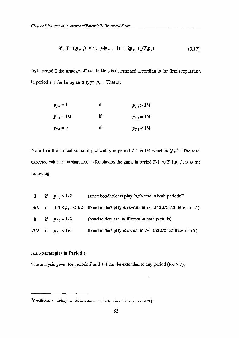
Chapter 3 Investment Incentives of Financially Distressed Firms
WB(TlpT_l) = YT_1(4Pr_1 i) + 2PT_l1'b(TJT) (3.17)
As in period T the strategy of bondholders is determined according to the firm's reputation
in period T-1 for being an a type, Pr-i- That is,
Yr-i=1 if PT-i>114
Yr-i = 1/2 if Pr-i = 1/4
YT-i=° if
Note that the critical value of probability in period T-1 is 1/4 which is () 2. The total
expected value to the shareholders for playing the game in period T- 1, v3(T- "PT-i), is as the
following
3 if Pr-i > 1/2 (since bondholders play high-rate in both periods)9
3/2 if 114 <Pr-i < 1/2 (bondholders play high-rate in T-1 and are indifferent in 7)
0 if Pr-i = 1/2 (bondholders are indifferent in both periods)
3/2 if Pr-i < 1/4 (bondholders play low-rate in T-1 and are indifferent in 7)
3.2.3 Strategies in Period t
The analysis given for periods T and T-1 can be extended to any period (for t<zT).
9Conditionai on taking low-risk investment option by shareholders in period T-1.
63

p (1 —PT)0
(1 _pt)pT(T_o)(3.18)
Chapter 3 Investment Incentives of Financially Distressed Finns
Strategies of Bondholders
Bondholders consider the reputation of the firm for being an a type, p,, when rating the
firm's bonds in period t. Thus, ifp jiT)Tl , they give high-rating (i.e. y=l). If, however,
Pt<(PT), they give low-rating (i.e. y 1=O). And jf pt=(p T) T-t+l , they randomize giving high-
rating with probability 1/2.
Strategies of Shareholders
If the firm is an a type, shareholders always choose the value-maximising decision, i.e, they
take the low-risk investment. If the firm is a 3 type, the decision of shareholders depends
P . If P>(.Pr)Tt, shareholders choose the low-risk investment option with certainty. If
O<p1<(j5)Tt, shareholders choose the high-risk investment option with a positive probability.
In other words, they take the low risk-investment with probability
and chooses the high-risk investment with the complementary probability.'0
The above argument can be explained by the following figure.
10 It should be noted that if p,=O, the probability of choosing the low-risk investment is zero, and theprobability of choosing the low-risk investment is one.
64

1/2
p0
0
Chapter 3 Investment Incentives of Financially Distressed Firms
T-t+ I'2)
k T t
Figure 3.2 Reputation Acquisition
Figure 3.2 plots the reputation of shareholders against time. Supposing that the initial
probability that the firm is of an a type is p0, there is a sequential equilibrium in this game
where bondholders give high-rating to the firm and the firm chooses the low-risk investment
option until period k. Afterwards there is always a chance that the bondholders will give
low-rating to the firm since in period k bondholders are for the first time indifferent between
low-rate and high-rate. Also, there is non-zero probability that the shareholders will choose
the high-risk investment option. As noted earlier, the probability of playing low-risk must
be less than one in order to be able to enhance the reputation when the reputation in the
current period is less than the critical value of the next period. In other words, during the
reputation building phase, beliefs about the type of the firm are only updated when the firm
chooses the low-risk investment option while there is a non-zero probability that it will
choose the high-risk investment option. Thus, if shareholders choose the low-risk
investment the reputation of the firm advances up the locus shown and the game is repeated.
65

Chapter 3 Investment Incentives of Financially Distressed Firms
3.3 Conclusions
This chapter has analysed the distortion in the investment incentives of financially distressed
firms. The analysis demonstrates that when there is asymmetric information between
shareholders and bondholders about the true financial condition of the firm shareholders
may tend to deviate from value maximising decisions if the firm is in financial distress. They
may have incentives to invest in negative NPV projects (risk shifting problem) and pass up
valuable (but unobservable) investment opportunities (underinvestment problem). This
reduces the value which bondholders expect to get upon liquidation, where shareholders
do not receive any payment since the total liquidation value of the firm's assets does not
meet its total obligations. The problem of risk shifting is curtailed to some extent when
bondholders give ratings to the firm's bonds according to its reputation for being a value-
maximising firm. This is the positive reputation effect in the sense that shareholders'
attempt to gain reputation leads to a reduction in their incentives to invest in risky projects.
However, shareholders of a fmancially distressed firm do still pass up some other
investments which are not observable by bondholders. By having a high enough reputation,
which leads bondholders to give high rating to the firm's bondholders, shareholders can have
a higher level of non-pecuniary benefits by spending the proceeds of foregone unobservable
investments. This can be called negative reputation effect. This is because the firm in
financially distress wifi continue to pass up valuable investment opportunities after the bond
finance is secured as a result of the firm's reputation.
One important implication of this analysis is that fmancially distressed firms might
follow a different investment strategy from other firms which face the same investment
opportunities. They might attempt to delay bankruptcy in order to get benefits from non-
66

Chapter 3 Investment Incentives of Financially Distressed Firms
pecuniary expenditures. In order to be able to do this shareholders try to increase their
reputation for being a value maximising firm by taking those investments which are observed
by the market. As long as they get high rating in the bond market they pass up unobservable
investments. In behaving in such a way shareholders transfer wealth from bondholders.
This may be regarded as one type of costs of financial leverage.
Another implication is that asset type distinction plays an important role in generating
these costs. The games played at the expense of bondholders are more likely to exist when
potential ex post liquidation costs are high. Given the fact that intangible assets lose a
substantial amount of their values when they pass through the bankruptcy procedures firms
having more intangible assets and facing an imminent bankruptcy are more likely to deviate
from value maximizing decision. Shareholders may not take valuable investments since this
means a wealth transfer to bondholders. As a result, bondholders may be reluctant to buy
bonds of a firm which is highly levered and has assets which do not have many other
alternative uses.
67

CHAPTER 4
CORPORATE BANKRUPTIES AND THE ROLE OF BANKS

Chapter 4 Corporate Bankruptcies and the Role of Banks
4.1 Introduction
In the previous chapter a reputation model was developed, where shareholders of firms in
financial distress have incentives to establish a reputation for being value-maximizer who
behave in the interest of all claimholders of the firm. That is, the model in chapter 3
emphasized the role of reputation acquisition on the debtor's side. The present chapter, on
the other hand, attempts to explore the role of reputation on the creditor's side and analyses
the implications of reputation acquisition by banks for financially distressed firms.
The role of banks in providing finance to firms has been of considerable interest in
finance. It has been argued that banks are better informed than other lenders in producing
information about borrowers (Leland and Pyle (1977), Diamond (1984), Sharpe (1990),
Rajan (1992)). Another argument is that banks are better suited to renegotiate loans and
have greater ability to restructure debt contracts. This flexibility of banks is unavailable in
the capital market due to coordination problems among multiple public debtholders (Gertner
and Scharfstein (1991), and Thakor and Wilson (1995)). Several recent studies have also
studied the choice between bank loans and publicly traded loans by using reputation
acquisition models. For example, Diamond (1991) analyses the choice between borrowing
through banks and borrowing directly by issuing publicly traded bonds or commercial paper.
The model shows that borrowers establish reputation by repaying loans from a bank that
monitors to alleviate moral hazard in the initial periods and then issue debt directly without
monitoring by using their good track record from the monitored borrowing. Chemmanur
and Fulghieri (1994a) also develops a reputation model where the focus is on reputation
acquisition by banks. They argue that banks' treatment of financially distressed firms might
be fundamentally different from that of holders of publicly traded debt (bondholders) since
69

Chapter 4 Corporate Bankruptcies and the Role of Banks
banks have incentives to develop a reputation for being more flexible to borrowing firms in
fmancial distress since they are long-term players in the debt market.' It is shown that, in
equilibrium, firms with a relatively high probability of being in financial distress prefer bank
loans to publicly traded debt, even though the interest rate on bank loan is higher.2
However, the behaviour of banks towards fmancially distressed firms sometimes
becomes a focus of criticism (see Keasey and Watson (1994) for a review of the UK case).
From a theoretical perspective, a lender's response to a firm in financial distress is viewed
by the banking literature as consisting of two alternatives: liquidation or restructuring the
debt (continuation) (e.g., Bulow and Showen (1978), Gertner and Scharfstein (1991)).
Banks are criticised for forcing firms into liquidation especially when they have higher
continuation values than liquidation values of their assets. Nevertheless, there has been no
satisfactory explanation as to how banks benefit from such behaviour. One explanation
given by Keasey and Watson (1994) is that banks, being aware of the incentives of
financially distressed firms to act in a manner which results in a shift in the distribution of
business risk onto the bank, may view liquidation as the preferred course of action even if
this decision is seen by firms as an economically irrational decision. Another explanation is
due to Asquith et al (1994). They argue that when there are many public creditors, each
creditor has an incentive to free ride and not loosen financial constraints on firms by, for
example, deferring principle and interest payments and providing new financing. This
behaviour, in turn, discourages banks to make concessions because public creditors are
tThe flexibility of banks towards borrowing firms has been also pointed out by other authors (see, e.g. Gilson,John and Lang (1990), and Hoshi, Kashyap and Scharfstein (1990 and 1991)).
2Other studies which use reputation acquisition model in finance include John and Nachman (1985), Webb(1987), Diamond (1989), Maksimovic and Titman (1991), Chemmanur and Fuighieri (1994b).
70

Chapter 4 Corporate Bankruptcies and the Role of Banks
likely to receive some of the gains from a restructuring between the bank and the firm
whereas the bank bears the full cost of such restructuring. Frankel and Montgomery (1991)
point out another aspect of the problem. They argue that the form of relationship in banking
system between a bank and its customers can influence the resolution of the fmancial
distress. Bankruptcy rules in the UK and the US are compared with those in Germany and
Japan to argue that bankruptcy laws in the former two countries discourage banks to form
a close relationship with firms in financial distress whereas banks in Germany and Japan are
encouraged to participate in informal corporate rescues. Their argument suggests that there
will be fewer rescue attempts and more liquidations in those countries where the relationship
between banks and firms is not close.
Our objective in this chapter is to provide more insight into the incentives of banks
towards fmancially distressed firms. In doing this, reputation of banks is brought into the
analysis. it is argued that banks might have different incentives than those discussed in the
existing literature. More specifically, when banks face financially distressed firms
sequentially they might have an opportunity and a desire to establish a reputation for being
tough against firms in financial distress. They may attempt to develop this reputation by
liquidating even those firms that experience temporary financial difficulties and have greater
continuation value than their liquidation values. In our model, reputation acquisition
provides incentives even for banks which have no immediate advantage from liquidating
firms in financial distress. However, the short-term loss from liquidating firms might be
weighed by the long-term gain by preventing future defaults. Bankruptcy decisions of banks
which face a fmancially distressed firm which cannot honour its debt obligations are
determined by a trade-off between acquiring reputation for being tough by liquidating the
71

Chapter 4 Corporate Bankruptcies and the Role of Banks
firm (but losing some part of the debt and interest repayments in terms of liquidation costs)
and restructuring the debt so as to increase the proportion of repayment (but weakening the
position against future defaults). In the model, reputation acts as a commitment device
which enables banks to credibly threaten borrowing firms to force them into liquidation in
the event that they default on their debt obligations.
Reputational considerations in this context might partly explain why some firms are
inefficiently liquidated by banks even when their going-concern values are greater than
liquidation values of their assets. To put it differently, some of the company bankruptcies
may be caused by the behaviour of the 'reputable" banks which liquidate financially
distressed firms in response to anticipated higher payoffs when facing other troubled firms.
This analysis might also offer an explanation for the relatively high number of voluntary
liquidations which are less costly compared to compulsory liquidations. Moreover, the
model implies that small-medium firms are more likely to be liquidated when they are in
financial distress since the costs they impose on banks upon liquidation are negligible
compared to the costs imposed by large firms. Costs of financial distress play an important
role when discussing the reputation effects. In particular, it is shown that banks may choose
to accept to reduce the current obligations of a financially distressed firm when the costs of
liquidating the firm are very high, and wish to let the firm be liquidated and acquire
reputation for toughness against financially troubled firms when such costs are low.
The rest of the chapter proceeds as follows. In the next section the reputation model
is developed, where one bank faces two financially distressed firms sequentially. In section
4.3 the model is extended to include N firms. Finally conclusions are listed in section 4.4.
72

Chapter 4 Corporate Bankruptcies and the Role of Banks
4.2 The Model
The basic model comprises an agency relationship between two groups of players: two firms
(firm 1 and firm 2) and a bank. In this two date (time 1 and time 2) model, firm i which is
financially distressed takes decision either to default on principal and interest payments,
(D 1+rD1), or to liquidate voluntarily (where i=l,2). Following the firm's decision, if it is
default, the bank has to choose either to accept to reduce the interest and principal payments
or to reject and liquidate it by pursuing legal actions. 3 If, however, firms do not default on
their debt obligations the bank does not have to take any action. The game which will be
described below starts at time 1 and is repeated at time 2. That is, the bank plays the game
against each firm in turn: First, it confronts firm 1, then firm 2. Each firm is assumed to be
experiencing temporary financial difficulties. Although they can not meet the current
obligations the going-concern value of firm i, 6., is greater than its current obligations
(D 1+rD1). In other words, firms are insolvent only on aflow-basis, not on a stock basis.4
Firms differ in terms of the costs of financial distress they incur and impose on the bank,
which are assumed to be limited to the costs of liquidation 5 , and the total obligations.
There are three possible ways of resolving the financial distress. Firstly, the insolvent
firm can voluntarily liquidate itself. This is the least costly way since it does not require
court involvement and the firm's assets can be sold at a higher price because of a higher
3it is assumed that all legal actions against the financially distressed firm lead to liquidation of the firm.
4Although they might have different meanings in some other contexts both "insolvent firm' and "financiallydistressed firm" will be used interchangeably throughout this chapter to mean the same thing.
5As discussed in other chapters the liquidation values of insolvent firms might change substantially across firmsdepending upon the nature of assets they hold. Some assets (e.g. tangible assets) might fetch higher value thanothers (e.g. intangible assets) when liquidated. (For an extensive treatment of this issue see, e.g., Alderson andBetker (1995) and Shleifer and Vishny (1992)).
73

Chapter 4 Corporate Bankruptcies and the Role of Banks
chance of being sold as a going concern under the incumbent management. Nevertheless,
financial distress is not costless and shareholders of the firm still lose an amount of e ,O, and
hence receive (l-cOr(Dj+rDj) upon voluntary liquidation, where e represents the ratio of
the costs of liquidation to the value of firm i. Secondly, the bank might not pursue legal
actions against the insolvent firm and accept to reduce its current obligations. In this case,
the shareholders are entitled to have the going-concern value, O, and their payoff will be
Or(18 1)(D,+rDj) where 81 is the reduction on the total current obligations of firm i.
Thirdly, the firm's assets can be sold through a compulsory liquidation. Under this
procedure, it is assumed that, there will be no value left for shareholders of the firm and,
because of the limited liability, their payoff will be 0.
The bank might be of two possible types, "strong" or "weak". A strozig-type baek.és
assumed to incur less costs than a weak-type bank when it liquidates financially distressed
firms. This might be because, for example, strong-type banks might have more experts than
weak-type banks to deal with insolvent firms more efficiently. It is also possible that costs
of liquidating firms in financial distress may not be limited to direct costs of liquidation but
there might also be indirect costs such as side effects on other customers, losing new
customers and so on. It can be argued that these costs might be higher for some banks
(weak banks) than others (strong banks). The payoffs of strong and weak type banks are
given by (1-a1)(D,-i-rD,) and (l-?b)(D1+rD1) respectively when they choose to liquidate the
insolvent firm i, where a 1 and ), represent the proportional costs of liquidation which strong
and weak-type banks have to incur when they liquidate firm i. The payoffs of the two types
are the same when there is no default or the current obligations of firms are reduced, given
by (D,+rD,) and (1-81)(D1-i-rD,) respectively, where ô.(D1-1-rD,) gives the amount of the
74

Chapter 4 Corporate Bankruptcies and the Role of Banks
reduction in the principal and interest payments of firm i.
It is assumed that (l-ô1)(D,+rD) is less than (1-a1)(D,+rD1) so that it is profitable
for the strong-type bank to liquidate the insolvent firm whenever it defaults on its current
obligations. However, it is more costly for the weak-type to liquidate the insolvent firm than
to reduce its obligations so that (l-8 1)(D 1+rD 1) is greater than (l-?.1)(D+rD,). As will be
discussed later in this chapter the value of ô, is determined by firm i. It is important to note
that the reduction ratio ô 1 cannot be less than ô7 where (1o,* ) is the maximum proportion
of the firm's current obligations which it can meet. It is assumed that even if ô 1=ô 1 " the
payoffs are such that (1 -2. 1)(D,+rD1)<( 1- ô 1*)(D1+ rD 1)<( 1-a,) (D1 +rD 1). The corresponding
payoffs to the insolvent firm and the bank which can be of two types, depending upon the
actions they choose, are given in Table 4.1 •6
Table 4.1 Payoffs to an Insolvent Firm and a Bank Which Can be of Two Types
Decisions Insolvent Firm, Strong Bank Weak Bank
Voluntary Liquidation (1-E,)O,-(D,+rD,) D.+rD, D,-i-rD,
Accept O,-(1- 8 ,)(D,+rD1) (1-8 ,)(D,+rD 1) (1-8 ,)(D14-rD,)Default
Reject 0 (1-a,)(D,+rD,) (1-?j(D,-i-rD,)
Notes: a <8,<? where i=l,2.
61t may be argued that debt obligations of financially distressed firms can be rescheduled by banks given thatfirms are solvent on a stock basis. This option can be incorporated into the model by replacing voluntaryliquidation option by debt rescheduling and setting s ,=0. This would not change the implications of the modelsubstantially and the model could be reinterpreted accordingly. In this case it is still possible that firms can crediblythreaten banks to default as long as (1-8 ,)(D,+rD,) exceeds (l-A,)(D,+rD,) and there is a sufficient probability ofthe bank being of weak-type.
75

Chapter 4 Corporate Bankruptcies and the Role of Banks
In the model, firms cannot identify which type of the bank they deal with. That is, there is
informational asymmetry between the bank and firms about the characteristics of the bank.
The bank knows its own type, whereas firms observe only a priori distribution over the
bank's type. It is common knowledge that the strong-type bank always liquidates firms
which default on their obligations. Thus, by assessing the probability of the bank being of
strong-type firms attach a credibility to the bank's actions. In this sense, this probability can
be interpreted as the reputation of the bank. At time 1 firms have a prior probability of Pi'
p1 (0,1), of the bank being a strong-type, and (l-pi) of the bank being a weak-type. At
time 2, they update this probability to P2 depending upon whether additional information is
revealed about the bank's type at time 1. If there is no default at time 1, in which case the
bank is not called upon to take an action, no additional information is observed by firm 2.
The equilibrium concept used in this model is based on the "sequential equilibrium"
of Kreps and Wilson (1982). In the context of this finite horizon game analysed in this
chapter, an equilibrium consists of a behaviour strategy by each player that satisfies the
following conditions: (i) The choices made by the bank are best response to the firm's
choices at each date, given the set of equilibrium beliefs formed by the firms in response to
these choices; (ii) The beliefs of the firms are consistent with the bank's strategy, given the
history of prior play and that the bank is a strong-type with probability p which is computed
using Bayes' rule. Bayes' rule requires that
Prob(llquidates I strong) Prob(strong)2 Prob(liquidates I strong) Prob(strong) + Prob(liquidates I weak) Prob(weak)
and, since the strong-type bank always liquidates it reduces to
76

Chapter 4 Corporate Bankruptcies and the Role of Banks
p1p2 =
(4.1)p1+31(1—p1)
where [) is the probability that weak-type bank liquidates firm 1 at time 1 and P2 is the
updated probability assessment that the bank is of strong-type. One interpretation of Bayes'
rule might be that learning takes place in the form of using observation in order to form a
better probability estimate of the type of the bank. In other words, by means of evidence,
prior beliefs are converted into posterior beliefs. In the context of our model, a prior
probability of Pi at time 1 that the bank is a strong-type is converted to a posterior
probability of p2 after observing that the bank liquidates the insolvent firm at time 1.
The notion behind the game below is that a bank when facing firms in financial distress
repeatedly may have incentives to develop a reputation for being tough against these firms.
The idea is that if the bank always plays in the same way (liquidates when firms default on
their debt), other financially distressed firms will expect the bank to continue to play in the
same way in the future and wifi adjust their own strategy accordingly. The question is then
whether and under which conditions it is desirable and possible for the bank to develop the
reputation it desires. The rest of this section attempts to answer this question.
We can now outline the game starting by explaining how P2 is computed. If firm 1
does not default at time 1, no additional information is revealed about the type of the bank
and hence P2 is set to be equal to the initial assessment (reputation) given by p . If either
Pi=° or firm 1 defaults and is not liquidated by the bank, this reveals the type of the bank
as weak and hence p2=O. if, however, default is met by legal action and p 1 >O, then the initial
77

Chapter 4 Corporate Bankruptcies and the Role of Banks
probability that the bank is a strong-type is updated by Bayes' rule. Since, given that the
bank liquidates firm 1 at time 1, the main motivation of the bank is to deter firm 2 from
defaulting one should start by analysing how firm 2's decision is determined at time 2.
4.2.1 Strategy of Firm 2
If firm 2 decides to default it nets from defaulting
p2(0) + (1-p2) [02 -(l -ô 2)(D2 +rD2)] (4.2)
where P2 is the probability at time 2 that the bank is of strong-type. If it defaults and the
bank is of strong-type the payoff of firm 2 is zero and 02-(1-ô 2)(D2+rD2) if the bank is of
weak-type. P2 plays a crucial role in decision making of firm 2 since it is common
knowledge that, at time 2 which is the last period, the strong-type bank certainly liquidates
the insolvent firm whereas the weak-type bank does not since it is more costly to do so and
there are no further periods to enjoy the reputation for being of strong-type. Firm 2 defaults
if its expected payoff from defaulting, given by (4.2), exceeds its payoff from liquidating
itself voluntarily. That is, it defaults if the following inequality holds
(1 -p2)[O2 -(1 -8 2)(D2 +rD2)J > (1 2)°2 -(D2 +rD2) (4.3)
From the above inequality one can derive a critical value of p 2 , below which firm 2 decides
to default, which is given as
- - c 202 + ô2(D2-i-rD2)
P2 - 02-(1-ô2)(D2+rD2)(4.4)
78

Chapter 4 Corporate Bankruptcies and the Role of Banks
Thus, financially distressed firm 2 decides to default if
c 202 + ô2(D2-i-rD2)
< 02-(1-82)(D2+rD2)
and does not default if the inequality is reversed. 7 If P2 =15 2 the firm 2 randomizes , i.e. it is
indifferent between defaulting and liquidating itself voluntarily. In this case the expected
payoffs from defaulting and voluntary liquidation are the same. This can be explained
referring to Figure 4.1 where the horizontal axis gives the probability of the bank being of
strong-type, p2 , and the vertical axis the difference between the expected payoff to firm 2
under default, (1-p2){02-(1-ô 2)(D 2+rD 2)], and its payoff under voluntary liquidation, (1-
e 2)02-(D2+rD2). As P2 increases the expected gain from defaulting decreases and becomes
zero when P2=P2 As long as the reputation of the bank for being of strong-type, given by
P2' is less than 152 the expected payoff from defaulting exceeds that from voluntary
liquidation and hence firm 2 defaults. When P?'P2 firm 2 does not default since its expected
payoff from doing so is less than its payoff under voluntary liquidation. If, in the extreme
case, P2=1 then the difference between the two payoffs reaches its maximum and becomes
-(1-c 2)02+(D2+rD2) which shows that by defaulting against the strong bank the insolvent
firm loses the amount it would have received under voluntary liquidation.
7 So far it has been assumed that the firms payoff from voluntary liquidation is positive, i.e. (1-c 2)0 2-(D2+rD2)>O. However, it might be the case that the pmceeds of the voluntary liquidation, (l-e 2)0 2, might fall belowthe firms total obligations, (D2+rD2). This might happen, for example, when the liquidation costs, 6 20 2 , or the totalobligations of the firm are large enough so that the firm gets nothing upon a voluntary liquidation. Then, theinequality (4.3) always holds since the left hand side is positive as long as P2 is not one. This is because [0 2-(l-o 2)(D2-i-rD2)] is always greater than zero (it would not be rational for the firm to ask a reduction which would notlead to a positive payoff). Thus, in this case firm 2 would default even if p2 is very big. However, in the rest ofthe chapter we continue to assume that the payoffs to the insolvent firms from liquidating themselves voluntarilyare positive.
(4.5)
79

c 202 +ô2(i
-(1-82)02+
Chapter 4 Corporate Bankruptcies and the Role of Banks
Figure 4.1 Expected Gain from Defaulting
It might be useful at this point to discuss the determinants of the critical probability, p2 . The
value of J2 changes with changes in the ratio of the costs of voluntary liquidation, c 2' the
going-concern value of the firm, 02, and the total of principal and interest payments,
(D2 +rD2). For example, p2 increases if 8 2 rises, ceteris paribus. This is because the
difference between what firm 2 gets under restructuring and what it receives under voluntary
liquidation, given by the numerator in (4.4), gets larger. 8 This implies that, given the
reputation of the bank being of strong-type, the probability that firm 2 will default increases.
This can be seen in Figure 4.1 as p2 moves to the right towards 1. It is also clear from
Figure 4.1 that the point at which the difference line intersects the vertical axis shifts
upwards as 8 2 increases. Similarly, an increase in (D2+rD2) or a decrease in 02 leads to an
increase in the critical probability. In the former case, the numerator increases whereas the
8Note that the increase in the difference is due to the decrease in the payoff under voluntary liquidation. Thepayoff under restructuring, given by the denominator, remains the same.
80

Chapter 4 Corporate Bankruptcies and the Role of Banks
denominator decreases. This in turn implies that the higher the insolvent firm's debt is the
higher the probability is that it will default on its debt in financial distress. In the latter case,
a decrease in 02 decreases both the numerator and the denominator. However, the change
in the value of the numerator is less than that of the denominator so that the overall
probability increases. The interpretation of this result might be that fmancially distressed
firms might be more willing to take the risk of being liquidated compulsorily as the
continuation value of their assets decreases, ceteris paribus. To summarise, default is more
likely for those financially distressed firms which have to incur relatively high costs under
voluntary liquidation, have low going-concern value and/or large amount of debt.
It is discussed above that one of the determinants of 2 is the costs of voluntary
liquidation and argued that the probability of firm 2 defaulting rises when c 2 increases. This
is also true for the costs of compulsory liquidation. As will be explained later in this chapter
the value of 8 2 is directly related to the ratio of the costs of compulsory liquidation, 2
That is, if the costs of compulsory liquidation increases then the reduction asked by firm 2
also increases, which in turn raises . One important implication of this result is that firms
with those assets whose values substantially decrease in liquidation (voluntary or
compulsory) are more likely to default when they are in financial distress.
4.2.2 Strategy of the Bank
As mentioned earlier, the strong-type bank always liquidates the insolvent firm which
defaults because the return from liquidating the insolvent firm, (1-a )(D 1+rD 1), is always
greater than the return from accepting to reduce its debt obligations, (l-8 1)(D1+rD1). If the
bank is weak, however, there are several cases to consider when the financially distressed
81

Chapter 4 Corporate Bankruptcies and the Role of Banks
firm decides to default. The weak bank's response depends on the date, t, and p,.
(i) if t=2, the weak-type bank does not liquidate the firm which defaults, since the
liquidation is more costly, and there are no reputation effects to consider beyond time 2.
The weak-type bank always finds it advantageous to reduce the insolvent firm's debt at time
2. It maximizes its payoff in the last period by accepting to reduce the firm's obligations.
The weak-type bank liquidates the insolvent firm only if the payoff from liquidation exceeds
what it gets when it accepts to reduce the obligations of firm 2 which can be stated as
(1-?..2)(D2+rD2) > (1-8 2)(D2 +rD2)
(4.6)
This condition does not hold since . 2>ô 2. That is why the weak-type bank never liquidates
the insolvent firm in the last period. The value to the bank at time 2, vb(t=2 ,p2), depends
on the probability that the bank is of strong-type, p2 . It is given as
(D2-I-rD2)
if P>P
(firm 2 voluntarily liquidates)
(1- ô 2)(D2-i-rD2)
if P2<P2 (firm 2 defaults)
(1- ô 2"2) (D2-i-rD2)
if P2=P2 (firm 2 is indifferent)9
(ii) if t= 1, the bank must consider the impact of its current action at time 2. Since the
bank's return is higher at time 2 if firm 2 believes that it is of strong-type, the weak-type
bank has an incentive to act as though it is a strong-type and to liquidate firm 1 at time 1.
91t should be noted that when p2=p2 firm 2 is indifferent and defaults with probability 1/2 and hence the value
to the weak bank becomes 1/2(D2 +rD2)+1/2(1-8 2)(D2 -1-rD2) which gives (1-8 2/2) (D2-frD2).
82

Chapter 4 Corporate Bankruptcies and the Role of Banks
The total expected return to the bank, when firm 1 defaults, takes the form of
Eb(t=1 p l)) = + (1-31)[(1-ô1)(D1+rD1)]
+ 13 1vb(t=2,p2) + (1-131)[(1-ô2)(D2-i-rD2)] (4.7)
The last term in (4.7) shows that if the bank fails to liquidate firm 1 at time 1, which occurs
with the probability (1- 1 ), then the bank's type is revealed as weak and hence the reputation
for being strong is lost. It follows that firm 2 chooses to default at time 2 expecting that the
bank will reduce its obligations and the bank accepts to reduce. Thus, the payoff to the
bank in the last period becomes (1-ô 2)(D2 +rD2). The penultimate term, on the other hand,
reflects the probability of liquidating the insolvent firm at time 1 and corresponding payoff
at time 2 associated with a reputation P2 Equation (4.7) can be rearranged as the following
Eb (t=lp l) = 1 [vb(t =2p2) ^(D 1 -i-rD 1)(ô 1 -(1 -ô2)(D2-i-rD2)]
+ (1-ô 1)(D 1 -i-rD 1) + (1-ô2)(D2+rD2) (4.8)
As explained earlier the bank is entitled to get vb(t=2 ,p2) at time 2 when it liquidates the
insolvent firm at time 1. Since the value of vb(t=2,p2) depends on P2 the bank is concerned
about how its decision at time 1 affects its reputation at time 2, which is given by P2• Three
different cases might arise depending upon the value of the initial probability of the bank
being of strong-type, p 1 . and its relation to the critical value of the probability, above
which the insolvent firm at time 2 chooses to liquidate itself voluntarily.
(a) If p > P2 the posterior probability of the weak-type bank being of strong-type,
83

Chapter 4 Corporate Bankruptcies and the Role of Banks
given that it liquidates firm 1, will be at least Pi (i.e., p2=max(p 1 ,j52)) since the strong-type
bank always liquidates. Liquidating firm 1 prevents firm 2 from defaulting because it is
known from the above analysis that firm 2 does not default when P2>172 (note that P2=P1>
P2) . Although the reputation of the bank does not change it is sufficient to ensure that firm
2 expects to be liquidated when it defaults. The behaviour of the weak-type bank may be
explained as follows. Since Pi' the initial probability that the bank is of strong type, is high
enough the insolvent firm at time 2 will believe that it faces a strong-type bank if the bank
has liquidated the insolvent firm at time 1. This gives the weak-type bank a strong incentive
to maintain its reputation at time 1 when it decides whether to liquidate firm 1. However,
although it ensures that firm 2 wifi not default given that the bank liquidates firm 1, p is not
alone sufficient to explain the strategy of the bank at time 1. Whether the bank liquidates
the insolvent firm 1 at time 1 also depends on the value inside the square bracket. It must
be greater than or equal to zero for f3 being equal to one since is chosen to maximise
(4.8). That is, the following inequality must hold
Vb(t =2p2) +(D 1 +rD 1)(ô 1 -A 1) -(1 -ô 2)(D2 +rJJ2) ^ 0 (4.9)
It is known that vb(t2,p2) is (D2 +rD2) when P2>17. Then, (4.9) can be rearranged as
ô 2(D2 +rD2) ^ (D 1 +rD1)(A 1 -8 1) (4.10)
The interpretation of this result is useful.'° Here, ô 2(D2+rD2) can be interpreted as the
101'he condition given in (4.10) can alternatively be derived by considering the returns of the bank. Thebank's total return is (1-A 1)(D 1 +rD 1)+(D2+rD2) if it liquidates firm 1 when PI>P2 (since firm 2 voluntarily liquidatesat time 2). On the other hand, the weak-type bank receives (1-o 1 )(D 1 +rD 1 )+(1 -o 2)(D2+rD2) if it does not liquidate
84

Chapter 4 Corporate Bankruptcies and the Role of Banks
amount of the loss which the weak-type bank has to incur at time 2 if it fails to liquidate firm
1. This is because firm 2, knowing that the bank is of weak-type and hence does not choose
to liquidate the insolvent finn in the last term, certainly defaults on its debt obligations."
(D,+rD,)O,-ô,), on the other hand, can be seen as the bank's loss at time 1 from liquidating
firm 1. The trade-off which the weak-type bank faces should be now clear. The bank
chooses to liquidate the insolvent firm at time 1 in order to keep its reputation towards firm
2 only if the cost of doing so is less than or equal to the cost of not doing. It should be clear
from (4.10) that for (D,+rD,) and/or ?., big enough the bank's loss from liquidating firm 1
exceeds the loss it incurs when it does not liquidate firm 1. In this case the liquidation costs
which the weak-type bank has to incur by liquidating firm 1 are more important than its
reputation which will prevent firm 2 from defaulting. Therefore, the bank decides not to
liquidate firm 1 even though p,)' 2 . This can be clarified further by rearranging (4.10) as
the following
D-i-rD
D+rD (4.11)
Now, the LHS of the inequality (4.11) is the ratio of the proportional loss incurred at time
2 (if not liquidate firm 1) to the proportional loss incurred at time 1 (if liquidate firm 1). The
RHS of (4.11), on the other hand, gives the ratio of total current obligations of firm 1 to
firm 2's. It is clear that even if the proportional loss at time 2 is higher than the proportional
loss at time 1 the weak-type bank might stifi not want to liquidate firm 1. This occurs when
firm 1. Therefore, the bank decides to liquidate firm 1 at time I only if (l-X,)(D 1 +rD 1 )+(D2-i-rD2) ^ (1-ö 1 )(D 1 +rD 1 )+(l-ô 2)(D2+rD2) which also yields (4.10).
11 8 2(D2+rD2) can also be interpreted as the gain of the bank from liquidating firm 1 given that firm 2 does notdefault and liquidates itself voluntarily.
85

Chapter 4 Corporate Bankruptcies and the Role of Banks
the total obligation of firm 1 is relatively higher enough than that of firm 2 so that the
advantage of liquidating firm 1 is offset.'2
(b) If O<p,< 2' it is not an equilibrium strategy for the weak-bank to liquidate the
insolvent firm at time 1 with probability one. This is because, when =1, the posterior
probability that the bank is a strong-type after liquidating would not deter firm 2 from
defaulting.' 3 In this case, the bank would prefer not to liquidate. Also, it is not the case that
if Pt<P2 the weak-type bank wifi always accept to reduce the insolvent firm's debt obligations
(i.e. 3 ,=O). If this were the case, the gain from liquidating firm 1 would be high since it
would make firm 2 believe that the bank is of strong type and the bank would enjoy a higher
return at time 2. Therefore, the equilibrium must involve mixed strategies when O<p 1 < p2.
The weak-type bank must randomize in a way that makes firm 2 indifferent between
defaulting and voluntary liquidation. This requires that the posterior probability that the
bank is strong-type, P2' conditional on liquidating, be exactly the critical level, p2 . the
probabffity that the weak-type bank liquidates firm 1 at time 1, at which the posterior
probability P2 is equal to the critical value p2, can be derived from the following
t2So far it has been assumed that firm I and firm 2 are different in terms of the size of their obligations to thebank. It is also worth considering the case under which they are the same. In this case (4.10) becomes ) ^
(8 1+ 8 2). Now, the size of the firms' debts does not matter. What matters is the proportional liquidation coststogether with the reductions from the obligations of the firms required by firm 1 and firm 2, 6 and 82 respectively.If?. 1 is less than or equal to the total of 8 and 8 2 then the bank gains from liquidating firm I at time 1. If, on theother hand, A 1 exceeds (81+82) it is not the best strategy for the bank to liquidate firm 1 since the costs of doingit is greater than the costs of not doing so.
t3From Bayes' rule, recalling that the strong bank liquidates with probability 1, it can be seen that the posteriorprobability for being a strong-type, p2, would be equal to p 1 which would not deter the insolvent firm fromdefaulting in the last period.
86

Chapter 4 Corporate Bankruptcies and the Role of Banks
P1
p1+131(1-p1)
p 1(1 -p2)p 1 = _______
P2(1 P1)
(4.12)
(4.13)
That is, the weak-type bank liquidates firm 1 with the probability P1( 1-I)2)I P2( l -P1) and
accept to reduce its obligations with the complementary probability.' 4 When the bank
liquidates firm 1, its reputation for being of strong-type rises to p2 at time 2. It is clear from
(4.13) that, since P,< P2' 3, is strictly less than one. This implies that reputation is only
enhanced (P2>P, given that the bank liquidates) if the weak bank liquidates the insolvent firm
with a probability less than one. Nevertheless, it is not certain that liquidating firm 1 will
deter firm 2 from defaulting. Firm 2 either defaults or voluntarily liquidates with probability
1/2 since P2=P2 In other words, P2 is not sufficient to deter firm 2 from defaulting. So,
(4.7) which gives the total expected return to the bank, when firm 1 defaults, becomes
Eb(t =lp l) = (1 -ô 1)(D1 -i-rD 1) +(1 -82)(D2-i-rD2)
+ 1 [(J. --2)(D2 +rD2) +(ô 1 -A 1)(D 1 -i-rD 1) -(1 -6 2)(D2 +rD2)](4.14)
since, when p2 p2, Vb(t-2,p 2) is (1-ô J2)(D2+rD2). Now, for 3, given by (4.13) to be an
equilibrium solution the following must hold
1 'It follows from (4.13) that when p=rO, the probability of liquidating is zero and one when p 1 = p2.
87

Chapter 4 Corporate Bankruptcies and the Role of Banks
(1 +rD2) +(ô 1 -A 1)(D1 +rD1) -(1 -ô 2)(D2 -i-rD2) ^ 0 (4.15)
which in turn gives the following
--(D2 +rD2) ^ (A 1 -o 1)(D1 ^rD1) (4.16)
Once again, the LHS of (4.16) gives the loss which the bank will incur at time 2 if it fails
to liquidate firm 1 at time 1. However, this is now less than ô 2(D2 +rD2) given in (4.10)
because of the uncertainty about whether firm 2 voluntarily liquidates at time 2 when the
bank liquidates firm 1 at time 1. Firm 2 randomizes between defaulting and liquidating
voluntarily with probability 1/2. The RHS of (4.16) is the same as earlier; the loss of the
bank from liquidating firm which is given by (4.13) is not an equilibrium probability
if the inequality (4.16) does not hold. For example, when the loss which the weak-type
bank has to incur at time 2 when it fails to liquidate firm 1, given by 0 2/2(D2-1-rD2), is less
than the loss it has to incur by liquidating firm 1, given by (A 1 -ô 1 )(D 1 +rD 1 ), then 3=0.
(c) Ifp 1=p2 then the bank liquidates firm 1 with probability one, i.e., 31=1. Again, (31
is an equilibrium probability only if the following inequality holds
-(D2 +rD2) ^ (A 1 -0 1)(D1 ^rD1) (4.17)
It is important to note the difference between the conditions given in (4.10) and (4.17). In
(4.10) the gain from liquidating is 8 2(D2+rD2) whereas it is given by ô 2/2(D2+rD2) in (4.17).
88

Chapter 4 Corporate Bankruptcies and the Role of Banks
The latter is less than the former because of the probability that firm 2 might not default
when p2=p2. One should remember that (4.10) is the condition when P1>p2 and (4.17) is the
relevant condition when m=i-'2. Thus, it follows that as the initial probability that the bank
is of strong-type decreases, the loss incurred at time 2 when firm 1 is not liquidated at time
1 when it defaults also diminishes. Alternatively, by defining ô 2(D2 +rD2) as the proportional
gain from liquidating firm 1, it can be said that the gain from liquidating firm 1 at time 1 in
order to get a reputation for being of strong-type diminishes as the initial probability that the
bank is of strong-type decreases.
4.2.3 Strategy of Firm 1
The total probability that firm 1 will be liquidated when it defaults is
p1(l) + (11)[l(lP2)]
(4.18)p2(l -p1)
which reduces to
P1 I J
(4.19)
Then, the expected payoff to the insolvent firm 1 from defaulting at time 1 is given by
+ (1-!! )(01-(1-ô1)(D1+rD1)) (4.20)P2 p2
Firm 1 defaults if its expected payoff from defaulting exceeds what it gets under voluntary
liquidation. That is, firm 1 defaults if the following inequality holds
89

Chapter 4 Corporate Bankruptcies and the Role of Banks
(1 _ !!)(0 -(1 - ô 1)(D1 +rD1)) > (1-c -(D 1 +rD1) (421)P2
which can alternatively be written as follows
c 1 0 1 +8 1(D 1 +rD1) c 0 +ô 2(D2 +rD2) -[_
22< A -(1-ô 1)(D1 -1-rD 1) 02-(1-82)(D2+rD2)
P 1 (4.22)"1
since
- c 202 + ô 2(D +rD2)P2 =
02 (1 -82)(D2+rD2)(4.23)
Firm 1 liquidates voluntarily if the inequality in (4.22) is reversed.' 5 It can be seen from
(4.21) that an increase inp2 leads to an increase in the expected payoff to the insolvent firm
1 from defaulting, given by the LHS of the inequality. This is due to the decrease in the
probability that the firm will not be liquidated when it defaults, which is given by (1 -p1/2).
This implies that the probability of firm 1 defaulting increases as p2 increases. It follows,
then, that any factor which increases (decreases) p2 also increases (decreases) p1 . This is
not a surprising result and can be explained intuitively as follows. If the critical probability
which deters firm 2 from defaulting increases this means that it is now more difficult for the
bank to deter firm 2. Therefore, the bank is less willing to establish the reputation. As can
15 Note that if the two firms are similar in the sense that (D1 +rD1)=(D2 +rD2), 0 i =0 I=2' 2 then theRHS of (4.22) reduces to (p2)2.
90

Chapter 4 Corporate Bankruptcies and the Role of Banks
be seen from (4.22) the analysis carried out earlier for firm 2 is also valid for firm 1. The
critical level of the probability of the bank being of strong-type, below which firm 1 chooses
to default is less than p 2 which is the minimum probability level needed to prevent firm 2
from defaulting. (This is because cO 1+ô,(D1+rD1) is less than O.-(1-ô,)(D1+rD,). This
implies that as the number of firms which the bank meets sequentially increases the level of
probability which defers insolvent firms from defaulting decreases. The important point is
that even for very small initial probability, the reputation effect might work in very early
periods so that more financially distressed firms choose to voluntarily liquidate themselves.
This can be better seen when we extend the analysis to include N firms in section 4.3.
4.2.4 Determination of Debt-reduction Ratio 8,
So far little has been said about how insolvent firms decide on the reduction of their debt
obligations, 8 1. The nature of the decision making about this variable changes between firm
1 and firm 2. It is known that in the last period the strategy of the bank is determined by
only its type. That is, the strong-type liquidates firm 2 whereas the weak-type accepts to
reduce the firm's obligations when it defaults. Therefore, for firm 2 the best strategy is to
choose the highest 8 2 at which (1-8 2)(D2 +rD2) is still greater than (1-.. 2 )(D2 +rD2). That
is, 8 2 is chosen to be marginally less than '2 so that the weak-type bank still prefers not to
liquidate firm 2. This choice maximizes the expected payoff of firm 2. The value of 8 2 does
not affect the decision of strong-type bank since (1- 2 )(D2+rD2) remains to be higher than
(1-6 2)(D2+rD2). However, firm l's choice of ô is not as straightforward as the choice of
8 2 by firm 2. This is because in some cases the value of 6 1 affects the weak-type bank's
decision. For example, as already shown in the analysis above, when p 1 > 2 the best strategy
for the weak-type bank is to liquidate firm 1 with probabffity one when it defaults, given that
91

Chapter 4 Corporate Bankruptcies and the Role of Banks
(4. 10) holds. It is clear that as long as ô 2(D2 +rD2)^ ? 1(D1 +rD1) inequality (4.10) holds
whatever the value of 8 1 is. Since the gain from deterring firm 2 from defaulting is even
higher than the maximum loss which the bank can incur the postulated strategy 13=1 is the
equilibrium strategy. In this case, ô can take any value between 81* and 1, and the firm is
liquidated if it defaults. However, if 8 2(D2 +rD (/J -rrD ) 1 then firm 1 has an
opportunity to choose ô such that it is not the best strategy anymore for the bank to
liquidate with probability one. In fact, the probability becomes zero. In order for this to
happen the following must hold
8 1 (D 1 +rD 1) < A 1 (D1 +rD 1)-82(D2 -'-rD2) (4.24)
i.e. the amount of the reduction asked by firm 1 must be less than the difference between the
costs of compulsory liquidation of firm l's assets and the amount of reduction asked by firm
2.16 Again 8 1 can not be less than 81* and firm 1 chooses the highest value of 8 1 at which
(4.24) still holds. As long as this condition holds the strategy of firm 1 is determined in the
same way as that of firm 2. That is, the only concern for firm 1 is the initial probability of
the bank being of strong-type, p. Firm 1 decides to default if the following inequality holds
t' 1 (0) ^(1 -p1)[01 -(1 -o 1)(D1 ^rD1)] > (1-c -(D1 +rD 1) (4.25)
Note that for the cases O<p 1 <p2 and p1-Pa the inequality in (4.24) takes the form of
8 1 (D1 ^rD 1) < ? 1(D1 +rD1) -ôJ2(D2^rD2)
92

Chapter 4 Corporate Bankruptcies and the Role of Banks
from which p below which firm 1 decides to default can be derived as
- - 1 o1 + ô1(D1+rD1)p1 -
01-(1-81)(D1-i-rD1)(4.26)
which is very similar to 2 given in (4.6).
For larger ? and (D1+rD1) it is more likely that ?. 1 (D 1 +rD 1 ) will be greater than
ô 2(D2+rD2). As shown above, if this holds the reputation acquisition towards firm 2 is not
worth when firm 1 defaults. The implication of this result is that firms imposing relatively
high costs on banks in liquidation and/or having high amount of debt are more powerful in
bargaining with banks in financial distress.
4.3 Generalization of the Basic Model
The analysis so far, for simplicity, has considered decisions of the bank facing only two firms
at time 1 and 2. The analysis can easily be extended to include more firms. In the following
it is assumed that there are N finns and the bank whose type is not known by the firms faces
these financially distressed firms sequentially, i.e. it faces firm N at time T, firm N-i at time
T-1 and so on.
4.3.1 Strategy of Insolvent Firms
Insolvent firms take the reputation of the bank into account when deciding whether to
default on their obligations or to voluntarily liquidate. That is, financially distressed firm i
decides to default at time t if the reputation of the bank for being a strong-type, p, is less
than j5 which is given by
93

Chapter 4 Corporate Bankruptcies and the Role of Banks
c EO, + ôl(Di+rDi)](4.27)II
i=1
where t1,...,T and i=1,...,N. If, on the other hand, p>pt, then the insolvent firm i liquidates
itself voluntarily. And if p=ji the firm randomises between defaulting and liquidating.
4.3.2 Strategy of the Bank
It is known that if the bank is a strong-type it always liquidates the insolvent firm. If,
however, the bank is a weak-type, its decision depends upon its reputation p. If ^<p<
Pt+2 so that the reputation is sufficient to deter the insolvent firm from defaulting at time t+ 1
(i.e. reputation is too high to destroy), then the bank liquidates firm i with certainty (i.e.
3 = 1) where
- T-t cO. + ô1(D-1-rD)1(4.28)p+i =
As discussed earlier for PF1 to be an equilibrium probability one must compare the returns
of the bank under alternative strategies. In deciding whether to liquidate the insolvent firm
i at time t the weak bank needs only to compare the return from accepting to reduce the
insolvent firm's obligations at t,. . .,T to the return from liquidating the insolvent firm i at time
t and accepting to reduce the obligations of firms at t-1-1,...,T.'7 If the latter exceeds or equal
to the former, then the bank liquidates the insolvent firm. That is, for to be one the
following must hold
' 7Note that in later periods when the current reputation p, is less than the critical level of probability of the nextperiod,, the bank liquidates with a positive probability less than one at which the return from liquidating is equalto the return from reducing the insolvent firm's obligations.
94

Chapter 4 Corporate Bankruptcies and the Role of Banks
N
(1 -A)(D +rD.) ^(D^ 1 +rD.^1) + (1 -o)(D +rD) ^s=i-i-2
N
(4.29)(1-o5)(D+rD)
si
which gives
ô1^1(D^1 +rD. 1) ^ -ô 1)(D +rD.) (4.30)
Now, suppose that Pt+k<Pt< P^k^1 The bank again needs to compare the returns under
alternative strategies. In this case, for 3 =1 to be an equilibrium strategy the following must
hold
(1-).)(D1+rD)+ (D -frD )^ I (1-ô5)(D-i-rD5) ^s=i+1 sii-k+1 431
(1-o)(D5^rD5)
which gives
i-i-k
(D5 ^1D ) ^ (4.32)S =i+1
As earlier the LHS of the above inequality can be interpreted as the total gain of the weak
bank from liquidating the insolvent firm i at time t given that the insolvent firms from time
t+l to t+k do not default on their debt obligations and liquidate themselves voluntarily.
They voluntarily liquidate because the reputation of the bank at time t for being a strong
95

Chcpter 4 Corporate Bankruptcies and the Role of Banks
type, p, is sufficient to deter firms from defaulting.
If O<cv< p ^i, the weak bank randomizes in a way that makes the insolvent firm at
time t+ 1 indifferent between defaulting on its debt obligations and liquidating itself
voluntarily. That is, it liquidates the insolvent firm i with the following probability
= _________
(4.33)
Now the following must hold for 13 to be an equilibrium strategy
(1 -A)(D1 -i-rD.) +(D. 1 -i-rD. 1) +-i!(1 - o^1)(D 1 +rD.1)
N N (4.34)
+ (1-o)(D5-i-rD) ^ (1-ô)(D5+rD8)s=i
which in turn gives
ôi+1D_—i .^1 +rD.^1) ^ (A,-ô1)(D+rD1) (4.35)
Finally if p= the weak bank liquidates the insolvent firm i with probability one, i.e. 3 1.
In this case 3 =1 is an equilibrium strategy only if
2.^1 +rD. 1) ^ (A1-ô)(D+rD) (4.36)
96

Chapter 4 Corporate Bankruptcies and the Role of Banks
4.4 Conclusions
This chapter has analysed the incentives of banks which face financially distressed firms by
incorporating the reputation acquisition of banks. The analysis demonstrates that some
banks (the weak-type ones which do not benefit from liquidating financially distressed firms
in the short-run) have an opportunity and desire to establish a reputation for being tough
against firms having financial difficulties. While the strong-type banks always choose to
liquidate insolvent firms since this minimizes their loss, the weak-type banks determine their
action against financially distressed firms by a trade-off between the costs of liquidating
firms and the benefits of reputation acquisition. In response to higher expected payoffs from
other troubled firms the "reputable" banks might liquidate firms inefficiently. That is, some
firms which have continuation values greater than their liquidation values might be
prematurely liquidated. This is one of the important implications of the analysis of this
chapter.
Another implication is that small and medium firms are more likely to be liquidated
when they have financial problems since the liquidation costs they impose on banks are
negligible compared to those imposed by large firms. Thus, one should expect relatively
more rescue attempts for large firms and more compulsory liquidations for small firms. It
is important to note that although some small-medium firms might have very high leverage
ratios, and some large finns low leverage ratios, the important aspect of debt for the present
analysis is the size of debt, not its ratio.
This analysis might also shed some light on the relatively high number of voluntary
liquidations. Firms expecting to be forced into liquidation by banks may choose to liquidate
97

Chapter 4 Corporate Bankruptcies and the Role of Banks
themselves voluntarily since voluntary liquidations are less costly compared to compulsory
liquidations. The analysis of this chapter also suggests that the costs of liquidation are
crucial for the outcome of financial distress. Firms whose assets fetch relatively a low price
under liquidation are more likely to default in financial distress and have more chance of
their debt being restructured. This in turn implies that banks are less willing to lend to firms
having mostly intangible assets (less marketable, firm-specific, growth opportunities, etc.)
and tangible assets can support more debt in capital structure of firms.
The model has also implications for capital structure of firms. While the traditional
theory of capital structure, which is based on the trade-off between the tax advantage of
debt financing and the costs of financial distress, emphasizes the level of debt, the analysis
of this chapter also points to the structure of debt. Although it has not been the main
concern of the present analysis it is implied that the composition of debt (private vs public
debt) can influence firms' default decisions. Since the possibility of renegotiation of bank
loans is greater than that of public loans and there is a chance that banks respond to default
by forgiving some part of the debt instead of imposing costly liquidation firms can
strategically decide to default as a result of value maximising behaviour.
98

CHAPTER 5
ECONOMICS OF INSOLVENCY PROCEDURES ANDINEFFICIENT COMPANY LIQUIDATIONS

Chapter 5 Economics of Insolvency Procedures and Inefficient Company Liquidations
5.1 Introduction
In the last two chapters we analysed the conflicting interests between firms and their
creditors and their implications for financially distressed firms. This chapter, on the other
hand, considers the incentives of the creditors of financially distressed firms and the role of
insolvency procedures in creating these incentives. The procedures applied to business
failures are thought to be at the centre of bankruptcy cost discussion for two reasons.
Firstly, they might involve large direct costs such as fees paid to insolvency practitioners and
expenses made during the formal procedures.' This aspect is important as the efficiency of
any insolvency procedure should require that the procedure is not wasteful in terms of
money and its length, which determines the ultimate costs borne by firms' claimants.
Secondly, the insolvency law may lead to inefficient and premature liquidations of financially
distressed but efficient companies. This might happen, for instance, under the existing UK
procedures which emphasize the rights of creditors by giving them the right to recover their
claims at the expense of other claimants.
This chapter focuses on the second aspect of the problem. More specifically, the main
objective of this chapter is to extend the understanding of the role of insolvency procedures
in the bankruptcy decision of the creditors of a financially distressed firm. In doing this, two
main UK insolvency procedures; receivership and administration, are brought into the
analysis. It is shown that the nature of these two insolvency procedures gives incentives to
1 In recent years, there have been many examples of high insolvency fees in the UK. One of these is the collapseof the Bank of Credit and Commerce International (BCCI). The UK liquidation costs alone amounted to $133million between July 1991 and January 1993. The liquidation of BCCI is an example of international liquidationand requires complex and long procedures. BCCIs liquidators estimated that creditors might have to accept to bepaid only 30-40 per cent of their claims (Financial Times, 15 June 1993). Polly Peck International, the fruit, leisure,and electronics group, is another example where high professional fees have been charged by insolvencypractitioners. To date, the administrators of Polly Peck have taken for themselves and lawyers at least £16 millionin fees since October 1990 when the administrators were appointed (Financial Times, 15 May 1993).
100

Chapter 5 Economics of Insolvency Procedures and Inefficient Company Liquidations
the creditors of a distressed firm to choose receivership, which in most of the cases leads to
the liquidation of the firm, even when the administration is a more efficient option. We also
derive the conditions under which the above mentioned inefficient outcome takes place.
This chapter also stresses the importance of the type of assets owned by firms in the
bankruptcy decision process. Although a number of authors (see, e.g., Titman and Wessels
(1988), Williamson (1988), Shleifer and Vishny (1992) and Alderson and Betker (1995))
have argued the effects of the asset structure of a firm on its financial structure decision, to
the best of our knowledge, no consideration has been given to the relationship between the
asset structure and the bankruptcy decision of creditors. It is argued in this chapter that
firms with a larger proportion of intangibles to total assets are more likely to be liquidated
when they experience financial difficulties. This result largely derives from the view that
under administration the probability of realising a higher value is not significant enough.
The remainder of this chapter proceeds as follows. Section 5.2 briefly discusses the
importance of insolvency procedures in an economy and reviews the existing UK insolvency
practices. Section 5.3 develops a model to show how the UK insolvency procedures might
lead to premature and inefficient liquidations of distressed firms and discusses the
determinants of an inefficient outcome as well as the role of asset structure. Finally, section
5.4 concludes the chapter.
101

Chapter 5 Economics of Insolvency Procedures and Inefficient Company Liquidations
5.2 Role of Bankruptcy Law and Existing UK Procedures
5.2.1 Role of Bankruptcy Law
It is argued that the general purpose served by a bankruptcy law is to help to complete very
incomplete debt contracts by specifying contingencies in the event of insolvency (see, e.g.,
Aghion et al (1992, 1993)). Bankruptcy law determines the reallocation of claims to a
debtor's assets in the event of default. It also specifies whether and how the control of
assets is transferred by defining rights to future income streams. More specifically, a good
insolvency procedure might achieve two main outcomes. First, by defining more precisely
the creditors' property rights, they can lower the cost of writing contracts, which in turn
should smooth the functioning of financial markets and increase the supply of funds relative
to the supply in the absence of bankruptcy law. Second, an ideal insolvency law can
improve the efficiency of resource allocation by limiting the debtor's rights to control the
assets in all states of the world. This happens because it is believed that creditors, upon
default, may force assets to be reallocated to more productive activities, which implies that
firms with higher continuation values should continue and those with higher liquidation
values should liquidate (value-maximising decision). However, it is also argued by Aghion
et al (1992) that bankruptcy laws are far from achieving these goals in the sense that they
either cause premature liquidations of healthy firms (as in Chapter 7 of the US Bankruptcy
Code) or they are biased towards reorganisation under incumbent management (as in
Chapter 11 of the US Bankruptcy Code).2
2At this point it might be useful to compare briefly the UK insolvency procedures and the US bankruptcyprocedures. Two codes are similar in that creditors are paid the proceeds of the liquidation according to theabsolute priority rule under which administrative expenses of the insolvency are paid first, claims for unpaid taxesand wages second, and the unsecured creditors third. Equity gets the residual, if any. Since the secured creditorshave the claim on a particular asset of the company, they are outside the priority ordering. The main differencebetween the two codes is related to the objectives. In the US, the main objective is to maintain the business as agoing concern, and hence the code has been designed to be highly debtor-oriented. If the company files underChapter 11, managers remain in control of the firm and run the business while a reorganization plan is being
102

Chapter 5 Economics of Insolvency Procedures and Inefficient Company Liquidations
5.2.2 The UK Insolvency Procedures
The insolvency procedures in the UK must be supervised or implemented by an insolvency
practitioner with one exception. This is "schemes under section 425 of the Companies Act"
under which a company may institute a rescue plan with its creditors. Creditor agree not
to take any legal action to recover their debts. The advantage of this arrangement is that
once a three-quarters majority in value of the creditors vote in favour of it and the court
sanctions the scheme it binds all creditors and hence the agreement cannot be upset by any
dissenting creditor. However, it is complex and expensive since it involves an application
to court, a calling of meetings of creditors and passing of resolutions. The UK insolvency
procedures fall into four main categories: liquidation, receivership, administration, and
company voluntary arrangement.
5.2.2.1 Liquidation
Liquidation is the process whereby the company's assets are sold and distributed to claim
holders according to their legal entitlements. Liquidators can be appointed by the directors
of the company. This is known as creditors' voluntary liquidation which is the most
commercially effective and hence the most resorted corporate insolvency procedure. There
is no need for an application to court and it is the best alternative if there is little or no
possibility of rescuing the business and selling it as a going concern. If the directors fail to
prepared. Most importantly, all payments of principal and interest on debt cease once in Chapter 11. The directorsof the company can also decide to liquidate the firm by filing under Chapter 7. In the US it is up to the finn'smanagers to decide whether to file for bankruptcy reorganization or liquidation. By contrast, insolvencyproceedings in the UK normally are initiated with a creditor (or a group of creditors) whose claim has not been paid.The main objective of the insolvency code is the repayment of creditors' claims. An insolvency practitionerrepresents the interests of creditors, and in some cases only secured creditors. This makes the UK Code a highlycreditor-oriented code, which encourages premature liquidation (also see Franks and Torous (1992) for acomparison of the efficiency of the UK and US codes and Rajan and Zingales (1995) for the salient features of the
bankruptcy code in the G-7 countries).
103

Chapter 5 Economics of Insolvency Procedures and Inefficient Company Liquidations
pass the necessary resolution for a voluntary liquidation, creditors can liquidate the firm by
obtaining a court order, which is known as compulsory liquidation. It is more expensive
because the court application and supervision are necessary. The liquidator's primary duty
is to recover the company assets for the benefit of the creditors and to distribute funds to
them in accordance with their statutory entitlement. The liquidation procedure terminates
after the liquidator, having paid his fees and the costs of the liquidation, sends his fmal
accounts to the Registrar of Companies.
5.2.2.2 Receivership
Receivers can be appointed either by a floating charge holder, or a fixed charge holder3
when the company defaults in payment of the principal and/or interest due under the loan.
It is also possible to appoint a receiver if the administration petition is presented and the
chargee wishes to appoint a receiver. No court action is necessary for the appointment and
it becomes effective when it is accepted by the qualified insolvency practitioner (receiver).
Since receivership is primarily a recovery procedure for the secured creditor (or group of
secured creditors) the receiver's main responsibility is to protect the interests of the creditor
who appointed him. Therefore, if a rescue plan is not in the interests of such a secured
creditor, the receiver should not pursue it even if unsecured creditors, shareholders and
employees would benefit from this.
3 A floating charge is a charge on the company's property which is constantly changing in nature and notspecifically identified such as its stock in trade. A fixed charge, on the other hand, attaches to a specific item ofcorporate property such as its freehold or buildings. A fixed charge places limitation on the company's dealing withthe assets comprised in it, and hence the firm needs the permission of the debenture holder to deal with the assets,which is not needed under a floating charge. A fixed charge gives the chargee the power to appoint a receiverwhose role is to take possession of and sell the assets and repay the proceeds before the repayment of any othercreditor. Under a floating charge, the chargee can appoint an administrative receiver with an extensive powers ofmanagement such as managing the company's business, borrowing money and hiring staff. Whereas a receiverappointed by a fixed charge holder has no power to continue the business and thus cannot implement a rescue plan,an administrative receiver has adequate powers to achieve a turnaround.
104

Chapter 5 Economics of Insolvency Procedures and Inefficient Company Liquidations
5.2.2.3 Administration
The administration procedure was introduced by the Insolvency Act 1986, which is a formal
court-driven procedure and also available to an unsecured creditor or to the company itself.
The main purpose of administration is to provide a breathing space during which a rescue
plan for the survival of the company can be pursued or the sale of the business as a going
concern can be negotiated. This might provide more advantageous realisation of the
company's assets than would be achieved under liquidation. Administration might be the
preferred option when a company which has a healthy balance sheet and is basically sound
is currently experiencing a cash-flow crisis which makes the company unable to pay its debts
as they fall due (Campbell and Underdown (1991)). Administration is not the end of the
insolvency procedure so far as the company and the creditors are concerned. It is only a
breathing space protected by a legal suspension of payments and may be followed either by
the return of the company in solvent to the control of the company's directors or by the
liquidation of the business.
5.2.2.4 Company Voluntary Arrangements (CVAs)
It is an insolvency procedure under which the management puts up a restructuring proposal
to creditors and continues to run the company. It is different from "schemes under section
425 of the Companies Act" in that it is made under the Insolvency Act and must be
implemented by an insolvency practitioner. Although the procedure involves a practitioner
and the preparation of a report to the court the involvement of court is minimal and once
the proposal is approved by creditors, it is binding on every creditor of the company. Any
CVA proposal needs 75 per cent by value of its creditors to approve it.
105

Chapter 5 Economics of Insolvency Procedures and Inefficient Company Liquidations
5.3 Economic Analysis of UK Insolvency Procedures and Asset Structure of Firms
The purpose of this section is to demonstrate how individualistic behaviour of the creditors
of a fmancially distressed firm might affect the resolution of the financial distress. This is
done in the framework of a game theoretic model. A similar analysis has recently been
carried out by Webb (1991) where he ifiustrates how creditors of a financially distressed firm
might race to be the first to put the firm into receivership that leads to liquidation of the
firm. In his model, if the payment which is due is not made there are two alternatives for
the two creditors: putting a receiver for the claim or waiting until the next period. It is
shown that both creditors choose to appoint a receiver, which is a Pareto inferior outcome
since they both would be better off when they hold on to the next period. In other words,
the result is a prisoner's dilemma game in which the inefficient outcome of both creditors
resorting to receivership mechanism is an equilibrium. However, this conclusion heavily
relies on the assumption that the creditor who appoints a receiver is fully paid when the
other does not appoint a receiver.
In the following model we relax this assumption and instead focus our attention on the
case under which no creditor is fully paid under receivership even if he alone appoints a
receiver. This case might be more relevant for firms which have few large creditors (such
as banks) rather than those firms having many small creditors. Developing the model in this
framework enables us to derive richer implications and to identify the circumstances under
which the inefficient outcome is more likely to be realised.
106

Chapter 5 Economics of Insolvency Procedures and Inefficient Company Liquidations
5.3.1 The Model
In our set up we consider the appointment of an administrator, instead of waiting, as an
alternative strategy to appointing a receiver. There are several reasons for doing this. First,
there is a crucial distinction between waiting until the next period and appointing an
administrator. In the former the existing management of the firm and in the latter the
appointed administrator carries out the firm's businesses, If the incumbent management
remains in control of the firm the existence of potential actions which might be taken against
the interests of creditors might prompt creditors to liquidate the firm rather than wait and
risk the depreciation of their collateral. Administrators, however, are assumed to be acting
in the interests of the existing creditors. Thus, compared with the option of waiting until
the next period, administration yields a greater chance of realising higher value for creditors.
Second, it is important to evaluate administration as an alternative to receivership since the
primary concern when it was introduced in 1986 was to counter some of the weaknesses of
the receivership system under which the receiver acts for a creditor (or a group of creditors).
It is assumed that the company issues only ordinary shares and debenture capital to
finance the investments undertaken at date t=O, where debt is secured by a floating charge
against the firm's assets. As discussed earlier, a floating charge gives creditors the right to
appoint a receiver to enforce security over the firm's assets by selling those assets if
necessary or to appoint an administrator with the approval of the court. It is also assumed
that there are no fixed charge holders who are senior to floating charge creditors in the order
of distribution of a liquidated firm's assets. For simplicity it is assumed that there are only
two creditors, i andj, where both creditors have equal priority. It is important to note that
an administrator can only be appointed if these two creditors agree together to do so. Any
107

Chapter 5 Economics of Insolvency Procedures and Inefficient Company Liquidations
of the two can prevent the appointment of an administrator by appointing a receiver before
the court makes a decision on the administration petition.
An interest payment of I must be made to creditors at date 1=1 and at date t=2 they
must be paid D2 which is the sum of the face value of the loan and interest. Creditors
consider to take action against the firm if the payment of I is not made in full at date t 1.
Each creditor has two different strategies. Namely, he can appoint a receiver to pursue his
claim on the company's assets, or can appoint an administrator. Moreover, it is common
knowledge that if receivership is chosen at date t=1 a liquidation value of LR is realised. It
is assumed that receivership results in the liquidation of the firm's assets. If, on the other
hand, administration is chosen at date t= 1 the firm continues to operate under administration
and at date t=2 the value of the company will be V with probability of a' or LA with
probability of (1-Pa); with V>LA where LA is the liquidation value of the company's assets.
The administration procedure has a large cost while this is assumed to be negligible for
receivership. This cost is given by CA and shared by both creditors when they both decide
to appoint an administrator and when only one of the creditors appoints an administrator it
is equal to a fixed amount of CF and is fully born by the creditor who petitions for the
appointment. CA>CF because C which is involved in the application process of
administration is only a part of CA . Furthermore, at date t=2, V>(D2+11)=D, D>LR, and
aD>Lk and (1-a)D>L where a is the proportion of the total value of the proceeds
received by creditor i and (1- a) by creditor j. That is, no creditor is fully paid at the end
of the receivership process under any circumstances and under administration if the company
can not achieve to realise the value of V. However, both creditors are fully paid under
administration if the company is successful so that its value at date 1=2 is V.
108

Chapter 5 Economics of Insolvency Procedures and Inefficient Company Liquidations
Table 5.1 Payoffs to Creditors i andj
3R A
aL LRR
(l-a)LR -CF
-CF aPP+a(l-Pa)LA-aCA
ALR (1-a)PP+(1-a)(1-Pa)LA-(1-a)CA
Table 5.1 specifies: (1) the creditors: i and j; (2) the strategies available to each creditor: R
and A representing Receivership and Administration respectively; aad (3) the payoffs
received by each creditor for each combination of strategies. The first line of each cell gives
the creditor i's payoff and the second line gives the creditorj's.
At date t= 1, when they are not paid the amount of I in full, if both creditors decide
to put in a receiver for their claims they expect to get the corresponding proportions of the
liquidation value of the firm's assets, LR. That is, the payoffs of the pure strategy (R, R) are
as follows
(aLR, (l—a )LR)
(5.1)
where cx LR and (1- cx )LR represent the payoffs of creditors i and j respectively. However,
it is possible that one of the creditors might choose to appoint a receiver to pursue his claim
while the other chooses to appoint an administrator. For example, if creditor i calls in a
109

Chapter 5 Economics of Insolvency Procedures and Inefficient Company Liquidations
receiver while creditor j decides to appoint an administrator, then the firm is forced to
liquidate its assets at price L. to meet the claim of creditor i. In this case the corresponding
payoffs take the form of
(LR,-Cf)
(5.2)
where all the proceeds of the liquidation LR goes to creditor i and hence creditor] has to
bear the fixed cost of appointing an administrator, Cf. If the opposite occurs, where creditor
i appoints an administrator and creditor] calls in a receiver, the payoffs are given by
(-Cr LR)
(5.3)
Finally, if both creditors decide to appoint an administrator, in the absence of discounting,
the total expected value of debentures (the total expected value of the proceeds received by
creditors) is given by the following
BA = PaD +(1 Pa)LA -CA (5.4)
A proportion of a of BA goes to creditor i and the complement (1-a) to creditor]. In this
case, creditors expect to get
[(aPp +a (1 Pa)LA -a CA), ((1 -a )PaD +(1 -a )(1 Pa)LA -(1 -a )CA)] (5.5)
it is assumed that both (aPp+a(l-Pa)LA-a CA) and ((1-a)PaD+(l-a)(1-Pa)LA-(1-a)CA)
are greater than the liquidation value of the firm's assets LR. That is, both creditors are
assumed to do better under administration when they both agree to appoint an administrator
110

Chapter 5 Economics of Insolvency Procedures and Inefficient Company Liquidations
than under liquidation even when the creditor who forces the firm into liquidation gets the
whole proceeds of liquidation LR. This assumption can be justified as follows. First, there
is a possibility that both creditors will be fully paid and second it can be expected that the
liquidation value of the firm's assets at the end of the administration procedure will be higher
than that realised under receivership.
5.3.2 Equilibrium of the Game
It is clear that there is no dominant strategy for any creditor and there are two pure-strategy
Nash equilibria of this model: (R, R) and (A, A). For example, if creditor i thinks that
creditorj wifi put in a receiver he will always prefer to put in a receiver since the payoff of
playing this strategy is aLR compared with the loss of CF under the alternative strategy of
choosing to appoint an administrator. However, creditor i will prefer to appoint an
administrator if he thinks that creditor] will do so as well since a PaD+CL (1 Pa)LA a CA is
greater than LR . (Note that the same argument can be given for creditorj). Of these two
equilibria, equilibrium (A, A) Pareto-dominates the other pure-strategy Nash equilibrium (R,
R), since it yields higher expected payoffs for both creditors. This raises the question of why
both creditors then do not choose Administration, i.e. (A, A). To put it differently, why is
(A, A) not the most reasonable prediction of how this game will be played? This can be
explained by the concept of risk dominance following Flarsanyi and Selten (1988).
Although (A, A) might be seen as the reasonable outcome of the game choosing R is safer
for creditor i (creditor]) as it guarantees aLR ((1-a)LR) regardless of what creditor]
(creditor i) chooses. By choosing A instead of R he risks of losing Cf when creditor j
(creditor i) decides to appoint a receiver. However, he should play A with a positive
probability if he assesses that creditor] (creditor i) might also choose A with a positive
111

Chapter 5 Economics of Insolvency Procedures and Inefficient Company Liquidations
probability. This brings us to the equilibrium strategy of this game.
Suppose that creditor i believes that creditor j will choose Receivership with
probability q and Administration with probability (1-q). Similarly, creditorj believes that
creditor i will choose Receivership with probability k and Administration with probability
(1-k). In other words, creditor i believes that creditorj will play the mixed strategy (q, 1 -q)
and creditor] believes that creditor i will play the mixed strategy (k, 1-k). Given this belief,
creditor i's expected payoff from playing the mixed-strategy (k, 1-k) is given by
r= kqaL+k(1-q)L+(1 -k)q( -C1) +(1 -k)(1 -q)(aPD +a (1 Pa)L4 -a CA)
(5.6)
which can also be written as
= k[qaL +(1 -q)L +qC1 -(1 -q)(aP +a (1 Pa)LA a CA)]- qC1 +(1 -q)(aPD +a (1 Pa)LA -a CA)
(5.7)
Note that creditor i's expected payoff is increasing in k if the value inside the square bracket
is positive. That is
[qaL ^(1 -q)L +qC1 -(1 q)(aPD +a (1 Pa)LA -a CA)] > 0 (5.8)
from which the critical probability of creditor] choosing Receivership, above which creditor
i chooses Receivership as well, can be derived as
112

(R)
(A)I
Chapter 5 Economics of Insolvency Procedures and Inefficient Company Liquidations
q)aPD+a(1-Pa)LA-aCALR
[aPp ^a(1 Pa)LA -aCA -LR]+[Cf+aLR] = (5.9)
Thus, creditor i's best response is k=1 (i.e. Receivership) if q>q' and k=O (i.e.
Administration) if q<q'. If q=q', then creditor i is indifferent between choosing Receivership
and Administration. He is also indifferent among all mixed strategies (k,1-k) since his
expected payoff given by (5.7) is independent of k when q=q'. In other words, for q=q' the
mixed strategy (k, 1-k) is the best response for any value of k between 0 and 1. The
behaviour of creditor i is summarised in Figure 5.1 where Receivership and Administration
are given by upper and lower horizontal segments of k*(q) respectively, whereas the vertical
segment of k*(q) shows the behaviour of creditor i when he is indifferent between all (pure
and mixed) strategies.
1
(A) (R)
Figure 5.1 Creditor i's Response
At this point the interpretation of the expression in (5.9) might be useful. The numerator
113

Chapter 5 Economics of Insolvency Procedures and Inefficient Company Liquidations
of (5.9) can be interpreted as the gain to creditor i from choosing Administration when
creditorj also chooses Administration. Note that the first square bracket in the denominator
is the same as the numerator. On the other hand, the term inside the second bracket denotes
the gain from choosing Receivership when creditorj also chooses Receivership. As a result,
the denominator of(5.9) gives the total gain from playing the right strategies i.e. two Nash
equilibria mentioned earlier. Then, it is obvious that the probability of choosing
Administration increases as the proportion of the gain from playing Administration in the
total gain increases. It is simply the difference between the two payoffs of creditor i under
administration and receivership procedures when creditor j chooses to appoint an
administrator. Note that as the numerator decreases or the second term in the denominator
increases q' decreases, i.e. moving towards the origin in Figure 5.1, so that the probability
of creditor i choosing Receivership (Administration) increases (decreases).
It is also possible to interpret (5.9) as the ratio of the loss from playing Receivership
when creditorj plays Administration to the total loss which consists of the numerator plus
the loss from playing Administration when creditorj plays Receivership. This intuition also
results in the san-ie conclusion that if the potential loss from playing Receivership increases
the probability of playing Receivership (Administration) decreases (increases).
Similarly creditorj's best response to creditor i's mixed-strategy is derived from his
expected payoff which is given by
= qk(1 -a)L+q(1 -k)LR + (1 -q)k(-C1)i-(1 -q)(1 -k)((1 -a )PaD +(1 -a )(1 Pa)LA -(1 -a)CA) (5.10)
114

Chapter 5 Economics of Insolvency Procedures and Inefficient Company Liquidations
Equation (5.10) can be re-written as
= -kC, .+(1 -k)((1 -a )PJJI +(1 -a)(1 P)LA -(1 -a )CA)
+q[k(1 - a )LR +(1 k)LR +kC1-(1 -k)((1 -a)P +(1 -a )(1 Pa)LA 1 CA)] (5.11)
In this case, the expected payoff to creditorj is increasing in q if
[k(1 -a)LR +(1 -k)LR -i-kC1
-(1 -k)((1 a )PaD +(1 -a )(1 -Pa)LA -(1 -a )CA)]>O (5.12)
k> P0(1 -a)D +(1 Pa)(1 -a )LA -(1 -ct )CA -LR
[(1 -a)PD +(1 -a)(1 Pa)LA -(1- a)CA -LR] +[C1+(1 -a )LR] (5.13)
So, creditor/s best response is q=1 (i.e. Receivership) if k>k' and q=0 (i.e. Administration)
if k<k'. He is indifferent between Receivership and Administration and also among all the
mixed strategies (q,1-q) when k=k'. The interpretation of (5.13) is similar to that of (5.9).
That is, the numerator of (5.13) gives the expected loss to creditor j from choosing
Receivership when creditor i chooses Administration. The denominator, on the other hand,
gives the potential loss which consists of the loss given in the numerator and the expected
loss from choosing to appoint an administrator when creditor i chooses to put in a receiver.
Consequently, since creditor j decides to call in a receiver when k>k', the probability of
playing Receivership (Administration) decreases (increases) when the expected loss when
playing Receivership with creditor i playing Administration increases. Creditorj's response
115

(R)
(A)
Chapter 5 Economics of Insolvency Procedures and Inefficient Company Liquidations
is illustrated in Figure 5.2.
(-I
(A) (R)
Figure 5.2 Creditor j 's Response
Figures 5.1 and 5.2 can be combined to produce Figure 5.3. The intersection of k*(q) and
q*(k) yields the mixed-strategy Nash equilibrium of the game between creditors: if i plays
(1-q',q') thenjs best response is (l-k',k'). The other two intersections (q=O,k=O) and (q1,
k= 1) represent the pure-strategy Nash equilibria (A, A) and (R, R) as explained earlier.
k
(R) 1 I.k*(q)
*q (k)
k'
(A) f.q' q
(A) (R)
Figure 5.3 Mixed-strategy Equilibrium
116

Chapter 5 Economics of Insolvency Procedures and Inefficient Company Liquidations
5.3.3 Discussion
It is important to note that the mixed-strategy solution of the model is derived from two
conditions. First, the current liquidation value does not meet either of creditors' claims, i.e.
both aD and (1-a)D are greater than LR. Second, both creditors are better off under
administration, i.e. both (aPaD+a (1 -P0)L,-a CA) and ((1-a )PaD+( 1-a )( 1 Pa)LA( 1-a )CA)
exceed LR. It is clear that five factors are crucial for the equilibrium of the game between
creditors to be a mixed-strategy equilibrium. First, the value of a which determines the
share of each creditor is important in the sense that smaller creditors may find it beneficial
to call in a receiver since it is more likely that the current liquidation value of the firm's
assets LR will be higher than what they would get under administration. Second, the higher
the costs of administration procedure CA are the less likely that expected payoff of each
creditor will be higher than LR . Third, as the possibility that the firm will realise a value of
V at date t2 increases, the probability of having higher expected payoffs under
administration also increases. Fourth, the liquidation value of the firm 's assets at date t=2
is clearly positively related to each creditor's payoff under administration. Finally, the higher
the current liquidation value of the firm's assets LR is the lower the probability is that the
condition necessary for a mixed-strategy solution will hold.
Among these five factors, we argue that, a is closely related to the asset structure of
fit-ms. The probability of realising a value of V under administration might depend on taking
some valuable investment opportunities. Taking investment opportunities would in turn
require firms to raise money from fmancial markets to finance these investments. It is
relatively more difficult to find new finance for firms having mostly intangible assets. This
is simply because they can not be used as collateral. In contrast, tangible assets can easily
117

Chapter 5 Economics of Insolvency Procedures and Inefficient Company Liquidations
be used as collateral and firms having more of these assets raise money from the markets
relatively more easily. Therefore, for firms which have a significant proportion of their
assets tied in intangible assets receivership is a more likely outcome even if the cooperative
outcome (A, A) yields greater returns for both creditors than the noncooperative outcome
(R, R). Moreover, it should be noted that the asset structure of firms affects the liquidation
values both under receivership and administration, LR and LA . For example, for firms
having relatively more tangible assets both LR and LA are expected to be larger. However,
since LR and LA have opposite effects on the condition which leads to a mixed strategy
equilibrium the effect of asset structure through these variables is negligible.
It might still be useful to examine the determinants of probability of playing one of
the strategies supposing that the conditions required for a mixed-strategy equilibrium hold.
As can be seen in Figure 5.3 the levels of q' and k' are important for the mixed-strategy
outcome. Notice that (1 -q') and (1-k') give the equilibrium probabilities of creditors i and
j choosing Receivership respectively. It can be seen from (5.9) and (5.13) that these
probabilities change depending upon a' a, LA, LR, CA and CF given D. For example, it can
be seen from (5.9) that q' which is the critical level of probability for creditor i increases
(decreases) when a and LA (a, CA, LR and CF ) increase. If q' increases (decreases) then
the probability of creditor i choosing Administration increases (decreases), too.
It may be argued that inefficient liquidations can be prevented by creditors reaching
an agreement not to liquidate the company prematurely, or by the company raising new
money to pay off all the creditors. However, it should be noted that the nature of the
bankruptcy decision of creditors can be considered as a one-shot game. Therefore, the
118

Chapter 5 Economics of Insolvency Procedures and Inefficient Company Liquidations
cooperation among the creditors of a financially distressed firm is unlikely to materialise.
Also, the stability of such agreements is highly questionable when the number of creditors
is large (Aivazian and Callen (1980)). Moreover, as also discussed by Webb (1991), the
company might have limited access to new funds and have exhausted its available lines of
credit. As discussed earlier in this chapter the ability of financially distressed firms, which
face inefficient liquidations, to raise new finance also depends on their asset characteristics.
Firms with assets which can not easily be used as collateral find it difficult to have access
to new funds in financial markets and hence to pay off the creditors. Moreover, as we
discussed in chapter 3 of this thesis, owners of financially distressed firms have incentives
to pass up valuable investment opportunities and take risky (negative Net Present Value)
projects. This in turn would discourage the creditors to allow the firm which is in financial
distress to continue its operations under the incumbent management and with the existing
shareholders.
5.4 Conclusions
This chapter has discussed the implications of insolvency procedures for corporate
bankruptcies with special reference to the UK applications. In particular, by using a game
theoretic model, it has been shown that individualistic behaviour of creditors may lead to
premature and inefficient liquidations of fmancially distressed firms. In the model,
liquidation which is a consequence of receivership procedure is an inefficient result because
creditors are better off under the administration alternative. This was previously shown by
Webb (1991) where the alternative strategy is waiting until the next period and receivership
is shown to be the dominant strategy. One important contribution of this chapter has been
to show that inefficient liquidations are still possible even when the receivership is not the
119

Chapter 5 Economics of Insolvency Procedures and Inefficient Company Liquidations
dominant strategy for creditors. The equilibrium of the model analysed in this chapter is a
mixed-strategy outcome, in which creditors choose administration or receivership with
certain probabilities. It has also been demonstrated that the mixed-strategy solution and
these probabilities depend upon the liquidation values of the firm's assets realised under
administration and receivership, the proportion of each creditor's claim in the total value of
claims, the probability of achieving a value which exceeds the total claims of creditors, and
the costs of the administration procedure.
Moreover, this chapter suggests that the asset structure of financially distressed firms
plays an important role for the bankruptcy decision. It is argued that firms which hold most
of their assets in intangible rather than tangible assets are more likely to be liquidated when
they experience financial difficulties. This is mostly due to the lower probability of
achieving a value for the finn's assets which exceeds the total value of creditors' claims
under administration when the firm's assets comprise relatively more intangible assets.
120

CHAPTER 6
A MODEL OF CAPITAL STRUCTURE THEORY

Chapter 6 A Model of Capital Structure Theory
6.1 Introduction
The main purpose of this chapter is to examine the role of bankruptcy-related costs in
determining an optimal capital structure. It is well known in finance literature (as surveyed
in chapter 2) that the existence of bankruptcy costs implies an optimal debt-equity ratio. We
also argued in previous chapters that asset characteristics of firms have important
implications for the capital structure. This chapter relates bankruptcy costs to asset
characteristics of firms in a capital structure framework. More specifically, liquidation costs
which form a substatial part of total bankruptcy costs are assumed to be related to the
tangibility of assets owned by firms. Incorporating this relationship into a multi-period
capital structure model enables us to derive an optimal leverage ratio. This framework also
allows us to study the impact of firms' asset characteristics on their borrowing decisions.
Moreover, we also include non-debt tax shields in developing the multi-period capital
structure model. This is important because non-debt tax shields act as a substitute for debt
for tax purposes, which reduces the attractiveness of debt financing. In this modified
framework we analyse several determinants of capital structure. In particular, it shown that
non-debt tax shields, the nature of assets owned by firms, corporate tax rate and business
risk of firms affect financial decisions of companies.
The remainder of this chapter is organised as follows. In the next section we first
present a single period model in which bankruptcy condition is determined by the end-of-
period earnings. Secondly, we present a standard multi-period model where the bankruptcy
condition takes into account the ability of firms to raise new finance to avoid bankruptcy.
We then develop this multi-period model by incorporating the asset structure of firms and
non-debt tax shields in section 6.3, as explained above. In addition, determinants of capital
122

Chapter 6 A Model of Capital Structure Theory
structure of firms are analysed in the framework of this modified model. Finally, section
6.4 lists the main conclusions of this chapter.
6.2 Optimal Capital Structure Theories
6.2.1 Single-period Framework
In a basic single period model the value of the firm, V, can be written as'
v=_i [1Ef(E,R)dE -f TEfE,R)dE ^fTDfE,R)dE -fCfE,R)dE] (6.1)1 +r - D D
where
r: one period riskiess interest rate,
E : earnings before debt and taxes,
R : business risk parameter of earnings probability distribution,
f(E,R) : probability of earnings level E, given R,
T: constant corporate tax rate,
D:face value of debt (leverage decision variable, assumed fully deductible in calculating
taxable income)2, and
C:costs incurred in the event of bankruptcy.
The value of the firm in equation (6.1) is derived by adding up the value of equity, Q, and
the value of risky debt, D', which are given by the following equations
1 For single-period approach see, for example, Castanias (1983), Bradley et al (1984).
2Corporate tax is based on end-of-period wealth. Therefore, debt payments are assumed to be fully deductibleto capture the idea of a perpetuity analysis in a single-period setting.
123

Chapter 6 A Model of Capital Structure Theoiy
= (1+r) f(1_T)(E_D)f(E,R)dE (6.2)D
D
D' = 1 [JDf(E,i)dE+f(E_c)f(E,!)dE] (6.3)(1+r)
D
The bankruptcy condition in a single-period model is as follows: the firm is declared
bankrupt if it fails to meet, in full, the end-of-period obligations promised to its creditors.
The value of debt is derived by subtracting bankruptcy costs from the value of debt in no-
bankruptcy case because of the fact that creditors bear these costs. The firm's optimal
leverage decision must involve D such that it maximizes the value of the firm. The optimal
leverage is derived by taking the derivative of equation (6.1) with respect to D. Doing this
yields
= —1—[T(1 -F) -Cf(D,R)} = 0 (6.4)8D 1+r
where F is probability of bankruptcy, which is given by
F = ff(E,R)dE
(6.5)
The first term on the right hand side in (6.4) gives the marginal expected tax savings while
the last term is the marginal expected bankruptcy costs. That is, any change in the level of
124

Chapter 6 A Model of Capital Structure Theory
debt D has both a positive and a negative effect on the value of the firm. On the one hand,
an increase in D leads to tax savings which decrease as D increases since it raises the
probability of bankruptcy which is, in turn, endogenously determined by the choice of D,
ceteris paribus. On the other hand, an increase in D leads to an increase in the expected
bankruptcy costs. For low levels of debt an increase in debt causes a greater increase in tax
savings than in bankruptcy costs, and hence the value of the firm increases. However, as
D increases the probability of bankruptcy also increases, which lowers tax savings and raises
the expected bankruptcy costs. Although the change in the firm value is positive it
decreases with increasing debt. Thus there must be a certain amount of debt at which
dV/dD equals zero and V attains a maximum, 1/. Therefore a shareholder-wealth
maximizing firm, instead of maximizing its borrowing, will search for its optimal capital
structure to attain %1*
6.2.2 Multi-period Framework
The above analysis is not appropriate for an on-going firm. As Stiglitz (1972, 1974) points
out, even if an on-going firm is unable to meet its obligations to its creditors the firm may
not be declared bankrupt because it can simply borrow more. Firms have the option of
borrowing more or issuing new shares to meet their obligations when their returns in a
particular period in a particular state are low. The bankruptcy criterion in a multi-period
setting is therefore quite different. 3 A firm is usually said to be bankrupt if the value of its
equity is zero (it can not be negative because of limited liability) or if the value of its
3The reason why the model in this chapter and similar models of others (Stiglitz (1972 and 1974), Scott (1976))are called multi-period is that we do not restrict ourselves to a finite period model in the sense that there is notenninal date in our setting. In a model with a terminal date it would be difficult to incorporate into the model theoption of borrowing more or issuing new equity if the firm is unable to meet its current obligations in the last periodsince new finance would normally be available provided that future prospects of returns of the firm are sufficientlygood.
125

Chapter 6 A Model of Capital Structure Theory
expected future income streams, assuming it does not go bankrupt, is less than the value of
its outstanding debt. Therefore as long as the firm can obtain new funds to pay its current
obligations it can not be declared bankrupt. In this section this definition of bankruptcy is
used and the valuation formulas are derived accordingly.
Scott (1976) presents a multi-period model of firm valuation to show that the value
is a function not only of the level of debt but also of expected future earnings. In his model
bankruptcy costs arise because the market for real assets is imperfect, which implies that the
liquidation value of the firm's assets is always less than the market value of a non-bankrupt
firm. It is assumed that upon bankruptcy the assets are sold and the earnings cease. The
proceeds are distributed to creditors according to their order of priority where the claims
of the bondholders are equal to the face value of debt plus interest currently due. It is
shown that the total value of the firm, V, is given by
V = D+Q = _L[f(1-T)Ef(E)dE+fTIf(E)dE^fLAf(E)dE] (6.6)riFb b -
where
D: the market value of debt,
Q : the market value of equity,
I: contractual interest payments,
LA : the liquidation value of the firm's assets, r: the default free rate of interest,
F: the probability of bankruptcy, and
b=I-Q/(1-T) is the bankruptcy condition which follows from the argument that stockholders'
wealth is given by Q+(1-T)(E-l) and when there is a current loss (i.e., (E-I)<zO) the firm can
126

Chapter 6 A Model of Capital Structure Theory
raise money as long as the wealth of equity holders is positive. If they can not raise enough
money to pay the firm's creditors it is declared bankrupt. From equation (6.6) the level of
contractual interest payments which maximizes the total value of the firm's debt plus its
equity is found by taking the derivative with respect to I, which gives
av = 1 [T(1-F)-(D+I-M)f(b)J = 0 (6.7)ai (r+F) (r+F)
With positive tax rate an optimal capital structure exists and aviai will be zero at that I
which maximizes V. Comparative statics of the model yield that the optimal level of debt
is positively related to the liquidation value of the firm's assets and the corporate tax rate.
6.3 The Model
The model of this chapter follows a similar line of argument as Scott (1976). Specifically,
a model of firm valuation is derived in a multi-period framework with corporate income tax
and costly bankruptcy. However, the present model differs from Scott (1976) in several
aspects. First, in Scott (1976), no distinction is made between different types of assets
owned by firms. As discussed in other chapters, the level of borrowing is determined,
among other things, by the nature of assets firms hold. 4 In this study we argue that not all
4Myers (1984) argues that firms holding tangible assets-in-place having active second-hand markets willbormw more than firms holding intangible assets or growth opportunities. Chung and Smith (1987) use the termssalvageable and nonsalvageable to make the distinction between different type of assets and argue that the firmsoptimal leverage ratio is an increasing function of the ratio of salvageable to nonsalvageable asset value.Williamson (1988) explores the interaction between debt capacity and the liquidation value of assets by arguingthat assets which have alternative uses (redeployable) also have high liquidation values and hence are goodcandidates for debt finance because creditors can take the assets away and redeploy them when the firm defaults.In a more recent work, Harrris and Raviv (1990) also argue that firms with more tangible assets having higher
127

Chapter 6 A Model of Capital Structure Theory
assets have the same degree of marketability. Assets such as intangible assets generally lose
more of their value in a distress sale whereas others, tangible assets, lose relatively less from
their value. So the significance of the decrease in the value of the firm's assets when they
are sold in liquidation changes substantially from one firm to another depending upon the
nature of the assets. Without making this distinction it would not be very clear why and
how much firms lose when they sell their assets in liquidation.
Second, the model of this chapter captures the essence of the substitution effect
between the tax benefits of corporate leverage and the level of non-debt tax shields such as
depreciation. DeAngelo and Masulis (1980) argue that there is a possibility of losing the tax
advantage of debt in non-default states because of the existence of other deductions which
are available to shelter all or some of the firm's earnings. This is important in the sense that
taking these alternative tax shields into consideration the tax advantage of debt in some
states is reduced. As will be explained later, the bankruptcy condition also changes as a
result of incorporating the substitution effect into the analysis.
Finally, in Scott (1976), bankruptcy costs are narrowly defined where the definition
of these costs is limited to costs of liquidation. However, in addition to these costs, there
are also costs arising from the fact that creditors have to pay to third parties such as
insolvency practitioners and lawyers. These costs are called direct administrative costs of
bankruptcy and have to be paid before any creditor is paid upon bankruptcy. Since they
directly affect the bondholders' wealth it will also change the value of the firm. Therefore,
we also include these costs in our model. In what follows we shall first give the assumptions
liquidation value will have more debt.
128

Chapter 6 A Model of Capital Structure Theory
of the model. We then define bankruptcy conditions for an on-going firm and derive the
market values of equity, risky debt and the firm as a whole.
To examine the relationship between the value of a firm and its leverage it is
assumed that firms issue only debt and equity, both of which have limited liability (i.e., the
security holders' wealth can not be negative). All investors who maximise expected future
wealth in the securities market are assumed to be risk neutral, and to have equal and costless
access to all relevant information. The risk free rate of interest, r, is assumed to remain
constant. Also, investors expect that the firm will not change the current financial policy
which is measured by the contractual interest payments, I. Interest payments are deductible
from the firm's income and firms are subject to a constant income tax rate, where the
personal tax rates for investors are zero. It is assumed that firms are not allowed to carry
their losses backward or forward and to sell these losses via a leasing agreement or in any
other way. This assumption is necessary to capture the substitution effect between the
corporate leverage and non-debt tax shields. If firms were allowed to carry these unused
tax credits backward or forward this effect would disappear because there would be no
complete or partial loss of the advantage of debt.
As long as the firm's net operating earnings before depreciation, interest and tax,
which is given by the random variable E (assumed to be identically and temporally
independently distributed and be the same in all future periods as long as the firm remains
solvent) 5 is greater than the contractual interest payments, I, the firm can meet its current
5The firms investment decision is fixed by the assumption that the earnings distribution remain the same inall future periods.
129

Chapter 6 A Model of Capital Structure Theory
obligations to creditors and remains solvent. If, however, E is less than its obligations then
the firm must finance this deficit by raising new finance to avoid bankruptcy. Otherwise the
firm is declared bankrupt. 6 The amount of equity which will be sold must be equal to the
current loss, (E-I). 7 Nevertheless, there is a limit on which additional equity can be issued
and sold. A firm can sell additional equity so long as the stockholders' total wealth which
is given by (E-I) + Q is positive, where Q represents the present value of expected future
earnings. When the current loss, (E-I), is so large that the total wealth of stockholders
becomes zero or negative, it will be impossible for the firm to raise any money by selling
additional equity to pay the firm's creditors, and hence the firm goes bankrupt. Thus, within
a multi-period framework, the bankruptcy criterion is as follows: an on-going firm is
declared bankrupt if
E^I-Q
(6.8)
This condition simply states that even the total wealth of stockholders, given by E+Q, can
not meet the current obligations, and hence no investor in an efficient and perfect securities
market would buy the equity of the firm.
6Scott (1976) discusses that although there are basically three ways of raising money the firm chooses to selladditional equity in an efficient and perfect securities markets. The other two alternatives, selling additional debtand selling some of the firms assets, are more costly for the existing stockholders. It is assumed that the protectivecovenants included in the bond indenture specifies that changes in financial or investment policy of the firm, whichwould decrease the value of existing debt are not allowed without adequate compensation to debt holders. In thiscase they would sell enough new debt not only to meet current obligations, but also to find money to meet theamount of compensation paid to bondholders. Similarly the sale of assets is also problematic. This is because itis assumed that secondary markets for assets are imperfect, which implies that the firms assets are worth more inthe firm. This reduces the value of the existing bonds, which, in turn, requires compensation by stockholders. Thusthe sale of assets will cost stockholders more than the issuing additional equity.
71n Scott (1976) this amount is given by (l-7)(E-I) since it is assumed that the firm is able to carry back its tax
loss immediately and the government pays the firm a rebate of-T(E-I) to pay the bondholders. As explained earlier,this chapter relaxes this assumption in order to incorporate the non-debt tax shields effect into the model.
130

Chapter 6 A Model of Capital Structure Theory
6.3.1 The Market Value of Equity
Under the assumptions of the model, the wealth of the firm's stockholders We at the end of
any period can be summarised as follows
Q + (1-1)E-I) + TA if E > I-i-A
W,= Q^(E-I) if I-Q<E^I+A
0 if E^I-Q
If the firm's net operating earnings are larger than the sum of the interest payments, I, and
non-debt tax shields ,A, so that it ftilly utilizes this sum, then there are two sources of
wealth for stockholders. First, the amount of current after-tax earnings, (1-T)(E-1)+TA,8
is paid to stockholders as dividends. 9 Second, apart from the current after-tax profits,
stockholders' wealth also consists of the market value of equity, Q, which is the current
expected dividend value of equity.'° However, if the firm's earnings are such that
I-Q<E^1+A, the firm's tax liability is zero and stockholders get the amount of (E-1) and
their wealth is found by summing up (E-I) and Q . Here there are two cases to consider.
Firstly, earnings might be less than or equal to the sum of tax deductions, 1+4, but greater
than or equal to the interest payments, I. In this case all corporate tax shield in excess of
8Note that after-tax earnings are given by (E-1) - T(E-1-E) = (1-T)(E-I) + TLi.
91t is assumed that dividend policy is irrelevant and investment policy does not change in all future periods, andhence it does not affect the current value of equity whether after-tax earnings are distributed to stockholders or thefirm repurchases shares. The important point is that after-tax earnings are positive.
10Since it is assumed that the distribution of E, Tand R do not change over time and the term structure of
interest rates is flat, the value next period of expected dividends payable to stockholders will also be equal to Q.
131

Chapter 6 A Model of Capital Structure Theory
earnings are unutilized as the sum of tax deductions (I^A) might be greater than the
earnings." Secondly, there is a possibility that earnings might not cover the interest
payments but might be enough to raise money to finance the current loss, (E-T), (i.e., I-
Q<E<1). Similar to the first case all corporate tax deductions in excess of earnings remain
unutilized. As already stressed above, however, whether the firm goes bankrupt depends
on the ability of the firm to borrow enough money to finance the current loss, (E-I). If E^I-
Q then the firm is unable to raise money from the market and is declared bankrupt. if this
happens stockholders receive nothing. Nevertheless, if they can raise sufficient cash by
selling new equity to pay the creditors their wealth is given by Q+(E-1), where (E-1) is the
firm's current loss.'2 The total market value of the equity of the solvent firm, Q, in any
period is found by discounting We by the default-free rate of interest, r, which is given by
J+A
= i+r
Lf [Q+(E-fflf(E,R)dE + f
[Q+(1-T)(E-f)+TA]f(E,R)dEII-Q li-A
(6.9)
which in turn gives
[11-F] =1+r 1+r
fT(I +A )f(E,R)dEI
f TEf(E,R)dE +
i-i-A (6.10)
1 This is one of the points where our analysis diverges fnm that of Scott(1976). In Scott's analysis the taxadvantage of debt occurs so long as the firm remains solvent whereas in our analysis it occurs only if earnings aregreater than the sum of tax deductions, I+l. That is, in our model, there are states in which, although it does notgo bankrupt, the firm can not utilise all tax shields, which, in turn, results in less tax advantage than that in Scott'sanalysis.
12Note that the total market value of the equity is still given by Q, the present value of expected future earnings.However, since new equity is sold, the wealth of the original stockholders is reduced by (E-J) (the current loss).
132

Chapter 6 A Model of Capital Structure Theory
The value of equity can finally be written as
= 1 [f(E-ri(E,pdEr+F -
f TEf(E,R)dEI+A
+ f T(I+iXf(E,R)dE]
li-A(6.11)
where
F = ff(E,R)dE
(6.12)
Equation (6.11) illustrates that the value of equity is given by the expected per period
earnings available to the firm's stockholders discounted by the default-free rate of interest
and the probability of bankruptcy. Since investors are assumed to be risk-neutral F should
be interpreted as a default premium not as a risk premium which would be required by risk
averting investors. One interesting feature of equation (6.11) is that Q appears in the limit
of integration. As a result of the assumption that the firm can sell only equity to raise
enough money to meet the current obligations the probability of bankruptcy is determined
by the value of the equity. Since the ability of the firm to sell new equity is dependent upon
the value of equity and the firm is declared bankrupt when it can not raise money the value
of equity is crucial in the analysis. It is clear from the definitions of the bankruptcy
condition, (6.8), and the probability of bankruptcy, (6.12), that if the value of equity, Q,
decreases the probability of bankruptcy will increase. Thus the equation does not define Q
explicitly but only implicitly.
133

Chapter 6 A Model of Capital Structure Theory
6.3.2 The Market Value of Debt
Throughout this chapter it is assumed that upon bankruptcy the firm's assets are liquidated
and proceeds are paid to the firm's creditors.' 3 This chapter considers two types of costs
associated with the liquidation of the firm. First, there are direct administrative costs paid
during the bankruptcy proceedings to the various third parties such as lawyers, insolvency
practitioners and court. Second, there are costs arising from the fact that the sale of the
firm's assets will be a forced sale at a price which reflects the state of insolvency. The
magnitude of these costs changes from one firm to another depending upon the structure
of assets the firm owns. Firms have generally two types of assets. Tangible assets are
physical assets like plant, machinery, equipment, vehicles and stocks that have a monetary
value. These assets are generally not firm-specific and can be easily used in other alternative
areas. Intangible assets, on the other hand, include goodwill, patents, trade marks,
copyrights and research and development investments. They are generally firm-specific
assets and have relatively higher values when they are sold as a part of an on-going firm.
Their marketability is much more difficult than that of tangible assets. Therefore it is
important to point out this difference when debt is valued. Both of these costs, as
mentioned above, are born by bondholders when the firm is liquidated.
As long as the company remains solvent the wealth of bondholders is given by D+I,
where D is the market value of the bond.' 4 However, if the firm is declared bankrupt and
' 3 Although there are other alternatives to the liquidation of assets such as reorganization in the US andadministration in the UK this is not essential for our analysis as long as there are costs incurred during thebankruptcy proceedings. We also do not make any distinction between compulsory and voluntary liquidations.
141n analyzing the market value of the debt, it is assumed that the interest payments are set so that the bondscontinue to sell at their face values. This assumption is reasonable given that r, T, 1, liquidation of the firms assets,and the earnings distribution remain fixed over time.
134

Chapter 6 A Model of Capital Structure Theory
its assets are liquidated then the bondholders' claims can not be fully met because of the
incurred bankruptcy costs and hence they receive the net proceeds from the liquidation of
assets. That is, they get an amount which equals [iL(1-c1)+(1-i)L(1-c)-C] where L is the
liquidation value of the firm's assets on a solvent basis, i is the ratio of intangible assets to
total assets, c and c are respectively proportional liquidation costs of selling intangible and
tangible assets in distress, where c, >c and C is the fixed costs of bankruptcy. The above
discussion can be summarized as follows
D+I if E>I-Q
Wd =
iL(1-cj-i-(1-i)L(1-c 1)-C if E <I-Q
where Wd represents the value of debt or bondholder wealth at the end of the period. Then,
the market value of the firm's risky debt, D, is given by
I-Q
D = i (D +I)f(E,R)dE + f (iL(1 —c i) +(1 -i)L(1 -ce) -C)f(E,R)dEII (6.13)
1 +r I-Q -
which reduces to
I-Q
D = 1 [ l Jf(E,R)dE + f (L(1-ic1-(1-i)c)-C)f(E,R)I (6.14)
r+F I -Q -
As is seen from equation (6.14) the value of debt is given by the sum of the expected
coupon payment in non-bankruptcy states and the expected proceeds payable to
135

Chapter 6 A Model of Capital Structure Theory
bondholders upon liquidation discounted by the default-free rate of interest plus the
probability of bankruptcy. F again should be interpreted as the default premium which
bondholders require against the probability that the firm will be unable to meet its promised
payments.
It should be noted that when we relax the assumption that firms are allowed to carry
their losses forward there would be some additional costs to bondholders. Upon bankruptcy
the interest payments are eliminated, i.e., there is no coupon payment to bondholders. This,
in turn, means the elimination of tax subsidy which has a positive effect on the value of the
firm. Even if interest payments were made there would be no tax subsidy due to the
termination of the accounting period as a result of the liquidation. Similarly, bondholders
also lose tax credit on operating losses. If firms have a large amount of operating losses to
carry over, then they lose substantially when they are liquidated. This loss, too, is incurred
because of the termination of the business. Finally, there is an important difference between
two different insolvency procedures, namely liquidation and administration, regarding the
capital gains tax liability.' 5 Under administration, if any capital gains arise from the sale of
the firm's assets, then these gains can be offset against the trading losses in the same year,
as administration is not a cessation for corporation tax purposes. On the other hand, if the
company is liquidated, a set-off would not be possible and the sale of the firm's assets may
lead to a capital gains tax liability.
6.3.3 The Market Value of the Firm
The total market value of the levered firm, V, is derived by adding up Q in (6.11) and D
' 5Campbell and Underdown (1991).
136

Chapter 6 A Model of Capital Structure Theory
in (6.14). It is given by
v = 1 {7Ef(E,J?)dE
r+F - f TEf(E,R)dE + f TIf(E,R)dE +
f TA1(E,R)dE 4-f(L(1 -ic e -(1 -i)c) -C)f(E,R)dEI
(6.15)
-
Equation (6.15) is the present value of the sum of five expected values. The first four
integral represent no-bankruptcy situation in which the firm's bondholders are fully paid
either by earnings (when E>I) or by selling new equity (when I-Q<E<1). The corporate
tax bill is zero when the level of earnings is such that it is less than the sum of interest
payments and depreciation expenses. Corporate tax is paid only if the firm's earnings exceed
the sum of these deductions. The last integral shows the bankruptcy state in which earnings
are so low that the firm is unable to raise enough money to pay bondholders and is declared
bankrupt and liquidated. Earnings may be either negative or positive. Under this case the
payment to the firm's bondholders is less than that amount if the firm remains solvent
because of the fact that bankruptcy is a costly procedure.
6.3.4 The Optimal Capital Structure
The decision variable for the firm is the level of contractual coupon payments, I. The firm
chooses I to attain the optimal mix of debt and equity, which maximizes the total value of
the firm which is the sum of the values of the firm's debt and equity. This is found by taking
the derivative of (6.15) with respect to I. It is shown in Appendix 6.3 that this yields
137

Chapter 6 A Model of Capital Structure Theory
=I+A (6.16)
1+r 1 Tf(E,R)dE)(D+I-(L(1-ic-(1-i)c)-C)] = 0r+F r+F
li-A
Inspecting equation (6.16) reveals that an increase in interest payments, I, has both a
positive and a negative effect on the value of the firm. In order to examine these effects
note that the first term within the square brackets is the product of the tax rate and the
probability that the firm utilizes the tax deductions.' 6 Holding the probability constant, the
term gives the marginal increase in the expected per period tax savings resulting from an
incremental increase in contractual interest payments. The second term, on the other hand,
represents the marginal increase in the expected bankruptcy costs resulting from an increase
in I. In other words, it gives the effect of an increase in the probability of bankruptcy on the
total value of the firm. The second part of this term, (D+I-L(1-ic1(1-i)c)-C), represents the
liquidation costs which wifi be born by bondholders, whereas the first part gives the resulting
change in the probability of bankruptcy due to a unit increase in the contractual interest
payments. Here, f(b,R)(1+r)/r+F can be interpreted as the direct effect (increase) of an
increase in interest payments on the probability of bankruptcy, whereas f(b,R)T(1-
F(Ii-L1 ))I(r+F) can be seen as the indirect effect (decrease) on the probability. The indirect
effect arises due to the fact that tax savings decrease the probability that the firm will be
declared bankrupt when its earnings fall short of its current interest payments.
' 6As pointed out earlier, this is different from what Scott (1976) has in his analysis in which the tax rate ismultiplied by the pmbability that the firm does not go bankrupt in a given period. Since we also include non-debttax shields in the model the tax benefit of debt is reduced. When the firm does not go bankrupt this does notnecessarily mean that debt will always be utilised so that it has a positive effect on the value of the firm.
138

Chapter 6 A Model of Capital Structure Theory
As explained earlier, upon bankruptcy the value of equity is zero and the creditors
of the firm get the proceeds from the liquidation of the firm's assets. The outstanding equity
is worthless not because of the fact that the firm is bankrupt. On the contrary, bankruptcy
occurs because the equity is worthless. Thus, equityholders do not face any costs because
of the bankruptcy process per Se. Creditors, however, suffer the costs of the firm's
bankruptcy because, first, the bankruptcy procedures involve administrative costs which are
assumed to be fixed and, second, the firm's assets are sold under their real values. The
magnitude of the costs change depending upon the asset structure of the firm. If there were
no costs involved in selling the firm's assets in distress the loss of creditors would be only
limited to the direct costs of the liquidation process, as represented by C. For low levels of
debt an increase in interest payments leads to a greater increase in tax savings than in
bankruptcy costs, thus the value of the firm increases, i.e., 13V/31 is positive. Nevertheless,
as debt increases further both the probability of bankruptcy and the probability that the firm
does not utilise tax deductions increase, which, in turn, reduce the marginal tax savings and
raise the marginal bankruptcy costs. Therefore, with increasing debt level, the positive
change in the firm value becomes smaller and smaller. As a result, there must be a certaln
level of interest payments at which aviai equals zero and V attains a maximum, 11*. Hence
a shareholder-wealth maximizing firm will search for its optimal capital structure to attaln
v*.
6.3.5 Comparative Statics
In what follows, we conduct comparative statics analysis by differentiating the optimality
condition, (aV/aI)—O, with respect to a number of exogenous variables. Specifically, we
examine the effects of changes in the liquidation value of the firm's assets, L; the ratio of
139

1+r
2(1 -F(I+A))(6.19)
Chapter 6 A Model of Capital Structure Theory
intangible assets, i; the level of depreciation expenses4; the level of fixed bankruptcy
costs,C; the tax rate,T; and the earnings business risk parameter, R. Differentiating (6.16)
with respect to I and some exogenous parameter, for example ô, yields (see also Scott
(1976))
a2v av=0d
81 2 3188(6.17)
We will first find 02 Vi82I in order to examine the sign of 82 VI3J ô. It can be shown that
1 -Tf(I+A)(1 +f(1Q1?)(B))_ T(1=
(r+F) f(I-Q,R) (6.18)- T(1-F(I-4-A))[ 1+r 2T(1-F(I+A))1
(BC) r+F r+F
where BC-V-Q+I-[L(1-ic,-(1-i)c)C]. It can be shown that, givenf'(I-Q,R)^O, (6.18) will
be negative if
It can be seen from (6.17) that since 32 V/321 is negative the sign of 3i/3 ô will be the same
as that of a2viaiao. Therefore, in the following, we will examine the changes in the optimal
capital structure given by I, by differentiating the first order condition with respect to the
relevant exogenous variables.
The first prediction of this chapter is determined by totally differentiating (6.16) with
140

Chapter 6 A Model of Capital Structure Theory
respect to L which gives the liquidation value of the finn's assets. This yields
a2v - 1(6.20)
310L - (r+F)
where
I-Q3D = 1 E f (1 -ic-(1 -i)c1)f(E,R)dE] (6.21)3L r+FJ
and
f(b) =f(I-Q,R),
Z = [(l+rT(lF(I+L)))J
r+F r+F
Since f(b), Z and 6D/c9L are all positive as long as (1-ic,-(1-i)c) is greater than c9D/9L
32 V/c9I6L will always be positive. For this condition to hold r+F must be greater than F
which holds for all i>O. Therefore 32 V/9Ic9L is positive. This implies that an increase in the
liquidation value of the assets leads to an increase in the optimal level of contractual interest
payments. This is not a surprising result because any incremental increase in the value of
the liquidated assets will reduce the liquidation related bankruptcy costs. That is, the cost
of going bankrupt decreases so that the firm may increase its debt until it gets a new optimal
level which maximizes the firm value. This also implies a negative relationship between
bankruptcy costs and the level of interest payments.
The second prediction is obtained by differentiating (6.16) with respect to the ratio
141

Chapter 6 A Model of Capital Structure Theory
of intangible assets; i , which is given by
32V 1 -f(b)[Z](--. +L(c. -c e))] (6.22)8I8i+F
where
I-Q1
= r+F fL(c1 -c )f(E,R)dE] (6.23)
Given that c.>c,, a2 v/8161 is negative only if
L(c1-c) > 1 [L(c-c)F] (6.24)
r+F
(6.24) in turn holds if r>O. Therefore a2 viaia i is negative. This means that an increase in
the ratio of intangible assets to total assets will lead to an increase in the expected costs of
bankruptcy since these assets lose more compared to tangible assets when they are
liquidated. The cross-sectional implication of this result is that firms with relatively more
intangible assets will borrow less. By the same token, firms with relatively higher ratio of
tangible assets to total assets will borrow more.
The third comparative statics is related to the level of non-debt tax shields to
leverage, which is obtained by totally differentiating (6.16) with respect to , which after
simplification yields
142

Chapter 6 A Model of Capital Structure Theory
a2v= 1 ____________
8i8A r+F (r +F)_f(b)(BC')Tf(d)]
(6.25)
(r+F)
where f(d) _—f(I+/J,R) and BC = D+I-(L(1-ic,-(1-i)c1)-C) and all other variables are as
defined above. Also, it can be shown that 8Q/ and 3D/3i, given by the following
equations, are both positive.
-- = [T(1F(I+I))
r+F(6.26)
= 1 [f(b)T(1F(I+A))(BC)](6.27)
aL r+F r+F
Therefore, 32 V/3h9J is negative; an increase in the level of non-debt tax shields will lead
to a reduction in the optimal level of interest payments. This is a predictable result since
debt and non-debt tax shields are substitutes of each other. Thus the cross-sectional
implication is that firms with higher levels of non-debt tax shields need less debt to shelter
against corporate tax.
The fourth variable of concern is the non-variable cost of bankruptcy, which is
denoted by C. Differentiating the optimality condition with respect to C result in
143

Chapter 6 A Model of Capital Structure Theory
a2v -f(b)Z [1 _i_]8IC (r+F) r+F
(6.28)
It follows that (6.28) is negative. That is, an increase in the cost of bankruptcy deters firms
from further borrowing.
The next prediction is found by differentiating (6.16) with respect to T. This yields
___ - 1 [rf(E,R)dE^f(l'Xc1813T - r+F J r+F
n-A
ff(E,R)dE ^[Z][ -f"(b)(BC)]] (6.29)li-A
It can be shown that (6.29) is positive. That is, an increase in T increases the tax savings
that result from higher level of debt, and hence raises the optimal level of interest payments.
The last prediction is found by totally differentiating (6.16) with respect to the
variability of the firm's end-of-period earnings, which is given by R in the model (this is
derived in Appendix 6.4). Intuitively, the greater the variability of earnings, the greater the
probability of bankruptcy and of incurring the leverage related costs. That also means a
greater probability of wasting interest and non-interest tax shields. However, as shown in
the Appendix, the implication of the model is not unambiguous as this intuitive explanation.
6.4 Conclusions
This chapter has developed a multi-period model of optimal capital structure so as to discuss
the determinants of firms' financial structure decisions. It has been shown that an optimal
144

Chapter 6 A Model of Capital Structure Theory
capital structure of firms, at which the value of firms is maximised, is attained when the
marginal tax savings equal to the marginal expected bankruptcy costs. In the model, the
costs of bankruptcy include both direct administrative expenses and the costs of liquidation
of the bankrupt firms' assets. Both costs are incurred in the bankruptcy state. Tax savings
are simply due to the fact that interest payments are tax-deductible financial expenses.
One of the main contributions of the model of this chapter has been to incorporate
non-debt tax shields into the optimal capital structure analysis in a multi-period setting. It
is important to include non-debt tax shields in the model since they are substitutes for
interest payments for the tax purpose and hence reduce the tax advantage of debt financing.
Another important contribution of this chapter has been to explore the liquidation costs of
the firm's assets by incorporating the firm's assets structure into the analysis. Doing this
enables us to identify the firms whose values are more likely to decline substantially when
liquidated. Finally, in addition to the costs of liquidation, direct costs of bankruptcy process
is introduced in the model.
The main implications of the model presented in this chapter are as follows. It is
shown that there is a negative relationship between leverage and the ratio of intangible assets
to total assets. This negative relationship arises from the fact that expected bankruptcy
costs rise as a result of an increase in the ratio of intangible assets since these assets lose
more than tangible assets when they are liquidated. It is also shown that there is a negative
relationship between leverage and non-debt tax shields which act as substitutes for tax
deductible interest payments. This implies that firms with higher levels of non-debt tax
shields need less debt to shelter their taxable income against corporate tax. The model also
145

Chapter 6 A Model of Capital Structure Theory
predicts a negative relationship between leverage and fixed costs of bankruptcy and a
positive association between leverage and tangible assets, corporation tax rate and
liquidation value of insolvent firms' assets. However, the impact of the variability of firms'
earnings on the borrowing decisions of firms is shown to be ambiguous.
146

CHAPTER 7
EMPIRICAL EVIDENCE ON CAPITAL STRUCTURE OF FIRMS

Chapter 7 Determinants of Capital Structure: Evidence from Company Panel Data
7.1 Introduction
In this chapter we investigate the determinants of capital structure decisions of firms.
Despite the growing theoretical work, the existing empirical studies provide relatively little
evidence on the determinants of the firm's financial structure.' Much previous empirical
work has tended to concentrate on cross-sectional variations in leverage at firm or industry
level. The common result of these studies is that firms in the same industry, facing similar
conditions and risk characteristics, have similar leverage ratios. Moreover, on balance the
evidence from these studies lends support to the negative impact of business risk faced by
firms on their borrowing decisions. However, they have reached conflicting conclusions on
the presence of significant effect of some other firm-specific variables. For example, Bowen
et al (1982) and Kim and Sorensen (1986) provide evidence on the negative relationship
between non-debt tax shields and leverage. However, Bradley et al (1984), Titman and
Wessels (1988), Homaifar et al (1994) are unable to fmd such evidence. There are also
conflicting results on the relationship between size and leverage. Fern and Jones (1979),
Kim and Sorensen (1986), Cheng (1993) show that there is no systematic association
between firm size and capital structure. On the other hand, Homaifar et al (1994) and
Titman and Wessels (1988) report results which are consistent with the notion that larger
firms have higher debt ratios.
The major objective in developing the empirical model of this chapter is to gain further
insight into the determinants of financial structure of firms. Unlike previous cross-section
'Empirical studies of capital structure include Bayless and Diltz (1994), Bowen, Daley and Huber (1982), Bradley,Jarrell and Kim (1984), Castanias (1983), Chung (1993), Fern and Jones (1979), Homaifar, Zietz and Benkato(1994), Kim and Sorensen (1986), Long and Malitz (1985), Titman and Wessels (1988). The findings of thesestudies are also summarised in chapter 2.
148

Chapter 7 Determinants of Capital Structure: Evidence from Company Panel Data
studies this empirical work tests the implications of the theoretical capital structure models
by using a panel data set of U.K. firms. The econometric technique used in this chapter
incorporates both cross-section and time-series information on variables which various
theories predict to be significant in determining the financial structures of firms. In the
context of our empirical work, panel data is used to refer to a data set which is constructed
with observations on a cross-section of firms over several time periods. Thus, panel data
set provides us multiple observations on each firm in our sample. By providing a large
number of data points and blending characteristics of both cross-sectional and time series-
data, panel data improves the efficiency of econometric estimates and enables the use of
more reliable research methods (Hsiao (1985)). Panel data also allows us to use estimation
techniques which effectively control for unobservable firm specific fixed influences,
including industry effects. Moreover, compared to cross-section data, panel data is more
flexible in the choice of variables used as instruments to control for endogeneity. It also
allows us to control for macroeconomic influences which have a common effect on all
companies by including year dummies in the estimated models. Hence, panel data estimation
provides a more satisfactory basis for our purpose which is to examine the empirical
determinants of companies' borrowing decisions.2
Our empirical model captures at least two important features of corporate borrowing
behaviour. First, it assumes that firms have a long-run optimal (target) debt ratio which is
2To the best of our knowledge there has been no rigorous empirical study using panel data estimation in thecorporate borrowing context. Other panel data work in this area of finance include Auerbach (1985) andChowdhuiy et al (1994). Auerbach (1985) attempts to explain the determinants of corporate borrowing by usinga panel data set for the U.S. firms. His work does not take the endogeneity problem into account and hence issubject to criticism. For example, Gordon (1985) argues that most of the variables used in Auerbach (1985) (suchas lagged debt, cash flow deficit, variance of earnings, tax loss carry-forward) are likely to be statisticallyendogenous. Chowdhury et al (1994), on the other hand, uses a panel of U.K. firms to investigate the determinantsof short-term financial decisions of firms.
149

Chapter 7 Determinants of Capital Structure: Evidence from Company Panel Data
assumed to be a function of several firm-specific variables. Second, it is assumed that an
adjustment process takes place, which involves a lag in adjusting to changes in this optimal
debt ratio. Put it differently, firms cannot immediately eliminate the effects of random
events which take them away from the long-run target debt ratio. A partial adjustment
model is utilised to investigate the role of the adjustment process. In order to estimate our
dynamic model consistently from a short and unbalanced panel the Generalised Method of
Moments estimation procedure is used.
The rest of the chapter is organised as follows. In the next section we discuss the key
determinants of leverage ratios of companies used in our model. In section 7.3 the empirical
model is presented and a brief description of the data is given. In section 7.4 we present the
estimation results. Finally, section 7.5 provides concluding remarks.
7.2 Determinants of Capital Structure
In what follows we discuss and motivate the choice of variables which are thought to
determine leverage ratios of finns.3
7.2.1 Size
It has been suggested by a number of authors that size of the firm is positively related to
leverage ratio. The rationale for this belief is the evidence provided by Warner (1977) and
Mg, Chua, and McConnell (1982) that the ratio of direct bankruptcy costs to the value of
the firm decreases as the value increases. This suggests that the direct costs of bankruptcy
are less important for larger firms when they take their borrowing decisions. It is also
3A full description of the variables used in the empirical model is given in the Appendix 7.1.
150

Chapter 7 Determinants of Capital Structure: Evidence from Company Panel Data
argued that larger firms are more diversified (Titman and Wessels (1988)), enjoy greater
debt capacity and have easier access to the capital markets, and borrow at more favourable
interest rates (Fern and Jones (1979)). Also, Chung (1993) argues that larger firms have
lower agency costs associated with the asset substitution and the underinvestinent problems,
which mostly arise from the conflicting interests of shareholders and bondholders. Since
larger firms tend to be the manager-controlled firms these costs are relatively less than those
associated with smaller firms. A further reason for smaller firms to have lower leverage
ratios is that, as discussed in chapter 4, smaller firms are more likely to be liquidated when
they are in financial distress. The above discussion leads us to predict a positive relationship
between firm size and the leverage ratio.
7.2.2 Growth Opportunities
Myers (1977) suggests that the amount of debt issued by a firm is inversely related to the
growth opportunities which consists of future investment opportunities, which would
increase the value of the firm when undertaken. With greater growth opportunities, a
substantial part of the current value of the firm derives from the anticipated earnings from
future investment opportunities rather than its existing assets. It is argued that firms
financed with risky debt pass up some of these valuable investment opportunities in some
states of nature. Naturally, it can be expected that this problem will be greater for firms with
a wide range of investment opportunities from which to choose. Titman and Wessels (1988)
also point out that firms in growing industries imply higher agency costs since they have
more flexibility in taking future investments. It is also suggested that although growth
opportunities are capital assets which add value to a firm they cannot be collateralized and
do not generate current income. Moreover, as discussed in the previous chapters, growth
151

Chapter 7 Determinants of Capital Structure: Evidence from Company Panel Data
opportunities which are intangible in nature are valuable as long as the firm is "alive". The
value of these assets wifi fall precipitously if the firm faces bankruptcy, which suggests that
expected bankruptcy costs for firms with greater growth opportunities will be higher.
Larger expected bankruptcy costs would in turn imply lower financial leverage.
7.2.3 Non-debt Tax Shields
Some investments may generate non-debt tax benefits which are unrelated to how firms
finance these investments. Although these investments do not consist of any debt related
costs they act as substitutes for tax shields. DeAngelo and Masulis (1980) presents an
optimal capital structure model where non-debt tax shields serve as a substitute for the
interest expenses which are deductible in the calculation of the corporate tax. Since they
are substitutes for the tax benefits of debt fmancing an inverse relationship is expected to
exist between the amount of the non-debt tax shields and leverage: the higher the value of
non-debt tax shields the lower the firm's incentive to issue debt for tax avoidance purposes
since it is more likely that the tax benefits of debt can go unused. In other words, the
prospect of not being able to exploit all future tax deductions provided by interest payments
makes the use of debt less attractive, and may cause firms to rely on less debt in their capital
structures.
7.2.4 Profitability
Myers (1984) points out that firms prefer retained earnings as their main source of financing
investment (pecking order theory of capital structure). The second preference is debt
financing, and last comes new equity issuing, which might be due to the significant
transaction costs of issuing new equity. It is suggested that observed capital structure of
152

Chapter 7 Determinants of Capital Structure: Evidence from Company Panel Data
firms will reflect the cumulative requirement for external financing. An unusually profitable
firm with a slow growth rate will end up with an unusually low leverage ratio compared to
the industry average in which it operates. On the other hand, an unprofitable firm in the
same industry will end up with a relatively high debt-to-equity ratio. In this sense,
profitability of a firm gives the ability of the firm to use retained earnings over external
finance and one should expect a negative association between the profitability of a firm and
its debt ratio.
7.2.5 Liquidity
Liquidity ratios are mostly used to judge a firm's ability to meet its short-term obligations.
They provide information about the abifity of the firm to remain solvent in the event of
adversities. There might be different effects of the liquidity ratio on the capital structure
decision working in opposite directions. First, firms with higher liquidity ratios might
support a relatively higher debt ratio. This is due to greater ability to meet short-term
obligations when they fall due. Even if the profitability ratio of a company is satisfactory,
the company may find it difficult to survive for very long when there are insufficient funds
to meet its immediate obligations. From these effects one should expect a positive
relationship between a firm's liquidity position and its debt ratio. However, firms with
greater liquid assets may use these assets to finance their investments. If this happens there
wifi be a negative relationship between the finn's liquidity ratio and its debt ratio. Moreover,
as also pointed out by Prowse (1990), the liquidity of the company's assets can be used to
show the extent to which these assets can be manipulated by shareholders at the expense of
bondholders.
153

Chapter 7 Determinants of Capital Structure: Evidence from Company Panel Data
7.2.6 Operating Leverage
Operating leverage is related to business risk of a firm. It refers to the employment of assets
which generate fixed operating costs. These costs must be met regardless of the volume of
firm's activities (sales). These fixed costs include things such as insurance, a portion of the
costs of management, and depreciation of buildings and equipment. With a high degree of
operating leverage, the break-even point of a firm occurs at a relatively high level of sales,
and changes in sales have a magnified impact on earnings before interest and taxes (EBIT).
It is argued that (see, e.g., Weston and Copeland (1988)) operating leverage has the same
kind of effects on profit as financial leverage: the higher the leverage factor, the higher the
break-even sales volume and the greater impact of a change in sales on profit. Therefore,
firms are likely to make trade-offs between their financial and operating leverages. Other
things being equal, firms with higher operating leverage ratios are likely to have lower
financial leverage ratios. However, it should also be noted that operating leverage is only
one component of the overall risk of the firm. The business risk of a company is primarily
determined by the variability and uncertainty of its sales and costs. Operating leverage is
not the source of the variability. Instead, it magnifies the impact of the changes in these
variables.4
7.3 Empirical Model and Data
7.3.1 Empirical Model
Myers (1984) argues that firms' observed debt ratios cannot be their optimal ratios given
that there are costs, and therefore lags, in adjusting to the optimum. Firms cannot
4One commonly used variable in cross-sectional studies is business risk of firms, which is generally measured bythe standard deviation of firms' earnings. Given the short-time series nature of our data set, we are unable to includethis variable since it is impossible to calculate the standard error (variability) of earnings for each firm in each year.
154

Chapter 7 Determinants of Capital Structure: Evidence from Company Panel Data
immediately offset the effects of random events which take them away from the optimal
ratio. He argues that large adjustment costs could be an important factor to explain the
observed variation in actual debt ratios across firms, since large costs involved in adjusting
to the optimal ratio would cause long delays to achieve their optimal ratios. Therefore, he
claims, it would be difficult to obtain an accurate test of the effects of variables on the
financial structure of firms by taldng a cross-section of firms in a particular year. Even if the
selected variables are truly the determinants of the optimal target debt ratio, they may not
explain the actual debt ratio, since firms may be away from their target ratios.
In this chapter, we investigate the role of adjustment costs by adapting a partial
adjustment model. We assume that the long-run debt ratio of firms is taken to be a function
of several variables outlined in the previous section. The desired long-term debt ratio of the
firm can be written as
D > +a.+t+ (7.1)k
where firms are represented by subscript i= 1,... ,N, and time by t 1,... ,T. In the model
leverage ratio, D, is explained in terms of K explanatory variables x 1 ,.. .,Xk, time-invariant
unobservable firm and/or industry specific fixed effects a., firm-invariant time specific fixed
effects a 1 and a disturbance term i which is assumed to be serially uncorrelated with mean
zero and but is possibly heteroscedastic. Pk'S which are common to each firm are the
unknown parameters of interest.
It is worth emphasizing at this stage the role of variables a and a 1. time-invariant
155

Chapter 7 Determinants of Capital Structure: Evidence from Company Panel Data
firm specific effects, captures various characteristics of the firm which are not observable
but have a significant impact on the firm's capital structure decisions. They change across
firms but are assumed to remain unchanged for a given firm through time. Examples of
these effects include attributes of the managers of firms such as ability and motivation, or
their attitudes toward taking risk (risk lover or risk averse). They might also include time-
invariant industry specific effects which are specific to the industry in which the firm
operates. These night involve those structural characteristics such as entry barriers, factor
market conditions and industry-wide business risk. 5 On the other hand a, firm-invariant
time specific effects, are the same for all firms at a given point in time but vary through time.
These effects are mainly macroeconomic effects such as prices and interest rates. However,
including a, controls for both observable and unobservable aggregate influences that have
a common effect on all firms.
Firms adjust their borrowing in order for their current leverage ratio to be close to the
desired one. This leads to a partial adjustment mechanism which is given by
D—D1^_1 = ?.(D —D1,1) (7.2)
where O<A<1, D is the actual debt ratio and D*1 is the desired debt ratio of firm i at time
t. (D*1D11,) can be interpreted as the desired change whereas only a fraction ? of the
5A number of empirical studies has included variables such as R&D and advertising expenditures as potentialdeterminants of leverage ratio. The data for these variables is rarely available for our sample of firms. However,to the extent that they are constant over time, the effects of these factors are controlled for by incorporating firmspecific fixed effects into the analysis.
156

Chapter 7 Determinants of Capital Structure: Evidence from Cpany Panel Data
desired change is achieved, which is equal to (D,-D111). 6 Combining (7.1 ) and (7.2) yields
(D—D11) = )( +a1+a1+€-D,_1) (7.3)k
which gives
Dil = (1—A)D1, 1 + +Aa.+Aa+AE (7.4)
Equation (7.4) can also be written as
D = y 0Dj,1 ^ 1+.++11 (7.5)k =1
where y=1 - y k=A P , = a, and ?. i (where u,, has the same properties as
it).
6Following Maddala (1988) a simple explanation can be given on the partial adjustment to the desired debt ratiofirms are assumed to make. Firms can be assumed to have two different costs: costs of making adjustment andcosts of being in disequilibrium. Assuming that the two costs are quadratic and additive, total costs can be writtenas
C,, = , (D,,-D,11 )2 + a2(D,,-D,1)2
D,, is chosen to minimise the total cost C,,. dC,/dD,,=O gives
2a, (D,,-D,,.1) = 2a2(D,,-D,,)
2a, (D,,-D,, 1 ) 2a2[D,,-D,,. ,-(D,,-D,, )1
which gives
(D,,-D,, 1 ) =
where X=aja,+a2 . Noting that (kX<1, X will be close to I if the costs of being in disequilibrium are much higherthan the costs of adjustment. Alternatively, Xwill be close to 0 if the costs of adjustment are much higher than thecosts of disequilibrium.
157

Chapter 7 Determinants of Capital Structure: Evidence from Company Panel Data
In the presence of firm specific effects OLS coefficients are biased assuming that a
is unobservable and covariances between x and a. are nonzero (Hsiao (1985)). In a
dynamic model which we wish to consider it can be shown that OLS estimation leads to
inconsistent estimation. The estimation of equation (7.5) by OLS will result in inconsistent
estimation of y 0 and Yk since D 1 are correlated with ii, does not vary through time.
Taking first differences in order to eliminate the unobservable firm specific effects gives
the following
(D—D _1) = y 0(D ^_i —D_2) ^ Yk(xx^_l)+(uui_l) (7.6)
Again OLS regression does not consistently estimate Yo and Yk because (D11-D ,2) and ( U11-
u11) are correlated through terms D11 and u11.
Anderson and Hsiao (1981) suggested a consistent estimation technique which
requires to use of an instrumental variable (IV) estimation method. This requires first
differencing the model to eliminate the finn specific fixed effects and then using the first
difference or the level of the dependent variable lagged twice, i D 2=(D112-D,, ,3) or
respectively, as instruments for the first difference of the lagged dependent variable. Both
iXD112 and D, 2 are correlated with (D11-D112), but uncorrelated with (u -.u1). The J\T
estimation will result in consistent estimate of y and y as long as the error term u ., in levels
are not serially correlated. This (IV) estimation does not necessarily lead to efficient
estimates of the parameters in the model because it does not make use of all the available
moment conditions. Arellano and Bond (1991) proposes an alternative estimation method,
generalised method of methods (GMM), which utilizes additional instruments which can be
158

Chapter 7 Determinants of Capital Structure: Evidence from Company Panel Data
obtained by utilizing the orthogonality conditions that exist between the lagged values of the
dependent variable and disturbances. The set of valid instruments changes depending upon
the assumption concerning the correlation between explanatory variables x and
disturbances u. It is suggested that the valid instruments for period t for equation in first
differences will be
zil = (7.7)
under the assumption that u is serially uncorrelated, and x is predetermined. That is,
E(xu,) *0 for s<t and zero otherwise. If, on the other hand, x is strictly exogenous, i.e.
E(xu, ç)=0 for all t,s, then all x's are valid instruments for all equations in first differences.
In this case z becomes
z 1 = (7.8)
where
7.3.2 Data
The main data source for our analysis is EXSTAT database which provides accounting data
on firms. The market value of equity was drawn from London Business School's London
Share Prices Data (LSPD) database which consists of market data for quoted companies.
Our sample consists of quoted firms operating in the U.K. The panel data has been
constructed as follows. First, all the firms which are not currently "alive" were extracted
7Note that the first period for which the relationship given by equation (7.5) is observed is when t=3. In this caseD, 1 , X,kI and Xik2 are valid instruments for LtD2 and Ltxj3 (if Xjkt is predetermined) because D11 , XikI, X1k2 are notcorrelated with (u0-u,J. For t=4, however, D2, and x as well as D 1 , x, and X1k2 are valid instruments since nowD11 , D2, x 1 , x, x are not con-elated with (u,4-u0). Continuing with this fashion, adding an extra valid instrumentwith each forward period, the set of valid instruments given by (7.7) and (7.8) can be attained.
159

Chapter 7 Determinants of Capital Structure: Evidence from Company Panel Data
from the data set. Firms which operate in the financial sector (banks, insurance companies,
investment trusts,etc) and utilities (companies providing a public service such as electricity,
gas, telephone,etc) were also excluded. We have dropped all firms which have any missing
observations for any variable in the model during the period. From these, we have chosen
those firms which have at least five continuous time series observations during the period
1981-1991. The firms have been then aggregated into eight one-digit SIC industries to give
us the final sample of 195 firms. This sample is unbalanced in the sense that not all firms are
observed in each year, although they are all observed for at least five years.8
7.4 Empirical Results
Table 7.1 reports different estimates of the following empirical specification
D=
(Fixast)]+a+a1+c(7.9)
where Dli is the leverage ratio of company i in year t, and (] allows for lags in both
dependent and explanatory regressors. a, and a represent time-invariant firm specific and
firm-invariant time specific fixed effects respectively. Columns (1) and (2) present
Generalised Method of Moments (GMM) and Anderson-Hsiao (AH) type estimates
respectively, both in first differenced form. Column (3) gives OLS estimates of leverage
equation 7.9 in levels. Columns (1) and (2) differ in that the GMIvI estimator allows the
instruments used in each period to increase as one moves through the panel, whereas the AH
type estimator uses only 1XD113 to instrument AD11 The estimation period is 1984-9 1 for
8A more detailed account of our data set including summary statistics is given in Appendix 7.
160

Chapter 7 Determinants of Capital Structure: Evidence from Company Panel Data
the 0MM estimates as a result of losing three cross-sections in constructing two lags for
each variable and taking first differences. One further cross section is lost for the All
estimator since it requires the use of (D ,3-D, 4) as instrument, so that the estimation period
becomes 1985-91. In both models all variables other than the lagged dependent variable
(which is by construction necessarily correlated with the error term through fixed effects)
is taken to be strictly exogenous in the sense that they are assumed to be uncorrelated with
the fixed effects and errors. This assumption is relaxed later in this chapter. It is because
of this assumption that only the lagged dependent variable is instrumented. Moreover, the
fixed effects are eliminated by first clifferencing in both the GMIVI and AR estimators.
However, in model (3) which gives the OLS estimates, the lagged dependent variable is also
treated as exogenous and the unobservable firm specific fixed effects remain. In all models
the sample contains 195 firms and 1321 observations although usable observations vary
according to the estimation method.
Turning to the estimation results and comparing the GMM and All estimates it can
be seen clearly that the coefficient estimates under AR are poorly determined. The AR
results reveal substantially larger variances than those associated with the GMM estimates.
This is consistent with the findings of Arellano and Bond (1991) who study the performance
of these estimators and conclude that the GMM estimates result in smaller variance than
those associated with the AR type instrumental variable estimators. Column (3) shows that
there is evidence of an upward bias on the coefficient of the lagged dependent variable in
this OLS level specification. This is not a surprising result since the lagged dependent
variable is expected to be biased upwards due to correlation with the unobservable fixed
effects. This result can also be seen as an indication of the presence of firm-specific effects.
161

Chapter 7 Determinants of Capital Structure: Evidence from Company Panel Data
Table 7.1 Alternative Estimates
Dependent Variable: D
Independent
(1)
(2)
(3)Variables
GMM
AH
OLS
D111D.12Size11Size111Size112Liquidity11Liquidity1,1Liquidity112NdtsNdts111Ndts112ProfitProfit111Profit112
GrowthGrowth111Growth112
FixastFixastFixast112
Correlation 1Correlation 2Wald test 1 (dl)Wald test 2 (dl)Wald test 3 (dl)Sargan test (dl)
0.707 (0.092)0.02 1 (0.042)0.178 (0.053)-0.242 (0.090)0.00 1 (0.060)
-0.026 (0.009)0.000 (0.007)0.004 (0.012)-0.075 (0.026)0.046 (0.022)-0.008 (0.025)-0.069 (0.042)0.08 1 (0.035)0.03 6 (0.026)-0.027 (0.012)0.033 (0.010)0.003 (0.007)-0.019 (0.112)-0.052 (0.155)0.188 (0.106)
-6.1681.126
139.42 (20)15.09 (8)
36.22 (32)
1.154 (0.935)0.099 (0.113)0.145 (0.073)-0.225 (0.238)-0.054 (0.130)-0.024 (0.0 18)0.010 (0.0 18)0.008 (0.0 16)-0.068 (0.042)0.097 (0.086)0.015 (0.038)-0.037 (0.097)0.018 (0.125)0.050 (0.038)-0.028 (0.029)0.046 (0.036)
-0.004 (0.009)-0.087 (0.179)0.054 (0.223)-0.057 (0.123)
-1.4071.111
41.51 (20)7.99 (7)
0.792 (0.038)0.002 (0.037)0.205 (0.063)
-0.082 (0.087)-0.154 (0.06 1)-0.02 1 (0.007)0.004 (0.006)0.004 (0.006)-0.052 (0.018)0.032 (0.022)0.008 (0.015)-0.094 (0.036)0.117 (0.034)0.029 (0.023)
-0.041 (0.012)0.032 (0.014)
-0.008 (0.007)-0.0 18 (0.090)0.059 (0.122)-0.007 (0.078)
1.4002.529
1958.20 (20)19.14 (7)5.93
(i) Time dummies are included in all models. Industry dummies are included only in model 3.(ii) Asymptotic standard errors robust to heteroscedasticity are reported in parentheses.(iii) Model 1 gives the GMM estimates in first differences where D112,...,D,6 are used as instruments and theestimation period is 1984-91. In Model 2 Anderson-Hsiao type estimates in first differences are reported where
D1 , 3 is used as instrument for tD,,. 1 and the effective sample starts from 1985.(iv) Model 3 gives OLS estimates in levels, where the estimation period is 1984-91.(v) Six test statistics are reported: (1) First order autocorrelation of residuals which is asymptotically distributedas standard normal N(O,1) under the null of no serial correlation (see Arellano and Bond (1991)); (2) Second orderautocorrelation of residuals which is distributed as standard normal N(O,1) under the null of no serial correlation;(3) Wald test 1 is a Wald test of joint significance of the estimated coefficients which is asymptotically distributedas chi-square under the null of no relationship; (4) Wald test 2 is a Wald test of the joint significance of the timedummies; (5) Wald test 3 is a Wald test of the joint significance of the industry dummies; (6) Sargan test ofoveridentif'ing restrictions which is asymptotically distributed as chi-square under the null of instrument validity.(vi) All estimations were carried out using the DPD program written in GAUSS (Arellano and Bond(1988)).
162

Chapter 7 Determinants of Capital Structure: Evidence from Company Panel Data
As noted earlier, in a panel data analysis, the impact of unobserved firm specific effects can
be controlled for by first differencing the levels model. When these firm specific effects exist
and are unobservable OLS estimation in levels leads to an omitted variables bias because of
the correlation which is likely to occur between the fixed effects and the included regressors.
Notice that the serial correlation tests suggest some degree of misspecification although the
Wald tests confirms the joint significance of the estimated coefficients. These results would
have misled us to conclude that most variables included in the regression equation are
significant in determining the leverage ratio.
Comparing these three models given in Table 1 our preferred model is the GMM
estimator. Under this model, none of the test statistics show evidence for the existence of
misspecification. More specifically, Correlation 2 test for the absence of second order
autocorrelation of residuals is satisfied. Also, the Wald tests of the joint significance of the
regressors and the time dummies are both satisfied. The Sargan test reveals that the
instruments used in the GMM estimation are valid.
Table 7.2 reports only the GMM estimates, where the insignificant coefficients are
omitted. Now, one further cross-section is available because the maximum length of the lag
in the model is one, so that the estimation period starts from 1983. In the first column
(model 1), it is again assumed that all variables other than the lagged dependent variable are
strictly exogenous. This model shows little difference with the GMM estimator in the
previous table in terms of the estimated coefficients and the test-statistics. That is, the
Sargan test provides no evidence for the invalidity of the instruments. First-order serial
correlation is observed. However, evidence for the absence of second-order correlation of
163

Chapter 7 Determinants of Capital Structure: Evidence from Company Panel Data
residuals is not very strong. 9 The specification tests for the joint significance of the
estimated regressors and dummy variables are both clearly satisfied. Omitting the
insignificant variable (fixed asset ratio) and dynamics results in the following basic model.'°
AD = + 13 2ASize + 1 3A Size._1 + 4ALiquidi1y
+ I 5A Ndts + 13 6ANdts 1 + 13 7AProfit . 1 + 13 8 Growth (7.10)+ 13 9AGrowth
As mentioned earlier, the GMM estimator provides consistent estimates even when
endogenous regressors include the lagged dependent variable. However, this occurs if a
valid instrument set is used. The form of the instrument set depends on the relationship
between regressors and uu. If one relaxes the assumption of strict exogeneity of regressors
with respect to the firm-specific unobservable fixed-effects and errors u then the instruments
used in model 1 are no more valid instruments. Assuming that one regressor (say x) is
correlated with the fixed effects and u is serially uncorrelated, one must consider whether
x is predetermined or strictly exogenous with respect to u As explained earlier, if x is
strictly exogenous, i.e. E(xu)=O for all t and s, then all X?S are valid instruments. If x is
predetermined with respect to u.s, i.e. E(xu1 )=O if and only if s^t, the earliest instrument
9Note that, if uft are serially uncorrelated in the model in levels first differences transformation induces first-orderserial correlation in the djfferenced residuals, but second order serial correlation should be absent. That is, asexplained in Arellano and Bond (1991), E(u11u1) need not be zero, but the consistency of the GMM estimatorsrelies heavily on the assumption that E(u1 u,.2)=O.
10Fixed assets ratio has also been included to test the hypothesis that tangible assets can easily be collateralised andhence firms with more tangible assets can support higher leverage ratios. This variable has been defined as the ratioof tangible assets to total assets. Degree of operating leverage (Do11,) is added to the existing variables in a differentsample because by doing so one more cross-section was lost due to the definition of this variable, using percentagechanges in profit and sales. We also had to drop those firms whose number of observations fell to four, whichoriginally had five. The test statistics are still satisfactory in the sense that we observe first-order serial correlationin residuals but not second order, and the Wald test of joint significance of regressors and the Sargan test ofinstrument validity are both satisfied. Although the sign of the degree of operating leverage is negative as expectedit is quite insignificant. This result is not surprising given the fact that operating leverage is only a part of theoverall business risk which is the crucial factor in determining the debt ratio of firms. We therefore do not includethis variable in our basic model and do not report the results.
164

Chapter 7 Determinants of Capital Structure: Evidence from Company Panel Data
available is x1,11 . These possibilities are investigated following a similar approach to Blundell
et al (1992). In order to test for the possibility that x is predetermined with respect to u,,
we start using instruments dated t-2 for each variable included in the instrument set. Due
to the limitations of the software program, only one instrument for each cross-section is
included. Ideally, the instrument set would include all the instruments dated t-2 and earlier.
Later, x 1 is added to the existing instruments to investigate the potential biases which arise
from the correlation between x 1 and the first-differenced error term A Ujr In the presence
of the measurement error the estimate of the coefficients of x is expected to fall, which
suggests a downward bias due to the simultaneous determination of x 111 and u ,11 (Blundell
et al (1992)). This procedure was carried out for each variable and concluded that size and
profit are predetermined with respect to u. Thus for these variables instruments dated t- 1
are chosen. For liquidity, non-debt tax shields and growth downward biases were observed
in the coefficients when their lagged values dated t- 1 were included in the instrument set.
As discussed by Blundell et al (1992), the presence of measurement error in x precludes the
use of lagged values of x dated t-1 and t-2. Therefore, for those variables for which there
is evidence of measurement error instruments dated t-3 are chosen. The effect of choosing
these instruments is an increase in the coefficients of liquidity, non-debt tax shields and
growth as one would expect in the presence of measurement error.
ttWe also investigate the possibility of strict exogeneity of variables with respect to u by including current values.The effect is a fall in the estimates of the coefficients so that we conclude that no variable is strictly exogenous withrespect to Uir
165

Chapter 7 Determinants of Capital Structure: Evidence from Company Panel Data
Table 7.2 GMM Estimation Results
Dependent Variable: D.
Independent
(1)
(2)Variables
GMM1
GMM2
Sized
Size111
Liquidity11NdtsNdts,11Profit,Growth11Growth111
Correlation 1Correlation 2Wald test 1 (df)Wald test 2 (df)Sargan test (dO
0.753 (0.075)0.175 (0.067)-0.188 (0.07 1)-0.026 (0.008)-0.085 (0.023)0.049 (0.022)0.059 (0.039)
-0.026 (0.010)0.024 (0.011)
-7.1691.175
164.75 (9)18.13 (9)36.41 (36)
0.527 (0.082)0.104 (0.028)-0.073 (0.033)-0.021 (0.011)-0.093 (0.057)-0.0 17 (0.052)0.149 (0.058)-0.09 1 (0.028)0.016 (0.021)
-5.8960.846
104.19 (9)18.81 (9)58.129 (49)
Notes:(i) Model I uses D112,...,D,6 as instruments where other variables are assumed to be strictly exogenous.(ii) In model 2, D412 , Size,,,, Liquidizy, 3, Ndts413, Profit413, Growth13 are used as instruments.(iii) The estimation period is 1983-9 1 for both models.See also notes to Table I.
Model 2 in Table 7.2 reports the results of our preferred model. Correlation 1 test for serial
correlation in residuals provides evidence for negative first-order serial correlation.
However, Correlation 2 test suggests that second-order serial correlation is absent, which
is essential for the validity of our estimation procedure. Note that in model 1 in Table 7.2,
the absence of second-order serial-correlation is marginally accepted which might also
justify the use of instruments for some variables dated t-3. The Wald test of the joint
significance of the regressors is satisfied. Time dummies are jointly significant suggesting
166

Chapter 7 Determinants of Capital Structure: Evidence from Company Panel Data
that aggregate factors exert a significant influence on borrowing decisions of firms. The
Sargan test also indicates that the instruments used in the GMM estimation are valid, which
shows that the instruments used are not correlated with the error term.
Turning to the GMM estimates of the coefficients, majority of the estimated
coefficients have the expected signs and are significant. As expected, the coefficient of the
lagged leverage is positive and relatively large showing that the dynamics implied by our
model are not rejected and firms adjust their leverage ratios relatively quickly in an attempt
to have their target debt ratios. One possible explanation for this adjustment speed would
emphasise that the costs of being far away from the target debt ratio are significant so that
firms wish to reach their target ratios as quickly as possible. The positive coefficient of the
lagged leverage ratio also shows that firms' leverage ratios are persistent over time.
The coefficient of growth opportunities is negative and significant. The negative
impact of growth on leverage might reveal several features of borrowing behaviour of
companies. First, to the extent that it proxies the value capitalised by investors into firm
value over the present value of cash flows accruing from the firm's fixed effects, our
measure of growth opportunities can be interpreted as investments in intangible assets. As
discussed earlier, these assets cannot be readily collateralized and their value falls
substantially in the event of financial distress (especially in a liquidation). Therefore, the
negative coefficient of growth opportunities gives support to the view that firms which have
a relatively large proportion of their intangible assets cannot support a high leverage ratio.
Second, firms with greater growth opportunities might have lower leverage ratios due to the
fear of debtholders that firms might pass up valuable investment opportunities. This is also
167

Chapter 7 Determinants of Capital Structure: Evidence from Company Panel Data
related to the first point raised above because underinvestinent problem intensifies when
firms are in financial distress. In this sense, the decline in the value of the firm due to the
incentives of shareholders of firms, (which is likely to be born by debtholders), can be seen
as the expected costs of financial distress.
The evidence also indicates that size of firms has a positive effect on their leverage
ratios suggesting that large firms can better support higher debt ratios than smaller firms.
This evidence may reflect several features. First, large firms might have better access to
financial markets to raise long-term debt. Second, as discussed earlier, the ratio of
bankruptcy costs to the firm value is higher for smaller firms since these costs include fixed
costs which can be negligible for large firms. Since bankruptcy risk increases with
borrowing small firms borrow less than large firms. Finally, the positive coefficient of the
size variable is in line with the prediction of the model developed in chapter 4. It is
discussed in that chapter that small firms are more vulnerable to a liquidation risk when they
are in financial distress since banks are generally tougher against small firms. The coefficient
of the lagged size is negative and significant. The explanation for the opposite sign of the
lagged size might be that size of firms do not have a persistent effect on their leverage ratios.
We also investigated the possibility that the change in size rather than size of firms itself may
be the determinant of leverage but could not find any such evidence.
As noted earlier firms with high level of non-debt tax shields which can be deducted
from the taxable income are expected to have less debt than other firms ceteris paribus.
This prediction is confirmed by the negative coefficient of the non-debt tax shields variable.
However, the level of significance for the estimated coefficient of this variable is marginally
168

Chapter 7 Determinants of Capital Structure: Evidence from Company Panel Data
above 10 percent. Similarly, the coefficient of the lagged non-debt tax shields yields an
insignificant result.
The negative sign of liquidity might be taken as evidence for the pecking order theory
which predicts that internal financed is preferred over external finance. The negative effect
of the liquidity ratio on firms' borrowing decisions might also be due to potential conflicts
between debtholders and shareholders of firms. As noted earlier, the liquidity of firms'
assets can be taken as evidence to show the extent to which these assets of companies can
be manipulated by shareholders at the expense of bondholders. The positive effect of
liquidity position of the firm on its leverage ratio is not realised. The significance level at
which the hypothesis that the coefficient of liquidity is zero is rejected is marginally above
5 percent.
Some evidence emerges that profitability of firms exerts a positive influence on firms'
borrowing decisions. The coefficient on the lagged profit is positive and significant. This
might be due to the tax advantage of debt. Profitable firms may reveal a high demand for
interest tax shield. Also, more profitable firms may be seen by debtholders as less risky (i.e.
profitability of bankruptcy is low). As a result, these firms can get more debt relatively
easily. 12
'2We also carried out the GMM estimation with alternative definitions of the dependent variable (leverage). Firstly,we defined leverage as the ratio of the sum of long-term and short-term debt to the sum of long-term debt, short-term debt and book value of equity. The rationale behind including short-term debt is the argument that short-termbank loans and overdrafts are often renewable and, therefore being effectively a source of long-term finance.Secondly, we included preferred capital as well in the definition of total debt. Preferred capital were included inthe numerator since preference shareholders are entitled to a fixed rate of dividend. The results using thesedefinitions of the dependent variable were very similar to those reported here.
169

Chapter 7 Determinants of Capital Structure: Evidence from Company Panel Data
7.5 Conclusions
This chapter has investigated the determinants of firms' borrowing decisions. Compared to
most of the empirical work which has been done in this area, a different approach has been
taken. There are several important features of the data set and the estimation technique
used in this chapter. First, a panel data set for 195 U.K. companies was constructed. This
allows us to take both cross-section and time-series variations in leverage ratios of firms.
One of the advantages of this is that we have been able to adapt a dynamic model (partial
adjustment mechanism) which sheds some light on the issues of long-term target debt ratio
of firms and adjustment process to this target. Second, panel data analysis and the
Generalised Methods of Moments (GMM) estimation procedure have allowed us to
effectively control for firm specific fixed effects which are unobservable yet important in
affecting financial decisions of firms. Third, the analysis of this chapter has dealt with the
endogeneity problem by allowing us the choice of more efficient instruments to control for
endogeneity.
Our investigation has provided the following insights into the empirical determinants
of corporate borrowing. Our results suggest that firms have long-term target leverage ratios
and firms adjust to the target ratio relatively fast. However, as revealed by the coefficient
of the lagged leverage ratio being the half way between 0 and 1, this adjustment process is
costly. In other words, the costs of being away from their target ratios and the costs of
adjustment are equally important for firms. The results provide support for a positive effect
arising from size of firms, possibly reflecting the better access of large finns to fmancial
markets, the relatively low proportion of bankruptcy costs to the value of firms or the
flexibility of banks to larger firms when they are in financial distress. The evidence also
170

Chapter 7 Determinants of Capital Structure: Evidence from Company Panel Data
indicates that past profitability exerts a positive effect on the capital structure choice of
firms. This contradicts with the view that internal finance is preferred to external finance.
However, one possible explanation for the positive influence of profitability on leverage
might be that more profitable firms might support a higher leverage ratio. There is no
evidence to show that current profitability is an important determinant of capital structure.
The results also indicate that liquidity may be a determinant of capital structure choice.
Some evidence emerges that there is a negative relationship between leverage ratio and the
liquidity of firms, lending support to the pecking order theory. It seems that there is no
positive impact of the liquidity position of firms on their borrowing decisions (or abilities).
Our results provide support for various theories which predict that growth opportunities
have a negative impact on financial leverage. This evidence is important since it might
suggest that the various leverage-related costs may be particularly significant in determining
the capital structure choice of companies. Our results do not support the prediction of the
theory that non-debt tax shields serve as substitutes for the interest payment and hence there
exists an inverse relationship between these expenses and borrowing ratio of firms.
Although the expected negative sign is observed the coefficient of this variable is
insignificant.
There are several possible extensions of the resent analysis, which might provide more
insight into the determinants of borrowing decisions of firms. First, ownership and control
issues are known to be related to the existence and magnitude of indirect costs of
bankruptcy. The explanatory power of the empirical analysis can be increased if, for
example, particular control mechanisims are identified and incorporated into the empirical
analysis. Second, our estimation procedure assumes that the unknown parameters are
171

Chapter 7 Determinants of Capital Structure: Evidence from Company Panel Data
common to all firms included in the sample. This assumption is restrictive and if it is not
valid it may lead to biased estimated parameters (see Pesaran and Smith (1994)). Therefore,
a natural extension of this work is to investigate whether there are significant differences in
the estimated slope parameters as well as intercepts by carrying out a seperate regression
by disaggregating the sample by industries and by time periods. Data limitations and
methodological difficulties precluded us from doing so.
172

CHAPTER 8
CONCLUSIONS

Chapter 8 Conclusions
The main purpose of this study has been to explore the impact of costly financial distress and
bankruptcy on the capital structure of firms. Following the corner-solution result of
Modigliani and Miller (1963) which implies a 100 percent of debt finance, the topic of
bankruptcy costs has gained a great deal of attention in an attempt to fill the gap between
the practical experience and the theoretical prediction. According to the trade-off theory
the tax advantage of debt finance, which arises from the deductibility of interest payments
in the calculation of tax amount, is reduced by expected bankruptcy costs. Thus, firms issue
debt until, at the margin, the tax advantage of extra debt is offset by higher expected
bankruptcy costs. However, despite the popularity which the subject has gained, there has
not been a general agreement on the role and significance of bankruptcy costs.
The above mentioned lack of agreement has been one of the main motivations of this
thesis. In attempting to provide further insights into these issues the present analysis has
focused on the interactions between costs of financial distress and corporate capital
structure policy. Our study has emphasised three aspects of these interactions as
summarised below. The first aspect is related to the conflicting interests of different agents
of the firm. Chapter 3 has explored the underinvestment and risk shifting problems by
developing a reputation acquisition model employing the notion of sequential equilibrium
which is following on from Kreps and Wilson (1982). It has been shown that when there
is asymmetric information between shareholders and bondholders about the true financial
condition of the firm, shareholders may tend to deviate from value maxiniising decisions
when the firm lands in financial distress. That is, financially distressed firms might fo11oy
a different investment strategy from financially sound firms which face the same investment
opportunities. Also, it has been discussed that shareholders might attempt to delay legal
174

Chapter 8 Conclusions
insolvency in order to get benefits from non-pecuniary expenditures. They achieve this by
establishing reputation for being a value maximising firm by taking observable investment
opportunities. However, they pass up investment opportunities which are not observed by
the market. In behaving in such a way shareholders transfer wealth from bondholders,
which may be regarded as the costs of financial leverage. In contrast to the existing
literature on the underinvestment problem, which analyses the distortionary effects of debt
financing, this chapter has explored the distortions in the investment incentives which arise
from the insolvency condition of firms. This has enabled us to focus our attention on the
costs of financial distress which are incurred before the firm's actual insolvency. Also, the
distinction between observable and unobservable investment opportunities leads to the
conclusion that the underinvestment problem is not curtailed to the extent discussed in the
literature (e.g., John and Nachman (1985), Webb (1991)) even if the reputation acquisition
incentives of firms is taken into account.
Chapter 4 has also developed a reputation model to consider the incentives of banks
which face financially distressed firms. In contrast to the previous chapter, the focus is on
reputation acquisition by creditors (banks). It has been shown that, in response to higher
expected payoffs from other troubled firms in future the "reputable" banks might liquidate
firms which have higher going-concern values than liquidation values. One important
implication of this analysis is that reputation acquisition provides incentives even for those
banks which have no immediate advantage from liquidating financially distressed firms. This
implication partly provides an answer to the question as to why banks force financially
distressed firms into liquidation even if the liquidation decision is seen economically
irrational. In the model, reputation of banks acts as a commitment device which enables
175

Chapter 8 Conclusions
banks to credibly threaten borrowing firms that they will be forced into bankruptcy in the
event that they default on their obligations.
Chapter 5 has discussed the importance of the insolvency code of conduct for the
survival of financially distressed firms. The two UK insolvency procedures, receivership and
administration, have been analysed in a game-theoretic framework to show that the nature
of these procedures gives incentives to the creditors of the distressed company to choose
receivership even when the administration is a more efficient option. This is due to the
individualistic behaviour of creditors who race to be the first to get the proceeds of
liquidation. One important contribution of the analysis of this chapter has been to show that
inefficient liquidations are still possible even when the receivership is not a dominant
strategy for creditors. The mixed strategy equilibrium outcome of the model has also
enabled us to identify the factors which affect the outcome of the financial distress. More
specifically, the probability of achieving an efficient outcome increases with higher expected
liquidation value under administration and lower costs of administration and expected
liquidation value under receivership.
The second aspect of the interaction between the costs of financial distress and
corporate financial policy analysed in this study is related to the asset characteristics of
finns. The importance of the type of assets owned by firms for the capital structure has been
addressed in several chapters. For example, it has been argued in chapter 3 that the games
played at the expense of bondholders are more likely to take place when expecte&
liquidation costs are high. Given the fact that certain type of assets such as intangible assets
lose a substantial proportion of their values in liquidation (or going through any insolvency
176

Chapter 8 Conclusions
procedures) firms with a large proportion of these assets and facing an inmiinent bankruptcy
are more likely to deviate from value maximising decision. This leads us to conclude that
banks are less willing to lend to companies having relatively a large proportion of intangible
assets. Also, chapter 4 has shown that firms having mostly intangible assets are more likely
to default when they are in financial distress expecting that their debt will be restructured.
This is because banks agree to restructure the current obligations of a financially distressed
firm when the costs of liquidating the firm are high enough, and wish to let the firm be
liquidated and acquire reputation for being tough against fmancially troubled firms when
such costs are low. Another important implication of this chapter in this context is that
small-medium firms are more likely to be liquidated when they are in financial distress since
the costs they impose on banks upon liquidation are relatively negligible compared with the
costs imposed by large firms. Chapter 5 has argued that firms which hold a high proportion
of their assets in intangible rather than tangible assets are more likely to be forced into
liquidation when they experience financial difficulties. This is due to the fact that it is less
likely to realise a value which exceeds the total value of creditors' claims under
administration when the firm's assets comprise a higher proportion of intangible assets.
Finally, chapter 6 developed a capital structure model by incorporating the assertion that
intangible assets lose more value compared to tangible assets when liquidated. It is shown
that there is an inverse relationship between the ratio of intangible assets and the level of
corporate borrowing.
The third aspect which has been addressed is related to the significance of indirect
costs of financial distress in determining the capital structure decisions of firms. The
importance of indirect costs has been emphasized in several chapters. More specifically,
177

Chapter 8 Conclusions
chapter 3 has argued that there might be indirect costs incurred before bankruptcy actually
occurs. In contrast to direct and indirect costs of bankruptcy, which are ex post in nature,
these costs are ex ante costs of financial distress and borne by creditors of the firm. There
are also costs of financial distress in terms of premature and inefficient liquidations, which
have been discussed in chapters 4 and 5. It has been shown in chapter 4 that shareholders
lose the difference between the going-concern value of the firm and its obligations when
banks liquidate the firm's assets prematurely although it should not on efficiency grounds.
Chapter 5, on the other hand, has shown that creditors of financially distressed finns might
race to be the first in putting the firm in receivership. In doing so they might cause efficient
firms to be liquidated prematurely and hence lose a proportion of their claims.
This study has also empirically investigated the determinants of capital structure
decisions of firms. This is done in chapter 7 by using a panel data set for UK companies and
Generalised Method of Moments (GMM) estimation procedure, which allow both cross-
section and time-series variations to be taken into account. The findings of the analysis of
this chapter are such that the size of firms and past profitability exert a positive effect on the
borrowing decision of companies. The results also provide support for the negative
relationship between leverage and growth opportunities of firms. Also, there is some
evidence on the negative relationship between liquidity of firms and leverage which supports
the pecking order theory. However, the findings of the analysis of this chapter do not lend
support to the theories which predict a negative relationship between non-debt tax shields
and the level of borrowing.
The main conclusions and implications of this study can be summarised as follows.
178

Chapter 8 Conclusions
First, asset characteristics of firms and expected liquidation costs play an important role for
both the outcome of the financial distress and the capital structure of firms. The more
intangible assets firms have, the larger the difference between going-concern and liquidation
values is, and hence the less debt firms include in their capital structures in order to avoid
financial distress which may lead to liquidation of the firm's assets. Second, costs of
financial distress are not limited to the costs of bankruptcy. Even if direct costs of
bankruptcy such as administrative and legal expenses during the bankruptcy process are not
significant enough to determine capital structure decisions of companies there might be
other indirect costs which should also be taken into account. Third, costs (direct and
indirect) induced by financial distress might well comprise a substantial portion of the firm's
value. Fourth, banks are less willing to lend to firms having assets with high liquidation
costs. This is because both expected costs of fmancial distress are high and firms with a
larger proportion of intangible assets are more likely to default under financial distress.
Several lines for future research can be suggested. Firstly, there is a need to further
develop the empirical specifications of capital structure theories. This is necessary because
the progress in the empirical relevance of these theories has not kept pace with the progress
made on the theory of capital structure. This progress can be made, we believe, by
obtaining more detailed data so as to find more accurate proxies for the factors identified
by capital structure theories. Secondly, the differences in the tax and bankruptcy code, the
market for corporate control, the relationship between banks, securities markets and firms,
the characteristics of assets markets might well affect the degree of the relationship between
leverage and factors such as profitability, firm size and bankruptcy-related costs. Empirical
specifications using different countries data can lead to different conclusions without
179

Chapter 8 Conclusions
controlling these effects. Therefore, when investigating the determinants of capital structure
choice, the impacts of institutional differences across countries should be taken into account.
Finally, in order to have a more complete theory which investigates the role of bankruptcy
costs one should also address the divergence between private and social costs of corporate
bankruptcies. Socially desirable level of corporate debt might differ from the private one
which is determined, in the context of the trade-off theory, by considering only the expected
decrease in the value of the firm if bankruptcy occurs, not social costs such as
unemployment.
180

APPENIMCES

Appendices
APPENDIX 6.1 Leibnitz' Rule
Leibnitz' rule handles the task arising from the fact that Q is only implicitly defined (see, e.g.,Sydseter and Hammond (1995), p.547-49). Let us define f(t,x), a(t) and b(t) asdifferentiable functions. Let us also define
b(t)
F(t) = ff(t,x)dx (A6.1)a(t)
Then the derivative of F is given by
dF(t) -f(t,b(t) db(t) ____ _________ — )'— -f(ta(t))-) 7 8f(t,)dX (A6.2)dt dt at
a(t)
182

=81 q81 q81
(A6.5)
Appendices
APPENDIX 6.2 Derivation of 3Q18!
Define the value of equity Q, given by equation (6.11) as p/q where
= f(E-nf(ER)dE - f TEf(E,R)dE + f T(I+Af(E,R)dE (A6.3)
I-Q I+A i+A
and
q =
(A6.4)
If we differentiate Q with respect to 1, according to the new definition (i.e., Q=p/q) we get
Thus, in order to find 3Q78! we need to derive both 3p181 and 3q78!. From Leibnitz' rulecan be written as
= -(I-Q-1)f(I-Q,R)f?i -ff(E,R)dE +T(I+A)f(I+A,R) +
(A6.6)+Tff(E,R)dE -TIf(I^t,1) - Thf(I+A,R)
I^A
which reduces to
= QJ(I-Q,R)j?- - (1 -P + T ff(E,R)dE (A6.7)J+A
Similarly 8q/81 is defined as
183
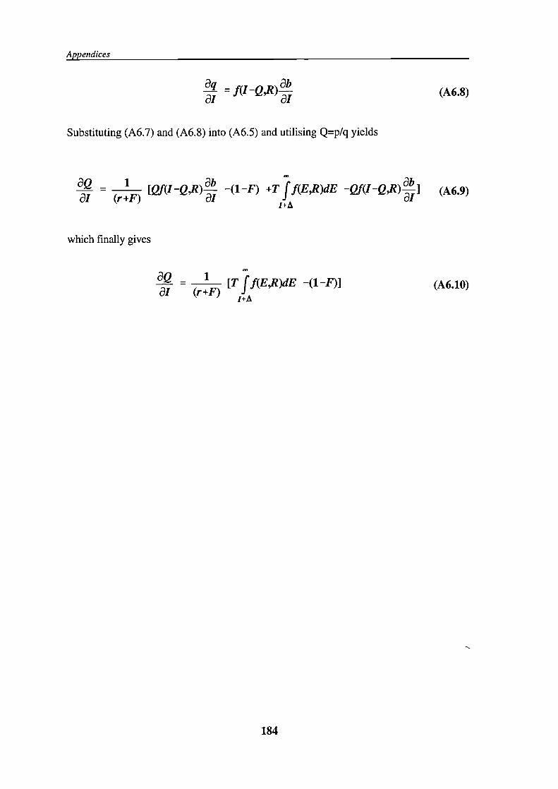
Appendices
- =f(I-Q,R)j?- (A6.8)
Substituting (A6.7) and (A6.8) into (A6.5) and utilising Q=p/q yields
aQ = 1 [Qf(I-Q,R)j?- -(1-F) +Tff(E,R)dE -Qf(I-Q,R)] (A6.9)ai (r+F)
which finally gives
= 1 [T ff(E,R)dE -(1-F)] (A6.1O)8i (r+F)
184

Appendices
APPENDIX 6.3 Derivation of the Optimality Condition; aviai
Define the value of the firm, V, as rn/n where
m =
f Ef(E,R)dE - f TEf(E,R)dE +
f TIf(E,R)dEJ-Q A6 11
+ f TAf(E,R)dE +f(L(1 -ic e -(1 -i)c 1) -C)f(E,R)dE
I+A -
n = r+F
(A6.12)
can then be written as
- 1[8m manl-
(A6.13)
In order to find V/3I one needs to first obtain both 3rn/31 and dV3i, which are derivedin the following (where b=I-Q) by use of the Leibnitz' rule.
= -(bY(b,R) +T(I+A)f(I+A,R) -TIf(I+A,R) + f Tf(E,R)dE
(A6.14)
- TAf(I+A,R) + (L(1-ic1-(1-i)c)-C)f(b,R)-
- =-bf(b,R) +T ff(E,R)dE +(L(1-ic-(1-i)c1-C)f(b,R).J?-) (A6.15)ai ai
I+A
and
185

Appendices
=f(b,R)PJ!
Substituting (6.15) and (6.16) into (6.13) yields the following result
31' = 13i (r+F)
+ f Tf(E,R)dE+(L(1-ic 1 -(1-i)c1)-C)f(b,R)-I = 0
(A6.16)
(A6.17)
which can also be written as (by using b=I-Q)
8V . 1 1 Tf(E,R)dE-f(b,R)-(D+I-(L(1-ic1-(1-i)c1)-C)bO3i (r+F)
Substituting b/3I and simplifying yields
av 1r+F f Tf(E,R)dEli-A
1+r - 1 Tf(E,R)dE)(D+I-(L(1-ic1-(1-i)c)C)] = 0r+F r+F
I-i-A
(A 6.18)
(A6.19)
since
al ai (A6.20)
and
1 [T ff(E,R)dE -(1 -F)]
31 (r+F)i-i-A
(A6.21)
as derived in Appendix 6.2.
186

Appendices
APPENDIX 6.4 The Sign of 82V1813R
It can be shown by differentiating equation (6.16) with respect to R that 82 V/BIBR is givenas the following
___ ___ ____ [Z]+a2v = 1 [(T 8f(E dE --f(b)(BC)[ 0F/8R310R r+F 0R r+F
-[Z][f'(b)(BC) ^f(b)]]
1Tf(Et?)dE]J
(A6.22)
where
0F= -f(b)
____
J 8R (A6.23)
= _1 [f(E-' f (1-I)(E-I)L()dEI+18R r+F
I-Q
+ f TdEQ af(E,R)
I^A I-Q
(A6.24)
8D . 1
-;i (r+F) [f(b)(BC)
- I (L(1_ic j_(1_ic)_Ci) tE+D f -jdE1
I -Q I-Q
(A6.25)
Since the sign of 8f(E,R)/8R is not known in different regions the effect of variability onborrowing is not unambigious.
187

Appendices
APPENDIX 7. Data
A.7.1 Construction of Variables:
The variables used in the estimation were measured as follows.
LeverageDependent variable of our model is measured as the ratio of long-term debt to the sum oflong-term debt and book value of equity (C 123). Long-term debt is calculated bysubtracting current liabilities (C 157) and shareholders' funds (C 132) from total liabilities(C157).
SizeSize is measured by the amount of total assets of firms.
Growth opportunitiesThe firm's growth opportunities are difficult to measure. As proxy, we used the followingmeasure
Growth= [(MVE + BVD)-BVA]/BVAwhere
MVE: market value of equity,BVD: book value of debtBVA: book value of assets.
This variable can be interpreted as the extra value capitalized by investors into firm valueover the present value of cash flows accruing from the firm's fixed assets. In this sense, itcan also be seen as investments in intangible assets that cannot be readily collateralized.Another alternative which has been widely used in the literature would be R&D expendituresof firms. Unfortunately, this item is rarely available in our data set, and hence we were notable to use it.
Non-debt tax shieldsIn much of the existing empirical work the sum of depreciation and amortization andinvestment credits is used as a proxy for non-debt tax shields. Unfortunately, in our dataset there were too many missing observations for these variables so that we could notemploy them. Instead, we used all other tax deductible expenses to approximate the non-debt tax shields. To do this the following equation is used
NDTS = Sales - (profit before tax) - (total interest)
188

Appendices
NDTS was then divided by total assets (Cl 15) to give the NDTS ratio.
ProfitabilityVarious measures have been used in the literature to measure the profitability as theprofitability of the firm. We measure the profitability as ratio of the earnings before interestand tax to the capital employed (net total assets). This ratio is given as
Profitability = EBITI Capital Employedwhere
EBIT: earnings before interest and tax (C34+C57)Capital employed: total assets (Cl 15) - total current liabilities (C 157)
LiquidityThe liquidity of the finn's assets is measured by the ratio of current assets (Cl 14) minusstocks (C105) to current liabilities (C157).
Operating leverageDegree of operating leverage (DOL) of the firm is constructed as
DOL = (% A in EBIT) / (% Li in Sales)
A.7.2 Sample Characteristics
As also explained in the text, only companies with at least five continuous time seriesobservations were selected. Our panel data set which includes 195 firms has the followingunbalanced structure:
Table A7.1 Structure of Panel
Number of records Number ofon each company companies
5 636 377 348 269 2010 911 6
189

Appendices
Table A7.2 lists the number of observations (companies) available in each year of the datasample.
Table A7.2. The Number of Companies in Each Year
Year Number of companies
1981 71982 271983 511984 821985 1151986 1571987 1941988 1921989 1901990 1861991 118
The industry groups have been reduced by regrouping them in the following eight SIC 1980one-digit industry classes. These industry classes are used as industry dummies in theestimation of our model.'
1. Energy and Water Supply Industries (SE Class 70);2. Manufacture of Chemicals (SE Class 68);3. Metal Goods, Engineering and Vehicle Industries (SE Classes 27, 33, 34, 35, 36, 41, 44,
69);4. Other Manufacturing Industries (SE Classes 11, 14, 19, 22, 28, 30, 31, 32, 37, 38, 39,
40, 45, 49, 52, 53, 54, 59, 62, 64, 65, 66, 67, 73, 95, 96);5. Construction (SE Class 18);6. Distribution, Hotels and Catering (SE Classes 13, 42, 47, 51, 56, 57, 58,)7. Transport and Communication (SE Class 71, 72, 74, 75)8. Other Services (SE Classes 21, 48, 90, 97).
The distribution of firms with respect to industry classes is given in Table A7.3.
1 Stock exchange classes are given in parenthesis. They correspond to the industrial classification used in EXSTAT,which are those allocated by the Stock Exchange and the Institute and Faculty of Actuaries.
190

Appendices
Table A7.3 The Number of Companies in Each Industry Class
Industry Class
Number of companies
1
52
13
534
735
206
147
148
15
A.7.3 Descriptive Statistics
Tables A7.4 and A7.5 give descriptive statistics and annual means of variables respectively.
Table A7.4 Descriptive Statistics
Variable
Mean (standard deviation)
levels
first differences
LeverageLeverage11SizeSize,1GrowthGrowth11NdtsNdts,1Profit1Liquidity
0.4670.4440.1320.1120.5860.7081.3051.3240.2541.144
(0.277)(0.273)(0.775)(0.688)(0.865)(0.974)(0.885)(0.904)(0.299)(1.151)
0.022 (0.175)0.029 (0.176)0.021 (0.110)0.0 19 (0.084)-0.122(0.828)-0.089 (0.861)-0.018 (0.392)-0.02 1 (0.399)-0.008 (0.255)0.017 (1.036)
191

Appendices
Table A7.5 Annual Means of Variables
Variable
LeverageSizeGrowthNDTSProfitabilityLiquidity
1981 1982 1983 1984 1985 1986 1987 1988 1989 1990 1991
0.30 0.28 0.34 0.40 0.41 0.39 0.40 0.44 0.49 0.51 0.500.01 0.01 0.04 0.04 0.05 0.05 0.09 0.12 0.15 0.17 0.220.80 0.56 0.52 0.78 0.96 0.74 0.83 0.91 0.62 0.60 0.261.41 1.24 1.31 1.28 1.44 1.42 1.38 1.32 1.28 1.34 1.290.27 0.21 0.19 0.23 0.20 0.26 0.29 0.31 0.28 0.24 0.210.92 1.49 1.02 1.10 1.07 1.23 1.14 1.12 1.06 1.03 1.16
It should be noted that annual means of variables cannot be strictly interpreted as trends inthe data since, as can be seen in Table A7.2, the structure of the data sample is unbalancedwhich means that the composition of companies changes over time.
192

REFERENCES

References
Aghion, P., Hart, 0. and Moore, J. (1992), "The Economics of Bankruptcy Reform",
The Journal of Law, Economics and Organization, Vol. 8, 523-546.
Aghion, P., Hart, 0. and Moore, J. (1993), "A Proposal for Bankruptcy Reform in
the UK", Insolvency Law and Practice, Vol. 9, 103-108.
Aivazian, V.A. and Callen, L.L. (1980), "Corporate Leverage and Growth. The Game-
Theoretic Issues", Journal of Financial Economics, Vol.8, 379-99.
Alderson, M.J. and Betker, B.L. (1995), "Liquidation Costs and Capital Structure", Journal
of Financial Economics, Vol.39, 45-69.
Altman, E.I. (1984), "A Further Empirical Investigation of the Bankruptcy Cost Question",
Journal of Finance, Vol.39, 1067-89.
Anderson, T.W. and Hsiao, C. (1982), "Formulation and Estimation of Dynamic Models
Using Panel Data", Journal of Econometrics, Vol. 18, 47-82.
Mg, J.S., Chua, J.H. and McConnell, J.J. (1982), "The Administrative Costs of Corporate
Bankruptcy: A Note", Journal of Finance, Vol.37, 337-48.
Arellano, M. and Bond, S. (1988), "Dynamic Panel Data Estimation Using DPD - A Guide
for Users", Institute for Fiscal Studies, Working Paper 88/15, London.
Arellano, M. and Bond, S. (1991), "Some Tests of Specification for Panel Data: Monte
Carlo Evidence and an Application to Employment Equations", The Review
of Economics Studies, Vol. 58, 277-297.
Asquith, P., Gertner, R. and Scharfstein, D.(1994), "Matomy of Financial Distress:An
Examination of Junk-Bond Issuers", The Quarterly Journal of Economics,
Vol.109, 625- 658.
194

References
Auerbach, A.J. (1985), "Real Determinants of Corporate Leverage", in B. Friedman, ed.,
Corporate Capital Structure in the United States, University of Chicago Press,
Chicago.
Balakrishnan, S. and Fox, I.(1993), "Asset Specificity, Firm Heterogeneity and Capital
Structure", Strategic Management Journal, Vol.14, 3-16.
Barclay, M.J. and Smith, C.W.(1995), 'The Maturity Structure of Corporate Debt", Journal
of Finance, Vol.50, 609-632.
Baxter, N.D. (1967), "Leverage, Risk of Ruin and the Cost of Capital", Journal of Finance,
Vol.22, 395-404.
Bayless, M.E. and Diltz, D. (1994), "Securities Offerings and Capital Structure Theory",
Journal of Business Finance and Accounting, Vol.21, 77-9 1.
Bergiof, E. And Thadden, E.L. (1994), "Short-term Versus Long-term Interests: Capital
Structure with Multiple Investors", Quarterly Journal of Economics, Vol.109, 1055-
1084.
Bergman, Y.Z. and Callen, J.F. (1991), "Opportunistic Underinvestment in the Debt
Renegotiation and Capital Structure", Journal of Financial Economics, Vol. 29,
137- 17 1.
Berlin, M. And Loeys, J. (1988), "Bond Covenants and Delegated Monitoring", Journal of
Finance, Vol.43, 397-412.
Blundell, R., Bond, S., Devereux, M. And Schiantarelli, F. (1992), "Investment and Tobin's
Q: Evidence from Company Panel Data", Journal of Econometrics, Vol. 51, 233-
257.
Bowen, R.M., Daley, L.A. and Huber C.C. (1982), "Evidence on the Existence and
195

References
Determinants of Inter-Industry Differences of Leverage", Financial Management,
Vol.11, 10-20.
Bradley, M., Jane!!, A. and Kim, E. (1984), "On the Existence of an Optima! Capital
Structure: Theory and Evidence", Journal of Finance, Vol.39, 857-80.
Brealey, R.A. and Myers, S.C. (1988), Principles of Corporate Finance, McGraw-Hill
Publishers.
Bulow, J.I. and Shoven, J.B. (1978), "The Bankruptcy Decision", The Bell Journal of
Economics, Vol.9, 437-56.
Campbell, C. and Underdown, B. (1991), Corporate Insolvency In Practice: An Analytical
Approach, Paul Chapman Publishing, London.
Castanias, R. (1983), "Bankruptcy Risk and Optimal Capita! Structure", Journal of Finance,
Vol.38, 1617-35.
Chemmanur, T.J. and Fulghieri, P. (1994a), "Reputation, Renegotiation and the Choice
between Bank Loans and Publicly Traded Debt", The Review of Financial
Studies, Vol.7, 475-506.
Chemmanur, T.J. and Fuighieri, P. (1994b), "Investment Bank Reputation, Information
Production, and Financial Intermediation", Journal of Finance, Vol.49, 57-79.
Chen, A.H. (1979), "A Theory of Corporate Bankruptcy and Optima! Capita! Structure",
in J.L. Bicksier ed., Handbook of Financial Economics, North Holland Publishing
Company.
Chowdhury, G., Green, C. and Miles D. (1994), "U.K. Companies' Short-term Financial
Decisions: Evidence from Company Accounts Data", The Manchester School, Vol.
62, 395-411.
196

References
Chung, K.H. (1993), "Asset Characteristics and Corporate Debt Policy: An Empirical Test",
Journal of Business Finance and Accounting, Vol.20, 83-98.
Chung, KS. and Smith, R.L. (1987), "Product Quality, Nonsalvageable Capital Investment
and the Cost of Financial Leverage", in Modern Finance and Indutrial Economics
ed. T.H. Copeland, Basil Blackwell, New York, 146-67.
Copeland, T.E. and Weston, J.F. (1988), Financial Theory and Corporate Policy, Addison-
Wesley.
Cornett, M. and Travlos, N. (1989), "Information Effects Associated with Debt-for-Equity
and Equity-for-Debt Exchange Offers", Journal of Finance, Vol.44, 452-68.
Cutler, D. and Summers, L. (1988), "The Costs of Conflict Resolution and Financial
Distress: Evidence from the Texaco-Pennzoil Litigations", Rand Journal of
Economics, Vol.19, 157-172.
DeAngelo, H. and Masulis, R.W. (1980), "Optimal Capital Structure Under Corporate and
Personal Taxation", Journal of Financial Economics, Vol.8, 3-29.
Diamond, D.W. (1984), "Financial Intermediation and Delegated Monitoring", Review of
Economic Studies, Vol.5 1, 393-414.
Diamond, D.W. (1989), "Reputation Acquisition in Debt Markets", Journal of Political
Economy, Vol.97, 828-862.
Diamond, D.W. (1991), "Monitoring and Reputation: The Choice between Bank Loans and
Directly Placed Debt", Journal of Political Economy, Vol.99, 689-721.
Fern, M.G. and Jones, W.H. (1979), "Determinant of Financial Structure: A New
Methodological Approach", Journal of Finance, Vol.34, 631-44.
197

References
Flath, D. and Knoeber, C.R. (1980), "Taxes, Failure Costs, and Optimal Industry Capital
Structure: An Empirical Test", Journal of Finance, Vol.35, 99-117.
Frankel, A.B. and Montgomery, J.D. (1991), "Financial Structure: An International
Perspective", Brookings Papers on Economic Activity, Vol.1, 257-310.
Franks, J.R. and Torous, W.N. (1992), "Lessons From a Comparison of US and UK
Insolvency Codes", Oxford Review of Economic Policy, Vol.3, 70-82.
Gertner, R. and Scharfstein, D. (1991), "A Theory of Workouts and the Effects of
Reorganization Law", Journal of Finance, Vol.46, 1189-1222.
Gilson, S., John, K. and Lang, L. (1990), "Troubled Debt Restructurings: An Empirical
Study of Private Reorganization of Firms in Default", Journal of Financial
Economics, Vol.26, 3 15-353.
Gordon R.H. (1985), "Comment", in B. Friedman, ed., Corporate Capital Structure in the
United States, University of Chicago Press, Chicago.
Harris, M. and Raviv, A. (1990), "Capital Structure and the Informational Role of Debt",
Journal of Finance, Vol.45, 32 1-49.
Harris, M. and Raviv, A. (1991), "The Theory of Capital Structure", Journal of Finance,
Vol.46, 297-355.
Harsanyi, J.C. and Selten, R. (1988), A General Theory of Equilibrium Selection in Games,
The MIT Press.
Haugen, R.A. and Senbet, L.W. (1978), "The Insignificance of Bankruptcy Costs to the
Theory of Optimal Capital Structure", Journal of Finance, Vol.33, 383-93.
Haugen, R.A. and Senbet, L.W. (1988), "Bankruptcy and Agency Costs: Their Significance
198

References
to the Theory of Optimal Capital Structure", Journal of Financial and Qualitative
Analysis, Vol.23, 27-38.
Homaifar, G., Zietz, J. and Benkato, 0. (1994), "An Empirical Model of Capital Structure:
Some New Evidence", Journal of Business Finance and Accounting, Vol.2 1, 1-14.
Hoshi, T., Kashyap, A., and Scharfstein, D. (1990), "The Role of Banks in Reducing the
Costs of Financial Distress in Japan", Journal of Financial Economics, Vol.27, 67-
88.
Hoshi, T., Kashyap, A., and Scharfstein, D. (1991), "Corporate Structure, Liquidity and
Investment: Evidence from Japanese Industrial Groups", Quarterly Journal of
Economics, Vol.106, 33-60.
Hsiao, C. (1985), "Benefits and Limitations of Panel Data", Econometric Reviews, Vol. 4,
121-174.
Jensen, M.C. (1986), "Agency Costs of Free Cash Flow, Corporate Finance and
Takeovers", American Economic Review, Vol.76, 323-39.
Jensen, M.0 and Meckling, W. (1976), "Theory of the Firm Managerial Behaviour, Agency
Costs, and Capital Structure", Journal of Financial Economics, Vol.3, 305-60.
John, K. and Nachman, D.C. (1985), "Risky Debt, Investment Incentives, and Reputation
in a Sequential Equilibrium", Journal of Finance, Vol.40, 863-880.
Keasey, K. and Watson, R. (1994), "The Bank Financing of Small Firms in UK: Issues and
Evidence", Small Business Economics, Vol.6, 349-362.
Kim, E. (1978), "A Mean-Variance Theory of Optimal Capital Structure and Corporate
Debt Capacity", Journal of Finance, Vol.33, 45-63.
199

References
Kim, W.S. and Sorensen, E.H. (1986), "Evidence on the Impact of the Agency Costs of
Debt on Corporate Debt Policy", Journal of Financial and Qualitative Analysis,
Vol.21, 131-44.
Kraus, A. and Litzenberger, R. (1973), "A State-Preference Model of Optimal Financial
Leverage", Journal of Finance, Vol.28, 911-22.
Kreps, D. and Wilson, R. (1982), "Reputation and Imperfect Information", Journal of
Economic Theory, Vol.27, 257-79.
Leland, H. and Pyle, D. (1977), "Informational Asymmetries, Financial Structure and
Financial Intermediation", Journal of Finance, 32, 37 1-387.
Long, M. and Malitz, I. (1985), "The Investment Financing Nexus: Some Empirical
Evidence", Midland Corporate Finance Journal, Vol.3, 53-59.
Lys, T. and Sivaramakrishman, K. (1988), "Earnings Expectations and Capital
Restructuring: The Case of Equity-for-Debt Swaps", Journal of Accounting
Research, Vol.26, 273-99.
Maddala, G.S. (1989), Introduction to Econometrics, Macmillan Publishers, New York.
Maksimovic, V. and Titman, S. (1991), "Financial Policy and Reputation for Product
Quality", Review of Financial Studies, Vol.4, 175-200.
Marsh, P. (1982), "The Choice Between Equity and Debt", Journal of Finance, Vol.37,
121-44.
Milgrom, P. And Roberts, J. (1982), "Predation, Reputation and Entry Deterence", Journaj
of Economic Theory, Vol.27, 280-3 12.
Miller, M.H. (1977), "Debt and Taxes", Journal of Finance, Vol.32, 261-75.
200

References
Modigliani, F. and Miller, M.H. (1958), "The Cost of Capital, Corporation Finance and the
Theory of Investment", American Economic Review, Vol.48, 26 1-97.
Modigliani, F. and Miller, M.H. (1963), "Corporate Income Taxes and the Cost of
Capital A Correction", American Economic Review, Vol.53, 433-43.
Myers, S.C. (1977), "Determinants of Corporate Borrowing", Journal of Financial
Economics, Vol.5, 147-75.
Myers, S.C. (1984), "The Capital Structure Puzzle", Journal of Finance, Vol.39, 575-92.
Myers, S.C. and Majiuf, N.S. (1984), "Corporate Financing and Investment Decisions When
Firms Have Information that Investors Do Not Have", Journal of Financial
Economics, Vol.13, 187-221.
Ofek, E. (1993), "Capital Structure and Firm Response to Poor Performance: Empirical
Evidende", Journal of Financial Economics, Vol.34, 3-30.
Pesaran, M. and Smith, R. (1994), "Estimating Long-run Relationships from Dynamic
Heterogenous Panels", Mimeo, University of Cambridge.
Prowse, S.D. (1991), "Institutional Investment Patterns and Corporate Financial Behaviour
in the U.S. and Japan", Journal of Financial Economics, Vol. 27, 43-66.
Rajan, R. (1992), "Insiders and Outsiders: The Choice between Relationship and Arms
Length Debt", Journal of Finance, Vol.47, 1367-1399.
Rajan R.G. and Zingales, L. (1995), "What Do We Know About Capital Structure? Some
Evidence from International Data", Journal of Finance, Vol.50, 142 1-1460.
Ross, S. (1977), "The Determination of Financial Structure: The Incentive Signalling
Approach", Bell Journal of Economics, Vol.8, 23-40.
201

References
Scott, J.H. (1976), "A Theory of Optimal Capital Structure", Bell Journal of Economics,
Vol.7, 33-54.
Sharpe, S. (1990), "Asymmetric Information, Bank Lending and Implicit Contracts: A
Stylized Model of Customer Relationships", Journal of Finance, Vol.45, 1069-1087.
Shleifer, A. and Vishny, R.W. (1992), "Liquidation Values and Debt Capacity: A Market
Equilibrium Approach", Journal of Finance, Vol.47, 1343-1366.
Stiglitz, J.E. (1969), "A Re-Examination of the Modigliani-Miller Theorem", American
Economic Review, Vol.59, 784-93.
Stiglitz, J.E. (1972), "Some Aspects of the Pure Theory of Corporate Finance: Bankruptcies
and Takeovers", Bell Journal of Economics and Management Science, Vol.3,
458-82.
Stiglitz, J.E. (1974), "On the Irrelevance of Corporate Financial Policy", American
Economic Review, Vol.64, 85 1-66.
Stulz, R. (1988), "Managerial Control of Voting Rights: Financing Policies and the Market
for Corporate Control", Journal of Financial Economics, Vol.20, 25-54.
Stulz, R. (1990), "Managerial Discretion and Optimal Financing Policies", Journal of
Financial Economics, Vol.26, 3-27.
Sydseter, K. and Hammond, P.J. (1995), Mathematics for Economic Analysis, Prentice
Hall, New Jersey.
Thakor, A.V. and Wilson, P.F. (1995), "Capital Requirements, Loan Renegotiation and the
Borrower's Choice of Financing Source, Journal of Banking and Finance, Vol.19,
693-711.
202

References
Titman, S. (1984), "The Effect of Capital Structure on a Firm's Liquidation Decision",
Journal of Financial Economics, Vol.13, 137-5 1.
Titman, S. and Wessels, R. (1988), "The Determinants of Capital Structure Choice",
Journal of Finance, Vol.43, 1-19.
Warner, J.B. (1977), "Bankruptcy Costs: Some Evidence", Journal of Finance, Vol.32,
337-48.
Webb, D.C. (1987a), "The Importance of Incomplete Information in Explaining the
Existence of Costly Bankruptcy", Economica, Vol.54,279-88.
Webb, D.C. (1987b), "Conflict of Interest, Bond Rating and the Value Maximization Rule",
Economica, Vol.54, 455-63.
Webb, D.C. (1991), "An Economic Evaluation of Insolvency Procedures in the United
Kingdom: Does the 1986 Insolvency Act Satisfy the Creditor's Bargain", Oxford
Economic Papers, Vol.43, 139-157.
Weiss, L.A. (1990), "Bankruptcy Resolution-Direct Costs and Violation of Priority Claims",
Journal of Financial Economics, Vol.27, 285-314.
White, M.J. (1980), "Public Policy Toward Bankruptcy: Me-First and Other Priority Rules",
Bell Journal of Economics, Vol.11, 550-64.
White, M.J. (1983), "Bankruptcy Costs and the New Bankruptcy Code", Journal of
Finance, Vol.3 8, 477-88.
White, M.J. (1989), "The Corporate Bankruptcy Decision", Journal of Economic
Perspectives, Vol.3, 129-5 1.
203

References
Williamson, 0. (1988), "Corporate Finance and Corporate Governance", Journal of
Finance, Vol.43, 567-59 1.
204