couette flow
DESCRIPTION
The presentation about Coutte FlowTRANSCRIPT


Group Members
Number Name Registration Number
1 Khawar Shahzad ME 113 009
2 Muhammad Ali ME 113 115
3 Mohsin Raza ME 113 080
4 Zohaib Ahmad ME 113 022
5 Aoun Abbas ME 113 074
6 Omer Ayub ME 113 089
7 Muhammad Ramzan ME 113 100
8 Khuram Yousaf ME 113 107
9 Zain Talib ME 113 108
10 Hassan Aamir ME 113 053
11 Adeel Anwar ME 113 039
2

Introduction
http://upload.wikimedia.org/wikipedia/commons/thumb/9/93/Laminar_shear.svg/800px-Laminar_shear.svg.png
3

Introduction
Laminar
Viscous
Incompressible Fluid
4
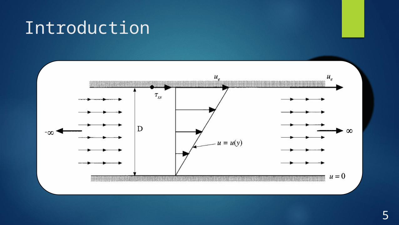
Introduction
5

Analytical Solution
The governing y-direction momentum equation is:
𝛒 𝛛 𝐯𝛛 𝐭
+𝛒𝐮 𝛛𝐯𝛛𝐱
+𝛒𝐯 𝛛 𝐯𝛛 𝐲
+𝛒𝐰 𝛛 𝐯𝛛𝐳
=− 𝛛𝐩𝛛𝐲
+𝛛𝛕𝐱𝐲
𝛛𝐱+𝛛𝛕𝐲𝐲
𝛛 𝐲+𝛛𝛕𝐳𝐲
𝛛𝐳+𝛒𝐟 𝐲
Steady State Assumption No Body Forces
𝟎=𝛛𝐩𝛛𝐲
6
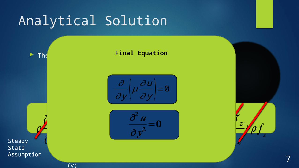
Analytical Solution
The governing x-direction momentum equation is:
𝛒 𝛛𝐮𝛛𝐭
+𝛒𝐮 𝛛𝐮𝛛𝐱
+𝛒 𝐯 𝛛𝐮𝛛 𝐲
+𝛒𝐰 𝛛𝐮𝛛𝐳
=− 𝝏𝒑𝝏 𝒙
+𝝏𝝉𝒙𝒙
𝝏𝒙+𝝏𝝉 𝒚𝒙
𝝏 𝒚+𝝏𝝉𝒛𝒙
𝝏𝒛+𝝆 𝒇 𝒙
Steady State Assumption Y-Direction
Velocity (v) is Zero
No beginning or end of this flow in x-direction
Final Equation
𝜕𝜕 y ( μ 𝜕u𝜕 y )=0
𝛛𝟐𝒖𝛛𝐲𝟐=𝟎
7

Using boundary condition at we have, we get.
Using boundary condition at we have, we get.
𝒖𝒖𝒆
=𝒚𝑫
Analytical Solution
8

Analytical Solution – Matlab Codeclcclear%Workspace and Command History Cleared
ue = 0.01 %Velocity of Upper Plate moving with 0.01m/s
D = 0.05 %Separation Distance between plate. 5cm%y is distance from lower plate to upper plate
y = linspace(0,D,500);for i=1:1:500 U(i)=(ue*y(i))/D;endplot (y,U)legend ('Couette Flow Velocity Profile','Fontsize',12')xlabel ('Width Between Plates (m)',' Fontsize ',12')ylabel ('Velocity Profile (m/s)',' Fontsize ',12')axis ([-0.01 0.06 -0.001 0.012])
-0.01 0 0.01 0.02 0.03 0.04 0.05 0.06
0
2
4
6
8
10
12x 10
-3
Width Between Plates (m)
Ve
locity P
rofile
(m
/s)
Couette Flow Velocity Profile
9

Numerical Implicit Method
Nature of Partial Differential Equation
Parabolic Nature Equation because
Conclusion: Time Marching Possible
10

The Numerical Formulation
11

The Numerical Formulation
12

The Numerical Formulation
𝐮 𝐣𝐧+𝟏=𝐮 𝐣
𝐧+𝚫𝐭
𝟐 (𝚫𝐲 )𝟐𝐑𝐞𝐃
𝐮 𝐣+𝟏𝐧+𝟏+
𝚫𝐭𝟐 (𝚫 𝐲 )𝟐𝐑𝐞𝐃
𝐮 𝐣+𝟏𝐧 −
𝚫𝐭𝟐 (𝚫𝐲 )𝟐𝐑𝐞𝐃
𝟐𝐮 𝐣𝐧+𝟏−
𝚫𝐭𝟐 (𝚫𝐲 )𝟐𝐑𝐞𝐃
𝟐𝐮 𝐣𝐧+
𝚫𝐭𝟐 (𝚫𝐲 )𝟐𝐑𝐞𝐃
𝐮 𝐣−𝟏𝐧+𝟏+
𝚫𝐭𝟐 (𝚫 𝐲 )𝟐𝐑𝐞𝐃
𝐮 𝐣−𝟏𝐧
13

The Numerical Formulation
A B 𝐊 𝐣
𝐀𝐮 𝐣− 1𝐧+1+𝐁𝐮 𝐣
𝐧+1+𝐀𝐮 𝐣+1𝐧+1=𝐊 𝐣
14

The Numerical Formulation
𝐀𝐮 𝐣− 1𝐧+1+𝐁𝐮 𝐣
𝐧+ 1+𝐀 𝐮 𝐣+1𝐧+1=𝐊 𝐣
[¿𝐁¿𝐀¿𝟎¿𝟎¿𝟎
¿𝐀¿𝐁¿𝐀¿𝟎¿𝟎
¿𝟎¿𝐀¿𝐁¿𝐀¿𝟎
¿𝟎¿𝟎¿𝐀¿𝐁¿𝐀
¿𝟎¿𝟎¿𝟎¿𝐀¿𝐁
] [¿𝐮𝟐
𝐧+𝟏
¿𝐮𝟑𝐧+𝟏
¿𝐮𝟒𝐧+𝟏
¿𝐮𝟓𝐧+𝟏
¿𝐮𝟔𝐧+𝟏
]=[¿𝐊 𝟐−𝐀 𝐮𝟏
𝐧+𝟏
¿𝐊𝟑
¿𝐊𝟒
¿𝐊𝟓
¿𝐊𝟔
¿𝐊 𝟔−𝐀 𝐮𝟕𝐧+𝟏
]15

Thank you!
16