coulomb stress accumulation along the san andreas · pdf filecoulomb stress accumulation along...

Coulomb stress accumulation along the San Andreas Fault system

Bridget Smith and David SandwellInstitute for Geophysics and Planetary Physics, Scripps Institution of Oceanography, La Jolla, California, USA

Received 2 August 2002; revised 16 January 2003; accepted 18 February 2003; published 11 June 2003.

[1] Stress accumulation rates along the primary segments of the San Andreas Fault systemare computed using a three-dimensional (3-D) elastic half-space model with realistic faultgeometry. The model is developed in the Fourier domain by solving for the response ofan elastic half-space due to a point vector body force and analytically integrating theforce from a locking depth to infinite depth. This approach is then applied to the SanAndreas Fault system using published slip rates along 18 major fault strands of the faultzone. GPS-derived horizontal velocity measurements spanning the entire 1700 � 200 kmregion are then used to solve for apparent locking depth along each primary fault segment.This simple model fits remarkably well (2.43 mm/yr RMS misfit), although somediscrepancies occur in the Eastern California Shear Zone. The model also predicts verticaluplift and subsidence rates that are in agreement with independent geologic and geodeticestimates. In addition, shear and normal stresses along the major fault strands are used tocompute Coulomb stress accumulation rate. As a result, we find earthquake recurrenceintervals along the San Andreas Fault system to be inversely proportional to Coulomb stressaccumulation rate, in agreement with typical coseismic stress drops of 1–10 MPa. This 3-Ddeformation model can ultimately be extended to include both time-dependent forcing andviscoelastic response. INDEX TERMS: 1206 Geodesy and Gravity: Crustal movements—interplate

(8155); 1242 Geodesy and Gravity: Seismic deformations (7205); 3210 Mathematical Geophysics: Modeling;

8164 Tectonophysics: Stresses—crust and lithosphere; 8199 Tectonophysics: General or miscellaneous;

KEYWORDS: San Andreas Fault, Coulomb stress, crustal deformation, SCEC velocities, crustal stress

Citation: Smith, B., and D. Sandwell, Coulomb stress accumulation along the San Andreas Fault system, J. Geophys. Res., 108(B6),

2296, doi:10.1029/2002JB002136, 2003.

1. Introduction

[2] The San Andreas Fault (SAF) system, spanning over1700 km from the Mendocino Triple Junction in the north tothe Gulf of California in the south, defines the complextectonic boundary between the Pacific and North Americanplates. As the two plates slide past each other, the SAFsystem accommodates �35–50 mm/yr of relative platemotion that is distributed across a 200 km wide zone[Working Group on California Earthquake Probabilities(WGCEP), 1995, 1999]. The SAF system is composed ofan intricate network of subfaults, each of varying geometry,locking depth, and associated failure properties. Earthquakerecurrence intervals also vary dramatically along the SAFsystem subfaults, ranging from 20 years to over 300 years.In order to better understand the earthquake cycle and alsohelp constrain faulting models of the San Andreas Faultsystem, geodetic measurements of interseismic, postseismic,and coseismic deformation are continually collected alongthe entire North American-Pacific plate boundary.[3] While many previous studies of the SAF region have

developed local fault slip models to match regional geodeticobservations of surface displacement [Savage and Burford,1973; Savage et al., 1979; King et al., 1987; Li and Lim,

1988; Eberhart-Phillips et al., 1990; Savage, 1990; Lisowskiet al., 1991; Feigl et al., 1993; Savage and Lisowski, 1993;Freymueller et al., 1999; Burgmann et al., 2000;Murray andSegall, 2001], our objectives are somewhat different in thatwe investigate the steady state behavior of the entire SanAndreas Fault system. By constraining relative plate motion,maintaining appropriate fault geometry, and implementinggeodetic measurements spanning the entire system, weare able to model three-dimensional (3-D) deformation andcalculate stress accumulation. First, we investigate whether asingle far-field plate velocity can be partitioned amongparallel strands in order to accurately model near-field geo-detic measurements. Second, we establish spatial variationsin apparent locking depth along the main segments of theSAF system. Finally, we use our model to estimate secularbuildup in Coulomb stress within the seismogenic layer andaccumulation of scalar seismic moment.[4] The primary purpose for developing our model is to

estimate Coulomb stress accumulation rate and to exploreits relevancy to earthquake occurrence and failure potential.Following the assumption that major earthquakes typicallyproduce stress drops on the order of 1–10 MPa, estimatesof Coulomb stress accumulation rate can provide an upperbound on the recurrence interval of a particular fault seg-ment. Furthermore, recent studies of induced Coulombstress changes propose that earthquakes may be triggeredby stress changes as small as 0.1 MPa [King et al., 1994;

JOURNAL OF GEOPHYSICAL RESEARCH, VOL. 108, NO. B6, 2296, doi:10.1029/2002JB002136, 2003

Copyright 2003 by the American Geophysical Union.0148-0227/03/2002JB002136$09.00

ETG 6 - 1

Stein et al., 1994; Fialko and Simons, 2000; King andCocco, 2001; Zeng, 2001]. High Coulomb stress accumu-lation rate has also been linked to areas of surface creep[Savage and Lisowski, 1993]. A better understanding ofsuch stress release processes at major plate boundaries,along with estimates of seismic moment magnitude, havealso been the focus of recent earthquake hazard potentialstudies [WGCEP, 1995, 1999; Working Group on NorthernCalifornia Earthquake Potential (WGNCEP), 1996]. In thisanalysis, we inspect the role of locking depth, fault geom-etry, and paralleling fault strands on accumulating inter-seismic stress along San Andreas Fault system, andinvestigate how such accumulation is related to shallowfault creep, earthquake recurrence interval, and seismicmoment accumulation.

2. Fourier Solution to 3-D Body Force Model

[5] For the last several decades, the most commonly usedanalytic models of fault-induced deformation have beenbased on the dislocation solutions of Chinnery [1961,1963], Rybicki [1973], and Okada [1985, 1992]. The latterprovide analytic expressions for stress, strain, and displace-ment in an elastic half-space due to a displacement dis-continuity. While these dislocation models are accurate andcomputationally efficient when applied to individual faultsor small fault systems, they may become computationallyprohibitive when representing fault geometry over the entireNorth American-Pacific plate boundary. For example, 4 �105 model calculations are required for 1000 GPS measure-ments and 400 fault patches. Modeling of InSAR observa-tions could easily require 4 � 109 model calculations.However, if model calculations are performed in the spectraldomain, the computational effort is substantially reduced.Rather than calculate the Fourier transform of the analyticsolutions mentioned above, we instead solve the 3-Delasticity equations in the wave number domain and theninverse Fourier transform to obtain space domain solutions.The key elements of our model derivation are summarizedin Appendix A. In the two-dimensional case, our modelmatches the classical arctangent solution of Weertman[1964], both analytically and numerically (Appendix A).While this elastic half-space model currently ignores crustalheterogeneities and does not explicitly incorporate non-elastic rheology below the brittle-ductile transition, it pro-duces reasonable estimates of first-order tectonic featurescomparable to other simple models [Savage and Burford,1973].[6] To summarize our analytic approach (Appendix A),

the elasticity equations are used to derive a set of transferfunctions (in the wave number domain) for the 3-D dis-placement of an elastic half-space due to an arbitrarydistribution of vector body forces. The numerical compo-nents of this approach involve generating a grid of forcecouples that simulate complex fault geometry, taking the 2-DFourier transform of the grid, multiplying by the appropriatetransfer function, and finally inverse Fourier transforming.The force model must be designed to match the velocitydifference across the plate boundary and have zero net forceand zero net moment. There is a similar requirement ingravity modeling, where mass balance is achieved byimposing isostatic compensation and making the grid

dimensions several times larger than the longest lengthscale in the system (e.g., flexural wavelength or lithosphericthickness). For this fault model, the characteristic lengthscale is the locking depth of the fault. The key is toconstruct a model representing a complicated fault systemwhere the forces and moments are balanced. Our numericalapproach is as follows:[7] 1. Develop a force couple segment from the analytic

derivative of a Gaussian approximation to a line segment asdescribed in Appendix A; this ensures exact force balance.For an accurate simulation, the half width of the Gaussianmust be greater than the grid size but less than the lockingdepth.[8] 2. Construct a complicated force couple model using

digitized fault segments. For each segment, the strength ofthe couple is proportional to the long-term slip rate on thefault segment and the direction of the couple is parallel tothe overall plate boundary direction (not the local faultdirection). This simulates the far-field plate tectonic forcecouple. Because the model has force couples, the vectorsum of all of the forces in the model is zero but there is alarge unbalanced moment because all of the force couplesact in the same direction.[9] 3. Double the grid size and place a mirror image of

the force couple distribution in the mirror grid so that themoment due to the image fault exactly balances the momentdue to the real fault. Following these steps, we combineboth analytic and numeric approaches to elastic fault mod-eling for analysis of the San Andreas Fault system.

3. Modeling the San Andreas Fault Zone

[10] We apply our semianalytic model (Appendix A) tothe geometrically complex fault setting of the SAF system.After digitizing the major fault strands along the SAFsystem from geologic maps [Jennings, 1994] into over400 elements, we group the elements into 18 fault segmentsspatially consistent with previous geologic and geodeticstudies (Figure 1). Fault segments include the followingregions: (1) Imperial, (2) Brawley (defined primarily byseismicity [Hill et al., 1975] rather than by mapped surfacetrace), (3) Coachella Valley-San Bernardino Mountains, (4)Borrego (includes Superstition Hills and Coyote Creekregions), (5) Anza-San Jacinto (includes San BernardinoValley), (6) Mojave, (7) Carrizo, (8) Cholame, (9) ParkfieldTransition, (10) San Andreas creeping, (11) Santa CruzMountains-San Andreas Peninsula, (12) San Andreas NorthCoast, (13) South Central Calaveras, (14) North Calaveras-Concord, (15) Green Valley-Bartlett Springs, (16) Hayward,(17) Rodgers Creek, and (18) Maacama. The fault system isrotated about its pole of deformation (52�N, 287�W) into anew coordinate system [Wdowinski et al., 2001], and faultsegments are embedded in a 1-km grid of 2048 elementsalong the SAF system and 1024 elements across the system(2048 across including the image). We assume that thesystem is loaded by stresses extending far from the lockedportion of the fault and that locking depth and slip rateremain constant along each fault segment.[11] Each of the 18 SAF segments is assigned a deep

slip rate based on geodetic measurements, geologic offsets,and plate reconstructions [WGCEP, 1995, 1999]. In somecases, slip rates (Table 1) were adjusted (±5 mm/yr on

ETG 6 - 2 SMITH AND SANDWELL: COULOMB STRESS ALONG THE SAN ANDREAS FAULT

average) in order to satisfy an assumed far-field platevelocity of 40 mm/yr. This constant rate simplifies the modeland, as we show below, it has little impact on the near-fieldvelocity, strain rate, and Coulomb stress accumulation rate.Moreover, it provides a remarkably good fit to the geodetic

data, except in the Eastern California Shear Zone, wheremisfit is expected due to omission of faults in this area.Because slip estimates remain uncertain for the Maacamaand Bartlett Springs segments, we assume that these seg-ments slip at the same rates as their southern extensions, theRodgers Creek and Green Valley faults, respectively.[12] After assigning these a priori deep slip rates, we

estimate lower locking depth for each of the 18 fault seg-ments using a least squares fit to 1099 GPS-derived hori-zontal velocities. Geodetic data for the southern SAF region,acquired between 1970 and 1997, were provided by theCrustal Deformation Working Group of the Southern Cal-ifornia Earthquake Center (SCEC) (D. Agnew, SCEC,Horizontal deformation velocity map version 3.0, personalcommunication, 2002) GPS velocities for the Calaveras-Hayward region were provided by the U.S. GeologicalSurvey, Stanford University, and the University of Califor-nia, Berkeley and reflect two data sets, one of campaignmeasurements (1993–1999) and one of BARD networkcontinuous measurements. Data used to model the northernregion of the SAF system were obtained from Freymeuller etal. [1999] and represent campaign measurements from 1991to 1995. These four geodetic data sets combine to a total of1099 horizontal velocity vectors spanning the entire SanAndreas Fault zone (Figure 2a).

4. Geodetic Inversion

[13] The relationship between surface velocity and lock-ing depth is nonlinear, thus we estimate the unknown depthsof the 18 locked fault segments using an iterative, leastsquares approach based on the Gauss-Newton method. Wesolve the system of equations Vgps(x, y) = Vm(x, y, d), whereVgps is the geodetic velocity measurement, Vm is themodeled velocity, and d is the set of locking depth param-eters that minimize the weighted residual misfit c2. Thedata misfit is

V ires ¼

V igps � V i

m

sið1Þ

c2 ¼ 1

N

XNi¼1

V ires

� �2 ð2Þ

Figure 1. (opposite) San Andreas Fault system segmentlocations in the pole of deformation (PoD) coordinatesystem over shaded regional topography. Fault segmentscoinciding with Table 1 are (1) Imperial, (2) Brawley, (3)Coachella Valley-San Bernardino Mountains, (4) Borrego,(5) Anza-San Jacinto, (6) Mojave, (7) Carrizo, (8) Cholame,(9) Parkfield Transition, (10) San Andreas creeping, (11)Santa Cruz Mountains-San Andreas Peninsula, (12) SAFNorth Coast, (13) South Central Calaveras, (14) NorthCalaveras-Concord, (15) Green Valley-Bartlett Springs, (16)Hayward, (17) Rodgers Creek, and (18) Maacama. We usethe pole of deformation (PoD) of Wdowinski et al. [2001](52�N, 287�W) and note that the longitude axis has beenshifted in order to place 0� in the center of the grid. Dashedlines represent horizontal corridor sections, bounded byfault segments, constrained to total 40 mm/yr.

SMITH AND SANDWELL: COULOMB STRESS ALONG THE SAN ANDREAS FAULT ETG 6 - 3

where si is the uncertainty estimate of the ith geodeticvelocity measurement and N is the number of geodeticobservations. Uncertainties in each measurement are used toform the diagonal covariance matrix of the data.[14] The modeled velocity, Vm, is expanded in a Taylor

series about an initial locking depth, d

Vm dþ�½ ¼ Vm d½ þXMj¼1

�j

@Vm

@djþ . . . ð3Þ

where �j is a small perturbation to the jth depth parameter.Partial derivatives are computed analytically using thepreintegrated body force solution (Appendix A). BecauseVm[d + �] is an approximation to the observed velocity,Vgps, the residual velocity may be expressed as the depthperturbation � times the matrix of partial derivatives DVm

Vres ¼ DVm�: ð4Þ

The model perturbation is then calculated using the standardweighted least squares approach

� ¼ DVTmC

�1DVm

� ��1DVT

mC�1Vres ð5Þ

where C is the diagonal covariance matrix of measurementuncertainties. Because of the nonlinear aspects of theinversion, a step length damping scheme is used for eachiteration, k,

dkg ¼ dk�1 þ g� 0 < g < 1 ð6Þ

where g is the damping parameter [Parker, 1994]. Dampingparameter g is chosen such that

c2 mg

� �¼ c2 mk½ � 2gc2 mk½ þ o k g� k ð7Þ

will guarantee a smaller misfit than c2[mk]. The best fit isobtained by cautiously repeating this algorithm until all 18locking depth solution parameters converge. Uncertainties

in estimated locking depths are determined from thecovariance matrix of the final iteration.

5. Results

5.1. Horizontal Motion and Locking Depth

[15] Our locking depth inversion involves 26 free param-eters: two unknown velocity components for each of the fourGPS networks and 18 locking depths (Figures 1 and 2). Theunknown velocity component for each of the GPS data setsis estimated by removing the mean misfit from a startingmodel (uniform locking depth of 10 km). The initial RMSmisfit with respect to the starting model is 5.31 mm/yr(unweighted). After 10 iterations, the RMS misfit improvesto 2.43 mm/yr (Figure 2). Comparisons between GPS dataand fault-parallel modeled velocities for twelve fault corri-dors are shown in Figure 2b. Each model profile is acquiredalong a single fault-perpendicular trace, while the geodeticmeasurements are binned within the fault corridors andprojected onto the perpendicular trace, thus some of thescatter is due to projection of the data onto a common profile.[16] Locking depth inversion results (Table 1) are primar-

ily dependent on data acquired near the fault trace. Uncer-tainties in these estimates (1s standard deviation) arerelatively low in the southern portion of the SAF systemwhere there is a high density of GPS stations. In contrast,uncertainties are much higher along the northern segmentswhere there is a relatively low density of GPS stations. Ourdepth solutions are generally consistent with previouslypublished locking depths and distributions of seismicity[Savage, 1990; Johnson et al., 1994; Feigl et al., 1993;Freymueller et al., 1999]. Again, we emphasize that theseare apparent locking depths since we have not included theviscoelastic response of the earth to intermittent earthquakes[Thatcher, 1983]. A more detailed discussion of modelcharacteristics and GPS agreement for each of the 18 faultsegments is provided in Appendix B.

5.2. Far-Field Constraint: 40 mm///yr

[17] Because we are primarily interested in stress behaviorclose to the fault, the magnitude of the far-field velocity is

Table 1. San Andreas Fault System Parameters and Results

Segment NameSlip,a

mm/yrLockingDepth, km s,b km

Coulomb Stress,MPa/100 years

Moment Rate, N m/100years per km � 1014 tr,

a years

1 Imperial 40 5.9 1.20 10.0 7.1 402 Brawley Seismic Zone 36 6.3 1.30 8.5 6.8 243 Coachella-San Bernardino Mountains 28 22.6 1.70 1.7 19.0 1464 Borrego 4 2.0 7.70 0.5 0.2 1755 Anza-San Jacinto 12 13.1 2.30 1.7 4.7 836 Mojave 40 26.0 1.70 0.6 31.2 1507 Carrizo 40 25.2 2.60 1.6 30.2 2068 Cholame 40 12.7 2.40 4.0 15.2 1409 Parkfield Transition 40 14.5 2.90 4.0 17.4 2510 San Andreas Creeping 40 1.3 0.20 n/a 1.6 n/a11 Santa Cruz-Peninsula 21 9.3 0.60 3.2 5.9 40112 San Andreas North Coast 25 19.4 2.10 2.3 14.6 75913 South-Central Calaveras 19 1.6 0.20 12.5 0.9 7514 North Calaveras-Concord 7 13.7 4.60 1.1 2.9 70115 Green Valley-Bartlett Springs 5 9.1 8.40 1.2 1.4 23016 Hayward 12 15.7 3.70 1.5 5.7 52517 Rodgers Creek 12 18.9 6.70 1.1 6.8 28618 Maacama 10 12.3 4.30 1.7 3.7 220aWGCEP [1995, 1999] and WGNCEP [1996].bLocking depth uncertainty.


not the most critical parameter in our analysis. Nevertheless,we attempt to justify the usage of a single far-field rate of40 mm/yr for the entire SAF system. The full NorthAmerica-Pacific plate motion is approximately 46 mm/yr[DeMets et al., 1990, 1994]. While the San Andreas Faultsystem accommodates the majority of deformation occurringbetween the two plates, substantial regions of deformationalso exist far from the SAF system [Minster and Jordan,1987; Ward, 1990]. These regions include the EasternCalifornia Shear Zone, the Sierra Nevada-Great Basin shearzone, the Garlock fault zone, the Owens Valley Faults zoneand the San Jacinto, Whittier-Elsinore, Newport-Inglewood,Palos Verdes, and San Clemente faults. Partitioning detailsof the total slip rate remain uncertain. The WGCEP [1995,1999] propose a total slip rate of 36–50 mm/yr along thenorthern portion of the San Andreas Fault system and a rateof 35 mm/yr along the southern portion of the San AndreasFault system. In this analysis, we adopt a constant far-fieldvelocity of 40 mm/yr for both northern and southern portionsof the SAF system. Our results, using realistic fault geometryand variable locking depth, provide an adequate fit to all of

the data (Figure 2b), especially close to the fault zones wherewe wish to calculate stress accumulation. The far-fieldregions of the extreme southern and northern SAF systemare underestimated by our model (Figure 2b, profiles 1–4,11, 12), while the middle portions of the system are wellmatched in the far field (Figure 2b, profiles 6, 7, 9). There issignificant misfit on the eastern sides of profiles 3, 4, and 5,which reflect both coseismic and interseismic shear in theMojave desert. The apparent locking depth along theseprofiles may be artificially high in order to minimize themisfit in the Eastern California Shear Zone. Nevertheless, wehave found that increasing the far-field velocity to 45 mm/yr,for example, does not significantly improve the fit to theGPS data and yields long-term slip rates that are inconsistentwith published estimates [WGCEP, 1995, 1999]. Overall, thematch to the GPS data is quite good considering thesimplicity of the model.

5.3. Vertical Motion

[18] An intuitive yet important aspect of our 3-D model isthe vertical component of deformation (Figure 3), driven

Figure 2. (a) Fault-parallel velocity map of best fitting model with shaded topography. Trianglesrepresent GPS station locations used in locking depth analysis. White triangles represent SCEC locations,gray triangles represent the University of California Berkeley-Stanford-USGS stations (two sets), andblack triangles represent stations of Freymueller et al. [1999]. Dashed lines represent horizontal faultcorridor sections of model profiles of Figure 2b. (b) Modeled velocity profiles acquired across the centerof each fault corridor with GPS velocities projected onto profile for visual comparison. (Note that theRMS differences between model and data were evaluated at actual GPS locations.)


entirely by horizontal force. Moreover, because the modelparameters are constrained using only horizontal GPSvelocity measurements, resulting vertical deformation canbe checked against both geologically inferred and geodeti-cally measured vertical rates. For simplicity, our model doesnot include the effects of topography. To develop the model,we assume that the far-field driving stress is always parallelto the relative plate motion vector. Because the fault seg-ments are not always parallel to this driving stress, hori-

zontal motion on free slipping fault planes has both a fault-parallel and fault-perpendicular component. It is the fault-perpendicular component that drives most of the verticaldeformation. For example, in the Big Bend area (Figure 3a)where the fault trace is rotated counterclockwise withrespect to the far-field stress vector, the fault-normal stressis compressional; this results in uplift rates of 2–4 mm/yr inthis region. Fault-normal extensional stress occurs wherethe strike of the fault is rotated clockwise with respect to the

Figure 3. (a) Vertical velocity model with shaded topography (positive uplift and negative subsidence).Transpressional bends [Atwater, 1998] are shown, along with corresponding topographical features of theTransverse Ranges, San Gabriel, and San Bernardino Mountains. (b) Profile of vertical velocity modelacross uplifting region the Big Bend and sampled SCIGN vertical velocities. (c) Profile of verticalvelocity model across subsiding region of Salton Trough and sampled SCIGN vertical velocities.


far-field stress vector. This occurs in regions such as theSalton Trough, where our model predicts subsidence ratesof 1–4 mm/yr.[19] Our predicted vertical motion is in good agreement

with recent geological activity. Approximately 8 Myr ago,the North American-Pacific plate boundary began to acquirea transpressional, or shortening, component as its relativevelocity vector rotated clockwise with respect to the strikeof the present SAF. Approximately 5 Myr ago, the Pacificplate captured Southern California and Baja California[Atwater, 1998], initiating the strike-slip plate boundary ofthe San Andreas Fault system. As a result, the currentgeometry of the SAF system has a prominent bend betweenFort Tejon and the San Gorgonio Pass where the faultorientation has rotated from its conventional N40�W striketo a N70�W orientation [Jones, 1988]. This transpressionalbend has produced the San Bernardino Mountains alongwith numerous thrust faults and the east-west trendingTransverse Ranges. The Garlock fault and its left-lateralmotion is a response to such transpressional behavior[Atwater, 1998].[20] Regions of prominent uplift produced by our model

coincide with present topographic features such as theTransverse Ranges, the San Gabriel, and the San BernardinoMountains (Figure 3a). We find a maximum uplift rate of4.5 mm/yr occurring where the Garlock fault intersects themain San Andreas Fault strand. We do not include theeffects of the east-west striking Garlock fault into thisanalysis, but suspect that slip along the Garlock fault wouldreduce the fault-normal compressional stress and thusreduce the uplift rate. Williams and Richardson [1991]report similar uplift rates of up to 3.5 mm/yr for this areafrom their 3-D kinematic finite element model. Furthersouth, the uplifting region of the Carrizo-Mojave segmentgradually decreases (3 mm/yr), following the San AndreasFault trace and the San Gabriel Mountains. Geologicestimates of late Quaternary uplift rate for the southernand central San Gabriel Mountains range from 3 to 10 mm/yr[Brown, 1991]. The intersection of the San Jacinto and SanBernardino-Coachella segments corresponds to a local mini-mum in the uplift rate. Even further south, our modelpredicts a local maximum uplift rate of 2 mm/yr at the SanBernardino Mountains. Yule and Sieh [1997] estimate aminimum uplift rate of 2 mm/yr just south of the SanBernardino Mountains based on excavation measurementsnear the San Gorgonio pass.[21] Another primary feature of our vertical model is the

subsiding region of the Salton Trough (Figure 3a).Although the geologic extension of the Salton Trough iswell mapped, there is no consensus on how the strike-slipmotion on the Imperial Fault is transferred to the southernSan Andreas along the Brawley Seismic zone. This exten-sional step over is likely to form a rifting site that willeventually evolve into a spreading center similar to that ofthe Gulf of California [Lomnitz et al., 1970; Elders et al.,1972; Johnson and Hadley, 1976; Larsen and Reilinger,1991]. Leveling surveys of this region reveal a subsidenceestimate of 3 mm/yr [Larsen and Reilinger, 1991]. Ourmodel predicts approximately 4–8 mm/yr of localizedsubsidence in the Brawley-Imperial zone, located just southof the Salton Sea. Johnson et al. [1994] find a similardilitational pattern in the Salton Trough from a kinematic

model of slip transfer between the southern San AndreasFault and the Imperial Fault.[22] Vertical deformation predicted by our model is also

in general agreement with geodetic measurements. Histor-ically, vertical uplift has been estimated from repeatedleveling surveys, and the interpretation of these resultshas often been speculative due to the low signal-to-noiseratio [Stein, 1987; Craymer and Vanicek, 1989]. Morerecent surveys, using methods such as VLBI, SLR, andGPS, have significantly improved the acquisition andaccuracy of vertical measurements [Williams and Richard-son, 1991]. While such observations along the SanAndreas Fault are spatially restricted and generally accom-pany large uncertainties, it is conceivable that these meas-urements may play a role in refining our understanding ofthe rheological structure of the Earth’s crust [Pollitz et al.,2001]. A preliminary comparison of continuous geodeticvertical measurements from the Southern California Inte-grated GPS Network (SCIGN) (R. Nikolaidis, personalcommunication, 2002) from the Big Bend and SaltonTrough shows reasonable agreement with the model pre-dictions (Figures 3b and 3c). Note that the vertical ratesinferred from the GPS data have relatively large uncertain-ties (up to ±2 mm/yr).

5.4. Static Coulomb Stress and Seismic MomentAccumulation

[23] Deep slip along the San Andreas Fault system givesrise to stress accumulation on the upper locked portions ofthe fault network. After a period of time, often described asthe recurrence interval, these stresses are released by seis-mic events. The rate of stress accumulation and earthquakerecurrence interval can be used to estimate the averagestress drops during major seismic events. Similarly, theseismic moment accumulation rate per unit length of a fault[Ward, 1994; Savage and Simpson, 1997], combined withrecurrence intervals, can provide an estimate of the seismic‘‘potential’’ of a fault segment. Our model can be used toestimate these quantities in the form of Coulomb stress andseismic moment accumulation rate.[24] To calculate Coulomb stress, we follow the approach

of King et al. [1994] and Simpson and Reasenberg [1994][also see Stein and Lisowski, 1983; Oppenheimer et al.,1988; Hudnut et al., 1989; Harris and Simpson, 1992]. TheCoulomb failure criterion is

sf ¼ t� mf sn ð8Þ

where sn and t are the normal and shear stresses on afailure plane and mf is the effective coefficient of friction.Our semianalytic model (Appendix A) provides the 3-Dvector displacement field from which we compute thestress tensor. For a vertical fault plane with strike-slipmotion, only the horizontal stress components are needed:sxx, syy, txy. The normal and shear stresses resolved on thefault plane are

sn ¼ sxx sin2 q� 2sxy sin q cos qþ syy cos2 q

t ¼ 1

2syy � sxx� �

sin 2qþ txy cos 2qð9Þ


where q is the orientation of the fault plane with respect to thex axis. Right-lateral shear stress and extension are assumed tobe positive.[25] Our objective is to calculate Coulomb stress accu-

mulation rate on each of the 18 fault segments. Coulombstress is zero at the surface and becomes singular at thelocking depth as dj/(dj

2 � z2). Each segment has a differentlocking depth dj, so to avoid the singularity, we calculate therepresentative Coulomb stress accumulation rate at 1/2 ofthe local locking depth [King et al., 1994]. This calculationis performed on a fault segment by fault segment basis, thusonly the local fault contributes to the final Coulomb stressresult. For the SAF system, the largest angular deviation ofa local segment from the average slip direction is �18�, thusthe normal stress contribution to the total Coulomb stresscalculation is generally less than 10% (equation 8). There-fore the exact value of the effective coefficient of friction isnot important. Choosing mf to be 0.6, our model predictsCoulomb stress accumulation rates ranging from 0.5 to 12.5MPa/100 years (Figure 4a) for the segments of the SAFsystem. Average values of Coulomb stress accumulationalong each segment are listed in Table 1. Because stressdrops during major earthquakes rarely exceed 10 MPa, thiscalculation may provide an upper bound on the expectedrecurrence interval on each of the 18 fault segments asdiscussed below.[26] In addition to calculating the stress accumulation

rate, our model provides a straightforward estimate ofseismic moment accumulation rate per unit length of fault,l. Moment accumulation rate _M depends on locking depthdj, slip rate vj, and the rock shear modulus m

_Mj

l¼ mdjvj: ð10Þ

Moment accumulation rate is often calculated from observedrates of surface strain accumulation [WGCEP, 1995, 1999;Ward, 1994; Savage and Simpson, 1997] and typicallyevaluated for a locking depth of 11–12 km [WGCEP,1995; WGNCEP, 1996]. For this analysis, we use ourlocking depth estimates (Table 1) and equation 10 tocalculate seismic moment accumulation rate per unit lengthfor each fault segment of the SAF system, shown in Figure4b (Table 1). As expected, high rates of moment accumu-lation (31.2 � 1014 N m/100 year per km) occur where thelocking depth is greatest, such as along the Big Bend area(segment 6 of the SAF), and low rates (1.6 � 1014 N m/100year per km) occur where the fault creeps from nearly top tobottom (SAF creeping segment) of the SAF system.

6. Discussion

[27] The main parameters affecting Coulomb stress accu-mulation are locking depth, slip rate, and fault strike.Coulomb stress accumulates fastest in regions of shallowlocking depth and high slip rate (Figure 4a). It is alsoslightly enhanced or reduced if the fault orientation isreleasing or restraining, respectively. Moreover, there is acorrelation between locking depth and fault orientationsuggesting that tectonically induced normal stress has animportant influence on depth-averaged fault strength. Wdo-winski et al. [2001] observe similar regions of high strain

rate within the creeping Parkfield segment, the Cholamesegment, the lower Coachella Valley segment, and along theImperial segment where the relative plate motion vector iswell aligned with fault strike. In addition, they also finddiffuse regions of lower magnitude strain rate correspondingto the lower Carrizo segment and along the entire Mojavesegment.[28] We also note an intriguing correlation between

regions of high Coulomb stress accumulation and nuclea-tion sites of large historical earthquakes along the SanAndreas Fault system. Epicenters of such earthquakesoccurring between 1796 and 2000 with magnitudes greaterthan 5.0 (contributed primarily by Ellsworth [1990]) areshown in Figure 4a. Moderate earthquakes (M = 5.0–7.0)are frequently found to occur in regions such as the ImperialValley, San Jacinto-San Bernardino junction, Central SanAndreas, Santa Cruz-Peninsula, and Southern Calaveras-Hayward faults. However, large events such as the FortTejon earthquake of 1857 (M = 8.2), the Great San Fran-cisco earthquake of 1906 (M = 8.25), the Imperial Valleyevent of 1940 (M = 7.1), and the more recent Loma Prietaevent of 1989 (M = 7.1) have all nucleated in zones of highCoulomb stress accumulation. The San Jacinto-San Bernar-dino region, where the two major fault strands converge, isparticularly interesting because it has moderate Coulombstress accumulation and has also experienced numerousmagnitude 6.0–7.0 events between 1858 and 1923 (SanBernardino, Wrightwood, San Jacinto, and Lytle Creek).

6.1. Coulomb Stress and Fault Creep

[29] Coulomb stress accumulation rate is also positivelycorrelated with shallow fault creep. Faults are relativelyweak at shallow depth because the normal stress due tooverburden pressure is low. Thus creep may occur onsegments where most of the stress is supported at shallowdepths [Savage and Lisowski, 1993]. Our model demon-strates such behavior in the Imperial region, the Brawleyseismic zone, and the Calaveras segment, where shallowcreep has been known to occur [Genrich and Bock, 1997;Bakun, 1999; Lyons et al., 2002]. We also note that whilethe Parkfield segment is found to have moderate lockingdepth (14 km) in our analysis, it also demonstrates highshallow stress accumulation. As discussed above, this is dueto ‘‘straight’’ fault geometry and the fact that there is nopartitioning of stress between subparallel fault strands. Wedo not find a significant correlation of high Coulomb stresswith the Maacama, Hayward, and Concord-Green Valleysegments (also known to have contributions of shallowcreep [WGNCEP, 1996; Burgmann et al., 2000; Savageand Lisowski, 1993]), which we attribute to our largerlocking depth estimates.

6.2. Moment Accumulation Rate

[30] As described above, our model is also used toestimate seismic moment accumulation rate per unit lengthalong each fault segment (Figure 4b). These rates can becompared with stress accumulation rate and recurrenceinterval to establish seismic hazard [WGCEP, 1995, 1999;WGNCEP, 1996]. In our analysis, fault segments with highseismic moment accumulation rate are associated with deeplocking depth, while faults with shallow locking depth havelower seismic moment accumulation rate and corresponding


Figure 4. (a) Coulomb stress accumulation of the SAF system inMPa/100 years with shaded topography.Color scale is saturated at 4 MPa/100 years. Locations of significant earthquakes occurring on the SanAndreas Fault system from 1769 to 2000 (primarily contributed by Ellsworth [1990]) are shown as blackstars. Segment 10 (creeping SAF) was not included in the stress calculation and is marked with hash marks.Dashed lines represent horizontal fault corridor sections used in Figures 1 and 2. (b) Seismic momentaccumulation per unit length of modeled segments in N m/100 years per length, labeled by segmentnumbers. The black solid line represents moment rate along the primary San Andreas strand (segments1–3, 6–12). The red solid line represents moment rate along the San Jacinto strand (segments 4 and 5).The blue solid line represents moment rate of the Calaveras-Bartlett Springs strand (segments 13–15).The green solid line represents moment rate along the Hayward-Maacama strand (segments 16–18).Dashed lines represent horizontal fault corridor sections used in Figures 1 and 2.


hazard potential [Burgmann et al., 2000]. In general, wefind that the main San Andreas Fault strand (segments 1–3,6–12) accumulates most of the seismic moment (Figure 4b,black line), while subfaults (segments 4–5, 13–18) tend toaccumulate less seismic moment (Figure 4b, red, green, andblue lines). One exception is the Hayward and RodgersCreek segments (green) where moment accumulation rate iscomparable to the adjacent San Andreas segment. TheWGCEP [1999] similarly recognizes the Hayward-RodgersCreek Faults as regions of elevated seismic potential.[31] Comparing the accumulation rates of both seismic

moment and Coulomb stress, we find an inverse correlation,primarily due to the locking depth proportionality of eachcalculation. Seismic moment is directly proportional tolocking depth, whereas Coulomb stress is approximatelyinversely proportional to locking depth. For example, moreshallowly locked regions such as the Imperial Fault, theBrawley Seismic Zone, and the Calaveras Fault segmentshave high Coulomb stress accumulation rate and lowseismic moment accumulation rate. Conversely, regions ofthe Mojave and San Bernardino-Coachella Valley segmentshave high seismic moment accumulation rate and lowCoulomb stress accumulation rate. These areas have deeplocking depths, greater than 20 km, which tend to absorbseismic moment while diluting accumulated stress. Otherareas of interest include the Cholame and Parkfield seg-ments with moderate seismic moment accumulation buthigh Coulomb stress accumulation rate. The Cholame andParkfield segments have moderate locking depths (12–14 km) and produce expected amounts of seismic momentrate. However, these segments have nearly zero azimuthalangle with respect to driving stress vector and also supportthe entire motion of the SAF in this region, giving rise tohigh Coulomb stress accumulation.

6.3. Coulomb Stress and Earthquake Frequency

[32] Average recurrence interval provides a more quanti-tative association between earthquake hazard potential (i.e.,stress drop) and Coulomb stress accumulation rate. Estimatesof recurrence interval, tr, compiled by the WGCEP [1995,1999] and theWGNCEP [1999], are listed in Table 1 for eachof the 18 fault segments. Assuming that all accumulatedstress is released during major earthquakes, and given thatearthquake stress drops are typically less than 10 MPa, aninverse correlation should exist between recurrence intervaland Coulomb stress accumulation rate (Figure 5). The datafor segments of the SAF system clearly demonstrate thisinverse correlation, lying primarily within the margins of1–10 MPa stress drop events with one primary exception;Segment 11 (Santa Cruz-Peninsula) has an exceptionallylong recurrence interval, which may be due to the SanGregorio fault to the west [WGCEP, 1999]. The correlationis particularly good for remaining segments, implying thatover a characteristic time period, these regions accumulatesufficient amounts of tectonic stress that result in largeperiodic earthquakes of 1–10 MPa stress drops.[33] Heat flow measurements suggest that the San

Andreas Fault may not support shear stresses greater than10 MPa [Lachenbruch and Sass, 1988], implying that theSAF is much weaker than predictions based on simple rockfriction [Byerlee, 1978]. Our estimates of Coulomb stressaccumulation over realistic seismic intervals fall well within

this limit. However, it is still possible that typical earth-quake stress drop is only a fraction of the total tectonicstress if some of the heat is transported by hydrothermalprocesses.

7. Conclusion

[34] In summary, we have developed and tested a semi-analytical model for the 3-D response of an elastic half-space to an arbitrary distribution of single-couple bodyforces. For a vertical fault, 2-D convolutions are performedin the Fourier transform domain, and thus displacement,strain, and stress due to a complicated fault trace can becomputed very quickly. Using the correspondence principle,the method can be easily extended to a viscoelastic half-space without unreasonable computational burden.[35] We have used this method to estimate the velocity

and stress accumulation rate along the entire San AndreasFault system. Average slip rates along individual faultstrands are based on long-term geological rates as well asrecent geodetic measurements. The far-field slip rate is setto the best long-term average for the entire SAF system of40 mm/yr. Horizontal components of GPS-derived veloc-ities (1099 rates and uncertainties) are used to solve forvariations in apparent locking depth for 18 primary seg-ments. Locking depths vary between 1.3 km and 26.0 km.The horizontally driven model also predicts vertical defor-mation rates consistent with geological estimates and geo-detic measurements. From the analysis of shear and normalstress near the major fault strands, we find the following:[36] 1. Coulomb stress accumulation rate is dependent on

slip partitioning and inversely proportional to locking depth.At midseismogenic depths, high Coulomb stress accumu-

Figure 5. Published recurrence intervals of the SAFsystem, tr [WGCEP, 1995, 1999; WGNCEP, 1996], versesCoulomb stress accumulation rate, sf, (Table 1). Segment 4was acquired from Peterson et al. [1996]. Error bars wereestimated by combining published results and uncertaintyestimates. Segment numbers are labeled according to Table 1.Three characteristic stress drops are shown as thick graylines, derived from the equation, tr = �s/sf reflectingconstant stress drops of �s = 1, 5, and 10 MPa.


lation rate is correlated with shallow fault creep. LowCoulomb stress accumulation occurs along sections wherestress is partitioned on multiple strands.[37] 2. Seismic moment accumulation rate is greatest

along deeply locked segments of the SAF system thataccommodate the full relative plate motion.[38] 3. Recurrence intervals of major earthquakes along

the San Andreas Fault system are inversely related toCoulomb stress accumulation rate consistent with coseismicstress drops from 1 to 10 MPa.[39] This steady state model is obviously too simple to

explain the complex time-dependent stress evolution of theSAF system and we have ignored several important pro-cesses such as postseismic deformation, changes in localpore pressure, and stress perturbations due to nearby earth-quakes. Nevertheless, the agreement and predictions of thissimple model are encouraging and provide a baseline forthe development of more realistic 3-D time-dependentmodels.

Appendix A: Analytic 3-D Body Force Model

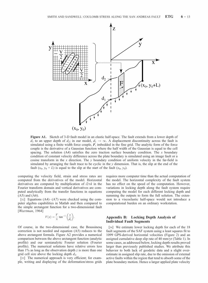
[40] We wish to calculate the displacement vectoru(x, y, z) due to a vector body force at depth. This approachis used to describe motion on both curved and discontinuousfaults, and is also used to evaluate stress regimes above theupper locking depth. For simplicity, we ignore the effects ofEarth’s sphericity. We assume a Poisson material, andmaintain constant moduli with depth. A major differencebetween this solution and the Okada [1985, 1992] solutionsis that we consider deformation due to a vector body force,while the Okada solution considers deformation due to adislocation.[41] While the following text provides a brief outline of

our model formulation, the full derivation and source codeof our semianalytic Fourier model can be found at http://topex.ucsd.edu/body_force. Our solution is obtained asfollows:[42] 1. Develop three differential equations relating a

3-D vector body force to a 3-D vector displacement. Weapply a simple force balance in a homogeneous, isotropicmedium and after a series of substitutions for stress, strain,and displacement, we arrive at equation A1, where u, v, andw are vector displacement components in x, y, and z, l and mare Lame parameters, rj are vector body force components:

mr2uþ lþ mð Þ @2u

@x2þ @2v

@ydxþ @2w

@z@x

� �¼ �rx

mr2vþ lþ mð Þ @2u

@x@yþ @2v

@y2þ @2w

@z@y

� �¼ �ry

mr2wþ lþ mð Þ @2u

@xdzþ @2v

@ydzþ @2w

@z2

� �¼ �rz

ðA1Þ

A vector body force is applied at x = y = 0, z = a. Topartially satisfy the boundary condition of zero sheartraction at the surface, an image source is also applied atx = y = 0, z = �a [Weertman, 1964]. Equation (A2)describes a point body force at both source and imagelocations, where F is a vector force with units of force:

R x; y; zð Þ ¼ Fd xð Þd yð Þd z� að Þ þ Fd xð Þd yð Þd zþ að Þ ðA2Þ

[43] 2. Take the 3-D Fourier transform of equations (A1)and (A2) to reduce the partial differential equations to a setof linear algebraic equations.[44] 3. Invert the linear system of equations to isolate the

3-D displacement vector solution for U(k), V(k), and W(k).

U kð Þ

V kð Þ

W kð Þ

266664

377775 ¼ lþ mð Þ

kj j4m lþ 2mð Þ

k2y þ k2z

� �þ m kj j2

lþ mð Þ �kykx �kzkx

�kxky k2x þ k2z� �

þ m kj j2

lþ mð Þ �kzky

�kxkz �kykz k2x þ k2y

� �þ m kj j2

lþ mð Þ

2666666664

3777777775

e�i2pkza þ ei2pkza� �

4p2

Fx

Fy

Fz

266664

377775 ðA3Þ

where k = (kx, ky, kz) and jkj2 = k . k.[45] 4. Perform the inverse Fourier transform in the z

direction (depth) by repeated application of the Cauchyresidue theorem. We assume z to be positive upward.[46] 5. Solve the Boussinesq problem to correct for non-

zero normal traction on the half-space. This derivationfollows the approach of Steketee [1958] where we imposea negative surface traction in an elastic half-space in order tocancel the nonzero traction from the source and image in theelastic full-space.[47] 6. Integrate the point source Green’s function to

simulate a fault. For a complex dipping fault, this integra-tion could be done numerically. However, if the faults areassumed to be vertical, the integration can be performedanalytically. The body force is applied between the lowerdepth d1 (e.g., minus infinity) and the upper depth d2(Figure A1). The displacement or stress (derivatives arecomputed analytically) can be evaluated at any depth zabove d2. Note that the full displacement solution is the sumof three terms: a source, an image, and a Boussinesqcorrection.

U kð Þ

V kð Þ

W kð Þ

266664

377775 ¼

Uxs Uys Uzs

Uys Vys Vzs

Uzs Vzs Wzs

266664

377775

Fx

Fy

Fz

266664

377775þ

Uxi Uyi �Uzi

Uyi Vyi �Vzi

Uzi Vzi �Wzi

266664

377775

Fx

Fy

Fz

266664

377775þ

UB

VB

WB

266664

377775 ðA4Þ


[48] The individual elements of the source and imagetensors are

Uxs kð Þ ¼ C

b2e�b z�d2ð Þ Dþ

k2y

kj j2� k2x

kj j21þ b z� d2ð Þð Þ

" #(

�e�b z�d1ð Þ Dþk2y

kj j2� k2x


" #)

Uys kð Þ ¼ � C

b2kxky

kj j2e�b z�d2ð Þ 2þ b z� d2ð Þð Þ

n

�e�b z�d1ð Þ 2þ b z� d1ð Þð Þo

Uzs kð Þ ¼ �iC

b2kx

kj j e�b z�d2ð Þ 1þ b z� d2ð Þð Þn


Vys kð Þ ¼ C

b2e�b z�d2ð Þ Dþ k2x

kj j2�

k2y


" #(

�e�b z�d1ð Þ Dþ k2x

kj j2�

k2y


" #)

Vzs kð Þ ¼ �iC

b2ky

kj j e�b z�d2ð Þ 1þ b z� d2ð Þð Þn


Wzs kð Þ ¼ C

b2e�b z�d2ð Þ Dþ 1þ b z� d2ð Þ½

n

�e�b z�d1ð Þ Dþ 1þ b z� d1ð Þ½ o

Uxi kð Þ ¼ C

b2eb zþd2ð Þ Dþ

k2y

kj j2� k2x

kj j21� b zþ d2ð Þð Þ

" #(

�eb zþd1ð Þ Dþk2y

kj j2� k2x


" #)

Uyi kð Þ ¼ � C

b2kxky

kj j2eb zþd2ð Þ 2� b zþ d2ð Þð Þ

n

�eb zþd1ð Þ 2� b zþ d1ð Þð Þo

Uzi kð Þ ¼ iC

b2kx

kj j eb zþd2ð Þ 1� b zþ d2ð Þð Þn


Vyi kð Þ ¼ C

b2eb zþd2ð Þ Dþ k2x

kj j2�

k2y


" #(

�eb zþd1ð Þ Dþ k2x

kj j2�

k2y


" #)

Vzi kð Þ ¼ iC

b2ky

kj j eb zþd2ð Þ 1� b zþ d2ð Þð Þn


Wzi kð Þ ¼ C

b2eb zþd2ð Þ Dþ 1� b zþ d2ð Þ½

n

�eb zþd1ð Þ Dþ 1� b zþ d1ð Þ½ o

where

C ¼ lþ mð Þ4m lþ 2mð Þ D ¼ lþ 3m

lþ ma ¼ lþ m

lþ 2m

kj j ¼ k2x þ k2y

� �1=2b ¼ 2p kj j:

[49] The individual elements of the Boussinesq correctionare

UB ¼ �i2pkx1

2mt3 kð Þb3

1� 1

a� bz

� �ebz

VB ¼ �i2pky1

2mt3 kð Þb3

1� 1

a� bz

� �ebz

WB ¼ � 1

2mt3 kð Þb2

1

a� bz

� �ebz

ðA6Þ

where

t3 ¼�ikx

kj j ebd2 abd2 �l

lþ 2mð Þ

� �� ebd1 abd1 �

llþ 2mð Þ

� ��Fx

�

�iky

kj j ebd2 abd2 �l

lþ 2mð Þ

� �� ebd1 abd1 �

llþ 2mð Þ

� ��Fy

�

þ ebd2 abd2 �m

lþ 2mð Þ � 2a� ��

�ebd1 abd1 �m

lþ 2mð Þ � 2a� ��

Fz: ðA7Þ

[50] 7. Construct a force couple by taking the derivativeof the point source in the direction normal to the fault trace.In practice, the body forces due to the stress discontinuityacross a fault plane are approximated by the derivative of aGaussian function, effectively producing a model fault witha finite thickness (Figure A1). Curved faults are constructedwith overlapping line segments having cosine tapered endsand are typically 6–10 km long.[51] The fault trace is imbedded in a two-dimensional grid

which is Fourier transformed, multiplied by the transferfunctions above, equations (A5)–(A7), and inverse Fouriertransformed. A constant shear modulus (4.12� 1010 Pa) andPoisson ratio (0.25) were adopted for all calculations. Whenthe lower edge of the fault is extended to infinite depth, as inthe case of the SAF systemmodel, a Fourier cosine transform(mirrored pair) is used in the across-fault direction to main-tain the far-field velocity V step across the plate boundary,effectively conserving moment within the grid. Note that thisrequires the velocity difference (i.e., stress drop) across asystem of connecting faults to have a constant value F = mV.To avoid Fourier artifacts where the fault enters the bottom ofthe grid and leaves the top of the grid, the fault is extendedbeyond the top of the model and angled to match theintersection point at the bottom (Figure A1). In addition to

(A5)


computing the velocity field, strain and stress rates arecomputed from the derivatives of the model. Horizontalderivatives are computed by multiplication of i2pk in theFourier transform domain and vertical derivatives are com-puted analytically from the transfer functions in equations(A5) and (A6).[52] Equations (A4)–(A7) were checked using the com-

puter algebra capabilities in Matlab and then compared tothe simple arctangent function for a two-dimensional fault[Weertman, 1964]

V xð Þ ¼ V

ptan�1 x

d2

� �:

Of course, in the two-dimensional case, the Boussinesqcorrection is not needed and equation (A5) reduces to theabove arctangent formula. Figure A2 provides a numericalcomparison between the above arctangent function (analyticprofile) and our semianalytic Fourier solution (Fourierprofile). The numerical solutions have relative errors lessthan 1% as long as the observation depth z is more than onegrid cell size above the locking depth d2.[53] The numerical approach is very efficient; for exam-

ple, writing and displaying of the deformation/stress grids

requires more computer time than the actual computation ofthe model. The horizontal complexity of the fault systemhas no effect on the speed of the computation. However,variations in locking depth along the fault system requirecomputing the model for each different locking depth andsumming the outputs to form the full solution. The exten-sion to a viscoelastic half-space would not introduce acomputational burden on an ordinary workstation.

Appendix B: Locking Depth Analysis ofIndividual Fault Segments

[54] We estimate lower locking depth for each of the 18fault segments of the SAF system using a least squares fit to1099 GPS-derived horizontal velocities (Figure 2) and anassigned cumulative deep slip rate of 40 mm/yr (Table 1). Insome cases, as addressed below, locking depth results provedlarger than previously published studies. We attribute thisbehavior to both lack of geodetic data and a slight over-estimate in assigned slip rate, due to the omission of externalactive faults within the region that tend to absorb some of theplate boundary motion. Hence a larger applied plate velocity

Figure A1. Sketch of 3-D fault model in an elastic half-space. The fault extends from a lower depth ofd1 to an upper depth of d2; in our model, d1 ! 1. A displacement discontinuity across the fault issimulated using a finite width force couple, F, imbedded in the fine grid. The analytic form of the forcecouple is the derivative of a Gaussian function where the half width of the Gaussian is equal to the cellspacing. The solution (A4) satisfies the zero traction surface boundary condition. The x boundarycondition of constant velocity difference across the plate boundary is simulated using an image fault or acosine transform in the x direction. The y boundary condition of uniform velocity in the far-field issimulated by arranging the fault trace to be cyclic in the y dimension. That is, the slip at the end of thefault (x0, y0 + L) is equal to the slip at the start of the fault (x0, y0).


is effectively compensated by deeper locking of SAF faultsegments. However, applying a deep slip rate other than40 mm/yr does not significantly improve the fit to the GPSdata, and yields inconsistent long-term slip rates for individ-ual fault segments [WGCEP, 1995, 1999]. The locking depthresults of our best fitting model are summarized below.

B1. Profile 1, Segment 1

[55] The Imperial fault, shown in Profile 1 of Figure 2b, isbest modeled by a locking depth of 5.9 ± 1.2 km. Publishedvalues of locking depth for the Imperial fault range from 8 to13 km [Archuleta, 1984; Genrich and Bock, 1997; Lyons etal., 2002], typically accompanying 45 mm/yr of slip withvariations of surface creep. Genrich and Bock [1997] arguefor a 9 km locking depth but also cite 5 km as a reasonableminimum. Seismicity locations are identified at depths of7.5 km ± 4.5 km [Richards-Dinger and Shearer, 2000],lending equal validity to our more shallow locking depthestimate.[56] The Imperial fault is known to exhibit fairly complex

slip behavior with associated creep and perhaps cannot beaccurately modeled as a single fault segment that is simply

locked at depth. Because we do not included the effects ofshallow creep into our analysis, it is possible that our modelis forced to shallower locking depths in order to satisfy datathat do reflect fault creep. Conversely, the improved SCECvelocities may actually reveal the nature of a more shal-lowly locked fault than that of previous published models ofthe Imperial fault based on earlier data. It is also possiblethat the Imperial segment has a significant dipping compo-nent, producing an asymmetric displacement [Lyons et al.,2002]. Our model neglects the case of dipping faults as weassume that all segments of the SAF system are verticalfault planes.

B2. Profile 2, Segments 2 and 4

[57] Profile 2 compares velocities of both the Brawleysegment and Borrego segment. Our inversion results in alocking depth estimate of 6.3 ± 1.3 km for the Brawleyregion. Johnson and Hadley [1976] identified hypocentraldepths of earthquake swarms in the 4–8 km range for thisregion, placing our solution within acceptable range. Sim-ilarly, Johnson et al. [1994] present a 5 km locking depthmodel for the Brawley region based on work by Bird andRosenstock [1984], Weldon and Sieh [1985], Rockwell et al.[1990], and Sieh and Williams [1990]. Data are fairly sparsein the Borrego region, as evident in Profile 2, and do notshow significant evidence for fault deformation, resulting ina locking depth of 2.0 ± 7.7 km. Our model produced ratherunstable results for this segment, often leaning toward 0 kmlocking depth. We attribute this behavior to not only lack ofdata, but also the fact that the fault trace of this region wasestimated by connecting the lower Anza segment with theupper Imperial fault trace. In this region, many small sub-parallel branches exist [Larsen et al., 1992] and we havemost likely oversimplified the fault geometry. Seismicity isnot particularly evident within 10 km of our estimated faulttrace, and is found primarily to the southwest and constrictedto the upper 10 km of the crust [Hill et al., 1991]. Johnson etal. [1994] show seismicity clustered heavily in the upper5 km of the crust for the southernmost portion of ourmodeled region. They also identify a 5 km shallow lockingdepth solution for this region from geodetic observations.


[58] Profile 3 displays the major region of the San Jacintoand Coachella-San Bernardino fault segments (Figure 1,segments 5 and 3, respectively). We find a locking depth of22.6 ± 1.7 km for the greater portion of the Coachella-SanBernardino segment, providing a good match to the 25 kmdepth chosen by Feigl et al. [1993]. The San Jacinto regionis best modeled at 13.1 km ± 2.3 km, corresponding withinlimits of uncertainty to the 10–11 km locking depthestimated by previous models [Sanders, 1990; Savage,1990; Li and Lim, 1988]. Seismicity is heavily confinedto 10–20 km depths for the San Jacinto region [Johnson etal., 1994], placing our modeled estimate of 13 km withinacceptable limits. A visual inspection of Profile 3 alsoreveals the anomalous velocities associated with regionaldeformation due to the Eastern California Shear Zone(ECSZ), located east of the San Bernardino-Coachella trace.Our modeling efforts do not account for the complexdeformation evident in this region [Dokka and Travis,1990; Sauber et al., 1986; Savage, 1990], nor do we include

Figure A2. Example model output with arctangentfunction comparison. (a) Map view of an infinitely longfault in the y dimension imbedded in a 1-km spaced grid.We have assigned an upper locking depth of 5 km (d2) to thefault plane and have extended the lower depth to infinity(d1). (b) Comparison between the analytic solution ofWeertman [1964] and a fault-perpendicular profile of oursemianalytic Fourier model. The two solutions are virtuallyindistinguishable and have relative errors less than 1%.


the left-lateral Pinto Mountain Fault into our analysis, alsoknown to contribute additional complications in this area.


[59] Profile 4 displays our modeled Mojave segment at26 ± 1.7 km depth. Similarly, Eberhart-Phillips et al.[1990] propose a 25 km locking depth for this region.Savage [1990] argues for a 30 km locking depth estimatefor this portion of the Transverse Ranges using an elasticplate model overlying a viscoelastic half-space, providing arealistic match to our simple elastic half-space model.Thatcher [1983] illustrated a similar comparison for thisregion, making the valid point that two physically differentmechanisms (elastic vs. viscoelastic half-space) produceindistinguishable surface deformation. Again, we note theevident unmodeled velocities to the east of the fault tracethat are related to complex deformation patterns of theECSZ.


[60] The Carrizo segment, located just north of the BigBend, is shown in Profile 5, modeled at 25.2 ± 2.6 km.This value agrees well with previously published models of25 km locking depth [Eberhart-Phillips et al., 1990]. Weagain note anomalous velocities to the east of this region,consistent with Eastern California Shear Zone deformation.


[61] The Cholame segment, located in Profile 6, ismodeled best by a locking depth of 12.7 ± 2.4 km.Similarly, Richards-Dinger and Shearer [2000] note seis-micity located down to 12.5 km for this segment. King et al.[1987] prefer a model with a deep slip rate of 33 mm/yr anda locking depth of 16 km for this region, but also discuss thepotential for locking between 14 and 18 km for constraineddeep slip of 36 mm/yr. Our estimate of 12.7 km ± 2.4 kmplaces our results within reasonable agreement, although weconstrain our deep slip at 40 mm/yr for this segment.Alternatively, Li and Lim [1988] explore shallow lockingdepths (4–9 km) as a plausible fit to the Cholame region.


[62] The Parkfield segment is shown in Profile 7, mod-eled at 14.5 ± 2.9 km locking depth. It should be noted thatthe Parkfield segment incorporates a transitioning region ofslip from a locked fault to that of aseismic creep [Harris andSegall, 1987]. Because this slip transition occurs along the25 km length of the fault segment, our model finds aminimized misfit relating to the deeper locked portion tothe south. Harris and Segall [1987] also report a 14 kmtransition depth for the locked portion of the Parkfieldsegment. Our model estimate and uncertainty lie slightlydeeper than the 8–10 km locking depth published by Kinget al. [1987] but within uncertainty limits of the lockingdepth estimate of Eaton et al. [1970] of 10–12 km fromaftershocks of the 1966 earthquake that occurred along thefault. Richards-Dinger and Shearer [2000] provide seis-micity depths ranging from 11.4 km ± 6.7 km.


[63] Profile 8 shows our result for the creeping section ofthe SAF, just north of the Parkfield segment. Our inversionprovides a locking depth of 1.3 km ± 0.2 km, which does

not imply continuous or quasi-continuous slip (fault creep)at the surface, as would be expected from geologic andgeodetic estimates [Savage and Burford, 1973; Thatcher,1979]. Data coverage is rather weak for this region, and it ispossible that the geodetic measurements used in our anal-ysis do not completely capture the true behavior of aseismicsurface creep.


[64] Profile 9 displays modeled segments of the SanAndreas (Santa Cruz and Peninsula) fault along with theSouthern and Central Calaveras fault. We find that a 9.3 km ±0.6 km locking depth for the San Andreas region satisfies thedata well, corresponding nicely to the 10 km estimate usedby Feigl et al. [1993], and within acceptable limits to theestimate of 12 km by Murray and Segall [2001]. TheCalaveras fault, located to the east of the San Andreas faulttrace, exhibits regions of aseismic slip as it branches off inthe northeastward direction from the creeping portion of themain San Andreas strand. This segment is known to have ahigh creep rate of 12–17 mm/yr [WGECP, 1996; Bakun,1999], matching its long-term slip rate. We find that alocking depth of 1.6 km is required to accurately modelthe geodetic data for this region. This estimate agrees withOppenheimer et al.’s [1988] estimate of 1–2 km based onaftershock solutions of the Morgan Hill event of 1984.


[65] Further north, the Calaveras fault branches into theSouthern Hayward fault to the west and the NorthernCalaveras-Concord faults to the east. Profile 10 illustratesthis behavior and also captures the Santa Cruz-Peninsulasegment of the San Andreas as discussed above. We find alocking depth of 13.7 ± 4.6 km for the Northern Calaveras-Concord and 15.7 km ± 3.7 km for the Hayward region.While our model finds satisfactory locking depth estimatesfor this region, our results are rather unstable in that theytend to dramatically over and under estimate regions of thenorthern SAF system if left unbounded. The results wepresent here are most likely an unfortunate product of sparsedata for this region, as illustrated by their associateduncertainties. Attempts to constrain either of these segmentsto a more shallow depth (e.g., 10.4 km [Murray and Segall,2001] for Northern Calaveras-Concord or 12–14 km [Burg-mann et al., 2000; Simpson et al., 2001] for SouthernHayward) simply result in unacceptably deep locking depthresults for the remaining segments. Additions to the data setfor the northern SAF system will be required in order toplace better locking depth estimates for these regions.

B11. Profile 11, Segments 11, 17, and 14

[66] We obtain similar results for the segments incorpo-rated into Profile 11. Again, we model the Santa Cruz-Peninsula segment and Northern Calaveras-Concordsegment, now along with the Rodgers Creek segment. Weagain find a deeper locking depth than expected for theRodgers Creek segment at 18.9 km ± 6.7 km. This faultsegment is thought to be completely locked to the base ofthe seismogenic zone, exhibiting zero properties of shallowcreep [WGCEP, 1999]. Microseismicity suggests that thisfault segment extends to a depth of approximately 12 km[Budding et al., 1991], while hypocentral depths of two


1969 events of the Rodgers Creek fault were estimated at9.5 and 10.5 km depths [Steinbrugge et al., 1970]. Whileour model estimate of this fault is admittedly higher thansuch published depths, our regions of uncertainty are alsohigh, placing the modeled Rodgers Creek locking depthwithin acceptable limits. Again, additional data are neces-sary to make a better locking depth estimate of this segment.

B12. Profile 12, Segments 12, 15, and 18

[67] Finally, we present our results for the northernmostregion of the San Andreas system in Profile 12, modelingsegments of North Coast San Andreas, Maacama, andGreen Valley-Bartlett Springs faults. We find a 19.4 ±2.1 km locking depth best fits the North Coast section ofthe San Andreas Fault region, which agrees with Matthewsand Segall [1993], who propose a 15–20 km locking depth.Furlong et al. [1989] provide a valid explanation for suchdeep locking behavior, suggesting that the northern SanAndreas is connected to a deep shear zone by a subhor-izontal detachment at approximately 20 km depth. We alsofind locking depth values of 12.3 ± 4.3 km for the Maacamafault and 9.1 km ± 8.4 km for the Bartlett Springs fault.Unfortunately, seismicity depths are dispersed from 0 to15 km [Castillo and Ellsworth, 1993] for the eastern regionand do not help constrain our results. These three regionsare well modeled by Freymueller et al. [1999] with lockingdepth estimates of 14.9 km (+12.5/�7.1 km), 13.4 km(+7.4/�4.8 km), and 0 km (+5 km) for the North CoastSan Andreas, Maacama, and Green Valley-Barlett Springsfaults, respectively. While our estimates match those ofFreymueller et al. [1999] within their limits of uncertainty,we again note that the data coverage for this region isparticularly sparse and not extremely well posed for ourlocking depth inversion.

[68] Acknowledgments. We thank Duncan Agnew, Yehuda Bock,Jeff Freymueller, and Roland Burgman for providing the GPS velocitymeasurements and the guidance on how to use them. Yuri Fialko and DonnaBlackman provided careful in-house reviews of draft versions of themanuscript. We thank Ross Stein, Jim Savage, and the Associate Editor,Massimo Cocco, for their help on improving the manuscript and clarifyingthe model. This research was supported by the NASA Solid Earth andNatural Hazards program (NAGS-9623) and the NSF Earth ScienceProgram (EAR-0105896).

ReferencesArchuleta, R. J., A faulting model for the 1979 Imperial Valley earthquake,J. Geophys. Res., 89, 4559–4585, 1984.

Atwater, T., Plate tectonic history of southern California with emphasis onthe Western Transverse Ranges and Santa Rosa Island, in Contributionsto the Geology of the Northern Channel Islands, Southern California,edited by P. W. Weigand, pp. 1–8, Am. Assoc. of Pet. Geol., Pac. Sect.,Bakersfield, Calif., 1998.

Bakun, W., Seismic Activity of the San Francisco Bay Region, Bull. Seis-mol. Soc. Am., 89, 764–784, 1999.

Bird, P., and R. W. Rosenstock, Kinematics of present crust and mantleflow in southern California, Geo. Soc. Am. Bull., 95, 946–957, 1984.

Brown, R. D., Jr., Quaternary deformation, in The San Andreas FaultSystem California, edited by R. E. Wallace, U.S. Geol. Surv. Prof.Pap., 1515, 104–109, 1991.

Budding, K. E., D. P. Schwartz, and D. H. Oppenheimer, Slip rate, earth-quake recurrence, and seismogenic potential of the Rodgers Creek FaultZone, northern California: Initial results, Geophys. Res. Lett., 18, 447–450, 1991.

Burgmann, R., D. Schmidt, R. M. Nadeau, M. d’Alessio, E. Fielding,D. Manaker, T. V. McEvilly, and M. H. Murray, Earthquake potentialalong the northern Hayward fault, California, Science, 289, 1178–1182,2000.

Byerlee, J. D., Friction of rock, Pure Appl. Geophys., 116, 615–626, 1978.Castillo, D. A., and W. L. Ellsworth, Seismotectonics of the San Andreasfault system between Point Arena and Cape Mendocino in northern Ca-lifornia: Implications for the development and evolution of a young trans-form, J. Geophys. Res., 98, 6543–6560, 1993.

Chinnery, M. A., The deformation of the ground around surface faults, Bull.Seismol. Soc. Am., 51, 355–372, 1961.

Chinnery, M. A., The stress changes that accompany strike-slip faulting,Bull. Seismol. Soc. Am., 53, 921–932, 1963.

Craymer, M. R., and P. Vanicek, Comment on ‘‘Saugus-Palmdale, Califor-nia, field test for refraction error in historical leveling surveys’’ by R. S.Stein, C. T. Whalen, S. R. Holdahl, W. E. Strange, and W. Thatcher,and reply to ‘‘Comment on ‘Futher analysis of the 1981 Southern Cali-fornia field test for leveling refraction by M. R. Craymer and P. Vanicek’by R. S. Stein, C. T. Whalen, S. R. Holdahl, W. E. Strange, andW. Thatcher’’, J. Geophys. Res., 94, 7667–7672, 1989.

DeMets, C., R. G. Gordon, D. F. Argus, and S. Stein, Current plate motions,Geophys. J. Int., 101, 425–478, 1990.

DeMets, C., R. G. Gordon, D. F. Argus, and S. Stein, Effect of recentrevisions to the geomagnetic reversal time scale on estimates of currentplate motions, Geophys. Res. Lett., 21, 2191–2194, 1994.

Dokka, R. K., and C. J. Travis, Role of the Eastern California Shear Zone inaccommodating Pacific-North American plate motion, Geophys. Res.Lett., 17, 1323–1326, 1990.

Eaton, J. P., M. E. O’Neill, and J. N. Murdock, Aftershocks of the 1966Parkfield-Cholame, California earthquake: A detailed study, Bull. Seis-mol. Soc. Am., 60, 1151–1197, 1970.

Eberhart-Phillips, D., M. Lisowski, and M. D. Zoback, Crustal strain nearthe Big Bend of the San Andreas fault: Analysis of the Los Padres-Tehachapi trilateration networks, California, J. Geophys. Res., 95,1139–1153, 1990.

Elders, W. A., R. W. Rex, T. Meidav, P. T. Robinson, and S. Biehler, Crustalspreading in Southern California, Science, 178, 15–24, 1972.

Ellsworth, W. L., Earthquake history, 1769–1989, in The San AndreasFault System, California, edited by R. E. Wallace, U.S. Geol. Surv. Prof.Pap., 1515, 152–187, 1990.

Feigl, K. L., et al., Space geodetic measurements of crustal deformation incentral and southern California, 1984–1992, J. Geophys. Res., 98,21,677–21,712, 1993.

Fialko, Y., and M. Simons, Deformation and seismicity in the Coso geother-mal area, Inyo County, California: Observations and modeling usingsatellite radar interferometry, J. Geophys. Res., 105, 21,781–21,794,2000.

Freymueller, J. T., M. H. Murray, P. Segall, and D. Castillo, Kinematicsof the Pacific-North America plate boundary zone, northern California,J. Geophys. Res., 104, 7419–7441, 1999.

Furlong, K. P., W. D. Hugo, and G. Zandt, Geometry and evolution of theSan Andreas Fault Zone in northern California, J. Geophys. Res., 94,3100–3110, 1989.

Genrich, J. F., and Y. Bock, Crustal deformation across the Imperial Fault:Results from kinematic GPS surveys and trilateration of a densely spaced,small-aperture network, J. Geophys. Res., 102, 4985–5004, 1997.

Harris, R. A., and P. Segall, Detection of a locked zone at depth on theParkfield, California, segment on the San Andreas Fault, J. Geophys.Res., 92, 7945–7962, 1987.

Harris, R., and R. Simpson, Changes in static stress on southern Californiafaults after the 1992 Landers earthquake, Nature, 360, 251–254, 1992.

Hill, D. P., P. Mowinckel, and L. G. Peake, Earthquakes, active faults, andgeothermal areas in the Imperial Valley, California, Science, 188, 1306–1308, 1975.

Hill, D. P., J. P. Eaton, and L. M. Jones, Seismicity, 1980–1986, in The SanAndreas Fault System, California, edited by R. E. Wallace, U.S. Geol.Surv. Prof. Pap., 1515, 133–136, 1991.

Hudnut, K. W., L. Seeber, and J. Pacheco, Cross-fault triggering in theNovember 1987 Superstition Hills earthquake sequence, southern Cali-fornia, Geophys. Res. Lett., 16, 199–202, 1989.

Jennings, C. W., Fault activity map of California and adjacent areas withlocations and ages of recent volcanic eruptions, Data Map Ser. 6, 92 pp.,2 plates, map scale 1:750,000, Calif. Div. of Mines and Geol., Sacramen-to, 1994.

Johnson, C. E., and D. M. Hadley, Tectonic implications of the Brawleyearthquake swarm, Imperial Valley, California, January 1975, Bull. Seis-mol. Soc. Am., 66, 1133–1144, 1976.

Johnson, H. O., D. C. Agnew, and F. K. Wyatt, Present-day crustal defor-mation in southern California, J. Geophys. Res., 99, 23,951–23,974,1994.

Jones, L. M., Focal mechanisms and the state of stress on the San AndreasFault in southern California, J. Geophys. Res., 93, 8869–8891, 1988.

King, G. C. P., and M. Cocco, Fault interaction by elastic stress changes:New clues from earthquake sequences, Adv. Geophys., 44, 1–38, 2001.


King, G. C. P., R. S. Stein, and J. Lin, Static stress changes and thetriggering of earthquakes, Bull. Seismol. Soc. Am., 84, 935–953, 1994.

King, N. E., P. Segall, and W. Prescott, Geodetic measurements near Park-field, California, 1959–1984, J. Geophys. Res., 92, 2747–2766, 1987.

Lachenbruch, A. H., and J. H. Sass, The stress heat-flow paradox andthermal results from Cajon Pass, Geophys. Res. Lett., 15, 981–984, 1988.

Larsen, S. C., and R. S. Reilinger, Age constraints for the present faultconfiguration in the Imperial Valley, California: Evidence for northwest-ward propagation of the Gulf of California rift system, J. Geophys. Res.,96, 10,339–10,346, 1991.

Larsen, S., R. Reilnger, H. Neubegauer, and W. Strange, Global positioningsystem measurements of deformations associated with the 1987 Super-stition Hills earthquake: Evidence of conjugate faulting, J. Geophys. Res.,97, 4885–4902, 1992.

Li, V. C., and H. S. Lim, Modeling surface deformations at complex strike-slip plate boundaries, J. Geophys. Res., 93, 7943–7954, 1988.

Lisowski, M., J. C. Savage, and W. H. Prescott, The Velocity field along theSan Andreas Fault in central and southern California, J. Geophys. Res.,96, 8369–8389, 1991.

Lomnitz, C., F. Mooser, C. R. Allen, J. N. Brune, and W. Thatcher, Seis-micity and tectonics of the northern gulf of California region, Mexico-Preliminary results, Geophys. Int., 10, 37–48, 1970.

Lyons, S. N., Y. Bock, and D. T. Sandwell, Creep along the Imperial Fault,southern California, from GPS measurements, J. Geophys. Res.,107(B10), 2249, doi:10.1029/2001JB000763, 2002.

Matthews, M. V., and P. Segall, Estimation of depth-dependent fault slipfrom measured surface deformation with application to the 1906 earth-quake, J. Geophys. Res., 98, 12,153–12,163, 1993.

Minster, J. B., and T. H. Jordan, Vector constraints on western U.S. defor-mations from space geodesy neotectonics and plate motions, J. Geophys.Res., 92, 4798–4804, 1987.

Murray, M. H., and P. Segall, Modeling broadscale deformation in northernCalifornia and Nevada from plate motions and elastic strain accumula-tion, Geophys. Res. Lett., 28, 3215–4318, 2001.

Okada, Y., Surface deformation due to shear and tensile faults in a half-space, Bull. Seismol. Soc. Am., 75, 1135–1154, 1985.

Okada, Y., Internal deformation due to shear and tensile faults in a half-space, Bull. Seismol. Soc. Am., 82, 1018–1040, 1992.

Oppenheimer, D. H., P. A. Reasenberg, and R. W. Simpson, Fault planesolutions of the 1984 Morgan Hill, California, earthquake sequence:Evidence for the state of stress on the Calaveras Fault, J. Geophys.Res., 93, 9007–9026, 1988.

Parker, R. L., Nonlinear problems, in Geophysical Inverse Theory, pp.293–368, Princeton Univ. Press, Princeton, N. J., 1994.

Peterson, M., W. Bryant, C. Cramer, T. Cao, M. Reichle, A. Frankel,J. Lienkaemper, P. McCrory, and D. Schwartz, Probabilistic seismichazard assessment for the state of California, U.S. Geol. Surv. OpenFile Rep., 96-706, 1–64, 1996.

Pollitz, F. F., C. Wicks, and W. Thatcher, Mantle flow beneath a continentalstrike-slip fault: Postseismic deformation after the 1999 Hector Mineearthquake, Science, 293, 1814–1818, 2001.

Richards-Dinger, K. B., and P. M. Shearer, Earthquake locations in southernCalifornia obtained using source-specific station terms, J. Geophys. Res.,105, 10,939–10,960, 2000.

Rockwell, T., C. Loughman, and P. Merifield, Late Quaternary rate of slipalong the San Jacinto fault zone near Anza, southern California, J. Geo-phys. Res., 95, 8593–8605, 1990.

Rybicki, K., Analysis of aftershocks on the basis of dislocation theory,Phys. Earth Planet Inter., 7, 409–422, 1973.

Sanders, C. O., Earthquake depths and the relation to strain accumulationand stress near strike-slip faults in southern California, J. Geophys. Res.,95, 4751–4762, 1990.

Sauber, J., W. Thatcher, and S. C. Solomon, Geodetic measurements ofdeformation in the central Mojave Desert, California, J. Geophys. Res.,91, 12,683–12,693, 1986.

Savage, J. C., Equivalent strike-slip earthquake cycles in half-space andlithosphere-asthenosphere earth models, J. Geophys. Res., 95, 4873–4879, 1990.

Savage, J. C., and R. O. Burford, Geodetic determination of relative platemotion in central California, J. Geophys. Res., 78, 832–845, 1973.

Savage, J. C., and M. Lisowski, Inferred depth of creep on the Haywardfault, central California, J. Geophys. Res., 98, 787–793, 1993.

Savage, J. C., and R. W. Simpson, Surface strain accumulation and theseismic moment tensor, Bull. Seismol. Soc. Am., 87, 1345–1353, 1997.

Savage, J. C., W. H. Prescott, M. Lisowski, and N. King, Deformationacross the Salton Trough, California, 1973–1977, J. Geophys. Res., 84,3069–3079, 1979.

Sieh, K. E., and P. L. Williams, Behavior of the southernmost San AndreasFault during the past 300 years, J. Geophys. Res., 95, 6629–6645, 1990.

Simpson, R. W., and P. A. Reasenberg, Earthquake-induced static stresschanges on central California faults, U.S. Geol. Surv. Prof. Pap., Rep. P1550-F, F55–F89, 1994.

Simpson, R. W., J. J. Lienkaemaper, and J. S. Galehouse, Variations increep rate along the Hayward Fault, California, interpreted as changesin depth of creep, Geophys. Res. Lett., 28, 2269–2271, 2001.

Stein, R. S., Contemporary plate motion and crustal deformation, Rev.Geophys., 25, 855–863, 1987.

Stein, R. S., and M. Lisowski, The 1979 Homestead Valley earthquakesequence, California: Control of aftershocks and postseismic deforma-tion, J. Geophys. Res., 88, 6477–6490, 1983.

Stein, R. S., G. C. P. King, and J. Lin, Stress triggering of the 1994M = 6. 7Northridge, California, earthquake by its predecessors, Science, 265,1432–1435, 1994.

Steinbrugge, K. V., W. K. Cloud, and N. H. Scott, The Santa Rosa, Cali-fornia, earthquakes on October 1, 1969, vol. 1970, pp. 1–63, U.S. En-viron. Sci. Serv. Admin., Silver Spring, Md., 1970.

Steketee, J. A., On Volterra’s dislocations in a semi-infinite elastic medium,Can. J. Phys., 36, 192–205, 1958.

Thatcher, W., Systematic inversion of geodetic data in central California,J. Geophys. Res., 84, 2283–2295, 1979.

Thatcher, W., Nonlinear strain buildup and the earthquake cycle on the SanAndreas Fault, J. Geophys. Res., 88, 5893–5902, 1983.

Ward, S. N., Pacific-North America plate motions: New results from verylong baseline interferometry, J. Geophys. Res., 95, 21,965–21,981, 1990.

Ward, S. N., A multidisciplinary approach to seismic hazard in southernCalifornia, Bull. Seismol. Soc. Am., 84, 1293–1309, 1994.

Wdowinski, S., Y. Sudman, and Y. Bock, Geodetic detection of active faultsin S. California, Geophys. Res. Lett., 28, 2321–2324, 2001.

Weldon, R. J., II, and K. E. Sieh, Holocene rate of slip and tentativerecurrence interval for large earthquakes on the San Andreas Fault, CajonPass, southern California, Bull. Seismol. Soc. Am., 96, 793–812, 1985.

Weertman, J., Continuum distribution of dislocations on faults with finitefriction, Bull. Seismol. Soc. Am., 54, 1035–1058, 1964.

Williams, C. A., and R. M. Richardson, A rheologically layered three-dimensional model of the San Andreas Fault in central and southernCalifornia, J. Geophys. Res., 96, 16,597–16,623, 1991.

Working Group on California Earthquake Probabilities (WGCEP), Seismichazards in southern California: Probable earthquakes, 1994 to 2024, Bull.Seismol. Soc. Am., 85, 379–439, 1995.

Working Group on California Earthquake Probabilities (WGCEP), Earth-quake probabilities in the San Francisco Bay Region: 2000 to 2030–Asummary of Ffindings, U.S. Geol. Surv. Open File Rep. [Online], 99-517,version 1. 0, 1999.

Working Group on Northern California Earthquake Potential (WGNCEP),Database of potential sources for earthquakes larger than magnitude 6 innorthern California, U.S. Geol. Surv. Open File Rep., 96–705, 1996.

Yule, D., and K. Sieh, Neotectonic and paleoseismic investigation of theSan Andreas fault system, San Gorgonio Pass, 1996 SCEC Annu. Rep.14-08-001-A0899 C, pp. 70–74, South. Calif. Earthquake Cent., Los An-geles, Calif., 1997.

Zeng, Y., Viscoelastic stress-triggering of the 1999 Hector Mine earthquakeby the 1992 Landers earthquake, Geophys. Res. Lett., 28, 3007–3010,2001.

��D. Sandwell and B. Smith, Institute for Geophysics and Planetary

Physics, Scripps Institution of Oceanography, 9500 Gilman Drive, MailCode 0255, La Jolla, CA 92093-0225, USA. ([email protected];[email protected])


coulomb stress accumulation along the san andreas · pdf filecoulomb stress accumulation along...

Documents