count data time series models for telecommunications data

Kandidatuppsats i matematisk statistikBachelor Thesis in Mathematical Statistics

Count data time series models fortelecommunications dataBálint Fatér

Matematiska institutionen

Kandidatuppsats 2015:31Matematisk statistikDecember 2015

www.math.su.se

Matematisk statistikMatematiska institutionenStockholms universitet106 91 Stockholm

Mathematical StatisticsStockholm UniversityBachelor Thesis 2015:31

http://www.math.su.se

Count data time series models for

telecommunications data

Balint Fater∗

December 2015

Abstract

The aim of the thesis is to try out the Poisson time series model for

count data, in order to analyze telecommunications monitoring data

from Ericsson AB. The amount of data a telecommunications network

produces is untenable to check manually, and thus the detections of

malfunctions can be both time consuming and extremely lengthy.

In this thesis we will explore the implementation of the above men-

tioned count data time series model on a subset of the data from a

telecommunications network and the viability of such an approach, in

particular, we will using identity link based generalized linear models

to perform the analysis- We will also attempt to select the best model

amongst several based on Akaike’s information criteria. Finally we

will cover how to implement said models in R and cover some of the

more technical aspects of the Poisson time series model for count data.

It turns out that the model fits quite well on most of the studied

time series, although, some of the data the telecommunications net-

work produces have counts in order of magnitudes of millions, hence

a better approach would probably have been to use an ordinary time

series based framework using a Gaussian response model.

∗Postal address: Mathematical Statistics, Stockholm University, SE-106 91, Sweden.

E-mail: [email protected]. Supervisor: Michael Hohle.

Acknowledgements

I would like to thank my supervisor, Michael Hohle, for the massive supportand help I received with this project. His kind and some times not so kindfeedback was a great help in improving the quality of this thesis, as wellas, helping me staying on track. Paolo Elena and Jan Petterson both atEricsson AB provided me with the data and readily answered any and allquestions I might have had. Last but not least I would like to thank StenMogren for always making sure I had access to everything I needed wheneverI was working at Ericsson. My most sincere thank you to you all.

Balint FaterStockholm, November 2015

2

Contents

1 Introduction 41.1 Aim of Thesis . . . . . . . . . . . . . . . . . . . . . . . . . . . 41.2 Overview of a telecommunications network . . . . . . . . . . 4

1.2.1 RNC - Radio Network Controller . . . . . . . . . . . . 41.2.2 RBS - Radio Base Station . . . . . . . . . . . . . . . . 5

2 Data Description 62.1 Counter 1 - A counter for number of load sharing diversions

caused by high load when connecting to the network . . . . . 62.2 Counter 2 - A counter for number of dropped calls . . . . . . 102.3 Counter 3 - A counter for number of occurances when lacking

rescources due to high load on the network . . . . . . . . . . 122.4 Counter 4 - A counter for the sum of all CS64 rescources

added to an existing call . . . . . . . . . . . . . . . . . . . . . 142.5 Summary . . . . . . . . . . . . . . . . . . . . . . . . . . . . . 16

3 Short introduction to generalized linear models 173.1 Parameter estimation . . . . . . . . . . . . . . . . . . . . . . 183.2 Model Validation . . . . . . . . . . . . . . . . . . . . . . . . . 193.3 Model Selection . . . . . . . . . . . . . . . . . . . . . . . . . . 19

4 Implementation on telecom data 204.1 Improving on model 4 for counter 2 . . . . . . . . . . . . . . . 23

5 Conclusion 30

References 31

3

1 Introduction

1.1 Aim of Thesis

In this thesis we will explore implementing the Poisson time series model forcount data on time series count data provided by Ericsson. The data origi-nated from one of their telecommunication networks, the location cannot bedisclosed due to a non disclosure agreement governing the data, however thelocation is not important for the present analysis. In order to provide thenecessary background knowledge, we will in this chapter, give a rudimentaryoverview of how a telecommunication network functions. In chapter two wewill cover the data in detail while in chapter three go over the technicaldetails of said Poisson time series model for count data, as well as somebackground calculations. I chapter four we will take look at how to imple-ment said model into R as well as select the most suitable individual modelfrom a set of possible candidates.

1.2 Overview of a telecommunications network

In a somewhat simplified model of a telecommunications network or ra-dio access network (RAN) consist of one or more radio network controllers(RNC) that each handles one or more radio base stations (RBS), which inturn handles multiple cells which are geographical areas. For instance theold city center of Stockholm “Gamla stan”, might in theory be handled byone RBS with four cells each spanning a quadrant as illustrated in Figure1. In reality Gamla stan is divided into many more cells, one reason be-ing the high roofs. There are also probably multiple networks covering thearea, since I am assuming that some Swedish phone operators use separatenetworks.

1.2.1 RNC - Radio Network Controller

The RNC is the node that controls all RAN functions. There are two distinctroles for the RNC, to serve and to control. The Serving RNC has overallcontrol of the phone that is connected to the RAN. It controls key andfrequently used resources, such as different voice bands, internet etc. TheControlling RNC has the overall control of a particular set of cells, and theirassociated base stations. When a phone must use resources in a cell notcontrolled by its Serving RNC, the Serving RNC must ask the ControllingRNC for those resources. An RNC is in contact with both other RNCs andwith all RBS under its control.

4

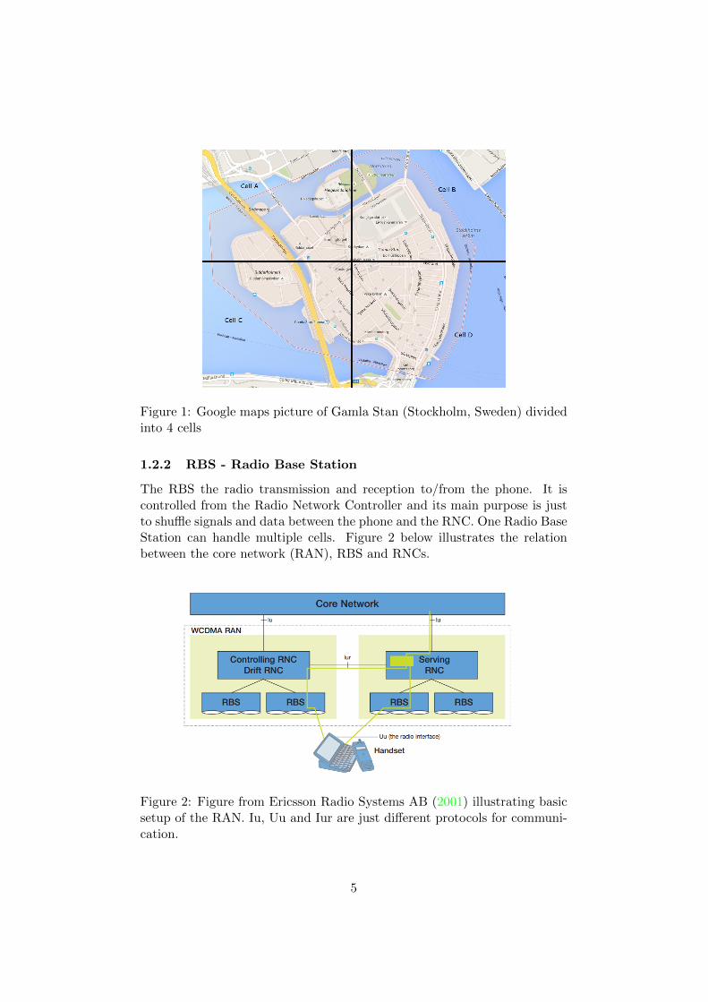
Figure 1: Google maps picture of Gamla Stan (Stockholm, Sweden) dividedinto 4 cells

1.2.2 RBS - Radio Base Station

The RBS the radio transmission and reception to/from the phone. It iscontrolled from the Radio Network Controller and its main purpose is justto shuffle signals and data between the phone and the RNC. One Radio BaseStation can handle multiple cells. Figure 2 below illustrates the relationbetween the core network (RAN), RBS and RNCs.

Figure 2: Figure from Ericsson Radio Systems AB (2001) illustrating basicsetup of the RAN. Iu, Uu and Iur are just different protocols for communi-cation.

5

2 Data Description

The data we received from Ericsson is 3 months of counter data from a fullsized RAN, its location cannot be disclosed due to a confidentiality agree-ment with Ericsson. There are many events in such a network that needsto be tracked for maintenance and anomaly detection purposes. The wayit is done here, there are counters for a set of predetermined events thatcount the amount of occurrences within a limited time frame. For instance,if someone were to call from this network first the counter for access wouldcount up one, then the counter for attempts would count up one and soforth. The same way if your call would be suddenly disconnected then thecounter for unexpected termination as well as the counter for drops fromthe network would increase by one.

Our data is divided into 15 minute intervals which gives us 96 data pointsfor each counter each day. In total we have access to roughly 3 months worthof data, starting from 3rd of March 2015 up to 1st of June 2015, in total 8682data points. In the present thesis we are going to focus on 4 counters, thesehave been chosen based on discussions with Ericsson testers for being keyindicators for the health of the network as well as being within the suitablerange that count data time series are useful for.

2.1 Counter 1 - A counter for number of load sharing di-versions caused by high load when connecting to thenetwork

This counter is used to count the number of times the RNC has to askneighboring RNCs to take over some tasks due to high load. Lets take alook at the first three weeks (more would not make the resulting graph veryclear) of data and see if we can discern any patterns (figure 3).

We note that there seem to be a strong daily and weekly cycle in data,weekends seem to produce less load then weekdays (remember data startson a Tuesday). Lets take a look at some box plots to see if our suspicion iscorrect (Figure 4):

6

Mar 03 00:00 Mar 08 00:00 Mar 13 00:00 Mar 18 00:00 Mar 23 00:00

0500

1000

1500

2000

2500

3000

3500

First month of Counter 1

Num

ber

of occurr

ences

Figure 3: First 3 weeks of Counter 1

7

0

2000

4000

Monday Tuesday Wedensday Thursday Friday Saturday Sunday

Counte

r 1 (

Num

ber

of occurr

ences

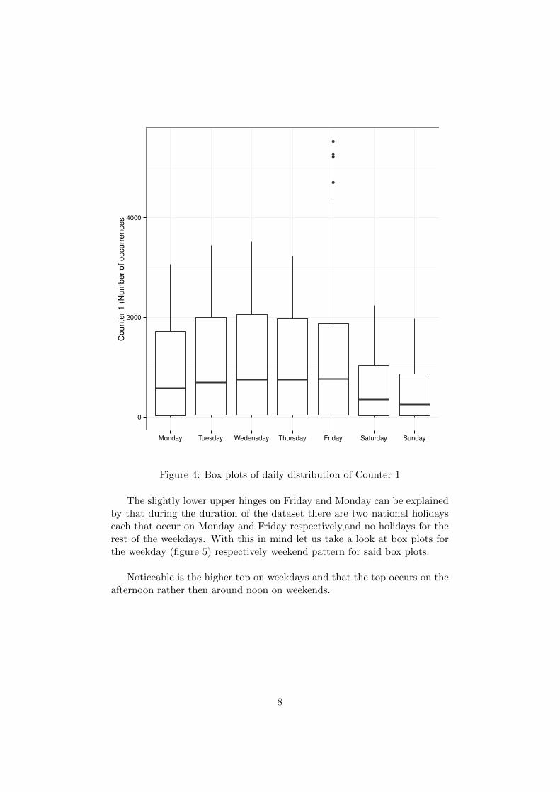
Figure 4: Box plots of daily distribution of Counter 1

The slightly lower upper hinges on Friday and Monday can be explainedby that during the duration of the dataset there are two national holidayseach that occur on Monday and Friday respectively,and no holidays for therest of the weekdays. With this in mind let us take a look at box plots forthe weekday (figure 5) respectively weekend pattern for said box plots.

Noticeable is the higher top on weekdays and that the top occurs on theafternoon rather then around noon on weekends.

8

●

●

●●●●●●

●●●●●●●●●

●●●●●●●●

●

●●●●●●●●

●●●●●●●●●●●●●●●●●●●●●●●●●●●

●

●●●●●●●

●

●● ●●●●●●●

●●●●●●●●

●●●●●●

●

●●●

●●

●

●

●

●

●●

●

●

●

●

●

●

●

●

●

●

●●

●

●

●●

●●

●

●

●

●

●

●

●

●

●●●

●

●

●●

●

●

●

●

●

●●

●

●

●●

●●

●

●

●●

●

●

●

●●

●●

●

●

●●

●●

●

●

●

●

●

●●

●

●

●

●

●

●

●

●

●

●

●

●

●

●

●

●

●

●

●

●

●●

●

●

●

●

●

●

●

●

●●●●

●

●

●

●

●

●

●●●

●

●

●

●

●●

●

●

●

●

●●

●

●●

●

●

●

●

●

●

●

●

●

●

●

●

●

●

●●

●

●

●

●

●

●

●●

●

●

●●

●

●

●

●

●

●

●

●

●●

●●●

●●

●

●

●

●

●

●

●

●

●

●

●

●

●●

●

●

●

●

●

●

●

●

●

●

●

●

●

●

●

●

●

●

●

●

●

●●

●●

●

●

●

●

●

●

●●

●

●●

●

●

●

●●

●

●

●

●

●

●

●

●

●●

●

●

●●

●

●

●

●●●

●

●

●●

●

●

●●●●●

●

●●

●

●

●

●

●●

●

●

●

●●

●●●●

●

●●

●

●

●●

●

●

●

●●●

●

●●●●●

●●

●●●

●

●

●

●

●

●

●

●

●

●

●

●●

●

●●

●

●

●

●

●●●

●●●●●●●

●●

●●

●●

●●●

●

●

●

●

●

●

●

●

●●

●

●

●●●●

●

●

●●●

●

●●●

●

●●●

●●

0

1000

2000

3000

4000

0100 0300 0500 0700 0900 1100 1300 1500 1700 1900 2100 2300Time of Day (hours)

Cou

nter

1 (

Num

ber

of o

ccur

renc

es)

Overview of daily cycle (weekdays)

●●

●●

●●

●●

●●

●

●

●●●●

● ●●●● ●●●●●●

●

●●

●●●●

●

●

●●●

●●●

●

●

●

●●

●

●

●

●

●

●

●●

●●

●

●●

●

●●

●

●

●

●

●

●●

●

●

●●●

●

●

●

●

●

●

●

●●●

●

●

●

●

●

●

● ●

●

●

●

●

●

●

●●

●

●●●● ●

●

●●●

●

●

●

● ●

●

●

●

●

●

●

●

●

●●

●

●

●

●●

●

●

●

●

●●

●

●●

●

●

●●

0

500

1000

1500

2000

0100 0300 0500 0700 0900 1100 1300 1500 1700 1900 2100 2300Time of Day (hours)

Cou

nter

1 (

Num

ber

of o

ccur

renc

es)

Overview of daily cycle (weekends)

Figure 5: Box plot of daily cycle for weekday respectively weekends

9

2.2 Counter 2 - A counter for number of dropped calls

There are a multitude of reasons dropped calls can occur in the RAN. Theseinclude bad coverage and lack of resources during a handover between net-works. Neither of which is desirable. Lets take a look at a box plot for thedaily distribution of data for counter 2 (figure 6):

0

50

100

150

200


Counte

r 2 (

Num

ber

of occurr

ences)


Similar to counter one we see that weekends have somewhat lower loadthen weekdays. Lets explore this in the plots below (figure 7):

Just as counter two we see very similar behavior between weekends andweekdays with the distinction being weekdays having consistently higherload then weekdends.

10

●

●●●●●

●

●●●●

●●

●

●

●

●●●●

●

●

●●●

●●●●●●●●●●●●●●●●●●●●●●

●●●●●●●●●

●●●●

●

●●

●

●●●

●

●●

●

●●

●

●

●

●

●

●

●

●

●

●

●

●

●

●

●

●

●

●

●

●●

●

●

●

●

●

●

●

●

●

●

●

●

●

●

●

●

●

●

●

●●

●

●

●

●

●

●●

●

●

●

●

●

●

●

●

●

●

●

●

●

●

●

●

●

●

●

●

●

●

●

●

●●

●

●

●

●

●

●

●

●

●

●

●

●

●

●

●

●

●●

●

●

●

●

●

●●●

●

●

●●

●

●

●

●

●

●

●

●●

●

●

●

●

●●

●

●

●

●

●

●

●

●

●

●

●

●

●

●

●

●

●

●

●

●

●

●●

●

●

●

●

●

●

●

●

●

●

●

●

●

●●

●

●

●●

●

●

●

●

●

●

●

●

●

●

●

●

●

●

●

●

●

●●

●

●

●

●

●●

●●

●

●

●

●

●

●

●

●

●●

●

●●

●

●

●

●

●

●

●

●●

●

●

●

●

●

●

●

●

0

50

100

150

0100 0300 0500 0700 0900 1100 1300 1500 1700 1900 2100 2300Time of Day (hours)

Cou

nter

2 (

Num

ber

of o

ccur

renc

es)


●●

●

●

●●

●

●●● ●

●●●

●

●●

●

●

●●

●

●

●

●

●

●

●●●

●

●

●●

●

●●

●

●●●

●

●

●●

●

●

●

●

●

●

●

●

●

●

●●

●

●

●

●

●

●

●

●

●

●

●

●

●

●

●

●

●

●●

●

●

●

●

●

●

●

●●

●

●●●

●

●

●●

●

0

20

40

60

0100 0300 0500 0700 0900 1100 1300 1500 1700 1900 2100 2300Time of Day (hours)

Cou

nter

2 (

Num

ber

of o

ccur

renc

es)



11

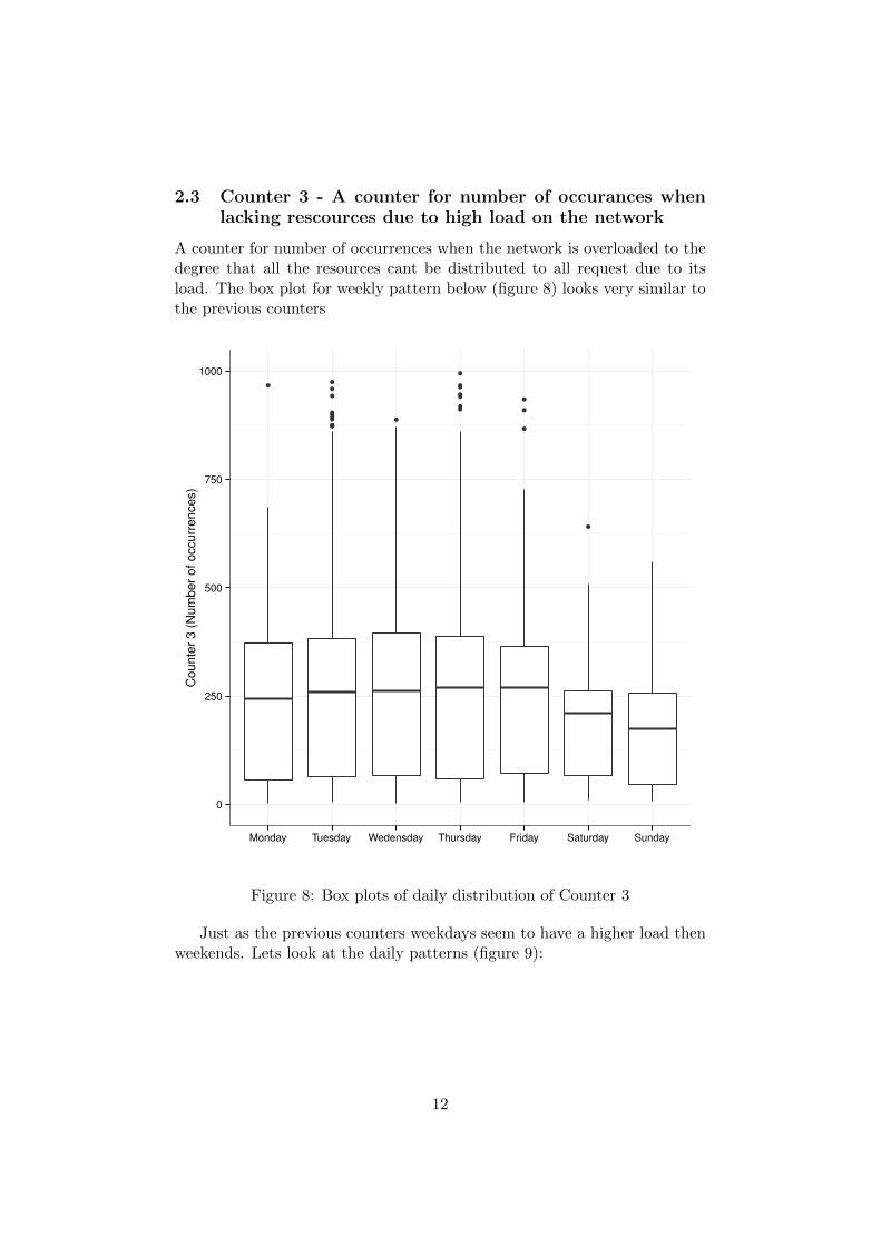
2.3 Counter 3 - A counter for number of occurances whenlacking rescources due to high load on the network

A counter for number of occurrences when the network is overloaded to thedegree that all the resources cant be distributed to all request due to itsload. The box plot for weekly pattern below (figure 8) looks very similar tothe previous counters

0

250

500

750

1000


Counte

r 3 (

Num

ber

of occurr

ences)


Just as the previous counters weekdays seem to have a higher load thenweekends. Lets look at the daily patterns (figure 9):

12

●

●

●●

●

●

●

●

●

●

●

●

●

●

●

●●

●●

●

●●

●●

●●

●

●

●

●

●

●

●

●

●

●

●

●

●

●

●

●

●

●

●

●

●

●

●●

●

●

●

●

●●

●

●

●

●

●

●●

●

●

●

●

●●

●

●

●

●●

●

●

●

●

●

● ●

●

●●

●

●

●

●

●

●

●

●

●

●●

●●

●

●

●

●

●

●

●

●

●

●

●

●

●

●

●●

●

●●

●

●

●

●

●●●

●

●

●

●

●●

●

●

●

●

●

●

●

●

●

●

●

●

●

●●

●

●

●●

●

●

●

●

●

●

●

●

●

●

●

●●

●●

●

●●

●

●

●

●●

0

200

400

600

800

0100 0300 0500 0700 0900 1100 1300 1500 1700 1900 2100 2300Time of Day (hours)

Cou

nter

3 (

Num

ber

of o

ccur

renc

es)


●

●

●

●

●●●●

●●●●

●

●

●●

●●

●●●●

●

●

●●

●

●

●

●

●●

●

●

●

●

●

●

●

●

● ●●

●

●

●

●●

●

●

●●●

●

●

●

●

●

●

●

●

●

●

●

●

●

●

●

●

●

0

200

400

600

0100 0300 0500 0700 0900 1100 1300 1500 1700 1900 2100 2300Time of Day (hours)

Cou

nter

3 (

Num

ber

of o

ccur

renc

es)



Again very similar to the previous 2 counters weekends have a consis-tently lower load then weekdays.

13

2.4 Counter 4 - A counter for the sum of all CS64 rescourcesadded to an existing call

Counter 4 is a counter that counts the amount of occurrences of CS64 re-source being added to an existing call. Resources are usually added to a callif during the call one starts video chat, starts to surf etc, CS64 is one suchresource. Here we see less of a weekly pattern with Mondays having similardensity to Saturdays (figure 10):

0

100

200

300

400

500


Counte

r 4 (

Num

ber

of occurr

ences)

Figure 10: Boxplots of daily distribution of Counter 4

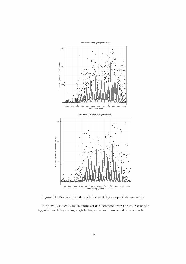
With this in mind lets explore the daily patterns for weekdays and week-ends and see if they differ from the previous counters (figure 11):

14

●

●

●

●

●●●●

●

●●●

●

●●●●●●●●●●●●●●●●●

●

●

●

●●●●

●

●●●●●●●●●●●●●●●●

●

●●

●

●●●●●●

●

●●●●●●●●●●●●●●●●●●●●●●●●

●●●●●●●●●●●

●

●

●

●

●

●●●●●●●●

●

●

●

●

●●●●●●●●●●

●

●●●●●●●

●

●●●●●

●

●●●●●●●●●●●

●

●

●

●●●●●

●

●●●

●

●

●

●

●●

●●

●●

●

●

●

●

●

●●

●

●

●

●

●

●

●●●

●●●

●

●

●

●

●

●

●

●

●

●●

●

●●

●

●

●

●

●

●

●

●

●

●

●●●

●

●

●

●●

●

●●●

●

●

●

●

●●●

●

●●

●

●

●●●

●

●

●

●

●

●

●

●

●

●

●

●

●●

●

●

●●

●

●●

●

●

●

●

●

●

●

●

●

●

●

●

●

●

●

●

●

●

●

●

●

●

●

●

●

●●

●

●

●

●

●

●

●

●●

●

●

●

●

●

●

●

●

●

●

●

●

●

●

●

●

●

●

●

●

●

●

●

●

●

●

●●

●

●

●

●●●

●

●●

●

●

●

●

●

●

●●

●●

●

●

●

●

●

●

●

●

●

●

●

●

●

●

●

●

●

●

●

●

●

●

●

●

●

●

●

●

●

●

●

●

●

●●

●

●

●

●

●

●

●

●

●

●

●●

●

●●

●●

●

●

●

●

●

●

●

●

●

●●

●

●

●

●

●

●

●

●

●

●

●

●

●

●

●

●

●●

●

●

●

●

●

●●

●

●

●

●

●

●

●

●

●

●

●

●

●

●

●

●

●

●

●

●

●

●

●

●●

●

●

●

●

●●

●

●●

●

●

●

●●

●

●

●

●

●

●

●

●

●

●

●

●

●

●

●

●

●●

●

●

●

●

●

●●●

●

●●

●

●

●

●

●

●

●

●

●

●

●

●

●

●

●

●

●

●

●

●

●

●

●

●

●

●

●

●

●

●●●

●

●

●

●

●

●

●

●

●

●

●

●

●

●

●

●

●

●

●

●

●

●

●●●●

●

●

●

●

●

●

●

●

●

●

●

●

●

●

●

●

●

●

●

●

●

●

●

●

●

●

●●●

●

●●●

●

●

●

●

●●

●

●

●

●

●

●

●●●

●

●

0

100

200

300

0100 0300 0500 0700 0900 1100 1300 1500 1700 1900 2100 2300Time of Day (hours)

Cou

nter

4 (

Num

ber

of o

ccur

renc

es)


●

●●●

●

●

●

●●

●

●●●●●●●●

●

●

●

●●●

●●●●

●

●●

●

●●

●

●

●

●●●●●

●

●●●●●●●●●●

●●●●

●

●

●

●

●

●

●

●

●

●

●

●

●●

●●●

●

●

●

●

●

●

●●

●

●●

●

●

●

●

●

●

●

●

●

●

●

●

●

●

●

●

●

●

●●

●

●

●

●

●

●

●

●

●

●

●

●

●

●

●

●

●

●

●

●

●

●

●

●

●

●

●●

●

●

●

●

●

●

●

●

●

●

●

●

●●●

●

●

●

●

●

●●

●

●

●

●

●

●

●

●

●

●

●

●

●

●

●

●

●

●

●

●

●

●

●

●

●

●

●

●

●

●

●

●

●

●

●

●

●

●

●

●

●

●

●

●

●

●

●

●

●

●●

●

●

●

●

●

●

●

●

●

●

●

●

●

●

●

●

●

●

●

●●

●

●

●●

●

●

●

●

●

●

●

●

●

●

●

●

●

●

●

●

●●

●

●●●●

●

●●●●

●

0

100

200

300

0100 0300 0500 0700 0900 1100 1300 1500 1700 1900 2100 2300Time of Day (hours)

Cou

nter

4 (

Num

ber

of o

ccur

renc

es)


Figure 11: Boxplot of daily cycle for weekday resepectivly weekends

Here we also see a much more erratic behavior over the course of theday, with weekdays being slightly higher in load compared to weekends.

15

2.5 Summary

One thing that is clear from the previous descriptive analysis is that all fourof our studied counters have a very strong daily and weekly cycles. Thedaily cycle is 24 hours and hence 96 observations long. Its noteworthy thatactivity during nightly hours are much lower across all 4 counters. Theweekly cycle is 674 data points long and here we note that weekends tendto have a lower ”top” then weekdays. In addition we can note that nationalholidays very similar to weekends. Counter 4 is somewhat a special case,while the patterns from the first three counters are present, the differencesare much more minute, with the daily pattern being much less clear as well.

Now that we are more familiar with the behavior of the data lets moveon to the theory behind the model we are going to implement.

16

3 Short introduction to generalized linear models

In this section we will take a look at the generalized linear model, moreprecisely the Poisson response model for time series that we will be using inthis thesis. We will also look at parameter estimation and model selectionfor this type of models.

Consider a nonnegative integer valued time series {Yt} called the responsetime series of said process. Furthermore let Ft−1 denote all available infor-mation on the process up to time t, this could also include covariates thatare known at time t, in our case, current date and time are two examples.According to Kedem and Fokianos (2002, p. 140) a most natural candidatedistribution for the response process is the Poisson. Then the conditionaldistribution of {Yt} is specified by assuming that the conditional density ofthe response given the past is Poisson with mean µt.

f(yt;µt|Ft−1) =exp(−µt)µytt

yt!, t = 1, ..., N. (1)

Furthermore we will define Zt−1, t = 1, ..., N as a p- dimensional covari-ate vector that includes past values of the response up to time t − 1 andpossibly any other supplementary information available up to time t.

In order to model the process {Yt} we will use a generalized linear model,which is an extension of the general linear model:

yt = xtβ + εt. (2)

The differences being the relaxation of the assumption that y is inde-pendently normally distributed with constant variance, instead the gener-alized linear model permits any distribution of the response that belongsto the exponential family, in our case the Poisson, and instead of modelingµt = E[yt|xt] directly as a function of the linear predictor ηt = xtβ, wemodel some function g(µt) of µt. Thus, the generalized linear model takesthe form

g(µt) = ηt = xtβ, (3)

with g(·) being called the link function. With the above in mind ourmodel then becomes, using the inverse link function h(·) = g−1(·), abovementioned covariate vector Zt−1 and the p-dimensional parameter vector forthe model β:

µt = h(Zt−1β), t = 1, ..., N. (4)

We will however concern ourselves with a Poisson model with identitylink, since it fits the aggregated nature of our data very well and the fact that

17

the traditional link function being a log link have the unfortunate tendencythat for unbounded covariates the proccess tends to grow at an exponatialrate (for more details see Kedem and Fokianos (2002, p. 143)). In this caseg(µt) = µt and as a consequence h(Zt−1β) = Zt−1β.

3.1 Parameter estimation

Now that we have formulated our time series Poisson model, we need toestimate the parameter vector β. The likelihood function is not alwayseasily obtainable, we will therefore use the partial likelihood function toestimate the β vector. Kedem and Fokianos (2002, p. 2) defines partiallikelihood as follows:

Definition 1 Denote the density of Yt, given the information Ft−1, byft(yt; θ) where θ ∈ Rp is a fixed parameter vector. The partial likelihood(PL) function relative to θ,Ft, and the data Y1, Y2, ..., YN , is given by theproduct

PL(θ; y1, y2, ..., yN ) =N∏t=1

ft(yt; θ). (5)

Conditional likelihood takes only into account what is known to theobserver up to time t. The partial likelihood function of β for the Poissonmodel is given by

PL(β) =N∏t=1

f(yt;β|Ft−1) =N∏t=1

exp(−µt(β))µt(β)yt

yt!(6)

Then the partial log -likelihood is (using equation (4)):

`(β) = log PL(β) =

N∑t=1

yt log(ηt)−N∑t=1

ηt −N∑t=1

log(yt!) (7)

By differentiation, we obtain the partial score function

SN (β) = ∇`(β) =

(∂`(β)

∂β1, . . . ,

∂`(β)

∂βp

)(8)

Calculation of which is done by using the chain rule (analogous to Kedemand Fokianos (2002, p.11)):

∂`t∂βj

=∂`t∂µt

∂µt∂ηt

∂ηt∂βj

, j = 1, . . . , p

Where∂`t∂µt

=ytµt− 1

18

Furthermore since ηt = µt when using identity link and ηt =∑p

j=1 z(t−1)jβj

we get ∂ηt∂βt

= z(t−1)j . Combining all parts of the chain rule and insertingthem into (8) we obtain the partial score function as a p-dimensional vector:

SN (β) =N∑t=1

(Zt−1yt

µt(β)− 1) (9)

The solution β such that SN (β) = 0 constitutes the partial maximumlikelihood estimator, i.e.

β = argmaxβ

(PL(β))

This, however, is a system of nonlinear equations and is usually solved bythe Fischer scoring method. For more information on how β is obtained seeKedem and Fokianos (2002, p. 12)

3.2 Model Validation

In order to evaluate how well the model fit data we will be looking at PearsonResiduals which is defined in Olsson (2002, p.56) as follows:

rpt =yt − µt√

µt(10)

In chapter 4 we will use these residuals to gauge model performance andto identify obvious outliers.

3.3 Model Selection

In order to select the most suitable model we will primarily be looking atAkaike’s Information Criteron (AIC) and the Bayesian Information Criterion(BIC).

Accoridng to (Kedem and Fokianos 2002, p. 25), Akaike’s InformationCriteron is defined as a function of the number of independent model para-maters,

AIC(p) = −2 log(PL(β)) + 2p (11)

where β is the maximum partial likelihood estimator of β and p = dim(β).This criterion evidently penalises models with many parameters.

The Bayesian Information Criterion is defined as follows, with N beingthe length of the time series

BIC(p) = −2 log(PL(β)) + p log(N) (12)

Notable is that BIC penalises models with many parameters even furtherthan AIC. We will choose the model that for a given p will minimise BICand AIC, since BIC is harsher we will prefer BIC.

19

4 Implementation on telecom data

Now that we are familiar with both data and the intended model, lets takea look at the specific models we will be comparing.

Model 1 The first model we will be looking at will be a very simplistic

model, with the assumption that Ytindep.∼ Po, namely

µt = β0 + β1Yt−1 (13)

Here we only incorporate information from the last observation.

Model 1 is a branching process with immigration (see Leonhard Held,Michael Hohle and Mathias Hofmann (2005, p.189) equation (1.2) for de-tails) and as such is stationary when 0 ≤ β1 ≤ 1. Lets expand this model,and take the weekly cycle into account. This would give us the following

model (the assumption that Ytindep.∼ Po(λt) holds for this and all subsequent

models)

Model 2 In this second model we will add the following variable

It =

{1, if day ∈ {Saturday, Sunday}0, otherwise

thus our model thus becomes

µt = β0 + β1Yt−1 + β2It (14)

Lets now take those national holidays in account:

Model 3 In model 3 we will introduce the following variable

Ht =

{1, if day ∈ {weekday is national holiday}0, otherwise

thus our model thus becomes

µt = β0 + β1Yt−1 + β2It + β3Ht (15)

Remember those daily cycles, we will attempt to incorporate them intothe model using a Fourier series expansion (see Hansen (2002, p. 187)),which is given by the relation

f(x) =a02

+

∞∑n=1

an cos

(2nπx

P

)+ bn sin

(2nπx

P

)

20

with P being the period of the series. Here, β0 in combination with the

terms β4 sin

(2πt96

)+ β5 cos

(2πt96

)constitute the first three terms in such a

series.

Model 4 Here we will add a cos(·) and sin(·) function to take our dailycycle of 96 observations into account:

µt = β0 + β1Yt−1 + β2It + β3Ht + β4 sin

(2πt

96

)+ β5 cos

(2πt

96

)(16)

In models 5 and 6 we will remove the indicator for weekend and holidayrespectivly. While in model 7 we will remove both:

Model 5

µt = β0 + β1Yt−1 + β2It + β4 sin

(2πt

96

)+ β5 cos

(2πt

96

)(17)

Model 6

µt = β0 + β1Yt−1 + β3Ht + β4 sin

(2πt

96

)+ β5 cos

(2πt

96

)(18)

Model 7

µt = β0 + β1Yt−1 + β4 sin

(2πt

96

)+ β5 cos

(2πt

96

)(19)

The following R code is used to fit Model 4 for the Counter 4 Data:

1 > mdl4 <− glm ( Counter4 [ 2 : numrow ] ˜ 1 + Counter4 [ 1 : trow ] +nWeekend [ 2 : numrow ] + nHoliday [ 2 : numrow ] + s i n (2 /96 ∗ pi ∗nTime [ 2 : numrow ] ) + cos (2 /96 ∗ pi ∗ nTime [ 2 : numrow ] ) , data =xData , fami ly = po i s son ( l i n k = ” i d e n t i t y ” ) , s t a r t = c(1 , 0 , 0 , 0 , 0 , 0 ) )

2 > summary(mdl4 )34 Ca l l :5 glm ( formula = Counter4 [ 2 : numrow ] ˜ 1 + Counter4 [ 1 : trow ] +6 nWeekend [ 2 : numrow ] + nHoliday [ 2 : numrow ] + s i n (2 /96 ∗ pi ∗7 nTime [ 2 : numrow ] ) + cos (2 /96 ∗ pi ∗ nTime [ 2 : numrow ] ) , f ami ly

= po i s son ( l i n k = ” i d e n t i t y ” ) ,8 data = xData , s t a r t = c (1 , 0 , 0 , 0 , 0 , 0) )9

10 Deviance Res idua l s :11 Min 1Q Median 3Q Max

21

12 −20.405 −5.017 −3.491 0 .923 47 .2931314 Co e f f i c i e n t s :15 Estimate Std . Error z va lue

Pr(>| z | )16 ( In t e r c ep t ) 12.719191 0.062515 203.457

< 2e−16 ∗∗∗17 Counter4 [ 1 : trow ] 0 .571631 0.001935 295.347 < 2e

−16 ∗∗∗18 nWeekend [ 2 : numrow ] −0.863481 0.102203 −8.449

< 2e−16 ∗∗∗19 nHoliday [ 2 : numrow ] −1.425307 0.219904 −6.481

9 .08 e−11 ∗∗∗20 s i n (2 /96 ∗ pi ∗ nTime [ 2 : numrow ] ) −0.837293 0.065788 −12.727

< 2e−16 ∗∗∗21 cos (2 /96 ∗ pi ∗ nTime [ 2 : numrow ] ) −0.727017 0.066031 −11.010

< 2e−16 ∗∗∗22 −−−23 S i g n i f . codes : 0 ’ ∗∗∗ ’ 0 .001 ’ ∗∗ ’ 0 .01 ’ ∗ ’ 0 .05 ’ . ’ 0 . 1 ’ ’ 12425 ( Di spe r s i on parameter f o r po i s son fami ly taken to be 1)2627 Nul l dev iance : 487540 on 8680 degree s o f freedom28 Res idua l dev iance : 364620 on 8675 degree s o f freedom29 AIC : 3951323031 Number o f F i sher Scor ing i t e r a t i o n s : 8

Start value of (1, 0, 0, 0, 0, 0) was provided out of necessity due to the de-fault start value of (0, 0, 0, 0, 0, 0) would result in the log likelihood for thestarting value becoming infinite due to having a poisson process with zeromean but non zero response.

The table below contains our selection criteria for each model (for counter1):

model LogLik p AIC BIC

Model 1 -166152 2 332308 332323Model 2 -166094 3 332194 332215Model 3 -166088 4 332184 332212Model 4 -166032 6 332075 332118Model 5 -166040 5 332089 332124Model 6 -166091 5 332193 332228Model 7 -166094 4 332196 332225

One can see that the model for Counter 1 model 4 has the lowest AIC,however since the model that doesnt take national holidays into account ispretty close in AIC, one might consider to settle with model 5 and allow themodeling to be more robust in terms of which network its implemented on.

22

Lets take a look at counter 2



Just like Counter 1 we see that model 4 is still the most suitable modelfor Counter 2. One can attribute the overall higher AIC for this counter inpart to systematic downshift last few weeks on Counter 2. Lets take a lookat Counter 3:



Again we see that Model 4 is the superior model for Counter 3, just likeit was for Counter 1 and Counter 2. Finally lets take a look at Counter 4:



Unsuprisingly Model 4 is once more proving to be the best model out ofthe 7 at our disposal.

4.1 Improving on model 4 for counter 2

Model 4 performed uniformly best for all four of our chosen counters, letstake a look at what happens if we expand the fourier series in model 4 forcounter 2. To this end we will compare the following, more elaborate models:

23

Model 8


(2πt

96

)+

β5 cos

(2πt

96

)+ β6 sin

(4πt

96

)+ β7 cos

(4πt

96

) (20)

Model 9


(2πt

96

)+ β5 cos

(2πt

96

)+

β6 sin

(4πt

96

)+ β7 cos

(4πt

96

)+ β8 sin

(6πt

96

)+ β9 cos

(6πt

96

) (21)

Model 10


(2πt

96

)+ β5 cos

(2πt

96

)+

β6 sin

(4πt

96

)+ β7 cos

(4πt

96

)+ β8 sin

(6πt

96

)+

β9 cos

(6πt

96

)+ β10 sin

(6πt

96

)+ β11 cos

(6πt

96

) (22)


Model 4 -45324 6 90660 90702Model 8 -45313 8 90641 90699Model 9 -45298 10 90616 90687Model 10 -45293 12 90610 90695

We can see here that of the 4 modesl, model 9 has the lowest BIC, whilemodel 10 has the lowest AIC, however since BIC is a harsher criteria forlarge datasets such as ours, model 9 is the model we will settle for. Takinga look at the the R - summary of said model:

1 > summary(mdl9 )23 Ca l l :4 glm ( formula = Counter2 [ 2 : numrow ] ˜ 1 + Counter2 [ 1 : trow ] +5 nWeekend [ 2 : numrow ] + nHoliday [ 2 : numrow ] + s i n (2 /96 ∗ pi ∗6 nTime [ 2 : numrow ] ) + cos (2 /96 ∗ pi ∗ nTime [ 2 : numrow ] ) + s i n (4 /

96 ∗7 p i ∗ nTime [ 2 : numrow ] ) + cos (4 /96 ∗ pi ∗ nTime [ 2 : numrow ] ) +8 s i n (6 /96 ∗ pi ∗ nTime [ 2 : numrow ] ) + cos (6 /96 ∗ pi ∗ nTime [ 2 :

numrow ] ) ,9 fami ly = po i s son ( l i n k = ” i d e n t i t y ” ) , data = xData , s t a r t = c

(1 ,

24

10 0 , 0 , 0 , 0 , 0 , 0 , 0 , 0 , 0) )1112 Deviance Res idua l s :13 Min 1Q Median 3Q Max14 −32.141 −1.405 −0.303 0 .855 70 .1431516 Co e f f i c i e n t s :17 Estimate Std . Error z value

Pr(>| z | )18 ( In t e r c ep t ) 1 .327473 0.034532 38 .442

< 2e−16 ∗∗∗19 Counter2 [ 1 : trow ] 0 .951151 0.002338 406.826 < 2e−16

∗∗∗20 nWeekend [ 2 : numrow ] −0.311960 0.056404 −5.531

3 .19 e−08 ∗∗∗21 nHoliday [ 2 : numrow ] −0.482402 0.104231 −4.628


0 .85523 cos (2 /96 ∗ pi ∗ nTime [ 2 : numrow ] ) −0.218734 0.036448 −6.001


1 .61 e−06 ∗∗∗25 cos (4 /96 ∗ pi ∗ nTime [ 2 : numrow ] ) −0.035751 0.036507 −0.979

0 .32726 s i n (6 /96 ∗ pi ∗ nTime [ 2 : numrow ] ) −0.032317 0.036370 −0.889

0 .37427 cos (6 /96 ∗ pi ∗ nTime [ 2 : numrow ] ) 0 .197641 0.036351 5 .437

5 .42 e−08 ∗∗∗28 −−−29 S i g n i f . codes : 0 ’ ∗∗∗ ’ 0 .001 ’ ∗∗ ’ 0 .01 ’ ∗ ’ 0 .05 ’ . ’ 0 . 1 ’ ’ 13031 ( Di spe r s i on parameter f o r po i s son fami ly taken to be 1)3233 Nul l dev iance : 196825 on 8680 degree s o f freedom34 Res idua l dev iance : 54067 on 8671 degree s o f freedom35 AIC : 906163637 Number o f F i sher Scor ing i t e r a t i o n s : 8

We observe that both weekends (Estimate: -0.311960, p-value: 3.19e-08)and national holidays have (Estimate: -0.482402, 3.69e-06) have a negativeeffect on mut this is well in line with what we observed in chapter 2. Con-versely the coefficients for some of the Fourier series part of the model,

namely sin

(2πt96

), cos

(4πt96

)and sin

(6πt96

), have non-significant p-values,

for the test that the corresponding βj 6= 0, (0.855, 0.327, 0.374) suggestingthat changes in their value is not associated with a corresponding changein the response mut. We will therefore omit these from the final model:

25

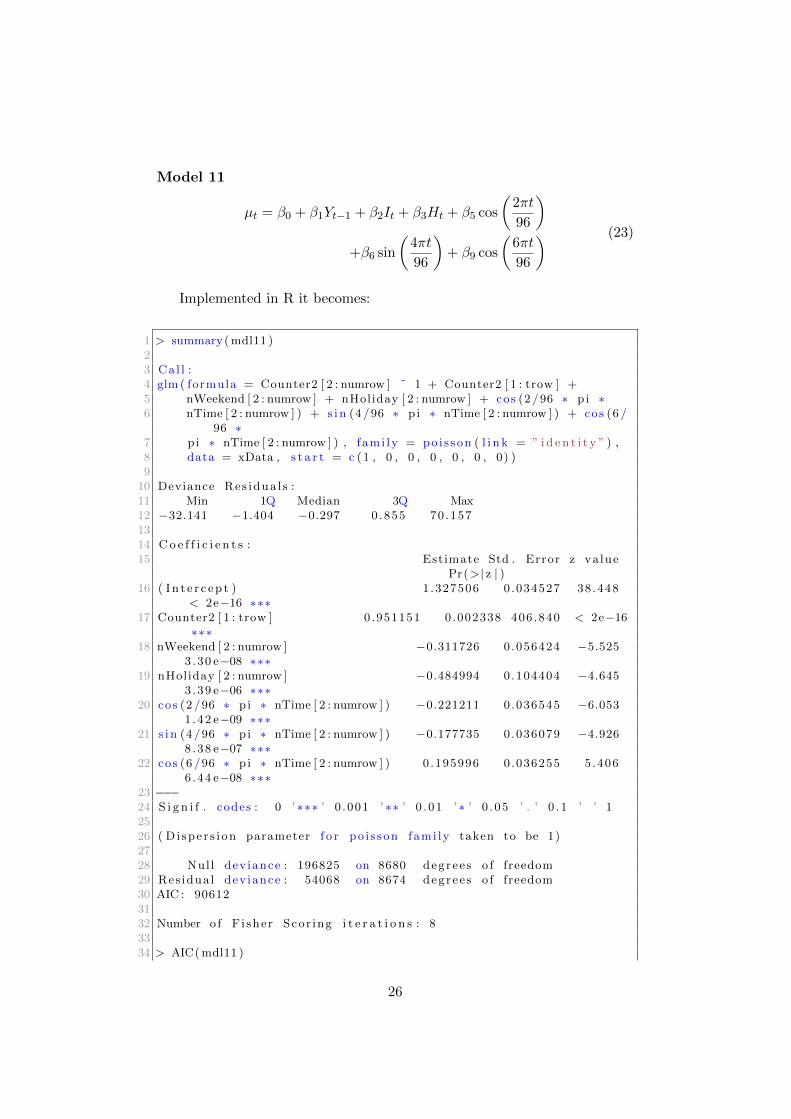
Model 11

µt = β0 + β1Yt−1 + β2It + β3Ht + β5 cos

(2πt

96

)+β6 sin

(4πt

96

)+ β9 cos

(6πt

96

) (23)

Implemented in R it becomes:

1 > summary(mdl11 )23 Ca l l :4 glm ( formula = Counter2 [ 2 : numrow ] ˜ 1 + Counter2 [ 1 : trow ] +5 nWeekend [ 2 : numrow ] + nHoliday [ 2 : numrow ] + cos (2 /96 ∗ pi ∗6 nTime [ 2 : numrow ] ) + s i n (4 /96 ∗ pi ∗ nTime [ 2 : numrow ] ) + cos (6 /

96 ∗7 p i ∗ nTime [ 2 : numrow ] ) , f ami ly = po i s son ( l i n k = ” i d en t i t y ” ) ,8 data = xData , s t a r t = c (1 , 0 , 0 , 0 , 0 , 0 , 0) )9

10 Deviance Res idua l s :11 Min 1Q Median 3Q Max12 −32.141 −1.404 −0.297 0 .855 70 .1571314 Co e f f i c i e n t s :15 Estimate Std . Error z value

Pr(>| z | )16 ( In t e r c ep t ) 1 .327506 0.034527 38 .448

< 2e−16 ∗∗∗17 Counter2 [ 1 : trow ] 0 .951151 0.002338 406.840 < 2e−16

∗∗∗18 nWeekend [ 2 : numrow ] −0.311726 0.056424 −5.525

3 .30 e−08 ∗∗∗19 nHoliday [ 2 : numrow ] −0.484994 0.104404 −4.645

3 .39 e−06 ∗∗∗20 cos (2 /96 ∗ pi ∗ nTime [ 2 : numrow ] ) −0.221211 0.036545 −6.053


8 .38 e−07 ∗∗∗22 cos (6 /96 ∗ pi ∗ nTime [ 2 : numrow ] ) 0 .195996 0.036255 5 .406

6 .44 e−08 ∗∗∗23 −−−24 S i g n i f . codes : 0 ’ ∗∗∗ ’ 0 .001 ’ ∗∗ ’ 0 .01 ’ ∗ ’ 0 .05 ’ . ’ 0 . 1 ’ ’ 12526 ( Di spe r s i on parameter f o r po i s son fami ly taken to be 1)2728 Nul l dev iance : 196825 on 8680 degree s o f freedom29 Res idua l dev iance : 54068 on 8674 degree s o f freedom30 AIC : 906123132 Number o f F i sher Scor ing i t e r a t i o n s : 83334 > AIC(mdl11 )

26

35 [ 1 ] 90611.7136 > BIC(mdl11 )37 [ 1 ] 90661.238 > l ogL ik (mdl11 )39 ’ l og Lik . ’ −45298.86 ( df=7)

Noticeable is that model 11 has both a lower AIC (90611.71) and BIC(90661.2) as well as all coefficients being significant with a p value lowerthen 0.001. This will be the model we settle for in this thesis, as a final steplets take a look at how model 11 are able to predict µt for counter 2:

0 500 1000 1500 2000

05

01

00

15

0

Time (15 minute interval)

Nu

mb

er

of

occu

rre

nce

s

Figure 12: Dotted gray is predicted value, black circle is measured value attime t

27

0 500 1000 1500 2000

−1

0−

50

51

01

52

0

Time (15 minute intervals)

Pe

ars

on

Re

sid

ua

l

Figure 13: Pearson Residuals

28

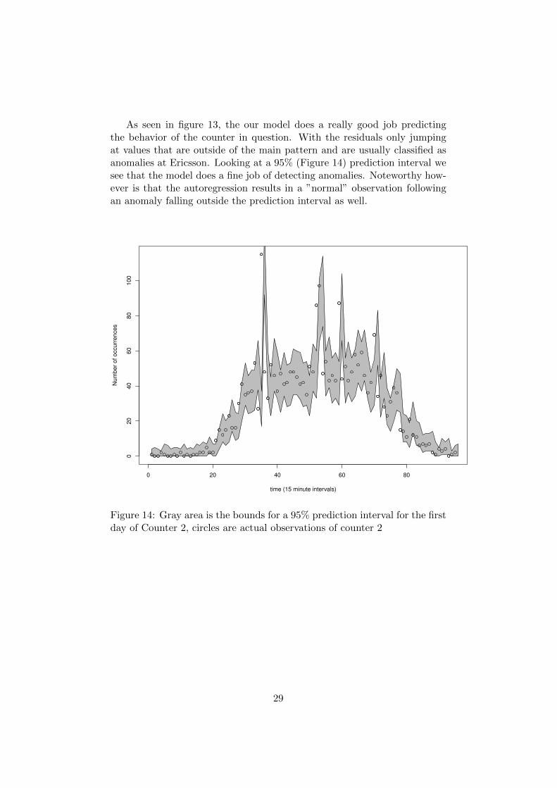
As seen in figure 13, the our model does a really good job predictingthe behavior of the counter in question. With the residuals only jumpingat values that are outside of the main pattern and are usually classified asanomalies at Ericsson. Looking at a 95% (Figure 14) prediction interval wesee that the model does a fine job of detecting anomalies. Noteworthy how-ever is that the autoregression results in a ”normal” observation followingan anomaly falling outside the prediction interval as well.

0 20 40 60 80

02

04

06

08

01

00

time (15 minute intervals)

Nu

mb

er

of

occu

rre

nce

s

Figure 14: Gray area is the bounds for a 95% prediction interval for the firstday of Counter 2, circles are actual observations of counter 2

29

5 Conclusion

We started out with data for four counters. After a short introduction inchapter 1 to how the network functions we then delved into data in detailtrying to display both the uniqueness and similarities of each counter vis-a-vis the others.

In chapter 2 we then covered generalized linear models and in particularthe Poisson model for count data that we intended to use for modeling. Wealso covered Parameter estimation and criteria we then went on to use toselect the best possible model. We then choose between 7 models, findingthe most complete one (model 4) to be the best. Then we expanded model4 into 3 more models attempting to model the daily cycle better by addingmore sin/cos terms. Choosing model 9 we then noticed that a few coeffi-cients where non significant we omitted these eventually settling on model11. We then took a look at how well model 11 would predict the first 3 weeksworth of data for counter 2. Judging from figure 13, the models ability ofpredicting µt was excellent.

The problem with the Poisson model for count data, is overdispersion,meaning that the variability in data will be greater then expected given ourmodel. One way to deal with this is to use an alternative, more complicated,model like the Negative-Binomial model or the Zeger-Qaqish model both ofwhich are discussed in Kedem and Fokianos (2002) and implemented in theR package tscount.

Possible future expansion of this work would be to consider if the coun-ters actually covariate, i.e. if a model for one counter using another counteras a covariate would yield even better results. Furthermore considering notjust additive covariates, but multiplicative ones as well and past predictionsare both viable expansion of the current model (model 11) in this thesis.Both of which I suspect would improve the fit.

From Ericssons point of view, implementing this work into an automatedanomaly detection scheme would prove very fruitful, at least based on ourexperiments in chapter 4. In this case comparing the ability of the abovementioned models ability to predict anomalies would again prove anotherinteresting extension of this thesis.

30

References

Ericsson Radio Systems AB (2001). Basic Concepts of WCDMA Radio Ac-cess Network. url: http://www.cs.ucsb.edu/~almeroth/classes/W03.595N/papers/wcdma-concepts.pdf.

Kedem, Benjamin and Konstantinos Fokianos (2002). Regression Models forTime Series Analysis. John Wiley & Sons, Inc. isbn: 0-471-36355-3.

Olsson, Ulf (2002). Generalized Linear Models - An Applied Approach. UlfOlsson and Studentlitteratur 2002. isbn: 978-91-44-03141-5.

Leonhard Held, Michael Hohle and Mathias Hofmann (2005). “A statisticalframework for the analysis of multivariate infectious disease surveillancecounts”. In: Statistical Modelling 5, pp. 187–191.

Hansen, Eric W. (2002). Fourier Transforms - Principles and Applications.John Wiley & Sons, Inc. isbn: 978-1-118-47914-8.

31

http://www.cs.ucsb.edu/~almeroth/classes/W03.595N/papers/wcdma-concepts.pdf

http://www.cs.ucsb.edu/~almeroth/classes/W03.595N/papers/wcdma-concepts.pdf

count data time series models for telecommunications data

Documents