counterfeit coins by jeﬀrey brown ... - physics.byu.edu

COUNTERFEIT COINS

by

Jeffrey Brown

A senior thesis submitted to the faculty of

Brigham Young University

in partial fulfillment of the requirements for the degree of

Bachelor of Science

Department of Physics and Astronomy

Brigham Young University

August 2007

BRIGHAM YOUNG UNIVERSITY

DEPARTMENT APPROVAL

of a senior thesis submitted by

Jeffrey Brown

This thesis has been reviewed by the research advisor, research coordinator,and department chair and has been found to be satisfactory.

Date Lawrence Rees, Advisor

Date Eric Hintz, Research Coordinator

Date Ross L. Spencer, Chair

ABSTRACT

COUNTERFEIT COINS

Jeffrey Brown

Department of Physics and Astronomy

Bachelor of Science

My research has been to try to establish and perfect non-destructive methods

to discern between counterfeit coins and genuine ones. I was able to use XRF

spectroscopy to develop methods of identifying incorrect materials in coins,

incorrect proportions of materials in coins, and even invalid claims to ages of

coins. I used an electron-microscope to identify minute alterations such as

tampering with mint marks and/or dates. These methods greatly increase the

ability to determine if a coin is counterfeit without damaging the coins.

ACKNOWLEDGMENTS

I would like to acknowledge Dr. Rees for all of his help in guiding me

through trouble spots throughout my research. The physics department must

receive credit for giving me the requirement to write this; it really taught me a

lot about writing technical papers. The coin dealer receives thanks for lending

us all of these coins to do the experiments with for so long.

Contents

Table of Contents vii

List of Figures ix

1 Introduction 11.1 Counterfeit Coins . . . . . . . . . . . . . . . . . . . . . . . . . . . . . 11.2 Counterfeiting Methods . . . . . . . . . . . . . . . . . . . . . . . . . 11.3 Counterfeit Detection . . . . . . . . . . . . . . . . . . . . . . . . . . . 31.4 Elemental Analysis . . . . . . . . . . . . . . . . . . . . . . . . . . . . 41.5 My Research . . . . . . . . . . . . . . . . . . . . . . . . . . . . . . . . 5

2 Experimental Methods 72.1 XRF Spectroscopy . . . . . . . . . . . . . . . . . . . . . . . . . . . . 72.2 Using Standards . . . . . . . . . . . . . . . . . . . . . . . . . . . . . . 102.3 Target Selection . . . . . . . . . . . . . . . . . . . . . . . . . . . . . . 112.4 Accuracy Checks . . . . . . . . . . . . . . . . . . . . . . . . . . . . . 112.5 Additional Check . . . . . . . . . . . . . . . . . . . . . . . . . . . . . 13

3 Results 153.1 Repeatability . . . . . . . . . . . . . . . . . . . . . . . . . . . . . . . 153.2 Physical Variation . . . . . . . . . . . . . . . . . . . . . . . . . . . . . 163.3 Age Variation . . . . . . . . . . . . . . . . . . . . . . . . . . . . . . . 173.4 Additional Check . . . . . . . . . . . . . . . . . . . . . . . . . . . . . 18

4 Analysis of Results 214.1 Physical and Time Variation . . . . . . . . . . . . . . . . . . . . . . . 214.2 Age Variation . . . . . . . . . . . . . . . . . . . . . . . . . . . . . . . 224.3 Additional Check . . . . . . . . . . . . . . . . . . . . . . . . . . . . . 234.4 Conclusion . . . . . . . . . . . . . . . . . . . . . . . . . . . . . . . . . 23

Bibliography 27

vii

List of Figures

2.1 1964 U.S. Half Dollar . . . . . . . . . . . . . . . . . . . . . . . . . . . 8

3.1 Ni to Ti conversion . . . . . . . . . . . . . . . . . . . . . . . . . . . . 163.2 Copper in the Three Coins . . . . . . . . . . . . . . . . . . . . . . . . 173.3 Silver in the Three Coins . . . . . . . . . . . . . . . . . . . . . . . . . 183.4 Copper in the 18 Dimes . . . . . . . . . . . . . . . . . . . . . . . . . 193.5 Silver in the 18 Dimes . . . . . . . . . . . . . . . . . . . . . . . . . . 19

4.1 Counterfeit Mint Mark . . . . . . . . . . . . . . . . . . . . . . . . . . 25

ix

Chapter 1

Introduction

1.1 Counterfeit Coins

The first known use of coins was circa 550 B.C. in the kingdom of Lydia in modern

day Turkey. Before the advent of coins, the economy was based on bartering. You

could only get what you wanted from someone if you had something that they wanted.

Coins were invented as a form of currency to enable trading between more people.

A widely accepted coin would let you trade anything with anyone. People have been

making counterfeit coins for as long as real ones have been used. My research has been

to try to establish and perfect non-destructive methods to discern between counterfeit

coins and genuine ones.

1.2 Counterfeiting Methods

There are many ways to counterfeit coins, and some methods are much better than

others. Cutting out a picture of a quarter and taping it to a penny is not very

convincing, but some counterfeits are quite deceptive. You could actually get the

1

2 Chapter 1 Introduction

materials you would need to make a coin and manufacture a coining press to make

your own coins, but that is a little more work than most people are willing and

capable of doing. Counterfeiters are more likely to try and take relatively worthless,

real coins and alter them slightly, making them look like far more valuable coins.

Changing minute things, like mint marks or dates, is far simpler than making entire

coins from scratch and the results can be very difficult to spot with the naked eye.

For these situations, there needs to be a better way than just simply looking at a coin

to determine if it is counterfeit.

Another particularly big problem with counterfeit coins is with very old coins.

Before machine presses and advanced tools, the methods for creating coins were crude

and often times inconsistent. Any average Joe could make dyes in his back yard and

strike a coin with a hammer, because that is exactly how it was done back then. An

accurate counterfeit detecting procedure will need to identify these types of scenarios

and provide a way to determine the age of a coin. In the past century, coin making

methods have gotten much more specialized and difficult to duplicate. The aging

process also has an effect on coins. We need some way of looking at them that is

better than just putting them under a magnifying glass for examination. There are

details that even great magnifying glasses may not make discernable.

If, for example, someone wanted to counterfeit a coin and make it look like a real

coin so they could use it in trade (more popular when coins were the primary currency

used), then they would probably make it out of a material that is less valuable than

the silver or gold out of which the real coins were made; or at least, less of those

precious metals. Often, people would simply shave off the very outer ring of a coin

so it would not alter the face of the coin. Governments started reeding their coins

(placing ridges around the edge) to prevent this sort of tampering. Sometimes, they

even cut open a real coin and scraped out some of the silver from the middle and

1.3 Counterfeit Detection 3

filled it with something else of far less value, like lead or copper.

1.3 Counterfeit Detection

There are many aspects of a coin to take into consideration when determining whether

it is real or not: the most important are composition, color, shape, and weight. The

latter three are generally easily spotted (depending on the extent of the tampering)

and most people can tell without too much difficulty whether a coin is the right color,

shape, and weight. Things like scratching off mint marks, or adding on new ones

that were not already there, or changing dates to make them appear older should be

visibly noticeable. If the coin was sliced down the center and later resealed, I should

see the new seal. There are other methods of “looking at” these coins than what the

coin collectors use now.

An electron-microscope is very good at “looking at” very minute details. It can

magnify up to thousands of times actual size with very good resolution. One of the

more capable aspects of an electron-microscope is that it can use x-ray analysis to

determine, with limited accuracy, the composition of a very small region of interest.

Composition is difficult to detect accurately.

Some counterfeiters may be able to make a coin that can get by even the sharp eye

of a coin dealer. Even he cannot tell exactly what a coin is made of just by looking at

it. Checking the composition of such coins would be very useful in determining if a

coin is counterfeit or not. This would indicate if it is made of the correct proportions

of the specific elements as well as if the coin is as old as it is claims to be. However,

as coins get older and are used over and over again, the composition of the coin can

change. For example, if you had a coin made of a mixture of copper and silver, the

silver in the coin is very stable and does not react well with its surroundings. The


copper on the other hand, would corrode, oxidize, and rub away onto your hands.

That should mean that the surface of the coin would have a lower concentration of

copper than it had originally. If a coin claims to have been in circulation for 100 years,

when I check its composition, I should notice a significantly smaller concentration of

copper when compared to a 50-year old coin.

1.4 Elemental Analysis

There is a variety of methods and machines that can be used to determine just what

elements a sample contains. A particularly useful one is the X-Ray Fluorescence

spectrometer. When a material is exposed to high energy x rays, some of its atoms

become ionized. If the x rays have enough energy, they can even eject the more tightly

bound, inner orbital electrons. When this happens, it renders the atom unstable and

the higher orbital electrons are then able to “fall” down into the lower or inner orbitals.

When this happens, the higher orbital electron must give off energy in the form of an x

ray. That x ray has precisely the energy difference between the two orbitals involved.

The term fluorescence is applied to phenomena wherein higher energy radiation is

absorbed, stimulating the emission of lower energy radiation. That is why it is called

X-Ray Fluorescence or XRF. [1]

XRF spectrometers have been used for a very long time to analyze all kinds of

samples. The x rays that come out of the sample have very precise energy levels that

are like a fingerprint of the particular element they came from. That means that if

you can detect all of the x rays coming out, you can tell just what a sample is made

of to a better accuracy than an electron-microscope can.

1.5 My Research 5

1.5 My Research

My research has been to try to establish and perfect non-destructive methods to

discern between counterfeit coins and genuine ones. I will describe how I analyzed

coins counterfeited in different ways. Using these methods of detection, I determined

not only whether each of these coins is counterfeit, but also exactly what it was that

made them counterfeit. If it has been cut in half and shaved out a bit, I noticed it.

If the mint mark was made out of a different material, I spotted it. If the coin is not

as old as it claims it is, I was able to determine that. If the coin is made with the

wrong proportions of constituents, I was able to figure that out as well.

I was able to determine exactly which coins are real and which are counterfeit

without damaging them a bit. I will describe in more detail the use of electron

microscopy and x-ray fluorescence spectroscopy for this purpose. There are a few

tricky details that needed to be taken into consideration when dealing with XRF.

Chapter 2

Experimental Methods

There were several experiments that needed to be conducted in order to research the

capabilities of proper counterfeit detection methods. At the peak of most of them

was the XRF spectrometer. With it I determined the limitations and capabilities of

counterfeit detection. The electron microscope was also a useful tool in analyzing

smaller details that the XRF could not detect. This chapter explains the various

experiments that were conducted to develop these methods.

2.1 XRF Spectroscopy

I used an XRF spectrometer to analyze the elemental composition of several samples,

both authentic and counterfeit. I will discuss briefly how the spectrometer works since

I used it for many different experiments. The primary x rays are produced in an x-ray

tube, called the source. The source produces x rays by accelerating electrons through

voltages as large as 60kV, and then allows the electrons to strike a ruthenium plate.

The electrons rapidly decelerate when they strike the plate, producing x rays through

the bremsstrahlung process. The bremsstrahlung x rays then strike a thin foil called

7

8 Chapter 2 Experimental Methods

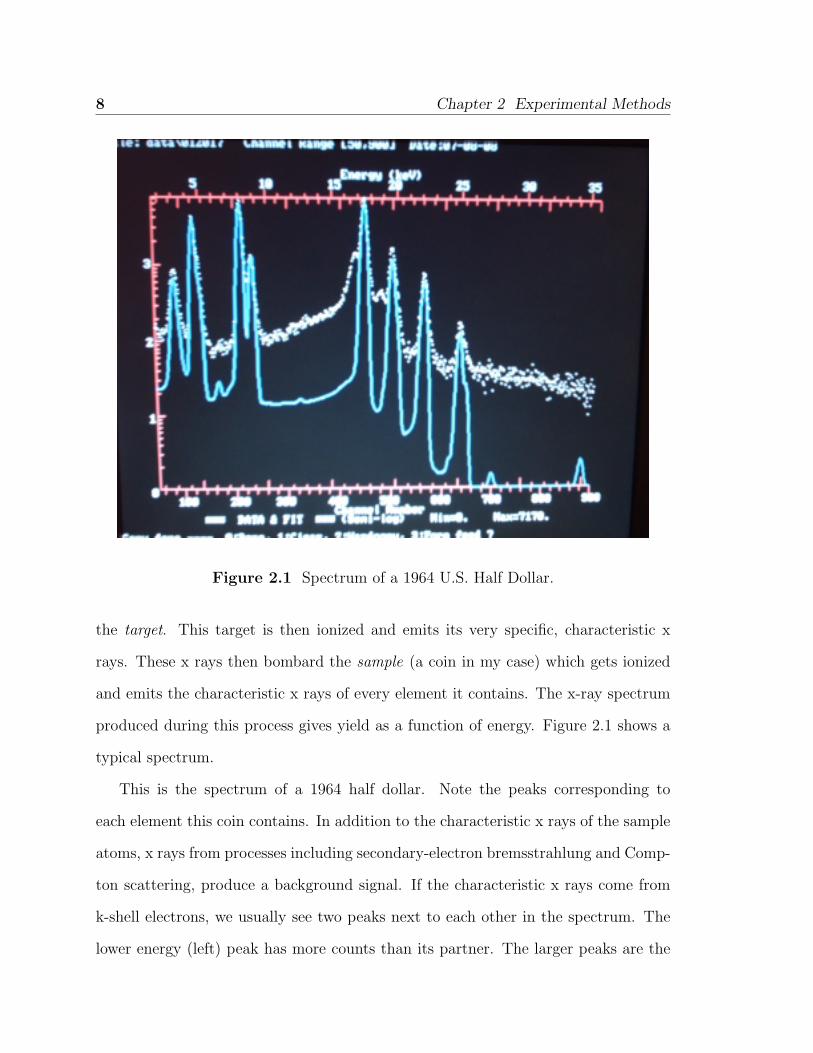
Figure 2.1 Spectrum of a 1964 U.S. Half Dollar.

the target. This target is then ionized and emits its very specific, characteristic x

rays. These x rays then bombard the sample (a coin in my case) which gets ionized

and emits the characteristic x rays of every element it contains. The x-ray spectrum

produced during this process gives yield as a function of energy. Figure 2.1 shows a

typical spectrum.

This is the spectrum of a 1964 half dollar. Note the peaks corresponding to

each element this coin contains. In addition to the characteristic x rays of the sample

atoms, x rays from processes including secondary-electron bremsstrahlung and Comp-

ton scattering, produce a background signal. If the characteristic x rays come from

k-shell electrons, we usually see two peaks next to each other in the spectrum. The

lower energy (left) peak has more counts than its partner. The larger peaks are the

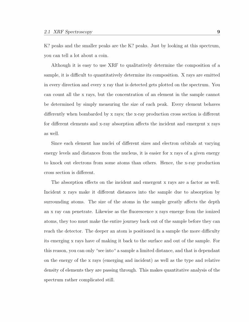
2.1 XRF Spectroscopy 9

K? peaks and the smaller peaks are the K? peaks. Just by looking at this spectrum,

you can tell a lot about a coin.

Although it is easy to use XRF to qualitatively determine the composition of a

sample, it is difficult to quantitatively determine its composition. X rays are emitted

in every direction and every x ray that is detected gets plotted on the spectrum. You

can count all the x rays, but the concentration of an element in the sample cannot

be determined by simply measuring the size of each peak. Every element behaves

differently when bombarded by x rays; the x-ray production cross section is different

for different elements and x-ray absorption affects the incident and emergent x rays

as well.

Since each element has nuclei of different sizes and electron orbitals at varying

energy levels and distances from the nucleus, it is easier for x rays of a given energy

to knock out electrons from some atoms than others. Hence, the x-ray production

cross section is different.

The absorption effects on the incident and emergent x rays are a factor as well.

Incident x rays make it different distances into the sample due to absorption by

surrounding atoms. The size of the atoms in the sample greatly affects the depth

an x ray can penetrate. Likewise as the fluorescence x rays emerge from the ionized

atoms, they too must make the entire journey back out of the sample before they can

reach the detector. The deeper an atom is positioned in a sample the more difficulty

its emerging x rays have of making it back to the surface and out of the sample. For

this reason, you can only “see into“ a sample a limited distance, and that is dependant

on the energy of the x rays (emerging and incident) as well as the type and relative

density of elements they are passing through. This makes quantitative analysis of the

spectrum rather complicated still.


2.2 Using Standards

Because of these complicating factors, the method of determining the actual amounts

of an element in a particular sample involves the use of standards. If you had a sample

that contained only copper and silver, you could compare its spectrum to samples

having known proportions of those elements. If you had a known sample that had

a very similar consistency, you could then infer its composition. Since it is difficult

to find standards of precisely the right composition, I needed a more elegant way of

approaching these samples.

I then needed to develop a suitable method of comparing a sample coin with

standards. First, the total number of counts in a spectral peak is not very meaningful

by itself. If we simply run the spectrometer a little longer, we would have more

counts in all of our peaks; which obviously does not imply that we have more of every

element. Run time cannot be a factor. I found a way of normalizing the data so

that different sets can be compared to each other accurately. I used a standard for

comparison that was fixed in every set of data. The standard was a thin wire placed

below every sample so that it could not be affected by any given sample’s cross section

or its absorption effects. It was hit by the exact same fraction of the total incident x

rays during each run. I compared each element of the sample to the same element in

the standard, and every standard element could in turn be compared to all the other

standards in other runs. This was the connection between runs that was necessary

to compare separate spectra.

One problem with this method was if the standard I chose was a constituent or even

a neighboring element to a constituent in my sample, the peaks would interfere with

each other. Then the standard would not be comparable to those in other spectra.

The solution to this problem was finding another standard elementally dissimilar to

2.3 Target Selection 11

the sample and the previous standard. As long as I run the two samples alone to

find out how they compare to each other, I can always convert from one to the other.

For my standards, I chose nickel and titanium (both 0.999 pure) and fastened them

directly over the center of the slide whereon the samples lie.

2.3 Target Selection

Another important consideration is the proper selection of the target. Since the x

rays that strike the target are primarily the characteristic x rays of the target foil, the

choice of target is based on the energy of x rays that are best suited to the sample. If

the x rays are too low in energy, they will not ionize the target. If the x rays are too

high in energy, they produce more background and can obscure small peaks. I have

chosen molybdenum to be my target, for there are no elements near it found in any of

my coins and it has sufficient energy in its emitted x rays to ionize any element that

any coin may contain. That also implies that there will be a large peak corresponding

to molybdenum x rays in all of my spectra.

2.4 Accuracy Checks

Now that we have a good consistent method to use to acquire and analyze data,

I felt that it was important to figure out the accuracy of our measuring capabilities.

There are four ways that I decided to test the samples to determine this: repeatability,

physical variations, time variations, and age variations. Let me explain what I mean

by each of those.

Checking to see the degree to which the XRF is repeatable is the most important


thing to check. If I do a run on a given coin and immediately afterwards do that

exact same run again, I should get the same results. Obviously, it is impossible

to get exactly identical results experimentally, but I need to see how consistent the

spectrometer is. To test this, I chose to compare my nickel standard and my titanium

standard. Five times I analyzed the Ni wire immediately adjacent to the Ti strip,

both very close to the center of the sampling region.

Checking the physical variations was a little tricky. If I take the coin that was

originally heads up and flip it over to be face down, the x rays will be incident on

a different surface. I needed to see how much that would affect the x ray spectrum.

Perhaps the x rays may bounce off differently or get absorbed in a different manner

due to the contours on the surface. It is important to know whether putting my

coin in slightly rotated will give me different results. This was tested by taking three

different coins (a half dollar, a quarter, and a dime) from the same year and taking

various runs with them. I took two runs of each coin with the reverse (tail) side up

and the obverse (head) oriented upright when viewed from above. Then, I ran them

each a third time with them rotated 180 degrees such that each coin was still reverse

up, but upside down. I also took a fourth run of each coin while flipped over to make

them obverse up with the head right side up. This checked to see how much physical

variations changed the spectra.

Another factor that I felt may be important was time. Are the XRF results

consistent in time? To test this, I took the very same three coins I used in testing

physical variations and ran them each one final time several weeks later. I ran them

all in the same position as each other and in the same position that I started the last

experiment in: reverse up and upright. This checked for any discrepancies that arise

as a result of taking different runs at different time periods to allow comparison of

spectra that have been taken at varying intervals throughout the course of this entire

2.5 Additional Check 13

experiment.

The last type of accuracy I felt was important to check for was a very significant

one: age. There was a concern that the proportions of a coin’s constituents would

change over time just from being in circulation (as I mentioned in Chapter 1). To

approach this, I took coins from different periods of time (eighteen dimes with ranging

from 1899 to 1963) to examine their copper and silver levels. I expected some variation

in composition due to the different history of each coin. Then, I compared their copper

levels to observe any trend lines that could lead me to be able to compare older coins

to newer ones. With the oldest coin twice as old as the newest one, I was able to

notice how age affected the proportions of constituents.

2.5 Additional Check

Upon investigating the physical variations experiment among the half dollar, quarter

and dime, there was an identifiable feature that led to an additional check. For some

reason the dime was different somehow from the half dollar and quarter (which were

similar to each other- as discussed in the next chapter). There is a finite area of

incidence where the x rays interact with the sample. Due to the varying sizes of

coins, it was important to know how that size compared to my coins. To do this,

I placed a gold coin, smaller than even the dime, behind each of the coins and ran

them again to observe if the gold could be “seen.“ I also ran each of them with a lead

coin, larger than even the half dollar, behind each of the coins for the same purpose.

This experiment enabled me to decipher which of the coins was “infinitely thick“ or

“infinitely wide.“

Having completed all of these consistency checks for repeatability, physical vari-

ations, time variations, and age variations, I was able to compare quite well the


different spectra together in a way that not previously done.

Chapter 3

Results

Upon completion of the few experiments discussed in Chapter 2, the data were col-

lected and analyzed. The forms of analysis that I found most useful are described in

this chapter. The analysis of these results (with the exception of the first experiment)

will be reserved until the following chapter. It is important to note for each if these

results, if not otherwise specified, the coins all originally contained 90% silver and

10% copper. That includes the dimes, quarters, and half dollars for the entire range

of dates I have chosen [2].

3.1 Repeatability

We will first discuss the results of the accuracy checks described in Section 2.4. First,

I took my two standard wires (Ti and Ni) and ran them together to analyze their

relation. I ran them five times, each time a little longer than the time before in order

to ensure the ratio between the two would remain a constant independent of run

time. These data were all taken with a molybdenum target. Figure 3.1 shows that

each run, due to their varying lengths of time, had very different Ni and Ti counts.

15

16 Chapter 3 Results

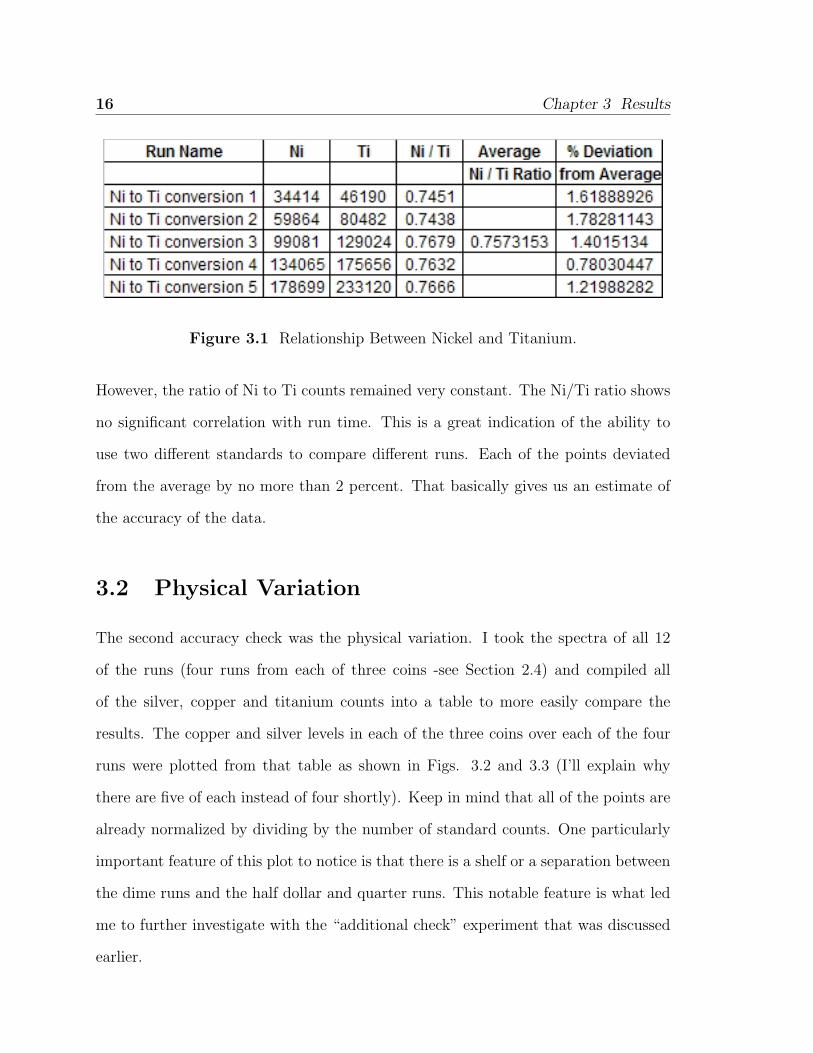
Figure 3.1 Relationship Between Nickel and Titanium.

However, the ratio of Ni to Ti counts remained very constant. The Ni/Ti ratio shows

no significant correlation with run time. This is a great indication of the ability to

use two different standards to compare different runs. Each of the points deviated

from the average by no more than 2 percent. That basically gives us an estimate of

the accuracy of the data.

3.2 Physical Variation

The second accuracy check was the physical variation. I took the spectra of all 12

of the runs (four runs from each of three coins -see Section 2.4) and compiled all

of the silver, copper and titanium counts into a table to more easily compare the

results. The copper and silver levels in each of the three coins over each of the four

runs were plotted from that table as shown in Figs. 3.2 and 3.3 (I’ll explain why

there are five of each instead of four shortly). Keep in mind that all of the points are

already normalized by dividing by the number of standard counts. One particularly

important feature of this plot to notice is that there is a shelf or a separation between

the dime runs and the half dollar and quarter runs. This notable feature is what led

me to further investigate with the “additional check” experiment that was discussed

earlier.

3.3 Age Variation 17

Figure 3.2 Copper in the Three Coins.

The time factor was the third accuracy check that I felt was important. After

running each of the three coins one last time, I simply plotted their normalized silver

and copper levels to be consistent with the earlier runs. That is why there are 15

in the figure instead of 12. For each of the three coins we had the coin reverse side

up twice with the image upright, then once rotated 180 degrees still reverse side up,

followed by flipping the coin with the obverse side up and upright. The fifth run was

done several weeks later, making 15 runs total.

3.3 Age Variation

The last accuracy check I made was one to determine how age affected a particular

coin to the point of altering its physical make up. After running the 18 coins, I took

the same data as in the last experiments and plotted them in the next two figures.

Figure 3.4 shows the normalized copper in the 18 different coins plotted against the

years they were made; whereas Fig. 3.5 shows the same but with the silver instead


Figure 3.3 Silver in the Three Coins.

of copper.


The half dollars, quarters and dimes are all made of identical proportions of silver

and copper and are all normalized to the same titanium, yet they look different in

Fig. 3.2. There is the factor of penetration distance within the varying coins. Upon

analyzing the spectra resulting from having a small gold coin behind each of my coins,

none of them showed any traces of gold. The second half of this experiment was with

the large lead coin placed behind each of the three coins. The lead showed up only in

the spectrum with the dime and in neither of the other two: half dollar and quarter.

With all of the data and plots that were just shown, I was able to infer many

results that lead me to be able to analyze coins to determine if they are counterfeit.


Figure 3.4 Copper in the 18 Dimes.

Figure 3.5 Silver in the 18 Dimes.

Chapter 4

Analysis of Results

Now I will discuss how I interpreted the data. I will explain them in the order they

were presented. Then I will discuss the conclusions I have drawn and how they can

be applied to counterfeit detection.

4.1 Physical and Time Variation

The copper from the physical variations experiment plotted with the time variation

experiment (Fig. 3.2) demonstrates a very reasonable result. You will notice that all

of the half dollar points look very consistent as do the quarter and dime points, at

least among themselves. These variations are due to varying runs and apparently not

to differences in coin designs or patterns. This tells me that it does not matter which

face of the coin I am looking at, nor should it matter which angle it is positioned at.

Any way it is placed in the XRF spectrometer should yield the same results. Waiting

for a few weeks in between runs does not make a difference as well which implies that

I can compare different coins from differing months to each other without worrying.

21

22 Chapter 4 Analysis of Results

4.2 Age Variation

Looking at the results of the age variation in Fig. 3.5 there is not a correlation

between age and amount of silver remaining in the different dimes. This tells me

one of three things: either the amount of silver in each of the dimes is remaining

constant, increasing as they get older permitting the x ray to penetrate less deeply,

or decreasing as time goes on allowing them to penetrate further. Obviously the

amount of silver cannot be increasing as the coins get older, but either of the other

two may be valid.

On the other hand, if we take a look at the copper in Fig. 3.4, we observe a

correlation indeed between the amount of copper in the coin and its age. The copper

levels are lower for the older coins. This could mean only one of two things: either

the copper levels in the coins really are decreasing as the coins get older, or they are

remaining constant and the silver levels in the newer coins are lower (allowing the x

rays to penetrate deeper and “spot“ more copper). There cannot be less silver in the

newer coins, so we can conclude that the amount of copper decreases over time.

This leaves two possible solutions that would satisfy both plots. That means

either the silver remains constant and the copper decreases as time goes on, or both

the silver and the copper decrease over time. Silver is a much more stable element

that does not react very easily with other elements, but copper is much more likely

to be corroded and rubbed off onto peoples’ hands as the coin is used and handled.

These results lead me to conclude that the copper in the coin does in fact decrease

as the coin gets older, but that the amount of silver remains constant.



The first half of the additional check (see Sections 2.5 and 3.4) showed that the gold

could not be seen through the half dollar, the quarter, or the dime. That implies that

none of the x rays made it all the way through any of the coins which allows us to

define all of them to be “infinitely thick.“ The second half of the experiment showed

that the lead was seen in the spectrum of the dime but not the other two coins. This

could be one of two things, whether I saw the lead around the dime or through it.

Considering the results of the first half of this experiment, I ruled out the latter of

those two options and am convinced that the lead was seen around the sides of the

dime. That means that the area of incidence is larger than a dime, but smaller than

a quarter or a half dollar. This would explain perfectly why there are fewer copper

and fewer silver counts in the dime than there were in the other two coins. Many of

the x rays that would normally strike the quarter or the half dollar would not hit the

dime. However, exactly the same percentage of the x rays will still strike the titanium

standard. Upon normalizing to that same titanium strip, the dime appears to have

fewer counts. That is why there is a “shelf” in those two plots.

4.4 Conclusion

Now that I have successfully tested the XRF spectrometer, I can determine if a coin

has the correct composition for a genuine coin using the methods I have explained.

The most important check is the simplest one of all: whether the coin is made of the

correct materials. The XRF can handle that with very little trouble. If the coin is

made of the wrong proportions of the right materials, the coins that I have previously

analyzed give me a good basis for determining those ratios. If the coin is made of

the correct proportions of the correct materials, then it may be much newer than it


claims to be. I can test to see how its age compares to my age curve to see if it can

indeed be as old as it claims. If that also is correct, than it very likely is a genuine

coin; however, someone may have tampered with it (changing mint marks or dates

for example). Then we should be able to see tool markings or scratches of some sort

in an electron microscope. If no such markings can be seen, x-ray analysis with an

electron microscope can check the elemental composition of the mint marks alone or

the dates and compare them to the rest of the coin and see if they have identical

constituents. If they pass these tests, there remains the possibility that the coin was

struck counterfeit made of precisely the correct materials. However, we can eliminate

a large fraction of the types of counterfeits encountered by using these techniques.

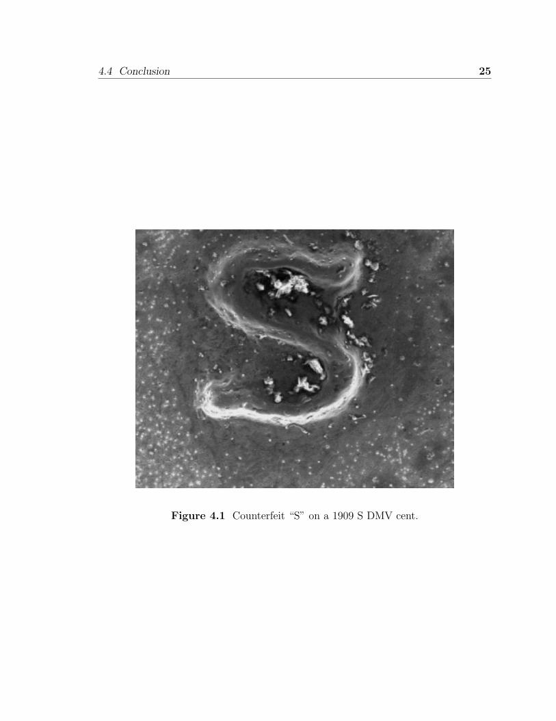
Figure 4.1 is an example of a coin that has minute details altered. It is a 1916

dime that has a counterfeit “D” that was placed on it to raise the value of the coin.

You can see that it is very difficult to notice flaws in such a well made mint mark,

that without the aid of an electron microscope, it would be difficult to notice.

4.4 Conclusion 25

Figure 4.1 Counterfeit “S” on a 1909 S DMV cent.

Bibliography

[1] Amptek Inc., “X-Ray Fluorescence (XRF),” http://www.amptek.com/pdf/xrf.

pdf (Accessed July 22, 2007).

[2] R. S. Yeoman, A Guide Book of United States Coins: The Official Red Book,

53rd ed. (New York, N. Y., 1999), p. 128.

27

http://www.amptek.com/pdf/xrf.pdf



counterfeit coins by jeﬀrey brown ... - physics.byu.edu

Documents