Counting Cars and Determiningthe Vacancy of a Parking Lot

using Neural Networks

Alexander Holmstrom

June 6, 2018Master’s Thesis in Computing Science, 30 creditsInternal Supervisor at CS-UmU: Michael Minock

External Supervisor at Knowit: Andreas HedExaminer: Henrik Bjorklund

Umea UniversityDepartment of Computing Science

SE-901 87 UmeaSweden

Abstract

A lot of time, energy and money is being wasted when people are trying tofind a parking lot. These elements could be reduced if the driver is providedvacancy information of a parking lot beforehand. In this thesis Google’s ObjectDetection API is implemented and two pre-trained models are being used onthe PKLot dataset to detect and count the number of cars in a parking lot. Themodels are based on a Region-based Convolutional Neural Network (R-CNN)which is explained in more detail. The models are compared with each otherand its result presented. The result is presented with three factors in focus,the number of predictions made by the models, the number of cars a modelmissed to predict and how many objects that were wrongfully predicted. Thiswas then tested on a Raspberry PI with the purpose to avoid using a remotecomputer for the image processing and prevent potential laws regarding camerasurveillance. Finally, we determine if this functionality can actually be deliveredusing state-of-the-art technology.

Contents

1 Introduction 1

2 Background 32.1 What is a Neural Network . . . . . . . . . . . . . . . . . . . . . . 32.2 Convolutional Neural Network (CNN) . . . . . . . . . . . . . . . 4

2.2.1 Problem Space . . . . . . . . . . . . . . . . . . . . . . . . 52.2.2 Inputs and Outputs . . . . . . . . . . . . . . . . . . . . . 5

2.3 Structure of a CNN[6][7] . . . . . . . . . . . . . . . . . . . . . . . 62.3.1 Convolutional Layer . . . . . . . . . . . . . . . . . . . . . 62.3.2 Non-linear Layer . . . . . . . . . . . . . . . . . . . . . . . 102.3.3 Pooling Layer . . . . . . . . . . . . . . . . . . . . . . . . . 102.3.4 Dropout Layer[12] . . . . . . . . . . . . . . . . . . . . . . 112.3.5 Fully Connected Layer . . . . . . . . . . . . . . . . . . . . 11

2.4 Training a CNN . . . . . . . . . . . . . . . . . . . . . . . . . . . . 122.4.1 Backpropagation . . . . . . . . . . . . . . . . . . . . . . . 12

2.5 Testing the CNN . . . . . . . . . . . . . . . . . . . . . . . . . . . 142.6 Region-based CNN[15] . . . . . . . . . . . . . . . . . . . . . . . . 14

2.6.1 R-CNN[16] . . . . . . . . . . . . . . . . . . . . . . . . . . 142.6.2 Fast R-CNN[20] . . . . . . . . . . . . . . . . . . . . . . . 152.6.3 Faster R-CNN[23] . . . . . . . . . . . . . . . . . . . . . . 16

3 Approach 183.1 TensorFlow . . . . . . . . . . . . . . . . . . . . . . . . . . . . . . 183.2 Google’s Object Detection API in TensorFlow[27] . . . . . . . . . 183.3 Dataset . . . . . . . . . . . . . . . . . . . . . . . . . . . . . . . . 18

3.3.1 PKLot Dataset . . . . . . . . . . . . . . . . . . . . . . . . 193.3.2 COCO Dataset . . . . . . . . . . . . . . . . . . . . . . . . 21

3.4 Models . . . . . . . . . . . . . . . . . . . . . . . . . . . . . . . . . 213.5 Evaluation . . . . . . . . . . . . . . . . . . . . . . . . . . . . . . . 223.6 Raspberry PI . . . . . . . . . . . . . . . . . . . . . . . . . . . . . 22

4 Experiments 234.1 Methods . . . . . . . . . . . . . . . . . . . . . . . . . . . . . . . . 234.2 Box Optimization . . . . . . . . . . . . . . . . . . . . . . . . . . . 24

4.3 Additional Training . . . . . . . . . . . . . . . . . . . . . . . . . 244.4 Method 1 . . . . . . . . . . . . . . . . . . . . . . . . . . . . . . . 254.5 Method 2 . . . . . . . . . . . . . . . . . . . . . . . . . . . . . . . 264.6 Method 3 . . . . . . . . . . . . . . . . . . . . . . . . . . . . . . . 264.7 Method 4 . . . . . . . . . . . . . . . . . . . . . . . . . . . . . . . 27

5 Result 285.1 Method 1 . . . . . . . . . . . . . . . . . . . . . . . . . . . . . . . 295.2 Method 2 . . . . . . . . . . . . . . . . . . . . . . . . . . . . . . . 305.3 Method 3 . . . . . . . . . . . . . . . . . . . . . . . . . . . . . . . 305.4 Method 4 . . . . . . . . . . . . . . . . . . . . . . . . . . . . . . . 315.5 Summary of Results . . . . . . . . . . . . . . . . . . . . . . . . . 325.6 Extra Experiment . . . . . . . . . . . . . . . . . . . . . . . . . . 33

6 Discussion 346.1 Reasons for Unsatisfying Result . . . . . . . . . . . . . . . . . . . 34

6.1.1 Training . . . . . . . . . . . . . . . . . . . . . . . . . . . . 346.1.2 Prediction . . . . . . . . . . . . . . . . . . . . . . . . . . . 346.1.3 Overfitting . . . . . . . . . . . . . . . . . . . . . . . . . . 346.1.4 Dataset . . . . . . . . . . . . . . . . . . . . . . . . . . . . 356.1.5 Models . . . . . . . . . . . . . . . . . . . . . . . . . . . . 35

6.2 Determining Occupied Parking Spaces . . . . . . . . . . . . . . . 356.3 Other Areas for Neural Networks . . . . . . . . . . . . . . . . . . 366.4 How Companies use CNNs . . . . . . . . . . . . . . . . . . . . . . 37

7 Conclusion 38

Appendix A Additional Graphs from the Result 42

List of Figures

1.1 The parking lot used. . . . . . . . . . . . . . . . . . . . . . . . . 2

2.1 Perceptron neural network. . . . . . . . . . . . . . . . . . . . . . 42.2 Convolutional Neural Network. . . . . . . . . . . . . . . . . . . . 52.3 What the human sees(left) and what the computer sees(right). . 52.4 A 5x5 filter convolving around an image representation and pro-

ducing a feature map. . . . . . . . . . . . . . . . . . . . . . . . . 72.5 The pixel(left) and non-pixel representation of the filter(right). . 72.6 The original image(left) and the image with a filter(right). . . . . 82.7 Visualization of the multiplication between the input image and

the filter being on a curve. . . . . . . . . . . . . . . . . . . . . . . 82.8 Visualization of the multiplication between the input image and

the filter not being on a curve. . . . . . . . . . . . . . . . . . . . 82.9 The input(left) with an input size of 7x7, filter size of 3x3 and

stride 1 resulting in an output(right) of size 5x5. . . . . . . . . . 92.10 The input(left) with an input size of 7x7, filter size of 3x3 and

stride 2 resulting in an output(right) of size 3x3. . . . . . . . . . 102.11 Example of max pooling with a 2x2 filter and a stride of 2. . . . 112.12 Visualization of gradient descent on a set of different level sets. . 132.13 Visualization of when the learning rate is too high(left) and when

the learning rate is small(right). . . . . . . . . . . . . . . . . . . . 142.14 Visualization of the steps in a R-CNN. . . . . . . . . . . . . . . . 152.15 Visualization of a Fast R-CNN. . . . . . . . . . . . . . . . . . . . 162.16 Example of one sliding window location in an RPN. . . . . . . . 172.17 Visualization of a Faster R-CNN. . . . . . . . . . . . . . . . . . . 17

3.1 Example of an image from the PKLot dataset, type 1. . . . . . . 193.2 Example of an image from the PKLot dataset, type 2. . . . . . . 203.3 Example of an image from the PKLot dataset, type 3. . . . . . . 203.4 Example of an image from the COCO dataset and its segmentation. 21

4.1 Graph showing the total error loss during training of the FasterR-CNN 101 model. . . . . . . . . . . . . . . . . . . . . . . . . . . 24

4.2 Graph showing the total error loss during training of the FasterR-CNN atrous model. . . . . . . . . . . . . . . . . . . . . . . . . 25

4.3 Object detection with the models without additional training,Faster R-CNN 101 model(left) and Faster R-CNN atrous model(right). 25

4.4 Object detection with the models with additional training, FasterR-CNN 101 model(left) and Faster R-CNN atrous model(right). . 26

4.5 Object detection with the models without additional training butwith box optimization, Faster R-CNN 101 model(left) and FasterR-CNN atrous model(right). . . . . . . . . . . . . . . . . . . . . . 27

4.6 Object detection with the models with additional training andwith box optimization, Faster R-CNN 101 model(left) and FasterR-CNN atrous model(right). . . . . . . . . . . . . . . . . . . . . . 27

5.1 Result of method 1. . . . . . . . . . . . . . . . . . . . . . . . . . 295.2 Result of method 2. . . . . . . . . . . . . . . . . . . . . . . . . . 305.3 Result of method 3. . . . . . . . . . . . . . . . . . . . . . . . . . 315.4 Result of method 4. . . . . . . . . . . . . . . . . . . . . . . . . . 325.5 Box optimization with different overlap percentage limits on the

Faster R-CNN atrous model. . . . . . . . . . . . . . . . . . . . . 33

6.1 The image used for the image processing with the predicted cars(left), and the result presented where the red spaces are occupiedspots, the green spaces are empty spots and the white spaces areunavailable spots (right). . . . . . . . . . . . . . . . . . . . . . . . 36

A.1 Result of the predictions between the different methods and models. 42A.2 Result of the missed cars between the different methods and models. 43A.3 Result of the wrongly predicted objects between the different

methods and models. . . . . . . . . . . . . . . . . . . . . . . . . . 43

List of Tables

3.1 Model comparison when trained on the COCO dataset. . . . . . 21

5.1 Result of the experiment of the Faster R-CNN atrous using 100images. . . . . . . . . . . . . . . . . . . . . . . . . . . . . . . . . 28

5.2 Result of the experiment of the Faster R-CNN 101 using 100 images. 28

Chapter 1

Introduction

A driver spends around 44 hours a year looking for a parking space. This is anextremely long time which costs the typical motorist £733 in wasted time andfuel. On top of that the environment is affected negatively because of all theemission.[1]

What if everyone knew where to park beforehand? What if everyone had somesort of system or application to let them know where there are free parkingspaces? Obtaining this information is achievable from different angles such assetting up pressure plates or sensors. But, we are interested in a low-cost, low-maintenance solution. This is where object detection with Convolutional NeuralNetworks come in. The purpose is to detect the cars in a parking lot and theirlocation using a camera which monitors the parking lot and then see whetherthese cars are in a parking space or not. Considering some parking lots arealready equipped with a security camera, simply using its hardware would be avery cheap solution in comparison to pressure plates or sensors.

The purpose of using a Raspberry PI 3 is to have the image processing donethen and there and then send the result, which parking spots that are free,somewhere else to be processed. This way, potential security surveillance lawswill not prevent its use since it is not storing nor gathering any informationother than the parking lot’s vacancy. The parking lot used, seen in Figure 1.1,is relatively small and is the parking lot which the experiments was performedon.

1

Figure 1.1: The parking lot used.

2

Chapter 2

Background

In recent years Convolutional Neural Networks have been increasing in popu-larity. This section describes and explains the essentials of neural networks,Convolutional Neural Networks and Region-based Convolutional Neural Net-works.

2.1 What is a Neural Network

Neural network is a theory to mimic the way neurons in living organisms work.A neuron is a small connector that passes information forward. A neural net-work is composed of a large number of such units, where each unit does a simplecalculation as to what is received from other neurons and then proceeds by send-ing the result to others.

In computer science this is done by mimicking the neuron by a small com-putational part connected to a similar part. The connection is done by a smallweight. This small weight is the learning part of the network.

The most basic type of neural network is the perceptron style network whichwas invented by Frank Rosenblatt[2]. See Figure 2.1[3].

3

Figure 2.1: Perceptron neural network.

2.2 Convolutional Neural Network (CNN)

Convolutional Neural Networks have become the superior network to use in thefield of image classification because of how the network approaches the problemin comparison to other networks.

The network is divided in layers of neurons, where each layer sends informationto the next one in a so called feed-forward process. The connections betweenthe neurons have associated weights that, at first, are random numbers and theclassifier will then not function properly. This is why the network has to betrained. Training the network means that the network will be shown a largenumber of inputs, for example images of dogs and cats, and then get taughtthe correct output. If the network gives the wrong answer, then the weightsbetween the neurons will be adjusted in a way that it is more likely to give abetter answer next time. This is known as supervised learning which is one ofthree learning methods in Deep Learning.

This training phase is what will make the network able to extract resilientfeatures from an input image. In the end, the network will be capable of classi-fying images it has never seen before. See Figure 2.2[4] for a visualization of aCNN.

4

Figure 2.2: Convolutional Neural Network.

2.2.1 Problem Space

Image classification is the task of taking an input image and outputting a class(a car, person etc.) or a probability of classes that best describes the image.For humans this task is one of the very first skills we learn and have over theyears become natural and effortless. This task for computers is considerablymore difficult. See Figure 2.3[5] for a visual example between the difference forhumans and computers.

Figure 2.3: What the human sees(left) and what the computer sees(right).

2.2.2 Inputs and Outputs

When a computer takes an image as input it will see an array of pixel values.Depending on the resolution and the size of the image, it could for example bea 32x32x3 array of numbers (where the last number refers to RGB(Red, Green,Blue) values). These values are the only inputs available to the computer. Theidea is that the computer receives this array of numbers and will then outputnumbers that describe the probability of the image being a certain class (0.70for dog, 0.10 for person, etc).

5

2.3 Structure of a CNN[6][7]

In Section 2.2 it was mentioned that the reason for the success of CNNs in imagerecognition is because of how the network approached the problem comparedto other networks, which is where the structure of a CNN plays a big part.The different type of layers that form the structure of the CNN which the CNNuses to pass an image through the network are known as the ConvolutionalLayer, Non-linear Layer, Pooling (downsampling) Layer, Dropout Layer andFully Connected Layer. The first layer in a CNN is always a ConvolutionalLayer.

2.3.1 Convolutional Layer

To explain the Convolutional Layer we will use an example, for the sake ofsimplicity and consistency let us use the image size mentioned in Section 2.2.2,namely: 32x32x3.

The input to the first layer is therefore a 32x32x3 array of pixel values. The bestway to visualize how the convolutional layer works is to imagine a flashlight thatstarts shining in the top left part of the image, see Figure 2.4[8]. Let us say thatthe area that the flashlight shines upon represents a 5x5 area. Then visualizethe flashlight sliding across all the areas of the input image. This flashlight iscalled a filter and the area that it is shining over is called the receptive field.The depth of the filter has to be the same depth of the input as well, so thedimensions of the filter ends up being 5x5x3.

As the filter is sliding, known as convolving, around the image it is multiplyingthe values in the filter with the pixel values in the image. These multiplicationsare all summed up to one number. This number is a representative of when thefilter is at the top left of the image. This process is repeated for every locationon the input volume by moving the filter one or more units. Every unique lo-cation on the input volume produces a number. After sliding the filter over allthe locations, what is left is a 28x28x1 array of numbers which is known as afeature map.

There are 784 different locations that a 5x5 filter can fit on a 32x32 image,that is why the process results in a 28x28x1 array.

6

Figure 2.4: A 5x5 filter convolving around an image representation and pro-ducing a feature map.

What the Convolution Layer is Accomplishing The convolutional layertakes in an image and runs a filter over the image and produces feature maps,but what is it actually accomplishing? Each of these filters can be thought ofas feature identifiers. Features being things like edges, colors or curves.

Let us say that the filter is 7x7x3 and is a curve detector. For simplicity,ignore the fact that the filter is 3 units deep and only consider the top depthslice of the filter, see Figure 2.5.

Figure 2.5: The pixel(left) and non-pixel representation of the filter(right).

When this filter is at the top right corner of the image it is computing mul-tiplications between the filter and the pixel values at that region, see Figure2.6[9].

7

Figure 2.6: The original image(left) and the image with a filter(right).

See Figure 2.7 for a visualization of the multiplication.

Figure 2.7: Visualization of the multiplication between the input image andthe filter being on a curve.

When doing multiplication and summation the following result gets produced:

(50 ∗ 30) + (50 ∗ 30) + (50 ∗ 30) + (50 ∗ 30) + (20 ∗ 30) = 6600

Note that this is quite a large number. In the input image, if there is a shapethat generally resembles the curve that the filter is representing, then all of themultiplications summed together will result in a large value.

When the filter is in the middle of the image, a different result is generated.See Figure 2.8.

Figure 2.8: Visualization of the multiplication between the input image andthe filter not being on a curve.

8

When doing multiplication and summation between the matrices in Figure 2.8,the following result gets produced:

(50 ∗ 30) = 450

This number is much smaller than the previous one. The reason to this is be-cause there was almost not anything in the image that responded to the curvedetector filter. In this example the feature map, because of the high value 6600,shows that it is likely some sort of curve in the top right corner of the image.Respectively, there is most likely no curve in the middle of the image.

Important to note is that this is only one of many filters with one specificfeature: to detect lines that are slightly bent to the left. The deeper into thenetwork we get, the more layers are passed through and more complex filtersare generated. Filters that, instead of being able to detect a small curve, is ableto detect higher level features such as circles or squares. Thus, by the end ofthe network, features such as green objects or handwriting can be detected.

Stride and Padding There are two main parameters that can be modifiedto change the behaviour of the convolutional layer. After choosing a filter size,the values of stride and padding have to be set.

Stride is the amount by which the filter shifts when convolving. Imagine a7x7 input volume and a 3x3 filter with a stride of 1. This will result in anoutput of size 5x5. See Figure 2.9.

Figure 2.9: The input(left) with an input size of 7x7, filter size of 3x3 andstride 1 resulting in an output(right) of size 5x5.

A stride of 2 would result in an output size of 3x3, see Figure 2.10.

9

Figure 2.10: The input(left) with an input size of 7x7, filter size of 3x3 andstride 2 resulting in an output(right) of size 3x3.

This works fine for stride values 1 and 2, but if the stride instead had the value3 there would be a problem with spacing as the filter would go outside the inputvolume. This is where padding comes in.Padding is done by simply adding another column and row to the input volumewhich consists of zeros. Without padding, the size of the volume would decreasefaster than intended and could result in loss of important information.

2.3.2 Non-linear Layer

After each convolutional layer it is convenient to apply a non-linear layer. Thepurpose of the layer is to introduce non-linearity to a system that basicallyhas only been computing linear operations during the convolutional layers. Inearly research tanh and sigmoid functions were used but researchers found thatReLU(Rectified Linear Units) layers work far better because the network is ableto train a lot faster without making a significant difference to the accuracy.[10]The ReLU layer applies the function

f(x) = max(0, x)

to all of the values in the input. Which means the layer simply changes all thenegative values to 0.

2.3.3 Pooling Layer

After the non-linear layer, a pooling layer is usually applied. There are differenttypes of pooling layers, with max pooling being the most popular one. The maxpooling layer takes a filter and a stride of the same length. It then applies it tothe input, and outputs the maximum number in every subregion that the filterconvolves around. See Figure 2.11[11].

10

Figure 2.11: Example of max pooling with a 2x2 filter and a stride of 2.

Other options of pooling layers are average pooling and L2-norm pooling.

The reasoning of this layer is that once a specific feature is known in the originalinput volume, its exact location is not as important as its relative location tothe other features. This serves two main purposes. The first is that, with maxpooling size 2x2 and stride 2, the amount of parameters is reduced by 75% andthereby reducing the computational costs. The second is that it will controloverfitting1.

2.3.4 Dropout Layer[12]

The purpose of the dropout layer is to prevent the problem of overfitting. Theidea is to drop out a random set of values in the layer by setting them to zero.This forces the network to be redundant. Meaning the network should be able toprovide the right classification for a specific example even if some of the valuesare dropped out. It makes sure that the network is not getting too fitted to thetraining data and thus helps alleviate the overfitting problem. This layer is onlyused during training and not during test time.

2.3.5 Fully Connected Layer

With the detection of high level features, the last thing to do is to attach a fullyconnected layer to the end of the network. This layer takes an input volumeand outputs an N dimensional vector where N is the number of classes whichthe program has to choose from.

For example, if the goal was to classify between dogs and cats, then N would

1Overfitting is when a model is so tuned to the training examples that it is not able togeneralize well for the validation sets. Without dealing with overfitting a model that getsclose to 100% on the training set can get only 50% on the test data.

11

be 2 since you either have a dog or a cat. To expand this example we can imag-ine the resulting vector for the classification to be [0.3, 0.7] ([dog, cat]). Thiswould then represent a 30% probability that the image is of a dog and a 70%probability that it is of a cat.

The way this layer works is that it looks at the output of the previous layerand determines which features most correlate to a particular class.

2.4 Training a CNN

Training is a paramount concept of a CNN, training is what makes everythingwork in the end.

In the beginning the weight values are randomized, the filters do not knowhow to look for edges and curves. That is why training is important. To teachthe network to recognize different patterns. The way the network adjusts itsweights is through a training process called backpropagation.

2.4.1 Backpropagation

Backpropagation can be separated into four distinct sections, forward pass, lossfunction, backward pass, and weight update. The programmer can also set aparameter called learning rate.

Forward Pass During the forward pass the input training image is passedthrough the network. Using the dog and cat example from earlier where allthe weights were initialized randomly, the output could end up being [0.5, 0.5].Basically, an output that does not give a preference to either the dog nor thecat. The network is not able to look for the low level features and is not ableto make any reasonable conclusion about what the classification might be.

Loss Function The training data being used has both an image and a label.If the first training image input was a dog, the label for the image would be [1, 0].

There are many different ways to define a loss function but a common oneis MSE (Mean Squared Error).

Etotal =∑

(1/2)(actual − predicted)2

This will result in the loss being extremely high for the first couple of trainingimages and then gradually diminish. The loss function’s purpose is to get thenetwork to a point where the predicted label is the same as the training label,meaning the network got its prediction right. In order to get there, the functionhas to minimize the amount of loss.

12

One way of minimizing the loss is by using gradient descent [13]. This canbe visualized with a graph where the weights of the network are independentvariables and the dependent variable is the loss. See Figure 2.12[14].

Figure 2.12: Visualization of gradient descent on a set of different level sets.

The task of minimizing the loss involves trying to adjust the weights so that theloss decreases. In visual terms, the algorithm wants to get to the lowest pointin the graph. To accomplish this, the derivative of the loss is calculated withrespect to the weights.

Backward Pass Backward pass is about determining which weights that con-tributed most to the loss and finding ways to adjust them so that the lossdecreases.

Weight Update This part is where all the weights of the filters are updatedso that they change in the opposite direction of the gradient.

Learning Rate The learning rate is a parameter that is chosen by the pro-grammer. With a high learning rate, bigger steps are taken in the weight up-dates. This means it may take less time for the model to converge on an optimalset of weights. A learning rate that is too high will result in jumps that aretoo large and will cause the loss function to never reach the local minima, seeFigure 2.13.

13

Figure 2.13: Visualization of when the learning rate is too high(left) and whenthe learning rate is small(right).

The process of these four steps is one training iteration. This process is repeatedfor a fixed number of iterations for each set of training images, also known as abatch.

2.5 Testing the CNN

When the training of the CNN is done, a different set of images and labelsare passed through the network and then by looking at the output it can bedetermined if the network works as intended.

2.6 Region-based CNN[15]

CNNs can be used to identify an object in an image, but what if we want toidentify multiple objects in an image? This is where region-based CNNs comein. This section presents three different types of region-based CNNs, namely:R-CNN, Fast R-CNN and Faster R-CNN.

2.6.1 R-CNN[16]

Region-based Convolutional Neural Network (R-CNN) is the father and grand-father to the other region-based CNNs.

The network consists of four steps:

• Supply input image.

• Scan the input image for possible objects using an algorithm called Selec-tive Search, generating ∼2000 region proposals.

• Run a CNN on top of each of these region proposals.

14

• Take the output of each CNN and feed it into a Support Vector Ma-chine(SVM)2 to classify the region and a linear regressor3 to tighten thebounding box of the object, if the object exists.

See Figure 2.14[17] for a visualization of the different steps.

Figure 2.14: Visualization of the steps in a R-CNN.

In other words, first some regions are proposed and then features are extractedand lastly the regions are classified based on their features. The downside ofR-CNN is that it is slow, which is why Fast R-CNN came to exist.

2.6.2 Fast R-CNN[20]

Fast Region-based Convolutional Neural Network (Fast R-CNN) is based onR-CNN and its purpose is to improve training, testing speed and accuracy. Thenetwork is improved through two main augmentations:

• Performs the feature extracting over the image before proposing regions,thus only running one CNN over the entire image instead of 2000 CNNsover 2000 overlapping regions.

• Replacing the SVM with a softmax layer4, thus extending the neural net-work for predictions instead of creating a new model.

See Figure 2.15[21] for visualization of a Fast R-CNN.

2Support Vector Machines are supervised learning models with associated learning algo-rithms that analyze data used for classification and regression analysis.[18]

3Linear regression is a linear approach for modelling the relationship between a scalardependent variable y and one or more explanatory variables denoted x.[19]

4The softmax function squashes the outputs of each unit to be between 0 and 1, just likea sigmoid function. But it also divides each output such that the total sum of the outputs isequal to 1.[22]

15

Figure 2.15: Visualization of a Fast R-CNN.

From the figure it is visible that the region proposals are generated based on thelast feature map of the network, not from the original image itself. As a result,only one CNN has to be trained for the entire image. Fast R-CNN performsmuch better than its predecessor R-CNN, but the selective search algorithmfor region proposals can still be improved which is why Faster R-CNN came toexist.

2.6.3 Faster R-CNN[23]

Faster Region-based Convolutional Neural Network (Faster R-CNN) is based onFast R-CNN and its purpose is to replace the slow search selection algorithm.The network introduces a Regional Proposal Network(RPN).

Regional Proposal Network (RPN) The RPN works in three steps:

• At the last layer of an initial CNN, a 3x3 sliding window moves across thefeature map and maps it to a lower dimension.

• For each sliding window, it generates multiple possible regions based on ak fixed-ratio bounding boxes.

• Each region proposal consists of a score for that region and 4 coordinatesrepresenting the bounding box of the region.

In other words, each location is looked at in the feature map to consider kdifferent boxes centered around it, a tall box, wide box, small box or similarboxes. For each of the boxes, the output will be whether or not the networkthinks it contains an object and what the coordinates for that box are. SeeFigure 2.16[24] for an example of how one sliding window location looks like.

16

Figure 2.16: Example of one sliding window location in an RPN.

After generating the region proposals, they are essentially fed into a Fast R-CNN. Basically, a Faster R-CNN is equal to an RPN combined with a FastR-CNN. See Figure 2.17[25] for a visualization of the Faster R-CNN.

Figure 2.17: Visualization of a Faster R-CNN.

Faster R-CNN achieves much better speeds and a state-of-the-art accuracy com-pared to its predecessors.

17

Chapter 3

Approach

This section describes what software, dataset and models that was used toconduct the experiments and how the experiments are evaluated. As well asinformation regarding the Raspberry PI.

3.1 TensorFlow

A software called TensorFlow was used to implement and run the experiments.

TensorFlow is an open-source software library for dataflow programming acrossa range of tasks. It is a symbolic math library but is also used for machinelearning applications such as neural networks. TensorFlow was developed byGoogle Brain[26], which is a research team at Google. The software was devel-oped for internal use but was released under the Apache 2.0 open source licenseon November 9, 2015.

3.2 Google’s Object Detection API in TensorFlow[27]

Creating accurate machine learning models capable of localizing and identifyingmultiple objects in a single image is a difficult challenge in computer vision.For this reason, Google’s TensorFlow Object Detection API was used. The APIis an open source framework built on top of TensorFlow that makes it easy toconstruct, train and deploy object detection models.

3.3 Dataset

The experiments used two different datasets. These are the PKLot and COCOdatasets.

18

3.3.1 PKLot Dataset

The PKLot[28] dataset contains 12,417 images of parking lots and 695,899 im-ages of parking spaces segmented from them. The images were acquired atthe parking lots of the Federal University of Parana (UFPR) and the PontificalCatholic University of Parana (PUCPR).

The images were taken with a 5-minute time-lapse interval for a period of morethan 30 days with a camera positioned at the top of a building to minimize pos-sible occlusion between adjacent vehicles. The images have different weatherconditions such as sunny, cloudy or rainy. There are three different types ofimages, the first type shows a large number of parking spaces and the cars arequite small in the image. The second type shows a parking lot with fewer park-ing spaces but where the cars are larger and more visible in the image. Thelast type of images are images where cars and free parking spaces have beenseparately divided into new images. See images 3.1[29], 3.2[29] and 3.3[29] forexamples of the different type of images.

Figure 3.1: Example of an image from the PKLot dataset, type 1.

19

Figure 3.2: Example of an image from the PKLot dataset, type 2.

Figure 3.3: Example of an image from the PKLot dataset, type 3.

20

3.3.2 COCO Dataset

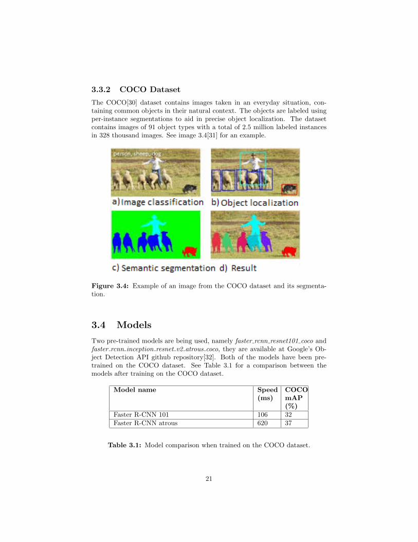
The COCO[30] dataset contains images taken in an everyday situation, con-taining common objects in their natural context. The objects are labeled usingper-instance segmentations to aid in precise object localization. The datasetcontains images of 91 object types with a total of 2.5 million labeled instancesin 328 thousand images. See image 3.4[31] for an example.

Figure 3.4: Example of an image from the COCO dataset and its segmenta-tion.

3.4 Models

Two pre-trained models are being used, namely faster rcnn resnet101 coco andfaster rcnn inception resnet v2 atrous coco, they are available at Google’s Ob-ject Detection API github repository[32]. Both of the models have been pre-trained on the COCO dataset. See Table 3.1 for a comparison between themodels after training on the COCO dataset.

Model name Speed(ms)

COCOmAP(%)

Faster R-CNN 101 106 32Faster R-CNN atrous 620 37

Table 3.1: Model comparison when trained on the COCO dataset.

21

In the table, the speed variable is the model’s speed which is reported in mil-liseconds per 600x600 image and the lower this number is the better. Thesenumbers depend highly on hardware, these specific numbers were generatedwith the model running on a Nvidia GeForce GTX TITAN X graphics card.The COCO mAP (mean Average Precision) variable refers to the models abilityto classify an object, where the higher number is better.

From the table we can derive that model Faster R-CNN 101 is ∼6 times fasterbut at a cost of its accuracy when compared to the Faster R-CNN atrous model.

3.5 Evaluation

The evaluation of the models is done by first collecting 100 images of the parkinglot at different times of the day with the parking lot containing different amountof cars. The images are then manually looked at to mark the number of cars ineach image. The images are then used by the models and the output looked atto determine how accurately the models were able to predict how many cars thatwere in the images. Other factors, such as missed cars and wrongly predictedobjects are also looked at.

3.6 Raspberry PI

With the idea to do the image processing without saving any images and onlysaving the image processing result, a Raspberry PI model 3 was used. Themodel, after being trained on the laptop which uses an Intel(R) HD Graphics4600, was transferred over to the PI. The plan was to take the PI and its fittingcamera model and place it in a fitting position to watch over the parking lot andthen start the image processing remotely from the laptop. The PI would thentake an image, process it and then send the output to the laptop. The outputcould for example be: 2 out of 10 parking spots were occupied at some specificlocations in the image. Thus, the image is not saved and no other informationis extracted. Unfortunately, running the models on the Raspberry PI resultedin a memory error so the Raspberry PI was eventually abandoned.

22

Chapter 4

Experiments

This section explains the experiments and visualizes how the result of the ex-periments conducted on one image looks like.

The experiments were conducted using five different methods consisting of 100images of an angle from the second floor over a parking lot, see Figure 1.1. Thegoal of the experiments is to recognize all the cars in the images. The images’size vary between two sizes, 400x720 and 530x960. The parking lot in the im-ages consists of ten parking spaces.

The bounding boxes shown in the images represents a prediction, the model’sprediction of a car being in a specific spot can vary between 0-100%. Only theimages with predictions over 40% certainty is shown with the purpose to elim-inate unwanted predictions. The value 40% was chosen by running the modelson a few images to see what a suitable limit would be for the models to predictthe cars.

4.1 Methods

The different methods used to conduct the experiments have different impacton the result, the different methods are listed below.

• Method 1 - Pre-trained models without any additional training and nobox optimization, see Section 4.2 and 4.3.

• Method 2 - Pre-trained models with additional training but no box opti-mization.

• Method 3 - Pre-trained models without any additional training but withbox optimization.

• Method 4 - Pre-trained models with additional training and box optimiza-tion.

23

4.2 Box Optimization

Box optimization is used when two bounding boxes overlap with a certain per-centage, when this phenomena occurs the box with lower accuracy is removed.The experiments were conducted with the overlap percentage limit being 50%.

4.3 Additional Training

The additional training consists of 1000 type 2 images and 500 type 3 imagesfrom the PKLot dataset, see image type description in Section 3.3.1. Differentamount of images and different types of images were used but did not yield agood result until the dataset consisting of 1500 images was used. The modelstrained on the dataset for ∼400 training iterations in order for the error loss tostabilize and level out. The Faster R-CNN 101 model ended its training with anerror loss of ∼0.02 after 4 hours, see Figure 4.1 and the Faster R-CNN atrousmodel ended its training with an error loss of ∼0.08 after 7.5 hours, see Figure4.2.

The lower the total loss, the better the model is, unless the model has over-fitted to the training data. The images were divided into two sets where 10%became the validation set of images and the other 90% became the training set.The loss is calculated from these two sets.

Figure 4.1: Graph showing the total error loss during training of the FasterR-CNN 101 model.

24

Figure 4.2: Graph showing the total error loss during training of the FasterR-CNN atrous model.

4.4 Method 1

See Figure 4.3 for an example of the first image comparison between the twomodels without additional training and no box optimization.

Figure 4.3: Object detection with the models without additional training,Faster R-CNN 101 model(left) and Faster R-CNN atrous model(right).

As visible in Figure 4.3 there are four cars parked on the parking lot. Both ofthe models are able to detect all the cars in the parking lot. The Faster R-CNN101 model is less accurate in its predictions in comparison to the Faster R-CNNatrous model. The reason as to why it says N/A in the image is because the

25

pre-trained label image map is missing, the COCO dataset which the modelswere pre-trained on consists of 91 different objects where cars were one of them.This means that the different colors on the detection boxes in the image referto different objects.

4.5 Method 2

See Figure 4.4 for a comparison of the result of the models with additionaltraining on one of the images. In the figure it is visible that both of the modelsare still able to detect all of the cars in the image. The Faster R-CNN 101 modelhas increased its prediction accuracy a lot compared to when the model had noadditional training while the result of Faster R-CNN atrous remains around thesame as it was before. Both of the models are now trained to detect the carobject and as seen in the figure, this object is predicted with a green boundingbox with its fitting label.

Figure 4.4: Object detection with the models with additional training, FasterR-CNN 101 model(left) and Faster R-CNN atrous model(right).

4.6 Method 3

In this experiment the number of predictions have been reduced between Figure4.5 and Figure 4.3 where no box optimization was used.

26

Figure 4.5: Object detection with the models without additional training butwith box optimization, Faster R-CNN 101 model(left) and Faster R-CNN atrousmodel(right).

4.7 Method 4

In Figure 4.6 there is one prediction for each car, as opposed to Figure 4.4 whereno box optimization was used and one more prediction is visible in the image.

Figure 4.6: Object detection with the models with additional training andwith box optimization, Faster R-CNN 101 model(left) and Faster R-CNN atrousmodel(right).

27

Chapter 5

Result

This section presents the result of the experiments. The combined numberof cars in the 100 images are 539. The data from the experiments is presentedbelow, see Tables 5.1 and 5.2. Predictions is how many cars the model predictedthere to be in the 100 images. Missed cars is how many cars the model havefailed to predict. Wrongly predicted objects is how many other objects that isnot a car but was still a prediction, for example a fence or a door.

Faster R-CNN atrous Predictions Missedcars

Wronglypredictedobjects

Runtime(s)

Method 1 580 33 28 5016.5Method 2 743 5 5 5783.5Method 3 530 33 21 4737.3Method 4 515 26 2 5783.4

Table 5.1: Result of the experiment of the Faster R-CNN atrous using 100images.

Faster R-CNN 101 Predictions Missedcars

Wronglypredictedobjects

Runtime(s)

Method 1 568 68 33 1487.9Method 2 612 103 3 2495.8Method 3 508 70 33 1478Method 4 434 107 2 2604.8

Table 5.2: Result of the experiment of the Faster R-CNN 101 using 100 images.

28

The Faster R-CNN atrous model is expected to have a better result consideringthe difference in accuracy between the models but is also expected to be slower,see Table 3.1 in Section 3.4. The following subsections analyzes the result ofthe models with respect to the different methods used.

5.1 Method 1

In method 1, with no box optimization and no additional training, Faster R-CNN atrous made 580 predictions as opposed to 568 by Faster R-CNN 101, seeFigure 5.1. The total number of predictions made should ideally be 539, sincethere are a total of 539 cars in the 100 images. Both models are doing quite wellregarding the number of predictions, what is more important is the number ofmissed cars which is quite high. The goal is to diminish the amount of missedcars and wrongly predicted objects.

Figure 5.1: Result of method 1.

29

5.2 Method 2

Using method 2, no box optimization but with additional training, the modelsshould be better at predicting cars. This seems to be true, but only for theFaster R-CNN atrous model which only missed 5 cars while Faster R-CNN 101missed 103, see Figure 5.2. The number of predictions are higher for bothmodels as well, considering the number of missed cars got reduced for FasterR-CNN atrous and its number of predictions increased means that there are alot of overlapping predictions.

Figure 5.2: Result of method 2.

5.3 Method 3

In method 3, with box optimization but no additional training, the amount ofpredictions should be lower for both of the models. This seems to be the casesince the models now have the number of predictions at 530 and 508, see Figure5.3, as opposed to 580 and 568, in Figure 5.1.

30

Figure 5.3: Result of method 3.

5.4 Method 4

Method 4, with box optimization and additional training, is expected to be themethod which yields the best result. But, as visible in Figure 5.4 both of themodels are quite far away from having 0 missed cars. The amount of wronglypredicted objects is at it lowest across all the methods which is good. It seemsthat the box optimization has removed too many overlapping predictions whichis why the number of missed cars for the Faster R-CNN atrous model has goneup to 26 from its lowest at 5 in Figure 5.4.

31

Figure 5.4: Result of method 4.

5.5 Summary of Results

It is safe to say that the Faster R-CNN atrous model improved a lot with addi-tional training but that adding box optimization increased the number of missedcars. The Faster R-CNN 101 model did surprisingly not benefit from any addi-tional training nor box optimization.

If one were to choose between the different models the obvious choice wouldbe the Faster R-CNN atrous model since the training did not work out forFaster R-CNN 101. But an important note is that the Faster R-CNN atrousmodel was ∼2.5 slower when processing 100 images.

See Figure A.1, A.2 and A.3 in Appendix A for a visual representation of themeasuring parameters between the different methods for each model.

32

5.6 Extra Experiment

Since method 4 did not yield the expected result and ended up performingworse than method 2, where no box optimization was used, another experimentwas conducted with method 4 together with the Faster R-CNN atrous modelwith different overlap percentage limits. Instead of only measuring the result ofremoving additional boxes that overlapped with a percentage of 50%, the modelwas run with the following values as well: 60%, 70%, 80% and 90%. See Figure5.5.

Figure 5.5: Box optimization with different overlap percentage limits on theFaster R-CNN atrous model.

As the overlap percentage increases, the amount of predictions increases whichis expected. The important thing to notice is that the number of missed cars isdecreasing as well. This results in a trade-off between the number of predictionsand the amount of missed cars. The amount of wrongly predicted objects isalso increasing slightly, but not a whole lot.

33

Chapter 6

Discussion

This section discusses the reasons behind the result and proposes ideas to im-prove said result. Other topics, such as how companies use this technology aswell as other areas for neural networks are also discussed.

6.1 Reasons for Unsatisfying Result

There can be a lot of different reasons as to why a model did not yield a satisfyingresult.

6.1.1 Training

One of the reasons could be bad training, a lot different parameters can betuned to achieve different result. One of the parameters could have been thelearning parameter, if this parameter is too high it prevents the model fromfinding a minima in the gradient descent algorithm. This does not seem to bethe issue since the error loss displayed in Figure 4.1 is slowly converging to asmall number. This is only one of many reasons as to why the Faster R-CNN101 model received a worse result with additional training. The training couldalso have been too short or that the dataset was not optimal for the model.

6.1.2 Prediction

When the model does a prediction it is set to keep the predictions with anaccuracy of 40%, this value could be increased or decreased in hope to predictmore cars. Changing this value could also cause the model to do more faultypredictions.

6.1.3 Overfitting

One very possible reason could be overfitting. This is because, as mentionedin Section 4.3, the error loss is slowly converging. This means the model is

34

effectively learning and becoming better at predicting cars. But, when the FasterR-CNN 101 model is shown the other images of a completely new parking lot,it performed way worse than it did without additional training.

6.1.4 Dataset

A problem with the dataset used was that only the cars that were parked werelabeled and not other cars driving around inside the parking lot, this meansthat the model would be trained that a car that is not parked is not of interestand will therefore not be a prediction. This scenario is visible in Figure 3.2.

The dataset was collected and created in Brazil, where snowy parking lots arenot something they had to consider. This is why they could focus on what a carin a parking lot looks like in difference to a parking lot in Sweden, where theparking lots could be covered with snow. Because of this, it can be difficult torecognize a parking lot with its separate spaces. Instead, the idea was whetherthe prediction of a car is possible and then determine if it is parked based onits location in the image.

6.1.5 Models

The models used in this thesis are only 2 out of 19 models currently availablein Google’s object detection repository, by using another model the result couldpossibly improve.

6.2 Determining Occupied Parking Spaces

When the models make their predictions, a prediction’s location is accessible.To determine whether or not a car is in a parking space there are different meth-ods one could use. The most desirable solution would be that the system is ableto determine where the parking spaces in the image are located and then simplycompare the parking spaces’ location with the location of the predictions. But,determining what a parking space is and being able to predict a parking space ismore difficult than just predicting cars and is therefore not handled in this thesis.

Another solution would be to simply mark the parking spaces in the imageand compare those to the locations of the car predictions. Why this is notconsidered a desirable solution is because someone would have to go throughthe image and mark out the different locations of the parking spaces, while thisprocess itself can lead to errors, the whole process would have to be redone incase the camera moved the slightest. This being the simpler solution, a simpleGUI was created in Java where the user could create an NxM matrix which rep-resented the parking lot. The user could then enter the locations of the parkingspaces, and when satisfied press an update button which would start the image

35

processing and produce a result of the vacancy of the parking lot. See Figure6.1 for an example.

Figure 6.1: The image used for the image processing with the predicted cars(left), and the result presented where the red spaces are occupied spots, thegreen spaces are empty spots and the white spaces are unavailable spots (right).

6.3 Other Areas for Neural Networks

There are many other areas where neural networks are being used such as videogames, voice recognition and more.

Video Games Google’s DeepMind[33] uses a deep learning technique referredto as deep reinforcement learning. Researches used this method to teach acomputer to play the Atari game Breakout.

Voice Generation and Recognition Google’s WaveNet[34] is a deep learn-ing network that generates a voice automatically. The system learns to mimichuman voices by themselves and improve over time.

Environment Issues Computers can process a lot more data than humansand because of this, a system using this type of technology should be able toprocess big amounts of different data linked to the environment and recognizepatterns within the data and from these patterns come up with effective solu-tions.

Autonomous Cars Using this technique, cars will eventually become au-tonomous by recognizing different threats in traffic and reading traffic signs toabide traffic laws.

36

6.4 How Companies use CNNs

Data. Companies that have a substantial amount of data are more likely tohave an advantage over their competitors. The more training data available,the more training iterations are possible. This means more weight updates arepossible which in turn forms a better tuned network.

37

Chapter 7

Conclusion

While there are other models that might perform better, the models used inthis thesis are able to detect cars to some extent in the experiments. In orderto use the models in an application applied to a real system, the result shouldbe 0 missed cars which either model managed to do but the Faster R-CNNatrous model was very close with only 5 missed cars. Faster R-CNN atrous isas expected not as fast as Faster R-CNN 101 but is way more accurate whichis more important in a situation like this. As mentioned earlier, the RaspberryPI could unfortunately not be used for the image processing using this approach.

Back to the original question: Can this functionally be delivered using state-of-the-art technology? The answer is yes, the result of the experiments is notoptimal but it is a good result. By changing the training, tweaking the differentparameters, trying out different models and using a larger, different and morediverse dataset; it is possible to detect all cars in a parking lot and determinethe parking lot’s vacancy.

38

References

[1] Express.co.uk. (2017). PARKING NIGHTMARE: You won’t believe the amount of timedrivers spend looking for a space. [online] Available at: https://www.express.co.uk/life-style/cars/827333/Car-park-drivers-looking-for-spaces-cities-research [Accessed 6 Jun.2018].

[2] En.wikipedia.org. (1957). Frank Rosenblatt. [online] Available at:https://en.wikipedia.org/wiki/Frank Rosenblatt [Accessed 6 Jun. 2018].

[3] Perceptron. (2013). [image] Available at:https://blog.dbrgn.ch/images/2013/3/26/perceptron.png [Accessed 6 Jun. 2018].

[4] Convolutional Neural Network. (2015). [image] Available at:https://upload.wikimedia.org/wikipedia/commons/6/63/Typical cnn.png [Accessed6 Jun. 2018].

[5] Corgis. (n.d.). [image] Available at:https://c1.staticflickr.com/7/6098/6365026845 bbc3166923 b.jpg [Accessed 6 Jun. 2018].

[6] A Beginner’s Guide To Understanding Convolutional Neural Networks. (2016). [Blog]Available at: https://adeshpande3.github.io/adeshpande3.github.io/A-Beginner’s-Guide-To-Understanding-Convolutional-Neural-Networks/ [Accessed 6 Jun. 2018].

[7] A Beginner’s Guide To Understanding Convolutional Neural Networks Part 2.(2016). [Blog] Available at: https://adeshpande3.github.io/adeshpande3.github.io/A-Beginner’s-Guide-To-Understanding-Convolutional-Neural-Networks-Part-2/ [Accessed6 Jun. 2018].

[8] Nielsen, M. (2015). Convolution. [image] Available at:http://neuralnetworksanddeeplearning.com/images/tikz44.png [Accessed 6 Jun. 2018].

[9] Outline of dog. (2006). [image] Available at:https://upload.wikimedia.org/wikipedia/commons/thumb/a/ac/Heraldiquechien courrent.svg/800px-Heraldique chien courrent.svg.png [Accessed 6 Jun. 2018].

[10] Nair, V. and E. Hinton, G. (2010). Rectified Linear Units Improve RestrictedBoltzmann Machines. [article] Toronto: University of Toronto, pp.1-8. Available at:http://www.cs.toronto.edu/∼fritz/absps/reluICML.pdf [Accessed 6 Jun. 2018].

[11] Max pooling. (2015). [image] Available at:https://upload.wikimedia.org/wikipedia/commons/e/e9/Max pooling.png [Accessed 6Jun. 2018].

[12] Srivastava, N., Hinton, G., Krizhevsky, A., Sutskever, I. and Salakhut-dinov, R. (2014). Dropout: A Simple Way to Prevent Neural Networksfrom Overfitting. [article] Toronto: University of Toronto. Available at:https://www.cs.toronto.edu/∼hinton/absps/JMLRdropout.pdf [Accessed 6 Jun.2018].

[13] Ruder, S. (2017). An overview of gradient descent optimization algorithms. [article]Dublin: NUI Galway. Available at: https://arxiv.org/pdf/1609.04747.pdf [Accessed 6Jun. 2018].

39

[14] Gradient descent. (2004). [image] Available at:https://upload.wikimedia.org/wikipedia/commons/7/79/Gradient descent.png [Ac-cessed 6 Jun. 2018].

[15] Xu, J. (2017). Deep Learning for Object Detection: A Comprehensive Review. [Blog]https://towardsdatascience.com. Available at: https://towardsdatascience.com/deep-learning-for-object-detection-a-comprehensive-review-73930816d8d9 [Accessed 6 Jun.2018].

[16] Girshick, R., Donahue, J., Darrell, T. and Malik, J. (2014). Rich feature hierarchiesfor accurate object detection and semantic segmentation Tech report. 5th ed. [article]Berkeley: UC Berkely. Available at: https://arxiv.org/pdf/1311.2524v5.pdf [Accessed 6Jun. 2018].

[17] Girshick, R., Donahue, J., Darrell, T. and Malik, J. (2014). R-CNN. [image] Availableat: https://arxiv.org/pdf/1311.2524v5.pdf [Accessed 6 Jun. 2018].

[18] Cortes, C. and Vapnik, V. (1995). Support-vector networks.20th ed. [article] Holmdel, NJ: ATT Bell Labs. Available at:https://link.springer.com/article/10.1007%2FBF00994018 [Accessed 6 Jun. 2018].

[19] En.wikipedia.org. (n.d.). Linear regression. [online] Available at:https://en.wikipedia.org/wiki/Linear regression [Accessed 6 Jun. 2018].

[20] Girshick, R. (2015). Fast R-CNN. 2nd ed. [article] Microsoft Research. Available at:https://arxiv.org/pdf/1504.08083.pdf [Accessed 6 Jun. 2018].

[21] Girshick, R. (2015). Fast R-CNN. [image] Available at:https://arxiv.org/pdf/1504.08083.pdf [Accessed 6 Jun. 2018].

[22] Yang, J. (2017). ReLU and Softmax Activation Functions. [Blog] https://github.com.Available at: https://github.com/Kulbear/deep-learning-nano-foundation/wiki/ReLU-and-Softmax-Activation-Functions [Accessed 6 Jun. 2018].

[23] Ren, S., He, K., Girshick, R. and Sun, J. (2016). 3rd ed. [article] Available at:https://arxiv.org/pdf/1506.01497.pdf [Accessed 6 Jun. 2018].

[24] Ren, S., He, K., Girshick, R. and Sun, J. (2016). Region Proposal Network. [image]Available at: https://arxiv.org/pdf/1506.01497.pdf [Accessed 6 Jun. 2018].

[25] Ren, S., He, K., Girshick, R. and Sun, J. (2016). Faster R-CNN. [image] Available at:https://arxiv.org/pdf/1506.01497.pdf [Accessed 6 Jun. 2018].

[26] Research.google.com. (n.d.). Google Brain Team. [online] Available at:https://research.google.com/teams/brain/ [Accessed 6 Jun. 2018].

[27] GitHub. (2017). Tensorflow Object Detection API. [online] Available at:https://github.com/tensorflow/models/tree/master/research/object detection [Ac-cessed 6 Jun. 2018].

[28] R.L. de Almeida, P., S. Oliveira, L., S. Britto Jr, A., J. Silva Jr, E. and L. Koerich, A.(2015). PKLot – A robust dataset for parking lot classification. [article] University ofParana. Available at: http://www.inf.ufpr.br/lesoliveira/download/ESWA2015.pdf [Ac-cessed 6 Jun. 2018].

[29] R.L. de Almeida, P., S. Oliveira, L., S. Britto Jr, A., J. SilvaJr, E. and L. Koerich, A. (2015). Parking lot. [image] Available at:http://www.inf.ufpr.br/lesoliveira/download/ESWA2015.pdf [Accessed 6 Jun. 2018].

[30] Lin, T., Maire, M., Belongie, S., Bourdev, L., Girshick, R., Hays, J., Perona, P., Ra-manan, D., Zitnick, C. and Dollar, P. (2015). https://arxiv.org/pdf/1405.0312.pdf. 3rded. [article] Microsoft. Available at: https://arxiv.org/pdf/1405.0312.pdf [Accessed 6Jun. 2018].

[31] Lin, T., Maire, M., Belongie, S., Bourdev, L., Girshick, R., Hays, J., Perona, P., Ra-manan, D., Zitnick, C. and Dollar, P. (2015). COCO dataset image segmentation. [image]Available at: https://arxiv.org/pdf/1405.0312.pdf [Accessed 6 Jun. 2018].

40

[32] GitHub. (2016). Tensorflow detection model zoo. [online] Available at:https://github.com/tensorflow/models/blob/master/research/objec detection/g3doc/detection model zoo.md [Accessed 6 Jun. 2018].

[33] DeepMind. (n.d.). DeepMind. [online] Available at: https://deepmind.com/ [Accessed 6Jun. 2018].

[34] DeepMind. (2016). WaveNet: A Generative Model for Raw Audio — DeepMind.[online] Available at: https://deepmind.com/blog/wavenet-generative-model-raw-audio/[Accessed 6 Jun. 2018].

41

Appendix A

Additional Graphs from theResult

Figure A.1: Result of the predictions between the different methods and mod-els.

42

Figure A.2: Result of the missed cars between the different methods andmodels.

Figure A.3: Result of the wrongly predicted objects between the differentmethods and models.

43