COUNTING FOR RIGIDITY, FLEXIBILITY ANDEXTENSIONS VIA THE PEBBLE GAME ALGORITHM

ADNAN SLJOKA

A THESIS SUBMITTED TO THE FACULTY OF GRADUATE STUDIES

IN PARTIAL FULFILLMENT OF THE REQUIREMENTS

FOR THE DEGREE OF

MASTER OF SCIENCE

GRADUATE PROGRAM IN MATHEMATICS AND STATISTICS

YORK UNIVERSITY,

TORONTO, ONTARIO

SEPTEMBER 2006

COUNTING FOR RIGIDITY, FLEXIBILITY AND EXTENSIONS VIA

THE PEBBLE GAME ALGORITHM

by Adnan Sljoka

a thesis submitted to the Faculty of Graduate Studies of York University in partial

fulfillment of the requirements for the degree of

MASTER OF SCIENCE

c© 2006

Permission has been granted to: a) YORK UNIVERSITY LIBRARIES to lend or sell

copies of this thesis in paper, microform or electronic formats, and b) LIBRARY AND

ARCHIVES CANADA to reproduce, lend, distribute, or sell copies of this thesis any-

where in the world in microform, paper or electronic formats and to authorize or pro-

cure the reproduction, loan, distribution or sale of copies of this thesis anywhere in the

world in microform, paper or electronic formats.

The author reserves other publication rights, and neither the thesis nor extensive

extracts from it may be printed or otherwise reproduced without the authors written

permission.

ii

..........

iii

Abstract

In rigidity theory, specifically combinatorial rigidity, one can simply count vertices

and edges (constraints) in a graph to determine the rigidity and flexibility of a corre-

sponding framework. The 6|V | − 6 counting condition for 3D, through the molecular

conjecture by Tay and Whiteley, and a fast ‘pebble game’ algorithm which tracks

the underlying count in the multigraph, have led to the development of the program

FIRST, which analyzes the rigidity and flexibility of proteins in a matter of seconds.

Starting with a detailed description of the 6|V | − 6 pebble game algorithm we

illustrate the algorithm on sample multigraphs. We further extend the pebble game

algorithm to quantify the relative degrees of freedom of a specified region (core) in the

multigraph and identify the regions that are relevant as constraints with respect to

the core. We derive and prove several key pebble game invariants of these extended

algorithms. These new extensions (algorithms) can be used to study important bi-

ological applications, such as hinge motions between protein domains, allostery and

for speeding up simulations in a program such as FRODA.

iv

To my parents

v

Acknowledgments

With a deep and sincere sense of gratitude, I would like to express many thanks to

my supervisor, Professor Walter J. Whiteley. Without his assistance and invaluable

guidance, the work in this thesis would have been impossible. Through his remarkable

vision and enthusiasm for exploration of new ideas, Prof. Whiteley has taught me a

lot about research, how to ask the important questions, come up with useful examples

and formulate conjectures. He provided a motivating and critical atmosphere during

the discussions we had. The company and assurance from Professor Whiteley at

the time of crisis would always be remembered. Professor Whiteley offered many

suggestion on this thesis, he was always there when I need his advice.

I extend an enthusiastic thank you to Professor Jorg Grigull for his interest

and conversations about this thesis.

I would also like to thank all the instructors from the Canadian Bioinformatics

Workshops, from whom I have learned a lot. Further thanks goes to Don Jacobs and

other participants at the workshop in Tempe, for fruitful discussions.

I would also like to express my appreciation to a good friend and graduate

student, Naveen Vaidya, for his support, advice and valuable conversations. Thanks

also goes to Alexandr Bezginov for developing an external FIRST interface, which

allowed me to test out my method with a few proteins, and who is currently working

on further implementations.

vi

I would like to thank my parents for their love and continued support. They

were always there for me. Thanks also goes to my brother for his encouragement. I

would also like to express many thanks to Louisa for her love and understanding.

vii

Contents

Abstract . . . . . . . . . . . . . . . . . . . . . . . . . . . . . . . . . . . . . . iv

Acknowledgments . . . . . . . . . . . . . . . . . . . . . . . . . . . . . . . . vi

List of Figures . . . . . . . . . . . . . . . . . . . . . . . . . . . . . . . . . . x

1 Introduction . . . . . . . . . . . . . . . . . . . . . . . . . . . . . . . . . . 1

1.1 Outline and Motivation . . . . . . . . . . . . . . . . . . . . . . . . . . 1

1.1.1 Protein flexibility is an important phenomenon . . . . . . . . 2

1.1.2 Protein flexibility can be studied using Rigidity Theory . . . . 4

1.1.3 Work Outline . . . . . . . . . . . . . . . . . . . . . . . . . . . 8

2 Rigidity Theory: Searching for the Counts . . . . . . . . . . . . . . 11

2.1 History . . . . . . . . . . . . . . . . . . . . . . . . . . . . . . . . . . . 11

2.2 Bar and joint frameworks . . . . . . . . . . . . . . . . . . . . . . . . 12

2.2.1 Definitions, Rigidity and Infinitesimal Rigidity . . . . . . . . . 17

2.3 Counting and Rigidity of Graphs . . . . . . . . . . . . . . . . . . . . 26

2.4 Counting is not sufficient in 3-dimensions . . . . . . . . . . . . . . . . 33

3 Other Counts and The Pebble Game Algorithm . . . . . . . . . . . 37

3.1 Body-Bar, Body-Hinge . . . . . . . . . . . . . . . . . . . . . . . . . . 38

3.2 The Pebble Game Algorithm . . . . . . . . . . . . . . . . . . . . . . . 48

3.2.1 Illustration of the Pebble Game Algorithm and other analysis 56

3.2.2 Useful Properties of the Pebble Game Algorithm . . . . . . . . 66

4 Problems . . . . . . . . . . . . . . . . . . . . . . . . . . . . . . . . . . . . 71

4.1 Description of the problems . . . . . . . . . . . . . . . . . . . . . . . 72

4.2 Methods and solutions . . . . . . . . . . . . . . . . . . . . . . . . . . 78

viii

4.2.1 Solution - First Problem . . . . . . . . . . . . . . . . . . . . . 78

4.2.2 Illustration of Drawing Back Maximum Free Pebbles . . . . . 82

4.2.3 Solution - Second Problem . . . . . . . . . . . . . . . . . . . . 82

4.3 Examples of finding relevant regions . . . . . . . . . . . . . . . . . . . 91

4.4 Ambiguity . . . . . . . . . . . . . . . . . . . . . . . . . . . . . . . . . 97

5 Verifying the Algorithms Solve the Problems . . . . . . . . . . . . . 111

5.1 Properties - First Problem . . . . . . . . . . . . . . . . . . . . . . . . 112

5.1.1 Greedy Characteristic of the Pebble Game Algorithm . . . . . 113

5.1.2 Matroid . . . . . . . . . . . . . . . . . . . . . . . . . . . . . . 115

5.2 More key pebble properties . . . . . . . . . . . . . . . . . . . . . . . . 118

5.2.1 G has no redundant edges . . . . . . . . . . . . . . . . . . . . 118

5.2.2 G with stress: Exchange as a pebble process . . . . . . . . . . 123

5.3 Properties - Second Problem . . . . . . . . . . . . . . . . . . . . . . . 136

6 Conclusion . . . . . . . . . . . . . . . . . . . . . . . . . . . . . . . . . . . 140

6.1 Applications and Future Work . . . . . . . . . . . . . . . . . . . . . . 141

6.1.1 Identifying degrees of freedom in a hinge . . . . . . . . . . . . 141

6.1.2 Allosteric interactions . . . . . . . . . . . . . . . . . . . . . . 150

6.1.3 Other applications . . . . . . . . . . . . . . . . . . . . . . . . 157

6.2 Concluding remarks . . . . . . . . . . . . . . . . . . . . . . . . . . . . 158

Appendix A Pebble Game Algorithm in 2D for 2|V | − 3 count . . . . 161

References . . . . . . . . . . . . . . . . . . . . . . . . . . . . . . . . . . . . . 168

ix

List of Figures

1.1 FIRST output for HIV protease (PDB id: 1hhp) in a an open (ligand-

free) form) showing rigid region decomposition. The flaps are impor-

tant to the function of this protein, and are determined to be flexible

(indicated by red, yellow and green bonds, each colour indicating a

rigid microcluster within a flexible region). The rest of the protein is

dominated by a single rigid region (coloured in blue). Adapted from [11]. 7

2.1 Rectangle is an example of a flexible bar and joint framework as it

deforms into a parallelogram, altering the distance between the diago-

nals (a). Adding an extra bar (in the place of a diagonal) makes this

framework rigid (b), as the distances between all pairs of joints will

remain fixed. The addition of an extra bar to a rigid framework (c) is

unnecessary (redundant) and the framework becomes stressed. . . . . 16

2.2 Infinitesimal edge condition. The length of each edge in the framework

stays the same to the first order. . . . . . . . . . . . . . . . . . . . . . 20

2.3 Graph of a tetrahedron, a K4 graph. . . . . . . . . . . . . . . . . . . . 22

2.4 Example of a nongeneric (degenerate) case. This framework is rigid

but not infinitesimally rigid (rank is less than maximum rank). These

cases are extremely rare, and here it occurs because of the special

geometry (top three vertices are on a line). . . . . . . . . . . . . . . . 25

x

2.5 Well-distributed (independent) edges is an important concept. Both

graphs have the required minimum number of edge, 2(6) - 3 = 9 edges,

but because the edges in graph (a) are not well-distributed (the sub-

graph induced by the top four vertices has more edges than required,

2(4) - 3 = 5 edges are required, but it has 6 edges, which means that

one edge is wasted (redundant)), so this graph is flexible. On the

other hand, the graph in (b) is minimally rigid as all the edges are

well-distributed (independent). . . . . . . . . . . . . . . . . . . . . . . 29

2.6 Using Laman’s Theorem for 2-dimensional graphs. The graph in (a) is

minimally rigid as it satisfies the conditions from Laman’s Theorem.

The graph in (b) is rigid and stressed. In (c) we see an example of

a graph that has the minimum required number of edges for rigidity,

but some edges are redundant (indicated in blue). This graph is flex-

ible and stressed. The graph in (d) is flexible, it has less than eleven

edges. This example clearly illustrates that flexibility in the graph (in

2-dimensions) occurs for two reasons, either the edges are not well-

distributed, or there are too few edges in the graph. . . . . . . . . . . 31

2.7 A rigid graph with no triangles. . . . . . . . . . . . . . . . . . . . . . 32

2.8 An example which shows that Laman type of counts are not sufficient

in 3-dimensions. This graph, which is known as the double banana,

has 18 well-distributed edges, but it is still flexible. . . . . . . . . . . 35

3.1 Body-bar structure. Two rigid bodies, each having six degrees of free-

dom are connected by a series of five bars (a) (adapted from [11]). In

(b), let us consider the two shaded triangles as rigid bodies. Connect-

ing these two bodies by six bars (indicated by thick black lines) will

rigidify (lock) the two bodies together, so that the structure remains

with only six ever-present trivial degrees of freedom (motions of a rigid

body). This structure can also be viewed to be an octahedron as a bar

and joint framework, which is also known to be rigid [56]. . . . . . . . 39

xi

3.2 Body-hinge becomes the multigraph (body-bar). In (a) we have two

(fully rigid) bodies, which are joined by a hinge (highlighted in bold),

the bodies maintain the contacts at the hinge. The hinge removes five

degrees of freedom leaving a total of seven degrees of freedom (or one

internal (non-trivial) degree of freedom – rotation around the hinge).

The body-hinge can be thought of as a special case of the body-bar,

when the hinge is replaced by five bars (edges) (b). In replacing each

hinge by five edges, we get a multigraph, two vertices (bodies) and

five edges in this case (c). Once the graph of the body-hinge structure

is transformed into a multigraph, the 6|V | - 6 count is used to check

rigidity/flexibility. . . . . . . . . . . . . . . . . . . . . . . . . . . . . . 44

3.3 Example of a minimally rigid (isostatic) multigraph (a). All edges are

independent (i.e. well-distributed). In (b) we have shown that this

multigraph decomposes into six edge-disjoint spanning trees, where

each spanning trees is represented by a colour. . . . . . . . . . . . . . 48

3.4 Pebble game algorithm. Place six pebbles on each vertex of the multi-

graph (b). Edges that are covered by the pebble are independent (in-

dicated as an arrow on the edge). The edge that is currently being

tested is highlighted in red. If ends have more than six free pebbles,

from either end we place the pebble on the edge, orienting the edge

accordingly (shown by an arrow) (d). We continue to test and cover

edges one by one, (e) (f) and (g). Free pebbles are being removed as

edges are declared independent, (rigidifying the graph). In (h) we do

not have enough pebbles on the ends. . . . . . . . . . . . . . . . . . . 57

3.5 Pebble game algorithm ... continued. A seventh free pebble is found

and swapped back, and inserted (i, j and k). In (l) we again look for

the seventh free pebble, the free pebble is located further out in the

directed multigraph. Using the cascade (two swaps) along the path

(turquoise), changing the orientation of the full path in the process,

the free pebble appears (m and n), and the edge is successfully covered

(o). . . . . . . . . . . . . . . . . . . . . . . . . . . . . . . . . . . . . . 58

xii

3.6 Pebble game algorithm ... continued. We continue to redistribute the

free pebbles on the graph so that the ends of the edge being tested

have at least seven pebbles. The remaining edges are successfully cov-

ered by pebbles. All edges in this graph are independent (there is no

stress), and having only six remaining free pebbles (6 degrees of free-

dom - trivial motions of a rigid body) indicates that this multigraph is

minimally rigid. . . . . . . . . . . . . . . . . . . . . . . . . . . . . . . 59

3.7 Pebble game algorithm. As usual, six pebbles are placed on each ver-

tex. Testing edges one by one, all edges so far are successfully covered

by the pebble (c). Testing the remaining edge (red), it currently needs

an extra free pebble on its ends (d). Searching in the directed graph

generated by the pebble game, away from this edge, the seventh free

pebble could not be found (e). The edge is declared redundant (indi-

cated by the dashed line) and is not covered by the pebble (f). The

failed search identifies a rigid region (blue vertices and its induced sub-

graph). Notice that this rigid subgraph (or a ring of size five) contains

6|V ′| − 6 (6(5) − 6 = 24) independent (pebbled) edges. The graph is

flexible overall as there are nine free pebbles (three non-trivial (inter-

nal) degrees of freedom). . . . . . . . . . . . . . . . . . . . . . . . . . 62

xiii

4.1 Motivating the notion of relevant and irrelevant. Here we give some

simple examples and our foreseeing of relevant and irrelevant sets. Blue

bodies and black edges represent the core Gc, and green bodies and red

edges represent the part of multigraph G which is tested for relevance

and irrelevance. When the two regions are disconnected in the gen-

eral graph G, a change in rigidity of one region cannot transmit the

information to the other region (I). If the two regions of Gc are con-

nected by a long chain (path of length 9 here) (II), we expect that

the chain will be irrelevant (once we recover the maximum number of

free pebbles back to Gc, no pebbles from Gc would be used to cover

any edge on the chain). On the other hand, we expect a short chain

(path of length 2 here) to be relevant (it will permanently draw some

pebbles from Gc, and hence decrease the number of free pebbles on

Gc). Gc can be considered as a single region (IV). We anticipate that

the dangling end (IV a) is not drawing off any pebbles from Gc, so it

is irrelevant), whereas the short loop (IV b) will be relevant. Based on

these speculations, the core and the short loop (Gc + b) will be merged

to form a larger relevant region. . . . . . . . . . . . . . . . . . . . . . 77

4.2 Outline of two problems. Since the pebble game is a greedy algorithm,

playing on core Gc first and then on the rest of the multigraph will not

make any difference (steps 2 and 3). In the actual algorithm (given

below) this restriction will not be used. Step 5 tells us that some

vertices and edges outside of the Gc will be relevant if there is at least

one arrow (outgoing edge) pointing away from Gc, and if there are

no outgoing edges from Gc then nothing outside Gc is relevant (no

region outside the core is restricting the motion of the core). This

is a simple outline and will be revised later, but it demonstrates the

intuitive relationship between the two problems. . . . . . . . . . . . . 79

4.3 Example of drawing back free pebbles to the core Gc. In (I) the multi-

graph G is given, and in (II) the predefined core Gc is coloured with blue

vertices and black edges, where the rest of the graph is distinguished by

red edges and green vertices. A completed play of the pebble game on

G is shown in (III). The entire graph has eight free pebbles (2 internal

degrees of freedom) and one redundant bond (indicated by the dashed

line). Currently, Gc has only 5 free pebbles. . . . . . . . . . . . . . . 83

xiv

4.4 Drawing back ... Continued. The yellow vertices (vc ∈ Gc) are incident

with outgoing edges out of the core (indicated by red arrows), currently

there are four outgoing edges (IV). We search for a free pebble from

any outgoing edge (never searching over Gc). The pebble is located

and recovered back to Gc along the directed path (which is coloured in

turquoise) (V, VI). The orientation of this path becomes reversed. . . 84

4.5 Drawing back ... Continued. Two more pebbles are recovered back to

Gc using the paths indicated in turquoise (VII, VIII). At this point

we are left with one more outgoing edge out of Gc (IX). This time the

search for a free pebble out of the core leads to a (capped) failed search

(turquoise) as no free pebbles are found. The core Gc now has seven

free pebbles (Problem 1) and one outgoing edge. Note that there is

also one free pebble outside of Gc (on the bottom left vertex), but no

directed path from the core can access this pebble. . . . . . . . . . . 85

4.6 Relevant region decomposition. Given the multigraph G, and some core

Gc (blue) (a subregion within the multigraph G) (I) which could be

predefined by the user. Using the Algorithm 4.2.3, we can identify the

relevant region outside the core, and expand the core to an enlarged

relevant region GR (II). The remaining part of G (coloured in green)

is irrelevant with respect to the core Gc. The entire graph G is now

decomposed into two regions, those that are relevant to the core and

those that are irrelevant with respect to the core. . . . . . . . . . . . 89

4.7 Finding the relevant region with respect to Gc (ring of eight) (which

was defined in Figure 4.3 (II)). There is one outgoing edge (red) from

the core Gc. We find the reachability region (three dark blue vertices)

of the vertex (yellow) incident with the outgoing edge (II). This gives

the relevant region outside the core (enclosed region in (II)), which is

incorporated into Gc (III). Rest of the multigraph is irrelevant. . . . . 92

xv

4.8 Partitioning G into relevant and irrelevant regions with respect to Gc.

The core is defined by blue vertices and black edges connecting them

(I). The pebble game is played on entire multigraph G and free pebbles

are recovered back to Gc (II). There is one redundant edge (indicated

by the dashed line), the rest of the edges are independent (pebbled).

Once the maximum free pebbles are recovered back to Gc, we search

from a vertex (yellow) incident with an outgoing edge (red arrow) and

obtain an enlarged relevant region GR (III and Figure 4.9 IV). . . . . 94

4.9 Partitioning G into relevant and irrelevant regions ... Continued. The

multigraph G is partitioned into relevant (Gc + short loop) and irrel-

evant (dangling end) regions. . . . . . . . . . . . . . . . . . . . . . . . 95

4.10 Relevant and irrelevant between two regions of the core. The core Gc

(blue vertices and black edges) is shown (I). The pebble game is played

on G and the pebbles are recovered back to Gc (II). The core subregion

on the left has one redundant edge (dashed line) and the subregion on

the right has four redundant edges. The (capped) failed search from

Gc gives the relevant region (III). . . . . . . . . . . . . . . . . . . . . 96

4.11 Relevant and irrelevant between two regions of the core ... Continued.

G is partitioned into relevant and irrelevant regions. The bottom con-

nection is irrelevant as we never get a failed (capped) search over these

edges. . . . . . . . . . . . . . . . . . . . . . . . . . . . . . . . . . . . 97

4.12 Finding the relevant region of the core Gc. The core is made of three

disjoint subgraphs, namely R1, R2 and R3 (blue vertices and black

edges). We are testing the “Y” connection between these regions for

relevance. . . . . . . . . . . . . . . . . . . . . . . . . . . . . . . . . . 98

4.13 Finding the relevant region of the core Gc .... Continued. The pebble

game is played on the entire multigraph G and maximum pebbles are

recovered to Gc. The dashed lines indicate redundant edges (edges that

could not be covered by a pebble). . . . . . . . . . . . . . . . . . . . 99

4.14 Finding the relevant region of the core Gc .... Continued. There is

an edge directed out of R2 (indicated by the red arrow). Searching

away from R2 leads to a (capped) failed search and the relevant region

(enclosed region). . . . . . . . . . . . . . . . . . . . . . . . . . . . . . 100

xvi

4.15 Finding the relevant region of the core Gc .... Continued. We finally

obtain the enlarged relevant region GR. The irrelevant region is shown,

and note if we remove (prune) the irrelevant region, GR would become

a disconnected multigraph, that is R1 would become disconnected from

R2 and R3 . . . . . . . . . . . . . . . . . . . . . . . . . . . . . . . . 101

4.16 Ambiguity in finding relevant regions. This example illustrates that

ambiguity may come up with different plays of the pebble game. In

(I) the core is predefined and clearly distinguished from the rest of

the multigraph G (red edges and green vertices). We performed two

different plays on G, play A and play B, and recovered the maximum

number of free pebbles back to Gc (II). The (capped) failed search

(turquoise path) out of the core in play B shows that the rest of the

multigraph is relevant, meanwhile in play A it is irrelevant, as the

output of play A has no outgoing edges out of Gc (III). . . . . . . . . 103

4.17 Ambiguity in finding relevant regions ... Continued. The enlarged

relevant regions GR are shown for both plays A and B, and are clearly

not unique. . . . . . . . . . . . . . . . . . . . . . . . . . . . . . . . . 104

4.18 Given the multigraph G and the predifined core Gc (blue vertices and

black edges) (I). We play the pebble game on G, and recover the max-

imum number of pebbles to Gc (II). Since there are no outgoing edges

from Gc, there is no relevant region outside of Gc. But, the whole

multigraph is minimally rigid (there are exactly six free pebbles and

no redundant edges). . . . . . . . . . . . . . . . . . . . . . . . . . . . 107

4.19 . The core Gc is defined as the two top vertices, and is enlarged so

it visually stands out (I). The three ‘connections’ between the core

are being tested for relevance. We begin in the usual way, assigning

six pebbles to each vertex (body) in the multigraph. Upon playing

the pebble game algorithm and reversing the maximum number of

free pebbles back to the core (six in this case) (II), we find that any

two of the three connections could come up as relevant (III). This

property is inherent in the rigidity of this multigraph and not in the

pebble game algorithm or the method (Algorithm 4.2.3) we use to find

relevant/irrelevant with respect to the core. . . . . . . . . . . . . . . 110

xvii

5.1 Two different plays on the same graph. Dashed line is the redundant

edge as declared by the pebble game. Both A and B have the same

number of free pebbles (eight free pebbles). The edge that is declared

redundant is different for plays A and B. The distribution of free peb-

bles (i.e. where the free pebbles are located) is also different for the

two outputs. . . . . . . . . . . . . . . . . . . . . . . . . . . . . . . . . 114

5.2 We have recovered g(S) free pebbles to the region S, and 6 of these free

pebbles we drawn to vertex v. The remaining g(S) − 6 free pebbles

are on the other vertices in S (a). We can add g(S) − 6 new edges

(i.e. pebbling these edges) to S connecting all the vertices holding

the free pebble(s) to vertex v. We did not have to use any pebble

draws (cascades) here, we are simply placing pebbles on edges. We

can always do this since v and these other vertices S have at least

seven free pebbles before the edge(s) is inserted. . . . . . . . . . . . . 121

5.3 Two different outputs of the pebble game on the same graph. Dashed

line is the redundant edge. We will not make a distinction between

the two multigraphs, as all pairs of vertices have the same number of

pebbled edges, so no exchange is sought here. . . . . . . . . . . . . . 125

5.4 Exchange-pebble process. Once we have identified the edge we want to

insert (i.e. e ∈ E(B) and e /∈ E(A)), we recover six pebbles to one of

its endvertices (v in this case) (I). Since e is declared redundant in play

A, when we look for the seventh free pebble we will locate some failed

search region RF (II). RF will have at least one edge which is not in

E(B), call it edge f (III). We release the pebble from edge f , place it

back on the appropriate endvertex of f (IV), and draw (reverse) it back

to w along the existing path in RF (i.e. along path S, note that this

path is entirely within the failed search region RF ) (V). We can finally

cover (pebble) the edge e; we have successfully exchanged edges e and

edge f (VI). As we have removed edge f , it has become a redundant

edge. See discussion for when is the exchange-pebble process a valid

part of the pebble game. . . . . . . . . . . . . . . . . . . . . . . . . . 127

5.5 Recovering the pebbles to their original vertices after the exchange.

This is the case where some of the pebbles on v were drawn from

outside of RF , see proof of Lemma 5.2.6 for details. . . . . . . . . . . 132

xviii

5.6 Example of an exchange-pebble process. Given the outputs of the pebble

game A and B on the multigraph G (a ring of size 3) (I). Twelve pebbled

(independent) edges (6(3)-6 = 12) are not equally distributed between A

and B, so we seek to perform an exchange. For instance, we see that the

number of pebbled edges between v and w in A is 2 while in B it is 4; that is

|E(A)vw| = 2 and |E(B)vw| = 4. The goal is to modify the output of A using

exchange(s) so that the number of pebbled edges among all pairs of vertices

u, v, and w is the same as in B. So, we perform the exchange-pebble process

on A, while B is treated as a reference graph and will remain unchanged.

Each time we do an exchange, we get closer to achieving this goal, in this

example two exchanges will be needed. Since B has four independent edges

between v and w, and A has only two independent edges, we let any one

of the redundant edges (not pebbled, indicated by a dashed line) between

v and w in A be the edge we want to insert to A, call it edge e (II). We

draw six pebbles to an endvertex of e (i.e. v) (III). From w we search for

the seventh free pebble, and since we cannot find the seventh free pebble we

locate a failed search (IV). We find edge f in the failed search, release its

pebble and return it to u (V). The free pebble on u is recovered (swapped)

back to w (VI). Now that we have seven free pebbles on the ends of e, we

can pebble the edge e (VII), hence, we have successfully exchanged edges

e and f (we get A(1)). Another exchange is required (since |E(A(1))vw| 6=|E(B)vw|). Continued in the next figure ... . . . . . . . . . . . . . . . . . 134

5.7 Example of an exchange-pebble process ... Continued. We seek another

exchange. Details are not show, the process is the same as in the previous

figure. The two edges (e and f) that will be used in this exchange-pebble

process are shown (VIII). Upon completing the second and final exchange

(obtaining A(2)), all pairs of vertices have the same number of pebbled edges

as in the reference graph, play B (IX), that is |E(A(2))vw| = |E(B)vw|. . . 135

xix

6.1 Extracting degrees of freedom for the hinge. In (a) we are given two

rigid regions R1 and R2. In terms of the pebble game each gets six

free pebbles. In (b) we see that the hinge connecting R1 and R2 has

removed six free pebbles, rigidifying R1 and R2 into a single rigid body,

so this is a hinge of zero (internal) degrees of freedom. In (c) we have

a hinge with one (internal) degree of freedom, as we are able to recover

only seven free pebbles to R1 and R2. In (d) and (e) we have a hinge

with two and three degrees of freedom. The example in (f) illustrates

that even if there is a connection (like a long flexible tether here), we

can recover all 12 free pebbles to R1 and R2 as is the case in (a) where

there is no connection between R1 and R2. . . . . . . . . . . . . . . . 147

6.2 Extracting the number of degrees of freedom for the hinge between two

rigid regions using FIRST. Rigid cluster decomposition of the im-

munoglobulin (PDB code: 1igt) from FIRST is shown (a). Regions

that are identical in colour belong to a same region. The gray (or

black) regions are mostly flexible. In (b) we highlight the Fab arm

region, which consists of two large rigid regions (coloured in blue and

brown) and the flexible region (a tether coloured in gray), more com-

monly known as the ‘elbow’. In (c) we have isolated the two rigid

regions by deselecting everything else in PYMOL, and labeled them

R1 and R2. In (d) we have added five edges (bars) (in the appropri-

ate file that FIRST processes) between the two rigid regions and ran

FIRST again. This rigidified the two regions into a single larger rigid

region (indicated in blue). Since we had to add five edges (less than

5 was not sufficient) indicates that this hinge (‘elbow’) region has five

degrees of freedom. . . . . . . . . . . . . . . . . . . . . . . . . . . . . 149

xx

6.3 A schematic representation of the two types of allostery. On the left

we have a positive regulation, where the binding of a ligand on site A

(a(ii)), causes a conformational change on another distant site B on

this protein (a(iii)), so that site B is now more likely to recognize and

bind its ligand (a(iv)). The transmission from one site to another is

indicated as a wavy yellow arrow. On the right side of the diagram we

have another type of allosteric interaction called negative regulation. A

ligand in only bound on site B (b(i)). When the site A binds a ligand

(b(ii)) this causes the shape of site B to be modified (b(iii)), which

induces the release of the ligand at site B (b(iv)). . . . . . . . . . . . 153

6.4 Finding relevant and irrelevant region can be used to predict allostery.

Here, we apply Algorithm 4.2.3 and find the relevant region with respect to

the core Gc (R1 and R2) (a). The relevant region of R1 and R2 is shown

in (b), and the enlarged relevant region GR (which includes R1 and R2) is

given in (c). There is an allosteric transition between R1 and R2. When

R1 becomes less flexible, R2 also becomes less flexible. That is if we add

an edge to R1, pebbling this edge will cause R2 to loose one free pebble.

Also, if we remove one of the edges from R1 (make it more flexible), this

will cause R2 to also become more flexible, as we could recover an extra free

pebble to R2. So, a change in the degree of freedom (free pebbles) on R1,

that is to say a change in rigidity, will cause a change in degree of freedom

on R2. Furthermore, this allosteric transition, or coupled communication,

between R1 and R2 could only be transmitted over the relevant region, and

not in the irrelevant region. . . . . . . . . . . . . . . . . . . . . . . . . 156

A.1 2|V | − 3 pebble game algorithm. We want to test the graph in (a) for

rigidity/flexibility. We start by placing two pebbles on each vertex

(b). We test edges one by one. The edge that is currently tested is

highlighted in red. If we have four free pebbles on the ends of the edge,

we can pebble that edge (i.e. that edge is declared independent), and

we direct that edge. . . . . . . . . . . . . . . . . . . . . . . . . . . . . 165

xxi

A.2 2|V | − 3 pebble game algorithm ... Continued. In (j) the edge that is

being tested has only three free pebbles on its ends. We perform a swap

with the neighbouring edge (j) and the fourth free pebble appears, and

we can now pebble that edge (l). We continue to test and pebble more

edges (m). In (n) the edge being tested (in red) has only one free

pebble on its ends, so we recover two more free pebbles (o) - (r). . . . 166

A.3 2|V | − 3 pebble game algorithm ... Continued. As we cannot recover

the fourth free pebble, the last edge is declared redundant (indicated

as a dashed line) (u). The graph is flexible as it has four remaining

free pebbles. . . . . . . . . . . . . . . . . . . . . . . . . . . . . . . . . 167

xxii

Chapter 1

Introduction

1.1 Outline and Motivation

Proteins (from the Greek “protos” meaning “of primary importance”) are the most

versatile macromolecules in all living organisms and perform crucial functions in es-

sentially all biological processes. These macromolecules function as catalysts, they

transport and store other molecules such as oxygen, they provide mechanical support

and immune protection, they generate movement, transmit nerve impulses, among

many other biologically significant tasks [4]. Proteins are involved in all kinds of

molecular interactions: with other proteins, DNA, RNA, and small molecules (drugs).

Proteins are composed of sequences drawn from twenty amino acids, also known as

the building blocks of life, and each protein has its own specific sequence of amino

acids (primary structure). We can think of the twenty amino acids as an alphabet,

and the sequence of these amino acids (up to hundreds of letters in length) gives words

(proteins), and thousands of different words with different meanings makes a rich and

powerful biological language. This linear sequence of amino acids (alphabet) com-

pletely defines the 3-dimensional shape or structure of the protein (protein folding).

It would be ideal to have a computer program, which takes an amino acid sequence

1

of a particular protein and deduces or predicts its 3-dimensional structure (specific

spatial positions of atoms). In spite of considerable efforts, the protein folding prob-

lem remains one of the most basic intellectual challenges in molecular biology [4].

Protein structures are extremely important as they are directly related to their spe-

cific function, and often it is possible to guess how a protein works by looking at its

structure.

Fortunately, protein structures can be determined (at atomic resolution) by

experimental methods such as x-ray crystallography or nuclear magnetic resonance

(NMR) techniques. Like all experimental techniques, these methods have their lim-

itations, and are not to be taken to be exact. The number of solved structures is

continuing to increase at a rapid rate; the current count from the PDB database (a

protein data bank) is about 34,000 known protein structures [5], of which the major-

ity are solved by x-ray crystallography. This enormous amount of information has

become instrumental in further analysis and understanding of protein structures and

their connection to important biological phenomenon, and general advances in fields

such as Proteomics.

A quick visualization of the protein’s 3-dimensional structure using any popular

molecular visualization software, such as RASMOL or PYMOL [42, 43], reveals their

immense complexity. Proteins typically contain thousands of atoms, and despite

their complexity, they are fairly compact. They commonly form motifs with regular

periodicity, such as alpha helices and beta sheets.

1.1.1 Protein flexibility is an important phenomenon

In their native (folded) state, proteins are not entirely rigid structures, they have

enough stability to maintain their 3-dimensional structure, while retaining some flex-

ibility to perform essential functions. The secondary structural elements (such as

2

alpha helices or beta sheets) of domains as well as entire domains (stable regions)

undergo movements in space, either fluctuations of individual atoms or collective mo-

tions of group of atoms. Following the basic principle: if you know how it moves,

you can infer how it works, the knowledge of protein flexibility offers a straight-line

connection between its structure and function. In addition to understanding the pro-

tein structure, there is a tremendous amount of evidence and ongoing research to

support the importance of protein flexibility and how it relates to function. For ex-

ample, many proteins need the ability to bind and then release a molecular partner,

or ligand, and this requires some internal mobility (intrinsic flexibility). Intrinsic

flexibility in proteins is the ability of different regions in a protein to move relative to

each other with only a small expenditure of energy [13]. Drastic conformational re-

arrangements within some proteins are known to occur during and after ligand (and

drug) binding [27]; this is also illustrated in a coherent manner by the induced fit

model of substrate-protein interaction. Advancing our knowledge about flexible and

rigid regions of the protein can clearly offer insight into its function, but it also be-

comes possible to extensively explore the ensemble of conformations at a given time,

and predict the changes in flexibility with the varying pH and temperature values.

These can all be important tools in the study of protein-protein interactions and in

drug design.

Understanding protein flexibility and its motion is a complex task, and proba-

bly one of the most complicated biological phenomenon that can be studied in great

quantitative detail. Several methods have been suggested with many limitations.

One popular approach is to compare the snapshots of different conformational states

obtained for a protein from an experimental technique, like x-ray crystallography or

NMR spectroscopy. Since these methods were primarily designed to determine the

3

three-dimensional static representation of a molecule, that is the set of {x, y, z} coor-

dinate values for each atom in the protein, they are often very limited in the amount

of information they can offer regarding the protein flexibility. The biggest issue with

this method is the lack of diversity (and accuracy) of the conformational states that

are available for comparison. Only a fraction of 34,000 known protein structures

have multiple conformations [5], and most of them are from NMR experiments which

are limited to small or average size proteins. Another common method attempts to

simulate the protein’s motion, by means of molecular dynamics. A downside of this

method is that it is computationally extremely expensive (especially with larger pro-

teins), as it tries to simulate all possible motions based on the physical laws. It is

particularly not suitable in simulating or probing large-scale conformational changes

that are observed in proteins which are functionally very important, such as the hinge

motions between domains [13], (which occur on the order of microsecond (10−6) to

millisecond (10−3)) scale, whereas each time step in molecular dynamics simulation is

on the femtosecond (10−15) time scale) [30]. The computational time needed to reach

these large scale motions is beyond practical wide-range application.

1.1.2 Protein flexibility can be studied using Rigidity Theory

An elegant and ingenious method was recently developed for studying protein flexi-

bility. This method relies on graph theory and the branch of mathematics called the

rigidity theory (see Chapter 2), and it has resulted in the development of software

program Floppy Inclusion and Rigid Substructure Topography (FIRST) [11] which is

available on the web, and another similar program PROFLEX [33]. In short, FIRST

takes a single static 3-dimensional structure (snapshot) of the protein (i.e. PDB file)

and creates a multi-graph (body-bar graph) where atoms are represented by vertices

4

and edges represent the distance constraints corresponding to the intramolecular in-

teractions of a protein (i.e. covalent bonds, double and peptide bonds, hydrogen

bonds, hydrophobic interactions). Computationally, FIRST uses the pebble game al-

gorithm (arising from the rigidity theory) to do the flexibility analysis (degrees of

freedom counting), and outputs the number of degrees of freedom associated with

the protein, which directly tells us about its rigidity/flexibility. Using the pebble

game algorithm, FIRST also outputs all the rigid and stressed (rigid with extra con-

straints) regions (these terms will be defined later on) and other flexible connections

(corresponding to rotatable bonds) as a rigid cluster decomposition, and can track

the changes in these regions during simulated thermal denaturation, along with other

useful properties. All of this information can be nicely mapped (coloured) back on the

protein and can be viewed with several molecular visualization software. For detailed

explanations see [7, 27, 32].

It is important to note that the flexibility predicted by FIRST corresponds

to a “virtual” (snapshot – infinitesimal) motion as a prelude to real (finite) motion.

FIRST provides static and kinematic information, not dynamic. Only the potential

of motion is identified, but this corresponds to finite motions (for generic cases, see

next chapter). A useful analogy would be as if we are identifying a hinge on a door,

where the motion is known to occur, without actually moving or understanding how

far the door can move (i.e. bumping of atoms is not modeled). This idea of the

snapshot, mathematically better known as “infinitesimal” rigidity, will be discussed

in Chapter 2.

One of the best features of the FIRST is that it is exceptionally fast, where

large proteins can be analyzed in a fraction of a second on a standard processor.

Many proteins have been analyzed using FIRST and the results have been shown

to correlate well with the corresponding experimental evidence [7, 22, 27, 28, 32].

5

FIRST has also been successfully applied on very large molecular structures such as

viral capsids, containing hundreds of proteins [22]. In fact, the original motivation

for the pebble game algorithm was to analyze the rigidity/flexibility of the covalent

glass networks, with millions of atoms [24]. The detailed workings and explanation

of FIRST will not be given here, this can be found in several papers [27, 32] and on

the FLEXWEB (FIRST) server [11]. The pebble game algorithm, the main driving

force behind FIRST is central to this thesis and will be discussed and demonstrated

in detail (Chapter 3).

As a quick demonstration of FIRST and the general importance of studying

protein flexibility, let us look at one particular example. It is well known that having

some flexibility in the binding site (where protein binds to another protein, ligand

or molecule) is an important feature of protein function, and in many instances it

is directly related to design of new drugs [4]. A good example of this is the HIV

protease, which is responsible for viral maturation, and is a major inhibitory drug

target [32, 52]. This protein is a dimer composed of two identical monomers, each

having 99 amino acids, and has been the focus of intensive research in both academic

and pharmaceutical communities. In Figure 1.1 we have shown the output of FIRST

for HIV protease [32] (in open conformation – without ligand). We can see that most

of this protein is composed of a single large rigid region, which is coloured in blue.

The “flaps” (at the top) are determined to be flexible, and this is indicated by the

red and yellow bonds. This flexibility analysis given by FIRST closely matches the

experimental evidence [32].

The flexibility and movement of the flap (loop) regions are very important

and directly related to the function of the HIV protease. The flaps act like chemical

scissors and cleave important polyproteins into individual functional proteins and

enzymes. These individual proteins are necessary for the virus to mature [46]. The

6

Flaps

Figure 1.1: FIRST output for HIV protease (PDB id: 1hhp) in a an open (ligand-free)form) showing rigid region decomposition. The flaps are important to the functionof this protein, and are determined to be flexible (indicated by red, yellow and greenbonds, each colour indicating a rigid microcluster within a flexible region). The restof the protein is dominated by a single rigid region (coloured in blue). Adaptedfrom [11].

7

flexibility of the flaps is necessary as they need to open for the segments of the

polyprotein to access the active site [46]. There have been several drugs (protease

inhibitors) developed which will disable this process. The drug binds at the flaps and

stops them from moving, rendering the protein dysfunctional [52]. As a result, the

virus does not mature and noninfectious viruses are produced. There is also some

evidence that drug-resistant mutations of the protease cause a change in shape and

flexibility in the flap region, and it is thought that this causes resistance (reducing

affinity) to drug binding [46].

Studying protein flexibility is an important and yet complicated biological

phenomenon, and FIRST is proving to be a valuable tool in such an undertaking.

FIRST is a very powerful method, and a completely novel way of studying protein

flexibility, and like most new methods, it still needs some refinements and fine tun-

ing to better match the biology and experimental evidence; this is part of ongoing

research [7, 11, 37].

Protein rigidity/flexibility is the ‘motivating factor’ behind our studies. We

are primarily interested in the mathematical and algorithmic workings of the pebble

game algorithm, which is the main component of FIRST. One of the main goals of this

thesis is to extract and formulate some interesting and applicable problems, which

can be answered in an algorithmic fashion by utilizing the pebble game algorithm.

1.1.3 Work Outline

We will begin by outlining some basic results and definitions from rigidity theory

(Chapter 2). For the sake of simplicity we will start by looking at the most common

and simplest structures known as bar and joint frameworks. Bar and joint frameworks

are a natural starting point in rigidity theory studies, and will sharpen our general

8

understanding. Since the fast algorithms for determining the rigidity/flexibility (luck-

ily) do not rely on the complicated geometry (positions of joints and bar lengths),

we will quickly switch to the combinatorial results of rigidity/flexibility. As we will

see, the combinatorial results are based solely on the underlying connections of the

framework, in other words the rigidity becomes a graph theoretic property, and this

gives fast algorithms (i.e. pebble game) for determining rigidity/flexibility. We will

also briefly present some problems with finding the fast (combinatorial) algorithms

for determining flexibility of the bar and joint frameworks in 3-dimensional space.

Chapter 3 presents a different and unusual type of structure (body-bar, body-

hinge) without all the details. This structure is not commonly studied, but is being

used to model molecules (as it is in FIRST) and surprisingly has nice (combinatorial)

results which also provide fast pebble game algorithms for studying rigidity/flexibility.

We will also present the molecular conjecture, a crucial mathematical tenet connecting

the rigidity results (and the pebble game) to molecules (proteins), which facilitated

the development of FIRST. Because the pebble game is central to our studies, we

will outline the pebble game algorithm for these special structures, describe the basic

pebble operations and give some detailed examples. Since pebble game algorithm

for these special structures is poorly documented in the literature, we believe that

this is an important task. We will also present some basic well-known pebble game

properties, which were recently presented by Lee and Streinu [36].

In Chapters 4 and 5 we will present some of our original work. There are

two main problems that are of concern to us. First, we will use the pebble game

algorithm and outline the method that can be used to quantify the relative degrees

of freedom of any region(s) (core) of the entire graph (protein). The core can be any

biologically significant region (for example a domain or a binding site of the protein).

We will further extend this analysis and identify the relevant and irrelevant regions

9

with respect to some predefined core. In short, the relevant regions are those regions

that affect the rigidity/flexibility (motions) of a core (subgraph), while irrelevant

regions have no affect. This will be properly defined and explained. We will illustrate

several examples of both identifying the relative degrees of freedom and detecting the

relevant and irrelevant regions. Chapter 5 will be mainly devoted to proving some

critical pebble game properties to verify that the algorithmic solutions to our problems

are correct. In Chapter 6 we will give some possible biological applications in terms

of protein flexibility arising from our work, and offer some concluding remarks and

directions for further future work.

10

Chapter 2

Rigidity Theory: Searching for the

Counts

This chapter is devoted to introduce some concepts from rigidity theory, develop

the definitions and useful vocabulary. Only the basic concepts of infinitesimal rigid-

ity (see below) are introduced here, while leaving the details and illustrations to be

found in the references provided. We are mostly interested in the counting results

(section 2.3) of the rigidity and the related discussions. These counting (graph the-

oretical) characterizations of rigidity will be the most important in the subsequent

chapters.

2.1 History

We can trace the roots of the rigidity theory back to Euler (1766) where he conjectured

that “A closed spatial figure allows no changes, as long as it is not ripped apart” [16].

Using today’s terminology, a closed spatial figure is a closed polyhedral surface made

up of rigid polygonal plates that are hinged along the edges where plates meet. La-

grange (1788) introduced the constraints on the motion of mechanical systems, which

11

was again used by Maxwell [39] (1864) and a number of engineers studying the statics

of bar and joint frameworks [32]. Even though rigidity theory has a rich history, it is

only in the last thirty years that it has started to find applications in basic sciences.

The modern era of combinatorial theory starts with the important theorem of Laman

(1970) (see below) which made the combinatorial approach to the subject rigorous in

2-dimensions, and is seen as the foundation for the multiple important applications

arising from rigidity theory (for instance, in sensors and communications, material

science, of course protein flexibility, etc.) [2, 51, 58].

2.2 Bar and joint frameworks

We begin by looking at the most widely studied structure, which is composed of

bars (rods) and joints. The main ideas are first represented qualitatively and later

defined more formally. For simplicity, in this chapter we will strictly look at the

2-dimensional (plane) bar and joint frameworks, unless stated otherwise. Since the

majority of interesting applications are found in 3-space, it is important to note that

almost all of the definitions and concepts in 2-dimensions have natural extensions

and generalizations in 3-dimensional and higher dimensional space (all discussion is

in the Euclidean space). Even though bar and joint frameworks are not currently used

to model proteins (such as FIRST), they serve as a good starting point in order to

introduce the widely-used definitions and vocabulary from rigidity theory, and these

structures are simple enough that we can visually perceive and appreciate most of

the necessary concepts and definitions.

In bar and joint frameworks, the bars (which connect a pair of joints) are

assumed to be perfectly rigid (will not get shorter, longer, or break) and the joints, also

known as universal joints (or ball joints) are completely flexible (free to rotate) [44].

The joints (points in two-dimensional space - explained below) basically serve as a

12

connection between a collection of bars, which only impose the restriction that the

bars share the common endpoints. The bars correspond to fixed distances (act as

distance constraints) between some pairs of joints. Imagine we want to move (in a

continuous manner) such a framework in the plane, consisting of bars connected at

their ends (joints), then the distances between all pairs of joints that are connected by

a bar will remain fixed throughout the motion. The natural and interesting question

that rigidity theory poses is: will the distances between other (non-connected) pairs

of joints also remain fixed?

It is clear that we are interested in understanding the motions of this struc-

ture (framework), as the possible motions will guide us to the answers about rigid-

ity/flexibility of the structure. Informally, we can say that a deformation (or flex,

formal definition given below) is a motion which preserves the lengths of all of the

bars of the framework but changes the distance between some (at least one) pairs of

(unconnected) joints of the framework. If no deformation exists, then the motion is

said to be a rigid motion of a framework. So, a rigid motion of the framework pre-

serves the distance between all joints (points) in the framework, whether the joints

are connected by a bar or not. We can say that a framework is rigid if it has no

deformations (all of its motions are rigid motions), and is flexible otherwise1. Rigid

motions (or rigid body motions) are often referred to as trivial motions, and any other

motions arising from deformations are known as non-trivial motions. We are clearly

interested in motions of a framework that go beyond the ever-present trivial motions,

that is motions other than those from congruences (i.e. translations and rotations).2

1These terms are sometimes differently used in the rigidity theory literature, for instance, flex issometimes synonymously used with motion, whether it is trivial or non-trivial [47, 58].

2We are not considering reflections as we are only interested in continuous motions.

13

There is a widely used concept which talks about the possible motions in terms

of degrees of freedom. The idea of degrees of freedom is used in many different multi-

disciplinary fields (in chemistry, engineering, robotics, ... etc.). Roughly speaking, the

degrees of freedom is the number of parameters needed to describe the position of the

body, say in the plane or in three-space [16]. Here we give the basic intuition. First

of all, consider something as simple as a single point (joint) in the plane. In order to

bring this point to any position in the plane, a horizontal and a vertical translation

are enough (translation in the x and y direction). So, we say that a point in the plane

has ‘two degrees of freedom’ [16]. Another way to think of this is to coordinatize the

plane and see that it takes two real numbers (two pieces of information) to identify

the location of the point (each coordinate changes independently of the other one).

Similarly, in three-space a single point (joint) would have three degrees of freedom

(three numbers to specify its position).

Now, consider two distinct points (joints) P and Q in the plane. If P and Q

are connected by a bar, their distance is fixed. This simple framework will be a rigid

object, but we can still move it using rigid body motions (translations, rotations). P

and Q collectively have four degrees of freedom, and the placement of the bar reduces

this to three degrees of freedom. More specifically, we can bring P to any position

in the plane with vertical and horizontal translation (two degrees of freedom). Then,

if Q is not yet in the requested position a further rotation around P will assure this

(one degree of freedom). So, a single bar has three degrees of freedom, it takes three

pieces of information to specify its position in the plane (two translations, followed

by a rotation). Furthermore, any rigid body in the plane with at least two distinct

points, has three degrees of freedom. Once the position of two points is fixed (which

takes three degrees of freedom), the entire rigid body is fixed (all other points (joints)

will be in the fixed positions) [44].

14

So, any bar and joint framework (with at least two distinct joints) will have

at least three degrees of freedom, corresponding to trivial motions (rigid body mo-

tions). We will sometimes refer to the three ever-present degrees of freedom as the

trivial degrees of freedom. Clearly flexible frameworks in the plane will have more

than three degrees of freedom. Extra degrees of freedom (corresponding to non-trivial

motions) are normally called the internal degrees of freedom [16]. In detecting rigid-

ity/flexibility of a framework, it is of clear interest to know how many internal degrees

of freedom are present. Rigid frameworks have zero internal degrees of freedom.

Most of the discussion in this chapter will be related to bar and joint frame-

works in two-dimensions, but for future clarity, we need to point out that a rigid

structure in three dimensions, with at least three not collinear points (joints) has six

degrees of freedom3. We give the basic reasoning. For any rigid body in three space,

once three of its points (joints) are fixed, the entire body is fixed. Intuitively, three

joints collectively have nine degrees of freedom. The nine degrees of freedom are

reduced to six when the three bars are added forming a triangle. More specifically,

call the three (non-collinear) points in three-space P , Q and R. To move the point P

to any desired position in three-space it takes three degrees of freedom (the combina-

tion of three translations). Relative to P , we can bring Q to a desired position on a

two-dimensional sphere around P [44]. This is a combination of two rotations (think

of longitude and latitude on the globe), and it adds two more degrees of freedom.

Relative to P and Q, a rotation around PQ axis (one degree of freedom) can finally

bring R to the final position, giving a total of six degrees of freedom for any rigid

body in 3-dimensional space [16, 44]. For further details and explanations see [16, 44].

Let us look at a simple example of a bar and joint frameworks in two-dimensions

(plane). From Figure 2.1(a) we can clearly see that a rectangle is a simple example

3It is clear that on the line (1-dimension) that a rigid body has one degree of freedom (it canonly translate along the line)

15

of a flexible bar and joint framework, since it deforms into a parallelogram. The

rectangle has four degrees of freedom, the three trivial degrees of freedom, and one

internal degree of freedom4. The internal degree of freedom corresponds to the extra

motion (deformation) when we fix (hold) the bottom two joints, allowing the top and

two side bars to move. On the other hand, a rectangle with a diagonal (extra bar

present) (in Figure 2.1 (b)) is rigid, it has three degrees of freedom, zero internal

degrees of freedom. We can only move this framework by utilizing the ever-present

trivial motions (translations, rotations), which preserve all the pair-wise distances5.

Adding another diagonal (Figure 2.1 (c)) is clearly unnecessary as the framework is

already rigid (it has no effect on the degrees of freedom). This framework is now

stressed (definition given below).

(a) (b) (c)

Figure 2.1: Rectangle is an example of a flexible bar and joint framework as it deformsinto a parallelogram, altering the distance between the diagonals (a). Adding anextra bar (in the place of a diagonal) makes this framework rigid (b), as the distancesbetween all pairs of joints will remain fixed. The addition of an extra bar to a rigidframework (c) is unnecessary (redundant) and the framework becomes stressed.

4Note that this framework has four joints (eight degrees of freedom - five internal degrees offreedom), and when we place four bars (each bar reduced the degrees of freedom by one), we haveremoved four degrees of freedom, leaving 8 − 4 = 4 degrees of freedom (one internal degree offreedom). This intuitive approach works here, but more sophisticated approach and further analysiswill be need in matching bars (constraints) with degrees of freedom.

5Note that the actual motions of a framework should also take place in the plane, otherwise therectangle with a diagonal bar present can clearly deform if we allow it to fold (a reflection) likea hinge about the diagonal, which makes it flexible in the 3-dimensional space. This is a generalproblem in the sub-field of rigidity theory that deals with global rigidity (rigid in next dimensionalspace), and is of no concern to us.

16

2.2.1 Definitions, Rigidity and Infinitesimal Rigidity

So far we have offered the intuitive discussion of concepts, but to allow for any detailed

study, we need to give precise mathematical definitions and notations. First we state

some basic definitions from graph theory.

A graph G = (V,E) consists of a vertex set V = {1, 2, ..., n} and edge set E,

where E is a collection of unordered pairs of vertices called the edges of the graph (an

edge connects a pair of vertices). We say that two vertices i and j are adjacent if edge

e = {i, j} is present in the graph. The edge {i, j} is said to be incident to vertices i

and j, conversely, the vertices i and j are incident to the edge {i, j}. Sometimes we will

abbreviate the edge e = {i, j} as ij when no confusion can arise (for instance, when

vertices are one digit positive numbers). The vertices i, j are called the endvertices

(or ends) of edge ij. A subgraph of G = (V,E) is a graph G′ = (V ′, E ′), with V ′ ⊆V and E ′ ⊆ E and we simply write G′ ⊆ G. If G′ ⊆ G and G′ contains all edges ij

∈ E with i, j ∈ V ′, then G′ is an induced subgraph of G. Alternatively, the subgraph

induced or spanned by a set of vertices is the graph consisting of those vertices and

all edges that are only incident to those vertices. A loop6 is an edge which joins a

vertex to itself (i.e. e = {i, i}). An edge is multiple if there is another edge with same

endvertices. The multiplicity of an edge is the number of multiple edges sharing the

same endvertices. A multigraph is a graph which contains multiple edges. Graphs

can also be directed, meaning that edges are ordered pairs of vertices (i.e. edges get

a preferred direction, which is usually identified by an arrow on the graph). Other

graph theoretic definitions that we will use in this and subsequent chapters, along

with further explanations can be found in any introductory book to Graph Theory

(for instance [10]).

6Loops (or bridges) are also a common term used in protein structures [4], and are not to beconfused with the graph theoretical meaning.

17

From now on, bars will be represented by edges and joints by vertices. More

formally, we define a 2-dimensional bar and joint framework as a triple (V, E, p)

where G = (V,E) is a simple graph (no loops or multiple edges) and a corresponding

configuration p : V → R2, which assigns each vertex to a point in the plane7. For

simplicity, we will always assume that the endvertices of every edge in the framework

have distinct points (i.e. all edge lengths have positive values). For 3-space, the

definition is the same, except p : V → R3. The framework (V, E, p) is often simply

denoted as G(p). As a convenient abuse of notation we write the point p(i) as pi, i

∈ V , and we usually denote the coordinates of pi (in 2-dimensions) by (xi, yi). It is

also a common and useful approach to denote p as a single point in R2n (n = |V |)(i.e. p = (p1, p2,...,pn)) [16, 56], we will adapt this from now on.

A motion (or finite motion) p(t) of the bar and joint framework G(p) is a family

of smooth functions p(t) = (p1(t), p2(t),...,pn(t)) 8, 0 ≤ t ≤ 1, such that p(0) = p (i.e.

pi(0) = pi for all i), and

|pi(t)− pj(t)| = |pi − pj| = constant, for all {i, j} ∈ E and 0 ≤ t ≤ 1 (2.1)

[16, 20] i.e. Under the motion p(t), the distance (Euclidean) of each edge in the

framework is kept fixed.

A motion p(t) of G(p) is a flex (non-trivial, deformation) if |pi(t) − pj(t)| 6=|pi − pj| for t > 0, and some {i, j} /∈ E (i.e. p(t) is not congruent to p(0) = p for all

t > 0 - distance between some pairs of vertices can vary). A framework is flexible if

it has a flex, and is rigid otherwise (has only trivial (rigid body) motions) [56, 60]9.

That is, for a rigid framework |pi(t) − pj(t)| = |pi − pj| for all i, j ∈ V and t > 0.

7p is sometimes called the embedding function [16].8In the extended form p(t) = (p1(t), p2(t),...,pn(t)) = (x1(t), y1(t), x2(t), y2(t),...,xn(t), yn(t))9We should note that there are several other, equivalent ways in defining a framework to be rigid

and flexible (see [58]).

18

So, in a rigid framework, every motion p(t) will preserve the distances of all pairs of

vertices, whether they are adjacent or not.

We can rewrite equation (2.1) in terms of the usual dot product,

(pi(t)− pj(t)) · (pi(t)− pj(t)) = cij, for all {i, j} ∈ E, (2.2)

where each cij (constant) is a squared length of edge {i, j} (i.e. cij = |pi − pj|2).Solving this system of |E| quadratic equations and 2|V | unknowns imposed by

distance constraints (edges) in the framework is very difficult even for small systems

(few vertices and edges) (see [16, 44]). One successful alternative approach which is

also common to engineers is to not look for a flex (deformation) directly, but simplify

the quadratic algebra to a more manageable linear algebra, deriving a system of linear

equations by looking at the first derivatives of (2.2). We outline the basics here (see

references for further details).

Thinking of t as time and differentiating edge length constraints from (2.2),

dividing by 2 and evaluating at t = 0, we get10

(pi − pj) · (p′i − p′j) = 0, for all {i, j} ∈ E. (2.3)

where p′i represents the unknown instantaneous (virtual) velocity of the point pi.

The set of instantaneous (initial) velocities (one for each vertex) p′ = (p′1, p′2,...,

p′n) which satisfies condition (2.3) is called an infinitesimal motion or first order

motion [16, 56].

Note that we can rewrite equation (2.3) as (pi−pj)· p′i = (pi−pj) · p′j, and see

that (2.3) basically says that the initial velocities of the endvertices of any edge have

equal projections in the direction of the bar (edge), which is depicted in Figure 2.2.

10p′i(t) = ddtpi(t) = ( d

dtxi(t), ddtyi(t)) is a velocity vector of pi.

19

p i

p j

p i ’

p j ’

p i

– p j

Projection of

pj’onto (p

i– p

j)

Projection of

pi’onto (p

i– p

j)

Figure 2.2: Infinitesimal edge condition. The length of each edge in the frameworkstays the same to the first order.

In other words, an infinitesimal motion assigns a velocity vector p′i to each vertex i so

that the length of edges (bars) present in the graph is preserved to the first order. As

usual we want to know if infinitesimal motion preserves the lengths of non-adjacent

(without an edge) pairs of vertices (see below).

Over all edges the constraints from (2.3) give |E| linear equations and 2|V |unknowns representing p′. Rewriting equation (2.3) as: (pi − pj)·p′i + (pj − pi)·p′j =

0, we can represent this homogeneous system of linear equations as a single matrix

equation

RG(p)p′T = 0 (2.4)

where RG(p) is called the rigidity matrix and p′ = (p′1, p′2,..., p′n) (a 2n-dimensional

velocity vector, p′ ∈ R2n).

The rigidity matrix RG(p) has |E| rows (one for each edge) and 2|V | columns11.

For each edge e ∈ E, its corresponding row has only four nonzero entries (remember

this is for two dimensions) corresponding to the difference in the coordinate values

of its two associated incident vertices. The general form of the rigidity matrix looks

11In 3-dimensions the rigidity matrix is an |E| by 3|V | matrix.

20

like [56]:

RG(p) 1 . . . i . . . j . . . n

.... . .

... . . ....

. . ....

{i, j} 0 . . . (pi − pj) . . . (pj − pi) . . . 0

.... . .

... . . ....

. . ....

For example, consider the graph of a tetrahedron in 2-dimensions (complete

graph on four vertices, a K4 graph) (Figure 2.3).

The rigidity matrix for this framework is:

RG(p) v1 v2 v3 v4

{1, 2} (p1 − p2) (p2 − p1) 0 0

{1, 3} (p1 − p3) 0 (p3 − p1) 0

{1, 4} (p1 − p4) 0 0 (p4 − p1)

{2, 3} 0 (p2 − p3) (p3 − p2) 0

{2, 4} 0 (p2 − p4) 0 (p4 − p2)

{3, 4} 0 0 (p3 − p4) (p4 − p3)

In the extended form (where pi = (xi, yi)) this rigidity matrix becomes:

RG(p) vx1 vy

1 vx2 vy

2 vx3 vy

3 vx4 vy

4

{1, 2} (x1 − x2) (y1 − y2) (x2 − x1) (y2 − y1) 0 0 0 0

{1, 3} (x1 − x3) (y1 − y3) 0 0 (x3 − x1) (y3 − y1) 0 0

{1, 4} (x1 − x4) (y1 − y4) 0 0 0 0 (x4 − x1) (y4 − y1)

{2, 3} 0 0 (x2 − x3) (y2 − y3) (x3 − x2) (y3 − y2) 0 0

{2, 4} 0 0 (x2 − x4) (y2 − y4) 0 0 (x4 − x2) (y4 − y2)

{3, 4} 0 0 0 0 (x3 − x4) (y3 − y4) (x4 − x3) (x4 − x3)

So, instead of looking at the regular (finite) motion and dealing with the unde-

sired quadratic algebra, we are interested in understanding the linearized, infinitesimal

21

1 2

3

4

Figure 2.3: Graph of a tetrahedron, a K4 graph.

motions (i.e. solution p′ = (p′1, p′2,..., p′n) of the linear system RG(p)p′T = 0) of the

framework G(p). An infinitesimal motion p′ is called a trivial infinitesimal motion

(or infinitesimal rigid motion) if it has velocities that arise from a congruence [60]

(i.e. translations and rotations)12. If the solution p′ is not trivial then p′ is called an

infinitesimal flex (or infinitesimal deformation)13. We say that G(p) is infinitesimally

flexible if it has an infinitesimal flex, and is infinitesimally rigid otherwise. Infinitesi-

mal (or first order) motions have recently been referred more intuitively as snap-shot

motions (see [60]). As infinitesimal motions of the framework are solutions of the sys-

tem of homogenous linear equations (solution space), they form a vector space. The

dimension of this vector space (solution space) is of clear interest (see below). The

space of trivial infinitesimal motions (in the plane) is of dimension three, generated

for instance by two translations and a rotation around an origin [16, 56, 60].

Infinitesimal rigidity is a natural and extremely useful approximation to rigid-

ity, and their interconnection has been extensively studied [15, 16, 44, 50, 56, 58]. As

12Note that if we consider that no two vertices are identical, and no three vertices lie on a line(i.e. vertices are in general position [16]) then infinitesimal motion (in the plane) p′ is trivial if(pi − pj)·(p′i − p′j) = 0, for all i, j ∈ V (see [16, 56, 58]).

13When only considering general position of vertices then infinitesimal motion is not trivial if(pi − pj)·(p′i − p′j) 6= 0 for some {i, j} /∈ E (see [16, 56, 58])

22

we are ultimately going to rely on another even more useful approach (combinatorial,

see below), we only state the basic and fundamental results here.

Infinitesimal rigidity and specifically the construction of the rigidity matrix is

useful for properly stating some definitions that we will repeatedly use. A set of edges

is said to be independent if their associated rows in the rigidity matrix are linearly

independent [20]. So, if we were to remove an independent edge, the rank of the

rigidity matrix would change (decreases by one). An edge is said to be dependent

or redundant if removing it from the framework the rank of the rigidity matrix is

not altered (i.e. its corresponding row in the rigidity matrix is linearly dependent).

We say that the total degrees of freedom of the framework G(p) is the dimension of

the solution space of RG(p)p′T = 0 (i.e. the dimension of the space of infinitesimal

motions). It is useful to define the internal degrees of freedom of the framework

as the dimension of the space of infinitesimal motions minus the dimension of the

space of trivial motions (trivial degrees of freedom, i.e. unavoidable solutions). In 2-

dimensions, a framework with at least two (distinct) vertices always has three trivial

degrees of freedom. That is, if G(p) has at least two vertices, the internal degrees of

freedom = total degrees of freedom − 3 trivial degrees of freedom. It is clear that for

an infinitesimally rigid framework G(p), internal degrees of freedom = 0.

Since infinitesimal rigidity can be analyzed from the rigidity matrix (i.e. know-

ing the size of the solution space), we can make use of the linear algebra tools. There

is a standard result in the linear algebra for a homogeneous system of linear equations

that connects equations, solutions and variables: dimension of the solution space = #

columns (variables) − # of independent equations (rank). In this context, we state a

well known result that relates the infinitesimal rigidity to simply computing the rank

of the rigidity matrix [15, 16, 20, 44, 50, 56, 58]:

23

Theorem 2.2.1 A 2-dimensional framework G(p), with |V | > 1, is infinitesimally

rigid if and only if the rigidity matrix RG(p) has (maximal) rank = 2|V | − 3.

In a clear sense, edges are serving as constraints on the possible motions of

the framework, and intuitively, this says that we need 2|V | − 3 independent edges to

attain infinitesimal (first order) rigidity (note that three degrees of freedom of a rigid

body are never constrained). We will look at this in the more detail below.

For completeness, the result for the 3-dimensional framework is:

Theorem 2.2.2 A 3-dimensional framework G(p) with |V | > 2, is infinitesimally

rigid if and only if the rigidity matrix RG(p) has (maximal) rank = 3|V | − 6.

This result is nice and unlike the complicated quadratic algebra, we can now

simply compute the rank of the rigidity matrix (for instance by Gaussian elimination)

and get insight into infinitesimal rigidity. Note that any (2-dimensional) infinitesi-

mally rigid framework will have an infinitesimally rigid subframework with exactly

2|V |−3 independent edges (simply discard the redundant edges – edges corresponding

to rows of zeros after row-reduction).

Since we have introduced two types of rigidity, we clearly would like to know

what is the relationship between the regular rigidity (finite motions) and the infinites-

imal rigidity (‘virtual’ – infinitesimal motion). Again, we state the most basic results.

If we have regular flexing (finite deformations) it follows that we have infinites-

imal flexing, and this is a well known result in the rigidity theory [16, 20, 44, 56, 60]:

Theorem 2.2.3 If a framework G(p) is flexible, then G(p) is infinitesimally flexible.

Equivalently (by a contrapositive), if G(p) is infinitesimally rigid then G(p) is rigid.

For some special and extremely rare cases, the infinitesimal rigidity and regular

rigidity are not quite the same (i.e. frameworks behave atypically). For instance, the

framework in Figure 2.4 is rigid (has only trivial rigid body motions), but it is not24

p1

p2

Figure 2.4: Example of a nongeneric (degenerate) case. This framework is rigid butnot infinitesimally rigid (rank is less than maximum rank). These cases are extremelyrare, and here it occurs because of the special geometry (top three vertices are on aline).

infinitesimally rigid (it has an infinitesimal deformation). If we assign a zero vector to

every vertex in the framework, except to vertex p1 we assign a small non-zero velocity

vector (p′1) (indicated by an arrow) perpendicular to the “chain” (top segment), this

infinitesimal motion will not distort any edges in the framework at first order (the

projections of the vector assigned to the endvertices of each edge are zero), but it

will distort the distance (by infinitesimal amount) say between p1 and p2. One might

think of this infinitesimal motion as the vibration of the chain (see [16]).

Fortunately, these degenerate (or singular) cases like the one in Figure 2.4 are

extremely uncommon, and occur because the framework takes some special degenerate

(singular) configuration p (a geometric issue - in Figure 2.4 this occurs because the top

three vertices are collinear). In fact, if we randomly pick the positions of the vertices

of the framework (configuration p), it is probability 0 that the framework will be in

a degenerate configuration [20, 56, 60]. We are more interested what happens for

the generic configurations (not degenerate), which occur for almost all configurations

(with probability 1 when randomly chosen) [60]. Basically, the generic configurations

p are those configurations which achieve the maximum possible rank of the rigidity

matrix on all subgraphs, details can be found in [16, 56, 60].

25

A valuable result due to Gluck(1975) [14] says that for the generic configu-

rations (almost all configurations), the infinitesimal rigidity/flexibility and regular

rigidity/flexibility agree [60]:

Theorem 2.2.4 (Gluck) For a generic configuration p, a framework G(p) is rigid if

and only if G(p) is infinitesimally rigid.

Equivalently, a framework G(p) is flexible if and only if G(p) is infinitesimally flexible.

We are now assured that (for generic cases) tracking infinitesimal rigidity/flexibility

is actually tracking regular rigidity/flexibility (corresponding to finite motions). For

further details on infinitesimal rigidity and examples see [16, 44, 56, 58]. Since we are

only interested in the generic configurations (ignore ‘exceptional’ cases), we can now

confidently drop the prefix “infinitesimal”. In the literature it is common to refer to

these frameworks as “generically rigid” or “generically flexible”. For our purposes,

in the sequel, we will basically refer to frameworks as rigid or flexible, unless we feel

that there is a danger of confusion.

2.3 Counting and Rigidity of Graphs

Gluck’s result is extremely important, it allows us to completely ignore the location of

the vertices and the precise distances of the edges that are present in the framework,

and instead focus on the topological properties of the framework. In another words,

to understand the rigidity/flexibility properties of the framework G(p), we can now

forget the geometry of the framework (configuration p), and concentrate strictly on

the underlying graph G = (V, E): rigidity becomes a combinatorial property. In

this spirit, we can now step back from our discussion about rigidity/flexibility of

frameworks and start talking about the rigidity/flexibility of graphs (graph rigidity

can be taken to be synonymous with generic rigidity).26

Surely, since we are assuming we are only dealing with the generic cases, we

can randomly pick some positions for the vertices, write the corresponding rigidity

matrix and compute the rank, and see if the graph is rigid. If the rank is equal

to 2|V | − 3 (maximum possible rank), then the graph is rigid and if it is less than

2|V | − 3, then it is flexible. Note that if we find that the graph is flexible (rank is

less than maximum), all this is saying is that the graph will deform infinitesimally,

and therefore (due to Gluck’s Theorem) in a finite sense. We are not concerned how

far it will deform (amplitude of motion), this is a different question (geometric issue

- requires modeling collision constraints (tensegrity theory)).

If our system has thousands, even millions of vertices and edges (as in molecules)

computing the rank is computationally impractical and extremely difficult (i.e. too

slow numerically, get round of errors, etc.). Since rigidity (for generic cases) is now

a property of the underlying graph, we would naturally like to have some sort of a

graph theoretical result that tells us when the graph is rigid and when it is flexible.

So, how can we recognize if the graph in 2-dimensions is rigid? What follows is

an argument that will allow us to correctly predict the answer. Most of this already

follows in one form or another from Theorem 2.2.1 in terms of the rank of the rigidity

matrix. The rank of the rigidity matrix properly defines the mathematical framework

within which the problem is well posed, however, computing with the matrix is not

very practical for our purposes. So, we will replace our discussion from the rigidity

matrix and instead offer combinatorial concepts (vocabularies) and translate some

definitions that were stated in terms of the rigidity matrix to pure graph statements

to make them more effective. This will prove to be central when we look at the

algorithmic approach for determining the graph rigidity/flexibility (i.e. the pebble

game algorithm). Moreover, this matches more closely the vocabulary in graph-

rigidity (i.e. combinatorial rigidity) and in algorithmic-rigidity literature.

27

Because edges are constraining the possible movements of vertices, it is clear

that a graph with many edges is more likely to be rigid than the graph with only few

edges. We need keep in mind, that no matter how many edges the graph has, we will

never constrain the three trivial degrees of freedom (motions of a rigid body). We

say that a graph is minimally rigid or isostatic if it is rigid and removing any one of

its edges (but not vertices) makes the graph non-rigid. So, the ultimate question is:

what is the condition for the graph to be minimally (or isostatically) rigid?

Flexibility in the graph occurs due to unconstrained degrees of freedom. Recall,

in 2-dimensions a single vertex has two degrees of freedom, so it is clear that a graph

which has n vertices (n = |V |) has at most 2n degrees of freedom (possible independent

motions) (it has exactly 2n degrees of freedom when no edges are present). Each edge

(constraint) eliminates at most a single degree of freedom14, so in order to eliminate

all the internal degrees of freedom, then one could anticipate that at least 2n−3 edges

are necessary for rigidity in a graph. However, having the required total number of

edges in the graph is clearly not sufficient, as the edges could be crowded between

only a select few vertices, leaving the other vertices unconstrained (see Figure 2.5

(a)). The goal then, is to have 2n − 3 well-distributed edges. That is, in graphs

with 2n − 3 edges, no subgraph on n′ vertices should have more than its fair share

of 2n′ − 3 edges (see Figure 2.5 (b)). This criterion is sometimes called the Laman

condition, due to Laman [34], and the graphs (subgraphs) that satisfy this condition

are known as Laman graphs (subgraphs). If any subgraph G(V ′), where |V ′| = n′,

has more than 2n′ − 3 edges, then some edges are redundant. Non-redundant edges

are independent. We say that a graph is stressed if it has at least one redundant

edge. Removing a redundant edge from the framework does not affect the rigidity

of that framework (degrees of freedom of the graph before and after its removal stay

14This is only true for graphs with generic configurations. For some degenerate cases (which weare not considering) an edge can remove more than a single degree of freedom (see [16]).

28

a) b)

Figure 2.5: Well-distributed (independent) edges is an important concept. Both graphshave the required minimum number of edge, 2(6) - 3 = 9 edges, but because the edgesin graph (a) are not well-distributed (the subgraph induced by the top four verticeshas more edges than required, 2(4) - 3 = 5 edges are required, but it has 6 edges,which means that one edge is wasted (redundant)), so this graph is flexible. On theother hand, the graph in (b) is minimally rigid as all the edges are well-distributed(independent).

the same)15. It is the independent edges (i.e. well-distributed edges) that eliminate

the degrees of freedom from the graph, so the presence of 2n − 3 independent edges

should be sufficient for rigidity. This basic intuition is correct in 2-dimensions and it

is confirmed in the following famous theorem due to Laman (1970) [34]:

Theorem 2.3.1 (Laman) The edges of a graph G = (V, E) are independent in 2-

dimensions if and only if no subgraph G′ = (V ′, E ′) has more than 2n′ − 3 edges (n′

> 1), where n′ = |V ′|.

Corollary 2.3.2 A graph G = (V,E) with 2n − 3 edges (n > 1) is minimally rigid

in 2-dimensions if and only if no subgraph G′ = (V ′, E ′) has more than 2n′−3 edges,

(n′ > 1), where n′ = |V ′|.15Having a series of redundant edges in framework is a familiar idea to engineers who wish to

build frameworks (structures) with extra strength and failure tolerance properties [20]

29

Laman’s Theorem is the key graph theoretical result in the plane that allows

us to completely characterize minimally rigid graphs. Several other equivalent char-

acterizations have since been discovered [20, 58, 56], and some of these play crucial

roles in finding polynomial time algorithms for testing rigidity of graphs (see below).

Laman’s Theorem allows us to test whether the graph is rigid or flexible (generically)

by simply counting the edges and their distribution in the graph (combinatorial prop-

erty). Computing the rank of the rigidity matrix is a significant improvement over the

complicated quadratic algebra, but Laman’s Theorem is clearly even more powerful.

As a historical note, we should point out that even though Laman was the first to

prove this result, this requirement had been stated in the nineteenth century.

Let us consider a few examples which reveal the usefulness of the Laman’s

Theorem. Consider the graphs in Figure 2.6 (graphs on same sets of vertices). All

of the graphs have seven vertices, so in order for the graph to be minimally rigid we

would need a total of eleven (2(7) − 3 = 11) edges, and all of the edges should be

well-distributed. The graph in Figure 2.6 (a) has eleven edges and by inspection we

can see that no subgraph of n′ vertices has more than 2n′ − 3 edges, so, all eleven

edges are independent (well-distributed). Therefore, by Laman’s Theorem this graph

is (minimally) rigid. The graph in Figure 2.6 (b) is rigid, but it is not minimally rigid

(we added an extra edge), it has 12 edges. This graph is also stressed. It is clear that

any graph that is rigid and not minimally rigid is also stressed (there is a presence

of redundant edge), also known as an overconstrained graph. In Figure 2.6 (c) we

have an example of a flexible graph. This graph has eleven edges, but one subgraph

(indicated by blue edges and its endvertices) does not satisfy the Laman count. The

edges in this subgraph are redundant. This graph shows that a flexible graph can be

stressed. Note that redundant edges always belong to some rigid and stressed (i.e.

30

overconstrained) subgraph. Finally, in Figure 2.6 (d) we clearly have a flexible graph,

as it needs another edge.

(a) (b)

(c) (d)

Figure 2.6: Using Laman’s Theorem for 2-dimensional graphs. The graph in (a) isminimally rigid as it satisfies the conditions from Laman’s Theorem. The graph in(b) is rigid and stressed. In (c) we see an example of a graph that has the minimumrequired number of edges for rigidity, but some edges are redundant (indicated inblue). This graph is flexible and stressed. The graph in (d) is flexible, it has lessthan eleven edges. This example clearly illustrates that flexibility in the graph (in2-dimensions) occurs for two reasons, either the edges are not well-distributed, orthere are too few edges in the graph.

Note that triangles are not required for rigidity. There are many graphs that do

not have triangles, and yet they are rigid. One example is the graph of the complete

bipartite graph K3,3 (see [10] for definition) in Figure 2.7 [56]. This graph has the

31

exact count. It has 2(6) − 3 = 9 edges, and as no subgraphs have too many edges,

all edges are independent (well-distributed).

Figure 2.7: A rigid graph with no triangles.

Laman’s Theorem is an elegant and remarkable result, but in its original form

it is obvious that it gives a poor algorithm. It requires counting the number of edges

in every subgraph, of which there are an exponential number [21] (note that in the

examples in Figure 2.6 we basically used a visual inspection to check the counts). For

the sake of simplicity we will often refer to the Laman count in 2-dimensions as the

2|V |−3 count. We would like to have a fast and efficient algorithm that we can check

this count for rigidity.

As we said previously, Laman’s Theorem has several equivalent formulations.

One particular formulation, originally due to Hendrickson [20] is:

Theorem 2.3.3 For a graph G = (V, E) having m edges and n vertices, the following

are equivalent.

(i) The edges of G are independent in 2-dimensions.

(ii) For each edge {i, j} in G, the graph formed by adding three additional edges

{i, j} has no n′ vertex subgraph with more than 2n′ edges.

32

This formulation was initially used by Hendrickson (as a bipartite matching

algorithm) and later revised by Jacobs and Hendrickson [21], and developed into a par-

ticularly intuitive algorithm, the pebble game algorithm. One of the most distinctive

features of the pebble game algorithm is that it is computationally efficient16. Un-

derstanding the pebble game algorithm is crucial to our studies. We are not going to

give the details of the 2-dimensional pebble game algorithm (the paper by Jacobs and

Hendrickson gives the main steps), because we will concentrate on the pebble game

algorithm for another type of a structure: body-bar/body-hinge structure (which is

used to model proteins in FIRST). It is well known that the main process of all the

pebble game algorithms is essentially the same, with some minor modifications. This

new structure (different count) and the detailed outline and description of the pebble

game algorithm is presented in the next chapter.

Basically, the idea behind the pebble game algorithm is to grow a maximal set

of independent edges one at a time by matching them to the degrees of freedom in

the graph (pebbles). A new edge is added if it is determined to be independent of

the existing set. So, for 2-dimensional graphs (bar and joint frameworks), if 2n − 3

independent edges are found, where n is the number of vertices in the graph, then

the graph is rigid. As we will see (section 3.2), the pebble game gives a unique and

visually appealing way to test edges for independence (track the count), and outputs

several key rigidity properties.

2.4 Counting is not sufficient in 3-dimensions

The graph theoretic analysis of rigidity of frameworks in 3-dimensions is complicated,

not fully understood phenomenon. The equivalent restatement of the Laman condi-

tion for (minimal) rigidity of 3-dimensional graphs (of course generic) would say [56]:

16Other methods were developed previously, for instance by Sugihara [48]

33

A graph G = (V, E) is minimally rigid in 3-dimensions (n> 2) if and only if it has

3n − 6 edges and no subgraph G′ = (V ′, E ′) has more than 3n′ − 6 edges, where n′

= |V ′|.Again, this says that we need enough edges for the graph to be rigid, and

all edges should be well-distributed so that there is no packing of too many edges

between a given set of vertices. These counts are clearly necessary for rigidity. Un-

fortunately, for all of the effective results (appeal) that the Laman condition provides

in 2-dimensions (via constraint counting), the 3|V | − 6 count is not sufficient in

3-dimensions. The graph of the “double banana” in Figure 2.8 is the classical coun-

terexample. This graph satisfies the counts; it has the exact required number of edges

and there are no subgraphs having more than 3n′ − 6 edges connecting n′ vertices.

Accordingly, all eighteen edges are “well-distributed”, but this graph is flexible. Each

banana (a rigid subgraph) is made of two tetrahedra glued together along a trian-

gle, and the two bananas are attached at their tips (top and bottom vertices). It

is clear that the two bananas can twist independently around the (imaginary) axis

through their tips. This imaginary axis is called the ‘implied hinge’ [26] (two rigid

subgraphs of the graph rotate around the hinge). It is conjectured that the only

reason the Laman’s counts fail in 3-dimension, is because of the presence of implied

hinges. This is known as the Dress conjecture [59]. While the double banana is the

smallest example where Laman’s condition is insufficient, several other ones have also

been classified [38, 58, 56].

The problem with the example in Figure 2.8 is that its edges are not inde-

pendent in the sense of Theorem 2.2.2. If we picked some randomly chosen points

for vertices, we would see that the rows of the rigidity matrix are linearly dependent

(rank would drop). Expressing this independence graph-theoretically (using counts)

has proved to be an extremely difficult problem. One can also see that the problem

34

Figure 2.8: An example which shows that Laman type of counts are not sufficient in 3-dimensions. This graph, which is known as the double banana, has 18 well-distributededges, but it is still flexible.

35

with the Laman type of a count in 3-dimensions is that it does not work for a single

edge (i.e. when n = 2) [60]. Not only does the Laman type of count fail here, but

there are currently no known polynomial time algorithms for testing rigidity for gen-

eral 3-dimensional graphs [60]. A lot of work and extensive research has been done

on this problem and to date we can only trace some partial results [56, 58] and count-

ing results conjectured for some special classes of graphs (known as bond-bending

graphs) [26].

Finding complete counting characterizations of general graphs in 3-dimensions

(3-dimensional bar and joint frameworks) that are both necessary and sufficient re-

mains one of the big open problems in rigidity theory.

Considering that many interesting applications are found in 3-space, it is very

unfortunate that we do not have nice compatible counts. On the other hand, a surpris-

ing result is that there are nice counting results for another (perhaps more unusual)

type of a structure, which can be used to model molecules, and most importantly

these results (counts) give fast pebble game algorithms (which are used in FIRST

on proteins) for determining crucial rigidity properties. This is the focus of the next

chapter.

36

Chapter 3

Other Counts and The Pebble

Game Algorithm

In the previous chapter we have seen that Laman’s Theorem provides a powerful

counting condition (2|V |−3 count) for (generic) rigidity of 2-dimensional graphs (bar

and joint frameworks), and that these counts do not extend to general graphs in

3-dimensional space.

In this chapter, we introduce a different type of a structure, called the body-bar

structure, and an astonishing result that provides correct counting (combinatorial)

criteria in 3-dimensional space for determining (generic - graph) rigidity/flexibility,

which leads to a corresponding fast pebble game algorithm. We are interested in these

new structures (i.e. their underlying graphs) and their specializations (body/hinge

structures) because these structures (graphs) are used to predict protein rigidity/flexibility

in FIRST. The first section gives the basic results for these different structures. We

draw particular attention to the section on the pebble game algorithm, a few of its

properties and some illustrative examples.

37

3.1 Body-Bar, Body-Hinge

Because of the applications to proteins, our discussion from now on (unlike the pre-

vious Chapter) will be mainly on structures in 3-dimensional space, even though one

can find comparable results (counts) for 2-dimensional structures [40, 56].

We recall that a rigid structure (with at least three vertices) in 3-dimensional

space always has six trivial degrees of freedom (rigid body motions). In 3-dimensional

bar and joint frameworks, the isolated joints (i.e. vertices) are points which have three

degrees of freedom and some pairs of joints are connected by a single bar (edge), which

act as single distance constraints. In contrast, in body-bar frameworks [49, 56, 60]

(which can at first be perceived as an unusual structure) a body, unlike the joint, is

a fully dimensional rigid object. Since each body is a fully rigid object, it has six

degrees of freedom [56]. Some pairs of bodies are then connected by multiple bars

(which act as constraints), rather than being restricted to a single bar, to make a

body-bar framework1 (see [56]).

In Figure 3.1 (a) there is an illustration of two bodies (rigid objects) which are

joined by five bars. We can think of each bar as removing a single degree of freedom,

so having five bars between the two bodies would have a more of a rigidifying effect

than would a constraint, say with two or three bars between the two bodies. If we

want to make the two bodies into a single rigid region (that is, lock the two bodies

with respect to each other), then six bars should be used2 [49, 56]. This makes sense,

since the two bodies have a total of twelve degrees of freedom and six (properly placed)

bars would remove the six non-trivial (internal) degrees of freedom (see Figure 3.1

(b)). If we have a collection of bodies, we would naturally like to know what is the

minimum number of bars needed and how should they be distributed to make the

1The connection site of the body and one of its bars is again taken to be a universal (ball) joint,which has full flexibility [49].

2It is well known by engineers that six bars are needed to make the two bodies rigid [49].

38

(a)

(b)

Figure 3.1: Body-bar structure. Two rigid bodies, each having six degrees of freedomare connected by a series of five bars (a) (adapted from [11]). In (b), let us considerthe two shaded triangles as rigid bodies. Connecting these two bodies by six bars(indicated by thick black lines) will rigidify (lock) the two bodies together, so thatthe structure remains with only six ever-present trivial degrees of freedom (motionsof a rigid body). This structure can also be viewed to be an octahedron as a bar andjoint framework, which is also known to be rigid [56].

39

resulting structure rigid. Since having more than six bars between any two bodies is

unnecessary, for simplicity we can assume that there can be a maximum of six bars

between any pair of bodies.

Before we proceed further we should point out that, as with the general graphs

(not multigraphs) in 2-dimensions (bar and joint frameworks), we are again strictly

interested in the generic behaviour of these structures (generically placed bars [56, 60])

and generic behaviour of other special cases (see below). In other words, we are only

concerned with the underlying connection between bodies and the distribution of bars

(i.e. their graph). If we think of bodies as vertices and bars as edges, the correspond-

ing graph of a body-bar structure will now be a multigraph G = (V, E) (with no

loops), which allows up to six edges between any pair of vertices (bodies). We are

not going to present the rigidity matrices and corresponding definitions (infinitesimal

rigidity) for these structures (and other specializations, see below), these can be found

in [49, 56, 60]). Presenting this is beyond the scope of this thesis (requires projective

geometry, Cayley algebra, etc.) and is not needed for our purposes and for the pebble

game algorithm (see below). We will just state the basic counting (combinatorial)

results that predict (generic) rigidity of the multigraph G, and use these counts to

introduce the appropriate pebble game algorithm.

Intuitively, the more edges (bars) the multigraph has, the more likely that it

will remove more degrees of freedom, but we would naturally like to know what is the

minimum number of edges needed for rigidity and how should they be distributed (to

be well-distributed – independent) between the vertices (bodies). A remarkable result

was given by Tay [49], who was able to show that there is a counting characterization

(i.e. Laman type theorem) of rigidity for the (generic) body-bar structures:

40

Theorem 3.1.1 (Tay’s Theorem) [49] A body-bar structure in 3-dimensions on the

multigraph G = (V, E) is minimally rigid if and only if it has 6|V | − 6 edges and for

every nonempty subset E ′ ⊆ E with vertices V ′, |E ′| ≤ 6|V ′| − 6.

Considering that counts (Laman type of theorem) do not work for general

graphs (bar and joint frameworks) in 3-dimensions (see graph of ‘double banana’,

Figure 2.8), Tay’s Theorem may seem a bit surprising. It assures us that no ‘double

banana’ (or any other) type of problems can occur here. We will call the count from

Tay’s Theorem, a 6|V | − 6 count. Just as the 2|V | − 3 count (Laman’s Theorem)

completely captures rigidity for general graphs in 2-dimensions, we can use the 6|V |−6

count to test for rigidity of the multigraph G. The criterion |E ′| ≤ 6|V ′| − 6 ensures

that all edges are independent (well-distributed – no subgraph has too many edges).

By this count we can say that the edges in the multigraph G are indepen-

dent if and only if on all the subgraphs on V ′ vertices they satisfy the count |E ′|≤ 6|V ′| − 6. If some subgraph has more than 6|V ′| − 6 edges, then the multigraph

(on this subgraph) will have redundant (dependent) edges and the multigraph will be

stressed. Remember that an independent edge affects rigidity/flexibility (i.e. remov-

ing (adding) it will increase (decrease) the degrees of freedom), while a redundant

edge is not required as it has no effect on rigidity/flexibility (removing or adding it

will leave the same degrees of freedom). In this sense, all of the definitions and dis-

cussions and vocabularies on the general graphs (using 2|V |− 3 count) from previous

chapter naturally generalize here for multigraphs (6|V | − 6 count).

We can clearly see that a multigraph G = (V,E) is rigid, but not minimally

rigid (it has more than 6|V |− 6 edges, i.e. it is rigid and stressed) if and only if there

is a subset |E ′| = 6|V | − 6, and for all non-empty subsets E ′′ ⊆ E ′, |E ′′| ≤ 6|V ′′| − 6.

That is, a rigid multigraph will have a subset of |E ′| = 6|V |− 6 independent edges (a

rigid multigraph has a maximal independent set of edges). We should point out that

41

Tay’s Theorem actually extends for higher dimensional spaces [49, 56], but for our

purposes the 3-dimensional characterization is the most significant. As a side note,

it is important to be aware (as discussed in the previous chapter), that counts are

predicting the infinitesimal (snapshot) motions, but because we are only interested

in the generic behaviour, this matches up with regular motions [60].

We also have a well-know, and useful combinatorial property of the multigraph

G, that connects these counts to the trees in the graph. A tree is a connected graph

on a set of vertices with no cycles of edges (a minimally connected graph) (see in-

troductory book on graph theory for details, for instance [10]). A spanning tree of

a graph G is a subgraph which is a tree and contains all vertices of G [10]. The

following is a special case of a general theorem of Tutte.

Theorem 3.1.2 (Tutte) [53] A multigraph G = (V,E) with 6|V | − 6 edges, satisfies

the count |E ′| ≤ 6|V ′| − 6 on all subgraphs if and only if graph G is a union of six

edge-disjoint spanning trees.

In this spirit, Tay’s Theorem could have been restated in terms of trees3; this

is used in some studies [36], roughly it would say: a multigraph G in 3-dimensions is

minimally rigid if and only if it is a union of six edge-disjoint spanning trees.

Generic body-bar frameworks are usually too general for most built struc-

tures. Another more interesting structure is the body-hinge structure, which can be

considered as a special case of the body-bar structures, with several useful appli-

cations [56, 57]. In this structure, the bodies (vertices), are still fully rigid objects

(have six degrees of freedom), of which some pairs are connected by a (linear) hinge

(lines) [57], where a hinge removes five degrees of freedom between the two bodies.

So for two bodies linked along a hinge, that leaves a total of seven degrees of freedom

3We can write 6|V | − 6 = 6(|V | − 1), and see why we are talking about six spanning trees here.Each spanning tree has |V | − 1 edges [10]. That is, we can think of the |V | − 1 count as the countof a tree.

42

(6 trivial degrees of freedom of a rigid body, and one non-trivial (internal) degree of

freedom – rotation of two bodies around the hinge). When the bodies move, they pre-

serve the contacts at hinges (hinges constrain the movement of two bodies in 3-space)

(see Figure 3.2 (a)).

The underlying graph of the body-hinge structure is now a general (simple)

graph GH = (V, H) (no multiple edges or loops), where V is the set of bodies and

H is the set of hinges (edges). It is useful and logically correct to assume that any

two bodies can be connected with at most a single hinge (edge), since having two

or more (distinct) hinges between two bodies will just lock the two respective bodies

into a single larger rigid unit (see [56]), which might as well be called a single (rigid)

body. This is the reason why the graph GH = (V, H) of the body-hinge structure is

a general graph and not a multigraph.

However, since each hinge removes five degrees of freedom, a useful extension of

the body-hinge structures is to model each hinge as a series of five bars (independent

edges – each independent edge removes a single degree of freedom), and in doing this

we transform GH into a multigraph (see Figure 3.2 (b)). In this spirit, the body-hinge

structure becomes a special case of the body-bar structure. There are some geometric

details in carefully choosing the five bars so that they act as a hinge between the two

bodies (five bars should all pass through the line of the hinge [56]), but again these

geometric details are not important for our purposes. The important consequence for

us is that these structures again have nice combinatorial (counting) properties that

can be used to check rigidity/flexibility. This is confirmed by the following result of

Tay and Whiteley (1984) [56, 57, 58]:

Theorem 3.1.3 (Tay and Whiteley) A body-hinge structure on a graph GH = (V, H)

is rigid (generically) if and only if, each edge (i.e. each hinge) of the graph is replaced

43

by 5 edges, the resulting multigraph contains six edge-disjoint spanning trees on the

vertices V .

(a) (b) (c)

Figure 3.2: Body-hinge becomes the multigraph (body-bar). In (a) we have two (fullyrigid) bodies, which are joined by a hinge (highlighted in bold), the bodies maintainthe contacts at the hinge. The hinge removes five degrees of freedom leaving a totalof seven degrees of freedom (or one internal (non-trivial) degree of freedom – rotationaround the hinge). The body-hinge can be thought of as a special case of the body-bar, when the hinge is replaced by five bars (edges) (b). In replacing each hinge byfive edges, we get a multigraph, two vertices (bodies) and five edges in this case (c).Once the graph of the body-hinge structure is transformed into a multigraph, the6|V | - 6 count is used to check rigidity/flexibility.

Using Tutte’s Theorem (Theorem 3.1.2) we can translate this result and see

that we are again tracking the counts from the Tay’s Theorem (Theorem 3.1.1). That

is, once we have replaced each hinge by 5 edges, we basically apply the 6|V |−6 count

on the resulting multigraph to check the underlying rigidity (i.e. independence). So,

the combinatorial (counting) simplicity of rigidity is still applicable.

The body-hinge structures are particularly useful, as they can be further spe-

cialized to model molecular structures (atoms and their bonds). In a regular molecular

modeling kit in chemistry, the atoms (balls) are modeled as rigid bodies, while their

connection (single covalent bond) acts as a hinge (the hinge serves as a constraint be-

tween the two bodies (atoms)) which allows the rotation of one body (atom) relative

to the other, about the line through the middle of the bond (hinge) [57]. Roughly

speaking, a molecular structure is a particular case (geometric specialization) of the

44

body-hinge structure where for each body (atom) all the hinges (bonds, lines) at that

atom are concurrent in a single point (centre of that atom) ([57] p. 27). The under-

lying graph of this structure is a general graph (no loops or multiple edges) GM =

(V, HM) where vertices are bodies (atoms) with six degrees of freedom and HM is the

set of these specialized hinges (molecular) (edges) (see [60] for more details).

The important consequence that we wish to extract is the strong evidence,

that once these hinges are also replaced by five edges, that the rigidity of these

molecular structures continues to be predicted by simple counting generalizations on

the resulting multigraph. This belief is captured by the molecular conjecture by Tay

and Whiteley [56, 57, 60]. Roughly speaking, the molecular conjecture in rigidity

theory states:

Conjecture 3.1.4 (Molecular Conjecture) [57] (Tay and Whiteley)

A (generic) molecular structure on a graph GM = (V, HM) is rigid if and only if, each

edge (molecular hinge, i.e. single bond) is replaced by 5 edges the resulting multigraph

contains six edge-disjoint spanning trees on the vertices V .

In other words, the molecular conjecture is proposing that we can replace each

hinge (bond) of the molecular structure (i.e. special geometry of a body hinge struc-

ture) by five edges and treat the corresponding multigraph as a body-bar structure

and continue to apply the 6|V | − 6 count on the resulting multigraph G = (V,E) to

check for rigidity/flexibility (i.e. identify independent edges). This conjecture and the

pebble game on the 6|V | − 6 count (see below) are central to applications of protein

rigidity (it is embedded in FIRST) [7, 60].

Although the rigorous proof of the molecular conjecture is still lacking, there is

a tremendous amount of strong evidence, both analytical and numerical that supports

this conjecture, and after extensive years of testing there is no known counterexam-

ple [3, 7, 32, 60].45

We recall and further elucidate, that our discussion in this section is informal

and intuitive. For all these structures (body-bar, their specializations to body-hinge,

and further to molecular body-hinge), there is a corresponding well developed theory

and proper definitions (eg. independent edges correspond to linearly independent rows

in the rigidity matrix), which essentially uses the ‘special’ rigidity matrices [56, 57]

(as we did in the previous chapter). Presenting this is both unnecessary (distracting)

and beyond our analysis here.

Furthermore, one can also explore other details to represent other constraints in

molecules (i.e. hydrogen bonds, hydrophobic forces (hydrophobic tethers)), which are

normally represented by less than five edges between the appropriate vertices (atoms)

in the multigraph (protein), as well as bonds that fix the two vertices (atoms) into

a single rigid unit (which are represented by six edges) (i.e. non-rotatable bonds –

double bonds, peptide bonds) ( [7, 22, 60], (see FIRST user guide) [11]). Understand-

ing and presenting how molecular constraints (using molecular structures – in the

multigraph G) are modeled in the multigraph and justified (biologically) in terms of

proteins in FIRST is not our goal here (see [7, 32, 60] for details).

What is important to emphasize for our purposes, is just as Laman’s Theorem

(2|V | − 3 count) completely characterizes rigidity of general graphs (bar and joint)

in 2-dimension, from the discussion above and literature cited it is also possible to

predict the rigidity/flexibility of all these structures (body-bar, and its specializations

body-hinge, molecular body-hinge) in 3-dimensions by utilizing the 6|V | − 6 count

(Tay’s Theorem) on the underlying multigraph G. In this spirit, we will no longer

refer to any specific structure and instead we will strictly focus on the rigidity of

the multigraph G, where the edge-multiplicity is at most six. The examples that

we investigate, in this and subsequent chapters, will be of the multigraphs that have

exactly five edges between connected pairs of vertices. Having five edges is merely

46

a preference, because hinges (bonds) are replaced by five edges and this has close

connections to applications in FIRST (proteins [60]). The choice of five edges makes

no difference with respect to the 6|V | − 6 count or to the pebble game algorithm (see

below).

In Figure 3.3 (a) we have an example of the multigraph consisting of six vertices

(shown as green circles). The graph has the required minimum 30 edges (6(6) - 6 =

30) for rigidity, and by visual inspection, we can see that no subgraph has more

than the allowed number of edges (i.e. for every nonempty subset of edges E ′, |E ′|≤ 6|V ′| − 6), so all edges are independent. Therefore, this multigraph is minimally

rigid (below we will show how the pebble game is used to check this); removing any

edge will make the graph flexible. This graph is known as the graph of a ring of size

six [60]. Adding any additional edge to this graph is unnecessary for rigidity. So

any extra added edge would make the graph stressed, as it would violate the count.

For completeness, we have shown that this multigraph indeed decomposes into six

edge-disjoint spanning trees, indicated with six different colours in Figure 3.3 (b).

However, for the most part we will not talk about rigidity/flexibility (independence)

in terms of trees, and instead we shall concentrate on the counting analysis (6|V | − 6

count) of the multigraph G.

Applying the 6|V |−6 count the way it is stated in Tay’s Theorem would lead to

a poor algorithm, as this would require counting the number of edges in all subgraphs.

Fortunately, as we had briefly mentioned in the previous chapter, the pebble game

algorithm is a fast and efficient algorithm that can be utilized to track these counts.

Appropriately, this is where we turn to next.

47

(b)(a)

Figure 3.3: Example of a minimally rigid (isostatic) multigraph (a). All edges areindependent (i.e. well-distributed). In (b) we have shown that this multigraph decom-poses into six edge-disjoint spanning trees, where each spanning trees is representedby a colour.

3.2 The Pebble Game Algorithm

We have seen two types of counts (counts that check for independent edges), namely

the 2|V | − 3 count, arising from Laman’s Theorem (Theorem 2.3.1), and the 6|V | − 6

count, from Tay’s Theorem (Theorem 3.1.1), which completely determine rigidity (in

a combinatorial fashion) of the corresponding general graph in 2-dimensions, and the

multigraph in 3-dimensions, respectively.

At the end of the previous chapter we pointed out that the pebble game al-

gorithm (or simply pebble game) was originally devised for 2|V | − 3 count by Jacob

and Hendrickson [21]. The main idea and general steps (explained below) of different

pebble game algorithms4 are essentially the same. This is also true for the 6|V | − 6

count. So, one could easily extract and develop the pebble game procedure (with

small changes) for the 2|V | − 3 count (i.e. 2|V | − 3 pebble game) from the following

discussions and explanations of the 6|V | − 6 pebble game. The 2|V | - 3 pebble game

algorithm is illustrated in Appendix A using the vocabulary of this chapter.

4By a different pebble game, we are talking about the pebble game that tracks a differentcount [36].

48

Before we proceed further, the 6|V | − 6 count is just a specific case of a larger

family of k|V | − k (k is any positive integer) counts, where most of the properties

and results, including the pebble game algorithm, are easily generalizable for this

larger class of counts (see a recent exposition [36] for more on this). Because we are

motivated by protein rigidity/flexibility analysis (as in FIRST), the 6|V | − 6 count

on the multigraph G and its pebble game is the most significant to us.

Let us assume that we are given the multigraph G = (V,E) (no loops, edge

multiplicity is at most six). What follows is the explanation and discussion, along

with some illustrative examples of how one would use the pebble game algorithm to

check whether the multigraph G is rigid/flexible. The explanations given here are

basically how the pebble game is played in FIRST for protein flexibility analysis.

Since we are strictly going to deal with the multigraph G, we will sometimes refer

to it as graph G, where it is understood that we are talking about the multigraph

G. The pebble game algorithm can decide whether the graph is rigid or flexible by

determining how many degrees of freedom the graph has – equivalently how many free

pebbles are remaining (see below). Furthermore, the pebble game can be extended to

find the rigid regions and locate the overconstrained regions (i.e. rigid regions with

some redundant edge(s) – not minimally rigid).

The basic notion of the 6|V | − 6 pebble game is to apply Tay’s Theorem (in

other words the 6|V | − 6 count) recursively by building the multigraph one edge at

a time and growing it to a maximal independent subset of edges (i.e. maximal set of

edges |E ′| ⊆ E, where |E ′′| ≤ 6|V ′′|−6 on all subsets E ′′ ⊆ E ′). An edge is added to the

independent set (i.e. declared independent) if it is found independent of the existing

independent set [21] (existing pebbled edges, see below). If 6|V | − 6 independent

edges are found, then the multigraph G is rigid (i.e. it has only six trivial degrees

of freedom – rigid body motions). Note that if less than 6|V | − 6 independent edges

49

are found in G, then the given multigraph G is clearly flexible. By subtracting the

number of independent edges found in G from 6|V | (total possible degrees of freedom)

we can determine the degrees of freedom of G (i.e. quantify how flexible the graph

is), keeping in mind that each independent edge removes a single degree of freedom.

One of the most important parts of the pebble game is the test for independence of

the edge, and as we will see the pebble game performs this in extraordinarily effective

and elegant manner. First, we need to cover some basic pebble game operations,

introduce a few useful definitions and some pebble game vocabulary. These will be

particulary handy when we state the pseudocode of this algorithm, and will help us

to understand the examples and the analysis of later sections.

The first step of any pebble game algorithm is to assign ‘pebbles’ to each

vertex of the graph. The pebbles are representations of degrees of freedom, where

each pebble represents a single degree of freedom. In our case we will be assigning

six pebbles to each vertex (body) of the multigraph G (remember that each vertex is

a fully rigid body which has six degrees of freedom). So initially, the multigraph G

has a total of 6|V | pebbles lying on the vertices of G (we imagine that no edges are

present at this moment). The pebble game algorithm proceeds by moving (or placing)

the pebbles from vertices onto incident edges (edges constrain the motion – remove

degrees of freedom). The idea is to cover as many edges by pebbles as possible, where

each edge gets at most one pebble. When an edge becomes covered by the pebble, the

edge is declared independent [36]. To declare some edge independent (i.e. cover it by

a pebble) its endvertices must start with at least seven combined free pebbles before

its coverage [36] (see below for more on this). Requiring at least seven free pebbles

is sometimes called the acceptance criterion. When we cover an edge (place a pebble

on to the edge), the corresponding edge becomes a directed edge. We direct the edge

away from the incident vertex where the pebble came from. More specifically, if edge

50

e = {i, j} is covered by a pebble from vertex i, then the edge e becomes directed

from i to j. In this sense, the pebble game is constructing a directed multigraph. As

we can already imagine, the pebble game algorithm is very attractive for its visual

appeal. All of these ideas and concepts will make a lot more sense once we actually

give the pseudocode, and when we visually explore it with examples.

As we have originally started with 6|V | pebbles (6 pebbles per vertex), it

is important to note that throughout the pebble game algorithm the entire system

(edges and vertices) will always have 6|V | pebbles. Some of these pebbles will be free

pebbles (remain on the vertices) while others will be used to cover the incident edges,

giving those edges a preferred direction. It is useful to say that a pebble is associated

with (or belongs to) vertex v ∈ V if the pebble is either a free pebble on v or it is

covering an incident edge at v, and directing that edge out of v. Since pebbles can

only cover incident edges, it is clear that all six pebbles originally placed on v as free

pebbles, will always remain associated with v. We will also show (Lemma 3.2.2) that

throughout the pebble game algorithm that all six pebbles which are associated with

v, can always be returned to v as free pebbles, (this property will be very important

in later sections), as they correspond to its six trivial degrees of freedom (motions of

a rigid body).

As we continue to cover edges (remove free pebbles – add independent edges),

making sure that before we cover an edge its ends have at least seven free pebbles, it

will quickly become apparent that we will find ourselves in the situation where we do

not have seven free pebbles on the ends of the edge that we are trying to cover (i.e.

test for independence). This happens when the pebbles from the endvertices of the

edge at interest are currently being used to cover other incident edges. To deal with

this scenario, we need to introduce two important pebble game operations: swap and

cascade.

51

Assume we are given an edge e = {v, w} which is covered by a pebble (declared

independent), and that e is directed out of v. We also suppose that w has at least one

free pebble. A swap is a move in the pebble game where the pebble on w is placed on

the edge e, and the pebble that was on e is returned to v. So, under the swap, three

things have changed: the number of free pebbles on v is increased by one, the number

of free pebbles on w is decreased by one, and e is now directed out of w, where the

former change is the most important. Notice also that edge e remains covered during

the swap (only its orientation changes). In this spirit, if we are trying to cover some

edge and we do not have at least seven free pebbles on its endvertices, we can look

for a free pebble to the neighbouring (adjacent) vertices, and attempt to perform a

swap. The visual examples (below) will make these ideas more clear and meaningful.

Very often the neighbouring vertices will also not have any free pebbles, so in

this case we look for a free pebble further out in the multigraph. More formally, in

this process we are searching for a free pebble along the directed edges constructed

by the pebble game (eg. by breadth-first search). If the free pebble is found along

some directed path, we use the sequence of swaps to recover the free pebble to the

endvertex of the edge we are testing, reversing the direction of the directed path in the

process. We are basically shuffling the free pebbles around the multigraph, keeping

all edges covered (pebbled).

We state this more precisely. If P = {v1, ..., vn} is a directed path in the play

of the pebble game (i.e. each edge {vi, vi+1} of P is covered by a pebble, and directed

from vi to vi+1, i = 1,...,n − 1), such that vn has at least one free pebble, then we

can perform a swap between vn and vn−1, returning the pebble from edge {vn−1, vn}onto vertex vn−1 and cover this edge by the free pebble from vn (i.e. now this edge

is directed from vn to vn−1). We continue performing this sequence of swaps until

eventually an extra free pebble appears on v1. Once this process is finished, the

52

directed path P is completely reversed. We will call this operation of a sequence of

swaps a cascade. The cascade allows us to increase the number of free pebbles on

one end of the path (v1) by decreasing the number of free pebbles on the other end

of the path (vn). Sometimes we may simply say that we are drawing or recovering

a free pebble from one end of the path to the other end of the path. There is an

illusion that we are actually moving a free pebble from one end of the path to the

other end, but this is clearly not the case, since each pebble must remain associated

with its original vertex (i.e. the pebble either remains as a free pebble on v or it is

covering an edge at v). Note also that all of the edges of path P remain covered, and

as a general and important rule in the pebble game, once the edge becomes covered

by the pebble (declared independent) it always remains covered. However, because

swap(s) are regularly used in the pebble game, the direction of the covered edge may

change as we play the pebble game.

In this fashion, the search for a free pebble continues until either seven free

pebbles are found5 and the edge that we are testing can be covered by a pebble (de-

clared independent) or we were not able to find the seventh free pebble (the edge

is declared redundant, see below). Very often the search for a free pebble will tra-

verse far into the graph. In this light, it frequently happens that when the edge is

successfully pebbled, a flexible region far away looses a pebble (degree of freedom),

possibly becoming rigidified. These concepts using the pebble game algorithm are

nicely illustrated in the examples below. First we give the pseudocode of the pebble

game algorithm, without the various implementable details (see [22, 21, 36]) that can

be used to improve computational performance.

Algorithm 3.2.1 The Pebble Game Algorithm ( 6|V | − 6):

Input: A multigraph G = (V,E) (no loops, edge multiplicity at most six).

5Six free pebbles can always be recovered to any vertex, this is shown in Lemma 3.2.2.

53

Setup: Start by placing six pebbles on each vertex of G (throughout the algorithm no

more than six pebbles may be present on a vertex). Initialize I(G) and R(G) to an

empty set of edges.

Consider the edges of E in an arbitrary order.

1. As long as all the edges of the multigraph G are not tested, take any untested

edge e, and go to step 2. Otherwise go to step 3.

2. Count the number of free pebbles on the endvertices of e, say vertex u and v.

(a) If vertices u and v have at least seven free pebbles, then place a pebble

(any pebble) from either u or v onto e, directing the edge e out from the

vertex of this pebble (e becomes a directed edge). Place e into I(G) (edge

is independent) and return to step 1.

(b) Else, search for a free pebble from u and v, by following the directed edges

(covered edges) in the partially constructed directed graph I(G).

(i) If the free pebble is found (not counting the original vertices u and v)

on some vertex w at the end of the directed path P (which starts at

u or v), we perform a swap or sequence of swaps (cascade), reversing

the entire path P , until a free pebble appears on the initial vertex (u

or v) of the path P (i.e. w looses one free pebble, and u or v gains

one free pebble). Return to step 2.

(ii) Else, we could not find the seventh free pebble, and the edge is declared

redundant (could not be covered by the pebble). Place e into R(G)

(redundant edges). Return to step 2.

3. Stop. There are no more edges to be tested.

Output: I(G) and R(G).

54

At the end of the pebble game, once all the edges E of G have been tested

for independence, the set I(G) (edges that are covered by pebbles) is the maximal

independent set of edges (see examples below). The set R(G) is the collection of

redundant edges. These are the edges that we could not cover by pebbles (i.e. we

could not collect at least seven free pebbles on their ends). As a simple observation,

note that R(G) = E−I(G). Since edges that are pebbled (independent edges) become

directed, the multigraph on I(G) is a directed multigraph. On the other hand, the

redundant edges R(G) do not get a preferred direction as they are never pebbled.

We started with a total of 6|V | free pebbles (total degrees of freedom with no

edges present) and each independent edge consumed one free pebble (was covered by

the pebble, i.e. removed one degree of freedom), so the total degrees of freedom of

G is basically the number of remaining free pebbles at the end of the pebble game

(i.e. 6|V | − |I(G)|). There will always be at least six free pebbles remaining in the

multigraph (indicating six degrees of freedom of a rigid body), so there could be a

maximum of 6|V | − 6 independent edges in the multigraph (i.e. |I(G)| ≤ 6|V | − 6).

Once we know the number of remaining free pebbles, to find the internal degrees of

freedom (total degrees of freedom minus the six trivial degrees of freedom) we simply

take this number and take away six, so the number of internal degrees of freedom is

6|V | − |I(G)| − 6.

Note that the pebble game algorithm is doing nothing more than elegantly

keeping track of the 6|V | − 6 count. Placing six pebbles on each vertex tracks 6|V |part (preliminary step), and making sure that at least seven free pebbles are present

before the edge is covered (declared independent) (Step (a) Algorithm 3.2.1) ensures

that the important count 6|V | − 6 is maintained on all subsets of pebbled edges [60].

We will discuss this further, but first we illustrate the pebble game algorithm and

how it tracks the 6|V | − 6 count by looking at examples. Doing these examples will

55

allow us to attain a better appreciation and understanding for this remarkable and

visually appealing algorithm.

3.2.1 Illustration of the Pebble Game Algorithm and other

analysis

In Figure 3.3 we have seen an example of the multigraph which is minimally rigid,

as this multigraph perfectly satisfies the count. It has exactly 6|V | − 6 edges and by

visual inspection all of the 30 edges are independent (i.e. on all subgraphs |E ′| ≤6|V ′| − 6). Now let us check this by applying the pebble game (refer to Figures 3.4

– 3.6). We first place six pebbles at each vertex of this multigraph (Figure 3.4 (a),

(b)). Since no edges have been tested yet, we pick an arbitrary edge in G. The edge

that is currently tested is highlighted in red. The endvertices (indicated in yellow)

of this edge have enough free pebbles (Figure 3.4 (c)). From either end of this edge

we place the pebble on the edge, directing the edge from the vertex of the pebble

(Figure 3.4 (d)) (Step (a) Algorithm 3.2.1). From now on we will only make use of

the ‘arrow’ indicating that the edge is covered by the pebble and the direction of that

edge. We cover another edge (Figure 3.4 (e)). We continue to cover edges one by

one making sure that its endvertices have at least seven free pebbles before the edge

is covered (Figure 3.4 (f) and (g)). Note how the multigraph is slowly becoming

a directed multigraph and the free pebbles (pebbles on vertices) are being reduced

as we find independent edges (i.e. insert constraints). In (Figure 3.4 (h)) we come

to a situation where the ends (yellow) of the edge currently being tested (red) do

not have at least seven free pebbles. In this case we search outward in the directed

multigraph (along turquoise path) (Step (b) Algorithm 3.2.1) and immediately find a

free pebble on one of the neighbouring vertices (Figure 3.5 (i)). We perform a swap,

recovering a free pebble to the end of the edge being tested (Figure 3.5 (j)) (Step (i)

56

Less than 7 free

pebbles available

at ends

(a) (b)

(c) (d)

(e) (f)

(g) (h)

Figure 3.4: Pebble game algorithm. Place six pebbles on each vertex of the multigraph(b). Edges that are covered by the pebble are independent (indicated as an arrow onthe edge). The edge that is currently being tested is highlighted in red. If ends havemore than six free pebbles, from either end we place the pebble on the edge, orientingthe edge accordingly (shown by an arrow) (d). We continue to test and cover edgesone by one, (e) (f) and (g). Free pebbles are being removed as edges are declaredindependent, (rigidifying the graph). In (h) we do not have enough pebbles on theends.

57

7th free pebble

is locatedpebble is swapped

7th free pebble is

located

1st swap 2nd swap

7th free pebble is

located

(i) (j)

(k) (l)

(m) (n)

(o) (p)

Figure 3.5: Pebble game algorithm ... continued. A seventh free pebble is found andswapped back, and inserted (i, j and k). In (l) we again look for the seventh freepebble, the free pebble is located further out in the directed multigraph. Using thecascade (two swaps) along the path (turquoise), changing the orientation of the fullpath in the process, the free pebble appears (m and n), and the edge is successfullycovered (o).

58

7th free pebble is

located

(q) (r)

(s) (t)

(u)

free pebble is

reversed

free pebble is

reversed

Figure 3.6: Pebble game algorithm ... continued. We continue to redistribute the freepebbles on the graph so that the ends of the edge being tested have at least sevenpebbles. The remaining edges are successfully covered by pebbles. All edges in thisgraph are independent (there is no stress), and having only six remaining free pebbles(6 degrees of freedom - trivial motions of a rigid body) indicates that this multigraphis minimally rigid.

59

Algorithm 3.2.1). Note that the edge used in the swap now has a reversed direction.

Having seven free pebbles on the ends, we can now cover this edge (Figure 3.5 (k)).

In (Figure 3.5 (l)) we are again faced with the situation where we only have six free

pebbles on the ends of the edge being tested (red). Searching outward we find a free

pebble further along the directed path (turquoise). To draw (or recover) the pebble

back along the path we need to perform two swaps (a cascade) (Figure 3.5 (m) and

(n)), changing the orientation of the entire path, and having the seventh free pebble

appear. Again, the edge is covered successfully (Figure 3.5 (o)). At this point, there

are two more edges that have not been tested yet. In (Figure 3.5 (p), and Figure 3.6

(q)) we see another instance where we use the cascade to recover the seventh free

pebble. The final edge is inserted successfully, and the pebble game stops (Figure 3.6

(u)).

All of the edges are successfully covered by pebbles (declared independent), and

we can see that the remaining number of free pebbles is exactly six (corresponding

to six trivial degrees of freedom of a rigid body), indicating that this graph is indeed

rigid, and since there are no redundant edges it is minimally rigid. Note the nice

feature of the pebble game, that the six free pebbles will always remain in the graph,

indicating that six degrees of freedom of a rigid body could never be constrained.

Since all of the edges are pebbled, the entire multigraph G is transformed into a

directed multigraph (all of the edges in G are now directed).

Let us now consider the multigraph in Figure 3.7 (a). Testing edges one by

one (in an arbitrary order), making sure that there are at least seven free pebbles

on the ends, we arrive to Figure 3.7 (c). So far, every edge except one is tested

and successfully covered by the pebble. We seek to test the last remaining edge

(highlighted in red) in Figure 3.7 (d). The ends (yellow vertices) of this edge have

only six free pebbles. Searching from the ends (clearly, we can only search from one

60

of the two vertices) for the seventh free pebble in the directed multigraph (the search

path is indicated in turquoise) we quickly realize that the search is not successful as we

are not able to find the seventh free pebble (Figure 3.7 (e)) (Step (ii) Algorithm 3.2.1).

Because we could not cover this edge by a pebble (the edge gets no direction), this edge

is a redundant edge (not independent). We distinguish this edge on the multigraph

by the dashed line (Figure 3.7 (f)).

It is important to recognize that even though there are free pebbles available

elsewhere in the multigraph, these pebbles are not accessible in the search (no path

was able to direct us to these vertices). This notion of restricting how free pebbles in

certain regions can move throughout the multigraph is a very important concept, and

we will look at it later on. Having finished the pebble game, we observe that there are

nine remaining free pebbles in the multigraph, in other words there is a total of nine

degrees of freedom in the multigraph; subtracting the six trivial degrees of freedom

leaves us with the three internal (non-trivial) degrees of freedom, so this multigraph

is flexible. Three more properly placed edges (independent) would be required to

remove the three free pebbles to make the multigraph rigid.

In addition to finding out how many free pebbles remain at the end of the

game (i.e. degrees of freedom – which directly tells us about the rigidity/flexibility),

there are several other useful extensions that can be obtained using the pebble

game [21, 22, 32, 36]. One commonly used and important extension finds all the

‘maximally’ rigid regions within the flexible multigraph, which is also known as the

rigid region decomposition or rigid cluster decomposition [22, 32]; these are the regions

(i.e. subgraphs) which have 6|V ′| − 6 independent edges. Performing rigid region de-

compositions using the pebble game is implemented in FIRST [11] and the procedure

is discussed in several papers [21, 22, 32] and most recently in [36], with complexity

analysis.

61

Less than 7 free

pebbles available

at ends

7th free pebble

is not located

(a) (b) (c)

(d) (e) (f)

Figure 3.7: Pebble game algorithm. As usual, six pebbles are placed on each vertex.Testing edges one by one, all edges so far are successfully covered by the pebble (c).Testing the remaining edge (red), it currently needs an extra free pebble on its ends(d). Searching in the directed graph generated by the pebble game, away from thisedge, the seventh free pebble could not be found (e). The edge is declared redundant(indicated by the dashed line) and is not covered by the pebble (f). The failed searchidentifies a rigid region (blue vertices and its induced subgraph). Notice that thisrigid subgraph (or a ring of size five) contains 6|V ′| − 6 (6(5) − 6 = 24) independent(pebbled) edges. The graph is flexible overall as there are nine free pebbles (threenon-trivial (internal) degrees of freedom).

62

As discussed already, when we are not able to recover seven free pebbles to the

ends of the edge we are testing, the pebble game declares that edge redundant (the

edge is not pebbled) (Step (ii) of Algorithm 3.2.1). This unsuccessful search for the

seventh free pebble (from the ends of the edge being tested) is usually called a failed

search in the literature [21, 22, 32, 60]. In addition to declaring the corresponding edge

redundant, the concept of a failed search has many other useful implications. When

we encounter a failed search, the region that we search over is called a failed search

region. It is instructive to note that the set of vertices in the failed search region

belong to a rigid region, because this region (say on V ′ vertices) already contains

6|V ′| − 6 independent edges (i.e. 6|V ′| − 6 edges are covered by pebbles), and has no

more free pebbles to give up (see Chapter 5). The fact that a failed search region is

a rigid region will be a handy property in the subsequent chapters.

As an illustration, in Figure 3.7 (f), the failed search region is identified by

the set of five vertices (coloured in blue) and their edges. The subgraph induced (or

spanned) by these vertices is the graph of the ring of size five (a failed search region),

and this subgraph is rigid (see [3, 60]); it has 6(5) − 6 = 24 independent (pebbled)

edges. Any extra edge added to this region is unnecessary for rigidity and would be

declared redundant. We recall that a presence of a single redundant edge means that

the graph is stressed. So this subgraph (a ring of size five) is rigid and stressed (i.e.

not minimally rigid), while the entire graph is still flexible. Regions that are rigid

and stressed are sometimes referred to as overconstrained regions [32]. FIRST [11]

further extends the pebble game algorithm and highlights all the overconstrained

regions. Overconstrained regions can be extracted when one encounters a failed search

(see [22, 32] for details).

Now that we know that the multigraph in Figure 3.7 (f) has a large rigid sub-

graph (blue vertices), it should be clear that the overall flexibility of the multigraph is

63

caused by the ‘dangling’ piece (three vertices and its edges) below this rigid subgraph.

Note also how the rigid region (blue vertices and its edges) has a maximum of six free

pebbles confined to its vertices, which represents the six trivial degrees of freedom of

a rigid body, and that remaining free pebbles on the dangling end could never be re-

covered to this rigid region. Any rigid region can have a maximum of six free pebbles

on its vertices [21, 36]. This fact should be clear, because if the rigid region had more

than six free pebbles, we could add another independent edge consuming the seventh

free pebble (but rigid regions have maximum number of independent edges).

From the two examples above, we can see that the physical picture alone

from the output of the pebble game algorithm can provide a lot of insight into the

rigidity/flexibility of the underlying multigraph. As mentioned earlier, the pebble

game is basically keeping track of the count from Tay’s Theorem (6|V | − 6 count)

at every stage of the algorithm, and in the process building the maximal subset

of independent edges: at every stage the covered edges satisfy the count |E ′| ≤6|V ′| − 6 [60]. The most important step of the pebble game algorithm (Step (a)

Algorithm 3.2.1) when we pebble an edge, comes from the counting generalization of

independence from Tay’s theorem [36]. The fact that pebbled edges are independent

edges is proved in the paper by Lee and Streinu [36]. More specifically, they have

proved that an edge in the multigraph G is independent if and only if at least seven

free pebbles can be gathered on its endvertices before that edge is pebbled [36].

Equivalently (by a contrapositive) an edge is redundant if and only if we are not able

to collect seven free pebbles on its endvertices.

One of the nice features of the pebble game is that it is greedy [36], meaning

that we can test the edges in any order and end up with the same total number of

pebbled edges. Equivalently, since the total number of pebbled edges is unique, any

run on the multigraph will have the same number of free pebbles (degrees of freedom).

64

We will revisit this feature later on (section 5.1.1). Other properties such as the rigid

regions located and the number of redundant edges in any maximally rigid region also

do not depend on the order of testing edges [36, 60].

A short note on redundant (not independent) edges: clearly the pebble game

never notices the redundant edges as they never become pebbled. The fact that re-

dundant edges are not covered by a pebble is a specific way that the pebble game

is indicating that redundant edges are not contributing to the rigidity of the multi-

graph, in other words, whether we remove or keep the redundant edge will leave the

multigraph with the same number of free pebbles (degrees of freedom). Because the

number of independent edges |I(G)| found by the pebble game is always the same

regardless of the order of testing edges (greedy property), or equivalently since |E| =|I(G)| + |R(G)| , we are assured that the total number of redundant edges |R(G)|is also unique. However, notice that the actual location of the redundant edge(s) in

the multigraph is not always unique. For instance, in the Figure 3.7 (f), it should

be clear that any one of the edges in the overconstrained subgraph indicated by blue

vertices (ring of size five) could potentially be declared redundant, depending on the

order the edges were tested. This observation does not generally serve any major

importance, but will play some role in the next chapter.

Knowing whether there is only one or two or several redundant edges in a rigid

region can have important implications as far as analysis of protein flexibility goes,

because a region with several redundant edges will more likely remain rigid than a

region with none or few redundant edges [32, 60] as some bonds are broken and the

protein is denatured.

The best feature of the pebble game algorithm is that it is extremely fast

and stable. Unlike the slow numerical method of computing the rank of the rigidity

65

matrices (which is useless for large systems such as proteins), the pebble game algo-

rithm has a worst running time O(|V ||E|) and in practice it usually scales linearly

O(|E|) [22, 36, 60]. The pebble game is an integer algorithm (exact algorithm – has

no round-off errors). The algorithm is also well implemented [22, 36]; the recent expo-

sition of Lee and Streinu [36] handles various details of the computational complexity

along with the companion suggestions on data structures. The pebble game has been

implemented on multigraphs with millions of vertices [22, 26]. As mentioned earlier,

the pebble game algorithm is embedded within FIRST software, and it can be exe-

cuted on a typical protein whose underlying multigraph G has thousands of vertices

(atoms) and edges [7], in a fraction of a second.

Of course the accuracy of the prediction that the pebble game makes with

respect to proteins lies in the correctness of the molecular conjecture, but many

tests (using computing the rank of the rigidity matrix) on multigraphs up to 700

vertices (atoms) have indicated that the predictions made by the pebble game are

correct [7, 60]. However, it is important to note that even if the molecular conjecture is

not correct (i.e. the pebble game declares something rigid meanwhile it is flexible [60]),

there are other major sources of errors which are far more significant then any possible

errors brought about the molecular conjecture and the pebble game algorithm. For

instance, PDB file is of low quality and there are errors in the file (which there almost

are), or wrong hydrogen bonds were included in multigraph, all of these factors would

affect the results of FIRST; see detailed workings of FIRST for more details on this

and other possible errors [11, 22, 27, 28, 32, 60].

3.2.2 Useful Properties of the Pebble Game Algorithm

There are many observations and useful properties that one could extract from the

pebble game algorithm, and some of these could be used to answer new and interesting

66

questions. Here we will state few important and well known properties from the

folklore [36], which will be used in other sections.

Stepping back for the moment, we should point out that once the six pebbles

are placed on each vertex, we can extract the two most essential moves of the al-

gorithm. One move is the basic placement of the pebble on the edge (directing the

edge accordingly) (Step (a) Algorithm 3.2.1). The second move is the swap (or the

sequence of swaps – i.e. a cascade) that redistributes the present free pebbles on the

graph (Step (i) Algorithm 3.2.1). Only these two moves are responsible for all the

changes in the multigraph, and are used in the lemma below. The remaining proce-

dures (eg. making sure that there are at least seven free pebbles on the ends before we

cover the edge, or searching for the free pebble in the directed graph) are important

self-checks that help us play the pebble game correctly, but they do not alter the

distribution of free pebbles in the graph. By distribution we mean the location of the

free pebbles in the graph.

Understanding how free pebbles behave (move) throughout the different regions

in the directed multigraph will be important in the next couple of chapters. The next

result will be used several times in our analysis.

Lemma 3.2.2 Given the multigraph G = (V, E). For any vertex v∗ ∈ V , during any

stage of the pebble game, we can recover all six (associated) pebbles back to v∗ (i.e.

six free pebbles appear on v∗).

Proof We proceed by an induction on the number of pebble moves n in the pebble

game.

For n = 0 (no moves), all six free pebbles on v∗ remain on v∗, and by triviality

they are recovered.

Let us assume that for the nth move of the pebble game, we can recover all six

free pebbles associated with v∗. This means that we have at most six edge-disjoint67

(directed) paths that could be used to recover the free pebbles (as a cascade) back to

v∗. We want to show that this is also true for the (n + 1)th move.

If the (n + 1)th move is a cascade (i.e. a pebble is drawn from one end of

the path to another end of the path), then we can simply reverse the path that was

used to cascade the pebble (performing reverse swap(s)), and that would give us the

same distribution (layout) of free pebbles as it was at the nth move. Therefore, by

induction we can still recover the six free pebbles back to v∗.

If the (n + 1)th move covers some edge e = {v, w} by the pebble, then this

pebble placement occurs because vertices v and w had at least seven combined free

pebbles prior to this move. Before this pebble placement, at most 6 of these 7 pebbles

are matched by the edge disjoint paths given by the inductive assumption for move n.

If we have sufficient number of free pebbles on v and w to match these paths, then we

use them and recover the pebbles to v∗, and we are done. Otherwise, one of the ends

of e, say v, does not have enough free pebbles to match these paths, and this happens

because the pebble from this end is placed on edge e. Since the ends of e still have

six free pebbles, one of the free pebbles on the other end (vertex w) is not needed for

these paths. We can simply place a pebble from w on to e, and the pebble that was

on e returns to v, which needs an extra free pebble; basically we are performing a

single swap between v and w. Now all of the six paths would be matched by the six

free pebbles, and a cascade along these paths will recover all the free pebbles back to

v∗.

Being able to recover six free pebbles to any vertex during any time of the

pebble game is a simple, yet very important property. We will make use of this

property in Chapters 4 and 5. We recall that free pebbles are markers for degrees of

freedom, and recovering six free pebbles to any vertex (rigid body) basically indicates

68

that six (trivial) degrees of freedom of a rigid body are always present (they can never

be removed).

Theorem 3.2.3 [36] Let G = (V,E) be a multigraph (no loops, edge-multiplicity

at most six) which has exactly 6|V | − 6 edges. The following characterizations are

equivalent:

(1) G is minimally rigid (isostatic).

(2) (Subset or Count) Any subset of |V ′| vertices spans at most 6|V ′|−6 edges (i.e.

for every nonempty subset E′ ⊆ E with vertices V ′, |E ′| ≤ 6|V ′| − 6)

(3) (Trees or arborescence [36]) G can be decomposed into exactly six edge-disjoint

spanning trees.

(4) (Pebble Game) The 6|V | − 6 pebble game (Algorithm 3.2.1) ends with all edges

E covered by pebbles and exactly six free pebbles remaining on the vertices of G.

The equivalence of (1) and (2) comes from Tay’s Theorem (Theorem 3.1.1),

equivalence of (2) and (3) is Tutte’s Theorem (Theorem 3.1.2) and equivalence of (3)

and (4) or (2) and (4) was recently given by Lee and Streinu [36].

Since the pebble game discards redundant edges (edges R(G)), it is useful to

extract some pebble game properties of the directed multigraph on I(G), generated

by the pebble game (i.e. (V, I(G))).

We say that an edge e which is incident to v is an outgoing edge of vertex v if

that edge is pebbled and directed out of v (i.e. visually on the graph there is an arrow

pointing out of v). Similarly we can extend to vertex sets, if S ⊆ V , the outgoing

edges out of S are the set of directed edges (pebbled) from S to its complement V −S.

Some of the following properties were already discussed above, others come from [36].

69

Lemma 3.2.4 Invariants of the Pebble Game Algorithm.

Let G = (V, E) be a multigraph (no loops, edge-multiplicity at most six). At every

stage of the pebble game algorithm the following invariants are maintained:

1. For each vertex, the number of free pebbles (pebbles lying on that vertex) plus

the number of outgoing edges is exactly six (i.e. all six pebbles remain associated

with each vertex).

2. There are at least six free pebbles on V(G).

3. Every subset S of |V ′| vertices spans at most 6|V ′| − 6 (pebbled) edges.

4. For every subset S of |V ′| vertices, (the number of free pebbles on vertices of S)

+ (the number of pebbled edges in S) + (the number of outgoing edges out of

S) = 6|V ′|.

These important properties of the pebble game algorithm will be very useful

in the next two chapters, particulary in Chapter 5 where we will make use of them

to prove other new properties.

70

Chapter 4

Problems

As we have seen from the previous chapter, the 6|V | − 6 pebble game algorithm is

an efficient and visually appealing algorithm that can compute several key rigidity

properties of the underlying multigraph, and is currently used within the FIRST [11]

software to study protein flexibility. Being aware of the overall rigidity/flexibility

of the entire multigraph (by counting the number of free pebbles at the end of the

game), or even decomposing the flexible multigraph into its maximal rigid regions,

also known as the rigid region decomposition (or rigid cluster decomposition) is very

valuable. However, if we wish to gain a better understanding of the rigidity/flexibility

of certain subgraph(s) (pieces) within the larger multigraph (i.e. their relative degrees

of freedom), and not just the overall rigidity/flexibility of the multigraph, we need to

extend the current pebble game algorithm and carefully analyze additional important

properties. Tracking how the actual free pebbles (i.e. remaining degrees of freedom)

behave (move) throughout the multigraph and its subgraphs will be an important

goal in this chapter.

This brings us to our original contribution, which is essentially composed of

two main problems. This chapter is mainly devoted to explaining, stating and solving

these two new problems. The current implementations of the pebble game algorithm,

71

both in literature [21, 22, 36] and in FIRST [11] software, do not address these new

problems, but as we shall see, the solutions we propose for these problems are fully

achieved by utilizing and extracting some additional properties from the pebble game

algorithm. The two problems we propose are closely related to each other, and before

we describe them, it is important to bear in mind that solving the first problem will

suggest and direct us to the solution of the second problem. A significant number of

the steps which are used to obtain their solutions are identical. Accordingly, we state

and describe both problems in the same section.

Most of the discussion in this chapter does not specifically relate to applications

in proteins, but rather involves general statements of the underlying multigraph.

Because we are motivated by the general applications of the pebble game algorithm

in studying protein flexibility (FIRST), we can work with the assumption that the

multigraph represents the molecular body-hinge structure and that the molecular

conjecture is correct. Possible biological applications and suggestions arising from

the problems described in this chapter will be looked at in the concluding chapter.

To our best knowledge, the work presented here is new and original.

4.1 Description of the problems

Given the multigraph G = (V,E) (no loops) with edge multiplicity at most six, we

define the core of G as Gc = (Vc, Ec), where Gc ⊆ G. The core (or Gc) is any nonempty

(induced) subgraph of G. We are interested in gaining a better understanding of the

rigidity/flexibility properties of the core as part of the larger multigraph G using the

pebble game algorithm.

To erase any future confusion with notation we should point out that when we

are talking about the multigraph G in general (or the core Gc), we are assuming that

the G is an undirected multigraph. On the other hand, when we are talking about the

72

output of the pebble game on G, the edges that are pebbled are certainly directed

and this gives a directed multigraph. Similarly, if we are referring to the directed

multigraph, or some directed edge(s) or an outgoing edge(s), it is understood that the

pebble game has been played on the starting undirected multigraph G. Having said

this, there should be no uncertainty if we are talking about a directed or undirected

multigraph.

The First Problem we shall look at asks what are the total relative degrees

of freedom of some subgraph of interest (core Gc), within the multigraph G. We

are choosing the keyword ‘relative’, because the rest of the multigraph (G − Gc)

could have an impact on the degrees of freedom of the core, that is regions outside

of the core could constrain the degrees of freedom of the core (see below for more).

In terms of the pebble game, the first problem simply asks: once the pebble game is

completed on all of G (all edges in G have been tested), what is the maximum number

of free pebbles we can recover to the vertices in Gc? In essence, this tells us about

the rigidity/flexibility of some specific region (core Gc) within the multigraph. The

answer to the First Problem and the approach we propose is a simple consequence of

the pebble game algorithm. Detailed procedure will be provided.

Since the core is defined as a pure graph statement (collection of vertices and

edges), one may wish to extract the relative degrees of freedom among any finite

number of subgraphs within Gc. For example, in terms of proteins, the core Gc can

be made up of one or several domains or any other biologically significant regions.

Considering the core as two specific rigid regions can potentially lead to important

applications of identifying the degrees of freedom found in the hinge regions of the

protein (more on this in the concluding chapter, section 6.1.1).

73

Once we have identified the motions (number of free pebbles on Gc)1 of the

core Gc within the multigraph G, we would also like to find and detect which pieces

(if any) attached to Gc are restricting the motions (flexibility) of the core. Key

words here are ‘pieces’ and ‘restricting’, which will become more clear and coherent

with further explanations and illustrations. For example, let us imagine that the

core Gc is composed of two disjoint subgraphs R1 and R2 (i.e. Gc = (V (R1) ∪V (R2), E(R1) ∪ E(R1)), where R1 ∩ R2 = ∅). If there is no connection in the larger

multigraph G between these two regions (no path from R1 to R2 exists)2, then it

is clear that one region cannot affect the rigidity (degrees of freedom) of the other

region. In other words, if one region, say R1, became more rigid or flexible, since

there is no direct communication to transmit this information to the other region,

R2, the rigidity/flexibility of R2 could never be affected (see Figure 4.1 (I)).

It is clearly more interesting and meaningful to look at the case where there

is a direct connection (some path, i.e. a tether) between R1 and R2. Intuitively,

we would like to know how ‘tightly’ or ‘loosely’ the two regions are connected. It is

reasonable to anticipate that certain connections between the two regions of Gc can

abstractly link them together as graphs, but still have no impact on rigidity/flexibility

of Gc. We can imagine that if R1 and R2 are attached by a path which is long enough

(actually a path of length 6 or longer is sufficient, we will illustrate this later), we

logically expect that this path would have no impact on the rigidity of Gc (i.e. R1

and R2 have a loose connection). That is, the relative degrees of freedom (as sought

in Problem 1) of the core Gc (i.e. regions R1 and R2) will be the same whether

we kept or discarded this long path (chain or tether) from the multigraph. This is

expected, especially since counts are predicting “snap-shot” (infinitesimal) motions

1We can synonymously talk about the motions (infinitesimal) of the core Gc, relative degrees offreedom of Gc, or recovering maximum free pebbles on Gc [59].

2If one thinks of proteins, it is of course unrealistic to think of the two regions as completelydisconnected, but nevertheless, this serves a good motivational purpose.

74

(i.e. potential of motion) [59]. So, if we froze (rigidified) one of the two regions, say

R1, and looked at the degrees of freedom (motions) of R2, they would be the same

(same number) with or without the piece (tether) connecting R1 and R2. On the

other hand, if the path between the two regions is short enough, we can expect that

this path (tether) will have a rigidifying effect on their connection, and will restrict

their motions (reduce the degrees of freedom) (see Figure 4.1 (II) and (III)).

Intuitively speaking, in the Second Problem we will propose a method that

identifies parts of the multigraph G which contribute to the rigidity (restrict motion)

of the core Gc. This region (sets of vertices and edges) will be called relevant, and the

remaining part of the multigraph G will be called irrelevant3. If a relevant4 region is

taken out of the multigraph, the degrees of freedom of the core would be increased, as

this part of the graph is constraining the degrees of freedom (possible motions) of the

core Gc. On the other hand, if we take out the irrelevant region, the degrees of freedom

of the core would remain the same. This is a graph - supergraph relationship. As we

mentioned earlier, we will investigate this problem by using several key properties of

the pebble game algorithm. Thus, we will need to state this problem more precisely

using the pebble game vocabulary.

Remembering that the free pebbles are markers for degrees of freedom [60], in

terms of the pebble game, we will call a region outside of Gc relevant, if it decreases

the number of free pebbles (by at least one) on the core. That is, a relevant region will

use pebbles (at least one) which are associated with the core Gc, so that this pebble(s)

is never recoverable back to Gc5. If a region does not decrease the number of free

pebbles on Gc (once maximum free pebbles are recovered to Gc), it will be called

3Remember, it is actually edges, and not vertices that are constraining motions (removing degreeof freedom - absorbing pebbles) in the graph.

4The terms relevant and irrelevant will be reserved for these technical meanings and will not beused for any other purpose.

5Not recoverable: we will not be able to draw back some pebble(s) back to the core; they arepermanently used to cover some edge(s) outside of the core.

75

irrelevant. We will give more complete and coherent definitions in the appropriate

section (below).

Our ultimate goal will be to partition the multigraph G into two regions, those

that are relevant with respect to some predefined core Gc, and the remaining part

that is irrelevant. Since we will partition the graph into two sets, we would naturally

want to add the core Gc to the relevant part of the graph. Obviously, all the pebbled

edges in the core Gc are constraining the motion (reducing the degrees of freedom) of

the core (see below for more), so the core is trivially relevant. Because of this inherent

triviality, generally speaking when we refer to a relevant region we are referring to

any relevant region outside of the core. So, in a nutshell, once we locate the relevant

regions outside of Gc, we will take this collection (edges and vertices) and add it to

Gc and obtain an enlarged relevant subgraph of G, which includes the core Gc (see

explanations and examples below). The remaining part of the multigraph G will be

declared irrelevant. All of these ideas and concepts will become a lot more coherent

after we outline the method (pseudocode) and apply it to several examples.

Of course, the core Gc does not have to be made of two disjoint regions. It

can be one large region or a collection of several disjoint regions. In Figure 4.1 (IV),

the core Gc (blue vertices and their induced edges) is a connected subgraph (i.e. any

two vertices in Gc are connected by a path in Gc). In this case, we expect that the

dangling end below the core (Figure 4.1 (IV) a) will be irrelevant with respect to Gc

(no pebbles from the core will be drawn off), whereas the short loop will be relevant

(Figure 4.1 (IV)) b). With respect to proteins we can think of the dangling end as a

side chain attached to the core Gc which is not connected to the rest of the protein

(say by hydrogen bonds). In these simple examples we are simply trying to introduce

and illustrate the notion of relevant and irrelevant regions with respect to the core.

76

Gc

a b

(I)

(II)

(III)

(IV) Gc

Gc

Gc

Figure 4.1: Motivating the notion of relevant and irrelevant. Here we give some simpleexamples and our foreseeing of relevant and irrelevant sets. Blue bodies and blackedges represent the core Gc, and green bodies and red edges represent the part ofmultigraph G which is tested for relevance and irrelevance. When the two regionsare disconnected in the general graph G, a change in rigidity of one region cannottransmit the information to the other region (I). If the two regions of Gc are connectedby a long chain (path of length 9 here) (II), we expect that the chain will be irrelevant(once we recover the maximum number of free pebbles back to Gc, no pebbles fromGc would be used to cover any edge on the chain). On the other hand, we expecta short chain (path of length 2 here) to be relevant (it will permanently draw somepebbles from Gc, and hence decrease the number of free pebbles on Gc). Gc can beconsidered as a single region (IV). We anticipate that the dangling end (IV a) is notdrawing off any pebbles from Gc, so it is irrelevant), whereas the short loop (IV b)will be relevant. Based on these speculations, the core and the short loop (Gc + b)will be merged to form a larger relevant region.

77

Once we outline the procedure for finding relevant and irrelevant regions using the

pebble game, we will be able to actually check these properties.

Before we outline the pseudocode for these problems, we consider the sequence

in Figure 4.2. Here we give a rough outline of how we will approach and tackle the

two problems. Surprisingly, as we shall soon find out, the solution to Problem 1 will

essentially be recovering maximum number of free pebbles to the core. Despite this

simplicity, we will need to verify and prove several key properties of the pebble game

algorithm to ensure that we are always recovering the unique number of free pebbles

(Chapter 5). The solution to the Second Problem is more delicate and will entail a

few additional steps.

4.2 Methods and solutions

In this section we extend the pebble game algorithm (Algorithm 3.2.1) to solve the

two problems.

4.2.1 Solution - First Problem

As mentioned earlier, finding relative degrees of freedom of the core Gc (Problem 1)

involves recovering (drawing) back the maximum number of free pebbles back to Gc.

We will outline this procedure in detail, as we will reuse it for the Second Problem.

Assume that the pebble game was already played on G (a directed multigraph

is generated). Let vc ∈ Vc be any vertex which is incident with an outgoing (directed)

edge et /∈ Ec (et is clearly a pebbled (directed) edge); visually this is an arrow pointing

out of the core from vc.

78

Input graph G, and Gc⊆G, where Gc is the core of G.

Play the Pebble Game on Gc. Count the number of free

pebbles on Gc. Let this value = m.

Complete playing the Pebble Game on G.

Draw maximum number of pebbles back to Gc.

Let this value = n. (This is the total relative degrees of

freedom of Gc.)

If m – n > 0, then something outside of Gc is relevant

(some edge(s) outside of Gc pulled a pebble(s)

away from Gc; there is at least one edge directed out

of Gc). We need to find the relevant set.

If m – n = 0, then everything outside of Gc is

irrelevant.

PROBLEM 1

PROBLEM 2

1.

2.

3.

4.

5.

Figure 4.2: Outline of two problems. Since the pebble game is a greedy algorithm,playing on core Gc first and then on the rest of the multigraph will not make anydifference (steps 2 and 3). In the actual algorithm (given below) this restriction willnot be used. Step 5 tells us that some vertices and edges outside of the Gc will berelevant if there is at least one arrow (outgoing edge) pointing away from Gc, and ifthere are no outgoing edges from Gc then nothing outside Gc is relevant (no regionoutside the core is restricting the motion of the core). This is a simple outline andwill be revised later, but it demonstrates the intuitive relationship between the twoproblems.

79

Algorithm 4.2.1 – Draw Maximum Pebbles (First Problem )

Input a multigraph G = (V, E), and a core Gc = (Vc, Ec) ⊆ G.

Output the maximum number of free pebbles on Gc.

1. Play the pebble game (Algorithm 3.2.1) on G. Once the pebble game is completed

(all edges in E have been tested; covered edges become directed), freeze6 the

free pebbles lying on vertices in Vc.

2. If there are any outgoing edges from Gc then proceed to step 3, otherwise go to

step 6.

3. Starting from any vertex vc ∈ Vc with an incident edge et /∈ Ec, which is outgoing

from Gc, look for a free pebble by performing a pebble search along the directed

path, never searching over vertices in Vc7.

−→ (i) If the free pebble is found on some vertex (which does not belong to Vc),

then draw it back as a cascade to vc, and proceed to step 4.

−→ (ii) Otherwise, we have a (capped) failed search8, as we were not able to

locate any free pebbles, proceed to step 5.

4. If there are more outgoing edges et /∈ Ec (arrows pointing out of Gc) incident

with vc from step 3, then return to step 3. Otherwise go to step 5.

5. If there are other vertices vc ∈ Vc which have outgoing edges out of Gc then

return to step 3. Otherwise there are no more vertices with outgoing edges,

directed out of Gc, proceed to step 6.

6By freezing, we mean that those free pebbles are not allowed to be cascaded away from theirvertices.

7To make the test more efficient, it is very important to perform a search for a free pebble overthe vertices and edges which do not belong to Gc, otherwise we would only be redistributing thefree pebbles that are already within Gc. This is the reason we froze the free pebbles on Vc.

8The (capped) failed search is not an ordinary failed search that we encounter as we play thepebble game algorithm (Step (ii) Algorithm 3.2.1), see further explanation.

80

6. Count the number of free pebbles on Vc.

By simply counting the maximum number of free pebbles on Gc (step 6), we

will identify the relative degrees of freedom of the core Gc within G.

If we play the pebble game on the core first (in step 1) and then on the rest of

the multigraph, perhaps this would slightly speed up the algorithm and minimize the

number of free pebbles that had to be recovered in steps 3 to 5. In general, the greedy

characteristic of the pebble game guarantees that the output of the pebble game on

G will not be affected by the order the edges are tested. Developing further greedy

pebble properties will be crucial in verifying the output of the Algorithm 4.2.1 is

invariant (unique). Specifically, we will need to prove that the number of free pebbles

that are recovered to the core (step 6) of the algorithm will be unaltered, regardless

of how one plays the pebble game on G (this will be examined in the next chapter).

As a further note, we should clarify that the failed search we obtain in step (3

ii) is not an ordinary failed search we discussed in the previous chapter. We recall

that the failed search in the pebble game algorithm, occurs when we are not able to

find the seventh free pebble (among two vertices) (Step (b) (ii) in Algorithm 3.2.1).

However, in the Algorithm 4.2.1, following the completion of the pebble game on the

graph (step 1), we are freezing the free pebbles on Vc, which means we never need to

search over Gc, so we call it a ‘capped’ failed search. So, even if some free pebble was

accessible with a regular search, it may not be accessible by a (capped) failed search,

if the free pebble is already confined (frozen) within Gc.9

9Mentally and visually, when we are recovering the maximum number of free pebbles to the core,and freezing these free pebbles on the core, that would be identical to rigidifying the core. So, forall pairs of vertices in Gc that have at least seven combined free pebbles, we could place edge(s)(remove free pebbles from Gc) until we cannot add any more edges, that is, when we have only sixremaining free pebbles in Gc.

81

4.2.2 Illustration of Drawing Back Maximum Free Pebbles

We will now look at a simple example, where we use the above algorithm to draw the

maximum number of pebbles to the core Gc (refer to Figures 4.3 - 4.5). First we start

with the multigraph G and the predefined core Gc (see Figure 4.3 (I) and (II)). Upon

completing the pebble game on G (Figure 4.3 (III)), we search for a free pebble from

any outgoing edge (red arrows) from the core (Figure 4.3(IV)). The core currently has

only five free pebbles associated with it (lying on its (blue) vertices). We know that we

must be able to draw at least one more free pebble back to the core, by Lemma 3.2.2.

In this example we start searching from the yellow vertex in (Figure 4.4(V)). When we

locate the free pebble, we recover (draw) it back to the core (as a cascade) along the

existing path (reversing the orientation of the path in turquoise) (VI). We continue

to draw free pebbles (one at a time) back to Gc (Figure 4.5 (VII) and (VIII)). Note

that we still have one outgoing edge, but no more accessible free pebbles (outside

of Gc) are found (Figure 4.5(IX)). After we have drawn back maximum free pebbles

to the core, we see that the total number of free pebbles on the core is seven. This

suggests that the core (with rest of the graph present) is flexible and has a total of

seven (relative) degrees of freedom, or equivalently taking away the six ever-present

trivial degrees of freedom (degrees of freedom of a rigid body) gives one internal

degree of freedom. The entire graph G has eight free pebbles, which makes it slightly

more flexible, and this extra flexibility (one extra degree of freedom) is caused by the

dangling end (bottom left corner, Figure 4.5 (IX)).

4.2.3 Solution - Second Problem

Now that we have outlined a procedure to recover the maximum number of free

pebbles to the core Gc (i.e. find out its relative degrees of freedom), we focus on a

82

(I)

(II)

(III)

Gc

G

Figure 4.3: Example of drawing back free pebbles to the core Gc. In (I) the multigraphG is given, and in (II) the predefined core Gc is coloured with blue vertices and blackedges, where the rest of the graph is distinguished by red edges and green vertices.A completed play of the pebble game on G is shown in (III). The entire graph haseight free pebbles (2 internal degrees of freedom) and one redundant bond (indicatedby the dashed line). Currently, Gc has only 5 free pebbles.

83

(IV)

(V)

(VI)

Free

pebble

Pebble is recovered back to Gc

Figure 4.4: Drawing back ... Continued. The yellow vertices (vc ∈ Gc) are incidentwith outgoing edges out of the core (indicated by red arrows), currently there arefour outgoing edges (IV). We search for a free pebble from any outgoing edge (neversearching over Gc). The pebble is located and recovered back to Gc along the directedpath (which is coloured in turquoise) (V, VI). The orientation of this path becomesreversed.

84

(VII)

(VIII)

(IX)

Pebble is

recovered

back to Gc

Pebble is

recovered

back to Gc

This pebble is frozen, it is part of (core).Gc

Figure 4.5: Drawing back ... Continued. Two more pebbles are recovered back to Gc

using the paths indicated in turquoise (VII, VIII). At this point we are left with onemore outgoing edge out of Gc (IX). This time the search for a free pebble out of thecore leads to a (capped) failed search (turquoise) as no free pebbles are found. Thecore Gc now has seven free pebbles (Problem 1) and one outgoing edge. Note thatthere is also one free pebble outside of Gc (on the bottom left vertex), but no directedpath from the core can access this pebble.

85

method which identifies the relevant and irrelevant region outside of the core (Problem

2) (see Figure 4.2, Step 5).

Once we have recovered the maximum number of free pebbles to Gc, there could

still be more outgoing edges out of Gc, as is the case in the example in Figure 4.5

(IX). These are the edges which lead to a (capped) failed search (Step 3 (ii) of the

Algorithm 4.2.1). Each outgoing edge from the core at this stage corresponds to a

single free pebble being ‘permanently’ removed from the core. In other words, this

indicates that some region outside of the core is decreasing the degrees of freedom

of the core (i.e. restricting its motion). As we shall see, these outgoing edges and

the corresponding (capped) failed searches will be critical in answering the Second

Problem.

We recall that the core Gc is trivially relevant, since a removal of any pebbled

edge (independent edge) that belongs to the core will clearly increase the number of

free pebbles on the core. Obviously, our goal is to capture other relevant regions.

More specifically, we are interested in finding out which collection of edges in the set

E \ Ec are relevant (edges outside the core that constrain the motions of Gc).

Building on the previous discussion and definitions, we say that an edge e ∈E \ Ec is relevant, if removed from G, it will increase the number of maximum free

pebbles on Gc; e is clearly a pebbled (directed) edge generated by the pebble game.

That is to say, if we remove a relevant edge e, returning the pebble that was on e to

its vertex (appropriate end of e), some previous (capped) failed search from the core

Gc can now locate this free pebble, so it is possible to draw (recover) it back to Gc

and subsequently increase the number of free pebbles on Gc.

Since the pebble game constructs a directed multigraph (pebbled edges are

directed), it will be easier to initially locate which collection of vertices in the set V

\ Vc should be included to the relevant region. Once we locate these set of vertices,

86

we can then include the relevant edges. The reason for this choice is that there is a

slight ambiguity (or choice) in which edges should be declared relevant (see below for

more on this).

Definition 4.2.2 At any instance (stage) of the pebble game algorithm the Reacha-

bility region Reach(v) of a vertex v are all vertices w such that there exists a directed

path from v to w.

It is an obvious observation that the Reachability region of a vertex is only ap-

plicable on the directed multigraph (if we exclude the paths of length zero), generated

by the pebble game.

We now present the pseudocode of the algorithm that gives us the solution to

the Second Problem. First, we identify the set of relevant vertices outside of the core

(Steps 1 to 4 of Algorithm 4.2.3) which we use to identify the enlarged relevant region

GR (Step 5 of Algorithm 4.2.3). The enlarged relevant region GR includes the core

Gc (see below for a further explanation).

Algorithm 4.2.3 – Relevant Regions (Second Problem)

Input a multigraph G = (V, E), and a predefined core Gc = (Vc, Ec) ⊆ G.

Initialize R as an empty set of vertices.

Output a relevant set of vertices R outside the core Gc, and the enlarged relevant

region GR with respect to the core Gc.

1. Play the pebble game on G, and recover the maximum number of pebbles to Gc

by utilizing Steps 1 to 5 of the “Draw Maximum Pebbles” Algorithm 4.2.1.

2. If there are any outgoing edges from Gc (arrows directed out of Gc) then go to

Step 3, otherwise10 proceed to Step 4.

10When there are no outgoing edges from Gc, that means that all of the pebbles associated withthe set of vertices belonging to Gc (i.e. Vc) are being used to cover the edges in Gc or they areconfined (as free pebbles) on in Gc.

87

3. For every vertex vc ∈ Vc which is incident with an edge that is outgoing from

Gc (i.e. there is an arrow pointing out from Gc at vc) do steps (a) and (b).

(a) Find Reach(vc),11 never searching over any vertices in the set Vc.

(b) Add Reach(vc) to set R, not including any vertices that are already in R.

4. Output set R (a set of relevant vertices outside the core Gc).

5. Complete the algorithm by outputting the enlarged relevant region GR ⊆ G

(which includes Gc), where GR = (Vc∪R, [(Vc∪R)× (Vc∪R)]∩E) = (VR, ER).

The most important component of the Algorithm 4.2.3 is to identify the set of

vertices R (Step 2 - 4). Starting with the predefined core Gc, taking the set R, we

then grow (enlarge) the core Gc to an enlarged relevant region GR (Step 5). Once we

obtain GR, we have decomposed the graph G into two regions, those that are relevant

to the core and those are irrelevant.

In Figure 4.6 we have depicted a schematic relationship between the multigraph

G, the core Gc and the enlarged relevant region GR. The core is in the most trivial

sense relevant to itself (i.e. Gc ⊆ GR), that is removing any pebbled edge on the core

will increase the number of free pebbles on the core, so in Step 5 we had to include

the core to this enlarged relevant set GR. Because of this triviality, as mentioned

earlier, when we refer to the relevant region of the core, it should be understood that

we are primarily referring to the region outside of the core, that is GR \ Gc.

We will prove several properties of this algorithm in the next chapter, but first

we offer few simple observations. When we find the reachability region in Step 3(a), we

do not search for relevant vertices R from every outgoing edge of vc. In other words, if

there is more than one outgoing edge from the core at the same vertex vc, it is enough

to only consider a ‘single’ outgoing edge from vc, because other outgoing edges from

11Paths of length zero are not allowed here.88

G G c

G G c

G R

(I) (II)

Figure 4.6: Relevant region decomposition. Given the multigraph G, and some coreGc (blue) (a subregion within the multigraph G) (I) which could be predefined bythe user. Using the Algorithm 4.2.3, we can identify the relevant region outside thecore, and expand the core to an enlarged relevant region GR (II). The remaining partof G (coloured in green) is irrelevant with respect to the core Gc. The entire graphG is now decomposed into two regions, those that are relevant to the core and thosethat are irrelevant with respect to the core.

this vertex will locate the same reachability region. Furthermore, a single outgoing

edge from Gc (after we have recovered the maximum pebbles to Gc) guarantees that

some region outside of the core Gc is relevant, and having no outgoing edges from Gc

guarantees that nothing outside of Gc is relevant. When everything outside the core

is irrelevant, then all the pebbles associated with vertices Vc are either covering edges

in Gc or they remain as free pebbles on Vc. In this case, R will be an empty set (there

are no relevant vertices outside the core), and the algorithm will output that GR =

Gc. Many of these properties will be examined in Chapter 5.

Which edges do we include? (Justification of the Step 5 in Algorithm 4.2.3)

Even though we are using the set of vertices R to locate the enlarged relevant

region GR (a subgraph of G), in reality it is the set of relevant edges (constraints)

that actually affect the rigidity of the core (restrict its motion - remove free pebbles).

Figuring out which edges are relevant is important. This however, is a subtle question

as it is not immediately obvious which edges are actually involved. Here we give a

short justification of the Step 5 of the Algorithm and how we arrive to the set ER in

the enlarged relevant region GR = (VR, ER).

89

We have already discussed why we include all of the core Gc to GR. We recall

that the definition of the relevant edge with respect to the core is: a pebbled edge

is relevant, such that when it is removed, it will increase the number of free pebbles

on Gc (we can recover the free pebble coming off that edge back to Gc). So relevant

edges are constraining the degrees of freedom of the core. In this spirit, we clearly

have to include all the edges that were part of the directed path (a (capped) failed

search) in Step 3(a) of Algorithm 4.2.3 when we search for a reachability region. All

of the edges on a directed path in Step 3(a) are pebbled, and removing any one of

these edge will increase the number of free pebbles on the core. Since we are working

with a directed multigraph, in many cases when we find the Reach(vc) we have a

choice of which edges to use (as a search) to be part of the directed path. Because of

this slight alternative, we need to include all of the edges (in the directed multigraph)

that are joining the set of vertices in R (see examples below for illustrations). This

will remove this source of ambiguity.

Another issue is the redundant edges. By the nature of the pebble game,

redundant edges are never covered by a pebble (they are not part of the directed

multigraph) and would not be noticed in our search. However, the redundant edges

could become independent (pebbled) with another play of the game (see Chapter

5), so naturally we should include all of the redundant edges (between vertices R)

to our relevant set. It is important to understand that keeping or discarding these

redundant edges will not increase or decrease the number of free pebbles on the core

Gc, thus, we are assured that it will not change the solution to Problem 1 or the set

of relevant vertices R found in Algorithm 4.2.3 (Step 4). The examples given below

should clarify and shed further light on all of these concepts.

90

4.3 Examples of finding relevant regions

The analysis and verifications of the algorithms and methods of the two problems

will be presented in the next chapter. In this section we will look at several examples

and apply the Algorithm 4.2.3 to identify the relevant regions.

First of all, let us revisit the example from Figures 4.3 - 4.5, and find the

relevant and irrelevant region with respect to the core (graph of ring of size eight).

We have already played the pebble game on G and recovered the maximum

number of free pebbles to the core Gc (Step 1 of Algorithm 4.2.3) (Figure 4.7 (I)). The

core has a total of seven free pebbles. We know that a ring of size eight on its own

should have eight free pebbles (6(8) - 40 = 8) (that is two (8 - 6 = 2) internal degrees of

freedom) at the end of the pebble game (see [3]), but we have only seven free pebbles,

which confirms that something outside of the core is restricting its motion (i.e. some

piece outside the core is relevant – a pebble is removed from the core). Since we have

only one outgoing edge from Gc (which corresponds to a removed pebble) (Figure 4.7

(I)), our task in checking what is relevant outside the core is significantly simplified.

We find the reachability region (i.e. vertices in the (capped) failed search) of vertex

vc (yellow) (vertex in Gc which is incident with this outgoing edge, remembering not

to search over Gc (Figure 4.7 (II)). The three vertices defining the set R (see Steps

3 to 4 of “Algorithm - Relevant Regions”) are shown in dark blue. Using the set R,

we obtain an enlarged relevant region GR (Step 5 of Algorithm 4.2.3) (see Figure 4.7

(III)). The rest of the multigraph is irrelevant, that is, removing any edge (or vertex)

from this irrelevant region will leave the same number of free pebbles on Gc (seven

free pebbles in this example); no directed path from the core can reach the irrelevant

region.

We will now return to the example in Figure 4.1 (IV), and check if our predic-

tion of what is relevant and irrelevant is correct. To avoid repetition, we have already

91

(I)

(II)

(III)

GR

( Relevant

+ Core (Gc) )

Irrelevant

Region

Gc

Relevant

Region

Figure 4.7: Finding the relevant region with respect to Gc (ring of eight) (which wasdefined in Figure 4.3 (II)). There is one outgoing edge (red) from the core Gc. We findthe reachability region (three dark blue vertices) of the vertex (yellow) incident withthe outgoing edge (II). This gives the relevant region outside the core (enclosed regionin (II)), which is incorporated into Gc (III). Rest of the multigraph is irrelevant.

92

played the pebble game on the multigraph G and recovered the maximum number

of free pebbles back to Gc (see Figure 4.8 (II)). Searching from an outgoing edge

for the extra pebble leads to a (capped) failed search and gives us the two vertices

(Step 4 of Algorithm 4.2.3 - “Relevant Regions”) which are coloured in dark blue in

Figure 4.8 (III). Using these two vertices in Step 5, indeed shows that the short loop

is relevant, whereas the dangling end defines an irrelevant region. The multigraph G

is now completely partitioned into relevant and irrelevant regions with respect to the

core Gc (Figure 4.9 (IV)). The enlarged relevant region GR has the same (relative)

degrees of freedom with or without the dangling end present. In terms of pebbles,

this means that either removing the entire dangling end or leaving it present in G,

will leave GR with exactly six free pebbles. Note that there are three free pebbles

on the dangling end, but they could never be recovered to the core as there are no

directed paths that can reach these pebbles. This is an intrinsic characteristic of

irrelevant regions, and we will analyze it later on.

So far we have looked at the examples where the core is a single (connected)

region. Consider an example where the core Gc is made of two regions (two disjoint

subgraphs of Gc), as is the case in Figure 4.10 (I). We would like to know which (if any)

connections between these regions in the larger multigraph are relevant with respect

to Gc. Once we apply the “Algorithm 4.2.3 - Relevant Regions” to this example, we

note that the short connection is relevant while the longer connection turns out to

be irrelevant (Figure 4.10 (III). The shorter connection pulled off several (four to be

exact) pebbles away from Gc, whereas the longer connection did not draw any pebbles

away from Gc. The expanded relevant region GR is shown in Figure 4.11 (IV))

Finally, let us look at a more complicated example where the core Gc is com-

posed of three disjoint regions, namely R1, R2 and R3, with a “Y” type of connection

joining the three regions (see Figure 4.12). Without having tested several examples

93

Relevant

region

Gc

(I)

(II)

(III)

Figure 4.8: Partitioning G into relevant and irrelevant regions with respect to Gc.The core is defined by blue vertices and black edges connecting them (I). The pebblegame is played on entire multigraph G and free pebbles are recovered back to Gc (II).There is one redundant edge (indicated by the dashed line), the rest of the edges areindependent (pebbled). Once the maximum free pebbles are recovered back to Gc, wesearch from a vertex (yellow) incident with an outgoing edge (red arrow) and obtainan enlarged relevant region GR (III and Figure 4.9 IV).

94

GR

( Relevant

+

Core (Gc) )

Irrelevant

Region

(IV)

Figure 4.9: Partitioning G into relevant and irrelevant regions ... Continued. Themultigraph G is partitioned into relevant (Gc + short loop) and irrelevant (danglingend) regions.

of this type, it is not immediately obvious what will be relevant and irrelevant. We

proceed in the usual way – play the pebble game and draw back the maximum number

of pebbles to the three regions (Gc) (Figure 4.13).

As an observation, we note that all three regions making the core are rigid

regions, that is each region can have a maximum of six free pebbles, where two of the

three regions (R1 and R3) are also stressed (i.e. they have redundant edges). The core

has a total of seventeen free pebbles (answer to Problem 1), which suggests that one

pebble got pulled off the core. Once we have recovered the maximum number of free

pebbles to the core, we recognize that there is one outgoing edge out of R2 (indicated

by the red arrow) incident with the yellow vertex (Figure 4.14)12. The (capped) failed

search (turquoise path) shows that only a portion of the “Y” connection between the

three regions is relevant. The final expanded relevant region is indicated in Figure 4.15

and for simplicity it is enclosed and distinguished from the irrelevant region. If we

were to discard (prune) the irrelevant region, the enlarged relevant region GR (relevant

+ core) would become a disconnected multigraph (R1 would be disconnected from

12Notice that the outgoing edge could equivalently be from R3 instead of R2, if we tested theedges in a different order, but this would not cause any changes in the answer.

95

Relevant

region

(I)

(II)

(III)

Gc

Figure 4.10: Relevant and irrelevant between two regions of the core. The core Gc

(blue vertices and black edges) is shown (I). The pebble game is played on G andthe pebbles are recovered back to Gc (II). The core subregion on the left has oneredundant edge (dashed line) and the subregion on the right has four redundantedges. The (capped) failed search from Gc gives the relevant region (III).

96

GR

( Relevant

+ Core (Gc) )

Irrelevant

Region

(IV)

Figure 4.11: Relevant and irrelevant between two regions of the core ... Continued. Gis partitioned into relevant and irrelevant regions. The bottom connection is irrelevantas we never get a failed (capped) search over these edges.

R2 and R3). If we play the pebble game with or without the irrelevant region, we

would be left with the same maximum number of free pebbles (seventeen) on the

core. This is meaningful and consistent with our definitions and discussions. If we

remove any edge from the irrelevant region and return the pebble covering this edge

to its vertex, we would not increase the number of free pebbles (degrees of freedom)

of the core region, because no directed path from the core could locate this pebble.

In other words, the degree of freedom (motions) of the two disconnected regions of

the enlarged core would be identical with or without the irrelevant connection.

4.4 Ambiguity

Having investigated numerous examples of locating relevant and irrelevant regions,

we found that in some cases different plays of the pebble game (different orders

of testing edges for independence in Algorithm 3.2.1) will lead to different regions

being declared relevant. Concretely speaking, for a given core Gc, GR (Step 5 of

Algorithm 4.2.3) is not always unique. This ambiguity is not particularly important

97

Gc (core)

R1 R2

R3

Figure 4.12: Finding the relevant region of the core Gc. The core is made of threedisjoint subgraphs, namely R1, R2 and R3 (blue vertices and black edges). We aretesting the “Y” connection between these regions for relevance.

98

R1

R2

R3

Figure 4.13: Finding the relevant region of the core Gc .... Continued. The pebblegame is played on the entire multigraph G and maximum pebbles are recovered toGc. The dashed lines indicate redundant edges (edges that could not be covered bya pebble).

99

Relevant Region

R 1 R 2

R 3

Figure 4.14: Finding the relevant region of the core Gc .... Continued. There is anedge directed out of R2 (indicated by the red arrow). Searching away from R2 leadsto a (capped) failed search and the relevant region (enclosed region).

100

Irrelevant Region

R1 R2

R3

GR

(Relevant

+ Core)

Figure 4.15: Finding the relevant region of the core Gc .... Continued. We finallyobtain the enlarged relevant region GR. The irrelevant region is shown, and note if weremove (prune) the irrelevant region, GR would become a disconnected multigraph,that is R1 would become disconnected from R2 and R3

101

(see below). Despite this ambiguity, the solution that we obtain for Problem 2 shares

more important unique properties, regardless of the play of the pebble game. These

important invariant properties will be covered at the end of the next chapter (see

Section 5.3).

We need to keep in mind that the discussion in this section is not crucial with

regards to the two problems presented in this chapter, but for the sake of completeness

and broader understanding it is included here.

The example in Figures 4.16 – 4.17 demonstrates that depending on how we

play the pebble game on the underlying multigraph G, there can be ambiguity in

what is declared relevant and irrelevant. The core Gc is indicated in Figure 4.16 (I).

The short ‘loop’ below the core is being tested for relevance.

We have included two separate plays of the pebble game on the multigraph G,

and named them play A and B. The output of the plays A and B is shown in the

Figure 4.16, where the output of play A is on the left and the output of play B is on the

right in the figure. To save space, we have already recovered the maximum number

of pebbles to Gc for both plays. In both cases we have recovered six free pebbles,

indicating that the core is rigid; (in the next chapter we will show that recovering

the same number of free pebbles to any subgraph does not depend on the play of

the pebble game). However, the main difference of the two plays, as far as locating

the relevant/irrelevant regions in Algorithm 4.2.3 is that the output of play A has no

outgoing edges from the core, meanwhile the output corresponding to play B has two

outgoing edges. As we said earlier, a single outgoing edge out of the core (once the

maximum free pebbles have been recovered) is enough to indicate the presence of a

relevant region outside of Gc. Using one of the outgoing edges in Algorithm 4.2.3,

the output of play B declared the region outside of the core as relevant, meanwhile

in play A it is found to be irrelevant (see Figure 4.16 (III)). Therefore, GR (relevant

102

G c (core)

Irrelevant

Region Relevant

Region

Play A Play B

(I)

(II)

(III)

Two Outgoing

Edges

No Outgoing

Edges

Figure 4.16: Ambiguity in finding relevant regions. This example illustrates thatambiguity may come up with different plays of the pebble game. In (I) the core ispredefined and clearly distinguished from the rest of the multigraph G (red edgesand green vertices). We performed two different plays on G, play A and play B,and recovered the maximum number of free pebbles back to Gc (II). The (capped)failed search (turquoise path) out of the core in play B shows that the rest of themultigraph is relevant, meanwhile in play A it is irrelevant, as the output of play Ahas no outgoing edges out of Gc (III).

103

Irrelevant

Region

G R (Relevant + Gc) = G G R = G c (Core)

(IV)

Play A Play B

Figure 4.17: Ambiguity in finding relevant regions ... Continued. The enlarged rele-vant regions GR are shown for both plays A and B, and are clearly not unique.

region + core Gc) in play A contains only the core (i.e. GR = Gc), which is of course

trivially relevant, whereas in play B, GR is defined as the entire multigraph G (see

Figure 4.17).

Having tested numerous different examples for relevance/irrelevance, we have

sufficient evidence that the ambiguity that is seen in Figure 4.17 occurs only when

we play the pebble game in a different order (test edges in a different order) on the

stressed and rigid regions (overconstrained regions). We recall that these regions are

rigid but not minimally rigid (i.e. regions that have 6|V ′| − 6 independent (pebbled)

edges and at least one redundant edge).

If we take another look at the outputs of the two plays in Figure 4.17, we can

clearly see that some edges were declared independent (they became pebbled) in one

play of the pebble game while they were declared redundant in the other play, so

the distribution of the independent edges between two plays is not unique, similarly

104

the distribution of the redundant edges is not unique. Of course the total number

of independent (and redundant) edges has to be unique because the pebble game is

a greedy algorithm (more on this in the next chapter). Changing the distribution of

independent (and redundant) edges in the multigraph may lead the (capped) failed

search regions to be different. More precisely, the reachability region in Steps 3 to

4 of the “Algorithm 4.2.3 - Relevant Regions” will not always be unique, and in

these cases the ambiguity can occur. Note that no ambiguity can occur if G has no

redundant edges. That is when all the edges in G are pebbled in the pebble game,

GR is invariant under different plays of the pebble game on G.

Drawing on the evidence from numerous test cases, we can conjecture that if

we take GR ⊆ G, and grow every edge in GR to its maximal rigid regions (rigid region

decomposition)13 and declare this new larger subgraph as the super-enlarged relevant

region, call it GL, that GL would contain all the possible relevant regions (i.e. for all

different plays of the pebble game) with respect to Gc. As a further extension, and

more difficult conjecture, we propose that if we now start with GL (pretend this is a

new core and apply Algorithm 4.2.3) that we would never capture any more relevant

regions outside the core.

Moreover, we need to understand that if we decide to grow (extend) the vertices

in GR to their rigid regions, we will sometimes capture more regions (vertices and

edges) than we actually need. Namely, we will capture some regions which are never

relevant. These regions are special, because whether they are incorporated to GR or

excluded, they will not increase the maximum number of free pebbles on GR. This

would be the case, where the regions captured (vertices) are part of the same rigid

region as Gc, but not part of any stressed rigid regions (do not have redundant edges).

So, if we grew GR to its maximum rigid regions, we would ideally then remove these

13The process of finding rigid region decomposition is given in [11, 22, 32, 36].

105

extra regions. A simple case of this is illustrated in Figure 4.18, where the entire

graph is a single rigid region, but everything outside of the core Gc is never declared

relevant. The entire multigraph is minimally rigid, it has exactly six free pebbles and

no redundant edges. Once we recover the maximum number of pebbles to Gc, we will

never find any outgoing edges out of Gc, even though the irrelevant region is part of

the same rigid region as the core (there are a total of six free pebbles in the entire

multigraph).

Despite this ambiguous nature in finding relevant regions, we feel that perform-

ing further analysis or giving proofs of the conjectures proposed above would only

distract us from focusing on more important properties, which are invariant regard-

less of the pebble game play. For instance, if we revisit the example from figures 4.16

– 4.17, we can see that there are only six free pebbles remaining at the end of the

pebble game on G, which indicates that G is a rigid multigraph, and because there

are redundant edges present, it is also stressed. Furthermore, if we isolate Gc from

the rest of multigraph (i.e. by playing the pebble game only on Gc), Gc still remains

a rigid (and stressed) multigraph, as it still has only six free pebbles. So, whether we

consider Gc alone or the entire multigraph G, in both cases we are dealing with the

same number of degrees of freedom, that is, for both plays GR has the same number of

free pebbles. It is in this sense that the ambiguity does not serve major importance,

but of course we will have to generalize this and be more precise (in Chapter 5).

One should realize that if we play the pebble game on the core Gc first in

Algorithm 4.2.3 (Step 1) and then on the rest of the multigraph G, doing this will

certainly minimize the ambiguity in identifying the relevant region, such as in the

example in Figures 4.16 - 4.17. In this example, when we play the pebble game on

the core first, we will always obtain an identical result, corresponding to the result

from play A (Figure 4.17) (i.e. nothing outside the core is relevant). Even though this

106

Gc (core)

G

(I)

(II)

(III)GR = Gc (Core)

Irrelevant

Region

G is a rigid region

Figure 4.18: Given the multigraph G and the predifined core Gc (blue vertices andblack edges) (I). We play the pebble game on G, and recover the maximum numberof pebbles to Gc (II). Since there are no outgoing edges from Gc, there is no relevantregion outside of Gc. But, the whole multigraph is minimally rigid (there are exactlysix free pebbles and no redundant edges).

107

may remove a lot ambiguity, we chose not to adapt this approach, because in some

situations (in some applications of this method to proteins, see Chapter 6) it might

be more appropriate and meaningful to identify the core Gc after we are given the

output of the pebble game on G, as opposed to always having a predefined core. The

advantage of not playing on the core first in these situations is that we would not have

to replay the entire pebble game algorithm. We would simply take the given play

of the pebble game on G, recover the maximum number of free pebbles to the core

and look for the failed (capped) searches as prescribed in the Algorithm 4.2.3. This

certainly makes more sense as far as the computational efficiency of the algorithm is

concerned.

It is important to realize, that any ambiguity is not an artifact of the pebble

game algorithm, or the procedures that we have described. The pebble game is simply

a tool we are adapting to describe what is contributing to the rigidity of the core (i.e.

what is relevant and irrelevant). The ambiguity is the result of the structure (graph,

and its rigidity) we are working with, and it may come up regardless of the tool that

is being used to identify relevant/irrelevant with respect to the core.

Consider the example in Figure 4.19, where the top two rigid regions (each is

assigned six pebbles) defines the core Gc. We made them bigger for the sake of visual

clarity, these could be any two rigid regions, or we can simply think of them as two

separate vertices (bodies), so the whole structure is again a multigraph G which has

five vertices. Any two of the three ‘connections’ between the top and bottom vertices

(core Gc), may come up as relevant. The whole multigraph is rigid with stress (it

is overconstrained). At the end of the pebble game there are only six free pebbles

and we find redundant edges. If we threw out any one of the middle three vertices

(with its incident edges), we would still be left with a rigid graph (a ring of size four)

with the same number of free pebbles (i.e. six free pebbles). Any two of the three

108

connections will rigidify the two top vertices (core Gc) into a single rigid region. So,

we can see that the ambiguity is only a property of the graph (rigidity), and not the

algorithm. Note that if one wanted to grow GR to a maximal rigid region (i.e. include

other vertices and their edges that are part of the same rigid region) we would capture

the remaining connection and that would gives us all the possible ‘relevant’ outputs.

We should continue to stress that the ambiguity is not a significant issue (see

the end of next chapter) and that we have exposed it for wider understanding. Be-

fore we demonstrate and generalize this in more detail, by outlining the significant

invariant properties in finding relevant and irrelevant regions (section 5.3), we need

to carefully analyze and prove several other properties of the pebble game algorithm.

This is the focus of the next chapter.

109

Core

Core

(I) (II)

(III) (IV)

G c (Core)

Irrelevant

Region

G R

Figure 4.19: . The core Gc is defined as the two top vertices, and is enlarged so itvisually stands out (I). The three ‘connections’ between the core are being tested forrelevance. We begin in the usual way, assigning six pebbles to each vertex (body) inthe multigraph. Upon playing the pebble game algorithm and reversing the maximumnumber of free pebbles back to the core (six in this case) (II), we find that any twoof the three connections could come up as relevant (III). This property is inherent inthe rigidity of this multigraph and not in the pebble game algorithm or the method(Algorithm 4.2.3) we use to find relevant/irrelevant with respect to the core.

110

Chapter 5

Verifying the Algorithms Solve the

Problems

In the previous chapter we have introduced two new problems. By carefully adapting

the pebble game algorithm and extracting several additional details, we are able to

identify the (relative) degrees of freedom of a subregion (core) within the multigraph

(Problem 1) (Algorithm 4.2.1), and locate the relevant and irrelevant regions with

respect to core Gc (Problem 2) (Algorithm 4.2.3).

In this chapter we will verify some key pebble game properties and use them to

show that the solutions we obtain for the two problems are essentially not dependent

on how one plays the pebble game algorithm (i.e. which order the edges are tested

in the pebble game algorithm (Algorithm 3.2.1)), but on central properties of the

graph. All of our proofs rely on key properties of the pebble game algorithm and the

underlying count (6|V | − 6). Many of the properties that we will use in this chapter

were already outlined in Chapter 3, and new ones will be developed as needed.

Let G = (V,E) be the multigraph (no loops and edge multiplicity at most six),

and to keep a consistent flow, we will use the same notation and define Gc ⊆ G as

the core of G (the core is a nonempty subgraph of G).

111

We recall that the edges in the multigraph G are defined as independent if they

satisfy the 6|V | − 6 count: every subset of V ′ vertices spans at most 6|V ′| − 6 edges.

More precisely, edges in the multigraph G are independent if and only if on all the

subgraphs on V ′ vertices they satisfy the count |E ′| ≤ 6|V ′| − 6. We also say that

independent edges are ‘well-distributed’. It is the independent edges that remove the

degrees of freedom (absorb free pebbles – rigidify the multigraph). Edges that are

not independent are redundant. On subgraphs with |E ′| = 6|V ′| − 6 where edges are

not well-distributed, the multigraph will have redundant edges.

5.1 Properties - First Problem

Since the steps in Algorithm 4.2.1 (Problem 1) are reused again in Step 1 of Algo-

rithm 4.2.3 (Problem 2), we first need to show that we always get a unique answer

to Problem 1 for a given core Gc. This is one of the main goals of this chapter. We

formally state this in the following Theorem:

Theorem 5.1.1 Let G = (V, E) be a multigraph, and Gc ⊆ G. The maximum num-

ber of free pebbles we can recover to Gc is the same for every complete play of the

pebble game algorithm on G.

(i.e. In simple words Theorem 5.1.1 says that the output of the Algorithm 4.2.1 is

invariant.)

In addition to guaranteeing that the solution to the First Problem is well-

defined (unique for a given core), this Theorem will further strengthen the overall

understanding of the pebble game algorithm. To prove this Theorem, we need to

derive several intermediate results (given below). As a start, it is instructive to say a

bit more about the greedy property of the pebble game algorithm.

112

5.1.1 Greedy Characteristic of the Pebble Game Algorithm

Assume that we are given two ‘distinct’ complete plays of the pebble game algorithm

on multigraph G. We will denote these two plays of the pebble game as pebble game

A and pebble game B. By ‘distinct’, we mean that the edges of G in play A are tested

in a different order than they are in play B. We denote A = (V , E(A)) and B =

(V , E(B)) as the directed multigraphs corresponding to the output of plays A and

B, respectively. E(A) and E(B) are the set of pebbled (directed) edges (i.e. maximal

independent edges).

In Chapter 3 we have identified some properties of the pebble game algorithm

that are invariant for all plays of the pebble game. In particular, we mentioned that

the pebble game algorithm is a greedy algorithm. In this context ‘greedy’ means that

we can test the edges of G in any order in the pebble game algorithm (Algorithm 3.2.1)

and always end up with the same number of independent edges (pebbled edges). More

concretely, with respect to any two plays A and B on multigraph G, |E(A)| = |E(B)|.Since the total number of pebbled edges is invariant, equivalently, the total number

of remaining free pebbles at the end of any game is also invariant.

In Figure 5.1 we have an example of two different plays of the pebble game

on the same multigraph G. Because the pebble game is greedy, both plays A and B

output the same number of independent edges (pebbled edges) as expected. In this

example there are 94 pebbled edges. Both A and B have a total of eight free pebbles,

and there is a single redundant edge in each case. It is also important to observe that

the location of the redundant edges is not unique as this clearly depends on how we

tested the edges. Furthermore, the location (distribution) of the free pebbles within

G is not unique.

Greedy algorithms are often studied in computer science [8]. They are also well

studied in the branch of combinatorics called “matroid” theory [44], whose underlying

113

Play A

Play B

Figure 5.1: Two different plays on the same graph. Dashed line is the redundant edgeas declared by the pebble game. Both A and B have the same number of free pebbles(eight free pebbles). The edge that is declared redundant is different for plays A andB. The distribution of free pebbles (i.e. where the free pebbles are located) is alsodifferent for the two outputs.

114

combinatorial structures always give nice greedy algorithms [8]. The vocabulary and

many concepts in the matroid theory come from the terminology of matrices and

linear algebra. For our purpose, it is enough to understand the greedy property of

the pebble game connecting the concepts of linear algebra, and independence (defined

by the 6|V | − 6 count) giving a matroid (see below).

In the spirit of linear algebra, if we think about the edges of the multigraph

as the rows of the matrix, the process of finding the maximal linearly independent

rows is also greedy [60]. More specifically, if we are given a matrix, no matter how

we row-reduce the matrix (using elementary row operations), the number of non-zero

rows (i.e. rank of the matrix) is always the same. Regardless of which set of linearly

independent rows we choose for the basis of the row space, all bases will have the

same size. The fact that all bases (a set of maximum linearly independent vectors) of

the vector space have the same size is the basic model we can use in understanding

greedy.

Here these concepts from linear algebra are merely a source of our intuition,

which assists to envision and appreciate the greedy characteristic of the pebble game

algorithm. We are not using any direct connections between the pebble game and

the matrices (rigidity matrices specifically) (see [3] for more on this).

5.1.2 Matroid

Even though we are not studying matroid theory, as it is not essential here, it is

nevertheless valuable to note that greedy property (greedy algorithms) stems from this

field. A good book on matroid theory and some of its applications is by Recski [44].

For completeness we give some of the basics.

Basically, a matroid is a structure that captures the essence of “independence”

(hence independence structure) and generalizes linear independence in vector spaces.

115

The concepts of matroids is also a generalization of that of graphs. There are several

ways to define a matroid [55] (indicating its importance), but for our purposes and

convenience, concepts from the vector spaces and linear algebra can serve the purpose

of motivation. As we have already seen, the pebble game is ultimately tracking the

independence of the edges in the underlying multigraph. For completeness, we give

a more abstract definition of a matroid [44], and state few basic results. These

definitions and statements can be found in [44]:

Definition 5.1.2 ([44], p.152) The pair (S, I) is a matroid if S is a finite set and

I is a collection of certain subsets of S (called the independent sets) which satisfies

these three properties:

(F1) ∅ ∈ I (the empty set must belong to I);

(F2) If X ∈ I and Y ⊆ X then Y ∈ I must also hold (Every subset of an independent

set is independent);

(F3) If X ∈ I and Y ∈ I and |X| > |Y | then there must exist an element x ∈ X−Y

so that Y ∪ x ∈ I also holds [55]. (Exchange property);

If M = (S, I) is a matroid then S is called the underlying or ground set of M

([44], p.153). Among the subsets of S, those which belong to I are called independent,

the others are called dependent. The maximal independent subsets of a matroid are

called the bases ([44], p.153). We consider this theorem, which is sometimes used as

an alternative definition of a matroid:

Theorem 5.1.3 ([44], p. 153) Let B denote the collection of bases of a matroid M

= (S, I). The following properties hold:

(B1) B 6= ∅ (i.e. M does have bases).

116

(B2) |X1| = |X2| for every X1, X2 ∈ B (i.e. all bases have the same size).

(B3) Let X1, X2 ∈ B. Then for every element x ∈ X1, there exists an element y

∈ X2 such that (X1 − {x}) ∪ {y} ∈ B and (X2 − {y}) ∪ {x} ∈ B (Exchange

property).

(B2) from above asserts that all the maximal independent subsets of S are of

the same size, this is also true for the subsets of S, and is stated in the following

statement [44]:

Statement 5.1.4 Let X ⊆ S be an arbitrary subset of the underlying set S of a

matroid M = (S, I). All the maximal independent subsets of X are equicardinal

(same cardinality).

In matroid theory this common cardinality is called the rank of the matroid

([44], p. 154), and as with many concepts here, it is analogous to the meaning of the

rank in the linear algebra. So, in the light of linear algebra, if we consider a set of

vectors (say a set of rows of a matrix) as a matroid, where independence of the rows

is defined by the linear independence in the matrix, its rank is the same as that in

linear algebra [44]. As we discussed earlier, the maximal linearly independent rows

form a basis for the row space of the matrix, and regardless of the rows we choose for

the basis, surely all basis will have the same size (rank).

(F3) from definition 5.1.2 and (B3) from Theorem 5.1.3 are ways of stating

the important property known as the “exchange property”. We will use (B3) in the

most simplest sense and relate the exchange property to the output of two plays of

the pebble game algorithm (below). In plain terms this property says that if we are

given two independent sets of the same size, for each element in one set we can find

an element in the other set, such that if we ‘swap’ these two elements (hence the

name “exchange”), we will still be left with two independent sets of the same size.

117

The reason we are able to apply these nice matroidal properties to the pebble

game is because the pebble game we are considering is tracking a certain count (i.e.

6|V |−6 count). This count condition (i.e. defining independence by this count) forms

a matroid [56], and it is well known that all matroidal structures have nice greedy

algorithms [8]. The fact that the pebble game algorithm is a greedy algorithm is more

formally discussed and stated (using matroids) in the recent exposition by Lee and

Streinu [36]. For our purpose, this is all that we are going to mention about matroids,

and the concepts here are solely served for intuitive and background purposes, in

order to relate the greedy property to the pebble game algorithm. Matroid theory is

a big branch in the area of combinatorics, and would deserve the proper exposition

elsewhere (see [44, 55]).

The main message we need to extract is that when we are playing the pebble

game (Algorithm 3.2.1) and testing edges for independence (attempt to pebble an

edge), we can be certain that regardless of the order the edges are pebbled, we will

always end up with the same number of pebbled edges, or equivalently, we will end

up with the same number of free pebbles.

5.2 More key pebble properties

5.2.1 G has no redundant edges

Since the pebble game algorithm is a greedy algorithm (outputs an invariant number

of free pebbles), it is clear that if the core Gc = G (i.e. the core is the entire multigraph

G), then trivially Theorem 5.1.1 holds. We want to prove Theorem 5.1.1 for any

(nonempty) subgraph Gc ⊆ G. In some sense we want to show that the greedy

property of the pebble game algorithm is also preserved for subgraphs of G (maximum

number of free pebbles on Gc is always the same).

118

We recall that a failed search region (a subgraph of G) in the pebble game

algorithm (Step (ii) of Algorithm 3.2.1) is identified when we are testing the edge for

independence and we could not cover it by a pebble (i.e. we could not recover seven

free pebbles to the endvertices of this edge). So, the failed search region is the region

we traverse in the search for the seventh free pebble. These failed searches are not

to be confused with the (capped) failed searches that were discussed in the previous

chapter. In the capped failed search the free pebbles are frozen on certain region of

the multigraph (i.e. core) and we may be searching for more than a seventh pebble

(as in Algorithm 4.2.1 and Algorithm 4.2.3).

The out-degree of a subset S ⊂ V is the number of (directed) outgoing edges

out of S in the (current) directed multigraph generated by the pebble game.

To prove Theorem 5.1.1, we will first simplify the problem and consider the case

where all of the edges in the multigraph G are independent (there are no redundant

edges). This means that at the end of the pebble game algorithm, we have successfully

covered (pebbled) every edge in G.

Consider the next three Lemmas:

Lemma 5.2.1 Let P be a set of pebbled (independent) edges. At any stage1 of the

pebble game algorithm, a failed search region RF (E(RF ) ⊆ P ) will satisfy |E(RF )|= 6|V (RF )| − 6.

Proof At any stage of the pebble game algorithm, for any region S, we know that

(number of free pebbles in S) + (number of pebbled edges in S) + (out-degree of S)

= 6|V (S)| (Lemma 3.2.4 (4)).

Let RF be a failed search region. Regions identified by a failed search have no

outgoing edges, that is (out-degree of RF ) = 0. For a failed search region, (number of

1By ‘stage’ we mean some ‘instance’ of the pebble game algorithm. We are testing the edges inG, so we can imagine that we stop the pebble game algorithm and want to discuss the edges P thatare pebbled so far by the pebble game.

119

free pebbles in RF ) = 6 and since we know that the (out-degree of RF ) = 0, it then

follows that |E(RF )| = 6|V (RF )| − 6, where |E(RF )| is the number of pebbled edges

in RF .

This Lemma also proves that the failed search region identifies a rigid region, as

this region, say on V ′ vertices has 6|V ′|−6 pebbled (independent) edges. Furthermore,

any extra edge added to this region (such as the edge being tested), will be redundant

and introduce stress.

For the next Lemma we need few basic definitions and some notation. Given

any region S (subgraph) in G. At any stage (instance) of the pebble game, let g(S)

be the maximum number of free pebbles we can recover to S, and let h(S) be the

maximum number of independent edges we can add to S (i.e. maximum number of

edges in S that we could cover by pebbles). So if we were to add h(S) edges to S, S

would become a single rigid region. It is important to note that h(S) are arbitrary

edges and we are not concerned if they are actually present in the larger multigraph

G.

Lemma 5.2.2 At any stage of the pebble game, with pebbled edge set P , and for any

region S: g(S) = h(S) + 6.

Proof Assume that we have added h(S) edges to S. If we draw (recover) 6 pebbles to

S (always possible by Lemma 3.2.2) and release (remove) these h(S) edges, returning

the pebbles from these edges to their appropriate vertices, S would now have h(S)+6

free pebbles. Since g(S) is the maximum number of free pebbles in S, we see that

h(S) + 6 ≤ g(S) (*).

We have a possible inequality here, so we proceed. Now, assume that we have

recovered g(S) free pebbles to S. Let v be any vertex inside of S (v ∈ V (S)). We

recover 6 free pebbles to v (always possible by Lemma 3.2.2). Since we have g(S)

120

free pebbles in S, and 6 of these are on v, then the remaining g(S) − 6 free pebbles

are on other vertices in S. We now add g(S) − 6 new (independent) edges to S by

connecting all the vertices in S which are holding a free pebble(s) to vertex v.2 As

we do this, we place the extra g(S) − 6 free pebbles on the edge(s) that we connect

to v. This is a legitimate move in the pebble game, since v and other vertices have

at least 7 free pebbles before we insert the edge(s) (see schematic representation in

Figure 5.2). Since h(S) is the maximum number of edges that we can add to S, we

conclude that g(S)− 6 ≤ h(S) or g(S) ≤ h(S) + 6 (**).

Therefore, combining (*) and (**) gives that g(S) = h(S) + 6.

S

G

S g(s) - 6

v v

g(s) - 6

(a) (b) G

Figure 5.2: We have recovered g(S) free pebbles to the region S, and 6 of these freepebbles we drawn to vertex v. The remaining g(S)− 6 free pebbles are on the othervertices in S (a). We can add g(S) − 6 new edges (i.e. pebbling these edges) to Sconnecting all the vertices holding the free pebble(s) to vertex v. We did not have touse any pebble draws (cascades) here, we are simply placing pebbles on edges. Wecan always do this since v and these other vertices S have at least seven free pebblesbefore the edge(s) is inserted.

Not only is g(S) = h(S)+6, but in addition, no matter how we play the pebble

game on G (where G has no redundant edges), the maximum number of edges h(S)

we can add to any region S (subgraph) in G, or equivalently the maximum number

2Remember, we are not concerned if these edges are actually present in the multigraph G.121

of free pebbles g(S) we can draw to this region is not dependent on the order one

plays the pebble game on G. We formally state this result.

Lemma 5.2.3 The values h(S) and g(S) depend only on the pebbled edge set P (an

independent set of edges), and not on the order the pebble game was played to identify

P .

Proof Consider the region S and some play of the pebble game which identifies a

(capped) failed search region C (S ⊆ C). We have that h(S) = 6|V (C)| − 6 − |E(C)|.This follows because we know that h(S) + 6 = g(S), and g(S) + |E(C)| = 6|V (C)|(once all pebbles are recovered to S, there are no free pebbles in C − S, that is all

free pebbles in C are in S, and furthermore, C has no outgoing edges). If we now

consider some other play identifying the same pebbled edge set P , which gives h′(S)

edges to be added, we have that h′(S) ≤ 6|V (C)|−|E(C)|−6 = h(S). The inequality

comes from knowing that: (total number of pebbled edges) + six free pebbles ≤ total

pebbles, that is (h′(S) + |E(C)|) + 6 ≤ 6|V (C)|. So, we have shown that h′(S) ≤h(S).

We can similarly start with h′(S), its (capped) failed search region, say C ′ and show

that h(S) ≤ 6|V (C ′)|−|E(C ′)|−6 = h′(S). Thus, for any play of the pebble game, the

maximum number of independent edges to be added will be the same (h(S) = h′(S)).

From Lemma 5.2.2, we have that g(S) = h(S) + 6, so g(S) would also be the same

for any play.

These three Lemmas, culminating with Lemma 5.2.3 prove a particular case

of Theorem 5.1.1: for a multigraph G where all edge are independent (pebbled) we

will always recover a unique maximum number of free pebbles to the core Gc ⊆ G,

regardless of how one plays the pebble game on G.

122

5.2.2 G with stress: Exchange as a pebble process

To complete the proof of Theorem 5.1.1, we obviously need to consider the case where

multigraph G has redundant edge(s). When we play the pebble game on G, where G

has redundant edges, we cannot pebble every edge and furthermore, the location of

the redundant edge(s) may not be unique for different plays of the pebble game on

G (see the example in Figure 5.1).

Consider two complete plays of the pebble game, play A and B on multigraph

G, where G has at least one redundant edge. We know that the pebble game outputs

a maximal independent subset of edges (a basis), and because the pebble game is a

greedy algorithm, we have |E(A)| = |E(B)|, where E(A) and E(B) are the maximal

independent set of edges (i.e. covered edges) found by plays A and B, respectively.

First of all, we consider the most simplest case: even though G has redundant edges,

the two plays A and B can happen to pebble the same set of edges from G (i.e.

identify the same set of independent edges - or equivalently, declare the same set of

edges from G to be redundant), then it follows from Lemma 5.2.3 that in both plays

A and B we can draw the same maximum number of free pebbles to the core Gc.

Therefore, to prove the Theorem 5.1.1 for the most general case, we assume

that there exists at least one pebbled edge that is in E(A) but not in E(B) (i.e.

some edge(s) from G is declared independent (pebbled) in one play and is declared

redundant (not pebbled) in the other play, and vice versa). We will approach this

case is by utilizing the concept of an ‘exchange’ (as in the Theorem 5.1.3 (B3)). We

would simply like to relate the concept of an exchange to the pebble game algorithm,

and use it as a tool in the proof(s) below.

Intuitively speaking, in the pebble game algorithm, the exchange property tells

us that if we have an edge e ∈ E(B) (e is pebbled in play B), where e /∈ E(A) (e

is not pebbled in play A), then there must exist some other edge f ∈ E(A) (f is

123

pebbled in play A), where f /∈ E(B) (f is not pebbled in play B) so if we exchange

e and f , we are still left with two maximal independent sets3 of the same size (i.e.

all bases have the same size) (see below for further discussion and explanation)4.

Essentially, this is another way of expressing the greedy feature of the pebble game

algorithm [59]. Furthermore, when we do an exchange, there must be redundant

edge(s) in the multigraph G, and we will see that the exchange happens within an

identified rigid (and stressed) region.

As we will soon see, the concept of an exchange will be useful for finalizing the

proof of Theorem 5.1.1. Roughly speaking, the approach we shall adapt will be as

follows: we take the two outputs of the pebble game, play A and B, and fix one of

them as the reference, say B, and apply exchange(s) (several may be required) on A,

until the modified output of A (after exchange(s)) identifies the same independent set

(same pebbled edges) as in B. The main thing that we will need to check (prove) is

that doing this exchange(s) preserves the main property we are after: the maximum

number of free pebbles we can draw to the core Gc is invariant (details are given

below).

We now focus on stating some of these ideas more precisely and offer an ap-

proach in carrying out an exchange on the output of the pebble game. Let v, w

∈ V (G). Let |E(A)vw| and |E(B)vw| represent the number of pebbled (independent)

edges between v and w in the outputs of plays A and B on multigraph G, respectively.

With respect to plays A and B on multigraph G, we only seek to perform

an exchange when there is at least one pair of vertices v, w ∈ V (G), such that

|E(A)vw| 6= |E(B)vw|. If for all pairs v and w, |E(A)vw| = |E(B)vw|, then we do not

seek any edge exchanges. Note that we are not interested in differentiating among

the multiple copies of edges (from the larger multigraph G) between same pairs of

3The two sets would be (A − f) ∪ e, and (B − e) ∪ f .4We have ignored edge-directions here.

124

vertices corresponding to plays A and B. We are only interested in the actual number

of pebbled edges between pairs of vertices (see Figure 5.3 for explanation). If |E(A)vw|= |E(B)vw| for all v, w, we will conveniently abuse the notation and say that E(A)

= E(B) (disregarding the edge orientations) (i.e. plays A and B have identified the

same maximal set of independent edges).

A

B

Figure 5.3: Two different outputs of the pebble game on the same graph. Dashed lineis the redundant edge. We will not make a distinction between the two multigraphs,as all pairs of vertices have the same number of pebbled edges, so no exchange issought here.

The first step in the exchange process in the pebble game is to identify a pair

of edges we would like to exchange. With respect to plays A and B, we first identify

some edge, call it edge e = {v, w}, e ∈ E(B), e /∈ E(A), where |E(B)vw| ≥ |E(A)vw|.Edge e is declared redundant (not pebbled) in play A and is independent (pebbled)

in play B. e is the edge we would like to insert in A; (remember we are arbitrarily

choosing B as the reference graph). The only way we can insert e to A will be by

performing an exchange with some other independent (pebbled) edge in A (call it

edge f) (which is not incident to both v and w) (refer to the schematic illustration

in Figure 5.4 for further clarification). As we may need to do several exchanges (see

below), for simplicity, we will keep using the same label for edges (edges e and f)

that are involved in each exchange.

125

Once we have selected the edge e, we follow the regular rules of the pebble

game algorithm (Algorithm 3.2.1), and attempt to insert this edge into A. First we

recover six pebbles to one of the endvertices (either v or w) of e (always possible by

Lemma 3.2.2). Since e is declared redundant in play A (remember E(A) is already the

maximal set of independent edges), we surely cannot locate the seventh free pebble.

As we search for the seventh free pebble, we will traverse over some failed search

region, which we call RF (see Figure 5.4 (I, II)).

Now, consider the edges in this failed search region RF . Because e is declared

independent (pebbled) in play B, we are guaranteed that at least one edge in RF is

not in B, call it edge f (Figure 5.4 (III)). That is, f was declared redundant (not

pebbled) in play B. Edge f is the edge we want to exchange with edge e. Once

we have located f , we will release the pebble which is covering f (i.e. remove f

from E(A)). Upon removal of f from A, a free pebble appears on the appropriate

endvertex of f (Figure 5.4 (IV)). We can now draw back the free pebble (as a cascade

- i.e. a sequence of swaps) to an endvertex of e along the existing directed path in

RF (Figure 5.4 (V)). Since the adjacent vertices of edge e now have 7 free pebbles,

we can pebble this edge (insert edge e). We will cover the edge e by the seventh free

pebble5 that appeared on the end of e, (Figure 5.4 (VI))). Now, e has become an

independent edge (pebbled edge) and f a redundant edge, which is the same as in

play B. This process of removing one (pebbled) edge and inserting (pebbling) a new

edge will be called an exchange-pebble process.

In the exchange-pebble process, we have started with play A and created a

modified set (with f removed and e inserted), which we will call A(1)6. Even though

A and A(1) have one different pebbled edge, the total number of pebbled edges in the

5Of course, any of the seven free pebbles on the ends of e could be used to pebble e, but we wantto choose the last (seventh) free pebble that appeared on the end of e.

6As we may have to do several exchanges (explained below), we chose the notation A(1), indicatingthat this is the first exchange.

126

v

e

v

e

RF

v

e

f

v

e

w w

w w

f

v

e

w f

v

e

w f

S

S S

I II

III IV

V VI

RF RF

RF RF

Figure 5.4: Exchange-pebble process. Once we have identified the edge we want toinsert (i.e. e ∈ E(B) and e /∈ E(A)), we recover six pebbles to one of its endvertices (vin this case) (I). Since e is declared redundant in play A, when we look for the seventhfree pebble we will locate some failed search region RF (II). RF will have at least oneedge which is not in E(B), call it edge f (III). We release the pebble from edge f ,place it back on the appropriate endvertex of f (IV), and draw (reverse) it back to walong the existing path in RF (i.e. along path S, note that this path is entirely withinthe failed search region RF ) (V). We can finally cover (pebble) the edge e; we havesuccessfully exchanged edges e and edge f (VI). As we have removed edge f , it hasbecome a redundant edge. See discussion for when is the exchange-pebble process avalid part of the pebble game.

127

play A and in A(1) is still the same (|E(A)| = |E(A(1))|) (i.e. A and A(1) still has the

same number of pebbled edges, equivalently A and A(1) have the same number of free

pebbles). In Figures 5.6 and 5.7 (below) there is a detailed example illustrating the

exchange-pebble process, but further discussion is needed.

As general rule of thumb, removing an edge that is already pebbled (declared

independent) by the pebble game is normally not a permissible move in the pebble

game algorithm [21, 24, 32, 36]. In other words, once an edge becomes pebbled

it remains pebbled (independent)7. Since in the exchange-pebble process, we are

actually removing a pebbled edge (edge f), and pebbling some other edge (which was

previously identified as redundant) instead (edge e), we now need to check under what

condition would the exchange-pebble process be applicable and permissible operation

in the pebble game algorithm. To address this issue, we first consider the following

statement:

Statement 5.2.4 Given the multigraph G, and the set of independent (pebbled) edges

E(A) corresponding to the output of pebble game A. For any ordered list (stack) of

edges in E(A), running the pebble game in this order (i.e. entire new pebble game)

will always produce the same independent set E(A).8

Simply said, this statement says that if we take an output of the pebble game

algorithm, and consider all the pebbled (independent) edges of this output, then if we

retest only these pebbled edges in any arbitrary order, we will always end up pebbling

all of these edges. This statement directly follows from the greedy property of the

pebble game [36], which permits us to test the edges of an independent set E(A) in

any given order, and still get the same independent set E(A) as the output.

7The reason for this is simply because of computational efficiency. Once an edge becomes pebbled(declared independent) there is no reason to remove this edge and test another edge instead (this isguaranteed by the greedy property - we can test edges in any order). We are only doing this becausewe want to use the exchange-pebble process as a technique in the proof (below).

8We are not interested in the orientation of the pebbled edges.128

Let us return to our discussion of when the exchange-pebble process is a valid

operation extending the pebble game. We consider again the pebble game A on the

multigraph G. Assume we rerun the pebble game algorithm on A (i.e. testing only

edges in E(A)), with a new pebble game, say A∗, in such a way that the edge which

was removed in the exchange-pebble process (i.e. edge f) is the last edge tested. We

certainly know that |E(A)vw| = |E(A∗)vw| (i.e. E(A) = E(A∗) from Statement 5.2.4

when we ignore the edge orientations - A and A∗ have the same set of edges). So, in

A∗ we are basically retesting (attempt to pebble) all the edges in A, with the slight

restriction that edge f is the last edge tested.

It is clear that removing edge f from A∗ (not testing it) and testing another

edge instead (i.e. edge e) would be identical to the exchange-pebble process as out-

lined above (inserting e and removing f). As a further mental image, the seventh

free pebble which is used to cover the last edge tested in A∗ (edge f), would now

be used to cover this new edge (edge e) we insert, and obtain A(1). Therefore, the

exchange-pebble process is applicable under this play of the pebble game (play A∗),

where we reorder the edges to be tested, which is a key greedy characteristic. So,

we have illustrated that it is indeed possible to take the output of the pebble game,

remove some pebbled edge, and attempt to pebble some other edge instead.

To recap, we have started with play A on the multigraph G, we have retested all

the edges in A, where the edge that is removed from A in the exchange-pebble process

is the last edge tested, we called this play A∗. Once we apply the exchange-pebble

process we get A(1).

Furthermore, the exchange-pebble process merely replicates and illustrates the

effect of changing the order we test the edges on a failed search region RF (on rigid

and stressed region in G - overconstrained region). The relevance of the exchange-

pebble process is that it only occurs on graphs with stress (i.e. when there is at least

129

one redundant edge), and this will reveal to be an important feature in finalizing the

proof of Theorem 5.1.1. First we state this simple result.

Lemma 5.2.5 On a rigid region S, the 6 free pebbles can be arbitrarily distributed

among the vertices of S.

Proof Let {v1, ..., vn} ∈ V (S), n ≤ 6. We want to show that we can distribute the

six free pebbles on these vertices. Since S is a rigid region, we have only six free

pebbles to consider. Lemma 3.2.2 tells us that we can always recover six pebbles to

any vertex, that means we have at most six edge-disjoint directed paths from v1 to

other vertices holding the free pebbles. We recover m (0 ≤ m ≤ 6) free pebbles to v1

along these paths.

Consider v2. We could draw all six free pebbles to v2, again by Lemma 3.2.2. If

we freeze m pebbles on v1, from v2 we will still have 6−m edge-disjoint directed paths

to the vertices in S holding remaining 6−m free pebbles9. By similar argument, we

can distribute the desired number of free pebbles to other vertices in S.

Lemma 5.2.6 Given the multigraph G = (V,E) with at least one redundant edge.

Let A and B be two distinct complete plays on G such that there exists at least one

pair v, w ∈ V where |E(A)vw| 6= |E(B)vw|. Let e /∈ E(A) (e ∈ E(B)) be the edge we

wish to insert (pebble) to A in the exchange-pebble process, and let f ∈ E(A) be the

edge which is removed from A. Consider a new pebble game A∗ played on A = (V ,

E(A)), where f is the last edge tested. If we apply the exchange-pebble process on A∗

(f removed and e inserted) obtaining A(1), we will not alter the location (distribution)

of free pebbles in an essential way.10

9Note that these are certainly different directed paths, as they were altered when we recoveredpebbles back to v1

10Essential: The distribution of free pebbles after the exchange (which gives A(1)) will change, butwe can simply cascade the free pebbles (draw) and attain the same distribution of the free pebblesas it was before the exchange (as in A∗).

130

Proof Since we have only reordered the edges in A to obtain A∗, we know that E(A)

= E(A∗) (i.e. |E(A)vw| = |E(A∗)vw| for all v, w ∈ V ), by statement 5.2.4. Let e =

{v, w} be the edge we wish to insert to A∗. As soon as we recover six free pebbles

to an endvertex of e (say v), we immediately change the distribution (location) of

free pebbles. In contrast, the actual exchange is only taking a pebble off of edge f ,

performing a cascade (i.e. drawing the seventh free pebble on the endvertex of e)

and finally placing the pebble on edge e, not changing the pebble distribution of any

intermediate vertices (refer to Figure 5.4 III - VI). However, there is a change in the

orientation of some edges in the failed search region RF (i.e. orientation of path S

is changed, see Figure 5.4 (IV, V)). Because the orientation of some edges is altered,

we need to check that the 6 free pebbles on v are still recoverable to their original

vertices (prior to the exchange).

We have to consider two cases:

Case 1: six free pebbles on v are drawn from vertices within RF . Since RF is a failed

search region, it is a rigid region (this follows from Lemma 5.2.1). By Lemma 5.2.5

we can distribute the 6 pebbles on RF in the same way as before they were cascaded

to v, so we are done.

Case 2: some of the six pebbles on v are drawn from vertices outside of RF (see

Figure 5.5 for clarification). Let us consider the directed paths Pi, i = 1, ..., n n ≤ 6.

These are the paths that were used to cascade the pebbles outside of RF back to v.

Consider also all vertices zi ∈ V (RF ) ∩ V (Pi) such that zi is incident with some edge

ri ∈ Pi \ E(RF ) for i = 1, ..., n where n ≤ 6 (zi are the vertices where paths Pi first

entered RF ) (see Figure 5.5 (I)). By Lemma 5.2.5 we can redistribute the necessary

number of free pebbles in RF (remember RF is a rigid region) on the vertices zi (one

for each path) (Figure 5.5 (II)). We can now cascade back all these pebbles along the

131

paths in the reverse order11, redistributing them back to their original vertices (we

have used the fact that exchanges only happen within RF and would never change

the orientation of any edges outside of RF , see path S in Figure 5.4). Thus, we have

the same distribution of free pebbles before and after the exchange.

I II

e

P1

Pn

1

e

P1

Pn

wv wv

z zn 1z z

nRFRF

Figure 5.5: Recovering the pebbles to their original vertices after the exchange. Thisis the case where some of the pebbles on v were drawn from outside of RF , see proofof Lemma 5.2.6 for details.

To summarize, we have reordered the edges (i.e. the order the edges are tested)

in A to make sure that the exchange-pebble process is a valid operation under some

pebble game (i.e. pebble game A∗). Lemma 5.2.6 tells us that the distribution

(location) of free pebbles before the exchange and after the exchange is the same.

That is, A∗ (i.e. before exchange) will have the same distribution (location) of free

pebbles as A(1) (after exchange). Now, since A and A∗ are two identical independent

graphs (no redundant edges), that is E(A) = E(A∗) (i.e. |E(A)vw| = |E(A∗)vw| for all

v, w ∈ V ), then it follows from Lemma 5.2.3 that A and A(1) will have the unique

maximum number of free pebbles for any subgraph (say core Gc).

11Some of the paths Pi could have reoriented one another as pebbles were cascaded to v, however,if we recover the pebbles on v by reversing the order of these paths, it will ensure that the paths Pi

still exist.

132

So, by combining Lemma 5.2.3 and Lemma 5.2.6 together, we have shown that

doing a ‘single exchange’ as per exchange-pebble process will leave the same maximum

number of free pebbles we can recover to any region in G (i.e. core Gc).

Combining these results, we are now ready to prove Theorem 5.1.1.

Proof of Theorem 5.1.1 Let A and B be two different plays of the pebble game on

multigraph G. Let Gc ⊆ G. If for all pairs of vertices v, w ∈ V , |E(A)vw| = |E(B)vw|(same number of independent edges between all pairs of vertices in A and B), then

by Lemma 5.2.3 we can draw the same maximum number of pebbles to Gc, so we are

done.

If for some v, w ∈ V , |E(A)vw| 6= |E(B)vw| (the location of redundant edges in A and

B is not the same), then we perform a single exchange on A which gives A(1) (see

exchange-pebble process12) (we arbitrary fix B as a reference graph). Doing this single

exchange will not change the maximum number of pebbles we can recover to Gc (as

we showed above) by Lemma 5.2.3 and Lemma 5.2.6. We can reapply these exchanges

(inductively) until for all pairs v, w ∈ V , |E(A(n))vw| = |E(B)vw|, where |E(A(n))vw|is the number of independent (pebbled) edges between v and w corresponding to the

nth exchange starting from play A, n ∈ N.13 Following this n sequence of exchanges,

A and A(n) will draw the same maximum number of pebbles to Gc. Since |E(A(n))vw|= |E(B)vw| (same independent graphs), A(n) and B will have the same maximum

number of pebbles on Gc, by Lemma 5.2.3. Therefore A and B will draw the same

maximum number of pebbles to Gc.

In Figures 5.6 and 5.7 we illustrate in detail the exchange-pebble process we

discussed above. In this example, we had to do two exchanges (i.e. apply exchange-

pebble process two times) on the output of play A, so that the number of pebbled

12Recall, that we are technically doing an exchange on A∗, which is edges in A tested in a differentorder.

13After each exchange we are getting closer to the reference graph B.

133

v

w

u u v

w

Perform

exchange(s)Reference

(I)

A B

(II)

e

v

w

u

(III)

v

w

u

Completed one

exchange.

A(1)

(IV)

(V)

v

w

u

(VI)

v

w

u

(VII)

v

w

u

f

v

w

u

Figure 5.6: Example of an exchange-pebble process. Given the outputs of the pebble gameA and B on the multigraph G (a ring of size 3) (I). Twelve pebbled (independent) edges(6(3)-6 = 12) are not equally distributed between A and B, so we seek to perform anexchange. For instance, we see that the number of pebbled edges between v and w in A is 2while in B it is 4; that is |E(A)vw| = 2 and |E(B)vw| = 4. The goal is to modify the outputof A using exchange(s) so that the number of pebbled edges among all pairs of vertices u,v, and w is the same as in B. So, we perform the exchange-pebble process on A, while Bis treated as a reference graph and will remain unchanged. Each time we do an exchange,we get closer to achieving this goal, in this example two exchanges will be needed. Since Bhas four independent edges between v and w, and A has only two independent edges, welet any one of the redundant edges (not pebbled, indicated by a dashed line) between v andw in A be the edge we want to insert to A, call it edge e (II). We draw six pebbles to anendvertex of e (i.e. v) (III). From w we search for the seventh free pebble, and since wecannot find the seventh free pebble we locate a failed search (IV). We find edge f in thefailed search, release its pebble and return it to u (V). The free pebble on u is recovered(swapped) back to w (VI). Now that we have seven free pebbles on the ends of e, we canpebble the edge e (VII), hence, we have successfully exchanged edges e and f (we get A(1)).Another exchange is required (since |E(A(1))vw| 6= |E(B)vw|). Continued in the next figure...

134

v

w

u

e

(VIII) f

Perform another

exchange.

v

w

u

(IX)

A(2)

Completed second

exchange.

All pairs of vertices have

the same number of

pebbled edges as in B.

v

w

u u v

w

Reference

A B

A(1)

Figure 5.7: Example of an exchange-pebble process ... Continued. We seek another ex-change. Details are not show, the process is the same as in the previous figure. The twoedges (e and f) that will be used in this exchange-pebble process are shown (VIII). Uponcompleting the second and final exchange (obtaining A(2)), all pairs of vertices have thesame number of pebbled edges as in the reference graph, play B (IX), that is |E(A(2))vw| =|E(B)vw|.

135

(independent) edges between all three pairs of vertices is the same as of that for play

B. This idea of reapplying the exchange-pebble process to one play at a time (play

A) until it resembles the independent set in the other play (play B) is the key idea in

the proof above.

5.3 Properties - Second Problem

Now that we have shown that we will always (regardless of the pebble play) recover

the same number of pebbles to any subgraph of G, which in essence is the solution

to Problem 1 (Algorithm 4.2.1), we need to revisit and further analyze the solution

of finding relevant and irrelevant regions (Problem 2) from the previous chapter (see

Algorithm 4.2.3).

With regards to the relevant region, for consistency we will use the same no-

tation that was used in the previous chapter. In short, we denote GR = (VR, ER)

⊆ G as the enlarged relevant region, which was identified using the output from the

Algorithm 4.2.3 (refer to Figure 4.6.)

We recall from the end of the Chapter 4 (see Section 4.4), that some ambiguity

can come about in identifying the relevant regions. More specifically GR depends on

the play of the pebble game on G. Despite this ambiguous nature, critical properties

about the identified relevant region will be unchanged regardless of how one plays the

pebble game on the graph. We formally state this in the next two Propositions.

Proposition 5.3.1 Let Gc = (Vc, Ec) ⊆ G be the core. Assume the pebble game

is played on G and the maximum number of free pebbles is recovered to Gc as per

Algorithm 4.2.1. Let GR ⊆ G be the enlarged relevant region (with respect to the

core), which is found using the Algorithm 4.2.3. The following two properties are

true for each play of the pebble game on G:

136

(i) There are no free pebbles in VR \ Vc.

(ii) There are no outgoing edges from GR.

Proof We sketch the main arguments. (Refer to the steps in Algorithm 4.2.3).

Assume that the maximum number of free pebbles is recovered to Gc and we

find the enlarged relevant region GR. At this stage, the presence of a single outgoing

edge from Gc indicates that something outside of the core Gc is relevant, that is, at

least one pebble associated with some vertex in Vc is being used to cover some edge not

in Gc. The collection of vertices in a (capped) failed search from these outgoing edges

will not contain any free pebbles, as all the possible free pebbles that are recoverable

to Gc are already confined (frozen) in Gc (this proves part (i)). Furthermore, GR will

clearly have no outgoing edges, otherwise some (capped) failed search from Gc would

have captured more relevant vertices R (see Steps 3(a) and 3(b) in Algorithm 4.2.3);

this proves part (ii).

Furthermore, if we compare the output of any two plays (i.e. for all plays) of

the pebble game on G, we have this important fact:

Proposition 5.3.2 Given two complete plays A and B on multigraph G. Assume

that the maximum number of free pebbles is recovered to the core Gc in both A and B.

Let GR(A)and GR(B)

be the enlarged relevant region found in play A and B, respectively,

using the procedure described in Algorithm 4.2.3. The maximum number of free pebbles

on GR(A)and GR(B)

is the same.

Proof Assume that the maximum number of free pebbles are recovered to the core

Gc. Since this number is invariant for all plays on G (by Theorem 5.1.1), it follows

immediately from Proposition 5.3.1 (i), that: (maximum number of free pebbles on

GR(A)) = (maximum number of free pebbles on GR(B)

). In other words, all the free

137

pebbles in the enlarged relevant region GR(A)(for play A) and in GR(B)

(for play B)

are in the core Gc.

These two propositions, in particular Proposition 5.3.2 can serve as a quick

test to check that an enlarged relevant region GR is correctly identified. Furthermore,

Proposition 5.3.2 shows that the ambiguity in the actual relevant regions found is not

critical for our purposes. In essence, it does not make any difference how one plays the

pebble game on G. Moreover, once we have identified the enlarged relevant region GR,

we are assured that the number of free pebbles one could recover to GR is invariant

for all plays of the pebble game on G. In other words, if we throw away (prune)

or freeze (neglect) the remaining (irrelevant) part of the multigraph (green region

in Figure 4.6 (II)), the motions – degrees of freedom (free pebbles) of one enlarged

relevant region and another enlarged relevant region with respect to the same core

are always identical.

We have proved in this Chapter that the number of free pebbles recovered

to any region (core) in the subgraph is invariant of the play of the pebble game on

G (Theorem 5.1.1) (Problem 1). We further believe (a stronger condition) that the

actual distribution of free pebbles (i.e. location of free pebbles) on the graph does

not depend on the play of the pebble game. So, if we consider the output of any

two plays of the pebble game on a given multigraph G (G can have redundance), by

simply drawing (shuffling as a cascade) free pebbles on the output of one play, we

can get the identical distribution of free pebbles as in the other play. This result was

just recently proved [59] using our Lemma 5.2.6 and additional techniques. We state

it here.

Theorem 5.3.3 Let G be a multigraph. Consider any two (arbitrary) complete plays

of the pebble game, play A and B on G. If the location (distribution) of free pebbles

on the output of A and B is not the same, we can attain the same location of free138

pebbles by simply drawing (as a cascade) free pebbles on the output of A until the

location of free pebbles is identical to the output of B.

There are more facts and properties that one could extract from the pebble

game algorithm and relate them to the two problems that we have presented. It is a

question of what else would be useful.

Since we are motivated by the general studies of the protein rigidity/flexibility

predictions using the pebble game algorithm, we next turn to some possible biological

applications.

139

Chapter 6

Conclusion

The 6|V| − 6 pebble game algorithm (Algorithm 3.2.1), as presented in Chapter 3 is

important since it is the main component of FIRST [11] software, which efficiently

(in a fraction of a second) predicts the rigidity/flexibility of proteins, as an aid to

interpret structure/function relationships, etc. In Chapter 1 (Section 1.1.2) we have

given a brief explanation of the FIRST software. Detailed explanations of how FIRST

works and the rational of modeling molecules as body-bar graphs, specifically how are

crucial intramolecular interactions (strong local forces) of a protein, such as covalent

bonds, hydrogen bonds, hydrophobic contacts, etc., in the protein represented on

the (body-bar) multigraph (bond network) (no loops and edge multiplicity at most

six), prior to the rigidity/flexibility analysis, can be found in [7, 22, 27, 28, 32]. The

important point to make is that after FIRST reads a PDB file with the list of 3-

dimensional coordinates of the atoms (vertices) and assigns edges (atomic pairwise

distance constraints) identifying a multigraph (constrained network), the pebble game

algorithm on this multigraph is played in an identical fashion as we descibed in the

previous chapters. The remaining free pebbles (total degree of freedom) at the end

of the pebble game indicate the rigidity/flexibility of a protein. Other important

140

extensions from the pebble game algorithm are also implemented in FIRST, such as

the rigid cluster decomposition (large rigid regions within the protein) [27, 28].

The two problems that were posed in Chapter 4: identifying the (relative)

degrees of freedom of a subregion (core) within the multigraph (Problem 1), which

in terms of the pebble game, as we have seen, basically means we recover (draw)

the maximum number of free pebbles to the core, and locating the relevant and

irrelevant regions with respect to a predefined core Gc (Problem 2) are currently not

implemented and extracted in the pebble game algorithm as an option within FIRST.

In this chapter, we shall briefly discuss some possible biological applications,

which can be studied using the solutions to these two problems, that is Algorithm 4.2.1

and Algorithm 4.2.3. This will demonstrate the need for implementing these two

algorithms into FIRST as an option for protein analysis, as suggested by one of

the inventors [29] of FIRST at the workshop on “Flexibility, Rigidity and Motion

of Biomolecules” (2006) in Tempe, Arizona. We will also discuss other future work

possibilities and offer few concluding remarks.

6.1 Applications and Future Work

6.1.1 Identifying degrees of freedom in a hinge

One of the applications of the methods that we have devised in Chapter 4 is to identify

the number of degrees of freedom in the hinge motions in the protein (explained

below). This problem is specifically related to Problem 1, (Algorithm 4.2.1) where

the core Gc is taken to be two rigid components (domains).

‘Hinge motions’ is a vague concept in the biological literature, but one com-

monly used definition is that a ‘hinge motion’ is any motion that happens between

141

two well-defined rigid protein domains1 (components) [13, 45]. So, hinges, which are

also known as ‘domain linkers’, are flexible regions (a collection of rotatable bonds -

which can be created by both covalent and noncovalent interactions [18]) that tether

the protein domains and constrain their movement. Multi-functional enzymes (pro-

teins) are generally composed of a number of discrete domains that are connected by

inter-domain linkers (hinges).

Some hinge motions can be limited (tight, with less degrees of freedom) like

on a door [18] (door opens and closes around a hinge), while other hinge motions can

be less constrained (more flexible) as in the elbow or ball-and-socket type motions.

All of these would be called hinge motions if the motion occurred between two rigid

domains. For a more complete and consistent ontology (terminology) for hinge mo-

tions and other motions that occur in proteins see the Database of Macromolecular

Movements [12]. This useful database further breaks down protein domain motions,

according to type, and attempts to illustrate these motions in hundreds of different

proteins with plausible “morph movies” [12].

Hinge motions, and domain motions in general are essential for large repertoire

of functions, including binding to other proteins and ligands, catalysis, drug docking,

etc [19]. Hinge motions are often responsible for the important mechanism of ‘induced

fit’ observed in protein-protein, protein-ligand recognitions, and they play an integral

part in the protein folding process [41]. Generally in proteins, it can be taken as a

premise that folding relates to function. Hence, regions that are essential for folding,

are also essential for function [4, 41].

1Structurally, a domain is a compactly folded region of a protein that has independent stability,which can consist of hundreds of residues (amino acids) [4]. Domains can also be defined in termsof their specific function.

142

A number of mutational experiments have indicated that mutating or altering

the length2 of hinges (linkers) has been shown to affect protein stability (rigidity),

folding rates and domain-ligand interactions [19]. There have been numerous studies

which attempt to predict and better understand hinge motions and how they relate

to different functions [18, 13, 45, 41]. For instance, the paper by Hayward [18],

specifically tries to inspect the distribution of different lengths of linkers (hinges)

between the pairs of domains in various different proteins. The length of hinges is

related to flexibility/rigidity - intuitively the longer the hinge the more flexible it is.

So, understanding (quantifying) the flexibility (degrees of freedom) between two rigid

clusters in a protein is clearly biologically significant, and using the work developed

in this thesis, we now have the necessary tools to study this.

In the light of the pebble game algorithm, as soon as we recover the maximum

number of free pebbles to the two rigid regions (domains), we are extracting their

relative degrees of freedom, this was discussed in Chapter 4. The number of free

pebbles recovered would suggest how tightly/loosely the two region are connected

- degrees of freedom for the hinge. To put it more precisely, we would run the

pebble game algorithm (i.e. using FIRST) on the multigraph (remember FIRST

creates a multigraph G for a protein), identify two specific ‘neighbouring’ rigid clusters

(domains), call them R1 and R2 and define these two rigid regions as the core Gc (i.e.

Gc = R1 ∪ R2). Once we have specified the core Gc, we would draw back the maximum

number of free pebbles to Gc by utilizing Algorithm 4.2.1 (Problem 1). The number

of free pebbles that we recover (remember free pebbles are markers for degrees of

freedom) will quantify the degrees of freedom for the hinge (i.e. relative degrees of

freedom between R1 and R2).

2Length here is taken to mean the number of residues in the connecting region between twodomains.

143

We can certainly always recover at least six free pebbles to the core Gc (i.e.

R1 and R2 combined). Since R1 and R2 are both rigid regions, the maximum number

of free pebbles that we could recover to Gc is twelve, that is six free pebbles on R1

and six on R2 (we cannot recover more than six free pebbles to either R1 or R2 as

they are rigid). Thus, the total number of free pebbles recovered to the Gc could be

anywhere from 6 to 12.

If we recover only six free pebbles to Gc, then Gc is a single rigid region. In

other words, R1 and R2 are in the same rigid region. If we disregard the six ever-

present free pebbles (i.e. six trivial degrees of freedom - rigid body motions), we

would say that this hinge has zero (internal) degrees of freedom. If we recover seven

free pebbles to Gc, then we would say that the hinge has one degree of freedom.

Similarly if we can recover eight free pebbles, the response is two degrees of freedom,

and so on. So, the possible (internal) degrees of freedom for the hinge are 0, 1, 2, 3,

4, 5 or 6 (6 is a special case - see below).

As a mental and visual image, to disregard the six ever-present free pebbles,

would be the same as recovering six free pebbles to one of the two rigid clusters, say

R2, freezing these six pebbles on R2, and now seeing how many free pebbles we can

recover to the other cluster R1, without touching the free pebbles on R2. Clearly if

we cannot draw any free pebbles to R1, then R1 and R2 are in the same rigid region

- a hinge of zero degrees of freedom (i.e. we could not find the seventh free pebble,

so no edge between R1 and R2 could be added (pebbled)). Note if we recover six free

pebbles to R1, that is R1 and R2 each get six free pebbles, then R1 and R2 are isolated

rigid regions that do not share any degrees of freedom (free pebbles). This situation

suggests that the region (hinge) connecting R1 and R2 is not removing any of their

free pebbles (degrees of freedom) (it is not constraining the initial motions of R1 and

R2). In terms of relevant and irrelevant we would say that this hinge is irrelevant with

144

respect to the core Gc (i.e. R1 and R2)). Drawing six free pebbles to both R1 and

R2 simultaneously, could also mean that R1 and R2 are two completely disconnected

rigid clusters - no linker (hinge) is connecting them (see example below). This is

why 6 is a special case. So, the most interesting scenarios are where the number of

degrees of freedom for the hinge is between 1 and 5, that is when we recover from

1 to 5 free pebbles on R1, while keeping six free pebbles frozen in R2. Clearly, a

hinge with one or two degrees of freedom is more ‘tight’ and would have a more of

a constraining effect on the two rigid clusters (R1 and R2) then a hinge with three,

four of five degrees of freedom.

Consider the scenarios in Figure 6.1. We have two separate rigid regions R1

and R2 (i.e. core Gc), which are shown in light and slightly darker blue colour,

respectively. We can think of these as any rigid region (for instance the multigraph in

Figure 3.6 (ring of size 6) or the multigraph in Figure 4.18). Here we consider several

cases with different linkers (hinges) connecting R1 and R2. We play the pebble game

and recover the free pebbles to R1 and R2 (core Gc), as given in Algorithm 4.2.1

(for detailed illustration of reversing free pebbles see Chapter4, Figures 4.3 - 4.5).

We have placed six free pebbles (i.e. six trivial degrees of freedom) on R1 and R2

to indicate that they are rigid regions (Figure 6.1 (a)). In Figure 6.1 (b), the linker

(hinge) between R1 and R2 has removed six free pebbles. We have recovered the

maximum (six) number of free pebbles to R2 and get no pebbles on R13 (a hinge of

zero (internal) degrees of freedom). Everything is coloured the same colour (darker

blue) to indicate that the hinge has rigidified R1 and R2 into a single rigid region. In

Figure 6.1 (c), (d) and (e), we see an example of the hinge with one, two and three

(internal) degrees of freedom, respectively.

3When we actually draw the maximum number of free pebbles to two rigid regions, R1 and R2,using Algorithm 4.2.1, there is no need to recover 6 to one and any remaining to the other. It isonly used here for demonstrative purposes. So, for instance if we can recover 7 pebbles to R1 andR2, we could have 3 on R1 and 4 on R1, or 2 and 5, or 6 and 1, etc., all would give the same answer.

145

Furthermore, note that we could have extracted these numbers by asking what

is the minimum number of edges needed to connect R1 and R2, so they become a

single rigid region. When we add these edges, we would be left with 6 free pebbles.

So, for instance in Figure 6.1 (d) we need to add two edges between R1 and R2,

which would remove two of the eight free pebbles. This equivalence was shown in

Lemma 5.2.2.

The scenario in Figure 6.1 (f) is an example where the hinge (long flexible

region) between R1 and R2, has not removed any free pebbles from R1 or R2, as we

are able to recover six free pebbles to both R1 and R2, simultaneously. Note that this

example matches the situation of that in Figure 6.1 (a), where there is no connection

(hinge) between R1 and R2. In both examples we have twelve free pebbles on R1

and R2, that is in both cases we can rigidify R1 and R2 into a single rigid region by

connecting them with six edges.

As a specific application of extracting degrees of freedom for the hinge in the

actual protein, we illustrate this on the immunoglobulin using FIRST. Immunoglob-

ulins (or antibodies) are proteins produced by the immune system in response to

foreign molecules, such as viruses. Immunoglobulins are the central part of the im-

mune system. Each immunoglobulin binds to a specific target molecule, called anti-

gen, inactivating the antigen directly by tight binding or marking it for destruction.

For a recent study of rigidity/flexibility of different families of immunoglobulins us-

ing FIRST see [35]. In Figure 6.2 (a) we have shown the output of FIRST on the

immunoglobulin (PDB id: 1igt). This output represents the rigid cluster decom-

position, where coloured clusters represent distinct rigid regions, and the gray (or

black) regions are the flexible pieces (see the users manual on the FLEXWEB server

of how to use FIRST [11]). The protein visualization program used here to display

146

G G

G G

G G

R1R2 R 1

R 2

R 1 R 2

R 1 R 2

(a) (b)

(c) (d)

(e) (f)

R 1 R 2

R 1 R 2

Figure 6.1: Extracting degrees of freedom for the hinge. In (a) we are given two rigidregions R1 and R2. In terms of the pebble game each gets six free pebbles. In (b)we see that the hinge connecting R1 and R2 has removed six free pebbles, rigidifyingR1 and R2 into a single rigid body, so this is a hinge of zero (internal) degrees offreedom. In (c) we have a hinge with one (internal) degree of freedom, as we are ableto recover only seven free pebbles to R1 and R2. In (d) and (e) we have a hinge withtwo and three degrees of freedom. The example in (f) illustrates that even if there isa connection (like a long flexible tether here), we can recover all 12 free pebbles toR1 and R2 as is the case in (a) where there is no connection between R1 and R2.

147

the output of FIRST is PYMOL [42]. We have highlighted one of the two Fab arms4

(antigen-binding fragments) of the immunoglobulin, and shown a close up of this

(using a cartoon display) in Figure 6.1 (b) (for structural and functional details of

immunoglobulins, and common terminologies, see [4] for instance). The output of

FIRST (i.e. using the pebble game) indicates that the Fab arm consists of two large

rigid regions (coloured in blue and brown) and a flexible linker (elbow) in between

them (coloured in gray). This flexible region between the two rigid components (do-

mains) of the Fab arm is sometimes called the ‘elbow’. In Figure 6.2 (c) we have

unselected the rest of the protein, and only displayed these two rigid regions. The

two regions are labeled as R1 and R2, as it was done in Figure 6.1.

As an ad-hoc procedure of extracting the degrees of freedom for the elbow

region using FIRST, in Figure 6.2 (d) we have rigidified the two rigid regions into

a single rigid region. This was achieved by adding ‘five’ additional edges between

these two rigid regions of the Fab arm. More specifically, we have selected two atoms

(vertices), one from R1 and the other from R2, and added five edges between these

two atoms (vertices) (this was done in the appropriate input file that FIRST needs),

and ran FIRST again. Adding four edges was not enough to rigidify the two clusters.

Rigidifying R1 and R2 into a single rigid region suggests that the flexible ‘elbow’

between the two rigid regions has five (internal) degrees of freedom. Notice that since

we had to add five edges between R1 and R2 to force them into a single rigid region,

that tells us that the maximum number of free pebbles recovered to the two regions

(prior to placing these edges) was eleven free pebbles (six on one and five on the

other).

4It is common practice to view the immunoglobulin as a “Y” shaped structure, with two arms,known as Fab arms, and the body (or trunk) in the middle holding these arms. The Fab armsare crucial for the function of this protein, as the tips of each arm (called variable regions) bind toantigen molecules.

148

(d)

Elbow

Region

(b)R2

Fab Arm

(a)

(c)R1

Figure 6.2: Extracting the number of degrees of freedom for the hinge between tworigid regions using FIRST. Rigid cluster decomposition of the immunoglobulin (PDBcode: 1igt) from FIRST is shown (a). Regions that are identical in colour belong toa same region. The gray (or black) regions are mostly flexible. In (b) we highlightthe Fab arm region, which consists of two large rigid regions (coloured in blue andbrown) and the flexible region (a tether coloured in gray), more commonly known asthe ‘elbow’. In (c) we have isolated the two rigid regions by deselecting everythingelse in PYMOL, and labeled them R1 and R2. In (d) we have added five edges (bars)(in the appropriate file that FIRST processes) between the two rigid regions and ranFIRST again. This rigidified the two regions into a single larger rigid region (indicatedin blue). Since we had to add five edges (less than 5 was not sufficient) indicates thatthis hinge (‘elbow’) region has five degrees of freedom.

149

This simple approach of extracting the number of degrees of freedom for the

hinge (linker) between two rigid regions (domains) using the pebble game algorithm

(specifically Algorithm 4.2.1) can be a useful tool for further classification and un-

derstanding of the hinge motions in proteins. This approach could also be used as an

alternative and supplementary tool in classifying hinge motions within the Database

of the Macromolecular Movements.

6.1.2 Allosteric interactions

Another biological question that we can explore using our work is ‘allostery’ in pro-

teins. This is specifically related to Algorithm 4.2.3 (Problem 2), in finding relevant

and irrelevant regions.

The biological activity of proteins often must be regulated so that they function

at proper time and place [1]. The activity and efficiency of nearly all proteins depends

on their ability to bind to few specific molecules (ligands - from the Latin word ligare

meaning “to bind”). For instance, immunoglobulins need to bind to specific antigens

(ligands). One important mechanism for regulating the activity of proteins (their

binding), is by allosteric effect (or allosteric transition), put forward originally by

Monod [6]. Allosteric effect can act as a general switch, very rapidly turning a protein

from a functionally active state (for instance a catalyst (protein) binds easily to its

substrate (ligand)) to a functionally inactive state, and vice versa [1].

Allostery (Greek: allos meaning “other” and stereos meaning “shape”) involves

coupling of conformational changes between two ‘widely separated’ (topologically dis-

tinct) binding sites on a protein [17]. Usually one of the binding sites is the active site

of the protein and the other site is the so called regulatory or allosteric site [1], which

are often located at a considerable distance from each other. Small conformational

changes in the regulatory site upon binding a ligand, such as breaking or forming

150

a single bond, can propagate through the protein, and remarkably transmit this in-

formation to the active site, changing the properties of the active site (i.e. affinity

to bind ligands), and therefore the overall ability of the protein to function [17]. Al-

losteric transitions are biologically very important [1], and recently they have been the

focus of research in designing new types of drugs, which function by allosteric mecha-

nism [9, 17]. Unlike the traditional drug development, where drugs (small molecules)

are designed to directly target the active site, these new drugs are meant to target

the allosteric site (other site) instead, and through an allosteric transition hopefully

affect the activity on the active site. This novel approach to drug development is

showing many potential benefits [17]. So, there is an obvious interest in gaining more

understanding of allostery.

There are many details about allostery that are studied in biochemistry [1] and

need not concern us here. The basic idea that we need to grasp is that a protein is

allosteric5 if a (small) change in the folded shape (conformation, rigidity/flexibility)

in one binding site induces (transmits) a change in the shape in the other binding site,

making this other binding site either more susceptible to bind a ligand or unlikely

to bind a ligand. There is a correlated relationship between the two sites, which are

located far from each other.

There are two basic types of allostery [1], and they are schematically rep-

resented in the Figure 6.3. The first type of allosteric transition (left part of the

Figure 6.3), is called the positive regulation [1] (or allosteric activation). Here we

start with two binding sites on a protein (site A and B) which are ligand free (Fig-

ure 6.3 (i)). As a ligand (some small molecule) binds on one site of the protein

(Figure 6.3 (ii)) and changes the shape of this site, this information is transmitted to

the other site on the protein, causing the conformational (shape) change in the second

5It is believed that most proteins exhibit some allosteric interactions [1, 17].

151

site (Figure 6.3 (iii)), which makes it more susceptible to bind a ligand (Figure 6.3

a(iv)). This type of allostery enhances the protein activity [1]. In the second type of

allostery, called the negative regulation [1] or allosteric inhibition, there is an opposite

effect, where binding on one site causes a release of the ligand (say by opening the

binding site) on the other site (right side of the Figure 6.3 b(i)-b(iv)).

Even though it is now widely accepted that allosteric interactions between

separated sites on the protein depend on the conformational change, the allosteric

mechanism of this structural change propagation still remains elusive and not fully

understood [1, 17]. How can a slight change in conformation (shape) on one site

propagate through the protein and change the conformation (shape) on a distant site

on another side of the protein? Which regions in the protein between these sites

are important for this transmission to occur, and which regions are not important

to this allosteric transmissions? We believe that our method of finding relevant and

irrelevant regions (Algorithm 4.2.3) could offer some insights to these queries.

As there certainly seems that there is some sort of a communication (allosteric

transmission) between the two sites in allostery (as depicted in the schematic dia-

gram), it would be natural to track how changes in rigidity/flexibility in one site

could propagate through the network (protein) and change the rigidity/flexibility on

the other site. In other words, how are the degrees of freedom of one site linked

to the degrees of freedom of the other site (do the sites share degrees of freedom).

Modeling changes in rigidity between two distinct sites could explain allosteric in-

teractions, and there is a current study which looks at this [31]. The pebble game

algorithm, in particular our approach and model of finding relevant and irrelevant

regions with respect to the core, is naturally suited to track the changes in rigidity

(degrees of freedom - free pebbles) among two distinct sites, and also which regions

are important (relevant) for this interaction.

152

a(i)

a(ii)

a(iii)

a(iv)

b(i)

b(ii)

b(iii)

b(iv)

Site A Site B Site A Site B

Bind here

Shape altered.More susceptible to bind

Bind here

Bind here

Shape alteredUnlikely to remain bound

Release here

Figure 6.3: A schematic representation of the two types of allostery. On the left wehave a positive regulation, where the binding of a ligand on site A (a(ii)), causes aconformational change on another distant site B on this protein (a(iii)), so that site Bis now more likely to recognize and bind its ligand (a(iv)). The transmission from onesite to another is indicated as a wavy yellow arrow. On the right side of the diagramwe have another type of allosteric interaction called negative regulation. A ligand inonly bound on site B (b(i)). When the site A binds a ligand (b(ii)) this causes theshape of site B to be modified (b(iii)), which induces the release of the ligand at siteB (b(iv)).

153

Consider the hypothetical example using the multigraph in Figure 6.4. This

example exhibits some of the behaviour that we expect from allosteric transition, and

we can demonstrate this using Algorithm 4.2.3. We first apply the Algorithm 4.2.3 as

we did in the examples in Chapter 4, so we can detect what is relevant and irrelevant

with respect to the core Gc (two regions highlighted in yellow R1 and R2) (Figure 6.4

(a)). In this example the maximum number of free pebbles were recovered to R2 (we

are able to recover eight free pebbles). The relevant region for R1 and R2 is shown in

Figure 6.4 (b) and the enlarged relevant region GR, which includes R1 and R2 is given

in Figure 6.4 (c)). The irrelevant region is the long loop with the small dangling end

(refer to Chapter 4 for details in how this was obtained).

As there is a relevant region between R1 and R2 it suggests that an allosteric

transition among these two widely separated sites is possible. For instance, if we try

to make R1 less flexible (remove a degree of freedom), this change will transmit to R2,

and affect the rigidity of R2. To see this, imagine we add an extra edge (constraint)

between any three vertices of R1 (refer to Figure 6.4 (b) or (c)). As we do this and

try to pebble this edge, the maximum number of free pebbles currently on R2 will be

decreased from eight free pebbles to seven free pebbles (making R2 less flexible), as

one free pebble would be used to pebble this extra edge we insert in R1. So, removing

a degree of freedom from R1 will remove a degree of freedom from R2.

Similarly, if R1 becomes more flexible, R2 will also become more flexible. Imag-

ine we remove an edge (constraint) from R1, returning the pebble off of this edge to

its endvertex, so that a free pebble appears in R1. We could now recover this extra

free pebble to R2 (using one of the directed paths from R2 to R1 - which only traverses

over the relevant region). Once we recover this free pebble to R2, R2 would now have

nine free pebbles (an increase of one free pebble - an extra degree of freedom). From

this example we can clearly see that a change in rigidity/flexibility on R1 contributes

154

to the change in rigidity/flexibility on the site R2, suggesting an allosteric transition

between these two widely separated sites.

What is even more interesting is that any change in rigidity/flexibility in R1

could only be transmitted to the other site R2 through the relevant region. That is

to say, if there is an allosteric interaction between two sites, the allosteric transmis-

sion is most likely to occur over the relevant region connecting these sites, and no

transmission (communication) would occur over the irrelevant region (as we find with

Algorithm 4.2.3). If we find that there is nothing relevant with respect to R1 and

R2 (i.e. core Gc)) combined, then we cannot expect allostery between these two sites

(regions). A relevant region between the two site is needed in order to transmit the

change of rigidity/flexibility from one site to another site.

It is a common practice to try and simulate the motions of proteins with a

method such as the molecular dynamics. The biggest downside of this method is that

it is too computationally expensive [13, 17, 30]. Thus, to attain a better understanding

of allostery by directly simulating the motions with molecular dynamics, it would be

very valuable to be able to set aside regions of the protein that are not important

for the allosteric transmission (that is finding the relevant and irrelevant region from

Algorithm 4.2.3) and simulate only the motions of the regions that are important for

allosteric transmission. This would be useful both for the focus of the relevant pieces

and especially for speeding up the simulations, which could save a lot of computational

time. Finding relevant and irrelevant region could give a good guidance and indication

of which regions are worth simulating. With further future work and investigation,

we can explore some of these possibilities.

It is likely that we would need to further adapt Algorithm 4.2.3 to answer

more specific questions with regards to allostery. As part of further research, it would

also be appropriate to compare how our method of extracting relevant and irrelevant

155

R 1

R 2

G (Core)c

R 1

R 2

Relevant

region

GR

(Relevant

+ Core (Gc) )

R 1

R 2

Irrelevant

Region

(a)

(b)

(c)

Figure 6.4: Finding relevant and irrelevant region can be used to predict allostery.Here, we apply Algorithm 4.2.3 and find the relevant region with respect to the core Gc (R1

and R2) (a). The relevant region of R1 and R2 is shown in (b), and the enlarged relevantregion GR (which includes R1 and R2) is given in (c). There is an allosteric transitionbetween R1 and R2. When R1 becomes less flexible, R2 also becomes less flexible. That isif we add an edge to R1, pebbling this edge will cause R2 to loose one free pebble. Also,if we remove one of the edges from R1 (make it more flexible), this will cause R2 to alsobecome more flexible, as we could recover an extra free pebble to R2. So, a change inthe degree of freedom (free pebbles) on R1, that is to say a change in rigidity, will causea change in degree of freedom on R2. Furthermore, this allosteric transition, or coupledcommunication, between R1 and R2 could only be transmitted over the relevant region, andnot in the irrelevant region.

156

regions with respect to allostery compares with the approach from another study

currently underway [31], which essentially also uses the pebble game algorithm for

studying and detecting allosteric transitions.

6.1.3 Other applications

Besides allostery and hinge motions, there are other additional applications that we

can envision exploring. We have started the initial conversations [54] with the inventor

of FRODA, a program which uses FIRST as a pre-processing step to generate finite

motions in proteins, and investigate how our method of finding relevant/irrelevant

regions could be used to speed up FRODA and focus on the important motions by

suppressing the motions that are insignificant. FRODA is available on the FLEXWEB

server [11]. In fact, our initial motive for studying how to use the pebble game algo-

rithm to extract regions in the graph (protein) that are relevant and irrelevant with

respect to some specific region (core) was stimulated by outputs (movies) generated

by FRODA on the immunoglobulin. We noticed that too much time and effort was

devoted in simulating pieces that were not important to the motions of the regions

(core) that we were interested in. Perhaps it is intuitively clear that one would need

to remove loose dangling ends, or even long flexible loops attached to the core, as they

are not contributing to the rigidity of the core (i.e. they are irrelevant). However, by

using the Algorithm 4.2.3 we can also locate other not so obvious irrelevant regions, as

we are giving the complete answer. By doing this we can potentially remove hundreds

of degrees of freedom (associated with irrelevant regions), and deal with significantly

lower number of (i.e. relevant) degree of freedom in FRODA simulations. We would

not be spending time simulating the motions of irrelevant pieces, so the computa-

tional speed and efficiency would dramatically improve. Further conversations and

explorations will be needed to see how this can be used in FRODA.

157

The natural next step will be to incorporate the ideas and work presented in

Chapter 4 into FIRST, that is implement the Algorithm 4.2.1 and Algorithm 4.2.3.

The preliminary implementation of these algorithms into FIRST is currently under-

way and is in the testing phase [59]. By incorporating this option into FIRST, we can

move from the theory and algorithms developed in this thesis and directly explore

the biological problems with actual proteins, such as allostery and hinge motions,

or speeding up and focusing the simulations on the important motions of designated

regions using the novel protein simulation program FRODA. Collaborative work with

the group which is directly involved in developing and maintaining FIRST will be of

high importance. All of these efforts will lead to interesting and biologically significant

future studies.

6.2 Concluding remarks

In this thesis we have presented the 6|V |−6 pebble game algorithm (Chapter 3), which

tracks the 6|V | − 6 count of the underlying multigraph. Considering that 6|V | − 6

pebble game algorithm is poorly documented, it was an important task to offer de-

tailed illustrations of the basic pebble operations such as a recover or draw of a pebble

and pebbling (covering) an edge. We extended this algorithm to answer additional

questions (Chapter 4) with possible biological applications (Chapter 6). We have also

proved several important properties and theorems (Chapters 3 and 5) which will in-

crease our knowledge and understanding of the pebble game algorithm. Since FIRST

completely relies on the pebble game algorithm for flexibility analysis, understanding

the detailed workings of the pebble game algorithm and extracting additional pebble

game properties and useful extensions becomes increasingly important. Some new

analysis of the pebble game algorithm is carried out in [36].

158

We recall that the 6|V | − 6 count is just a specific case of a larger class of

k|V | − k (k is any positive integer) counts, where a general k|V | − k pebble game

algorithm exists with all the usual properties (this analysis is given in [36]). All of

the results and properties that were offered for the 6|V | − 6 pebble game in Chapters

4 and 5 would easily generalize to this larger k|V | − k collection of pebble games.

For future work, it would be interesting to examine how far the results and the

methods that we discussed extend to other types of counts, for instance the 2|V | − 3

count and the corresponding pebble game.

The advances in the rigidity theory, specifically combinatorial rigidity (count-

ing edges and vertices) have facilitated the development of the pebble game algo-

rithms and FIRST. A lot of progress has been made, but more remains to be done.

The Molecular Conjecture of Tay and Whiteley, a main link permitting the 6|V | − 6

pebble game to predict the rigidity/flexibility of molecular structures (proteins), has

tremendous amount of supporting evidence [60], however, the conjecture is still un-

resolved and remains to be verified. Some recent progress on this can be observed

in [23].

The evidence that FIRST is a beneficial program for studying protein flexibil-

ity has been documented in many studies [7, 22, 27, 28, 32, 37, 52, 60], the speed

that it carries out the analysis being its most valued characteristic. Because the

computational cost is negligible, it is often used as an initial tool of choice prior to

further protein flexibility exploration [28]. There is a continued effort to refine this

method and extend its applications. A significant recent advancement initiated by

the development of FIRST is the introduction of the program FRODA, which takes

the rigidity/flexibility output from FIRST of a single structure (snap-shot, PDB file)

and attempts to simulate the actual motions.

159

In conclusion, the pebble game algorithm is an efficient algorithm for studying

flexibility and rigidity and it can be used to explore new and interesting questions as

we did in this study, which will lead to further research possibilities.

160

Appendix A

Pebble Game Algorithm in 2D for

2|V | − 3 count

The 6|V | − 6 pebble game algorithm (Algorithm 3.2.1) tracks the 6|V | − 6 count

and determines rigidity/flexibility (independence of edges) of the given multigraph

along with other useful extensions. In chapters 3, 4, 5 all the reference was to the

6|V |−6 pebble game algorithm, because of its connection to the FIRST software and

prediction of protein flexibility. However, the pebble game algorithm is not limited

to the 6|V | − 6 count. In fact, it is possible to extend the pebble game algorithm for

tracking independence (defined by the count) for a whole variety of different families

of counts (see [36]).

We recall from Chapter 2 that the Laman count (i.e. 2|V | − 3 count) com-

pletely characterizes rigidity/flexibiliity of generic bar and joint frameworks (i.e. sim-

ple graphs) in 2-dimensions. However, the count alone gives a poor algorithm for

determining rigidity - we have to count the number of edges in all possible subgraphs.

Here, we will demonstrate how the 2|V | − 3 pebble game algorithm can be used to

efficiently (in a recursive fashion) track the Laman count (test if an edge is indepen-

dent or redundant) and answer questions about rigidity/flexibility. In fact, the first

161

use of the pebble game algorithm [21, 24] was originally designed to track the 2|V| -

3 count. The 2|V | − 3 pebble game was used to study rigidity/flexibility properties

of 2-dimensional lattices known as “network glasses” [24].

We will demonstrate the 2|V | − 3 pebble game algorithm by looking at one

simple example, where we expect what the answer should be, and verify it with the

pebble game algorithm. As all pebble game algorithms are basically identical, it

is not necessary to present the pseudocode for the 2|V | − 3 pebble game algorithm

(pseudocode and many details for the 2|V |− 3 pebble game can be found in [21, 24]).

In fact, as with all pebble game algorithms, there are only two crucial differences

between the 6|V | − 6 pebble game algorithm (Algorithm 3.2.1) and the 2|V | − 3

pebble game algorithm.

The first difference between the 6|V | − 6 and 2|V | − 3 pebble game algorithms

is that in the 6|V |−6 pebble game we are assigning six pebbles to each vertex (which

represent the six degrees of freedom of a rigid body (vertex) in 3-space), meanwhile

in the 2|V | − 3 game we will assign two pebbles to each vertex. The two pebbles

represent the two degrees of freedom of each vertex (joint) in the plane.

The second major difference between the two pebble games is the acceptance

criteria for declaring an edge independent (i.e. covering it by a pebble). In other

words, what is the least number of free pebbles we need on the endvertices of the

edge, so we can pebble (place a pebble) on that edge. We recall that in 6|V | − 6

pebble game, we can pebble an edge as long as we have at least seven free pebbles

on the ends. For the 2|V | − 3 pebble game, we can pebble an edge when we have

four free pebbles at the ends of the edge before its insertion.1 If we have less than

four free pebbles on the ends of the edge being tested, then we search for free pebbles

1As we are initially placing two pebbles on every vertex, we will never have more than four freepebbles on the ends of an edge.

162

along the directed edges, as we did in the 6|V | − 6 game. If we cannot collect four

free pebbles, then that edge will be declared redundant.

In the 6|V | − 6 pebble game, there will always be at least six free pebbles

remaining at the end of the game (indicating that the six trivial degrees of a rigid

body in 3-space are always present). If exactly six free pebbles remain, then the

multigraph is rigid, and if there are more than six free pebbles, then it is flexible.

Similarly, for the 2|V |−3 pebble game, we will always have at least three free pebbles

remaining at the end of the pebble game, which indicate the three degrees of freedom

of a rigid body in 2-dimensions. If there are more than three free pebbles remaining at

the end game then the graph is flexible. All of the other common pebble operations,

such as the swap, cascade, and a search for the free pebble, are performed in an

identical fashion as described in the 6|V | − 6 pebble game algorithm.

Consider the graph in Figure A.1 (a). We have already discussed the rigid-

ity/flexibility of this graph in Chapter 2 (see Figure 2.5). This graph has the minimum

required number of edges to be rigid (2(6) − 3 = 9) in 2-dimensions, but we recall

that the Laman’s Theorem (see Theorem 2.3.1 and Corollary 2.3.2) tells us that in

addition to having the required total number edges (2|V | − 3 edges), the edges have

to be well-distributed and not wasted (independent) (|E ′| ≤ 2|V ′| − 3) to guarantee

that the graph is rigid. Since edges in this graph are not well-distributed the graph

is flexible; the subgraph consisting of top four vertices and its edges (a square with

two diagonals) has too many edges.

Let us illustrate the 2|V |−3 pebble game algorithm on this example. Consider

Figures A.1 -A.3. We first assign two pebbles to each vertex in the graph (Figure A.1

(b)). We take any untested edge and look at its endvertices (edge in red in Figure A.1

(c)). Since this edge has four free pebbles on its ends (highlighted in orange), we place

any one of these four free pebbles on the edge and direct the edge from the vertex of

163

that pebble (Figure A.1 (d)). We successfully pebble two more edges (Figure A.1 (e)

- (h)). In Figure A.1 (i), the edge in red has only three free pebbles on its ends. So,

we need to search for a free pebble along the existing pebbled (directed) edges (the

search path is highlighted in turquoise). A free pebble is found on a neighbouring

vertex, and is recovered (swapped) back (Figure A.2 (j) - (k)). Now we have four free

pebbles, and the edge is successfully pebbled (Figure A.2 (l)). We continue to test

remaining edge one by one and arrive to Figure A.2 (m). Recall, that the pebble game

algorithm is a greedy algorithm, so, the order the edges are tested is not important.

We have one more edge to test (highlighted in red in Figure A.2 (n)). This edge

has only one free pebble on its ends, so we search for additional free pebbles. We

have recovered two more free pebbles (Figure A.2 (o) - (r)). Three free pebbles can

always be recovered to any two vertices. When we search for the fourth free pebble

(Figure A.3 (s)), we will locate a failed search as we are not able to find the fourth

free pebble (Figure A.3 (t)). Since we could not find the fourth free pebble, this

edge is a redundant edge (it cannot be pebbled) and is indicated by a dashed line

(Figure A.3 (u)). The failed search region (vertices and edges traversed in a failed

search - top four vertices and its edges) is an overconstrained region (it is rigid and

stressed because of the presence of a redundant edge). The graph is overall flexible,

as we anticipated, as it has four free pebbles at the end of the pebble game algorithm.

As with the 6|V |−6 pebble game algorithm, many useful details can be extracted [21]

from the 2|V | − 3 pebble game algorithm.

164

(a) (b) (c)

(d) (e) (f)

(g) (h) (i)

Figure A.1: 2|V | − 3 pebble game algorithm. We want to test the graph in (a) forrigidity/flexibility. We start by placing two pebbles on each vertex (b). We test edgesone by one. The edge that is currently tested is highlighted in red. If we have four freepebbles on the ends of the edge, we can pebble that edge (i.e. that edge is declaredindependent), and we direct that edge.

165

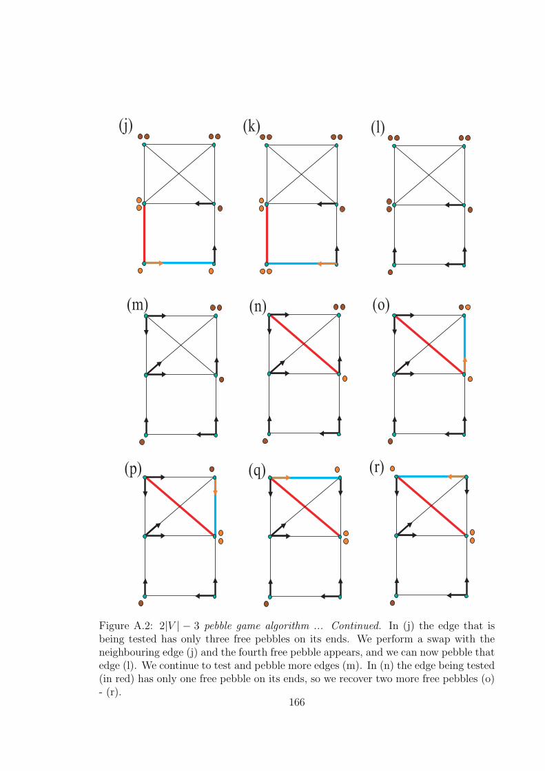
(j) (k) (l)

(m) (n) (o)

(p) (q) (r)

Figure A.2: 2|V | − 3 pebble game algorithm ... Continued. In (j) the edge that isbeing tested has only three free pebbles on its ends. We perform a swap with theneighbouring edge (j) and the fourth free pebble appears, and we can now pebble thatedge (l). We continue to test and pebble more edges (m). In (n) the edge being tested(in red) has only one free pebble on its ends, so we recover two more free pebbles (o)- (r).

166

(s) (t) (u)

Figure A.3: 2|V | − 3 pebble game algorithm ... Continued. As we cannot recover thefourth free pebble, the last edge is declared redundant (indicated as a dashed line)(u). The graph is flexible as it has four remaining free pebbles.

167

References

[1] B. Alberts, A. Johnson, J. Lewis, M. Raff, K. Roberts and P. Walter, Molecular

Biology of the Cell, Garland Science, New York, Fourth Edition, 2002.

[2] B. D. O. Anderson, P. N. Belhumer, T. Eren, A. S. Morse and W. Whiteley, Op-

erations on rigid formations of autonomous agents, Comunicatios in Informations

and Systems, Vol. 3, No. 4, p. 223–258, 2004.

[3] M.E. Barnes and W. Whiteley, Preprint, York University, 2005.

[4] C. Brandon and J. Tooze, Introduction to Protein Structure. Garland Publishing,

New York, London, 1999.

[5] The Brookhaven Protein Data Bank (PDB), http://www.pdb.bnl.gov

[6] J.P. Changeux, F. Jacob and J. Monod, Allosteric proteins and cellular control

systems, J Mol Biol, 6:306-329, 1963.

[7] M. Chubynsky, B.M. Hespenheide, D.J. Jacobs, L.A. Kuhn, M.L., S.Menor, A.J.

Rader, M.F. Thorpe, W Whiteley and M.I. Zavodszky, Constraint Theory ap-

plied to Proteins. To be published in the proceedings of the Indo-US Biopolymer

workshop by Nova Publisher, 2004.

[8] T.H. Cormen, C.E. Leiserson, R.L. Rivest and C. Stein, Introduction to Algo-

rithms, The MIT Press, Cambridge, Massachusetts, Second Edition, 2001.

168

[9] B. S. DeDecker, Allosteric Drugs: thinking outside the active-site box, Chem

Biol, 7:R103-R107, 2000.

[10] R. Diestel, Graph Theory, Springer-Verlag, New York, Second Edition, 2000.

[11] Flexweb Server (FIRST), http://flexweb.asu.edu

[12] Database of Macromolecular Movements, http://www.molmovdb.org

[13] M. Gerstein, A.M. Lesk, C. Chothia, Structural mechanisms for domain move-

ments, Biochemistry, 33:6739-6749, 1994.

[14] H. Gluck, Almost all simply connected closed surfaces are rigid, In Geometric

Topology, Lecture notes in Mathematics, Springer-Verlag, Berlin, No. 438, p.

225–239, 1975.

[15] J. Graver, B. Servatius, and H. Servatius, Combinatorial Rigidity, Graduate

Studies in Math., AMS, 1993.

[16] J. Graver, Counting on Frameworks: Mathematics to Aid the Design of Rigid

Structures, The Mathematical Association of America, Washington, 2001.

[17] K. Gunasekaran, B. Ma and R. Nussinov, Is Allostery an Intrinsic Property of

all Dynamic Proteins?, 57:433-343, 2004.

[18] S. Hayward, Structural Principles Governing Domain Motions in Proteins, Pro-

teins, 36:425-435, 1999.

[19] J. Heringa, Protein domains, In Encyclopedia of Genetics, Genomics, Proteomics

and Bioinformatics, Vol. 7, Section 6: Comparative Methods for Structure Anal-

ysis and Prediction; Chapter 68, pp. 3283-3297, Wiley Interscience, 2005.

[20] B. Hendrickson, Conditions for unique graph realizations, SIAM J. Comput., 21,

pp. 65-84, 1992.169

[21] B. Hendrickson and D.J. Jacobs, An algorithm for two dimensional rigidity per-

colation: The pebble game, J. Comput. Phys., 137:346-365, 1997.

[22] B.M. Hespenheide, D.J. Jacobs and M.F. Thorpe, Structural rigidity in the cap-

sid assembly of cowpea chlorotic mottle virus, J. Phys.: Condens. Matter 16

S5055-64, 2004.

[23] B. Jackson and T. Jordan, Rank and independence in the rigidity matroid of

molecular graphs, submited (see EGRES Technical Report No. 2006-02).

[24] D.J. Jacobs and M.F. Thorpe, Generic rigidity percolation: The pebble game,

Physical Review Letters, 75:4051-4054, 1995.

[25] D.J. Jacobs and M.F. Thorpe, Generic rigidity percolation in two dimensions,

Physical Review. E. Statistical Physics, Plasmas, Fluids, and Related Interdis-

ciplinary Topics, 53:3682-3693, 1996.

[26] D.J. Jacobs, Generic rigidity in three-dimensional bond-bending networks, Jour-

nal of Physics a-Mathematical and General, 31:6653-6668, 1998.

[27] D.J. Jacobs, L.A. Kuhn and M.F. Thorpe, Flexible and rigid regions in proteins,

in Rigidity theory and applications, M.F. Thorpe and P.M. Duxbury, Editors,

Academic/Kluwer. p. 357-384, 1999.

[28] D.J. Jacobs, L.A. Kuhn, A.J. Rader and M.F. Thorpe, Protein flexibility and

dynamics using constraint theory, J Mol Graph Model, 19:60-9,2003.

[29] D.J. Jacobs, private communication.

[30] L.E. Kavraki, G.N. Phillips JR. and M.L. Teodoro, Journal of Computational

Biology, Volume 10, Numbers 34, p. 617-634, 2003.

170

[31] L.A. Kuhn, A. Mantler, B. Servatius, J. Snoeyink, I. Streinu and W. Whiteley,

Preprint, 2004.

[32] L.A. Kuhn, D.J. Rader and M.F. Thorpe, Protein flexibility predictions using

graph theory, Proteins, 44:150-65, 2001.

[33] L.A. Kuhn, ProFlex, http://www.bch.msu.edu/labs/kuhn/web/software.html,

2004.

[34] G. Laman, On graphs and rigidity of plane skeletal structures, J. Eng. Mathe-

matics, 4:331-340, 1970.

[35] S. Law, Predicting CDR flexibility in immunoglobulin, Honour’s thesis, 2005.

[36] A. Lee and I. Streinu, Pebble Game Algorithms for Graph Arboricity, Preprint,

Smith College, 2005.

[37] T. Mamonova, B.M. Hespenheide , R. Straub, M.F. Thorpe and M. Kurnikova,

Phys. Bio. 2, S137-47, 2005.

[38] A. Mantler and J. Snoeynik, Banana Spiders: A study of connectivity in 3D

combinatorial rigidity, CCCG, 44-47, 2004.

[39] J.C. Maxwell, On reciprocal figures and diagrams of forces, Phil. Mag., 27:250-

261, 1864.

[40] C. Moukarzel, An efficient algorithm for testing the generic rigidity of graphs in

the plane, J. Phys. A: Math. Gen., 29 8079-98, 1996.

[41] R. Nussinov, N. Sinha and C.J. Tsai, Building Blocks, Hinge-Bending Motions

and Protein Topology. Volume 19, Issue Number 3, p. 369-380, 2001.

[42] PYMOL, http://pymol.sourceforge.net/

171

[43] RasMol, http://www.umass.edu/microbio/rasmol/

[44] A. Recski, Matroid Theory and its Applications, Springer-Verlag, Berlin, 1989.

[45] K. Schulten and W. Wriggers, Protein Domain Movements: Detection of Rigid

Domains and Visualization of Hinges in Comparison of Atomic Coordinates,

Proteins, 29:1-14, 1997.

[46] W. Scott, C. Schiffer, Curling of flap tips in HIV-1 protease as a mechanism for

substrate entry and tolerance of drug resistance, Struct Fold Design, 9:1259-1265,

2000.

[47] B. Servatius and H. Servatius, Generic and Abstract Rigidity, Rigidity theory

and applications, M.F. Thorpe and P.M. Duxbury, Editors, Academic/Kluwer.

p. 1-19, 1999.

[48] K. Sugihara, On redundant bracing in plane skeletal structures, Bull. Electrotech.

Lab. 44, 376 (1980).

[49] T.S. Tay, Rigidity of Multigraphs I: Linking Rigid Bodies in n-space, Journal of

Combinatorial Theory Series B, Vol. 26, pp. 95-112, 1984.

[50] T.S. Tay and W. Whiteley, Generating Isostatic Frameworks, Structural Topol-

ogy 11, 21-69, 1985.

[51] M. F. Thorpe, Rigidity percolation Physics of Disordered Materials (Institute

for Amorphous Studies Series) (New York: Plenum), 1985.

[52] M.F. Thorpe, Protein Folding, HIV and Drug Design Physics and Technology

Forefronts, APS News, February, 2003.

[53] W.T. Tutte, On the problem of decomposing a graph into n connected factors.

Journal London Math. Soc., 142:221-230, 1961.172

[54] S. Wells, private communication.

[55] N. White, Encyclopedia of Mathematics and its Applications: Theory of Ma-

troids, Cambridge University Press, Cambridge, 1986.

[56] W. Whiteley, Some Matroids from discrete applied geometry. In J. Bonin, J.

Oxley, and B. Servatius, editors, Matroid Theory, volume 197 of Contemp. Math.,

pages 171-311. Amer. Math. Soc., Providence, 1996.

[57] W. Whiteley, Rigidity of molecular structures: generic and geometric analysis,

Rigidity theory and applications, M.F. Thorpe and P.M. Duxbury, Editors, Aca-

demic/Kluwer. p. 21-46, 1999.

[58] W. Whiteley, Rigidity and scene analysis, In J. Goodman and J. ORourke, ed-

itors, Handbook of Discrete and Computational Geometry, chapter 60, pages

1327–1354. Chapman Hall/CRC Press, Boca Raton, FL, 2nd edition, 2004.

[59] W. Whiteley, private communication.

[60] W. Whiteley, Counting out to the flexibility of molecules, Phys. Biol. 2, S116-

S126, 2005.

173