Counting Trees in Supersymmetric Quantum

Mechanics

Clay Cordova1∗ and Shu-Heng Shao2†

1Society of Fellows, Harvard University, Cambridge, MA, USA

2Jefferson Physical Laboratory, Harvard University, Cambridge, MA, USA

Abstract

We study the supersymmetric ground states of the Kronecker model of quiver quantummechanics. This is the simplest quiver with two gauge groups and bifundamental matterfields, and appears universally in four-dimensional N = 2 systems. The ground statedegeneracy may be written as a multi-dimensional contour integral, and the enumerationof poles can be simply phrased as counting bipartite trees. We solve this combinatoricsproblem, thereby obtaining exact formulas for the degeneracies of an infinite class of models.We also develop an algorithm to compute the angular momentum of the ground states, andpresent explicit expressions for the refined indices of theories where one rank is small.

February 2015

∗e-mail: cordova@physics.harvard.edu†e-mail: shshao@physics.harvard.edu

arX

iv:1

502.

0805

0v2

[he

p-th

] 2

Mar

201

5

Contents

1 Introduction 2

2 Kronecker Quivers 4

2.1 Kronecker Moduli and the Index . . . . . . . . . . . . . . . . . . . . . . . . . 5

2.1.1 The Grassmannian as a Kronecker Moduli Space . . . . . . . . . . . 7

2.1.2 Moduli Spaces as a Function of k . . . . . . . . . . . . . . . . . . . . 8

2.2 The Degeneration Formula and Star Quivers . . . . . . . . . . . . . . . . . . 8

2.3 The Graph Theory Problem: Counting Trees . . . . . . . . . . . . . . . . . . 10

2.3.1 The Tree Counting Theorem and T (~Lm∗,r) . . . . . . . . . . . . . . . 12

2.4 An Index Formula for the Kronecker Quiver (M,Mr + 1) . . . . . . . . . . . 14

3 Analysis of the Index Formula 15

3.1 Simplifications at Special Values of r . . . . . . . . . . . . . . . . . . . . . . 15

3.1.1 Recovering the Grassmannian Index . . . . . . . . . . . . . . . . . . . 15

3.1.2 The Case r = 1 . . . . . . . . . . . . . . . . . . . . . . . . . . . . . . 15

3.2 Symmetries of the Index Formula . . . . . . . . . . . . . . . . . . . . . . . . 17

3.3 Comparison to Wall-Crossing Formulas . . . . . . . . . . . . . . . . . . . . . 18

4 Bipartite Graphs from Contour Integrals 20

4.1 A Residue for the Star Quiver . . . . . . . . . . . . . . . . . . . . . . . . . . 20

4.2 The Jeffrey-Kirwan Rule . . . . . . . . . . . . . . . . . . . . . . . . . . . . . 23

4.3 From Poles to Bipartite Graphs . . . . . . . . . . . . . . . . . . . . . . . . . 25

4.4 From Bipartite Graphs to Poles: The Tree Rule . . . . . . . . . . . . . . . . 28

5 Graph Theory 31

5.1 Generalities in Graph Theory . . . . . . . . . . . . . . . . . . . . . . . . . . 31

5.2 Division of Bipartite Graphs . . . . . . . . . . . . . . . . . . . . . . . . . . . 32

5.3 Proof of the Tree Counting Theorem . . . . . . . . . . . . . . . . . . . . . . 35

6 Computations of the Refined Index 43

6.1 Example: (2, 1) . . . . . . . . . . . . . . . . . . . . . . . . . . . . . . . . . . 44

6.2 Example: (2, 2r + 1) . . . . . . . . . . . . . . . . . . . . . . . . . . . . . . . 47

A An Identity for [xM ]exp(βF ) When r = 1 51

B Degenerate Poles 53

1

1 Introduction

One of the most basic problems in any quantum system is to determine the spectrum of

stable states. However, outside the realm of perturbation theory and exactly solvable mod-

els the answer to this question is elusive. One class of examples where progress is possible

are those enjoying supersymmetry. In general, these models are not exactly solvable, yet

nevertheless there are states in the spectrum whose existence and properties can be reliably

determined. These supersymmetric models yield a window into non-perturbative physics

where strong coupling phenomena may be confronted analytically. In particular, field the-

ories and gravities with extended supersymmetry provide a class of models where exact

spectroscopy results are feasible.

Motivated by these general considerations, in this work we analyze in detail a non-trivial

model of supersymmetric particle spectroscopy. We consider a non-relativistic quantum

mechanical system with two distinct species of (super)particles, and four supercharges.

Each particle carries minimal angular momentum, and electromagnetic charges γ1 and γ2.

The low-energy interactions of the system are invariantly characterized by the integral Dirac

pairing of the electromagnetic charges

〈γ1, γ2〉 = k > 0 . (1.1)

Our aim is to determine the non-relativistic bound state spectrum formed by M particles

of type one, and N particles of type two. The system and its interactions are encoded

in a quiver diagram, known as the Kronecker quiver shown below.1 We study only those

M Nk

//

Figure 1: The Kronecker quiver with dimension vector (M,N) and k arrows. The quiverencodes the interaction of M particles of charge γ1 and N particles of charge γ2 with〈γ1, γ2〉 = k.

bound states which preserve all four supercharges. These are the supersymmetric ground

states of this quiver quantum mechanics. We denote their degeneracy by Ω(M,N, k). The

Kronecker quiver model and the degeneracies Ω(M,N, k), have been previously studied

from a variety of perspectives, including quantum groups [2], wall-crossing formulas [3–5],

spectral networks [6], and equivariant cohomology [7, 8].

Our main result, described in detail in §2 and §3, is a formula for Ω(M,N, k) in the

special case where the parameter N may be expressed as N = Mr + 1 for non-negative

integer r. It is simplest to state our results in terms of a generating function. Introduce

1The explicit expression for the Hamiltonian of this system may be found, for instance, in [1].

2

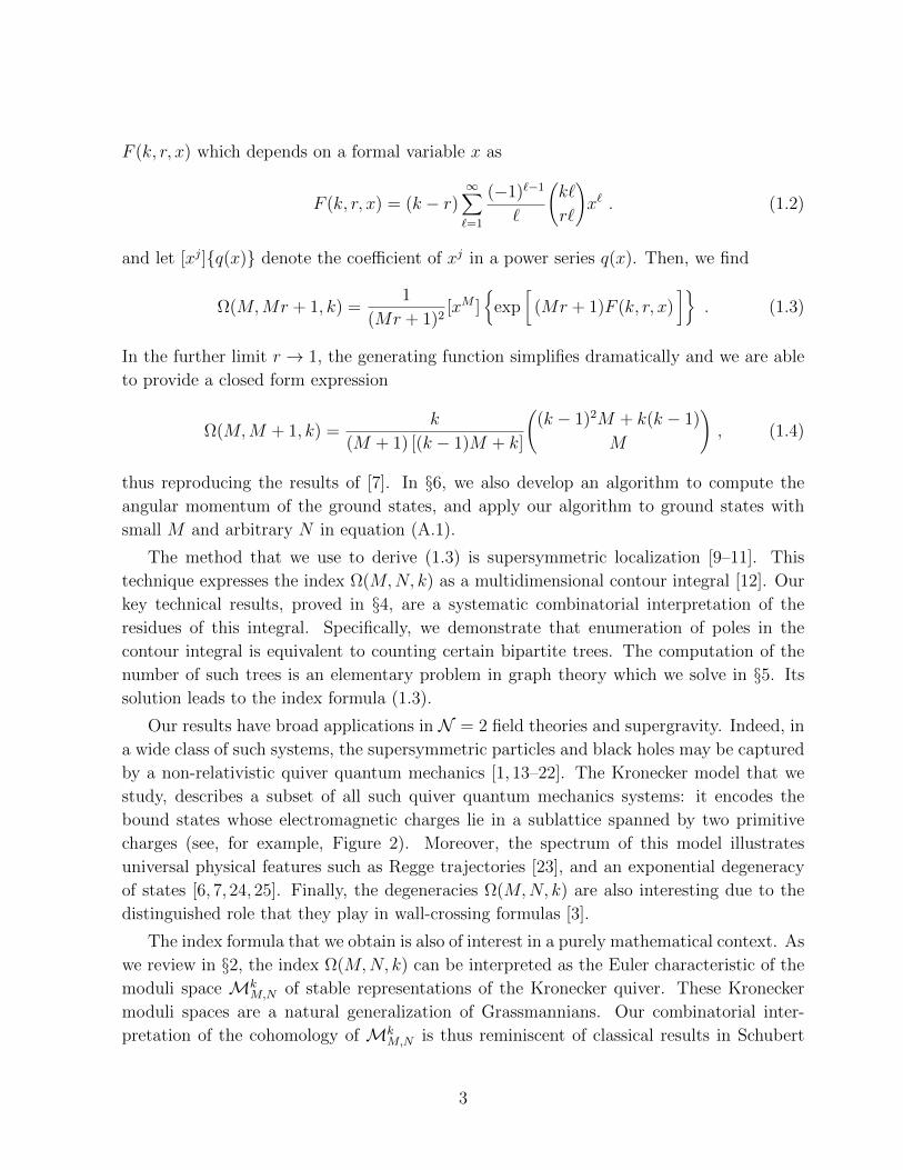
F (k, r, x) which depends on a formal variable x as

F (k, r, x) = (k − r)∞∑`=1

(−1)`−1

`

(k`

r`

)x` . (1.2)

and let [xj]q(x) denote the coefficient of xj in a power series q(x). Then, we find

Ω(M,Mr + 1, k) =1

(Mr + 1)2[xM ]

exp

[(Mr + 1)F (k, r, x)

]. (1.3)

In the further limit r → 1, the generating function simplifies dramatically and we are able

to provide a closed form expression

Ω(M,M + 1, k) =k

(M + 1) [(k − 1)M + k]

((k − 1)2M + k(k − 1)

M

), (1.4)

thus reproducing the results of [7]. In §6, we also develop an algorithm to compute the

angular momentum of the ground states, and apply our algorithm to ground states with

small M and arbitrary N in equation (A.1).

The method that we use to derive (1.3) is supersymmetric localization [9–11]. This

technique expresses the index Ω(M,N, k) as a multidimensional contour integral [12]. Our

key technical results, proved in §4, are a systematic combinatorial interpretation of the

residues of this integral. Specifically, we demonstrate that enumeration of poles in the

contour integral is equivalent to counting certain bipartite trees. The computation of the

number of such trees is an elementary problem in graph theory which we solve in §5. Its

solution leads to the index formula (1.3).

Our results have broad applications in N = 2 field theories and supergravity. Indeed, in

a wide class of such systems, the supersymmetric particles and black holes may be captured

by a non-relativistic quiver quantum mechanics [1, 13–22]. The Kronecker model that we

study, describes a subset of all such quiver quantum mechanics systems: it encodes the

bound states whose electromagnetic charges lie in a sublattice spanned by two primitive

charges (see, for example, Figure 2). Moreover, the spectrum of this model illustrates

universal physical features such as Regge trajectories [23], and an exponential degeneracy

of states [6, 7, 24, 25]. Finally, the degeneracies Ω(M,N, k) are also interesting due to the

distinguished role that they play in wall-crossing formulas [3].

The index formula that we obtain is also of interest in a purely mathematical context. As

we review in §2, the index Ω(M,N, k) can be interpreted as the Euler characteristic of the

moduli space MkM,N of stable representations of the Kronecker quiver. These Kronecker

moduli spaces are a natural generalization of Grassmannians. Our combinatorial inter-

pretation of the cohomology of MkM,N is thus reminiscent of classical results in Schubert

3

M N//

(a)

M N////

(b)

N1 N2

N3

*4|

Tb

(c)

Figure 2: Examples of Kronecker quivers occur in many well-known models. The casek = 1, illustrated in (a), describes the spectrum of the Argyres-Douglas conformal fieldtheory [26–28]. The case k = 2, illustrated in (b), describes the spectrum of su(2) Seiberg-Witten theory [16, 29]. The case k > 2 occurs frequently as a subset of the bound statesin many N = 2 systems. For instance, the k = 3 case in (c) appears in the quiver thatdescribes the bound states of D-branes in type IIA string theory on local P2 [14]. Moregenerally, all Kronecker quivers with k > 2 occur as subsectors of the quiver describingbound states in su(N) super-Yang-Mills [6].

calculus.

There are a number of significant questions left unanswered by our analysis. Most glar-

ingly, it would be interesting to extend our result (1.3) to the general value of parameters

(M,N, k), and thereby provide a complete solution to the Kronecker model. More concep-

tually, the exponential resummation appearing in (1.3) is qualitatively similar to the general

relationship between Donaldson-Thomas invariants and Gromov-Witten invariants [30,31].

This suggests, perhaps, that the function F (k, r, x) itself admits a direct enumerative mean-

ing. Finally, it would be satisfying to explain the physical significance of the bipartite trees

which play a crucial technical role in this work, perhaps by relating them to attractor flow

trees [32, 33]. We leave these problems as potential avenues for future investigation.

2 Kronecker Quivers

In this section, we give an overview of our main result for the degeneracies Ω(M,N, k).

Complete proofs of all ingredients presented may be found in §4 and §5.

We begin in §2.1 with a review of the geometry underlying the indices of the Kronecker

quiver, and explain how the degeneracies Ω(M,N, k) may be viewed as the Euler charac-

teristic of the Kroncker moduli space. Next in §2.2 and §2.3 we overview the main steps

in our calculation. In particular, we describe how counting bipartite trees is related to

computing indices and in §2.3.1 we state a theorem which enables us to enumerate all such

trees. Finally, in §2.4 we assemble the pieces into a formula for Ω(M,N, k), in the special

case N = Mr + 1.

4

2.1 Kronecker Moduli and the Index

In any model of quiver quantum mechanics with four supercharges, the problem of deter-

mining the ground state spectrum can be phrased in a completely geometric language in

terms of quiver moduli spaces. In this section we review this connection in the context of

the Kronecker quiver.

Consider the Kronecker quiver illustrated in Figure 1. The Lagrangian for this system

is a gauged N = 4 quantum mechanics. Each node supports a unitary gauge group of ranks

M and N respectively with associated vector multiplets, while the arrows of the quiver are

bifundametal chiral multiplet matter fields. The explicit expression for the Hamiltonian of

this system may be found, for instance, in [1].

The system has a classical Higgs branch moduli space MkM,N described in a standard

way. The chiral multiplet fields Φi (i = 1, · · · , k) have constant expectation values. Thus,

they may be viewed as specifying linear maps

Φi : CM → CN . (2.1)

On the set of possible field expectation values we impose the D-term equations

k∑i=1

Φ†i Φi = ζIM ,k∑i=1

Φi Φ†i =Mζ

NIN , (2.2)

where in the above, ζ > 0 is the Fayet-Iliopoulos parameter,2 and IL is the L× L identity

matrix. Finally, the locus of solutions to the D-term equation (2.2) is invariant under the

action of the gauge group U(M)× U(N) acting on the Φi via the bifundamental represen-

tation. The desired moduli space MkM,N is the quotient space

MkM,N ≡

Φi

∣∣∣∣∣∣k∑i=1

Φ†i Φi = ζIM ,k∑i=1

Φi Φ†i =Mζ

NIN

/U(M)× U(N) . (2.3)

The Kronecker moduli spaces MkM,N have several features which follow directly from

their construction as quotients, as well as through the application of Seiberg dualities (quiver

mutations [34,35]). We state these facts here. Throughout this discussion, we assume that

the pair (M,N) are coprime, to avoid various subtleties.

• The moduli space MkM,N is a smooth compact Kaher manifold (if it is non-empty),

with metric inherited via its construction as a Kaher quotient.

2When ζ < 0 all moduli spaces are empty, illustrating the wall-crossing phenomenon.

5

• The complex dimension of MkM,N is

dim(MkM,N) = kNM −M2 −N2 + 1 . (2.4)

In particular, the moduli space is non-empty if and only if the above dimension

formula is non-negative.

• In the Hodge decomposition of the cohomology of MkM,N , we have [2]

p 6= q =⇒ hp,q(Mk

M,N

)= 0 . (2.5)

• We have the following isomorphisms

Reflection: MkM,N∼=Mk

N,M ,

Mutation: MkM,N∼=Mk

N,Nk−M .(2.6)

According to familiar results in supersymmetric quantum mechanics, the supersymmet-

ric ground states may be extracted from the cohomology of the moduli space. Moreover, the

data of the spin of ground states (an su(2) representation) is determined by the Lefschetz

su(2) action on the cohomology.

Complete information about the ground state spectrum is conveniently packaged into a

refined index depending on a fugacity y which encodes the angular momentum

Ω(M,N, k, y) ≡d∑p=0

y2p−d hp,p(MkM,N) , (2.7)

where in the above, d denotes the complex dimension of the moduli space given in (2.4). Up

to the overall factor of y−d, this index coincides with the Hirzebruch χy genus. In particular,

in the specialization y → 1 the above reduces to the Euler characteristic

Ω(M,N, k) ≡ Ω(M,N, k, 1) =d∑p=0

hp,p(MkM,N) = χ

(Mk

M,N

). (2.8)

One notable feature of both (2.7) and (2.8) is that the Betti numbers are weighted without

signs. Thus, Ω(M,N, k, y), which a priori is an index and counts states up to signs, in fact

computes the exact degeneracy due to the vanishing result (2.5) on the cohomology.3

The indices (2.8) and (2.7) are the quantities that we compute in this work. Our main

results concern the Euler characteristic (2.8). In §6 we present an algorithm to determine

the complete cohomology generating function (2.7).

3This is a special case of the “No-Exotics” conjecture [36,37].

6

2.1.1 The Grassmannian as a Kronecker Moduli Space

In this section we provide some intuition for Kronecker moduli spaces, by demonstrating

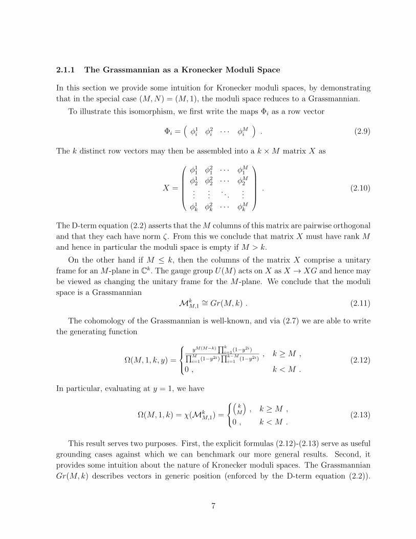
that in the special case (M,N) = (M, 1), the moduli space reduces to a Grassmannian.

To illustrate this isomorphism, we first write the maps Φi as a row vector

Φi =(φ1i φ2

i · · · φMi). (2.9)

The k distinct row vectors may then be assembled into a k ×M matrix X as

X =

φ1

1 φ21 · · · φM1

φ12 φ2

2 · · · φM2...

.... . .

...

φ1k φ2

k · · · φMk

. (2.10)

The D-term equation (2.2) asserts that theM columns of this matrix are pairwise orthogonal

and that they each have norm ζ. From this we conclude that matrix X must have rank M

and hence in particular the moduli space is empty if M > k.

On the other hand if M ≤ k, then the columns of the matrix X comprise a unitary

frame for an M -plane in Ck. The gauge group U(M) acts on X as X → XG and hence may

be viewed as changing the unitary frame for the M -plane. We conclude that the moduli

space is a Grassmannian

MkM,1∼= Gr(M,k) . (2.11)

The cohomology of the Grassmannian is well-known, and via (2.7) we are able to write

the generating function

Ω(M, 1, k, y) =

yM(M−k)

∏k

i=1(1−y2i)∏M

i=1(1−y2i)

∏k−M

i=1(1−y2i)

, k ≥M ,

0 , k < M .(2.12)

In particular, evaluating at y = 1, we have

Ω(M, 1, k) = χ(MkM,1) =

(kM

), k ≥M ,

0 , k < M .(2.13)

This result serves two purposes. First, the explicit formulas (2.12)-(2.13) serve as useful

grounding cases against which we can benchmark our more general results. Second, it

provides some intuition about the nature of Kronecker moduli spaces. The Grassmannian

Gr(M,k) describes vectors in generic position (enforced by the D-term equation (2.2)).

7

The Kronecker moduli spaces MkM,N generalize this idea, and describe configurations of

matrices in general position.

2.1.2 Moduli Spaces as a Function of k

Another way to gain intuition about Kronecker moduli spaces is to examine them as a

function of the number of arrows k. Consider the special case M = N . Then, the moduli

space describes k linear maps

Φi : CM → CM . (2.14)

As a consequence of the D-term equation, these maps are in general position and hence, on

an open set in the moduli space, at least one of them is invertible. One may then fix some

of the gauge redundancy by going to a basis where this invertible map is the identity.

What remains after this is k−1 linear maps, where now the remaining gauge redundancy

acts as conjugation. For k = 1 this problem is trivial. For k = 2, this problem is solved

by the Jordan decomposition theorem. Correspondingly, for k = 1, 2 all Kronecker moduli

spaces may be explicitly determined.

Finally, for k > 2 these moduli spaces parameterize multiple linear maps up to conju-

gation. This is a notoriously wild representation theory problem, and there is no known

general description of the moduli spaceMkM,N . Despite the complexity for large k, we will

be able to obtain simple exact formulas for the numerical invariants of these moduli spaces.

2.2 The Degeneration Formula and Star Quivers

In order to determine a formula for the Euler characteristic of Kronecker moduli space, it

is useful to reduce it to a sum of Euler characteristics of simpler spaces. This is achieved

with the MPS degeneration formula [38] (see also [39]).

Physically speaking, the MPS degeneration formula expresses the bound states as a

sum of contributions where the M particles of type one group into clumps, each of which

subsequently interact and form bound states with the remaining particles of type two.

Weighting each contribution appropriately, we determine that the Euler characteristic of

the Kronecker moduli space may be written as

Ω(M,N, k) = χ(MkM,N) =

∑m∗`M

[M∏`=1

1

m`!

((−1)`−1

`2

)m`]χ(Mk

m∗,N) , (2.15)

8

where the sum is over all partitions m∗ = (m1, · · · ,mM) of M ,

M∑`=1

`m` = M, m` ∈ N ∪ 0 . (2.16)

The main actor in the degeneration formula, is the Euler characteristic of the space

Mkm∗,N . This is the quiver moduli space of the “star quiver” (Figure 3) associated to the

partition m∗. It has a central non-abelian node with rank N and∑M`=1m` abelian nodes

surrounding the non-abelian node. Among all the abelian nodes, m` of them have `k arrows

pointing to the non-abelian node for each ` = 1, · · · ,M (m` may vanish).

M Nk

// =∑m∗`M

c(m∗) N1

1

1

1

11

`k

. ..

...`k

m`

k

2k

...m2· · · 2k

· · · k

m1︷︸︸︷

//::

oo

dd

Figure 3: A graphical representation of the MPS degeneration formula (2.15). The Eulercharacteristic of the Kronecker moduli space can be expressed as a sum of Euler charac-teristics of star quivers, each associated to a partition of M . The contribution of each star

quiver is weighted with a combinatorial coefficient c(m∗) =∏M`=1

1m`!

((−1)`−1

`2

)m`

.

As a result of the degeneration formula (2.15), the task of computing the Euler char-

acteristic of Kronecker moduli space is reduced to determining the Euler characteristics of

star quivers. We carry out this task using the supersymmetric localization formula which

expresses the Euler characteristic of quiver moduli spaces as a Jeffrey-Kirwan residue inte-

gral [10, 11].

In the case of the star quiver associated to the partition m∗ ` M with general (M,N),

the combinatorics of the residues is involved. However in the special case

N = Mr + 1 , (2.17)

9

for some non-negative integer r, the combinatorics simplifies to an elementary problem in

graph theory. From now on, we restrict our analysis to the special case where (2.17) holds.

In the remainder of this section we describe the resulting correspondence between residues

and graphs, and state the solution to the resulting counting problem. Complete proofs are

deferred to §4 and §5 respectively.

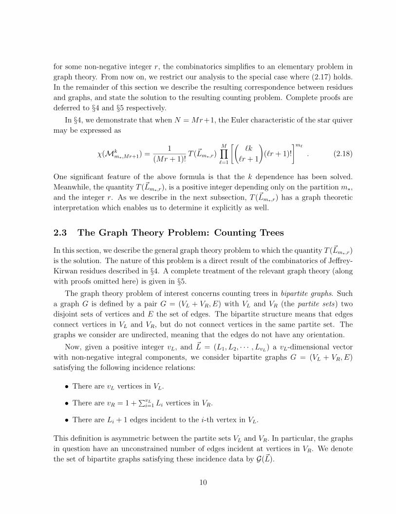
In §4, we demonstrate that when N = Mr+1, the Euler characteristic of the star quiver

may be expressed as

χ(Mkm∗,Mr+1) =

1

(Mr + 1)!T (~Lm∗,r)

M∏`=1

[(`k

`r + 1

)(`r + 1)!

]m`

. (2.18)

One significant feature of the above formula is that the k dependence has been solved.

Meanwhile, the quantity T (~Lm∗,r), is a positive integer depending only on the partition m∗,

and the integer r. As we describe in the next subsection, T (~Lm∗,r) has a graph theoretic

interpretation which enables us to determine it explicitly as well.

2.3 The Graph Theory Problem: Counting Trees

In this section, we describe the general graph theory problem to which the quantity T (~Lm∗,r)

is the solution. The nature of this problem is a direct result of the combinatorics of Jeffrey-

Kirwan residues described in §4. A complete treatment of the relevant graph theory (along

with proofs omitted here) is given in §5.

The graph theory problem of interest concerns counting trees in bipartite graphs. Such

a graph G is defined by a pair G = (VL + VR, E) with VL and VR (the partite sets) two

disjoint sets of vertices and E the set of edges. The bipartite structure means that edges

connect vertices in VL and VR, but do not connect vertices in the same partite set. The

graphs we consider are undirected, meaning that the edges do not have any orientation.

Now, given a positive integer vL, and ~L = (L1, L2, · · · , LvL) a vL-dimensional vector

with non-negative integral components, we consider bipartite graphs G = (VL + VR, E)

satisfying the following incidence relations:

• There are vL vertices in VL.

• There are vR = 1 +∑vLi=1 Li vertices in VR.

• There are Li + 1 edges incident to the i-th vertex in VL.

This definition is asymmetric between the partite sets VL and VR. In particular, the graphs

in question have an unconstrained number of edges incident at vertices in VR. We denote

the set of bipartite graphs satisfying these incidence data by G(~L).

10

VL VR

1 •

L1 + 1

· · · • 1

2 • L2 + 1 • 2

· · ·

......

vL •

LvL + 1

· · · • vR

Figure 4: A bipartite graph G in the set G(~L) defined by a vL-dimensional vector ~L =(L1, · · · , LvL) with Li ∈ N ∪ 0. (The connections between partite sets are not shown.)There are vL vertices in VL and vR = 1 +

∑i Li vertices in VR. The i-th vertex in VL is

incident to Li + 1 edges. The number of edges for a vertex in VR is not constrained. Thetotal number of edges is e = vL +

∑i Li = vL + vR− 1. The quantity of interest T (~L) is the

number of trees (connected graphs with no cycle) in the set of bipartite graphs G(~L).

Define a tree, to be a connected graph with no cycles. The main quantity of interest is

then

T (~L) = number of trees in G(~L) . (2.19)

The incidence data defining the bipartite graphs G(~L) are tuned in such a way as to make

the number of trees non-zero. Indeed, using vR = 1 +∑i Li, the total number of edges e is

related to the total number of vertices v = vL + vR by

e =vL∑i=1

(1 + Li) = vL + vR − 1 = v − 1 . (2.20)

By an elementary proposition in graph theory (see Proposition 1 in §5), a tree has precisely

v−1 edges. Hence it is precisely for this choice of vR that the set of trees can be non-empty.

We illustrate these definitions in several examples below.

11

Example: vL = 1, ~L = (L1)

The simplest example has a single left vertex (vL = 1) and ~L = (L1) a one-dimensional

vector for some non-negative integer L1. In this case vR = L1 + 1 and the number of edges

e = L1 + 1. For G ∈ G(~L), there are L1 + 1 edges incident to the vertex in VL. There is a

unique tree in G(~L) shown in Figure 5.

VL VR

1 • • 1

• 2

...

• L1 + 1

Figure 5: An example of a tree in G(~L) with ~L = (L1). We have vL = 1 vertex in VL andvR = L1 + 1 in VR, with a total number of e = L1 + 1 edges. The vertex in VL is incidentto L1 + 1 edges. This is the unique tree in G(~L), i.e. T (~L) = 1.

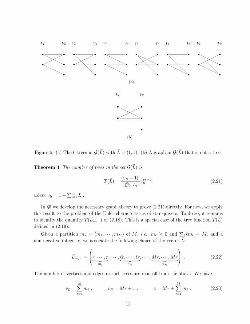
Example: vL = 2, ~L = (1, 1)

As a more advanced example, consider the case with two left vertices (vL = 2) and~L = (1, 1) in Figure 6a. There are three right vertices (vR = 3) and four total edges (

e = 4). Each of the vertices in VL is incident to 2 edges. There are 6 trees in G(~L) shown

in Figure 6a, i.e. T (~L) = 6.

2.3.1 The Tree Counting Theorem and T (~Lm∗,r)

One of the remarkable facts about trees is that given any incidence data defining the set of

bipartite graphs G(~L), the number of trees T (~L) can be exactly determined. The result is

a key theorem:4

4We thank Fan Wei and Yu-Wei Fan for pointing out that this theorem appears in the textbook [40].

12

VL VR

• •

• •

•

VL VR

• •

• •

•

VL VR

• •

• •

•

VL VR

• •

• •

•

VL VR

• •

• •

•

VL VR

• •

• •

•

(a)

VL VR

• •

• •

•

(b)

Figure 6: (a) The 6 trees in G(~L) with ~L = (1, 1). (b) A graph in G(~L) that is not a tree.

Theorem 1 The number of trees in the set G(~L) is

T (~L) =(vR − 1)!∏vL

i=1 Li!vvL−1R , (2.21)

where vR = 1 +∑vLi=1 Li.

In §5 we develop the necessary graph theory to prove (2.21) directly. For now, we apply

this result to the problem of the Euler characteristics of star quivers. To do so, it remains

to identify the quantity T (~Lm∗,r) of (2.18). This is a special case of the tree function T (~L)

defined in (2.19).

Given a partition m∗ = (m1, · · · ,mM) of M , i.e. m` ≥ 0 and∑` `m` = M , and a

non-negative integer r, we associate the following choice of the vector ~L:

~Lm∗,r =

r, · · · , r︸ ︷︷ ︸m1

, · · · , `r, · · · , `r︸ ︷︷ ︸m`

, · · · ,Mr, · · · ,Mr︸ ︷︷ ︸mM

. (2.22)

The number of vertices and edges in such trees are read off from the above. We have

vL =M∑`=1

m` , vR = Mr + 1 , e = Mr +M∑`=1

m` . (2.23)

13

These quantities are related to the physical parameters defining the star quiver of Figure

3. In particular, vL is the number of abelian nodes, while vR is the rank of the central non-

abelian node. Finally, the structure of ~Lm∗,r emerges from the pattern of Fayet-Iliopoulos

parameters as derived in §4.

Applying the tree counting theorem 1 we conclude that the number of bipartite trees

with this incidence data is given by

T (~Lm∗,r) =(Mr)!∏M`=1(`r)!m`

(Mr + 1)∑

`m`−1 . (2.24)

2.4 An Index Formula for the Kronecker Quiver (M,Mr + 1)

Armed with an explicit expression for T (~Lm∗,r) and the factorization formula (2.18), we

are now ready to present our main result. The index for the Kronecker quiver quantum

mechanics with dimension vector (M,Mr + 1) and k arrows is:

χ(MkM,Mr+1) =

1

(Mr + 1)2

∑m∗`M

M∏`=1

1

m`!

[(−1)`−1

`2

(`k

`r + 1

)(Mr + 1)(`r + 1)

]m`

, (2.25)

where the sum is over the partitions m∗ = (m1, m2, · · · , mM) of M , i.e.∑` `m` = M and

m` ∈ N ∪ 0.The expression (2.25) may be simplified with the help of an exponential resummation

and the introduction of a generating function. Introduce the function

F (k, r, x) = (k − r)∞∑`=1

(−1)`−1

`

(k`

r`

)x` , (2.26)

and let [xj]q(x) denote the coefficient of xj in a power series q(x). Then, using the identity

∞∑M=0

∑m∗`M

M∏`=1

1

m`!

(p(`)x`

)m`= exp

[ ∞∑`=1

p(`)x`], (2.27)

we can express (2.25) as

Ω(M,Mr + 1, k) = χ(MkM,Mr+1) =

1

(Mr + 1)2[xM ]

exp

[(Mr + 1)F (k, r, x)

].

(2.28)

This is our final result for the general Euler characteristic of Kronecker moduli space.

14

3 Analysis of the Index Formula

In this section, we provide a number of checks on the index formula.

In §3.1 we illustrate simplifications that occur in the index formula at special values

of r. Specifically, we recover the Grassmannian index at r = 0 and determine a closed

form expression for the degeneracies when r = 1. In §3.2 we demonstrate that the index

formula satisfies required symmetry properties arising from isomorphisms of Kronecker

moduli spaces. Finally, in §3.3, we directly compare our index result (2.28) to wall-crossing

formulas.

3.1 Simplifications at Special Values of r

In this section we describe simplifications to the Euler characteristic formula which occur

at special values of r.

3.1.1 Recovering the Grassmannian Index

The first check on our result occurs when r = 0. In that case the dimension vector is (M, 1)

and hence as reviewed in §2.1.1, the moduli space is a Grassmannian. Thus, for r = 0

we must recover χ(Gr(M,k)). This is readily verified. Indeed, when r = 0, the function

F (k, r = 0, x) of (2.26) simplifies to

F (k, r = 0, x) = k∞∑`=1

(−1)`−1

`x` = k log(1 + x) . (3.1)

The Euler characteristic of the quiver moduli space MkM,1 is then determined from the

prescription (2.28) as

χ(MkM,1) = [xM ]

exp [F (k, 0, x)]

= [xM ]

(1 + x)k

=

(k

M

), (3.2)

which is indeed the Euler characteristic for the Grassmannian Gr(M,k).

3.1.2 The Case r = 1

The index formula (2.28) also simplifies in the special case r = 1 (as well as the equivalent

case r = k − 1 via (3.11)).

In that case, the function F (k, 1, x) of (2.26) may be rewritten in terms of the generalized

15

binomial series Bk(x) defined as [41]

Bk(x) =∞∑`=0

(k`+ 1

`

)x`

k`+ 1. (3.3)

The generalized binomial series obeys an algebraic identity

Bk(x) = 1 + xBk(x)k , (3.4)

which enables one to easily determine the power series coefficients of Bk(x) raised to an

arbitrary real power

[xm] Bk(x)s =

(mk + s

m

)s

mk + s. (3.5)

In particular, in the s→ 0 limit we then obtain

log (Bk(x)) =∞∑`=1

(k`

`

)x`

k`. (3.6)

From which we deduce that

exp[F (k, 1, x)] = Bk(−x)k(1−k) . (3.7)

Comparison to the index formula (2.28), now yields the following simple expression for

the index

Ω(M,M + 1, k) = χ(MkM,M+1) =

k

(M + 1) [(k − 1)M + k]

((k − 1)2M + k(k − 1)

M

). (3.8)

The result (3.8) was first obtained by Weist [7] by alternative techniques. The fact that we

have reproduced (3.8) using the combinatorics of Jeffrey-Kirwan residues provides a strong

check on our method.

Beyond the direct check provided on our work, the appearance of the generalized bino-

mial series is in and of itself significant. This function, Bk(x), has a natural combinatorial

interpretation as the generating function of rooted k-ary trees. These binomials series also

make an appearance in the generating function of indices Ω(M,M, k) [3, 4, 6]. In that

case, since the dimension vector (M,M) is not coprime, the quiver quantum mechanics

has bound states at threshold. The associated Kronecker quiver moduli spaces have sin-

gularities, and extracting the indices from geometry is delicate. Nevertheless, the resulting

generating function again involves the generalized binomial series and suggests a direct in-

terpretation of the index and bound states in terms of rooted trees, perhaps as attractor

flow trees [32, 33].

16

3.2 Symmetries of the Index Formula

As a further consistency check, in this section we show our formula (2.28) respects the

isomorphisms of the quiver moduli space (2.6):

Ω(M,N, k) = Ω(N,M, k) ,

Ω(M,N, k) = Ω(N,Nk −M,k) .(3.9)

Among all the isomorphisms, the following two infinite families are of particular interest.

Ω(2, 2r + 1, k) = Ω(2, 2(k − r − 1) + 1, k) , (3.10)

and

Ω(M,M + 1, k) = Ω (M + 1, (k − 1)(M + 1) + 1, k) . (3.11)

This is because the dimension vectors on both sides of the isomorphisms are of the special

case N = Mr + 1, for which our formula (2.28) is applicable. We will explicitly prove the

invariance of our formula (2.28) in the following.

The First Isomorphism

For the first isomorphism (3.10), it is easier to use the alternative expression (2.25) for

our formula for the index. Using (2.25), the left-hand-side of (3.10) becomes

Ω(2, 2r + 1, k) = −1

4

(2k

2r + 1

)+

1

2

[k!

r!(k − r − 1)!

]2

. (3.12)

Similarly, the righthand side of (3.10) may be written as

Ω(2, 2(k − r − 1) + 1, k) = −1

4

(2k

2k − 2r − 1

)+

1

2

[(k!

(k − r − 1)!r!

)]2

, (3.13)

which is manifestly the same as (3.12).

The Second Isomorphism

The second isomorphism (3.11) is harder to prove. First let us note the following identity

17

from the definition of F (k, r, x) (2.26),

F (k, k − 1, x) =1

k − 1F (k, 1, x) . (3.14)

Applying our general formula (2.28) to the righthand side of (3.11) , we have

Ω (M + 1, (k − 1)(M + 1) + 1, k)

=1

[(k − 1)(M + 1) + 1]2[xM+1]

exp

[(M + 1 +

1

k − 1

)F (k, 1, x)

],

(3.15)

where we have used the identity (3.14).

The relationship between F and the generalized binomial series in the case r = 1 stated

in equation (3.7) (as well as the direct argument given in Appendix A ) shows that function

F (k, r, x) satisfies the following identity

[xM ]

exp [ βF (k, 1, x) ]

=β

Mk(k − 1)

(k(k − 1)β − (k − 1)M − 1

M − 1

), (3.16)

for any complex number β. Applying (3.16) with β = M + 1 + 1k−1

to (3.15), we have

Ω (M + 1, (k − 1)(M + 1) + 1, k) =1

(k − 1)M + k

k

M + 1

((k − 1)2M + k(k − 1)

M

)= Ω(M,M + 1, k) , (3.17)

where in the last equality we have used the simplified expression (3.8) in the case r = 1.

Hence we have checked that our formula (2.28) respects the isomorphisms (2.6).

3.3 Comparison to Wall-Crossing Formulas

A final check on our results is to directly compare the output to wall-crossing formulas.

This allows us to check our result (2.28) for general r and for M and k sufficiently small.

The wall-crossing formula of [3] allows us to determine the change in the indices Ω(M,N, k)

as the Fayet-Iliopoulos parameters ζ are varied. Mathematically, this is the change in the

Donaldson-Thomas invariants of the quiver, as the stability condition is changed.

In the context of the Kronecker model, the wall-crossing formula is particularly simple

to apply. By changing the sign of the FI parameter ζ of (2.2), we reach a chamber where

all moduli spaces are empty, and no non-trivial bound states can form. The only stable

states are then a single particle of type one, or a single particle of type two. We may use

this simple chamber (ζ < 0) as a seed and apply the wall-crossing formula to determine the

indices in the chamber of interest (ζ > 0).

18

To phrase the wall-crossing computation we first introduce functions KM,N which act

on formal variables[x, y

]as

KM,N

[x, y

]=[x(1− (−1)kMNxMyN)kN , y(1− (−1)kMNxMyN)−kM

]. (3.18)

We also introduce a sign function which detects the parity of the dimension of MkM,N

σ(M,N, k) =

+1 , kMN −M2 −N2 + 1 ≡ 0 (mod 2) ,

−1 , kMN −M2 −N2 + 1 ≡ 1 (mod 2) .(3.19)

The wall-crossing formula asserts that a particular function of [x, y] built via compo-

sitions of the above functions does not depend on the chamber. In the case at hand this

implies that→∏

M,N≥0

Kσ(M,N,k)Ω(M,N,k)M,N = K0,1 K1,0 , (3.20)

Where in the above, the product operation is composition of functions, and the order of

composition is that of decreasing M/N.5

To use the wall-crossing formula, note that the function KM,N differs from the identity

only at order xMyN . Whence if we fix a positive integer Q we may solve (3.20) order by

order by replacing the infinite product with a finite product where only those KM,N are

retained with M+N ≤ Q. Then we may compute the composition as a formal power series

(again only retaining terms differing from the identity up to total order Q). Matching to

the right-hand side, we then solve for all Ω(M,N, k) with M +N ≤ Q.

This procedure is computationally costly to carry out for large Q. However, for Q

sufficiently small, wall-crossing provides a useful crosscheck on our results in the case where

r 6= 0, 1. As an example in Table 1, we present wall-crossing results for r = 2. All indices

computed thus far agree with our general index prescription (2.28), and provides a strong

check on the validity of our result.

5If M1/N1 = M1/N2 then KM1,N1KM2,N2

= KM2,N2KM1,N1

. Also the need to introduce σ is becausewe have defined the index Ω to coincide with the Euler characteristic.

19

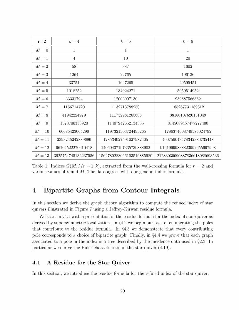
r=2 k = 4 k = 5 k = 6

M = 0 1 1 1

M = 1 4 10 20

M = 2 58 387 1602

M = 3 1264 22765 196136

M = 4 33751 1647265 29595451

M = 5 1018252 134924271 5059514952

M = 6 33331794 12003007130 939887566862

M = 7 1156714720 1132713788250 185267731189312

M = 8 41942224979 111732981265605 38180107620131049

M = 9 1573700333920 11407942652134355 8145089457477277400

M = 10 60685423064290 1197321303724493265 1786374698749585024792

M = 11 2393245242889696 128534027591027982405 400759043478342386735448

M = 12 96164522270610418 14060437197335739888902 91619999838823992655697998

M = 13 3925754745132237556 1562780288066103516885980 21283030090887836618088693536

Table 1: Indices Ω(M,Mr + 1, k), extracted from the wall-crossing formula for r = 2 andvarious values of k and M. The data agrees with our general index formula.

4 Bipartite Graphs from Contour Integrals

In this section we derive the graph theory algorithm to compute the refined index of star

quivers illustrated in Figure 7 using a Jeffrey-Kirwan residue formula.

We start in §4.1 with a presentation of the residue formula for the index of star quiver as

derived by supersymmetric localization. In §4.2 we begin our task of enumerating the poles

that contribute to the residue formula. In §4.3 we demonstrate that every contributing

pole corresponds to a choice of bipartite graph. Finally, in §4.4 we prove that each graph

associated to a pole in the index is a tree described by the incidence data used in §2.3. In

particular we derive the Euler characteristic of the star quiver (4.19).

4.1 A Residue for the Star Quiver

In this section, we introduce the residue formula for the refined index of the star quiver.

20

We begin with a recollection of the data of the star quiver and introduce the relevant

notation.

Let e denote the total rank of the gauge group of the star quiver.6 The residue formula

that we use to compute cohomology of star quivers has e integration variables (known as

gauge fugacities). We label them as follows.

• The gauge fugacities of the central non-abelian node of the star quiver are indicated

by ua, a = 1, · · · , N.

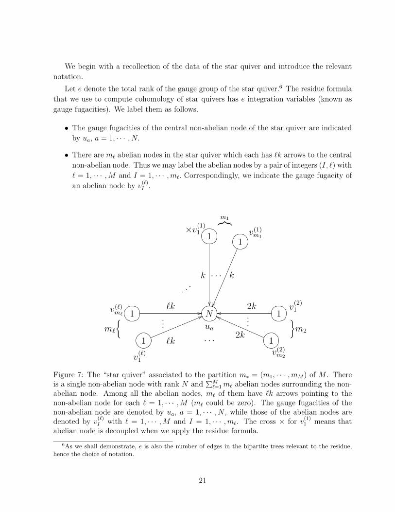
• There are m` abelian nodes in the star quiver which each has `k arrows to the central

non-abelian node. Thus we may label the abelian nodes by a pair of integers (I, `) with

` = 1, · · · ,M and I = 1, · · · ,m`. Correspondingly, we indicate the gauge fugacity of

an abelian node by v(`)I .

N1

1

1

1

11

`k

. ..

...

`k

m`

k

2k

...m2

2k

· · · k

m1︷︸︸︷

. . .

×v(1)1 v(1)

m1

v(2)m2

v(2)1

v(`)1

v(`)m`

ua

// 66

oohh

Figure 7: The “star quiver” associated to the partition m∗ = (m1, · · · ,mM) of M . Thereis a single non-abelian node with rank N and

∑M`=1m` abelian nodes surrounding the non-

abelian node. Among all the abelian nodes, m` of them have `k arrows pointing to thenon-abelian node for each ` = 1, · · · ,M (m` could be zero). The gauge fugacities of thenon-abelian node are denoted by ua, a = 1, · · · , N , while those of the abelian nodes aredenoted by v

(`)I with ` = 1, · · · ,M and I = 1, · · · ,m`. The cross × for v

(1)1 means that

abelian node is decoupled when we apply the residue formula.

6As we shall demonstrate, e is also the number of edges in the bipartite trees relevant to the residue,hence the choice of notation.

21

Next, consider the node (I, `). This node has `k identical arrows emanating from it.

As a result, the quantum mechanics has an su(`k) flavor symmetry rotating these chiral

multiplets. We may introduce fixed flavor fugacities into the contour integral.

• The flavor fugacities associated to the su(`k) flavor symmetry acting on nodes ema-

nating from the node (I, `), are denoted by ξ(I,`)i with i = 1, · · · , `k. We choose these

flavor fugacites to be generic complex numbers. In particular, this means that the

ξ(I,`)i are linearly independent over the rational numbers. Thus, any relation of the

form ∑q

(I,`)i ξ

(I,`)i = 0 , (4.1)

with rational q(I,`)i implies that all q

(I,`)i vanish.

It is important that the the refined index Ω(Mkm∗,N , y) in fact does not depend on the the

flavor fugacities due to the N = 4 supersymmetry [11]. Our purpose in introducing these

variables is to separate multiple poles in contour integrals and turn the residue calculation

into a combinatorics problem.

Finally, before introducing the residue integral, we recall an important technical point.

To compute the refined index of the quiver quantum mechanics, we must decouple a u(1)

vector multiplet; otherwise the fermionic zero modes of the overall u(1) would make the

answer zero.7 The index does not depend on which u(1) we decouple. For concreteness,

we will decouple the (I = 1, ` = 1)-th abelian node whose gauge fugacity is v(1)1 .8 In the

following, v(1)1 is interpreted to vanish when it appears in equations.

We are now prepared to introduce the residue formula for the index. According to the

general supersymmetric localization arguments of [9–11] the index may be expressed as9

Ω(Mkm∗,N , y) =

(1

sin(z)

)e ∑(u∗,v∗)∈M∗sing

JK-Res(u,v)=(u∗,v∗)

(Q(u∗, v∗), ζ)Z1-loop(u, v, z, ξ) , (4.2)

where y = eiz, and e is the rank of the star quiver after decoupling an overall U(1) :

e = N +M∑`=1

m` − 1 . (4.3)

Let us describe in detail the elements of the residue formula (4.2).

7This is due to the fact that all mater transforms in adjoints and bifundamentals, thus an overall u(1)in the gauge group, decouples.

8For partitions with vanishing m1, one must decouple an alternate choice of gauge fugacity v(`)I . As we

will ultimately see, the symmetry between the nodes, including the decoupled one, is restored. Thus, thechoice of which node one decouples is irrelevant.

9We have suppressed the dependence of Ω on the FI parameter ζ since we are only interested in thechoice (4.5).

22

• The one-loop determinant Z1-loop is10

Z1-loop(u, v, z, ξ) =1

N !

N∏a,b=1a6=b

sin(ua − ub)sin(ua − ub + z)

M∏`=1

m∏I=1

`k∏i=1

sin(ua − v(`)I − ξ(I,`)

i + z)

sin(ua − v(`)I − ξ(I,`)

i ),

(4.4)

• The FI parameter ζ ∈ Ce is determined by the MPS formula [38] to be

ζ =

1, · · · , 1︸ ︷︷ ︸N

, − 1

MN, · · · ,− 1

MN︸ ︷︷ ︸

m1−1

, − 2

MN, · · · ,− 2

MN︸ ︷︷ ︸

m2

, · · · ,− `

MN, · · · ,− `

MN︸ ︷︷ ︸

m`

, · · ·

,

(4.5)

where we order the variables as (ua, v(1)I , v

(2)I , · · · , v(`)

I , · · · , v(M)I ). Again, we only have

m1 − 1 components equal to −1/M because one of the abelian node with k arrows is

decoupled. Notice that if we had not decoupled the u(1), the sum of the components

of ζ would be N × 1N−∑`m` × `

M= 0, indicating that the overall u(1) decouples.

• The summation is over points (u∗, v∗) in the gauge fugacity space where at least e

of the sine factors appearing in the denominator of (4.4) vanish. These are poles

which may contribute to the residue extracted by the operator JK-Res. We explain

this operator in detail in the following subsection.

4.2 The Jeffrey-Kirwan Rule

In this section, we describe the residue operator JK-Res which specifies the contribution

of a given pole point (u∗, v∗) in the gauge fugacity space. We refer to the resulting rule

dictating which poles contribute to the index as the “Jeffrey-Kirwan rule”.

Consider a given polar point (u∗, v∗). This pole is said to be non-degenerate if there are

exactly e denominator factors in (4.4) which vanish at (u∗, v∗). Meanwhile, if more than e

denominator factors in (4.4) vanish at (u∗, v∗) the pole is said to be degenerate.

For general M,N , both the degenerate and non-degenerate poles contribute to the index.

However, in the case

N = Mr + 1 , (4.6)

for some non-negative integer r, only the non-degenerate poles contribute. We argue for

10We use a slightly different conventions on u and z than in [10]. uhere = πuthere and zhere = −πzthere.

23

this significant technical simplification in Appendix B. In the remainder of our analysis,

we restrict to the case where (4.6) holds. Our task is thus reduced to describing the non-

degenerate poles.

At each non-degenerate pole (u∗, v∗), there are exactly e denominator factors that vanish

at (u∗, v∗). Each such denominator factor is a sine function whose argument is a linear

function of the gauge and flavor fugacities. The dependence on the gauge fugacities is

conveniently encoded by a vector Q composed of the coefficients of the gauge fugacities

in the arguments of the sine function. A non-degenerate pole is thus associated to e such

vectors Q1, · · · , Qe. We denote the collection of these e vectors as Q(u∗, v∗).

For each non-degenerate pole, the Jeffrey-Kirwan residue operator may be conveniently

phrased in terms of the associated vectors Q(u∗, v∗). First, define the positive cone of the

vectors Q(u∗, v∗), to be those vectors that may be expressed as linear combinations of

the Qi with positive real coefficients. We denote this cone as Cone(Q(u∗, v∗)). Then, the

Jeffrey-Kirwan residue operator is

JK-Res(u,v)=(u∗,v∗)

(Q(u∗, v∗), ζ)1

Q1(u, v)· · · 1

Qe(u, v)=

det |(Q1 · · ·Qe)|−1 , ζ ∈ Cone(Q(u∗, v∗)) ,

0 , ζ /∈ Cone(Q(u∗, v∗)) .

(4.7)

Thus, to evaluate the general residue formula (4.2) we must enumerate the non-degenerate

poles with ζ ∈ Cone(Q(u∗, v∗)). To determine the full y-dependent index of the star quiver

(4.2), we then sum the resulting contributions from each pole. We carry this out explicitly

in §6. Meanwhile, in the special case of the Euler characteristic (y = 1) it is easy to see

that each pole with ζ ∈ Cone(Q(u∗, v∗)) contributes exactly 1/(Mr + 1)! to χ(Mkm∗,Mr+1).

Evaluating the Euler characteristic is therefore reduced to the combinatorial enumeration

of contributing poles.

We begin our task of tallying these poles by examining the FI parameter. In the case

N = Mr + 1 of interest this takes the form

ζ =

1, · · · , 1︸ ︷︷ ︸N

, −(r +1

M), · · · ,−(r +

1

M)︸ ︷︷ ︸

m1−1

, −(2r +2

M), · · · ,−(2r +

2

M)︸ ︷︷ ︸

m2

,

· · · , −(`r +`

M), · · · ,−(`r +

`

M)︸ ︷︷ ︸

m`

, · · ·

.

(4.8)

A contributing pole is defined by choosing e factors in the denominator of (4.4), and we

aim to constrain admissible choices.

24

First of all, it is easy to see that we can never have a contributing pole where one of the

vanishing sine factors is sin(ua − ub), as in that case the associated vector Q is orthogonal

to ζ. Next, note that when we write ζ as a positive linear combination of the Q vectors

corresponding to11 sin(ua− v(`)I − ξ(I,`)

i ) and sin(ua− ξ(1,1)i ), the coefficients are less than or

equal to 1; otherwise the components of ζ corresponding to ua would exceed 1. Examining

the coefficient of v(`)I , it then follows that we have to pick at least `r+ 1 factors of the form

sin(ua − v(`)I − ξ(I,`)

i ) for some a = 1, · · · , N and i = 1, · · · , `k.

We now show that `r + 1 is exactly the number of sines we need to pick to correctly

account for the coefficient of v(`)I . Suppose we have picked `r + 1 + δ(I,`) factors sin(ua −

v(`)I − ξ(I,`)

i ) for each (I, `) with δ(I,`) ≥ 0. We argue that δ(I,`) = 0. We must select the

remaining sine factors to be of the form sin(ua − ξ(1,1)i ). The remaining number of sine

factors to choose is

e−∑

(I,`) 6=(1,1)

(`r + 1 + δ(I,`)

)= (r + 1)−

∑(I,`)6=(1,1)

δ(I,`) . (4.9)

Now the sum of the N components corresponding to ua is

(r + 1)−∑

(I,`)6=(1,1)

δ(I,`) +∑

(I,`) 6=(1,1)

(`r +

`

M

)= Mr + 1−

∑(I,`)6=(1,1)

δ(I,`) . (4.10)

On the other hand, the sum of the components corresponding to ua for the FI parameter ζ

(4.8) is N = Mr + 1. It follows that δ(I,`) = 0.

To summarize, for each (I, `), we have to pick precisely `r + 1 sin(ua − v(`)I − ξ

(I,`)i )

factors. Meanwhile, we have to pick r+ 1 factors of the form sin(ua− ξ(1,1)i ) which we may

view as being associated to the decoupled node. This is the same number had the node not

been decoupled. We thus see that in the case N = Mr + 1, the decoupled node is treated

on the same footing as the others. This gives the Jeffrey-Kirwan rule:

JK Rule: For a given (I, `), we need to pick exactly (`r+1) factors sin(ua−v(`)I −ξ(I,`)

i )’s

in the denominator of (4.4) for the pole to make a non-zero contribution to the residue.

4.3 From Poles to Bipartite Graphs

We are now ready to enumerate all the poles satisfying the Jeffrey-Kirwan rule. It turns out

that the resulting combinatorics problem has a natural interpretation in graph theory. In

this section we describe the dictionary between a contributing pole and a bipartite graph.

11Recall that we have decoupled a node that would have had gauge fugacity v(1)1 . The factor sin(ua−ζ(1,1)i )

in Z1-loop corresponds to the chiral multiplet connected to this decoupled node.

25

We begin with the choices of the flavor fugacities ξ(I,`)i appearing in the sine factors.

Different choices of flavor fugacities will not be reflected as different bipartite graphs which

we introduce. Given a group of arrows emanating from the node (I, `), the choices for the

flavor fugacities are easy to enumerate and will be considered a trivial factor.

Indeed, the only rule for choosing the flavor fugacities is that if the ξ’s in two sine factors

are the same, then the residue for that pole is zero. For example, if we pick both

sin(u1 − v(`)I − ξ(I,`)

1 ) , sin(u2 − v(`)I − ξ(I,`)

1 ) ,

it follows that u1 = u2 at this pole. The residue for this pole is then zero due to the factor

sin2(u1 − u2) in the numerator of (4.4). Hence for each group of arrows labels by (I, `),

we have to pick `r + 1 distinct ξ (with order) out of the `k of them. This results in the

following factor

M∏`=1

[(`k

`r + 1

)(`r + 1)!

]m`

. (4.11)

Next, we must choose which ua’s are in the selected sin(ua − v(`)I − ξ) factors.12 We

represent these choices by a bipartite graph G = (VL + VR, E) with VL and VR being the

two disjoint sets of vertices and E being the set of edges.

The set of bipartite graphs of interest is G(~Lm∗,r) introduced in §2.3. For a bipartite

graph in G(~Lm∗,r), it has vL =∑`m` vertices in VL and vR = N = Mr + 1 vertices in

VR. We will label the vertex in VL by a pair of integers13 (I, `) with I = 1, · · · ,m` and

` = 1, · · · ,M . For G ∈ G(~Lm∗,r), the (I, `)-th vertex in VL is incident to `r + 1 edges. The

total number of edges e is therefore

e =M∑`=1

m`(`r + 1) = Mr +M∑`=1

m`, (4.12)

which is again the total rank of the star quiver.

We may now translate every pole for the star quiver associated to the partition m∗ into

a bipartite graph in G(~Lm∗,r),

• Each vertex in VL corresponds to a gauge fugacity v(`)I of the (I, `)-th abelian node.

• Each vertex in VR corresponds to a gauge fugacity ua of the non-abelian node.

12We will not write the superscript for the flavor fugacities from now on as the number of choices havebeen enumerated in (4.11).

13If m` = 0, then we do not have the corresponding vertex.

26

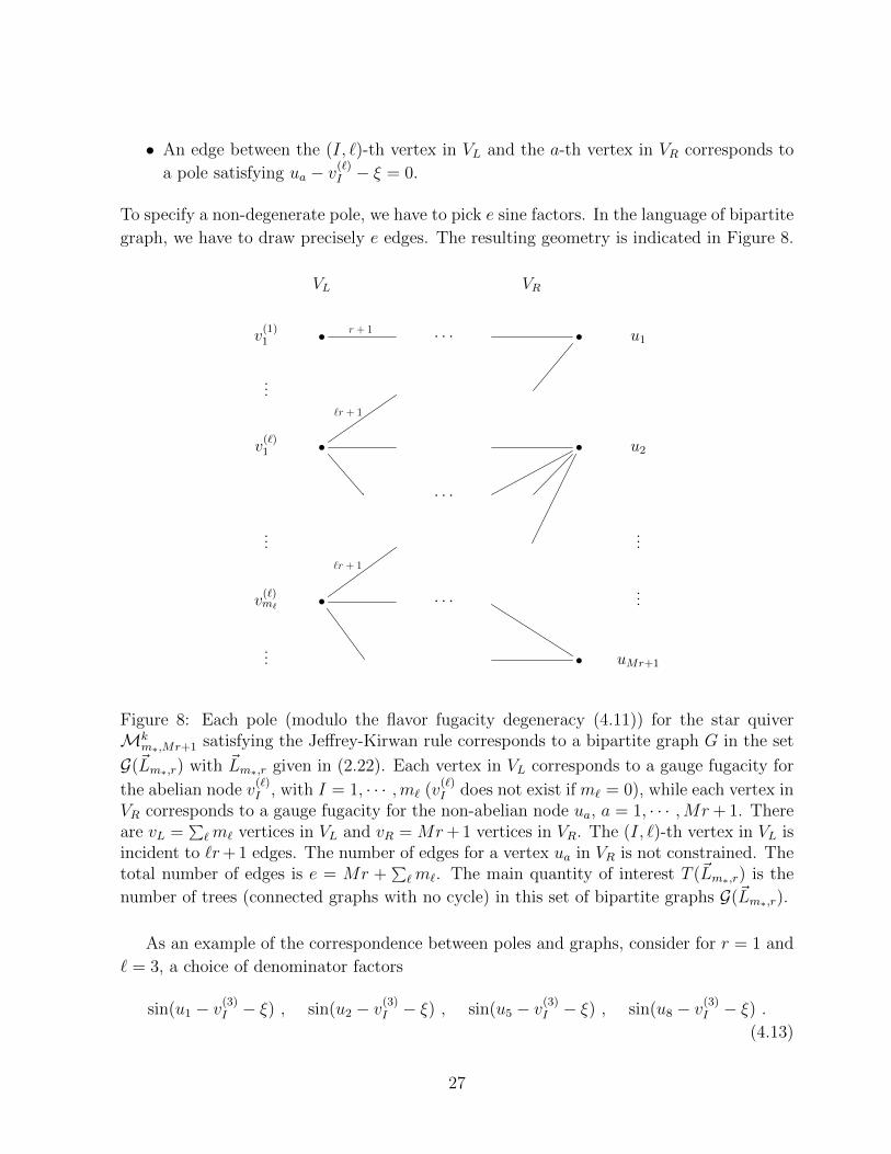
• An edge between the (I, `)-th vertex in VL and the a-th vertex in VR corresponds to

a pole satisfying ua − v(`)I − ξ = 0.

To specify a non-degenerate pole, we have to pick e sine factors. In the language of bipartite

graph, we have to draw precisely e edges. The resulting geometry is indicated in Figure 8.

VL VR

v(1)1 • r + 1 · · · • u1

...

v(`)1 •

`r + 1

• u2

· · ·

......

v(`)m` •

`r + 1

· · · ...

... • uMr+1

Figure 8: Each pole (modulo the flavor fugacity degeneracy (4.11)) for the star quiverMk

m∗,Mr+1 satisfying the Jeffrey-Kirwan rule corresponds to a bipartite graph G in the set

G(~Lm∗,r) with ~Lm∗,r given in (2.22). Each vertex in VL corresponds to a gauge fugacity for

the abelian node v(`)I , with I = 1, · · · ,m` (v

(`)I does not exist if m` = 0), while each vertex in

VR corresponds to a gauge fugacity for the non-abelian node ua, a = 1, · · · ,Mr+ 1. Thereare vL =

∑`m` vertices in VL and vR = Mr+ 1 vertices in VR. The (I, `)-th vertex in VL is

incident to `r+ 1 edges. The number of edges for a vertex ua in VR is not constrained. Thetotal number of edges is e = Mr +

∑`m`. The main quantity of interest T (~Lm∗,r) is the

number of trees (connected graphs with no cycle) in this set of bipartite graphs G(~Lm∗,r).

As an example of the correspondence between poles and graphs, consider for r = 1 and

` = 3, a choice of denominator factors

sin(u1 − v(3)I − ξ) , sin(u2 − v(3)

I − ξ) , sin(u5 − v(3)I − ξ) , sin(u8 − v(3)

I − ξ) .(4.13)

27

This corresponds to the bipartite subgraph in Figure 9. Note that we have `r+ 1 = 4 edges

incident to the vertex v(3)I .

VL VR

v(3)I • • u1

• u3

• u5

• u8

Figure 9: A bipartite subgraph corresponds to the choice of vanishing factors in (4.13).

As a more advance example, consider

r = 1, M = 4, m∗ = (m1 = 2, m2 = 1, m3 = 0, m4 = 0) . (4.14)

The number of vertices v(`)I in VL and the number of vertices ua in VR are

vL =∑`

m` = 3, vR = Mr + 1 = 5. (4.15)

There are 2 edges incident to the vertices v(1)1 and v

(1)2 and 3 edges incident to the vertex

v(2)1 . An example of poles satisfying the Jeffrey-Kirwan rule is given by the choice of sine

factors14

sin(u1 − v(1)1 − ξ) , sin(u4 − v(1)

1 − ξ) ,sin(u1 − v(1)

2 − ξ) , sin(u5 − v(1)2 − ξ) ,

sin(u1 − v(2)1 − ξ) , sin(u2 − v(2)

1 − ξ) , sin(u3 − v(2)1 − ξ) .

(4.16)

This choice corresponds to the bipartite graph in G(~Lm∗,1) in Figure 10.

4.4 From Bipartite Graphs to Poles: The Tree Rule

So far we have translated every pole (modulo the degeneracy of choosing the flavor fugacities

(4.11)) satisfying the Jeffrey-Kirwan rule into a bipartite graph in G(~Lm∗,r). However not

14As usual, v(1)1 is understood to be zero below, though we sometimes write it explicitly to make the

notation more uniform.

28

VL VR

v(1)1 • • u1

v(1)2 • • u2

v(2)1 • • u3

• u4

• u5

Figure 10: The bipartite graph corresponding to the pole in (4.16). In this example M = 4,r = 1, and the partition is m∗ = (2, 1, 0, 0). The number of vertices are vL = 3 and vR = 5.

There are 2 edges incident to the vertices v(1)1 and v

(1)2 and 3 edges incident to the vertex

v(2)1 .

every bipartite graph in G(~Lm∗,r) has an associated contributing pole in the index problem.

As we argue in this section, only those G ∈ G(~Lm∗,r) that are connected and have no cycles,

known as trees in graph theory, correspond to poles that exist. This will be referred as the

“Tree Rule”.

The essential logic may be demonstrated in a basic example. For instance, for r = 1,

the candidate pole

sin(u1 − ξ(1,1)i ) , sin(u1 − ξ(1,1)

j ) , (4.17)

for some i 6= j corresponds to the bipartite graph in Figure 11(a). At this hypothetical

pole we have u1 − ξ(1,1)i = 0 and u1 − ξ(1,1)

j = 0. However, this implies a relation among the

flavor fugacities and violates our choice of these parameters as generic complex numbers

(4.1). Thus, there is in fact no pole associated to the choice of vanishing factors (4.17).

The key observation is that the relation on the flavor fugacities arises from a cycle in the

corresponding graph.

As a more advanced example with r = 1, consider the hypothetical choice of vanishing

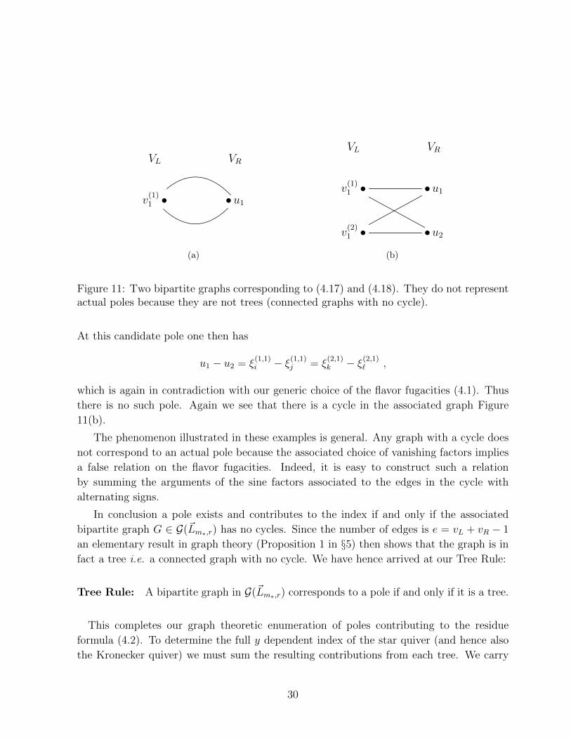
factors

sin(u1 − v(1)1 − ξ(1,1)

i ) , sin(u2 − v(1)1 − ξ(1,1)

j ) ,

sin(u1 − v(1)2 − ξ(2,1)

k ) , sin(u2 − v(1)2 − ξ(2,1)

` ) .(4.18)

29

VL VR

v(1)1 • •u1

(a)

VL VR

v(1)1 • •u1

v(2)1 • •u2

(b)

Figure 11: Two bipartite graphs corresponding to (4.17) and (4.18). They do not representactual poles because they are not trees (connected graphs with no cycle).

At this candidate pole one then has

u1 − u2 = ξ(1,1)i − ξ(1,1)

j = ξ(2,1)k − ξ(2,1)

` ,

which is again in contradiction with our generic choice of the flavor fugacities (4.1). Thus

there is no such pole. Again we see that there is a cycle in the associated graph Figure

11(b).

The phenomenon illustrated in these examples is general. Any graph with a cycle does

not correspond to an actual pole because the associated choice of vanishing factors implies

a false relation on the flavor fugacities. Indeed, it is easy to construct such a relation

by summing the arguments of the sine factors associated to the edges in the cycle with

alternating signs.

In conclusion a pole exists and contributes to the index if and only if the associated

bipartite graph G ∈ G(~Lm∗,r) has no cycles. Since the number of edges is e = vL + vR − 1

an elementary result in graph theory (Proposition 1 in §5) then shows that the graph is in

fact a tree i.e. a connected graph with no cycle. We have hence arrived at our Tree Rule:

Tree Rule: A bipartite graph in G(~Lm∗,r) corresponds to a pole if and only if it is a tree.

This completes our graph theoretic enumeration of poles contributing to the residue

formula (4.2). To determine the full y dependent index of the star quiver (and hence also

the Kronecker quiver) we must sum the resulting contributions from each tree. We carry

30

out this procedure in §6 for various examples.

In the case of the Euler characteristic, the results of this section provide more complete

information. Given a star quiver associated to the partition m∗ and a non-negative integer

r, the number of contributing poles is the number of trees in the set G(~Lm∗,r), which we

call T (~Lm∗,r). Each pole contributes to the Euler characteristic by 1/(Mr+1)!. Combining

these with the choices of flavor fugacities (4.11), we arrive at the formula

χ(Mkm∗,Mr+1) =

1

(Mr + 1)!T (~Lm∗,r)

M∏`=1

[(`k

`r + 1

)(`r + 1)!

]m`

, (4.19)

with T (~Lm∗,r) the number of trees with incidence data as described in §2.3.

5 Graph Theory

In this section we will prove the Tree Counting Theorem 1 in graph theory language.

Combined with the results of §4, this completes the derivation of our main result (2.28) for

the Euler characteristic of Kronecker moduli space.

In §5.1 we introduce necessary basic notions in graph theory. In §5.2 we define the

concept of division of a bipartite graph which crucial to our proof. Finally, in §5.3 we prove

the Tree Counting Theorem using divisions.

5.1 Generalities in Graph Theory

We begin with a review of various basic notions in graph theory. We denote the number

of vertices and edges of a graph G by v and e, respectively. All the graphs of interest are

undirected graphs (the edges are unorientated).

Definition 1 Let G be a graph consisting of vertices and edges. A trail is a sequence of

vertices and edges in G, where each edge’s endpoints are the preceding and following vertices

in the sequence. A path is a trail where no vertices (and hence edges) are repeated, except

possibly the first and the last. A cycle is a path in which the first and the last vertices are

the same.

Definition 2 Let G be a graph. G is a tree if it is connected and has no cycle.

Proposition 1 The following are equivalent for a graph G with e edges and v vertices:

• G is a tree.

31

• G is connected and e = v − 1.

• G has no cycle and e = v − 1.

Proof See, for example, Theorem 3.1.3 of [42].

The graphs of most interest for our purpose are bipartite graphs:

Definition 3 A bipartite graph is a graph whose vertices can be divided into two disjoint

sets VL and VR such that every edge connects a vertex in VL to VR. VL and VR are called

the partite sets.

We denote a bipartite graph by G = (VL + VR, E) with E being the set of edges in

the graph. We denote the number of vertices in VL and VR by vL and vR, respectively.

As before, the total number of vertices and edges are indicated by v(= vL + vR) and e,

respectively.

5.2 Division of Bipartite Graphs

In this section we develop various concepts which are useful preliminaries to the Tree

Counting Theorem 1. The main idea is called division defined below.

Definition 4 (Division) Let G = (VL + VR, E) be a bipartite graph. A division of G is

a disjoint union E = L ∪R of edges such that the following conditions hold.

• Each vertex in VL is incident to at most one edge in L (blue).

• Each vertex in VR is incident to at most one edge in R (red).

Each of L and R will be called a compartment of the division. We will put the edges in

L and R in blue and red, respectively. G is said to be divisible if it admits a division.

Remark Not every bipartite graph is divisible. See Figure 12 for a simple example.

Remark Let the numbers of edges in L and R be eL and eR, respectively. Clearly, eL (eRresp.) cannot be bigger than vL (vR resp.).

Definition 5 (Maximal division) A division E = L ∪R of G = (VL + VR, E) is said to

be left maximal if each vertex in VL is incident to exactly one edge in L, i.e. eL = vL.

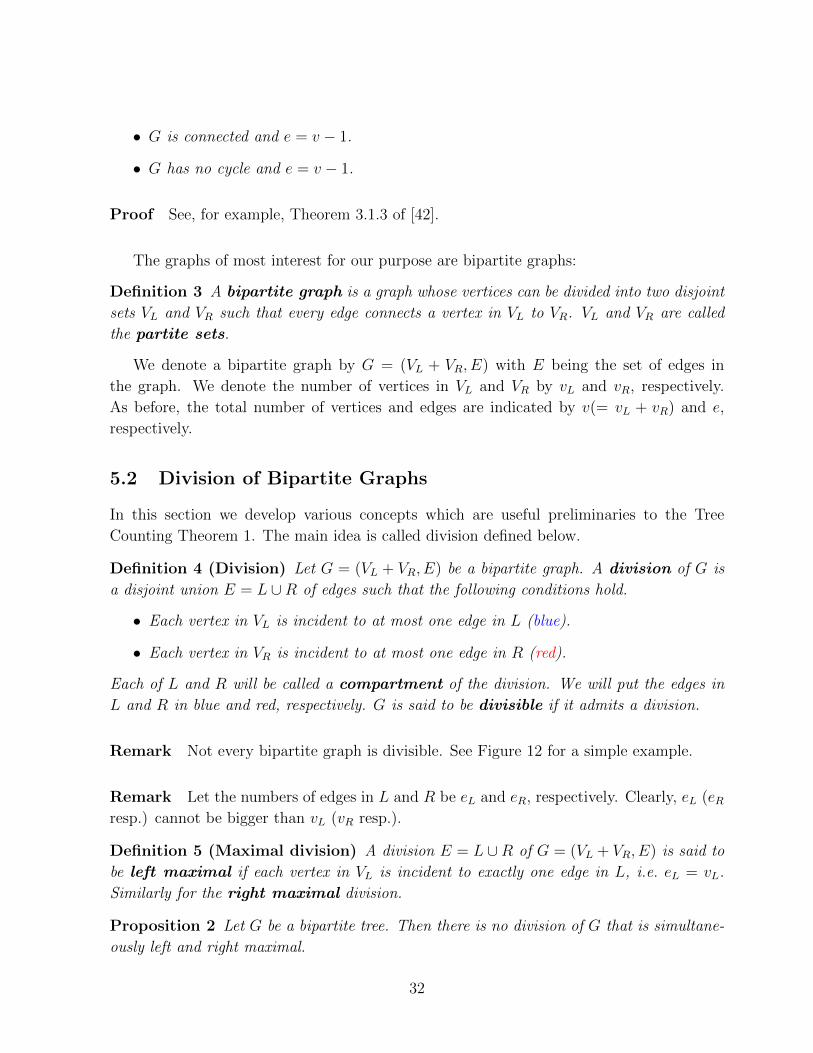
Similarly for the right maximal division.

Proposition 2 Let G be a bipartite tree. Then there is no division of G that is simultane-

ously left and right maximal.

32

VL VR

• •

Figure 12: A bipartite graph that is not divisible. If it were divisible, then two of the threeedges must belong to the same compartment, say, L. This leads to a contradiction becausethe vertex in VL is incident to two edges in L.

VL VR

• •

• •

• •

•

(a)

VL VR

• •

• •

• •

•

(b)

Figure 13: (a) An example of a division, where each vertex in VL is incident to at most oneedge in L (blue) while each vertex in VR is incident to at most one edge in R (red). (b) Anexample of a left maximal division of the same bipartite graph. In a left maximal divisionevery vertex in VL is incident to exactly one edge in the compartment L (blue).

Proof Suppose there is a simultaneous left and right maximal division of bipartite tree

G, then eL = vL and eR = vR. The total number of edges is

e = eL + eR , (5.1)

which is equal to the total number of vertices vL + vR. By Proposition 1, G cannot be a

tree, hence a contradiction.

Theorem 2 Let G = (VL+VR, E) be a tree. Then G has exactly vR left maximal divisions.

33

Proof We will prove this by explicit constructions of the vR left maximal divisions, each

of which corresponds to a vertex in VR.

Pick a vertex v in VR. Let the edges incident to v be e(1), e(2), · · · , e(Q) for some

positive integer Q. For each edge e(i), we will construct a subgraph T (i)v equipped with

a left maximal division by the following algorithm. First, color the edge e(i) in blue, i.e.

assign the edge e(i) to the compartment L. Denote the other endpoint of e(i) by v(i)1 . Since

v(i)1 is already incident to a blue edge (i.e. an edge in L), the remaining edges, if any, that

are incident to v(i)1 must be in red (i.e. belonging to R). Let us denote these red edges by

e′(i)1 , · · · , e′(i)n and the vertices in VR they are incident to by v

′(i)1 , v

′(i)2 , · · · , v′(i)n . Now for each

of the vertices v′(i)j in VR, since it is already incident to a red edge e

′(i)j , the remaining edges,

if any, that are incident to v′(i)j must be in blue. We repeat this argument and continue the

construction till the point when every terminal vertex is incident to only one edge. In this

way, for each edge e(i) incident to v, we have constructed a subtree T (i)v equipped with a

left maximal division.

Let us note the following two properties of the subtree T (i)v .

• First, the intersection of two different subtrees T (i)v consists only of the original vertex

v,

T (i)v ∩ T (j)

v = v , i 6= j . (5.2)

Suppose not, then there is another vertex v′ ∈ T (i)v ∩ T (j)

v and v′ 6= v. We can then

form a cycle passing through v and v′ in the union T (i)v ∪T (j)

v , hence contradicting the

fact that G is has no cycle.

• Second, the union of T (i)v covers the whole graph G,

G =⋃i

T (i)v , ∀ v ∈ VR . (5.3)

This follows from the fact that G is assumed to be connected, so there is a path

between v and any other point. This path must belong to one of the subtrees T (i)v by

construction.

Combining the above two properties, we see that for each vertex v ∈ VR, we can con-

struct a left maximal division of G inherited from that of T (i)v . We will denote this left

maximal division of G by E = Lv ∪Rv. Note that in E = Lv ∪Rv, v is the unique vertex in

VR that is connected to only blue lines, while each of the other vR − 1 vertices is incident

to exactly one red line. We illustrate this algorithm for two different vertices in the same

bipartite graph in Figure 14 and 15.

34

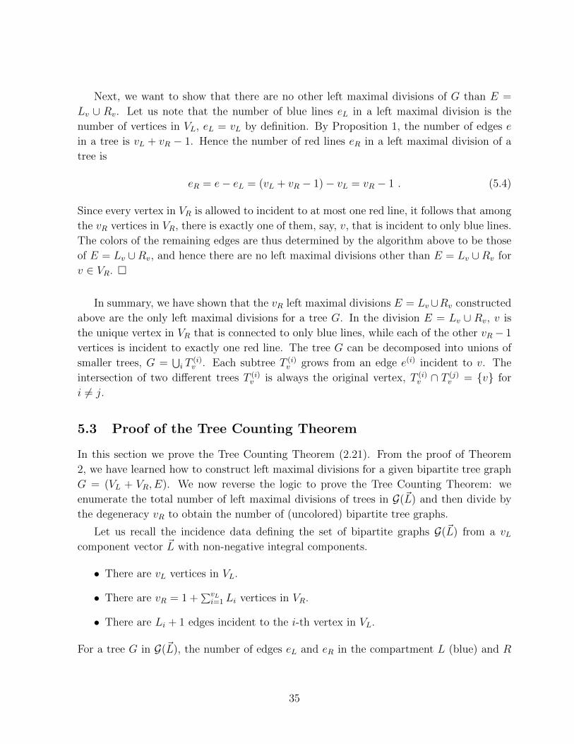
Next, we want to show that there are no other left maximal divisions of G than E =

Lv ∪ Rv. Let us note that the number of blue lines eL in a left maximal division is the

number of vertices in VL, eL = vL by definition. By Proposition 1, the number of edges e

in a tree is vL + vR − 1. Hence the number of red lines eR in a left maximal division of a

tree is

eR = e− eL = (vL + vR − 1)− vL = vR − 1 . (5.4)

Since every vertex in VR is allowed to incident to at most one red line, it follows that among

the vR vertices in VR, there is exactly one of them, say, v, that is incident to only blue lines.

The colors of the remaining edges are thus determined by the algorithm above to be those

of E = Lv ∪Rv, and hence there are no left maximal divisions other than E = Lv ∪Rv for

v ∈ VR.

In summary, we have shown that the vR left maximal divisions E = Lv∪Rv constructed

above are the only left maximal divisions for a tree G. In the division E = Lv ∪ Rv, v is

the unique vertex in VR that is connected to only blue lines, while each of the other vR − 1

vertices is incident to exactly one red line. The tree G can be decomposed into unions of

smaller trees, G =⋃i T

(i)v . Each subtree T (i)

v grows from an edge e(i) incident to v. The

intersection of two different trees T (i)v is always the original vertex, T (i)

v ∩ T (j)v = v for

i 6= j.

5.3 Proof of the Tree Counting Theorem

In this section we prove the Tree Counting Theorem (2.21). From the proof of Theorem

2, we have learned how to construct left maximal divisions for a given bipartite tree graph

G = (VL + VR, E). We now reverse the logic to prove the Tree Counting Theorem: we

enumerate the total number of left maximal divisions of trees in G(~L) and then divide by

the degeneracy vR to obtain the number of (uncolored) bipartite tree graphs.

Let us recall the incidence data defining the set of bipartite graphs G(~L) from a vLcomponent vector ~L with non-negative integral components.

• There are vL vertices in VL.

• There are vR = 1 +∑vLi=1 Li vertices in VR.

• There are Li + 1 edges incident to the i-th vertex in VL.

For a tree G in G(~L), the number of edges eL and eR in the compartment L (blue) and R

35

VL VR

• • v

• •

• •

• •

•

•

G =

=

VL VR

• oo e(1)

**

%%

• v

• •

• tt

%%

•

• •

•

•

T(1)v

+

VL VR

• • v

• tte(2)

%%

•

• •

• •

•

•

T(2)v

+

VL VR

• • v

• •

• •

•

%%

~~

e(3)

•

•

•

T(3)v

Figure 14: Construction of a left maximal division associated to the vertex v of a treeG. The graph G is further decomposed into the union of 3 subtrees T (i)

v , each of which isassociated to an edge e(i) incident to the original vertex v. v is the only vertex in VR thatis incident to only blue lines. In a left maximal division, each vertex in VL is incident toexactly one blue line, while each vertex in VR is incident to at most one red line. In additionto the above left maximal division, there are in total 6 left maximal divisions of G, each ofwhich is associated to a vertex in VR. The orientations on the edges indicate the order ofthe steps in the algorithm. The graph itself is still undirected.

VL VR

• •

• •

• •

• •

•

• v′

G =

=

VL VR

• oo

**

%%

•

• tt

%%

•

• tt

%%

•

• ee

e(1)′

>>

•

•

• v′

T(1)v′

Figure 15: Construction of a left maximal division associated to the vertex v′ of a tree G.In this case the decomposition of G is trivial, G = T

(1)v′ . In a left maximal division, each

vertex in VL is incident to exactly one blue line, while each vertex in VR is incident to atmost one red line. The orientations on the edges indicate the order of the steps in thealgorithm. The graph itself is still undirected.

36

• • 1

• • 2

• 3

• • 1

• • 2

• 3

• • 1

• • 2

• 3

Figure 16: The 3 left maximal divisions of an tree bipartite graph in G(~L), where ~L =

(1, 1) (= ~L(m1=2,m2=0),1). A bipartite graph in G(~L) has vL = 2 vertices in VL and vR = 3vertices in VR, with a total number of e = 4 edges. In a division, each vertex in VL isincident to at most one edge in L (blue) and each vertex in VR is incident to at most oneedge in R (red). In the case of left maximal division, each vertex in VL is incident to exactlyone blue edge in L.

(red) in a left maximal division E = Lv ∪Rv of G is

eL = vL , eR =vL∑i=1

Li . (5.5)

The i-th vertex in VL is incident to exactly one blue line (being left maximal) and Li red

lines.

Strategy of the Proof

We now enumerate left maximal divisions in G(~L) that are trees and thereby obtain the

number of (uncolored) trees. The procedure is outlined below:

• Step 1 Draw Li red lines from the i-th vertex in VL. Connect the∑i Li red lines to

vertices in VR, with each one of them incident to at most one red line. We refer to

the resulting graph as the red graph.

• Step 2 Draw exactly one blue line from each vertex in VL. Connect the vL blue lines

to vertices in VR such that the whole graph is connected. Up to this step we have

constructed a left maximal division of a tree in G(~L).

• Step 3 Consider all the left maximal divisions constructed above. Identify those left

maximal divisions that correspond to the same (uncolored) tree. Divide the number

of connected left maximal divisions by this degeneracy to get T (~L).

Note that by Proposition 1, in the case of e = vL + vR − 1, a graph is connected if and

only if it has no cycles. Therefore, in order to enumerate the trees, it suffices to ensure the

37

connectivity of the graph. Also note that we never generate cycles at Step 1, so it suffices

to impose the connectivity condition at Step 2.

Given a red graph GR constructed in Step 1, let the number of connected left maximal

divisions in G(~L) that contain GR be B(~L). Clearly B(~L) does not depend on the choice of

the red graph GR because every red graph has the same topology. We have the following

lemma:

Lemma 1 Given a red graph GR constructed in Step 1, the number of connected left max-

imal divisions in G(~L) that contain GR is

B(~L) = vvL−1R , (5.6)

where vR = 1 +∑vLi=1 Li. In particular, B(~L) does not depend on the choice of the red graph

GR.

Before proving this lemma, let us note that we are now ready to prove Theorem 1.

Proof of the Tree Counting Theorem

Starting from Step 1, there are eR =∑i Li red lines whereas there are vR = 1 +

∑i Li

vertices in VR, each of which is allowed to be incident to at most one red line. It follows

that exactly one vertex in VR has no red line incident to it. Hence, the number of red

graphs constructed in Step 1 is

vR(vR − 1)!∏vL

i=1 Li!, (5.7)

where vR comes from choosing which vertex in VR is left out and the multinomial coefficient(vR−1)!∏vL

i=1Li!

comes from permuting the vR − 1 red lines.

Next for Step 2, Lemma 1 instructs us to multiply the counting by a factor of B(~L) =

vvL−1R .

Finally for Step 3 we divide the counting by the degeneracy of left maximal divisions

for a given tree G ∈ G(~L), which is simply vR by Theorem 2.

Combining all these factors together, we have

T (~L) = vR(vR − 1)!∏vL

i=1 Li!︸ ︷︷ ︸Step 1

× vvL−1R︸ ︷︷ ︸

Step 2

× 1

vR︸︷︷︸Step 3

, (5.8)

where the red (blue) factors are the number of ways to draw the red (blue) lines. Hence we

have proved the Tree Counting Theorem 1.

38

Thus, to complete the argument, it remains to prove Lemma 1.

Proof of Lemma 1

It suffices to show the following claim. Let ν be a positive integer. Let L0a, L0b, L1, L2,

· · · , Lν−1 be some non-negative integers. Let I be the index set I = 0a, 0b, 1, 2, · · · , ν−1.Define

~L(1) = (L0a + L0b, L1, · · · , Lν−1)︸ ︷︷ ︸ν

, (5.9)

~L(2) = (L0a, L0b, L1, · · · , Lν−1)︸ ︷︷ ︸ν+1

. (5.10)

We will denote the sets of vertices on the left for graphs in G(~L(1)) and G(~L(2)) by V(1)L and

V(2)L , respectively. The number of vertices in V

(1)L and V

(2)L are respectively

v(1)L = ν , v

(2)L = ν + 1 . (5.11)

The number of vertices on the right in G(~L(1)) and G(~L(2)) are both

vR = 1 +∑i∈I

Li . (5.12)

We will therefore denote the sets of vertices on the right in G(~L(1)) and G(~L(2)) by the same

symbol VR without superscripts. See Figure 17 for examples of tree in G(~L1) and G(~L2).

Claim

B(~L(2)) = vRB(~L(1)) . (5.13)

Observe that this claim suffices to prove the lemma. Indeed for any ~L we have B(~L) = 1

for vL = 1.15 Thus, Lemma 1 follows immediately from the above claim by induction on

vL.

Proof of the Claim Let us label the vertices in VR by 1, 2, · · · , vR = 1 +∑i∈I Li,

VR = 1, 2, · · · , vR . (5.14)

15For vL = 1, the vector has only one component, ~L = (L1). We can choose a red graph in Step 1 to bethat each of the first L1 vertices in VR is incident to a red line while the last vertex is left out. In ordernot to have a cycle, the blue line has to be incident to the last vertex in VR, and hence B(~L) = 1.

39

For reasons that will become clear momentarily, we will label the vertices in V(1)L and V

(2)L

as

V(1)L = 0, 1, 2, · · · , ν − 1 , (5.15)

V(2)L = 0a, 0b, 1, 2, · · · , ν − 1 . (5.16)

Since B(~L) does not depend on the choice of the red graph, we will pick a convenient

red graph G(1)R in G(~L(1)) such that the first L0a + L0b vertices in VR are incident to the

vertex 0 in V(1)L , the next L1 vertices in VR are incident to the vertex 1 in V

(1)L and so on.

Similarly, we will pick a convenient red graph G(2)R in G(~L(2)) such that the first L0a vertices

in VR are incident to the vertex 0a in V(2)L , the next L0b vertices in VR are incident to the

vertex 0b in V(2)L and so on. The last vertex in VR is left out in both G

(1)R and G

(2)R . Let

Sa ⊆ VR be the set of the first L0a vertices in VR and Sb ⊆ VR be the next L0b vertices in

VR.

We will denote the set of connected (and therefore tree in this case) left maximal divisions

in G(~L(I)) that contain G(I)R as B(~L(I)), with I = 1, 2. The number of graphs in B(~L(I)) is

by definition B(~L(I)). We will label a graph b(1) in B(~L(1)) by a tuple of ν positive integers

as

b(1) = (n0, n1, · · · , nν−1) ∈ B(~L(1)) , (5.17)

meaning the vertex i in V(1)L is incident to the vertex ni in VR by a blue line. Together with

the fact that b(1) contains the red graph G(1)R , this tuple of integers uniquely determines the

left maximal division b(1). Similarly we label a graph b(2) in B(~L(2)) by a tuple of ν + 1

positive integers as

b(2) = (N0a, N0b, N1, · · · , Nν−1) ∈ B(~L(2)) . (5.18)

Note that not every choice of integers correspond to a connected graph, and therefore

does not belong to B(~L(I)). For example, we have

N0a /∈ Sa , if b(2) ∈ B(~L(2)) . (5.19)

And similarly N0b /∈ Sb if b(2) ∈ B(~L(2)). Otherwise we can form a cycle using the corre-

sponding blue line and a red line in G(2)R . Also, graphs with N0a ∈ Sb, and N0b ∈ Sa have a

cycle. We therefore have

N0a /∈ Sb or N0b /∈ Sa, if b(2) ∈ B(~L(2)). (5.20)

40

For the same reason we have

n0 /∈ Sa ∪ Sb, if b(1) ∈ B(~L(1)). (5.21)

These requirements will be important in the following.

Now define the merging map µ : B(~L(2))→ B(~L(1)) as

µ : (N0a, N0b, N1, · · · , Nν−1) 7→(n0 = N0a, n1 = N1, · · · , nν−1 = Nν−1), if N0a /∈ Sb,

(n0 = N0b, n1 = N1, · · · , nν−1 = Nν−1), if N0a ∈ Sb.(5.22)

See Figure 17 for examples of the merging map.

We need to make sure the merging map is consistent with (5.19), (5.20), and (5.21).

First note that N0a is never in Sa for b(2) ∈ B(~L(2)) by (5.19), so we do not have to worry

about hitting a point with n0 = N0a ∈ Sa, which does not belong B(~L(1)) by (5.21).

Secondly, in the case when N0a ∈ Sb, from (5.20) it follows that N0b /∈ Sa. From (5.19)

we know N0b /∈ Sb. Hence N0b /∈ Sa ∪ Sb if N0a ∈ Sb. It follows that the image graph

(n0 = N0b, n1 = N1, · · · , nν−1 = Nν−1) lies in B(~L(1)).

It is clear that the merging map µ is surjective. We now argue that µ is vR-to-1. This

then proves the claim.

Thus, fix a graph b(1) = (n0, n1, · · · , nν−1), we wish to show that its preimage consists of

exactly vR graphs. Let b(2) = (N0a, N0b, N1, · · · , Nν−1) ∈ B(~L(2)) such that µ(b(2)) = b(1).

If N0a /∈ Sb, then N0a is fixed to be n0 for µ(b(2)) = b(1), while we can freely choose

N0b ∈ VR−Sb. There are vR−L0b graphs in the preimage of this kind. On the other hand,

if N0a ∈ Sb, then N0b is fixed to be n0 for µ(b(2)) = b(1), while we can freely choose N0a to

be any point in Sb. There are L0b graphs in the preimage of this kind. Hence, given any

graph b(1) ∈ B(~L(1)), we have shown that there are vR graphs in the preimage µ−1(b(1)) .

41

B(L(2))

VL VR

0a • •Sa

0b • •Sb

•Sb

......

ν − 1• •

•

7−→

B(L(1))

VL VR

•

0 • •

•

......

ν − 1• •

•

(a)

B(L(2))

VL VR

0a • •Sa

0b • •Sb

•Sb

......

ν − 1• •

•

7−→

B(L(1))

VL VR

•

0 • •

•

......

ν − 1• •

•

(b)

Figure 17: An illustration of the merging map µ : B(L(2)) → B(L(1)). In this exampleL0a = 1 and L0b = 2. Sa only contains the first vertex in VR while Sb consists of the secondand third vertices in VR. (a) The case N0a /∈ Sb. (b) The case N0a ∈ Sb.

42

6 Computations of the Refined Index

Thus far in this work we have primarily been concerned with the degeneracy Ω(M,N, k).

In this section, we extend our analysis to the full y-dependent index Ω(M,N, k, y) whose

definition we recall here

Ω(M,N, k, y) ≡d∑p=0

y2p−d hp,p(MkM,N) , (6.1)

where d is the complex dimension of the moduli space

d = kMN −M2 −N2 + 1 . (6.2)

The y-dependent index contains much more information than the simple degeneracy

Ω(M,N, k). As a consequence, it is more challenging to determine. Nevertheless as we will

see, the residue technique described in detail in §4 can be extended to a useful algorithm

for computing the full index Ω(M,N, k, y). We present explicit formulas for small M and

N in equation (A.1).

To begin the analysis, we first note that the MPS degeneration formula can be general-

ized to include the full y dependence of the index [38]. In the case of the Kronecker quiver

with dimension vector (M,N), if we apply the MPS degeneration formula on the node M ,

we have

Ω(M,N, k, y) = y−M(M−1)−d ∑m∗`M

[M∏`=1

1

m`!

((−1)`−1

`[`]y2

)m`]ydm∗Ω(Mk

m∗,N , y) , (6.3)

where

[n]q =1− qn1− q , (6.4)

and dm∗ is the complex dimension of the moduli space for the star quiver associated to the

partition m∗ `M ,

dm∗ = kMN −M∑`=1

m` −N2 + 1 . (6.5)

We also recall that z is defined by y = eiz.

Thus, to compute the refined index Ω(M,N, k, y), it suffices to determine the refined

indices of star quivers Ω(Mkm∗,N , y). This can be carried out with the residue formula of §4.

As described there, contributing poles in the residue formula correspond to bipartite trees.

Each pole comes with an associated y-dependent contribution which we sum to determine

43

the refined index.

In the remainder of this section, we apply the formula to the Kronecker quiver with

dimension vector (2, 2r + 1) with k arrows.

6.1 Example: (2, 1)

2 Nk

// = - y2(1+y2) 1 N

2k// + 1

2 1

v u

N

1

k

k

//DD

(m1 = 0, m2 = 1) (m1 = 2, m2 = 0)

Figure 18: An example of MPS degeneration formula for M = 2. The first and thesecond quiver on the righthand side correspond to the partition (m1 = 0, m2 = 1) and(m1 = 2, m2 = 0) of M = 2, respectively.

As a gentle warmup to the more detailed calculations that follow, we begin with the

case r = 0 and dimension vector (2, 1). As discussed in §2.1.1, the moduli space is the

Grassmannian Gr(2, k) and we aim to reproduce the associated index (2.12).

There are two partitions m(1)∗ = (m1 = 0, m2 = 1) and m

(2)∗ = (m1 = 2, m2 = 0)

appearing in the degeneration formula (6.3) (see Figure 18). The quiver moduli space for

the first partition is CP2k−1 and we have

Ω(Mk

m(1)∗ ,1

, y) = y−2k+1 + y−2k+3 + · · ·+ y2k−3 + y2k−1 = y−2k+1[2k]y2 . (6.6)

For the second partition m(2)∗ in Figure 18, the integrand for the residue formula is given

by the general formula (4.4):16

(1

sin z

)2 k∏i=1

sin(u− ξ(1)i + z)

sin(u− ξ(1)i )

sin(u− v − ξ(2)i + z)

sin(u− v − ξ(2)i )

, (6.7)

where u, v stand for the gauge fugacities for the rightmost and the leftmost node in the

three-node quiver of Figure 18. The remaining node is decoupled. Meanwhile, ξ(1) and

ξ(2) are the su(k) flavor fugacities for the lower and upper group of arrows in Figure 18,

respectively. From the analysis in §4, we see that the Jeffrey-Kirwan rule instructs us to

16Here we use a slightly simplified convention on the superscripts for the gauge fugacity v and flavor

fugacities ξ’s compared with §4. To match the two conventions, we have v(1)2 = v, ξ

(I=1,`=1)i = ξ(1), and

ξ(2,1)i = ξ(2).

44

pick up one factor of sin(u− ξ(1)i ) and one factor of sin(u− v− ξ(2)

i ), and then sum over the

contributions from all such choices.

In the language of bipartite graphs, this set of poles corresponds to a single tree in

G(~Lm

(2)∗ ,0

). Recall that a bipartite graph G ∈ G(~Lm

(2)∗ ,0

) has17

vL =∑`

m` = 2 , vR = Mr + 1 = 1 , e = Mr +∑`

m` = 2 , (6.8)

where vL and vR are the number of vertices in VL and VR and e is the total number of edges

in G. The 2-dimensional vector is ~Lm

(2)∗ ,0

= (0, 0). Each vertex in VL is incident to 1 edge.

The number of trees in G(~Lm

(2)∗ ,0

) is given by the Tree Counting Theorem (2.24)

T (~Lm

(2)∗ ,0

) = 1 . (6.9)

This unique tree is illustrated in Figure 19.

VL VR

• • 1

•

Figure 19: The only tree in G(~Lm

(2)∗ ,0

), where the vector ~Lm

(2)∗ ,0

= (0, 0). In this example,

M = 2, r = 0, and m∗ = (m1 = 2, m2 = 0). The number of vertices in VL and VR arevL = 2 and vR = 1. The number of edges is e = 2. Each vertex in VL is incident to 1 edge.There is a unique tree in G(~L

m(2)∗ ,0

) corresponding to the poles u− ξ(1)i = 0, u− v− ξ(2)

j = 0

for different ξ’s.

We now sum over these poles with different choices of ξ. The resulting expression is

compactly stated in terms of variables ξ(I)mi = ξ(I)

m − ξ(I)i and the function

f(x) ≡ sin(x+ z)

sin(x). (6.10)

We find

Ω(Mk

m(2)∗ ,1

, y) =k∑

m,n=1

k∏i=1, i 6=m

f(ξ(1)mi )

k∏`=1, ` 6=n

f(ξ(2)n` ) . (6.11)

17M = 2 and r = 0 here.

45

Despite its appearance, the index (6.11) is in fact independent of the flavor fugacities ξ

due to N = 4 supersymmetry [11]. We can therefore evaluate Ω(Mk

m(2)∗ ,1

, y) in a particular

limit of ξ’s and obtain the exact answer as a function of y (or equivalently, z). We choose

the ξ’s to be purely imaginary

ξ(I)m = −iR+, I = 1, 2 , (6.12)

and further order them so that

iξ(I)1 iξ

(I)2 · · · iξ

(I)k 1 , I = 1, 2 ,

iξ(1)mm′ iξ

(2)nn′ , ∀m < m′ , n < n′ .

(6.13)

In this limit we can replace the function f(x) by the simpler expression

f(ξ(I)mm′) =

sin(ξ(I)mm′ + z)

sin(ξ(I)mm′)

→ yθ(m−m′) =

y , if m < m′ ,

y−1 , if m > m′ ,(6.14)

where θ(x) a step function

θ(x) =

+1 , if x > 0 ,

−1 , if x < 0 .(6.15)

In this limit we therefore have

k∑m=1

k∏i=1, i 6=m

f(ξ(I)mi ) = y−(k−1) + y−(k−3) + · · ·+ yk−1 = y−(k−1)[k]y2 . (6.16)

In fact, one can check that this trigonometric identity is true for arbitrary ξ’s. It follows

that the refined index for the star quiver associated to the second partition m(2)∗ is

Ω(Mk

m(2)∗ ,1

, y) = (y−(k−1)[k]y2)2 . (6.17)

Assembling the pieces using the degeneration formula (6.3), we find that the refined

index for the Kronecker quiver with dimension vector (2, 1) and k arrows is

Ω(2, 1, k, y) = y−2k+2

(− 1

2[2]y2y2k−1Ω(Mk

m(1)∗ ,1

, y) +1

2y2k−2Ω(Mk

m(2)∗ ,1

, y)

)

=y2(2−k)∏k

i=1(1− y2i)∏2i=1(1− y2i)

∏k−2i=1 (1− y2i)

.

(6.18)

46

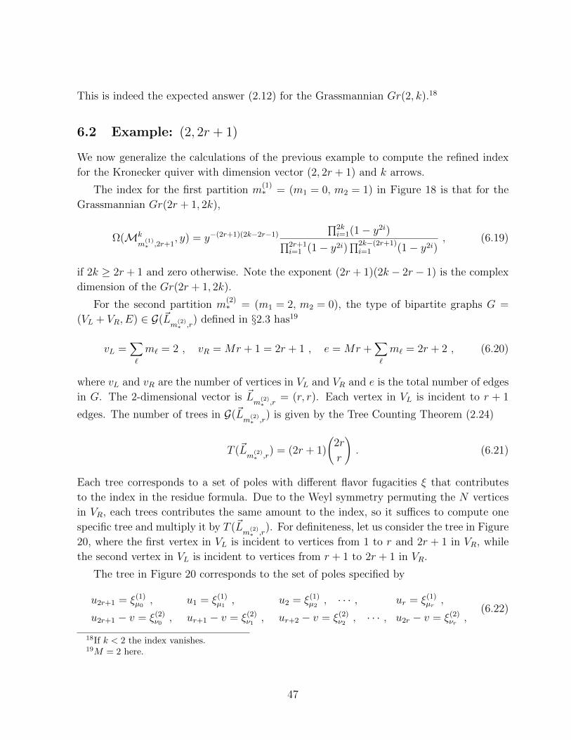
This is indeed the expected answer (2.12) for the Grassmannian Gr(2, k).18

6.2 Example: (2, 2r + 1)

We now generalize the calculations of the previous example to compute the refined index

for the Kronecker quiver with dimension vector (2, 2r + 1) and k arrows.

The index for the first partition m(1)∗ = (m1 = 0, m2 = 1) in Figure 18 is that for the

Grassmannian Gr(2r + 1, 2k),

Ω(Mk

m(1)∗ ,2r+1

, y) = y−(2r+1)(2k−2r−1)

∏2ki=1(1− y2i)∏2r+1

i=1 (1− y2i)∏2k−(2r+1)i=1 (1− y2i)

, (6.19)

if 2k ≥ 2r + 1 and zero otherwise. Note the exponent (2r + 1)(2k − 2r − 1) is the complex

dimension of the Gr(2r + 1, 2k).

For the second partition m(2)∗ = (m1 = 2, m2 = 0), the type of bipartite graphs G =

(VL + VR, E) ∈ G(~Lm

(2)∗ ,r

) defined in §2.3 has19

vL =∑`

m` = 2 , vR = Mr + 1 = 2r + 1 , e = Mr +∑`

m` = 2r + 2 , (6.20)

where vL and vR are the number of vertices in VL and VR and e is the total number of edges

in G. The 2-dimensional vector is ~Lm

(2)∗ ,r

= (r, r). Each vertex in VL is incident to r + 1

edges. The number of trees in G(~Lm

(2)∗ ,r

) is given by the Tree Counting Theorem (2.24)

T (~Lm

(2)∗ ,r

) = (2r + 1)

(2r

r

). (6.21)

Each tree corresponds to a set of poles with different flavor fugacities ξ that contributes

to the index in the residue formula. Due to the Weyl symmetry permuting the N vertices

in VR, each trees contributes the same amount to the index, so it suffices to compute one

specific tree and multiply it by T (~Lm

(2)∗ ,r

). For definiteness, let us consider the tree in Figure

20, where the first vertex in VL is incident to vertices from 1 to r and 2r + 1 in VR, while

the second vertex in VL is incident to vertices from r + 1 to 2r + 1 in VR.

The tree in Figure 20 corresponds to the set of poles specified by

u2r+1 = ξ(1)µ0

, u1 = ξ(1)µ1

, u2 = ξ(1)µ2

, · · · , ur = ξ(1)µr ,

u2r+1 − v = ξ(2)ν0

, ur+1 − v = ξ(2)ν1

, ur+2 − v = ξ(2)ν2

, · · · , u2r − v = ξ(2)νr ,

(6.22)

18If k < 2 the index vanishes.19M = 2 here.

47

VL VR

• • 1

...

• r

• r + 1

• ...

• 2r

• 2r + 1

Figure 20: A tree in G(~Lm

(2)∗ ,r

), where ~Lm

(2)∗ ,r

= (r, r). In this example, M = 2 and

m∗ = (m1 = 2, m2 = 0). The first vertex in VL is incident to vertices from 1 to r and 2r+1in VR, while the second vertex in VL is incident to vertices from r+1 to 2r+1 in VR. Thereare (2r + 1)

(2rr

)such trees, each of which corresponds to a set of poles like (6.22).

for some µ0, µ1, · · · , µr, ν0, ν1, · · · , νr = 1, · · · , k. The µ’s are all distinct and similarly for

ν’s. In the end we sum over all such µ’s and ν’s. Note that the above pole prescription

fixes

v = ξ(1)µ0− ξ(2)

ν0. (6.23)

The integrand for the Jeffrey-Kirwan residue is given by (4.4)

(1

sin(z)

)2r+2 2r+1∏a,b=1a6=b

1

f(ua − ub)k∏i=1

2r+1∏a=1

f(ua − ξ(1)i )f(ua − v − ξ(2)

i ) , (6.24)

where f(x) is defined by (6.10). The arguments of f(x) in the integrand are determined by

the position of the pole (6.22). They are

uc − ξ(1)i = ξ

(1)µci , ur+c − ξ(1)

i = ξ(1)µ0i + ξ(2)

νcν0,

uc − v − ξ(2)i = ξ(1)

µcµ0+ ξ

(2)ν0i , ur+c − v − ξ(2)

i = ξ(2)νci ,

u2r+1 − ξ(1)i = ξ

(1)µ0i , u2r+1 − ξ(2)

i = ξ(2)ν0i ,

(6.25)

where c, d = 1, 2, · · · , r (rather than to 2r + 1).

48

Since the refined index does not depend on the flavor fugacities ξ’s by the N = 4

supersymmetry, we are again free to evaluate it in the limit (6.13). In this limit f(x)f(−x) =

1, so we do not have to consider the factor∏2r+1a6=b

1f(ua−ub)

in the integrand. We can also

replace f(ξ(1)µcµ0

+ ξ(2)ν0i) by f(ξ(1)

µcµ0). The index is then

Ω(Mk

m(2)∗ ,2r+1

, y) =1

r!r!

∑(µ0, µ1, ··· , µr)

k∏i=1i 6=µ0

f(ξ(1)µ0i)

r+1

r∏c=1

k∏i=1i 6=µc

f(ξ(1)µci)

(

r∏c=1

f(ξ(1)µcµ0

)k)

×∑

(ν0, ν1, ··· , νr)

k∏i=1i 6=ν0

f(ξ(2)ν0i)

r∏c=1

k∏i=1i 6=νc

f(ξ(2)νci)

(

r∏c=1

f(ξ(2)νcν0

)

),

(6.26)

where the sum is over all tuples (µ0, µ1, · · · , µr) with distinct µ’s ranging from 1 to k.

Similarly for (ν0, ν1, · · · , νr).Using (6.14), we have

k∏i=1i 6=µa

f(ξ(1)µai) = yk−2µa+1 . (6.27)

We can then rewrite the index for the star quiver associated to m(2)∗ as

Ω(Mk

m(2)∗ ,2r+1

, y) =1

r!r!

∑(µ0, µ1, ··· , µr)

y(2r+1)(k+1)−2(r+1)µ0−2∑r

c=1µc−k

∑r

c=1θ(µc−µ0)

× ∑

(ν0, ν1, ··· , νr)

y(r+1)(k+1)−2ν0−2∑r

c=1νc−∑r

c=1θ(νc−ν0)

.

(6.28)

Again the sum is over all tuples (µ0, µ1, · · · , µr) with distinct µ’s ranging from 1 to k.

Similarly for (ν0, ν1, · · · , νr), and θ is the step function defined in (6.15).

Assembling the pieces using the degeneration formula (6.3), we arrive at our final ex-

pression for the refined index of the Kronecker quiver with dimension vector (2, 2r + 1)

Ω(2, 2r + 1, k, y) = y−2−d[− 1

2(1 + y2)ydm

(1)∗ Ω(Mk

m(1)∗ ,2r+1

, y) +1

2ydm

(2)∗ Ω(Mk

m(2)∗ ,2r+1

, y)],

(6.29)

if d = (2r+ 1)(2k− 2r− 1)− 3 ≥ 0 and zero otherwise. Here dm

(1)∗

= (2r+ 1)(2k− 2r− 1)

and dm

(2)∗

= 2k(2r + 1) − (2r + 1)2 − 1 are the ranks of the star quivers associated to

49

the partitions m(1)∗ and m

(2)∗ , respectively. Ω(Mk

m(1)∗ ,2r+1

, y) is the refined index for the

Grassmannian Gr(2j + 1, 2k) given in (6.19).

We list the first few examples of the refined index Ω(M,N, k, y) in the following:20

k = 2 :

Ω(2, 1, 2, y) = 1 ,

k = 3 :

Ω(2, 1, 3, y) =1

y2+ 1 + y2 ,

Ω(2, 3, 3, y) =1

y6+

1

y4+

3

y2+ 3 + 3y2 + y4 + y6 ,

k = 4 :

Ω(2, 1, 4, y) =1

y4+

1

y2+ 2 + y2 + y4 ,

Ω(2, 3, 4, y) =1

y12+

1

y10+

3

y8+

4

y6+

7

y4+

8

y2+ 10 + 8y2 + 7y4 + 4y6 + 3y8 + y10 + y12 ,

k = 5 :

Ω(2, 1, 5, y) =1

y6+

1

y4+

2

y2+ 2 + 2y2 + y4 + y6 ,

Ω(2, 3, 5, y) =1

y18+

1

y16+

3

y14+

4

y12+

7

y10+

9

y8+

14

y6+

16

y4+

20

y2+ 20

+ 20y2 + 16y4 + 14y6 + 9y8 + 7y10 + 4y12 + 3y14 + y16 + y18 ,

Ω(2, 5, 5, y) =1

y22+

1

y20+

3

y18+

4

y16+

8

y14+

11

y12+

17

y10+

22

y8+

30

y6+

35

y4+

41

y2+ 41

+ 41y2 + 35y4 + 30y6 + 22y8 + 17y10 + 11y12 + 8y14 + 4y16 + 3y18 + y20 + y22 .

We have checked that the above refined indices agree with [2].

Acknowledgements

We would like to thank Murad Alim, Melody Chan, Tiffany Yu-Han Chen, Yu-Wei Fan, Ben

Heidenreich, Kazuo Hosomichi, Daniel Jafferis, Cumrun Vafa, and Fan Wei for many useful

discussions. We are especially grateful to Yi-Hsiu Chen, Noam D. Elkies, Ira Gessel, Ying-

Hsuan Lin, and Alexey Ustinov for many crucial steps in the proofs. SHS is grateful for

the Kavli Institute for the Physics and Mathematics of the Universe (IPMU) and National

Taiwan University’s hospitality during the final stage of the work. The work of CC is

20For each k, the remaining cases not listed in (A.1) are redundant as a consequence of the isomorphism(3.10) Ω(2, 2r + 1, k) = Ω(2, 2(k − r − 1) + 1, k).

50

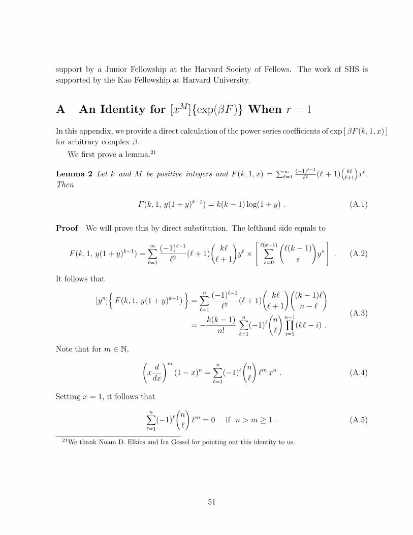
support by a Junior Fellowship at the Harvard Society of Fellows. The work of SHS is

supported by the Kao Fellowship at Harvard University.

A An Identity for [xM ]exp(βF ) When r = 1

In this appendix, we provide a direct calculation of the power series coefficients of exp [ βF (k, 1, x) ]

for arbitrary complex β.

We first prove a lemma.21

Lemma 2 Let k and M be positive integers and F (k, 1, x) =∑∞`=1

(−1)`−1

`2(` + 1)

(k``+1

)x`.

Then

F (k, 1, y(1 + y)k−1) = k(k − 1) log(1 + y) . (A.1)

Proof We will prove this by direct substitution. The lefthand side equals to

F (k, 1, y(1 + y)k−1) =∞∑`=1

(−1)`−1

`2(`+ 1)

(k`

`+ 1

)y` ×

`(k−1)∑s=0

(`(k − 1)

s

)ys

. (A.2)

It follows that

[yn]F (k, 1, y(1 + y)k−1)

=

n∑`=1

(−1)`−1

`2(`+ 1)

(k`

`+ 1

)((k − 1)`

n− `

)

= −k(k − 1)

n!

n∑`=1

(−1)`(n

`

)n−1∏i=1

(k`− i) .(A.3)

Note that for m ∈ N, (xd

dx

)m(1− x)n =

n∑`=1

(−1)`(n

`

)`m xn . (A.4)

Setting x = 1, it follows that

n∑`=1

(−1)`(n

`

)`m = 0 if n > m ≥ 1 . (A.5)

21We thank Noam D. Elkies and Ira Gessel for pointing out this identity to us.

51

Using the above identity, we see that all the higher order terms in ` in (A.3) vanish after

summing over `, and we are left with

[yn]F (k, 1, y(1 + y)k−1)

= −k(k − 1)

n!

n∑`=1

(−1)`(n

`

)n−1∏i=1

(−i)

= (−1)n−1k(k − 1)

n.

(A.6)

This concludes the proof of the lemma.

Theorem 3 Let k and M be positive integers and F (k, 1, x) =∑∞`=1

(−1)`−1

`2(` + 1)

(k``+1

)x`.

Let β be a complex number. Then

[xM ]

exp [ βF (k, 1, x) ]

=β

Mk(k − 1)

(k(k − 1)β − (k − 1)M − 1

M − 1

). (A.7)

Proof From Lemma 2, we have

exp[βF (k, 1, x)

]= (1 + y(x))βk(k−1) =

∞∑`=0

(βk(k − 1)

`

)y(x)` , (A.8)

where y(x) is defined as the solution to

x = y(1 + y)k−1. (A.9)

The Taylor series coefficient of y(x)` can be obtained by the Lagrange inversion theorem

(see, for example, [43] [44]),

y(x)` =∞∑m=0

(−1)m`

m+ `

((k − 1)(m+ `) +m− 1

m

)xm+` . (A.10)

Plugging this into (A.8), we have

[xM ]

exp [ βF (k, 1, x) ]

=1

M

M∑`=1

(−1)M−``

(βk(k − 1)

`

)(kM − `− 1

M − `

). (A.11)

Note that right-hand-sides of both (A.7) and (A.11) are polynomials in β of degree M . To

show that they are the same, it suffices to show that they have the same roots in β, while

the overall constant can be trivially checked by plugging some specific values of M,β, k.

Due to the binomial coefficient, (A.7) has zeroes at β = 0 and

β =1

k(k − 1)(kM − s) , s = 1, · · · ,M − 1 . (A.12)

52

Obviously (A.11) vanishes when β = 0. It remains to show that (A.11) vanishes when β

takes value in (A.12). When k(k − 1)β = (k − 1)M − s, (A.11) can be written as

(−1)M

M ×M !

M∑`=1

(−1)``

(M

`

)(kM − s)!

(kM − (`+ s))!

(kM − (`+ 1))!

(kM −M − 1)!(A.13)

=(−1)M

M ×M !

(kM − s)!(kM −M − 1)!

M∑`=1

(−1)`(M

`

)` (kM − (`+ 1)) · · · (kM − (`+ s− 1)) .

(A.14)

Note ` (kM − (`+ 1)) · · · (kM − (`+ s)) is a polynomial in ` of degree s. Since s < M , it

follows from (A.5) that (A.13) is zero. Thus we have shown that β = 1k(k−1)

(kM − s) with

s = 1, · · · ,M − 1 and β = 0 are roots for (A.11), which are the same M roots of (A.7).

This completes the proof.

B Degenerate Poles

In §4 we have computed the contributions to the index from the non-degenerate poles in

the residue formula (4.2). Here, we argue that the degenerate poles do not contribute when

N = Mr + 1.

Consider an integrand of the following form

sin[A(1)(u)

]· · · sin

[A(q)(u)

]sin [B(1)(u)] · · · sin [B(p)(u)]

· · · , (B.1)

where A(i)(u) and B(i)(u) are some linear functions of the gauge fugacities22 uα. The · · ·represents terms that are nonzero and finite at the pole. The index α runs over 1, · · · , e,where e is the total rank of the gauge group. Suppose at a point u = u∗, we have

A(i)(u∗) = 0 , B(i)(u∗) = 0 . (B.2)

Then u = u∗ is called a degenerate pole if p > e, and a non-degenerate pole if p = e and

q = 0. For the degenerate poles in the star quiver, we always have p − q = e, so they

are effectively simple poles after carefully “canceling” the zeroes in the numerator and the

denominator. We will be precise about this cancellation in a moment.

Let u∗ be a degenerate pole with p−q = e. As far as the residue at u = u∗ is concerned,

we can replace sin[A(i)(u)

]and sin

[B(i)(u)

]by their arguments.23 After doing so, we

22As an abuse of notations, in the general discussion here we use uα to represent both the gauge fugacities

of the non-abelian node ua and of the abelian nodes v(`)I in the star quiver (Figure 7).

23It is not, however, legitimate to replace the sine factors in · · · of (B.1) by their arguments as they do

53

perform partial fraction decomposition to break (B.1) into simple poles:

A(1)(u) · · ·A(q)(u)

B(1)(u) · · ·B(p)(u)=∑w

1

C(1,w)(u) · · ·C(e,w)(u), (B.3)

for some linear functions C(a,w)(u) of uα. Now the terms on the righthand side become

non-degenerate poles and we can evaluate their residue at u = u∗ using the technique in

§4.2. In other words, we have decomposed a degenerate pole with p − q = e into a sum of

non-degenerate poles.

In the star quiverMkm∗,N with N = Mr + 1, the degenerate poles decompose into non-

degenerate poles as described above. We claim that none of these non-degenerate poles

satisfies the Jeffrey-Kirwan rule of §4.2 and therefore they do not contribute to the index.

Let us demonstrate this claim in an explicit example. Let M = 3, r = 1, e = 6, and

m∗ = (m1 = 3, m2 = 0, m3 = 0). An example of a degenerate pole is24

u1 − v1 − ξ(1)1 = 0 , u2 − v1 − ξ(1)

1 = 0 ,

u1 − v2 − ξ(2)1 = 0 , u2 − v2 − ξ(2)

1 = 0 , u3 − v2 − ξ(2)2 = 0 ,

u1 − v3 − ξ(3)1 = 0 , u2 − v3 − ξ(3)

1 = 0 , u4 − v3 − ξ(3)2 = 0 .

(B.4)

These correspond to the p = 8 sine factors that vanish at u = u∗ in the denominator of

(B.1). Note that since u1 − v2 − ξ(2)1 = 0 and u2 − v2 − ξ(2)

1 = 0, we have u1 = u2 at this

pole. This results in q = 2 sine factors that vanish at u = u∗ in the numerator of (B.1),

sin(u1 − u2) sin(u2 − u1) . (B.5)

Note that indeed we have p− q = e.

Now performing the partial fraction decomposition, there are four terms on the right-

hand side of (B.3), each of which corresponds to a non-degenerate pole. For example, one

of them is

u1 − v1 − ξ(1)1 = 0 ,

u1 − v2 − ξ(2)1 = 0 , u3 − v2 − ξ(2)

2 = 0 ,

u1 − v3 − ξ(3)1 = 0 , u2 − v3 − ξ(3)

1 = 0 , u4 − v3 − ξ(3)2 = 0 .

(B.6)

However, this non-degenerate pole does not satisfy the Jeffrey-Kirwan rule. For example,

not vanish at u∗.24For simplicity of notation, we will denote v`=1

I simply by vI as there are no other values of ` for the

partition m∗ = (m1 = 3, m2 = 0, m3 = 0). We also abbreviate ξ(I,`=1)i by ξ

(I)i . As usual v1 = v

(1)1 is

understood to be zero since it corresponds to the decoupled abelian node.

54

there should be `r+1 = 2 sine factors with arguments ua−v1−ξ, whereas there is only one

above. It follows that this non-degenerate pole does not contribute to the index. Similarly

one can show the other three non-degenerate poles also violate the Jeffrey-Kirwan rule.

Hence the degenerate pole (B.4), which equals to the sum of four non-degenerate poles,

does not contribute to the index.

This argument may be generalized to demonstrate that in general, degenerate poles do

not contribute to the index when N = Mr + 1.

References

[1] F. Denef, “Quantum quivers and Hall / hole halos,” JHEP 0210 (2002) 023,

arXiv:hep-th/0206072 [hep-th].

[2] M. Reineke, “The Harder-Narasimhan system in quantum groups and cohomology of

quiver moduli,” Inventiones Mathematicae 152 (May, 2003) 349–368, math/0204059.

[3] M. Kontsevich and Y. Soibelman, “Stability structures, motivic Donaldson-Thomas

invariants and cluster transformations,” arXiv:0811.2435 [math.AG].

[4] M. Gross and R. Pandharipande, “Quivers, curves, and the tropical vertex,” Port.

Math. 67 no. 2, (2010) 211–259.

[5] M. Reineke, “Cohomology of quiver moduli, functional equations, and integrality of

Donaldson-Thomas type invariants,” Compos. Math. 147 no. 3, (2011) 943–964.

[6] D. Galakhov, P. Longhi, T. Mainiero, G. W. Moore, and A. Neitzke, “Wild Wall

Crossing and BPS Giants,” JHEP 1311 (2013) 046, arXiv:1305.5454 [hep-th].

[7] T. Weist, “Localization in quiver moduli spaces,” Represent. Theory 17 (2013)

382–425.

[8] T. Weist, “On the Euler characteristic of Kronecker moduli spaces,” J. Algebraic

Combin. 38 no. 3, (2013) 567–583.

[9] C. Hwang, J. Kim, S. Kim, and J. Park, “General instanton counting and 5d SCFT,”

arXiv:1406.6793 [hep-th].

[10] C. Cordova and S.-H. Shao, “An Index Formula for Supersymmetric Quantum

Mechanics,” arXiv:1406.7853 [hep-th].

[11] K. Hori, H. Kim, and P. Yi, “Witten Index and Wall Crossing,” arXiv:1407.2567

[hep-th].

55

[12] L. C. Jeffrey and F. C. Kirwan, “Localization for nonabelian group actions,” Topology

34 no. 2, (1995) 291–327. http://dx.doi.org/10.1016/0040-9383(94)00028-J.

[13] M. R. Douglas, B. Fiol, and C. Romelsberger, “Stability and BPS branes,” JHEP

0509 (2005) 006, arXiv:hep-th/0002037 [hep-th].

[14] M. R. Douglas, B. Fiol, and C. Romelsberger, “The Spectrum of BPS branes on a

noncompact Calabi-Yau,” JHEP 0509 (2005) 057, arXiv:hep-th/0003263

[hep-th].

[15] B. Fiol and M. Marino, “BPS states and algebras from quivers,” JHEP 0007 (2000)

031, arXiv:hep-th/0006189 [hep-th].

[16] B. Fiol, “The BPS spectrum of N=2 SU(N) SYM and parton branes,”

arXiv:hep-th/0012079 [hep-th].

[17] F. Denef and G. W. Moore, “Split states, entropy enigmas, holes and halos,” JHEP

1111 (2011) 129, arXiv:hep-th/0702146 [HEP-TH].

[18] M. Alim, S. Cecotti, C. Cordova, S. Espahbodi, A. Rastogi, et al., “N = 2 quantum

field theories and their BPS quivers,” Adv.Theor.Math.Phys. 18 (2014) 27–127,

arXiv:1112.3984 [hep-th].

[19] J. Manschot, B. Pioline, and A. Sen, “From Black Holes to Quivers,” JHEP 1211

(2012) 023, arXiv:1207.2230 [hep-th].

[20] S. Cecotti and M. Del Zotto, “Half-Hypers and Quivers,” JHEP 1209 (2012) 135,

arXiv:1207.2275 [hep-th].

[21] W.-y. Chuang, D.-E. Diaconescu, J. Manschot, G. W. Moore, and Y. Soibelman,

“Geometric engineering of (framed) BPS states,” arXiv:1301.3065 [hep-th].

[22] C. Cordova and A. Neitzke, “Line Defects, Tropicalization, and Multi-Centered

Quiver Quantum Mechanics,” JHEP 1409 (2014) 099, arXiv:1308.6829 [hep-th].

[23] C. Cordova, “Regge Trajectories in N = 2 Supersymmetric Yang-Mills Theory,”

arXiv:1502.02211 [hep-th].

[24] C. Cordova and S.-H. Shao, “Asymptotics of BPS Degeneracies in Quiver Quantum

Mechanics,” To Appear (2015) .

[25] T. Mainiero, “Algebraicity and Asymptotics,” To Appear (2015) .

[26] P. C. Argyres and M. R. Douglas, “New phenomena in SU(3) supersymmetric gauge

theory,” Nucl.Phys. B448 (1995) 93–126, arXiv:hep-th/9505062 [hep-th].

56

[27] D. Gaiotto, G. W. Moore, and A. Neitzke, “Wall-crossing, Hitchin Systems, and the

WKB Approximation,” arXiv:0907.3987 [hep-th].

[28] M. Alim, S. Cecotti, C. Cordova, S. Espahbodi, A. Rastogi, et al., “BPS Quivers and

Spectra of Complete N=2 Quantum Field Theories,” Commun.Math.Phys. 323

(2013) 1185–1227, arXiv:1109.4941 [hep-th].

[29] N. Seiberg and E. Witten, “Electric - magnetic duality, monopole condensation, and

confinement in N=2 supersymmetric Yang-Mills theory,” Nucl.Phys. B426 (1994)

19–52, arXiv:hep-th/9407087 [hep-th].

[30] R. Gopakumar and C. Vafa, “M theory and topological strings. 1.,”

arXiv:hep-th/9809187 [hep-th].

[31] R. Gopakumar and C. Vafa, “M theory and topological strings. 2.,”

arXiv:hep-th/9812127 [hep-th].

[32] F. Denef, “Supergravity flows and D-brane stability,” JHEP 0008 (2000) 050,

arXiv:hep-th/0005049 [hep-th].

[33] F. Denef, “On the correspondence between D-branes and stationary supergravity

solutions of type II Calabi-Yau compactifications,” arXiv:hep-th/0010222

[hep-th].

[34] P. Gabriel, “Unzerlegbare Darstellungen. I,” Manuscripta Math. 6 (1972) 71–103;

correction, ibid. 6 (1972), 309.

[35] I. N. Bernsteın, I. M. Gel’fand, and V. A. Ponomarev, “Coxeter functors, and

Gabriel’s theorem,” Uspehi Mat. Nauk 28 no. 2(170), (1973) 19–33.

[36] D. Gaiotto, G. W. Moore, and A. Neitzke, “Framed BPS States,” arXiv:1006.0146

[hep-th].

[37] M. Del Zotto and A. Sen, “About the Absence of Exotics and the Coulomb Branch

Formula,” arXiv:1409.5442 [hep-th].

[38] J. Manschot, B. Pioline, and A. Sen, “Wall Crossing from Boltzmann Black Hole

Halos,” JHEP 1107 (2011) 059, arXiv:1011.1258 [hep-th].

[39] M. Reineke, J. Stoppa, and T. Weist, “MPS degeneration formula for quiver moduli

and refined GW/Kronecker correspondence,” arXiv:1110.4847 [math.AG].

[40] R. Stanley, Enumerative Combinatorics, Volume II. Cambridge Studies in Advanced

Mathematics. Cambridge University Press, 2001.

57

[41] R. L. Graham, D. E. Knuth, and O. Patashnik, Concrete Mathematics: A

Foundation for Computer Science. Addison-Wesley Longman Publishing Co., Inc.,

Boston, MA, USA, 2nd ed., 1994.

[42] R. Gould, Graph Theory. Dover Publications, Inc., 2012.

[43] N. D. Elkies, “The power series for the inverse function of y(1− y)t,”.

http://www.math.harvard.edu/~elkies/Misc/catalan.pdf.

[44] N. D. Elkies, “Yet another proof of the series in x for the powers yβ of the solution of

y(1− y)t = x,”. http://www.math.harvard.edu/~elkies/Misc/catalan2.pdf.

58