coupled feature learning for multimodal medical image fusion
TRANSCRIPT
1
Coupled Feature Learning for Multimodal MedicalImage Fusion
Farshad G. Veshki, Student Member, IEEE, Nora Ouzir, Member, IEEE, Sergiy A. Vorobyov, Fellow, IEEE, andEsa Ollila, Senior Member, IEEE
Abstract—Multimodal image fusion aims to combine relevantinformation from images acquired with different sensors. Inmedical imaging, fused images play an essential role in bothstandard and automated diagnosis. In this paper, we proposea novel multimodal image fusion method based on coupleddictionary learning. The proposed method is general and canbe employed for different medical imaging modalities. Unlikemany current medical fusion methods, the proposed approachdoes not suffer from intensity attenuation nor loss of criticalinformation. Specifically, the images to be fused are decomposedinto coupled and independent components estimated using sparserepresentations with identical supports and a Pearson correlationconstraint, respectively. An alternating minimization algorithm isdesigned to solve the resulting optimization problem. The finalfusion step uses the max-absolute-value rule. Experiments areconducted using various pairs of multimodal inputs, includingreal MR-CT and MR-PET images. The resulting performanceand execution times show the competitiveness of the proposedmethod in comparison with state-of-the-art medical image fusionmethods.
Index Terms—Multi-modal medical imaging, image fusion,coupled dictionary learning, MRI-PET, MRI-SPECT, MRI-CT.
I. INTRODUCTION
MEDICAL imaging techniques are designed to capturespecific types of tissues and structures inside the body.
Anatomical imaging techniques can provide high-resolutionimages of internal organs. For example, magnetic resonance(MR) imaging shows soft tissues, such as fat and liquid,while computed tomography (CT) captures more effectivelyhard tissues, such as bones and implants. Functional imagingtechniques measure the biological activity of specific regionsinside the organs. Single-photon emission computed tomogra-phy (SPECT) and positron emission tomography (PET) aretypical examples of this type of techniques. The goal ofmultimodal image fusion is to combine this variety of (oftencomplementary) information into a single image. In additionto easing the visualisation of multiple images, fusion enablesa joint analysis providing relevant and new information aboutthe patient, for both traditional and automated diagnosis [1]–[3].
Medical image fusion methods mostly rely on the extractionof different types of features in the images before selecting orcombining the most relevant ones. One way of achieving this
Farshad G. Veshki, S. A. Vorobyov and Esa Ollila are withthe Department of Signal Processing and Acoustics, Aalto Univer-sity, Espoo, Finland. Nora Ouzir is with Department of Mathe-matics, CentraleSupelec, France (e-mail: [email protected];[email protected]; [email protected]; [email protected]).Corresponding author: S. A. Vorobyov.
is by transforming the images into a domain where the relevantfeatures would arise naturally. A common approach employsmulti-scale transformation (MST) techniques to extract fea-tures from different levels of resolution and select them usingan appropriate fusion rule in a subsequent step [4]–[10]. Thefinal fused image is obtained by applying the inverse MSTto the combined multi-scale features. For example, a recentMST-based fusion method using a non-subsampled shearlettransform (NSST) has been proposed in [4]. The fusion ruleis based on a pulse coupled neural network (PCNN), weightedlocal energy and a modified Laplacian [4]. In a different study,the MST is based on local Laplacian filtering (LLF), and thefusion rule relies on the information of interest (IOI) criterion[8].
Another approach seeks to learn the relevant features fromthe images. The methods that follow this approach mainlyuse sparse representations (SR) and dictionary learning [11]–[17]. First, dictionaries are learnt and used to find an SRof the images. The resulting sparse codes from both inputimages are then selected by measuring their respective levelsof activity (e.g., using the `1−norm). Once the combinedSR is obtained, the fused image is reconstructed again usingthe learnt dictionaries. In this category of methods, differentstrategies have been proposed to deal with the presence ofdrastically different components in the images. For example,the images are separated into base and detail componentsprior to the dictionary learning phase in [11]. In [12], [13],morphological characteristics, such as cartoon and texturecomponents, are used.
The multi-component strategy is useful for both SR andMST-based fusion. It allows the different layers of informationto be identified before extracting the relevant (multi-level)features, and thus reduces the loss of contrast or image quality.Many works have shown the superiority of this approach com-pared to using a single layer or component in each image [4],[8], [9], [14]. However, the choice of the multi-componentmodel is not straightforward because all decompositions donot necessarily yield features that are suitable for fusion. Forexample, in the MST approach, the highest resolution levelof MR-CT images usually depicts tissues with very differentcharacteristics, i.e., soft tissues in MR and hard structuresin CT. Fusing soft and hard tissues (using binary selection,for example) can cause a loss of useful information. Usingaveraging techniques can mitigate this loss, but it leads to anattenuation of the original intensities (particularly when thereis a weak signal in one of the input images). More generally,it is not always meaningful to apply a fusion rule when there
arX
iv:2
102.
0864
1v1
[cs
.CV
] 1
7 Fe
b 20
21

2
is no guarantee features with the same levels of resolutionencompass the same type of information. Conversely, differentimaging techniques can provide varying resolutions for thesame underlying structures. Finally, it is not always clear inpractice how to choose the number of resolution levels forMST or an adequate basis for the SR-approach.
This paper presents a novel multi-modal image fusionmethod using an SR-based multi-component approach. Ageneral decomposition model enables us to preserve theimportant features in both input modalities and reduce theloss of essential information. Specifically, coupled dictionarylearning (CDL) is used to learn features from input imagesand simultaneously decompose them into correlated and in-dependent components. The core idea of the proposed modelis that the independent components contain modality-specificinformation that should appear in the final fused image.Therefore, these components should be preserved entirelyrather than subjected to some fusion rule. Since the inputimages still represent the same anatomical region or organ,they can contain a significant amount of similar or overlappinginformation. This information is taken into account in thecorrelated components and considered relevant for fusion. Thecoupled dictionaries play a key role here; each couple of atomsrepresent a correlated feature. This allows us to choose the bestcandidate for fusion based on the most significant dictionaryatom without any loss of information. A summary of theproposed methodology and contributions is provided in thefollowing
• We employ a general decomposition model suitable forfusing images from various medical imaging modalities.
• A CDL method based on simultaneous sparse approxi-mation is proposed for estimating the correlated features.In order to incorporate variability in the appearance ofcorrelated features, we relax the assumption of equal SRsby assuming common supports only.
• The independent components are estimated using a Pear-son correlation-based constraint (enforcing low correla-tion).
• An alternating optimization method is designed for simul-taneous dictionary learning and image decomposition.
• The final fusion step combines direct summation with themax-absolute-value rule.
A thorough experimental comparison with current medicalimage fusion methods is conducted using multiple pairs of realmultimodal images. The data comprises six different combina-tions of medical imaging techniques, including MR-CT, MR-PET and MR-SPECT. The experimental results show that theproposed method results in a better fusion of local intensityand texture information, compared to other current techniques.In particular, isolating modality-specific information reducesthe loss of information significantly.
Notations: Throughout the paper, we use bold capital lettersfor matrices. A matrix with a single subscript always denotes acolumn of that matrix. For example [D1]i is the i−th columnof D1. In a matrix, the entry at the intersection of ith row andjth column is denoted as [·](i,j). In addition, the Frobeniusnorm of a matrix is denoted by ‖ · ‖F , the Euclidean normof a vector is denoted by ‖ · ‖2, and ‖ · ‖0 is the operator
counting the number of nonzero coefficients of a vector. Thesupp{·} denotes the support of a matrix. Operator | · | denotesthe absolute value of a number. The symbol (·)T denotes thetranspose operation and (·)+ stands for the updated variable.The symbol ⊥⊥ denotes the conditional independence betweentwo variables.
The remainder of the paper is organised as follows. Sec-tion II presents the proposed CDL approach and SR withcommon supports. The proposed image decomposition methodand the fusion step are explained in Section III and IV,respectively. Section V reports the experimental results usingvarious examples multi-modal images. Finally, conclusions areprovided in Section VI.
II. COUPLED FEATURE LEARNING
The objective of CDL is to learn a pair of dictionariesD1 and D2, used to jointly represent two datasets X1 andX2. The underlying relationship between these datasets iscaptured using a common sparse coding matrix A. A standardformulation of the CDL problem is given by the followingminimization problem
minD1,D2,A
‖D1A−X1‖2F + ‖D2A−X2‖2F
s.t. ‖Ai‖0 ≤ T, ‖[D1]t‖2 = 1, ‖[D2]t‖2 = 1, ∀t, i (1)
where T is the maximum number of non-zero coefficients ineach column of the sparse coding matrix A. The constraint onthe norm of the dictionary elements is used to avoid scalingambiguities. CDL is particularly suitable for tackling problemsthat involve image reconstruction in different feature spaces.The standard problem (1) has been successfully employed innumerous image processing applications, such as image super-resolution [18], single-modal image fusion [19], or photo andsketch mapping [20]. In this section, the objective is to learnthe correlated features in two input multi-modal images. Thesefeatures are captured by the atoms of the learnt dictionariesD1 and D2. Since we are dealing with images acquired fromdifferent sensors, different aspects of the same underlyingstructure can be displayed with different levels of visibilityin each modality. For example, both CT and MRI can showtendons, but they are more visible in MR images [21].We incorporate this aspect by imposing identical supportsinstead of enforcing an equal sparse representation for eachpair of dictionary atoms. In this way, correlated elementscan be represented with different levels of significance ineach dictionary. The proposed modified CDL problem can beformulated as follows
minimizeD1,D2,A1,A2
‖D1A1 −X1‖2F + ‖D2A2 −X2‖2F
s.t. supp{A1} = supp{A2}‖[A1]i‖0 ≤ T, ‖[A2]i‖0 ≤ T, ∀i‖[D1]t‖2 = 1, ‖[D2]t‖2 = 1,∀t.
(2)
Problem (1) is typically solved by alternating between asparse coding stage and a dictionary update step [22]–[24].In this work, we solve problem (2) using an alternatingapproach too. Specifically, after splitting the variables into

3
two subsets {A1,A2} and {D1,D2}, we alternate betweentwo optimization phases detailed in the following subsections.
A. Sparse Coding
Minimizing (2) with respect to the first set of variables{A1,A2} requires some changes to the standard sparse codingprocedure (e.g., OMP [25]). First, one has to enforce commonsupports. The method of simultaneous orthogonal matchingpursuit (SOMP) [26] is of interest here as it includes a commonsupport constraint. Secondly, one has to consider coupleddictionaries. This can be achieved by modifying the atomselection rule of SOMP so that each of the input signals isapproximated using a different dictionary instead of sharing asingle one. In each iteration, this modified algorithm selects apair of coupled atoms that minimizes the sum of the residualerrors, i.e.,
argmaxt|rT1 [D1]t|+ |rT2 [D2]t|
where r1 and r2 are the approximation residuals of a pair ofinput signals (e.g., r1 = [X1]i −D1[A1]i and r2 = [X2]i −D2[A2]i are the residuals corresponding to the ith columns ofX1 andX2, respectively). The optimal nonzero coefficients ofthe sparse codes are then computed based on their associatedselected atoms. As opposed to SOMP, we stop the algorithmwhen only one of the input signals meets the stopping criterion(i.e., the Euclidean norm of one of the residuals is smallerthan a user-defined threshold ε). This is based on the fact thatthe main objective of the algorithm is to estimate correlatedfeatures, whereas any remaining noise (once the approximationof one of the signals is complete) is evidently uncorrelatedwith the residual of the second signal.
B. Dictionary Update
The first two terms of (2) are independent with respect tothe dictionaries D1 and D2. They are also independent withrespect to the non-zero coefficients in A1 and A2 when thesupports are fixed. Therefore, the dictionaries D1 and D2 canbe updated individually using any efficient dictionary learningalgorithm. We choose to use the K-SVD method [22] becauseit updates the dictionary atoms and the associated sparsecoefficients without changing their supports. Specifically, K-SVD uses a singular value decomposition.
The proposed CDL method alternates between the sparsecoding step using the modified SOMP and the dictionary up-date using K-SVD. We will refer to the proposed approach asthe simultaneous coupled dictionary learning (SCDL). Fig. 1shows how the proposed SCDL method captures correlatedfeatures more efficiently than the standard CDL method of[27]. Specifically, one can see how the dictionaries obtainedusing the standard method (Fig. 1(c,d)) contain atoms thatare relatively uncorrelated (framed in red), while all theatoms obtained with SCDL present a clear correlation (seeFig. 1(a,b)).
(a) (b)
(c) (d)
Fig. 1: Example of coupled dictionaries learnt from MR (left)and CT (right) images using the proposed method (a,b) and thestandard CDL approach of [27] (c,d). The red frames indicateweakly correlated atoms.
III. IMAGE DECOMPOSITION VIA SCDL
Our fusion method relies on the decomposition of the inputimages into correlated and independent components. The latterrepresent features that are unique to each modality and thatwe seek to preserve. This section introduces the proposeddecomposition model and explains how to solve the resultingminimization problem.
A. Decomposition Model
Let the input images to be fused be denoted by I1 ∈ RM×N
and I2 ∈ RM×N .1 The correlated components are denotedby Iz1 ∈ RM×N and Iz2 ∈ RM×N , and the independentcomponents by Ie1 ∈ RM×N and Ie2 ∈ RM×N . The proposeddecomposition model can be expressed as follows{
I1 = Iz1 + Ie1
I2 = Iz2 + Ie2
where Ie1 ⊥⊥ Ie2. (3)
The SCDL method explained in Section II operates patch-wise.Therefore, we rewrite (3) using the matrices containing all theextracted patches as follows{
X1 = Z1 +E1
X2 = Z2 +E2where E1 ⊥⊥ E2, (4)
where the matrices X1 ∈ Rm×p and X2 ∈ Rm×p contain thep vectorized overlapping patches of size m extracted from theinput images. The patches of the correlated components arerepresented by Z1 ∈ Rm×p and Z2 ∈ Rm×p, and those of theindependent components by E1 ∈ Rm×p and E2 ∈ Rm×p.Fig. 2 shows how the proposed decomposition model captures
1The images are registered beforehand, which is a typical assumption inthe literature [4].

4
(a) I1 (MR) (b) Iz1 (c) Ie
1 (d) I1 − Iz1 − Ie
1
(e) I2 (CT) (f) Iz2 (g) Ie
2 (h) I2 − Iz2 − Ie
2
Fig. 2: A pair of MR and CT input images (a,e) decomposed into their coupled (b,f) and independent (c,g) components basedon the proposed model. The residuals are shown in (d,h).
correlated and independent features in a pair of MR-CT im-ages. The independent components contain edges and detailsthat can be clearly observed in only one of the modalities,e.g., sulci details in the MR image and calcification in the CTimage (indicated by red arrows). The correlated componentsrepresent the underlying joint structure that can be referred toas the base or background layer. Fig. 3, shows another exampleof decomposition for a pair of PET-MR images. In functional-anatomical imaging, any details in the images are naturallyindependent. The independent components also capture anynon-overlapping regions. Finally, the correlated componentscontain the regions where the background of the anatomicalimage overlaps with the biological activity information.
B. Minimization Problem
In order to estimate the correlated and independent com-ponents in (4), we formulate a minimization problem basedon the SCDL approach described in the previous section.Specifically, we seek the coupled sparse representation of Z1
and Z2 using sparse codes with identical supports A1 ∈ Rn×pand A2 ∈ Rn×p and coupled dictionaries D1 ∈ Rm×n andD2 ∈ Rm×n (i.e., Z1 = D1A1 and Z2 = D2A2). Theelement-wise independence of E1 and E2 is enforced byminimizing the squared Pearson correlation coefficients, wherethe local means µ and standard deviations σ are estimatedpatch-wise. The corresponding cost function is expressed asfollows
φ([E1](i,j),[E2](i,j)
)=
(([E1](i,j)−µ1,j)([E2](i,j)−µ2,j)
σ1,jσ2,j
)2
where j is the patch index and the subscripts 1 and 2 indicatethe associated components E1 and E2. Note that this patch-wise approach results implicitly in multiple counts of the same
pixel when considering overlapping patches [28]. Combiningthe independence term with the proposed SCDL approachleads to the following minimization problem
minimizeD1,D2,A1,A2,
E1,E2
∑i=1,...,mj=1,...,p
φ([E1](i,j), [E2](i,j)
)s.t. D1A1 +E1 =X1
D2A2 +E2 =X2
supp{A1} = supp{A2}‖[A1]i‖0 ≤ T, ‖[A2]i‖0 ≤ T, ∀i‖[D1]t‖2 = 1, ‖[D2]t‖2 = 1,∀t,
(5)
where the sparsity and common support constraints have beenintroduced in (2).
C. Optimization
Problem (5) is challenging because of its non-convexityand the presence of multiple sets of variables. Therefore,we propose to break the optimization procedure into simplersubproblems where we consider minimization with respect toseparate blocks of variables. We then alternate between thesesubproblems until finding a local optimum. Specifically, theminimization with respect to the sparse codes and dictionaries,and the minimization with respect to the independent com-ponents are treated separately. Furthermore, we simplify theproblem by approximating the first two equality constraintsin (5) by quadratic approximation terms. This leads to a new

5
(a) I1 (PET) (b) Iz1 (c) Ie
1 (d) I1 − Iz1 − Ie
1
(e) I2 (MR) (f) Iz2 (g) Ie
2 (h) I2 − Iz2 − Ie
2
Fig. 3: A pair of PET and MR input images (a,e) decomposed into their coupled (b,f) and independent (c,g) componentsusing the proposed model. The residuals are shown in (d,h). (The grey-scale component of the PET image is used in thedecomposition, as explained in Subsection IV-C.)
optimization problem that can be written as
minimizeD1,D2,A1,A2,
E1,E2
∑i=1,...,mj=1,...,p
φ([E1](i,j), [E2](i,j)
)+ρ
2
∑k=1,2
‖DkAk +Ek −Xk‖2F
s.t. supp{A1} = supp{A2}‖[A1]i‖0 ≤ T, ‖[A2]i‖0 ≤ T, ∀i‖[D1]t‖2 = 1, ‖[D2]t‖2 = 1,∀t
(6)
where ρ > 0 controls the trade-off between the independenceof E1 and E2 and the accuracy of the sparse representations.As mentioned above, problem (6) is tackled by alternatingminimizations with respect to the two blocks of variables{A1,A2,D1,D2} and {E1, E2}. Each resulting subproblemis described in more detail in the following.
1) Optimization with respect to {A1,A2,D1,D2}: Thefirst optimization subproblem can be written as
minimizeD1,D2,A1,A2
‖D1A1 −X′
1‖2F + ‖D2A2 −X′
2‖2F
s.t. supp{A1} = supp{A2}‖[A1]i‖0 ≤ T, ‖[A2]i‖0 ≤ T, ∀i‖[D1]t‖2 = 1, ‖[D2]t‖2 = 1,∀t
where X′
1 =X1−E1 and X′
2 =X2−E2. This subproblemis addressed using the SCDL method explained in Section II.The dictionaries can be initialized in the first iteration of thealgorithm using a predefined dictionary, e.g., based on discretecosine transforms (DCT). In subsequent iterations, the SCDLmethod is initialized using the dictionaries obtained from theprevious one. Furthermore, initializing the sparsity parameterT with a small value and gradually increasing it at eachiteration ensures a warm start of the algorithm.
2) Optimization with respect to {E1,E2}: The secondoptimization subproblem can be written as
minimizeE1,E2
∑i=1,...,mj=1,...,p
φ([E1](i,j), [E2](i,j)
)+ρ
2
∑k=1,2
‖DkAk +Ek −Xk‖2F . (7)
The estimates of {E1,E2} depend on the patch-wise meansand standard deviations, which in turn depend on the inde-pendent components themselves. Therefore, we propose toaddress this subproblem using an expectation-maximization(EM) method. The EM approach leads to the following updatesfor the independent components
[E1]+(i,j)=
ρ[X1−D1A1](i,j)+2([E2](i,j)−µ2,j)
2
max(σ21,jσ
22,j ,δ)
µ1,j
ρ+ 2([E2](i,j)−µ2,j)2
max(σ21,jσ
22,j ,δ)
[E2]+(i,j)=
ρ[X2−D2A2](i,j)+2([E1](i,j)−µ1,j)
2
max(σ21,jσ
22,j ,δ)
µ2,j
ρ+ 2([E1](i,j)−µ1,j)2
max(σ21,jσ
22,j ,δ)
where the means and standard deviations are computed usingthe current values of {E1,E2}, with δ > 0 a constant used toavoid division by zero. Note that {E1,E2} can be initializedwith zero matrices.
D. Computational Complexity
The computational cost of the proposed decompositionalgorithm is dominated by the first subproblem (solved usingSCDL). In particular, the complexity of one SCDL iteration(including all substeps) is O(pmax(Tnm, T 2m,T 3, nm2)),while the complexity of the EM step is only O(mp). Based

6
on the experimental findings of [29] and [12], sparse approxi-mations are performed in this work in single precision, whichimproves the computational efficiency of the algorithm.
IV. MULTIMODAL FUSION RULE
Once the correlated and independent components are esti-mated, the final fused image is obtained using an appropri-ate fusion rule. In this work, the different components arehandled separately. Specifically, we assume that the correlatedcomponents should be fused because they contain redundantinformation, i.e., shared underlying structures in anatomicalimaging or background elements in the functional-anatomicalcase. In contrast, the independent components should beentirely preserved in the final image to avoid loss of modality-specific information (e.g., the calcification inside the CT imageof Fig. 1-(g)).
A. Fusion of Correlated Components
Based on the assumptions mentioned above, the correlatedcomponents are fused using a binary selection where themost relevant features are chosen based on the magnitudesof the sparse coefficients. Recall that the proposed SCDLmethod with common supports allows correlated features tobe captured with varying significance levels for each modality.This is a novel approach compared to the standard max-absolute-value rule with a single predefined basis [13], [15].Precisely, the most significant features are selected based onthe sparse coefficients with the largest magnitudes as follows
[A1]′
(i,j) =
{[A1](i,j), if |[A1](i,j)| ≥ |[A2](i,j)|0, otherwise
,
[A2]′
(i,j) =
{[A2](i,j), if |[A2](i,j)| > |[A1](i,j)|0, otherwise
.
Then, the fused correlated component, denoted by ZF , isreconstructed using the selected coefficients as follows
ZF = [D1 D2]
[A
′
1
A′
2
]. (8)
B. Final Fused Image
Since the independent components contain details or non-overlapping regions that should be preserved in the finalimage, they can be added directly to the fused correlatedcomponents, i.e.,
XF = ZF +E1 +E2.
Finally, the fused image is reconstructed by placing the patchesof XF at their original positions in the image and averagingthe overlapping ones. Note that the decomposition residuals(see examples in Figs. 2d, 2h, 3d and 3h) are considered asnoise and not included in the final fused image.
Fig. 4 shows the fused image obtained with the proposedmethod for the MR-CT images in Fig. 2 and the MR-PETimages in Fig. 3. The fused MR-CT image contains themodality-specific information captured by the independent
(a) (b)
Fig. 4: Final fused images obtained with the proposed methodfor the MR-CT example in Fig. 2 (a), and MR-PET examplein Fig. 3. Red arrows indicate the calcification and sulci detailspreserved by the proposed method.
components (e.g., calcification and sulci details), as well as themost visible features selected from the correlated components.The fused MR-PET image combines the background of theMR image (Fig. 3b) with the functional information from thePET image at the overlapping regions. The details and non-overlapping regions, captured in the independent componentsappear unaltered in the fused image.
C. Color Images
Functional images are usually displayed in a color-code,as opposed to the grey-scale anatomical ones. One commonapproach for dealing with the fusion of color images is toconvert them from the original RGB format to the YCbCr(or YUV) color-space [4], [30]. In this new color-space,component Y (i.e., luminance) provides the grey-scale versionof the image, which is used here for fusion. Since the full colorinformation comes from the functional images, the remainingcolor components (i.e., Cb and Cr) are transmitted directly tothe final (grey-scale) fused image.
V. EXPERIMENTS
In this section, the proposed multimodal image fusionmethod is compared to state-of-the-art fusion methods. Thecomparison is conducted in terms of objective metrics, visualquality, and computational efficiency. The influence of differ-ent parameters is also discussed.
A. Experiment Setup
1) Datasets: We use multimodal images from The WholeBrain Atlas database [31] for our experiments. All ofthe images are registered and are of size 256 × 256pixels. Six datasets of multimodal MR(T2)–CT, MR(T1)–MR(T2), MR(T2)–PET, MR(Gad)–PET, MR(T2)–SPECT(TC)and MR(T2)–SPECT(TI) images are used for testing. Eachdataset includes 10 pairs of images.

7
2) Other Methods: The proposed fusion method is com-pared to five recent medical image fusion methods, including(1) PCNN-NSST [4] and (2) LLF-IOI [8] (introduced inSection I); (3) LP-CNN [30], which relies on convolutionalneural networks and Laplacian pyramids; (4) a method us-ing convolutional sparse coding referred to as CSR [11];(5) a method using union Laplacian pyramids referred toas ULAP [5]. All methods considered for comparison areimplemented using MATLAB. All experiments are performedon a PC running an Intel(R) Core(TM) i5-8365U 1.60GHzCPU. Note that LLF-IOI is an anatomical-functional imagefusion method. Therefore, it is tested in our experiments forthis type of data only. To ensure a fair comparison in the caseof anatomical-functional images, the grey-scale CSR methodis adopted to color images using the approach explained inSection IV-C.
3) Parameter Setting: The parameters of the proposeddecomposition method are tuned to provide the best overallperformance with respect to the objective metrics used forevaluation. The best parameters are m = 64 (fully overlappingpatches of size 8× 8), n = 128, 5 iterations of the decompo-sition algorithm, T = 5, ρ = 10, ε = 10−4, and δ = 10−7.For all other methods, the parameters are set as indicated inthe corresponding papers. In section V-C, we explain in moredetail the tuning of the parameters and discuss their effect onthe fusion performance.
4) Objective Metrics: The quantitative comparison of themethods is performed based on the following metrics: the tone-mapped image quality, which measures preservation of inten-sity and structural information (TMQI) [32], the similaritybased fusion quality metric QY [33], the human visual system-based metric QCB [34], and standard deviation (STD). Notethat high TMQI values correspond to high fidelity in terms ofintensity and structural features, high QY values indicate highstructural similarities, high QCB values indicate good visualcompatibility, and high STDs imply an improved contrast.
B. Comparison with Other Methods
1) Visual Comparison: Figs. 5-10 show the final fusedimage for one pair of images in each of the 6 datasets. InFigs. 5, 6 and 9, one can see that the ULAP and CSR methodsclearly suffer from a loss of local intensity. The same effectcan be observed to a smaller extent for the LP-CNN method.This can be explained by the fact that these three methodsrely on an averaging-based approach for the fusion of low-resolution components, which usually contain most of theenergy content of the images. For example, the intensitiesare significantly attenuated in regions where one of the inputimages is dark. The ULAP and LP-CNN methods also useaveraging for their high-resolution components. In this case,averaging results in a loss of detail or texture, as can be seenin Figs. 7(d,e) and 9(d,e).
All the results obtained using the LLF-IOI method containclear artifacts and visual inconsistencies. This MST-basedmethod uses binary-selection-based fusion for both low andhigh-resolution features. As explained in Section I, binaryselection of resolution-based components can cause loss of
details and essential information. The same effect can beobserved for the CSR method, which also relies on binaryselection for its detail layer corresponding to the highestresolution.
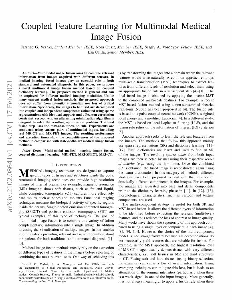
The PCNN-NSST method uses 49 decomposition layers,which is significantly more than the CSR (2 layers) and LLF-IOI (3 layers) methods. Using a larger number of decom-position layers allows PCNN-NSST to capture more relevantinformation, including intensity and texture. Also, the use ofdirectional filters in NSST improves the fusion of featureswith higher structural similarities. However, the PCNN-NSSTmethod occasionally suffers from a non-negligible amountof intensity attenuation, again due to employing a binary-selection rule for resolution-based features (see Figs. 5 and6.). Moreover, the NSST reconstructs the final image solelybased on a sparse representation, which inevitably leads to aloss of texture information. For example, the magnified regionof Fig. 9 shows how the texture of the MR image appears witha significantly lower contrast in the PCNN-NSST result. Notethat the corresponding regions in the SPECT(TI) image areentirely dark, meaning that the texture is expected to appearin the final image unaltered. The proposed method providesgood visual results by preserving both intensity and details.Recall that in the proposed method, the fusion rule is appliedto the correlated features only, which guarantees that binaryselection does not omit any modality-specific information.Moreover, the independent components isolate these modality-specific features and add them directly to the fused imagewithout employing any additional processing that might lead totexture degradation or necessitate expensive computations. Theadvantage of this strategy is evident in functional-anatomicalfusion, where large areas in one of the images can be flator dark in the other image. For example, the regions of theMR image that are dark (no signal) in the PET image ofFig. 9 are well preserved by the proposed method, while allother methods show a loss of the local intensity or decreasedcontrast.
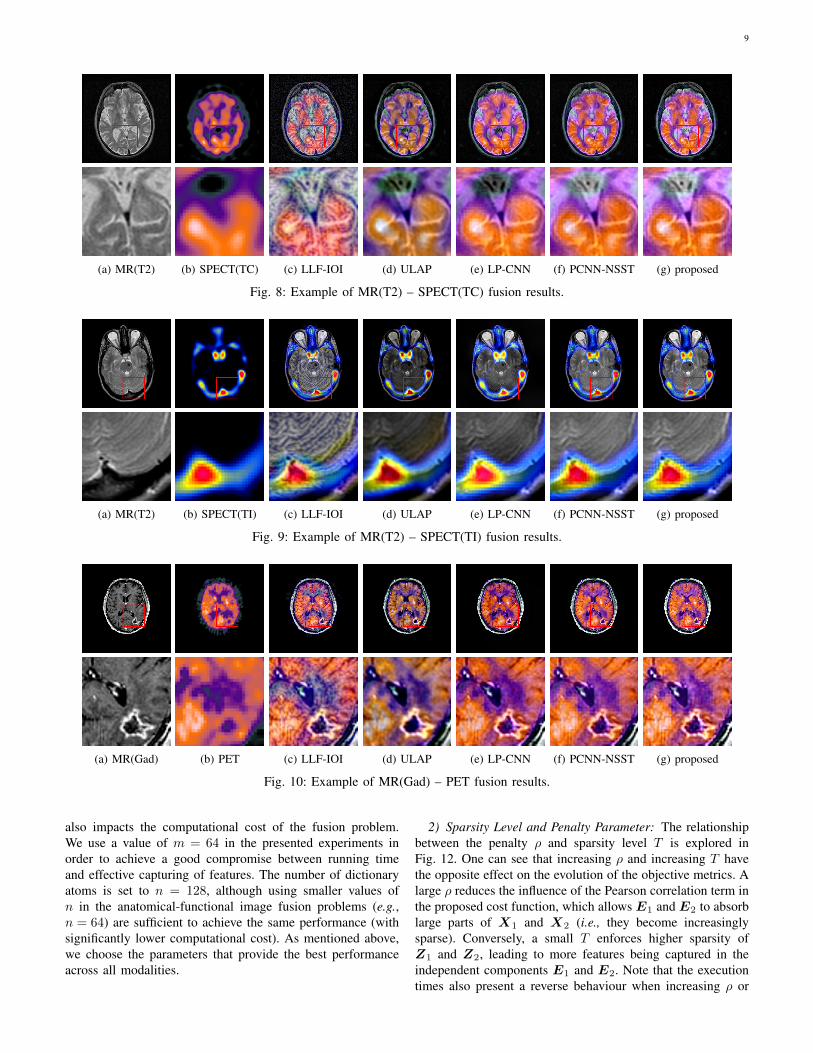
2) Comparison Using Objective Metrics: The results ob-tained based on the objective metrics are reported in Table I.These results are in favour of the proposed method. Specifi-cally, the ULAP and CSR methods provide low STDs, whichis due to the loss of contrast discussed previously. Moreover,the LLF-IOI method always shows relatively low QY andQCB values, which points to the presence of visual artefacts.The objective metrics of the LP-CNN method are almostalways lower than those of the PCNN-NSST and proposedmethods. Finally, the proposed method leads to the best overallperformance (except one experiment where the performance isslightly below that of the ULAP method). These results aresummarized in terms of average objective metrics in Fig. 11,where one can see that the proposed method leads to the bestaverage values over all datasets. These findings show that theproposed method generalizes well to diverse medical imagingmodalities.
3) Execution Times: The average execution times of all theexperiments are reported in Table II. This table shows that theproposed method is competitive with recent multimodal fusionmethods in terms of computational efficiency. Specifically, the

8
(a) CT (b) MR(T2) (c) CSR (d) ULAP (e) LP-CNN (f) PCNN-NSST (g) proposed
Fig. 5: Example of MR(T2) – CT fusion results.
(a) MR(T1) (b) MR(T2) (c) CSR (d) ULAP (e) LP-CNN (f) PCNN-NSST (g) proposed
Fig. 6: Example of MR(T1) – MR(T2) fusion results.
(a) MR(T2) (b) PET (c) LLF-IOI (d) ULAP (e) LP-CNN (f) PCNN-NSST (g) proposed
Fig. 7: Example of MR(T2) – PET fusion results.
running time of the proposed method is comparable to that ofthe PCNN-NSST method and significantly better than those ofthe CSR and LLF-IOI methods. The ULAP method results inthe shortest execution time but does not yield the best results.
C. Effect of Parameters
Because the tested medical imaging modalities are verydifferent, the parameters providing the best performance mayvary between experiments. For example, fusion problemsinvolving one low-detail modality, such as MR-SPECT, are
efficiently tackled by a relatively small sparsity parameterT . In contrast, the MR-CT fusion problem naturally requireshigher values for T to accurately represent the richer detailsin both modalities. However, in this work, the parametersused for the proposed method are not tuned for each pair ofmodalities separately. Instead, we use the parameters providingthe best average performance over all datasets. This choiceallows us also to test the generalisation ability of the parametersetting of the proposed method.
1) Dictionary Parameters: The best patch size is related tothe size of local features in the input images. The patch size
9
(a) MR(T2) (b) SPECT(TC) (c) LLF-IOI (d) ULAP (e) LP-CNN (f) PCNN-NSST (g) proposed
Fig. 8: Example of MR(T2) – SPECT(TC) fusion results.
(a) MR(T2) (b) SPECT(TI) (c) LLF-IOI (d) ULAP (e) LP-CNN (f) PCNN-NSST (g) proposed
Fig. 9: Example of MR(T2) – SPECT(TI) fusion results.
(a) MR(Gad) (b) PET (c) LLF-IOI (d) ULAP (e) LP-CNN (f) PCNN-NSST (g) proposed
Fig. 10: Example of MR(Gad) – PET fusion results.
also impacts the computational cost of the fusion problem.We use a value of m = 64 in the presented experiments inorder to achieve a good compromise between running timeand effective capturing of features. The number of dictionaryatoms is set to n = 128, although using smaller values ofn in the anatomical-functional image fusion problems (e.g.,n = 64) are sufficient to achieve the same performance (withsignificantly lower computational cost). As mentioned above,we choose the parameters that provide the best performanceacross all modalities.
2) Sparsity Level and Penalty Parameter: The relationshipbetween the penalty ρ and sparsity level T is explored inFig. 12. One can see that increasing ρ and increasing T havethe opposite effect on the evolution of the objective metrics. Alarge ρ reduces the influence of the Pearson correlation term inthe proposed cost function, which allows E1 and E2 to absorblarge parts of X1 and X2 (i.e., they become increasinglysparse). Conversely, a small T enforces higher sparsity ofZ1 and Z2, leading to more features being captured in theindependent components E1 and E2. Note that the executiontimes also present a reverse behaviour when increasing ρ or
10
Data-sets Metrics CSR LLF-IOI ULAP LP-CNN PCNN-NSST proposed
MR(T1)-MR(T2)
QY 0.8899 - 0.8359 0.7349 0.8651 0.9336QCB 0.7073 - 0.6769 0.5891 0.7107 0.7351TMQI 0.7745 - 0.7680 0.7694 0.7768 0.7813STD 56.3661 - 66.1464 64.5726 66.2631 68.4629
MR(T2)-CT
QY 0.8007 - 0.7613 0.7573 0.7621 0.8912QCB 0.6112 - 0.5991 0.5659 0.5725 0.6265TMQI 0.7285 - 0.7228 0.7101 0.7277 0.7447STD 65.0380 - 71.4757 84.2350 87.4317 88.3130
MR(T2)-PET
QY 0.6135 0.8462 0.8053 0.8398 0.8257 0.8994QCB 0.6133 0.6630 0.6645 0.6614 0.6327 0.6786TMQI 0.6985 0.7391 0.7298 0.7341 0.7382 0.7438STD 61.9247 75.5607 64.0611 73.2243 78.7324 81.9925
MR(T2)-SPECT(TC)
QY 0.5624 0.7156 0.7480 0.7471 0.8401 0.8512QCB 0.5386 0.6280 0.6130 0.5532 0.6160 0.6339TMQI 0.7023 0.7359 0.7409 0.7357 0.7344 0.7384STD 60.6317 65.2941 57.3897 67.4967 67.8653 70.4694
MR(T2)-SPECT(TI)
QY 0.6610 0.7234 0.7629 0.7765 0.8494 0.8995QCB 0.6252 0.4954 0.5108 0.5029 0.5772 0.5880TMQI 0.6778 0.6956 0.6958 0.6932 0.6941 0.6959STD 52.2014 64.4325 51.1641 67.9101 67.6377 70.0668
MR(Gad)-PET
QY 0.6641 0.7583 0.8340 0.7478 0.8176 0.9105QCB 0.6164 0.6691 0.6876 0.6079 0.6582 0.7204TMQI 0.7232 0.7468 0.7461 0.7396 0.7463 0.7508STD 56.2280 63.3500 55.1129 62.1655 65.0489 67.0991
TABLE I: Objective comparison between different methods. The best performance is shown in bold.
CSR LLF-IOI ULAP LP-CNN PCNN-NSST proposed
Average run-time (s) 34.57 64.58 0.11 12.69 4.62 6.43
TABLE II: Average execution times of different fusion methods.
Fig. 11: Average objective evaluation results using all test datasets for different fusion methods.
T .Fig. 12 also highlights some challenges regarding the pa-
rameter setting. Specifically, the objective metrics QY andQCB evolve in a manner that is inversely proportional toTMQI and STD. More specifically, the former becomeworse when increasing T /lowering ρ, while the latter areimproved. Although decreasing the amount of informationcaptured by the independent components does lead to lossof details; it also increases the amount of energy left in thecorrelated components. Following similar reasoning, loweringT /increasing ρ saturates the independent components and leadsto a loss of contrast. (Note that when the values in the finalfused image exceed 1, they are simply rescaled by clippingthem to the valid intensity range.) This trade-off should betaken into account when setting the parameters of the proposed
method.Based on the observations above, the most suitable param-
eters are T = 5 and ρ = 10 in the presented experiments.
VI. CONCLUSION
A novel image fusion method for multimodal medicalimages. A decomposition method separates input images intotheir correlated and independent components. The correlatedcomponents are captured by sparse representations with identi-cal supports and learnt coupled dictionaries. The independencebetween the independent components is established by mini-mization of pixel-wise Pearson correlations. An alternating op-timization strategy is adopted for addressing the resulting op-timization problem. One particularity of the proposed methodis that it applies a fusion rule to the correlated components

11
Fig. 12: Average objective evaluation results over all test datasets for different values of the penalty parameter ρ and sparsityparameter T . Top: results for different ρ values with T = 5. Bottom: results for different T values with ρ = 10.
only while fully preserving the independent components. Inthe experiments, this strategy has shown superior preservationof intensity and detail compared to other recent methods.Quantitative evaluation metrics and comparison of executiontimes have also shown the competitiveness of the proposedmethod.
REFERENCES
[1] A. P. James and B. V. Dasarathy, “Medical image fusion: A survey ofthe state of the art,” Inf. Fusion, vol. 19, pp. 4–19, 2004.
[2] S. Li, X. Kang, L. Fang, J. Hu, and H. Yin, “Pixel-level image fusion: Asurvey of the state of the art,” Inf. Fusion, vol. 33, pp. 100–112, 2017.
[3] J. Du, W. Li, K. Lu, and B. Xiao, “An overview of multi-modal medicalimage fusion,” Neurocomputing, vol. 215, pp. 3–20, 2004.
[4] M. Yin, X. Liu, Y. Liu, and X. Chen, “Medical image fusion withparameter-adaptive pulse coupled neural network in nonsubsampledshearlet transform domain,” IEEE Trans. Instrum. Meas., vol. 68, no. 1,pp. 49–64, 2019.
[5] J. Du, W. Li, B. Xiao, and Q. Nawaz, “Union Laplacian pyramid withmultiple features for medical image fusion,” Neurocomputing, vol. 194,pp. 326–339, 2016.
[6] G. Bhatnagar, Q. M. J. Wu, and Z. Liu, “Directive contrast basedmultimodal medical image fusion in NSCT domain,” IEEE Trans.Multimedia, vol. 15, no. 5, pp. 1014–1024, 2013.
[7] Y. Liu, S. Liu, and A. Wang, “A general framework for image fusionbased on multi-scale transform and sparse representation,” Inf. Fusion,vol. 24, pp. 1047–1064, 2015.
[8] J. Du, W. Li, , and B. Xiao, “Anatomical-functional image fusion byinformation of interest in local Laplacian filtering domain,” IEEE Trans.Image Process., vol. 26, no. 12, pp. 5855–5865, 2017.
[9] ——, “Fusion of anatomical and functional images using parallelsaliency features,” Inf. Sciences, vol. 430–431, pp. 567–576, 2018.
[10] J. Du, W. Li, , B. Xiao, and Q. Nawaz, “Medical image fusionby combining parallel features on multi-scale local extrema scheme,”Knowledge Based Systems, vol. 113, pp. 4–12, 2016.
[11] Y. Liu, X. Chen, R. K. Ward, and Z. J. Wang, “Image fusion withconvolutional sparse representation,” IEEE Signal Process. Lett., vol. 23,no. 12, pp. 1882–1886, 2016.
[12] ——, “Medical image fusion via convolutional sparsity based morpho-logical component analysis,” IEEE Signal Process. Lett., vol. 26, no. 3,pp. 485–489, 2019.
[13] Y. Jiang and M. Wang, “Image fusion with morphological componentanalysis,” Inf. Fusion, vol. 18, pp. 107–118, 2014.
[14] H. Li, X. He, D. Tao, Y. Tang, and R. Wang, “Joint medical imagefusion, denoising and enhancement via discriminative low-rank sparsedictionaries learning,” Pattern Recognit., vol. 79, pp. 130–146, 2018.
[15] B. Yang and S. Li, “Pixel-level image fusion with simultaneous orthog-onal matching pursuits,” Inf. Fusion, vol. 13, pp. 10–19, 2012.
[16] ——, “Multifocus image fusion and restoration with sparse representa-tion,” IEEE Trans. Instrum. Meas., vol. 59, no. 4, pp. 884–892, 2010.
[17] N. Yu, T. Qiu, F. Bi, and A. Wang, “Image features extraction andfusion based on joint sparse representation,” IEEE J. Sel. Topics SignalProcess., vol. 5, no. 5, pp. 1074–1082, 2011.
[18] J. Yang, Z. Wang, Z. Lin, S. Cohen, and T. Huang, “Coupled dictio-nary training for image super-resolution,” IEEE Trans. Image Process.,vol. 21, no. 8, pp. 3467–3478, 2012.
[19] F. G. Veshki, N. Ouzir, and S. A. Vorobyov, “Image fusion using jointsparse representations and coupled dictionary learning,” in Proc. IEEEInt. Conf. Acoust., Speech Signal Process., Barcelona, Spain, May 2020,pp. 8344–8348.
[20] S. Wang, L. Zhang, Y. Liang, and Q. Pan, “Semi-coupled dictionarylearning with applications to image super-resolution and photo-sketchsynthesis,” in Proc. IEEE Conf. Comput. Vis. Pattern Recognit., Provi-dence, RI, USA, Jun. 2012, pp. 2216–2223.
[21] K. Sharma, S. K. Yadav, B. Valluru, and L. Liu, “Significance of MRIin the diagnosis and differentiation of clear cell sarcoma of tendon andaponeurosis (CCSTA),” Medicine, vol. 97, no. 31, p. e111012, 2018.
[22] M. Aharon, M. Elad, and A. Bruckstein, “K-SVD: an algorithm fordesigning overcomplete dictionaries for sparse representation,” IEEETrans. Signal Process., vol. 54, no. 11, pp. 4311–4322, 2006.
[23] K. Engan, S. O. Aase, and J. H. Husoy, “Method of optimal directions forframe design,” in Proc. IEEE Int. Conf. Acoust., Speech Signal Process.,Phoenix, AZ, USA, Mar. 1999, pp. 2443–2446.
[24] J. Mairal, F. Bach, J. Ponce, and G. Sapiro, “Online dictionary learningfor sparse coding,” in Proc. ACM Int. Conf. Mach. Learn., Montreal,QC, Canada, Jun. 2009, pp. 689–696.
[25] Y. C. Pati, R. Rezaiifar, and P. S. Krishnaprasad, “Orthogonal matchingpursuit: recursive function approximation with applications to waveletdecomposition,” in Conf. Rec. 27th Asilomar Conf. Signals, Syst. Com-put., Pacific Grove, CA, USA, Nov. 1993, pp. 40–44.
[26] J. Tropp, A. Gilbert, and M. Strauss, “Algorithms for simultaneoussparse approximation. part I: greedy pursuit,” Signal Process., vol. 86,p. 572–588, 2006.
[27] F. G. Veshki and S. A. Vorobyov, “An efficient coupled dictionarylearning method,” IEEE Signal Process. Lett., vol. 26, no. 10, pp. 1441–1445, 2019.
[28] J. Sulam and M. Elad, “Expected patch log likelihood with a sparseprior,” in Proc. Int. Workshop Energy Minimization Methods Comput.Vision Pattern Recognit. (EMMCVPR), Hong Kong, China, Jan. 2015,pp. 99–111.
[29] B. Wohlberg, “Efficient algorithms for convolutional sparse representa-tions,” IEEE Trans. Image Process., vol. 25, no. 1, pp. 301–315, 2016.
[30] Y. Liu, X. Chen, J. Cheng, and H. Peng, “A medical image fusion methodbased on convolutional neural networks,” in Proc. 20th Int. Conf. Inf.Fusion, Xi’an, China, Jul. 2017, pp. 1–7.
[31] The Whole Brain Atlas of Harvard Medical School. Accessed: 2020,May. 5. [Online]. Available: http://www.med.harvard.edu/AANLIB/

12
[32] H. Yeganeh and Z. Wang, “Objective quality assessment of tone mappedimages,” IEEE Transactios on Image Processing, vol. 22, no. 2, pp. 657–667, 2013.
[33] C. Yang, J. Q. Zhang, X. R. Wang, and X. Liu, “A novel similarity basedquality metric for image fusion,” Information Fusion, vol. 9, no. 2, pp.156–160, 2008.
[34] Y. Chen and R. S. Blum, “A new automated quality assessment algorithmfor image fusion,” Image and Vision Computing, vol. 27, no. 10, pp.1421–1432, 2009.