i

COUPLED MECHANICAL AND HYDRAULIC MODELING OF

GEOSYNTHETIC-REINFORCED COLUMN-SUPPORTED EMBANKMENTS

By

Jie Huang

B.S., Wuhan University, Wuhan, China, 2000 M.S., Wuhan University, Wuhan, China, 2003

Submitted to the Department of Civil, Environmental, and Architectural Engineering

and the Faculty of the Graduate School of the University of Kansas In partial fulfillment of the requirements for the degree of

Doctor of Philosophy

____________________ Dr. Jie Han, Chairperson

____________________ Committee members Dr. Caroline R. Bennett

____________________ Dr. Weizhang Huang

____________________

Dr. Robert L. Parsons

____________________ Dr. Francis M. Thomas

Date defended: _________

i

The Dissertation Committee for Jie Huang certifies

that this is the approved version of the following dissertation:

COUPLED MECHANICAL AND HYDRAULIC MODELING OF

GEOSYNTHETIC-REINFORCED COLUMN-SUPPORTED EMBANKMENTS

Committee

____________________ Dr. Jie Han, Chairperson

____________________ Dr. Caroline R. Bennett

____________________ Dr. Weizhang Huang

____________________

Dr. Robert L. Parsons

____________________ Dr. Francis M. Thomas

Date approved: _________

ii

ABSTRACT Geosynthetic-reinforced column-supported (GRCS) embankments have been

increasingly used worldwide in the past few years. Even though a number of research

investigations have been completed on this topic, the behavior of GRCS

embankments is not well understood. To improve the understanding of this

technology, coupled mechanical and hydraulic numerical analyses were conducted in

this study under both two-dimensional (2D) and three-dimensional (3D) conditions to

investigate influence of various factors on the performance of GRCS embankments.

The selected parameters and their ranges in this study were based on deep-mixed

(DM) columns; however, a similar study can be conducted for other types of

columns.

2D and 3D models were developed based on elasto-plastic constitutive relationships

with Mohr-Coulomb failure criteria for DM walls or columns, soft soil, firm soil, and

embankment fill. Cable and geogrid elements were selected to simulate geosynthetic

reinforcement in 2D and 3D models, respectively. Staged construction was modeled

by building the embankment in lifts. The ground water table was assumed at the

ground surface. The mechanical model was coupled with the hydraulic model to

simulate the generation and dissipation of excess pore water pressure during and after

the construction.

iii

The 2D and 3D models were calibrated using a well documented case history with

long-term field measurement data and fairly detailed material information to ensure

their reasonableness and adequacy. Upon completion of the model calibrations, a 2D

baseline case based on a typical configuration of GRCS embankment was analyzed.

A 2D parametric study was conducted by changing the parameters individually from

the baseline case to investigate the influence of that factor on the performance of the

embankment including post-construction settlement, post-construction differential

settlement, distortion, tension in geosynthetic, effective stress, stress concentration

ratio, excess pore water pressure, and degree of consolidation. The investigated

factors include soft soil modulus, soft soil friction angle, soft soil permeability, DM

column modulus, DM column spacing, geosynthetic tensile stiffness, and average

construction rate.

After the 2D study was completed, the 2D baseline case was converted into a 3D

baseline case based on an area-weighted average approach assuming a square pattern

of DM columns. The 3D parametric study was preformed by changing parameters

individually from the 3D baseline case to investigate the influence of that specific

factor on the performance of the embankment. The factors investigated are the same

as those in the 2D parametric study.

iv

On the basis of the numerical results from the 2D and 3D studies, the influence of

factors on the performance of the embankment system was rated to provide guidance

for practical use.

v

ACKNOWLEDGEMENTS I would like to express my sincere gratitude and appreciation to Dr. Jie Han, my

advisor and committee chair, for his guidance, encourage, inspiration, and support

during the course of my doctoral study. It has been an unforgettable experience to

work under his supervision.

My thanks also go to my committee members, Profs. Caroline R. Bennett, Weizhang

Huang, Robert L. Parsons, and Francis M. Thomas, for their valuable input and

suggestions.

I would like to thank my wife, Juan Mao, for her sacrifice and support. Juan took care

of me and encouraged me in the vital periods of my doctoral study. In addition, she

has brought great joy to my life.

Special thank is given to Dr. Sadik Oztoprak at Istanbul University, Turkey for

sharing his research experience on embankments over soft soil and giving insightful

suggestions during his visit at the University of Kansas.

Finally, I would like to thank my fellow classmates: Sheryl Gallagher, Rebecca

Johnson, Elizabeth Kneebone, Matthew Pierson, Harihar Shiwakoti, Xiaoming Yang,

vi

and Yuze Zhang, for their help. It has been a great pleasure to discuss and even argue

with them.

vii

TABLE OF CONTENTS

ABSTRACT ii

ACKNOWLEDGEMENT v

TABLE OF CONTENTS vii

LIST FIGURES xii

LIST OF TABLES xxiv

CHAPTER ONE INTRODUCTION 1

1.1 Background 1

1.2 Column Supported (CS) and Geosynthetic-Reinforced Column-Supported (GRCS)

Embankments 3

1.2.1 History of CS and GRCS Embankments 5

1.2.2 Brief Characterization and Comparison of CS and GRCS Embankments 7

1.3 Purpose and Scope of This Study 11

1.4 Organization of This Dissertation 12

CHAPTER TWO LITERATURE REVIEW 15

2.1 Introduction 15

viii

2.2 Load Transfer Mechanisms of GRCS Embankments 15

2.2.1 Soil Arching Theories 17

2.2.2 Tensioned Membrane Theories 32

2.3 Current Design Methodologies for GRCS Embankments 39

2.4 Current Research Status 47

CHAPTER THREE MODEL CALIBRATIONS 52

3.1 Introduction 52

3.2 Selected Case Study 54

3.3 Numerical Modeling 60

3.4 Two-dimensional (2D) Model Calibration 62

3.4.1 Numerical Modeling 62

3.4.2 Results and Comparison 67

3.5 Three-dimensional (3D) Model Calibration 76

3.5.1 Numerical Modeling 77

3.5.2 Results and Comparison 80

CHAPTER FOUR TWO-DIMENSIONAL PARAMETRIC STUDY 86

4.1 2D Baseline Case 86

ix

4.1.1 2D Dimensions and Properties 86

4.1.2 2D Modeling Procedure 89

4.1.3 Results of 2D Baseline Case 92

4.2 2D Parametric Study 113

4.2.1 Outline of 2D Parametric Study 113

4.2.2 Settlement 115

4.2.3 Tension Developed in Geosynthetics 150

4.2.4 Vertical Stress and Stress Concentration Ratio 166

4.2.5 Excess Pore Water Pressure 187

CHAPTER FIVE THREE-DIMENSIONAL PARAMETRIC STUDY 199

5.1 3D Baseline Case 200

5.1.1 3D Dimensions and Properties 200

5.1.2 3D Modeling Procedure 204

5.1.3 3D Results of Baseline Case 204

5.2 3D Parametric Study 223

x

5.2.1 Outline of 3D Parametric Study 223

5.2.2 Settlement 224

5.2.3 Tension Developed in Geosynthetics 274

5.2.4 Vertical Stress and Stress Concentration Ratio 281

5.2.5 Excess Pore Water Pressure 310

CHAPTER SIX COMPARISON OF TWO-DIMENSIONAL AND THREE

DIMENSIONAL STUDIES 323

6.1 Verification of Simplified Model 324

6.2 2D and 3D Comparisons 329

6.2.1 Maximum Settlement and Distortion 330

6.2.2 Maximum Tension Developed in Geosynthetics 342

6.2.3 Maximum Stress Concentration ratio 349

6.2.4 Excess Pore Water Pressure 356

6.2.5 Summary 363

CHAPTER SEVEN CONCLUSIONS AND RECOMMENDATIONS 367

7.1 Conclusions 367

7.2 Recommendations 374

xi

7.3 Future Work 375

REFERENCES 377

xii

LIST OF FIGURES Fig. 1-1. Cross-sections of CS and GRCS Embankments 6

Fig. 1-2. Geosynthetic Preventing Slope Lateral Spreading 10

Fig. 2-1. Soil Arching and Tensioned Membrane Effects in GRCS Embankments 17

Fig. 2-2. Terzaghi’s Soil Arching Model 21

Fig. 2-3. Soil Arching above Continuous Supports 24

Fig. 2-4. Soil Arches above Column Grid of Square Pattern 26

Fig. 2-5. Finn’s Pure Translation and Pure Rotation Models 29

Fig. 2-6. Delmas’ and Giroud’s Membrane Models 33

Fig. 2-7. Load Carrying Area of Geosynthetics 36

Fig. 2-8. Soil Arching Ratio 45

Fig. 2-9. Tension in Geosynthetic Reinforcement 46

Fig. 3-1. Profile of Sipoo River Bridge Embankment 55

Fig. 3-2. Embankment Cross-section and Column Layout 58

Fig. 3-3. Arrangement of Instrumentations 59

Fig. 3-4. Construction Process 61

Fig. 3-5. Modeling Procedure 61

Fig. 3-6. 2D Numerical Model 64

Fig. 3-7. FLAC Models 66

Fig. 3-8. Settlement Profiles at Different Stages (2D) 68

Fig. 3-9. Settlement versus Time (2D) 69

Fig. 3-10. Settlement Profiles at the Base and on the Crest of the Embankment (2D) 72

Fig. 3-11. Strain versus Time (2D) 74

Fig. 3-12. Tension Developed in the Geosynthetic Layer with or without Mid-DM Walls 75

Fig. 3-13. 3D Numerical Model 78

xiii

Fig. 3-14. FLAC3D Model 79

Fig. 3-15. Settlement Profiles at Different Stages (3D) 80

Fig. 3-16. Settlement versus Time (3D) 82

Fig. 3-17. Settlement Profiles on the Crest and at the Base (3D) 83

Fig. 3-18. Strain versus Time (3D) 85

Fig. 4-1. Two-dimensional Model of the Baseline Case 87

Fig. 4-2. Modeling of Staged Construction 91

Fig. 4-3. Settlement Contour of the 2D Baseline Case 92

Fig. 4-4. Settlement versus Time of the 2D Baseline Case 93

Fig. 4-5. Settlement Profiles of the 2D Baseline Case at Different Time 96

Fig. 4-6. Differential Settlement 97

Fig. 4-7. Tension Distribution of the 2D Baseline Case 98

Fig. 4-8. Tension Profiles of the 2D Baseline Case 99

Fig. 4-9. Post-construction Tension Profiles of the 2D Baseline Case 100

Fig. 4-10. Tension Profiles of the 2D Baseline Case at 30 Years after Service 100

Fig. 4-11. Tension versus Time of the 2D Baseline Case 101

Fig. 4-12. Vertical Effective Stress Contour of the 2D Baseline Case 102

Fig. 4-13. Vertical Stress Distribution of the 2D Baseline Case 103

Fig. 4-14. Additional Vertical Effective Stress versus Time of the 2D Baseline Case 105

Fig. 4-15. Stress Concentration Ratio Calculation Illustration 106

Fig. 4-16. Stress Concentration Ratio Profiles of the 2D Baseline Case 107

Fig. 4-17. Pore Water Pressure Contour of the 2D Baseline Case 108

Fig. 4-18. Excess Pore Water Pressure at Point C and D versus Time of the 2D Baseline Case 109

Fig. 4-19. Excess Pore Water Pressure at Point D and E versus Time of the 2D Baseline Case 110

Fig. 4-20. Excess Pore Water Pressure versus Depth of the 2D Baseline Case 111

Fig. 4-21. Excess Pore Water Pressure or Additional Vertical Effective Stress versus Time of the 2D Baseline Case 112

xiv

Fig. 4-22. Settlement Profiles for Various Soil Moduli at 1 Month after Service (2D) 117

Fig. 4-23. Settlement Profiles for Various Soil Moduli at 30 Years after Service (2D) 118

Fig. 4-24. Maximum Settlement versus Soil Modulus (2D) 119

Fig. 4-25. Maximum Differential Settlement versus Soil Modulus (2D) 119

Fig. 4-26. Maximum Distortion on the Crest versus Soil Modulus (2D) 120

Fig. 4-27. Settlement Profiles for Various Friction Angles at 1 Month after Service (2D) 122

Fig. 4-28. Settlement Profiles for Various Friction Angles at 30 Years after Service (2D) 123

Fig. 4-29. Maximum Settlement versus Friction Angle (2D) 124

Fig. 4-30. Maximum Differential Settlement versus Friction Angle (2D) 124

Fig. 4-31. Maximum Distortion on the Crest versus Friction Angle (2D) 125

Fig. 4-32. Settlement Profiles for Various Permeability at 1 Month after Service (2D) 126

Fig. 4-33. Settlement Profiles for Various Permeability at 30 Years after Service (2D) 127

Fig. 4-34. Maximum Settlement versus Soil Permeability (2D) 128

Fig. 4-35. Maximum Differential Settlement versus Soil Permeability (2D) 129

Fig. 4-36. Maximum Distortion on the Crest versus Soil Permeability (2D) 130

Fig. 4-37. Settlement Profiles for Various Column Moduli at 1 Month after Service (2D) 132

Fig. 4-38. Settlement Profiles for Various Column Moduli at 30 Years after Service (2D) 133

Fig. 4-39. Maximum Settlement versus Column Modulus (2D) 134

Fig. 4-40. Maximum Differential Settlement versus Column Modulus (2D) 134

Fig. 4-41. Maximum Distortion on the Crest versus Column Modulus (2D) 136

Fig. 4-42. Settlement Profiles for Various Column Spacing at 1 Month after Service (2D) 137

Fig. 4-43. Settlement Profiles for Various Column Spacing at 30 Years after Service (2D) 138

Fig. 4-44. Maximum Settlement versus Column Spacing (2D) 139

Fig. 4-45. Maximum Differential Settlement versus Column Spacing (2D) 140

xv

Fig. 4-46. Maximum Distortion on the Crest versus Column Spacing (2D) 140

Fig. 4-47. Settlement Profiles for Various Tensile Stiffness at 1 Month after Service (2D) 142

Fig. 4-48. Settlement Profiles for Various Tensile Stiffness at 30 Years after Service (2D) 143

Fig. 4-49. Maximum Settlement versus Tensile Stiffness (2D) 144

Fig. 4-50. Maximum Differential Settlement versus Tensile Stiffness (2D) 144

Fig. 4-51. Maximum Distortion on the Crest versus Tensile Stiffness (2D) 145

Fig. 4-52. Settlement Profiles for Various Average Construction Rates at 1 Month after Service (2D) 147

Fig. 4-53. Settlement Profiles for Various Average Construction Rates at 30 Years after Service (2D) 148

Fig. 4-54. Maximum Settlement versus Average Construction Rate (2D) 149

Fig. 4-55. Maximum Differential Settlement versus Average Construction Rate (2D) 149

Fig. 4-56. Maximum Distortion on the Crest versus Average Construction Rate (2D) 150

Fig. 4-57. Tension Profiles for Various Soil Moduli at 1 Month and 30 Years after Service (2D) 152

Fig. 4-58. Maximum Tension versus Soil Modulus (2D) 153

Fig. 4-59. Tension Profiles for Various Friction Angles at 1 Month and 30 Years after Service (2D) 154

Fig. 4-60. Maximum Tension versus Friction Angle (2D) 155

Fig. 4-61. Tension Profiles for Various Soil Permeability at 1 Month and 30 Years after Service (2D) 156

Fig. 4-62. Maximum Tension versus Soil Permeability (2D) 157

Fig. 4-63. Tension Profiles for Various Column Moduli at 1 Month and 30 Years after Service (2D) 158

Fig. 4-64. Maximum Tension versus Column Modulus (2D) 159

Fig. 4-65. Tension Profiles for Various Column Spacing at 1 Month and 30 Years after Service (2D) 160

Fig. 4-66. Maximum Tension versus Column Spacing (2D) 161

Fig. 4-67. Tension Profiles for Various Tensile Stiffness at 1 Month and 30 Years after Service (2D) 162

xvi

Fig. 4-68. Maximum Tension versus Tensile Stiffness (2D) 163

Fig. 4-69. Tension Profiles for Various Average Construction Rates at 1 Month and 30 Years after Service (2D) 164

Fig. 4-70. Maximum Tension versus Average Construction Rate (2D) 165

Fig. 4-71. Additional Vertical Effective Stress Profiles for Various Soil Moduli (2D) 167

Fig. 4-72. Stress Concentration Ratio Profiles for Various Soil Moduli (2D) 169

Fig. 4-73. Additional Effective Stress Profiles for Various Friction Angles (2D) 170

Fig. 4-74. Stress Concentration Ratio Profiles for Various Friction Angles (2D) 172

Fig. 4-75. Additional Effective Stress Profiles for Various Soil Permeability (2D) 174

Fig. 4-76. Stress Concentration Ratio Profiles for Various Soil Permeability (2D) 175

Fig. 4-77. Additional Vertical Effective Stress Profiles for Various Column Moduli (2D) 176

Fig. 4-78. Stress Concentration Ratio Profiles for Various Column Moduli (2D) 177

Fig. 4-79. Additional Vertical Effective Stress Profiles for Various Column Spacing (2D) 179

Fig. 4-80. Stress Concentration Ratio Profiles for Various Column Spacing (2D) 180

Fig. 4-81. Additional Vertical Effective Stress Profiles for Various Tensile Stiffness (2D) 181

Fig. 4-82. Stress concentration Ratio Profiles for Various Tensile Stiffness (2D) 183

Fig. 4-83. Additional Vertical Effective Stress Profiles for Various Average Construction Rates (2D) 184

Fig. 4-84. Stress Concentration Ratio Profiles for Various Average Construction Rates (2D) 186

Fig. 4-85. Excess Pore Water Pressure Distributions for Various Soil Moduli (2D) 189

Fig. 4-86. Degree of Consolidation versus Soil Modulus (2D) 189

Fig. 4-87. Excess Pore Water Pressure Distributions for Various Friction Angles (2D) 190

Fig. 4-88. Degree of Consolidation versus Friction Angle (2D) 191

Fig. 4-89. Excess Pore Water Pressure Distributions for Various Soil Permeability (2D) 192

Fig. 4-90. Degree of Consolidation versus Soil Permeability (2D) 192

Fig. 4-91. Excess Pore Water Pressure Distributions for Various Column Moduli (2D) 193

xvii

Fig. 4-92. Degree of Consolidation versus Column Modulus (2D) 194

Fig. 4-93. Excess Pore Water Pressure Distributions for Various Column Spacing (2D) 195

Fig. 4-94. Degree of Consolidation versus Column Spacing (2D) 195

Fig. 4-95. Excess Pore Water Pressure Distributions for Various Tensile Stiffness (2D) 196

Fig. 4-96. Degree of Consolidation versus Tensile Stiffness (2D) 197

Fig. 4-97. Excess Pore Water Pressure Distributions for Various Average Construction Rates (2D) 198

Fig. 4-98. Degree of Consolidation versus Average Construction Rate (2D) 198

Fig. 5-1. Three-dimensional Model of the 3D Baseline Case 201

Fig. 5-2. Conversion of Column Modulus 203

Fig. 5-3. Settlement Contour of the 3D Baseline Case 205

Fig. 5-4. Settlement versus Time of the 3D Baseline Case 206

Fig. 5-5. Settlement Profiles of the 3D Baseline Case at Different Time 208

Fig. 5-6. Tension Contours of the 3D Baseline Case 210

Fig. 5-7. Tension Profiles of the 3D Baseline Case 212

Fig. 5-8. Tension versus Time of the 3D Baseline Case 213

Fig. 5-9. Vertical Effective Stress Contour of the 3D Baseline Case 214

Fig. 5-10. Effective Stress Distribution of the 3D Baseline Case 214

Fig. 5-11. Additional Vertical Effective Stress versus Time of the 3D Baseline Case 215

Fig. 5-12. Stress Concentration Ratio Profiles of the 3D Baseline Case 217

Fig. 5-13. Pore Water Pressure Contour of the 3D Baseline Case 218

Fig. 5-14. Excess Pore Water Pressure at Point C1 and D1 versus Time of the 3D Baseline Case 218

Fig. 5-15. Excess Pore Water Pressure at Point D1 and E1 versus Time of the 3D Baseline Case 219

Fig. 5-16. Excess Pore Water Pressure versus Depth of the 3D Baseline Case 221

Fig. 5-17. Excess Pore water Pressure or Additional Vertical Effective Stress versus Time of the 3D Baseline Case 222

xviii

Fig. 5-18. Settlement Profiles for Various Soil Moduli at 1 Month after Service (3D) 225

Fig. 5-19. Settlement Profiles for Various Soil Moduli at 4.5 Years after Service (3D) 227

Fig. 5-20. Maximum Settlement versus Soil Modulus (3D) 230

Fig. 5-21. Maximum Differential Settlement versus Soil Modulus (3D) 230

Fig. 5-22. Maximum Distortion on the Crest versus Soil Modulus (3D) 231

Fig. 5-23. Settlement Profiles for Various Friction Angles at 1 Month after Service (3D) 232

Fig. 5-24. Settlement Profiles for Various Friction Angles at 4.5 Years after Service (3D) 234

Fig. 5-25. Maximum Settlement versus Friction Angle (3D) 237

Fig. 5-26. Maximum Differential Settlement versus Friction Angle (3D) 237

Fig. 5-27. Maximum Distortion on the Crest versus Friction Angle (3D) 238

Fig. 5-28. Settlement Profiles for Various Soil Permeability at 1 Month after Service (3D) 240

Fig. 5-29. Settlement Profiles for Various Soil Permeability at 4.5 Years after Service (3D) 242

Fig. 5-30. Maximum Settlement versus Soil Permeability (3D) 244

Fig. 5-31. Maximum Differential Settlement versus Soil Permeability (3D) 245

Fig. 5-32. Maximum Distortion on the Crest versus Soil Permeability (3D) 245

Fig. 5-33. Settlement Profiles for Various Column Moduli on at 1 Month after Service (3D) 247

Fig. 5-34. Settlement Profiles for Various Column Moduli at 4.5 Years after Service (3D) 249

Fig. 5-35. Maximum Settlement versus Column Modulus (3D) 251

Fig. 5-36. Maximum Differential Settlement versus Column Modulus (3D) 252

Fig. 5-37. Maximum Distortion on the Crest versus Column Modulus (3D) 252

Fig. 5-38. Settlement Profiles for Various Column Spacing on at 1 Month after Service (3D) 254

Fig. 5-39. Settlement Profiles for Various Column Spacing on at 4.5 Years after Service (3D) 256

Fig. 5-40. Maximum Settlement versus Column Spacing (3D) 258

Fig. 5-41. Maximum Differential Settlement versus Column Spacing (3D) 259

xix

Fig. 5-42. Maximum Distortion on the Crest versus Column Spacing (3D) 259

Fig. 5-43. Settlement Profiles for Various Tensile Stiffness at 1 Month after Service (3D) 261

Fig. 5-44. Settlement Profiles for Various Tensile Stiffness at 4.5 Years after Service (3D) 263

Fig. 5-45. Maximum Settlement versus Tensile Stiffness (3D) 265

Fig. 5-46. Maximum Differential Settlement versus Tensile Stiffness (3D) 266

Fig. 5-47. Maximum Distortion on the Crest versus Tensile Stiffness (3D) 266

Fig. 5-48. Settlement Profiles for Various Average Construction Rates at 1 Month after Service (3D) 268

Fig. 5-49. Settlement Profiles for Various Average Construction Rates at 4.5 Years after Service (3D) 270

Fig. 5-50. Maximum Settlement versus Average Construction Rate (3D) 272

Fig. 5-51. Maximum Differential Settlement versus Average Construction Rate (3D) 273

Fig. 5-52. Maximum Distortion on the Crest versus Average Construction Rate (3D) 273

Fig. 5-53. Maximum Tension versus Soil Modulus (3D) 275

Fig. 5-54. Maximum Tension versus Friction Angle (3D) 276

Fig. 5-55. Maximum Tension versus Soil Permeability (3D) 277

Fig. 5-56. Maximum Tension versus Column Modulus (3D) 278

Fig. 5-57. Maximum Tension versus Column Spacing (3D) 279

Fig. 5-58. Maximum Tension versus Tensile Stiffness (3D) 280

Fig. 5-59. Maximum Tension versus Average Construction Rate (3D) 281

Fig. 5-60. Additional Vertical Effective Stress Profiles for Various Soil Moduli at 1 Month after Service (3D) 282

Fig. 5-61. Additional Vertical Effective Stress Profiles for Various Soil Moduli at 4.5 Years after Service (3D) 283

Fig. 5-62. Stress Concentration Ratio Profiles for Various Soil Moduli (3D) 285

Fig. 5-63. Additional Vertical Effective Stress Profiles of Various Friction Angles at 1 Month after Service (3D) 286

Fig. 5-64. Additional Vertical Effective Stress Profiles for Various Friction Angles at 4.5 Years after Service (3D) 287

xx

Fig. 5-65. Stress Concentration Ratio Profiles for Various Soil Friction Angles (3D) 289

Fig. 5-66. Additional Effective Stress Profiles for Various Soil Permeability at 1 Month after Service (3D) 290

Fig. 5-67. Additional Effective Stress Profiles for Various Soil Permeability at 4.5 Years after Service (3D) 291

Fig. 5-68. Stress Concentration Ratio Profiles for Various Soil Permeability (3D) 293

Fig. 5-69. Additional Vertical Effective Stress Profiles for Various Column Moduli at 1 Month after Service (3D) 294

Fig. 5-70. Additional Vertical Effective Stress Profiles for Various Column Moduli at 4.5 Years after Service (3D) 295

Fig. 5-71. Stress Concentration Ratio Profiles for Various Column Moduli (3D) 297

Fig. 5-72. Additional Vertical Effective Stress Profiles of Various Column Spacing at 1 Month after Service (3D) 298

Fig. 5-73. Additional Vertical Effective Stress Profiles of Various Column Spacing at 4.5 Years after Service (3D) 299

Fig. 5-74. Stress Concentration Ratio Profiles for Various Column Spacing (3D) 301

Fig. 5-75. Additional Vertical Effective Stress Profiles for Various Tensile Stiffness at 1 Month after Service (3D) 302

Fig. 5-76. Additional Vertical Effective Stress Profiles for Various Tensile Stiffness at 4.5 Years after Service (3D) 303

Fig. 5-77. Stress Concentration Ratio Profiles for Various Tensile Stiffness (3D) 305

Fig. 5-78. Additional Vertical Effective Stress Profiles for Various Average Construction Rates at 1 Month after Service (3D) 306

Fig. 5-79. Additional Vertical Effective Stress Profiles for Various Average Construction Rates at 4.5 Years after Service (3D) 307

Fig. 5-80. Stress Concentration Ratio Profiles for Various Average Construction Rates (3D) 309

Fig. 5-81. Excess Pore Water Pressure Distributions for Various Soil Moduli (3D) 311

Fig. 5-82. Degree of Consolidation versus Soil Modulus (3D) 312

Fig. 5-83. Excess Pore Water Pressure Distributions for Various Friction Angles (3D) 313

Fig. 5-84. Degree of Consolidation versus Friction Angle (3D) 313

Fig. 5-85. Excess Pore Water Pressure Distributions for Various Soil Permeability (3D) 314

xxi

Fig. 5-86. Degree of Consolidation versus Soil Permeability (3D) 315

Fig. 5-87. Excess Pore Water Pressure Distributions for Various Column Moduli (3D) 317

Fig. 5-88. Degree of Consolidation versus Various Column Moduli (3D) 317

Fig. 5-89. Excess Pore Water Pressure Distributions for Various Column Spacing (3D) 318

Fig. 5-90. Degree of Consolidation versus Column Spacing (3D) 319

Fig. 5-91. Excess Pore Water Pressure Distributions for Various Tensile Stiffness (3D) 320

Fig. 5-92. Degree of Consolidation versus Tensile Stiffness (3D) 320

Fig. 5-93. Excess Pore Water Pressure Distributions for Various Average Construction Rates (3D) 321

Fig. 5-94. Degree of Consolidation versus Average Construction Rate (3D) 322

Fig. 6-1. Comparison of Maximum Settlement 325

Fig. 6-2. Comparison of Maximum Distortion 326

Fig. 6-3. Comparison of Maximum Tension 327

Fig. 6-4. Comparison of Maximum Stress Concentration Ratio 328

Fig. 6-5. Comparison of Degree of Consolidation 329

Fig. 6-6. Maximum Settlement versus Soil Modulus under 2D and 3D Conditions 331

Fig. 6-7. Maximum Distortion versus Soil Modulus under 2D and 3D Conditions 332

Fig. 6-8. Maximum Settlement versus Friction Angle under 2D and 3D Conditions 333

Fig. 6-9. Maximum Distortion versus Friction Angle under 2D and 3D Conditions 334

Fig. 6-10. Maximum Settlement versus Soil Permeability under 2D and 3D Conditions 335

Fig. 6-11. Maximum Distortion versus Soil Permeability under 2D and 3D Conditions 335

Fig. 6-12. Maximum Settlement versus Column Modulus under 2D and 3D Conditions 336

Fig. 6-13. Maximum Distortion versus Column Modulus under 2D and 3D Conditions 337

Fig. 6-14. Maximum Settlement versus Column Spacing under 2D and 3D Conditions 338

xxii

Fig. 6-15. Maximum Distortion versus Column Spacing under 2D and 3D Conditions 338

Fig. 6-16. Maximum Settlement versus Tensile Stiffness under 2D and 3D Conditions 340

Fig. 6-17. Maximum Distortion versus Tensile Stiffness under 2D and 3D Conditions 340

Fig. 6-18. Maximum Settlement versus Average Construction Rate under 2D and 3D Conditions 341

Fig. 6-19. Maximum Distortion versus Average Construction Rate under 2D and 3D Conditions 342

Fig. 6-20. Maximum Tension versus Soil Modulus under 2D and 3D Conditions 343

Fig. 6-21. Maximum Tension versus Friction Angle under 2D and 3D Conditions 344

Fig. 6-22. Maximum Tension versus Soil Permeability under 2D and 3D Conditions 345

Fig. 6-23. Maximum Tension versus Column Modulus under 2D and 3D Conditions 346

Fig. 6-24. Maximum Tension versus Column Spacing under 2D and 3D Conditions 347

Fig. 6-25. Maximum Tension versus Tensile Stiffness under 2D and 3D Conditions 348

Fig. 6-26. Maximum Tension versus Average Construction Rate under 2D and 3D Conditions 349

Fig. 6-27. Maximum Stress Concentration Ratio versus Soil Modulus under 2D and 3D Conditions 350

Fig. 6-28. Maximum Stress Concentration Ratio versus Friction Angle under 2D and 3D Conditions 351

Fig. 6-29. Maximum Stress Concentration Ratio versus Soil Permeability under 2D and 3D Conditions 352

Fig. 6-30. Maximum Stress Concentration Ratio versus Column Modulus under 2D and 3D Conditions 353

Fig. 6-31. Maximum Stress Concentration Ratio versus Column Spacing under 2D and 3D Conditions 354

Fig. 6-32. Maximum Stress Concentration Ratio versus Tensile Stiffness under 2D and 3D Conditions 355

Fig. 6-33. Maximum Stress Concentration Ratio versus Average Construction Rate under 2D and 3D Conditions 356

xxiii

Fig. 6-34. Degree of Consolidation versus Soil Modulus under 2D and 3D Conditions 357

Fig. 6-35. Degree of Consolidation versus Friction Angle under 2D and 3D Conditions 358

Fig. 6-36. Degree of Consolidation versus Soil Permeability under 2D and 3D Conditions 359

Fig. 6-37. Degree of Consolidation versus Column Modulus under 2D and 3D Conditions 360

Fig. 6-38. Degree of Consolidation versus Column Spacing under 2D and 3D Conditions 361

Fig. 6-39. Degree of Consolidation versus Tensile Stiffness under 2D and 3D Conditions 362

Fig. 6-40. Degree of Consolidation versus Average Construction Rate under 2D and 3D Conditions 363

xxiv

LIST OF TABLES Table 1-1. Main Advantages and Disadvantages of Embankment Settlement Control

Techniques 2

Table 1-2. Possible Column Types 4

Table 1-3. Constructed GRCS Embankments 8

Table 1-4. Guideline for the Design of Necessary Coverage by Pile Caps 9

Table 2-1. Information of Embankment A and B Used in Comparison 44

Table 2-2. Finished Study on GRCS Embankments 47

Table 3-1. Soil Index Properties 56

Table 3-2. Properties of Soft Clay 56

Table 3-3. Construction Information 59

Table 3-4. Material Properties 65

Table 3-5. Maximum Settlements at the Base of the Embankment 71

Table 3-6. Maximum Tension in the Geosynthetic Layer 76

Table 4-1. Properties of Materials in the 2D Baseline Case 88

Table 4-2. Modeling Procedure 90

Table 4-3. Maximum Differential Settlement and Maximum Distortion of the 2D Baseline case 98

Table 4-4. Parameters and Variation Used in the 2D Study 113

Table 5-1. Properties of Materials in the 3D Baseline Case 203

Table 5-2. Maximum Differential Settlement and Maximum Distortion of the 3D Baseline Case 209

Table 5-3. Parameters and Variation Used in the 3D Study 223

Table 6-1. The Degree of Influence under a 3D Condition 365

xxv

Table 6-2. The Degree of Influence under a 2D Condition 365

Table 6-3. The Influence of Factors under a 3D Condition 366

Table 6-4. The Influence of Factors under a 2D Condition 366

1

CHAPTER ONE

INTRODUCTION

1.1 Background

As the development of modern society progresses, transportation demand grows

dramatically year by year. Numerous embankments have been built to support

roadways and railways. Inevitably, soft clays (for example, alluvial soil and peat) and

other highly compressible soft soils, which used to be considered technically

unsuitable for construction, are encountered. Their adverse features, such as low shear

strength, high compressibility and so on, challenge the geotechnical profession (Bell

et al. 1994; Han 1999). They set constraints on design and construction of earth

structures, such as the maximum dimension of embankments and the maximum

construction rate. To break through these constraints, geotechnical engineers never

stop seeking better means technically and economically. In the past several decades,

many innovative means have been practiced to control post-construction settlements

of embankments built over problematic soils (Hewllet and Randolph 1988; Jones et

al. 1994; Magnan 1994). The main techniques used to control embankment

settlements are listed and compared in Table 1-1.

2

Table 1-1. Main Advantages and Disadvantages of Embankment Settlement Control Techniques (Modified from Magnan 1994)

Technique Advantage Disadvantage

Preloading

It is almost the easiest method among those

techniques. It does not require extra materials except for preloading

weight. It is very efficient, if enough consolidation time

is allowed.

Waiting time for consolidation might be very long and hard to estimate, so monitoring might be needed to determine the degree of consolidation. Sometimes, the transportation and disposal of the preloading weights could increase the total cost.

Preloading with vertical drain

Easy to practice and much faster than preloading.

The cost increases, as either sand well or fabricated vertical drain is involved. Compared with sand well, the installation of fabricated vertical drain is much easier and much faster than the construction of sand well. Since the discharge capacity of fabricated vertical drain is hard to estimate precisely, monitoring may be needed to determine the degree of consolidation.

Vacuum preloading

Compared with the two preceding preloading

techniques, it saves time and cost on transporting preloading weights.

Theoretically speaking, the maximum load that could be applied is atmospheric pressure. And efficient pumping equipment and impervious membrane are vital. Limited experiences are available.

Overexcavation/ Replacement

A fast and easy to use method.

The disposal of extracted soil and transportation of the new fill material increase the cost. It is an expensive method for a large area and/or deep excavation. Therefore, it is hardly used on embankments covering large area. In addition, some other issues have to taken into consideration, such as stability of the cut edge, dewatering if ground water is to be encountered.

Pile Fast and effective Expensive

Piled raft Fast, effective, and reliable It is almost the most expensive technique among those discussed. It is typically used for bridge approach embankment.

Stone column, sand column, and

rammed aggregate pier

Fast

They are expensive. And hazardous vibration could be generated during the construction. Besides, they could not be used in very soft soil situation, since stones and sand need some confinement to sustain their strength. The advent of encased stone columns and sand columns seems to help break through this limitation. But the construction method of encased stone columns and sand columns has not well developed.

Lightweight material

Fast and easy to handle. It has the least disturbance on

in-situ soils.

The lightweight material with reasonable strength is expensive. Typically, protective cover is needed.

3

Table 1-1. Main Advantages and Disadvantages of Embankment Settlement Control Techniques (continued, Modified from Magnan 1994)

Technique Advantage Disadvantage

Jet-grouting Fast and reliable method. It is a very popular

ground improvement technique. A lot of experience could be referred to.

Expensive.

Electro-osmosis Very expensive but not reliable. Destruction of electrodes, electricity needed.

Geosynthetic reinforcement

Installation is very easy. Besides as reinforcement, it could also serve as

separation between embankment fill and foundation soil to avoid the penetration of

granular materials into soft soil.

It is not an effective method if does not combine with other stiffer inclusions such as piles, stone columns.

Geosynthetic-reinforced column-supported system

Compared with using geosynthetic reinforcement alone, it is more effective. And

compared with using piles alone, it is more economical.

Both experiences are limited and theories have not been well-established.

Among the techniques listed in Table 1-1, the geosynthetic-reinforced column-

supported (GRCS) embankment is the focus of this study. Since GRCS originated

from column supported (CS) embankments, both CS embankments and GRCS

embankments will be briefly reviewed in this chapter.

1.2 Column Supported (CS) and Geosynthetic-Reinforced Column-Supported

(GRCS) Embankments

In this dissertation, the word, ‘column’, has a very broad meaning, which refers to an

inclusion of higher strength and higher stiffness in soft soil. Columns can be

conventional piles, columns installed by grouting, compaction, deep-mixing, stone

4

columns, aggregate piers, sand columns, and so on. The possible types of columns

used in GRCS embankments, together with their typical parameters, are listed in

Table 1-2.

Table 1-2. Possible Column Types (Collin 2004)

Pile type Range of allowablecapacity (kN)

Typical length (m) Typical columndiameter (m)

Timber pile 100-500 5-20 30-55 Steel H pile 400-2000 5-30 15-30

Steel pipe pile 800-2500 10-40 20-120 Pre-cast concrete pile 400-1000 10-15 25-60 Cast-in-place concrete Shell (mandrel driven) 400-1400 3-40 20-45

Shell driven without mandrel 500-1350 5-25 30-45

CFA 350-700 5-25 30-60 Micropile 300-1000 20-30 15-25

DMM 400-1200 10-30 60-300 Stone column 100-500 3-10 45-120

GEC 300-600 3-10 80-150 Geopier 225-650 3-10 60-90

VCC 200-600 3-10 45-60 CSV 30-60 3-10 12-18

AU-Geo 75-150 2-15 15 Note: CFA— continuous flight augered; DMM— deep mixing method; GEC—geotextile encased columns; VCC—vibro concrete columns; CSV—combined soil stabilization; AU-Geo – AU-Geo piling.

Moreover, the embankments, referred here, include roadway embankments, railway

embankments, and bridge approach embankments.

5

1.2.1 History of CS and GRCS Embankments

Columns have been used to improve overall bearing capacity and mitigate post-

construction settlements of various embankments since early 1960s (Magnan 1994).

So far, columns have been accepted widely to support road and railway

embankments, i.e., column-supported (CS) embankments. After the advent of reliable

and durable reinforcement materials – geosynthetics, they were introduced in CS

embankments as basal reinforcement to facilitate the load transfer. This category of

embankments is called geosynthetic-reinforced column-supported (GRCS)

embankments. A typical cross-section of CS and GRCS embankments are presented

in Fig. 1-1.

The early documented GRCS embankment was built in Scotland in 1983 as a bridge

approach embankment (Reid and Buchanan 1984). A single layer of geomembrane

was used in this project. Since then, more GRCS embankments were built in Europe,

such as Belgium, Germany, Sweden, Poland, and Netherlands (van Eekelen et al.

2003). The early documented GRCS embankment with multiple layers of

geosynthetic reinforcement was built in 1988 to 1989 to support a roadway

embankment in London, England (Card and Carter 1995). In 1994, a geosynthetic

reinforced column supported platform was built in Philadelphia, PA to support a large

diameter storage tank (Collin 2003). After that, a number of GRCS embankments

6

were constructed in the U.S., such as the one built in New Jersey to support a light

rail (Young et al. 2003).

Embankment

Ground surface

Batter piles

Large size pile caps Piles Close spacing

(a) CS embankment cross-section

Embankment

Ground

Geosynthetic

Small size pile Piles Large

(b) GRCS embankment cross-section

Fig. 1-1. Cross-sections of CS and GRCS Embankments

7

In the past few years, GRCS embankments have been increasingly used all over the

world, such as southern Asia, England, Sweden, and North America. An inventory of

the published case histories is listed in Table 1-3.

1.2.2 Brief Discussion on CS and GRCS Embankments

With the inclusion of columns, a large part of load is transferred from soft soil to

columns through soil arching induced by differential settlements between columns

and soft soil. Soil arching will be discussed in detail with regard to load transfer

mechanisms of Chapter Two. The secondary benefit of installation of columns is that

they may densify and stiffen surrounding soil, thus reducing differential settlements

of the foundation (Hewllet and Randolph 1988).

Generally speaking, it is relatively easier to ensure enough bearing capacity margin as

compared with limiting post-construction settlements. To limit the post-construction

settlements of CS embankments, columns have to be installed closely or with

enlarged heads/caps to increase the percent coverage of caps (Jones et al. 1990) as

shown in Fig. 1-1 (a). Table 1-4 presents recommended design guidelines by

Rathmayer (1975) who made a recommendation based on data from a research

program conducted by Geotechnical Laboratory of the Technical Research Centre of

Finland in 1971.

8

Table 1-3. Constructed GRCS Embankments (Modified from Han 1999)

Application Soil condition

Pile type

Geosyn.-type

Design parameters Performance Reference

Railway Peat VCC Fabric H=7.6m, s=1.6-2.2m, d=0.51-0.56m, Pc=6 -

8%, N=1 S<6 mm. Barksd and

Dobson 1983

Near bridge abutment Soft clay Concrete

pile Membrane (paraweb)

H=9m, s=3.5-4.5m, d=1.1-1.5m, Pc=5-14%,

N=1

No apparent differential deformation

adjacent to bridges.

Reid and Buchanan

1984.

Bridge Approach

Alluvial silty and

clayey soils

Timber piles with

concrete caps

Fabric H=3.5m, s=1.5m,

d=0.8m, Pc=28.4%, N=1

N/A Broms and Wong 1985

Bridge Approach

Loose sand and marine

clay

Timber piles with

concrete caps

Geotextile H=1.5, s=1.5m, d=0.83m, Pc=30.6% N/A Broms and

Wong 1985

Railway Very soft alluvium and peat

Concrete pile Geotextile H=3-5m, s=2.75m,

d=1.4m, Pc=20%, N=1

No discernible differential

settlements between existing and new

railways

Jones et al. 1990

Roadway Soft silty

organic clay and peat

Concrete pile Geogrid

H=2.5~3.0m, s=3.0m, d′=1.0m,

Pc=11%, N=3

After four year of service, no sign of

excessive settlements or

distress of surface

Card and Carter 1995

Highway and

tramway

Loose fill, peat and

organic clay VCC Geogrid

H<1.5m, s=1.8-2.5m, d=0.55m, Pc=9-17%,

N=2-3 N/A Topolnicki

1996

Railway Peat and soft organic

Driven pile Geogrid

H>2.0m, s=1.90m a=1.1m, Pc=35%

N=3

Sc=10mm, Ss=30-50mm, t=3yrs.

Brandl et al. 1997

Bridge embankme

nt

Organic clay

Deep-mixing

columns Geotextile H=1.8m, Pc=37.5%

N=1 Sc=100mm,

Ss=120mm, t>5yrs. Forsman et al.

1999

Railway Peat and clay

Concrete Pile Geogrid H=7.0m, s=2.15m,

d=1.1m, Pc=26%, N=2 S=60mm, t=3.0yr. Rehnman et al. 1999

Roadway widening

Soft clay and organic silt marsh

deposit

VCC Geogrid

H=1.5~3.1m, s=2.4m, d=0.6m, Pc=4~16%

No excessive settlement

Han and Akins 2002

Roadway

Mainly peaty and

clayey material

Driven-cast-in-situ pile

Uniaxial geogrid

H=9.5m, s=2.7~3.2m, d=0.37~0.425,

d′=0.9m, Pc=6~9%, N=2

N/A Wood et al. 2004

Roadway

Landfill material

including house hold waste and rubbish

VCC Geogrid

H=2m, s=2.1m, d=0.6m, d′=0.8m,

Pc=18% (triangular pattern)

N=2

N/A Blumel et al. 2004

Roadway Peat Deep

mixing columns

Geogrid H=10m, s=0.9m, d=0.35m, N=1 N/A Yan et al.

2005

Note: H - embankment fill height; s - pile spacing at centers; a - cap width; d – pile diameter; d′-pile cap diameter, Pc - percent coverage of pile caps; N - number of geosynthetics; S - overall settlement; Sc - settlement on the caps; Ss - settlement between caps; t - time; VCC - vibro-concrete column.

9

Table 1-4. Guideline for the Design of Necessary Coverage by Pile Caps (Rathmayer 1975)

Coverage by pile caps, % Height of embankment, H

(m) Crushed-rock fill Gravel fill 1.5~2.0 50~70 >70 2.0~2.5 40~50 55~70 2.5~3.0 30~40 45~55 3.0~3.5 30~40 40~45 3.5~4.0 >30 >40

Table 1-4 shows that even when very high quality fill material is used, coverage has

to be higher than 30% to ensure adequate performance. In addition, inclined columns

are always needed to counteract the horizontal thrust of the embankment fill as shown

in Fig. 1-1 (Jones et al. 1990) because in-situ soil is usually too soft to help vertical

columns take any bending load (Broms and Wong 1985). To avoid differential

settlements at the base of the embankment and tilt of pile caps being reflected to the

surface of the embankment, a minimum thickness of embankment fill is required for a

column supported embankment.

To create a more economical embankment system, basal reinforcement has been

introduced into CS embankments. The reinforcement can be rigid or flexible (Han

1999). Rigid reinforcement, such as metal strips, bars, or even concrete beams or

slabs, are effective in transferring load by their flexural resistance; however, they are

expensive and prone to corrode (Magan 1994; Han 1999). Flexible reinforcement,

i.e., geosynthetics, can provide a better solution in terms of economy and durability.

10

Geosynthetics transfer load by their tensile resistance, which will be addressed later

in this section.

In addition, geosynthetic reinforcement is able to effectively counteract the thrust

from the embankment as shown in Fig. 1-2. This benefit has been demonstrated by

numerical analyses and tests (Chen et al. 2005). As a consequence, inclined columns

are often excluded under GRCS embankments.

Embankment

Ground

Geosynthetic

P

Fig. 1-2. Geosynthetic Preventing Slope Lateral Spreading

In summary, GRCS embankments have demonstrated a number of advantages over

CS embankments as follows:

11

(1). Columns with larger spacing and smaller heads could be used, which reduces the

cost of piling (Jones et al. 1990);

(2). The use of geosynthetic layer can reduce primary settlements and long-term

secondary settlements (Bell et al. 1994). As a result, it is not necessary to build GRCS

embankments as thick as CS embankments to prevent the differential settlements at

the base being reflected to the crest (Broms and Wong 1985);

(3). The construction disturbance of GRCS embankments is less than that of CS

embankments, which could reduce settlements induced by disturbance (Miura and

Madhav 1994);

(4). Geosynthetic reinforcement is able to counteract thrust from the embankment,

which eliminates the need for inclined columns;

(5). Geosynthetics play a very important role in increasing the factor of safety against

deep-seated failure of embankment slopes (Han 2003).

1.3 Purpose and Scope of This Study

As a relatively new technology, the load transfer mechanisms in the GRCS

embankments have not been well understood and the post-construction behavior of

the GRCS embankments has not been well investigated. The primary purpose of this

study is to investigate the load transfer mechanisms and the post-construction

behavior of the GRCS embankments considering a number of key influence factors,

12

including soft soil modulus, soft soil friction angle, soft soil permeability, column

modulus, column spacing, geosynthetic tensile stiffness and construction rate. The

investigated post-construction behavior includes post-construction settlement, tension

in geosynthetic, stress transfer, and consolidation. To meet the objective of this study,

a mechanical model was coupled with a hydraulic model in 2D and 3D numerical

analyses to consider the consolidation of the GRCS embankment. The behavior of the

GRCS embankments was framed in a time domain. The factors were rated based on

their degree of influence on the performance of the GRCS embankments to provide

guidance for practical use.

The secondary purpose of this study is to evaluate the validity of an approach

analyzing a 3D problem by a converted 2D model. In practice, columns are often

installed in a square pattern, which is a three-dimensional problem. Since 3D

dimensional modeling is much more complicated and time-consuming than 2D

dimensional modeling, researchers often simplify a 3D problem into a 2D problem

according to an area-weighted area conversion. This simplification should be justified

by comparing the results of the 3D case with those of the converted 2D case.

1.4 Organization of This Dissertation

Including this chapter, the whole dissertation is divided into seven chapters.

13

Chapter Two: Literature Review. In this chapter, load transfer mechanisms were

reviewed, typical design methodologies were compared, and past research activities

and findings were summarized, and their limitations were identified.

Chapter Three: Model Calibrations. In this chapter, a selected case was used to

calibrate 2D and 3D numerical models to ensure the reasonableness and adequacy of

these models. The numerical results were compared with field settlement and

geosynthetic strain measurements.

Chapter Four: Two-dimensional Parametric Study. The selected baseline was

presented and discussed in details. The 2D parametric study results were presented in

terms of the influence of factors on total settlement, differential settlement, distortion,

tension in geosynthetic, effective vertical stress, stress concentration ratio, excess

pore water pressure, and degree of consolidation. The investigated influence factors

include soft soil modulus, soft soil friction angle, soft soil permeability, DM column

modulus, column spacing, geosynthetic tensile stiffness, and construction rate.

Chapter Five: Three-dimensional Parametric Study. The strategy of converting a 2D

case into a corresponding 3D case was stated. The 3D parametric study was

conducted. The parametric study results are presented in terms of the influence

factors on total settlement, differential settlement, distortion, tension in geosynthetic,

14

effective vertical stress, stress concentration ratio, excess pore water pressure, and

degree of consolidation.

Chapter Six: Comparison of Two-dimensional and Three-dimensional Studies. The

results from the 2D cases were compared with those of the corresponding 3D cases to

evaluate the validity of simplifying a 3D case to a 2D case by the area weighted

average conversion. The influence of the investigated factors on maximum

settlement, maximum distortion, maximum tension in geosynthetic, maximum stress

concentration ratio, and degree of consolidation was rated.

Chapter Seven: Conclusions and Recommendations. The results of this study were

summarized and recommendations for future research were presented.

15

CHAPTER TWO

LITERATURE REVIEW

2.1 Introduction

The objective of this study requires an overview of existing knowledge on GRCS

embankments. The literature review is presented in this chapter in three sections: load

transfer mechanisms of GRCS embankments, current design methodologies for

GRCS embankments, and current research status. In the section concerning load

transfer mechanisms, soil arching and tensioned membrane theories are presented and

compared. In the section concerning current design methodologies for GRCS

embankments, British, Swedish, and German design methodologies are presented and

compared and the deviations among them are identified. In the section concerning

current research status, past research activities and findings on GRCS embankments

are tabulated.

2.2 Load Transfer Mechanisms of GRCS Embankments

The principle of the load transfer platform in GRCS embankments is to transfer the

load from soft soil to relatively stiffer columns through soil arching and tensioned

16

membrane effects. These two effects are presented in a plane strain condition in Fig.

2.1. Provided the foundation soil is homogenous and no columns exist, the fill above

the foundation soil should settle evenly. Under this condition, the vertical stress at

the base of the fill is the product of the unit weight of the fill and the depth (i.e.,

σz=γ×z). However, when the columns are included, the fill above the foundation soil

tends to settle relative to the stationary surrounding fill above the columns. The

surrounding fill has a tendency to resist the downward movement of the fill while the

downward movement of the fill attempts to drag the surrounding fill. Consequently,

this relative movement induces friction between the moving and stationary fill

materials. The induced friction transfers some load from the potentially moving fill to

the stationary fill. Because the weight of the fill is unchanged all the time, the vertical

stress under the moving fill is less than the overburden stress. On the other hand, the

vertical stress under the stationary fill is higher than the overburden stress. A system

of shear stresses, induced by relative displacement within soil mass, is the mechanism

through which load is transferred from one location to another. This phenomenon is

called soil arching. At the same time, as the soil mass moves downward, the

geosynthetic sheet bridging over the span of two columns is stretched. As a result, a

tension, T, develops within the geosynthetic sheet tangentially. The vertical

component of the tension has the effect of holding the downward moving soil mass.

However, the vertical component of the tension also has the effect of applying

additional load on the columns. Through the tension developed in a deformed sheet,

the applied load is transferred from the foundation soil to the columns. This is called

17

the tensioned membrane effect. The combined effect of soil arching and tensioned

membrane is the mechanism of the load transfer platform in GRCS embankments.

W

τ τ

P

σ

Pa Pa

T T

Fig. 2-1. Soil Arching and Tensioned Membrane Effects in GRCS Embankments (Han 1999)

2.2.1 Soil Arching Theories

Soil arching is one of the most common phenomena existing in the field (Terzaghi

1943), which was defined by McNulty (1965) as “the ability of a material to transfer

loads from one location to another in response to a relative displacement between the

locations”. Soil arching is commonly evaluated by an index, the soil arching ratio, ρ,

18

which reflects the degree of load transferred. It is the ratio of the average vertical

stress above the foundation soil between supports to the overburden stress plus the

surcharge if the load is in a large area:

qHs

+=

γσ

ρ (2-1)

where σs — the average vertical stress over the foundation soil;

γ — the unit weight of the embankment fill;

H — the height of the embankment fill;

q — the surcharge on the crest of the embankment.

When σs is equal to zero, i.e., all the loads are taken by the stiffer supports (columns),

the soil arching ratio is equal to zero. This situation is ideal and only happens when a

void exist under the fill. When σs is equal to (γH+q), i.e., all the loads are taken by the

foundation fill, the soil arching ratio is unity. This situation occurs for a uniform

foundation. As long as stiffness difference exists between the foundation soil and the

supports, some load must be transferred from the soil to the supports. In this case, the

soil arching ratio is between zero and unity, i.e., 10 << ρ .

Since the late 19th century, soil arching phenomena were investigated and different

theories were proposed (Janssen 1895; Terzaghi 1936; Finn 1963; Hewllet and

19

Randolph 1988; Low et al. 1994). The methods used to describe the soil arching

effect can be divided into two categories: limit equilibrium (Agaiby and Jones 1995)

and continuum mechanics based theories (Finn 1963). The representative methods of

these theories are briefly discussed herein.

Limit equilibrium methods are always appealing to engineers due to their simplicity.

Limit equilibrium methods assume a failure state with certain shapes and ranges of

slip surfaces and make problems easily solved (Agaiby and Jones 1995). The main

difference among all the limit equilibrium methods for soil arching is the assumed

shape of soil arching, such as a flat arch acting like a lintel and a curved shape like an

arch, a ring or a dome (Getzler et al. 1968; Handy 1985; Hewllet and Randolph

1988).

Terzaghi’s Soil Arching Theory

After performing a series of trapdoor tests, Terzaghi (1943) proposed a theoretical

model to describe the soil arching phenomenon and provided an equation to calculate

vertical stress above a yield trapdoor. Terzaghi’s model is similar to that adopted by

Janssen (1895) to investigate the pressure in silos. As shown in Fig. 2-2 (a), Terzaghi

(1943) assumed that soil arching developed when the movement of the soil was

restrained by two vertical planes passing through the outer edges of the span and a

horizontal plane, above which no relative vertical movement existed. This plane was

20

called the equal settlement plane, the location of which was to be determined. The

soil mass above the equal settlement plane was treated as surcharge. After examining

the vertical force equilibrium of any soil mass within the soil arching range (shown in

Fig. 2-2 (b)), Terzaghi (1943) derived the following two equations to calculate the

vertical stress, σv, and the soil arching ratio, ρ:

BKzBKzv qee

KBcB /tan/tan )1(

tan)/( φφ

φγσ −− +−

−= (2-2)

qHqee

KqHBcB

qH

BKzBKzv

++−

+−

=+

=−

−

γφγγ

γσ

ρφ

φ/tan

/tan )1(tan)(

)/( (2-3)

where σv — vertical stress at depth z;

K — coefficient of lateral earth pressure;

2B — width of the span;

c — cohesion of soil;

γ — unit weight of soil;

φ — friction angle of soil;

z — depth from the equal strain plane.

21

τ τ

Equal settlementplane

z

τ τ

Equal settlementplane

z

(a) Terzaghi’s soil arching model

dW=2Bγdz

2B

q

z

dz σh

σv

σv+dσv

c+σhtanφ

(b) Stress diagram

Fig. 2-2. Terzaghi’s Soil Arching Model

22

To adopt the above two equations, the location of the equal settlement plane and the

coefficient of lateral earth pressure, K, should be determined first. Terzaghi (1943)

suggested that the equal settlement plane was located at a distance of 5B above the

trapdoor, which was 2.5 times the span. This suggested location of the equal

settlement plane was consistent with the experimental results by Spangler and Handy

(1982) and the analytical results by Finn (1963) and Mckelvey III (1994). However,

different researchers have selected different coefficients of lateral earth pressure, K.

Due to the existence of shear stresses, the coefficient of lateral earth pressure, K,

would be different from Ko. Terzaghi (1943) suggested that K should be between 1

and 1.5, however, he did not provide any equation for K. Krynine (1945) and Handy

(1985) both proposed equations to calculate K. Giroud (1990) compared the lateral

earth pressure coefficient calculated from the equation proposed by Handy with the

lateral earth pressure coefficient at rest ( φ−= sin1K (Jacky 1944)) and concluded K

as calculated by either Handy or Jacky’s equation did not vary significantly with

respect to friction angle, φ.

Terzaghi’s soil arching theory was derived based on a plane strain assumption. Kezdi

(1975) and Chen et al. (2006) obtained the equations applicable to axisymmetric

problems, which have similar forms to Terzaghi’s.

Getzler et al. (1986) pointed out that inaccuracy would arise if the shape of the shear

plane/sliding plane was not properly assumed. Terzaghi’s theory is considered over-

23

simplified as to the shape for soil arching. Hewllet and Randolph (1988) observed

that curved soil arching developed between columns. This phenomenon was also

observed by Othman and Pyrah (1996) to trace the particle movement to form soil

arching.

Hewllet and Randolph’s Soil Arching Theory

To understand load transfer mechanisms in column supported fill, Hewllet and

Randolph (1988) conducted small scale model tests using dry sand. Based on the

observed deformations in the fill, they proposed models (shapes and ranges) of soil

arching under 2D (two-dimensional) and 3D (three-dimensional) conditions.

Plane Strain Condition

A plane strain condition may exist when the supports are continuous walls, for

example, or when columns are installed tangent or secant to each other (Forsman et

al. 1999). For Hewllet and Randolph’s 2D model, soil arching was assumed to form

above two walls with a semi-cylindrical shape, which was a horizontal vault band

similar to masonry arches in cathedrals (Fig. 2-3).

24

σo

σi σs

σo=γ(H-ro)

σθ=Kpσr σr ro

ri

H

s b

Fig. 2-3. Soil Arching above Continuous Supports (Hewllet and Randolph 1988)

By ignoring soil self weight within the soil arching and assuming that the zone

located at the crown first reached limit equilibrium, the differential equation in terms

of equilibrium in the radial direction was obtained. The derivations yielded the

following solution to the soil arching ratio:

)1())(2

(1 −−−== pKi

sbssH

HHγσ

ρ (2-4)

where σi — the vertical stress in the interior of soil arching, which equals to the radial

stress at r=(s-b)/2;

b — the width of the support;

25

s — the center to center spacing of the neighbored supports;

Kp — the passive earth pressure coefficient;

H — the height of the embankment fill.

Low et al. (1994) verified that under a plane strain condition, the critical zone was

always located at the crown in theory. They also refined the derivations by including

soil weight into the formulae and verified their refined solution by model tests.

Other forms of soil arching under a plane strain condition have also been proposed,

such as semi-cylinder (Villard 2000) and catenary (Handy 1985; Harrop-Williams

1989). Details on these soil arching models are referred to these papers.

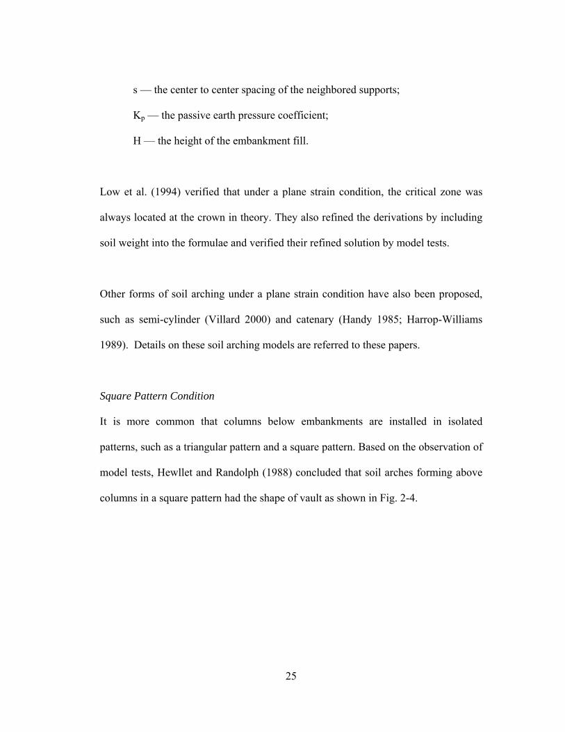
Square Pattern Condition

It is more common that columns below embankments are installed in isolated

patterns, such as a triangular pattern and a square pattern. Based on the observation of

model tests, Hewllet and Randolph (1988) concluded that soil arches forming above

columns in a square pattern had the shape of vault as shown in Fig. 2-4.

26

Fig. 2-4. Soil Arches above Column Grid of Square Pattern (Hewllet and Randolph 1988)

Different from the 2D condition, failure could occur either at the crown or at the

contact of the embankment fill and the column heads for a 3D condition. When the

height of the embankment fill, H, is relatively low as compared with the center-to-

center span of the columns, s, the failure at the crown governs. However, as the

embankment height is increased, the failure at the contact of the embankment fill and

the column heads controls. The above statement is consistent with the observation of

the penetration of columns into the embankment fill (Broms and Wong 1985).

Therefore, the soil arching ratio, ρ, can be expressed in two forms (the failure at the

crown and the failure at the contact):

27

(a) Failure at the crown

CABAE+−=

−−

= 211

δρ (2-5)

where E — efficacy of the columns, ))(1(1 2 CABAE +−−−= δ ;

sb /=δ ;

)1(2)1( −−= KpA δ ;

)3222

(2 −

−=

p

p

KK

HsB ;

)3222

(2 −

−−=

p

p

KK

HbsC .

(b) Failure at the contact of the embankment fill and the column heads

22 11

11

11

δβδρ

−⋅

+=

−−

=E (2-6)

where )]1()1[(1

11

2pp

p

p KKK

Kδδ

δβ +−−−×

+⋅

+= .

28

The case with the higher soil arching ratio dominates the actual situation. Chen et al.

(2004) suggested that the lateral earth pressure was less than Kp before the limit

equilibrium state was reached and a reduction coefficient, α, should be applied.

Hewllet and Randolph’s models are included in the German design methodology for

CS and GRCS embankments.

Finn’s Theory

Finn (1963) used continuum mechanics to solve an earth pressure distribution due to

soil arching under a 2D condition in terms of displacements (translation and rotation).

In his model, the soil does not reach the limit equilibrium state (i.e., soil is in an

elastic state) and the movement of the yielding base is either pure translation (Fig. 2.5

(a)) or pure rotation (Fig. 2.5 (b)). Any other forms of movement could be

approximated by a combination of pure translation and pure rotation. Finn (1960 and

1963) published analytical solutions for stresses induced by translation and rotation,

which are called Finn’s boundary value solutions. Finn’s solutions were well verified

against the existing data. To use Finn’s boundary value solutions, it is important to

ensure that soil is in an elastic state. However, Finn’s solutions contain singularity

points (x=y=0; x=b/x=-b, y=0) so that the integration of the stress values on the

displaced support becomes impossible. Consequently, Finn’s method cannot be used

to calculate the soil arching ratio.

29

2b

Rigid

Soil mass

d

h

y= ∞

Unit weight

2b

Rigid

Soil mass

d

h

y= ∞

Unit weight

(a) (b)

Fig. 2-5. Finn’s Pure Translation and Pure Rotation Models (Finn 1963)

A hypothesis was proposed to limit the maximum stresses at the singularity points to

obtain the integration of the induced stresses (Chelapati 1964). However, due to the

complexity of the problem, no analytical closed-form solution was obtained.

Numerical integration could be an alternative. However, it would likely be too time-

consuming even for a minor case (Getzler et al. 1968), therefore, it is not practical.

Another concern of Finn’s method is that the soil is treated as a linearly elastic

material. In reality, most soils have nonlinear stress-strain relationships.

30

Further Discussion on Soil Arching

Even though the soil arching phenomenon was identified more than a century ago,

due to its complexity, no comprehensive soil arching theory has been developed.

Ideally, a soil arching theory should be capable of considering the following four

factors, which primarily influence the development of soil arching (Terzaghi 1943;

Finn 1960; Gelzler et al. 1986): (1) the properties of the support (columns in this

study), especially its stiffness; (2) the properties of the soil medium, such as stiffness,

friction angle, density, etc.; (3) the geometry of the whole system, for instance, the

thickness of the soil medium, the dimension of the span, and the dimension of the

support; and (4) the boundary condition including a 2D or 3D problem, the

surcharge, and the allowable differential settlement.

Terzaghi (1943) assumed absolute rigid supports in his model. This assumption is

reasonable when the supports are much stiffer than the soil medium. In real

applications, however, some supports, such as stone columns, may not be that much

stiffer than the surrounding soil. The assumption of the rigid support may not be

valid for this kind of situation.

As demonstrated by all the theories except Finn’s, the friction angle of the soil affects

the efficiency of the load transfer. As Hewllet and Randolph (1988) pointed out, the

soil above the supports may yield first. Therefore, the better the soil, the more the

31

load transfer. However, Mckelvey III (1994) pointed out that the available theories

neglected classical geotechnical property, such as the change of volume under shear.

The geometry of the whole system has influence on the range and shape of soil

arching. For instance, Terzaghi (1943) concluded that the influence of soil arching

could extend vertically as high as 5 times of the clear span, while Hewllet and

Randolph (1988) found that the influence of soil arching would go to as high as the

clear span above the column heads. BS 8006 (BSI 1995) specified that the full soil

arching occurred at a height of 1.4 times the clear span.

As discussed earlier, differential settlement induces shear stresses in soil, which is the

intrinsic reason for soil arching. There is general agreement that the extent of soil

arching depends on the magnitude of differential settlement. The limit equilibrium

methods assume that yielding of the soil happens at or above the supports under

excessive differential settlement. Therefore, these soil arching theories typically

underestimate the soil arching ratio if the differential settlement is not high enough to

reach the limit equilibrium state.

32

2.2.2 Tensioned Membrane Theories

In general, a flexible sheet or membrane used to support a vertical load over a span is

referred as the “membrane effect”. In geotechnical engineering, geosynthetics are

often used as reinforcement to support a vertical load over a span, such as

geosynthetics over voids and geosynthetics over columns. Gourc and Villard (2000)

defined the “membrane effect” as “the ability of a geosynthetic sheet to be deformed,

thereby absorbing forces initially perpendicular to its surface tension.”

To quantify the membrane effect, a number of tensioned membrane models have been

proposed. Most of them were originally developed for the design of soil-geosynthetic

systems over voids (including tension cracks, sinkholes, dissolution cavities, and

localized depression). They have also been used in the design of GRCS embankments

recently. Among all the methods, Delmas’ (Delmas 1979), Giroud et al’s (Giroud et

al. 1990) and British Standard Method (BSI 1994) are the three most commonly used

tensioned membrane theories in geotechnical engineering.

Delmas’ Method

Delmas (1979) published an analytical method to calculate the tension deformation

developed in a horizontal sheet above a trench subjected to a uniformly distributed

vertical load as shown in Fig. 2-6 (a).

33

b

parabolic shapey

xq

b

parabolic shapey

xq

(a) Parabolic deformed layer (Delmas 1979)

y

b

circular shape

p y

b

circular shape

p

(b) Circular deflected membrane layer (Giroud et al. 1990)

Fig. 2-6. Delmas’ and Giroud’s Membrane Models

Delmas (1979) assumed that the load remained vertical and the deformed sheet had a

parabolic shape, which can be expressed as:

2 2

0 0

( )8 2qb qxY xT T

= − (2-7)

The maximum tension, Tmax, and the maximum deformation, ymax, can be calculated

as:

34

24 222

0max

bqTT

+= (2-8)

2

max08

qLyT

= (2-9)

where T0—the horizontal component of Tmax, which can be calculated using Eqs. (2-

10) and (2-11).

β20qbT = (2-10)

2

2

3]2)(1[3

βββββ

+−++

=ArgSh

JqL (2-11)

Giroud et al’s Method

Giroud et al. (1990) proposed another analytical solution to account for the membrane

effect. They assumed that the deformed membrane sheet had a circular shape and the

load acted normally to the deformed sheet as shown in Fig. 2-6 (b). They ignored the

friction between the soil and the membrane sheet to obtain a uniform strain

distribution.

The tension developed in a geosynthetic sheet over a 2D void (i.e., trench) can be

expressed in terms of a dimension factor, Ω:

35

Ω= pbT (2-12)

where T — the tension in the membrane;

p — the pressure normal to the membrane.

The dimension factor, Ω, is a piecewise function, which can be determined using Eqs.

(2-13) and (2-14) at a certain strain:

)21(sin21 1

ΩΩ=+ −ε ( 5.0/ ≤by ) (2-13)

)]21(sin[21 1

Ω−Ω=+ −πε ( 5.0/ ≥by ) (2-14)

where ε — the strain in the membrane;

y — the maximum deflection;

b — the width of the void.

Giroud et al’s method has been included in several design methodologies of GRCS

embankments.

As to the membrane above a circular void, Giroud et al. (1990) suggested that even

though the deflected shape was not a sphere, the diameter, 2r, should be used to

36

substitute the width, b, to obtain an approximate solution of the tension, T. Based on

Giroud et al’s method, the tension developed in the geosynthetic sheet is uniform.

However, experimental tests (Fluent et al. 1986; Rogbeck et al. 1998) and numerical

analysis (Han and Gabr 2002) have showed that the maximum strain occurred at the

edge of the columns.

British Standard Method

Different from Delmas’ (1979) and Giroud et al’s (1990) methods, the membrane

method included in BS 8006 (BSI 1995) was especially developed to design the

GRCS system. It was assumed that the weight of the presumed load is taken by the

reinforcement strips between the pile caps (i.e., the hatched area in Fig. 2-7) and the

load was distributed horizontally along the bridged span instead of the deformed

length, which led to a parabolic deformed shape but not a catenary shape (BSI 1995;

Agaiby and Jones 1995).

Fig. 2-7. Load Carrying Area of Geosynthetics

37

Then the tension developed in the geosynthetic reinforcement could be expressed as:

ε611

2+

−=

bbsWT T (2-15)

where s and b — the center to center spacing and the column size, respectively, as

shown in Fig. 2-7;

WT — the load to be taken by the geosynthetic;

ε — the strain in the geosynthetic.

Further Discussion on Tensioned Membrane Theories

A common drawback of these membrane theories discussed above is that the

compatibility of the tension and the strain developed in the geosynthetic

reinforcement is not necessarily satisfied. In addition, these methods neglected the

friction and confinement between the soil and the geosynthetic sheet, which is

important to the distribution of the tension.

Cautions should be paid when these membrane theories are used to estimate the

tension in geosynthetic reinforcement in GRCS embankments. Since these membrane

theories were developed based on the assumption that the geosynthetic reinforcement

is used to only support the vertical load over a trench or void, they did not account

38

for the portion of tension induced by the horizontal movement (such as the lateral

movement of the embankment fill) above the geosynthetic sheet. Jones et al. (1994)

and Horgan and Sarsby (2002) pointed out that the total tension generated in

geosynthetic sheet should be the sum of tension induced by vertical and horizontal

movements.

As mentioned earlier, basal reinforcement could have a single layer of geosynthetic or

multiple layers of geosynthetics. It has been debated that single-layer base

reinforcement may have different load transfer mechanisms from multiple-layer base

reinforcement (Collin 2003; Collin 2004; Huang et al. 2005). In the single layer

system, the single geosynthetic layer acts as a tensioned membrane. In the multiple-

layer system, however, the multiple geosynthetic layers and the fill material form a

load transfer platform, which acts similarly as a continuous beam/slab (Collin 2003;

Collin 2004; Huang et al. 2005). Obviously, a multiple layer system is more

complicated than a single layer system because it has more influence factors, such as

the number and spacing of geosynthetic layers. However, this study is only limited to

a single layer system, therefore, the discussion on the multiple layer system is beyond

the scope of this study.

39

2.3 Current Design Methodologies for GRCS Embankments

As a result of increased applications of GRCS embankments, a number of design

methodologies have been proposed in the past few years. All the design

methodologies were developed based on soil arching and tensioned membrane

theories. So far, they have considered soil arching and tensioned membrane effects

independently. During the design, a soil arching theory is first used to calculate the

load or pressure applied on the geosynthetic layer. Based on the assumed or estimated

strain level in the geosynthetic layer, the tension in the geosynthetic layer can be

calculated using a membrane theory. The commonly cited design methods include the

BS8006 Method (BSI 1995), the Swedish Standard Method (Carlson 1987; Rogbeck

et al. 1998), and the German Method (Kempfert et al. 2004). These design

methodologies are to be briefly reviewed below.

British Design Methodology (BSI 1995)

In this design methodology, the pressure to be taken by columns is calculated by Eq.

(2-16), which is a transform of Martson’s theory for positive projecting subsurface:

2[ ]c cp C bH Hγ

⋅= (2-16)

40

where Cc — the soil arching coefficient. 18.0/95.1 −= bHCc , for end-bearing piles;

07.0/5.1 −= aHCc , for friction and other piles;

pc — the pressure on columns;

H — the embankment height.

The above formula postulated that the least embankment height would be 1.4 times of

the clear spacing in order to fully mobilize the soil arching. In practice, the minimum

embankment height would be 0.7 times the clear spacing to mitigate local differential

settlements (SvanØ et al. 2000).

The weight, WT, taken by the reinforcement per unit length, would be expressed as:

2 2

2 2

1.4 ( ), 1.4( )( ),0.7( ) 1.4( )

c

fsT

fs q

ps b s f s b H s bHWs Hf f q s b H s bs b

γγγ

− ⎧ − > − ⎫⎪= ⎨ ⎬+ − ≤ ≤ −− ⎪ ⎭⎩ (2-17)

where WT—the distributed vertical load acting on the reinforcement between adjacent

pile caps;

ffs — the partial load factor for the soil unit weight;

fq — the partial load factor for the externally applied load;

q — the uniformly distributed surcharge.

41

On the basis of the calculated load to be taken by the geosynthetic, the tension

developed in the reinforcement is calculated using the membrane theory presented in

Eq. (2-15). Obviously, there exists a discontinuity if Eq. (2-17) is used to calculate the

load taken by the reinforcement (Rogbeck, and Gustavsson, et al. 1998).

Consequently, there must be a discontinuity in the calculated tension.

Swedish Design Methodology (Collin 2003)

For a two-dimensional case, Carlsson’s formula was used to calculate the load carried

by the geosynthetic as presented in Eq. (2-18).

2

0

( )4 tan15Ts bW γ−

= (2-18)

The membrane theory presented in Eq. (2-15) is used to calculate the tension in the

geosynthetic layer.

Both British and Swedish design methodologies neglect the subsoil support under the

geosynthetic reinforcement. However, numerical results from Jones et al. (1994)

showed that subsoil support is significant and could be as high as 80% of the

embankment load for a low embankment supported by widely spaced columns.

Rogbeck et al. (1998) also found that the subsoil resistance had noticeable influence

42

on the tension developed in the geosynthetic. Fluet et al. (1986) proposed a model

called a “fully flexible model”, which could consider subsoil resistance. However,

they did not provide any guidance on how to estimate the subsoil resistance.

German Design Methodology (Collin 2003)

The soil arching theory incorporated in the German design methodology is what

proposed by Hewlett and Randolph (1988). The vertical stress on the top of the

reinforcement is calculated for both two-dimensional and three-dimensional

situations. Unlike the British and Swedish design methodologies, the subsoil

resistance underneath the reinforcement is taken into consideration in this method.

The load taken by the geosynthetic is the difference between the load on the

reinforcement and the soil resistance beneath the reinforcement.

By assuming a factor of safety of 2, the subsoil resistance could be calculated as:

2)2(

0ucπ

σ+

= (2-19)

Where σ0—the stress on the lower surface of the reinforcement;

cu—the undrained shear strength of the subsoil.

43

Then the load taken by geosynthetic reinforcement is:

2 20( )( )

2( )s

Ts bW

s bσ σ− −

=−

(2-20)

The membrane theory presented in Eq. (2-15) is used to calculate the tension

developed in the geosynthetic layer. This design method is very similar to the

procedures described by Alzamore et al. (2000).

One of the basic differences from British and Swedish design methodologies is that

the German methodology accounts for subsoil resistance. Undoubtedly, the ignorance

of the subsoil resistance produces conservative results, which has been verified by

Rogbeck et al. (1998). However, whether the partial support of subsoil should be

considered is still under debate (Horgan and Sarsby 2002), since the support of

subsoil may decrease with the consolidation of soft soil.

Further Discussion on Design Methodologies

Besides the design methodologies presented above, there are several other design

methodologies. The design methodologies are distinguished from each other by the

soil arching theory and the membrane theory adopted. Since there are inherent

differences among soil arching theories and membrane theories, the consistency of

44

these design methodologies became the concern of practitioners. Several comparisons

have been done to evaluate the consistency of the design methodologies. However,

the investigations are inconclusive because remarkable differences have been found

among these design methodologies (Horgan and Sarsby 2002; Naughton and

Kempton 2005). Naughton and Kempton (2005) presented an extensive comparison

of soil arching ratios and tension in geosynthetic reinforcement obtained from a few

available analytical methods and they found large variations. Russell and Pierpoint

(1997) also presented a comparison based on two GRCS embankments. The basic

information on these two embankments (Embankments A and B) is provided in Table

2-1. The calculated soil arching ratios and tension in the reinforcement using different

methods are presented in Figs. 2-8 and 2-9, which show the soil arching ratio could

differ by more than three times while the tension could differ by more than two times.

Table 2-1. Information of Embankment A and B Used in Comparison (Russell and Pierpoint 1997)

Property Embankment A Embankment B

Height (m) 5.8 4.3 Pile cap width (m) 1.0 0.5 Pile spacing (m) 2.5 2.5 Longitude reinforcement stiffness (kN/m) 5500 294 Transverse reinforcement stiffness (kN/m) 9500 738 Fill Poisson’s ratio 0.2 0.2 Fill stiffness (MPa) 20 40 Average fill density (kN/m) 18.2 19.0 Fill angle of friction (o) 30 40 Fill dilation (o) 0 0 Fill cohesion (kPa) 0 10

45

Soil arching ratio, ρ

0

0.2

0.4

0.6

0.8

BS 8006 Terzaghi Hewlett &Randolph

Russel etal

Kempfertet al.

Embankment A

(a) Embankment A

Soil arching ratio, ρ

0

0.3

0.6

0.9

1.2

BS 8006 Terzaghi Hewlett &Randolph

Russel etal

Kempfertet al.

Embankment B

(b) Embankment B

Fig. 2-8. Soil Arching Ratio (Modified from Naughton and Kempton 2005)

46

Tension in reinforcement, T

0

50

100

150

200

250

BS 8006 Terzaghi Hewlett &Randolph

Russel etal

Kempfertet al.

Embankment A

(a) Embankment A

Tension in reinforcement, T

0

200

400

600

800

BS 8006 Terzaghi Hewlett &Randolph

Russel etal

Kempfertet al.

Embankment B

(b) Embankment B

Fig. 2-9. Tension in Geosynthetic Reinforcement (Modified from Naughton and Kempton 2005)

Researchers and designers have felt uncomfortable with these large variations among

different design methods, which have brought the uncertainty to the application of

47

GRCS embankments. To some extent, this uncertainty obstructs the wide acceptance

of GRCS embankments. For example, Collin (2004) suggested GRCS embankments

should not be built higher than 10m.

2.4 Current Research Status

In the past few years, a number of studies have been conducted to better understand

the mechanisms and behavior of GRCS embankments. These studies include

theoretical analyses, numerical modeling, field monitoring, full scale tests, and

laboratory tests. A few representative studies are summarized in Table 2-2.

Table 2-2. A Summary of Past Studies on GRCS Embankments

Type Brief description Reference

Numerical modeling

A numerical analysis was done to evaluate the reinforcing effect by varying column spacing, column modulus, and number of geogrid layers.

Ohkubo et al. 1996

Experimental and numerical

study

A physical model with columns in a square pattern was built in the lab. Influence of various factors (including properties of columns, properties of geosynthetic reinforcement, and height of embankment) on soil arching and surface settlements was addressed. 2D numerical modeling was also performed and the results were compared with test results.

Demerdash 1996

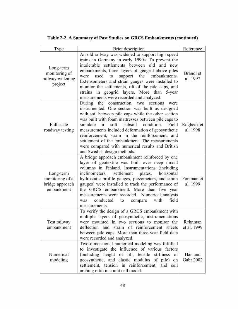
48

Table 2-2. A Summary of Past Studies on GRCS Embankments (continued)

Type Brief description Reference

Long-term monitoring of

railway widening project

An old railway was widened to support high speed trains in Germany in early 1990s. To prevent the intolerable settlements between old and new embankments, three layers of geogrid above piles were used to support the embankments. Extensometers and strain gauges were installed to monitor the settlements, tilt of the pile caps, and strains in geogrid layers. More than 5-year measurements were recorded and analyzed.

Brandl et al. 1997

Full scale roadway testing

During the construction, two sections were instrumented. One section was built as designed with soil between pile caps while the other section was built with foam mattresses between pile caps to simulate a soft subsoil condition. Field measurements included deformation of geosynthetic reinforcement, strain in the reinforcement, and settlement of the embankment. The measurements were compared with numerical results and British and Swedish design methods.

Rogbeck et al. 1998

Long-term monitoring of a bridge approach

embankment

A bridge approach embankment reinforced by one layer of geotextile was built over deep mixed columns in Finland. Instrumentations (including inclinometers, settlement plates, horizontal hydrostatic profile gauges, piezometers, and strain gauges) were installed to track the performance of the GRCS embankment. More than five year measurements were recorded. Numerical analysis was conducted to compare with field measurements.

Forsman et al. 1999

Test railway embankment

To verify the design of a GRCS embankment with multiple layers of geosynthetic, instrumentations were mounted in two sections to monitor the deflection and strain of reinforcement sheets between pile caps. More than three-year field data were recorded and analyzed.

Rehnman et al. 1999

Numerical modeling

Two-dimensional numerical modeling was fulfilled to investigate the influence of various factors (including height of fill, tensile stiffness of geosynthetic, and elastic modulus of pile) on settlement, tension in reinforcement, and soil arching ratio in a unit cell model.

Han and Gabr 2002

49

Table 2-2. A Summary of Past Studies on GRCS Embankments (continued)

Type Brief description Reference

Trial section of roadway widening

To confirm the design based on the numerical software-PLAXIS, a 200m long field trial section was built and instrumented. During the two months’ monitoring, traffic passed the trial section. Stresses on the piles and on the soil between piles were measured and analyzed.

Habib et al. 2002

Numerical modeling

Two-dimensional modeling was conducted to investigate the influence of various factors (including properties of subsoil, properties of embankment fill, properties of piles, and properties of geosynthetic) on settlement, tension in reinforcement, and soil arching ratio. In addition, slope stability analysis was conducted using a numerical approach and the results were compared with the limit equilibrium method.

Han and Shelth 2003

Full scale test

A 3m (width)×5m (length) test pit was built in Malaysia to investigate the load transfer mechanism of GRPS embankments. Steel piles were installed in a triangular pattern. Two layers of geotextile were placed. Load cells and Linear Variable Differential Transducers were mounted to monitor the deflection and the load transfer. Numerical modeling was conducted for comparison.

Chew et al. 2004

Analytical and

numerical study

Hewllet and Randolph’s arching theory was modified to calculate the tension in geosynthetic. Jia 2004

Numerical modeling

Extensive 2D and 3D axisymmetric numerical modeling was conducted to investigate the influence of various factors (including height of embankment, properties of embankment, tensile stiffness of geosynthetic, properties of pile, properties of subsoil, and even dilation of embankment fill) on the vertical load distribution among piles, geosynthetic reinforcement, and subgrade soil. Based on the findings from numerical modeling and compatibility analysis, an iteration approach to calculate the settlements, stresses on piles and tension in geosynthetic reinforcement was proposed.

Filz and Smith 2005

50

Even though the above studies have greatly improved our knowledge on GRCS

embankments, a number of limitations still exist as listed below:

♦ GRCS embankments are often a three dimensional problem since columns are

installed in an isolated pattern, such as a square or triangular pattern. Neither

axisymmetric analyses nor plane strain analyses can accurately represent the real

situation (Naughton and Kempton 2005).

♦ Unit-cell modeling cannot include the tension in the geosynthetic reinforcement

induced by lateral spreading (Han 2003).

♦ In most numerical modeling, two extreme states were analyzed: undrained and

drained. However, the settlement and tension development after construction are

more critical to the performance of the GRCS embankments, which have not been

well investigated.

♦ Laboratory tests have scale effects.

♦ Full-scale testing and long-term monitoring are ideal for research of GRCS

embankments. However, they are very time-consuming and costly. More importantly,

they are limited to specific test sites. Parametric studies are difficult to conduct.

51

♦ Little attention has been paid to the post-construction settlements, which are critical

to the serviceability of embankments.

To overcome the above limitations, this study was conducted in order to improve the

understanding of GRCS embankments. The full-scale embankments were numerically

modeled to eliminate the scale effect of unit cell modeling and small scale laboratory

tests. The mechanical and hydraulic models were coupled to frame the behavior of

GRCS embankments in a time domain to well evaluate the serviceability of the

GRCS embankments. The parametric study in 2D and 3D analyses investigated the

behavior of GRCS embankments under typical conditions in practice.

52

CHAPTER THREE

MODEL CALIBRATIONS

3.1 Introduction

To ensure the correctness of numerical models, they have to be calibrated against

available field data before they can be used for parametric studies. The calibrations

discussed below were conducted based on coupled mechanical and hydraulic

modeling of GRCS embankments using FLAC 2D and 3D software.

FLAC and FLAC3D are commercial two-dimensional and three-dimensional

software, respectively, which were developed by Itasca Consulting Group, Inc. The

finite difference software, FLAC (Fast Lagrangian Analysis of Continua) Version 4.0

developed by Itasca Consulting Group, Inc., was adopted in the two-dimensional

numerical study. The finite difference software, FLAC3D (Fast Lagrangian Analysis

of Continua) Version 3.1, also developed by Itasca Consulting Group, Inc., was

adopted in the three-dimensional numerical study.

Since GRCS embankments are usually built over soft soil with a high ground water

table, the generation and dissipation of pore water pressure (consolidation) during and

after construction are important for the behavior of GRCS embankments. This

behavior can be considered as an interaction of mechanical and hydraulic processes in

53

a time domain. FLAC and FLAC3D, capable of coupling mechanical and hydraulic

processes, were chosen to fulfill this goal. As hydraulic and mechanical modeling is

coupled, the mechanical and hydraulic loops are implemented alternately. In the

hydraulic loops, saturated transient fluid flow through porous media (soils) is

modeled to simulate the generation and dissipation of excess pore water pressures

(i.e., consolidation) during and after the construction. On the other hand, in the

mechanical loops, the stress and displacement development processes are modeled.

The two loops are coupled through the quasi-static Biot theory (Biot 1956). Starting

with a hydraulic loop, two variables (i.e., pore water pressure and specific discharge)

are evaluated by the transport law (Darcy’s law), the fluid mass balance law, and the

compatibility law. Then the change of pore water pressure is passed to the mechanical

loop to update the effective stress, which is used to check against failure and calculate

the volumetric strain based on the selected constitutive model. The calculated

volumetric strain is passed back to the hydraulic loop to account for the pore water

pressure and the specific discharge in the new hydraulic loop on the basis of the linear

quasi-static Biot theory (Itasca 2002), which is formulated in an incremental format.

As the two loops are implemented alternately, pore water pressures and volumetric

strains are kept exchanging and updating. The modeling of this process may require

thousands of cycles, which is terminated as a specified criterion (such as the

maximum unbalanced force, the flow time, the stress ratio and so on) is reached.

54

There are ten available constitutive models in FLAC and eleven constitutive models

in FLAC3D. Any of them can be used in the coupled mechanical and hydraulic

modeling to simulate the saturated soil behavior under stresses. In this study, soils

and deep mixed columns were modeled as linearly elastic perfectly plastic materials

with Mohr-Coulomb failure criteria in the mechanical modeling. The geosynthetic

layer was modeled using cable elements in FLAC 2D and geogrid elements in

FLAC3D, respectively. The numerical results based on the coupled mechanical and

hydraulic modeling are compared with the field measurements and those without the

hydraulic modeling.

3.2 Selected Case Study

A case history with fairly detailed material properties, necessary construction

information, and long-term settlement and tension monitoring data was selected from

the published literature (Forsman et al. 1999 and Forsman 2001) for the calibration

purposes.

The selected case study is a geosynthetic-reinforced DM column-supported

embankment built to support a new bridge approach over Sipoo River, Hertsby,

which is located about 30km northeast of Helsinki, Finland (Forsman et al. 1999).

The foundation soil from the ground surface downward consisted of 1 to 1.5m thick

55

crust, 10 to 14 m thick soft clay, 0 to 6m thick silt, and 1 to 5m thick glacial till. The

profile is presented in Fig. 3-1.

Fig. 3-1. Profile of Sipoo River Bridge Embankment (Forsman et al. 1999)

The index properties of the in-situ soils listed in Table 3-1 were reported by Forsman

et al. (1999). Oedometer and CPT tests indicated that the clay layer was normally

consolidated. The drained modulus Ed, the undrained modulus Eu, the drained

Poisson’s ratio νd, the effective friction angle φ′, and the effective cohesion c′ were

determined by triaxial tests, which are listed in Table 3-2. The ground water table was

close to the existing ground surface.

56

Table 3-1. Soil Index Properties

Depth (m) 4.8-5.6 10.5-11.3 15.9-16.3 Soil type soft clay soft clay silt Organic content (%) 0.8 0 0.7 Unit weight (kN/m3) 14.6-15.0 14.9-16.6 18.1-18.3 Water content (%) 80-91 58-85 31-41 Liquidity index (%) 91 84 31 Shear strength (CPT) (kPa) 6.5-16.1 8.7-15.2 13.9

Table 3-2. Properties of Soft Clay

Depth (m) Ed (kPa) νd Eu (kPa) cu (kPa) φ' (o) c′ (kPa) 4.9-5.7 300 0.1 3000-6000 12-17 13 8 10.6-11.2 600 0.2 4000-8000 0-15 13 8

The soft clay was considered to be the problematic layer. To minimize the

settlements, especially the crest (surface) settlements (also called post-construction

settlements), deep mixed (DM) columns were installed to improve the in-situ soils.

In addition, a layer of woven geotextile was placed over the DM columns as

geosynthetic basal reinforcement with a 0.3m thick cushion sand layer below. Each

DM column had a diameter of 0.8m and undrained shear strength of 150kPa. They

were alternately installed into two patterns (walls and isolated columns) parallel to the

centerline of the embankment as shown in Fig. 3-2. The isolated columns between

DM walls are referred as the mid-columns in this dissertation. The ultimate strength

of this geosynthetic reinforcement was 200kN/m in both longitudinal and transverse

directions. The secant tensile stiffness of this geosynthetic layer was 1790kN/m and

2120kN/m at strains of 2% and 6%, respectively. The adjacent geosynthetic sheets

57

were jointed together by seams. The soil stabilization was carried out by mixing soil

with cement and by-product binder at an amount of 130kg/m3 to form DM columns at

the beginning of 1996. After the ground improvement, the embankment with 2:1

(H:V) slopes on both sides was built successively in stages with a 0.50m thick sand

working platform, a 1.05m thick gravel sub-base, a 0.20m thick crushed stone base

course, and a 0.05m thick asphalt layer from 1996 to 1997. The geosynthetic layer

was installed within the working platform and 0.3m above the DM column heads.

The construction sequence is presented in Table 3-3. The embankment was

instrumented with piezometers, inclinometers, settlement plates, horizontal

hydrostatic profile gauges, and strain gauges on the geotextile sheet for construction

QC/QA and long-tern performance monitoring. However, only some of the settlement

and tension data were reported in the publications. The locations of the reported

hydrostatic profile gauges, settlement plates, and strain gauges are showed in Fig 3-3.

At Station 327.5 and Station 328.2, hydrostatic profile gauges were installed to

monitor settlements for transverse settlement profiles. Station 327.5 passes the mid-

span of the isolated columns, while station 328.2 passes the center of the isolated

columns. Settlement plates were mounted at locations of S1, S2, S3, and S4 to

monitor the settlements at the DM columns and at the soft soil. Strain gauges were

installed to monitor the strains in the geosynthetic sheet in two perpendicular

directions (the traffic and transverse directions). Representative points close to

Station 330.0 were presented here for comparison. The monitoring started at the same

time as the construction began and the data were kept updated up to five years after

58

the construction. The measured maximum settlement was approximately 120mm

(Forsman 2001). Differential settlement between the DM columns and soft soil was

observed. The settlements had become relatively stable after two years since the

construction. The measured strains in the geotextile in longitudinal and transverse

directions of the embankment were 0 to 0.2% and 0 to 1%, respectively. The tensions

in geotextile corresponding to 0.2% and 1% strain are 3.6kN/m and 18kN/m,

respectively.

1400 1400

8 x 1400

8500

Geosynthetic

DM column

Fig. 3-2. Embankment Cross-section and Column Layout (unit: mm) (Forsman et al. 1999)

59

Table 3-3. Construction Information

Stage No.

Material Thickness (m)

Duration (mm/yyyy—mm/yyyy)

1 Platform fill, sand 0.6 11/1996—01/1997 2 Embankment fill, gravel 0.9 01/1997—09/1997 3* Embankment fill +asphalt

layer 0.3 09/1997—03/1999

* Since no information available, it is assumed that traffic starts at this stage.

S2

S4

Center column wall

1m

S3

S1

Station 328.2

Station 327.5

(a) Locations of hydrostatic profile gauges

Station 330.0

B4B5

B7B8

Center column wall

A1A6

Station 330.0

B4B5

B7B8

Center column wall

A1A6

(b) Arrangement of strain gauges

Fig. 3-3. Arrangement of Instrumentations (Forsman 2001)

60

3.3 Numerical Modeling

To conduct the numerical model calibration, the selected case has to be converted into

numerical models. Due to the mid-columns, the selected case is a three-dimensional

problem. This case was modeled closely in the 3D calibration, while it was simplified

into two plane strain cases in the 2D calibration.

Soil is a stress-path dependant elastic-plastic material. To better simulate the actual

performance of the GRCS embankments, the construction procedure should be

closely modeled in the numerical analysis. In the actual stage construction, the

embankment was built to a pre-determined height for each stage at a certain

construction rate, which is typically represented by a linear slope as shown in Fig. 3-

4. After the pre-determined height was reached, the construction was temporarily

suspended to allow partial dissipation of excess pore water pressure and soft soil to

gain its strength. This time period is represented by a horizontal line in Fig. 3-4. Due

to the lack of the detailed construction procedure and the difficulty to simulate the

linear increase of the embankment height as shown in Fig. 3-4, the actual construction

process was approximated in the numerical model by a simplified construction

process as indicated by dash lines. In the simplified construction process, the

construction of each stage was completed instantly and then followed by a certain

period of waiting time for partial consolidation. The construction of the embankment

was modeled in three stages. The duration and the lift thickness of each stage were

61

determined based on the reported construction information and are schematically

presented in Fig. 3-5. The traffic was simulated by applying a distributed load of

12kPa on the crest of the embankment, which was assumed starting right after the

placement of the asphalt layer in Stage 3, i.e., the traffic loading was included in

Stage 3. After the completion of Stage 3 (i.e., 1.5 years after the service), the

modeling was extended to the end of the designed service life (30 years assumed in

this study) to predict the final crest settlements.

Load

Time

t1

ti

tn

Embankment construction Service

tc1 tw1 tci twi tcn twn

h1

hi

hn

Load

Time

t1

ti

tn

Embankment construction Service

tc1 tw1 tci twi tcn twn

h1

hi

hn

Fig. 3-4. Construction Process

Time

Load

2 month 8 month 18 month

0.6m

0.9m

0.3m

+tra

ffic

30 years

Time

Load

2 month 8 month 18 month

0.6m

0.9m

0.3m

+tra

ffic

30 years

Fig. 3-5. Modeling Procedure

62

3.4 Two-dimensional (2D) Model Calibration

In the numerical analysis, DM columns, soft soil, firm soil, and embankment fill were

modeled as linearly elastic perfectly plastic materials with Mohr-Coulomb failure

criteria, i.e., Mohr-Coulomb materials. The geosynthetic reinforcement was modeled

as a system of built-in cable elements, which could take axial tensile load only.

3.4.1 Numerical Modeling

The two-dimensional (2D) numerical model for this calibration study is presented in

Fig. 3-6. Due to the symmetry of the problem, only half of the section was modeled in

the calibration to save the computing time. The DM columns with a wall pattern were

represented by two-dimensional DM walls with an effective thickness of 0.7m. The

effective thickness was estimated based on the equivalency of the actual area of a

series of DM columns to the area of the wall modeled in the analysis. The wall at the

centerline had only half-width, i.e., 0.35m. The elastic modulus of the DM columns

was estimated based on the typical relationship of E = 100qu (Porbaha 2000 and

Bruce 2001), where qu = the unconfined compression strength (i.e., 300kPa in this

study).

63

The existence of mid-columns made it a three-dimensional problem. To convert the

three dimensional problem to a two-dimensional one, two simplified cases were

investigated: (1) without the mid-columns (referred as SC1 in this dissertation), i.e.,

ignore the existence of the mid-columns, which may be the worst situation for design

and (2) with the mid-columns (referred as SC2 in this dissertation), but each row of

mid-columns and soft soil between were converted to an equivalent DM wall. In the

CS2 case, the wall thickness for the mid-columns was taken to be the same as the

column walls but the equivalent elastic modulus and the equivalent cohesion of the

mid-column walls were determined based on the weighted area average of these

properties from the DM columns and the soft soil between as indicated by the dash

lines in Fig. 3-6. For instance, the equivalent elastic modulus and cohesion of the

middle DM walls are )a1(EaEE sssceq −+= and )a1(cacc sssceq −+= , where Ec

and Es are the moduli of the mid-DM columns and the soft clay, respectively; cc, and

cs are the cohesion of the column and the soft soil, respectively; as is the area

replacement ratio, defined as the ratio of the column area to the total area.

64

15 m 2.8 m 2.8 m

0.7 m 15 m

2.0 m

1.8 m1 2

12kPa

Geosynthetic

Soft clay

Silt

DM columns

Embankment fill

Fig. 3-6. 2D Numerical Model

The DM walls, the converted mid-DM walls, the soft clay, the silt, and the

embankment fill were modeled as linearly elastic-perfectly plastic materials with

Mohr-Coulomb failure criteria. DM columns extended to the depth of the firm glacial

soil. No deformation below the silt layer was assumed. Cable elements incorporated

in the software, which can only sustain axial tension, were used to simulate the

geotextile layer. The geosynthetic layer was located 0.3m above the top of the DM

columns. The properties of the DM walls, the converted mid-DM walls, the soft clay,

65

the silt, the embankment fill, and the geosynthetic layer are provided in Table 3-4,

most of them from Forsman et al. (1999). The properties of the crust at the ground

surface were not available and treated as part of the soft clay in the numerical analysis

to account for the disturbance of the surface layer during construction.

Table 3-4. Material Properties

Material E (MPa)

ν γ (kN/m3)

c′ (kPa)

φ' (o)

w (%)

k (m/s)

Soft soil 0.3 0.2 10.0* 8 13 70% 6.342×10-11 Silt 1.6 0.33 15.4* 5 20 70% 6.342×10-11

Embankment fill (base course) 40 0.33 20 5 38 N/A N/A

Platform fill (sub-base layer) 20 0.33 20 5 32 N/A N/A

DM walls 30 0.3 20 150 0 30% 6.342×10-11 Converted

mid-DM walls 15 0.3 20 79 0 30% 6.342×10-11

Geotextile J=1700kN/m, ci=0.8, ks=85,000kN/m/m Note: E = elastic modulus, ν = Poisson’s ratio, γ = unit weight, c’ = effective cohesion, φ′ = effective friction angle, w = water content, k = permeability, J = tensile stiffness of geotextile, ci = interaction coefficient between geotextile and sand, and ks = interface shear stiffness between geotextile and sand. The unit weight with a symbol ‘*’ is the dry unit weight, which was calculated based on the actual water content and the assumed specific gravity of 2.7. In the modeling of water flow in FLAC, the dry unit weight needs to be assigned to any material below the ground water table.

The FLAC models of these two cases are presented in Fig. 3-7 (a) and (b),

respectively.

66

(a) SC1

(b) SC2

Fig. 3-7. FLAC Models

67

3.4.2 Results and Comparison

In the numerical modeling, pore water pressure, effective stress, settlement, and

tension in the geosynthetic layer were recorded. Due to the limited availability of the

field measured data, only settlements and strains in the geosynthetic layer at certain

locations are compared with the field data.

Settlement

The settlements at the base of the embankment were monitored by horizontal

hydrostatic profile gauges at Station 327.5 and Station 328.2, as shown in Fig. 3-3 (a)

(Forsman 2001). Settlements at selected locations (S1, S2, S3, and S4) as shown in

Fig. 3-3 (a) were measured by settlement plates and reported from the beginning of

the construction. As mentioned in the case description, the measured settlement

profiles at Station 327.5 were at the cross-section without isolated columns, while the

measured settlement profiles at Station 328.2 were at the cross-section with isolated

columns. Therefore, the measured settlement profiles at Station 327.5 and the

measured time-settlement curves at S1 and S2 were compared with the numerical

results from the SC1 case, while the measured settlement profiles at Station 328.2 and

the measured time-settlement curves at S3 and S4 were compared with the numerical

results from the SC2 case.

68

0

40

80

120

160

0 2 4 6 8Distance from the toe (m)

Settl

emen

t (m

m)

Stage 1 (measured)Stage 2 (measured)Stage 3 (measured)Stage 1 (calculated)Stage 2 (calculated)Stage 3 (calculated)

(a) Measured settlement profiles at Station 327.5 and profiles from SC1

0

40

80

120

160

0 2 4 6 8Distance from the toe (m)

Settl

emen

t (m

m)

Stage 1 (measured)Stage 2 (measured)Stage 3 (measured)Stage 1 (calculated)Stage 2 (calculated)Stage 3 (calculated)

(b) Measured settlement profiles at Station 328.2 and profiles from SC2

Fig. 3-8. Settlement Profiles at Different Stages (2D)

69

Fig. 3-8 shows that the settlement profiles from the SC1 case match the

measurements at Station 327.5 reasonably well but the settlement profiles from the

SC2 case underestimated the measurements at Station 328.2. Similarly, the SC1 case

can fairly well capture the trend of the measured settlements at S1 and S2, however,

the SC2 case underestimated the measured settlements at S3 and S4, as shown in Fig.

3-9.

0

20

40

60

80

100

120

140

0 10 20 30 40 50 60Time (mon)

Settl

emen

t (m

m)

S1 (measured)S2 (measured)S1 (calculated)S2 (calculated)

(a) Settlements at S1 and S2

Fig. 3-9. Settlement versus Time (2D)

70

0

20

40

60

80

100

120

140

0 10 20 30 40 50 60Time (mon)

Settl

emen

t (m

m)

S3 (measured)S4 (measured)S3 (calculated)S4 (calculated)

(b) Settlements at S3 and S4

Fig. 3-9. Settlement versus Time (2D) (continued)

Han et al. (2005) conducted a numerical study on the SC1 and SC2 cases under a

drained condition (i.e., mechanical modeling with drained moduli). The maximum

settlements from the drained analysis, which occurred at the base of the embankment,

are presented in Table 3-5 for the comparison with those from the coupled analyses at

30-year service life. It is shown that the maximum settlement values from the drained

analysis are always greater than those from the coupled analysis.

71

Table 3-5. Maximum Settlements at the Base of the Embankment

Numerical analysis SC1 SC2

Coupled Drained Coupled DrainedMaximum settlement between DM walls

(mm) 131 196 94 110

Maximum settlement on DM walls (mm) 109 127 87 100

Even though the settlements on the crest were not measured in the field, it is very

important to investigate them since they are more critical to the performance of the

embankment. Fig. 3-10 presents the calculated settlement profiles at the base, as well

as those at the crest of the embankment, at the end of Stage 3 and at the 30-year

service life using the coupled numerical modeling. It is shown that the maximum

settlement at the crest is about 1/3 to 1/4 that at the base of the embankment. Obvious

differential settlement occurs at the base of the embankment between DM walls,

whereas this local differential settlement does not exist on the crest. Even though the

maximum settlement occurs at the base of the embankment, the post-construction

settlement at the crest of the embankment is crucial for the serviceability of

pavements on embankments or the connection between approach embankments and

bridge abutments. The settlement at the crest of the embankment starts to accumulate

right after the placement of the asphalt layer; therefore, it is actually the post-

construction settlement.

72

0

30

60

90

120

150

180

0 2 4 6 8Distance from the toe (m)

Settl

emen

t (m

m)

at end of Stage 3 (crest)at the end of service life (crest)at the end of Stage 3 (base)at the end of service life (base)

(a) Settlement profiles of SC1

0

30

60

90

120

150

180

0 2 4 6 8Distance from the toe (m)

Settl

emen

t (m

m)

at end of Stage 3 (crest)at the end of service life (crest)at end of Stage 3 (base)at end of service life (base)

(b) Settlement profiles of SC2

Fig. 3-10. Settlement Profiles at the Base and on the Crest of the Embankment (2D)

73

Fig. 3-10 also shows that the SC2 case has less settlement than the SC1 case because

the SC2 case has additional mid-DM walls between the regular DM walls. The post-

construction settlement further increases from the end of Stage 3 to the 30-year

service life.

Strain and Tension in Geosynthetic Layer

Strain gauges were installed near Station 330.0 to monitor the development of strains

at different locations as shown in Fig. 3-3 (b) (Forsman 2001). Since B7 and B8 were

located along the cross-section without isolated columns, their measurements were

compared with results from the SC1 case as shown Fig. 3-11 (a). Since B4 and B5

were located along the cross-section with isolated columns, their measurements were

compared with results from the SC2 case as shown in Fig. 3-11 (b). Good agreement

was found between field measurements and results from the SC1 case at B7 and B8.

But results from the SC2 case underestimated the measurements at B4 and B5. This

finding is consistent with what has been found in the settlement comparison.

74

0

0.2

0.4

0.6

0.8

1

1.2

1.4

1.6

0 20 40 60Time (mon)

Stra

in (%

)

B7 (measured)B8 (measured)B7 (calculated)B8 (calculated)

(a) Strains at B7 and B8

0

0.2

0.4

0.6

0.8

1

1.2

1.4

1.6

0 20 40 60Time (mon)

Stra

in (%

)

B4 (measured)B5 (measured)B4 (calculated)B5 (calculated)

(b) Strains at B4 and B5

Fig. 3-11. Strain versus Time (2D)

75

The profiles of tension developed in the geosynthetic layer from the coupled

numerical analysis for the SC1 and SC2 cases are presented in Fig. 3-12. It is shown

that the higher tension is located above the DM columns, which is consistent with the

findings from the field measurements and the earlier study on a unit cell model by

Han and Gabr (2002). The tension in the reinforcement above the mid-DM walls is

lower than that above other DM walls. This phenomenon is attributed to the fact that

the equivalent modulus of the mid-DM walls is lower than that of other DM walls.

Overall, the tension in the reinforcement for the SC1 case is higher than that for the

SC2 case. This result is intuitively correct since the mid-DM columns in the SC2

case minimize the tension in the reinforcement.

0

4

8

12

16

20

0 2 4 6 8

Distance from the toe (m)

Tens

ion

(kN

/m)

SC1SC2

column

mid-column

Fig. 3-12. Tension Developed in the Geosynthetic Layer with or without Mid-DM Walls

76

Table 3-6 presents the measured tension range of the calculated results using coupled

and drained numerical models. Both numerical models for the SC1 case yield the

close result for the tension in the geosynthetic layer, whereas those for the SC2 case

underestimate the tension in the reinforcement. This comparison can be explained

that the maximum span of the geosynthetic sheet in the field is that between two DM

walls not between the mid-DM columns and the DM wall since mid-DM columns

have gaps in the centerline direction. The case for the geosynthetic sheet across two

DM walls is the case of SC1.

Table 3-6. Maximum Tension in the Geosynthetic Layer

Numerical analysis SC1 SC2

Measured Coupled Drained Coupled Drained Tension (kN/m) 3.6 -18.0 1.5 - 17.8 1.9 - 18.3 1.5 - 7.8 1.8 - 7.3

On the completion of the 2D model calibration, 3D model calibration was conducted

on the same case history with the same modeling procedure as 2D.

3.5 Three-dimensional (3D) Model Calibration

Similar to the 2D model calibration, DM columns, soft soil, firm soil, and

embankment fill were modeled as Mohr-Coulomb materials in the 3D model

77

calibration. The geosynthetic reinforcement was modeled as built-in geogrid

elements, which are plane triangular elements and can take axial load only.

3.5.1 Numerical Modeling The three-dimensional (3D) numerical model for this case study is presented in Fig.

3-13. And the elevation view and plan view of the FLAC3D model are presented in

Fig. 3-14 (a) and (b), respectively.

To save computing time, only half span in the traffic direction was modeled. For

simplicity, the DM column walls and isolated DM columns were simplified to

rectangular and square shape, which have effective thickness and effective size of

0.7m and 0.7m, respectively. The material properties used are the same as those used

in 2D (refer to Table 3-4).

The modeling procedure in the 3D analysis is the same as that in the 2D analyses.

78

15 m 2.8 m 2.8 m

0.7 m15 m

2.0 m

1.8 m12

12kPa

Geosynthetic

Soft clay

Silt

DM columns

Embankment fill

0.7m

15 m 2.8 m 2.8 m15 m 2.8 m 2.8 m

0.7 m15 m

2.0 m

1.8 m12

12kPa

Geosynthetic

Soft clay

Silt

DM columns

Embankment fill

0.7m

Fig. 3-13. 3D Numerical Model

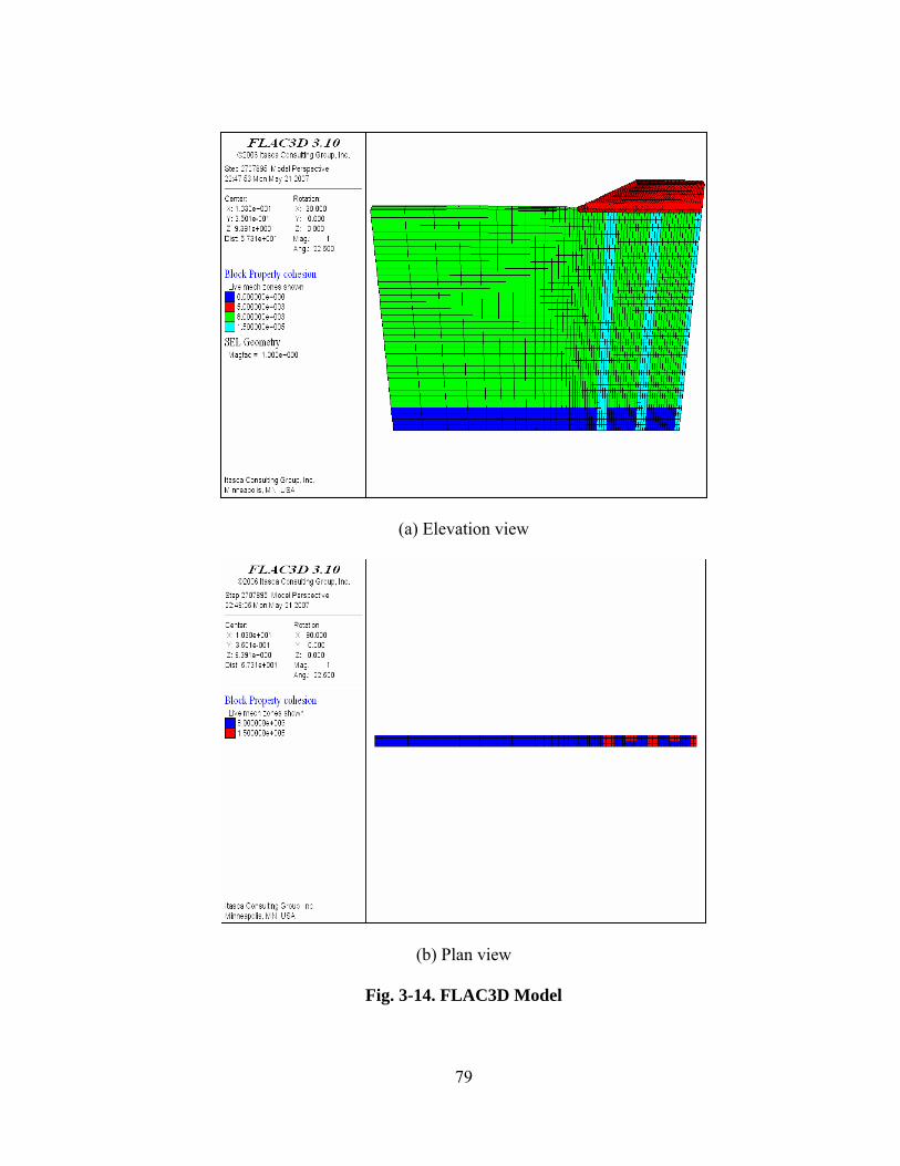
79

(a) Elevation view

(b) Plan view

Fig. 3-14. FLAC3D Model

80

3.5.2 Results and Comparison

In the numerical modeling, pore water pressure, effective stress, settlement, and

tension in both traffic and transverse directions were recorded. Settlements and strains

in geosynthetic at certain locations are compared with field data below.

Settlement

The settlement profiles at Station 327.5 and Station 328.2 based on the measurements

by hydrostatic profile gauges are compared with 3D numerical results in Fig. 3-15.

0

20

40

60

80

100

120

140

160

0 2 4 6 8Distance from the toe (m)

Settl

emen

t (m

m)

Stage 1 (measured)Stage 2 (measured)Stage 3 (measured)Stage 1 (calculated)Stage 2 (calculated)Stage 3 (calculated)

(a) Measured and calculated settlement profiles at Station 327.5

Fig. 3-15. Settlement Profiles at Different Stages (3D)

81

0

20

40

60

80

100

120

140

160

0 2 4 6 8Distance from the toe (m)

Settl

emen

t (m

m)

Stage 1 (measured)Stage 2 (measured)Stage 3 (measured)Stage 1 (calculated)Stage 2 (calculated)Stage 3 (calculated)

(b) Measured and calculated settlement profiles at Station 328.2

Fig. 3-15. Settlement Profiles at Different Stages (3D) (continued)

It can be found that numerical analysis provided reasonably good prediction,

especially at Stage 3 at Station 327.5. Even though deviations exist between

measurements and numerical results at Stage 1 and Stage 2, the numerical analysis

can capture the trend of the development of the settlement across the sections.

In addition, the settlements monitored by the settlement plates at S1, S2, S3 and S4

(refer to Fig. 3-3 (a)) were also compared with the 3D numerical results in Fig. 3-16.

Similarly, the 3D numerical results slightly overestimate the field measurements at

82

Stage 1 and Stage 2 at S1, S2, S3, and S4. Nevertheless, it yields fairly good

agreement on the final settlements at those four locations.

0

20

40

60

80

100

120

140

0 10 20 30 40 50 60Time (mon)

Settl

emen

t (m

m)

S1 (measured)S2 (measured)S1 (calculated)S2 (calculated)

(a) Settlements at S1 and S2

0

20

40

60

80

100

120

140

0 10 20 30 40 50 60Time (mon)

Settl

emen

t (m

m)

S3 (measured)S4 (measured)S3 (calculated)S4 (calculated)

(b) Settlements at S3 and S4

Fig. 3-16. Settlement versus Time (3D)

83

The settlement profiles from the numerical analysis at the crest and at the base are

presented in Fig. 3-17. Due to the computing time, the 3D numerical analysis was

only implemented up to ten years after service. Based on the settlement increment

from at the end of Stage 3 to ten years after service, it can be anticipated that the

settlement increment from 10 years to 30 years after service will be small.

Apparently, the post-construction settlements at the crest are much less than those at

the base. More importantly, the local differential settlements between columns and

soft soil at the base are not directly reflected to the crest.

0

30

60

90

120

150

0 2 4 6 8Distance from the toe (m)

Settl

emen

t (m

m)

at the end of Stage 3 (crest)10 years after service (crest)at the end of Stage 3 (base)10 years after service (base)

Fig. 3-17. Settlement Profiles on the Crest and at the Base (3D)

84

Strain and Tension in Geosynthetic Layer

As mentioned previously, strain gauges were installed near Station 330.0 to monitor

the development of strains at different locations (refer to Fig. 3-3). The computed

strains at two locations in each direction, i.e., B4 and B5 in the transverse direction

and A1 and A6 in the traffic direction, were compared with measured results as

shown in Fig. 3-18. It was found that at B4 and B5 the numerical results were less

than the measurements. The computed strains along the traffic direction at two

locations (A1 and A6) are also less than measurements. The deviation between

calculation and measurements may be attributed to the properties used in the

modeling. The properties used in the modeling were based on short-term laboratory

tests, while the field performance was a long-term behavior.

It is a common knowledge that the settlement measurements in the field are more

accurate and reliable than strain measurements (Dunnicliff 1988).

Overall, it can be concluded that the 2D and 3D models can reasonably predict the

performance of GRCS embankments in the field as demonstrated for this selected

case history. The 2D and 3D model calibrations ensure the basis for the following

parametric studies.

85

0

0.2

0.4

0.6

0.8

1

1.2

1.4

1.6

0 10 20 30 40 50 60Time (mon)

Stra

in (%

)B4 (measured)B5 (measured)B4 (calculated)B5 (calculated)

(a) Strain at B4 and B5

0

0.5

1

1.5

2

2.5

3

0 10 20 30 40 50 60Time (mon)

Stra

in (%

)

A1 (measured)A6 (measured)A1 (calculated)A6 (calculated)

(b) Strain at A1 and A6

Fig. 3-18. Strain versus Time Relationship (3D) (continued)

86

CHAPTER FOUR

TWO-DIMENSIONAL PARAMETRIC STUDY

On the basis of the model calibration, a two-dimensional (2D) parametric study was

conducted to investigate the influence of key factors on total settlements, differential

settlements, tension developed in geosynthetic reinforcement, stress concentration

ratio, and excess pore water pressure generation and dissipation.

4.1 2D Baseline Case

A baseline case was first selected as a typical case in the field and analyzed to

develop a basis for comparisons when parameters were deviated from the baseline

base. The deviations of the parameters were considered to cover their typical ranges

in most actual projects.

4.1.1 2D Dimensions and Properties

To make the results comparable, a baseline case was determined based on a typical

configuration. The dimensions and properties are presented in Fig. 4-1 and Table 4-1,

respectively.

87

Soft clay

Firm soil

DM column

10m

5m

2m

1m

1.5m

0.25m

40m 10m10m

Fill

12kPa

z

X

AB

B′ A′

CD

E

I

I

Soft clay

Firm soil

DM column

10m

5m

2m

1m

1.5m

0.25m

40m 10m10m

Fill

12kPa

z

X

AB

B′ A′

CD

E

I

I

Fig. 4-1. Two-dimensional Model of the 2D Baseline Case

Due to its symmetry, only half of the embankment was modeled to save computing

time as shown in Fig. 4-1. The embankment slope was assumed to be 2:1 (H:V),

which is widely adopted in practice. The height of the embankment was 5m. Half

width of the crest, equal to 10m, was selected based on a two-lane highway in each

direction plus a shoulder. The in-situ soils below the embankment included a layer of

10m thick soft clay and a layer of 2m thick underlying firm soil. The DM columns

were assumed to penetrate 1m into the firm soil. No settlement was allowed below

the firm soil layer to simulate the underlying bedrock. A geosynthetic layer was

placed 0.25m above the heads of the columns. The end of the geosynthetic sheet at

the centerline was fixed laterally but free vertically and the end toward the toe was

88

free in both directions. The boundary effect was eliminated by extending the left

boundary of the model far enough from the toe of the embankment. The traffic load

was simulated by applying a uniformly distributed load of 12kPa on the crest of the

embankment. The ground water level was assumed at the ground surface.

Table 4-1. Properties of Materials in the 2D Baseline Case

Material Properties

DM columns γ = 18kN/m3, c = 500kPa, φ′ = 0o, E = 100MPa, ν = 0.3, ct = 100kPa, k = 1×10-9m/s

Soft Soil γ = 18kN/m3, c' = 0kPa, φ′ = 25o, E = 2MPa, ν = 0.3, ct = 0kPa, k = 1×10-9m/s

Firm Soil γ = 18kN/m3, c′ = 0kPa, φ′ = 30o, E = 100MPa, ν = 0.3, ct = 0kPa, k = 1×10-9m/s

Embankment Fill γ = 18kN/m3, c′ = 5kPa, φ' = 32o, E = 30MPa, ν = 0.3, ct = 0kPa

Geosynthetics t = 0.002m, Er = 500MPa, Ta = 100kN/m, ks = 20MN/m/m, ca = 0kPa, δ = 24.8o

Ground water K = 200MPa Note: γ = unit weight of soil; c = shear strength of soil-cement; c′ = effective cohesion of soil; φ′ = effective friction angle of soil; k = permeability; E = elastic modulus of soil; ν = Poisson’s ratio; ct = tensile strength of soil-cement/soil; t = thickness of geosynthetic reinforcement; Er = elastic modulus of geosynthetic reinforcement; Ta = allowable tensile strength of geosynthetic reinforcement; ks = bond stiffness between geosynthetic and embankment fill; ca = bond strength between geosynthetic and embankment fill; δ = bond friction angle between geosynthetic and embankment fill; K = water bulk modulus.

The properties of DM columns, soft soil and embankment fill of the baseline case

were in the middle of their typical ranges to leave enough margins for property

variations in the parametric study (EPRI 1990; Budhu 2000). The shear strength of

DM columns was determined from the common correlation of cE ⋅= 200 (Bruce

2001), where c is the undrained shear strength of DM columns and equal to half of

the unconfined compressive strength. In addition, the DM columns were assumed to

89

have a tensile strength, ct, equal to 20% of the undrained shear strength, c. The pure

water bulk modulus is 2GPa. However, since the natural ground water includes

dissolved air and some trapped air bubbles, which greatly increase the compressibility

of the ground water, a reduction factor of 0.1 was applied to the pure water bulk

modulus to obtain the ground water bulk modulus, K, as suggested by Itasca (2002).

A typical reduction factor 0.8 was applied to the soil-geosynthetic interface strength

as compared with the soil strength. Unsaturated flow was not modeled in this study.

Therefore, the pore water pressure at and above the ground water surface was always

fixed at zero. The right boundary in Fig. 4-1 was assumed to be impervious, i.e., no

water enters or leaves the plane of symmetry. The left boundary was also assumed to

be impervious since it was far enough away from the embankment and would not

make any influence on the numerical results.

4.1.2 2D Modeling Procedure

The modeling can be divided into three phases according to the execution sequence:

the generation of the initial ground stress field and the hydrostatic pore water

distribution, the simulation of the embankment construction, and the application of

the traffic load. Among all the phases, the simulation of the embankment construction

is the key to the modeling. The basic modeling procedure is listed in Table 4-2.

90

Table 4-2. Modeling Procedure

Phase Procedure Description

1 Initial condition Generate the initial stress field in the ground and the hydrostatic pore water pressure below the ground water table

Stage 1 Install DM columns and geosynthetic reinforcement, build the embankment to 1m high and allow the consolidation for 1 month

Stage 2 Build the embankment to 2m high and allow the consolidation for 1 month

Stage 3 Build the embankment to 3m high and allow the consolidation for 1 month

Stage 4 Build the embankment to 4m high and allow the consolidation for 1 month

2 Construction of embankment

Stage 5 Build the embankment to 5m high and allow the consolidation for 1 month

3 Traffic load Apply a traffic load of 12kPa and allow the consolidation up to 30 years

The construction of the embankment over soft soil was in stages (i.e., staged

construction) to ensure its stability and minimize its post-construction settlement. The

basic concept of staged construction has already been discussed in Chapter Three and

is schematically presented in Fig. 4-2. The required waiting time depends on several

factors, such as the permeability, the depth of the ground water table, the shear

strength of soft soil, the embankment height, the drainage conditions and so on.

Similarly as the model calibration, a simplified procedure was followed in this study

as shown in Fig. 4 (b), which is often used in design. In this study, the 5m high

embankment was constructed in five stages of equal thickness, i.e., the thickness of

each lift was 1m. To keep consistent with common practice, the duration of each

stage was 1 month (30 days). The traffic load was applied 1 month after the

91

completion of the embankment. The coupled modeling was lasted up to 30 years after

the service to simulate the typical service life of highways before major maintenance.

Embankment height

Time

(a) Actual process

Embankment height

Time

(b) Simplified process

Fig. 4-2. Modeling of Staged Construction

92

4.1.3 Results of 2D Baseline Case

Settlement

The settlement contour of the baseline case at 1 month after service is presented in

Fig. 4-3. The unit of the settlement is meter. It can be seen that the maximum

settlement developed at the base of the embankment. Apparent differential settlement

also developed at this elevation because of the stiffness and strength difference

between DM columns and soft soil.

Fig. 4-3. Settlement Contour of the 2D Baseline Case

93

The development of settlements at two locations, A and B (refer to Fig. 4-1), is

presented in Fig 4-4. In each stage, the settlement was accumulated with a sudden

increase, which indicated the immediate settlement at the completion of each stage.

After each sudden increase, the settlement increased gradually due to the process of

consolidation. As shown in Fig. 4-4 (b), the settlement became stable after

approximately 20 months after service, which is much shorter than that predicted

using Terzaghi’s one-dimensional consolidation theory. The consolidation process of

the column-supported embankment will be discussed in the excess pore water

pressure section.

0

10

20

30

40

50

0 2 4 6Time (mon)

Settl

emen

t (m

m)

Point APoint B

(a) 1 month after service

Fig. 4-4. Settlement versus Time of the 2D Baseline Case

94

0

10

20

30

40

50

0 100 200 300 400Time (mon)

Settl

emen

t (m

m) Point A

Point B

(b) 30 years after service

Fig. 4-4. Settlement versus Time of the 2D Baseline Case (continued)

However, since in the numerical analysis, the embankment was built to a pre-

determined elevation rather than a total thickness, the settlement occurring in the

previous stage was leveled off in the following stage. As a result, the settlement on

the crest of the embankment occurred after the completion of construction, which is

often called the post-construction settlement. The post-construction settlement of the

GRCS embankment system is more crucial to the performance of the pavement on the

embankment or the connection between the approach embankment and the bridge

abutment than the total settlement at the base of the embankment. The settlement on

the crest, Sp, can be expressed as follows:

ssctitccp SSSSS +++= (4-1)

95

where Sp = the settlement at the crest up to the designed service life, Scc = the

settlement due to the dissipation of the excess pore water pressure accumulated

during the construction, Sit = the immediate settlement due to traffic load, Sct = the

settlement due to the dissipation of the excess pore water pressure induced by the

traffic load within the designed service life, and Sss = the secondary settlement due to

the creep of soft soils, which is not included in this study.

Another fact worthy of being pointed out is that in this study the pavement was

modeled as part of the last stage of the embankment construction, therefore, the

settlement on the crest started to accumulate as long as the last stage of the

embankment (the 5th stage) was constructed. Sit was the immediate settlement

induced by the last stage of the embankment load and the traffic load in this study.

The settlements on the crest and at the base of the embankment at different time

periods are presented in Fig. 4-5. It can be seen that the maximum settlements at the

base were much larger than those on the crest at the same time. In addition, at the

base of the embankment, the soft soil between the DM columns settled much more

than the DM columns, therefore, the differential settlements at this elevation were

much more obvious than those on the crest.

96

0

10

20

30

40

50

60

70

0 5 10 15 20Distance from the toe (m)

Settl

emen

t (m

m)

1 month after service (crest)30 years after service (crest)1 month after service (base)30 years after service (base)

Fig. 4-5. Settlement Profiles of the 2D Baseline Case at Different Time

Differential settlements, especially those on the crest, are even more critical, because

they can induce cracks on the pavement, which affect the serviceability of the

pavement.

In this study, the differential settlement is defined as the absolute settlement

difference between the peak and the adjacent valley as illustrated in Fig. 4-6. Another

important parameter reflecting the degree of differential settlement is called the

distortion, which is defined as:

i

ii L

ssI

Δ= (4-2)

97

where Δssi – the differential settlement, i.e., the absolute settlement difference

between the peak and the adjacent valley;

Li – the distance between the peak and the valley as shown in Fig. 4-6.

The maximum differential settlement and the maximum distortion are two important

indices in evaluating the smoothness of the embankment surface, which will be

discussed in the settlement section in details.

Δss1Δssi Δssn

L1

Li

Ln

Fig. 4-6. Differential Settlement

The maximum differential settlement and the maximum distortion of the 2D baseline

case are presented in Table 4-3. It can be seen that the maximum differential

settlement and the maximum distortion at the base is much larger than those on the

crest. Even though the maximum differential settlement and the maximum distortion

at the base were much larger, they are not that critical for design. As a result, the

differential settlements and the related distortions on the crest are discussed in more

details in this chapter.

98

Table 4-3. Maximum Differential Settlement and Maximum Distortion of the 2D Baseline case

Maximum differential settlement (mm) (Maximum distortion, %)

1 month after service 30 years after service On the crest 12.28 (0.246%) 13.01 (0.260%) At the base 20.67 (2.067%) 20.90 (2.090%)

Tension in Geosynthetic Reinforcement

The tension developed in geosynthetic reinforcement is presented in Fig. 4-7. The

unit of tension in the figure is N/m. It indicates that the tensile force developed within

the geosynthetic reinforcement in unit length along the traffic direction, which is the

direction perpendicular to the cross-section of the embankment.

Fig. 4-7. Tension Distribution of the 2D Baseline Case

99

The tension distributions at different time periods are presented in Fig. 4-8. Since the

geosynthetic reinforcement was placed close to the heads of the DM columns, the

tension accumulated from the first stage. The post-construction tension was obtained

by subtracting the tension accumulated up to Stage 4. The post-construction tension is

shown in Fig. 4-9. It can be seen that the tension increment due to consolidation from

1 month after service to 30 years after service is very small. Since the total tension in

the reinforcement is more of a concern than the post-construction tension, only the

total tension will be studied in the section of this parametric study.

0

2

4

6

8

0 5 10 15 20Distance from the toe (m)

Tens

ion

(kN

/m)

1 month after service30 years after service

Fig. 4-8. Tension Profiles of the 2D Baseline Case

100

-1

0

1

2

3

4

0 5 10 15 20

Distance from the toe (m)

Post

-con

stru

ctio

n te

nsio

n (k

N/m

)1 month after service30 years after service

Fig. 4-9. Post-construction Tension Profiles of the 2D Baseline Case

0

2

4

6

8

10

0 5 10 15 20Distance from the toe (m)

Tens

ion

(kN

/m)

column

Fig. 4-10. Tension Profiles of the 2D Baseline Case at 30 Years after Service

The tension in geosynthetic reinforcement after 30-year service is presented in Fig. 4-

10. It can be seen that higher tension developed above the DM columns rather than

101

the soil between DM columns. This finding is consistent with what was found in

previous study by Han and Gabr (2002).

0

1

2

3

0 2 4 6Time (mon)

Tens

ion

(kN

/m) Point A'

Point B'

(a) 1 month after service

0

1

2

3

0 100 200 300 400Time (mon)

Tens

ion

(kN

/m)

Point A'Point B'

(b) 30 years after service

Fig. 4-11. Tension versus Time of the 2D Baseline Case

102

The development of tension with time is presented in Fig. 4-11. The locations of

Points A′ and B' can be found in Fig. 4-1 and they are at the same elevation. Point A′

is above the column, while Point B′ is at the middle of the span. It can be seen that the

tension developed at Point A′ was always higher than that developed at Point B′ at

various stages.

Vertical Effective Stress

The vertical effective stress contour at 1 month after service is shown in Fig. 4-12.

The unit of the stress in the figure is Pa (Pascal). Higher vertical stress developed

within the columns than that within the soft soil, which indicates that the embankment

load was transferred to the columns by soil arching and membrane effect.

Fig. 4-12. Vertical Effective Stress Contour of the 2D Baseline Case

103

To investigate the membrane effect in transferring the load, the vertical stresses above

and below the geosynthetic are presented in Fig. 4-13. The vertical stress over the

columns but below the geosynthetic was higher than that above the geosynthetic. On

the other hand, the vertical stress above the soft soil but below the geosynthetic was

slightly less than that above the geosynthetic but the difference cannot be well

presented in Fig. 4-13, since compared with the vertical stress range in the figure the

difference is too small to be distinguished. This phenomenon implies that some load

was transferred from that above the soft soil to above columns by the tensioned

geosynthetic sheet.

0

50

100

150

200

250

300

350

0 5 10 15 20

Distance from the toe (m)

Verti

cal s

tress

(kPa

)

above geosyntheticbelow geosynthetic

Fig. 4-13. Vertical Stress Distribution of the 2D Baseline Case

The development of additional vertical effective stresses, defined as the effective

stresses induced by the embankment and traffic load, at Point C and Point D are

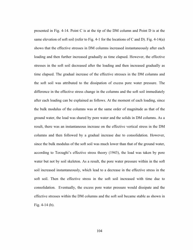
104

presented in Fig. 4-14. Point C is at the tip of the DM column and Point D is at the

same elevation of soft soil (refer to Fig. 4-1 for the locations of C and D). Fig. 4-14(a)

shows that the effective stresses in DM columns increased instantaneously after each

loading and then further increased gradually as time elapsed. However, the effective

stresses in the soft soil decreased after the loading and then increased gradually as

time elapsed. The gradual increase of the effective stresses in the DM columns and

the soft soil was attributed to the dissipation of excess pore water pressure. The

difference in the effective stress change in the columns and the soft soil immediately

after each loading can be explained as follows. At the moment of each loading, since

the bulk modulus of the columns was at the same order of magnitude as that of the

ground water, the load was shared by pore water and the solids in DM columns. As a

result, there was an instantaneous increase on the effective vertical stress in the DM

columns and then followed by a gradual increase due to consolidation. However,

since the bulk modulus of the soft soil was much lower than that of the ground water,

according to Terzaghi’s effective stress theory (1943), the load was taken by pore

water but not by soil skeleton. As a result, the pore water pressure within in the soft

soil increased instantaneously, which lead to a decrease in the effective stress in the

soft soil. Then the effective stress in the soft soil increased with time due to

consolidation. Eventually, the excess pore water pressure would dissipate and the

effective stresses within the DM columns and the soft soil became stable as shown in

Fig. 4-14 (b).

105

-40

0

40

80

120

160

0 2 4 6

Time (mon)

Add

ition

al v

ertic

al

effe

ctiv

e st

ress

(kPa

) Point CPoint D

(a) 1 month after service

0

50

100

150

200

250

0 100 200 300 400Time (mon)

Add

ition

al v

ertic

al

effe

ctiv

e st

ress

(kPa

)

Point CPoint D

(b) 30 years after service

Fig. 4-14. Additional Vertical Effective Stress versus Time of the 2D Baseline Case

106

Stress Concentration Ratio

Stress concentration ratio, n, is an important index to evaluate the efficiency of load

transfer between columns and soft soil. Stress concentration ratio is defined as the

ratio of the average vertical stress over columns to the average vertical stress over soft

soil and can be calculated as follows:

s

crcln

σ

σσ )(21

+= (4-3)

The notation is schematically shown in Fig. 4-15.

σs

σcl σcr

DM columnDM column Soft soil

σs

σcl σcr

DM columnDM column Soft soil

Fig. 4-15. Stress Concentration Ratio Calculation Illustration

107

Since the embankment and traffic loads are shared by the soft soil and the columns,

the additional vertical effective stresses were used in calculating the stress

concentration ratio. The stress concentration ratio profiles for the baseline case are

presented in Fig. 4-16, which shows that the stress concentration ratio decreased as

being away from the centerline. The maximum stress concentration ratio was 16.3 at

the span closest to the centerline of the embankment. The stress concentration ratio

increased slightly from 1 month to 30 years after service.

0

2

4

6

8

10

12

14

16

18

0 5 10 15 20Distance from the toe (m)

Stre

ss c

once

ntra

tion

ratio 1 month after service

30 years after service

Fig. 4-16. Stress Concentration Ratio Profiles of the 2D Baseline Case

108

Pore Water Pressure

The pore water pressure contours after partial dissipation are presented in Fig. 4-17.

The unit of the pore water pressure in the figure is Pascal (Pa). The excess pore water

pressures at four different locations with time up to 1 month after service and up to 30

years after service are presented in Fig. 4-18 and 4-19, respectively. The locations of

these points can be found in Fig. 4-1. Since Point D and C are located at the same

elevation, the excess pore water pressure are almost the same at those two points as

shown in Fig. 4-18. The excess pore water pressure at point D is higher than that at

Point E at 1 month after service, since Point D is further from the ground surface

(drainage surface) than Point E. However, at 30 years after service, the excess pore

water pressure at those two points almost dissipates completely as shown in Fig. 4-19.

Fig. 4-17. Pore Water Pressure Contour of the 2D Baseline Case

109

0

10

20

30

40

50

60

0 2 4 6Time (mon)

Exce

ss p

ore

wat

er

pres

sure

(kPa

)Point CPoint D

(a) 1 month after service

0

10

20

30

40

50

60

0 100 200 300 400

Time (mon)

Exce

ss p

ore

wat

er

pres

sure

(kPa

)

Point CPoint D

(b) 30 years after service

Fig. 4-18. Excess Pore Water Pressure at Point C and D versus Time of the 2D Baseline Case

110

0

10

20

30

40

50

60

0 2 4 6Time (mon)

Exce

ss p

ore

wat

er

pres

sure

(kPa

)

Point DPoint E

(a) 1 month after service

0

10

20

30

40

50

60

0 100 200 300 400Time (mon)

Exce

ss p

ore

wat

er

pres

sure

(kPa

)

Point DPoint E

(b) 30 years after service

Fig. 4-19. Excess Pore Water Pressure at Point D and E versus Time of the 2D Baseline Case

Fig. 4-20 presents the excess pore water pressure distribution along section I-I (refer

to Fig. 4-1). At the moment the embankment load was applied, since the bulk

modulus of the soft soil was much lower than that of water, the load was mainly

111

carried by water, which is attributed to the generation of excess pore water pressure.

As the time elapsed, the excess pore water pressure within the soft soil dissipated in

two ways: hydraulically and mechanically (Han and Ye 2001). Hydraulically, portion

of the excess pore water pressure dissipated by drainage and the corresponding load

was transferred to soil skeleton, which lead to the increase of the effective stress. On

the other hand, mechanically, as the effective stress in the soil increased, the soil

tended to settle more than the columns. As a result, portion of the load taken by pore

water would be transferred to the columns with the aid of shear stresses induced by

relative movement between the soft soil and the columns. This phenomenon was

discussed by Han and Ye (2001) when they studied the consolidation of the soft soil

treated by stone columns. In other words, the consolidation process in the GRCS

embankment system can not be evaluated by Terzaghi’s consolidation theory alone.

0

2

4

6

8

10

12

0 10 20 30 40 50 60Excess pore water pressure (kPa)

Dep

th (m

)

Stage 1Stage 2Stage 3Stage 4Stage 51 month after service30 years after service

Fig. 4-20. Excess Pore Water Pressure versus Depth of the 2D Baseline Case

112

The excess pore water pressure and the effective stress with time at Point D (refer to

Fig. 4-1) is shown in Fig. 4-21. Eventually, the excess pore water pressure dissipated

and the effective stress reached a constant value.

-30

0

30

60

90

0 2 4 6

Time (mon)

Exce

ss p

ore

wat

er

pres

sure

or a

dditi

onal

ef

fect

ive

verti

cal s

tress

(k

Pa)

Excess pore water pressureEffective vertical stress

(a) 1 month after service

0

20

40

60

0 100 200 300 400Time (mon)

Exce

ss p

ore

wat

er

pres

sure

or a

dditi

onal

ve

rtica

l effe

ctiv

e st

ress

(k

Pa)

Excess pore water pressureEffective vertical stress

(b) 30 years after service

Fig. 4-21. Excess Pore Water Pressure or Additional Vertical Effective Stress versus Time of the 2D Baseline Case

113

4.2 2D Parametric Study

4.2.1 Outline of 2D Parametric Study

Upon completion of the baseline case, a parametric study was performed by deviating

one property from the baseline case one at one time to investigate the influence of

that specific factor. The investigated factors are listed in Table 4-4. The elastic

modulus and friction angle of the embankment fill are controlled by the selection of

material and quality of compaction. The variations of those two parameters are not

significant in the practice. Consequently, these two parameters are not subjected to

change in this parametric study.

Table 4-4. Parameter and Variation Used in the Two-Dimensional Study

Item Parameter Range of value Elastic modulus (MPa) 1.0, 2.0*, 4.0, 8.0 Friction angle (o) 15, 20, 25*, 30 Soft soil Permeability (m/s) 10-8, 10-9*, 10-10 Elastic modulus (MPa) 100*, 150, 200 DM column Spacing (m) 2.0, 2.5*, 3.0

Geosynthetic Tensile stiffness (kN/m) 0, 1000*, 5000, 10000Construction Average construction rate (meter/mon) 0.25, 1*, 4

* parameters used in the baseline case

The soft soil modulus usually ranges from 1MPa to 15MPa (Budhu 2000). However,

the GRCS embankment system has been rarely used for soft soil with an elastic

114

modulus equal to 8MPa or higher. Therefore, the selected elastic moduli of the soft

soil were 1MPa, 2MPa, 4 MP, and 8MPa. Since the friction angle of the soft soil

typically ranges from 15o to 30o (Budhu 2000), the following friction angles were

selected in this study: 15o, 20o, 25o, and 30o. The permeability of a homogeneous clay

is usually less than 10-8m/s (Das 2001), therefore. The selected permeability values of

the soft soil were 10-8m/s, 10-9m/s, and 10-10m/s.

Three elastic moduli of DM columns were included in this parametric study:

100MPa, 150MPa, and 200MPa, which fall into the typical range of soil-cement

moduli (EPRI 1990). Based on constructed GRCS embankments, Han (1999) found

that the area replacement ratio of columns, defined as the ratio of column area to the

area of the embankment footprint, ranged from about 10% to about 22%. Therefore,

three DM column spacing were adopted in this study: 3m, 2.5m, and 2m, which are

equivalent to the area replacement ratio of 11%, 16%, and 25%, respectively.

The tensile stiffness of geosynthetics used in this study ranges from 0 to 10,000kN/m.

The 0kN/m tensile stiffness represents an unreinforced condition, while 10,000kN/m

is almost the highest tensile stiffness of geosynthetics in the current market. A tensile

stiffness of 1,000kN/m has been commonly used for geosynthetic reinforcement.

The construction rate of the baseline case was at 1meter/mon, which is commonly

used in the practice. In this parametric study, the construction rate was reduced to

115

one-forth and increased by four times to yield 0.25meter/mon and 4meter/mon,

respectively. The rates of 4meter/mon and 0.25meter/mon represent the fast

construction and the prolonged construction, respectively.

Many data can be extracted from all the numerical runs. It is impossible to present all

the numerical results in this dissertation; therefore, selected numerical results will be

presented and discussed, which are mainly focused on settlement, tension in

geosynthetic reinforcement, vertical stress, and excess pore water pressure.

4.2.2 Settlement

As usual, settlement is one of the focuses when the GRCS embankment is designed to

support roadways, railways, etc. In the past, however, most investigations have paid

attention to the settlement at the base of the embankment since the maximum long-

term settlement typically develops at this elevation. As illustrated in the analysis of

the baseline case, the post-construction settlement on the crest is actually more

critical to the serviceability of the structures on the embankment. Therefore, in this

study, more attention is paid to the settlement on the crest changing with time.

116

Influence of Soft Soil Elastic Modulus

Soft soil is characterized as high compressibility and low modulus. The influence of

the soft soil modulus was investigated by varying its value used in baseline case. The

settlement profiles on the crest and at the base of the embankment are presented at

different elastic moduli of soft soil in Fig. 4-22 and 4-23. It can be seen that the

increase of the soft soil modulus reduced the total and differential settlements both on

the crest and at the base. This phenomenon is more clearly presented in Fig. 4-24 and

4-25 for the maximum total and differential settlements on the crest and at the base of

the embankment. The degree of settlement reduction gradually decreased as the soft

soil modulus increased as indicated by the decrease of the curves’ slopes in Fig. 4-24

and 4-25. From 1 month to 30 years after service, both the maximum total settlement

and the maximum differential settlement increased due to the consolidation of soft

soil. However, the increase of the maximum settlement was much greater than that of

the maximum differential settlement.

117

05

1015202530354045

10 12 14 16 18 20

Distance from the toe (m)

Settl

emen

t (m

m)

1 2 4 8Es (MPa)

(a) On the crest

0

10

20

30

40

50

60

70

0 5 10 15 20

Distance from the toe (m)

Settl

emen

t (m

m)

1 2 4 8Es (MPa)

(b) At the base

Fig. 4-22. Settlement Profiles for Various Soil Moduli at 1 Month after Service (2D)

118

0

510

1520

2530

3540

45

10 12 14 16 18 20

Distance from the toe (m)

Settl

emen

t (m

m)

1 2 4 8Es (MPa)

(a) On the crest

0

10

20

30

40

50

60

70

0 5 10 15 20Distance from the toe (m)

Settl

emen

t (m

m)

1 2 4 8Es (MPa)

(b) At the base

Fig. 4-23. Settlement Profiles for Various Soil Moduli at 30 Years after Service (2D)

119

0

10

20

30

40

50

60

70

1 2 3 4 5 6 7 8Soil modulus (MPa)

Max

imum

set

tlem

ent (

mm

)

1 month after service (crest)30 years after service (crest)1 month after service (base)30 years after service (base)

Fig. 4-24. Maximum Settlement versus Soil Modulus (2D)

0

10

20

30

40

1 2 3 4 5 6 7 8Soil modulus (MPa)

Max

imum

diff

eren

tial s

ettle

men

t(m

m)

1 month after service (crest)30 years after service (crest)1 month after sevice (base)30 years after service (base)

Fig. 4-25. Maximum Differential Settlement versus Soil Modulus (2D)

120

Since the differential settlements at the crest are crucial to the serviceability, they are

evaluated using the distortion concept defined in the earlier section in the baseline

case. Fig. 4-26 presents the influence of the soft soil modulus on the maximum

distortion. Obviously, the increase of soft soil modulus reduced the maximum

distortion and the consolidation had limited influence on the distortion at various soft

soil moduli.

0

0.1

0.2

0.3

0.4

0.5

1 3 5 7Soil modulus (MPa)

Max

imum

dis

torti

on (%

)

1 month after service30 years after service

Fig. 4-26. Maximum Distortion on the Crest versus Soil Modulus (2D)

Influence of Soft Soil Friction Angle

Effective friction angle (φ′) is a strength parameter and should not influence the

settlement as long as the soil remains elastic. However, local yielding or failure is

121

almost inevitable in this system; therefore, the friction angle is expected to have some

influence on the settlement of the GRCS embankment system. The influence of the

friction angle is investigated by changing the soft soil effective friction angle from the

baseline case. The settlement profiles at 1 month and 30 years after service are

presented in Fig. 4-27 and 4-28, respectively. Generally speaking, the increase of the

friction angle led to a decrease in the settlement. This phenomenon is also

demonstrated in Fig. 4-29 and 4-30.

When the soft soil friction angle ranged from 20o to 30o, their settlements were close.

However, the settlements at the friction angle of 15o were much larger than those with

higher friction angles. This difference resulted from the fact that a greater extent of

yielding or failure occurred at the friction angle of 15o. In addition, the soil friction

angle had much less effect on the settlements on the crest than those at the base. In

Fig. 4-29, the curve of the maximum settlement on the crest is almost flat after the

friction angle is higher than 20o. Therefore, it may be concluded that the influence of

the friction angle on the settlement on the crest is insignificant as long as no

considerable failure develops in the soft soil.

122

10

15

20

25

30

35

40

10 12 14 16 18 20

Distance from the toe (m)

Settl

emen

t (m

m) 15 20 25 30

φ (o)

(a) On the crest

0

10

20

30

40

50

60

0 5 10 15 20Distance from the toe (m)

Settl

emen

t (m

m)

15 20 25 30φ (o)

(b) At the base

Fig. 4-27. Settlement Profiles for Various Friction Angles at 1 Month after Service (2D)

123

10

15

20

25

30

35

40

10 12 14 16 18 20Distance from the toe (m)

Settl

emen

t (m

m)

15 20 25 30φ (o)

(a) On the crest

0

10

20

30

40

50

60

70

0 5 10 15 20

Distance from the toe (m)

Settl

emen

t (m

m) 15 20 25 30

φ (o)

(b) At the base

Fig. 4-28. Settlement Profiles for Various Friction Angles at 30 Years after Service (2D)

124

0

10

20

30

40

50

60

70

15 20 25 30Friction angle (o)

Max

imum

set

tlem

ent (

mm

) 1 month after service (crest)30 years after service (crest)1 month after service (base)30 years after service (base)

Fig. 4-29. Maximum Settlement versus Friction Angle (2D)

0

5

10

15

20

25

30

35

15 20 25 30Friction angle (o)

Max

imum

diff

eren

tial s

ettle

men

t (m

m)

1 month after service (crest)30 years after service (crest)1 month after service (base)30 years after service (base)

Fig. 4-30. Maximum Differential Settlement versus Friction Angle (2D)

125

Similarly, the influence of the friction angle on the maximum distortion was

evaluated and is shown in Fig. 4-31. It can be found that the variation of the distortion

with respect to the friction angle was limited.

0

0.1

0.2

0.3

0.4

0.5

15 20 25 30Friction angle (o)

Max

imum

dis

torti

on (%

)

1 month after service30 years after service

Fig. 4-31. Maximum Distortion on the Crest versus Friction Angle (2D)

Influence of Soft Soil Permeability

The permeability of the soft soil is expected to greatly influence the generation and

dissipation of the excess pore water pressure; therefore, it should have a profound

influence on the post-construction settlements on the crest as well, which have not

been well studied in the past.

126

0

5

10

15

20

25

30

35

10 12 14 16 18 20Distance from the toe (m)

Settl

emen

t (m

m)

100 10 1k (x10-10m/s)

(a) On the crest

0

10

20

30

40

50

0 5 10 15 20Distance from the toe (m)

Settl

emen

t (m

m)

100 10 1k (x10-10m/s)

(b) At the base

Fig. 4-32. Settlement Profiles for Various Permeability at 1 Month after Service (2D)

127

05

1015

2025

3035

4045

10 12 14 16 18 20Distance from the toe (m)

Settl

emen

t (m

m)

100 10 1k (x10-10m/s)

(a) On the crest

0

10

20

30

40

50

60

70

0 5 10 15 20Distance from the toe (m)

Settl

emen

t (m

m)

100 10 1k (x10-10m/s)

(b) At the base

Fig. 4-33. Settlement Profiles for Various Permeability at 30 Years after Service (2D)

128

Figures 4-32 and 4-33 present the numerical results which show the higher

permeability of the soft soil having the lower settlements, both at the base and on the

crest. This finding is more clearly illustrated in Fig. 4-34 and Fig. 4-35, i.e., the

maximum settlement and the maximum differential settlement decreased with the

increase of the soil permeability.

0

10

20

30

40

50

60

70

0 20 40 60 80 100Soil permeability (x10-10m/s)

Max

imum

set

tlem

ent (

mm

)

1 month after service (crest)30 years after service (crest)1 month after service (base)30 years after service (base)

Fig. 4-34. Maximum Settlement versus Soil Permeability (2D)

In addition, the difference in the maximum settlement and the maximum differential

settlement at 1 month and 30 years after service decreased with the increase of the

soil permeability. In other words, the post-construction settlements can be minimized

by increasing the soil permeability. Figure 4-35 shows that the slopes of curves for

the differential settlements at 30 years after service were very steep when the soil

permeability was lower than 10-9m/s. This phenomenon implies that it is effective to

129

reduce the post-construction settlement by increasing the soil permeability while the

permeability is lower than 10-9m/s.

0

5

10

15

20

25

30

35

0 20 40 60 80 100Soil permeability (x10-10m/s)

Max

imum

diff

eren

tial s

ettle

men

t(m

m)

1 month after service (crest)30 years afer service (crest)1 month after service (base)30 years after service (base)

Fig. 4-35. Maximum Differential Settlement versus Soil Permeability (2D)

Another interesting finding from Fig. 4-32 (b) is that at 1 month after service, the soft

soil with lower permeability had larger settlement in the soft soil but smaller

settlement in the columns. This phenomenon is associated with fact that the lower the

soil permeability, the higher the excess pore water pressure in the soft soil. The higher

excess pore water pressure in the soft soil shared more load from the embankment.

Therefore, the lower permeability soil led to smaller settlements in the columns.

Meanwhile, the higher excess pore water pressure in the soft soil led to a greater

reduction in the effective stress in the soft soil. Since the soil strength is effective

130

stress dependant, the soil at the lower effective stress fails more easily. As a result,

the soil settled more when the permeability of the soft soil was lower. As the

consolidation proceeded, the load carried by pore water was transferred back to the

columns and/or the soft soil. The higher excess pore water pressure would have more

load transferred. Consequently, the lower permeability of the soft soil induced the

greater increase of the settlement from 1 month to 30 years after service.

The maximum distortion is plotted against the soil permeability in Fig. 4-36.

0

0.1

0.2

0.3

0.4

0.5

0 20 40 60 80 100Soil permeability (x10-10m/s)

Max

imum

dis

torti

on (%

)

1 month after service30 years after service

Fig. 4-36. Maximum Distortion on the Crest versus Soil Permeability (2D)

Apparently, the higher permeability yielded less distortion. As mentioned earlier,

part of the distortion on the crest was induced by the continued consolidation of the

131

soft soil after the construction. As the soil permeability was higher, the less excess

pore water pressure accumulated during the construction, which led to less distortion.

Figure 4-36 also shows that there was a great increase in the distortion from 1 month

to 30 years after service when the soil permeability was low. The finding implies that

it is necessary to consider the influence of the soil permeability on the serviceability

of the GRCS embankment, especially when the soil permeability is low.

Influence of Column Elastic Modulus

In this study, DM columns are investigated and their moduli can be correlated to their

undrained shear strengths using the generally accepted equation: Ec=200c, where c is

the cohesion of the columns. Therefore, the column modulus is not only an indicator

of stiffness but also an indicator of strength. It is expected that the stiffness of the

columns plays an important role in limiting the settlements. Stiffer columns are

expected to carry a larger portion of the embankment and traffic loads to reduce the

settlements because less load is taken by the soft soil. The effect of the elastic moduli

of the columns on the settlements is presented in Fig. 4-37 and 4-38.

132

0

5

10

15

20

25

30

10 12 14 16 18 20Distance from the toe (m)

Settl

emen

t (m

m) 100 150 200

Ec (MPa)

(a) On the crest

0

10

20

30

40

50

0 5 10 15 20Distance from the toe (m)

Settl

emen

t (m

m)

100 150 200Ec (MPa)

(b) At the base

Fig. 4-37. Settlement Profiles for Various Column Moduli at 1 Month after Service (2D)

133

0

5

10

15

20

25

30

35

10 12 14 16 18 20Distance from the toe (m)

Settl

emen

t (m

m)

100 150 200

Ec (MPa)

(a) On the crest

0

10

20

30

40

50

60

0 5 10 15 20Distance from the toe (m)

Settl

emen

t (m

m)

100 150 200

Ec (MPa)

(b) At the base

Fig. 4-38. Settlement Profiles for Various Column Moduli at 30 Years after Service (2D)

134

0

10

20

30

40

50

60

70

50 100 150 200Column modulus (MPa)

Max

imum

set

tlem

ent (

mm

)1 month after service (crest)30 years after service (crest)1 month after service (base)1 month after service (base)

Fig. 4-39. Maximum Settlement versus Column Modulus (2D)

0

5

10

15

20

25

100 120 140 160 180 200Column modulus (MPa)

Max

imum

diff

eren

tial s

ettle

men

t (m

m)

1 month after service (crest)30 years after service (crest)1 month after service (base)30 years after service (base)

Fig. 4-40. Maximum Differential Settlement versus Column Modulus (2D)

135

A comparison between Fig. 4-39 and 4-40 shows that the increase of the column

modulus had a greater effect on the reduction of the maximum settlement than that of

the maximum differential settlement. Figure 4-40 also shows that the curves of

maximum differential settlement on the crest against the column modulus are so flat

that the reduction in the maximum differential settlement was less than 2mm as the

column modulus increased from 100MPa to 200MPa. The major reason for this

phenomenon may be because the columns were stiff enough as compared with the

soft soil and the stable soil arching was formed. In this study, the modulus ratios of

column to soft soil ranged from 50 to 100. The high modulus ratio makes the column

behave as a rigid support with respect to the soft soil. As a result, beyond a certain

height of the embankment, the embankment settlements are almost uninfluenced by

the column modulus.

Due to its limited influence on the differential settlement, the column modulus also

had limited influence on the maximum distortion as shown in Fig. 4-41. Figure 4-41

shows that the maximum distortion increased slightly with consolidation.

136

0

0.1

0.2

0.3

0.4

0.5

100 120 140 160 180 200Column modulus (MPa)

Max

imum

dis

torti

on (%

)

1 month after service30 years after service

Fig. 4-41. Maximum Distortion on the Crest versus Column Modulus (2D)

Influence of Column Spacing

Column spacing is another important design parameter. Once the column size is

determined, the column spacing is directly related to the area replacement ratio of the

columns, i.e., larger spacing of columns leads to a smaller area replacement. Figures

4-42, 4-43, 4-44, and 4-45 show that larger spacing of columns resulted in larger total

and differential settlements at the base and on the crest of the embankment. The

increase of column spacing reduced the area replacement ratio so that the percentage

of the soft soil area increased but the percentage of the column area decreased. Since

the soft soil was much softer than the columns and it settled more than the columns,

the differential settlement between the columns and the soft soil increased. Figures 4-

137

42 and 4-43 also show that apparent local differential settlements developed at the

crest when the column spacing equaled to 3.0m. Figure 4-45 indicates that the

maximum differential settlement was more than doubled as the column spacing

increased from 2.0 to 3.0m. The comparison between Fig. 4-44 and 4-45 shows that

the time from 1 month to 30 years after service had more effect on the maximum

settlement than the maximum differential settlement.

05

1015202530354045

10 12 14 16 18 20

Distance from the toe (m)

Settl

emen

t (m

m)

2.0 2.5 3.0s (m)

(a) On the crest

Fig. 4-42. Settlement Profiles for Various Column Spacing at 1 Month after Service (2D)

138

0

10

20

30

40

50

60

0 5 10 15 20Distance from the toe (m)

Settl

emen

t (m

m)

2.0 2.5 3.0s (m)

(b) At the base

Fig. 4-42. Settlement Profiles for Various Column Spacing at 1 Month after Service (2D) (continued)

05

1015202530354045

10 12 14 16 18 20

Distance from the toe (m)

Settl

emen

t (m

m)

2.0 2.5 3.0s (m)

(a) On the crest

Fig. 4-43. Settlement Profiles for Various Column Spacing at 30 Years after Service (2D)

139

0

10

20

30

40

50

60

70

0 5 10 15 20Distance from the toe (m)

Settl

emen

t (m

)

2.0 2.5 3.0s (m)

(b) At the base

Fig. 4-43. Settlement Profiles for Various Column Spacing at 30 Years after Service (2D) (continued)

0

10

20

30

40

50

60

70

2 2.5 3Column spacing (m)

Max

imum

set

tlem

ent (

mm

) 1 month after service (crest)30 years after service (crest)1 month after service (base)30 years after service (base)

Fig. 4-44. Maximum Settlement versus Column Spacing (2D)

140

0

5

10

15

20

25

30

35

2 2.5 3Column spacing (m)

Max

imum

diff

eren

tial s

ettle

men

t (m

m)

1 month after service (crest)30 years after service (crest)1 month after service (base)30 years after service (base)

Fig. 4-45. Maximum Differential Settlement versus Column Spacing (2D)

0

0.1

0.2

0.3

0.4

0.5

2 2.5 3Column spacing (m)

Max

imum

dis

torti

on (%

)

1 month after service30 years after service

Fig. 4-46. Maximum Distortion on the Crest versus Column Spacing (2D)

141

The maximum distortion is plotted against the column spacing in Fig. 4-46 to

investigate the influence of the column spacing on the distortion. It is shown that the

column spacing had a noticeable influence on the distortion and the larger column

spacing had the greater distortion.

Influence of Geosynthetic Tensile Stiffness

Geosynthetic tensile stiffness, J, is an important material property of geosynthetics.

Depending on the type of geosynthetic used, the tensile stiffness can vary greatly. In

this study, the tensile stiffness varied from zero to 10,000kN/m. Zero tensile stiffness

represents a case without reinforcement, while 10,000kN/m is almost the highest

tensile stiffness of geosynthetics available in the current market.

Figures 4-47 and 4-48 present the settlement profiles at the base and on the crest of

the embankment using one layer geosynthetic at different tensile stiffness. Clearly,

the influence of the geosynthetic tensile stiffness on the settlement was limited.

Especially for the geosynthetic at the tensile stiffness from 1,000 to 10,000kN/m, the

reduction in the settlement on the crest was almost negligible. This finding is more

clearly demonstrated in Figs. 4-49 and 4-50. Even though the geosynthetic tensile

stiffness had some impact on the settlement at the base, its influence on the settlement

at the crest was much less.

142

0

5

10

15

20

25

30

10 12 14 16 18 20

Distance from the toe (m)

Settl

emen

t (m

m) 0 1000 5000 10000

J (kN/m)

(a) On the crest

0

10

20

30

40

50

0 5 10 15 20

Distance from the toe (m)

Settl

emen

t (m

m)

0 1000 5000 10000J (kN/m)

(b) At the base

Fig. 4-47. Settlement Profiles for Various Tensile Stiffness at 1 Month after Service (2D)

143

0

5

10

15

20

25

30

35

10 12 14 16 18 20

Distance from the toe (m)

Settl

emen

t (m

m)

0 1000 5000 10000J (kN/m)

(a) On the crest

0

10

20

30

40

50

60

0 5 10 15 20

Distance from the toe (m)

Settl

emen

t (m

m)

0 1000 5000 10000J (kN/m)

(b) At the base

Fig. 4-48. Settlement Profiles for Various Tensile Stiffness at 30 Years after Service (2D)

144

0

10

20

30

40

50

60

0 2000 4000 6000 8000 10000

Tensile stiffness (kN/m)

Max

imum

set

tlem

ent (

mm

) 1 month after service (crest)30 years after service (crest)1 month after service (base)30 years after service (base)

Fig. 4-49. Maximum Settlement versus Tensile Stiffness (2D)

0

5

10

15

20

25

0 2000 4000 6000 8000 10000Tensile stiffness (kN/m)

Max

imum

diff

eren

tial s

ettle

men

t (m

m)

1 month after service (crest)30 years after service (crest)1 month after service (base)30 years after service (base)

Fig. 4-50. Maximum Differential Settlement versus Tensile Stiffness (2D)

145

Similar to its negligible influence on the differential settlement, the geosynthetic

tensile stiffness also exhibited negligible influence on the distortion as shown in Fig.

4-51.

0

0.1

0.2

0.3

0.4

0.5

0 2000 4000 6000 8000 10000Tensile stiffness (kN/m)

Max

imum

dis

torti

on (%

)

1 month after service30 years after service

Fig. 4-51. Maximum Distortion on the Crest versus Tensile Stiffness (2D)

Influence of Construction Rate

In addition to soil properties (elastic modulus, friction angle, and permeability) and

column dimensions and properties (spacing and elastic modulus), the rate of

construction can have profound influence on the performance of the GRCS

embankments. In this study, one of the most important construction parameters, the

average construction rate, was investigated. The average construction rate here was

146

defined as the thickness of the lift built in unit time. As discussed earlier in the

baseline case, the embankment was built into five stages of equal thickness, i.e., 1m

at each stage. The duration of each stage was one month. Therefore, the average

construction rate for the baseline case was 1meter/mon, which is the rate commonly

used in practice. In this study, the average construction rate of the baseline case

decreased to one-fourth (i.e., 0.25meter/mon) and increased to 4 times (i.e.,

4meter/mon) to represent the prolonged construction and the fast construction,

respectively.

The influence of the average construction rate on the settlements is shown in Fig. 4-

52, 4-53, 4-54, and 4-55, which show that the higher construction rate induced greater

settlement. As compared with the effect of soil permeability, the lower average

construction rate had the effect on the accumulated less excess pore water pressure,

which is similar to the effect of the higher permeability of the soil as discussed in the

permeability section. Figure 4-52 also shows that the settlements of columns were

smaller but the settlements of the soft soil were larger at a higher average construction

rate. The same explanation can be offered as that stated in the permeability section.

147

0

5

10

15

20

25

30

35

10 12 14 16 18 20Distance from the toe (m)

Settl

emen

t (m

m) 4 1 0.25

v (meter/mon)

(a) On the crest

0

10

20

30

40

50

60

0 5 10 15 20Distance from the toe (m)

Settl

emen

t (m

m)

4 1 0.25v (meter/mon)

(b) At the base

Fig. 4-52. Settlement Profiles for Various Average Construction Rates at 1 Month after Service (2D)

148

0

5

10

15

2025

30

35

40

45

10 12 14 16 18 20Distance from the toe (m)

Settl

emen

t (m

m)

4 1 0.25

v (meter/mon)

(a) On the crest

0

10

20

30

40

50

60

0 5 10 15 20Distance from the toe (m)

Settl

emen

t (m

m)

4 1 0.25

v (meter/mon)

(b) At the base

Fig. 4-53. Settlement Profiles for Various Average Construction Rates at 30 Years after Service (2D)

149

0

10

20

30

40

50

60

0 1 2 3 4Average construction rate (meter/mon)

Max

imum

set

tlem

ent (

mm

) 1 month after service (crest)30 years after service (crest)1 month after service (base)30 years after service (base)

Fig. 4-54. Maximum Settlement versus Average Construction Rate (2D)

0

5

10

15

20

25

30

0 1 2 3 4Average construction rate (meter/mon)

Max

imum

diff

eren

tial s

ettle

men

t (m

m)

1 month after service (crest)30 years after service (crest)1 month after service (base)30 years after service (base)

Fig. 4-55. Maximum Differential Settlement versus Average Construction Rate (2D)

150

The influence of the average construction rate on the maximum distortion is presented

in Fig. 4-56. The lower average construction rate yielded the smaller maximum

distortion.

0

0.1

0.2

0.3

0.4

0.5

0 1 2 3 4Average construction rate (meter/mon)

Max

imum

dis

torti

on (%

)

1 month after service30 years after service

Fig. 4-56. Maximum Distortion on the Crest versus Average Construction Rate (2D)

4.2.3 Tension Developed in Geosynthetics

In the GRCS embankment, geosynthetic reinforcement plays dual functions.

Primarily, it works a flexible layer bridging over soft soil to transfer load from the

soft soil to the columns. This function has been widely accepted and considered in the

151

design. Secondarily, it can counteract lateral spreading of the embankment fill.

Hence, the tension developed in the geosynthetic reinforcement is the resultant of the

tension induced by these two effects.

Tension in geosynthetic reinforcement is one of the focuses in research and design. In

a few GRCS embankment projects, the tension in the geosynthetic reinforcement was

monitored by strain gauges. The level of tension developed in geosynthetic

reinforcement may have some influence on its creep behavior, which needs to be

accounted for in some applications. However, the creep behavior is beyond the scope

of this study. In this study, the geosynthetic was assumed to have constant tensile

stiffness and cross section. The influences of the soft soil modulus, the soil friction

angle, the soil permeability, the column modulus, the column spacing, the tensile

stiffness of geosynthetic, and the average construction rate on the tension in the

geosynthetic reinforcement were investigated.

Influence of Soft Soil Elastic Modulus

In the 2D parametric study, the geosynthetic sheet was modeled as lineal cable

elements and only the tension developed in the direction perpendicular to traffic

direction was available. The tension profiles at different soft soil moduli are presented

in Fig. 4-57 and the maximum tension against soft soil modulus is presented in Fig. 4-

58. Obviously, the higher soft soil modulus yielded the lower tension in the

152

geosynthetic sheet. As discussed in the settlement section, smaller differential

settlement occurred at a higher soft soil modulus, as a consequence, the geosynthetic

sheet was less stretched and lower tension was generated. Figure 4-57 shows that

higher tension in the geosynthetic reinforcement developed over columns, which is

consistent with the finding by Han and Gabr (2002). It is also shown that the

maximum tension developed at a certain distance from the centerline of the

embankment, which is consistent with the location of the maximum settlement at the

base of the embankment. In addition, the tension was almost unchanged from one

month to 30 years after service. This phenomenon implies that the post-construction

consolidation had a limited effect on the tension in the geosynthetic reinforcement.

0

2

4

6

8

10

12

0 5 10 15 20Distance from the toe (mm)

Tens

ion

(kN

/m)

1 2 4 8Es (MPa)

(a) 1 month after service

Fig. 4-57. Tension Profiles for Various Soil Moduli at 1 Month and 30 Years after Service (2D)

153

0

2

4

6

8

10

12

0 5 10 15 20

Distance from the toe (m)

Tens

ion

(kN

/m)

1 2 4 8Es (MPa)

(b) 30 years after service

Fig. 4-57. Tension Profiles for Various Soil Moduli at 1 Month and 30 Years after Service (2D) (continued)

0

2

4

6

8

10

12

1 2 3 4 5 6 7 8Soil modulus (MPa)

Max

imum

tens

ion

(kN

/m) 1 month after service

30 years after service

Fig. 4-58. Maximum Tension versus Soil Modulus (2D)

154

Influence of Soft Soil Friction Angle

The tension profiles at different soil friction angles are presented in Fig 4-59. It is

shown that the tension developed at the soil friction angle from 20o to 30o was close.

However, the tension developed at the soil friction angle of 15o was much higher than

that at the other soil friction angles from 20o to 30o. This trend can be seen more

clearly in Fig. 4-60. This finding is consistent with the development of settlement as

discussed earlier, i.e., as long as the soil remained in an elastic state, the soil friction

angle would not have much influence on the tension.

0

2

4

6

8

10

12

0 5 10 15 20

Distance from the toe (m)

Tens

ion

(kN

/m)

15 20 25 30φ (o)

(a) 1 month after service

Fig. 4-59. Tension Profiles for Various Friction Angles at 1 Month and 30 Years after Service (2D)

155

0

2

4

6

8

10

12

0 5 10 15 20

Distance from the toe (m)

Tens

ion

(kN

/m)

15 20 25 30φ (o)

(b) 30 years after service

Fig. 4-59. Tension Profiles for Various Friction Angles at 1 Month and 30 Years after Service (2D) (continued)

0

2

4

6

8

10

12

15 20 25 30

Friction angle (o)

Max

imum

tens

ion

(kN

/m)

1 month after service30 years after service

Fig. 4-60. Maximum Tension versus Friction Angle (2D)

156

Influence of Soft Soil Permeability

Related to the lower soil permeability leading to the larger differential settlement at

the base, the lower soil permeability also induced the higher tension in the

geosynthetic reinforcement as shown in Fig. 4-61 and 4-62. There was a noticeable

increase in the maximum tension from one month to 30 years after service at the soil

permeability lower or equal to 10-10m/s. However, this difference became

insignificant when the soil permeability was higher than 10-10m/s. This finding is

consistent with the result of the differential settlement from one month to 30 years

after service.

0

2

4

6

8

10

0 5 10 15 20Distance from the toe (m)

Tens

ion

(kN

/m)

100 10 1k (x10-10m/s)

(a) 1 month after service

Fig. 4-61. Tension Profiles for Various Soil Permeability at 1 Month and 30 Years after Service (2D)

157

0

2

4

6

8

10

12

0 5 10 15 20

Distance from the toe (m)

Tens

ion

(kN

/m)

100 10 1k (x10-10m/s)

(b) 30 years after service

Fig. 4-61. Tension Profiles for Various Soil Permeability at 1 Month and 30 Years after Service (2D) (continued)

0

2

4

6

8

10

12

0 20 40 60 80 100Soil permeability (x10-10m/s)

Max

imum

tens

ion

(kN

/m) 1 month after service

30 years after service

Fig. 4-62. Maximum Tension versus Soil Permeability (2D)

158

Influence of Column Elastic Modulus

Similar to the influence on the differential settlement at the base, the column modulus

had a very limited influence on the tension in the geosynthetic reinforcement.

Compared with the soft soil, the columns in this study were rigid enough to help the

development of stable soil arching. As a consequence, the increase of column

modulus did not considerably reduce the load carried by the geosynthetic

reinforcement. Consolidation of the soft soil did not have any significant influence on

the maximum tension either as shown in Fig. 4-64.

0

2

4

6

8

0 5 10 15 20

Distance from the toe (m)

Tens

ion

(kN

/m) 100 150 200

Ec (MPa)

(a) 1 month after service

Fig. 4-63. Tension Profiles for Various Column Moduli at 1 Month and 30 Years after Service (2D)

159

0

2

4

6

8

0 5 10 15 20Distance from the toe (m)

Tens

ion

(kN

/m)

100 150 200Ec (MPa)

(b) 30 years after service

Fig. 4-63. Tension Profiles for Various Column Moduli at 1 Month and 30 Years after Service (2D) (continued)

0

2

4

6

8

10

12

100 150 200Column modulus (MPa)

Max

imum

tens

ion

(kN

/m)

1 month after service30 years after service

Fig. 4-64. Maximum Tension versus Column Modulus (2D)

160

Influence of Column Spacing

As discussed earlier, the column spacing at a fixed column size is directly related to

the area replacement ratio. Figures 4-65 and 4-66 present the tension profiles at

different column spacing. Due to the difference in the column spacing, the maximum

tension did not occur at the same location. However, it was located over a column and

at a certain distance from the centerline. Figure 4-66 shows that the larger spacing

yielded the higher maximum tension. In addition, the consolidation had a limited

influence on the maximum tension within the range of the column spacing

investigated.

0

2

4

6

8

10

12

0 5 10 15 20Distance from the toe (m)

Tens

ion

(kN

/m)

2.0 2.5 3.0

s (m)

(a) 1 month after service

Fig. 4-65. Tension Profiles for Various Column Spacing at 1 Month and 30 Years after Service (2D)

161

0

2

4

6

8

10

12

0 5 10 15 20

Distance from the toe (m)

Tens

ion

(kN

/m)

2.0 2.5 3.0

s (m)

(b) 30 years after service

Fig. 4-65. Tension Profiles for Various Column Spacing at 1 Month and 30 Years after Service (2D) (continued)

0

2

4

6

8

10

12

2 2.5 3

Column spacing (m)

Max

imum

tens

ion

(kN

/m) 1 month after service

30 years after service

Fig. 4-66. Maximum Tension versus Column Spacing (2D)

162

Influence of Geosynthetic Tensile Stiffness

Unlike the influence on the settlements, the geosynthetic tensile stiffness had a

significant influence on the tension as shown in Fig. 4-68. The maximum tension

almost increased linearly when the tensile stiffness increased from 1,000 to

10,000kN/m. It is known that the tension is equal to the product of the tensile

stiffness and the strain. Under various tensile stiffness levels, the differential

settlement at the base was almost unchanged, which led to the unchanged strain. As a

result, the product of the tensile stiffness and the strain increased almost linearly.

0

10

20

30

40

50

0 5 10 15 20

Distance from the toe (m)

Tens

ion

(kN

/m)

1000 5000 10000J (kN/m)

(a) 1 month after service

Fig. 4-67. Tension Profiles for Various Tensile Stiffness at 1 Month and 30 Years after Service (2D)

163

0

10

20

30

40

50

0 5 10 15 20

Distance from the toe (m)

Tens

ion

(kN

/m)

1000 5000 10000J (kN/m)

(b) 30 years after service

Fig. 4-67. Tension Profiles for Various Tensile Stiffness at 1 Month and 30 Years after Service (2D) (continued)

0

10

20

30

40

50

0 2000 4000 6000 8000 10000

Tensile stiffness (kN/m)

Max

imum

tens

ion

(kN

/m) 1 month after service

30 years after service

Fig. 4-68. Maximum Tension versus Tensile Stiffness (2D)

164

Influence of Construction Rate

Figures 4-69 and 4-70 present the tension profiles at different construction rates. As

discussed in the settlement section, the higher construction rate led to the larger

differential settlement, especially at the base of the embankment, which induced the

higher tension.

0

2

4

6

8

10

0 5 10 15 20

Distance from the toe (m)

Tens

ion

(kN

/m)

4 1 0.25

v (meter/mon)

(a) 1 month after service

Fig. 4-69. Tension Profiles for Various Average Construction Rates at 1 Month and 30 Years after Service (2D)

165

0

2

4

6

8

10

0 5 10 15 20

Distance from the toe (m)

Tens

ion

(kN

/m)

4 1 0.25

v (meter/mon)

(b) 30 years after service

Fig. 4-69. Tension Profiles for Various Average Construction Rates at 1 Month and 30 Years after Service (2D) (continued)

0

2

4

6

8

10

12

0 1 2 3 4Average construction rate (meter/mon)

Max

imum

tens

ion

(kN

/m)

1 month after service30 years after service

Fig. 4-70. Maximum Tension versus Average Construction Rate (2D)

166

4.2.4 Vertical Stress and Stress Concentration Ratio

One of the key mechanisms of the GRCS embankment is to transfer the load from the

soft soil to the columns through soil arching. As the load is transferred from the soft

soil to the columns, higher vertical stresses develop in the columns than in the soft

soil. As discussed in the baseline section of this chapter, the stress concentration ratio,

n, is commonly used to evaluate the load transfer efficiency. The stress concentration

ratio is defined as the average vertical stress on the column heads to the average

vertical stress in the soft soil at the same elevation.

Similar to the approach used in the baseline case, the additional vertical effective

stress at the base of the embankment due to the embankment and traffic load was

used to calculate the stress concentration ratio. The influence of various factors on the

stress concentration ratio is presented below.

Influence of Soft Soil Elastic Modulus

The additional vertical effective stress profiles at the elevation of the column heads

are presented with the different soft soil moduli in Fig. 4-71.

167

0

100

200

300

400

0 5 10 15 20

Distance from the toe (m)

Add

ition

al v

ertic

al e

ffect

ive

stre

ss

(kPa

)

1 2 4 8Es (MPa)

(a) 1 month after service

0

100

200

300

400

0 5 10 15 20Distance from the toe (m)

Add

ition

al v

ertic

al e

ffect

ive

stre

ss

(kPa

)

1 2 4 8Es (MPa)

(b) 30 years after service

Fig. 4-71. Additional Vertical Effective Stress Profiles for Various Soil Moduli (2D)

168

It was indicated in Fig. 4-71 that the increase of the soft soil modulus reduced the

additional vertical effective stress on the column heads but increased that on the soft

soil. This result can be explained that the increase of the soft soil modulus reduced the

stiffness difference between the soft soil and the columns; consequently, the soft soil

shared more load with the columns. Figure 4-71 shows that the additional effective

stresses slightly increased both over the columns and over the soft soil from 1 month

to 30 years after service due to the dissipation of excess pore water pressure.

The stress concentration ratio profiles are presented in Fig. 4-72. It can be seen that

the higher stress concentration ratio was close to the centerline. In addition, the higher

soft soil modulus yielded the lower stress concentration ratio. The profiles of the

stress concentration ratios at one month or 30 years after service show that

consolidation had a slight influence on the stress concentration ratio.

169

0

5

10

15

20

25

30

35

0 5 10 15 20Distance from the toe (m)

Stre

ss c

once

ntra

tion

ratio 1 2 4 8

Es (MPa)

(a) 1 month after service

0

5

10

15

20

25

30

35

0 5 10 15 20Distance from the toe (m)

Stre

ss c

once

ntra

tion

ratio 1 2 4 8

Es (MPa)

(b) 30 years after service

Fig. 4-72. Stress Concentration Ratio Profiles for Various Soil Moduli (2D)

170

Influence of Soft Soil Friction Angle

The profiles of the additional vertical effective stresses at various soil friction angles

are presented in Fig. 4-73, which shows that a higher soil friction angle led to slightly

higher additional vertical effective stresses in the soft soil and slightly lower

additional vertical effective stresses in the columns. The phenomenon was attributed

to the reduction in the differential settlement at the base with the increase of the soil

friction angle. In addition, the consolidation of the soft soil did not have much

influence on the additional vertical effective stress.

0

100

200

300

400

0 5 10 15 20Distance from the toe (m)

Add

ition

al v

ertic

al e

ffect

ive

stre

ss

(kPa

)

15 20 25 30φ (o)

(a) 1 month after service

Fig. 4-73. Additional Effective Stress Profiles for Various Friction Angles (2D)

171

0

100

200

300

400

0 5 10 15 20

Distance from the toe (m)

Add

ition

al v

ertic

al e

ffect

ive

stre

ss (k

Pa)

15 20 25 30φ (o)

(b) 30 years after service

Fig. 4-73. Additional Effective Stress Profiles for Various Friction Angles (2D) (continued)

The profiles of the stress concentration ratio at different soil friction angles are

presented in Fig. 4-74. Similarly, the stress concentration ratio increased from the toe

to the center. The lower soil friction angle led to a higher stress concentration ratio.

This result is consistent with the influence of the soil friction angle on the additional

vertical effective stress. However, the stress concentration ratios at the soil friction

angles of 25o and 30o had a minor difference.

172

0

5

10

15

20

25

0 5 10 15 20Distance from the toe (m)

Stre

ss c

once

ntra

tion

ratio 15 20 25 30

φ (o)

(a) 1 month after service

0

5

10

15

20

25

0 5 10 15 20Distance from the toe (m)

Stre

ss c

once

ntra

tion

ratio

15 20 25 30φ (o)

(b) 30 years after service

Fig. 4-74. Stress Concentration Ratio Profiles for Various Friction Angles (2D)

173

Influence of Soft Soil Permeability

The profiles of the additional vertical effective stress and the stress concentration

ratio are presented in Fig. 4-75 and 4-76, respectively. Figure 4-75 shows that the

higher soil permeability led to the lower additional vertical effective stress on the

columns but the higher additional vertical effective stress on the soft soil at the same

elevation. The difference in the additional vertical effective stresses at different soil

permeability values was small. Figure 4-76(a) shows that at one month after service,

the stress concentration ratios at the soil permeability of 10-9m/s and 10-10m/s were

similar while the stress concentration ratios at the soil permeability of 10-8m/s were

less than those at the soil permeability of 10-9m/s and 10-10m/s. At 30 years after

service, however, the stress concentration ratios increased when the soil permeability

decreased from 10-8m/s to 10-10m/s as shown in Fig. 4-76 (b).

174

0

100

200

300

400

0 5 10 15 20Distance from the toe (m)

Add

ition

al v

ertic

al e

ffect

ive

stre

ss(k

Pa)

1 10 100k (x10-10m/s)

(a) 1 month after service

0

100

200

300

400

0 5 10 15 20Distance from the toe (m)

Add

ition

al v

ertic

al e

ffect

ive

stre

ss(k

Pa)

1 10 100k (x10-10m/s)

(b) 30 years after service

Fig. 4-75. Additional Effective Stress Profiles for Various Soil Permeability (2D)

175

0

5

10

15

20

25

30

0 5 10 15 20Distance from the toe (m)

Stre

ss c

once

ntra

tion

ratio 1 10 100

k (x10-10m/s)

(a) 1 month after service

0

5

10

15

20

25

30

0 5 10 15 20

Distance from the toe (m)

Stre

ss c

once

ntra

tion

ratio 1 10 100

k (x10-10m/s)

(b) 30 years after service

Fig. 4-76. Stress Concentration Ratio Profiles for Various Soil Permeability (2D)

176

Influence of Column Elastic Modulus

The profiles of the additional vertical effective stress and the stress concentration

ratio at different column moduli are presented in Fig. 4-77 and 4-78, respectively. It

can be seen that the higher column modulus led to slightly higher additional vertical

effective stresses on the columns and lower stresses on the soft soil. As a result, the

higher column modulus yielded the higher stress concentration ratio.

0

100

200

300

400

0 5 10 15 20Distance from the toe (m)

Add

ition

al v

ertic

al e

ffect

ive

stre

ss(k

Pa)

100 150 200Ec (MPa)

(a) 1 month after service

Fig. 4-77. Additional Vertical Effective Stress Profiles for Various Column Moduli (2D)

177

0

100

200

300

400

0 5 10 15 20

Distance from the toe (m)

Add

ition

al v

ertic

al e

ffect

ive

stre

ss(k

Pa)

100 150 200Ec (MPa)

(b) 30 years after service

Fig. 4-77. Additional Vertical Effective Stress Profiles for Various Column Moduli (2D) (continued)

0

5

10

15

20

25

0 5 10 15 20Distance from the toe (m)

Stre

ss c

once

ntra

tion

ratio 100 150 200

Ec (MPa)

(a) 1 month after service

Fig. 4-78. Stress Concentration Ratio Profiles for Various Column Moduli (2D)

178

0

5

10

15

20

25

0 5 10 15 20Distance from the toe (m)

Stre

ss c

once

ntra

tion

ratio

100 150 200Ec (MPa)

(b) 30 years after service

Fig. 4-78. Stress Concentration Ratio Profiles for Various Column Moduli (2D) (continued)

Influence of Column Spacing

The profiles of the additional effective stress and the stress concentration ratio are

presented in Fig. 4-79 and 4-80, respectively. Due to the difference in the column

spacing, the locations of the columns for each case were different. In terms of the

maximum additional vertical effective stresses on the columns and in the soil,

however, it still can be concluded that the larger column spacing led to the higher

additional vertical effective stresses on both the columns and the soil.

179

0

100

200

300

400

0 5 10 15 20

Distance from the toe (m)

Add

ition

al v

ertic

al e

ffect

ive

stre

ss(k

Pa)

2.0 2.5 3.0s (m)

(a) 1 month after service

0

100

200

300

400

0 5 10 15 20Distance from the toe (m)

Add

ition

al v

ertic

al e

ffect

ive

stre

ss(k

Pa)

2.0 2.5 3.0s (m)

(b) 30 years after service

Fig. 4-79. Additional Vertical Effective Stress Profiles for Various Column Spacing (2D)

180

0

5

10

15

20

25

30

0 5 10 15 20Distance from the toe (m)

Stre

ss c

once

ntra

tion

ratio 2.0 2.5 3.0

s (m)

(a) 1 month after service

0

5

10

15

20

25

30

0 5 10 15 20Distance from the toe (m)

Stre

ss c

once

ntra

tion

ratio 2.0 2.5 3.0

s (m)

(b) 30 years after service

Fig. 4-80. Stress Concentration Ratio Profiles for Various Column Spacing (2D)

181

Figure 4-80 shows that the overall effect of the increase in the additional vertical

effective stresses due to the larger column spacing yielded to a reduction in the stress

concentration ratio.

Influence of Geosynthetic Tensile Stiffness

The influences of the tensile stiffness on the additional vertical effective stress and

the stress concentration ratio are presented in Fig. 4-81 and 4-82, respectively.

0

100

200

300

400

0 5 10 15 20Distance from the toe (m)

Add

ition

al v

ertic

al e

ffect

ive

stre

ss(k

Pa)

0 1000 5000 10000J (kN/m)

(a) 1 month after service

Fig. 4-81. Additional Vertical Effective Stress Profiles for Various Tensile Stiffness (2D)

182

0

100

200

300

400

0 5 10 15 20Distance from the toe (m)

Add

ition

al v

ertic

al e

ffect

ive

stre

ss(k

Pa)

0 1000 5000 10000J (kN/m)

(b) 30 years after service

Fig. 4-81. Additional Vertical Effective Stress Profiles for Various Tensile Stiffness (2D) (continued)

The increase of the tensile stiffness slightly reduced the additional vertical effective

stress on the columns but increased the stress in the soil. Hence, the increase of the

geosynthetic tensile stiffness yielded a slight decrease on the stress concentration

ratio.

183

0

5

10

15

20

0 5 10 15 20Distance from the toe (m)

Stre

ss c

once

ntra

tion

ratio 0 1000 5000 10000

J (kN/m)

(a) 1 month after service

0

5

10

15

20

0 5 10 15 20Distance from the toe (m)

Stre

ss c

once

ntra

tion

ratio 0 1000 5000 10000

J (kN/m)

(b) 30 years after service

Fig. 4-82. Stress concentration Ratio Profiles for Various Tensile Stiffness (2D)

184

Influence of Construction Rate

The profiles of the additional vertical effective stress and the stress concentration

ratio are presented in Fig. 4-83 and 4-84, respectively. It can be seen that the higher

construction rate led to a higher stress on the columns but a lower stress in the soft

soil.

0

100

200

300

400

0 5 10 15 20Distance from the toe (m)

Add

ition

al v

ertic

al e

ffect

ive

stre

ss(k

Pa)

4 1 0.25v (meter/mon)

(a) 1 month after service

Fig. 4-83. Additional Vertical Effective Stress Profiles for Various Average Construction Rates (2D)

185

0

100

200

300

400

0 5 10 15 20Distance from the toe (m)

Add

ition

al v

ertic

al e

ffect

ive

stre

ss(k

Pa)

4 1 0.25v (meter/mon)

(b) 30 years after service

Fig. 4-83. Additional Vertical Effective Stress Profiles for Various Average Construction Rates (2D) (continued)

The profiles of the stress concentration ratios at different construction rates are

similar to those at different soil permeability values. It is shown that the higher

construction rate led to the higher stress concentration ratio.

186

0

5

10

15

20

0 5 10 15 20Distance from the toe (m)

Stre

ss c

once

ntra

tion

ratio 4 1 0.25

v (meter/mon)

(a) 1 month after service

0

5

10

15

20

0 5 10 15 20Distance from the toe (m)

Stre

ss c

once

ntra

tion

ratio 4 1 0.25

v (meter/mon)

(b) 30 years after service

Fig. 4-84. Stress Concentration Ratio Profiles for Various Average Construction Rates (2D)

187

4.2.5 Excess Pore Water Pressure

During construction and traffic loading, excess pore water pressure is generated

within soft soil. Generated excess pore water pressure dissipates simultaneously

through two ways: (1) drainage and (2) load transfer from pore water to the columns

(Han and Ye 2001). As a result, the excess pore water pressure in the soft soil

generated under the GRCS embankment dissipates much faster than through the

drainage alone. Traditional consolidation theories would underestimate the degree of

consolidation under the GRCS embankments.

In this study, the influence of various factors on the excess pore water pressure and

the degree of consolidation was evaluated. Based on the excess pore water pressure at

a certain time, the degree of consolidation can be calculated using the following

equation:

100)(

)((%) ×

⋅+⋅

⋅= ∑

o

ii

HqHhu

Uγ

(4-4)

where ui — the excess pore water pressure at the center of the ith zone;

hi — the vertical dimension of the ith zone;

γ — the unit weight of the embankment fill;

H — the height of the embankment;

188

Ho — thickness of the foundation soil, which is 12m in this study;

q — the traffic load.

In this study, the embankment height, H, the unit weight of embankment fill, γ, and

the traffic load, q were constant. Hence, the denominator of Equation 4-4 was

kPa10212518 =+× .

Since the excess pore water pressure completely dissipated at the end of 30 year

service, i.e., 100% consolidation, only the excess pore water pressure distribution and

the degree of consolidation at one month after service are presented below.

Influence of Soft Soil Elastic Modulus

The excess pore water distributions within the soft soil along the depth at various soft

soil moduli are presented in Fig. 4-85. Generally speaking, the higher soft soil

modulus resulted in higher excess pore water pressures at one month after service.

This phenomenon resulted from the lower stress concentration ratio at the higher soft

soil modulus. As demonstrated by Han and Ye (2001), the higher stress concentration

ratio accelerated the dissipation of excess pore water pressure.

189

0

2

4

6

8

10

12

0 10 20 30 40 50Excess pore water pressure (kPa)

Dep

th (m

)

1 2 4 8Es (MPa)

Fig. 4-85. Excess Pore Water Pressure Distributions for Various Soil Moduli (2D)

60

70

80

90

100

1 2 3 4 5 6 7 8Soil modulus (MPa)

Deg

ree

of c

onso

lidat

ion

(%)

Fig. 4-86. Degree of Consolidation versus Soil Modulus (2D)

190

Figure 4-86 presents the degree of consolidation versus the soft soil modulus. It is

shown that the lower soft soil modulus yielded the higher degree of consolidation.

Influence of Soft Soil Friction Angle

The excess pore water distributions along the depth at different soil friction angles are

shown in Fig. 4-87. It is shown that a smaller soil friction angle yielded lower excess

pore water pressure at one month after service as a result of a higher stress

concentration ratio. However, the difference in the excess pore water pressures at

different soil friction angles was relatively small. As a result, the soil friction angle

had an insignificant effect on the degree of consolidation as shown in Fig. 4-88.

0

2

4

6

8

10

12

0 10 20 30 40Excess pore water pressure (kPa)

Dep

th (m

)

15 20 25 30φ (o)

Fig. 4-87. Excess Pore Water Pressure Distributions for Various Friction Angles (2D)

191

60

70

80

90

100

15 20 25 30Friction angle (o)

Deg

ree

of c

onso

lidat

ion

(%)

Fig. 4-88. Degree of Consolidation versus Friction Angle (2D)

Influence of Soft Soil Permeability

As expected, the soil permeability had a significant influence on the excess pore

water pressure as shown in Fig. 4-89 because the increase in the soil permeability

accelerated the drainage of the excess pore water. Figure 4-90 shows the effect of the

soil permeability on the degree of consolidation. It is found that the degree of

consolidation reached approximately 100% at the soil permeability of 10-8 m/s at one

month of service.

192

0

2

4

6

8

10

12

0 20 40 60 80

Excess pore water pressure (kPa)

Dep

th (m

)

1 10 100k (x10-10m/s)

Fig. 4-89. Excess Pore Water Pressure Distributions for Various Soil Permeability (2D)

60

70

80

90

100

0 20 40 60 80 100Soil permeability (x10-10m/s)

Deg

ree

of c

onso

lidat

ion

(%)

Fig. 4-90. Degree of Consolidation versus Soil Permeability (2D)

193

Influence of Column Elastic Modulus

The distributions of the excess pore water pressures along the depth and the degree of

consolidation versus the column modulus are presented in Fig. 4-91 and 4-92,

respectively. It is shown that the higher the column modulus, accelerated the

dissipation of the excess pore water pressure was accelerated by transferring more

load from the soil to the columns.

0

2

4

6

8

10

12

0 10 20 30 40Excess pore water pressure (kPa)

Dep

th (m

)

100 150 200Ec (MPa)

Fig. 4-91. Excess Pore Water Pressure Distributions for Various Column Moduli (2D)

194

60

70

80

90

100

100 120 140 160 180 200Column modulus (MPa)

Deg

ree

of c

onso

lidat

ion

(%)

Fig. 4-92. Degree of Consolidation versus Column Modulus (2D)

Influence of Column Spacing

The influence of column spacing on excess pore water pressure is presented in Fig. 4-

93 and on the degree of consolidation is presented in Fig. 4-94. It is shown that the

larger column spacing yielded the higher excess pore water pressure and the lower

degree of consolidation. This outcome resulted from a combination of less load

transferred to the columns and larger pore water volume for dissipation.

195

0

2

4

6

8

10

12

0 10 20 30 40Excess pore water pressure (kPa)

Dep

th (m

)

2.0 2.5 3.0s (m)

Fig. 4-93. Excess Pore Water Pressure Distributions for Various Column Spacing (2D)

60

70

80

90

100

2 2.2 2.4 2.6 2.8 3Column spacing (m)

Deg

ree

of c

onso

lidat

ion

(%)

Fig. 4-94. Degree of Consolidation versus Column Spacing (2D)

196

Influence of Geosynthetic Tensile Stiffness

The influences of the geosynthetic tensile stiffness on the excess pore water pressure

are presented in Figs. 4-95 and 4-96. The increase of the geosynthetic tensile stiffness

led to a slight increase in the excess pore water pressure and a slight decrease in the

degree of consolidation. The geosynthetic with the higher tensile stiffness can reduce

the differential settlement and make the problem closer to an equal strain condition.

Huang (1983) indicated that the equal strain condition has a lower degree of

consolidation than the equal stress condition. However, the overall influence is

marginal.

0

2

4

6

8

10

12

0 10 20 30 40Excess pore water pressure (kPa)

Dep

th (m

)

0 1000 5000 10000J (kN/m)

Fig. 4-95. Excess Pore Water Pressure Distributions for Various Tensile Stiffness (2D)

197

60

70

80

90

100

0 2000 4000 6000 8000 10000Tensile stiffness (kN/m)

Deg

ree

of c

onso

lidat

ion

(%)

Fig. 4-96. Degree of Consolidation versus Tensile Stiffness (2D)

Influence of Construction Rate

Figure 4-97 presents the distributions of the excess pore water pressure at different

construction rates. It is shown that the higher construction rate had less time for the

dissipation of the excess pore water pressure during the construction; thus, more

excess pore water pressure remained. As a result, the higher construction rate led to

the lower degree of consolidation as shown in Fig. 4-98.

198

0

2

4

6

8

10

12

0 10 20 30 40 50Excess pore water pressure (kPa)

Dep

th (m

)

4 1 0.25v (day/meter)

Fig. 4-97. Excess Pore Water Pressure Distributions for Various Average Construction Rates (2D)

60

70

80

90

100

0 1 2 3 4Average construction rate (meter/mon)

Deg

ree

of c

onso

lidat

ion

(%)

Fig. 4-98. Degree of Consolidation versus Average Construction Rate (2D)

199

CHAPTER FIVE

THREE-DIMENSIONAL PARAMETRIC STUDY

A comprehensive parametric study presented in Chapter Four was conducted using

FLAC to study the GRCS embankments under a plane strain condition. However, in

many situations, DM columns are installed in a three-dimensional pattern, such as a

square or triangular pattern, which cannot be simplified into a plane strain condition

according to its geometric configuration. To study the performance of a GRCS

embankment under a three-dimensional situation, a three-dimensional parametric

study was conducted with the assistance of FLAC3D, a finite difference software

developed by Itasca Consulting Group, Inc.

Similar to the two-dimensional parametric study, a three-dimensional parametric

study was also conducted in the coupled mechanical and hydraulic modeling scenario.

A selected baseline case was first simulated. The selected baseline was assumed to

have DM columns installed in a square pattern, which is commonly used in practice.

A parametric study was performed by deviating one parameter at a time from the

baseline to investigate the influence of the specific factor on settlement, tension,

vertical stress, and excess pore water pressure. The investigated factors include what

have been studied in two-dimensional parametric study plus the column installation

pattern. The investigation of the influence of the installation pattern was conducted by

200

changing the square pattern in the baseline case to a triangular pattern or plane strain

pattern with the same area replacement ratio.

Due to extreme time consumption, the 3D simulation was performed up to five years

after service but not up to 30 years after service as the 2D simulation.

5.1 3D Baseline Case

5.1.1 3D Dimensions and Properties

To ensure the 3D results were comparable with the 2D ones presented in Chapter 4, a

3D baseline case was determined based on the 2D baseline case. The elevation and

plan views of the 3D baseline case are presented in Fig. 5-1. Only one span in the

traffic direction (the y-direction in Fig. 5-1) was modeled to save the computation

time and rollers were used in the two boundaries in the y-direction to simulate the

symmetry of the problem in this direction. Columns were assumed to be arranged in a

square pattern with a spacing of 2.5m. Due to the symmetry to the centerline of the

embankment, only half of the embankment was modeled. The mechanical boundary

conditions in the x and z directions are shown in Fig. 5-1. In terms of the hydraulic

boundary conditions, the bottom of the model and the boundaries in the x-direction

201

were assumed impervious. These assumptions are consistent with those adopted in the

2D modeling in Chapter 4. The two boundaries in the y-direction were also assumed

impervious to account for the symmetry in the y-direction; therefore, no water left or

entered these two boundaries.

Soft clay

Firm soil

DM column

10m

5m

2m

1m

1.5m

0.25m

40m 10m10m

Fill

12kPa

z

X

A1B1

B1′ A1′

C1D1

E1

III

III

geosynthetic

Soft clay

Firm soil

DM column

10m

5m

2m

1m

1.5m

0.25m

40m 10m10m

Fill

12kPa

z

X

A1B1

B1′ A1′

C1D1

E1

III

III

geosynthetic

(a) Elevation view

Y

X

2.5m0.5m

II II

I I

D1/E1/B1/B1′

C1/A1/A1′

Y

X

2.5m0.5m

II II

I I

D1/E1/B1/B1′

C1/A1/A1′

Y

X

2.5m0.5m

II II

I I

D1/E1/B1/B1′

C1/A1/A1′

(b) Plane view

Fig. 5-1. Three-dimensional Model of the 3D Baseline Case

202

To ensure the comparability of the 3D and 2D results, the column modulus used in

the 3D baseline case was back-calculated by converting each 2D column wall into a

row of individual columns and soil between those columns along the traffic direction

based on the area-weighted modulus. The spacing of the columns in the rows is the

same as that in the column walls. As a result, a square-pattern of columns was

formed. This approach is just opposite to the approach used in the 2D model

calibration by converting isolated columns into 2D column walls. This conversion is

illustrated in Fig. 5-2. The column modulus in a square pattern was obtained by

converting from the 2D column wall according to the following equation:

5.215.115.015.01 ' ××=××+××+×× cscc EEEE (5-1)

Using the same elastic modulus of soft soil for the 2D and 3D baseline cases, the

column modulus in the 3D baseline case was determined to be 247MPa. The same

correlation used in the 2D study was used in the 3D study to obtain the shear strength

and the tensile strength of the columns. The other parameters remained unchanged

from the 2D baseline case. The parameters of the 3D baseline case are presented in

Table 5-1. The ground water table was also assumed at the ground surface.

Unsaturated flow was not modeled in the 3D analysis either.

203

2D column wall, Ec' 3D column, Ec

Soil, Es

2.5m 2.5m

1m 1m

0.5m

0.5m

2D column wall, Ec' 3D column, Ec

Soil, Es

2.5m 2.5m

1m 1m

0.5m

0.5m

Fig. 5-2. Conversion of Column Modulus (Plan View)

Table 5-1. Properties of Materials in the 3D Baseline Case

Material Properties DM columns γ = 18kN/m3, c = 1235kPa, φ′ = 0o, Ec = 247MPa, ν = 0.3,

ct = 247kPa, k = 1×10-9m/s Soft Soil γ = 18kN/m3, c' = 0kPa, φ′ = 25o, Es = 2MPa, ν = 0.3,

ct = 0kPa, k = 1×10-9m/s Firm Soil γ = 18kN/m3, c′ = 0kPa, φ′ = 30o, Esf = 100MPa, ν = 0.3,

ct = 0kPa, k = 1×10-9m/s Embankment Fill γ = 18kN/m3, c′ = 5kPa, φ' = 32o, Ese = 30MPa, ν = 0.3,

ct = 0kPa Geosynthetics t = 0.002m, Ex = 500MPa, Ey = 500MPa, Ta = 100kN/m,

ks = 20MN/m/m, ca = 0kPa, δ = 24.8o Ground water K = 200MPa

Note: γ = unit weight of soil; c = shear strength of soil-cement; c′ = effective cohesion of soil; φ′ = effective friction angle of soil; k = permeability; E = elastic modulus of soil; ν = Poisson’s ratio; ct = tensile strength of soil-cement/soil; t = thickness of geosynthetic reinforcement; Er = elastic modulus of geosynthetic reinforcement; Ta = allowable tensile strength of geosynthetic reinforcement; ks = bond stiffness between geosynthetic and embankment fill; ca = bond strength between geosynthetic and embankment fill; δ = bond friction angle between geosynthetic and embankment fill; K = water bulk modulus.

204

5.1.2 3D Modeling Procedure

Similar to the 2D analysis, the 3D simulation was divided into three steps: the

generation of the initial ground stress field and the hydrostatic pore water distribution,

the simulation of the embankment construction, and the application of the traffic load.

Since the modeling procedure of the 3D analysis is the same as that of 2D analysis

described in Chapter Four, it is not repeated herein. One noteworthy difference from

the 2D modeling is that the 3D modeling was only carried out up to 4.5 years after

service by evaluating the computer capacity and the research necessity.

5.1.3 3D Results of Baseline Case

Settlement

The settlement contour at one month after service is presented in Fig. 5-3. The unit in

the figure is meters. It can be seen that the settlement contour has a similar pattern as

that shown in the 2D baseline case. The maximum settlement developed at the base of

the embankment. In addition, the apparent differential settlement developed at the

base of the embankment. The settlements against time at two locations (A1 and B1,

refer to Fig. 5-1) are presented in Fig. 5-4. A1 was located at one of the column heads

while B1 was located at the center surrounded by four columns. It is no doubt that the

205

settlement at A1 was less than that at B1 at all stages. At each stage, there was a

sudden increase of the settlement after loading and followed by a gradual increase of

the settlement. The gradual increase of the settlement resulted from the consolidation.

The settlement became stable at approximately 12 months after service, which is

equivalent to 17 months since the construction. The consolidation process in the

baseline case was much faster than that predicted by Terzaghi’s one-dimensional

consolidation theory. The reason for this difference has been discussed in Chapter

Four. The excess pore water pressure and the degree of consolidation at one month

after service will be discussed in the section of excess pore water pressure in this

chapter.

Fig. 5-3. Settlement Contour of the 3D Baseline Case

206

0

5

10

15

20

25

30

35

40

45

0 1 2 3 4 5 6Time (mon)

Settl

emen

t (m

m)

Point A1Point B1

(a) 1 month after service

0

5

10

15

20

25

30

35

40

45

0 10 20 30 40 50 60Time (mon)

Settl

emen

t (m

m)

Point A1Point B1

(b) 4.5 years after service

Fig. 5-4. Settlement versus Time of the 3D Baseline Case

207

As discussed in Chapter Four, the settlements at the crest (i.e., the post construction

settlement) are critical to the performance and presented in Fig. 5-5. As shown in Fig.

5-1, Section I-I cuts through the centers of the columns and is perpendicular to the

traffic direction while Section II-II cuts through the middle span of the columns and is

parallel to Section I-I. The settlement profiles at different elevations of Sections I-I

and II-II are presented in Fig. 5-5. Figure 5-5 shows that the settlements at the base

were quite different at these two sections. Since columns at Section I-I were much

stiffer than soil, considerable differential settlements developed. At Section II-II,

however, the soil in the vicinity of columns settled less than that located farther from

the columns. The differential settlement between these two sections was not reflected

to the crest. The settlement profiles at the crest overlapped each other at these two

sections. This phenomenon implies that the differential settlement along the traffic

direction was negligible. The comparison of Fig. 5-5 (a) with Fig. 5-5 (b) shows that

the consolidation only led to a slight increase of the settlement.

208

0

5

10

15

20

25

30

35

40

45

0 5 10 15 20Distance from the toe (m)

Settl

emen

t (m

m)

I-I Section (base) II-II Section (base)I-I Section (crest)II-II Section (crest)

(a) 1 month after service

05

1015

202530

3540

4550

0 5 10 15 20Distance from the toe (mon)

Settl

emen

t (m

m)

I-I Section (base)II-II Section (base)I-I Section (crest)II-II Section (crest)

(b) 4.5 years after service

Fig. 5-5. Settlement Profiles of the 3D Baseline Case at Different Time

209

Table 5-2 lists the maximum differential settlement and the maximum distortion on

the crest and at the base of the embankment. It can be seen that both the maximum

differential settlement and the maximum distortion at the base were larger than those

on the crest. This conclusion is consistent with that for the 2D baseline case. As

discussed before, the differential settlement and the distortion on the crest are more

important for serviceability than those at the base.

Table 5-2. Maximum Differential Settlement and Maximum Distortion of the 3D Baseline Case

Location Maximum differential settlement (mm) (Maximum distortion, %))

1 month after service 4.5 Years after service On the crest 12.29 (0.381) 12.90 (0.364) At the base 16.89 (1.126) 18.48 (1.232)

Tension in Geosynthetic Reinforcement

In the 2D modeling, the geosynthetic reinforcement was modeled by cable elements

incorporated in the software, which can only sustain tension. In the FLAC3D

modeling, however, the geosynthetic reinforcement was modeled as geogrid

elements, which are a collection of plane triangular elements. The geogrid elements

can only sustain tangential load. The developed tension in x and y directions for the

3D baseline case is presented in Fig. 5-6. The unit of the tensile forces is Newton per

meter (N/m). The coordinates used in this study are shown in Fig. 5-1. It can be seen

that the maximum tension in the x direction was higher than that in the y direction.

210

Since geogrid elements were treated as elastic materials in the current FLAC3D

software, no compressive strength could be set to avoid the generation of

compression stresses as what has been done in the 2D modeling. Some compression

stresses were induced in the y direction. In this study, the geosynthetic reinforcement

was assumed to be isotropic, i.e., it had the identical strength and stiffness in all

directions.

(a) Tension in x direction

Fig. 5-6. Tension Contours of the 3D Baseline Case

211

(b) Tension in y direction

Fig. 5-6. Tension Contours of the 3D Baseline Case (continued)

The tension profiles at two sections are presented in Fig. 5-7, which indicates that the

tension in the x direction was higher than that in the y direction. The tension at

Section I-I was higher than that at Section II-II in both x and y directions. This result

implies that the higher tension developed over the columns and not over the soil. The

maximum tension in the x direction developed at some distance from the center. This

finding is consistent with that from the 2D study. This phenomenon was attributed to

the lateral movement of the embankment. In the y direction, however, there was no

lateral movement so that the maximum tension under the crest of the embankment

was uniform.

212

0

2

4

6

8

1 5 9 12 16 20Distance from the toe (m)

Tens

ion

(kN

/m) x tension

y tension

(a) Tension at I-I Section

-4

-2

0

2

4

6

8

1 5 9 12 16 20

Distance from the toe (m)

Tens

ion

(kN

/m)

x tensiony tension

(b) Tension at II-II Section

Fig. 5-7. Tension Profiles of the 3D Baseline Case

213

The tension in the reinforcement versus the time at two locations (A1' and B1') is

presented in Fig. 5-8. The tension increased suddenly after loading and decreased

gradually as the consolidation proceeded.

0

1

2

3

4

5

0 1 2 3 4 5 6Time (mon)

Tens

ion

(kN

/m)

Point A1'Point B1'

Fig. 5-8. Tension versus Time of the 3D Baseline Case

Vertical Effective Stress

The vertical total stress contour is presented in Fig. 5-9. The unit of the stress is

Pascal (Pa). A negative sign indicates compression. Much higher stresses developed

within the columns than within soft soil. This phenomenon is an indication of load

transfer from the soft soil to the columns. The vertical effective stresses at Section I-I

and Section II-II at the elevation of the column heads are presented in Fig. 5-10. In

214

Section I-I, the effective stresses above the soft soil were lower than those in Section

II-II. The soft soil in Section I-I settled less than that in Section II-II as shown in Fig.

5-5.

Fig. 5-9. Vertical Effective Stress Contour of the 3D Baseline Case

0

100

200

300

400

500

600

700

0 5 10 15 20Distance from the toe (m)

Add

ition

al e

ffect

ive

stre

ss

(kPa

)

I-I SectionII-II Section

Fig. 5-10. Effective Stress Distribution of the 3D Baseline Case

215

The settlements versus the time at two locations (C1 and D1 as shown in Fig. 5-1)

were presented in Fig. 5-11. At each stage, there was a sudden increase of the

effective stresses followed by a gradual increase of the effective stresses. This process

is similar to that in the 2D analysis.

0

20

40

60

80

100

120

140

0 1 2 3 4 5 6Time (mon)

Add

ition

al e

ffect

ive

stre

ss (k

Pa)

Point C1Point D1

(a) 1 month after service

Fig. 5-11. Additional Vertical Effective Stress versus Time of the 3D Baseline Case

216

0

20

40

60

80

100

120

140

160

0 10 20 30 40 50 60

Time (mon)

Add

ition

al e

ffect

ive

stre

ss (k

Pa)

Point C1Point D1

(b) 4.5 years after service

Fig. 5-11. Additional Vertical Effective Stress versus Time of the 3D Baseline Case (continued)

Stress Concentration Ratio

As discussed in Chapter Four, the stress concentration ratio is defined as the ratio of

the vertical stress over the columns to the vertical stress over the soft soil. For

columns in a square pattern, the stress concentration ratio can not be simply

calculated using Eq. (4-3) in Chapter Four. Instead, the stress concentration ratio in

the 3D analysis was calculated as the ratio of the average additional vertical effective

stress above the column to the average additional vertical effective stress of the soft

soil within the influence area of that column.

217

The profiles of the stress concentration ratio for the baseline case are presented in Fig.

5-12. The highest stress concentration ratio existed at certain distance from the

centerline. The stress concentration ratio increased from one month to 4.5 years after

service as the consolidation proceeded.

0

5

10

15

20

25

30

0 5 10 15 20Distance from the toe (m)

Stre

ss c

once

ntra

tion

ratio

1 month after service4.5 years after service

Fig. 5-12. Stress Concentration Ratio Profiles of the 3D Baseline Case

Pore Water Pressure

The pore water pressure distribution at one month after service is presented in Fig. 5-

13. The unit of the pore water pressure is Pascal (Pa). The variations of excess pore

water pressure at four different locations are presented in Fig. 5-14 and 5-15.

218

Fig. 5-13. Pore Water Pressure Contour of the 3D Baseline Case

0

5

10

15

20

25

30

35

40

45

0 1 2 3 4 5 6Time (mon)

Exce

ss p

ore

wat

er p

ress

ure

(kPa

)

Point C1Point D1

(a) 1 month after service

Fig. 5-14. Excess Pore Water Pressure at Point C1 and D1 versus Time of the 3D Baseline Case

219

0

5

10

15

20

25

30

35

40

45

0 10 20 30 40 50 60Time (mon)

Exce

ss p

ore

wat

er p

ress

ure

(kPa

)

Point C1Point D1

(b) 4.5 years after service

Fig. 5-14. Excess Pore Water Pressure at Point C1 and D1 versus Time of the 3D Baseline Case (continued)

05

1015202530354045

0 1 2 3 4 5 6Time (mon)

Exce

ss p

ore

wat

er p

ress

ure

(kPa

)

Point D1Point E1

(a) 1 month after service

Fig. 5-15. Excess Pore Water Pressure at Point D1 and E1 versus Time of the 3D Baseline Case

220

0

5

10

15

20

25

30

35

40

45

0 10 20 30 40 50 60

Time (mon)

Exce

ss p

ore

wat

er p

ress

ure

(kPa

) Point D1Point E1

(b) 4.5 years after service

Fig. 5-15. Excess Pore Water Pressure at Point D1 and E1 versus Time of the 3D Baseline Case (continued)

Figure 5-16 shows that the excess pore water distributions along Section III-III

changed with the depth and the time. Section III-III passed through B1, E1, and D1.

The excess pore water pressure was generated due to the increase of the vertical load

and then dissipated through drainage and load transfer. These two dissipation process

were discussed in the section of the baseline case in Chapter Four. Figure 5-16 shows

that the excess pore water pressure increased with each stage of loading but the

magnitude of the increase decreased from stage to stage. At 4.5 years after service,

the excess pore water pressure almost dissipated completely.

221

0

2

4

6

8

10

12

0 5 10 15 20 25 30 35Excess pore water pressure (kPa)

Dep

th (m

)

Stage 1Stage 2Stage 3Stage 4Stage 51 month after service4.5 years after service

Fig. 5-16. Excess Pore Water Pressure versus Depth of the 3D Baseline Case

Figure 5-17 presents the excess pore water pressure and the additional effective stress

changed with time at Point D1 (refer to Fig. 5-1). It is shown that the excess pore

water pressure and the additional effective stress suddenly increased after the

placement of the embankment fill. The excess pore water pressure then decreased

gradually but the additional effective stress continued increasing. This process

resulted from the consolidation of the foundation. Figure 5-17 (b) shows that the

excess pore water pressure reached a negligible magnitude and the additional

effective stress became stable at approximately 12 months after the construction (i.e.,

17 months since the construction).

222

0

5

10

15

20

25

30

35

40

45

0 1 2 3 4 5 6

Time (mon)

Exce

ss p

ore

wat

er p

ress

ure

or

addi

tiona

l effe

ctiv

e st

ress

(kPa

)

Excess pore water pressureAdditional effective stress

(a) 1 month after service

0

10

20

30

40

50

60

70

0 10 20 30 40 50 60

Time (mon)

Exce

ss p

ore

wat

er p

ress

ure

or

addi

tiona

l effe

ctiv

e st

ress

(kPa

)

Excess pore water pressureAdditional effective stress

(b) 4.5 years after service

Fig. 5-17. Excess Pore water Pressure or Additional Vertical Effective Stress versus Time of the 3D Baseline Case

223

5.2 3D Parametric Study

5.2.1 Outline of 3D Parametric Study

Upon the completion of the baseline case, a parametric study was performed by

deviating each property from the baseline case one at one time to investigate the

influence of that specific factor. The column moduli were obtained by converting

those used in the 2D cases. The conversion procedure has been described in the

section for the baseline case in this chapter. The column moduli in the 3D parametric

study corresponding to 100MPa, 150MPa and 200MPa in the 2D parametric study are

247MPa, 372MPa and 497MPa, respectively. Other parameters were the same as

those used in the 2D parametric study. The selection of each influence factor has been

discussed in Chapter Four. The investigated factors and their values in the 3D

parametric study are listed in Table 5-3.

Table 5-3. Parameter and Variation Used in the Three-Dimensional Study

Item Parameter Range of value Elastic modulus (MPa) 1.0, 2.0*, 4.0, 8.0 Friction angle (o) 15, 20, 25*, 30 Soft soil Permeability (m/s) 10-8, 10-9*, 10-10 Elastic modulus (MPa) 247*, 372, 497 DM column Spacing (m) 2.0, 2.5*, 3.0

Geosynthetic Tensile stiffness (kN/m) 0, 1000*, 5000, 10000Construction Average construction rate (meter/mon) 0.25, 1*, 4

* The parameters used in the baseline case

224

Even though numerous results can be obtained from the 3D numerical analysis, only

those related to the settlement, the tension, the vertical effective stress, and the excess

pore water pressure will be presented herein to be consistent with the results of the

2D parametric study presented in Chapter Four.

5.2.2 Settlement

The importance of the settlement of the embankment, especially the settlement on the

crest, has been emphasized in both Chapters Three and Four. As the columns were

arranged in a square pattern in the 3D analysis rather than a wall in the 2D analysis,

the settlements are expected to be different in these two analyses. In the 3D analysis,

the settlement profiles are presented at both the section cutting through the centers of

columns (Section I-I as shown in Fig. 5-1) and that cutting through the mid-span of

the columns (Section II-II as shown in Fig. 5-1).

Influence of Soft Soil Elastic Modulus

Figures 5-18 and 5-19 present the settlement profiles of the embankments having

different soft soil elastic moduli at both one month and 4.5 years after service,

respectively. It can be seen that the increase of the soft soil modulus reduced the

settlements both on the crest and at the base. The comparison between Fig. 5-18 (a)

225

and (b) shows that the settlements on the crest along Sections I-I and II-II were

almost the same. As a result, it can be concluded that the differential settlements on

the crest of the embankment along the traffic direction are negligible. The comparison

between Fig. 5-18 (c) with (d) shows that at the base of the embankment, the

differential settlement at Section I-I was much greater than that at Section II-II. This

difference was attributed to the effect of the columns. Overall, the settlements on the

crest of the embankment were much less than those at the base. The comparison of

Figs. 5-18 and 5-19 shows an insignificant increase of the settlement from one month

to 4.5 years after service.

0

5

10

15

20

25

30

35

10 12 14 16 18 20Distance from the toe (m)

Settl

emen

t (m

m)

1 2 4 8Es (MPa)

(a) On the crest through Section I-I

Fig. 5-18. Settlement Profiles for Various Soil Moduli at 1 Month after Service (3D)

226

0

5

10

15

20

25

30

35

10 12 14 16 18 20Distance from the toe (m)

Settl

emen

t (m

m)

1 2 4 8Es (MPa)

(b) On the crest through Section II-II

0

10

20

30

40

50

60

0 5 10 15 20Distance from the toe (m)

Settl

emen

t (m

m)

1 2 4 8 Es (MPa)

(c) At the base through Section I-I

Fig. 5-18. Settlement Profiles for Various Soil Moduli at 1 Month after Service (3D) (continued)

227

0

10

20

30

40

50

60

0 5 10 15 20Distance from the toe (m)

Settl

emen

t (m

m)

1 2 4 8Es (MPa)

(d) At the base through Section II-II

Fig. 5-18. Settlement Profiles for Various Soil Moduli at 1 Month after Service (3D) (continued)

0

5

10

15

20

25

30

35

10 12 14 16 18 20Distance from the toe (m)

Settl

emen

t (m

m)

1 2 4 8Es (MPa)

(a) On the crest through Section I-I

Fig. 5-19. Settlement Profiles for Various Soil Moduli at 4.5 Years after Service (3D)

228

0

5

10

15

20

25

30

35

10 12 14 16 18 20Distance from the toe (m)

Settl

emen

t (m

m)

1 2 4 8Es (MPa)

(b) On the crest through Section II-II

0

10

20

30

40

50

60

70

0 5 10 15 20Distance from the toe (m)

Settl

emen

t (m

m)

1 2 4 8Es (MPa)

(c) At the base through Section I-I

Fig. 5-19. Settlement Profiles for Various Soil Moduli at 4.5 Years after Service (3D) (continued)

229

0

10

20

30

40

50

60

70

0 5 10 15 20Distance from the toe (m)

Settl

emen

t (m

m)

1 2 4 8Es (MPa)

(d) At the base through Section II-II

Fig. 5-19. Settlement Profiles for Various Soil Moduli at 4.5 Years after Service (3D) (continued)

The influence of the soft soil modulus on the maximum settlement and the maximum

differential settlement are presented in Figs. 5-20 and 5-21, respectively. Obviously,

the increase of the soft soil modulus reduced both the maximum settlement and the

maximum differential settlement. However, the effect of the soft soil modulus

became less when the modulus continued increasing. Figure 5-21 shows that the soft

soil modulus had the greater effect on the maximum differential settlement at the base

than that on the crest. In addition, the increase of the maximum settlement from one

month to 4.5 years after service was greater than that of the maximum differential

settlement.

230

0

10

20

30

40

50

60

70

1 2 3 4 5 6 7 8Soil modulus (MPa)

Max

imum

set

tlem

ent (

mm

)

1 month after service (crest)4.5 years after service (crest)1 month after service (base)4.5 years after service (base)

Fig. 5-20. Maximum Settlement versus Soil Modulus (3D)

0

5

10

15

20

25

30

35

40

1 2 3 4 5 6 7 8Soil modulus (MPa)

Max

imum

diff

eren

tial s

ettle

men

t (m

m)

1 month after service (crest)4.5 years after service (crest)1 month after service (base)4.5 years after service (base)

Fig. 5-21. Maximum Differential Settlement versus Soil Modulus (3D)

231

Similar to the 2D parametric study, the maximum distortion was also studied in the

3D modeling to evaluate the degree of smoothness on the crest of the embankment.

The influence of the soil modulus on the maximum distortion is shown in Fig. 5-22,

which shows that the higher soil modulus yielded less maximum distortion. The

reduction of the maximum distortion was more than 75% when the soil modulus

varied from 1MPa to 8MPa. The maximum distortion decreased slightly with the

consolidation of the foundation. In addition, the reduction of the maximum distortion

due to consolidation was relatively significant at the lower soil modulus as shown in

Fig. 5-22.

0

0.1

0.2

0.3

0.4

0.5

0.6

0.7

1 2 3 4 5 6 7 8Soil modulus (MPa)

Max

imum

dis

torti

on (%

) 1 month after service4.5 years after service

Fig. 5-22. Maximum Distortion on the Crest versus Soil Modulus (3D)

232

Influence of Soft Soil Friction Angle

The settlement profiles at different elevations and sections are presented in Fig. 5-23

and Fig. 5-24. It can be seen that the higher friction angle led to less settlement on the

crest. The higher friction angle also resulted less settlement in the soft soil at the base;

however, it did not influence the settlement on the columns. There was an apparent

difference in the settlement at the base between Sections I-I and II-II while the

difference on the crest between these two sections was small enough to be neglected.

0

5

10

15

20

25

30

35

10 12 14 16 18 20Distance from the toe (m)

Settl

emen

t (m

m)

15 20 25 30φ (o)

(a) On the crest through Section I-I

Fig. 5-23. Settlement Profiles for Various Friction Angles at 1 Month after Service (3D)

233

0

5

10

15

20

25

30

35

10 12 14 16 18 20Distance from the toe (m)

Settl

emen

t (m

m)

15 20 25 30φ (o)

(b) On the crest through Section II-II

0

10

20

30

40

50

60

0 5 10 15 20Distance from the toe (m)

Settl

emen

t (m

m)

15 20 25 30φ (o)

(c) At the base through Section I-I

Fig. 5-23. Settlement Profiles for Various Friction Angles at 1 Month after Service (3D) (continued)

234

0

10

20

30

40

50

60

0 5 10 15 20Distance from the toe (m)

Settl

emen

t (m

m)

15 (II-II) 20 (II-II) 25 (II-II) 30 (II-II)φ (o)

(d) At the base through Section II-II

Fig. 5-23. Settlement Profiles for Various Friction Angles at 1 Month after Service (3D) (continued)

0

5

10

15

20

25

30

35

40

10 12 14 16 18 20Distance from the toe (m)

Settl

emen

t (m

m)

15 (I-I) 20 (I-I) 25 (I-I) 30 (I-I)φ (o)

(a) On the crest through Section I-I

Fig. 5-24. Settlement Profiles for Various Friction Angles at 4.5 Years after Service (3D)

235

0

5

10

15

20

25

30

35

40

10 12 14 16 18 20Distance from the toe (m)

Settl

emen

t (m

m)

15 20 25 30φ (o)

(b) On the crest through Section II-II

0

10

20

30

40

50

60

0 5 10 15 20Distance from the toe (m)

Settl

emen

t (m

m)

15 20 25 30φ (o)

(c) At the base through Section I-I

Fig. 5-24. Settlement Profiles for Various Friction Angles at 4.5 Years after Service (3D) (continued)

236

0

10

20

30

40

50

60

0 5 10 15 20Distance from the toe (m)

Settl

emen

t (m

m)

15 20 25 30φ (o)

(d) At the base through Section II-II

Fig. 5-24. Settlement Profiles for Various Friction Angles at 4.5 Years after Service (3D) (continued)

The influences of the soil friction angle on the maximum settlement and the

maximum differential settlement are shown in Figs. 5-25 and 5-26, respectively.

Obviously, both the maximum settlement and the maximum differential settlement

decreased with the increase of the soil friction angle. In addition, the relationship

between the maximum settlement or the maximum differential settlement and the soil

friction angle is almost linear. The influence of the soil friction angle on the

maximum settlement was greater than that on the maximum differential settlement.

When the soil friction angle increased from 15o to 30o, the maximum settlement was

reduced by approximately 14mm, whereas the maximum different settlement was

reduced by approximately 8mm. Figures 5-25 and 5-26 show that the consolidation of

237

the foundation had more effect on the maximum settlement than that on the maximum

differential settlement.

0

10

20

30

40

50

60

15 20 25 30Friction angle (o)

Max

imum

set

tlem

ent (

mm

) 1 month after service (crest)4.5 years after service (crest)1 month after service (base)4.5 years after service (base)

Fig. 5-25. Maximum Settlement versus Friction Angle (3D)

0

5

10

15

20

25

30

15 20 25 30Friction angle (o)

Max

imum

diff

eren

tial s

ettle

men

t (m

m)

1 month after service (crest)4.5 years after service (crest)1 month after service (base)4.5 years after service (base)

Fig. 5-26. Maximum Differential Settlement versus Friction Angle (3D)

238

The influence of the soil friction angle on the maximum distortion is presented in Fig.

5-27. When the soil friction angle increased from 15o to 30o, the maximum distortion

was reduced by more than 50%. Therefore, the increase of soil friction angle is an

effective way to reduce the maximum distortion. Figure 5-27 shows that the

consolidation of the foundation reduced the maximum distortion slightly.

0

0.1

0.2

0.3

0.4

0.5

0.6

0.7

15 20 25 30Friction angle (o)

Max

imum

dis

torti

on (%

)

1 month after service4.5 years after service

Fig. 5-27. Maximum Distortion on the Crest versus Friction Angle (3D)

Influence of Soft Soil Permeability

As discussed in Chapter Four, the permeability of soft soil had significant influence

on the performance of the GRCS embankment due to the generation and dissipation

of the excess pore water pressure. Therefore, the performance of the GRCS

239

embankment is time-dependant. So far, the influence of the soil permeability on the

GRCS embankment has not been well studied. In this 3D parametric study, the effect

of the permeability of the soft soil on the settlement was evaluated by increasing the

soil permeability in the baseline case (i.e., 10-9m/s) by 10 times or reducing it by one-

tenth. The settlement profiles at one month and 4.5 years after service are presented in

Figs. 5-28 and 5-29, respectively. It can be seen that the higher soil permeability led

to less settlement on the crest. At the base of the embankment, the higher

permeability resulted in less settlement in the soil but more settlement on the

columns. The reason for these results has been explained in Chapter Four. The

comparison of Figs. 5-28 and 5-29 shows that the lower soil permeability had more

increase in the settlement from one month to 4.5 years after service. The reason for

this phenomenon is that the soil with lower permeability had more excess pore water

accumulation during the construction, which resulted in more settlement as the excess

pore water pressure dissipated. In addition, no significant differential settlement along

the traffic direction was identified by comparing the crest settlement profiles along

Sections I-I and II-II.

240

0

5

10

15

20

25

30

10 12 14 16 18 20Distance from the toe (m)

Settl

emen

t (m

m)

1 10 100k (10-10m/s)

(a) On the crest through Section I-I

0

5

10

15

20

25

30

10 12 14 16 18 20Distance from the toe (m)

Settl

emen

t (m

m)

1 10 100k (10-10m/s)

(b) On the crest through Section II-II

Fig. 5-28. Settlement Profiles for Various Soil Permeability at 1 Month after Service (3D)

241

0

10

20

30

40

50

0 5 10 15 20Distance from the toe (m)

Settl

emen

t (m

m)

1 10 100k (10-10m/s)

(c) At the base through Section I-I

0

10

20

30

40

50

0 5 10 15 20Distance from the toe (m)

Settl

emen

t (m

m)

1 10 100k (10-10m/s)

(d) At the base through Section II-II

Fig. 5-28. Settlement Profiles for Various Soil Permeability at 1 Month after Service (3D) (continued)

242

0

5

10

15

20

25

30

35

40

10 12 14 16 18 20Distance from the toe (m)

Settl

emen

t (m

m)

1 10 100k (10-10m/s)

(a) On the crest through Section I-I

0

5

10

15

20

25

30

35

40

10 12 14 16 18 20Distance from the toe (m)

settl

emen

t (m

m)

1 10 100k (10-10m/s)

(b) On the crest through Section II-II

Fig. 5-29. Settlement Profiles for Various Soil Permeability at 4.5 Years after Service (3D)

243

0

10

20

30

40

50

60

0 5 10 15 20Distance from the toe (m)

Settl

emen

t (m

m)

1 10 100

k (10-10m/s)

(c) At the base through Section I-I

0

10

20

30

40

50

60

0 5 10 15 20Distance from the toe (m)

Settl

emen

t (m

m)

1 10 100k (10-10m/s)

(d) At the base through Section II-II

Fig. 5-29. Settlement Profiles for Various Soil Permeability at 4.5 Years after Service (3D) (continued)

244

The influence of the soil permeability on the maximum settlement and the maximum

differential settlement are shown in Figs. 5-30 and 5-31, respectively. The lower soil

permeability resulted in the higher maximum settlement and the maximum

differential settlement. As the soil permeability was higher than 10-9m/s, however, the

influence of the soil permeability on the maximum settlement and the maximum

differential settlement became less. In addition, the lower soil permeability resulted in

a greater increase of the maximum settlement and the maximum differential

settlement from one month to 4.5 years after service.

0

10

20

30

40

50

60

0 20 40 60 80 100Soil permeability (x10-10m/s)

Max

imum

set

tlem

ent (

mm

)

1 month after service (crest)4.5 years after service (crest)1 month after service (base)4.5 years after service (base)

Fig. 5-30. Maximum Settlement versus Soil Permeability (3D)

245

0

5

10

15

20

25

30

0 20 40 60 80 100Soil permeability (x10-10m/s)

Max

imum

diff

eren

tial s

ettle

men

t(m

m)

1 month after service (crest)4.5 years after service (crest)1 month after service (base)4.5 years after service (base)

Fig. 5-31. Maximum Differential Settlement versus Soil Permeability (3D)

0

0.1

0.2

0.3

0.4

0.5

0.6

0.7

0 20 40 60 80 100Soil permeability (x10-10m/s)

Max

imum

dis

torti

on (%

)

1 month after service4.5 years after service

Fig. 5-32. Maximum Distortion on the Crest versus Soil Permeability (3D)

246

The influence of the soil permeability on the maximum distortion is presented in Fig.

5-32. It is shown that the maximum distortion on the crest decreased with an increase

of the soil permeability. The consolidation of the foundation reduced the maximum

distortion.

Influence of Column Elastic Modulus

The influence of column modulus on settlement is presented in Fig. 5-33 and 5-34.

Obviously, the increase of column modulus reduces the settlement at any locations

according to the settlement profiles at the crest and at the base. The reason causing

the reduction on settlement at the base both in soft soil and in column has already

been discussed in Chapter Four. Briefly, the reduction of the soft soil settlement at the

base is due to the load transfer to columns, while the reduction of the column

settlement at the base is due to increase of stiffness. Similarly, no significant

differential settlement is found accruing along the traffic direction.

247

0

5

10

15

20

25

10 12 14 16 18 20Distance from the toe (m)

Settl

emen

t (m

m) 247 372 497

Ec (MPa)

(a) On the crest through Section I-I

0

5

10

15

20

25

10 12 14 16 18 20Distance from the toe (m)

Settl

emen

t (m

m) 247 372 497

Ec (MPa)

(b) On the crest through Section II-II

Fig. 5-33. Settlement Profiles for Various Column Moduli at 1 Month after Service (3D)

248

0

10

20

30

40

50

0 5 10 15 20Distance from the toe (m)

settl

emen

t (m

m)

247 372 497

Ec (MPa)

(c) At the base through Section I-I

0

10

20

30

40

50

0 5 10 15 20Distance from the toe (m)

Settl

emen

t (m

m)

247 372 497Ec (MPa)

(d) At the base through Section II-II

Fig. 5-33. Settlement Profiles for Various Column Moduli at 1 Month after Service (3D) (continued)

249

0

5

10

15

20

25

30

10 12 14 16 18 20Distance from the toe (m)

Settl

emen

t (m

m)

247 372 497Ec (MPa)

(a) On the crest through Section I-I

0

5

10

15

20

25

30

10 12 14 16 18 20Distance from the toe (m)

Settl

emen

t (m

m)

247 372 497

Ec (MPa)

(b) On the crest through Section II-II

Fig. 5-34. Settlement Profiles for Various Column Moduli at 4.5 Years after Service (3D)

250

0

10

20

30

40

50

0 5 10 15 20Distance from the toe (m)

Settl

emen

t (m

m)

247 372 497

Ec (MPa)

(c) At the base through Section I-I

0

10

20

30

40

50

0 5 10 15 20Distance from the toe (m)

Settl

emen

t (m

m)

247 372 497

Ec (MPa)

(d) At the base through Section II-II

Fig. 5-34. Settlement Profiles for Various Column Moduli at 4.5 Years after Service (3D) (continued)

251

The influence of the column modulus on the maximum settlement and the maximum

differential settlement are presented in Fig. 5-35 and Fig. 5-36, respectively, which

show that an increase of the column modulus reduced both the maximum settlement

and the maximum differential settlement. The degree of the settlement reduction at

the base of the embankment was more than that on the crest. The limited influence of

the column modulus may be attributed to the range of the column modulus

investigated, within which the column modulus was higher enough as compared with

the soft soil to ensure the efficiency of load transfer from the soil to the columns.

0

10

20

30

40

50

200 250 300 350 400 450 500

Column modulus (MPa)

Max

imum

set

tlem

ent (

mm

) 1 month after service (crest)4.5 years after service (crest)1 month after service (base)4.5 years after service (base)

Fig. 5-35. Maximum Settlement versus Column Modulus (3D)

252

0

4

8

12

16

20

200 250 300 350 400 450 500Column modulus (MPa)

Max

imum

diff

eren

tial s

etttl

emen

t (m

m)

1 month after service (crest)4.5 years after service (crest)1 month after service (base)4.5 years after service (base)

Fig. 5-36. Maximum Differential Settlement versus Column Modulus (3D)

0

0.1

0.2

0.3

0.4

0.5

0.6

0.7

200 250 300 350 400 450 500Column modulus (MPa)

Max

imum

dis

torti

on (%

) 1 month after service4.5 years after service

Fig. 5-37. Maximum Distortion on the Crest versus Column Modulus (3D)

253

The influence of the column modulus on the maximum distortion is illustrated in Fig.

5-37, which shows that an increase of the column modulus reduced the maximum

distortion; however, this influence is rather limited.

Influence of Column Spacing

The influences of the column spacing on the settlement profiles are presented in Fig.

5-38 and 5-39. Generally, the increase of the column spacing led to larger maximum

and differential settlements both on the columns and the soft soil. A detailed

discussion on the reasons why the increase of column spacing led to the increase of

the maximum and differential settlements was provided in the corresponding section

in Chapter Four. In summary, the increase of the column spacing led to an increase of

the vertical effective stresses on both the columns and the soft soil. The increase of

the settlement on the soft soil was more than that on the columns. Similar to that

found in the 2D parametric study, the larger column spacing led to a larger local

differential settlement.

254

0

5

10

15

20

25

30

35

10 12 14 16 18 20Distance from the toe (m)

Settl

emen

t (m

m)

2.0 2.5 3.0s (m)

(a) On the crest through Section I-I

0

5

10

15

20

25

30

35

10 12 14 16 18 20Distance from the toe (m)

Settl

emen

t (m

m)

2.0 2.5 3.0s (m)

(b) On the crest through Section II-II

Fig. 5-38. Settlement Profiles for Various Column Spacing on at 1 Month after Service (3D)

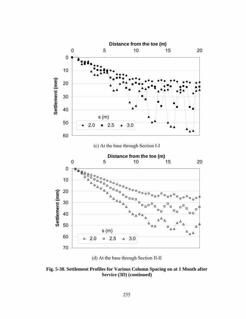
255

0

10

20

30

40

50

60

0 5 10 15 20Distance from the toe (m)

Settl

emen

t (m

m)

2.0 2.5 3.0

s (m)

(c) At the base through Section I-I

0

10

20

30

40

50

60

70

0 5 10 15 20Distance from the toe (m)

Settl

emen

t (m

m)

2.0 2.5 3.0s (m)

(d) At the base through Section II-II

Fig. 5-38. Settlement Profiles for Various Column Spacing on at 1 Month after Service (3D) (continued)

256

0

5

10

15

20

25

30

35

40

10 12 14 16 18 20Distance from the toe (m)

Settl

emen

t (m

m)

2.0 2.5 3.0s (m)

(a) On the crest through Section I-I

0

5

10

15

20

25

30

35

40

10 12 14 16 18 20Distance from the toe (m)

Settl

emen

t (m

m)

2.0 2.5 3.0s (m)

(b) On the crest through Section II-II

Fig. 5-39. Settlement Profiles for Various Column Spacing on at 4.5 Years after Service (3D)

257

0

10

20

30

40

50

60

70

0 5 10 15 20Distance from the toe (m)

Settl

emen

t (m

m)

2.0 2.5 3.0

s (m)

(c) At the base through Section I-I

0

10

20

30

40

50

60

70

0 5 10 15 20

Distance from the toe (m)

Settl

emen

t (m

m)

2.0 2.5 3.0

s (m)

(d) At the base through Section II-II Fig. 5-39. Settlement Profiles for Various Column Spacing on at 4.5 Years after

Service (3D) (continued)

258

The influences of the column spacing on the maximum settlement and the maximum

differential settlement are plotted in Figs. 5-40 and 5-41, respectively. Both the

maximum settlement and the maximum differential settlement increased with the

increase of the column spacing. It is also shown that the column spacing had more

effect on the maximum settlement and the maximum differential settlement at the

base than those on the crest. Figures 5-40 and 5-41 show that the effect of the

consolidation on the maximum settlement and maximum differential settlement when

the column spacing increased.

0

10

20

30

40

50

60

70

2 2.5 3Column spacing (m)

Max

imum

set

tlem

ent (

mm

)

1 month after service (crest)4.5 years after service (crest)1 month after service (base)4.5 years after service (base)

Fig. 5-40. Maximum Settlement versus Column Spacing (3D)

259

0

5

10

15

20

25

30

35

40

2 2.5 3

Column spacing (m)

Max

imum

diff

eren

tial s

ettle

men

t (m

m)

1 month after service (crest)4.5 years after service (crest)1 month after service (base)4.5 years after service (base)

Fig. 5-41. Maximum Differential Settlement versus Column Spacing (3D)

0

0.1

0.2

0.3

0.4

0.5

0.6

0.7

2 2.2 2.4 2.6 2.8 3Column spacing (m)

Max

imum

dis

torti

on (%

)

1 month after service4.5 years after service

Fig. 5-42. Maximum Distortion on the Crest versus Column Spacing (3D)

260

The influence of the column spacing on the maximum distortion is presented in Fig.

5-42. Obviously, the column spacing had a significant influence on the maximum

distortion, i.e., the maximum distortion almost increased linearly with the column

spacing within the range investigated. However, the maximum distortion decreased

with the consolidation, especially for larger spacing.

Influence of Geosynthetic Tensile Stiffness

Different from the 2D parametric study, the geosynthetic reinforcement in the 3D

analysis was modeled as plane triangular elements, connected through nodes. In

addition, the geosynthetic was assumed to be an isotropic material. The influences of

the tensile stiffness on the settlement profiles are presented in Fig. 5-43 and 5-44.

Zero tensile stiffness represents the case without any geosynthetic reinforcement. The

settlement profiles show that the use of the reinforcement with higher tensile stiffness

yielded less maximum and differential settlements. The maximum reduction in the

settlement for the tensile stiffness varying from 0 to 10000kN/m tensile was

approximately 6mm, which is equivalent to 26% reduction. The maximum settlement

and the settlement reduction on the crest occurred in the middle of the half crest.

261

0

5

10

15

20

25

10 12 14 16 18 20Distance from the toe (m)

Settl

emen

t (m

m) 0 1000 5000 10000

J (kN/m)

(a) On the crest through Section I-I

0

5

10

15

20

25

10 12 14 16 18 20

Distance from the toe (m)

settl

emen

t (m

m)

0 1000 5000 10000J (kN/m)

(b) On the crest through Section II-II

Fig. 5-43. Settlement Profiles for Various Tensile Stiffness at 1 Month after Service (3D)

262

0

10

20

30

40

50

0 5 10 15 20Distance from the toe (m)

Settl

emen

t (m

m)

0 1000 5000 10000J (kN/m)

(c) At the base through Section I-I

0

10

20

30

40

50

0 5 10 15 20

Distance from the toe (m)

Settl

emen

t (m

m)

0 1000 5000 10000J (kN/m)

(d) At the Base through Section II-II

Fig. 5-43. Settlement Profiles for Various Tensile Stiffness at 1 Month after Service (3D) (continued)

263

0

5

10

15

20

25

30

10 12 14 16 18 20Distance from the toe (m)

settl

emen

t (m

m)

0 1000 5000 10000J (kN/m)

(a) On the crest through Section I-I

0

5

10

15

20

25

30

10 12 14 16 18 20Distance from the toe (m)

Settl

emen

t (m

m)

0 1000 5000 10000J (kN/m)

(b) On the crest through Section II-II

Fig. 5-44. Settlement Profiles for Various Tensile Stiffness at 4.5 Years after Service (3D)

264

0

10

20

30

40

50

0 5 10 15 20Distance from the toe (m)

Settl

emen

t (m

m) 0 1000 5000 10000

J (kN/m)

(c) At the base through Section I-I

0

10

20

30

40

50

0 5 10 15 20Distance from the toe (m)

Settl

emen

t (m

m) 0 1000 5000 10000

J (kN/m)

(d) At the base through Section II-II

Fig. 5-44. Settlement Profiles for Various Tensile Stiffness at 4.5 Years after Service (3D) (continued)

265

The maximum settlement and differential settlements are plotted against the

reinforcement tensile stiffness in Figs. 5-45 and 5-46, respectively. It is shown that

the geosynthetic reinforcement reduced the maximum settlement and differential

settlements but the reduction was limited.

0

10

20

30

40

50

0 2000 4000 6000 8000 10000Tensile stiffness (kN/m)

Max

imum

set

tlem

ent (

mm

) 1 month after service (crest)4.5 after service (crest)1 month after service (base)4.5 years after service (base)

Fig. 5-45. Maximum Settlement versus Tensile Stiffness (3D)

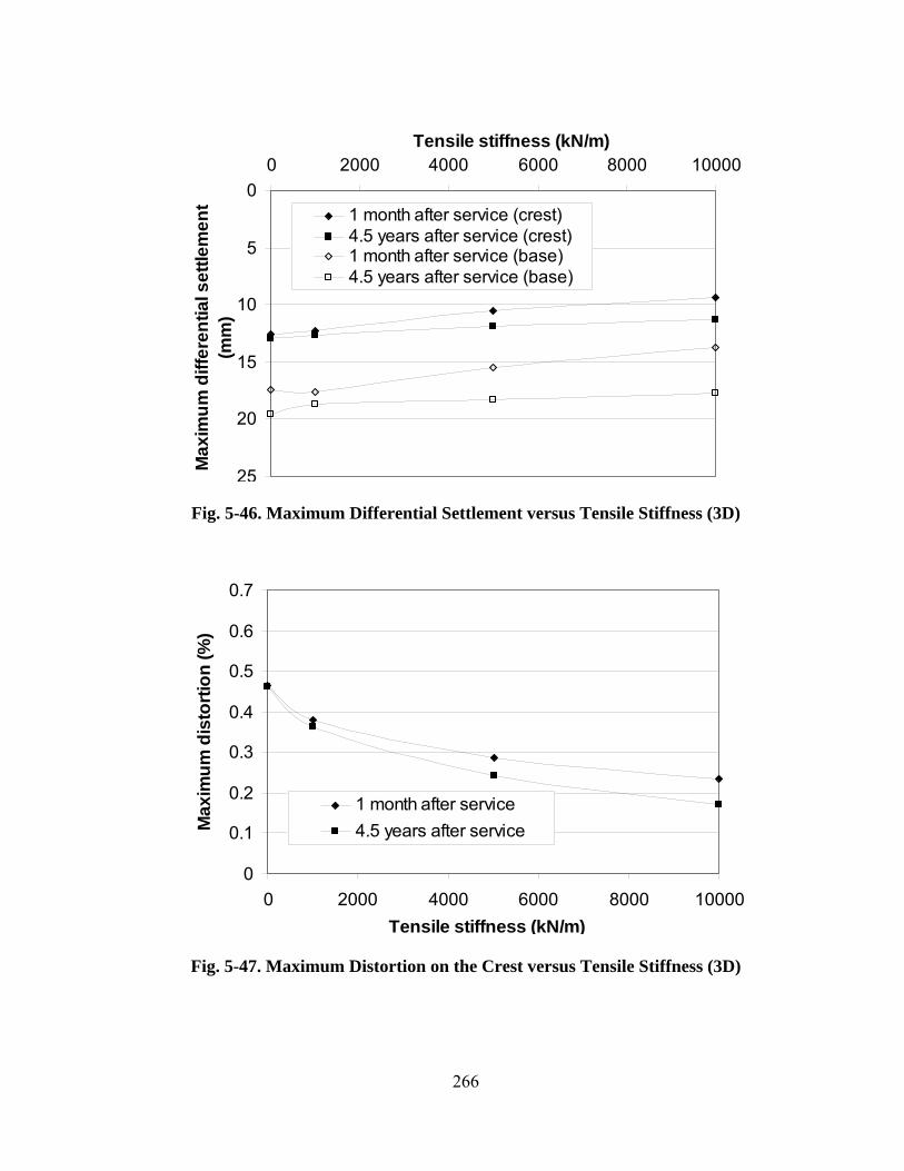
266

0

5

10

15

20

25

0 2000 4000 6000 8000 10000Tensile stiffness (kN/m)

Max

imum

diff

eren

tial s

ettle

men

t (m

m)

1 month after service (crest)4.5 years after service (crest)1 month after service (base)4.5 years after service (base)

Fig. 5-46. Maximum Differential Settlement versus Tensile Stiffness (3D)

0

0.1

0.2

0.3

0.4

0.5

0.6

0.7

0 2000 4000 6000 8000 10000Tensile stiffness (kN/m)

Max

imum

dis

torti

on (%

)

1 month after service4.5 years after service

Fig. 5-47. Maximum Distortion on the Crest versus Tensile Stiffness (3D)

267

The influence of the reinforcement tensile stiffness on the maximum distortion on the

crest is shown in Fig. 5-47. The reduction of the maximum distortion by the

reinforcement with higher stiffness was obvious. The consolidation of the foundation

led to a further reduction on the maximum distortion.

Influence of Construction Rate

The average construction rate was changed in this study to evaluate its influence on

the settlement. The settlement profiles developed under different construction rates

are shown in Figs. 5-48 and 5-49. As expected, the higher construction rate caused a

greater settlement on the crest. At the base, however, the higher construction rate led

to a larger settlement on the soil but a smaller settlement on the columns. This result

is consistent with that found in the 2D parametric study. In addition, the higher

average construction rate led to a greater settlement increase from one month to 4.5

years after service due to higher accumulation of excess pore water pressure. The

detailed discussion on the excess pore water pressure will be presented in the pore

water pressure section.

268

0

5

10

15

20

25

30

35

10 12 14 16 18 20Distance from the toe (m)

Settl

emen

t (m

m)

4 1 0.25v (meter/mon)

(a) On the crest through Section I-I

0

5

10

15

20

25

30

35

10 12 14 16 18 20Distance from the toe (m)

Settl

emen

t (m

m)

4 1 0.25v (meter/mon)

(b) On the crest through Section II-II

Fig. 5-48. Settlement Profiles for Various Average Construction Rates at 1 Month after Service (3D)

269

0

10

20

30

40

50

0 5 10 15 20Distance from the toe (m)

Settl

emen

t (m

m)

4 1 0.25v (meter/mon)

(c) At the base through Section I-I

0

10

20

30

40

50

0 5 10 15 20Distance from the toe (m)

Settl

emen

t (m

m) 4 1 0.25

v (meter/mon)

(d) At the base through Section II-II

Fig. 5-48. Settlement Profiles for Various Average Construction Rates at 1 Month after Service (3D) (continued)

270

0

5

10

15

20

25

30

35

10 12 14 16 18 20

Distance from the toe (m)

Settl

emen

t (m

m)

4 1 0.25v (meter/mon)

(a) On the crest through Section I-I

0

5

10

15

20

25

30

35

10 12 14 16 18 20Distance from the toe (m)

Settl

emen

t (m

m)

4 1 0.25v (meter/mon)

(b) On the crest through Section II-II

Fig. 5-49. Settlement Profiles for Various Average Construction Rates at 4.5 Years after Service (3D)

271

0

10

20

30

40

50

60

0 5 10 15 20Distance from the toe (m)

Settl

emen

t (m

m)

4 1 0.25v (meter/mon)

(c) At the base through Section I-I

0

10

20

30

40

50

60

0 5 10 15 20Distance from the toe (m)

Settl

emen

t (m

m)

4 1 0.25v (meter/mon)

(d) At the base through Section II-II

Fig. 5-49. Settlement Profiles for Various Average Construction Rates at 4.5 Years after Service (3D) (continued)

272

The maximum settlement and differential settlements against the average construction

rate are plotted in Figs. 5-50 and 5-51. The decrease of the average construction rate

led to smaller maximum settlement and differential settlements. The efficiency of the

reduction in the maximum settlement and differential settlements by decreasing the

average construction rate was almost linearly from 4mter/mon to 1meter/mon and

also from 1meter/mon to 0.25meter/mon.

0

10

20

30

40

50

60

0 1 2 3 4Average construction rate (day/meter)

Max

imum

set

tlem

ent (

mm

)

1 month after service (crest)4.5 years after service (crest)1 month after service (base)4.5 years after service (base)

Fig. 5-50. Maximum Settlement versus Average Construction Rate (3D)

273

0

5

10

15

20

25

30

0 1 2 3 4Average construction rate (day/meter)

Max

imum

diff

eren

tial s

ettle

men

t(m

m)

1 month after service (crest)4.5 years after service (crest)1 month after service (base)4.5 years after service (base)

Fig. 5-51. Maximum Differential Settlement versus Average Construction Rate (3D)

0

0.1

0.2

0.3

0.4

0.5

0.6

0.7

0 1 2 3 4Average construction rate (day/meter)

Max

imum

dis

torti

on (%

)

1 month after service4.5 years after service

Fig. 5-52. Maximum Distortion on the Crest versus Average Construction Rate (3D)

274

The influence of the average construction rate on the maximum distortion is presented

in Fig. 5-52. The higher average construction rate resulted in a greater maximum

distortion. The consolidation after the construction did not have much influence on

the maximum distortion.

5.2.3 Tension Developed in Geosynthetics

As discussed previously, the tension in the geosynthetic reinforcement is induced by

the differential settlement between columns and soft soil and the lateral spreading of

the embankment. The influence of various factors on the tension in the geosynthetic

reinforcement was investigated in this study and some of the results are presented

herein.

Influence of Soft Soil Elastic Modulus

Since the geosynthetic reinforcement was simulated as plane elements, the tension

developed in two perpendicular x and y directions can be calculated. The influence of

soil modulus on the maximum tension developed in these two directions is presented

in Fig. 5-53. The x-direction was perpendicular to the traffic direction and the y-

direction was parallel to the traffic direction. Within the range of the soil modulus

investigated in this study, the maximum tension in the x-direction was always higher

275

than that in the y direction. It can be seen that the soil modulus had a considerable

influence on the tension in both directions. The increase of the soil modulus reduced

the maximum tension. Since the increase of the soil modulus reduced the maximum

differential settlement, the geosynthetic sheet was less deformed and stretched so that

the maximum tension was reduced. However, the consolidation of the foundation soil

had an insignificant influence on the maximum tension in both x and y directions as

shown in Fig. 5-53.

0

2

4

6

8

10

12

1 2 3 4 5 6 7 8Soil modulus (MPa)

Max

imum

tens

ion

(kN

/m)

1 month after service (x)4.5 years after service (x)1 month after service (y)4.5 years after service (y)

Fig. 5-53. Maximum Tension versus Soil Modulus (3D)

Influence of Soft Soil Friction Angle

The influence of the soft soil friction angle on the maximum tension in the

reinforcement is shown in Fig. 5-54. The maximum tension in the x direction was

276

higher than that in the y direction. An increase of the soil friction angle reduced the

maximum tension in both directions. The consolidation of the foundation had an

insignificant effect on the maximum tension in both directions.

0

2

4

6

8

10

15 20 25 30Friction angle (o)

Max

imum

tens

ion

(kN

/m)

1 month after service (x)4.5 years after service (x)1 month after service (y)4.5 years after service (y)

Fig. 5-54. Maximum Tension versus Friction Angle (3D)

Influence of Soft Soil Permeability

The influence of the soft soil permeability on the maximum tension in the

geosynthetic reinforcement is shown in Fig. 5-55. The lower soil permeability yielded

higher maximum tension because the lower soil permeability produced higher

maximum differential settlement at the base.

277

0

2

4

6

8

10

0 20 40 60 80 100Soil permeability (x10-10m/s)

Max

imum

tens

ion

(kN

/m)

1 month after service (x)4.5 years after service (x)1 month after service (y)4.5 years after service (y)

Fig. 5-55. Maximum Tension versus Soil Permeability (3D)

Influence of Column Elastic Modulus

The influence of the column modulus on the maximum tension is presented in Fig. 5-

56. Apparently, the maximum tension in the x direction was higher than that in the y

direction. The increase of the column modulus reduced the tension in the geosynthetic

because the increase of the column modulus reduced the maximum differential

settlement. However, the effect of the column modulus on the maximum tension was

smaller in the y direction than that in the x direction. The consolidation of the

foundation had an insignificant effect on the maximum tension in the geosynthetic.

278

0

2

4

6

8

200 300 400 500Column modulus (MPa)

Max

imum

tens

ion

(kN

/m)

1 month after service (x)4.5 years after service (x)1 month after service (y)4.5 years after service (y)

Fig. 5-56. Maximum Tension versus Column Modulus (3D)

Influence of Column Spacing

The influence of the column spacing on the maximum tension in the geosynthetic is

presented in Fig. 5-57, which shows that the maximum tension in the y direction was

lower than that in the x direction and larger spacing led to higher maximum tension in

both x and y directions. The higher maximum tension at larger column spacing

resulted from the larger maximum differential settlement. Figure 5-57 shows that the

time effect on the maximum tension was minimal.

279

0

2

4

6

8

10

12

14

2 2.5 3Column spacing (m)

Max

imum

tens

ion

(kN

/m)

1 month after service (x)4.5 years after service (x)1 month after service (y)4.5 years after service (y)

Fig. 5-57. Maximum Tension versus Column Spacing (3D)

Influence of Geosynthetic Tensile Stiffness

The influence of the geosynthetic tensile stiffness on the maximum tension in both x

and y directions is presented in Fig. 5-58. Since the geosynthetic was modeled as an

isotropic material in this study, the tensile stiffness in both direction was equal. An

increase of the tensile stiffness led to an increase in the maximum tension in both x

and y directions, which is consistent with the phenomenon identified in the 2D

parametric study. However, the increase of the maximum tension in the x direction

was greater than that in the y direction. In addition, the time effect on the maximum

tension was not significant.

280

0

10

20

30

40

50

0 2000 4000 6000 8000 10000Tensile stiffness (kN/m)

Max

imum

tens

ion

(kN

/m)

1 month after service (x)4.5 years after service (x)1 month after service (y)4.5 years after service (y)

Fig. 5-58. Maximum Tension versus Tensile Stiffness (3D)

Influence of Construction Rate

The influence of the average construction rate on thee maximum tension is presented

in Fig. 5-59, which shows the increase of the maximum tension in both x and y

directions with an increase of the average construction rate. In other words, the lower

construction rate yielded the lower maximum tension.

281

0

2

4

6

8

10

0 1 2 3 4Average construction rate (meter/mon)

Max

imum

tens

ion

(kN

/m)

1 month after service (x)4.5 years after service (x)1 month after service (y)4.5 years after service (y)

Fig. 5-59. Maximum Tension versus Average Construction Rate (3D)

5.2.4 Vertical Stress and Stress Concentration Ratio

Similar to the 2D study, the stress concentration ratio, n, was used as an index to

evaluate the efficiency of load transfer from the soft soil to the columns. In the 3D

analysis, the average additional vertical effective stresses on the column and the soft

soil within the influence area were used to calculate the stress concentration ratio.

282

Influence of Soft Soil Elastic Modulus

The influence of the soil modulus on the additional vertical effective stress profiles

along Sections I-I and II-II are presented in Fig. 5-60 and 5-61. The maximum

additional vertical effective stress in Section I-I is much higher than that in Section II-

II, since the DM columns are located at Section I-I. The increase of the soft soil

modulus reduced the additional vertical effective stress on the columns, which is

shown in Fig. 5-60 (a), but increased the additional vertical effective stress in the soft

soil, which is more clearly shown in Fig 5-60 (b).

0

100

200

300

400

500

600

700

800

900

0 5 10 15 20Distance from the toe (m)

Add

ition

al v

ertic

al e

ffect

ive

stre

ss(k

Pa)

1 2 4 8Es (MPa)

(a) Through Section I-I

Fig. 5-60. Additional Vertical Effective Stress Profiles for Various Soil Moduli at 1 Month after Service (3D)

283

0

10

20

30

40

50

60

70

80

0 5 10 15 20Distance from the toe (m)

Add

ition

al v

ertic

al e

ffect

ive

stre

ss (k

Pa)

1 2 4 8Es (MPa)

(b) Through Section II-II Fig. 5-60. Additional Vertical Effective Stress Profiles for Various Soil Moduli at

1 Month after Service (3D) (continued)

0

100200

300

400500

600

700800

900

0 5 10 15 20Distance from the toe (m)

Add

ition

al v

ertic

al e

ffect

ive

stre

ss (k

Pa)

1 2 4 8Es (MPa)

(a) Through Section I-I

Fig. 5-61. Additional Vertical Effective Stress Profiles for Various Soil Moduli at 4.5 Years after Service (3D)

284

0

10

20

30

40

50

60

70

80

0 5 10 15 20Distance from the toe (m)

Add

ition

al v

ertic

al e

ffect

ive

stre

ss(k

Pa)

1 2 4 8Es (MPa)

(b) Through Section II-II

Fig. 5-61. Additional Vertical Effective Stress Profiles for Various Soil Moduli at 4.5 Years after Service (3D) (continued)

For a clearer demonstration, the stress concentration ratio is plotted against the

distance from the toe of the embankment in Fig. 5-62. The higher soft soil modulus

led to a lower stress concentration ratio. The consolidation of the foundation slightly

increased the stress concentration ratio.

285

0

5

10

15

20

25

30

35

0 5 10 15 20Distance from the toe (m)

Stre

ss c

once

ntra

tion

ratio

1 2 4 8

Es (MPa)

(a) 1 month after service

0

5

10

15

20

25

30

35

0 5 10 15 20Distance from the toe (m)

Stre

ss c

once

ntra

tion

ratio

1 2 4 8Es (MPa)

(b) 4.5 years after service

Fig. 5-62. Stress Concentration Ratio Profiles for Various Soil Moduli (3D)

286

Influence of Soft Soil Friction Angle

The influence of the soil friction angle on the additional vertical effective stress is

presented in Fig. 5-63. An increase of the soil friction angle reduced the additional

vertical effective stress on the columns but increased the additional vertical effective

stress in the soil. This finding is in agreement with that in the 2D parametric study in

Chapter Four. The comparison of the profiles at one month after service with those at

4.5 years after service shows negligible change in the additional vertical effective

stress.

0

100

200

300

400

500

600

700

800

900

0 5 10 15 20Distance from the toe (m)

Add

ition

al v

ertic

al e

ffect

ive

stre

ss(k

Pa)

15 20 25 30φ (o)

(a) Through Section I-I

Fig. 5-63. Additional Vertical Effective Stress Profiles of Various Friction Angles at 1 Month after Service (3D)

287

0

10

20

30

40

50

60

70

0 5 10 15 20Distance from the toe (m)

Add

ition

al v

ertic

al e

ffect

ive

stre

ss (k

Pa)

15 20 25 30φ (o)

(b) Through Section II-II

Fig. 5-63. Additional Vertical Effective Stress Profiles of Various Friction Angles at 1 Month after Service (3D) (continued)

0

100

200

300

400

500

600

700

800

900

0 5 10 15 20Distance from the toe (m)

Add

ition

al v

ertic

al e

ffect

ive

stre

ss (k

Pa)

15 20 25 30φ (o)

(a) Through Section I-I Fig. 5-64. Additional Vertical Effective Stress Profiles for Various Friction

Angles at 4.5 Years after Service (3D)

288

0

10

20

30

40

50

60

70

0 5 10 15 20Distance from the toe (m)

Add

ition

al v

ertic

al e

ffect

ive

stre

ss(k

Pa)

15 20 25 30φ (o)

(b) Through Section II-II

Fig. 5-64. Additional Vertical Effective Stress Profiles for Various Friction Angles at 4.5 Years after Service (3D) (continued)

The influence of the soft soil friction angle on the stress concentration ratio is shown

in Fig. 5-65. The higher stress concentration ratio was reached by a lower friction

angle. This phenomenon is consistent with the change of the addition vertical

effective stress with the soil friction angle. The comparison of Fig. 5-65 (a) and (b)

shows a slight increase in the stress concentration ratio.

289

0

5

10

15

20

25

30

35

0 5 10 15 20Distance from the toe (m)

Stre

ss c

once

ntra

tion

ratio

15 20 25 30φ (o)

(a) 1 month after service

0

5

10

15

20

25

30

35

0 5 10 15 20Distance from the toe (m)

Stre

ss c

once

ntra

tion

ratio

15 20 25 30φ (o)

(b) 4.5 years after service

Fig. 5-65. Stress Concentration Ratio Profiles for Various Soil Friction Angles (3D)

290

Influence of Soft Soil Permeability

The profiles of additional vertical effective stresses at different soil permeability are

presented in Fig. 5-66. The lower soil permeability leads increased the additional

vertical effective stress in the columns.

0

100

200

300

400

500

600

700

800

0 5 10 15 20Distance from the toe (m)

Add

ition

al v

ertic

al e

ffect

ive

stre

ss(k

Pa)

1 10 100k (x10-10m/s)

(a) Through Section I-I

Fig. 5-66. Additional Effective Stress Profiles for Various Soil Permeability at 1 Month after Service (3D)

291

0

10

20

30

40

50

60

0 5 10 15 20Distance from the toe (m)

Add

ition

al v

ertic

al e

ffect

ive

stre

ss (k

Pa)

1 10 100k (x10-10m/s)

(b) Through Section II-II

Fig. 5-66. Additional Effective Stress Profiles for Various Soil Permeability at 1 Month after Service (3D) (continued)

0

100

200

300

400

500

600

700

800

0 5 10 15 20Distance from the toe (m)

Add

ition

al v

ertic

al e

ffect

ive

stre

ss (k

Pa)

1 10 100k (x10-10m/s)

(a) Through Section I-I

Fig. 5-67. Additional Effective Stress Profiles for Various Soil Permeability at 4.5 Years after Service (3D)

292

0

10

20

30

40

50

60

0 5 10 15 20

Distance from the toe (m)

Add

ition

al v

ertic

al e

ffect

ive

stre

ss(k

Pa)

1 10 100k (x10-10m/s)

(b) Through Section II-II

Fig. 5-67. Additional Effective Stress Profiles for Various Soil Permeability at 4.5 Years after Service (3D) (continued)

The stress concentration ratio profiles at different time are presented in Fig. 5-68. At

the low permeability (k=10-10m/s), the stress concentration ratio profile at one month

after service was different from others. When the soil permeability was 10-9 to 10-

8m/s, an increase of the soil permeability reduced the stress concentration ratio. As

permeability equal to 10-10m/s, high excess pore water pressure is induced and a large

portion of embankment load is taken by pore water in soil. Hence, additional vertical

effective stress in columns is low, which leads to a low stress concentration ratio at

some locations. At 4.5 years after service, however, the trend became the same as

others, because as consolidation proceeded, the load taken by pore water was

293

transferred to columns. In addition, the stress concentration ratio at 4.5 years after

service was higher than that at one month after service.

0

5

10

15

20

25

30

0 5 10 15 20Distance from the toe (m)

Stre

ss c

once

ntra

tion

ratio

1 10 100

k (x10-10m/s)

(a) At 1 month after service

0

5

10

15

20

25

30

0 5 10 15 20Distance from the toe (m)

Stre

ss c

once

ntra

tion

ratio

1 10 100k (x10-10m/s)

(b) At 4.5 years after service Fig. 5-68. Stress Concentration Ratio Profiles for Various Soil Permeability (3D)

294

Influence of Column Elastic Modulus

The influence of the column modulus on the additional vertical effective stress

profiles is presented in Fig. 5-69 and 5-70, which show that, the higher column

modulus produced higher additional vertical effective stresses on the columns and

lower additional vertical effective stresses in the soft soil. However, since the column

modulus was much higher than the soft soil modulus, the increase of the column

modulus did not have any significant influence on the load transfer. Consequently, the

additional vertical effective stress on the columns and in the soil did not change

much.

0

100

200

300

400

500

600

700

800

0 5 10 15 20Distance from the toe (m)

Add

ition

al v

ertic

al e

ffect

ive

stre

ss(k

Pa)

247 372 497Ec (MPa)

(a) Through Section I-I

Fig. 5-69. Additional Vertical Effective Stress Profiles for Various Column Moduli at 1 Month after Service (3D)

295

0

10

20

30

40

50

60

0 5 10 15 20Distance from the toe (m)

Add

ition

al v

ertic

al e

ffect

ive

stre

ss (k

Pa)

247 372 497Ec (MPa)

(b) Through Section II-II

Fig. 5-69. Additional Vertical Effective Stress Profiles for Various Column Moduli at 1 Month after Service (3D) (continued)

0

100

200

300

400

500

600

700

800

0 5 10 15 20Distance from the toe (m)

Add

ition

al v

ertic

al e

ffect

ive

stre

ss (k

Pa)

247 372 497Ec (MPa)

(a) Through Section I-I Fig. 5-70. Additional Vertical Effective Stress Profiles for Various Column

Moduli at 4.5 Years after Service (3D)

296

0

10

20

30

40

50

60

0 5 10 15 20Distance from the toe (m)

Add

ition

al v

ertic

al e

ffect

ive

stre

ss(k

Pa)

247 372 497Ec (MPa)

(b) Through Section II-II

Fig. 5-70. Additional Vertical Effective Stress Profiles for Various Column Moduli at 4.5 Years after Service (3D) (continued)

The influence of the column modulus on the stress concentration ratio profiles is

presented in Fig. 5-71. The increase of the column modulus yielded a higher stress

concentration ratio. The increase of the column modulus did not increase the stress

concentration ratio significantly. This result is consistent with the influence of the

column modulus on the additional vertical effective stress. In addition, the stress

concentration ratio increased slightly from one month to 4.5 years after service.

297

0

5

10

15

20

25

30

0 5 10 15 20Distance from the toe (m)

Stre

ss c

once

ntra

tion

ratio

247 372 497Ec (MPa)

(a) 1 month after service

0

5

10

15

20

25

30

0 5 10 15 20Distance from the toe (m)

Stre

ss c

once

ntra

tion

ratio

247 372 497

Ec (MPa)

(b) 4.5 years after service

Fig. 5-71. Stress Concentration Ratio Profiles for Various Column Moduli (3D)

298

Influence of Column Spacing

The influence of the column spacing on the additional vertical effective stress profiles

is shown in Fig. 5-72. As discussed in the 2D parametric study, the change of the

column spacing made it difficult to compare the additional vertical effective stresses

in the columns and in the soil at the same location. As a result, the maximum

additional vertical effective stresses on the columns and in the soil were used for the

comparison. The increase of the column spacing yielded an increase of the additional

vertical effective stresses both on the columns and in the soil.

0

100

200

300

400

500

600

700

800

900

0 5 10 15 20Distance from the toe (m)

Add

ition

al v

ertic

al e

ffect

ive

stre

ss(k

Pa)

2.0 2.5 3.0s (m)

(a) Through Section I-I

Fig. 5-72. Additional Vertical Effective Stress Profiles of Various Column Spacing at 1 Month after Service (3D)

299

0

10

20

30

40

50

60

70

0 5 10 15 20Distance from the toe (m)

Add

ition

al v

ertic

al e

ffect

ive

stre

ss (k

Pa)

2.0 2.5 3.0s (m)

(b) Through Section II-II

Fig. 5-72. Additional Vertical Effective Stress Profiles of Various Column Spacing at 1 Month after Service (3D) (continued)

0100200300400500600700800900

0 5 10 15 20

Distance from the toe (m)

Add

ition

al v

ertic

al e

ffect

ive

stre

ss (k

Pa)

2.0 2.5 3.0s (m)

(a) Through Section I-I Fig. 5-73. Additional Vertical Effective Stress Profiles of Various Column

Spacing at 4.5 Years after Service (3D)

300

0

10

20

30

40

50

60

70

0 5 10 15 20Distance from the toe (m)

Add

ition

al v

ertic

al e

ffect

ive

stre

ss(k

Pa)

2.0 2.5 3.0s (m)

(b) Through Section II-II

Fig. 5-73. Additional Vertical Effective Stress Profiles of Various Column Spacing at 4.5 Years after Service (3D) (continued)

The stress concentration ratio profiles of different column spacing are presented in

Fig. 5-74. It can be seen that the change of the spacing even changed the stress

concentration ratio distribution pattern at the spacing of 2.0m. Since the tendency of

the lateral movement at a smaller column spacing was less, the maximum stress

concentration ratio occurred at the center of the embankment, which was also the

distribution pattern found in the 2D parametric study.

301

0

5

10

15

20

25

30

35

40

45

0 5 10 15 20Distance from the toe (m)

Stre

ss c

once

ntra

tion

ratio 2.0 2.5 3.0

s (m)

(a) 1 month after service

0

5

10

15

20

25

30

35

40

45

0 5 10 15 20Distance from the toe (m)

Stre

ss c

once

ntra

tion

ratio 2.0 2.5 3.0

s (m)

(b) 4.5 years after service Fig. 5-74. Stress Concentration Ratio Profiles for Various Column Spacing (3D)

302

Influence of Geosynthetic Tensile Stiffness

The influence of the geosynthetic tensile stiffness on the additional vertical effective

stress profiles is presented in Fig. 4-75 and 4-76. Overall, the higher tensile stiffness

led to lower additional vertical effective stresses both on the columns and in the soil.

0

100

200

300

400

500

600

700

800

0 5 10 15 20Distance from the toe (m)

Add

ition

al v

ertic

al e

ffect

ive

stre

ss(k

Pa)

0 1000 5000 10000J (kN/m)

(a) Through Section I-I

Fig. 5-75. Additional Vertical Effective Stress Profiles for Various Tensile Stiffness at 1 Month after Service (3D)

303

0

10

20

30

40

50

60

0 5 10 15 20Distance from the toe (m)

Add

ition

al v

ertic

al e

ffect

ive

stre

ss (k

Pa)

0 1000 5000 10000J (kN/m)

(b) Through Section II-II

Fig. 5-75. Additional Vertical Effective Stress Profiles for Various Tensile Stiffness at 1 Month after Service (3D) (continued)

0

10

20

30

40

50

60

0 5 10 15 20Distance from the toe (m)

Add

ition

al v

ertic

al e

ffect

ive

stre

ss (k

Pa)

0 1000 5000 10000J (kN/m)

(a) Through Section I-I

Fig. 5-76. Additional Vertical Effective Stress Profiles for Various Tensile Stiffness at 4.5 Years after Service (3D)

304

0

10

20

30

40

50

60

0 5 10 15 20Distance from the toe (m)

Add

ition

al v

ertic

al e

ffect

ive

stre

ss(k

Pa)

0 1000 5000 10000J (kN/m)

(b) Through Section II-II

Fig. 5-76. Additional Vertical Effective Stress Profiles for Various Tensile Stiffness at 4.5 Years after Service (3D) (continued)

The influence of the geosynthetic tensile stiffness on the stress concentration ratio

profiles is shown in Fig. 5-77. The tensile stiffness of the geosynthetic did not have

any significant influence on the stress concentration ratio in Fig. 5-77. Overall, the

stress concentration ratio decreased with an increase of the tensile stiffness.

305

0

5

10

15

20

25

0 5 10 15 20Distance from the toe (m)

Stre

ss c

once

ntra

tion

ratio

0 1000 5000 10000J (kN/m)

(a) 1 month after service

0

5

10

15

20

25

30

0 5 10 15 20Distance from the toe (m)

Stre

ss c

once

ntra

tion

ratio

0 1000 5000 10000J (kN/m)

(b) 4.5 years after service

Fig. 5-77. Stress Concentration Ratio Profiles for Various Tensile Stiffness (3D)

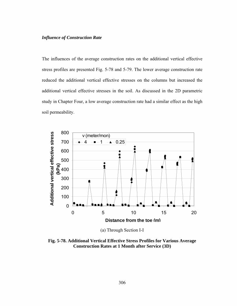
306

Influence of Construction Rate

The influences of the average construction rates on the additional vertical effective

stress profiles are presented Fig. 5-78 and 5-79. The lower average construction rate

reduced the additional vertical effective stresses on the columns but increased the

additional vertical effective stresses in the soil. As discussed in the 2D parametric

study in Chapter Four, a low average construction rate had a similar effect as the high

soil permeability.

0

100

200

300

400

500

600

700

800

0 5 10 15 20Distance from the toe (m)

Add

ition

al v

ertic

al e

ffect

ive

stre

ss(k

Pa)

4 1 0.25v (meter/mon)

(a) Through Section I-I

Fig. 5-78. Additional Vertical Effective Stress Profiles for Various Average Construction Rates at 1 Month after Service (3D)

307

0

10

20

30

40

50

60

0 5 10 15 20Distance from the toe (m)

Add

ition

al v

ertic

al e

ffect

ive

stre

ss (k

Pa)

4 1 0.25v (meter/mon)

(b) Through Section II-II

Fig. 5-78. Additional Vertical Effective Stress Profiles for Various Average Construction Rates at 1 Month after Service (3D) (continued)

0

100

200

300

400

500

600

700

800

0 5 10 15 20Distance from the toe (m)

Add

ition

al v

ertic

al e

ffect

ive

stre

ss (k

Pa)

4 1 0.25v (meter/mon)

(a) Through Section I-I

Fig. 5-79. Additional Vertical Effective Stress Profiles for Various Average Construction Rates at 4.5 Years after Service (3D)

308

0

10

20

30

40

50

60

0 5 10 15 20Distance from the toe (m)

Add

ition

al v

ertic

al e

ffect

ive

stre

ss(k

Pa)

4 1 0.25v (meter/mon)

(b) Through Section II-II

Fig. 5-79. Additional Vertical Effective Stress Profiles for Various Average Construction Rates at 4.5 Years after Service (3D) (continued)

The influence of the average construction rate on the stress concentration ratio

profiles is shown in Fig. 5-80. The increase of the average construction rate led to a

higher stress concentration ratio, which was similar to what had been discussed in 2D

parametric study.

309

0

5

10

15

20

25

30

0 5 10 15 20Distance from the toe (m)

Stre

ss c

once

ntra

tion

ratio

4 1 0.25v (meter/mon)

(a) 1 month after service

0

5

10

15

20

25

30

0 5 10 15 20Distance from the toe (m)

Stre

ss c

once

ntra

tion

ratio

4 1 0.25v (meter/mon)

(b) 4.5 years after service Fig. 5-80. Stress Concentration Ratio Profiles for Various Average Construction

Rates (3D)

310

5.2.5 Excess Pore Water Pressure

As discussed in Chapter Four, under a GRCS embankment, the excess pore water

pressure dissipates hydraulically and mechanically, i.e., through drainage and load

transfer. Therefore, the consolidation process depends on a number of factors in

addition to the soil permeability. The major influence factors were investigated. The

excess pore water pressure distribution within the soft soil along the depth (Section

III-III shown in Fig. 5-1) and the degree of consolidation of the section are used as

representatives.

Influence of Soft Soil Elastic Modulus

The excess pore water pressure distribution along Section III-III (refer to Fig. 5-1) at

one month after service is presented in Fig. 5-81. Since the excess pore water pressure

at 4.5 years after service approached zero, it is not presented in this section. Figure 5-

81 shows that the excess pore water pressure at one month after service increased

with the increase of the soft soil modulus. This phenomenon was identified and

explained in details in the 2D parametric study.

311

0

2

4

6

8

10

12

0 5 10 15 20 25 30

Excess pore water pressure (kPa)

Dep

th (m

)

1248

Es (MPa)

Fig. 5-81. Excess Pore Water Pressure Distributions for Various Soil Moduli (3D)

Following the same approach used in Chapter Four, the degree of consolidation at one

month after service was calculated and plotted against the soil modulus as shown in

Fig. 5-82. It can be concluded that higher soil modulus led to a lower degree of

consolidation. Within the investigated range of the soft soil modulus, the degree of

consolidation varied approximately 6%, which implies that the soft soil modulus had

a limited influence on the degree of consolidation. Furthermore, the influence of the

soil modulus on the degree of consolidation became less as the soil modulus

increased.

312

70

75

80

85

90

95

100

1 2 3 4 5 6 7 8Soil modulus (MPa)

Deg

ree

of c

onso

lidat

ion

(%)

Fig. 5-82. Degree of Consolidation versus Soil Modulus (3D)

Influence of Soft Soil Friction Angle

The excess pore water pressure distribution along Section III-III is presented in Fig.

5-83. The smaller friction angle resulted in less excess pore water pressure at one

month after service. This phenomenon is also consistent with that found in the 2D

parametric study in Chapter Four. The difference in the excess pore water pressures at

different friction angles was too small to make any practical significance.

313

0

2

4

6

8

10

12

0 5 10 15 20 25 30Excess pore water pressure (kPa)

Dep

th (m

)

15 20 25 30φ (o)

Fig. 5-83. Excess Pore Water Pressure Distributions for Various Friction Angles (3D)

70

75

80

85

90

95

100

15 20 25 30Friction angle (o)

Deg

ree

cons

olid

atio

n (%

)

Fig. 5-84. Degree of Consolidation versus Friction Angle (3D)

314

The degree of consolidation is plotted in Fig. 5-84 for a clearer illustration of the

influence of the soil friction angle on the excess pore water pressure. The smaller soil

friction angle led to a slightly higher degree of consolidation.

Influence of Soft Soil Permeability

The influence of the soil permeability on the excess pore water pressure distribution

along Section III-III is shown in Fig. 5-85. As expected, the higher soil permeability

led to less pore water pressure. The excess pore water pressure at one month of

service almost dissipated completely at the soil permeability of 10-8m/s.

0

2

4

6

8

10

12

0 10 20 30 40 50 60Excess pore water pressure (kPa)

Dep

th (m

)

110100

k (x10-10m/s)

Fig. 5-85. Excess Pore Water Pressure Distributions for Various Soil Permeability (3D)

315

70

75

80

85

90

95

100

0 20 40 60 80 100Soil permeability (x10-10m/s)

Deg

ree

of c

onso

lidat

ion

(%)

(a) Permeability in a normal scale

70

75

80

85

90

95

100

1 10 100Soil permeability (x10-10m/s) (log scale)

Deg

ree

of c

onso

lidat

ion

(%)

(b) Permeability in a log scale

Fig. 5-86. Degree of Consolidation versus Soil Permeability (3D)

316

The degree of consolidation is plotted with respect to the soil permeability in Fig. 5-

86. It can be seen that the soil permeability had a remarkable influence on the degree

of consolidation. As shown in Fig. 5-86 (b), the degree of consolidation increased

almost linearly with respect to the log scale of the soil permeability.

Influence of Column Elastic Modulus

The influence of the column modulus on the excess pore water pressure distribution

along Section III-III is shown in Fig. 5-87. Apparently, the higher column modulus

resulted in the lower the excess pore water pressure. This phenomenon can be

explained that more excess pore water pressure dissipated by transferring the load

from the soil to the columns when the column modulus was higher. Detailed

discussion on this phenomenon can be found in Chapter Four.

The degree of consolidation is plotted against the column modulus in Fig. 5-88. The

higher column modulus led to a higher degree of consolidation.

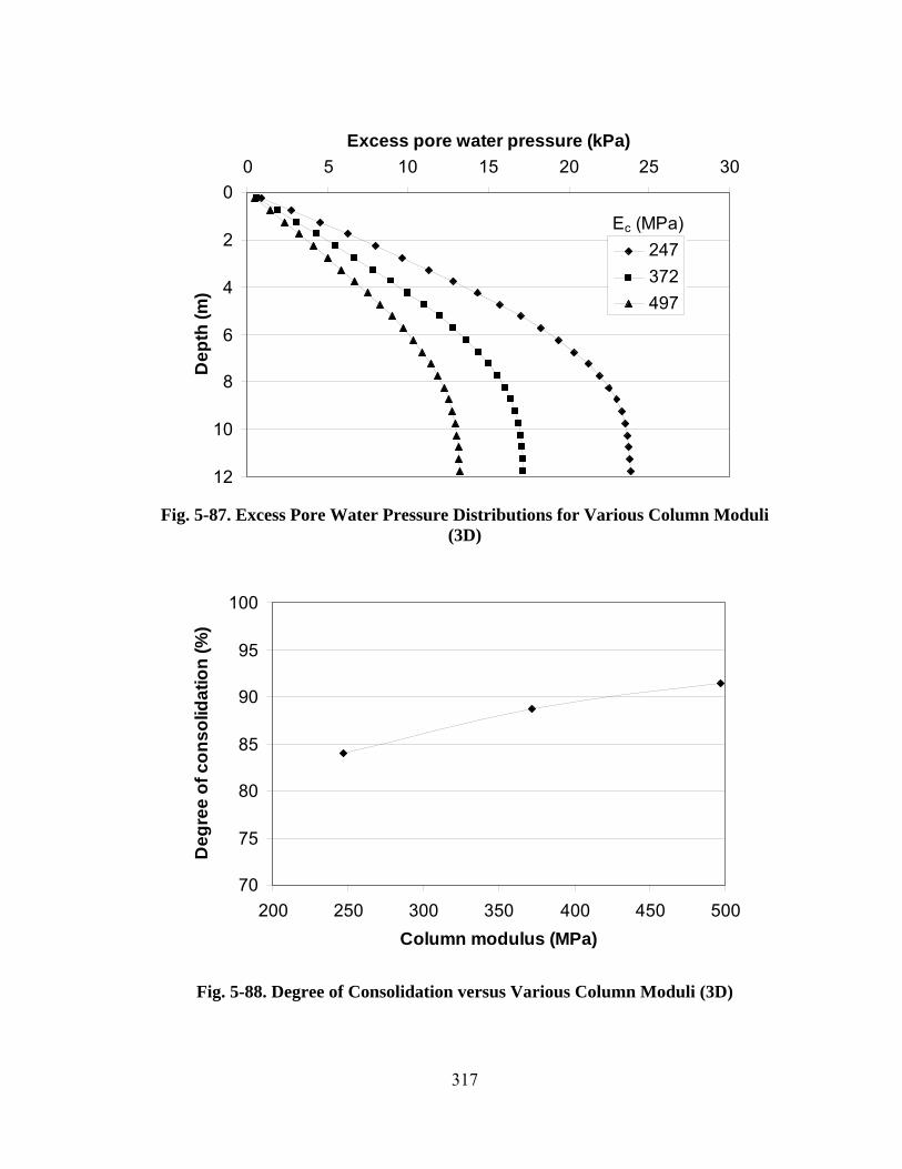
317

0

2

4

6

8

10

12

0 5 10 15 20 25 30Excess pore water pressure (kPa)

Dep

th (m

)

247372497

Ec (MPa)

Fig. 5-87. Excess Pore Water Pressure Distributions for Various Column Moduli (3D)

70

75

80

85

90

95

100

200 250 300 350 400 450 500Column modulus (MPa)

Deg

ree

of c

onso

lidat

ion

(%)

Fig. 5-88. Degree of Consolidation versus Various Column Moduli (3D)

318

Influence of Column Spacing

The influence of the column spacing on the excess pore water pressure distribution

along Section III-III is presented in Fig. 5-89. The larger column spacing led to a

higher excess pore water pressure. This finding is consistent with that found in the 2D

parametric study.

0

2

4

6

8

10

12

0 5 10 15 20 25 30Excess pore water pressure (kPa)

Dep

th (m

)

2.02.53.0

s (m)

Fig. 5-89. Excess Pore Water Pressure Distributions for Various Column Spacing (3D)

The degree of consolidation is plotted against the column spacing in Fig. 5-90. Larger

column spacing resulted in less degree of consolidation.

319

70

75

80

85

90

95

100

2 2.5 3Column spacing (m)

Deg

ree

cons

olid

atio

n (%

)

Fig. 5-90. Degree of Consolidation versus Column Spacing (3D)

Influence of Geosynthetic Tensile Stiffness

The influence of the geosynthetic tensile stiffness on the excess pore water pressure

distribution along Section III-III is presented in Fig. 5-91. The increase of the tensile

stiffness led to a slightly higher excess pore water pressure. The reason for the

difference can be found in details in Chapter Four.

The degree of consolidation versus the geosynthetic tensile stiffness is presented in

Fig. 5-92. The degree of consolidation decreases slightly with the increase of the

geosynthetic tensile stiffness.

320

0

2

4

6

8

10

12

0 5 10 15 20 25 30Excess pore water pressure (kPa)

Dep

th (m

)

01000500010000

J (kN/m)

Fig. 5-91. Excess Pore Water Pressure Distributions for Various Tensile Stiffness (3D)

70

75

80

85

90

95

100

0 2000 4000 6000 8000 10000Tensile stiffness (kN/m)

Deg

ree

of c

onso

lidat

ion

(%)

Fig. 5-92. Degree of Consolidation versus Tensile Stiffness (3D)

321

Influence of Construction Rate

The influence of the excess pore water pressure distribution along Section III-III is

presented in Fig. 5-93, which shows that the less excess pore water pressure

accumulated at the lower average construction rate. As mentioned earlier, some of the

excess pore water pressure dissipated during the construction. As the average

construction rate was lower, more time was allowed for the excess pore pressure to

dissipate during the construction.

0

2

4

6

8

10

12

0 10 20 30 40Excess pore water pressure (kPa)

Dep

th (m

)

410.25

v (meter/mon)

Fig. 5-93. Excess Pore Water Pressure Distributions for Various Average Construction Rates (3D)

The degree of consolidation is plotted with respect to the average construction rate in

Fig. 5-94. The lower average construction rate yielded the higher degree of

consolidation.

322

70

75

80

85

90

95

100

0 1 2 3 4Average construction rate (meter/mon)

Deg

ree

of c

onso

lidat

ion

(%)

Fig. 5-94. Degree of Consolidation versus Average Construction Rate (3D)

323

CHAPTER SIX

COMPARISON OF TWO-DIMENSIONAL AND THREE

DIMENSIONAL STUDIES

Detailed 2D and 3D parametric study results have been presented in Chapters Four

and Five, respectively. The results of the 2D and 3D parametric studies are

summarized and compared in this chapter for two purposes. One is to evaluate the

validity of the approach converting 3D cases into 2D cases based on their weighted

areas. The column modulus in the 3D study was converted from the corresponding

column modulus used in the 2D study and the other parameters were kept the same as

those used in the 2D study. In practice, this weighted-area converting approach is

commonly used to simplify columns installed in a square pattern to walls so that

solutions or software for 2D problems can be used. To the author’s best knowledge,

however, this validity has been rarely verified. The second purpose of the comparison

is to summarize and rate the influence of the investigated factors on the settlement,

the tension, the stress concentration ratio, and the pore water pressure.

6.1 Verification of Simplified Modeling

Three-dimensional modeling is much more complicated and time-consuming than 2D

modeling. Therefore, it is common practice to simplify a 3D case into a 2D case. One

324

approach is to convert columns installed in a square pattern into walls based on a

weighted area. Opposite to this procedure, walls can be converted to columns if the

pattern of columns is known or assumed. As discussed in Chapter Five, the column

moduli in the 3D parametric study were converted from those used in the 2D

parametric study. For example, the column modulus of 247MPa under the 3D

condition was converted from the wall modulus of 100MPa under the 2D condition.

The 2D modeling in this research terminated at 30 years after service, at which the

degree of consolidation reached 100%. The status at 30 years after service is

considered as the final status of the 2D modeling. Even though the 3D modeling

terminated at 4.5 years after service, most of the excess pore water pressures

dissipated and the degrees of consolidation were more than 95%. Therefore, the status

at 4.5 years after service is approximately taken as the final status of the 3D

modeling. The 2D and 3D results at one month after service and at the final status are

both compared but an emphasis is on the results for the final status. The maximum

settlements against the column moduli at one month after service and at the final

status are presented in Fig. 6-1 (a) and (b), respectively. It is shown that the 2D

results had the same maximum settlement trends on the crest and at the base with the

increase of the modulus as the 3D results. However, the 2D results overestimated the

maximum settlement both on the crest and at the base as compared with the 3D

results. In addition, the maximum distortion is plotted against the column modulus in

Fig. 6-2, which shows that the 2D results underestimated the maximum distortion at

325

one month after service and the final status as compared with the 3D results. These

comparisons show the differences in the maximum settlement and distortion between

the converted 2D cases and the corresponding 3D ones.

0

10

20

30

40

50

100 150 200

Column modulus (MPa)

Max

imum

set

tlem

ent (

mm

) on the crest (2D)at the base (2D)on the crest (3D)at the base (3D)

(a) 1 month after service

Fig. 6-1. Comparison of Maximum Settlement

326

0

10

20

30

40

50

60

100 150 200

Column modulus (MPa)

Max

imum

set

tlem

ent (

mm

) on the crest (2D)at the base (2D)on the crest (3D)at the base (3D)

(b) Final status

Fig. 6-1. Comparison of Maximum Settlement (continued)

0.1

0.2

0.3

0.4

0.5

0.6

0.7

100 150 200Column modulus (MPa)

Max

imum

dis

torti

on (%

)

2D (1 month) 2D (Final)3D (1 month) 3D (Final)

Fig. 6-2. Comparison of Maximum Distortion

327

The maximum tension in the geosynthetic reinforcement against the column modulus

is plotted in Fig. 6-3. The legends, “3D (X, one month)” and “3D (Y, one month)”,

represent the tension developed in the x and y directions, respectively at one month

after service while “3D (X, final)” and “3D (Y, final)” represent the tension

developed in the x and y directions, respectively at the final status. Figure 6-3 shows

that the maximum tension obtained from the 2D modeling deviated from that from

the 3D modeling except when the column modulus was close to 100MPa. It is also

shown that the tension in the y direction was much lower than that in the x direction.

0

2

4

6

8

10

12

100 150 200Column modulus (MPa)

Max

imum

tens

ion

(kN

/m) 2D (1 month) 2D (final)

3D (X, 1 month) 3D (X,final)3D (Y, 1 month) 3D (Y,final)

Fig. 6-3. Comparison of Maximum Tension

The maximum stress concentration ratio is plotted against the column modulus in Fig.

6-4. It is expected that the 2D cases underestimated the maximum stress

328

concentration ratio as compared with the corresponding 3D cases since the column

moduli in the 2D cases were lower than those in the corresponding 3D cases.

0

10

20

30

40

50

100 150 200Column modulus (MPa)

Max

imum

stre

ss c

once

ntra

tion

ratio

2D (1 month) 2D (final)3D (1 month) 3D (final)

Fig. 6-4. Comparison of Maximum Stress Concentration Ratio

The degree of consolidation at one month after service is plotted against the column

modulus in Fig. 6-5 to evaluate the difference in the excess pore water pressure. The

2D cases underestimated the degree of consolidation as compared with the

corresponding 3D cases.

329

60

70

80

90

100

100 150 200Column modulus (MPa)

Deg

ree

of c

onso

lidat

ion

(%) 2D

3D

Fig. 6-5. Comparison of Degree of Consolidation

On the basis of the above comparisons, a general conclusion can be made: the

simplified 2D model can not well compute the maximum settlement, the maximum

distortion, the maximum tension, the maximum stress concentration ratio, and the

degree of consolidation if the columns are actually arranged in a 3D pattern, such as

the square pattern in this study.

6.2 2D and 3D Comparisons

Even though the influence of each factor on the performance of GRCS embankments

has been discussed in Chapter Four for the 2D modeling and Chapter Five for the 3D

330

modeling, they have not been summarized and well compared. Hence, the 2D and 3D

results would be summarized, compared, and rated herein. In this section, both the

results at one month after service and at the final status are presented, however, the

results at the final status are used as the bases for the comparisons.

6.2.1 Maximum Settlement and Distortion

The settlement is the key issue for the performance of the GRCS embankments,

especially the maximum and differential settlements on the crest. To evaluate the

influence of each factor on the maximum and differential settlements, the maximum

settlement and distortion on the crest of the embankment are used.

Influence of Soft Soil Elastic Modulus

The maximum settlement and distortion under 2D and 3D conditions are plotted

against the soil modulus in Fig. 6-6 and Fig. 6-7, respectively. Figure 6-6 shows that

although the maximum settlement under the 3D condition was smaller than that under

the 2D condition, the degrees of influence under these two conditions were almost the

same. The maximum settlement was reduced by about 20mm under both conditions

when the soil modulus increased from 1 to 8MPa.

331

10

20

30

40

50

1 2 3 4 5 6 7 8Soil modulus (MPa)

Max

imum

set

tlem

ent (

mm

)

2D (1 month) 2D (final)3D (1 month) 3D (final)

Fig. 6-6. Maximum Settlement versus Soil Modulus under 2D and 3D Conditions

The maximum distortion at the crest is presented against the soil modulus in Fig. 6-7.

Apparently, the increase of the soil modulus had more effect on the reduction of the

maximum distortion under the 3D condition than that under the 2D condition. When

the soil modulus increased from 1 to 8MPa, the maximum distortion under the 3D

condition decreased by about 0.4%, while the maximum distortion under the 2D

condition decreased by about 0.3%.

332

0.1

0.2

0.3

0.4

0.5

0.6

0.7

1 2 3 4 5 6 7 8

Soil modulus (MPa)

Max

imum

dis

torti

on (%

) 2D (1 month) 2D (final)3D (1 month) 3D (final)

Fig. 6-7. Maximum Distortion versus Soil Modulus under 2D and 3D Conditions

Influence of Soft Soil Friction Angle

The maximum settlement and distortion against the soil friction angle are presented in

Figs. 6-8 and 6-9, respectively. Apparently, the increase of the soil friction angle had

a greater effect on the reduction in the maximum settlement and especially the

maximum distortion under the 3D condition than those under the 2D condition. When

the soil friction angle increased from 15o to 30o, the maximum settlement under the

3D condition was reduced by 15mm and the maximum distortion was reduced by

0.4%, while the maximum settlement under the 2D condition was reduced by 10mm

and the maximum distortion was reduced by 0.1%. These differences are attributed to

the sliding of the embankment fill. The embankment constructed above the columns

333

installed in a square pattern had a higher tendency of sliding than that above the

walls. Unlike the 2D condition, the columns in a square pattern were isolated by the

soft soil. The sliding surface extending into the foundation could cut through the soft

soil without intersecting with any DM columns. Local failure was more likely to

occur. The increase of the soil strength would minimize the local failure; therefore, it

had a remarkable influence on both the maximum settlement and the maximum

distortion.

10

20

30

40

50

15 20 25 30Friction angle (o)

Max

imum

set

tlem

ent (

mm

)

2D (1 month) 2D (final)3D (1 month) 3D (final)

Fig. 6-8. Maximum Settlement versus Friction Angle under 2D and 3D Conditions

334

0.1

0.2

0.3

0.4

0.5

0.6

0.7

15 20 25 30Friction angle (o)

Max

imum

dis

torti

on (%

)

2D (1 month) 2D (final)3D (1 month) 3D (final)

Fig. 6-9. Maximum Distortion versus Friction Angle under 2D and 3D Conditions

Influence of Soft Soil Permeability

The influences of the soil permeability on the maximum settlement and the maximum

distortion are presented in Fig. 6-10 and 6-11, respectively, which show that the

increase of the soil permeability had a significant effect on the reduction of the

maximum settlement and the maximum distortion under both 3D and 2D conditions.

As the soil permeability increased from 10-10m/s to 10-8m/s, the maximum settlement

decreased by approximately 17mm and the maximum distortion decreased by 0.4%

under the 3D condition, while the maximum settlement and the maximum distortion

decreased by about 22mm and 0.2% under the 2D condition, respectively.

335

10

20

30

40

50

0 20 40 60 80 100

Soil permeability (x10-10m/s)

Max

imum

set

tlem

ent (

mm

)

2D (1 month) 2D (final)3D (1 month) 3D (final)

Fig. 6-10. Maximum Settlement versus Soil Permeability under 2D and 3D Conditions

0.1

0.2

0.3

0.4

0.5

0.6

0.7

0 20 40 60 80 100

Soil permeability (x10-10m/s)

Max

imum

dis

torti

on (%

) 2D (1 month) 2D (final)3D (1 month) 3D (final)

Fig. 6-11. Maximum Distortion versus Soil Permeability under 2D and 3D Conditions

336

Influence of Column Elastic Modulus

The influences of the column modulus on the maximum settlement and the maximum

distortion under both 3D and 2D conditions are shown in Fig. 6-12 and 6-13,

respectively. The increase of the column modulus had an effect on the reduction in

the maximum settlement and the maximum distortion. However, this effect was

limited under both 3D and 2D conditions. An increase of the column modulus from

100MPa to 200MPa reduced the maximum settlement and the maximum distortion by

about 8mm and 0.03%, respectively under the 3D condition, and by 6mm and 0.01%,

respectively under the 2D condition.

10

20

30

40

50

100 150 200

Column modulus (MPa)

Max

imum

set

tlem

ent (

mm

)

2D (1 month) 2D (final)3D (1 month) 3D (final)

Fig. 6-12. Maximum Settlement versus Column Modulus under 2D and 3D Conditions

337

0.1

0.2

0.3

0.4

0.5

0.6

0.7

100 150 200Column modulus (MPa)

Max

imum

dis

torti

on (%

)2D (1 month) 2D (Final)3D (1 month) 3D (Final)

Fig. 6-13. Maximum Distortion versus Column Modulus under 2D and 3D Conditions

Influence of Column Spacing

The maximum settlement and the maximum distortion against the column spacing are

presented in Fig. 6-14 and 6-15, respectively. As the column spacing increased from

2m to 3m, the maximum settlement increased about 20mm and 17mm under the 3D

and 2D conditions, respectively while the maximum distortion increased about 0.35%

and 0.19% under the 3D and 2D conditions, respectively.

338

10

20

30

40

50

2 2.5 3Column spacing (m)

Max

imum

set

tlem

ent (

mm

)

2D (1 month) 2D (final)3D (1 month) 3D (final)

Fig. 6-14. Maximum Settlement versus Column Spacing under 2D and 3D Conditions

0.1

0.2

0.3

0.4

0.5

0.6

0.7

2 2.5 3Column spacing (m)

Max

imum

dis

torti

on (%

) 2D (1 month) 2D (final)3D (1 month) 3D (final)

Fig. 6-15. Maximum Distortion versus Column Spacing under 2D and 3D Conditions

339

Influence of Geosynthetic Tensile Stiffness

The maximum settlement and the maximum distortion are plotted against the

geosynthetic tensile stiffness in Figs. 6-16 and 6-17, respectively, which show that the

geosynthetic tensile stiffness had an limited effect on the maximum settlements under

both 3D and 2D conditions. The maximum settlements decreased by approximately

2mm under 3D and 2D conditions as the tensile stiffness increased from 0 to

10,000kN/m. However, the geosynthetic tensile stiffness had a significant influence

on the maximum distortion under the 3D condition but an insignificant influence on

the maximum distortion under the 2D condition. When the geosynthetic tensile

stiffness varied from 0 to 10,000kN/m, the maximum distortion decreased by 0.3%

under the 3D condition but only by 0.02% under the 2D condition. This discrepancy

is also attributed to the local deformation between individual columns or walls.

Hence, the tendency of the local deformation can be mitigated by the geosynthetic

reinforcement. The geosynthetic with the higher tensile stiffness had more effect on

the mitigation.

340

10

20

30

40

50

0 2000 4000 6000 8000 10000Tensile stiffness (kN/m)

Max

imum

set

tlem

ent (

mm

)

2D (1 month) 2D (final)3D (1 month) 3D (final)

Fig. 6-16. Maximum Settlement versus Tensile Stiffness under 2D and 3D Conditions

0.1

0.2

0.3

0.4

0.5

0.6

0.7

0 2000 4000 6000 8000 10000

Tensile stiffness (kN/m)

Max

imum

dis

torti

on (%

) 2D (1 month) 2D (final)3D (1 month) 3D (final)

Fig. 6-17. Maximum Distortion versus Tensile Stiffness under 2D and 3D Conditions

341

Influence of Construction Rate

The influences of the average construction rate on the maximum settlement and the

maximum distortion are presented in Figs. 6-18 and 6-19, respectively. As the

average construction rate decreased from 4 to 0.25meter/mon, the maximum

settlement decreased by 12mm under the 3D condition and by 15mm under the 2D

condition while the maximum distortion decreased by 0.32% under the 3D condition

and 0.1% under the 2D condition, respectively.

10

20

30

40

50

0 1 2 3 4

Average construction rate (meter/mon)

Max

imum

set

tlem

ent (

mm

)

2D (1 month) 2D (final)3D (1 month) 3D (final)

Fig. 6-18. Maximum Settlement versus Average Construction Rate under 2D and 3D Conditions

342

0.1

0.2

0.3

0.4

0.5

0.6

0.7

0 1 2 3 4Average construction rate (meter/mon)

Max

imum

dis

torti

on (%

)

2D (1 month) 2D (final)3D (1 month) 3D (final)

Fig. 6-19. Maximum Distortion versus Average Construction Rate under 2D and

3D Conditions

6.2.2 Maximum Tension Developed in Geosynthetics

The tension calculated under the 2D condition was that developed along the direction

perpendicular to the traffic direction. Under the 3D condition, the tension developed

in the direction along the traffic (i.e., the y direction) and perpendicular to the traffic

(i.e., the x direction) can be calculated. Since the maximum tension in x direction

under the 3D condition is corresponding to that in the 2D condition, the maximum

tension in the x direction under the 3D condition was used for comparison with that

under the 2D condition.

343

Influence of Soft Soil Elastic Modulus

The influence of the soil modulus on the maximum geosynthetic tension is presented

in Fig. 6-20, which shows that for the soil modulus from 1 to 8MPa, the maximum

tension in the x and y directions decreased by 7kN/m and 4kN/m, respectively under

3D condition instead of 8kN/m under the 2D condition.

0

2

4

6

8

10

12

1 2 3 4 5 6 7 8Soil modulus (MPa)

Max

imum

tens

ion

(kN

/m)

2D (1 month) 2D (final)3D (X, 1 month) 3D (X,final)3D (Y, 1 month) 3D (Y,final)

Fig. 6-20. Maximum Tension versus Soil Modulus under 2D and 3D Conditions

Influence of Soft Soil Friction Angle

The maximum geosynthetic tension is plotted against the soft soil friction angle in

Fig. 6-21. For the soil friction angle from 15o to 30o, the maximum tension in the x

344

and y directions decreased by 4kN/m and 2kN/m, respectively, under the 3D

condition instead of slightly more than 2kN/m under the 2D condition.

0

2

4

6

8

10

12

15 20 25 30Friction angle (o)

Max

imum

tens

ion

(kN

/m)

2D (1 month) 2D (final)3D (X, 1 month) 3D (X, final)3D (Y, 1 month) 3D (Y, final)

Fig. 6-21. Maximum Tension versus Friction Angle under 2D and 3D Conditions

Influence of Soft Soil Permeability

The influence of the soil permeability on the maximum geosynthetic tension is

presented in Fig. 6-22. As the soil permeability increased from 10-10 to 10-8m/s, the

maximum tension in the x and y directions both decreased by about 3kN/m under the

3D condition instead of about 4kN/m under the 2D condition.

345

0

2

4

6

8

10

12

0 20 40 60 80 100Soil permeability (x10-10m/s)

Max

imum

tens

ion

(kN

/m)

2D (1 month) 2D (final)3D (X, 1 month) 3D (X,final)3D (Y, 1 month) 3D (Y,final)

Fig. 6-22. Maximum Tension versus Soil Permeability under 2D and 3D Conditions

Influence of Column Elastic Modulus

Figure 6-23 presents the relationship between the maximum tension and the column

modulus, which shows that the column modulus had limited influence on the

maximum tension. However, the influence of the column modulus on the maximum

tension in the x direction under the 3D condition was more significant than those

under other conditions.

346

0

2

4

6

8

10

12

100 150 200Column modulus (MPa)

Max

imum

tens

ion

(kN

/m) 2D (1 month) 2D (final)

3D (X, 1 month) 3D (X,final)3D (Y, 1 month) 3D (Y,final)

Fig. 6-23. Maximum Tension versus Column Modulus under 2D and 3D Conditions

Influence of Column Spacing

The influence of the column spacing on the maximum tension is presented in Fig. 6-

24. As the column spacing increased from 2 to 3m, the maximum tension in the x

and y directions decreased by approximately 8kN/m and 4kN/m, respectively, under

the 3D condition instead of approximately 5kN/m under the 2D condition.

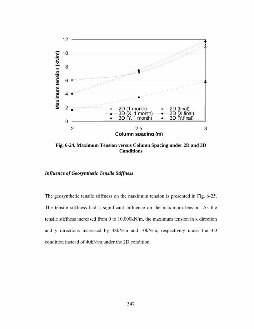
347

0

2

4

6

8

10

12

2 2.5 3Column spacing (m)

Max

imum

tens

ion

(kN

/m)

2D (1 month) 2D (final)3D (X, 1 month) 3D (X,final)3D (Y, 1 month) 3D (Y,final)

Fig. 6-24. Maximum Tension versus Column Spacing under 2D and 3D Conditions

Influence of Geosynthetic Tensile Stiffness

The geosynthetic tensile stiffness on the maximum tension is presented in Fig. 6-25.

The tensile stiffness had a significant influence on the maximum tension. As the

tensile stiffness increased from 0 to 10,000kN/m, the maximum tension in x direction

and y directions increased by 48kN/m and 10kN/m, respectively under the 3D

condition instead of 40kN/m under the 2D condition.

348

0

10

20

30

40

50

0 2000 4000 6000 8000 10000

Tensile stiffness (kN/m)

Max

imum

tens

ion

(kN

/m)

2D (1 month) 2D (final)3D (X, 1 month) 3D (X,final)3D (Y, 1 month) 3D (Y,final)

Fig. 6-25. Maximum Tension versus Tensile Stiffness under 2D and 3D Conditions

Influence of Construction Rate

The maximum geosynthetic tension against the average construction rate is shown in

Fig. 6-26. The maximum tension in the x and y directions decreased by

approximately 3kN/m and 2kN/m, respectively under the 3D condition when the

average construction rate was decreased from 4 to 0.25meter/mon. The maximum

tension decreased by about 3kN/m in the same range of the average construction rate

under the 2D condition.

349

0

2

4

6

8

10

12

0 1 2 3 4

Average construction rate (meter/mon)

Max

imum

tens

ion

(kN

/m)

2D (1 month) 2D (final)3D (X, 1 month) 3D (X,final)3D (Y, 1 month) 3D (Y,final)

Fig. 6-26. Maximum Tension versus Average Construction Rate under 2D and 3D Conditions

6.2.3 Maximum Stress Concentration ratio

The stress concentration ratio was adopted in this study to evaluate the load transfer

efficiency. The stress concentration ratios under 2D and 3D conditions have been

discussed in Chapter Four and Chapter Five, respectively. They are presented here

together for the purpose of comparison.

350

Influence of Soft Soil Elastic Modulus

The maximum stress concentration ratio against the soil modulus is presented in Fig.

6-27, which shows that the soil modulus had a remarkable influence on the maximum

stress concentration under both 3D and 2D conditions. For the soil modulus varying

from 1 to 8MPa, the maximum stress concentration ratio decreased by 20 and 25

under 3D and 2D conditions, respectively.

0

10

20

30

40

50

1 2 3 4 5 6 7 8Soil modulus (MPa)

Max

imum

stre

ss c

once

ntra

tion

ratio

2D (1 month) 2D (final)3D (1 month) 3D (final)

Fig. 6-27. Maximum Stress Concentration Ratio versus Soil Modulus under 2D

and 3D Conditions

351

Influence of Soft Soil Friction Angle

The maximum stress concentration ratios developed at different soil friction angles

under 2D and 3D conditions are presented in Fig. 6-28. For the soil friction angle

ranging from 15o to 30o, the maximum stress concentration ratio decreased by 10

under the 3D condition and by 6 under the 2D condition.

0

10

20

30

40

50

15 20 25 30Friction angle (o)

Max

imum

stre

ss c

once

ntra

tion

ratio

2D (1 month) 2D (final)3D (1 month) 3D (final)

Fig. 6-28. Maximum Stress Concentration Ratio versus Friction Angle under 2D

and 3D Conditions

Influence of Soft Soil Permeability

The maximum stress concentration ratio is plotted against the soft soil permeability in

Fig. 6-29. The increase of the soil permeability from 10-10 to 10-8m/s led to a decrease

352

of the maximum stress concentration ratio by 9 under the 3D condition and by 15

under the 2D condition.

0

10

20

30

40

50

0 20 40 60 80 100Soil permeability (x10-10m/s)

Max

imum

stre

ss c

once

ntra

tion

ratio

2D (1 month) 2D (final)3D (1 month) 3D (final)

Fig. 6-29. Maximum Stress Concentration Ratio versus Soil Permeability under

2D and 3D Conditions

Influence of Column Elastic Modulus

The maximum stress concentration ratio versus the column modulus is presented in

Fig. 6-30. The increase of the column modulus from 100 to 200MPa led to an in

crease in the maximum stress concentration ratio of 4 and 5 under 3D and 2D

conditions, respectively.

353

0

10

20

30

40

50

100 150 200Column modulus (MPa)

Max

imum

stre

ss c

once

ntra

tion

ratio

2D (1 month) 2D (final)3D (1 month) 3D (final)

Fig. 6-30. Maximum Stress Concentration Ratio versus Column Modulus under

2D and 3D Conditions

Influence of Column Spacing

The curves of the maximum stress concentration ratio versus the column spacing are

shown in Fig. 6-31. When the column spacing was increased from 2m to 3m, the

maximum stress concentration ratio decreased by approximately 20 and 17 under 3D

and 2D conditions, respectively.

354

0

10

20

30

40

50

2 2.5 3

Column spacing (m)

Max

imum

stre

ss c

once

ntra

tion

ratio

2D (1 month) 2D (final)3D (1 month) 3D (final)

Fig. 6-31. Maximum Stress Concentration Ratio versus Column Spacing under

2D and 3D Conditions

Influence of Geosynthetic Tensile Stiffness

The maximum stress concentration ratio is plotted against the tensile stiffness in Fig.

6-32. Clearly, the tensile stiffness had a slight influence on the stress concentration

ratio. For the tensile stiffness varying from 0 to 10000kN/m, the maximum stress

concentration ratio only decreased by approximately 1 and 3 under 3D and 2D

conditions, respectively.

355

0

10

20

30

40

50

0 2000 4000 6000 8000 10000

Tensile stiffness (kN/m)

Max

imum

stre

ss c

once

ntra

tion

ratio

2D (1 month) 2D (final)3D (1 month) 3D (final)

Fig. 6-32. Maximum Stress Concentration Ratio versus Tensile Stiffness under 2D and 3D Conditions

Influence of Construction Rate

The influence of the average construction rate on the maximum stress concentration

ratio is presented in Fig. 6-33. As the average construction rate decreased from 4 to

0.25meter/mon, the maximum stress concentration ratio decreased by approximately

6 and 7 under 3D and 2D conditions, respectively.

356

0

10

20

30

40

50

0 1 2 3 4Average construction rate (meter/mon)

Max

imum

stre

ss c

once

mtra

tion

ratio

2D (1 month) 2D (final)3D (1 month) 3D (final)

Fig. 6-33. Maximum Stress Concentration Ratio versus Average Construction Rate under 2D and 3D Conditions

6.2.4 Excess Pore Water Pressure

The comparisons conduced on the maximum settlement, the maximum distortion, the

maximum tension, and the maximum stress concentration ratio were based on the

results at one month of service and the final status. However, the comparison of the

excess pore water pressure is based on the results at one month after service because

the excess pore water pressure at the final status completely dissipated under the 2D

condition and almost completely dissipated under the 3D condition.

357

Influence of Soft Soil Elastic Modulus

The influence of the soil modulus on the degree of consolidation is presented in Fig.

6-34. The increase of the soil modulus from 1 to 8MPa resulted in the decrease in the

degree of consolidation by approximately 6% and 5% under 3D and 2D conditions,

respectively.

60

70

80

90

100

1 2 3 4 5 6 7 8Soil modulus (MPa)

Deg

ree

of c

onso

lidat

ion

(%)

2D3D

Fig. 6-34. Degree of Consolidation versus Soil Modulus under 2D and 3D Conditions

Influence of Soft Soil Friction Angle

The degree of consolidation is plotted against the soil friction angle in Fig. 6-35. The

increase of the soil friction angle yielded a slight decrease in the degree of

consolidation.

358

60

70

80

90

100

15 20 25 30

Friction angle (o)

Deg

ree

of c

onso

lidat

ion

(%)

2D3D

Fig. 6-35. Degree of Consolidation versus Friction Angle under 2D and 3D Conditions

Influence of Soft Soil Permeability

The influence of the soil permeability on the degree of consolidation is presented in

Fig. 6-36. The increase of the soil permeability had a dramatic influence on the

degree of consolidation. As the soil permeability increased from 10-10 to 10-8m/s, the

degree of consolidation increased by approximately 30% and 38% under 3D and 2D

conditions. For the soft soil at the permeability of 10-8m/s, the degree of

consolidation at one month of service was nearly 100% at both 2D and 3D conditions.

359

60

70

80

90

100

0 20 40 60 80 100Soil permeability (x10-10m/s)

Deg

ree

of c

onso

lidat

ion

(%)

2D3D

Fig. 6-36. Degree of Consolidation versus Soil Permeability under 2D and 3D Conditions

Influence of Column Elastic Modulus

The influence of the column modulus on the degree of consolidation versus is shown

in Fig. 6-37. The increase of the column modulus from 100 to 200MPa resulted in an

increase of the degree of consolidation by 8% and 10% under 3D and 2D conditions,

respectively.

360

60

70

80

90

100

100 120 140 160 180 200Column modulus (MPa)

Deg

ree

of c

onso

lidat

ion

(%) 2D

3D

Fig. 6-37. Degree of Consolidation versus Column Modulus under 2D and 3D Conditions

Influence of Column Spacing

The influence of the column spacing on the degree of consolidation is presented in

Fig. 6-38. The increase of the column spacing from 2 to 3m led to a decrease in the

degree of consolidation by 6% and 5% under 3D and 2D conditions, respectively.

361

60

70

80

90

100

2 2.5 3

Column spacing (m)

Deg

ree

of c

onso

lidat

ion

(%)

2D3D

Fig. 6-38. Degree of Consolidation versus Column Spacing under 2D and 3D Conditions

Influence of Geosynthetic Tensile Stiffness

The degree of consolidation is presented against the geosynthetic tensile stiffness in

Fig. 6-39. The increase of the tensile stiffness from 0 to 10,000kN/m only led to a

decrease in the degree of consolidation by about 1% under the 3D condition and

about 2% under the 2D condition.

362

60

70

80

90

100

0 2000 4000 6000 8000 10000

Tensile stiffness (kN/m)

Deg

ree

of c

onso

lidat

ion

(%) 2D

3D

Fig. 6-39. Degree of Consolidation versus Tensile Stiffness under 2D and 3D Conditions

Influence of Construction Rate

The degree of consolidation is plotted against the average construction rate in Fig. 6-

40. As the average construction rate decreased from 4 to 0.25meter/mon, the degree

of consolidation increased by approximately 15% under the 3D condition and by 23%

under the 2D condition.

363

60

70

80

90

100

0 1 2 3 4

Average construction rate (meter/mon)

Deg

ree

of c

onso

lidai

ton

(%)

2D3D

Fig. 6-40. Degree of Consolidation versus Average Construction Rate under 2D

and 3D Conditions

6.2.5 Summary

The influences of various factors on the maximum settlement, the maximum

distortion, the maximum tension, the maximum stress concentration ratio, and the

degree of consolidation under 3D and 2D conditions have been compared above. To

help the design of GRCS embankments, the influences of the factors are summarized

and rated below.

The influence of a factor on the behavioral parameters related to the performance of

the GRCS embankment (including the maximum settlement, the maximum distortion,

364

the maximum tension, the maximum stress concentration ratio, and the degree of

consolidation) is considered positive or negative according to its influence on the

serviceability of the GRCS embankment. If the increase of the factor leads to a

decrease in the maximum settlement, the maximum distortion or maximum tension,

this factor is considered having a positive effect on any of these behavioral

parameters; otherwise, this factor is considered having a negative effect on the

behavioral parameter. On the other hand, if the increase of the factor leads to an

increase in the maximum stress concentration ratio or degree of consolidation, this

factor is considered having a positive effect on any of these behavioral parameters;

otherwise, this factor is considered having a negative effect on the behavioral

parameters. For example, by increasing the soil modulus the maximum settlement

decreases, and maximum stress concentration ratio decreases, then the soil modulus is

defined to have a positive influence on maximum settlement but a negative influence

on maximum stress concentration ratio. The degree of influence of each influence

factor on any of the behavioral parameters is defined as ratio of the variation of the

behavioral parameter to the mean of the behavioral parameter. For example, under 2D

conditions, the maximum settlements at soft soil modulus equal to 1, 2, 4, and 8MPa

are 34.69, 24.79, 20.25, and 14.87mm, respectively. The variation of the maximum

settlement within the soft soil modulus range investigated is 82.1987.1469.34 =−

and the mean of the maximum settlement is 78.242

87.1469.34=

+ . Consequently, the

degree of influence of soft soil modulus on the maximum settlement is calculated as

365

%80%10078.2482.19

=× . The degree of influence on the behavioral parameters is listed

in Table 6-1 and 6-2.

Table 6-1. The Degree of Influence under a 3D Condition (%)

Factors Smax Imax Tmax nmax UmaxEs 68 120 102 176 7 φ 47 87 30 34 1 k 58 81 44 31 35 Ec 14 9 24 18 8 s 75 86 97 60 6 J 14 92 168 8 2 v 51 76 32 22 19

Table 6-2. The Degree of Influence under a 2D Condition (%)

Factors Smax Imax Tmax nmax UmaxEs 66 100 131 299 6 φ 25 21 39 25 3 k 68 73 54 88 46 Ec 24 9 3 24 12 s 49 57 57 74 6 J 8 13 173 29 3 v 47 23 37 45 28

The degree of the influence on any of the behavioral parameters is divided into three

levels: high, medium, and low. Since there is no standard to distinguish those levels,

the common concept of the significance in geotechnical engineering is adopted, i.e.,

the degree of influence less than 30% is considered low; the degree of influence

between 30% and 60% is considered medium and the degree of influence greater than

60% is considered high.

366

The influence of each factor on each behavioral parameter is presented in Table 6-3

and 6-4. The negative sign (-) indicates negative influence and the positive sign (+)

indicates positive influence. The number of negative or positive sign indicates the

degree of influence. One sign indicates low influence; two signs indicates medium

influence; three signs indicates high influence. For example, one positive sign, i.e.,

“+”, indicates low positive influence; two negative signs, i.e., “- -”, indicates medium

negative influence.

Table 6-3. The Influence of Factors under the 3D Condition

Factors Smax Imax Tmax nmax UmaxEs + + + + + + + + + - - - - φ + + + + + + + - - - k + + + + + + + - - + + Ec + + + + + s - - - - - - - - - - - - - J + + + + - - - - - v - - - - - - - + -

Note: smax – maximum settlement, Imax – maximum distortion, Tmax – maximum tension, nmax – maximum stress concentration ratio, Umax – maximum degree of consolidation.

Table 6-4. The Influence of Factors under the 2D Condition

Factors Smax Imax Tmax nmax Umax Es + + + + + + + + + - - - - φ + + + + - - k + + + + + + + + - - - + + Ec + + + + + s - - - - - - - - - - J + + - - - - - v - - - - - + + -

367

CHAPTER SEVEN

CONCLUSIONS AND RECOMMENDATIONS

In the past twenty years, especially in the last few years, various studies have been

completed on GRCS embankments, which have greatly improved the understanding

of this technology. This study is expected to provide additional knowledge into this

topic. The major findings from this study are summarized in this chapter and

recommendations for practical applications are made. In addition, possible future

studies on this topic are presented at the end of this chapter.

7.1 Conclusions

This research was the first comprehensive study that coupled mechanical and

hydraulic modeling of GRCS embankments. The behavior and performance of the

embankments were investigated in a time domain. This study provided important and

useful information on the post-construction settlement and the generation and

dissipation of excess pore water pressure. The findings from this study are

summarized below.

♦ The total settlement, the differential settlement, and the distortion at the base of the

embankment were much larger than those on the crest for both 2D and 3D cases. It is

368

misleading to use the base values as the reference to evaluate the serviceability of the

GRCS embankment.

♦ When columns were installed in a square pattern, the differential settlement

developed along the direction perpendicular to the traffic direction was much larger

than that along the traffic direction. Therefore, more attention should be paid to the

differential settlement developed in the direction perpendicular to the traffic direction

in practice.

♦ Obvious difference existed in the maximum settlement, the maximum distortion,

the maximum tension, and the degree of consolidation from the 3D and the converted

2D analyses. The simplification of a 3D case into a 2D case based on the area

weighted average approach may not result in a good representation of the 3D case.

♦ The time-dependent settlement on the crest (i.e., post-construction settlement) was

influenced by a number of factors. A coupled mechanical and hydraulic modeling is

preferred to accurately estimate the settlement on the crest.

♦ The consolidation process of the foundation under the GRCS embankment was

much faster than that estimated using Terzaghi’s one-dimensional consolidation

theory because the excess pore water pressure dissipated through drainage and load

transfer.

369

♦ According to the results of 2D and 3D parametric study, all the investigated factors

had some effect on the maximum settlement on the crest. The type of influence by

each factor on the maximum settlement under the 3D condition was the same as that

under the 2D condition. The soft soil modulus had a high positive influence on the

maximum settlement under both 2D and 3D conditions. The soil permeability had a

medium positive influence under 3D condition but a high positive influence under 2D

condition. The soft soil friction angle had a medium positive influence under 3D

condition and had a low positive influence under 2D condition. The column modulus

had a low positive influence under 3D and 2D conditions. The column spacing had a

high and medium negative influence under 3D and 2D conditions, respectively. The

geosynthetic tensile stiffness had a low positive influence under both 3D and 2D

conditions and the average construction rate had a medium negative influence under

both 3D and 2D conditions.

♦ The maximum distortion on the crest is the most important index used to describe

the smoothness of the embankment surface. The influence type of each investigated

factor on the maximum distortion under the 3D condition was same as that under the

2D condition. However, the degree of influence under the 3D condition might differ

from that under the 2D condition. The soft soil modulus and the soft soil permeability

had a high positive effect under both 2D and 3D conditions. The soft soil friction

angle had a high and a low positive influence under 3D and 2D conditions,

370

respectively. The column modulus had a low positive influence under both 2D and

3D conditions. The column spacing had a high negative influence under 3D condition

and a medium negative influence under 2D condition. The geosynthetic tensile

stiffness had a high and low positive influence under 3D and 2D conditions,

respectively. The average construction rate had a high and a low negative influence

under 3D and 2D conditions, respectively.

♦ The maximum tension developed in the geosynthetic reinforcement is an important

parameter in the material selection. Under the 3D condition, the maximum tension

was always developed along the direction that was perpendicular to the traffic

direction. This result was attributed to the lateral movement of the embankment fill.

The investigated factors had the same type of influence on the maximum tension

under both 2D and 3D conditions. All of the investigated factors had the same degree

of influence under 3D conditions as under 2D conditions. The soft soil modulus had

a high positive influence under both 2D and 3D conditions. The soft soil friction

angle and the soft soil permeability had a medium positive influence under both 2D

and 3D conditions. The column modulus had a low positive influence under 2D and

3D conditions. The column spacing had a high and a medium negative influence

under 3D and 2D conditions, respectively. The geosynthetic tensile stiffness had a

high negative influence under both 2D and 3D conditions. And the average

construction rate had a medium negative influence under both 2D and 3D conditions.

371

♦ The stress concentration ratio is used to evaluate the load transfer efficiency. All

the factors had the same type of influence on the maximum stress concentration ratio

under the 3D condition as that under the 2D condition. The soft soil modulus and

column spacing had a high negative influence under both 2D and 3D conditions. The

column modulus had a low positive influence and the geosynthetic tensile stiffness

had a low negative influence under both 2D and 3D conditions. The soft soil friction

angle had a medium negative influence under the 3D condition and a low negative

influence under the 2D condition. The soft soil permeability had a medium negative

influence under the 3D condition but a high negative influence under the 2D

condition. The average construction rate had a low positive influence under the 3D

condition and a medium positive influence under the 2D condition.

♦ The degree of consolidation is used to reflect the magnitude of remaining excess

pore water pressure after service. The influence type of each factor on the degree of

consolidation under the 3D condition was the same as that under the 2D condition.

The degree of consolidation of each influence factor under the 3D condition was the

same as that under the 2D condition. The soft soil modulus, the soft soil friction

angle, the column spacing, the geosynthetic tensile stiffness, and the average

construction rate had low negative influence. The column modulus had low positive

influence and the soft soil permeability had medium positive influence.

372

♦ Among all the factors investigated, the soft soil modulus had a high positive

influence on the maximum settlement, the maximum distortion, and the maximum

tension, while it had a high negative influence on the maximum stress concentration

ratio. It indicates that an increase of soft soil modulus could reduce not only the

maximum settlement, the maximum distortion, and the maximum tension but also the

required strength of DM columns.

♦ The geosynthetic tensile stiffness only had a high influence on the maximum

tension but had a low influence on the other behavioral parameters under the 2D

condition. This fact indicated that the use of a stiffer geosynthetic reinforcement was

not an effective approach to improve the serviceability of the GRCS embankments

under the 2D condition.

♦ The soft soil permeability had a medium to high influence on the performance

indices under both 2D and 3D conditions. The increase of the soft soil permeability

could reduce the maximum settlement, the maximum distortion, and the maximum

tension but increase the degree of consolidation. In addition, the increase of the soft

soil permeability led to a decrease in the maximum stress concentration ratio. In a

word, the increase of soil permeability could improve the performance of the GRCS

embankments and reduce the required strength of columns.

373

♦ The column modulus had a low influence on all of the behavioral parameters

concerned under both 2D and 3D conditions. On the other hand, the column spacing

had a medium to high influence on the maximum settlement, the maximum distortion,

the maximum tension, and the maximum stress concentration ratio under 2D and 3D

conditions. It implies that the use of a larger area replacement ratio would be more

effective than the use of stronger columns to improve the serviceability of GRCS

embankments.

♦ The soft soil permeability and the average construction rate showed significant

influence on the increase in the maximum settlement after construction. However, the

maximum differential settlement and the maximum distortion did not consistently

increase with consolidation. The variations of the maximum differential settlement

and the maximum distortion were insignificant for the cases analyzed in this study

except for the cases with low permeability (<10-10m/s) or a high construction rate

(>4meter/mon).

♦ The tension in the geosynthetic reinforcement did not vary significantly with the

consolidation after the construction based on the cases investigated in this study

except for the case having low soil permeability (<10-10m/s) or a high construction

rate (> 4m/mon).

374

♦ Lower soil permeability and/or higher construction rate led to an increased

immediate settlement due to induced local failure.

♦ GRCS embankments over columns in a square pattern showed higher tendency of

lateral movement than those over walls.

7.2 Recommendations

The following recommendations can be made from this study:

1. Three-dimensional analyses are recommended when columns are installed in a

square pattern since a converted 2D model may yield inaccurate results.

2. The settlements on the crest of the embankment should be used to evaluate its

serviceability instead of those at the base.

3. It is important to minimize excess pore water pressure developed during the

construction of the embankment since high excess pore water pressure increases not

only the post-construction settlements but also the immediate settlements. A low

construction rate may be adopted to reduce the accumulation of excess pore water

pressure for foundation soils having low permeability.

375

4. Geosynthetic reinforcement should be used when columns are installed in a square

pattern in a large spacing.

7.3 Future Work

The following issues may be considered for future work:

1. Most studies including the study in this dissertation have assumed a pseudo-static

load to simulate the traffic load. It is more realistic to model the traffic load as cyclic

loading, which is expected to have influences on the generation and dissipation of the

excess pore water pressure and the settlement.

2. In addition to the wall and square patterns of columns, the triangular, rectangular,

and wall patterns along the direction perpendicular to the traffic direction are used in

practice. It would be useful to evaluate the effectiveness of these patterns.

3. GRCS embankments may be used with other ground improvement technologies,

such as wick drains. The use of wick drains can accelerate the consolidation process.

This combined technology should be further investigated.

376

4. The installation of columns may lead to disturbance on foundation soil and

generate excess pore water pressure. The generated pore water pressure is expected to

affect the behavior of GRCS embankments. The influence of installation should be

studied in 2D and 3D numerical modeling in the future.

5. In this study, the embankment fill was modeled as a linearly elastic perfectly

plastic material. However, the mechanical properties of the embankment fill are

typically stress-dependent. This effect should be investigated in the future study.

6. In this study, the soft soil was modeled as a linearly elastic perfectly plastic

material. In a future study, Cam-Clay model may be used to investigate the influence

of other factors, such as over consolidation ratio (OCR), ground water table depth and

so on, on GRCS embankment performance.

377

REFERENCES

Agaiby, S. W. and Jones, C. J. F. P. (1995). “Design of reinforced fill systems over

voids” Canadian Geotechnical Journal, 32(6), p 939-945.

Alamgir, M., Miura, N., Poorooshasb, H. B. and Madhav, M. R. (1996).

“Deformation analysis of soft ground reinforced by columnar inclusions.”

Computers and Geotechnics, 18(4), p 267-290.

Alexiew, D. and Gartung, E. (1999). “Geogrid reinforced railway embankment on

piles-performance monitoring 1994-1998.” Proc. of Geossinteticos’ 99, Rio de

Janeiro, Brazil, p 403-411.

Alzamora, D. Wayne, M. H. and Han, J. (2000). “Performance of SRW supported by

geogrids and jet grout columns.” Proceedings of ASCE Specialty Conference on

Performance Confirmation of Constructed Geotechnical Facilities, Geotechnical

Special Publication No. 94, ASCE, p 456-466.

Barksdale, R. D. and Dobson, T. (1983). “Improvement of marginal urban sites using

stone columns and rigid concrete columns.” The 34th Annual Highway Geology

Symposium and Field Trip at Stone Mountain, GA, 16p.

Bedesem, W. B. (1964). A Continuum Theory of Soil-Structure Interaction in

Granular Media. Ph.D. Thesis, University of Illinois-Urbana Champaign.

Bell, A. L., Jenner, C., Maddison, J. D. and Vignoles, J. (1994). “Embankment

support using geogrids with vibro concrete columns.” Proceedings, 5th

378

International Conference on Geotextiles, Geomembranes, and Related Products,

p 335-338.

Biot, M. A. (1956) “General solutions of the equations of elasticity and

Cconsolidation for a porous material.” J. Appl. Mech., Trans. ASME, 78, p 91-96.

Blumel, W., Heinemann, M., Werth, K. and Muller, K. D. (2004). “Road construction

on a landfill with vibro concrete columns and geogrids.” Proc. Euro Geo3,

Geosynthetic Conference, March 1-3, Munich, Germany, p 273-278.

Bonaparte, R. and Christoper, B. (1987). “Design and construction of reinforced

embankments over weak foundations.” Transportation Research Record, n 1153,

p 26-39.

Bonaparte, R., Holtz, R. D. and Giroud, J. P. (1985). “Soil reinforcement design using

geotextiles and geogrids.” ASTM Symposium Geotextile Testing and the Design

Engineering, Los Angeles, Calif., July.

Borges, J. L. and Cardoso, A. S. (2001). “Structural behavior and parametric study of

reinforced embankment on soft clays.” Computer and Geotechnics, 28(3), p 209-

233.

Brandl, H., Gartung, E., Verspohl, J. and Alexiew, D. (1997). “Performance of a

geogrid-reinforced railway embankment on piles.” Proc. of the 14th ICSMFE,

Hamburg, 3, p 1731-1736.

British Standard Institution. (1995). BS8006 Code of Practice for Strengthened/

Reinforced Soils and Other Fills. London, U.K..

379

Broms, B. B. and Wong, I. H. (1985). “Embankment piles.” Third International

Geotechnical Seminar—Soil Improvement Methods, Singapore, Nov. p 27-29.

Bruce, D. A. (2001). An Introduction to the Deep Mixing Methods as Used in

Geotechnical Applications – Volumne III: The Verification and Properties of

Treated Ground. FHWA-RD-99-167, 455p.

Budhu, M. (2000). Soil Mechanics and Foundations. New York: John Wiley, 586p.

Card, G. B. and Carter, G.R. (1995). “Case history of a piled embankment in

London's Docklands.” Engineering Geology of Construction, Geological Society

Engineering Geology Special Publication No. 10, p 79-84.

Carlsson, B. (1987). Reinforced soil, principles for calculation. Terratema AB,

LinkÖping.

Chelapati, C. V. (1964). “Arching in soil due to the deflection of a rigid horizontal

strip.” Technical Note N-591, U.S. Naval Civil Engineering Laboratory, Port

Hueneme, Calif., October.

Chen, R.P., Chen, Y.M., Han, J. and Xu, Z.Z. (2006). “A theoretical solution for pile-

supported embankments on soft soil.” Submitted for possible publication in

Canadian Geotechnical Journal.

Chen, R. P., Chen, Y. M. and Xu, Z. Z. (2006). “Interaction of rigid pile-supported

embankment on soft soil.” Geotechnical Special Publication, n 151, Proceedings

of GeoShanghai Conference, p 231-238.

380

Chen, R. P., Jia, N. and Chen, R. P. (2004). “Soil arching analysis of pile-supported

embankment.” China Journal of Highway and Transportation, 17(4), p 1-6. (in

Chinese)

Chen, Sheng-Li, Zhang, Bing-Yin, Zhang, Jian-Min and Yin, Kun-Ting (2005).

“Centrifugal modeling of reinforced embankment on soft clay.” Yanshilixue Yu

Gongcheng Xuebao/Chinese Journal of Rock Mechanics and Engineering,

24(15), Aug. 1, p 2751-2756. (in Chinese)

Chew, S. H., Phoon, H. L., Loke, K. H. and Lim, L. K. (2004). “Geotextile reinforced

piled embankment for highway bridges.” 8th International Conference on

Advanced Technology on Transportation Engineering, Beijing, China, May 26-

28, p 438-443.

Chow, Y. K. (1996). “Settlement analysis of vertical loaded stone columns in soft

ground.” Soil and Foundation, 36(1), p 111-113.

Cochrane, S. R. and Bell, A. L. (1981). “Settlement behaviour of a test foundation

slab founded on soft clay.” Ground Movements and Structures, Proceedings of

the 2nd International Conference, p 638-654.

Collin, J. G. (2003). Column Supported Embankments Technical Summary # 10, 65p.

Collin, J. G. (2004). “Column supported embankment design consideration.” Proc. of

the 52 Annual Geotechnical Engineering Conference, J.F. Labuz and J.G. Bentler

(eds.) p 51-78.

381

Crowe, R. E., Bathurst, R. J. and Alston, C. (1999). “Design and construction of a

road embankment using geosynthetics.” Canadian Geotechnical Conference, Oct

23-25, Winnipeg, Manit, Canada, p 266-271.

Das, B. M. (2001). Principles of Geotechnical Engineering, fifth edition, Brooks/Cole,

Pacific Grove, CA, 589p.

Demerdash, M. A. (1996). An Experimental Study of Piled Embankments

Incorporating Geosynthetic Basal Reinforcement. Ph.D. Dissertation, University

of Newcastle-Upon-Type, 158p.

Dubois, D. D. and Bell, A. L. (1982). “Fabric reinforced trial embankment.”

Quarterly Journal of Engineering Geology, 15(3), p 217-225.

Dunnicliff, J. (1988). Geotechnical Instrumentation for Monitoring Field

Performance, Wiley, 608p.

EPRI (1990). Manual on Estimating Soil Properties for Foundation Design, Cornell

University, Ithaca, 327p.

Fei, K., Liu, H.-L. and Gao, Y.-F. (2004). “Settlement differential analysis of PCC

rigid pile composite ground under road embankment loading.” Yantu Lixue/Rock

and Soil Mechanics, 25(8), Aug., p 1244-1248. (in Chinese)

Filz, G. M. and Smith, M. E. (2005). Design of Bridging Layers in Geosynthetic-

Reinforced, Column-Supported Embankments, Final Contract Report, 40p.

Finn, W. D. L. (1960). Stresses in Soil Masses under Various Boundary Conditions.

Ph.D. Dissertation, Seattle, the University of Washington.

382

Finn, W. D. L. (1963). “Boundary value problems of soil mechanics.” Journal of the

Soil Mechanics and Foundation Division, ASCE, 89(SM5), p 39-72.

Fluet, J.E., Christopher, B.R. and Slater, A.R. (1986). “Geosynthetic stress-strain

response under embankment loading condition.” Proc. 3rd Int. Conf. on Geotextiles,

Vienna, Vol. 1, p 175-180.

Forsman, J. (2001). Geovahvistetutkimus, Helsinki, 122p (in Finnish).

Forsman, J., Honkala, A. and Smura, M. (1999). “Hertsby case: A column stabilized

and geotextile reinforced road embankment on soft subsoil.” Dry Mix Method for

Deep Soil Stabilization, Bredenberg, Holm, and Broms (eds), Balkema, Rotterdam,

p 263-268.

Gabr, M., Dodson, R. and Collin, J. (1998). “A study of stress distribution in geogrid

reinforced sand.” Geotechnical Special Publication, p 62-76.

Gabr, M. and Han, J. (2005). “Geosynthetic reinforcement for soft foundations: US

perspectives.” Geotechnical Special Publication, Geo-Frontiers, n 130-142, p

3095-3114.

Getzler, Z., Komornik, A. and Mazurik, A. (1968). “Model study on arching above

buried structures.” Journal of the Soil Mechanics and Foundation Division,

ASCE, 94(SM5), p 1123-1141.

Giroud, J. P., Bonaparte, R., Beech, J. F. and Gross, B. A. (1990). “Design of soil

layer-geosynthetic systems overlying voids.” Geotextile and Geomembrane,

Elsevier, 9(1), p 11-50.

383

Goh, A. T. C., Teh, C. I. and Wong, K. S. (1997). “Analysis of piles subjected to

embankment induced lateral soil movements.” Journal of Geotechnical and

Geoenvironmental Engineering, 123(9), p 792-801.

Goughnour, R. R. (1983). “Settlement of vertical loaded stone columns in soft

ground.” Proceedings of the Europe Conference on Soil Mechanics and

Foundation Engineering 8th, Helsinki, Finland, p 235-240.

Gourc, J. P. and Villard, P. (2000). “Reinforcement by membrane effect: application

to embankment on soil liable to subsidence.” Keynote lectures, NGM-2000 and

4th GIGS Helsinki 2000, H. Rathmayer (ed.), Building Information Ltd, Helsinki,

p 25-42.

Guido, V.A., Knueppel, J. D. and Sweeny, M.A. (1987). “Plate loading test on

geogrid-reinforced earth slab.” Geosynthetic ′87 Conference New Orleans, p

216-225.

Habib, H.A.A., Brugman, M.H.A. and Uijting, BG.J. (2002). “Widening of Road and

pile-supported mattress on piles.” Proceedings, Geosynthetic-7th ICG, Delmas,

Gourc, & Girard (eds), Lisse: Swets & Zeitlinger, p 369-72.

Han, J. (1999). “Design and construction of embankments on geosynthetic reinforced

platforms supported by piles.” Proceedings of 1999 ASCE/PaDOT Geotechnical

Seminar, Central Pennsylvania Section, ASCE and Pennsylvania Department of

Transportation, Hershey, PA.

Han, J. (2003) Development of Design Charts for Geosynthetic Reinforced

Embankment on Deep Mixed Columns. Interim. Report I., 118p.

384

Han, J. and Akins, K. (2002). “Case studies of geogrid-reinforcement and pile-

supported earth structure on weak foundation soils.” Proc. of International Deep

Foundation Congress, Geotechnical Special Publication, No. 116-Deep

Foundation 2002, edited by O’Neill and Towsend, ASCE, Orlando, p 668-679.

Han, J. and Akins, K. (2002). “Use of geogrid-reinforced and pile supported earth

structure.” Geotechnical Special Publication, n 116l, Feb 14-16, Orlando, FL.

Han, J. and Collin, J. G. (2005). “Geosynthetic support systems over pile

foundations.” Geotechnical Special Publication, Geo-Frontiers, n130-142, 2005,

p 3939-3953.

Han, J. and Gabr, M. A. (2002). “Numerical analysis of geosynthetic-reinforced and

pile-supported earth platform over soft soil.” Journal of Geotechnical and

Geoenvironmental Engineering, 128(1), Jan, p 44-53.

Han, J., Huang, J. and Porbaha, A. (2005). “2D numerical modeling of a constructed

geosynthetic-reinforced embankment over deep mixed columns.” Geotechnical

Special Publications, n 130-142, Geo-Frontiers 2005, p 511-521.

Han, J. and Shelth, A. R. (2003). Development of Design Charts for Geosynthetic

Reinforced Embankment on Deep Mixed Columns. Interim. Report II., 96p.

Han, J. and Ye, S. L. (2001). “Simplified method of consolidation rate of stone

column reinforced foundation.” Journal of Geotechnical and Geoenvironmental

Engineering, 127(7), Jun, p 597-603.

Handy, R. L. (1985) ‘The arch in soil arching.’ Journal of Geotechnical Engineering,

ASCE, Vol. 111, p 302-318.

385

Harrop-Williams, K. (1989). “Arch in soil arching.” Journal of Geotechnical

Engineering, Mar, 115(3), p 415-419.

Haza, E., Gotteland, P. and Gourc, J. P. (2000). “Design method for local load on a

geosynthetic reinforced soil structure.” Geotechnical and Geological

Engineering, 18(4), 2000, p 243-267.

Hewlett, W. J. and Randolph, M. F. (1988). “Analysis of piled embankments.”

Ground Engineering, 21(3), p 12-18.

Hinchberger, S. D. and Rowe, R. K. (2003). “Geosynthetic reinforced embankments

on soft clay foundation: predicting reinforcement strain at failure.” Geotextiles

and Geomembranes, 21(3), p 151-175.

Horgan, G. J. and Sarsby, R.W. (2002). “The arching effect of soils over voids and

piles incorporating geosynthetic reinforcement.” Proceedings, Geosynthetic-7th

ICG, Delmas, Gourc, & Girard (eds), Lisse: Swets & Zeitlinger, p 373-78.

Hu, H. R., Chen, S. –L. and Shen, Z. –J. (2003). “Centrifugal and numerical modeling

of geosynthetic reinforced embankment on soft clay.” Yantu Lixue/Rock and Soil

Mechanics, 24( 3), Jun, p 389-394. (in Chinese)

Huang, W. X. (1983). Engineering Properties of Soil, China WaterPower Press,

Beijing, China, p 481.

Huang, J., Han, J. and Collin, J. G. (2005). “Geogrid-reinforced piled supported

railway embankment-three dimensional numerical analysis.” Transportation

Research Record, No. 1936, p 221-229.

Itasca (2002). Fluid-mechanical Interation. 161p.

386

Jacky, J. (1944). “The coefficient of earth pressure at rest.” Journal for Society of

Hungarian Architects and Engineers, Budapest, Oct. P 355-358. (in Hungarian)

Janssen, H. A. (1895). “Versuche uber getreidedruck in silozellen.” Z. Ver. Deut.

Ingr., vol 39, 1895, p. 1045 (partial English translation in Proceedings of the

Institute of Civil Engineers, London, England, 1896, 553p).

Jenner, C. G., Austin, R.A. and Buckland, D. (1998). “Embankment support over

piles using geogrids.” Proceedings of 6th International Conference on

Geosynthetics Vol. 1, p 763-66.

Jia, N. (2004). Research on Settlement Behavior of Highway Widening on Soft Soil

and Improvement Method. Ph.D. Dissertation, Zhejiang Universty. (in Chinese)

John, N. W. M. (1987). Geotextiles. Blackie, Glasgow and London

Jones, C. J. F. P., Lawson, C. R. and Ayres, D. J. (1990). “Geotextile reinforced piles

embankment.” Proceedings, 5th International Conference on Geotextiles,

Geomembrane, and Related Products, 1990, p 155-160.

Kempfert, H.-G., GÖbel, C., Alexiew, D. and Heitz, C. (2004). “German

recommendation for reinforced embankments on pile-similar elements.”

EuroGeo3-Third European Geosynthetic Conference, Geotechnical Engineering

with geosynthetics, p 279-284.

Kempfert, H.-G., Stadel, M. and Zaeske, D. (1997). “Design of geosynthetic-

reinforced bearing layers over piles.” Bautechnik 74, Heft 12, p 818-825.

387

Kempton, G., Russell, D., Pierpoint, N.D. and Jones, C. J. F. P. (1998). “Two- and

three-dimensional numerical analysis of the performance of piled embankments.”

Proceedings, 6th International Conference on Geosynthetics, p 767-772.

Kezdi, A. (1975). “Lateral earth pressure.” In Foundation Engineering Handbook, ed.

H.F. Winterkorn & H. Y. Fang. Van Nostrand Reinhold, New York, p 197-220.

Koerner, G. R., Koerner, R. M. and Elias, V. (1993). “Geosynthetic installation

damage under two different backfill conditions.” ASTM Special Technical

Publication, n 1190, p 163-183.

Koerner, R. M. (2005). Designing with Geosynthetics, 5th, Prentice Hall, 796p.

Krynine, D. P. (1945). Discussion of “Stability and stiffness of cellular cofferdams.”

by Karl Terzaghi, Transactions, ASCE, vol. 110, p 1175-1178.

Lawson, C. R. (1992). “Soil reinforcement with geosynthetics.” Applied Ground

Improvement Techniques,Southeast Asian Geotechnical Society (SEAGS), p 55-

74.

Love, J. and Milligan, G. (2003). “Design methods for basally reinforced pile-

supported embankments over soft ground.” Ground Engineering, March, p 39-

43.

Low, B. K. and Duncan, J. M. (1985). “Analysis of the behavior of reinforced

embankments on weak foundations.” Report VPI/CE-GT-85-11, Virginia

Polytechnic Institute, Blacksburg, Oct.

Low, B. K., Tang, S. K. and Choa, V. (1994). “Arching in piled embankment.”

Journal of Geotechnical Engineering, ASCE, 120(11), p 1917-1938.

388

Magnan, J. (1994). “Methods to reduce the settlement of embankments on soil clay: a

review.” Foundations and Embankment Deformations, ASCE, Geotechnical

Special Publication No. 40, p 77-90.

Mandal, J. N. and Joshi, A. A. (1996) “Design of geosynthetic reinforcements on soft

soil.” Geotextiles and Geomembranes, 14(2), Feb, p 137-145.

Marston, A. and Anderson, A. O. (1913). “The theory of loads on pipes in ditches and

tests of cement and clay drain tile and sewer pipe” Bulletin No. 31, Iowa

Engineering Experiment Station, Ames, Iowa.

Marston, A. (1929). “The theory of external loads on closed conduits in the light of

the latest experiments.” Highway Research Board – Proceedings, Dec 12-13,

p138-170.

Marston, A. (1930). “The theory of external loads on closed conduits in the light of

latest experiments.” Bulletin No. 96, Iowa Engineering Experiment Station,

Ames, Iowa.

McKelvey III, J. A. (1994) “The anatomy of soil arching.” Geotextiles and

Geomembranes, Vol. 13, p 317-329.

McNulty, J. W. (1965). “An experimental study of arching sand.” Technical Report

No. I-674, U.S. Army Engineer Waterways Experiment Station, Corp of

Engineers, Vicksburg, Mississippi, 170p.

Miura, N. and Madhav, M. R. (1994) “Engineering of ground on lowlands.” Proc. of

the Symposium on Developments in Geotechnical Engineering: from Harvard to

New Delhi, Thailand, Jan 12-16, p 6-51—6-62.

389

Naughton, P. J. and Kempton, G. T. (2005). “Comparison of analytical and numerical

analysis design methods for piles embankment.” Geotechnical Special

Publication, Geo-Frontiers 2005, p 487-496.

Ohkubo, T., Asada, S. and Karube, D. (1996). “A study on the reinforcing effects of

geogrids over laid on piling group for the embankment foundations.” Earth

Reinforcement, Ochiai, Yasufuku, and Omine (eds.), Balkema, Rotterdam, p 641-

646.

Othman, M. Z. and Pyrah, I C. (1996). “Experimental and computer simulation of

piled embankment behavior.” Proc. of the 1996 1st International Conference on

Computational Methods and Testing for Engineering Integrity, Mar 19-21, p 247.

Palmeira, E. M., Pereira, J. H. F. and da Silva, A. R. L. (1998). “Backanalyses of

geosynthetic reinforced embankments on soft soils.” Geotextiles and

Geomembranes, Elsevier Science, 16(5), Oct., p 273-293.

Poorooshasb, H. B. (1991). “Load settlement response of a compacted fill layer

supported by a geosynthetic overlying a void.” Geotextiles and Geomembranes,

Elsevier Science 10 (3), p 179-201.

Poorooshasb, H. B. (2002). “Subsidence evaluation of geotextile-reinforced gravel

mats bridging a sinkhole.” Geosynthetics International, 9(3), p 259-282.

Poorooshasb, H. B., Alamgir, M. and Miura, N. (1996). “Application of an integro-

differential equation to the analysis of geotechnical problems.” Structural

Engineering and Mechanics, 4(3), p 227-242.

390

Rathmayer, H. (1975). “Piled embankment supported by single pile caps.” Proc.,

Conf. on Soil Mechanics and Foundation Engineering, Istanbul, Mar. 31-Arpil 4,

p 283-290.

Rehnman, S.E., Eriksson, U.B. and Jendeby, L. (1999). “Embankment on soft soil,

interaction between embankment, reinforcement and piles. Long term

measurement at Urvalla, Sweden.” Geotechnical Engineering for Transportation

Infrastructure, Barends el al. (eds), Balkema, Rotterdam, p 1-6.

Reid, W. M. and Buchanan, N. W. (1984). “Bridge approach support piling.” Proc. of

Conf. on Piling and Ground Treatment. Paper 21, Thomas Telford, London, p

267-274.

Rogbeck, Y., Gustavsson, S., SÖdergren, I. and Lindquist, D. (1998). “Reinforced

piled embankments in Sweden-design aspects.” Proc. 1998 Sixth International

Conference on Geosynthetics, p 755-762.

Rowe, R. K. (1984). “Reinforced embankment: Analysis and design.” Journal of

Geotechnical Engineering Division, ASCE, 110(GT2), p 231-246.

Rowe, R. K. and Soderman, K. L. (2001). “Comparison of predicted and observed

behavior of two test embankment.” Geotextiles and Geomembanes, 1(2), p 143-

160.

Russell, D. and Pierpoint, N. (1997) “An assessment of design methods for piled

embankments.” Ground Engineering, 30(11), 1997, p 39-44.

391

Russell, D., Naughton, P.J. and G. Kempton, G. (2003). “A new design procedure for

piled embankments.” Proceedings of the 56th Canadian Geotechnical

Conference and the NAGS Conference, p 858-865.

Schmertmann, J. H. (1991). A new, empirically based, arching theory and method for

the design loading of a geogrid supporting overburden and spanning a void.

Schmertmann & Crapps, Inc., October.

Spangler, M. G. and Handy, R. L. (1982). Soil Engineering, Happer & Row,

Publishers, New York, p 727-763.

Steward, M. E. Navin, M. P., and Filz, G. M. (2004). “Analysis of a column-

supported test embankment at the I-95/Route 1 interchange.” Proceedings of

GeoTrans 2004, Geotechnical Engineering for Transportation Projects, ASCE,

2004, p 1337-1346.

SvanØ, G., Ilstad, T., Eiksund, G. and Want, A. (2000). “Alternative calculation

principle for design of piled embankments with base reinforcement.” Proc. 4th

International Conference on Ground Improvement Geosystems, Helsinki, June, p

541-548.

Terzaghi, K. (1936). “Stress distribution in dry and in saturated sand above a yielding

trap door.” Proc. of the First International Congress on Soil Mechanics and

Foundation Engineering, Cambridge, Mass., June, 1, p 307-311.

Terzaghi, K. (1943). Theoretical Soil Mechanics, John Wiley & Sons, New York,

510p.

392

van Eekelen, S. J. M., Bezuijen, A. and Oung, O. (2003). “Arching in piled

embankments: experiments and design calculations.” BGA International

Conference on Foundations, Innovations, Observations, Design and Practice,

Dundee, United Kingdom, Sep. 2-5, p 885-894.

Topolnicki, M. (1996). “Case history of a geogrid-reinforced embankment supported

on vibro concrete columns.” Proceedings, Geosynthetics: Applications, Design

and Construction, De Groot, De Hoedt, and Termaat (eds), p 333-340.

Vega-Meyer, R. and Shao, Y. (2005). “Geogrid-reinforced and pile supported

roadway embankment.” Geotechnical Special Publication, Geo-Frontiers 2005,

Jan 24-26, p 461-473.

Villard, P., Gourc, J. P. and Giraud, H. (2000). “Geosynthetic reinforcement solution

to prevent the formation of localized sinkholes.” Canadian Geotechnical Journal,

37(5), p 987-999.

Weng, S. and Ma, D. S. (2001). “Effect of the geotextile-reinforced sand cushion on

the deformation and stability under an embankment.” Rock and Soil Mechanics,

122 (1), p 42-46. (in Chinese)

Whitman, R. V., Getzler, Z. and Hoeg, K. (1963). “Tests upon thin domes buried

sand.” Boston Society of Civil Engineers – Journal, 50(1), Jan. p 1-22.

White, D. (2005). “The overriding aspects of the design of geosynthetic-reinforced

pile supported embankments.” Geotechnical Special Publication, Geo-Frontier

2005, n 130-142, p 475-486.

393

Willibey, G. and van’t Hoog, L. S. (1987). “Design optimization of geosynthetic

reinforced embankment over soft foundations.” Geotextiles and Geomembranes,

6(1-3), p 185-195.

Wood, H., Horgan, G. and Pedley, M. (2004). “A63 Selby bypass - Design and

construction of a 1.6kM geosynthetic reinforced piled embankment.” Proc. Euro

Geo3, Geosynthetic Conference, March 1-3, Munich, Germany, p 299-304.

Wu, J. T. H., Siel, B. D., Chou, N. N. S. and Helwany, H. B. (1992). “Effectiveness

of geosynthetic reinforced embankments constructed over weak foundations.”

Geotextiles and Geomembranes, 11(2), p 133-150.

Yankelevsky, D. Z. (1983). “Analysis of Arching in granular medium above a buried

strip.” Proceedings of the Seventh Asian Regional Conference on Soil Mechanics

and Foundation Engineering, v 1, p 393-397.

Yan, L., Yang, J. S. and Han, J. (2005). “Geosynthetic-reinforced pile-supported earth

platform composite foundation.” Yantu Lixue/Rock and Soil Mechanics, 26(2),, p

265-269. (in Chinese)

Yan, S. W., Zhou, H. J., Cui, W. and Feng, S. Z. (2005). “Study on geogrid-

reinforced and pile-supported embankment over gulch weak subsoil.” Yantu

Lixue/Rock and Soil Mechanics, 26(4), April, p 633-637. (in Chinese)

Young, L. W., Milton, M. N., Collin, J. G. and Drooff, E. (2003). “Vibro-concrete

columns and geosynthetic reinforced load transfer platform solve difficult

foundation problem.” Proceedings for 22nd World Road Congress, South Africa.

394

Zeng, K. H., Yu, J. L. and Gong, X. N. (2004). “Analysis of performance of LSC pile

composite ground under the load from embankment.” Zhejiang Daxue

Xyebao/Journal of Zhejiang University (Engineering Science), 38(2), Feb, p 185-

190. (in Chinese)