coupling and controllability in optimal design and control
TRANSCRIPT
Coupling and Controllability in Optimal Design andControl
by
Diane L. Peters
A dissertation submitted in partial fulfillmentof the requirements for the degree of
Doctor of Philosophy(Mechanical Engineering)
in The University of Michigan2010
Doctoral Committee:
Professor Panos Y. Papalambros, Co-ChairProfessor A. Galip Ulsoy, Co-ChairProfessor Jing SunAssociate Professor Katsuo Kurabayashi

c© Diane L. Peters 2010
All Rights Reserved

Dedicated to my late, beloved American Eskimo Dog, Igloo; he started with me on this
journey, but couldn’t be here to celebrate the completion.
ii

ACKNOWLEDGEMENTS
When I first told my family and friends that I was going to quit my job and go back
to school for a Ph.D., I wasn’t sure what kind of reaction I would get. I was prepared for
everything from wholehearted support to questions about my sanity. What I received was
universal support, approbation, and enthusiasm (even from those who did, in fact, question
my sanity). My family and friends stood behind me every step of the way, even those who
weren’t quite sure what I was doing or why I wanted to do it. My thanks go out to my
parents, Thomas and Margaret Peters, who put up with my books and laptop coming to
every holiday gathering for the past four years and listening to me talk about what I’m
doing, and to my siblings, Catherine, Patrick, Michael, and Jennifer, for their patience.
Special thanks to my best friend, Anne Lucietto, her husband Richard Scheffrahn, and
their daughter Elisabeth. Their encouragement has been a lifeline to me when things were
tough, and they have shared in my joy when things went well. Anne has heard more than
she probably ever wanted to know about my research, and yet has been able to share my
enthusiasm for neat technical stuff. Jo Lynn Sedgewick has been a good sounding board for
mathematical issues who was willing to discuss Taylor series, matrix algebra, or differential
geometry, as well as serving as my ’Maple Guru’. Other friends from my pre-University of
Michigan life who have provided moral support are Donn Dengel, Mary Mueller, Deanna
Heffron, Wendy Landwehr, Sue Biancheri, Tony Puntuzs, and Karen Preston Wozniak.
As I planned to go back to school and worked to choose a university, there were a
number of people who provided advice, help, and support of various types. I’d like to thank
Professors Steven Skaar and Michael Stanisic at the University of Notre Dame, who gave
iii

me their time and the benefit of their experience, and wrote letters of recommendation for
schools and fellowships. Thanks also to Mike Dunn, a former boss of mine from Western
Printing Machinery (WPM), who wrote recommendation letters, and to Kent Troxel, my
last boss at WPM, who signed off on all those vacation requests as I visited various schools.
I’m also grateful to the company as a whole, for throwing me a terrific send-off party with
good food, gifts, and good wishes as I went on to a new phase of life. I also had the support
of my colleagues at Oakton Community College, where I taught as adjunct faculty. In
particular, my thanks to Joe Cirone, who wrote recommendation letters for me.
As I joined the University of Michigan community, I gained colleagues who have at
various times served as friends, mentors, sounding boards, a workout partner, a co-author,
and a carpool. In particular, I’d like to mention Tahira Reid, Bart Frischnecht, Steven
Hoffenson, Michael Alexander, Kwang Jae Lee, Abigail Mechtenberg, Sun Yi, Rachel Bis,
Shifang Li, Yongseob Lin, Shanna Daly, Kukhyun Ahn, John and Katie Whitefoot, Yi
Ren, Jarod Kelley, Erin MacDonald, Andreas Malikopoulos, James Allison, and everyone
connected with the Optimal Design Laboratory. Within the larger Ann Arbor community,
I’ve been privileged to meet some really terrific people, who have served at times as a
cheering section and at other times as a source of balance and perspective. I’d particularly
like to acknowledge my fellow volunteers at the Humane Society of Huron Valley (HSHV),
who have often asked me how my work was coming along as we walked dogs. The dogs at
HSHV have always been good listeners, as have my own dogs - my late American Eskimo,
Igloo, and Kari and Sydney, who have heard countless presentations before I practiced
them on humans.
As I approached the end of my time at the University of Michigan, I spent two months
in the summer of 2009 interning at the Tank Army Research and Development Center
(TARDEC). This was an interesting experience due to the efforts of several people. I’d like
to thank Dave Gorsich, Geri Neal, Greg Hudas, and Mark Brudnak in particular for their
time and efforts while I was there.
iv

While the encouragement of the people in my life has been vital, financial support is
also a necessity, and I’ve been fortunate to benefit from several sources of funding. My
thanks go out to the Rackham Graduate School, for the Rackham Merit Fellowship; the
National Science Foundation, for funding my advisors’ grant; the Automotive Research
Center; and the Teresan Scholarship Fund, which paid for my first year’s textbooks.
And, finally, these acknowledgements wouldn’t be complete without mentioning my
advisors and committee. My advisors, Dr. Papalambros and Dr. Ulsoy, have taught me
a tremendous amount about my research and about academic life. My thanks also to Dr.
Kurabayashi and Dr. Sun, who have served on my committee. Without their guidance, this
dissertation would never have been started, much less completed.
v

TABLE OF CONTENTS
DEDICATION . . . . . . . . . . . . . . . . . . . . . . . . . . . . . . . . . . . ii
ACKNOWLEDGEMENTS . . . . . . . . . . . . . . . . . . . . . . . . . . . . iii
LIST OF FIGURES . . . . . . . . . . . . . . . . . . . . . . . . . . . . . . . . ix
LIST OF TABLES . . . . . . . . . . . . . . . . . . . . . . . . . . . . . . . . . xi
LIST OF APPENDICES . . . . . . . . . . . . . . . . . . . . . . . . . . . . . . xii
CHAPTER
I. Introduction . . . . . . . . . . . . . . . . . . . . . . . . . . . . . . . . . 1
1.1 Summary . . . . . . . . . . . . . . . . . . . . . . . . . . . . . . . 11.2 Motivation . . . . . . . . . . . . . . . . . . . . . . . . . . . . . . 21.3 Definition and Quantification of Coupling . . . . . . . . . . . . . 3
1.3.1 Bi-Directional and Uni-Directional Coupling . . . . . . 41.3.2 Measures of Coupling . . . . . . . . . . . . . . . . . . 4
1.4 Examples of Coupled Systems . . . . . . . . . . . . . . . . . . . 91.4.1 Structural Systems with Active Control . . . . . . . . . 91.4.2 Robotics and Mechatronics . . . . . . . . . . . . . . . . 101.4.3 MEMS . . . . . . . . . . . . . . . . . . . . . . . . . . 11
1.5 Optimization Methods for Coupled Systems . . . . . . . . . . . . 121.5.1 Sequential Optimization . . . . . . . . . . . . . . . . . 121.5.2 Iterative Optimization . . . . . . . . . . . . . . . . . . 151.5.3 Simultaneous Optimization . . . . . . . . . . . . . . . . 151.5.4 Partitioned Optimization . . . . . . . . . . . . . . . . . 161.5.5 Nested Optimization . . . . . . . . . . . . . . . . . . . 16
1.6 Use of Controllability in System Design . . . . . . . . . . . . . . 171.7 Original Contributions . . . . . . . . . . . . . . . . . . . . . . . . 171.8 Dissertation Outline . . . . . . . . . . . . . . . . . . . . . . . . . 20
II. Relationships Between Coupling Measures . . . . . . . . . . . . . . . . 21
vi

2.1 Introduction . . . . . . . . . . . . . . . . . . . . . . . . . . . . . 212.2 Relations between Coupling Measures . . . . . . . . . . . . . . . 21
2.2.1 Coupling Vector, Γv, and Sensitivity of the Control Ob-jective . . . . . . . . . . . . . . . . . . . . . . . . . . . 22
2.2.2 Coupling Vector, Γv, and Coupling Matrix, Γm . . . . . 232.2.3 Coupling Vector, Γv, and Normalized Sensitivities . . . 25
2.3 Illustrative Example: Positioning Gantry . . . . . . . . . . . . . . 262.3.1 Uncoupled System Optimization . . . . . . . . . . . . . 282.3.2 Coupled System Optimization . . . . . . . . . . . . . . 31
2.4 Choice of Coupling Metric . . . . . . . . . . . . . . . . . . . . . 342.5 Physical Significance of Coupling Vector . . . . . . . . . . . . . . 342.6 Extensions of Coupling Vector, Γv . . . . . . . . . . . . . . . . . 35
2.6.1 Extension of Coupling Vector to Non-Linear ObjectiveCombination . . . . . . . . . . . . . . . . . . . . . . . 36
2.6.2 Extension of Coupling Vector to Bi-Directional Coupling 382.7 Summary . . . . . . . . . . . . . . . . . . . . . . . . . . . . . . . 39
III. Relationship Between Coupling and Controllability . . . . . . . . . . . 40
3.1 Introduction . . . . . . . . . . . . . . . . . . . . . . . . . . . . . 403.2 Metrics Used for Coupling and Controllability . . . . . . . . . . . 413.3 Relationships Between Γv andWc . . . . . . . . . . . . . . . . . 43
3.3.1 Case I: Control Effort as Objective . . . . . . . . . . . . 443.3.2 Case II: Time as Objective . . . . . . . . . . . . . . . . 483.3.3 Case III: Linear Quadratic Regulator (LQR) . . . . . . . 51
3.4 Physical Demonstration: Positioning Gantry . . . . . . . . . . . . 563.4.1 Description of Apparatus . . . . . . . . . . . . . . . . . 563.4.2 Demonstration Procedure . . . . . . . . . . . . . . . . . 583.4.3 Results of Demonstration . . . . . . . . . . . . . . . . . 60
3.5 Summary . . . . . . . . . . . . . . . . . . . . . . . . . . . . . . . 62
IV. Design for Ease of Control Using Control Proxy Functions . . . . . . . 64
4.1 Introduction . . . . . . . . . . . . . . . . . . . . . . . . . . . . . 644.2 Characteristics of Effective Control Proxy Functions (CPFs) . . . . 66
4.2.1 Characterization of a Perfect CPF . . . . . . . . . . . . 674.2.2 Quantification of the ‘Closeness’ of a CPF Point to the
Pareto Frontier . . . . . . . . . . . . . . . . . . . . . . 704.2.3 Monotonicity of Controller Objective and CPF . . . . . 714.2.4 Locations of Unconstrained Minima of fc and χ . . . . 73
4.3 Control Proxy Functions for Specific Co-Design Problem Formu-lations . . . . . . . . . . . . . . . . . . . . . . . . . . . . . . . . 76
4.3.1 Natural Frequency as a Control Proxy Function . . . . . 76
vii

4.3.2 Control Proxy Functions Based on the ControllabilityGrammian . . . . . . . . . . . . . . . . . . . . . . . . 82
4.4 Summary . . . . . . . . . . . . . . . . . . . . . . . . . . . . . . . 88
V. Application of the CPF Method . . . . . . . . . . . . . . . . . . . . . . 90
5.1 Introduction . . . . . . . . . . . . . . . . . . . . . . . . . . . . . 905.2 Overview of Design Process Using a CPF . . . . . . . . . . . . . 915.3 MEMS Actuator and Controller Case Study . . . . . . . . . . . . 975.4 Co-Design of MEMS Actuator for Steady-State Displacement and
Settling Time . . . . . . . . . . . . . . . . . . . . . . . . . . . . . 1015.4.1 Optimization Using Natural Frequency . . . . . . . . . 1075.4.2 Optimization Using Controllability Grammian . . . . . 110
5.5 Co-Design of MEMS Actuator for Final Displacement and Con-trol Effort . . . . . . . . . . . . . . . . . . . . . . . . . . . . . . 111
5.6 Summary . . . . . . . . . . . . . . . . . . . . . . . . . . . . . . . 116
VI. Summary, Conclusions and Future Work . . . . . . . . . . . . . . . . . 118
6.1 Summary . . . . . . . . . . . . . . . . . . . . . . . . . . . . . . . 1186.2 Conclusions . . . . . . . . . . . . . . . . . . . . . . . . . . . . . 118
6.2.1 Derivation of Relationships Between Coupling Measuresand Extension of Coupling Vector to Bi-Directional Cou-pling . . . . . . . . . . . . . . . . . . . . . . . . . . . 119
6.2.2 Derivation of Relationships Between Coupling and Con-trollability for Several Important Classical Control Prob-lems . . . . . . . . . . . . . . . . . . . . . . . . . . . . 119
6.2.3 Development of a Modified Sequential Method Using aControl Proxy Function (CPF) for Cases of Uni-directionalCoupling . . . . . . . . . . . . . . . . . . . . . . . . . 120
6.2.4 Categorization of Problems According to Nature of Cou-pling and Appropriate Solution Methods . . . . . . . . . 121
6.2.5 Application of New Method to Case Studies . . . . . . . 1226.3 Future Work . . . . . . . . . . . . . . . . . . . . . . . . . . . . . 122
6.3.1 Further Investigation of Decoupling Conditions . . . . . 1226.3.2 Further Development of Control Proxy Function (CPF)
Method . . . . . . . . . . . . . . . . . . . . . . . . . . 1236.3.3 Consideration of Observability . . . . . . . . . . . . . . 1246.3.4 Application of the CPF Method to Additional Case Stud-
ies . . . . . . . . . . . . . . . . . . . . . . . . . . . . . 124
APPENDICES . . . . . . . . . . . . . . . . . . . . . . . . . . . . . . . . . . . 125
BIBLIOGRAPHY . . . . . . . . . . . . . . . . . . . . . . . . . . . . . . . . . 149
viii

LIST OF FIGURES
Figure
1.1 Subsystem Configuration (after [Bloebaum (1995)]) . . . . . . . . . . . . 7
1.2 Solution Methods for Coupled Systems (after [Fathy (2003)]) . . . . . . . 13
2.1 Subsystem Structure for Simplified System . . . . . . . . . . . . . . . . 24
2.2 Configuration of Positioning Gantry . . . . . . . . . . . . . . . . . . . . 26
2.3 Schematic of System Controller . . . . . . . . . . . . . . . . . . . . . . 27
2.4 Pareto Points for Coupled System Optimization . . . . . . . . . . . . . . 33
3.1 Pareto Frontier for Positioning Gantry Example of Case I . . . . . . . . . 49
3.2 Pareto Frontier for Positioning Gantry Example of Case II . . . . . . . . 52
3.3 Apparatus for Physical Demonstration of Gantry Example (Item 1: QETmotor assembly, Item 2: mounting plate, Item 3: linear rail, Item 4: anglebracket, Item 5: extension spring, Item 6: fixed mounting bracket, Item7: pulley) . . . . . . . . . . . . . . . . . . . . . . . . . . . . . . . . . . 57
3.4 Control Screen for QET-DCMCT Software . . . . . . . . . . . . . . . . 59
3.5 Apparatus with Modified Spring Configuration . . . . . . . . . . . . . . 60
3.6 Voltage for Single and Dual Spring Configurations . . . . . . . . . . . . 61
3.7 Position Response for Single and Dual Spring Configurations . . . . . . . 62
4.1 Control Proxy Function Problem Formulation . . . . . . . . . . . . . . . 65
4.2 Comparison of Simultaneous and CPF Solutions for Γv ‖ ∇χ . . . . . . . 69
ix

4.3 Comparison of angle ξ and distance ε . . . . . . . . . . . . . . . . . . . 71
4.4 Comparison of Simultaneous and CPF Solutions for Appropriate Mono-tonicity . . . . . . . . . . . . . . . . . . . . . . . . . . . . . . . . . . . 73
4.5 Comparison of Simultaneous and CPF Solutions for Inappropriate Mono-tonicity . . . . . . . . . . . . . . . . . . . . . . . . . . . . . . . . . . . 74
4.6 Comparison of Simultaneous and CPF Solutions for Two Choices of CPF 75
5.1 Choice of Solution Method for Co-Design Problems . . . . . . . . . . . . 93
5.2 MEMS Actuator Configuration . . . . . . . . . . . . . . . . . . . . . . . 98
5.3 Hinge Actuation . . . . . . . . . . . . . . . . . . . . . . . . . . . . . . . 98
5.4 Micro-Hinge Structure . . . . . . . . . . . . . . . . . . . . . . . . . . . 99
5.5 Plan View of Silicon Shuttle . . . . . . . . . . . . . . . . . . . . . . . . 100
5.6 Control Architecture and System Dynamics . . . . . . . . . . . . . . . . 100
5.7 Comparison of CPF Points and Simultaneous Optimization Points forFrequency-Based CPF . . . . . . . . . . . . . . . . . . . . . . . . . . . 109
5.8 Comparison of CPF Points and Simultaneous Optimization Points forControllability-Based CPF . . . . . . . . . . . . . . . . . . . . . . . . . 112
5.9 CPF Points for Optimization of MEMS Actuator . . . . . . . . . . . . . 116
5.10 Comparison of CPF Points for Optimization with χ1 and χ2 . . . . . . . . 117
A.1 Gradients at Points A and B . . . . . . . . . . . . . . . . . . . . . . . . . 129
A.2 Pareto-Optimal Point B and CPF Points A and C . . . . . . . . . . . . . . 133
A.3 Unconstrained Minima of fc and χ . . . . . . . . . . . . . . . . . . . . . 138
x

LIST OF TABLES
Table
2.1 Parameters for Optimization of Uncoupled System . . . . . . . . . . . . 29
2.2 Results of Optimization of Uncoupled System . . . . . . . . . . . . . . . 30
2.3 Parameters for Optimization of Coupled System . . . . . . . . . . . . . . 32
2.4 Results of Optimization of Coupled System . . . . . . . . . . . . . . . . 33
3.1 Parameters for Optimization of Gantry Using LQR Control . . . . . . . . 56
3.2 Results of Optimization of Gantry Using LQR Control . . . . . . . . . . 56
4.1 Comparison of Minima of Objective Functions and Control Proxy Functions 75
5.1 Control Proxy Functions (CPFs) and Conditions for Use (See Eqs. (4.38),(4.35), (4.44), (4.45), (4.43), (3.4), and (3.5) for the definitions of B, b,ωc, ζc, ζn,Wc
(t f), andW∞
c , respectively.) . . . . . . . . . . . . . . . . 94
5.2 Parameter Values for MEMS Actuator . . . . . . . . . . . . . . . . . . . 103
5.3 Original Design of MEMS Actuator [Tung and Kurabayashi (2005)] . . . 104
5.4 Sequential Optimization Results Using Natural Frequency . . . . . . . . 108
5.5 CPF Optimization Results Using χ1 . . . . . . . . . . . . . . . . . . . . 115
xi

LIST OF APPENDICES
Appendix
A. Proofs for Theorems 4.1 – 4.4 . . . . . . . . . . . . . . . . . . . . . . . . . 126
B. Derivation of Artifact and Control Objective and Constraints for MEMSActuator . . . . . . . . . . . . . . . . . . . . . . . . . . . . . . . . . . . . 142
xii

CHAPTER I
Introduction
1.1 Summary
Many of the new products and systems being designed today require the design of both
a physical system, or artifact, and a controller. A significant number of such systems ex-
hibit coupling between the artifact and its controller, i.e., the performance of the artifact
itself may depend upon the controller, and the performance of the controller may depend
on the physical configuration of the device. In designing the complete system via opti-
mization, this coupling between the product and its controller can be critical for achieving
the best system performance. Previous research has shown that, when coupling is present,
optimal system design presents special challenges. In particular, failure to address coupling
appropriately results in sub-optimal systems.
This chapter introduces the motivation for the dissertation research work in Section
1.2. The concept of coupling is defined, and existing measures used to quantify coupling
are explained in Section 1.3. Examples of coupled systems are then given in Section 1.4,
and optimization methods in the existing literature are discussed in Section 1.5. The use
of controllability in system design is summarized in Section 1.6. Section 1.7 lists the
dissertation’s original contributions to the literature. The chapter concludes in Section 1.8
with an outline of the contents of the dissertation.
1

1.2 Motivation
New technologies and ‘smart’ products have the potential to improve life dramatically
and to transform our understanding of the world. New technologies at the smallest scale
promise to radically change people’s lives. Nanotechnology and biological microelectrical
mechanical systems (bioMEMS) carry the potential to allow people with a wide variety of
medical conditions, such as epilepsy, diabetes, and high cholesterol, to monitor and control
their health with minimal intrusion into their ability to live a normal life. Hearing aids,
pacemakers, and many other devices can be drastically improved, allowing our aging pop-
ulation to remain active and productive. Scientific instruments utilizing these technologies
in the hands of talented researchers will facilitate new discoveries.
On a larger scale, smart systems address challenges in our society’s needs for energy
and transportation. Smart electrical grids, intelligent hybrid cars, and smart appliances can
improve the reliability of our infrastructures, reduce wasted energy, and limit our impact on
the environment. Achieving these revolutions, however, requires a change in engineering
design practices. All of these applications require the design of both an artifact and a con-
troller, and it can be reasonably asserted that optimal designs of artifact and controller are
required in order to realize the full benefit of these technologies. The problem of designing
both the artifact and its controller for such smart products will be referred to here as the
co-design problem. Coupling between the artifact and controller has been demonstrated to
be critical in the proper co-design of many systems. The existence of such coupling seems
to indicate that a simultaneous problem formulation is preferable to a sequential one in
order to achieve a system-optimal design. However, the simultaneous formulation presents
challenges. Computationally, it is a larger problem and is more difficult to solve. Even if
the problem is tractable, though, formulating it requires multiple areas of expertise. It is
unlikely that a single person, or even a single group within an organization, would pos-
sess all of the necessary expertise. Multiple groups need to be involved in the design of
a typical artifact. Thus, separation of the two problems, design and control, and solution
2

in some sequential or iterative manner is very appealing in engineering practice. Various
methods have been proposed to address these design problems, but none is totally satis-
factory. Therefore, a new approach is needed. By formulating a method of co-design that
considers coupling in a sequential design method, practical design of artifacts for control
can be improved, resulting in better designs and bringing about advances in knowledge and
quality of life.
1.3 Definition and Quantification of Coupling
Prior to discussing the solution of coupled design and control, or co-design, problems,
it is necessary to define exactly what constitutes a co-design problem, and what is meant by
coupling. A co-design problem will be defined as an optimization problem in which both
a controlled system, called the artifact, and a controller are to be optimized. The artifact
objective function, denoted as fa, is to be minimized subject to a set of inequality and
equality constraints, denoted as ga and ha, respectively.
min fa (da,dc) (1.1)
subject to ga (da,dc)≤ 0 (1.2)
ha (da,dc) = 0 (1.3)
Likewise, the control objective function, denoted as fc, is to be minimized subject to in-
equality and equality constraints, gc and hc.
min fc (da,dc) (1.4)
subject to gc (da,dc)≤ 0 (1.5)
hc (da,dc) = 0 (1.6)
3

In the most general problem formulation, all of the functions fa, ga, ha, fc, gc and hc may
be functions of both da and dc, where da is the vector of artifact design variables and dc
is the vector of control design variables. Coupling is said to exist if the solution of the
bi-objective co-design problem given by Eqs. (1.19) - (1.23)) is a Pareto set, rather than a
single point solution. This can occur if any of the artifact objective function or constraints
are functions of dc, or if any of the control objective or constraint functions depend on da.
1.3.1 Bi-Directional and Uni-Directional Coupling
As previously stated, in the most general case, all of the objective and constraint func-
tions may depend on both da and dc. In this case, coupling is described as bi-directional.
However, there exists a large class of problems in which none of the artifact objective func-
tion and constraints are functions of dc, i.e., fa = fa (da), ga = ga (da), and ha = ha (da).
These problems are said to exhibit uni-directional coupling. Of course, if the artifact objec-
tive function and constraints are functions only of da and the controller objective function
and constraints are functions only of dc, then the problem does not exhibit coupling at all,
and is said to be uncoupled. There are special cases in which a problem can become un-
coupled despite the appearance of the artifact design variables da in the control objective
function and constraints, and this shall be discussed later in this dissertation.
1.3.2 Measures of Coupling
If coupling does exist, then it is useful to know whether it is ‘strong’ or ‘weak’. If
coupling is weak, then it may be possible to neglect it. In contrast, if coupling is strong,
then neglecting it will result in solutions that are far from optimality. Coupling has been
measured by the presence or absence of interaction, or coupling, variables, but this measure
does not indicate how strong the dependence on those coupling variables might be [Reyer
(2000)]. One might define a system to be more strongly coupled if it exhibits a greater
number of coupling variables, but this is not necessarily a useful definition if the func-
4

tional dependence on those coupling variables is weak. Several researchers have presented
measures of coupling that account for the sensitivity of objective functions to the coupling
variables, and these measures shall be discussed briefly.
Sensitivity of the Control Objective
Haftka and co-workers considered structural problems with uni-directional coupling and
proposed to characterize coupled systems by two types of sensitivity [Haftka et al. (1986)].
The first type of sensitivity, used as a measure of the robustness of the design, was computed
as the sensitivities of the control objective and constraints to the artifact design variables
at the nominal optimum design, i.e., the sensitivities∂ fc
∂da(d∗a,d
∗c) and
∂gc
∂da(d∗a,d
∗c). The
second type of sensitivity measures the change in the optimum control as the structure is
modified:∂ f ∗c∂da
=∂ fc
∂da−
m
∑j=1
µ j∂gc j
∂da(1.7)
where the number of active control constraints is equal to the number of artifact design
variables, µ is the vector of Lagrange multipliers, m is the size of the constraint vector
gc, and j is its component index [Haftka et al. (1986)]. The sensitivity of the control
design variables to the artifact design variables was also computed. For the linear structural
applications considered,∂d∗c∂da
=−(NT)−1 ∂gc
∂da(1.8)
where the matrix N =∂gc
∂dc[Haftka et al. (1986)].
Coupling Vector
Fathy and co-workers quantified the strength of coupling in the case of uni-directional
coupling, assuming a particular co-design problem structure, and considered the special
circumstances in which it vanishes [Fathy et al. (2004)]. In this work, it was assumed that
the system objective function was defined as a linear combination of the artifact and control
5
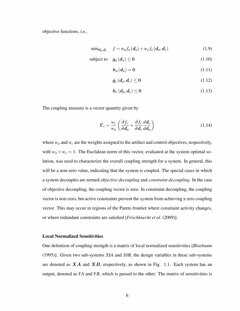
objective functions, i.e.,
minda,dc f = wa fa (da)+wc fc (da,dc) (1.9)
subject to ga (da)≤ 0 (1.10)
ha (da) = 0 (1.11)
gc (da,dc)≤ 0 (1.12)
hc (da,dc)≤ 0 (1.13)
The coupling measure is a vector quantity given by
Γv =wc
wa
(∂ fc
∂da+
∂ fc
∂dc
ddc
dda
)(1.14)
where wa and wc are the weights assigned to the artifact and control objectives, respectively,
with wa + wc = 1. The Euclidean norm of this vector, evaluated at the system optimal so-
lution, was used to characterize the overall coupling strength for a system. In general, this
will be a non-zero value, indicating that the system is coupled. The special cases in which
a system decouples are termed objective decoupling and constraint decoupling. In the case
of objective decoupling, the coupling vector is zero. In constraint decoupling, the coupling
vector is non-zero, but active constraints prevent the system from achieving a zero coupling
vector. This may occur in regions of the Pareto frontier where constraint activity changes,
or where redundant constraints are satisfied [Frischknecht et al. (2009)].
Local Normalized Sensitivities
One definition of coupling strength is a matrix of local normalized sensitivities [Bloebaum
(1995)]. Given two sub-systems SSA and SSB, the design variables in these sub-systems
are denoted as XA and XB, respectively, as shown in Fig. 1.1. Each system has an
output, denoted as YA and Y B, which is passed to the other. The matrix of sensitivities is
6

then computed as [Bloebaum (1995)]
∂YA∂XA
0
0∂Y B
∂XB
=
1 −∂YA∂Y B
−∂Y B∂YA
1
dYA
dXAdYA
dXBdY B
dXAdY B
dXB
(1.15)
which are then scaled using the relations
∂YA′
∂Y B=
Y BYA
∂YA∂Y B
(1.16)
∂Y B′
∂YA=
YAY B
∂Y B∂YA
(1.17)
where A′, B′ are the scaled outputs.
Figure 1.1: Subsystem Configuration (after [Bloebaum (1995)])
Note that, while the equations are presented here for only two sub-systems, this cou-
pling metric can be used in systems with more than two sub-systems. Furthermore, it is
applicable to problems with bi-directional coupling.
Coupling Matrix
Another metric used to quantify coupling is a matrix developed by Alyaqout and co-
workers, which incorporates optimality conditions into the global sensitivity equations
7

[Alyaqout et al. (2005)]. This matrix takes the form of
Γm =
∂F∂ f1
∂ f1
∂y11...
∂F∂ fN
∂ fN
∂y1N...
∂F∂ f1
∂ f1
∂yN1...
∂F∂ fN
∂ fN
∂yNN
T
dy11
dx1
dy11
dx2· · · dy11
dxN...
...dy1N
dx1
. . . dy1N
dxN...
...dyN1
dx1
. . . ...
......
dyNN
dx1· · · · · · dyNN
dxN
+
∑
Nj=1
∂F∂x j
dx j
dx1...
∑Nj=1
∂F∂x j
dx j
dxN
T
+
∑
Np=1 ∑
Nj=1
(∂F∂ fp
∂ fp
∂x j
dx j
dx1
)...
∑Np=1 ∑
Nj=1
(∂F∂ fp
∂ fp
∂x j
dx j
dxN
)
T
.
(1.18)
where N is the number of sub-systems present indexed as j = 1, . . . ,N, F is the overall sys-
tem objective, y jp are coupling variables, fp are the individual system objective functions
indexed as p = 1, . . . ,N, x j are the variables in the total problem, x j are local copies of
x j, and y jp are local copies of y jp [Alyaqout (2006), Alyaqout et al. (2005)]. An uncou-
pled system would be characterized, in this case, by a zero matrix. It is useful to note that
this formulation is extremely general; not only can it be used in the case of bi-directional
coupling, but it can be used with multiple sub-systems. Thus, it is applicable to design prob-
lems more general than co-design. The functional form of F is not specified. Therefore,
Γm is not limited to a simple linear combination of sub-system objectives. Furthermore,
this measure allows both ‘global’ and ‘local’ copies of variables, and lends itself to more
complex decomposition strategies.
8

1.4 Examples of Coupled Systems
The literature on coupled systems is extremely rich, and presents examples from di-
verse areas such as aeronautical structures, machine tools, automotive engineering, micro-
electrical mechanical systems (MEMS), mechanisms, and chemical processing [e.g., Kaji-
wara and Haftka (2000), Chen and Cheng (2006), Fathy et al. (2003), Carley et al. (2001),
Tilbury and Kota (1999), Wan et al. (2002), Shabde and Hoo (2008)]. Several broad areas
shall be discussed here. These areas are structural systems, robotics and mechatronics, and
MEMS.
1.4.1 Structural Systems with Active Control
Some of the first systems in which coupling was studied were in the field of aerospace
engineering. A typical example of this would be an aerospace structure subject to active
control. There may be a high cost associated with weight, particularly for a structure that
is to be flown or placed in orbit [Hale et al. (1985)]. Thus, specifications for these struc-
tures typically emphasize minimum weight, which results in a more flexible structure that
can be more difficult to control. It has, therefore, been recognized by many researchers
that a sequential optimization, in which the structure itself is first optimized and then the
optimal controller is designed for that structure, may not produce an optimal system. The
structure may be very light, but it could require an unacceptably large control effort. Heavy
control actuators may be necessary in order to meet other specifications such as displace-
ments, buckling, vibration, and stress [Khot and Abhyankar (1993), Maghami et al. (1996),
Messac (1998)].
Experimental and analytical studies have been carried out, demonstrating the potential
for both detrimental and advantageous interactions between a structure and its controller
(e.g., Haftka et al. (1986), Rao and Pan (1990)). The problem of simultaneous design of a
structure and its controller is made easier by the linear models typically used for the struc-
ture. However, it still presents significant challenges, as discussed by numerous researchers
9
[Ou and Kikuchi (1996), Kosut et al. (1990), Milman et al. (1991), Sobieszczanski-Sobieski
and Haftka (1997)]. Some of the issues addressed in the literature are the effect of coupling
on the stability of the control system, the large number of modes of vibration present, and
a variety of techniques that can be used to design a ‘controllable’ structure [Haftka (1990),
Onoda and Watanabe (1989)]. These techniques include locating the open-loop eigenval-
ues in ‘desirable’ areas of the complex plane and the use of the controllability Grammian
matrix, which shall be discussed further in Section 1.6, to place actuators.
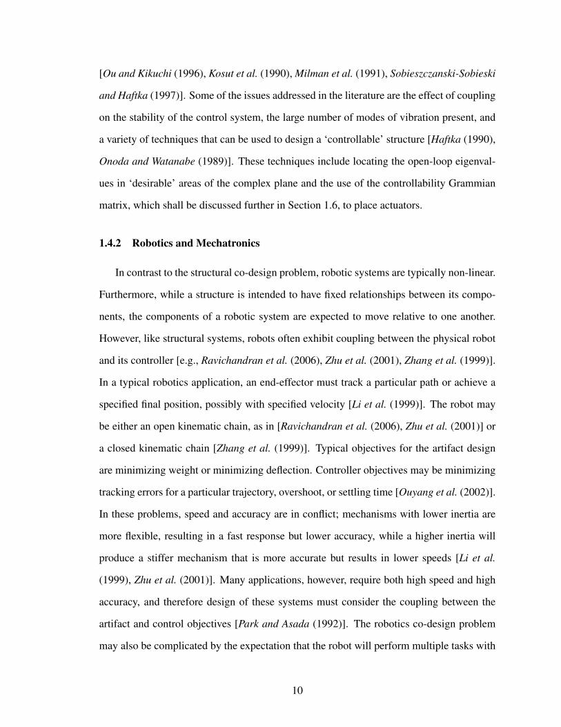
1.4.2 Robotics and Mechatronics
In contrast to the structural co-design problem, robotic systems are typically non-linear.
Furthermore, while a structure is intended to have fixed relationships between its compo-
nents, the components of a robotic system are expected to move relative to one another.
However, like structural systems, robots often exhibit coupling between the physical robot
and its controller [e.g., Ravichandran et al. (2006), Zhu et al. (2001), Zhang et al. (1999)].
In a typical robotics application, an end-effector must track a particular path or achieve a
specified final position, possibly with specified velocity [Li et al. (1999)]. The robot may
be either an open kinematic chain, as in [Ravichandran et al. (2006), Zhu et al. (2001)] or
a closed kinematic chain [Zhang et al. (1999)]. Typical objectives for the artifact design
are minimizing weight or minimizing deflection. Controller objectives may be minimizing
tracking errors for a particular trajectory, overshoot, or settling time [Ouyang et al. (2002)].
In these problems, speed and accuracy are in conflict; mechanisms with lower inertia are
more flexible, resulting in a fast response but lower accuracy, while a higher inertia will
produce a stiffer mechanism that is more accurate but results in lower speeds [Li et al.
(1999), Zhu et al. (2001)]. Many applications, however, require both high speed and high
accuracy, and therefore design of these systems must consider the coupling between the
artifact and control objectives [Park and Asada (1992)]. The robotics co-design problem
may also be complicated by the expectation that the robot will perform multiple tasks with
10

different specifications.
Robotics may be considered to be part of the field of mechatronics, an area which has
grown out of the union of mechanical and electrical systems. By its very nature, it re-
quires multidisciplinary optimization [Isermann (1996a), Isermann (1996b), Youcef-Toumi
(1996)]. Since it covers a wide range of applications, it is not possible to specify typ-
ical objectives for artifact and control design. There is a number of case studies in the
literature, showing that, in at least some cases, the artifact and control designs are cou-
pled. These cases include machine tools, automotive suspensions, and elevators [Chen and
Cheng (2005), Fathy et al. (2003), Fathy et al. (2002)].
Because of the non-linear nature of many of these problems, techniques that have been
successfully used in structural applications are not generally applicable. In addition, the
specifications and constraints are typically different than those in structural co-design prob-
lems. In the design of aerospace structures, the size of actuators is typically subject to
restrictive limits. In robotics and mechatronics, the actuators are still limited in size, but
accuracy is weighted more heavily in the overall system performance. Many of the meth-
ods used for co-design in robotics and mechatronics are based on either experimentation,
as in [Pil and Asada (1996)], or on heuristics, as in [Li et al. (2001)].
1.4.3 MEMS
Yet another area in which the artifact and control design problems can be coupled is
the field of microelectrical mechanical systems (MEMS). MEMS devices are typically
made of silicon, or a silicon-based polymer such as polydimethyl siloxane (PDMS), with
their mechanical and electrical components integrated as they are created on a silicon
wafer. These devices may be used in applications such as positioning of mirrors in op-
tical switches, magnetic storage devices, acceleration sensors, and gyroscopes, to name a
few [Chu et al. (2005), Carley et al. (2001), Oldham et al. (2005), Wolfram et al. (2005),
Park and Horowitz (2003)]. The MEMS device typically must be designed to have a certain
11

range of motion for an actuator or sensing range for a sensor, with a controller designed to
give a fast response and high accuracy. These objectives are often conflicting. In addition,
MEMS devices may experience an instability problem known as pull-in. In this condition,
for higher voltages, there is no stable position for the device. The voltage at which this
occurs is a function of the physical configuration of the device, and therefore couples the
artifact design and control design problems. This phenomenon has been a subject of con-
cern in many devices, including comb drives [Legtenberg et al. (1996)] and microbeams
[Abdalla et al. (2005)].
1.5 Optimization Methods for Coupled Systems
While some systems are weakly coupled or uncoupled, many systems do exhibit strong
coupling. In particular, it has been shown that both uncertainty in system parameters and
more demanding performance requirements are associated with strongly coupled systems
[Youcef-Toumi (1996)]. Similarly, uncertainty and increased performance requirements are
associated with coupling in the related problem of modeling and controller design [Brusher
et al. (1997a), Brusher et al. (1997b)]. The demonstrated existence of coupled systems, and
their prevalence, quite naturally leads to the question of how to design such systems most
effectively. A number of strategies have been developed, both sequential and simultaneous,
as shown in Fig. 1.2 [Fathy (2003)].
1.5.1 Sequential Optimization
The sequential approach is the traditional practical means of optimizing co-design prob-
lems. In the simplest sequential strategy, the artifact is first optimized. In the case of
uni-directional coupling, the controller architecture is completely ignored. If bi-directional
coupling exists, then the control design variables are assumed to take on certain values,
which are parameters in the initial optimization. Once this design is complete, the artifact
design variables are treated as parameters in the design of the controller. This approach
12

Figure 1.2: Solution Methods for Coupled Systems (after [Fathy (2003)])
works well in many cases. However, it will only find the system optimum when coupling
does not exist. When uni-directional coupling is present, the solution found will be optimal
for the artifact objective, fa, but not for the control objective, fc. In fact, it may prove
to be impossible to find a feasible solution for the controller design. In the case of bi-
directional coupling, the solution found may not be optimal for either objective function.
This method of solution does not provide the designer with any information on the nature
of tradeoffs present between the artifact and controller objectives, and thus even in the case
of uni-directional coupling, where the solution lies at an endpoint of the Pareto frontier, the
designer is unable to consider the merits of different designs on the Pareto frontier.
Because of the disadvantages of a simple sequential optimization, a modified sequential
formulation has been utilized for a number of systems. This strategy includes one or more
constraints on the artifact design that are intended to predispose the resultant design to
effective control and ensure that a feasible control design will exist. The most commonly
13

used constraint is based on open-loop eigenvalues. In the design of the artifact, the system’s
open-loop eigenvalues are required to fall into a certain region of the complex plane. This
method is typically used in structural applications, and in certain cases it can be quite
effective. The combined artifact and control problem can be formulated to use this type
of approach to avoid areas of high sensitivity and move the eigenvalues into acceptable
regions when the structure is designed, thus predisposing the structure to effective control
[Bodden and Junkins (1985)]. These methods are not always applicable, however, and they
can also present some difficulties. The problem can become of very high dimensionality
due to the large number of structural vibration modes and is often non-linear [Bodden and
Junkins (1985)]. Some difficulties with this approach were overcome by Yee and Tsuei,
who developed a more efficient method of effectively locating the eigenvalues [Yee and
Tsuei (1991)]. This method, however, locates the open-loop eigenvalues, while the system
behavior is controlled by the closed-loop eigenvalues. The literature has shown that in some
cases, the locations of the closed-loop eigenvalues will not fall into acceptable regions when
this approach is used [Belvin and Park (1990), Eastep et al. (1987)]. At this point, there is
no sequential method of design that effectively locates closed-loop eigenvalues.
As previously stated, methods of design that may be effective for structural applications,
such as the location of open-loop eigenvalues, are typically not applicable to non-linear
problems such as robotics and mechatronics, and researchers have developed methods with
these types of problems in mind. One method of modifying the design problem in order to
account for coupling, specifically intended for mechatronic applications, is described in [Li
et al. (2001)]. It emphasizes finding a simple dynamic model of the system of interest and
the selection of parameters in the artifact design problem in order to facilitate control. Since
mechatronic applications have not typically been given any kind of a standard formulation,
there is a great deal of variety in the design problems that could arise, and the method
described is quite general in nature.
14

1.5.2 Iterative Optimization
In this approach, the system is repeatedly solved, first for the artifact design, then for
the controller design. The solution from each iteration becomes the starting point for the
new iteration [Grigoriadis and Skelton (1998)]. One advantage of this approach is that it
maintains the smaller sub-problems of the sequential optimization. It does converge to a
solution in some cases, but not in others, and it cannot be guaranteed to converge to an
optimal solution [Reyer (2000)].
1.5.3 Simultaneous Optimization
In simultaneous optimization, an overall system objective is defined as a function of
the individual sub-system objective functions, fa and fc. Typically, this is a linear com-
bination. However, due to the inherent limitations of this type of system objective, such
as the inability to find points on a non-convex Pareto frontier, other formulations may be
used [Athan (1994), Athan and Papalambros (1996), Das and Dennis (1997)]. The con-
straints and design variables for the simultaneous problem are the union of the individual
constraints and variables for the individual sub-problems. Thus, the problem is formulated
as in Eqs. (1.19) - (1.23).
minda,dc f = f ( fa (da,dc) , fc (da,dc)) (1.19)
subject to ga (da,dc)≤ 0 (1.20)
gc (da,dc)≤ 0 (1.21)
ha (da,dc) = 0 (1.22)
hc (da,dc) = 0 (1.23)
This approach has the advantage that, if a solution is found, it will be system optimal. How-
ever, this approach has some disadvantages. It may be operationally inconvenient, since the
problem requires two disparate objectives from different disciplines to be formulated and
15
combined. The problem cannot be solved until both the artifact and control objectives have
been formulated, so it requires the choice of controller architecture to be made early in
the design process, prior to the final design of the artifact. The simultaneous problem is
also computationally intensive due to its larger size, and may be non-convex, even if the
individual objectives fa and fc are convex [Balling and Sobieszczanski-Sobieski (1996)].
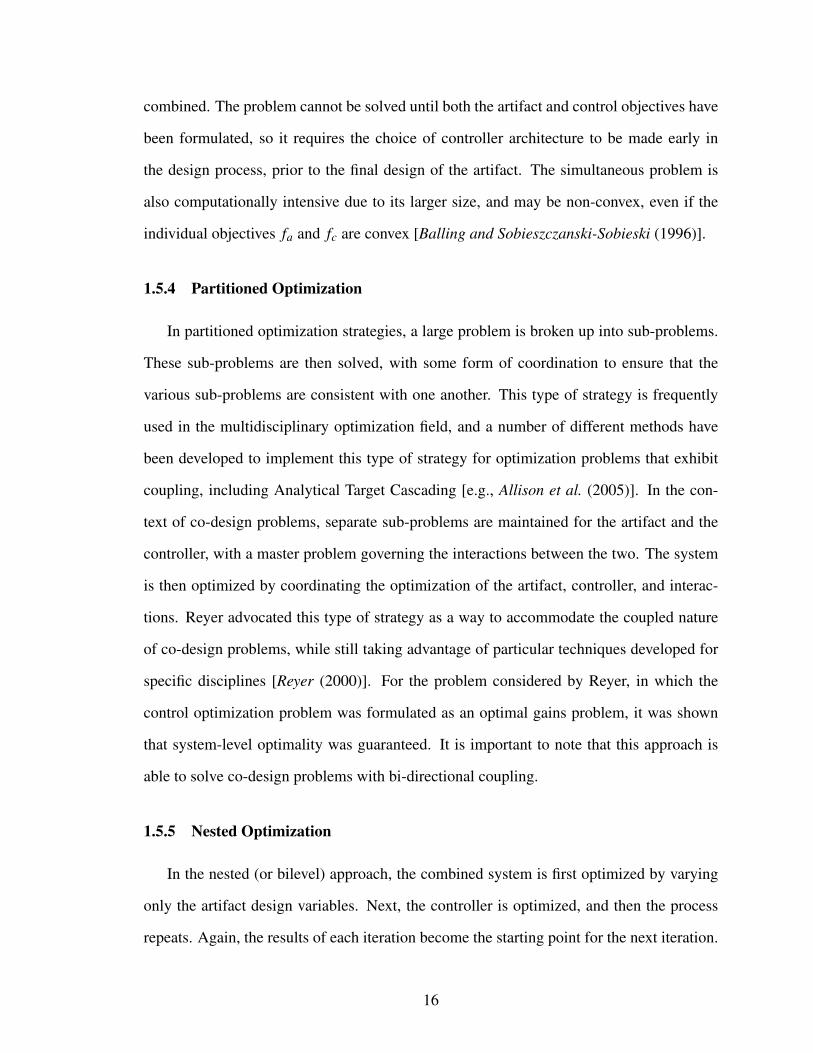
1.5.4 Partitioned Optimization
In partitioned optimization strategies, a large problem is broken up into sub-problems.
These sub-problems are then solved, with some form of coordination to ensure that the
various sub-problems are consistent with one another. This type of strategy is frequently
used in the multidisciplinary optimization field, and a number of different methods have
been developed to implement this type of strategy for optimization problems that exhibit
coupling, including Analytical Target Cascading [e.g., Allison et al. (2005)]. In the con-
text of co-design problems, separate sub-problems are maintained for the artifact and the
controller, with a master problem governing the interactions between the two. The system
is then optimized by coordinating the optimization of the artifact, controller, and interac-
tions. Reyer advocated this type of strategy as a way to accommodate the coupled nature
of co-design problems, while still taking advantage of particular techniques developed for
specific disciplines [Reyer (2000)]. For the problem considered by Reyer, in which the
control optimization problem was formulated as an optimal gains problem, it was shown
that system-level optimality was guaranteed. It is important to note that this approach is
able to solve co-design problems with bi-directional coupling.
1.5.5 Nested Optimization
In the nested (or bilevel) approach, the combined system is first optimized by varying
only the artifact design variables. Next, the controller is optimized, and then the process
repeats. Again, the results of each iteration become the starting point for the next iteration.
16

It has been shown that, in the case of uni-directional coupling, this approach will yield
system-optimal solutions [Fathy (2003)], but in bi-directional coupling it may not [Reyer
(2000)].
1.6 Use of Controllability in System Design
As discussed in Sections 1.4.1 and 1.5.1, open-loop eigenvalues have been used as a
measure of a system’s ‘ease of control’. In addition to these efforts, other control charac-
teristics have been used in system design, particularly to locate actuators and sensors [Roh
and Park (1997), Lim and Gawronski (1993), Junkins and Kim (1993)]. In these efforts,
researchers have considered how to link the concepts of controllability and observability to
the output of a physical system [e.g., Muller and Weber (1972), Brown (1966)]. Muller and
Weber examined this issue in detail, considering several candidates for physically mean-
ingful metrics based on the inverse of the controllability Grammian matrix, W−1c(t f),
where t f is the final time of the interval of interest. Their candidates were the maximum
eigenvalue of W−1c(t f), the trace of W−1
c(t f), and the determinant of W−1
c(t f). Their
analysis indicated that any of these three measures could be used to formulate some ‘mea-
sure of quality’ of a time-varying system [Muller and Weber (1972)]. Furthermore, they
showed that optimization of a system using such a measure can produce a system that is
amenable to control. This dissertation will make use of this concept in the development of
the Control Proxy Function (CPF) problem formulation in Chapter IV, with several CPFs
based on the controllability Grammian matrix, which is further discussed in Section 3.2.
1.7 Original Contributions
This chapter introduced the co-design problem, described the ways in which coupling
can be measured in this type of problem, and presented some examples from the literature
demonstrating the existence of coupling. It also presented a brief survey of the optimiza-
17

tion methods available to solve the co-design problem. Despite the depth and breadth of
previous work in this area, there are still important unanswered questions and issues that
have not yet been resolved. This dissertation answers some of these questions. Specifically,
it makes the following original contributions:
1. Derivation of relationships between coupling measures, with the extension of the
coupling vector to bi-directional cases
The existence of multiple coupling measures quite naturally raises the question of
how they might relate to one another. Since these various measures allegedly are
measuring the same thing, one might expect that there will be some relationship
between them. This dissertation shows that there are indeed relationships between
different coupling measures. Furthermore, in the case of one coupling measure, the
coupling vector Γv, it is possible to extend the range of application of the measure,
from uni-directional coupling only to also include bi-directional coupling, and this is
also presented.
2. Derivation of relationships between coupling and controllability for several important
classical control problems
One weakness of the currently used coupling measures is the need to evaluate them at
an optimal solution. In other words, the co-design problem must first be solved before
the strength of the coupling can be determined with certainty. However, knowing
the strength of the coupling prior to attempting a solution would be desirable, since
that information could be used in the selection of a method of solution. In several
important classical control problems, it is possible to obtain an expression for the
coupling vector, Γv, that is independent of the controller architecture. Thus, it is
possible to study the coupling prior to solving the co-design problem. There are
several conditions under which coupling can be shown to vanish, prior to the problem
solution, and these conditions are discussed.
18

3. Development of a modified sequential method using a Control Proxy Function (CPF)
for cases of uni-directional coupling
As discussed in Section 1.5.1, there have been a number of attempts to design a
system for ‘ease of control’. This dissertation introduces a particular formulation
of the co-design problem, using a Control Proxy Function (CPF), to predispose the
artifact to ease of control. Guidelines are given for the choice of an effective CPF,
a condition to guarantee Pareto optimality is presented, and a measure of the quality
of the CPF solution is derived. It is important to note that this quality measure,
which indicates the ‘distance’ from Pareto optimality, can be evaluated without any
information about the true Pareto frontier.
4. Categorization of problems according to the nature of coupling and appropriate solution
methods
As discussed in Section 1.5, there is a variety of solution methods available. Choice
of an appropriate method is critical in the efficient and effective solution of a co-
design problem. Guidelines are presented for the categorization of co-design prob-
lems based on the existence and nature of the coupling (bi-directional, uni-directional,
or uncoupled), and appropriate solution methods are indicated for each case. These
guidelines include the evaluation of whether the new CPF method is suitable for a
given problem, and if it is, what type of CPF should be selected.
5. Application of new method to case studies
A co-design problem is formulated using a MEMS actuator, and solved with the new
CPF method. Two different problem formulations are presented, and it is shown that
in each case, an appropriate CPF can be chosen which yields Pareto optimal results.
19

1.8 Dissertation Outline
The following chapters describe the above contributions in further detail. Chapter II
shows the relationships between the coupling vector, Γv, and each of the other coupling
metrics presented in Section 1.3.2. It also shows the relationship between Γv and the slope
of the Pareto frontier, and extends the range of applicability of Γv to problems in which the
system objective function is a non-linear combination of fa and fc, and to problems that
exhibit bi-directional coupling. Chapter III presents the relationships between coupling, as
measured by Γv, and the controllability Grammian matrix, Wc. The relationship between
Γv and Wc(t f)
is derived for two classical control problems, that of minimizing control
effort and that of minimizing time subject to a constraint on control effort. In addition,
a relationship between Γv and the steady-state controllability Grammian, W∞c , is derived
for Linear Quadratic Regulator (LQR) control. In Chapter IV, the Control Proxy Function
(CPF) method is formulated for problems with uni-directional coupling. The characteristics
of an effective CPF are given, and a metric is provided for the evaluation of a CPF. The
given conditions are then used to derive several CPFs that are effective for specific problem
formulations. In Chapter V, a method is presented for the evaluation of co-design problems
to determine the nature of coupling and to choose an appropriate solution method. This
method is then demonstrated through the solution of two co-design problems for a MEMS
actuator. The thesis concludes in Chapter VI with a summary, concluding remarks, and
discussion of future work.
The appendices provide additional details on the proofs of certain theorems (Appendix
A) and the optimization model formulation used in Chapter V (Appendix B).
20

CHAPTER II
Relationships Between Coupling Measures
2.1 Introduction
As discussed in Section 1.3.2, there are several measures of coupling proposed in the
literature. This raises questions about whether these metrics are measuring the same quan-
tity, how they may be related, and how to choose among them in a given problem. In this
chapter, it will be shown that various measures of coupling are related. However, they are
not equivalent, and they are not necessarily commensurate. This will be illustrated with a
simple example. One of these measures, the coupling vector Γv, is specifically chosen for
use in this work. Its physical interpretation shall be addressed, and extensions to its range
of applicability will be derived.
2.2 Relations between Coupling Measures
In this section, relationships will be derived between the coupling vector, Γv, and each
of three other coupling measures. These three coupling vectors are the sensitivity of the
control objective, normalized sensitivities, and the coupling matrix, Γm. It will be shown
that the coupling vector and the sensitivity of the control objective are commensurate, while
the coupling vector is not commensurate with either the normalized sensitivities or the
coupling matrix, Γm.
21

2.2.1 Coupling Vector, Γv, and Sensitivity of the Control Objective
Consider a co-design problem with uni-directional coupling that takes the form of Eqs.
(2.1) - (2.3).
minda,dc
fa (da)+wc
wafc (da,dc) (2.1)
subject to ga (da)≤ 0 (2.2)
wc
wagc (da,dc)≤ 0 (2.3)
The Karush-Kuhn-Tucker (KKT) conditions [Papalambros and Wilde (2000), Kuhn and
Tucker (1950)] may be written as
[∂ fa
∂da+
wc
wa
∂ fc
∂da
wc
wa
∂ fc
∂dc
]−[µ1 µ2
] ∂ga
∂da0
wc
wa
∂gc
∂da
wc
wa
∂gc
∂dc
= 0 (2.4)
The vector Γv was defined in [Fathy (2003)] as the difference between the KKT conditions
for a coupled and uncoupled system, and is found to be
Γv =wc
wa
(∂ fc
∂da−µ2
∂gc
∂da
)(2.5)
evaluated at the system optimum, which can then be written in terms of the sensitivity
metric introduced in Section 1.3.2 as
Γv =wc
wa
∂ f ∗c∂da
. (2.6)
Therefore, Γv will be parallel to∂ f ∗c∂da
. These two measures will be consistent in determining
whether or not a system is coupled, and in determining which of two systems is more
strongly coupled.
22

2.2.2 Coupling Vector, Γv, and Coupling Matrix, Γm
As noted in Section 1.3.2, the coupling vector Γv and coupling matrix Γm do not have
the same range of applicability. Therefore, in order to examine the relationship between
the two coupling measures, certain assumptions are necessary.
1. The system has two objective functions, one for the artifact and one for the controller.
2. Coupling is unidirectional.
3. The overall objective function is a weighted sum of the individual objectives.
4. There are no local copies of variables.
The system in question, then, can be represented by the diagram given in Fig. 2.1.
From assumptions 1–4, the following substitutions can be made in Eq. (1.18):
N = 2
f1 = fa
f2 = fc
x1 = x1 = 0
x2 = x2 = dc
y12 = y12 = da
y21 = y21 = da
y11 = y11 = 0
y22 = y22 = 0
These substitutions give a simplified coupling matrix
Γm =
0
wa∂ fa
∂da
dda
ddc+wc
∂ fc
∂da
dda
ddc+wc
∂ fc
∂dc
T
. (2.7)
23

Figure 2.1: Subsystem Structure for Simplified System
It is then possible to relate Γv and Γm:
Γm =
0
wa
(d fa
ddc+(
Γv−wc
wa
∂ fc
∂dc
ddc
dda
)dda
ddc+
wc
wa
∂ fc
∂dc
)
T
. (2.8)
If the problem is unconstrained, then Eq.( 2.8) simplifies to
Γm =
0
wad fa
ddc+waΓv
dda
ddc
T
. (2.9)
The derivative ddaddc
can be calculated either analytically, from the KKT conditions, or nu-
merically.
The following observations can then be made:
1. Γm captures information about the interactions between variables in each sub-problem
that is not contained within Γv. This is consistent with the differing origins of the
metrics. Since Γm was derived from the GSEs, it can be expected to contain infor-
mation about the sensitivity of one variable to another within the same sub-system.
2. In a problem with active constraints, it is possible for Γm to be non-zero when Γv = 0.
This would indicate that relations between the design variables in a sub-system are
highly significant, and the solution will be sensitive to small changes in the variables.
3. In both a constrained and an unconstrained problem, it is possible for Γm and Γv to
24

disagree on when a system is more strongly coupled. This will happen in the case of
high sensitivity in the relations between the variables.
4. For the case where constraints are active, but there is only one artifact design variable
and one controller design variable, Eq.(2.8) simplifies to Eq.(2.9), just as it does for
the unconstrained case. This reflects the fact that there are no possible interactions
between variables within a sub-system. The same situation will occur when all active
constraints consist of simple bounds.
5. If an unconstrained system is uncoupled, then fa = fa(da) and fc = fc(dc). In this
case,d fa
ddc= 0 since, by definition of an uncoupled system, the artifact objective
function fa does not depend on the controller variables dc. Also, Γv = 0, since the
equations representing the KKT conditions will be identical for both sequential and
simultaneous solutions of the system. This results in Γm = 0, and therefore the two
criteria will be consistent in having zero value for uncoupled problems.
2.2.3 Coupling Vector, Γv, and Normalized Sensitivities
In evaluating the application of normalized sensitivities
∂ fa
∂da0
0∂ fc
∂dc
=
1 −∂ fa
∂ fc
−∂ fc
∂ fa1
d fa
dda
d fa
ddcd fc
dda
d fc
ddc
(2.10)
The coupling vector, Γv, can be expressed as
Γv =wc
wa
d f ∗cdda
(2.11)
25

and thus Eq. (2.10) can be seen to contain Γv, as shown below.
∂ fa
∂da0
0∂ fc
∂dc
=
1 −∂ fa
∂ fc
−∂ fc
∂ fa1
d fa
dda
d fa
ddcwa
wcΓv
d fc
ddc
(2.12)
These metrics are not commensurate, since the normalized sensitivities contain terms that
do not appear in Γv.
2.3 Illustrative Example: Positioning Gantry
In this section, the coupling vector and coupling matrix are applied to a simple system,
and it is shown that they agree on the presence of coupling in some cases and disagree in
others. The system shown here shall be used also as an illustrative example in Chapter III.
Figure 2.2: Configuration of Positioning Gantry
Consider a simple model of a positioning gantry, as shown in Fig. 2.2. In this system,
a mass M is connected to a fixed surface by a linear spring with constant ks. A flexible
26

Figure 2.3: Schematic of System Controller
inelastic belt is connected to the mass and wraps around a pulley with radius r, which is
mounted on a DC motor with armature resistance Ra and motor constant kt . It is assumed
that the rotor inertia of the motor and the inertia of the pulley are negligible. The motor will
be actuated by a voltage signal. The displacement of the mass from its original position is
Z. The system can be modeled by the following equations:
x = Ax+Bu (2.13)
Z = Cx (2.14)
x =
Z
Z
(2.15)
A =
0 1
− km− b
m
(2.16)
B =
01m
(2.17)
C =[
1 0
](2.18)
27

where u is the voltage, V , and the terms m, b, and k are given by
m =MrRa
kt(2.19)
b =kt
r(2.20)
k =ksrRa
kt(2.21)
A state-feedback controller with a precompensator G and gainsK = [K1 K2] is applied
to the system, as shown in Fig. 2.3. This system will be optimized twice. The artifact
objective function fa will remain the same, but the artifact design variables da and artifact
constraint g1 will be changed to produce both an uncoupled and a coupled optimization
problem. The artifact objective is to maximize the steady-state displacement of the mass,
Zss. The controller objective function fc, controller design variables dc, and controller con-
straint g2 take the same form in both formulations. The controller objective is to minimize a
combination of the maximum voltage Vmax and the settling time ts. The relative importance
of Vmax and ts are specified by weighting parameters.
2.3.1 Uncoupled System Optimization
The system optimization formulation is:
minr,kt ,K1,K2,G
wa fa +wc fc (2.22)
subject to g1 = c1 +(
ktVss
rRa− c2
) 12
− r ≤ 0 (2.23)
g2 = Mp−Mp,all ≤ 0 (2.24)
h1 = Zss−Zr = 0 (2.25)
28
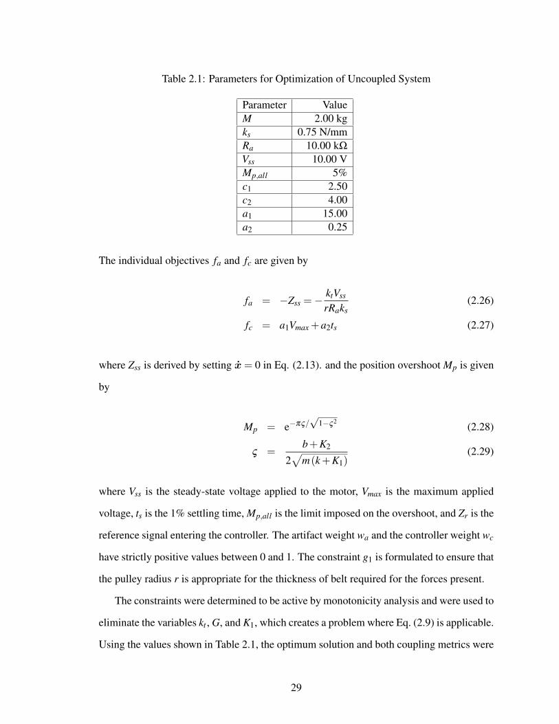
Table 2.1: Parameters for Optimization of Uncoupled System
Parameter ValueM 2.00 kgks 0.75 N/mmRa 10.00 kΩ
Vss 10.00 VMp,all 5%c1 2.50c2 4.00a1 15.00a2 0.25
The individual objectives fa and fc are given by
fa = −Zss =− ktVss
rRaks(2.26)
fc = a1Vmax +a2ts (2.27)
where Zss is derived by setting x= 0 in Eq. (2.13). and the position overshoot Mp is given
by
Mp = e−πς/√
1−ς2(2.28)
ς =b+K2
2√
m(k +K1)(2.29)
where Vss is the steady-state voltage applied to the motor, Vmax is the maximum applied
voltage, ts is the 1% settling time, Mp,all is the limit imposed on the overshoot, and Zr is the
reference signal entering the controller. The artifact weight wa and the controller weight wc
have strictly positive values between 0 and 1. The constraint g1 is formulated to ensure that
the pulley radius r is appropriate for the thickness of belt required for the forces present.
The constraints were determined to be active by monotonicity analysis and were used to
eliminate the variables kt , G, and K1, which creates a problem where Eq. (2.9) is applicable.
Using the values shown in Table 2.1, the optimum solution and both coupling metrics were
29

Table 2.2: Results of Optimization of Uncoupled System
Quantity Value
da =[
rkt
] [2.50 cm
10.00 N-m/A
]dc =
K1K2G
0.721.232.59
Zss 5.33 cmts 8.79 sVmax 13.83 V
calculated. The optimal values of the design variables and of Zss, Vmax, and ts are given
in Table 2.2. For all values of wa and wc in the specified range, Γv = 0 and Γm = [0 0],
and, therefore, both measures were consistent in indicating that the system is uncoupled.
These coupling measures are also consistent with the results of the system optimization
itself; identical results were found for both sequential optimization and for simultaneous
optimization with various combinations of weights.
This co-design problem can be solved without eliminating constraints, however. Con-
sider the case where the variables kt and K1 are retained, but the variable G is eliminated
by substitution. In this case, the coupling vector, Γv, is given by the relation
Γv =wc
wa
∂ fc
∂ r∂ fc
∂kt
T
+
∂ fc
∂K1∂ fc
∂K2
T ∂K1
∂ r∂K1
∂kt∂K2
∂ r∂K2
∂kt
(2.30)
The problem is still uncoupled, as determined by Γv; at the solution,
Γv =[
0 0
]. (2.31)
However, the problem is not uncoupled when the coupling matrix, Γm, is used. For this
30

form of the problem,
Γm =
0
wa
∂ fa
∂ r∂ fa
∂kt
T ∂ r
∂K1
∂ r∂K2
∂kt
∂K1
∂kt
∂K2
+wc
∂ fc
∂ r∂ fc
∂kt
T ∂ r
∂K1
∂ r∂K2
∂kt
∂K1
∂kt
∂K2
+
∂ fc
∂K1∂ fc
∂K2
T
.
(2.32)
For the weights wa = 0.5, wc = 0.5, the matrix Γm is computed as
Γm =
0 0
−0.162 −0.183
(2.33)
Note, then, that if constraints are active, Γv and Γm may disagree on whether or not a prob-
lem is coupled. Furthermore, Γm can indicate that the same problem is either coupled or
uncoupled, depending on the formulation of that problem. This indicates that, if parametric
uncertainty in the constraints is neglected, the problem will be uncoupled; however, Γm is
capable of capturing information on the parametric uncertainty of the constraints, and this
uncertainty will affect the control objective of the co-design problem [Alyaqout (2006)].
2.3.2 Coupled System Optimization
Now, consider a different formulation of the system optimization. In this case, the
design variables are ks, Ra, G, K1, and K2, the objective functions and constraints g2 and h1
are unchanged, but constraint g1 is changed. The new constraint g1 is formulated to ensure
that the spring is sized appropriately for the loads present.
31
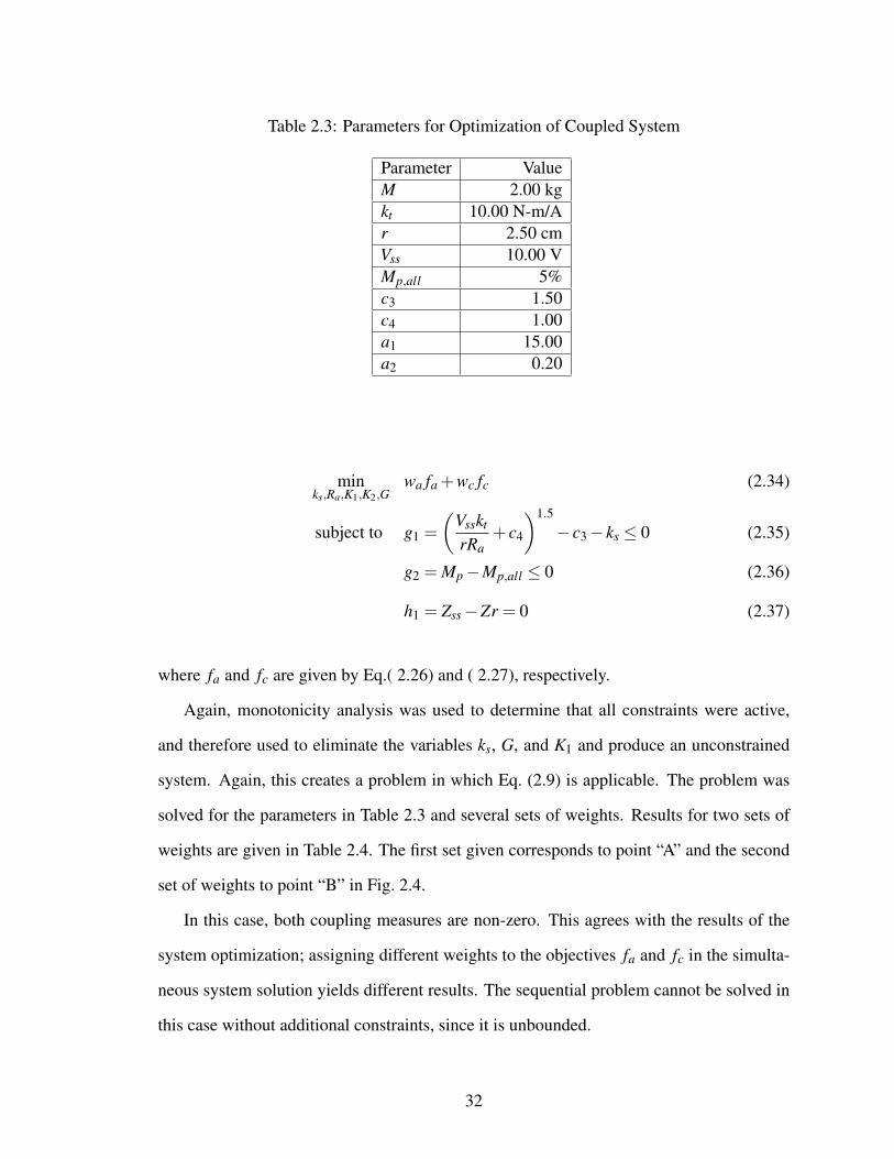
Table 2.3: Parameters for Optimization of Coupled System
Parameter ValueM 2.00 kgkt 10.00 N-m/Ar 2.50 cmVss 10.00 VMp,all 5%c3 1.50c4 1.00a1 15.00a2 0.20
minks,Ra,K1,K2,G
wa fa +wc fc (2.34)
subject to g1 =(
Vsskt
rRa+ c4
)1.5
− c3− ks ≤ 0 (2.35)
g2 = Mp−Mp,all ≤ 0 (2.36)
h1 = Zss−Zr = 0 (2.37)
where fa and fc are given by Eq.( 2.26) and ( 2.27), respectively.
Again, monotonicity analysis was used to determine that all constraints were active,
and therefore used to eliminate the variables ks, G, and K1 and produce an unconstrained
system. Again, this creates a problem in which Eq. (2.9) is applicable. The problem was
solved for the parameters in Table 2.3 and several sets of weights. Results for two sets of
weights are given in Table 2.4. The first set given corresponds to point “A” and the second
set of weights to point “B” in Fig. 2.4.
In this case, both coupling measures are non-zero. This agrees with the results of the
system optimization; assigning different weights to the objectives fa and fc in the simulta-
neous system solution yields different results. The sequential problem cannot be solved in
this case without additional constraints, since it is unbounded.
32

Table 2.4: Results of Optimization of Coupled System
Value for Given WeightsPoint A Point B
Quantity wa = 0.4, wc = 0.6 wa = 0.7, wc = 0.3
da =[
Raks
] [28.60 kΩ
2.21 N/mm
] [38.75 kΩ
1.40 N/mm
]dc =
K1K2G
−1.4315.8114.40
−2.1516.5011.38
Zss 0.63 cm 0.74 cmts 6.64 s 8.70 sVmax 10.26 V 10.27 VΓv 0.058 0.113
Γm
[0
0.0039
]T [0
−0.0033
]T
Figure 2.4: Pareto Points for Coupled System Optimization
33
Note that, while both coupling metrics agree that the system is coupled, they do not
agree on the coupling strength. The value of Γv is positive for both points considered, but
the non-zero component of Γm experiences a sign change between points A and B. The two
measures are clearly not commensurate, even when they agree on the existence of coupling.
2.4 Choice of Coupling Metric
It has been shown that, of the four coupling metrics considered, only two of them are
commensurate. The coupling vector, Γv, is commensurate with the sensitivity of the control
objective. However, the coupling vector is not commensurate with either the coupling
matrix, Γm, or with the normalized sensitivities. Therefore, it is necessary to consider
which of these measures is most appropriate for this work. In this thesis, the coupling
vector, Γv, is chosen to represent coupling. This measure is judged to be most appropriate
due to its simpler form and applicability to the problems of interest, i.e., co-design problems
with uni-directional coupling.
2.5 Physical Significance of Coupling Vector
While the coupling vector, Γv, is derived from the KKT conditions, it also has a physical
interpretation as a component of the slope of the Pareto frontier for a co-design problem
that exhibits uni-directional coupling. For the coupled co-design problem described here,
it is possible to describe the relation between the optimum values of the two objectives as
follows:
f ∗c = f ( f ∗a ) (2.38)
By differentiating Eq. ( 2.38) and making appropriate substitutions, the slope of the Pareto
frontier can be expressed asd f ∗cd f ∗a
=wa
wcΓv
dda
d fa
∗. (2.39)
34

The physical significance of the coupling vector Γv, therefore, is that it contributes to the
slope of the Pareto frontier, leading to the following observations:
1. If the coupling vector vanishes at one particular point, then the Pareto frontier will
have zero slope at that point. If this point is not an end point of the Pareto frontier,
then the curve will either be non-convex or discontinuous at this point.
2. It is possible for a non-zero coupling vector to be present at a point of zero slope. In
this case, the coupling vector would be orthogonal to the derivativedda
d fa
∗.
3. Large changes in the direction of the coupling vector, while not definitive, may be a
warning sign of a non-convex or discontinuous Pareto frontier, particularly when the
derivative vectordda
d fa
∗does not experience similar changes in its direction.
Information about the nature of the Pareto frontier can be useful. As noted in Section
1.5.3, if the Pareto frontier is determined to be non-convex, then a linear combination of
objectives is not an effective formulation and another formulation, such as an exponential
weighted criteria function [Athan (1994)], will be required. If the Pareto frontier is both
convex and continuous, then it could be approximated by fitting a convex continuous curve
to a relatively small number of points. This can be useful when the designer wishes to
find points in a particular area of the Pareto frontier. Methods do exist for finding points
in specific areas of the Pareto frontier, such as the normal-boundary intersection method
to find the “knee” [Das (1999)]. However, the ability to approximate the curve is useful
when another area of the Pareto frontier is considered to be desirable. Determination of
the approximate curve has the potential to reduce the computational requirements to solve
a problem.
2.6 Extensions of Coupling Vector, Γv
As stated in Section 1.3, the coupling vector, Γv, was derived based on certain as-
sumptions. These assumptions impose limitations on the types of problems for which it is
35
applicable. Here, it will be shown that the scope of Γv may be extended in two ways. One
extension, to problems in which the objective function is not a linear combination of fa and
fc, will be directly relevant to this dissertation. The second extension, to problems with
bi-directional coupling, will not be used for this work. However, it may be useful for later
extension of this work to co-design problems with bi-directional coupling.
2.6.1 Extension of Coupling Vector to Non-Linear Objective Combination
Assume that a co-design problem is formulated as the sum of two functions, F1 and F2,
as in Eqs. (2.40) - (2.44). The functions F1 ( fa) and F2 ( fc) are any functions that satisfy
the conditions given in Eqs. (2.45) - (2.46).
minda,dc
F = F1 ( fa (da))+F2 ( fc (da,dc)) (2.40)
subject to ga (da)≤ 0 (2.41)
ha (da) = 0 (2.42)
gc (da,dc)≤ 0 (2.43)
hc (da,dc) = 0 (2.44)
argmin(F1 ( fa (da))) = argmin( fa (da)) (2.45)
argmin(F2 ( fc (da,dc))) = argmin( fc (da,dc)) (2.46)
Furthermore, assume that the control design variables, dc, can be expressed as a function
of the artifact design variables, da, i.e., dc = dc (da). Then, the KKT conditions can be
36

written as ∂ fa
∂da+
∂F2∂ fc∂F1∂ fa
(∂ fc
∂da+
∂ fc
∂dc
dc
∂da
)∂F2∂ fc∂F1∂ fa
∂ fc
∂dc
+λT
∂ha
∂da∂hc
∂dc
+µT
∂ga
∂da∂gc
∂dc
= 0(2.47)
µT
ga (da)
gc (da,dc)
= 0 (2.48)
λ 6= 0 (2.49)
µ≥ 0 (2.50)
It is then possible to equate a generalized coupling vector, Γ′v, with the difference between
the KKT conditions for the coupled and the uncoupled problem.
Γ′v =
∂F2/∂ fc
∂Fa/∂ fa
(∂ fc
∂da+
∂ fc
∂dc
∂dc
∂da
)(2.51)
Note that the vector Γ′v is parallel to the vector Γv. Therefore, any statement based on the
direction of Γv will also apply to Γ′v. The original coupling vector Γv is a special case of
Γ′v, where F1 ( fa) = wa fa and F2 ( fc) = wc fc. Note that Γ′
v is not valid if a non-separable
function of both fa and fc is considered.
As an example of a non-linear combination of fa and fc, consider the exponential
weighted criteria formulation [Athan (1994)]. This formulation is given by
f = (enwa−1)e fa +(enwc−1)e fc (2.52)
where n is a parameter, and wa and wc are the relative weights of fa and fc. For this
formulation,
Γ′v =
(enwc−1)e fc
(enwa−1)e fa
(∂ fc
∂da+
∂ fc
∂dc
∂dc
∂da
)(2.53)
37

Since Γ′v ‖Γv, any derivations based on the direction of Γv will apply to problems in which
the formulation in Eq. (2.52) is used.
2.6.2 Extension of Coupling Vector to Bi-Directional Coupling
As previously stated, the coupling vector Γv was derived based on the assumption of
uni-directional coupling. While there are many systems which exhibit uni-directional cou-
pling, bi-directional coupling is also common. Therefore, it is useful to extend the coupling
vector to these cases. The extended coupling vector Γvb can be found by comparing the
KKT conditions for the coupled and uncoupled cases. The system objective given as
minda,dc
f = wa fa (da,dc)+wc fc (da,dc) (2.54)
can be re-written as
minda,dc
f = fa (da,dc)+wc
wafc (da,dc) , (2.55)
subject to
g (da,dc) ≤ 0 (2.56)
h(da,dc) = 0. (2.57)
The solution will be system-optimal if d∗a minimizes not fa but fa +wc
wafc; likewise, d∗c
must minimize not fc but fa +wc
wafc. The optimizers for the full problem, therefore, satisfy
the relations
d fa
dda+µT
adga
dda+λT
adha
dda+
wc
wa
d f ∗cdda
= 0 (2.58)
d fc
ddc+µT
cdgc
ddc+λT dhc
ddc+
d f ∗addc
= 0 (2.59)
38
For an uncoupled problem, the KKT stationarity condition is:
d fa
dda+µT
adga
dda+λT
adha
dda= 0 (2.60)
d fc
ddc+µT
cdgc
ddc+λT dhc
ddc= 0 (2.61)
The difference between Eqs. (2.58 - 2.59) and (2.60 - 2.61) quantifies the coupling for
the bi-directional problem. Using the chain rule, this leads to the following bi-directional
coupling vector Γvb:
Γvb =[
wc
wa
(∂ fc
∂da+
∂ fc
∂dc
ddc
dda
)∂ fa
∂dc+
∂ fa
∂da
dda
ddc
], (2.62)
where the constraints containing both da and dc provide the relation between da and dc.
Note that the uni-directional coupling vector in Eq. (1.14) appears within Eq. (2.62), which
can be re-written as
Γvb =[
Γv∂ fa
∂dc+
∂ fa
∂da
dda
ddc
]. (2.63)
As with the uni-directional coupling vector Γv, the strength of the coupling can be quanti-
fied by evaluating the vector norm ‖Γvb‖2.
2.7 Summary
In this chapter, four coupling measures have been compared, and relationships between
them have been derived. It has been shown that only two measures are commensurate with
each other. For two of these metrics, the coupling vector, Γv, and the coupling matrix, Γm,
the differences in their description of coupling in a given problem were illustrated through
an example. The coupling vector, Γv, was chosen as the metric to be used in this thesis,
and its physical interpretation was examined. Its range of applicability was also studied,
and two extensions were derived. In Chapter III, relationships will be derived between the
coupling vector, Γv, and the controllability Grammian matrix of a system.
39

CHAPTER III
Relationship Between Coupling and Controllability
3.1 Introduction
As discussed in Chapter I, knowledge of coupling is important in choosing an appropri-
ate method of solution for a particular co-design problem. Although the solutions found via
simultaneous optimization are system-optimal, this approach is computationally intensive,
organizationally challenging, and precludes the use of many specialized techniques devel-
oped for optimization in specific disciplines [Balling and Sobieszczanski-Sobieski (1996)].
A sequential approach, while simpler and easier to solve, does not typically find the system
optimum. It would, therefore, be useful to identify and quantify coupling prior to choosing
a solution method for the problem. However, as discussed in Chapter II, existing methods
used to determine coupling require knowledge of the system solution. Therefore, coupling
cannot be calculated until the problem has been solved. In this chapter it is shown that for
some problem formulations, representing important classical control problems, coupling
can be determined a priori using the controllability Grammian, which offers a significant
advantage in choosing appropriate methods of solution.
40

3.2 Metrics Used for Coupling and Controllability
Several metrics have been developed for quantification of coupling, as discussed in
Chapter II. The coupling vector, Γv, will be used in this work. This metric is preferred
for co-design problems with uni-directional coupling for its relatively simple form and
suitability to the problem being considered [Peters et al. (2009)]. The coupling vector,
which is given by Eq. (1.14), must be evaluated at the optimal solution to Eqs. (1.9) - (1.13).
Consequently, the coupling cannot be determined a priori, i.e., before the simultaneous co-
design problem in Eqs. (1.9)-(1.13) is solved.
There is a variety of ways to determine controllability. One metric which is particu-
larly useful is the controllability Grammian matrix. A characteristic of the controllability
Grammian which makes it useful in this work is that it can be used to calculate the opti-
mal controller performance based only on the dynamics of the uncontrolled system, i.e.,
independently of the controller architecture chosen.
For a linear system expressed in the form
x=Ax+Bu (3.1)
y =Cx (3.2)
the controllability Grammian is the matrix
Wc(t f)
=
t f∫0
Φ(τ)B (τ)B (τ)T ΦT (τ)dτ (3.3)
where Φ(τ) is the state transition matrix [Skogestad and Postlethwaite (2005)]. If the
matricesA andB are time-invariant, thenWc(t f)
is given by
Wc(t f)
=
t f∫0
eAτBBT eAT τdτ (3.4)
41

In the case where the final time t f → ∞, the steady-state controllability Grammian, W∞c ,
can also be found by solving the Lyapunov equation
AW∞c +W∞
c AT =−BBT . (3.5)
The controllability Grammian is often used to determine simply whether or not a system is
controllable; if it is singular, the system is not controllable. However, it can also be used
to determine the minimum control effort required to move a system from the origin to a
final state x f at some final time t f . Consequently, it can provide a measure of how easy or
difficult a system is to control. The minimum possible value of the control effort is given
by [Skogestad and Postlethwaite (2005)]:
E∗ = xTfWc
(t f)−1
x f . (3.6)
Note that E∗ is independent of the controller and thus is a function only of da. The control
effort, E, is given by
E =
t f∫0
(u(t))2 dt. (3.7)
Since u(t) is a function of both the artifact and the controller, E is a function of da and dc.
Thus, the control effort can be related to the controllability Grammian by
E (da,dc)≥ E∗ (da) (3.8)
and E∗ (da) is a lower bounding function for the control effort, E (da,dc) [Papalambros
and Wilde (2000)].
It is important to note that this minimum control effort in Eq. (3.6) is independent of
the control architecture; it depends only on the dynamics of the uncontrolled system, i.e.,
A and B, the final state x f , and the final time t f . The optimal controller performance
42
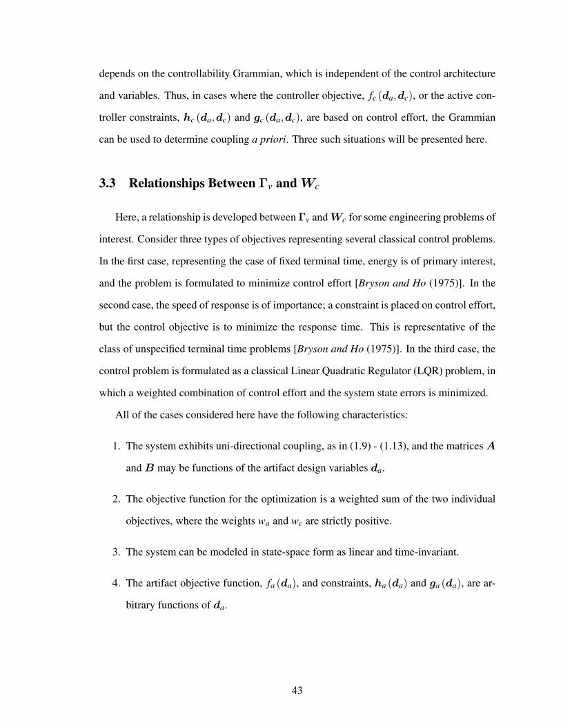
depends on the controllability Grammian, which is independent of the control architecture
and variables. Thus, in cases where the controller objective, fc (da,dc), or the active con-
troller constraints, hc (da,dc) and gc (da,dc), are based on control effort, the Grammian
can be used to determine coupling a priori. Three such situations will be presented here.
3.3 Relationships Between Γv andWc
Here, a relationship is developed between Γv andWc for some engineering problems of
interest. Consider three types of objectives representing several classical control problems.
In the first case, representing the case of fixed terminal time, energy is of primary interest,
and the problem is formulated to minimize control effort [Bryson and Ho (1975)]. In the
second case, the speed of response is of importance; a constraint is placed on control effort,
but the control objective is to minimize the response time. This is representative of the
class of unspecified terminal time problems [Bryson and Ho (1975)]. In the third case, the
control problem is formulated as a classical Linear Quadratic Regulator (LQR) problem, in
which a weighted combination of control effort and the system state errors is minimized.
All of the cases considered here have the following characteristics:
1. The system exhibits uni-directional coupling, as in (1.9) - (1.13), and the matricesA
andB may be functions of the artifact design variables da.
2. The objective function for the optimization is a weighted sum of the two individual
objectives, where the weights wa and wc are strictly positive.
3. The system can be modeled in state-space form as linear and time-invariant.
4. The artifact objective function, fa (da), and constraints, ha (da) and ga (da), are ar-
bitrary functions of da.
43

3.3.1 Case I: Control Effort as Objective
In Case I, the primary concern in controller design is energy. The system is to be moved
from the origin to a state x f at time t f , where t f is a parameter. In the most general case,
the final state x f may be a function of da. The control objective function to accomplish
this is selected as the control effort required to move the system from the origin to a state
x f at some specified time t f .
fc =
t f∫0
u(t)2dt (3.9)
Using (3.6) and (3.9), the controller objective function fc will satisfy the relation
fc ≥ xTfWc
(t f)−1
x f (3.10)
where the equality applies if an optimal controller that minimizes control effort is chosen.
The coupling vector is computed from (1.14) as follows:
Γv =wc
wa
∂
∂da
(xT
fWc(t f)−1
x f
)(3.11)
Γv =wc
wa
xTf
∂Wc(t f)−1
∂da1
x f +2xTfWc
(t f)−1 ∂x f
∂da1
xTf
∂Wc(t f)−1
∂da2
x f +2xTfWc
(t f)−1 ∂x f
∂da2...
xTf
∂Wc(t f)−1
∂dan
x f +2xTfWc
(t f)−1 ∂x f
∂dan
T
(3.12)
where da is indexed as i = 1, . . . ,n and n is the number of artifact design variables. Given
a particular system, then, it is possible to express the coupling in terms of the artifact
design variables da, constants, and parameters in the problem. Given the known values
of constants and parameters, and the range of allowable values for da, it is possible to
44

determine whether coupling will exist, and whether it will be weak or strong. If the ith
term in the coupling vector vanishes, then it is known that the ith artifact design variable
will not participate in the coupling. If all terms in the coupling vector vanish, then the
problem is known to be uncoupled. A particular coupling term will vanish under one of
two conditions:
1. The vectors x f and
(2Wc
(t f)−1 ∂x f
∂dai
+∂Wc
(t f)−1
∂dai
x f
)are orthogonal.
2.∂x f
∂dai
=−12Wc(t f) ∂Wc
(t f)−1
∂dai
x f .
The second condition can occur when the variables da result in changes in the control
effort that counteract the effects of the changes in x f . As an example, a change in da
might simultaneously cause an increase in x f and an increase in mechanical advantage.
The improvement in mechanical advantage would balance the increase in the final state,
resulting in constant control effort for the optimal controller.
Within the class of problems denoted here as Case I, there are two sub-classes that are
of interest.
Case Ia: Final State as a Parameter: If the final state x f is a specified parameter, then
the expression given in (3.12) can be simplified to
Γv =wc
wa
xTf
∂Wc(t f)−1
∂da1
x f
xTf
∂Wc(t f)−1
∂da2
x f
...
xTf
∂Wc(t f)−1
∂dan
x f
T
(3.13)
If Wc is not a function of da, then∂Wc
(t f)−1
∂da= 0 for any value of da. In this case,
each of the components in this relation will vanish. Therefore, Γv = 0, and the system
is uncoupled. Note, however, that while this is a sufficient condition for decoupling, it is
45

not necessary and sufficient. It is still possible for the system to decouple if∂W−1
c∂da
6= 0.
Specific values of x f may cause particular terms to drop out of the final result, or the vector∂W−1
c∂da
x f may be orthogonal to x f .
Case Ib: Constant Controllability Grammian: Assume that the controllability Gram-
mian Wc is not dependent on da. This may occur when the variables da represent conver-
sions from one form of energy to another, which will not change the total effort required to
control the system. Then, the coupling vector Γv can be expressed as
Γv =wc
wa
2xTfWc
(t f)−1 ∂x f
∂da1
2xTfWc
(t f)−1 ∂x f
∂da2...
2xTfWc
(t f)−1 ∂x f
∂dan
T
(3.14)
In this case, a term in the coupling vector will vanish in either of two conditions. The
first condition,∂x f
∂dai
= 0, represents the case where neither x f nor Wc(t f)
is a function
of da, and thus E∗ is independent of da. In the second condition, the vectors∂x f
∂dai
and
Wc(t f)−1
x f are orthogonal.
Positioning Gantry Example: For the positioning gantry described in Chapter II, the
following objectives and constraints are selected:
minkt ,r
fa =−Z f (kt ,r) (3.15)
subject to simple bounds 2.5≤ r ≤ 7.5 (3.16)
5≤ kt ≤ 20 (3.17)
where the final displacement Z f represents the peak displacement, with a 10% overshoot
over the steady-state displacement, Zss. The equation for the steady-state displacement, Zss,
46

is derived in Chapter II. Thus,
Z f = 1.1Zss =1.1usskt
rRaks(3.18)
The final state, x f , is therefore given by
x f =
Z f
0
. (3.19)
It is desired to minimize the control effort required to move the system to this position at a
specified time, t f = 0.5s, and thus the controller objective is
minK1,K2,G
fc =
t f∫0
(u(t))2 dt. (3.20)
This optimization problem fits the description for a Case I problem. The controllability
GrammianWc(t f)
of this system is given by
Wc(t f)
=
Wc11
(t f)
Wc12
(t f)
Wc21
(t f)
Wc22
(t f) (3.21)
where the individual terms are as follows:
Wc11
(t f)
=1
2bk− 2me−
bm t f
b(4mk−b2)+
e−bm t f
2k√
4mk−b2sin(√
4mk−b2 t f
m
)+
e−bm t f
2k (4mk−b2)cos(√
4mk−b2 t f
m
) (3.22)
Wc12
(t f)
=e−
bm t f
4mk−b2
(1− cos
(√4mk−b2 t f
m
))(3.23)
47

Wc21
(t f)
=e−
bm t f
4mk−b2
(1− cos
(√4mk−b2 t f
m
))(3.24)
Wc22
(t f)
=1
2bm− 4ke−
bm t f
b(4mk−b2)+
e−bm t f
m(4mk−b2)3/2 sin(
t f
m
√4mk−b2
)
− be−bm t f
m(4mk−b2)cos(
t f
m
√4mk−b2
) (3.25)
Expressions for m, b, and k are given by Eqs. (2.19) - (2.21). Using these expressions, it
can be shown that Wc(t f)
is a function of r and kt , as is x f . Taking derivatives of both
x f and Wc(t f)
with respect to da, it can be shown that there are no feasible values of
r and kt for which Γv = 0. Therefore, it is concluded that the problem will be coupled,
and an appropriate solution method for a coupled problem should be chosen. When the
simultaneous co-design problem is solved, it is indeed seen to be coupled, with the expected
tradeoff between the objectives shown in Fig. 3.1.
3.3.2 Case II: Time as Objective
In Case II problems, the primary concern is the speed with which the system responds;
or, alternatively, the final time at which the system reaches the state x f is to be minimized.
Control effort is constrained to be less than some maximum value, Emax, where Emax is a
parameter. The controller objective function and constraint are as follows:
minda,dc
fc = t f (3.26)
subject to gc (da,dc) =
t f∫0
u(t)2dt−Emax ≤ 0 (3.27)
It can be assumed that the constraint will be active, since a linear system could have an
arbitrarily small response time if infinite control effort were available. Assuming that the
48

Figure 3.1: Pareto Frontier for Positioning Gantry Example of Case I
constraint is active and that an optimal controller is chosen,
xTfWc
(t f)−1
x f = Emax. (3.28)
Taking derivatives of (3.28) and solving for∂ t f
∂dai
,
∂ t f
∂dai
=−2xT
fWc(t f)−1 ∂x f
∂dai
+xTf
∂Wc(t f)−1
∂dai
x f
2xTfWc
(t f)−1 ∂x f
∂ t f+xT
f∂Wc
(t f)−1
∂ t fx f
(3.29)
49

the coupling can be expressed as
Γv =− wc
waT
2xTfWc
(t f)−1 ∂x f
∂da1
+xTf
∂Wc(t f)−1
∂da1
x f
2xTfWc
(t f)−1 ∂x f
∂da2
+xTf
∂Wc(t f)−1
∂da2
x f
...
2xTfWc
(t f)−1 ∂x f
∂dan
+xTf
∂Wc(t f)−1
∂dan
x f
T
(3.30)
where T = 2xTfWc
(t f)−1 ∂x f
∂ t f+xT
f∂Wc
(t f)−1
∂ t fx f .
Note that the coupling vector is parallel to that seen for Case I, and the conditions for
decoupling in this problem are mathematically identical. This indicates that the physical
conditions under which the problems decouple are also the same. As in Case I, therefore,
one situation which would result in decoupling is that in which changes in da produce both
a greater displacement x f of the system and a more efficient use of the available control
effort. Within this class of problems, there are two sub-classes of interest, similar to those
discussed for Case I.
Case IIa: Final State as a Parameter: If the final state x f is a parameter, then the
coupling simplifies to
Γv =− wc
wa
(xT
f∂Wc
(t f)−1
∂ t fx f
)
xTf
∂Wc(t f)−1
∂da1
x f
xTf
∂Wc(t f)−1
∂da2
x f
...
xTf
∂Wc(t f)−1
∂dan
x f
T
(3.31)
and the coupling vector is parallel to that seen in Case Ia, with identical conditions for
decoupling.
Constant Controllability Grammian: Assume that the controllability Grammian matrix
50

Wc(t f)
is not dependent on da. As in Case I, this can happen when da represents the
conversion of energy with no loss. Then, the coupling vector Γv can be expressed as
Γv =− wc
wa
(xT
fWc(t f)−1 ∂x f
∂ t f
)
xTfWc
(t f)−1 ∂x f
∂da1
xTfWc
(t f)−1 ∂x f
∂da2...
xTfWc
(t f)−1 ∂x f
∂dan
T
(3.32)
and, in this case, the coupling vector is parallel to that seen in Case Ib, with identical
conditions for decoupling.
Positioning Gantry Example: Assume, in this case, that the artifact design objective
and constraints are as given in Eqs. (3.15) - (3.17). The controller design objective and
constraints are as follows:
minK1,K2,G
fc = t f (3.33)
subject to
g1 (K1,K2,G) =
t f∫0
(u(t))2 dt−Emax ≤ 0 (3.34)
Monotonicity analysis indicates that the constraint g1 will be active, and therefore this prob-
lem meets the conditions established for Case II. The controllability Grammian is given by
Eqs. (3.21)-(3.25). In this case, the coupling is again non-zero for every allowed value of r
and kt . When the problem is solved, the anticipated tradeoff between fa and fc is evident,
as shown in Fig. 3.2.
3.3.3 Case III: Linear Quadratic Regulator (LQR)
The infinite-time LQR problem is designed to find the optimal control signal u(t) to
transition a system from an initial state x0 = x(0) to the zero state. The optimal control
51
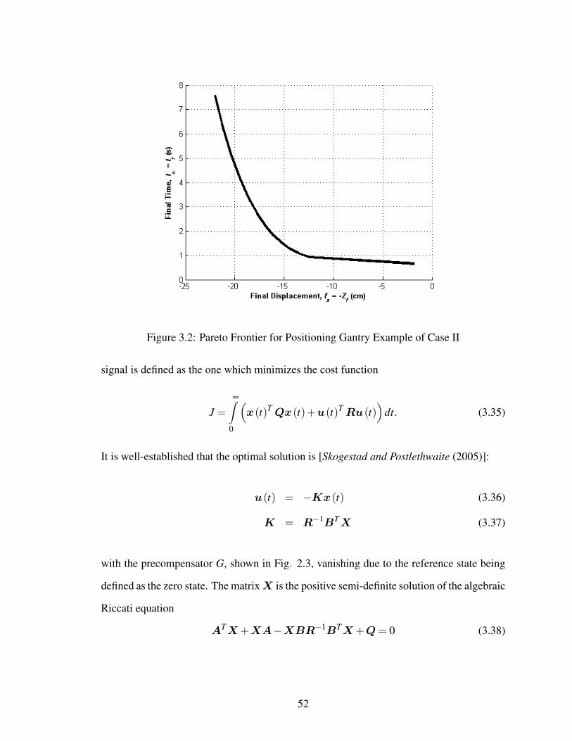
Figure 3.2: Pareto Frontier for Positioning Gantry Example of Case II
signal is defined as the one which minimizes the cost function
J =∞∫
0
(x(t)T Qx(t)+u(t)T Ru(t)
)dt. (3.35)
It is well-established that the optimal solution is [Skogestad and Postlethwaite (2005)]:
u(t) = −Kx(t) (3.36)
K = R−1BTX (3.37)
with the precompensator G, shown in Fig. 2.3, vanishing due to the reference state being
defined as the zero state. The matrixX is the positive semi-definite solution of the algebraic
Riccati equation
ATX+XA−XBR−1BTX+Q= 0 (3.38)
52

and the optimal value of J is given by the equation
J∗ = xT0Xx0. (3.39)
If the system is controllable, then it has also been proven that there exists a reduced equiv-
alent transformation of the system, and the symmetric matrix X satisfies the Lyapunov
equation [Ionescu et al. (1999)]:
ATX+XA+Q= 0 (3.40)
In the most general case, whereQ can be selected as any positive semidefinite matrix, there
is no explicit relation between J∗ and W∞c , and thus no explicit relation between Γv and
W∞c . However, if the matrixQ is selected as
Q= γBBT , (3.41)
as is common in loop-transfer recovery design [Skogestad and Postlethwaite (2005)], then
by comparing Eq. (3.5) and (3.40), it can be shown that the matrix X can be expressed in
terms of the controllability Grammian as [Skogestad and Postlethwaite (2005)]:
X = γA−TAW∞c (3.42)
and, therefore, the optimal performance is
J∗ = γxT0A−TAW∞
c x0. (3.43)
53

This allows the coupling to be derived as
Γv = γwc
wa
∂(xT
0A−TAW∞
c x0)
∂da1∂(xT
0A−TAW∞
c x0)
∂da2...
∂(xT
0A−TAW∞
c x0)
∂dan
T
(3.44)
This expression for Γv is, again, a function only of the artifact design variables. It is
important to note that this expression is only valid for the specific form of Q given by Eq.
(3.41). For other forms of Q, Eq. (3.42) is not valid. It is conjectured that more complex
relations between X and W∞c may be found for some other forms of Q, and thus other
relationships between coupling and controllability may hold for other cases of the LQR
problem.
While Eq. (3.44) is a complex expression, in general, depending on the problem in
question, it can simplify under certain circumstances. One particular situation is detailed
below, in which it takes on a considerably simpler form.
Case IIIa: State x0 as a parameter and A independent of da: If the forced response
of a system is a function of da but the free response is not, then the B matrix will be a
function of da but A will be independent of da. If, in addition, the state x0 is a parameter,
the coupling relation is given by
Γv = γwc
wa
xT0A−TA
∂W∞c
∂da1
x0
xT0A−TA
∂W∞c
∂da2
x0
...
xT0A−TA
∂W∞c
∂dan
x0
T
(3.45)
Note that, in this case, there are several conditions in which decoupling will occur.
54

1. For all artifact design variables da, the derivative∂W∞
c∂dai
= 0.
2. The matrix productA−TA∂W∞
c∂dai
= 0 for all artifact design variables da.
3. The vectors x0 and(A−TA
∂W∞c
∂dai
x0
)are orthogonal for all artifact design vari-
ables da.
Positioning Gantry Example: Consider, again, the positioning gantry system shown in
Chapter II. In this case, the artifact objective function is assumed to be the system’s total
weight. The weight depends on a number of system parameters, which shall be grouped
into three constants for simplicity. The artifact objective then takes the form of
minr,kt
fa = c1 + c2k1.5t + c3r2 (3.46)
where c1 = 10, c2 = 5, and c3 = 0.1, subject to the bounds given in Eqs. (3.16) - (3.17).
Note that the pulley was assumed, in Section 2.3, to possess negligible rotational inertia;
however, it is not assumed to be massless, and thus it appears in the calculation of system
weight. The controller optimization problem is formulated as an LQR problem with con-
troller objective fc = J, where J is given by Eq. (3.35) with x0 =
3.5
0
, R = 1, and
Q=
0 0
0 1
. It can be shown that this choice of weighting matrixQ satisfies Eq. (3.41),
with γ = m2. Using Eq. (3.44), the coupling can be computed for this problem. In this case,
the coupling can be shown to vanish for all values of r and kt , indicating that the problem
is uncoupled and that J∗ is independent of these variables. Note that this is not a result
that could be easily seen, though it can be explained physically; the variable r, the pulley
diameter, represents a conversion of energy without loss, and the variable kt , the motor
torque constant, represents a tradeoff between the motor’s speed and torque, which entails
no loss of energy. When the co-design problem is solved for the values of parameters given
55

Table 3.1: Parameters for Optimization of Gantry Using LQR Control
Parameter ValueRa 2.0 kΩ
M 2.0 kgks 2.0 N/mmVss 10 V
Table 3.2: Results of Optimization of Gantry Using LQR Control
Quantity Valuer 2.5 cmkt 5.0 N-m/AK1 -0.368K2 -7.696G 0.132f ∗a 66.53f ∗c 5.78
in Table 3.1, no tradeoff is seen. For all values of wa and wc, the variables and objectives
are found to have the values shown in Table 3.2.
3.4 Physical Demonstration: Positioning Gantry
The positioning gantry system described in Chapter II, and used to illustrate the con-
cepts in this chapter and in Chapter II, was built and used for an experimental demon-
stration. The demonstration was designed to show that it is possible to predict, a priori,
whether a problem will be coupled. In this section, the apparatus used for the demonstra-
tion will be described. The intention of the demonstration will be described, and results
will be shown.
3.4.1 Description of Apparatus
The apparatus for the physical demonstration was constructed using a Quanser En-
gineering Trainer DC Motor Control Trainer (QET-DCMCT), as shown in Fig. 3.3. The
56
QET-DCMCT unit consists of a motor, encoder, associated electrical components, and soft-
ware (item 1). A plate, item 2, was mounted to the QET-DCMCT unit. A linear rail, item
3 was mounted to the plate, and an angle bracket, item 4, was mounted to the block that
mates with the rail. A spring, item 5, was attached at one end to item 4 and at the other end
to a fixed bracket, item 6. A synchronous belt, item 8, was clamped to item 6 and driven
by a pulley, item 7, which was mounted to the QET-DCMCT motor.
Figure 3.3: Apparatus for Physical Demonstration of Gantry Example (Item 1: QET motorassembly, Item 2: mounting plate, Item 3: linear rail, Item 4: angle bracket,Item 5: extension spring, Item 6: fixed mounting bracket, Item 7: pulley)
The spring corresponds to the spring with constant ks shown in Fig. 2.2. The bracket
and linear block correspond to the mass, M. The timing pulley corresponds to the pulley of
radius r, and the QET-DCMCT unit corresponds to the motor with armature resistance Ra
and torque constant kt . It was assumed that the inertia of the pulley is negligible, and that
57

the friction between the block and rail is negligible.
The system was run by means of the supplied QET-DCMCT software. This software
allows the user to specify the gains integral gain ki, derivative gain kd , and proportional
gain kp, as shown in Fig. 3.4. This controller is different from the controller shown in Fig.
2.3. The QET-DCMCT controller has integral control instead of a precompensator. The
gain kp is equivalent to the gain K1, and kd is equivalent to K2. However, the controllability
Grammian is still capable of predicting whether or not the system will be coupled, since it
is independent of the control architecture.
3.4.2 Demonstration Procedure
This system corresponds to the positioning gantry shown in Fig. 2.2. As discussed in
Sections 2.3.2 and 3.3, the co-design of this system will be a coupled problem for certain
choices of artifact design variables. In particular, the spring constant, ks, shall be studied for
this demonstration. An optimization problem of the type described as Case I is formulated.
It can be shown from Eq. (3.12) that this problem will be coupled. The results of this
demonstration confirm this result.
The spring strength was varied by operating the system once with a single spring with
ks = 0.81 lbs/in, and a second time with two springs in series, as shown in Fig. 3.5. This
has the effect of decreasing the spring constant by a factor of 2, to ks = 0.40 lbs/in. The
position command to the controller was a step input with a fixed terminal time for the
system. The terminal time, t f , was held constant at t f = 2.5 sec.
The control objective function fc, was the control effort, which was to be minimized.
The final position of the system, Z f , was a parameter with the value of Z f = 0.3 in. The
control objective, then, can be expressed as
minkp,kd ,ki
fc = E =
t f∫0
(V (t))2 dt (3.47)
58

Figure 3.4: Control Screen for QET-DCMCT Software
59
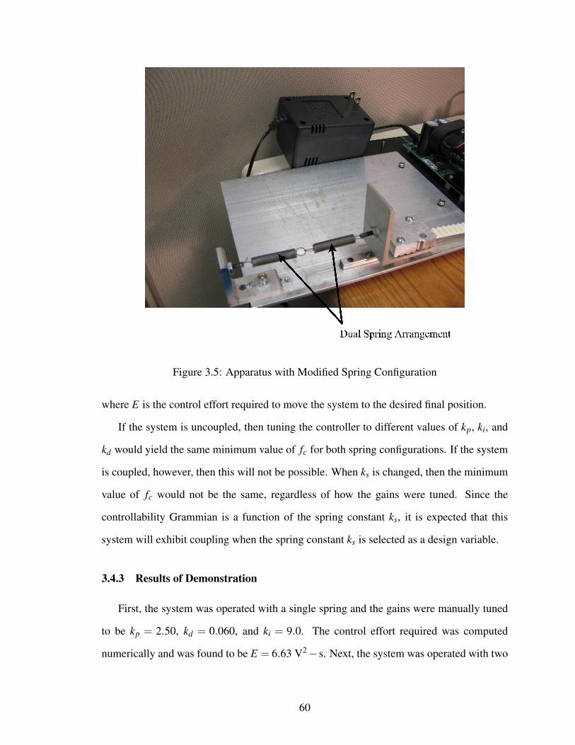
Figure 3.5: Apparatus with Modified Spring Configuration
where E is the control effort required to move the system to the desired final position.
If the system is uncoupled, then tuning the controller to different values of kp, ki, and
kd would yield the same minimum value of fc for both spring configurations. If the system
is coupled, however, then this will not be possible. When ks is changed, then the minimum
value of fc would not be the same, regardless of how the gains were tuned. Since the
controllability Grammian is a function of the spring constant ks, it is expected that this
system will exhibit coupling when the spring constant ks is selected as a design variable.
3.4.3 Results of Demonstration
First, the system was operated with a single spring and the gains were manually tuned
to be kp = 2.50, kd = 0.060, and ki = 9.0. The control effort required was computed
numerically and was found to be E = 6.63 V2− s. Next, the system was operated with two
60

Figure 3.6: Voltage for Single and Dual Spring Configurations
springs, and the gains were tuned to minimize the control effort. The resulting gains were
found to be kp = 1.20, kd = 0.030, and ki = 6.5. The control effort required was computed
numerically and was found to be E = 5.74 V2−s. The voltage and position graphs for both
configurations are given in Fig. 3.6 and 3.7, respectively.
Since the gains were tuned manually, no guarantee of optimality can be given. How-
ever, it can be seen from Fig. 3.7 that the position responses are very similar for both spring
configurations, and thus the voltage required for each case can be compared on an equal
basis. The control effort is the area under the curve; from Fig. 3.6, it can be seen that this
area will be larger for the single spring configuration than for the dual spring configuration.
Therefore, the control objective function, fc, is a function of the spring constant, ks. Thus,
coupling is present, as predicted based on Eq. (3.12). It can thus be seen that the relation-
ships presented between coupling and controllability are an effective tool in the analysis of
a co-design problem prior to optimization.
61

Figure 3.7: Position Response for Single and Dual Spring Configurations
3.5 Summary
As shown in this chapter, it is often possible to determine a priori whether or not a
co-design problem exhibits coupling. If the control objective, fc (da,dc), or the active con-
troller constraints, hc (da,dc) or gc (da,dc), depend on control effort, then that objective or
constraint can be related to the controllability Grammian matrix. This allows the coupling
to be determined, without solving the co-design problem or even specifying the controller
architecture, due to the relationship between the controllability Grammian and the optimal
control performance. Three specific classical optimal control problem formulations were
presented here; it is anticipated that other problem formulations can be found in which cou-
pling can be similarly related to controllability. The experiment conducted on the gantry
example showed that these relationships can be used to predict whether or not a co-design
problem will be coupled.
If the problem is uncoupled, then a sequential strategy can be used and will find the
62

system optimal solution. If the problem is coupled, then an appropriate solution strategy
can be chosen. A variety of solution strategies for coupled problems have been proposed,
as discussed in Chapter I. A new strategy for co-design problems with uni-directional
coupling will be proposed in the following chapter, utilizing the concept of a Control Proxy
Function. The relations between coupling and controllability developed in this chapter will
also be useful in the development of the Control Proxy Functions that will be proposed for
solving the co-design problem.
63

CHAPTER IV
Design for Ease of Control Using Control Proxy Functions
4.1 Introduction
In Chapter III, the issue of identifying coupling a priori in co-design problems was
addressed. If coupling is not present, then a sequential solution strategy will produce a
system-optimal solution. However, if coupling is present, this is not the case. A simultane-
ous formulation, if it can be solved, will produce system-optimal results, but this approach
has some significant disadvantages due to computational and organizational complexity.
An ideal approach would produce the same results as those found with the simultaneous
formulation, but would exhibit the simplicity of the sequential formulation. Therefore, in
this chapter a modified sequential solution strategy is proposed, in which the original arti-
fact objective function, fa, is augmented by a Control Proxy Function (CPF), representing
the system’s ease of control. The CPF, denoted as χ , is a function only of the artifact de-
sign variables da and not of the control design variables dc. The bi-objective artifact design
problem with the two functions fa (da) and χ (da) may be solved in a variety of ways, as
discussed in the multi-objective optimization literature [e.g., Das and Dennis (1997), Mes-
sac and Puemi-Sukam (2000), Kitayama et al. (2009), Steuer (1986)]. In this chapter, a
weighted linear combination will be used to demonstrate the proposed method.
The modified sequential problem formulation, termed the CPF problem, is expressed
64

as
minda
f ′a (da) = w1 fa (da)+w2χ (da) (4.1)
subject to ga (da)≤ 0 (4.2)
ha (da) = 0 (4.3)
followed by the control design problem
mindc
fc (d∗a,dc) (4.4)
subject to gc (d∗a,dc)≤ 0 (4.5)
hc (d∗a,dc) = 0 (4.6)
where d∗a = argmin f ′a (da). The problem formulation can also be represented graphically,
as in Fig. (4.1)
Figure 4.1: Control Proxy Function Problem Formulation
Of course, the goal in solving the modified sequential problem illustrated in Fig. 4.1
65

is to select the CPF, χ (da), in such a way that the solution to this problem is ‘close’ to
the system optimal solution that would be obtained by solving the original simultaneous
problem in Eq. (1.9) - (1.13).
4.2 Characteristics of Effective Control Proxy Functions (CPFs)
The choice of an appropriate control proxy function (CPF), χ (da), is critical in formu-
lating the modified sequential optimization problem. A well-chosen CPF, which effectively
captures the fundamental physical limitations of the system, will result in solutions that are
close to the Pareto optimal points found by a simultaneous formulation, while a poorly
chosen CPF will yield solutions that are far from system optimality. Clearly, the selected
CPF must not require knowledge of the controller design.
This raises the questions of how to determine the ’closeness’ of a CPF solution to
the Pareto frontier, and how to formulate an appropriate CPF. The closeness of the CPF
solution should be determined without solving the simultaneous formulation for Pareto
optimal points, since the motivation for the CPF formulation is to eliminate the need to
solve the simultaneous problem. A suitable measure of the CPF solution’s closeness can
be found by evaluating the angle ξ between two vectors that can be calculated at any point
of the CPF solution set. The two vectors which define ξ are ∇χ =∂ χ
∂da, the gradient
of the CPF, and Γv, the estimate of the coupling vector. The equation for calculating Γv
is identical to that for Γv; however, since the coupling vector is valid only at an optimal
solution to the system, the vector found at a CPF point is an estimate. It is then shown
that this measure of closeness to optimality can be used to justify two conditions that an
effective CPF will satisfy. The issues of evaluating a CPF and of selecting an appropriate
CPF are summarized in the four items listed below.
1. If Γv is parallel to ∇χ at all points, then the CPF solution set will coincide with the
Pareto frontier.
66

2. CPF solution points will approach the Pareto frontier as ξ , the angle between the
estimate of the coupling vector Γv and ∇χ in the da-space, approaches zero; i.e.,
CPF solution points will be close to the Pareto frontier when the angle ξ is small.
3. If the control objective function, fc (da,dc), is monotonic with respect to some ele-
ment of da, then an effective CPF, χ (da), will have the same coordinate-wise mono-
tonicity as fc with respect to that element of da.
4. If the control objective function, fc (da,dc), has an unconstrained minimum in the
da-space, then an effective CPF, χ (da), will obtain its minimum close to it.
Each of these four items will be discussed in more detail in the following subsections,
with mathematical examples given to illustrate the concepts. The items are stated as theo-
rems; proof of each theorem is given in Appendix A.
4.2.1 Characterization of a Perfect CPF
A CPF will be described as ‘perfect’ if every solution of the CPF problem is also a
solution to the simultaneous problem given in Eq. (1.9) - (1.13), i.e., every CPF point will
coincide with the Pareto frontier. The condition which ensures that this will occur is stated
as a theorem, followed by an example. The proof of the theorem is given in Appendix A.
THEOREM 4.1: If Γv ‖∇χ for all solutions to the CPF problem given in Eq. (4.1) - (4.3),
then all solutions to the CPF problem will also be solutions to the simultaneous problem
given in Eq. (1.9) - (1.13).
EXAMPLE: To illustrate the relationship between Γv and ∇χ , consider the following
67

coupled optimization problem:
minwa fa (da)+wc fc (da,dc) (4.7)
fa (da) = 0.5d2a1
+d2a2−da1da2−7da1−7da2 (4.8)
fc (da,dc) = (da1−da2)2 +
19
(da1 +da2 +dc−10)2 +(dc−5)2 (4.9)
subject to ga (da) = 4d2a1
+d2a2−900≤ 0 (4.10)
A CPF of
χ (da) = 11d2a1
+11d2a2−18da1da2−10da1−10da2 +25 (4.11)
is chosen, and the system is optimized both sequentially and simultaneously.
The coupling vector Γv is given by the relation
Γv =2wc
9wa
10da1−8da2 +dc−10
−8da1 +10da2 +dc−10
T
da = d∗a
dc = d∗c
(4.12)
and the CPF has the gradient
∇χ =
22da1−18da2−10
−18da1 +22da2−10
T
(4.13)
Since there are no controller constraints gc (da,dc) or hc (da,dc),∂ fc
∂dc= 0, and therefore
dc = 5.5−0.1da1−0.1da2 . (4.14)
68

Substituting into Eq.(4.12),
Γv =2wc
wa
1.1da1−0.9da2−0.5
−0.9da1 +1.1da2−0.5
T
da = d∗a
dc = d∗c
(4.15)
It can be readily seen that, at any da that solves the simultaneous problem,
Γv = 10wc
wa∇χ (4.16)
and therefore it is anticipated that the use of this CPF will duplicate the Pareto frontier.
This is indeed the case, as shown by the numerical results in Fig. 4.2.
Figure 4.2: Comparison of Simultaneous and CPF Solutions for Γv ‖ ∇χ
69

4.2.2 Quantification of the ‘Closeness’ of a CPF Point to the Pareto Frontier
As stated above, a perfect CPF is characterized by ∇χ ‖ Γv, i.e., when the angle ξ
between ∇χ and Γv is zero. This suggests that ξ may serve as a means of evaluating
the fidelity of a given CPF in modeling the behavior of fc. If a CPF is not perfect, but it
provides near-optimal results, then it can be useful when achieving true optimality would
take significant additional computational effort. The condition which allows the use of ξ
to characterize the closeness of a CPF is stated as a theorem, with the proof given in Ap-
pendix A. Note that the proof is valid only if no artifact constraints ga (da), ha (da) are
active. However, it can be shown that the relation is true for some problems with active
constraints on the artifact. Since constraints act to reduce the degrees of freedom present in
an optimization problem, it is conjectured that, in the presence of constraints, the angle ξ
will represent an upper bound on the ‘distance’ between a CPF point and the Pareto fron-
tier. An example is given following the statement of the theorem.
THEOREM 4.2: If a co-design problem, as given in Eq. (1.9) - (1.13), is convex and no
artifact constraints ga (da), ha (da) are active, then the angle ξ between ∇χ and the esti-
mated coupling vector Γv at a CPF point will be monotonically related to ε , the distance
between that CPF point and the nearest Pareto optimal point, measured in the da-space.
EXAMPLE: Consider the following problem:
minwa fa (da)+wc fc (da,dc) (4.17)
fa (da) = 0.5d2a1
+d2a2−da1da2−7da1−7da2 (4.18)
fc (da,dc) = (da1−da2)2 +
19
(da1 +da2 +dc−10)2 +(dc−5)2 (4.19)
A CPF of
χ1 (da) = (da1−5)2 +d2a2−25 (4.20)
70

is chosen, and the system is optimized both sequentially and simultaneously. The angle ξ
is compared with the distance ε to the nearest point on the true Pareto frontier in Fig. (4.3),
and it can be seen that, for this example, this angle is an effective measure of the distance to
the frontier. Using this measure, the accuracy of a CPF can be evaluated without knowing
the true Pareto frontier.
Figure 4.3: Comparison of angle ξ and distance ε
4.2.3 Monotonicity of Controller Objective and CPF
A function is said to be coordinate-wise monotonic if it is either always increasing
or always decreasing with respect to a given variable, e.g., if the partial derivative of a
continuous function does not change sign [Papalambros and Wilde (2000)]. Monotonicity
analysis is a useful tool in optimization problems. For example, it can be used to determine
constraint activity, to study the behavior of composite functions, and to give insight into
the tradeoffs present in optimization problems [Papalambros and Wilde (2000)]. Here, we
use monotonicity to characterize effective CPFs.
If a controller objective fc (da,dc) is monotonic with respect to an element of da, then
71

it seems logical that χ (da) should have the same monotonicity with respect to that element
of da in order to effectively model the behavior of fc. This is the case, as stated in Theorem
4.3 below. An example follows the theorem, and the proof is given in Appendix A.
THEOREM 4.3: If fc (da,dc) is monotonic with respect to some element of da, and that
element of da does not appear in any active constraint, then a CPF with the same mono-
tonicity will produce closer solutions than a CPF with the opposite monotonicity.
EXAMPLE: Consider the following problem:
minwa fa (da)+wc fc (da,dc) (4.21)
fa (da) = 0.5d2a1
+d2a2−da1da2−7da1−7da2 (4.22)
fc (da,dc) = da1 +da2−dc (4.23)
subject to
ga (da) = 10−da1−da2 ≤ 0 (4.24)
gc (da,dc) =(
da2−dc
2
)2
−25≤ 0 (4.25)
where da = da : da ≥ 0.
A CPF of
χ (da) = da1 +0.25d0.5a2
(4.26)
is chosen. It is evident that fc and χ are both monotonically increasing with respect to da1
and da2 . Solving both the simultaneous optimization and the CPF problem, it can be seen in
Fig. 4.4 that the CPF solution models the tradeoff between fa and fc, though imperfectly.
In contrast, consider a CPF of
χ (da) =−da1 +0.25d0.5a2
(4.27)
72

Figure 4.4: Comparison of Simultaneous and CPF Solutions for Appropriate Monotonicity
In this case, the monotonicity of χ and fc with respect to da1 does not match. Solving the
new CPF problem, it can be seen in Fig. 4.5 that this CPF does not model the tradeoff
between fa and fc.
4.2.4 Locations of Unconstrained Minima of fc and χ
In the previous section, fc was assumed to be monotonic with respect to some element
of da. Here, we consider the case where fc is not monotonic, but rather has an uncon-
strained minimum. Intuitively, it seems likely that the values taken by da at the minimum
of fc should also minimize χ , and that a CPF will become less effective if the minimum
of χ is farther from the minimum of fc in the da-space. This can be proven for an uncon-
strained problem, and it is conjectured that it will also be true for constrained problems.
This condition is stated as a theorem, with the proof given in Appendix A. The theorem is
followed by an example.
73

Figure 4.5: Comparison of Simultaneous and CPF Solutions for Inappropriate Monotonic-ity
THEOREM 4.4: Assume that fc (da,dc) has an unconstrained minimum, and that χ (da)
is chosen such that it has an unconstrained minimum. Then, the distance between a CPF
point and the Pareto frontier will increase as the distance increases between the minima of
fc and χ .
EXAMPLE: Consider the following problem:
minwa fa (da)+wc fc (da,dc) (4.28)
fa (da) = 0.5d2a1
+d2a2−da1da2−7da1−7da2 (4.29)
fc (da,dc) = (da1−da2)2 +
19
(da1 +da2 +dc−10)2 +(dc−5)2 (4.30)
subject to
ga (da) = 4d2a1
+d2a2−900≤ 0 (4.31)
gc (da,dc) =1
50d2
a1+
15
d2a2−48≤ 0 (4.32)
74

Table 4.1: Comparison of Minima of Objective Functions and Control Proxy Functions
da1 da2
fa 21 14fc 2.5 2.5χ1 5 0χ2 1 -10
This problem is solved twice, with two different CPFs, which will then be compared.
χ1 (da) = (da1−5)2 +d2a2−25 (4.33)
χ2 (da) = (da1−1)2 +(da2 +10)2−10 (4.34)
The unconstrained minima of the functions fa, fc, χ1, and χ2 are given in Table 4.1.
The solutions found by solving the two CPF sequential problems are shown in Fig. 4.6. It
can be seen that χ1, which obtains its minimum closer to that of fc than does χ2, produces
a closer match to the simultaneous solution than χ2.
Figure 4.6: Comparison of Simultaneous and CPF Solutions for Two Choices of CPF
75

4.3 Control Proxy Functions for Specific Co-Design Problem Formu-
lations
Given the characteristics of effective CPFs that have been developed in Section 4.2, we
can formulate potential CPFs for specific problem formulations and evaluate them. In this
section, we will show that a perfect CPF exists for each of several problem formulations.
Of course, the formulations considered here are not exhaustive. There are many co-design
problem formulations that are not considered here, and it is anticipated that future work
will identify additional CPFs that would be useful for additional problem formulations.
The CPFs evaluated here will be based on either the natural frequency of the system or
on the controllability Grammian matrix. The natural frequency is considered as the basis for
a CPF because previous work has shown that, in some cases, it can be used as an effective
proxy for a system’s ease of control [e.g., Peters et al. (2008), Hale et al. (1985), Khot and
Abhyankar (1993), Bodden and Junkins (1985), Yee and Tsuei (1991)]. The controllability
Grammian matrix, Wc, will be considered as the basis for a CPF because previous work,
as described in Chapter III and in [Peters et al. (2010)], has shown that, for some problem
formulations, there is a relationship betweenWc and the coupling vector Γv. Since there is
also a relationship between Γv and an effective CPF, this suggests that a CPF based onWc
will be effective for some problems.
4.3.1 Natural Frequency as a Control Proxy Function
Since the natural frequency of a system depends only on the artifact and can be used, in
some cases, to model the system’s ease of control, there will be problems for which an ef-
fective control proxy function χ (da) will be a function of the natural frequency. This raises
the question of when a CPF of this type would be effective. There are several necessary
conditions for a CPF based on natural frequency to be effective. Those that are common to
all of the cases discussed in this section are listed below.
76

1. The co-design problem is formulated as in Eq. (1.9)-(1.13).
2. The system is linear and dominated by second-order dynamics. This system can be
described, then, in the form
mz+bz+ kz = u(t) (4.35)
where m, b, and k are functions of the design variables da, parameters, and constants.
or alternatively in state-space form as
x=Ax+Bu (4.36)
where
A=
0 1
− km− b
m
(4.37)
B =
01m
(4.38)
x=
z
z
(4.39)
The open-loop system is underdamped, i.e., the open-loop eigenvalues are complex.
3. The matrixB is independent of the artifact design variables da, i.e.,
∂m∂da
= 0. (4.40)
4. A state-feedback controller, possibly with a precompensator, is applied to the system,
as shown in Fig. 2.3.
77

5. There are no active controller equality constraints hc (da,dc) or strongly active con-
troller inequality constraints gc (da,dc) present. Weakly active controller inequality
constraints may be present, where a weakly active constraint is one which is not sat-
isfied as a strict equality but whose removal will affect the system optimum [Pomrehn
and Papalambros (1994)].
In a second-order system, there are two eigenvalues, which are complex conjugates.
These eigenvalues can be fully described by the frequency ω and damping coefficient ζ of
the system.
λ1,2 =−ζ ω±ω
√ζ 2−1 (4.41)
Here, we will denote the natural frequency, or frequency of the open-loop system, as ωn and
the damping coefficient of the open-loop system as ζn. The frequency of the controlled, or
closed-loop, system will be denoted as ωc and the damping coefficient of the closed-loop
system will be denoted as ζc. The open-loop and closed-loop frequencies and damping
coefficients for the second-order system subjected to state-feedback control are given by
the following equations [Franklin et al. (1994)]:
ωn =
√km
(4.42)
ζn =b
2√
mk(4.43)
ωc =
√k +K1
m(4.44)
ζc =b+K2
2√
m(k +K1)(4.45)
These equations will be used to define three specific problem formulations where χ (da) =
χ (ωn). In each case, additional necessary conditions are specified, relating to the damping
of the system. These three problem formulations are stated and proved below using Theo-
rem 4.1.
78
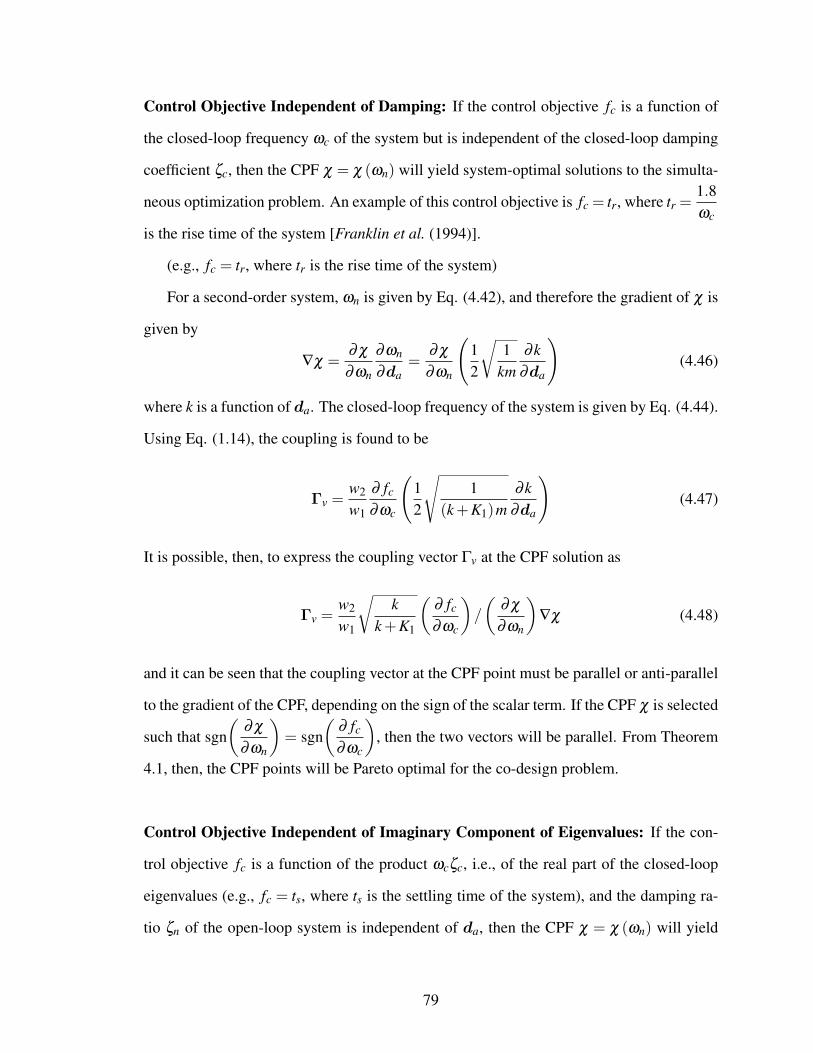
Control Objective Independent of Damping: If the control objective fc is a function of
the closed-loop frequency ωc of the system but is independent of the closed-loop damping
coefficient ζc, then the CPF χ = χ (ωn) will yield system-optimal solutions to the simulta-
neous optimization problem. An example of this control objective is fc = tr, where tr =1.8ωc
is the rise time of the system [Franklin et al. (1994)].
(e.g., fc = tr, where tr is the rise time of the system)
For a second-order system, ωn is given by Eq. (4.42), and therefore the gradient of χ is
given by
∇χ =∂ χ
∂ωn
∂ωn
∂da=
∂ χ
∂ωn
(12
√1
km∂k
∂da
)(4.46)
where k is a function of da. The closed-loop frequency of the system is given by Eq. (4.44).
Using Eq. (1.14), the coupling is found to be
Γv =w2
w1
∂ fc
∂ωc
(12
√1
(k +K1)m∂k
∂da
)(4.47)
It is possible, then, to express the coupling vector Γv at the CPF solution as
Γv =w2
w1
√k
k +K1
(∂ fc
∂ωc
)/
(∂ χ
∂ωn
)∇χ (4.48)
and it can be seen that the coupling vector at the CPF point must be parallel or anti-parallel
to the gradient of the CPF, depending on the sign of the scalar term. If the CPF χ is selected
such that sgn(
∂ χ
∂ωn
)= sgn
(∂ fc
∂ωc
), then the two vectors will be parallel. From Theorem
4.1, then, the CPF points will be Pareto optimal for the co-design problem.
Control Objective Independent of Imaginary Component of Eigenvalues: If the con-
trol objective fc is a function of the product ωcζc, i.e., of the real part of the closed-loop
eigenvalues (e.g., fc = ts, where ts is the settling time of the system), and the damping ra-
tio ζn of the open-loop system is independent of da, then the CPF χ = χ (ωn) will yield
79

system-optimal solutions to the simultaneous optimization problem.
The condition that the damping ratio of the open-loop system is independent of da can
be expressed mathematically as∂ζn
∂da= 0. (4.49)
The gradient ∇χ is, once again, given by Eq. (4.46). Using Eq. (4.44) - (4.45), Γv is
computed from Eq. (1.14) as
Γv =w2
w1
∂ fc
∂ (ωcζc)
(ζc
∂ωc
∂da+ωc
∂ζc
∂da
)(4.50)
By differentiating Eq. (4.43) and substituting Eq. (4.49), it is found that
Γv =w2
w1
∂ fc
∂ (ωcζc)b
4km∂k
∂da(4.51)
and therefore the coupling vector can be expressed in terms of the gradient ∇χ as
Γv =w2
w1
∂ fc
∂ (ωcζc)b
2√
km
(1/
∂ χ
∂ωn
)∇χ (4.52)
and it can again be seen that the coupling vector at the CPF point must be parallel or anti-
parallel to the gradient of the Control Proxy Function, depending on the sign of the scalar
term. If the open-loop system is stable, b > 0, and the function χ should be chosen such
that sgn(
∂ χ
∂da
)= sgn
(∂ fc
∂ (ωcζc)
). If this condition is met, then the two vectors will be
parallel. From Theorem 4.1, then, the CPF points will be Pareto optimal for the co-design
problem.
Damping Term b Independent of da: If the controller objective fc is an arbitrary func-
tion of the closed-loop eigenvalues of the system, and the damping term b in the system
80
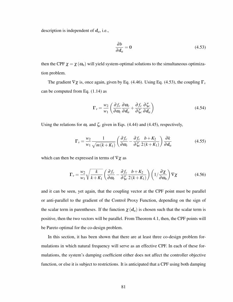
description is independent of da, i.e.,
∂b∂da
= 0 (4.53)
then the CPF χ = χ (ωn) will yield system-optimal solutions to the simultaneous optimiza-
tion problem.
The gradient ∇χ is, once again, given by Eq. (4.46). Using Eq. (4.53), the coupling Γv
can be computed from Eq. (1.14) as
Γv =w2
w1
(∂ fc
∂ωc
∂ωc
∂da+
∂ fc
∂ζc
∂ζc
∂da
)(4.54)
Using the relations for ωc and ζc given in Eqs. (4.44) and (4.45), respectively,
Γv =w2
w1
1√m(k +K1)
(∂ fc
∂ωc− ∂ fc
∂ζc
b+K2
2(k +K1)
)∂k
∂da(4.55)
which can then be expressed in terms of ∇χ as
Γv =w2
w1
√k
k +K1
(∂ fc
∂ωc− ∂ fc
∂ζc
b+K2
2(k +K1)
)(1/
∂ χ
∂ωn
)∇χ (4.56)
and it can be seen, yet again, that the coupling vector at the CPF point must be parallel
or anti-parallel to the gradient of the Control Proxy Function, depending on the sign of
the scalar term in parentheses. If the function χ (da) is chosen such that the scalar term is
positive, then the two vectors will be parallel. From Theorem 4.1, then, the CPF points will
be Pareto optimal for the co-design problem.
In this section, it has been shown that there are at least three co-design problem for-
mulations in which natural frequency will serve as an effective CPF. In each of these for-
mulations, the system’s damping coefficient either does not affect the controller objective
function, or else it is subject to restrictions. It is anticipated that a CPF using both damping
81

of the open-loop system and the natural frequency would be effective in some additional
cases, where these restrictions are not satisfied. Furthermore, all three of these problem for-
mulations require the system to be modeled by second-order dynamics. It is expected that
these results for a CPF using natural frequencies could be extended to systems of higher
order. It is also conjectured that a CPF based on open-loop eigenvalues would be valid with
some types of constraints, and it is anticipated that future research will develop such CPFs.
However, a CPF using open-loop eigenvalues will not be effective when the matrix B
is sensitive to the artifact design variables da, since open-loop eigenvalues cannot be used
to model that system behavior. For problems of this type, the CPF must be based on some
other fundamental metric of the system which is capable of modeling both the free and
forced response characteristics of the system. The next section will evaluate the use of the
controllability Grammian matrix Wc, which depends on both the A and B matrices, for
problems where the derivatives of the B matrix with respect to some components of da,∂B
∂dai
, are significant.
4.3.2 Control Proxy Functions Based on the Controllability Grammian
As shown in the previous section, a CPF based on natural frequency can be effective
for problems in which the matrix B in Eq. (4.36) is not a function of the artifact design
variables, da. If B is a function of da, then the CPF must incorporate B in some way.
Since the controllability Grammian matrix Wc incorporates both the free and forced re-
sponse characteristics of a system, it is logical to consider its use in a CPF. Furthermore,
the physical meaning of the controllability Grammian matrix suggests that it might be ef-
fective as a CPF. The control effort required to move a system from one state to another is
a function of the controllability Grammian matrix. If the determinant of the controllability
Grammian matrices are compared for two systems, the system with the larger determinant
will require less control effort for the same state transition; or, alternatively, the system
with the larger determinant can be moved farther or faster with the same control effort. It
82

is therefore evident that the controllability Grammian matrix can be used to predispose a
system to effective control, and may often be a good choice of CPF. This section will exam-
ine situations in which a CPF based on either the time-dependent controllability Grammian
matrix, Wc(t f), or the steady-state controllability Grammian matrix, W∞
c , is perfect. In
all cases, it is assumed that:
1. The co-design problem is formulated as in Eq. (1.9)-(1.13).
2. The system dynamics are linear and can be described in state-space form as in Eq.
(4.36).
Control Proxy Function for the Case of Control Effort as Objective
Consider the case in which the control objective is to minimize control effort, as de-
scribed in Eq. (3.9). If an optimal controller is chosen, then as stated in Chapter III, the
control objective function fc can be found from Eq. (3.10) to be
fc = xTfW
−1c x f . (4.57)
This expression for fc depends only on da, and thus could serve as a CPF. Since the cou-
pling vector Γv was calculated from this relation, as in Eq. (3.12), it can easily be seen that,
for χ (da) = xTfW
−1c x f ,
Γv =wc
wa∇χ (4.58)
and thus, the CPF is perfect.
There are situations, however, when a simpler CPF would suffice. In Case Ia, as detailed
in Chapter III, the final state of the system, x f , is a parameter. Logically, one might expect
that when this is the case, a CPF based only on Wc may be effective, and in at least two
situations this is true, as shown below.
83

Consider first the case where the components of x f are equal, i.e., x fq = α ∀ q =
1, . . . , p. In this case, a CPF of
χ (da) =p
∑q=1
p
∑t=1
W−1c (q, t) (4.59)
is chosen. It is shown here that this will be a perfect CPF.
The gradient of Eq. (4.59) is given by
∇χ =
∑pq=1 ∑
pt=1 ∂W−1
c (q, t)
∂da1
∑pq=1 ∑
pt=1 ∂W−1
c (q, t)
∂da2...
∑pq=1 ∑
pt=1 ∂W−1
c (q, t)
∂dan
T
(4.60)
The coupling vector Γv is found from Eq. (3.13):
Γv =wc
wa
∑pq=1 ∑
pt=1 x fqx ft
∂W−1c (q, t)∂da1
∑pq=1 ∑
pt=1 x fqx ft
∂W−1c (q, t)∂da2
...
∑pq=1 ∑
pt=1 x fqx ft
∂W−1c (q, t)∂dan
T
(4.61)
which can be re-written as
Γv =wc
wa
α2∂ ∑
pq=1 ∑
pt=1W
−1c (q, t)
∂da1
α2∂ ∑
pq=1 ∑
pt=1W
−1c (q, t)
∂da2...
α2∂ ∑
pq=1 ∑
pt=1W
−1c (q, t)
∂dan
T
(4.62)
84

Thus,
Γv =wc
waα
2∇χ (4.63)
and, as stated, Eq. (4.59) will be a perfect CPF. Note that, if Wc(t f)
is diagonal, the CPF
can be expressed as
χ (da) = tr(W−1
c)
=tr(Wc)
det(Wc)(4.64)
In general, Wc(t f)
is not diagonal. However, if the system’s balanced realization is used,
then Wc(t f)
will be diagonal, regardless of the value of t f [Kailath (1980)]. This is there-
fore recommended, as it simplifies the expression for χ .
In contrast, consider a situation in which the parameter x f has as its only non-zero
component the jth element, i.e., x f j 6= 0, x fq = 0 ∀ q 6= j; this situation corresponds to
problems in which a system is to be moved to a final location where it is at rest. A CPF of
χ =W−1c j j
(t f)
=W ∗
c j j
(t f)
det(Wc)(4.65)
is chosen, where W ∗c(t f)
is the adjoint matrix of Wc(t f), and W ∗
c j j
(t f)
is the ( j j)th
element of W ∗c(t f). Note that, if the ( j j)th element of W ∗
c(t f)
is not a function of da,
then this is equivalent to maximizing the determinant ofWc(t f). It will be shown here that
this is a perfect CPF.
The gradient of Eq. (4.59) is given by
∇χ =
∂W−1c j j
(t f)
∂da1∂W−1
c j j
(t f)
∂da2...
∂W−1c j j
(t f)
∂dan
T
(4.66)
85
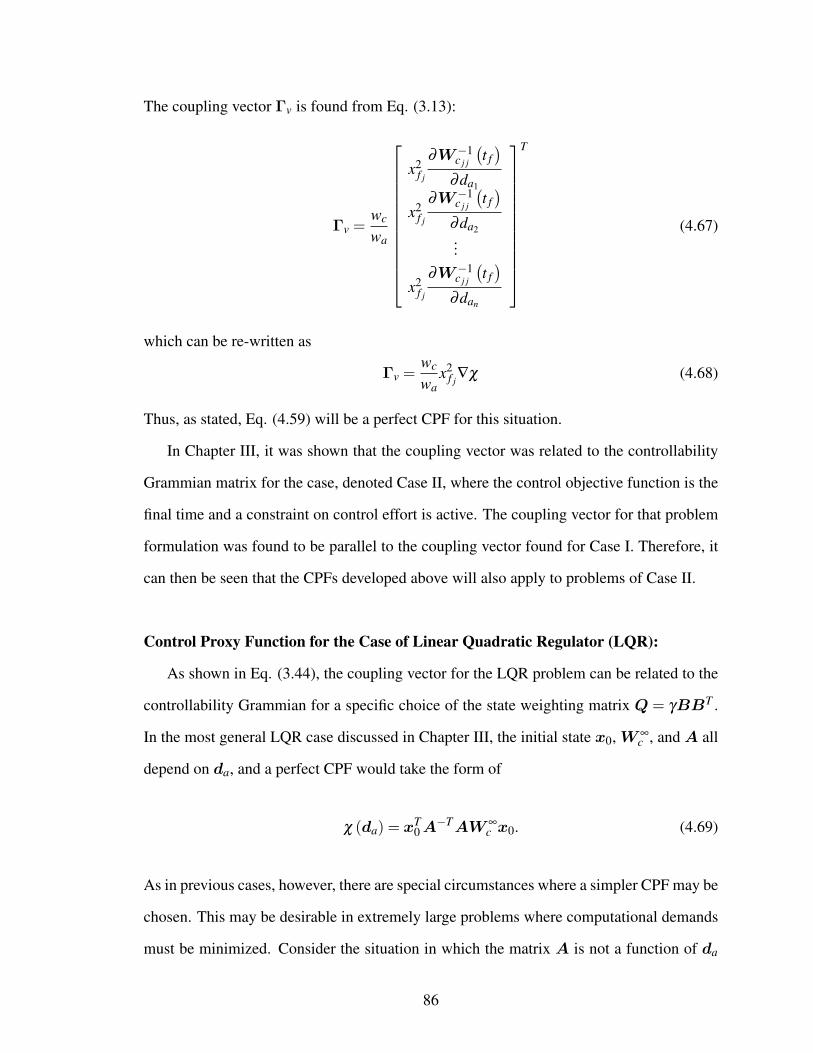
The coupling vector Γv is found from Eq. (3.13):
Γv =wc
wa
x2f j
∂W−1c j j
(t f)
∂da1
x2f j
∂W−1c j j
(t f)
∂da2...
x2f j
∂W−1c j j
(t f)
∂dan
T
(4.67)
which can be re-written as
Γv =wc
wax2
f j∇χ (4.68)
Thus, as stated, Eq. (4.59) will be a perfect CPF for this situation.
In Chapter III, it was shown that the coupling vector was related to the controllability
Grammian matrix for the case, denoted Case II, where the control objective function is the
final time and a constraint on control effort is active. The coupling vector for that problem
formulation was found to be parallel to the coupling vector found for Case I. Therefore, it
can then be seen that the CPFs developed above will also apply to problems of Case II.
Control Proxy Function for the Case of Linear Quadratic Regulator (LQR):
As shown in Eq. (3.44), the coupling vector for the LQR problem can be related to the
controllability Grammian for a specific choice of the state weighting matrix Q = γBBT .
In the most general LQR case discussed in Chapter III, the initial state x0, W∞c , and A all
depend on da, and a perfect CPF would take the form of
χ (da) = xT0A−TAW∞
c x0. (4.69)
As in previous cases, however, there are special circumstances where a simpler CPF may be
chosen. This may be desirable in extremely large problems where computational demands
must be minimized. Consider the situation in which the matrix A is not a function of da
86

and the initial state x0 is a parameter with exactly one non-zero component, i.e., x0 j 6= 0,
x0q = 0 ∀ q 6= j,0 ≤ q ≤ p. Furthermore, the matrix W∞c is diagonal, which will be the
case when a balanced realization is utilized.
For the system described above, select a CPF of
χ (da) =W∞c j j
. (4.70)
The gradient of Eq. 4.70 is given by
∇χ =
∂W∞c j j
∂da1∂W∞
c j j
∂da2...
∂W∞c j j
∂dan
T
(4.71)
The coupling vector can be computed from Eq. (3.45) and is given by the relation
Γv =wc
waγ
1detA
x20 j
A2j j
∂W ∞c j j
∂da1
1detA
x20 j
A2j j
∂W ∞c j j
∂da2...
1detA
x20 j
A2j j
∂W ∞c j j
∂dan
T
(4.72)
This leads to the relation
Γv =wc
wa
γ
detAx2
0 jA2
j j∇χ (4.73)
and therefore the CPF is perfect for this problem.
In this section, it has been shown that a CPF based on the controllability Grammian ma-
trix,Wc(t f), can be effective for many problems in which either fc or an active constraint
is dependent on control effort. This includes some problems in which the control objective,
87

fc, is the response time of the system. For the specific problem formulations investigated
here, a perfect CPF can be formulated based on either the the time-dependent or steady-
state controllability Grammian matrix. As previously stated, these problem formulations
are not exhaustive. It is anticipated that future work will show that a CPF based on the
controllability Grammian matrix will be effective for additional co-design problem formu-
lations, particularly those in which the objective function or constraints are dependent on
control effort.
However, it may not always be possible to formulate a perfect CPF based on the control
Grammian. For example, consider the case where fc is the maximum control signal, rather
than control effort. A control signal with a high peak that quickly decays may result in a
lower control effort than a signal with a lower peak that does not decay as quickly. The
relationship between the maximum control signal and control effort, and the choice of an
appropriate CPF for problems in which the control objective, fc, is based on the maximum
control signal, requires further investigation. It is conjectured that a CPF based on the con-
trollability Grammian will produce results that are near-optimal for a variety of problems,
since it provides a measure of how easily a system is controlled.
4.4 Summary
In this chapter, a new method of solution for co-design problems was introduced, based
upon a sequential optimization using a Control Proxy Function (CPF). The intent of the
CPF method is to provide solutions that are identical with, or close to, the Pareto optimal
solutions to the co-design problem, while allowing the problem to be decomposed into an
artifact design problem and a control design problem. This decomposition allows the co-
design problem to be more easily formulated and solved by experts in each of the functional
areas of artifact design and control design. The key to the effectiveness of this method is
the choice of the CPF. Therefore, guidelines to choose a CPF and a metric to evaluate the
closeness of the solutions have been developed and presented in this chapter. Furthermore,
88

CPFs based on natural frequency and on the controllability Grammian matrix have been de-
veloped for specific problem formulations. These CPFs are all based on the assumption that
the system of interest is linear and time-invariant. For a CPF based on natural frequency,
the system is also assumed to be second-order, though this assumption does not apply to
the use of the controllability Grammian matrix. The CPFs developed in this chapter are not
exhaustive; it is possible to formulate and evaluate additional CPFs, based on open-loop
eigenvalues, the controllability Grammian, and possibly other system metrics. CPFs for
systems that are non-linear or which are not time-invariant could be developed, since the
development of the mathematical basis for the use of a CPF did not require these assump-
tions. Of course, with a variety of possible CPFs, it is important to be able to determine
easily which, if any, will be effective for a given system. If a CPF were found only by trial
and error, or if the selection of a CPF were to require complex calculations, then the method
would offer few advantages over other available solution techniques. In the next chapter, a
set of tests will be given to determine whether a particular problem could be solved with a
CPF, and if so, which CPF should be chosen. The selection of an appropriate CPF will be
demonstrated by means of an example, and the computational effort required to solve the
problem by the CPF method versus the simultaneous method will be discussed.
89

CHAPTER V
Application of the CPF Method
5.1 Introduction
In Chapter IV, the Control Proxy Function (CPF) method was developed and presented.
This method allows a designer to perform sequential optimization of a coupled co-design
problem, while producing optimal or near-optimal results. The CPF method offers sev-
eral advantages over other methods of optimizing co-design problems, including reduced
computational complexity and the ability to optimize the artifact before the controller con-
figuration has been defined. However, in order to take advantage of the CPF method, it is
necessary to easily identify or formulate an appropriate CPF. If it were intrinsically diffi-
cult to formulate the CPF problem, then it would not be useful in practice. Likewise, if the
formulation of the CPF problem were to require highly specialized knowledge or expertise,
its utility would be limited. Therefore, in this chapter we will present a simple procedure
which a designer can use to determine whether she should consider using the CPF problem
formulation, and if so, criteria to determine the type of CPF to be used.
An overview of the CPF selection process will be given in Section 5.2. In Section
5.3, the mathematical model of a MEMS actuator and its controller will be developed
and presented. Two different co-design problems for the MEMS actuator will then be
formulated and solved in Sections 5.4 and 5.5, using the approach presented in Section 5.2.
In both cases, uni-directional coupling is found to be present, and an appropriate CPF will
90

be chosen for each case. In the first case, a suitable CPF can be formulated based on either
the natural frequency or the controllability Grammian. However, for the second problem
a CPF based on natural frequency is not suitable, while one based on the controllability
Grammian is effective. The actuator model and control architecture will be identical in
both cases, with changes made only to the objectives, constraints, and design variables.
5.2 Overview of Design Process Using a CPF
The process used to decide whether a CPF problem formulation is feasible for a given
co-design problem, shown in Fig. 5.1, is performed as follows:
STEP 1: Problem Formulation
The process begins with the formulation of the co-design problem in the form of Eqs.
(1.9)-(1.13). In this step, the artifact and control objectives, fa and fc, are chosen, the sys-
tem model is developed, artifact and control design variables, da and dc, are chosen, and
artifact and controller inequality and equality constraints, ga, ha, gc, and hc, are formu-
lated.
STEP 2: Evaluation for Bi-Directional Coupling
After problem formulation, the designer evaluates the co-design problem to determine
whether or not bi-directional coupling is present. If the artifact objective function, fa, or
any of the constraints, ga and ha, are functions of any of the control design variables, dc,
then bi-directional coupling exists, based on the definition given in Section 1.3.1. In this
case, the CPF method does not apply, and the optimization should be performed using one
of the methods discussed in Section 1.2.
STEP 3: Evaluation for Uni-Directional Coupling
If the co-design problem does not exhibit bi-directional coupling, then the designer
91

evaluates the problem to determine whether it exhibits uni-directional coupling. This eval-
uation is a two-step process; first, the control objective function, fc, and constraints, gc
and hc, are examined to determine whether they are functions of any of the artifact design
variables, da. If they are not, i.e., if fc = fc (dc), gc = gc (dc), and hc = hc (dc), then the
problem is uncoupled, and should be solved with a simple sequential optimization.
If fc = fc (da,dc), gc = gc (da,dc), or hc =hc (da,dc), the problem may still decouple
under certain conditions. In Chapter III, conditions were presented under which a co-design
problem will decouple. It is, therefore, necessary to check the co-design problem to deter-
mine whether it satisfies any of these decoupling conditions, as discussed in Chapter III (see
Eqs. (3.12), (3.30), (3.44)). If it does satisfy one of these conditions, then the coupling will
vanish, and the problem can be solved using sequential optimization. If the problem does
not satisfy any of the decoupling conditions, then it is considered to exhibit uni-directional
coupling, and the CPF solution method can be considered.
STEP 4: Evaluation of Suitability of CPF Method
Any co-design problem with uni-directional coupling could be formulated as a CPF
problem. However, in order to formulate a CPF problem that is effective at finding optimal
(or near-optimal) solutions, one must be able to specify an appropriate CPF. This can be
done in one of two ways, as indicated in Fig. 5.1. First, the problem may be of a type for
which a CPF has already been developed. In this case, the designer simply has to determine
that the problem is of the appropriate type, and she can use that CPF. The CPFs that were
developed in Chapter IV are listed in Table 5.1, along with the conditions required to use
them. These CPFs and their conditions for use are briefly re-stated in this section. Since
this list is not exhaustive, it is anticipated that more CPFs will be developed, and the range
of problems amenable to solution with existing CPFs will increase.
If a CPF, such as those listed in Table 5.1, has not been developed for a given problem,
then the designer may consider formulating one. If the control objective function fc (da,dc)
92

Figure 5.1: Choice of Solution Method for Co-Design Problems
is clearly monotonic, or is known to have an unconstrained minimum in the da-space, then
it may be possible to use this information to formulate a CPF for the problem based on
Theorems 4.3 and 4.4.
As stated in Chapter IV, all of the CPFs that have been developed assume that the sys-
tem dynamics can be modeled as linear and time-invariant. In the case of a CPF based
on natural frequency, there is an additional assumption that system is second-order. This
93

Table 5.1: Control Proxy Functions (CPFs) and Conditions for Use (See Eqs. (4.38), (4.35),(4.44), (4.45), (4.43), (3.4), and (3.5) for the definitions of B, b, ωc, ζc, ζn,Wc(t f), andW∞
c , respectively.)
Control Proxy Function, χ Conditions for UseCPF Based on Natural Frequency (for second-order dynamics)
χ =1
ωnor χ =−ωn
∂B
∂dai
= 0 ∀ i = 1, . . . ,n
fc = fc (ωc)∂B
∂dai
= 0 ∀ i = 1, . . . ,n
fc = fc (ωcζc)∂ζn
∂da= 0
∂B
∂dai
= 0 ∀ i = 1, . . . ,n
∂b∂da
= 0
CPFs Based on Controllability Grammian Matrix
χ =tr(Wc(t f))
det(Wc(t f))
fc =∫ t f
0 (u(t))2 dt, where t f is a parameterWc(t f)
is diagonalx fi = α ∀ i = 1, . . . ,q, where α is a parameterfc = t f
gc =∫ t f
0 (u(t))2 dt−Emax ≤ 0Wc(t f)
is diagonalx fi = α ∀ i = 1, . . . ,q, where α is a parameter
χ =W ∗c j j
(t f)
det(Wc(t f))
fc =∫ t f
0 (u(t))2 dt, where t f is a parameterWc(t f)
is diagonalx fi = 0 ∀ i = 1, . . . ,q, i 6= j, x f j = α , where α is a parameterfc = t f
gc =∫ t f
0 (u(t))2 dt−Emax ≤ 0Wc(t f)
is diagonalx fi = 0 ∀ i = 1, . . . ,q, i 6= j, x f j = α , where α is a parameter
χ =W∞c j j
LQR control is to be appliedA 6=A(da)x0i = 0 ∀ i = 1, . . . ,q, i 6= j, x0 j = α , where α is a parameterW∞
c is diagonal
94

assumption is not made for CPFs based on the controllability Grammian, which apply to
systems of arbitrary order. The CPFs derived in Chapter IV and given in Table 5.1 are
briefly summarized here.
CPF Based on Natural Frequency
As shown in Chapter IV, a CPF based on natural frequency can be effective in some
cases. Here, three sets of conditions are presented in which this type of CPF is appropriate.
If any of the three sets of conditions in Table 5.1 is satisfied, then a CPF of either χ =1
ωn
or χ = −ωn will provide Pareto optimal solutions to the co-design problem. If any set of
conditions is ‘almost’ satisfied, then a CPF based on natural frequency can be expected to
yield solutions that are near-optimal.
The first set of conditions under which natural frequency is appropriate is the case where
the matrix B, as defined in Eq. (4.36), is invariant with respect to the design variables da
and the control objective function depends only on the frequency of the controlled system,
ωc. In this situation, the free response of the system is dependent on da, but the forced
response is invariant with da. One example of this type of objective would be the rise time
of a system, which is given by the relation tr =1.8ωc
.
In the second set of conditions under which natural frequency is appropriate, the matrix
B and the damping of the uncontrolled system, ζn, are invariant with respect to the design
variables da, and the objective function fc is a function of the real part of the eigenvalues
of the controlled system. One example of this type of objective would be the settling time
of a system, which is given by the relation ts =4
ζcωc.
In the third set of conditions for the use of natural frequency as a CPF, the matrix B
and the damping term b of the differential equation given by Eq. (4.35), are invariant with
respect to the design variables da. In this situation, the control objective can be an arbitrary
function of the controlled system frequency and damping, ωc and ζc.
95

CPF Based on Controllability Grammian Matrix
Three distinct CPFs are presented in Table 5.1 based on the controllability Grammian
matrix. Two of those CPFs are valid for more than one set of conditions, while the third
CPF is only valid for one set of conditions. They are briefly summarized here.
A CPF based on the trace and determinant of the time-dependent controllability ma-
trix, χ =tr(Wc(t f))
det(Wc(t f)) , can be used in either of two sets of conditions. In both sets of
conditions, the matrixWc(t f)
is diagonal, which will occur when the balanced realization
is used. Also in both cases, the final state for the system is a parameter for which all of
its components are equal. This can occur when the states comprising the vector x f are all
positions, and every component of the system is to be moved to the same position. The
difference between the two sets of conditions for this CPF is seen in the role of the control
effort; in one set of conditions, the control objective function is the control effort, while
the other set of conditions is based on a constraint on the control effort. In that case, the
control objective is the final time at which the system reaches the state x f .
A CPF based on a single value of the adjoint matrix, W ∗c(t f), and on the determinant
of the time-dependent controllability Grammian matrix, Wc(t f), is formulated as χ =
W ∗c j j
det(Wc(t f)) . This CPF is also valid under two separate sets of circumstances. In both
sets of conditions, the matrix Wc(t f)
is diagonal. Also in both cases, the final state of the
system is a parameter, where only one component of x f is non-zero. As an example of
this situation, consider the case where a system is to be moved to a specified location, at
which it is to be at rest. The location of the system is given by the non-zero component of
x f , while the remaining components represent velocities, which must be zero. Again, the
difference between the two sets of conditions for this CPF is seen in the role of the control
effort; in one set of conditions, the control objective function is the control effort, while
the other set of conditions is based on a constraint on the control effort. In that case, the
control objective is the final time at which the system reaches the state x f .
The final CPF developed in Chapter IV and given in Table 5.1 is valid only under one
96
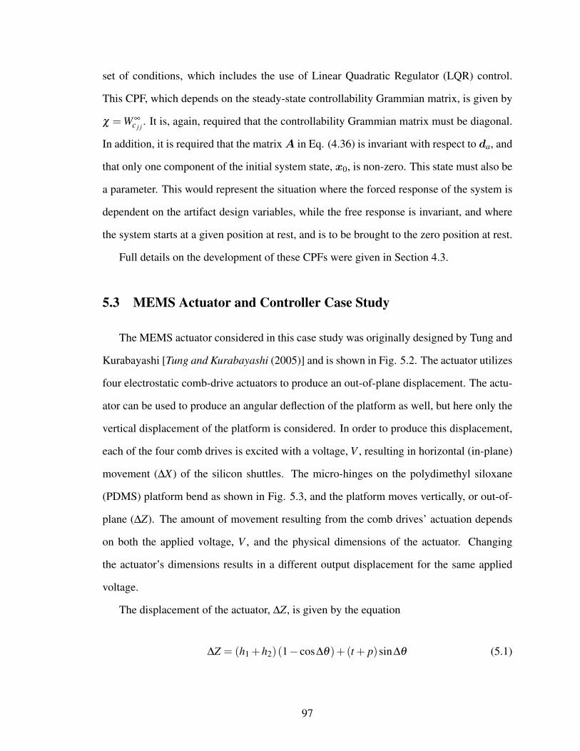
set of conditions, which includes the use of Linear Quadratic Regulator (LQR) control.
This CPF, which depends on the steady-state controllability Grammian matrix, is given by
χ = W ∞c j j
. It is, again, required that the controllability Grammian matrix must be diagonal.
In addition, it is required that the matrixA in Eq. (4.36) is invariant with respect to da, and
that only one component of the initial system state, x0, is non-zero. This state must also be
a parameter. This would represent the situation where the forced response of the system is
dependent on the artifact design variables, while the free response is invariant, and where
the system starts at a given position at rest, and is to be brought to the zero position at rest.
Full details on the development of these CPFs were given in Section 4.3.
5.3 MEMS Actuator and Controller Case Study
The MEMS actuator considered in this case study was originally designed by Tung and
Kurabayashi [Tung and Kurabayashi (2005)] and is shown in Fig. 5.2. The actuator utilizes
four electrostatic comb-drive actuators to produce an out-of-plane displacement. The actu-
ator can be used to produce an angular deflection of the platform as well, but here only the
vertical displacement of the platform is considered. In order to produce this displacement,
each of the four comb drives is excited with a voltage, V , resulting in horizontal (in-plane)
movement (∆X) of the silicon shuttles. The micro-hinges on the polydimethyl siloxane
(PDMS) platform bend as shown in Fig. 5.3, and the platform moves vertically, or out-of-
plane (∆Z). The amount of movement resulting from the comb drives’ actuation depends
on both the applied voltage, V , and the physical dimensions of the actuator. Changing
the actuator’s dimensions results in a different output displacement for the same applied
voltage.
The displacement of the actuator, ∆Z, is given by the equation
∆Z = (h1 +h2)(1− cos∆θ)+(t + p)sin∆θ (5.1)
97
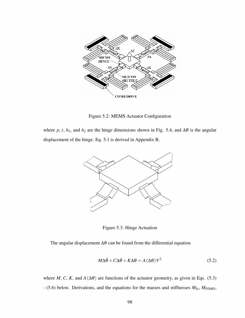
Figure 5.2: MEMS Actuator Configuration
where p, t, h1, and h2 are the hinge dimensions shown in Fig. 5.4, and ∆θ is the angular
displacement of the hinge. Eq. 5.1 is derived in Appendix B.
Figure 5.3: Hinge Actuation
The angular displacement ∆θ can be found from the differential equation
M∆θ +C∆θ +K∆θ = A(∆θ)V 2 (5.2)
where M, C, K, and A(∆θ) are functions of the actuator geometry, as given in Eqs. (5.3)
- (5.6) below. Derivations, and the equations for the masses and stiffnesses MSi, MPDMS,
98

Figure 5.4: Micro-Hinge Structure
Mhinge, KSi, and KPDMS, are given in [Tung and Kurabayashi (2005)] and in Appendix B.
M = MSi (h1 +h2)2 +MPDMS (t + p)2 +
13
Mhinge
((h1 +h2)
2 +(t + p)2)
(5.3)
C = 2ζ
√(MSi (h1 +h2)
2 +MPDMS (t + p)2)(
KSi (h1 +h2)2 +2KPDMS
)(5.4)
K = KSi (h1 +h2)2 +2KPDMS (5.5)
A(∆θ) =nεo (h1 +h2)
d((h1 +h2)− (t + p)∆θ) (5.6)
where ζ is an experimentally determined parameter, n is the number of fingers in the comb
drive, εo is the permittivity of vacuum, and d is the width of a finger, as shown in Fig. 5.5.
Alternatively, the system dynamics may be written in state-space form as
∆θ
∆θ
=
0 1
−K/M −C/M
∆θ
∆θ
+
0
A(∆θ)/M
V 2 (5.7)
An integral controller with state feedback is applied to the system, as shown in Fig. 5.6.
It is assumed that the angle ∆θ and the angular velocity ∆θ can be measured, and that the
angle ∆θ is to be controlled. The dynamics of the closed-loop system can then be written
99

Figure 5.5: Plan View of Silicon Shuttle
as
M∆θ +(C +K2A(∆θ))∆θ +(K +K1A(∆θ))∆θ −KiA(∆θ)t∫
0
(∆θr−∆θ)dτ (5.8)
Note that the controller output is u =V 2, and that the coefficient A in Eq. (5.2) is a function
of ∆θ . Thus, the resulting controller design problem is non-linear.
Figure 5.6: Control Architecture and System Dynamics
100

5.4 Co-Design of MEMS Actuator for Steady-State Displacement and
Settling Time
Using the system described above, one can follow the procedure outlined in Fig. 5.1 to
formulate a co-design optimization problem and choose an appropriate method of solution.
STEP 1: Problem Formulation
In this problem formulation, the goal is to maximize the steady-state displacement of
the actuator, ∆Zss, and minimize the 1% settling time, ts, as given in Eqs. (5.9) - (5.10). The
artifact constraints, given by Eqs. (5.11) - (5.16), are based on manufacturability, stress,
kinematics, and mechanical and electrical stability. Detailed derivations of the relevant
equations are given in Appendix B. The control constraints, given by Eqs. (5.21) - (5.22),
are formulated to limit the overshoot, Mp, and the maximum voltage, Vmax. The control ob-
jective function and constraints are calculated by numerical integration and implemented in
a Simulink model. The artifact design variables, da, are selected to be the hinge dimensions
p, t, h1, and h2, as shown in Fig. 5.4. These artifact design variables are given the bounds
in Eqs. (5.17) - (5.20). The control design variables are the gains K1, K2, and Ki.
fa = −∆Zss (5.9)
fc = ts (5.10)
ga1 = t−5h1 ≤ 0 (5.11)
ga2 = 910− l1−lp
2−2t +
∆Xss
2≤ 0 (5.12)
ga3 =nεo (h1 +h2)V 2
ssd
− kbπ2EPDMSw(2h1 +h2)3
12p2 ≤ 0 (5.13)
101

ga4 = ∆Xss−(
lSi√2−
l fo
2
)≤ 0 (5.14)
ga5 =EPDMSh1∆θss
2p−σPDMSmax ≤ 0 (5.15)
ga6 =3∆XssESib
4l2Si
−σSimax ≤ 0 (5.16)
where lp is the length of the platform, kb is the beam end condition coefficient, EPDMS is
Young’s modulus for PDMS, lSi is the length of the silicon springs, l f o is the initial finger
engagement, ESi is Young’s modulus for silicon, and σPDMSmax and σSimax are maximum
allowable stresses in PDMS and silicon, respectively.
1 µm ≤ p ≤ 1000 µm (5.17)
1 µm ≤ t ≤ 1000 µm (5.18)
6 µm ≤ h1 ≤ 1000 µm (5.19)
6 µm ≤ h2 ≤ 1000 µm (5.20)
gc1 = Mp−0.05≤ 0 (5.21)
gc2 = Vmax−25≤ 0 (5.22)
All other dimensions and physical properties of the actuator are parameters; in addition,
the steady-state voltage, Vss, is a parameter. Values of the parameters are given in Table 5.2.
STEP 2: Evaluation for Bi-Directional Coupling
The problem can be evaluated to determine whether bi-directional coupling is present.
The functions fa and ga (see Eqs. (5.9) and (5.11) - (5.16)) are not dependent on the control
design variables (i.e., K1, K2, Ki). Therefore, bi-directional coupling does not exist. Note,
102

Table 5.2: Parameter Values for MEMS Actuator
Parameter Valueεo 8.854e-12 F/m
EPDMS 750 KPaESi 190 GPa
ρPDMS 1.05 g/cm3
ρSi 2.44 g/cm3
σSimax 1.5 GPaσPDMSmax 2.24 MPa
n 50d 3 µmb 3 µmlSi 500 µmlp 350 µml f 50 µml1 700 µml2 70 µml3 75 µml4 50 µmw 100 µmζ 0.1
103

Table 5.3: Original Design of MEMS Actuator [Tung and Kurabayashi (2005)]
Variable Value (µm)p 80t 20
h1 20h2 30
however, that an alternative problem formulation in which Vss was not fixed as a parameter
would exhibit bi-directional coupling.
STEP 3: Evaluation for Uni-Directional Coupling
Next, the problem is evaluated to determine whether uni-directional coupling exists.
While explicit relations for fc (see Eq. (5.10)) and gc (see Eq. (5.21) - (5.22)) are not
given, it is clear that the simulation which calculates them depends on M, C, K, and A(∆θ),
and through them, on the artifact design variables, da. Therefore, fc = fc (da,dc) and
gc = gc (da,dc).
The problem is then examined to determine whether or not any of the decoupling con-
ditions in Chapter III, as given by Eqs. (3.12), (3.30), and (3.44), are applicable. This prob-
lem formulation does not match the formulations in any of Cases I, II, or III, and therefore
these conditions do not apply. Thus, the problem is presumed to exhibit uni-directional
coupling, and is a candidate for solution with the CPF method.
STEP 4: Evaluation of Suitability of CPF Method
Now, consider whether one of the CPFs listed in Table 5.1 would be effective in solving
this problem. Begin this evaluation by noting that the MEMS actuator is modeled as a
second-order system. Since this is one of the necessary conditions for the use of natural
frequency, one can consider whether natural frequency will be an effective CPF.
For this problem, the matrix B for the state-space formulation described in Eq. (4.36)
104

is given by
B =
0
A(∆θ)/M
(5.23)
and its derivatives relative to the artifact design variables are given by Eq. (5.24) - (5.27).
These derivatives are evaluated at the values of p, t, h1, and h2 given in Table 5.3, corre-
sponding to the original design [Tung and Kurabayashi (2005)]. This point is used because
it is known to be a feasible design.
∂B
∂ p=
0
46
(5.24)
∂B
∂ t=
0
46
(5.25)
∂B
∂h1=
0
−42
(5.26)
∂B
∂h2=
0
20
(5.27)
It is obvious that the values in Eqs. (5.24) - (5.27) are non-zero. However, if they are
small, then it may be reasonable to regard them as negligible. This raises the question of
what constitutes ‘small’ in a given problem. As an example, it is possible to change the
values of these derivatives by orders of magnitude simply by scaling the problem. There-
fore, some standard of comparison must be used to determine whether the derivatives of
the matrix B are negligible. In order to determine whether they can be considered small,
the derivatives of the matrix A are computed for the state-space formulation described in
105

Eq. (4.36), which is given by
A=
0 1
−K/M −C/M
(5.28)
These derivatives are also evaluated at the values in Table 5.3, and are given in Eqs.
(5.29) - (5.32).
∂A
∂ p=
0 0
3.5e6 6.8e4
(5.29)
∂A
∂ t=
0 0
5.0e6 4.2e4
(5.30)
∂A
∂h1=
0 0
−1.6e7 8.4e5
(5.31)
∂A
∂h2=
0 0
−2.3e6 4.8e5
(5.32)
The values of∂B
∂dai
are several orders of magnitude smaller than∂A
∂dai
. Therefore, it will be
assumed that they are negligible, and the possible use of natural frequency as a CPF will
be further evaluated.
The control objective function, fc = ts =4.6
ζcωc, as given in Eq. (5.10), is a function of
the product ζcωc, which is among the second set of conditions for use of natural frequency
as a CPF. Therefore, the derivatives of the open-loop damping are evaluated to determine
whether or not this set of conditions is satisfied.
The derivatives of the open-loop damping coefficient, ζn, are calculated for each of the
106

artifact design variables, and found to be
∂ζn
∂ p= −1.3e−5 (5.33)
∂ζn
∂ t= −7.0e−6 (5.34)
∂ζn
∂h1= −2.3e−5 (5.35)
∂ζn
∂h2= −8.0e−6 (5.36)
where the artifact design variables p, t, h1, and h2 are measured in microns. The values of
these derivatives may be considered negligible, and therefore the system closely approxi-
mates the second set of conditions for use of natural frequency as a CPF, as described in
Table 5.1. Based on this analysis, then, the co-design problem will be formulated as a CPF
problem utilizing the natural frequency of the system.
5.4.1 Optimization Using Natural Frequency
As stated in Section 4.1, there are a number of different ways to approach bi-objective
optimization problems. One simple approach is to treat one objective as a constraint, ex-
ploring the trade-off by varying the constraint bound in a parametric study [Papalambros
and Wilde (2000)]. This approach will be used to formulate the CPF problem, with the
additional constraint given by
ga7 = ωmin−ωn ≤ 0 (5.37)
where
ωn =
√KM
(5.38)
and the minimum allowable frequency, ωmin, will be set based on an operating frequency,
ωo [Peters et al. (2008)].
ωmin = 1.1ωo (5.39)
107

Table 5.4: Sequential Optimization Results Using Natural Frequency
ωo (rad/s) p (µm) t (µm) h1 (µm) h2 (µm) K1 K2 Ki ∆Zss (µm) ts (ms)500 599 30 6 53 4.01e5 48.4 1.54e9 6.79 0.568750 400 30 6 51 3.62e5 34.4 1.81e9 4.93 0.470
1000 296 30 6 51 3.02e5 23.7 1.87e9 3.84 0.3871250 234 30 6 52 2.88e5 15.3 2.55e9 3.11 0.2481500 189 30 6 52 3.12e5 13.4 3.39e9 2.57 0.2011750 155 30 6 54 2.87e5 11.2 3.49e9 2.15 0.1822000 126 30 6 54 2.53e5 9.10 3.40e9 1.80 0.1662250 100 30 6 54 2.36e5 8.17 3.41e9 1.50 0.1582500 73 30 6 53 2.17e5 6.76 3.46e9 1.23 0.142
Therefore, the CPF problem will be formulated as
minp,t,h1,h2
fa (5.40)
subject to ga (p, t,h1,h2)≤ 0 (5.41)
where fa =−∆Zss, as given by Eq. (5.9), and the constraints ga are given by Eqs. (5.11) -
(5.16) and (5.37); followed by
minK1,K2,Ki
fc (5.42)
subject to gc ≤ 0 (5.43)
where fc = ts, as given by Eq. (5.10), and the constraints gc are given by Eqs. (5.21) -
(5.22). The optimization is carried out for different values of the minimum frequency, ωmin,
as presented in [Peters et al. (2008)]. The different designs produced by the optimization
are given in Table 5.4.
Once these points have been generated for the CPF problem, it is possible to consider
whether, as expected, they match the Pareto frontier of the co-design problem. The simul-
taneous problem was solved, as detailed in [Peters et al. (2008)]. The objectives fa and
fc were combined using the exponential weighted criteria method, as shown in Eq. (5.44)
108

[Athan (1994)]. This method was used due to the non-convex nature of the Pareto frontier;
as stated in Section 1.5.3, a linear combination of objectives is not appropriate in this case.
However, as shown in Section 2.6.1, the relationships derived in Chapters III and IV are
still valid.
f = (ew1−1)e−∆Zss +(ew2−1)ets (5.44)
The results of the simultaneous optimization problem and of the CPF problem are com-
pared in Fig. 5.7. It can be seen that the CPF problem produces results that are indistin-
guishable from the Pareto frontier, visualized from the Pareto points generated by simulta-
neous optimization.
Figure 5.7: Comparison of CPF Points and Simultaneous Optimization Points forFrequency-Based CPF
Note that the CPF problem formulation is a less computationally intensive method
to solve the problem. The computational cost of a simultaneous optimization formula-
tion is typically higher than a sequential formulation [Balling and Sobieszczanski-Sobieski
(1996)]. This problem provides an example of this. For a typical CPF point, 68 function
109

calls are required for the artifact optimization, and 59 function calls for the control opti-
mization, with only the control optimization involving simulation. By contrast, generation
of a typical point for the simultaneous optimization problem requires 137 function calls
for both problems’ functions, all of which require simulation [Peters et al. (2008)]. The
CPF method, then, requires approximately half as many simulations as the simultaneous
optimization, resulting in a more computationally efficient process.
5.4.2 Optimization Using Controllability Grammian
While the use of natural frequency was clearly effective in this problem, it is important
to note that it is not necessarily the only possible CPF for the problem. Suppose that the
control objective had not yet been formulated when the CPF was chosen, and therefore the
CPF was chosen based only on the knowledge that the system would need to be control-
lable. Instead of constraining the natural frequency, consider the use of a constraint on the
determinant of the steady-state controllability Grammian, i.e.,
ga7 = D−detW∞c ≤ 0 (5.45)
where the value of D is varied to produce a set of designs. Since there is no obvious
means to determine the appropriate value of D, its initial value can be chosen by finding
the controllability Grammian for the initial design, as given in Table 5.3. Then, D can be
varied about that value. The CPF problem is then formulated as
minp,t,h1,h2
fa (5.46)
subject to ga (p, t,h1,h2)≤ 0 (5.47)
where fa =−∆Zss, as given by Eq. (5.9), and the constraints ga are given by Eqs. (5.11) -
(5.16) and (5.45); followed by
110
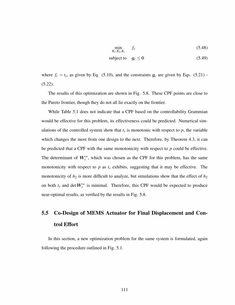
minK1,K2,Ki
fc (5.48)
subject to gc ≤ 0 (5.49)
where fc = ts, as given by Eq. (5.10), and the constraints gc are given by Eqs. (5.21) -
(5.22).
The results of this optimization are shown in Fig. 5.8. These CPF points are close to
the Pareto frontier, though they do not all lie exactly on the frontier.
While Table 5.1 does not indicate that a CPF based on the controllability Grammian
would be effective for this problem, its effectiveness could be predicted. Numerical sim-
ulations of the controlled system show that ts is monotonic with respect to p, the variable
which changes the most from one design to the next. Therefore, by Theorem 4.3, it can
be predicted that a CPF with the same monotonicity with respect to p could be effective.
The determinant of W∞c , which was chosen as the CPF for this problem, has the same
monotonicity with respect to p as ts exhibits, suggesting that it may be effective. The
monotonicity of h2 is more difficult to analyze, but simulations show that the effect of h2
on both ts and detW∞c is minimal. Therefore, this CPF would be expected to produce
near-optimal results, as verified by the results in Fig. 5.8.
5.5 Co-Design of MEMS Actuator for Final Displacement and Con-
trol Effort
In this section, a new optimization problem for the same system is formulated, again
following the procedure outlined in Fig. 5.1.
111
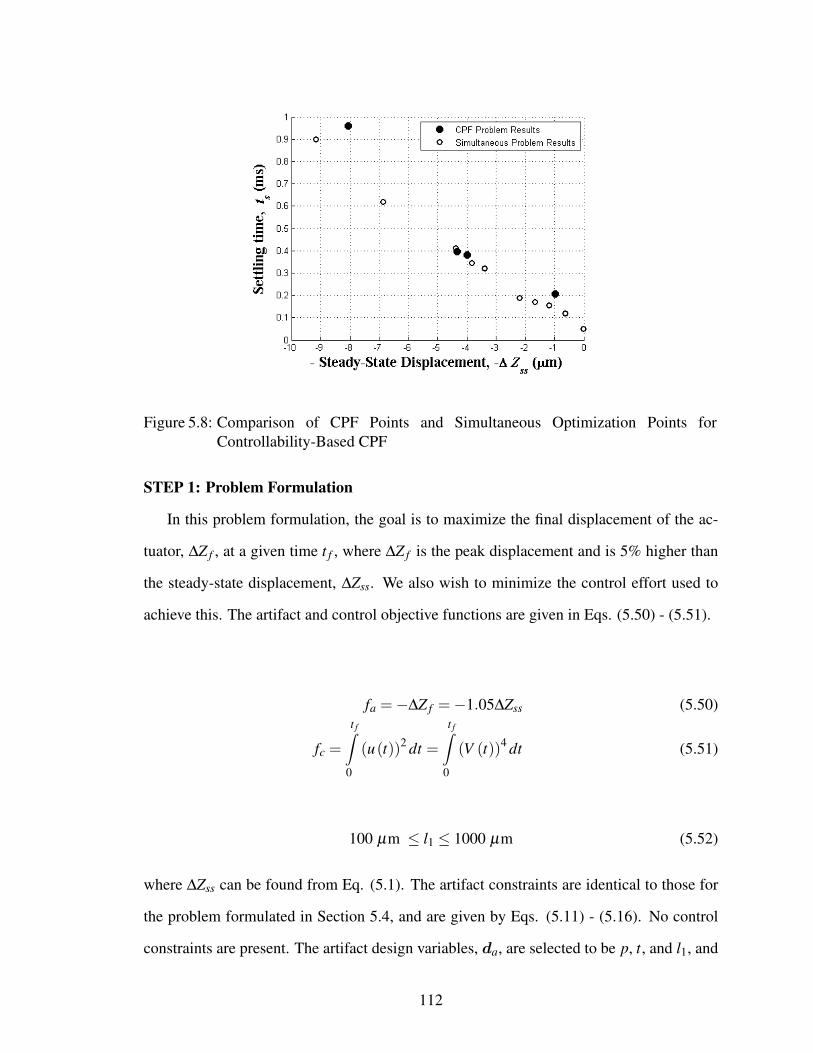
Figure 5.8: Comparison of CPF Points and Simultaneous Optimization Points forControllability-Based CPF
STEP 1: Problem Formulation
In this problem formulation, the goal is to maximize the final displacement of the ac-
tuator, ∆Z f , at a given time t f , where ∆Z f is the peak displacement and is 5% higher than
the steady-state displacement, ∆Zss. We also wish to minimize the control effort used to
achieve this. The artifact and control objective functions are given in Eqs. (5.50) - (5.51).
fa =−∆Z f =−1.05∆Zss (5.50)
fc =
t f∫0
(u(t))2 dt =
t f∫0
(V (t))4 dt (5.51)
100 µm ≤ l1 ≤ 1000 µm (5.52)
where ∆Zss can be found from Eq. (5.1). The artifact constraints are identical to those for
the problem formulated in Section 5.4, and are given by Eqs. (5.11) - (5.16). No control
constraints are present. The artifact design variables, da, are selected to be p, t, and l1, and
112

are given the bounds in Eqs. (5.17), (5.18), and (5.52). The control design variables are,
again, the gains K1, K2, and Ki. Note that the artifact design variable l1 does not appear in
either the artifact objective function, fa, or in the artifact inequality constraints, ga. It is
expected, therefore, that it will either be irrelevant to the co-design problem or will appear
in the control objective function.
The parameters h1 and h2 are assigned the values of 20 µm and 30 µm, respectively,
based on the original design in [Tung and Kurabayashi (2005)]. The final time, t f , is a pa-
rameter and is given as t f = 0.25 ms. This value is chosen based on the system responses
seen in the first optimization. All other parameters have the values given in Table 5.2. Note
that, in the first problem formulation, the primary concern was the speed of response. In
this problem formulation, control effort is to be minimized.
STEP 2: Evaluation for Bi-Directional Coupling
The problem can then be evaluated to determine whether bi-directional coupling is
present. The functions fa and ga are not dependent on the control design variables. There-
fore, bi-directional coupling does not exist.
STEP 3: Evaluation for Uni-Directional Coupling
Next, the problem is evaluated to determine whether uni-directional coupling exists.
While explicit relations for fc and gc are not given, the simulation which calculates them
depends on M, C, K, and A(∆θ), and through them, on the artifact design variables, da.
Therefore, fc = fc (da,dc) and gc = gc (da,dc).
The problem is then evaluated to determine whether or not any of the decoupling con-
ditions in Chapter III (i.e., Eqs. (3.12), (3.30), (3.44)) are applicable. In this case, the
problem does match one of the formulations given in Chapter III, specifically the formu-
lation denoted as Case I. Evaluation of Eq. (3.12) indicates that this co-design problem
is coupled, since the coupling vector will not vanish for any feasible values of the artifact
113

design variables. Therefore, the problem exhibits uni-directional coupling.
STEP 4: Evaluation of Suitability of CPF Method
Now, consider whether one of the CPFs listed in Table 5.1 would be effective in solving
this problem. While the B matrix is insensitive to the design variables, the remaining
conditions are not met for the use of natural frequency as a CPF. The control objective
function, fc, is not a function of only ωc, so the first set of conditions is not satisfied. The
second set of conditions is not satisfied, since fc is not a function of the product ωcζc. The
third set of conditions is not satisfied, since∂b
∂da6= 0. Therefore, the natural frequency is
not an appropriate choice of CPF for this problem.
The system does not satisfy the conditions for use of any of the controllability-based
CPFs listed in Table 5.1. However, one can easily formulate an appropriate CPF for this
problem. Since this problem matches Case I in Chapter III, we know that, for an optimal
controller,
fc = xTfWc
(t f)−1
x f (5.53)
which, for this problem, can be expressed as
fc =∆Z2
fWc22
(t f)
det(Wc(t f)) . (5.54)
Therefore, the CPF χ1 is chosen to be the control objective function, fc, given by Eq.
(5.54).
The characteristics of the Pareto frontier are not known prior to solution of the problem.
Since the convexity of the Pareto frontier is not known, we will consider the possibility that
it may be non-convex, and therefore the bi-objective optimization of fa and χ is formulated
with the exponential weighted criteria function [Athan (1994)]. The CPF problem is given
by
114

Table 5.5: CPF Optimization Results Using χ1
p (µm) t (µm) l1 (µm) K1 K2 Ki ∆Z f (µm) E162 25 523 5.72e5 28.2 6.47e9 2.08 22.82176 25 509 6.60e5 32.4 7.40e9 2.26 25.71188 25 497 7.43e5 36.3 8.28e9 2.42 29.11199 25 486 8.27e5 40.2 9.17e9 2.57 33.17211 25 475 9.14e5 44.3 1.01e10 2.71 38.10222 25 463 1.01e6 48.7 1.11e10 2.85 44.22233 25 452 1.11e6 53.5 1.22e10 3.00 51.00246 25 439 1.22e6 59.0 1.34e10 3.15 59.59259 25 426 1.36e6 65.4 1.49e10 3.32 72.33
minp,t,l1
((e2w1−1
)e2 fa +
(e2w2−1
)e2χ1
)(5.55)
subject to the constraints given in Eqs. (5.11) - (5.16), followed by
minK1,K2,Ki
E (5.56)
where
E =
t f∫0
(V (t))4 dt. (5.57)
Results are given in Table 5.5, and the optimal values of −∆Z f and E are shown in Fig.
5.9. At each of the points shown, the angle ξ is calculated in order to determine whether
the point is optimal or near-optimal. For each point, ξ = 0, indicating that the CPF points
are Pareto optimal, as anticipated.
Again, it should be noted that this CPF is not necessarily the only one that would be
effective for this problem. Consider the case where we ignore the contribution of ∆Z f to
χ1, and use the CPF
χ2 =Wc22
(t f)
det(Wc(t f)) . (5.58)
The results of this optimization, as shown in Fig. 5.10, match the Pareto optimal set found
115
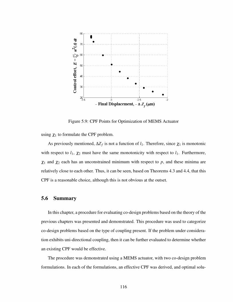
Figure 5.9: CPF Points for Optimization of MEMS Actuator
using χ1 to formulate the CPF problem.
As previously mentioned, ∆Z f is not a function of l1. Therefore, since χ1 is monotonic
with respect to l1, χ2 must have the same monotonicity with respect to l1. Furthermore,
χ1 and χ2 each has an unconstrained minimum with respect to p, and these minima are
relatively close to each other. Thus, it can be seen, based on Theorems 4.3 and 4.4, that this
CPF is a reasonable choice, although this is not obvious at the outset.
5.6 Summary
In this chapter, a procedure for evaluating co-design problems based on the theory of the
previous chapters was presented and demonstrated. This procedure was used to categorize
co-design problems based on the type of coupling present. If the problem under considera-
tion exhibits uni-directional coupling, then it can be further evaluated to determine whether
an existing CPF would be effective.
The procedure was demonstrated using a MEMS actuator, with two co-design problem
formulations. In each of the formulations, an effective CPF was derived, and optimal solu-
116

Figure 5.10: Comparison of CPF Points for Optimization with χ1 and χ2
tions were found with the chosen CPF formulation. It was also shown that in many cases
there are alternative choices of a CPF that will produce optimal, or near-optimal, results.
In the first example presented, one CPF was chosen from previously developed CPFs, as
documented Table 5.1, while the other was justified based on Theorem 4.3. In the second
example, one CPF was formulated by recognizing that the problem formulation matches
one of the formulations considered in Chapter III, while the other was justified based on
Theorems 4.3 and 4.4. In each case, the first CPF used to solve the problem could be seen
as the ‘obvious’ or ‘easy’ choice, which could be chosen without extensive analysis of the
system. Thus, it is seen that, in many cases, one can determine that the CPF problem for-
mulation will be appropriate and choose an effective CPF function, thereby realizing its
advantages of ease of solution and optimal or near-optimal results.
117

CHAPTER VI
Summary, Conclusions and Future Work
6.1 Summary
The dissertation addressed several open issues relating to the optimal design of an ar-
tifact and its controller in the presence of coupling. As described in Section 1.4, there are
many examples of co-design problems in which coupling is significant, including many that
exhibit uni-directional coupling. The dissertation focused specifically on those co-design
problems which exhibit uni-directional coupling. Specifically, issues regarding coupling
and controllability in co-design problems were studied. The issues addressed were the
relationships between various coupling measures and their applicability to the co-design
problem, the relationships between coupling and controllability, and the development of a
new concept and solution strategy for co-design using the Control Proxy Function. The
contributions promised in Section 1.7 are discussed further in Section 6.2.
6.2 Conclusions
This dissertation has made five key contributions to the co-design literature. These
contributions are summarized here, and their significance and limitations are discussed.
118
6.2.1 Derivation of Relationships Between Coupling Measures and Extension of Cou-
pling Vector to Bi-Directional Coupling
Previous contributions to the co-design and multi-disciplinary optimization literature
have presented a variety of different metrics which can be used to characterize coupling
in co-design problems. The previous literature has not fully addressed the relative advan-
tages and disadvantages of these measures for the co-design problem. This dissertation has
considered four measures of coupling and established previously unknown relationships
between them. The four measures considered were the coupling vector, Γv, the sensitivity
of the control objective, normalized sensitivities, and the coupling matrix, Γm. It has been
shown that only two of the metrics considered, the coupling vector and the sensitivity of the
sensitivity of the control objective, are commensurate. One measure, the coupling vector,
Γv, was chosen for this work, and its range of applicability was extended. In one extension,
it was shown that it can be applied to problems in which the objective function is not a lin-
ear combination of the artifact and controller objectives. This extension is important since
the linear combination of two objectives, while commonly used in many bi-objective opti-
mization problems, is not applicable to all co-design problems. The second extension of the
coupling vector was its formulation as a description of bi-directional coupling. While other
measures exist that can be used for problems that exhibit bi-directional coupling, the bi-
directional coupling vector is a simpler and more compact description. In addition, it may
be useful in broadening the range of applicability of the work presented in this dissertation.
6.2.2 Derivation of Relationships Between Coupling and Controllability for Several
Important Classical Control Problems
All of the coupling metrics studied in Chapter II are evaluated at a Pareto-optimal solu-
tion. In Chapter III, it was shown for the first time that it is sometimes possible to determine
the existence and strength of coupling prior to the solution of a co-design problem. The
controllability Grammian matrix, Wc, is related to the fundamental control limitations of
119

a system, and can be used to determine the performance of an optimal controller, without
knowledge of the controller architecture. This key observation was used to derive relation-
ships between the controllability Grammian matrix and the coupling vector, Γv, for three
important classical control problems. These relationships between Wc and Γv can be used
to determine whether or not a given artifact design variable participates in coupling. This
insight can then be used to formulate the co-design problem and choose an appropriate
solution method. It is important to note, however, that the relationships between Wc and
Γv are only applicable for certain problems, those in which the control objective function
or an active control constraint can be expressed in terms of the control effort. In the case
of linear quadratic regulator (LQR) control, the relationship derived between Wc and Γv
required the choice of specific weighting matrices.
6.2.3 Development of a Modified Sequential Method Using a Control Proxy Function
(CPF) for Cases of Uni-directional Coupling
In Chapter IV, the Control Proxy Function (CPF) concept was introduced. The result-
ing method was designed to allow the problem to be solved sequentially by incorporating
a measure of the system’s ease of control into the artifact objective function. By solving
the problem sequentially, it is possible to design the artifact prior to formulating the full
control optimization problem. This facilitates the formulation of the individual artifact
design and control design problems by experts in each discipline, thus alleviating the or-
ganizational challenges outlined in Section 1.2. Furthermore, the sequential formulation
produces smaller problem sizes.
Conditions were derived which allow a CPF to be chosen in order to produce solutions
that coincide with, or are close to, the Pareto frontier. Furthermore, a measure of how close
a point is to the Pareto frontier was developed. This measure, the angle ξ between the
gradient of the CPF, ∇χ , and the coupling vector, Γv, is particularly useful because it can
be calculated without the necessity of knowing any points on the Pareto frontier. The CPF-
120

based method, therefore, can be used to solve a co-design problem with uni-directional
coupling sequentially, and to determine the closeness of the solutions to optimality.
These conditions were then utilized to formulate CPFs for problems that satisfied spe-
cific conditions. It was shown that, for certain types of problems, a CPF based on natural
frequency will always be effective. In other types of problems, a CPF based on the control-
lability Grammian matrix will always be effective.
This method does have limitations. It has only been shown to be effective for co-
design problems with uni-directional coupling, and cannot currently be applied to problems
with bi-directional coupling. Constraint activity was severely restricted in the proof of the
key theorems defining an effective CPF and the derivation of the relationship between ξ
and the closeness to the Pareto frontier. Furthermore, the specific CPFs developed in this
thesis are not exhaustive. While a CPF based on the controllability Grammian matrix will
be effective for many problems, it is not guaranteed effective in all cases. In particular,
if neither the control objective function nor an active control constraint is a function of
control effort, then a CPF based on the controllability Grammian cannot be expected to
produce Pareto optimal solutions, though it may produce near-optimal results since the
controllability Grammian serves as a measure of the system’s controllability.
6.2.4 Categorization of Problems According to Nature of Coupling and Appropriate
Solution Methods
The dissertation presented a procedure for the analysis of a co-design problem in Chap-
ter V. In this procedure, a co-design problem is analyzed to determine what form of cou-
pling, if any, is present. If bi-directional coupling is present, then an appropriate solution
method can be chosen. If uni-directional coupling is present, then the problem can be fur-
ther analyzed to determine whether the CPF method is an appropriate technique, and what
type of CPF might be most useful. This procedure was formulated to provide a rigorous
approach to determine the solution method. Previously, solution methods were chosen pri-
121

marily based on the designer’s experience with similar problems and intuition about the
problem at hand.
One limitation of this procedure is that it does not currently provide a means to choose
among the methods used for co-design problems with bi-directional coupling. The choice
of a simultaneous formulation or a decomposition and coordination strategy is left to the
designer, with no further guidance provided regarding which would be most efficient and
effective for a particular problem.
6.2.5 Application of New Method to Case Studies
The application of the CPF-based method to case studies demonstrated its utility. In
Chapter V, a MEMS actuator was used to demonstrate the CPF method. Two optimization
problems were formulated for the actuator, and each was analyzed with the solution proce-
dure presented in Section 5.2. This analysis, and the subsequent solution of the co-design
problem using the CPF method, showed that the procedure can be applied to problems of
interest. The use of this procedure can allow a designer to design an artifact effectively for
ease of control, resulting in optimal or near-optimal solutions using the CPF method.
6.3 Future Work
As discussed in Section 6.2, the work presented in this dissertation is subject to cer-
tain limitations, which presents opportunities for future research. These opportunities are
discussed in this section.
6.3.1 Further Investigation of Decoupling Conditions
In Chapter III, relationships between coupling and controllability were derived for three
classical control problems. These relationships were used to define conditions when decou-
pling would occur. The physical significance of these relationships, however, has not been
122

fully defined. Research into the physical conditions under which these decoupling condi-
tions occur can yield new insights into the tradeoffs present in co-design problems of the
types discussed.
In addition, the classical control problems presented in Chapter III are not exhaustive.
Additional problem formulations should be investigated in order to define appropriate rela-
tionships between coupling and controllability for other situations. It may also be possible
to derive relationships between coupling and some other system metric representing ease
of control, such as modal controllability, and this is also a subject for future research.
6.3.2 Further Development of Control Proxy Function (CPF) Method
In Chapter IV, the Control Proxy Function (CPF) concept was developed. While the
CPF-based method can produce solutions that are optimal, or near-optimal, the robustness
of the method to parametric uncertainty has not been investigated.
In addition, the CPFs developed in Chapter IV are not exhaustive. Additional CPFs
should be developed for a variety of classical control problems, such as Linear Quadratic
Gaussian (LQG) control, vehicle steering applications, trajectory control, sensor place-
ment, and power management, in order to extend the range of applicability of the method.
Additional CPFs based on the controllability Grammian should be investigated. Other sys-
tem metrics, such as the observability Grammian matrix, could also be used to formulate
CPFs for various co-design problems.
It may also be possible to extend the CPF method to co-design problems with bi-
directional coupling, and this should be a subject of future research. Future work should
determine whether there are cases in which the CPF method can be used to yield optimal,
or near-optimal, solutions to co-design problems with bi-directional coupling.
123
6.3.3 Consideration of Observability
Given the duality between controllability and observability, and previous work using
the observability Grammian matrix to locate sensors, it is reasonable to conjecture that an
Observability Proxy Function could also be formulated [Roh and Park (1997), Lim and
Gawronski (1993)]. Such a function could be used to determine optimal sensor configu-
rations in the design of an artifact. By determining optimal sensor locations, it would be
possible to address issues of state estimation, which are critical in the design of effective
control systems. Thus, using both the controllability Grammian and observability Gram-
mian matrices, this work could be extended to combined estimation and control.
6.3.4 Application of the CPF Method to Additional Case Studies
Given the range of co-design problems that have been identified, as discussed in Chapter
I, future research should include the application of the CPF method to a variety of additional
co-design problems. This research can focus both on further development of the CPF
method and on the insights it can yield into the optimal design of the case studies that are
carried out.
124

APPENDICES
125

APPENDIX A
Proofs for Theorems 4.1 – 4.4
Proof of Theorem 4.1
THEOREM 4.1: If Γv ‖∇χ for all solutions to the CPF problem given in Eq. (4.1) - (4.3),
then all solutions to the CPF problem will also be solutions to the simultaneous problem
given in Eq. (1.9) - (1.13).
PROOF: For the simultaneous problem stated in Eq. (1.9) - (1.13), the Karush-Kuhn-
Tucker (KKT) conditions can be stated as
∂ fa
∂da+
wc
wa
(∂ fc
∂da+
∂ fc
∂dc
dc
∂da
)wc
wa
∂ fc
∂dc
+λT
∂ha
∂da∂hc
∂dc
+µT
∂ga
∂da∂gc
∂dc
= 0 (A.1)
µT
ga
gc
= 0 (A.2)
λ 6= 0 (A.3)
µ≥ 0 (A.4)
and, for the CPF problem stated in Eq. (4.1) - (4.3), the KKT conditions are
126

∂ fa
∂da+
w2
w1
∂ χ
∂daw2
w1
∂ fc
∂dc
+λT
∂ha
∂da∂hc
∂dc
+µT
∂ga
∂da∂gc
∂dc
= 0 (A.5)
µT
ga
gc
= 0 (A.6)
λ 6= 0 (A.7)
µ≥ 0 (A.8)
Assume that, for every set of weights wa and wc, there exists some set of weights w1 and
w2 such that the two formulations will have identical solutions. Then
∂ fa
∂da+
wc
wa
(∂ fc
∂da+
∂ fc
∂dc
∂dc
∂da
)=
∂ fa
∂da+Γv =
∂ fa
∂da+
w2
w1
∂ χ
∂da(A.9)
Thus,
Γv =w2
w1∇χ . (A.10)
Such a set of weights will exist, and the modified sequential problem will produce the
Pareto optimal solutions, when the gradient of the CPF, ∇χ , is parallel to the coupling vec-
tor Γv. Thus, the theorem is proven.
Proof of Theorem 4.2
THEOREM 4.2: If a co-design problem, as given in Eq. (1.9) - (1.13), is convex and no
artifact constraints ga (da), ha (da) are active, then the angle ξ between ∇χ and the esti-
mated coupling vector Γv at a CPF point will be monotonically related to ε , the distance
between that CPF point and the nearest Pareto optimal point, measured in the da-space.
127

PROOF: The distance from optimality has been defined mathematically in several different
ways [Papalambros and Wilde (2000)]; in this case, it shall be defined as the distance
between a given point, da, and the nearest Pareto-optimal point, d∗a, in the da-space.
ε = ||da−d∗a| |2 (A.11)
where da is the vector of design variables, and d∗a denotes the vector of design variables at
an optimal solution to the co-design problem.
It is possible to express the optimal control design variables dc as a function of the
artifact design variables, as follows,
d∗c = dc (d∗a) , (A.12)
which allows the control objective fc to be transformed into a function only of da. This
shall be used later in the proof in order to find gradients of fc in the da-space. Note that it
is possible to incorporate any active controller constraints gc (da,dc), hc (da,dc) into Eq.
(A.12).
This co-design problem is also formulated as a CPF problem.
minda
w1 fa (da)+w2χ (da) , (A.13)
followed by
mindc
fc (dc) (A.14)
subject to
gc (dc)≤ 0 (A.15)
hc (dc) = 0. (A.16)
128

Figure A.1: Gradients at Points A and B
The functions χ (da), fa (da) and the reduced-space function fc (da) are all assumed to be
convex functions. Consider a point A which solves the CPF problem. At this point, with
da = dAa ,
w1∇ f Aa =−w2∇χ
A. (A.17)
The point B is chosen such that it is the nearest Pareto optimal solution to point A. Its
location in the artifact design variable space therefore satisfies the relation dAa = dB
a + εv,
where v is a unit vector normal to ∇ f Ba and ε is the distance between A and B, as shown in
Fig. A.1.
Using a Taylor series expansion about point B, the artifact and controller objective
129

functions at A can be expressed as
f Aa = f B
a +∇ f Ba εv+
12
ε2vT
∇2 f B
a v+ higher order terms (A.18)
f Ac = f B
c +∇ f Bc εv+
12
ε2vT
∇2 f B
c v+ higher order terms (A.19)
and therefore, neglecting higher-order terms, the gradients of fa and fc at A can be ex-
pressed in terms of the gradients at B as
∇ f Aa = ∇ f B
a + εvT∇
2 f Ba (A.20)
∇ f Ac = ∇ f B
c + εvT∇
2 f Bc (A.21)
The estimate of the coupling vector, computed from Eq. (1.14), is given by
ΓAv =
w2
w1∇ f A
c (A.22)
and the angle ξ can be found from the relation
cosξ =ΓA
v •∇χA
‖ΓAv ‖‖∇χA‖ =
∇ f Ac •∇χA
‖∇ f Ac ‖‖∇χA‖ (A.23)
From optimality conditions, it is known that
wa∇ f Ba = −wc∇ f B
c (A.24)
w1∇ f Aa = −w2∇χ
A (A.25)
Using Eq.(A.25), it is possible to re-write Eq.(A.23) as
cosξ =−∇ f A
c •∇ f Aa
‖∇ f Ac ‖‖∇ f A
a ‖(A.26)
130

Using Eq.(A.20), (A.21), and (A.24), this can be further re-written as
cosξ =(
wc
wa∇ f B
c − εvT∇
2 f Ba
)(∇ f B
c + εvT∇
2 f Bc)T
/
((wc
wa∇ f B
c − εvT∇
2 f Ba
)(wc
wa∇ f B
c − εvT∇
2 f Ba
)T)1/2
/((
∇ f Bc + εvT
∇2 f B
c)(
∇ f Bc + εvT
∇2 f B
c)T)1/2
(A.27)
Squaring both sides and cross-multiplying,
cos2ξ
(wc
wa∇ f BT
c − ε∇2 f BT
a v
)(∇ f B
c + εvT∇
2 f Bc)
=(
∇ f BT
c + ε∇2 f BT
c v)(wc
wa∇ f B
c − εvT∇
2 f Ba
) (A.28)
Expanding and post-multiplying by v,
cos2ξ
(wc
wa∇ f BT
c ∇ f Bc v+
wc
waε∇ f BT
c vT∇
2 f Bc v− ε∇
2 f BT
a v∇ f Bc v− ε
2∇
2 f BT
a ∇2 f B
c v
)=(
wc
wa∇ f BT
c f Bc v− ε∇ f BT
c vT∇
2 f Ba v+
wc
waε∇
2 f BT
c v∇ f Bc v− ε
2∇
2 f BT
c ∇2 f B
a v
)(A.29)
Because of the definition of point B, v is orthogonal to ∇ f Bc , and therefore the product of
those two vectors will vanish.
cos2ξ
(wc
wa∇ f BT
c(vT
∇2 f B
c v)− ε∇
2 f BT
a v(vT
∇2 f B
c v))
=(−∇ f BT
c(vT
∇2 f B
a v)− ε∇
2 f BT
c v(vT
∇2 f B
a v)) (A.30)
Further re-arranging leads to the relation
cos2ξ
(∇
2 f BT
a v− 1ε
wc
wa∇ f BT
c
)(vT
∇2 f B
c v)
=(
∇2 f BT
a v− 1ε
∇ f BT
c
)(vT
∇2 f B
c v) (A.31)
131

Since the functions have been specified as convex,
vT∇
2 f Bc v ≥ 0 (A.32)
vT∇
2 f Bc v ≥ 0 (A.33)
As the value of ε increases, then, it is evident that cos2 ξ must decrease, and therefore ξ is
increasing. Given that an increase in ξ corresponds to an increase in ε , then, the angle ξ
is an appropriate measure of the distance between a CPF solution and the unknown Pareto
frontier, and the theorem is proven.
Proof of Theorem 4.3
THEOREM 4.3: If fc (da,dc) is monotonic with respect to some element of da, and that
element of da does not appear in any constraint that is always active, then a CPF with the
same monotonicity will produce closer solutions than a CPF with the opposite monotonic-
ity.
PROOF: Assume that, in a co-design problem, the controller objective function fc (da,dc)
is monotonic with respect to the jth component of the n-dimensional vector of artifact
design variables da. Two CPFs will be used to solve this problem, denoted as χ1 (da) and
χ2 (da). χ1 (da) and χ2 (da) are selected such that:
∂ χ1
∂dai
=∂ χ2
∂dai
∀ i : i 6= j,1≤ i≤ n (A.34)
∂ χ1
∂da j
= − ∂ χ2
∂da j
(A.35)
sgn(
∂ χ1
∂da j
)= sgn
(∂ fc
∂da j
)(A.36)
132

Figure A.2: Pareto-Optimal Point B and CPF Points A and C
Let the point A in the da-space be a solution to the CPF problem using χ1 (da), and let point
B in the da-space be the Pareto optimal solution to the co-design problem that is nearest to
point A. Assume that, at point B, da j does not appear in any active controller constraints
gc (da,dc) or hc (da,dc). Choose point C such that it is a solution to the CPF problem
using χ2 (da) and such that point B is the Pareto optimal point nearest to it, as shown in
Fig. (A.2).
If the distances from point B to points A and C, denoted as εA and εC, are sufficiently
small, then the functions fc, χ1, and χ2 can each be represented by first-order Taylor series
133

approximations. Expanding about the point B,
f Ac = f B
c + εA∇ f B
c v1 (A.37)
fCc = f B
c + εC
∇ f Bc v2 (A.38)
χA1 = χ
B1 + ε
A∇χ
B1 v1 (A.39)
χC2 = χ
B2 + ε
C∇χ
B2 v1 (A.40)
where v1 and v2 are unit vectors such that v2 =±v1.
By taking gradients of Eq. (A.37) and (A.38), we can state that
∇ f Ac = ∇ f B
c (A.41)
∇ fCc = ∇ f B
c (A.42)
The coupling vector estimates at points A and C are given by the relations
ΓAv =
wA2
wA1
∇ f Ac (A.43)
ΓCv =
wC2
wC1
∇ f Ac (A.44)
where wA1 , wA
2 are the weights which produce point A, and wC1 , wC
2 are the weights which
produce point C. Substituting Eq. (A.41) and (A.42) into Eq. (A.43) and (A.44),
ΓAv =
wA2
wA1
∇ f Bc (A.45)
ΓCv =
wC2
wC1
∇ f Bc (A.46)
134

The gradients ∇χA1 and ∇χC
2 are given by the relations
∇χA1 = ∇χ
B1 (A.47)
∇χC2 = ∇χ
B2 (A.48)
Using Eq. (A.43) - (A.48), the angle ξ can be found for both points A and C, as follows:
cosξA =
ΓAv •∇χA
1∥∥∥ΓAv
∥∥∥∥∥∇χA1
∥∥ (A.49)
cosξA =
∑ni=1
((∂ f B
c∂dai
+∂ f B
c∂dc
∂dc
∂dai
)(∂ χB
1∂dai
))(
∑ni=1
(∂ f B
c∂dai
+∂ f B
c∂dc
∂dc
∂dai
)2)1/2(
∑ni=1
(∂ χB
1∂dai
)2)1/2 (A.50)
cosξA =
∑j−1i=1
((∂ f B
c∂dai
+∂ f B
c∂dc
∂dc
∂dai
)(∂ χB
1∂dai
))+(
∂ f Bc
∂da j
∂ χB1
∂da j
)(
∑ni=1
(∂ f B
c∂dai
+∂ f B
c∂dc
∂dc
∂dai
)2)1/2(
∑ni=1
(∂ χB
1∂dai
)2)1/2
+∑
ni= j+1
((∂ f B
c∂dai
+∂ f B
c∂dc
∂dc
∂dai
)(∂ χB
1∂dai
))(
∑ni=1
(∂ f B
c∂dai
+∂ f B
c∂dc
∂dc
∂dai
)2)1/2(
∑ni=1
(∂ χB
1∂dai
)2)1/2
(A.51)
cosξC =
ΓCv •∇χA
2∥∥∥ΓCv
∥∥∥∥∥∇χC2
∥∥ (A.52)
cosξC =
∑ni=1
((∂ f B
c∂dai
+∂ f B
c∂dc
∂dc
∂dai
)(∂ χB
2∂dai
))(
∑ni=1
(∂ f B
c∂dai
+∂ f B
c∂dc
∂dc
∂dai
)2)1/2(
∑ni=1
(∂ χB
2∂dai
)2)1/2 (A.53)
135

cosξC =
∑j−1i=1
((∂ f B
c∂dai
+∂ f B
c∂dc
∂dc
∂dai
)(∂ χB
2∂dai
))+(
∂ f Bc
∂da j
∂ χB2
∂da j
)(
∑ni=1
(∂ f B
c∂dai
+∂ f B
c∂dc
∂dc
∂dai
)2)1/2(
∑ni=1
(∂ χB
2∂dai
)2)1/2
+∑
ni= j+1
((∂ f B
c∂dai
+∂ f B
c∂dc
∂dc
∂dai
)(∂ χB
2∂dai
))(
∑ni=1
(∂ f B
c∂dai
+∂ f B
c∂dc
∂dc
∂dai
)2)1/2(
∑ni=1
(∂ χB
2∂dai
)2)1/2
(A.54)
Substituting Eq. (A.34) and (A.35) into Eq. (A.54),
cosξC =
∑j−1i=1
((∂ f B
c∂dai
+∂ f B
c∂dc
∂dc
∂dai
)(∂ χB
1∂dai
))−(
∂ f Bc
∂da j
∂ χB1
∂da j
)(
∑ni=1
(∂ f B
c∂dai
+∂ f B
c∂dc
∂dc
∂dai
)2)1/2(
∑ni=1
(∂ χB
1∂dai
)2)1/2
+∑
ni= j+1
((∂ f B
c∂dai
+∂ f B
c∂dc
∂dc
∂dai
)(∂ χB
1∂dai
))(
∑ni=1
(∂ f B
c∂dai
+∂ f B
c∂dc
∂dc
∂dai
)2)1/2(
∑ni=1
(∂ χB
1∂dai
)2)1/2
(A.55)
It is then possible to relate ξ A and ξC.
cosξA = cosξ
C +2
∂ f Bc
∂da j
∂ χB1
∂da j(∑
ni=1
(∂ f B
c∂dai
+∂ f B
c∂dc
∂dc
∂dai
)2)1/2(
∑ni=1
(∂ χB
1∂dai
)2)1/2 (A.56)
136

From Eq. (A.36), we know that
2∂ f B
c∂da j
∂ χB1
∂da j(∑
ni=1
(∂ f B
c∂dai
+∂ f B
c∂dc
∂dc
∂dai
)2)1/2(
∑ni=1
(∂ χB
1∂dai
)2)1/2 > 0 (A.57)
and therefore,
cosξA > cosξ
C (A.58)
leading to the conclusion that
ξA < ξ
C (A.59)
Therefore, from Theorem 4.2, we know that χ1 (da) will produce solutions closer to the
Pareto optimal points than χ2 (da) will. Since χ1 (da) shares the same monotonicity as
fc (da,dc), the theorem is proven.
Proof of Theorem 4.4
THEOREM 4.4: Assume that fc (da,dc) has an unconstrained minimum, and that χ (da)
is chosen such that it has an unconstrained minimum. Then, the distance between a CPF
point and the Pareto frontier will increase as the distance increases between the minima of
fc and χ .
PROOF: Assume that in a co-design problem the control objective function fc (da,dc) has
an unconstrained minimum in the da-space, denoted as point D. The CPF χ (da) is chosen
such that it has an unconstrained minimum in the da-space. The minimum of χ (da),
denoted as point C, is located at a distance δ from point D, as shown in Fig. (A.3).
Let point A be a solution to the CPF problem using χ (da). The distance from point D
137
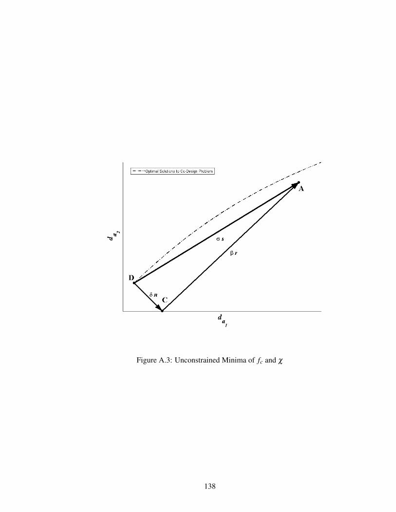
Figure A.3: Unconstrained Minima of fc and χ
138

to point A is denoted as σ , and the distance from point C to point A is denoted as β . The
vectors n, r, and s in Fig. (A.3) are unit vectors.
The function fc evaluated at point A shall be represented by a second-order Taylor
series expansion about its minimum, point D, as follows:
f Ac = f D
c +12
σ2sT
∇2 f D
c s. (A.60)
The function χ evaluated at point A shall be represented by a second-order Taylor series
expansion about its minimum, point C, as follows:
χA = χ
C +12
β2rT
∇2χ
Cr. (A.61)
It is then possible to find the gradients of fc and χ , evaluated at point A, in the da-space.
∇ f Ac = σsT
∇2 f D
c (A.62)
∇χA = βrT
∇2χ
C (A.63)
The unit vector r can be expressed as
r =1β
(σs−δn) (A.64)
and therefore Eq. (A.63) can be re-written as
∇χA = (σs−δn)T
∇2χ
C. (A.65)
From Eq. (A.23), it is known that
cosξA =
∇χA •∇ f Ac
‖∇χA‖‖∇ f Ac ‖
(A.66)
139

which can be re-written as
cosξA =
(σs−δn)T∇2χA∇2 f DT
c s((σs−δn)T
∇2χC∇2χCT (σs−δn))1/2 (
sT ∇2 f Dc ∇2 f DT
c s)1/2
(A.67)
The unit vector s can be expressed in terms of the unit vector n by means of a rotation
matrix, R.
s=Rn (A.68)
which can be substituted into Eq. (A.67). Thus, Eq. (A.67) can be re-written as
cosξA =
nT(
σRT ∇2χC∇2 f DT
c R−δ∇2χC∇2 f DT
c R)n
T1T2(A.69)
where
T1 =(n(
σ2RT
∇2χ
C∇
2χ
CTR−2σδ∇
2χ
C∇
2χ
CTR+δ
2∇
2χ
C∇
2χ
CT)n)1/2
(A.70)
T2 =(nT(RT
∇2 f D
c ∇2 f DT
c R)n)1/2
(A.71)
Note that, since χ (da) achieves its minimum at point C, ∇2χC must be a positive defi-
nite matrix. Likewise, since fc achieves its minimum at point D, ∇2 f Dc must also be positive
definite. The matrixR must also be positive definite.
The monotonicity of cosξ A with respect to δ can now be established. If δ > 1, then an
increase in δ will result in a decrease of the numerator of Eq. (A.69). The denominator of
Eq. (A.69) will increase, and therefore, cosξ A will decrease.
If δ > 1, then an increase in δ will result in an increase in both the numerator and
denominator of Eq. (A.69). However, the denominator will increase at a slower rate than
the numerator due to the relative exponents, and therefore cosξ A will decrease. Since an
increase in δ will always result in a decrease in cosξ A, the function cosξ A is monotonically
decreasing with respect to δ .
140

A decrease in cosξ A will result in an increase in ξ A; thus, we see that an increase in the
distance δ between the minima of fc and χ will result in an increase in the angle ξ A. From
Theorem 4.2, we can then state that an increase in δ will result in CPF solutions that are
farther from the Pareto optimal solutions to the co-design problem, and thus the theorem is
proven.
141

APPENDIX B
Derivation of Artifact and Control Objective and
Constraints for MEMS Actuator
Formulation of Artifact Objective Function
The objective function chosen for the design problem was the negative of the verti-
cal displacement of the actuator, ∆Z. The negative was chosen in order to formulate the
problem as a minimization. From Eq. (4b) in Tung and Kurabayashi’s paper [Tung and
Kurabayashi (2005)], this is given by (see Fig. 5.2)
∆Z = l sinθo− l sin(θo−∆θ) (B.1)
where
l =√
(t + p)2 +(h1 +h2)2 (B.2)
tanθo =h1 +h2
t + p(B.3)
∆θss =A(∆θss)V 2
ssK
(B.4)
142
A(∆θ) =nεohl
d(sinθo− cosθo∆θ) (B.5)
K = KSil2 sin2θo +2KPDMS (B.6)
KSi =2ESihb3
l3Si
(B.7)
KPDMS =EPDMSI
p(B.8)
I =wh3
13
(B.9)
h = h1 +h2 (B.10)
The dimensions t, p, h1, and h2 are shown in Fig. 5.4. The kinematics of the hinge
are modeled as though it were a link of length l, with an angle of θo when not actuated
[Tung and Kurabayashi (2005)]. The change in the angle of the hinge is ∆θ . The variables
K, C, and M represent the effective stiffness, damping, and mass of the entire system,
respectively. The stiffness of the the silicon springs is denoted by KSi and the stiffness of
the PDMS hinge by KPDMS. The constants ESi, EPDMS, and εo are Young’s modulus for
silicon, Young’s modulus for PDMS, and the permittivity of vacuum, respectively. The
dimensions d and w are shown in Fig. 5.5. The variables h, b, and n represent the overall
height of the comb drive, the thickness of the silicon springs, and the number of fingers in
the comb drive, respectively.
In the case of Eq. (B.9), the moment of inertia, I, was taken about the edge rather
than the centroid of the cross-section due to the nature of the hinge. The upper edge is not
restrained in the same way as the lower edge, which should have the result of shifting the
neutral axis from the centroid.
143

Solving Eq. (B.4) and (B.5) for ∆θss yields Eq. (B.14), as shown below.
∆θss =A(∆θss)V 2
ssK
=V 2
ssK
(nεohl
d(sinθo− cosθo∆θss)
)(B.11)
∆θss
(1+
V 2ssnεohl
Kdcosθo
)=
V 2ssnεohl
Kdsinθo (B.12)
∆θss(Kd +V 2
ssnεohl cosθo)
= V 2ssnεohl sinθo (B.13)
∆θss =V 2
ssnεohl sinθo
Kd +V 2ssnεohl cosθo
(B.14)
Substituting Eqs. (B.2), (B.3), and (B.6) - (B.10) into Eq. (B.1) and Eq. (B.14) yields
equations involving only ∆θ , ∆Z, the design variables t, p, h1, and h2, and the constants
and parameters of the problem.
∆θss =V 2
ssnεo (h1 +h2)2
Kd +V 2ssnεo (h1 +h2)(t + p)
(B.15)
∆θss =V 2
ssnεo (h1 +h2)2(
KSil2 sin2θo +2KPDMS
)d +V 2
ssnεo (h1 +h2)(t + p)(B.16)
∆θss =V 2
ssnεo (h1 +h2)2(
KSi (h1 +h2)2 +2KPDMS
)d +V 2
ssnεo (h1 +h2)(t + p)(B.17)
Substituting Eqs. (B.7) - (B.8),
∆θss =V 2
ssnεo (h1 +h2)2((
ESib3
l3Si
)(h1 +h2)
3 +(
EPDMSIp
))2d +V 2
ssnεo (h1 +h2)(t + p)(B.18)
∆θss =V 2
ssnεo (h1 +h2)2((
ESib3
l3Si
)(h1 +h2)
3 + EPDMSwh31
3p
)2d +V 2
ssnεo (h1 +h2)(t + p)(B.19)
144

∆Zss = l sinθo− l sin(θo−∆θss) (B.20)
∆Zss = l (sinθo− sinθo cos∆θss + cosθo sin∆θss) (B.21)
∆Zss = l((
h1 +h2
l
)−(
h1 +h2
l
)cos∆θss +
(t + p
l
)sin∆θss
)(B.22)
∆Zss = (h1 +h2)(1− cos∆θss)+(t + p)sin∆θss (B.23)
The coefficients M, C, and K which appear in the state-space representation of the sys-
tem dynamics in Eq. (5.7) were given in [Tung and Kurabayashi (2005)]. The expressions
for C and K are used in this work, without modification; however, in this problem formu-
lation, an additional term was incorporated in M. The development of M in [Tung and
Kurabayashi (2005)] was based on the assumption that the mass of the hinge was small
compared to the mass of the silicon shuttle and the PDMS platform, but as the design
variables change, this may not always be the case; therefore the mathematical model was
modified to include this effect. The given expression for M was
M = MSil2 sin2θo +MPDMSl2 cos2
θo. (B.24)
The contribution of the hinge is found following a similar procedure to that used in for
the contributions of the platform and shuttle [Tung and Kurabayashi (2005)]. The kinetic
energy of the moving hinge is given by
Thinge =12
Mhingev2cghinge
+12
Ihinge∆θ2. (B.25)
Assuming that the hinge is long and thin, it can be modeled as a rod, and its inertia is given
by
Ihinge =1
12Mhingel2. (B.26)
145

The velocity of the center of gravity of the hinge satisfies the equation
v2cghinge
= v2cgx
+ v2cgy
(B.27)
v2cghinge
=(
∆X− l2
∆θ sin(θo−∆θ))2
+(
l2
∆θ cos(θo−∆θ))2
(B.28)
Since ∆X is given by
∆X = l cos(θo−∆θ)− l cosθo, (B.29)
its time derivative ∆X is found to be
∆X = l sin(θo−∆θ)∆θ (B.30)
and therefore the kinetic energy of the hinge can be expressed as follows:
Thinge =12
Mhinge
((l2
sin(θo−∆θ)∆θ
)2
+(
l2
cos(θo−∆θ)∆θ
)2)
+12
(112
Mhingel2)
∆θ2
(B.31)
Thinge =12
Mhinge∆θ2(
l2
4(sin2 (θo−∆θ)+ cos2 (θo−∆θ)
)+
l2
12
)(B.32)
Thinge =16
Mhingel2∆θ
2 (B.33)
The equation of motion was found by using the Lagrangian, as detailed in Eq. (14) of [Tung
and Kurabayashi (2005)]. The additional term in the system differential equation is given
byddt
(∂Thinge
∂∆θ
)=
ddt
(13
Mhingel2∆θ
)=
13
Mhingel2∆θ (B.34)
146

and therefore, for the mathematical model used in this work,
M = MSil2 sin2θo +MPDMSl2 cos2
θo +13
Mhingel2. (B.35)
The mass terms in Eq. (B.35) are as follows:
MSi = ρSi (h1 +h2)(0.5(wl1 +2l2l3 + l4 (nd +(n−1)3d))+ndl f
)(B.36)
MPDMS =14
ρPDMSl2p (2h1 +h2) (B.37)
Mhinge = ρPDMSw(2h1t + p(2h1 +h2)) (B.38)
The dimensions used in Eq. (B.36) - (B.38) are shown in Fig. 5.4.
Note that, in the derivation of these equations, it is assumed that the device remains
small. If the optimization results were to indicate that the size of the actuator was substan-
tially larger than the original design, then then model developed here would no longer be
valid.
Formulation of Artifact Constraints
The stresses in the actuator are found from the theory of a beam under concentrated
end loading. For purposes of this analysis, it was assumed that the weight of the actuator is
much less than the externally applied forces. The maximum stress in the silicon spring is
given by [Bao (2005)]
σSimax =6MoglSi
hb2 (B.39)
where Mo is the moment in the spring, and g is the acceleration due to gravity. The moment
in the spring, Mo, is related to the deflection, ∆X , by
∆X2
=4Mogl3
SiESihb3 , (B.40)
147

yielding
σSimax =3ESib∆X
4l2Si
. (B.41)
The maximum stress in the PDMS micro-hinge is given by [Bao (2005)],
σPDMSmax =Fth1
2I, (B.42)
where the force F in the hinge, under static conditions, is given by [Tung and Kurabayashi
(2005)]
Ft =EPDMSI∆θss
p. (B.43)
This yields a relation for the maximum steady-state stress in the hinge of
σPDMSmax =EPDMSh1∆θss
2p. (B.44)
148

BIBLIOGRAPHY
149

BIBLIOGRAPHY
Abdalla, M., C. Reddy, W. Faris, and Z. Gurdal (2005), Optimal design of an electrostat-ically actuated microbeam for maximum pull-in voltage, Computers & Structures, 83,1320–1329.
Allison, J., M. Kokkolaras, and P. Papalambros (2005), On the impact of coupling strengthon complex system optimization for single-level formulations, in ASME 2005 Interna-tional Design Engineering Technical Conferences & Computers and Information in En-gineering Conference, ASME, Long Beach, CA, paper number DETC2005-84790.
Alyaqout, S. (2006), A Multi-System Optimization Approach to Coupling in Robust De-sign and Control, PhD Thesis, University of Michigan, Ann Arbor, MI.
Alyaqout, S. F., P. Y. Papalambros, and A. G. Ulsoy (2005), Quantification and use ofsystem coupling in decomposed design optimization problems, in Proceedings of theASME IMECE 2005, pp. 95–103, ASME, Orlando, FL, paper number IMECE2005-81364.
Athan, T. (1994), A quasi-Monte Carlo method for multicriteria optimization, PhD Thesis,University of Michigan, Ann Arbor, MI.
Athan, T., and P. Y. Papalambros (1996), A note on weighted criteria methods for compro-mise solution in multi-objective optimization, Engineering Optimization, 27, 155–176.
Balling, R., and J. Sobieszczanski-Sobieski (1996), Optimization of coupled systems: Acritical overview of approaches, AIAA Journal, 34, 6–17.
Bao, M. (2005), Analysis and Design Principles of MEMS Devices, Elsevier, San Diego,CA.
Belvin, W., and K. Park (1990), Structural tailoring and feedback control synthesis: Aninterdisciplinary approach, Journal of Guidance, Control, and Dynamics, 13, 424–428.
Bloebaum, C. (1995), Coupling strength-based system reduction for complex engineeringdesign, Structural Optimization, 10, 113–121.
Bodden, D., and J. Junkins (1985), Eigenvalue optimization algorithms for struc-ture/controller design iterations, Journal of Guidance, Control, and Dynamics, 8, 697–706.
150

Brown, R. G. (1966), Not just observable, but how observable?, Proceedings of the 1966National Electronic Conference, 22, 709–714.
Brusher, G., P. Kabamba, and A. G. Ulsoy (1997a), Trade-offs between performance spec-ifications, uncertainty and admissible models, in Proceedings of the American ControlConference, pp. 3646–3651, ACC, Albuquerque, NM.
Brusher, G., P. Kabamba, and A. G. Ulsoy (1997b), Coupling between the modeling andcontroller-design problems - part II: Design, Journal of Dynamic Systems, Measurement,and Control, 119, 278–283.
Bryson, A., and Y. Ho (1975), Applied Optimal Control, Hemisphere Publishing Corpora-tion, New York, NY.
Carley, L., G. Ganger, D. Guillou, and D. Nagle (2001), System design considerations forMEMS-actuated magnetic-probe-based mass storage, IEEE Transactions on Magnetics,37, 657–662.
Chen, C., and C. Cheng (2005), Integrated design for a mechatronic feed drive system ofmachine tools, in IEEE/ASME International Conference on Advanced Intelligent Mecha-tronics, Monterey, CA.
Chen, C., and C. Cheng (2006), 3D model-based design for control of a mechatronic ma-chine tools system, Materials Science Forum, 505, 967–972.
Chu, P., et al. (2005), Design and nonlinear servo control of MEMS mirrors and theirperformance in a large port-count optical switch, Journal of MicroelectromechanicalSystems, 14, 261–273.
Das, I. (1999), On characterizing the “knee” of the Pareto curve based on normal-boundaryintersection, Structural and Multidisciplinary Optimization, 18(2), 107–115.
Das, I., and J. Dennis (1997), A closer look at drawbacks of minimizing weighted sumsof objectives for Pareto set generation in multicriteria optimization problems, StructuralOptimization, 14, 63–69.
Eastep, F., N. Khot, and R. Grandhi (1987), Improving the active vibrational control oflarge space structures through structural modifications, Acta Astronautica, 15, 383–389.
Fathy, H. (2003), Combined Plant and Control Optimization: Theory, Strategies and Ap-plications, PhD Thesis, University of Michigan, Ann Arbor, MI.
Fathy, H., S. Bortoff, G. Copeland, P. Y. Papalambros, and A. G. Ulsoy (2002), Nestedoptimization of an elevator and its gain-scheduled LQG controller, in Proceedings of theASME IMECE 2002, pp. 119–126, ASME, New Orleans, LA, iMECE2002-34273.
Fathy, H., D. Hrovat, P. Y. Papalambros, and A. G. Ulsoy (2003), Nested plant/controlleroptimization and its application to combined passive/active automotive suspensions, inProceedings of the American Control Conference, pp. 3375–3380, IEEE, Denver, CO.
151
Fathy, H., P. Y. Papalambros, and A. G. Ulsoy (2004), On combined plant and controloptimization, in 8th Cairo University International Conference on Mechanical Designand Production, Cairo University, Cairo, Egypt.
Franklin, G., J. Powell, and A. Emami-Naeini (1994), Feedback Control of Dynamic Sys-tems, Addison-Wesley Publishing Company, Reading, MA.
Frischknecht, B., D. L. Peters, and P. Y. Papalambros (2009), Pareto set analysis: Localmeasures of objective coupling in multi-objective design optimization, in Proceedingsof the 8th World Congress on Structural and Multidisciplinary Optimization, Lisbon,Portugal.
Grigoriadis, K., and R. Skelton (1998), Integrated structural and control design for vectorsecond-order systems via LMIs, in Proceedings of the American Control Conference, pp.1625–1629, IEEE, Philadelphia, PA.
Haftka, R. (1990), Integrated structure/control optimization of space structures, in Pro-ceedings of the AIAA Dynamics Specialists Conference, pp. 1–9, AIAA, Long Beach,CA.
Haftka, R., Z. Martinovic, W. H. Jr., and G. Schamel (1986), An analytical and experimen-tal study of a control system’s sensitivity to structural modifications, AIAA Journal, 25,310–315.
Hale, A., R. Lisowski, and W. Dahl (1985), Optimal simultaneous structural and controldesign of maneuvering flexible spacecraft, Journal of Guidance, Control, and Dynamics,8, 86–93.
Ionescu, V., C. Oara, and M. Weiss (1999), Generalized Riccati Theory and Robust Control,John Wiley & Sons Ltd., West Sussex, England.
Isermann, R. (1996a), Modeling and design methodology for mechatronic systems,IEEE/ASME Transactions on Mechatronics, 1, 16–28.
Isermann, R. (1996b), On the design and control of mechatronic systems - a survey, IEEETransactions on Industrial Electronics, 43, 4–15.
Junkins, J., and Y. Kim (1993), Introduction to Dynamics and Control of Flexible Struc-tures, American Institute of Aeronautics and Astronautics, Inc., Washington, D.C.
Kailath, T. (1980), Linear Systems, Prentice-Hall, Inc., Englewood Cliffs, NJ.
Kajiwara, I., and R. Haftka (2000), Integrated design of aerodynamics and control systemfor micro air vehicles, JSME International Journal, 43, 684–690.
Khot, N., and N. Abhyankar (1993), Integrated optimum structural and control design, inStructural Optimization: Status and Promise, edited by M. P. Kamat, Washington, D.C.
152

Kitayama, S., K. Yamazaki, M. Arakawa, and H. Yamakawa (2009), Quantitative trade-offanalysis and its application to the compromise solution in the multi-objective design op-timization, in Proceedings of the 8th World Congress on Structural and MultidisciplinaryOptimization, WCSMO, Lisbon, Portugal.
Kosut, R., G. Kabuli, S. Morrison, and Y. Harn (1990), Simultaneous control and structuredesign for large space structures, in Proceedings of the American Control Conference,pp. 860–865, IEEE, San Diego, CA.
Kuhn, H. W., and A. W. Tucker (1950), Nonlinear programming, in Proceedings of theSecond Berkeley Symposium on Mathematical Statistics and Probability, pp. 481–492,University of California, Berkeley, CA.
Legtenberg, R., A. Groeneveld, and M. Elwenspoek (1996), Comb-drive actuators for largedisplacements, Journal of Micromechanical Microengineering, 6, 320–329.
Li, Q., W. Zhang, and L. Guo (1999), Integrated design and control for a programmablefour-bar linkage, in Proceedings of the ASME Design Engineering Technical Conference,ASME, Las Vegas, NV, paper number DAC99/DAC8663.
Li, Q., W. Zhang, and L. Chen (2001), Design for control - a concurrent engineering ap-proach for mechatronic systems design, IEEE/ASME Transactions on Mechatronics, 6,161–169.
Lim, K., and W. Gawronski (1993), Modal Grammian approach to actuator and sensorplacement for flexible structures, AIAA Journal, 31, 674–684.
Maghami, P., S. Gupta, K. Elliott, and S. Joshi (1996), Experimental validation of an inte-grated controls-structures design methodology, Journal of Guidance, Control, and Dy-namics, 19, 324–333.
Messac, A. (1998), Control-structure integrated design with closed-form design metricsusing physical programming, AIAA Journal, 36, 855–864.
Messac, A., and C. Puemi-Sukam (2000), Aggregate objective functions and Pareto fron-tiers: Required relationships and practical implications, Optimization and Engineering,1, 171–188.
Milman, M., M. Salama, R. Scheid, R. Bruno, and J. Gibson (1991), Combined control-structural optimization, Computational Mechanics, 8, 1–18.
Muller, P. C., and H. I. Weber (1972), Analysis and optimization of certain qualities ofcontrollability and observability for linear dynamical systems, Automatica, 8, 237–246.
Oldham, K., X. Huang, A. Chahwan, and R. Horowitz (2005), Design, fabrication andcontrol of a high-aspect ratio microactuator for vibration suppression in a hard disk drive,in Proceedings of the IFAC World Congress, Prague.
153

Onoda, J., and N. Watanabe (1989), Integrated direct optimization of struc-ture/regulator/observer for large flexible spacecraft, AIAA Journal, 27, 1336–1344.
Ou, J., and N. Kikuchi (1996), Integrated optimal structural and vibration control design,Structural Optimization, 12, 209–216.
Ouyang, P., W. Zhang, and F. Wu (2002), Nonlinear PD control for trajectory tracking withconsideration of the design for control methodology, in Proceedings of the IEEE In-ternational Conference on Robotics & Automation, pp. 4126–4131, IEEE, Washington,D.C.
Papalambros, P., and D. Wilde (2000), Principles of Optimal Design: Modeling and Com-putation, Cambridge University Press, Cambridge, NY.
Park, J., and H. Asada (1992), Integrated structure/control design of a two-link nonrigidrobot arm for high speed positioning, in Proceedings of the IEEE International Confer-ence on Robotics & Automation, IEEE, Nice, France.
Park, S., and R. Horowitz (2003), Adaptive control for the conventional mode of operationof MEMS gyroscopes, Journal of Microelectromechanical Systems, 12, 101–108.
Peters, D. L., K. Kurabayashi, P. Y. Papalambros, and A. G. Ulsoy (2008), Co-designof a MEMS actuator and its controller using frequency constraints, in Proceedings ofthe ASME Dynamic Systems and Control Conferences, ASME, Ann Arbor, MI, papernumber DSCC 2008-2212.
Peters, D. L., P. Y. Papalambros, and A. G. Ulsoy (2009), On measures of coupling betweenthe artifact and controller optimal design problems, in Proceedings of the ASME DesignEngineering Technical Conference & Computers in Engineering Conference, ASME,San Diego, CA, paper number DETC 2009-86868.
Peters, D. L., P. Y. Papalambros, and A. G. Ulsoy (2010), Relationship between couplingand the controllability Grammian in co-design problems, in Proceedings of the AmericanControl Conference, ASME, Baltimore, MD, (submitted).
Pil, A., and H. Asada (1996), Integrated structure/control design of mechatronic sys-tems using a recursive experimental optimization method, IEEE/ASME Transactions onMechatronics, 1, 191–203.
Pomrehn, L., and P. Papalambros (1994), Global and discrete constraint activity, Journalof Mechanical Design, 116, 745–748.
Rao, S., and T. Pan (1990), Modeling, control, and design of flexible structures: A survey,Applied Mechanics Review, 43, 99–117.
Ravichandran, T., D. Wang, and G. Heppler (2006), Simultaneous plant-controller designoptimization of a two-link planar manipulator, Mechatronics, 16, 233–242.
154

Reyer, J. (2000), Combined Embodiment Design and Control Optimization: Effects ofCross-Disciplinary Coupling, PhD Thesis, University of Michigan, Ann Arbor, MI.
Roh, H., and Y. Park (1997), Actuator and exciter placement for flexible structures, Journalof Guidance, Control, and Dynamics, 20, 850–856.
Shabde, V. S., and K. A. Hoo (2008), Optimum controller design for a spray drying process,Control Engineering Practice, 16(5), 541–552.
Skogestad, S., and I. Postlethwaite (2005), Multivariable Feedback Control: Analysis andDesign, John Wiley and Sons, Ltd., West Sussex, UK.
Sobieszczanski-Sobieski, J., and R. Haftka (1997), Multidisciplinary aerospace design op-timization: Survey of recent developments, Structural Optimization, 14, 1–23.
Steuer, R. E. (1986), Multiple Criteria Optimization: Theory, Computation, and Applica-tion, John Wiley and Sons, Inc., New York, NY.
Tilbury, D., and S. Kota (1999), Integrated machine and control design for reconfigurablemachine tools, in Proceedings of the IEEE/ASME International Conference on AdvancedIntelligent Mechatronics, IEEE/ASME, Atlanta, GA.
Tung, Y., and K. Kurabayashi (2005), A single-layer PDMS-on-silicon hybrid microactua-tor with multi-axis out-of-plane motion capabilities - part I: Design and analysis, Journalof Microelectromechanical Systems, 14, 548–557.
Wan, J., Q. Li, and F. Wu (2002), Integrated design and control of a closed-chain mecha-nism, in Proceedings of the Seventh International Conference on Control, Automation,Robotics and Vision, pp. 1349–1353, IEEE, Singapore.
Wolfram, H., R. Schmiedel, K. Hiller, T. Aurich, W. Gunther, S. Kurth, J. Mehner,W. Dotzel, and T. Gebner (2005), Model building, control design and practical imple-mentation of a high precision, high dynamical MEMS acceleration sensor, in Society ofPhoto-Optical Instrumentation Engineers, pp. 1–15, SPIE, Sevilla, Spain.
Yee, E., and Y. Tsuei (1991), Method for shifting natural frequencies of damped mechanicalsystems, AIAA Journal, 29, 1973–1977.
Youcef-Toumi, K. (1996), Modeling, design, and control integration: A necessary step inmechatronics, IEEE/ASME Transactions on Mechatronics, 1, 29–38.
Zhang, J., M. Wiecek, and W. Chen (1999), Local approximation of the efficient frontier inrobust design, in Proceedings of the ASME Design Engineering Technical Conferences,ASME, Las Vegas, NV, paper number DETC99/DAC-8566.
Zhu, Y., J. Qiu, and J. Tani (2001), Simultaneous optimization of a two-link flexible robotarm, Journal of Robotic Systems, 18, 29–38.
155