coupling of the meshfree and ﬁnite element methods for determination of ... · coupling of the...

Available online at www.sciencedirect.com

Engineering Fracture Mechanics 75 (2008) 986–1004

www.elsevier.com/locate/engfracmech

Coupling of the meshfree and finite element methodsfor determination of the crack tip fields

Y.T. Gu a,b, L.C. Zhang b,*

a School of Engineering Systems, Queensland University of Technology, G.P.O. Box 2434, Brisbane, QLD 4001, Australiab School of Aerospace, Mechanical and Mechatronic Engineering, The University of Sydney, NSW 2006, Australia

Received 28 November 2006; received in revised form 3 May 2007; accepted 3 May 2007Available online 16 May 2007

Abstract

This paper develops a new concurrent simulation technique to couple the meshfree method with the finite elementmethod (FEM) for the analysis of crack tip fields. In the sub-domain around a crack tip, we applied a weak-form basedmeshfree method using the moving least squares approximation augmented with the enriched basis functions, but in theother sub-domains far away from the crack tip, we employed the finite element method. The transition from the meshfreeto the finite element (FE) domains was realized by a transition (or bridge region) that can be discretized by transition par-ticles, which are independent of both the meshfree nodes and the FE nodes. A Lagrange multiplier method was used toensure the compatibility of displacements and their gradients in the transition region. Numerical examples showed thatthe present method is very accurate and stable, and has a promising potential for the analyses of more complicated crack-ing problems, as this numerical technique can take advantages of both the meshfree method and FEM but at the same timecan overcome their shortcomings.� 2007 Elsevier Ltd. All rights reserved.

Keywords: Crack; Meshfree; Meshless; Finite element method; Concurrent simulation; Fracture mechanics; Numerical analysis

1. Introduction

The finite element method (FEM) is currently a dominant numerical tool in the analysis of fracturemechanics problems, especially for stationary cracks. A large variety of approaches have been developed inthe analysis of the field of crack tip by FEM. However, FEM often experiences difficulties in re-meshingand adaptive analysis. In addition, FEM is often difficult (or even impossible) to simulate some problems suchas the large deformation problems with severe element distortions, crack growth problems with arbitrary andcomplex paths which do not coincide with the original element interfaces, and the problems of breakage ofmaterial with large number of fragments. Meshfree (or meshless) methods have recently become attractivealternatives for problems in computational mechanics, as they do not require a mesh to discretize the problem

0013-7944/$ - see front matter � 2007 Elsevier Ltd. All rights reserved.

doi:10.1016/j.engfracmech.2007.05.003

* Corresponding author. Fax: +61 2 93517060.E-mail address: [email protected] (L.C. Zhang).

mailto:[email protected]

Nomenclature

a vector of interpolation coefficients, defined in Eq. (2)A, B interpolation matrices, defined in Eqs. (7) and (8)A(FE), A(MM) transition matrices for FEM and meshfree method, defined in Eqs. (44) and (45)b vector of body force, defined in Eq. (14)B(FE), B(MM) transition matrices for FEM and meshfree method, defined in Eqs. (36) and (38)D Matrix of material constantsf(MM)k, f(MM)k force vectors at a particle k obtained by the FEM and meshfree method, defined in Eqs.

(26) and (27)F(FE), F(MM) force vectors for FEM and meshfree method, defined in Eqs. (23) and (24)g generalized displacement of a transition particle, defined in Eq. (28)g(x) generalized derivative of a transition particle, defined in Eq. (41)KI, KII, KIII stress intensity factors for mode-I, mode-II, and mode-IIIK(FE), K(MM) stiffness matrices for FEM and meshfree method, defined in Eqs. (21) and (22)n vector of the unit outward normal, defined in Eq. (14)N FEM shape function, defined in Eq. (18)pj monomial of polynomial basis functions, defined in Eq. (2)(R, h) cylindrical coordinate, defined in (10)u displacement vector, defined in Eq. (14)u(MM)k, u(MM)k displacement vectors at a particle k obtained by the FEM and meshfree method, defined

in Eqs. (26) and (27)�u; �t prescribed boundary displacement and traction, defined in Eqs. (15) and (16)w weight function, defined in Eq. (3)x coordinate vectorC global boundary/ shape function, defined in Eq. (6)U shape function matrix, defined in Eq. (29)P functionalCu, Ct boundaries for displacement and traction boundary conditions, defined in Eqs. (15) and (16)e, r vectors of strain and stress, defined in Eqs. (17) and (14)k, c Lagrange multiplier, defined in Eqs. (34) and (42)K, W selected interpolation for k and c, defined in Eqs. (34) and (44)X problem domainXs local domain to construct meshfree shape functions

Y.T. Gu, L.C. Zhang / Engineering Fracture Mechanics 75 (2008) 986–1004 987

domain, and the approximate solution is constructed entirely by a set of scattered nodes. Some meshfree meth-ods have been developed and achieved remarkable progress, such as the smooth particle hydrodynamics(SPH) [1], the element-free Galerkin (EFG) method [2], the reproducing kernel particle method (RKPM)[3,4], the meshfree local Petrov–Galerkin (MLPG) method [5–7], and the local radial point interpolationmethod (LRPIM) [8–11]. The principal attraction of the meshfree methods is their capacity in dealing withmoving boundaries and discontinuities, such as phase changes and crack propagations, and their ease in usingthe enriched basis functions based on the asymptotic displacement fields near the crack tip [12].

However, the meshfree method usually has worse computational efficiency than FEM, because more com-putational cost is required in the meshfree interpolation and numerical integrations [13]. Although the burdenof the computational cost is being alleviated due to the development of computer technologies, to improve thecomputational efficiency is still a key factor for the simulations of many practical problems, for example, thethree-dimensional dynamic crack problem, etc. Some strategies have been developed for the alleviation of theabove-mentioned problems, but how to improve the efficiency of the meshfree methods is still an open prob-lem. Coupling the meshfree methods with FEM can be a possible solution.

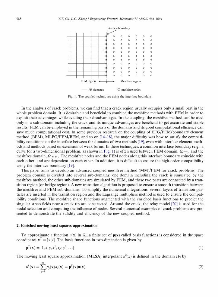
FE elements meshfree nodes

Interface boundary

I

Meshfree region FEM region

Fig. 1. The coupled techniques using the interface boundary.

988 Y.T. Gu, L.C. Zhang / Engineering Fracture Mechanics 75 (2008) 986–1004

In the analysis of crack problems, we can find that a crack region usually occupies only a small part in thewhole problem domain. It is desirable and beneficial to combine the meshfree methods with FEM in order toexploit their advantages while evading their disadvantages. In the coupling, the meshfree method can be usedonly in a sub-domain including the crack and its unique advantages are beneficial to get accurate and stableresults. FEM can be employed in the remaining parts of the domains and its good computational efficiency cansave much computational cost. In some previous research on the coupling of EFG/FEM/boundary elementmethod (BEM), MLPG/FEM/BEM, and so on [14–18], the major difficulty was how to satisfy the compati-bility conditions on the interface between the domains of two methods [19], even with interface element meth-ods and methods based on extension of weak forms. In these techniques, a common interface boundary (e.g., acurve for a two-dimensional problem, as shown in Fig. 1) is often used between FEM domain, X(FE), and themeshfree domain, X(MM). The meshfree nodes and the FEM nodes along this interface boundary coincide witheach other, and are dependent on each other. In addition, it is difficult to ensure the high-order compatibilityusing the interface boundary [19].

This paper aims to develop an advanced coupled meshfree method (MM)/FEM for crack problems. Theproblem domain is divided into several sub-domains: one domain including the crack is simulated by themeshfree method, the other sub-domains are simulated by FEM, and these two parts are connected by a tran-sition region (or bridge region). A new transition algorithm is proposed to ensure a smooth transition betweenthe meshfree and FEM sub-domains. To simplify the numerical integrations, several layers of transition par-ticles are inserted in the transition region and the Lagrange multipliers method is used to ensure the compat-ibility conditions. The meshfree shape functions augmented with the enriched basis functions to predict thesingular stress fields near a crack tip are constructed. Around the crack, the relay model [20] is used for thenodal selection and computing the influence of nodes. Several numerical examples of crack problems are pre-sented to demonstrate the validity and efficiency of the new coupled method.

2. Enriched moving least squares approximation

To approximate a function u(x) in Xs, a finite set of p(x) called basis functions is considered in the spacecoordinates xT = [x,y]. The basis functions in two-dimension is given by

pTðxÞ ¼ ½1; x; y; x2; xy; y2; . . .� ð1Þ

The moving least square approximation (MLSA) interpolant uh(x) is defined in the domain XS by

uhðxÞ ¼Xm

j¼1

pjðxÞajðxÞ ¼ pTðxÞaðxÞ ð2Þ


where m is the number of basis functions, and the coefficients aj(x) are also functions of x; a(x) is obtained atany point x by minimizing a weighted discrete L2 norm of:

J ¼Xn

i¼1

wðx� xiÞ½pTðxiÞaðxÞ � ui�2 ð3Þ

where n is the number of nodes in the neighborhood of x for which the weight function w(x � xi) 5 0, and ui isthe nodal value of u at x = xi.

The stationarity of J with respect to a(x) leads to the following linear relation between a(x) and u:

AðxÞaðxÞ ¼ BðxÞu ð4Þ
Solving a(x) from Eq. (4) and substituting it into Eq. (2), we have
uhðxÞ ¼Xn

i¼1

/iðxÞu ð5Þ

where the MLSA shape function /i(x) is defined by

/iðxÞ ¼Xm

j¼1

pjðxÞðA�1ðxÞBðxÞÞji ð6Þ

In which A(x) and B(x) are the matrices defined by

AðxÞ ¼Xn

i¼1

wiðxÞpTðxiÞ; pðxiÞ; where wiðxÞ ¼ wðx� xiÞ ð7Þ

BðxÞ ¼ w1ðxÞpðx1Þ;w2ðxÞpðx2Þ; . . . ;wnðxÞpðxnÞ½ � ð8Þ

It should be mentioned here that the MLSA shape function obtained above does not have the Kroneckerdelta function properties [13].

In two-dimensional linear elastic fracture mechanics, both mode-I and mode-II crack-tip fields should beconsidered. For mode-I deformations, the crack-tip stresses have the following formulations [21]

r11

r22

r12

8><>:

9>=>; ¼

KIffiffiffiffiffiffiffi2prp cos

h2

1� sin h2

sin 3h2

1þ sin h2

sin 3h2

sin h2

sin 3h2

8><>:

9>=>; ð9Þ

For mode-II deformations, the crack-tip stresses are [21]

r11

r22

r12

8><>:

9>=>; ¼

KIIffiffiffiffiffiffiffi2prp cos

h2

� sin h2

2þ cos h2

cos 3h2

� �sin h

2cos h

2cos 3h

2

cos h2

1� sin h2

sin 3h2

� �8><>:

9>=>; ð10Þ

where KI and KII are the stress intensity factors for mode-I and mode-II dependent upon the crack length, thespecimen geometry and the applied loading, and (r,h) are the cylindrical coordinates of a point with the originlocated at the crack tip and the positive angle measured counterclockwise from the axis of the crack.

After using trigonometric identities, one can show that all of the functions in Eqs. (9) and (10) are spannedby the following four basis functions:

ffiffirp

cosh2

ffiffirp

sinh2

ffiffirp

sinh2

sin hffiffirp

cosh2

sin h

� �ð11Þ

In the application of the meshfree method to linear elastic fracture mechanics (LEFM) problems, it isadvantageous to add these four basis functions in Eq. (11) into the basis functions so that the stress singu-larity can be captured without having a very fine nodal density around the crack tip. It was first used byFleming et al. [12] in the element-free Galerkin (EFG) method and called the resulting basis as enrichedbasis functions.


Adding these four basis functions in Eq. (11) into Eq. (1), we can obtain the enriched basis functions for atwo-dimensional problem:

(a) with complete linear monomials

pTðxÞ ¼ 1; x; y;ffiffirp

cosh2;ffiffirp

sinh2;ffiffirp

sinh2

sin h;ffiffirp

cosh2

sin h

� �ð12Þ

(b) with complete second-order monomials

pTðxÞ ¼ 1; x; y; x2; xy; y2;ffiffirp

cosh2;ffiffirp

sinh2;ffiffirp

sinh2

sin h;ffiffirp

cosh2

sin h

� �ð13Þ

3. Discrete equations of FEM and the meshfree method

Consider the following two-dimensional problem of solid mechanics in domain X bounded by C:

rrþ b ¼ 0 in X ð14Þ

where r is the stress tensor, which corresponds to the displacement field u = {u, v}T, b is the body force vector,and $ is the divergence operator. The boundary conditions are given as follows:

u ¼ �u on Cu ð15Þr � n ¼ �t on Ct ð16Þ

in which the superposed bar denotes prescribed boundary values and n is the unit outward normal to domainX.

The principle of minimum potential energy can be stated as follows: The solution of a problem in the smalldisplacement theory of elasticity is the vector function u of displacement which minimizes the total potentialenergy P given by

P ¼Z

X

1

2eT � rdX�

ZX

uT � bdX�Z

Ct

uT ��tdC ð17Þ

with the boundary condition described in Eq. (15), where e is the strain.The meshfree method and FEM use the similar global weak form given in Eq. (17). The meshfree shape

functions have been given in Section 2, and the interpolation formulation of FEM can be written as [22]

u ¼Xne

i¼1

N iðxÞui ne ¼ 3; 4; 5; . . . ð18Þ

where ne is the number of nodes in a FE element, and N is the FE shape function.Substituting the expression of u given in Eqs. (5) and (18), and using the stationary condition for Eq. (17)

yield

KðFEÞUðFEÞ ¼ FðFEÞ ð19ÞKðMMÞUðMMÞ ¼ FðMMÞ ð20Þ

where K(FE), U(FE), F(FE), K(MM), U(MM), and F(MM) are stiffness matrices, the displacement vectors, and theforce vectors for FEM and the meshfree method, respectively. Now, we have


KðFEÞij ¼Z

XBTðFEÞiDBðFEÞjdX ð21Þ

KðMMÞij ¼Z

XBTðMMÞiDBðMMÞjdX ð22Þ

FðFEÞi ¼Z

Ct

NitdCþZ

XNibdX ð23Þ

FðMMÞi ¼Z

Ct

/itdCþZ

X/ibdX ð24Þ

where D is the matrix of material constants, and

BðFEÞi ¼N i;x 0

0 Ni;y

N i;y N i;x

264

375; BðMMÞi ¼

/i;x 0

0 /i;y

/i;y /i;x

264

375 ð25Þ

4. Coupling of the meshfree method and FEM

4.1. Transition condition

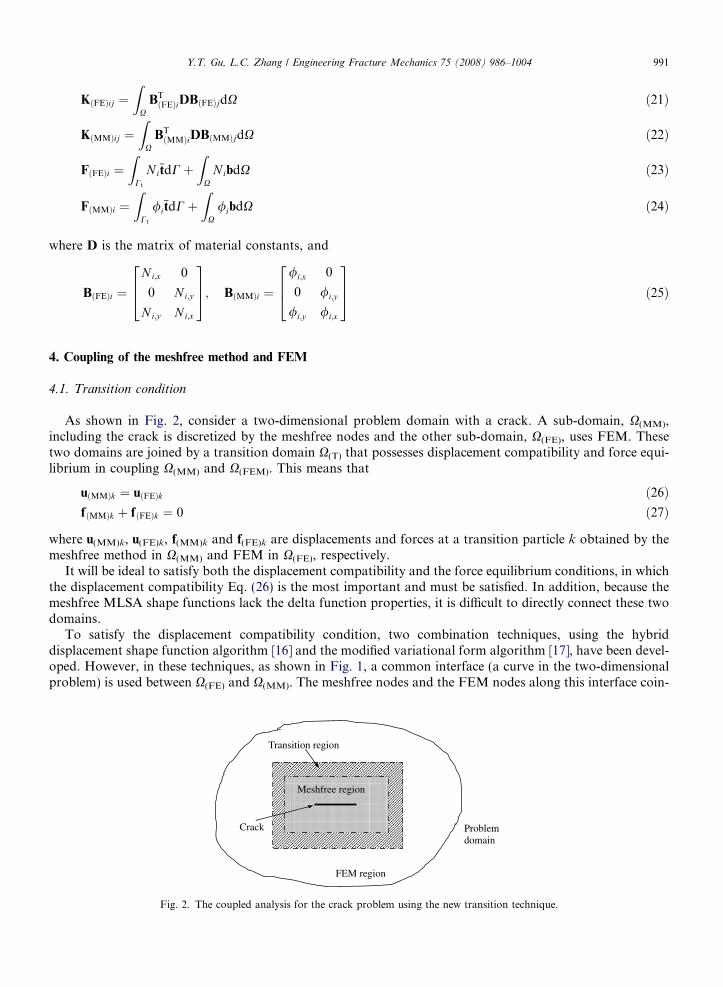
As shown in Fig. 2, consider a two-dimensional problem domain with a crack. A sub-domain, X(MM),including the crack is discretized by the meshfree nodes and the other sub-domain, X(FE), uses FEM. Thesetwo domains are joined by a transition domain X(T) that possesses displacement compatibility and force equi-librium in coupling X(MM) and X(FEM). This means that

uðMMÞk ¼ uðFEÞk ð26ÞfðMMÞk þ fðFEÞk ¼ 0 ð27Þ

where u(MM)k, u(FE)k, f(MM)k and f(FE)k are displacements and forces at a transition particle k obtained by themeshfree method in X(MM) and FEM in X(FE), respectively.

It will be ideal to satisfy both the displacement compatibility and the force equilibrium conditions, in whichthe displacement compatibility Eq. (26) is the most important and must be satisfied. In addition, because themeshfree MLSA shape functions lack the delta function properties, it is difficult to directly connect these twodomains.

To satisfy the displacement compatibility condition, two combination techniques, using the hybriddisplacement shape function algorithm [16] and the modified variational form algorithm [17], have been devel-oped. However, in these techniques, as shown in Fig. 1, a common interface (a curve in the two-dimensionalproblem) is used between X(FE) and X(MM). The meshfree nodes and the FEM nodes along this interface coin-

FEM region

Meshfree region

Transition region

Crack Problem domain

Fig. 2. The coupled analysis for the crack problem using the new transition technique.


cide with each other, and are dependent on each other. It will increase the computational cost and make dif-ficulty for some problems. In addition, because only an interface curve is used, it is difficult to ensure the com-patibility (especially the high-order continuity). In the following, we will develop a new transition technique toensure a smooth transition between X(FE) and X(MM), which has been successfully used in the macro/micro/nano multiscale analysis [23].

4.2. Coupling technique

As shown in Fig. 2, there is a transition (or bridge) region, X(T), between the FEM and meshfree domains.The generalized displacement of a point in the transition domain at x can be defined as

g ¼ uðMMÞðxÞ � uðFEÞðxÞ ð28Þ

where u(MM)(x) and u(FE)(x) are the displacements of a point x, obtained by the interpolations using the mesh-free nodes and the FEM element, respectively, i.e.,

uðMMÞðxÞ ¼X

I

UIðxÞuðMMÞI ð29Þ

uðFEÞðxÞ ¼X

J

NJ ðxÞuðFEÞJ ð30Þ

A sub-functional is introduced to enforce the displacement compatibility condition given in Eq. (26) bymeans of Lagrange multiplier k in the transition domain

PðTÞ ¼Z

XðTÞ

k � gdX ¼Z

XðTÞ

k � uðMMÞ � uðFEÞ

dX

¼Z

XðTÞ

k � uðMMÞdX�Z

XðTÞ

k � uðFEÞdX

¼ PðMMÞðTÞ �PðFEÞ

ðTÞ

ð31Þ

In which, PðMMÞðTÞ and PðFEÞ

ðTÞ are the sub-functional for the meshfree part and the FEM part. Substituting PðMMÞðTÞ

and PðFEÞðTÞ separately into Eq. (17) for the meshfree method and FEM, their generalized functional forms can

be written as

PðMMÞ ¼Z

XðMMÞ

1

2eT � rdX�

ZXðMMÞ

uT � bdX�Z

CðMMÞt

uT � tdCþZ

XðTÞ

k � uðMMÞdX ð32Þ

PðFEÞ ¼Z

XðFEÞ

1

2eT � rdX�

ZXðFEÞ

uT � bdX�Z

CðFEÞt

uT � tdC�Z

XðTÞ

k � uðFEÞdX ð33Þ

In these variational formulations, the domains of X(FE) and X(MM) are connected via Lagrange multiplier k,which can be given by the interpolation functions K and the nodal value of ki

k ¼X

i

Ki � ki ð34Þ

K is the selected interpolation for ki and it can be the FEM shape function.Substituting Eqs. (5) and (34) into Eq. (32), and using the stationary condition based on the displacement,

the following meshfree equations can be obtained

KðMMÞ BðMMÞ UðMMÞ

k

� �¼ FðMMÞ� �

ð35Þ

where K(MM) and F(MM) have been defined in Eqs. (22) and (24), B(MM) is defined as

BðMMÞ ¼Z

XðTÞ

KUTdX ð36Þ


Substituting Eqs. (18) and (34) into Eq. (33), and using the stationary condition based on the displacement,lead to the following FEM equations

KðFEÞ � BðFEÞ UðFEÞ

k

� �¼ FðFEÞ� �

ð37Þ

where K(FE) and F(FE) have been defined in Eqs. (21) and (23), B(FE) is defined as

BðFEÞ ¼Z

XðTÞ

KN TdX ð38Þ

It should be mentioned here that it is impossible to solve Eqs. (35) and (37) separately. To obtain the uniquesolution for the global problem, using the stationary condition of Eqs. (35) and (37) based on the Lagrangemultiplier and considering the compatibility condition, we can obtain the following relationship,

BTðMMÞUðMMÞ � BT

ðFEÞUðFEÞ ¼ 0 ð39Þ

Because the meshfree and FEM domains are connected through the transition domain, the assembly of Eqs.(35), (37) and (39) yields a linear system of the following form

KðMMÞ 0 BðMMÞ

0 KðFEÞ �BðFEÞ

BTðMMÞ �BT

ðFEÞ 0

264

375

UðMMÞ

UðFEÞ

k

8><>:

9>=>; ¼

FðMMÞ

FðFEÞ

0

8><>:

9>=>; ð40Þ

Solving Eq. (40) together with the displacement boundary condition, given in Eq. (15), we can obtain the solu-tion for the problem considered.

To satisfy the force equilibrium condition, the generalized derivative at a point x can be written as

gðxÞ ¼ouðMMÞðxÞ

ox� ouðFEÞðxÞ

oxð41Þ

Using Lagrange multiplier c, we have

PðTÞðxÞ ¼Z

XðTÞ

c � gdX

¼Z

XðTÞ

c � ouðMMÞðxÞox

dX�Z

XðTÞ

c � ouðFEÞðxÞox

dX

¼ PðMMÞðTÞðxÞ �PðFEÞ

ðTÞðxÞ

ð42Þ

Following the similar procedure from Eqs. (32)–(40), we can obtain the coupling equations to satisfy the high-order continuity

KðMMÞ 0 BðMMÞ AðMMÞ

0 KðFEÞ �BðFEÞ �AðFEÞ

BTðMMÞ �BT

ðFEÞ 0 0

ATðMMÞ �AT

ðFEÞ 0 0

266664

377775

UðMMÞ

UðFEÞ

k

c

8>>><>>>:

9>>>=>>>;¼

FðMMÞ

FðFEÞ

0

0

8>>><>>>:

9>>>=>>>;

ð43Þ

where

AðMMÞ ¼Z

XðTÞ

WoUT

oxdX ð44Þ

AðFEÞ ¼Z

XðTÞ

WoNT

oxdX ð45Þ

In which W are the interpolation functions for c.


4.3. Numerical implementations

(a) The size of transition region. The size of transition region will affect the performance of the coupledmethod. If the size is too small, it will decrease the accuracy of the transition, especially for the high-ordercompatibility. If the size is too big, it will significantly increase the computational cost. For many problems,it is reasonable to use the following size of transition region:

ht ffi ð3 � 5Þ � dFE or ð3 � 5Þ � dMM ð46Þwhere dFE and dMM are equivalent sizes of FEM element and meshfree nodal space.(b) The transition particles. To get B(MM) and B(FEM) numerically, the transition region can be divided intoregular background cells, which are similar to those used in the meshfree method. However, these cells aretotally independent of the FE elements and the meshfree background cells. In the practical computation, tosimplify the integration and reduce the ‘‘meshing’’ cost, several layers of transition particles, which are reg-ularly distributed, can be inserted in the transition domain X(T). The displacement compatibility betweenFEM and meshfree nodes is achieved through these transition particles. The advantages of using these tran-sition particles are clear. First, they allow the meshfree nodes in X(MM) to have an arbitrary distribution andbecome independent of the distributions of the FEM nodes in X(FE). Second, the compatibility conditionsin the transition domain can be conveniently controlled through the adjustment of the number and distri-bution of the transition particles. For some sub-transition domains with stronger compatibility require-ment, a finer transition particle distribution can be arranged. Third, the compatibility of higher orderderivatives can be easily satisfied.(c) Lagrange multipliers. The above Lagrange multiplier method is accurate and the physical meaning isalso very clear. However, it will increase the computational cost (especially when the number of transitionparticles is large) because new variables (Lagrange multipliers) are added. Hence, we can use the constantLagrange multipliers to yield the so-called penalty method, i.e., the common Lagrange multiplier methodcan be used to obtain a range of penalty coefficients, and then use them as constants for this problem andother similar problems to improve computational efficiency.

5. The relay model

With the use of node based interpolation techniques, meshfree methods offer great opportunities to han-dle problems of complex geometry including cracks. However, there is general discontinuity of displace-ments across a crack, and the interpolation domain used for the construction of meshfree shapefunctions can contain numerous irregular boundary fragments and the computation of nodal weights basedon physical distance can be erroneous. This issue will become more serious in dealing with the fractureproblems, especially for the multi-cracking problems. Several techniques have been reported on the con-struction of meshfree approximations with discontinuities and non-convex boundaries, including the visibil-ity method [2], the diffraction method [24], and the transparency method [24]. However, these methods areonly effective for problems with relatively simple domains (e.g., with one or two cracks, or not many non-convex portions on the boundaries), but not effective for domains with highly irregular boundaries (e.g.,with many cracks). Liu and Tu [25] have developed a relay model to determine the domain of influenceof a node in a complex problem domain.

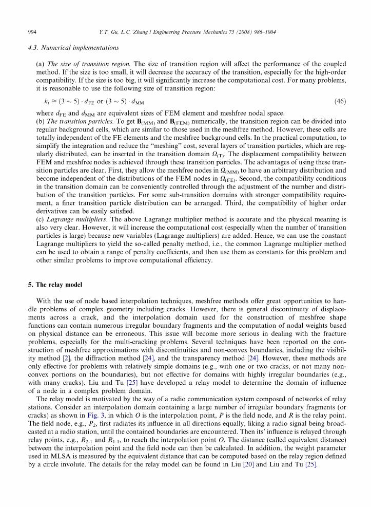
The relay model is motivated by the way of a radio communication system composed of networks of relaystations. Consider an interpolation domain containing a large number of irregular boundary fragments (orcracks) as shown in Fig. 3, in which O is the interpolation point, P is the field node, and R is the relay point.The field node, e.g., P2, first radiates its influence in all directions equally, liking a radio signal being broad-casted at a radio station, until the contained boundaries are encountered. Then its’ influence is relayed throughrelay points, e.g., R2-1 and R1-1, to reach the interpolation point O. The distance (called equivalent distance)between the interpolation point and the field node can then be calculated. In addition, the weight parameterused in MLSA is measured by the equivalent distance that can be computed based on the relay region definedby a circle involute. The details for the relay model can be found in Liu [20] and Liu and Tu [25].

O

crack

**R1-2

R1-1P1

P2

*R2-1

cracks

Interpolation domain

: interpolation node; *: relay points; : field nodes; : reply paths

Fig. 3. Relay model for an irregular domain with discontinuous boundaries.


6. Numerical results and discussions

Several cases of two-dimensional fracture problems have been studied in order to examine the present cou-pled MM/FE method. Except when mentioned, the units are taken as standard international (SI) units in thefollowing examples.

6.1. Cantilever beam

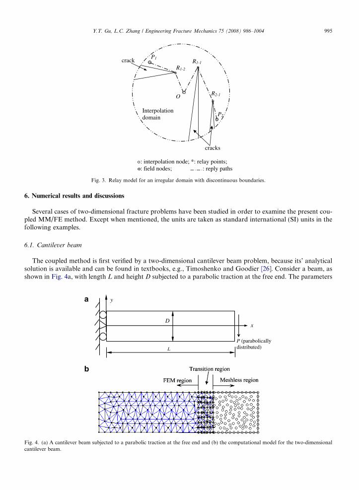
The coupled method is first verified by a two-dimensional cantilever beam problem, because its’ analyticalsolution is available and can be found in textbooks, e.g., Timoshenko and Goodier [26]. Consider a beam, asshown in Fig. 4a, with length L and height D subjected to a parabolic traction at the free end. The parameters

y

P (parabolically distributed)

x

L

D

a

b

Fig. 4. (a) A cantilever beam subjected to a parabolic traction at the free end and (b) the computational model for the two-dimensionalcantilever beam.


of the beam are taken as E = 3.0 · 107, m = 0.3, D = 12, L = 48, and P = 1000. The beam has a unit thicknessand a plane stress problem is considered.

As shown in Fig. 4b, the beam is divided into two parts. FEM using the triangular elements is used in theleft part where the essential boundary condition is included. The meshfree method is used in the right partwhere the traction boundary condition is included. These two parts are connected through a transition regionthat is discretized by 54 regularly distributed transition particles. Fig. 5 illustrates the comparison between theshear stress calculated analytically and by the coupled method at the cross-section of x = L/2, which shows anexcellent agreement between the analytical and numerical results.

6.2. Near-tip crack field

A well-known near-tip field, which is subjected to a mode-I displacement field at its edges, is analyzed. Asshown in Fig. 6, an edge-cracked square plate is subjected to the following displacement field for a model-Icrack [1].

Fig. 5. Shear stress distributions on the cross-section of the beam at x = L/2.

5

10

u

u

u

u

x

y

Fig. 6. A cracked square plate subjected to mode-I displacement boundary conditions.


u

v

� �¼ KI

2l

ffiffiffiffiffiffir

2p

rcos h

2k � 1þ 2 sin2 h

2

sin h

2k þ 1� 2 cos2 h

2

( )

ð47Þ

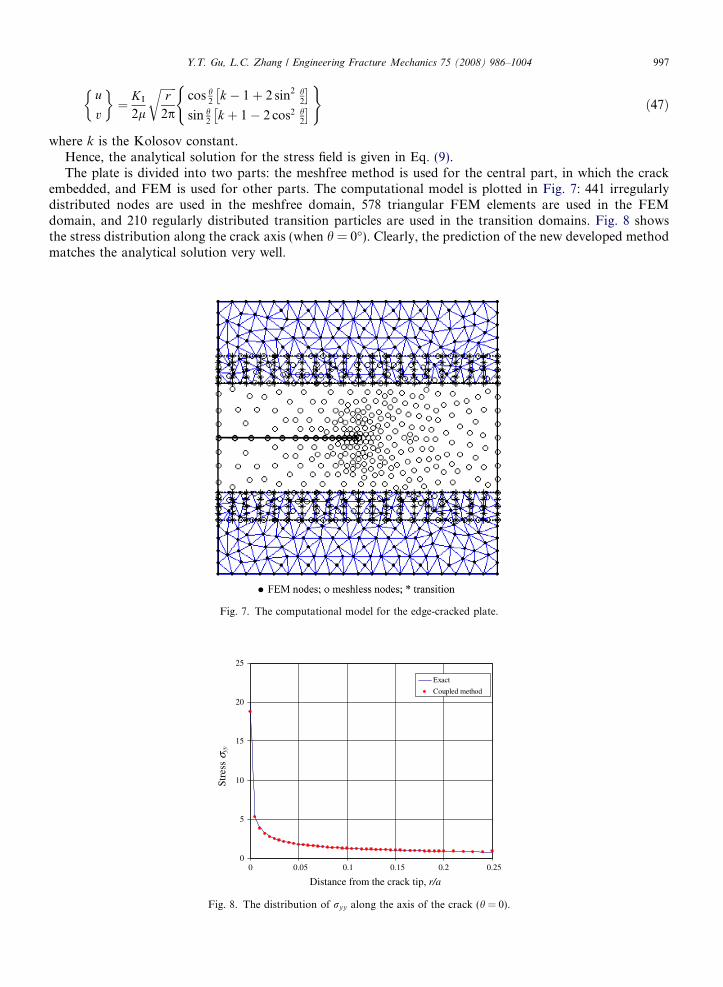
where k is the Kolosov constant.Hence, the analytical solution for the stress field is given in Eq. (9).The plate is divided into two parts: the meshfree method is used for the central part, in which the crack

embedded, and FEM is used for other parts. The computational model is plotted in Fig. 7: 441 irregularlydistributed nodes are used in the meshfree domain, 578 triangular FEM elements are used in the FEMdomain, and 210 regularly distributed transition particles are used in the transition domains. Fig. 8 showsthe stress distribution along the crack axis (when h = 0�). Clearly, the prediction of the new developed methodmatches the analytical solution very well.

Fig. 7. The computational model for the edge-cracked plate.

0

5

10

15

20

25

0 0.05 0.1 0.15 0.2 0.25

Exact

Coupled method

Distance from the crack tip, r/a

Stre

ssσ y

y

Fig. 8. The distribution of ryy along the axis of the crack (h = 0).


It should be mentioned that the sole FEM will lead to worse accuracy for this problem, especially for thestress distributions around the crack tip, because FEM without the enriched basis function usually has badaccuracy and is difficult to capture the stress singularity near the crack tip. Although using the high-orderFEM elements can partly solve this issue, FEM still has technical difficulty for the fracture problems (espe-cially the dynamic fracture problems). It has also been proven [12] that the sole meshfree method has muchbetter accuracy for the crack problem. However, the computational efficiency will be worse if the sole meshfreemethod is used. Our studies show that the present coupled method can keep the good accuracy of the meshfreemethod for the crack tip field, and, at the same time, it can save much computational cost because of the use ofFEM in the regions far away from the crack tip.

5

10

x

y

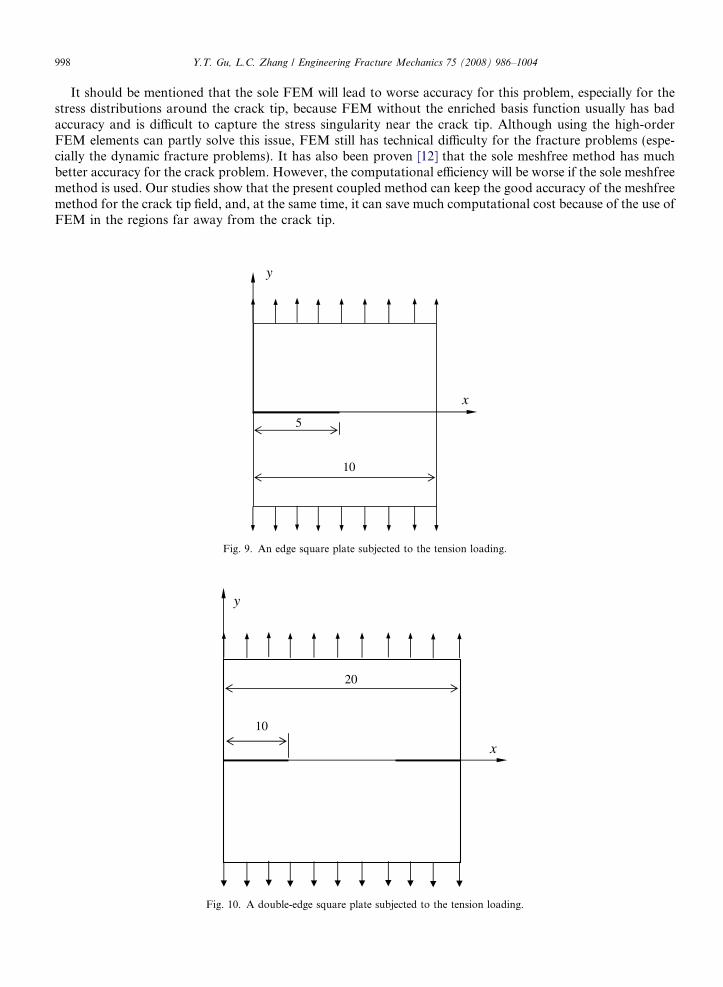
Fig. 9. An edge square plate subjected to the tension loading.

y

20

10

x

Fig. 10. A double-edge square plate subjected to the tension loading.


6.3. Two edge-cracked plates loaded in tension

An edge-cracked square plate subjected to a uniformed tension of f = 1.0, as shown in Fig. 9, is studied.The plane strain case is considered, and E = 1000, m = 0.25. The analytical results for KI had been givenby Gdoutos [28] and Ching and Batra [27]. For these parameters used here, the analytical (KI)analytical =11.2.

Fig. 11. The computational model for the plate with two edge cracks.

x

y

7

14

3.5

t=1.0

Fig. 12. An edge-cracked plate subjected to the shear loading.


The computational model is the same as that used in Section 6.2 and shown in Fig. 7. Stress intensity fac-tors were computed using the domain form of the J-integral. Our study found that the coupled method usingthe MLSA with the enriched basis functions makes the J-integral almost domain independent, given to(KI)numerical = 11.31. Compared with the analytical solution, the coupled method leads to a stable and accurateresult.

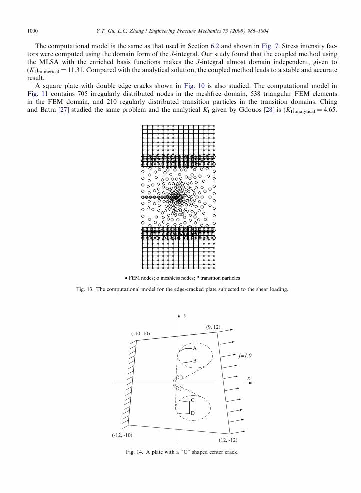
A square plate with double edge cracks shown in Fig. 10 is also studied. The computational model inFig. 11 contains 705 irregularly distributed nodes in the meshfree domain, 538 triangular FEM elementsin the FEM domain, and 210 regularly distributed transition particles in the transition domains. Chingand Batra [27] studied the same problem and the analytical KI given by Gdouos [28] is (KI)analytical = 4.65.

Fig. 13. The computational model for the edge-cracked plate subjected to the shear loading.

(-12, -10) (12, -12)

(9, 12) (-10, 10)

y

x

A

Bf=1.0

C

D

Fig. 14. A plate with a ‘‘C’’ shaped center crack.


Using the J-integral, the present coupled method gives (KI)numerical = 4.75. The coupled method leads to avery accurate result.

6.4. Shear edge crack

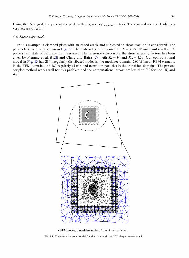
In this example, a clamped plate with an edged crack and subjected to shear traction is considered. Theparameters have been shown in Fig. 12. The material constants used are E = 3.0 · 106 units and t = 0.25. Aplane strain state of deformation is assumed. The reference solution for the stress intensity factors has beengiven by Fleming et al. ([12]) and Ching and Batra [27] with KI = 34 and KII = 4.55. Our computationalmodel in Fig. 13 has 284 irregularly distributed nodes in the meshfree domain, 280 bi-linear FEM elementsin the FEM domain, and 180 regularly distributed transition particles in the transition domains. The presentcoupled method works well for this problem and the computational errors are less than 2% for both KI andKII.

Fig. 15. The computational model for the plate with the ‘‘C’’ shaped center crack.


6.5. Cracks in a complex shaped plate

Let us now consider a plate of complex shape with a ‘‘C’’ shaped crack. The material constants used areE = 3.0 · 107 and t = 0.3. One edge of the plate is fixed, one edge is subjected to uniformly distributed tensionload, and the rest edges are traction free. As shown in Fig. 14, the plate is divided into two parts. The meshfreemethod is used in the central part including the crack, and FEM is used for other parts. The computationalmodel shown in Fig. 15 contains 595 irregularly distributed nodes in the meshfree domain, 660 triangularFEM elements in the FEM domain, and 560 regularly distributed transition particles in the transitiondomains. As a reference solution, this problem is also analyzed by the sole meshfree method (the softwareof MFree 2D: Liu [20]) with very fine nodal distribution. Fig. 16 shows the distribution of stress, rxx, obtainedby the present coupled method. It is almost identical with the meshfree method result. Table 1 lists the com-parison of displacements and stress of four points shown in Fig. 14.

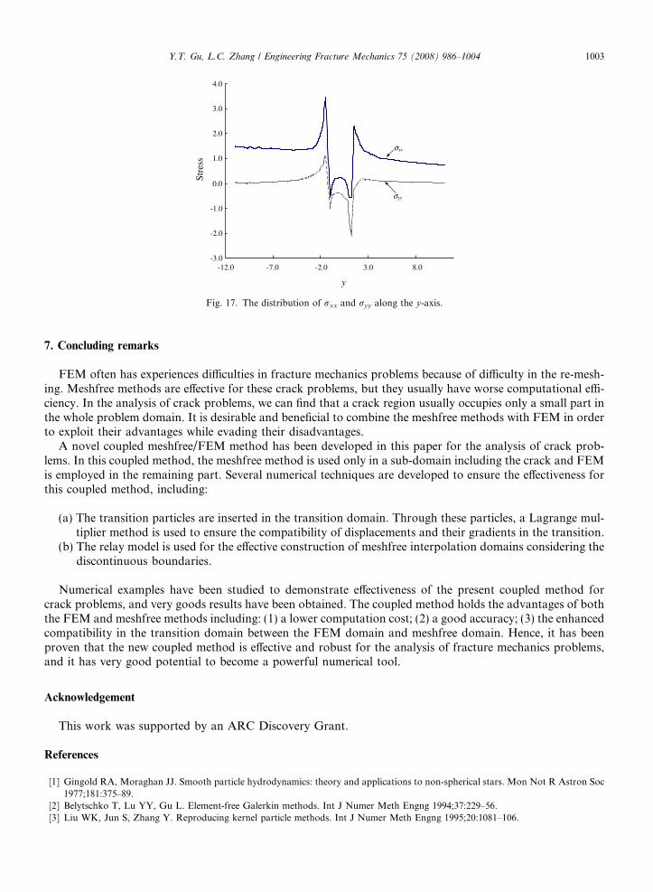
Fig. 17 shows the stress distribution along y-axis, and, again, very good agreement is obtained between thecoupled method and the purely meshfree method. The stress concentrations on the crack tips have been clearlyshown with the stress concentration factor around 3.3.

It should be mentioned here that for this problem, the coupled method uses less computational cost thanthe pure meshfree method, because we only apply the meshfree method in a very small region (about 10%of the problem domain) and FEM is used in the other area when FEM has a better computational efficiencythan the meshfree method (Liu and Gu [13]). Hence, the advantage of the present coupled method has beenproven by this example.

Fig. 16. The distribution of rxx.

Table 1The displacements and stresses for four points in this plate

Displacement Stress

u (·10�7) v (·10�7) rxx ryy sxy

Point A MFree 2D 4.1 3.4 2.31 �0.02 �0.03The coupled method 3.9 3.2 2.27 �0.017 �0.028

Point B MFree 2D 4.9 2.8 �0.57 �1.6 �0.45The coupled method 4.7 2.9 �0.61 �1.72 �0.55

Point C MFree 2D 5.3 4.2 �0.56 �1.05 0.36The coupled method 5.2 4.0 �0.54 �1.01 0.32

Point D MFree 2D 4.5 4.3 3.51 1.13 1.37The coupled method 4.2 4.2 3.34 1.08 1.32

-3.0

-2.0

-1.0

0.0

1.0

2.0

3.0

4.0

-12.0 -7.0 -2.0 3.0 8.0

σxx

σyy

y

Stre

ss

Fig. 17. The distribution of rxx and ryy along the y-axis.


7. Concluding remarks

FEM often has experiences difficulties in fracture mechanics problems because of difficulty in the re-mesh-ing. Meshfree methods are effective for these crack problems, but they usually have worse computational effi-ciency. In the analysis of crack problems, we can find that a crack region usually occupies only a small part inthe whole problem domain. It is desirable and beneficial to combine the meshfree methods with FEM in orderto exploit their advantages while evading their disadvantages.

A novel coupled meshfree/FEM method has been developed in this paper for the analysis of crack prob-lems. In this coupled method, the meshfree method is used only in a sub-domain including the crack and FEMis employed in the remaining part. Several numerical techniques are developed to ensure the effectiveness forthis coupled method, including:

(a) The transition particles are inserted in the transition domain. Through these particles, a Lagrange mul-tiplier method is used to ensure the compatibility of displacements and their gradients in the transition.

(b) The relay model is used for the effective construction of meshfree interpolation domains considering thediscontinuous boundaries.

Numerical examples have been studied to demonstrate effectiveness of the present coupled method forcrack problems, and very goods results have been obtained. The coupled method holds the advantages of boththe FEM and meshfree methods including: (1) a lower computation cost; (2) a good accuracy; (3) the enhancedcompatibility in the transition domain between the FEM domain and meshfree domain. Hence, it has beenproven that the new coupled method is effective and robust for the analysis of fracture mechanics problems,and it has very good potential to become a powerful numerical tool.

Acknowledgement

This work was supported by an ARC Discovery Grant.

References

[1] Gingold RA, Moraghan JJ. Smooth particle hydrodynamics: theory and applications to non-spherical stars. Mon Not R Astron Soc1977;181:375–89.

[2] Belytschko T, Lu YY, Gu L. Element-free Galerkin methods. Int J Numer Meth Engng 1994;37:229–56.[3] Liu WK, Jun S, Zhang Y. Reproducing kernel particle methods. Int J Numer Meth Engng 1995;20:1081–106.


[4] Liew KM, Wu YC, Zou GP, Ng TY. Elasto-plasticity revisited: numerical analysis via reproducing kernel particle method andparametric quadratic programming. Int J Numer Meth Engng 2002;55:669–83.

[5] Atluri SN, Shen SP. The meshfree local Petrov–Galerkin (MLPG) method. Tech Science Press. Encino, USA, 2002.[6] Atluri SN, Zhu T. A new meshfree local Petrov–Galerkin (MLPG) approach in computational mechanics. Computational Mechanics

1998;22:117–27.[7] Gu YT, Liu GR. A meshfree local Petrov–Galerkin (MLPG) method for free and forced vibration analyses for solids. Comput Mech

2001;27(3):188–98.[8] Gu YT, Liu GR. A local point interpolation method for static and dynamic analysis of thin beams. Comput Method Appl M

2001;190:5515–28.[9] Liu GR, Gu YT. A local radial point interpolation method (LR-PIM) for free vibration analyses of 2-D solids. J Sound Vib

2001;246(1):29–46.[10] Wang QX, Lam KY, et al. Analysis of microelectromechanical systems (MEMS) by meshless local Kriging (LoKriging) method. J

Chinese Inst Engineers 2003;27(4):573–83.[11] Liew KM, Chen XL. Mesh-free radial point interpolation method for the buckling analysis of Mindlin plates subjected to in-plane

point loads. Int J Numer Meth Engng 2004;60(11):1861–77.[12] Fleming M, Chu Y, Moran B, Belytschko T. Enriched element-free Galerkin methods for crack tip fields. Int J Numer Meth Engng

1997;40:1483–504.[13] Liu GR, Gu YT. An introduction to meshfree methods and their programming. Berlin: Springer; 2005.[14] Belytschko T, Organ D. Coupled finite element–element-free Galerkin method. Comput Mech 1995;17:186–95.[15] Hegen D. Element-free Galerkin methods in combination with finite element approaches. Comput Meth Appl Mech. Engng

1996;135:143–66.[16] Gu YT, Liu GR. A coupled element free Galerkin/boundary element method for stress analysis of two-dimensional solids. Comput

Meth Appl Mech. Engng 2001;190/34:4405–19.[17] Gu YT, Liu GR. Hybrid boundary point interpolation methods and their coupling with the element free Galerkin method. Engng

Anal Bound Elem 2003;27(9):905–17.[18] Liu GR, Gu YT. Meshfree local Petrov–Galerkin (MLPG) method in combination with finite element and boundary element

approaches. Comput Mech 2000;26(6):536–46.[19] Gu YT, Liu GR. Meshfree methods coupled with other methods for solids and structures. Tsinghua Science and Technology

2005;10(1):8–15.[20] Liu GR. Mesh free methods: moving beyond the finite element method. USA: CRC Press; 2002.[21] Anderson TL. Fracture mechanics: fundamental and applications. 1st ed. CRC Press; 1991.[22] Zienkiewicz OC, Taylor RL. The finite element method. 5th ed. Oxford, UK: Butterworth Heinemann; 2000.[23] Gu YT, Zhang LC. A concurrent multiscale method for structures based on the combination of the meshfree method and the

molecular dynamics. Multiscale Modeling and Simulation: A SIAM Interdisciplinary Journal 2006;5(4):1128–55.[24] Organ DJ, Fleming M, Belytschko T. Continuous meshfree approximations for nonconvex bodies by diffraction and transparency.

Comput Mech 1996;18:225–35.[25] Liu GR, Tu ZH. An adaptive procedure based on background cells for meshfree methods. Comput Meth Appl Mech Engng

2002;191:1923–43.[26] Timoshenko SP, Goodier JN. Theory of elasticity. 3rd ed. New York: McGraw-hill; 1970.[27] Ching HK, Batra RC. Determination of crack tip fields in linear elastostatics by the meshfree local Petrov–Galerkin (MLPG)

method. CMES 2001;l2(2):273–89.[28] Gdoutos EE. Fracture mechanics: an introduction. Kluwer Academic Publishers; 1993.

coupling of the meshfree and ﬁnite element methods for determination of ... · coupling of the...

Documents