Course notes for csc 165 h:

Mathematical Expression and Reasoningfor Computer Science

Fall 2013

Gary Baumgartner Danny Heap Richard Krueger Fran�cois Pitt

Department of Computer Science

University of Toronto

These notes are licensed under a Creative Commons

Attribution, Non-Commercial, No Derivatives 3.0 Unported License.

You may copy, distribute, and transmit these notes for free and without seeking

speci�c permission from the authors, as long as you attribute the work to its authors,

you do not use it for commercial purposes, and you do not alter it in any way.

Any other use of these notes requires the express written permission of the authors.

Visit http://creativecommons.org/licenses/by-nc-nd/3.0/ for full details.

Copyright c 2013 by Gary Baumgartner, Danny Heap, Fran�cois Pitt

Course notes for csc 165 h

2

Contents

1 Introduction 5

1.1 What's csc 165 h about? . . . . . . . . . . . . . . . . . . . . . . . . . . . . . . . . . . . . . . 5

1.2 Human versus technical communication . . . . . . . . . . . . . . . . . . . . . . . . . . . . . . 7

1.3 Problem-solving . . . . . . . . . . . . . . . . . . . . . . . . . . . . . . . . . . . . . . . . . . . . 8

1.4 Inspirational puzzles . . . . . . . . . . . . . . . . . . . . . . . . . . . . . . . . . . . . . . . . . 9

1.5 Some mathematical prerequisites . . . . . . . . . . . . . . . . . . . . . . . . . . . . . . . . . . 10

2 Logical Notation 15

2.1 Universal quanti�cation . . . . . . . . . . . . . . . . . . . . . . . . . . . . . . . . . . . . . . . 15

2.2 Existential quanti�cation . . . . . . . . . . . . . . . . . . . . . . . . . . . . . . . . . . . . . . 16

2.3 Properties, sets, and quanti�cation . . . . . . . . . . . . . . . . . . . . . . . . . . . . . . . . . 16

2.4 Sentences, statements, and predicates . . . . . . . . . . . . . . . . . . . . . . . . . . . . . . . 18

2.5 Implications . . . . . . . . . . . . . . . . . . . . . . . . . . . . . . . . . . . . . . . . . . . . . . 19

2.6 Quanti�cation and implication together . . . . . . . . . . . . . . . . . . . . . . . . . . . . . . 22

2.7 Vacuous truth . . . . . . . . . . . . . . . . . . . . . . . . . . . . . . . . . . . . . . . . . . . . . 23

2.8 Equivalence . . . . . . . . . . . . . . . . . . . . . . . . . . . . . . . . . . . . . . . . . . . . . . 23

2.9 Restricting domains . . . . . . . . . . . . . . . . . . . . . . . . . . . . . . . . . . . . . . . . . 24

2.10 Conjunction (And) . . . . . . . . . . . . . . . . . . . . . . . . . . . . . . . . . . . . . . . . . . 24

2.11 Disjunction (Or) . . . . . . . . . . . . . . . . . . . . . . . . . . . . . . . . . . . . . . . . . . . 24

2.12 Negation . . . . . . . . . . . . . . . . . . . . . . . . . . . . . . . . . . . . . . . . . . . . . . . . 25

2.13 Symbolic grammar . . . . . . . . . . . . . . . . . . . . . . . . . . . . . . . . . . . . . . . . . . 26

2.14 Truth tables . . . . . . . . . . . . . . . . . . . . . . . . . . . . . . . . . . . . . . . . . . . . . . 27

2.15 Tautology, satis�ability, unsatis�ability . . . . . . . . . . . . . . . . . . . . . . . . . . . . . . . 27

2.16 Logical \arithmetic" . . . . . . . . . . . . . . . . . . . . . . . . . . . . . . . . . . . . . . . . . 28

2.17 Summary of manipulation rules . . . . . . . . . . . . . . . . . . . . . . . . . . . . . . . . . . . 29

2.18 Multiple quanti�ers . . . . . . . . . . . . . . . . . . . . . . . . . . . . . . . . . . . . . . . . . . 30

2.19 Mixed quanti�ers . . . . . . . . . . . . . . . . . . . . . . . . . . . . . . . . . . . . . . . . . . . 30

3 Proofs 33

3.1 What is a proof? . . . . . . . . . . . . . . . . . . . . . . . . . . . . . . . . . . . . . . . . . . . 33

3.2 Direct proof of universally-quanti�ed implication . . . . . . . . . . . . . . . . . . . . . . . . . 34

3.3 An odd example of direct proof . . . . . . . . . . . . . . . . . . . . . . . . . . . . . . . . . . . 35

3.4 Indirect proof of universally-quanti�ed implication . . . . . . . . . . . . . . . . . . . . . . . . 37

3.5 Direct proof of universally-quanti�ed predicate . . . . . . . . . . . . . . . . . . . . . . . . . . 37

3.6 Proof by contradiction . . . . . . . . . . . . . . . . . . . . . . . . . . . . . . . . . . . . . . . . 37

3.7 Direct proof structure of the existential . . . . . . . . . . . . . . . . . . . . . . . . . . . . . . 38

3.8 Multiple quanti�ers, implications, and conjunctions . . . . . . . . . . . . . . . . . . . . . . . . 38

3.9 Example of proving a statement about a sequence . . . . . . . . . . . . . . . . . . . . . . . . 39

3.10 Example of disproving a statement about a sequence . . . . . . . . . . . . . . . . . . . . . . . 40

3

Course notes for csc 165 h

3.11 Non-boolean function example . . . . . . . . . . . . . . . . . . . . . . . . . . . . . . . . . . . 41

3.12 Substituting known results . . . . . . . . . . . . . . . . . . . . . . . . . . . . . . . . . . . . . 41

3.13 Proof by cases . . . . . . . . . . . . . . . . . . . . . . . . . . . . . . . . . . . . . . . . . . . . . 42

3.14 Building formulae and taking formulae apart . . . . . . . . . . . . . . . . . . . . . . . . . . . 44

3.15 Summary of inference rules . . . . . . . . . . . . . . . . . . . . . . . . . . . . . . . . . . . . . 46

4 Algorithm Analysis and Asymptotic Notation 49

4.1 Correctness, running time of programs . . . . . . . . . . . . . . . . . . . . . . . . . . . . . . . 49

4.2 Binary (base 2) notation . . . . . . . . . . . . . . . . . . . . . . . . . . . . . . . . . . . . . . . 49

4.3 Loop invariant for base 2 multiplication . . . . . . . . . . . . . . . . . . . . . . . . . . . . . . 50

4.4 Running time of programs . . . . . . . . . . . . . . . . . . . . . . . . . . . . . . . . . . . . . . 52

4.5 Linear search . . . . . . . . . . . . . . . . . . . . . . . . . . . . . . . . . . . . . . . . . . . . . 52

4.6 Run time and constant factors . . . . . . . . . . . . . . . . . . . . . . . . . . . . . . . . . . . 53

4.7 Asymptotic notation: Making Big-O precise . . . . . . . . . . . . . . . . . . . . . . . . . . . . 54

4.8 Calculus! . . . . . . . . . . . . . . . . . . . . . . . . . . . . . . . . . . . . . . . . . . . . . . . 56

4.9 Other bounds . . . . . . . . . . . . . . . . . . . . . . . . . . . . . . . . . . . . . . . . . . . . . 57

4.10 Asymptotic notation and algorithm analysis . . . . . . . . . . . . . . . . . . . . . . . . . . . . 59

4.11 Insertion sort example . . . . . . . . . . . . . . . . . . . . . . . . . . . . . . . . . . . . . . . . 60

4.12 Of algorithms and stockbrokers . . . . . . . . . . . . . . . . . . . . . . . . . . . . . . . . . . . 61

4.13 Exercises for asymptotic notation . . . . . . . . . . . . . . . . . . . . . . . . . . . . . . . . . . 64

4.14 Exercises for algorithm analysis . . . . . . . . . . . . . . . . . . . . . . . . . . . . . . . . . . . 65

4.15 Induction interlude . . . . . . . . . . . . . . . . . . . . . . . . . . . . . . . . . . . . . . . . . . 66

5 A Taste of Computability Theory 69

5.1 The problem . . . . . . . . . . . . . . . . . . . . . . . . . . . . . . . . . . . . . . . . . . . . . 69

5.2 An impossible proof . . . . . . . . . . . . . . . . . . . . . . . . . . . . . . . . . . . . . . . . . 69

5.3 Reductions . . . . . . . . . . . . . . . . . . . . . . . . . . . . . . . . . . . . . . . . . . . . . . 71

5.4 Countability . . . . . . . . . . . . . . . . . . . . . . . . . . . . . . . . . . . . . . . . . . . . . . 72

5.5 Diagonalization . . . . . . . . . . . . . . . . . . . . . . . . . . . . . . . . . . . . . . . . . . . . 75

4

Chapter 1

Introduction

1.1 What's csc 165 h about?

In addition to hacking, computer scientists have to be able to understand program speci�cations, APIs, and

their workmate's code. They also have to be able to write clear, concise documentation for others.

In our course you'll work on:

� Expressing yourself clearly (using English and mathematical expression).

� Understanding technical documents and logical expressions.

� Deriving conclusions from logical arguments, several proof techniques.

� Analyzing program e�ciency.

In this course we care about communicating precisely:

� Knowing and saying what you mean.

� Understanding what others say and mean.

We want this course to help you during your university career whenever you need to read and understand

technical material|course textbooks, assignment speci�cations, etc.

Who needs csc 165 h?

You need this course if you do:

memorize math;

have trouble explaining what you are doing in a mathematical or technical question;

have trouble understanding word problems.

You need this course if you don't:

like reading math textbooks to learn new math;

enjoy talking about abstract x and y just as much as when concrete examples are given for x and y;

have a credit for csc 238 h in your academic history, or intend to take csc 240 h.

5

Course notes for csc 165 h

Why does CS need mathematical expressions and reasoning?

We all enjoy hacking, that is designing and implementing interesting algorithms on computers. Perhaps

not all of us associate this with the sort of abstract thinking and manipulation of symbols associated with

mathematics. However there is a useful two-way contamination between mathematics and computer science.

Here are some examples of branches of mathematics that taint particular branches of Computer Science:

Computer graphics use multi-variable calculus, projective geometry, linear algebra, physics-based mod-

elling

Numerical analysis uses multivariable calculus and linear algebra

Cryptography uses number theory, �eld theory

Networking uses graph theory, statistics

Algorithms use combinatorics, probability, set theory

Databases use set theory, logic

AI uses set theory, probability, logic

Programming languages use set theory, logic

How to do well in csc 165 h

Check the course web page and the course forum frequently.

Understand the course information sheet. This is the document that we are committed to live by in this

course.

Get in the habit of asking questions and contributing to the answers.

Spend time on this course. The model that we instructors assume is that you work an average of 8{10 hours

per week on this course (3{4 in lecture and tutorial, and 5{6 reviewing notes, working on assigned

problems, attending o�ce hours (as required), etc.) Any material that's new to you will require time

for you to really acquire it and use it on other courses.

Don't plagiarize. Passing o� someone else's work as your own is an academic o�ense. Always give

generous and complete credit when you consult other sources (books, web pages, other students).

About these notes

These notes were originally created by Gary Baumgartner (and contributed to by many others), expanded

and typeset by Danny Heap and Richard Krueger, and further expanded and modi�ed by Fran�cois Pitt.

These notes are written to stand alone and cover the material included in the present csc 165 h syllabus

without the need of a supplementary textbook (though it's often advantageous to read another perspective).

Please let us know of any typos or errors, or anything that seems (unintentionally) confusing on the �rst

read, so we can make appropriate corrections.

In these notes you'll �nd numerous superscripts.1 These often indicate answers to questions worked out

in lecture, and through the wonders of word processing, those answers are formatted as endnotes (at the end

of the chapter). Our motivation isn't so much to give you whiplash moving your gaze between the question

and the answer, as to allow you to form your own answer before looking at our version.

6

Chapter 1. Introduction

1.2 Human versus technical communication

Natural languages (English, Chinese, Arabic, for example) are rich and full of potential ambiguity. In many

cases humans speaking these languages share a lot of history, context, and assumptions that remove or

reduce the ambiguity. If we don't share (or choose to momentarily forget) the history and context, there

is a rich source of humour in double-meanings created by natural languages. For example, consider these

headlines listed on http://www.departments.bucknell.edu/linguistics/semhead.html:

Prostitutes appeal to Pope

Iraqi head seeks arms

Police begin campaign to run down jay-walkers

Death may cause loneliness, feelings of isolation

Two sisters reunite after 18 years at checkout counter.2

Computers are notorious for lacking a sense of humour, and we communicate with them using extremely con-

strained languages called programming languages. In programming languages, expressions aren't expected

to be ambiguous.

Human technical communication about computing must be similarly constrained. We have to assume

less common history and context is shared with the other humans participating in technical communication,

and misplaced assumptions can result in catastrophe. We aim for increased precision, that is a smaller

tolerance for ambiguity. We will use mathematical logic, a precise language, as a form of communication

in this course.

Mathematicians share a common dialect to talk unambiguously about particular concepts in their work

(e.g., \di�erentiable functions are continuous"). Often ordinary words (\continuous") are used with re-

stricted, or special, meanings. The same word may have di�erent technical meaning in di�erent mathe-

matical contexts, for example group may mean one thing in group theory, another in combinatorial design

theory.

Since technical language is used between human beings, some degree of ambiguity is tolerated, and

probably necessary. For example, an audience of Java programmers would not object to the subtle shift in

the meaning used for \a" in the following fragments:3

/** Sorts a in ascending order */

public void sort(int[] a) ...

versus

// sets a to 1

a = 1;

Since another human is reading our comments, this potential for double meaning is benign. A computer

reading our comments would, of course, be unforgiving. However, Java programmers have to assume famil-

iarity with programming from their audience, to avoiding driving others crazy by writing long comments

(and being driven crazy by long comments written by others).

In this course we can't assume the context necessary to always conclude that you know what you're

saying, so you'll have to demonstrate it explicitly. On the other hand, you will learn to understand somewhat

imprecise statements that can be made precise from the context.

7

Course notes for csc 165 h

1.3 Problem-solving

Of course, as a computer scientist you are expected to do more than express yourself clearly about the

algorithms, methods, and classes that you either develop or use. You must also work on solving new and

challenging problems, sometimes without even knowing in advance whether a solution is possible. You will

learn to balance insights that may not be fully articulate, with rigour that convinces yourself and others

that your insights are correct. You need both pieces to succeed.

We will try to teach some techniques that increase your chances of gaining insight into mathematical

problems that you encounter for the �rst time. Although these techniques aren't guaranteed to succeed for

every mathematical problem, they work often enough to be useful.

Much of our approach is based on George Polya's in \How to Solve it," and other books following that

approach. Although you can �nd lots of references to this on the web, here's a pr�ecis of Polya's approach:

Understand the problem: Make sure you know what is being asked, and what information you've been

given. It helps to re-state the problem (sometimes several times) in your own words, perhaps repre-

senting it in di�erent ways or drawing some diagrams.

Plan a solution: Perhaps you've seen a similar problem. You might be able to use either its result, or the

method of solving it. Try working backwards: assume you've solved the problem and try to deduce

the next-to-last step in solving it. Try solving a simpler version of the problem, perhaps solving small

or particular cases.

Carry out your plan: See whether your plan for a solution leads somewhere. It may be necessary to

repeat parts of the earlier steps. When you're stuck, try to articulate exactly what you're missing.

Review any solution you achieve: Look back on any pieces of the puzzle you solve, try to remember

what lead to breakthroughs and what blocked progress. Carefully test your solution until you're

convinced (and can convince a skeptical peer) that you've got a solution. Extend the solved problem

to new problems.

Notice how these steps di�er from our usual pattern of either avoiding work on a problem (staring at a blank

page), or diving in without a plan. The very idea of separating the plan for �nding a solution from the act

of �nding a solution seems weird and unnatural. We'll add a further unnatural suggestion: you should keep

a record (notes or a journal) of your problem-solving attempts. This turns out to be useful both in solving

the problem at hand and later, related problems.

Here's an example of a real-life problem (eavesdropping on a streetcar) that you might apply Polya's

approach to. You're swinging from the grip on a streetcar during rush hour, and you hear the following

conversation fragments behind you, between persons A and B:

Person A: I haven't seen you in ages! How old are your three kids now?

Person B: The product of their ages (in years) is 36. [You begin to suspect that B is a di�cult conversation

partner].

Person A: That doesn't really answer my question. . .

Person B: Well, the sum of their ages (in years) is| [at this point a �re engine goes by and obscures the

rest of the answer].

Person A: That still doesn't really tell me how old they are.

Person B: Well, the eldest plays piano.

Person A: Okay, I see, so their ages are| [at this point you have to get o�, and you miss the answer].

8

Chapter 1. Introduction

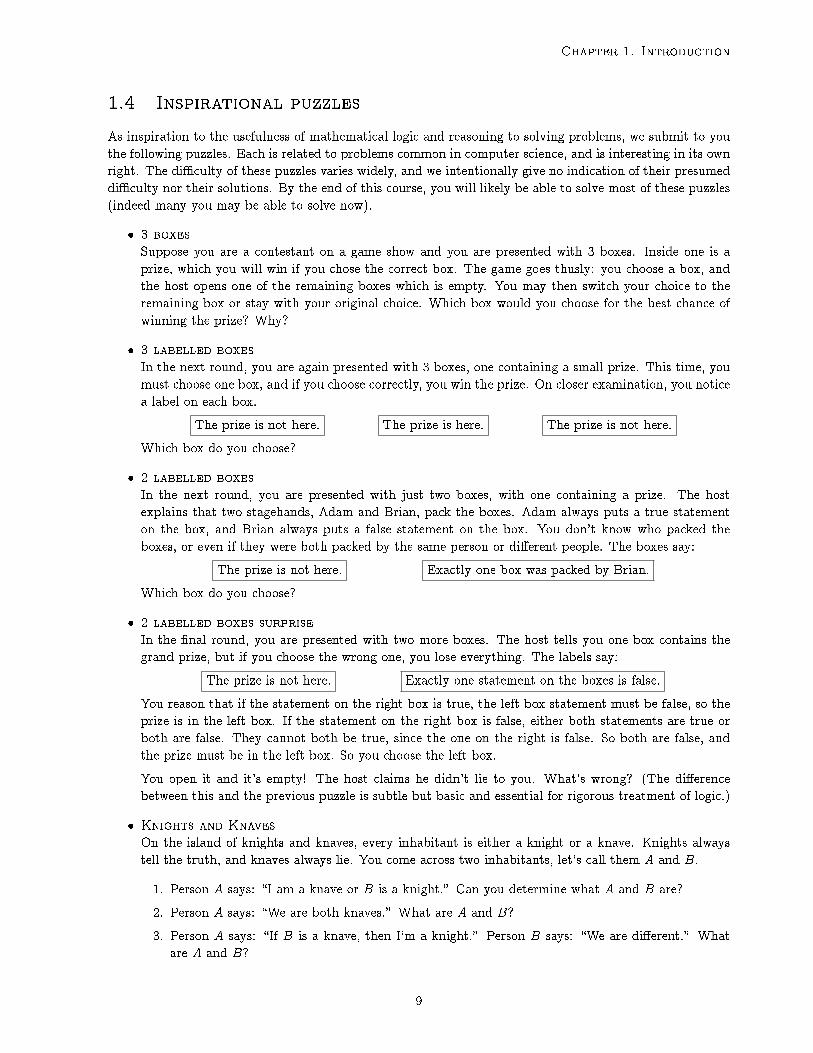
1.4 Inspirational puzzles

As inspiration to the usefulness of mathematical logic and reasoning to solving problems, we submit to you

the following puzzles. Each is related to problems common in computer science, and is interesting in its own

right. The di�culty of these puzzles varies widely, and we intentionally give no indication of their presumed

di�culty nor their solutions. By the end of this course, you will likely be able to solve most of these puzzles

(indeed many you may be able to solve now).

� 3 boxes

Suppose you are a contestant on a game show and you are presented with 3 boxes. Inside one is a

prize, which you will win if you chose the correct box. The game goes thusly: you choose a box, and

the host opens one of the remaining boxes which is empty. You may then switch your choice to the

remaining box or stay with your original choice. Which box would you choose for the best chance of

winning the prize? Why?

� 3 labelled boxes

In the next round, you are again presented with 3 boxes, one containing a small prize. This time, you

must choose one box, and if you choose correctly, you win the prize. On closer examination, you notice

a label on each box.

The prize is not here. The prize is here. The prize is not here.

Which box do you choose?

� 2 labelled boxes

In the next round, you are presented with just two boxes, with one containing a prize. The host

explains that two stagehands, Adam and Brian, pack the boxes. Adam always puts a true statement

on the box, and Brian always puts a false statement on the box. You don't know who packed the

boxes, or even if they were both packed by the same person or di�erent people. The boxes say:

The prize is not here. Exactly one box was packed by Brian.

Which box do you choose?

� 2 labelled boxes surprise

In the �nal round, you are presented with two more boxes. The host tells you one box contains the

grand prize, but if you choose the wrong one, you lose everything. The labels say:

The prize is not here. Exactly one statement on the boxes is false.

You reason that if the statement on the right box is true, the left box statement must be false, so the

prize is in the left box. If the statement on the right box is false, either both statements are true or

both are false. They cannot both be true, since the one on the right is false. So both are false, and

the prize must be in the left box. So you choose the left box.

You open it and it's empty! The host claims he didn't lie to you. What's wrong? (The di�erence

between this and the previous puzzle is subtle but basic and essential for rigorous treatment of logic.)

� Knights and Knaves

On the island of knights and knaves, every inhabitant is either a knight or a knave. Knights always

tell the truth, and knaves always lie. You come across two inhabitants, let's call them A and B.

1. Person A says: \I am a knave or B is a knight." Can you determine what A and B are?

2. Person A says: \We are both knaves." What are A and B?

3. Person A says: \If B is a knave, then I'm a knight." Person B says: \We are di�erent." What

are A and B?

9

Course notes for csc 165 h

4. You ask A: \Are you both knights?" A answers either Yes or No, but you don't know enough to

solve the problem. You then ask B: \Are you both knaves?" B answers either Yes or No, and

now you know the answer. What are A and B?

5. A and B are guarding two doors, one leading to treasure and one leading to a ferocious lion which

will surely eat you. You must choose one door. You may ask one guard one yes/no question

before choosing a door. What question do you ask? Is it easier if you know one is a knight and

one is a knave (but you don't know which is which)?

� Mother Eve

Theorem: There is a woman on Earth such that if she becomes sterile, the whole human race will die

out because all women will become sterile.

Proof: Either all women will become sterile or not. If yes, then any woman satis�es the theorem. If no,

then there is some woman that does not become sterile. She is then the one such that if she becomes

sterile (but she does not), the whole human race will die out.

Is this argument convincing?

� Santa Claus

Wife: Santa Claus exists, if I am not mistaken.

Husband: Well of course Santa Claus exists, if you are not mistaken.

Wife: Hence my statement is true.

Husband: Of course!

Wife: So I was not mistaken, and you admitted that if I was not mistaken, then Santa Claus exists.

Therefore Santa Claus exists.

Are you convinced? Why or why not?

� Daemon in a Pentagon

There is a pentagon and at each vertex there is an integer number. The numbers can be negative,

but their sum is positive. A daemon living inside the pentagon manipulates the numbers with the

following atomic action. If it spots a negative number at one of the vertices, it adds that number to its

two neighbours and negates the number at the original vertex. Prove that no matter what numbers

we start with, eventually the daemon cannot change any of the numbers.

1.5 Some mathematical prerequisites

Here are some mathematical concepts, and notation, that we'll assume you are comfortable with during this

course. We won't necessarily be teaching this material, so the onus is on you to make sure you really are

comfortable with this material and if not, to ask about it.

You may also want to refer to this section when justifying conclusions in proofs you write up for this

course.

Set theory and notation

A set is a collection of 0 or more \things". These things are called elements of the set and are often

presented as a list surrounded by curly brackets (braces), with a comma between each element.

Z: The integers, or whole numbers f: : : ;�2;�1; 0; 1; 2; : : : g.N: The natural numbers or non-negative integers f0; 1; 2; : : : g. Notice that the convention in Computer

Science is to include 0 in the natural numbers, unlike in some other disciplines.

Z+: The positive integers f1; 2; 3; : : : g.

10

Chapter 1. Introduction

Z�: The negative integers f�1;�2;�3; : : : g.Z�: The non-zero integers f: : : ;�2;�1; 1; 2; : : : g = Z� f0g = Z� [ Z+.

Q: The rational numbers (ratios of integers), comprised of f0g, Q+ (positive rationals), and Q� (negative

rationals). The set of all numbers of the form p=q, where p 2 Z and q 2 Z�.R: The real numbers, comprised of f0g, R+ (positive reals), and R� (negative reals). The set of all numbers

of the form m:d1d2d3 � � � , where m 2 Z and d1; d2; d3; : : : 2 f0; 1; 2; 3; 4; 5; 6; 7; 8; 9g.x 2 A: \x is an element of A," or \x is in A."

A � B: \A is a subset of B." Every element of A is also an element of B.

A = B: \A equals B." A and B contain exactly the same elements, in other words A � B and B � A.

A [B: \A union B." The set of elements that are in either A, or B, or both.

A \B: \A intersection B." The set of elements that are in both A and B.

A nB or A�B: \A minus B." The set of elements that are in A but not in B (the set di�erence).

jAj: \cardinality of A." The number of elements in A.

? or fg: \The empty set." A set that contains no elements. By convention, for any set A, ? � A (we will

see a logical justi�cation for this fact when we discuss vacuous truth in Section 2.7).

P(A): \The power set of A." The set of all subsets of A. For example, suppose A = f73; �g, then P(A) =f?; f73g; f�g; f73; �gg.

fx : P (x)g or fx j P (x)g: \The set of all x for which P (x) is true." For example, fx 2 Z : cos(�x) > 0g =f: : : ;�4;�2; 0; 2; 4; : : : g (even integers).

Number theory

If m and n are natural numbers, with n 6= 0, then there is exactly one pair of natural numbers (q; r) such

that:

m = qn+ r; n > r � 0:

We say that q is the quotient of m divided by n, and r is the remainder. We also say that m mod n = r.

In the special case where the remainder r is zero (so m = qn) we say that n divides m and write n j m.

We say that n is a divisor of m (e.g., 4 is a divisor of 12). Convince yourself that any natural number is a

divisor of 0, and that 1 is a divisor of any natural number.

A natural number, p, is prime if it has exactly two positive divisors. Thus 2; 3; 5; 7; 11 are all prime

but 1 is not (too few positive divisors) and 9 is not (too many positive divisors). There are in�nitely many

primes, and any integer greater than 1 can be expressed (in exactly one way) as a product of one or more

primes.

Functions

We'll use the standard notation f : A! B to say that f is a function from set A to B. In other words, for

every x 2 A there is an associated f(x) 2 B. Here are some common number-theoretic functions along with

their properties. We'll use the convention that variables x; y 2 R whereas m;n 2 Z+.

minfx; yg: \minimum of x or y." The smaller of x or y. Properties: minfx; yg � x and minfx; yg � y.

maxfx; yg: \maximum of x or y." The larger of x or y. Properties: x � maxfx; yg and y � maxfx; yg.

11

Course notes for csc 165 h

jxj: \absolute value of x," which is

(x; if x � 0

�x; if x < 0

Notice that similar notation is used for the cardinality of a set, so you have to pay attention to the

context.

gcd(m;n): \greatest common divisor of m and n." The largest positive integer that divides both m and n.

lcm(m;n): \least common multiple of m and n." The smallest positive integer that is a multiple of both m

and n. Property: gcd(m;n)� lcm(m;n) = mn.

bxc or oor(x): The largest integer that is not larger than x,

8x 2 R; y = bxc , y 2 Z ^ y � x ^ (8z 2 Z; z � x) z � y)

dxe or ceil(x): The smallest integer that is not smaller than x,

8x 2 R; y = dxe , y 2 Z ^ y � x ^ (8z 2 Z; z � x) z � y)

Inequalities

For any m;n 2 Z: m < n if and only if m+ 1 � n, and m > n if and only if m � n+ 1.

For any x; y; z; w 2 R:

� If x < y and w � z, then x+ w < y + z.

� If x < y, then

8>><>>:xz < yz if z > 0

xz = yz if z = 0

xz > yz if z < 0

� If x < y and y � z (or x � y and y < z), then x < z.

� jx+ yj � jxj+ jyj. This is an example of the triangle inequality.

Exponents and logarithms

For any a; b; c 2 R+: a = logb c if and only if ba = c.

For any x 2 R+: lnx = loge x and lg x = log2 x

For any a; b; c 2 R+ and n 2 Z+:

npb = b1=n blogb a = a = logb b

a

babc = ba+c logb(ac) = logb a+ logb c

(ba)c = bac logb(ac) = c logb a

ba=bc = ba�c logb(a=c) = logb a� logb c

b0 = 1 logb1 = 0

acbc = (ab)c

12

Chapter 1. Introduction

Chapter 1 Notes

1Like this.

2The word \appeal" in the �rst headline has two meanings, so one interpretation is that the Pope is

fond of prostitutes, and another is that prostitutes have asked the Pope for something. The words \head"

and \arms" each have two meanings, so one interpretation is that the body part above some Iraqi person's

shoulders is looking for the appendages below their shoulders, and another is that the most senior Iraqi is

looking for weapons. The phrase \run down" can mean either hitting with a car or looking for. In the fourth

headline, it's not clear to whom death causes loneliness and isolation: the dead person or their survivors. In

the �fth headline it's not clear whether the checkout line was moving really slowly, or that the checkout

counter was just the location of their reunion.

3In the �rst fragment \a" means \the object referred to by the value in a." In the second \a" means

\the variable a."

13

Course notes for csc 165 h

14

Chapter 2

Logical Notation

2.1 Universal quantification

Consider the following table that associates employees with properties:

Employee Gender Salary

Al male 60,000

Betty female 500

Carlos male 40,000

Doug male 30,000

Ellen female 50,000

Flo female 20,000

Claims about individual objects can be evaluated immediately (Al is male, Flo makes 20,000). But the

tabular form also allows claims about the entire database to be considered. For example:

Every employee makes less than 70,000.

Is this claim true? So long as we restrict our universe to the six employees, we can determine the answer.1

When a claim is made about all the objects (in this context, humans are objects!) being considered (i.e.,

in our \universe"), this is called Universal Quantification. The meaning is that we make explicit the

logical quantity (we \quantify") every member of a class or universe. English being the slippery object it is

allows several ways to say the same thing:

Each employee makes less than 70,000.

All employees make less than 70,000.

Employees make less than 70,000.2

Our universe (aka \domain") is the given set of six employees. When we say every, we mean every. This

is not always true in English, for example \Every day I have homework," probably doesn't consider the days

preceding your birth or after your death. Now consider:

Each employee makes at least 10,000.

Is this claim true? How do you know?3 A single counter-example is su�cient to refute a universally-quanti�ed

claim. What about the following claim:

All female employees make less than 55,000.

Is this claim true? Restrict the domain and check each case.4 What about

15

Course notes for csc 165 h

Every employee that earns less than 55,000 is female?5

How about this claim:

Every male employee makes less than 55,000.

It worked for females.6 Notice a pattern. To disprove a universally-quanti�ed statement you need just one

counter-example. To prove one you need to consider every element in a domain. A universally-quanti�ed

statement of the form

Every P is a Q

needs a single counter-example to disprove, and veri�cation that every element of the domain is an

example to prove.

2.2 Existential quantification

Here's another sort of claim:

Some employee earns over 57,000.

At �rst this claim doesn't seem to be about the whole database, but just about an employee who earns over

57,000 (if that employee exists, and Al does exist). But what about:

There is an employee who earns less than 57,000.

This claim is also true, and it is veri�ed by any of the employees in the set fBetty;Carlos;Doug;Ellen;Flog.It's not a claim about any particular employee in that �ve-member set, but rather a claim that the set isn't

empty. Although the non-empty set might have many members, one example of a member of the set is

enough to show that it's not empty. Now consider:

Some employee earns over 80,000.

This claim is false. There isn't an employee in the database who earns over 80,000. To show the set of

employees earning over 80,000 is empty, you have to consider every employee in the universe and demonstrate

that they don't earn over 80,000.

In everyday language existential quanti�cation is expressed as:

There [is / exists] [a / an / some / at least one] . . . [such that / for which] . . . ,

or [For] [a / an / some / at least one] . . . , . . .

Note that the English word \some" is always used inclusively here, so \some object is a P" is true if every

object is a P .

The claims are about the existence of one or more elements of a domain with some property, and

they are examples of existential quanti�cation. Existential quanti�cation requires you to exhibit just one

example of an element with the property to prove, but it requires you to consider the entire domain to

show that every element is a counter-example to disprove.

The anti-symmetry between universal and existential quanti�cation may be better understood by switch-

ing our point of view from properties to the sets of elements having those properties.

2.3 Properties, sets, and quantification

Let's look at that table again.

16

Chapter 2. Logical Notation

Employee Gender Salary

Al male 60,000

Betty female 500

Carlos male 40,000

Doug male 30,000

Ellen female 50,000

Flo female 20,000

Saying that Al is male is equivalent to saying Al belongs to the set of males. Symbolically we might write

Al 2 M or M(Al). It's useful and natural to interchange the ideas of properties and sets. If we denote the

set of employees as E, the set of female employees as F , the set of male employees as M , and the set of

employees who earn less than 55,000 as L, then we have a notation for concisely (and precisely) evaluating

claims such as M(Flo),7 or L(Carlos).8 So far the notation doesn't seem to have achieved much, but how

about:

Everything in F is also in L (in other notation, F � L)?

So our universally-quanti�ed claim that all females make less than 55,000 turns into a claim about subsets.

We already have some intuition about subsets, so let's put it to work by drawing a Venn diagram (see

Figure 2.1). Make sure you are solid on the meaning of \subset." Is a set always a subset of itself?9 Is the

empty set (the set with no elements) a subset of any set?10

Flo

Al

F

E

L

Doug

Carlos

Betty

Ellen

Figure 2.1: The only elements of F are also elements of L, so F � L. In this particular

diagram, the maximum number of regions consistent with F � L are occupied: three

out of the four regions are occupied.

Now consider the claim

Something in M is also in L: there is some male who does not earn less than 55,000

The complement of L is sometimes denoted L, and means elements that are not in L. One way to denote

\something in M is also in L" in set notation is M \ L 6= ?|saying \something" is in both sets is the

same as saying their intersection is non-empty. Now, you should be able to compare this to the de�nition

of a subset to see that this is same as saying that M is not a subset of L, or M 6� L.

The anti-symmetry of universal and existential quanti�cation becomes systematic:

� Every P is a Q means P � Q. To prove this claim you need to consider every element of P and show

they are also elements of Q. To disprove this claim, you need to �nd just one element of P that is not

an element of Q.

� Some P is a Q means P 6� Q. To prove this you need to �nd just one P that isn't a non-Q (a round-

about way of saying �nd just one P that is a Q). To disprove it, you must consider every P and show

they are also non-Qs.

17

Course notes for csc 165 h

2.4 Sentences, statements, and predicates

Recall the table of employees with their genders and salaries from above:

Employee Gender Salary

Al male 60,000

Betty female 500

Carlos male 40,000

Doug male 30,000

Ellen female 50,000

Flo female 20,000

Now consider the following claims:

Claim 2.1: The employee makes less than 55,000.

Claim 2.2: Every employee makes less than 55,000.

Can you decide whether both claims are true or false?11 The basic di�erence between the two claims

is that Claim 2.1 is about a particular employee, and it is true or false depending on the earnings of that

employee, whereas Claim 2.2 is about the entire set of employees, E, and it is true or false depending on

where that set of employees stands in relation to the set L, those who earn over 55,000.

Claim 2.1 is called a sentence. It may refer to unquanti�ed objects (for example \the employee"). Once

the objects are speci�ed (substitutions are made for the variable(s)), a sentence is either true or false (but

never both). Claim 2.2 is called a statement. It doesn't refer to any unquanti�ed variables, and it is either

true or false (never both). Every statement is a sentence, but not every sentence is a statement. If you want

to make it explicit that a sentence refers to unquanti�ed objects, you may call it an \open sentence." Thus

a sentence is a statement if and only if it is not open. Universal quanti�cation transformed Claim 2.1 into

Claim 2.2, from an open sentence about an unspeci�ed element of the set of employees, into a statement

about the (speci�ed in the database) sets of Employees and those earning over 55,000.

Symbols

Symbols are useful when they make expressions clearer and highlight patterns in similar expressions. We

already moved in the direction of making our logical expressions symbolic by naming sets E (employees), F

(females), and L (those earning less than 55,000). Naming gives us a concise expression for these sets, and it

emphasizes the similar roles these sets play. We introduce more symbolism into our sentences, statements,

and predicates now.

As a programmer you create a sentence every time you de�ne a boolean function. In logic, a predicate

is a boolean function. For convenience you can name your predicate, and you can de�ne it by showing how

it evaluates its input, using a symbol to stand for generic input. For example, if L is the set of employees

earning less than 55,000

L(x): x 2 L.

Notice how similar this is to de�ning a function in a programming language in terms of how it evaluates

its parameters. The symbol x is useful in the de�nition| it holds the parentheses, \(\ and \)", apart so

that we can see that exactly one value is needed, and it shows where to plug that value into the de�nition.

Notice that this de�nition would mean the same things if we replaced the symbol x with the symbol y or the

symbol y3. The symbol x doesn't specify any value that helps determine whether our predicate evaluates

to true or false. Our open sentence above, Claim 2.1, is equivalent to L(x)|we can't evaluate it without

substituting something from the set E for x. L(Carlos) is true, L(Al) is false.

18

Chapter 2. Logical Notation

Claim 2.2 is equivalent to \for all employees x, L(x)." The phrase \for all employees x" quanti�es the

variable x, and changes the claim from an open sentence about unspeci�ed x to a statement about sets E

and L, which were speci�ed in the database above. Of course, in this context, \employees" refers to those

in our database, and not any other employees.

We can indicate universal quanti�cation symbolically as 8, read as \for all." This makes sense if we

specify the universe (domain) from which we are considering \all" objects. With this notation, Claim 2.2

can be written

8 employees, the employee makes less than 55,000.

Things become clearer if we introduce a name for the unspeci�ed employee:

8 employees x, x makes less than 55,000.

Since this statement may eventually be embedded in some larger and more complicated structure, we can

add to the brevity and clarity by adding a bit more notation. Let E denote the set of employees, and L(x)

denote the predicate \x makes less than 55,000." Now Claim 2.2 becomes:

8x 2 E;L(x).

We can do something similar with existential quanti�cation. We can transform L(x) into a statement by

saying there is some element of E that also belongs to L:

There exist employees who earn less than 55,000.

9x 2 E;L(x).

The symbol we use for \there exists" is 9. This is a statement about the sets E and L (it says they have

a common, non-empty subset), and not a statement about individual elements of those sets. The symbol x

doesn't stand for a particular element, it rather indicates that there is at least one element common to E

and L.

2.5 Implications

Consider a claim of the form

if an employee is male, then he makes less than 55,000.

This is called an implication. It says that for employees, being male implies making less than 55,000.12

This is universal quanti�cation in disguise, since it could be accurately re-expressed as \Every male employee

earns less than 55,000," or 8x 2 E\M;L(x). Notice that the implication \males implies less than 55,000" has

the same e�ect as restricting the domain by intersecting E with M in the universally-quanti�ed statement.

However, it turns out to be convenient sometimes to keep the implication \male implies less than 55,000"

separate from the domain. In this way, we can consider the implication as part of universes other than E

(perhaps H, the set of humans, or X = fDoug;Carlosg). Separating the implication from the surrounding

universe also means we don't have to de�ne a set for each predicate, so we could have \M(x) implies L(x)"

without necessarily de�ning the sets M and L (although we could always come up with suitable de�nitions

if we needed to).

Just as with universal quanti�cation, the only way to disprove the implication \if P then Q" is to show

an instance where P is true but Q is false. If, in every possible instance, we have either not-P or Q, then

the implication \if P then Q" is true.

In the implication \if P then Q," we call P the antecedent (sometimes the assumption), and Q the

consequent (sometimes the conclusion).

Since logical implication borrows the English word \if," we need to reject some of the common English

uses of \if" that we don't mean when \if" is used in logic. In logic \if. . . then" tells you nothing about

19

Course notes for csc 165 h

causality. \If it rained yesterday, then the sun rose today," is a true implication, but the (possible) rain

didn't cause the (certain) rising of the sun. Also, when my mother told me \if you eat your vegetables, then

you can have dessert," she also meant \otherwise you'll get no dessert." In ordinary English, my mother

used \if. . . then" to mean \if and only if. . . then." In logic we use the more constrained meaning. We want

\If P then Q" to mean \Every P is a Q."

What does \every P is a Q" tell us? In our database example:

Claim 2.3: If an employee is female, then she makes less than 55,000.

Claim 2.3 discusses three sets, E, the set of employees, F , the set of female employees, and L, the set of

employees making less than 55,000. Claim 2.3 implicitly invokes universal quanti�cation, so it is more than

a claim about a particular employee. The Venn diagram Figure 2.1 indicates the situation corresponding to

our table. If you had no access to either the table or the Venn diagram, but only knew the Claim 2.3 was

true, what would you know about

1. F , the set of female employees? What else does the implication tell you about Ellen if you only know

that Ellen is female?

2. L, the set of employees earning less than 55,000? What do you know about Betty (if you only know

she's in L) or Carlos (if you only know he's in L)?

3. F , the set of male employees? Think about both Doug and Al.

4. L (the complement of L), the set of employees making 55,000 or more.

Knowing \P implies Q" tells us nothing more about some sets,13 however it does tell us more about others.14

Suppose you have a new employee Grn x (from a domain short of vowels), plus our Venn diagram (2.1).

Which region of the Venn diagram would you add Grn x to in order to make Claim 2.3 false?15 Once that

region is occupied, does it matter whether any of the other regions are occupied or not?16

More symbols

We can write implication symbolically as), read \implies." Now \P implies Q" becomes P)Q. Claim 2.3

could now be re-written as

an employee is female ) that employee makes less than 55,000.

Contrapositive

The contrapositive of P )Q is :Q):P (: is the symbol for negation). In English the contrapositive

of \all P is/are Q" is \all non-Q is/are non-P ." Put another way, the contrapositive of \P implies Q" is

\non-Q implies non-P ." The contrapositive of Claim 2.3 is

an employee doesn't make less than 55,000 ) that employee is not female.

or, given the structure of the domain E of employees:

an employee makes at least 55,000 ) that employee is male.

Does the contrapositive of Claim 2.3 tell us everything that Claim 2.3 itself does? Check the Venn diagram

(2.1). Does every Venn diagram that doesn't contradict Claim 2.3 also not contradict the contrapositive of

Claim 2.3?17 Can you apply the contrapositive twice? To do this it helps to know that applying negation

(:) twice toggles the truth value twice (I'm not not going means I'm going). Thus the contrapositive of the

contrapositive of P )Q is the contrapositive of :Q):P , which is ::P )::Q, equivalent to P )Q.

20

Chapter 2. Logical Notation

Converse

The converse of P)Q is Q)P . In words, the converse of \P implies Q" is \Q implies P ." An implication

and its converse don't mean the same thing. Consider the Venn diagram Figure 2.1. Would it work as a

Venn diagram for L) F?18

Consider an example where the (implicit) domain is the set of pairs of numbers, perhaps R� R.Claim 2.4: x = 1) xy = y

� If we know x = 1, then we know xy = y.

� If we know x 6= 1, then we don't know whether or not xy = y.

� If we know xy = y, then we don't know whether or not x = 1.

� If we know xy 6= y, then we know x 6= 1.

The contrapositive of Claim 2.4 is:

xy 6= y) x 6= 1.

Check the four points we knew from Claim 2.4, and see whether we know the same ones from the contra-

positive (it may be helpful to read them in reverse order). What about the converse?

xy = y) x = 1

with equivalent contrapositive

x 6= 1) xy 6= y.

The converse of Claim 2.4 is not equivalent to Claim 2.4, for example consider the pair (5; 0), that is x = 5

and y = 0. Indeed, Claim 2.4 is true, while its converse is false.

Implication in everyday English

Here are some ways of saying \P implies Q" in everyday language. In each case, try to think about what is

being quanti�ed, and what predicates (or perhaps sets) correspond to P and Q.

� If P , [then] Q.

\If nominated, I will not stand."

\If you think I'm lying, then you're a liar!"

� When[ever] P , [then] Q.

\Whenever I hear that song, I think about ice cream."

\I get heartburn whenever I eat supper too late."

� P is su�cient/enough for Q

\Di�erentiability is su�cient for continuity."

\Matching �ngerprints and a motive are enough for guilt."

� Can't have P without Q

\There are no rights without responsibilities."

\You can't stay enrolled in csc 165 h without a pulse."

� P requires Q

\Successful programming requires skill."

21

Course notes for csc 165 h

� For P to be true, Q must be true / needs to be true / is necessary

\To pass csc 165 h, a student needs to get 40% on the �nal."

� P only if / only when Q

\I'll go only if you insist."

For the antecedent (P ) look for \if," \when," \enough," \su�cient." For the consequent (Q) look for

\then," \requires," \must," \need," \necessary," \only if," \when." In all cases, check whether the expected

meaning in English matches the meaning of P ) Q. In other words, you've got an implication if, in every

possible instance, either P is false or Q is true.

2.6 Quantification and implication together

So far we have considered an implication to be universal quanti�cation in disguise:

Claim 2.5: If an employee is male, then that employee makes less than 55,000.

The English inde�nite article \an" signals that this means \Every male employee makes less than 55,000,"

and this closed sentence is either true or false, depending on the domain of employees. This can be expressed

as 8x 2 E;M(x)) L(x), and we can separate the \For all employees," portion from the \if the employee

is male, then the employee makes less than 55,000," portion. Symbolically, we can think about 8x 2 E

separately from M(x))L(x), giving us some exibility about which values we might substitute for x. This

allows us to express the unquanti�ed implication:

Claim 2.6: If the employee is male, then that employee makes less than 55,000.

The English de�nite article \the" often signals an unspeci�ed value, and hence an open sentence. We could

transform Claim 2.6 back into Claim 2.5 by pre�xing it with \For every employee, . . . "

Claim 2.7: For every employee, if the employee is male, then that employee makes less than 55,000.

Since the claim is about male employees, we are tempted to say 8m 2 M;L(m), which would be correct

if the only males we were considering were those in E| 8m 2 E \M;L(m) would certainly capture what

we mean. Using that approach we would restrict the domain that we are universally quantifying over by

intersecting with other domains. However, it is often convenient to restrict in another way: set our domain

to the largest universe in which the predicates make sense, and use implication to restrict further. We don't

have to avoid reasoning about non-males when we say 8e 2 E;M(e)) L(e), and we get the same meaning

as 8m 2 E \M;L(m).

It also often happens that the predicate expressed by M(e) doesn't neatly translate into a set that can

be intersected with set E, so the universally quanti�ed implication format can be handy. For example,

8n 2 N; n > 0) 1=n 2 R means the same things as 8n 2 N n f0g; 1=n 2 R, but expressing the set N n f0gseems more awkward than using universally-quanti�ed implication, and there are much worse cases.

How do you feel about verifying Claim 2.6 for all six values in E, which are true/false?19

Do you feel uncomfortable saying that the implications with false antecedents are true? Implications are

strange, especially when we consider them to involve causality (which we don't in logic). Consider:

Claim 2.8: If it rains in Toronto on June 2, 3007, then there are no clouds.

Is Claim 2.8 true or false? Would your answer change if you could wait the required number of decades?

What if you waited and June 2, 3007 were a completely dry day in Toronto, is Claim 2.8 true or false?20

22

Chapter 2. Logical Notation

2.7 Vacuous truth

We use the fact that the empty set is a subset of any set. Let x 2 R (the domain is the real numbers). Is

the following implication true or false?

Claim 2.9: If x2 � 2x+ 2 = 0, then x > x+ 5.

A natural tendency is to process x > x+5 and think \that's impossible, so the implication is false." However,

there is no real number x such that x2�2x+2 = 0, so the antecedent is false for every real x. Whenever the

antecedent is false and the consequent is either true or false, the implication as a whole is true. Another

way of thinking of this is that the set where the antecedent is true is empty (vacuous), and hence a subset

of every set. Such an implication is sometimes called vacuously true.

In general, if there are no P s, we consider P ) Q to be true, regardless of whether there are any Qs.

Another way of thinking of this is that the empty set contains no counterexamples. Use this sort of thinking

to evaluate the following claims:21

Claim 2.10: All employees making over 80,000 are female.

Claim 2.11: All employees making over 80,000 are male.

Claim 2.12: All employees making over 80,000 have supernatural powers and pink toenails.

2.8 Equivalence

Suppose Al quits the domain E. Consider the claim

Claim 2.13: Every male employee makes between 25,000 and 45,000.

Is Claim 2.13 true? What is its converse?22 Is the converse true? Draw a Venn diagram. The two properties

describe the same set of employees; they are equivalent. In everyday language, we might say \An employee

is male if and only if the employee makes between 25,000 and 45,000." This can be decomposed into two

statements:

Claim 2.14: An employee is male if the employee makes between 25,000 and 45,000.

Claim 2.15: An employee is male only if the employee makes between 25,000 and 45,000.

Here are some other everyday ways of expressing equivalence:

� P i� Q (\i�" being an abbreviation for \if and only if").

� P is necessary and su�cient for Q.

� P )Q, and conversely.

You may also hear

� P [exactly / precisely] when Q

For example, if our domain is R, you might say \x2 + 4x + 4 = 0 precisely when x = �2." Equivalence

is getting at the \sameness" (so far as our domain goes) of P and Q. We may de�ne properties P and

Q di�erently, but the same members of the domain have these properties (they de�ne the same sets).

Symbolically we write P ,Q. So now

An employee is male , he makes between 25,000 and 45,000.

Oddly, our (false) Claim 2.9 is an equivalence, since the implications are vacuously true in both directions:

x2 � 2x+ 2 = 0, x > x+ 5.

23

Course notes for csc 165 h

2.9 Restricting domains

Implication, quanti�cation, conjunction (\and," represented by the symbol ^), and set intersection are

techniques that can be used to restrict domains:

� \Every D that is also a P is also a Q" becomes 8x 2 D;P (x))Q(x), which we use more commonly

than the equivalent 8x 2 D \ P;Q(x)(What's the di�erence between this and 8x 2 D;P (x) ^Q(x)?)

� \Some D that is also a P is also a Q" becomes 9x 2 D;P (x) ^ Q(x), which we use more commonly

than the equivalent 9x 2 D \ P;Q(x)(What's the di�erence between this and 9x 2 D;P (x))Q(x)?)

2.10 Conjunction (And)

We use ^ (\and") to combine two sentences into a new sentence that claims that both of the original

sentences are true. In our employee database:

Claim 2.16: The employee makes less than 75,000 and more than 25,000.

Claim2.16 is true for Al (who makes 60,000), but false for Betty (who makes 500). If we identify the

sentences with predicates that test whether objects are members of sets, then the new ^ predicate tests

whether somebody is in both the set of employees who makes less than 75,000 and the set of employees who

make more than 25,000| in other words, in the intersection. Is it a coincidence that ^ resembles \ (only

more pointy)?

Notice that, symbolically, P ^ Q is true exactly when both P and Q are true, and false if only one of

them is true and the other is false, or if both are false.

We need to be careful with everyday language where the conjunction \and" is used not only to join

sentences, but also to \smear" a subject over a compound predicate. In the following sentence the subject

\There" is smeared over \pen" and \telephone:"

Claim 2.17: There is a pen and a telephone.

If we let O be the set of objects, p(x) mean x is a pen, and t(x) mean x is a telephone, then the obvious

meaning of Claim 2.17 is:23 \There is a pen and there is a telephone." But a pedant who has been observing

the trend where phones become increasingly smaller and di�cult to use might think Claim 2.17 means:24

\There is a pen-phone."

Here's another example whose ambiguity is all the more striking since it appears in a context (mathe-

matics) where one would expect ambiguity to be sharply restricted.

The solutions are:

x < 10 and x > 20

x > 10 and x < 20

The author means the union of two sets in the �rst case, and the intersection in the second. We use ^ in

the second case, and disjunction _ (\or") in the �rst case.

2.11 Disjunction (Or)

The disjunction \or" (written symbolically as _) joins two sentences into one that claims that at least one

of the sentences is true. For example,

The employee is female or makes less than 45,000.

24

Chapter 2. Logical Notation

This sentence is true for Flo (she makes 20,000 and is female) and true for Carlos (who makes less than

45,000), but false for Al (he's neither female, nor does he make less than 45,000). If we viewed this \or'ed"

sentence as a predicate testing whether somebody belonged to at least one of \the set of employees who

are female" or \the set of employees who earn less than 45,000," then it corresponds to the union. As a

mnemonic, the symbols _ and [ resemble each other. Historically, the symbol _ comes from the Latin word

\vel" meaning or.

We use _ to include the case where more than one of the properties is true; that is, we use an inclusive-

or. In everyday English we sometimes say \and/or" to specify the same thing that this course uses \or"

for, since the meaning of \or" can vary in English. The sentence \Either we play the game my way, or I'm

taking my ball and going home now," doesn't include both possibilities and is an exclusive-or: \one or the

other, but not both." An exclusive-or is sometimes added to logical systems (say, inside a computer), but

we can use negation and equivalence to express the same thing25 and avoid the complication of having two

di�erent types of \or."

2.12 Negation

We've mentioned negation a few times already, and it is a simple concept, but it's worth examining it in

detail. The negation of a sentence simply inverts its truth value. The negation of a sentence P is written as

:P , and has the value true if P was false, and has the value false if P was true.

Negation gives us a powerful way to check our determination of whether a statement is true. For example,

we can check that

Claim 2.18: All employees making over 80,000 are female.

is true by verifying that its negation is false. The negation of Claim 2.18 is

Claim 2.19: Not all employees making over 80,000 are female.

We cannot �nd any employees making over 80,000 that are not female (in fact, we cannot �nd any employees

making over 80,000 at all!), so this sentence must be false, meaning the original must be true.

You should feel comfortable reasoning about why the following are equivalent:

� :(9x 2 D;P (x) ^Q(x)),8x 2 D; (P (x)):Q(x)).In words, \No P is a Q" is equivalent to \Every P is a non-Q."

� :(8x 2 D;P (x))Q(x)),9x 2 D; (P (x) ^ :Q(x)).In words, \Not every P is a Q" is equivalent to \There is some P that is a non-Q."

Sometimes things become clearer when negation applies directly to the simplest predicates we are discussing.

Consider

Claim 2.20: 8x 2 D;9y 2 D;P (x; y)

What does it mean for Claim 2.20 to be false, i.e., :(8x 2 D;9y 2 D;P (x; y))? It means there is some x

for which the remainder of the sentence is false:

Claim 2.21: :(8x 2 D;9y 2 D;P (x; y)),9x 2 D;:(9y 2 D;P (x; y))

So now what does the negated sub-sentence mean? It means there are no y's for which the remainder of the

sentence is true:

Claim 2.22: 9x 2 D;:(9y 2 D;P (x; y)),9x 2 D;8y 2 D;:P (x; y)There is some x that for every y makes P (x; y) false. As negation (:) moves from left to right, it ips

universal quanti�cation to existential quanti�cation, and vice versa. Try it on the symmetrical counterpart

9x 2 D;8y 2 D;P (x; y), and consider

25

Course notes for csc 165 h

:(9x 2 D;8y 2 D;P (x; y)),8x 2 D;:(8y 2 D;P (x; y))

If it's not true that there exists an x such that the remainder of the sentence is true, then for all x the

remainder of the sentence is false. Considering the remaining subsentence, if it's not true that for all y the

remainder of the subsentence is true, then there is some y for which it is false:

:(9x 2 D;8y 2 D;P (x; y)),8x 2 D;9y 2 D;:P (x; y)

For every x there is some y that makes P (x; y) false.

Try combining this with implication, using the rule we discussed earlier, plus DeMorgan's law:

:(9x 2 D;8y 2 D; (P (x; y))Q(x; y))),:(9x 2 D;8y 2 D; (:P (x; y) _Q(x; y)))

2.13 Symbolic grammar

With connectives such as implication ()), conjunction (^), and disjunction (_) added to quanti�ers, you

can form very complex predicates. If you require these complex predicates to be unambiguous, it helps

to impose strict conditions on what expressions are allowed. A syntactically correct sentence is sometimes

called a well-formed formula (abbreviated w�). Note that syntactic correctness has nothing to do with

whether a sentence is true or false, or whether a sentence is open or closed. The syntax (or grammar rules)

for our symbolic language can be summarized as follows:

� Any predicate is a w�.

� If P is a w�, so is :P .� If P and Q are w�s, so is (P ^Q).� If P and Q are w�s, so is (P _Q).� If P and Q are w�s, so is (P )Q).

� If P and Q are w�s, so is (P ,Q).

� If P is a w� (possibly open in variable x) and D is a set, then (8x 2 D;P ) is a w�.

� If P is a w� (possibly open in variable x) and D is a set, then (9x 2 D;P ) is a w�.

� Nothing else is a w�.

These rules are recursive, and tell us how we're allowed to build arbitrarily complex sentences in our symbolic

language. The �rst rule is called the base case and speci�es the most basic sentence allowed. The rules

following the base case are recursive or inductive rules: they tell us how to create a new legal sentence from

smaller legal sentences. The last rule is a closure rule, and says we've covered everything.

In practice, we want to avoid writing expressions with many parentheses, so we use precedence to

disambiguate expressions that are missing parentheses. In the grammar above, precedence decreases from

top to bottom. In other words, in the absence of parentheses, parentheses must be added to sub-expressions

near the top before those near the bottom.

For example, the expression below:

8x 2 D;P (x) ^ :Q(x))R(x)

must be understood as follows|where we have indicated the order in which parentheses were put in,

according to the order of precedence above:

�48x 2 D;

�3(2P (x) ^ (1:Q(x))1)2 )R(x)

�3

�4

You should be able to convert a more loosely-structured predicate into a w�, or a w� into a more loosely-

structured predicate, whenever it's convenient.

26

Chapter 2. Logical Notation

2.14 Truth tables

Predicates evaluate to either true or false once they are completely speci�ed (all unknown values are �lled

in). If you build complex predicates from simpler ones, using connectives, it's important to know how to

evaluate the complex predicate based on the evaluation of fully-speci�ed variants of the simpler predicates

it is built out of. A powerful technique for determining the possible truth value of a complex predicate is

the use of truth tables. In a truth table, we write all possible truth values for the predicates (how many

rows do you need?26), and compute the truth value of the statement under each of these truth assignments.

Each of the logical connectives yield the following truth tables.

P :PT F

F T

P Q P ^Q P _Q P )Q P ,Q

T T T T T T

T F F T F F

F T F T T F

F F F F T T

We often break complex statements into simpler substatements, compute the truth value of the substate-

ments, and combine the truth values back into the more complex statements. For example, we can verify

the equivalence

(P ) (Q)R)), ((P ^Q))R)

using the following truth table:

P Q R Q)R P ) (Q)R) P ^Q (P ^Q))R (P ) (Q)R)), ((P ^Q))R)

T T T T T T T T

T T F F F T F T

T F T T T F T T

T F F T T F T T

F T T T T F T T

F T F F T F T T

F F T T T F T T

F F F T T F T T

Since the rightmost column is always true, our statement is a law of logic, and we can use it when manipu-

lating our symbolic statements.

2.15 Tautology, satisfiability, unsatisfiability

Notice that in the previous section, we didn't specify domains or even meanings for P or Q, nor worry about

what values might replace unspeci�ed symbols within P or Q. With truth tables we explored all possible

\worlds" (con�gurations of truth assignments to P and Q). This is known as a tautology: you can't

dream up a domain, or a meaning for predicates P and Q that provides a counter-example, since the truth

tables are identical.

This is di�erent from, say, (P )Q), (Q)P ), which will be true for some choice of domain, predicates

P and Q, and values of domain elements, so we say this statement is satisfiable. But in this case, there

are also choices of domains and/or predicates in which it is false, so it is not a tautology. Be careful: saying

that a statement is satis�able only tells us that it is possible for it to be true, without saying anything about

whether or not it is also possible for it to be false (i.e., whether or not it is also a tautology).

What about something for which no domains, predicates, or values can be chosen to make it true? Such

a statement would be unsatisfiable (or a contradiction).

27

Course notes for csc 165 h

2.16 Logical \arithmetic"

If we identify ^ and _ with set intersection and union (for the sets where the predicates they are connecting

are true), it's clear that they are associative and commutative, so

P ^Q,Q ^ P and P _Q,Q _ PP ^ (Q ^R), (P ^Q) ^R and P _ (Q _R), (P _Q) _R

Maybe a bit more surprising is that we have distributive laws for each operation over the other:

P ^ (Q _R), (P ^Q) _ (P ^R)P _ (Q ^R), (P _Q) ^ (P _R)

We can also simplify expressions using identity and idempotency laws:

identity: P ^ (Q _ :Q), P , P _ (Q ^ :Q)idempotency: P ^ P , P , P _ P

DeMorgan's Laws

These laws can be veri�ed either by a truth table, or by representing the sentences as Venn diagrams and

taking the complement.

Sentence s1 ^ s2 is false exactly when at least one of s1 or s2 is false. Symbolically:

:(s1 ^ s2), (:s1 _ :s2)

Sentence s1 _ s2 is false exactly when both s1 and s2 are false. Symbolically:

:(s1 _ s2), (:s1 ^ :s2)

By using the associativity of ^ and _, you can extend this to conjunctions and disjunctions of more than

two sentences.

Implication, bi-implication, with :;_, and ^

If we shade a Venn diagram so that the largest possible portion of it is shaded without contradicting the

implication P ) Q, we gain some insight into how to express implication in terms of negation and union.

The region that we can choose object x from so that P (x)) Q(x) is P [ Q and this easily translates to

:P _Q. This gives us an equivalence:

(P )Q), (:P _Q)Now use DeMorgan's law to negate the implication:

:(P )Q),:(:P _Q), (::P ^ :Q), (P ^ :Q)You can use a Venn diagram or some of the laws introduced earlier to show that bi-implication can be

written with ^, _, and ::(P ,Q), ((P ^Q) _ (:P ^ :Q))

DeMorgan's law tells us how to negate this:

:(P ,Q),:((P ^Q) _ (:P ^ :Q)), � � � , ((:P ^Q) _ (P ^ :Q))

28

Chapter 2. Logical Notation

Transitivity of universally-quantified implication

Consider 8x 2 D; ((P (x))Q(x))^ (Q(x))R(x))) (I have put the parentheses to make it explicit that the

implications are considered before the ^). What does this sentence imply if considered in terms of P , Q,

and R, the subsets of D where the corresponding predicates are true?27 We can also work this out using

the logical arithmetic rules we introduced above: write ((P (x))Q(x)) ^ (Q(x))R(x)))) (P (x))R(x))

using only _;^; and :, and show that it is a tautology (always true). Alternatively, use DeMorgan's law,

the distributive laws, and anything else that comes to mind to show that the negation of this sentence is a

contradiction. Thus, implication is transitive.

A similar transformation is that 8x 2 D; (P (x)) (Q(x)) R(x))), 8x 2 D; ((P (x) ^ Q(x))) R(x)).

Notice this is stronger than the previous result (an equivalence rather than an implication). This statement

can be proven with the help of truth tables.

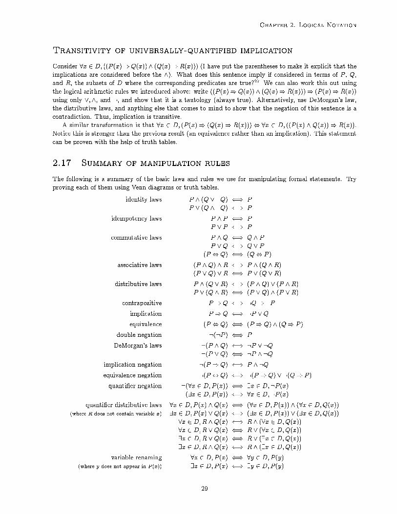
2.17 Summary of manipulation rules

The following is a summary of the basic laws and rules we use for manipulating formal statements. Try

proving each of them using Venn diagrams or truth tables.

identity laws P ^ (Q _ :Q) () P

P _ (Q ^ :Q) () P

idempotency laws P ^ P () P

P _ P () P

commutative laws P ^Q () Q ^ PP _Q () Q _ P

(P ,Q) () (Q, P )

associative laws (P ^Q) ^R () P ^ (Q ^R)(P _Q) _R () P _ (Q _R)

distributive laws P ^ (Q _R) () (P ^Q) _ (P ^R)P _ (Q ^R) () (P _Q) ^ (P _R)

contrapositive P )Q () :Q):Pimplication P )Q () :P _Qequivalence (P ,Q) () (P )Q) ^ (Q) P )

double negation :(:P ) () P

DeMorgan's laws :(P ^Q) () :P _ :Q:(P _Q) () :P ^ :Q

implication negation :(P )Q) () P ^ :Qequivalence negation :(P ,Q) () :(P )Q) _ :(Q) P )

quanti�er negation :(8x 2 D;P (x)) () 9x 2 D;:P (x):(9x 2 D;P (x)) () 8x 2 D;:P (x)

quanti�er distributive laws 8x 2 D;P (x) ^Q(x) () (8x 2 D;P (x)) ^ (8x 2 D;Q(x))

(where R does not contain variable x) 9x 2 D;P (x) _Q(x) () (9x 2 D;P (x)) _ (9x 2 D;Q(x))

8x 2 D;R ^Q(x) () R ^ (8x 2 D;Q(x))

8x 2 D;R _Q(x) () R _ (8x 2 D;Q(x))

9x 2 D;R _Q(x) () R _ (9x 2 D;Q(x))

9x 2 D;R ^Q(x) () R ^ (9x 2 D;Q(x))

variable renaming 8x 2 D;P (x) () 8y 2 D;P (y)

(where y does not appear in P (x)) 9x 2 D;P (x) () 9y 2 D;P (y)

29

Course notes for csc 165 h

2.18 Multiple quantifiers

Many sentences we want to reason about have a mixture of predicates. For example

Claim 2.23: Some female employee makes more than 25,000.

We can make a few de�nitions, so let E be the set of employees, Z be the integers, sm(e; k) be e makes a

salary of more than k, and f(e) be e is female. Now I could rewrite:

Claim 2.23 (symbolically): 9e 2 E; f(e) ^ sm(e; 25000).

It seems a bit in exible to combine e making a salary, and an inequality comparing that salary to 25000,

particularly since we already have a vocabulary of predicates for comparing numbers. We can re�ne the

above expression so that we let s(e; k) be e makes salary k. Now I can rewrite again:

Claim 2.23 (rewritten): 9e 2 E;9k 2 Z; f(e) ^ s(e; k) ^ k > 25000.

Notice that the following are all equivalent to Claim 2.23:

9k 2 Z; 9e 2 E; f(e) ^ s(e; k) ^ k > 25000

9e 2 E; f(e) ^ (9k 2 Z; s(e; k) ^ k > 25000)

This is because ^ is commutative and associative, and the two existential quanti�ers commute.

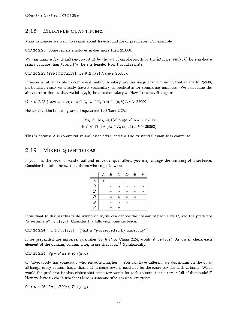
2.19 Mixed quantifiers

If you mix the order of existential and universal quanti�ers, you may change the meaning of a sentence.

Consider the table below that shows who respects who:

A B C D E F

A �B � � � � �C � � � � �D � � � �E � � �F � �

If we want to discuss this table symbolically, we can denote the domain of people by P , and the predicate

\x respects y" by r(x; y). Consider the following open sentence:

Claim 2.24: 9x 2 P; r(x; y) (that is \y is respected by somebody")

If we prepended the universal quanti�er 8y 2 P to Claim 2.24, would it be true? As usual, check each

element of the domain, column-wise, to see that it is.28 Symbolically,

Claim 2.25: 8y 2 P;9x 2 P; r(x; y)

or \Everybody has somebody who respects him/her." You can have di�erent x's depending on the y, so

although every column has a diamond in some row, it need not be the same row for each column. What

would the predicate be that claims that some row works for each column, that a row is full of diamonds?29

Now we have to check whether there is someone who respects everyone:

Claim 2.26: 9x 2 P;8y 2 P; r(x; y)

30

Chapter 2. Logical Notation

You will �nd no such row. The only di�erence between Claim 2.25 and Claim 2.26 is the order of the

quanti�ers. The convention we follow is to read quanti�ers from left to right. The existential quanti�er

involves making a choice, and the choice may vary according to the quanti�ers we have already parsed. As

we move right, we have the opportunity to tailor our choice with an existential quanti�er (but we aren't

obliged to).

Consider this numerical example:

Claim 2.27: 8n 2 N;9m1 2 N;9m2 2 N; n = m1m2.

This says that every natural number has two divisors. What does it mean if you switch the order of the

existentially quanti�ed variables with the universally quanti�ed variable? Is it still true? What (if anything)

would you need to add to say that every natural number has two distinct divisors?30

Chapter 2 Notes

1Yes, by verifying the claim for each employee.

2But contrast the meaning of \di�erentiable functions are continuous" (every di�erentiable function is

continuous, no exception) with the meaning of \birds y" (most birds y, but there are some exceptions).

3Betty makes 5,000, which is well-known to be less than 10,000.

4Restrict to females, and each one make less than 55,000.

5False. Doug and Carlos are counterexamples.

6But it is false for males. Al is a counter-example.

7False, check the table.

8True, check the table.

9Yes, since it includes only elements of itself. Don't confuse subset with proper subset.

10Yes, indeed it is a subset of every set. The reason is that it contains no element that could be outside

another set.

11Claim 2.1 depends on who you mean by \The employee." If you specify Al, Claim 2.1 is false, but if you

specify Ellen, Claim 2.1 is true. Claim 2.2 is quanti�ed, so it depends on the entire universe of employees.

Claim 2.2 is false because you can �nd at least 1 counterexample.

12An untrue implication in the universe we're considering, due to the counter-example Al.

13P (the complement of P ), and Q.

14P (we know it's a subset of Q) and Q (the complement of Q, we know it's a subset of P ).

15Add Grn x to F � L (F outside L). Now Grn x is a counter-example to the claim that every female

employee makes less than 55,000.

16No. Counter-example Grn x makes the implication false, and adding other data doesn't change this.

17Yes. The only Venn diagram that contradicts Claim 2.3 or its contrapositive is one that has at least one

element in F outside of L.

31

Course notes for csc 165 h

18No, because there are elements in L� F (Doug and Carlos).

19We need to verify the following claims:

� If Al is male, then Al makes less than 55,000.

� If Betty is male, then Betty makes less than 55,000.

� If Carlos is male, then Carlos makes less than 55,000.

� If Doug is male, then Doug makes less than 55,000.

� If Ellen is male, then Ellen makes less than 55,000.

� If Flo is male, then Flo makes less than 55,000.

20True, regardless of the cloud situation. In logic P)Q is false exactly when P is true and Q is false. All

other con�gurations of truth values for P and Q are true (assuming that we can evaluate whether P and Q

are true or false).

21All these claims are true, although possibly misleading. Any claim about elements of the empty set is

true, since there are no counterexamples.

22Every employee who makes between 25,000 and 45,000 is male.

239x 2 O; p(x) ^ 9y 2 O; t(y), or even 9x 2 O; 9y 2 O; p(x) ^ t(y).249x 2 O; p(x) ^ t(x)25\P exclusive-or Q" is the same as \P not-equivalent-to Q."

26If you have n predicates, you need 2n rows (every combination of T and F).

27It implies that P is a subset of R, since P � Q and Q � R. It is not equivalent, since you can certainly

have P � R without P � Q or R � Q.

28True, there's a diamond in every column.

29If we were thinking of the row corresponding to x, then 8y 2 P; r(x; y).

308n 2 N; 9m1 2 N; 9m2 2 N; n = m1m2 ^m1 6= m2. Not true for n = 1.

32

Chapter 3

Proofs

3.1 What is a proof?

A proof is an argument that convinces someone who is logical, careful and precise. The form and detail of a

proof can depend on the audience (for example, whether our audience has as much general math knowledge,

and whether we're writing in English or our symbolic form), but the fundamentals are the same whether

we're talking mathematics, computer science, physical sciences, philosophy, or writing an essay in literature

class. A proof communicates what (and how) someone understands, to save others time and e�ort. If you

don't understand why something is true, don't expect to be able to prove it!

How do you go about writing a proof? Generally, there are two steps or phases to creating a proof:

1. Understanding why something is true.

This step typically requires some creativity and multiple attempts until an approach works. You should

ask yourself why you are convinced something is true, and try to express your thoughts precisely and

logically. This step is the most important (and requires the most e�ort), and can be done in the shower

or as you lie awake in bed (the two most productive thinking spots).

Sometimes we call this finding a proof.

2. Writing up your understanding.

Be careful and precise. Every statement you write should be true in the context it's written. It is often

helpful to use our formal symbolic form, to ensure you're careful and precise. Often you will detect

errors in your understanding, and it's common to then go back to step 1 to re�ne your understanding.

This is when we are writing up a proof.

Sometimes these steps can be combined, and often these steps feedback on each other. As we try to write

up our understanding, we discover a aw, return to step 1 and re�ne our understanding, and try writing

again.

Students are often surprised that most of the work coming up with a proof is understanding why some-

thing is true. If you go back to our de�nition of what is a proof, this should be obvious: to convince someone,

we �rst need to convince ourselves and order our thoughts precisely and logically. You will see that once we

gain a good understanding, proofs nearly write themselves.

Taxonomy of results

A lemma is a small result needed to prove something we really care about. A theorem is the main result

that we care about (at the moment). A corollary is an easy (or said to be easy) consequence of another

result. A conjecture is something suspected to be true, but not yet proven.1 An axiom is something we

assert to be true, without justi�cation|usually because it is \self-evident."2

33

Course notes for csc 165 h

3.2 Direct proof of universally-quantified implication

We want to make convincing arguments that a statement is true. We're allowed (forced, actually) to use

previously proven statements and axioms. For example, if D is the set of real numbers, then we have plenty

of rules about arithmetic and inequalities in our toolbox. From these statements, we want to extend what

we know, eventually to include the statement we're trying to prove. Let's examine how we might go about

doing this.

Consider an implication we would like to prove that is of the form:

c1: 8x 2 D; p(x)) q(x)

Many already-known-to-be-true statements are universally quanti�ed implications, having an identical struc-

ture to c1. We'd like to �nd among them a chain:

c2.0: 8x 2 D; p(x)) r1(x)

c2.1: 8x 2 D; r1(x)) r2(x)

...

c2.n: 8x 2 D; rn(x)) q(x)

This, in n steps, proves c1, using the transitivity of implication.

A more exible way to summarize that the chain c2.0,: : : ,c2.n proves c1 is to cite the intermediate

implications that justify each intermediate step. Here you write the proof that 8x 2 D; p(x)) q(x) as:

Assume x 2 D. # x is a generic element of D

Assume p(x). # x has property p, the antecedent

Then r1(x). # by c2.0

Then r2(x). # by c2.1...

Then q(x). # by c2.n

Then p(x)) q(x). # assuming antecedent leads to consequent

Then 8x 2 D; p(x)) q(x). # we only assumed x is a generic D

This form emphasizes what each existing result adds to our understanding. And when it's obvious which

result was used, we can just avoid mentioning it (but be careful, one person's obvious is another's mystery).

Although this form seems to talk about just one particular x, by not assuming anything more than x 2 D

and p(x), it applies to every x 2 D with p(x).

The indentation shows the scope of our assumptions. When we assume that x 2 D, we are in the \world"

where x is a generic element of D. Where we assume p(x), we are in the \world" where p(x) is assumed

true, and we can use that to derive consequences.

Hunting the elusive direct proof

In general, the di�culty with direct proof is there are lots of known results to consider. The fact that a

result is true may not help your particular line of argument (there are many, many, many true but irrelevant

facts). In practice, to �nd a chain from p(x) to q(x), you gather two lists of results about x:

1. results that p(x) implies, and

2. results that imply q(x)

Your fervent hope is that some result appears on both lists, since then you'll have a chain.

34

Chapter 3. Proofs

p(x)

r1(x)

r2(x)

...

s2(x)

s1(x)

q(x)

Anything that one of the ri implies can be added to the �rst list. Anything that implies one of the si can

be added to the second list.

What does this look like in pictures? In Venn diagrams we can think of the ri as sets that contain p and

may, or may not, be contained in q (the ones that aren't contained in q are dead ends). On the other hand,

the si are contained in q and may, or may not, contain p (the ones that don't are dead ends). We hope to

�nd a patch of containment from p to q. Another way to visualize this is by having the ri represented as a

tree. In one tree we have root p, with children being the ri that p implies, and their children being results

they imply. In a second tree we have root q, with children being the results that imply q, and their children

being results that imply them. If the two trees have a common node, we have a chain.

Are you done when you �nd a chain? No, you write it up, tidying as you go. Remove the results that

don't contribute to the �nal chain, and cite the results that take you to each intermediate link in the chain.

What do ^ and _ do?

Now your two lists have the form

8x 2 D; p(x)) (r1(x) ^ r2(x) ^ � � � ^ rm(x))8x 2 D; (sk(x) _ � � � _ s1(x))) q(x)

Since p(x) implies any \and" of the ri, you can just collect them in your head until you �nd a known

result, say r1(x) ^ r2(x)) rk(x), and then add rk(x) to the list. On the other hand, if you have a result

on the �rst list of the form r1(x) ^ r2(x), you can add them separately to the list. On the second list,

use the same approach but substitute _ for ^. Any result on the �rst list can be spuriously \or'ed" with

anything: r1(x)) (r1(x)_ l(x)) is always true. On the second list, we can spuriously \and" anything, since

(s1(x) ^ l(x))) s1(x).

If we have a disjunction r1(x) _ r2(x) on the �rst list, we can use it if we have a result that (r1(x) _r2(x))) q(x), or the pair of results r1(x)) q(x), and r2(x)) q(x).

3.3 An odd example of direct proof

Suppose you are asked to prove that every odd natural number has a square that is odd. Typically we don't

see all the links in the chain from \n is odd" to \n2 is odd" instantly, so we engage in thoughtful wishing

(like wishful thinking, only with a much better reputation). We start by writing the outline of the proof we

would like to have, to clarify what information we've got, what we lack, and hope to �ll in the gaps:

Assume n 2 N.Assume n is odd.

...

Then n2 is odd.

Then n is odd )n2 is odd.

Then 8n 2 N; n is odd )n2 is odd.

35

Course notes for csc 165 h

Start scratching away at both ends of the... (the bit that represents the chain of results we need to �ll in).

What does it mean for n2 to be odd? Well, if there is a natural number k such that n2 = 2k + 1, then n2

is odd (by de�nition of odd numbers). Add that to the end of the list. Similarly, if n is odd, then there is

a natural number j such that n = 2j + 1 (by de�nition of odd numbers). It seem unpromising to take the

square root of 2k+1, so instead carry out the almost-automatic squaring of 2j+1. Now, on our �rst list, we

have that, for some natural number j, n2 = 4j2+4j+1. Using some algebra (distributivity of multiplication

over addition), this means that for some natural number j, n2 = 2(2j2+2j)+1. If we let k from our second

list be 2j2 + 2j, then we certainly satisfy the restriction that k be a natural number (they are closed under

multiplication and addition), and we have linked the �rst list to the second. Here's an example of how to

format your �nished chain:

Assume n 2 N. # n is a generic natural number

Assume n is odd. # n a typical odd natural number

Then, 9j0 2 N, n = 2j0 + 1. # by de�nition of n odd

Let j 2 N be such that n = 2j + 1. # name it j

Then n2 = 4j2 + 4j + 1 = 2(2j2 + 2j) + 1. # de�nition of n2 and some algebra

Then 9k 2 N; n2 = 2k + 1. # 2j2 + 2j 2 N, since N closed under +;�Then n2 is odd. # by de�nition of n2 odd

Then n is odd )n2 is odd. # when I assumed n odd, I derived n2 odd

Then 8n 2 N, n odd ) n2 odd. # since n was a generic natural number

How about the converse, 8n 2 N; if n2 is odd, then n is odd. If we try creating a chain, it seems a bit as

though the natural direction is wrong: somehow we'd like to go from q back to p. What equivalent of an

implication allows us to do this?3 You set up the proof of the contrapositive of the converse (whew!) very

similarly to the proof above, mostly changing \odd" to \even." Try it out.

Another example of direct proof

Let R be the set of real numbers. Prove:

8x 2 R; x > 0) 1=(x+ 2) < 3

Structure the proof as before:

Assume x 2 R. # x is a typical real number

Assume x > 0. # antecedent... # prove 1=(x+ 2) < 3

Then 1=(x+ 2) < 3. # get here somehow

Then x > 0 ) 1=(x+ 2) < 3. # assume antecedent, derived consequent

Then 8x 2 R; x > 0) 1=(x+ 2) < 3. # only assume x was a typical element of R

Of course, you need to unwrap the sub-proof that 1=(x+ 2) < 3:

Assume x 2 R. # x is a typical element of R

Assume x > 0. # antecedent

Then x+ 2 > 2. # x > 0, add 2 to both sides

Then 1=(x+ 2) < 1=2. # reciprocals reverse inequality, and are de�ned for numbers > 2

Then 1=(x+ 2) < 3. # since 1=(x+ 2) < 1=2 and 1=2 < 3

Then x > 0 ) 1=(x+ 2) < 3. # assumed antecedent, derived consequent

Then 8x 2 R; x > 0) 1=(x+ 2) < 3. # x was assumed to be a typical element of R

Is the converse true (what is the converse)?4

36

Chapter 3. Proofs

3.4 Indirect proof of universally-quantified implication

Recall that p) q is equivalent to its contrapositive, :q):p. This means that proving one proves the other.

This is called an \indirect proof." The outline format of an indirect proof of 8x 2 D; p(x)) q(x) is

Assume x 2 D. # x is a typical element of D

Assume :q(x). # negation of the consequent!...

Then :p(x). # negation of the antecedent!

Then :q(x)):p(x). # assuming :q(x) leads to :p(x)Then p(x)) q(x). # implication is equivalent to contrapositive

Then 8x 2 D; p(x)) q(x). # x was a typical element of D

This is a useful approach, for example, in proving that 8n 2 N; n2 is odd )n is odd.

3.5 Direct proof of universally-quantified predicate

When no implication is stated, then we don't assume (suppose) anything about x other than membership

in the domain. For example, 8x 2 D; p(x) has this proof structure:

Assume x 2 D.... # prove p(x)

Then p(x).

Then 8x 2 D; p(x). # x was assumed to be a typical element of D

3.6 Proof by contradiction

Sometimes you want to prove a conclusion, Q, without any suitable hypothesis, P to imply it. One approach

is to say \if everything we already know is true is assumed, then Q follows." How do you choose which

particular portion of \everything we already know is true" to focus on? Let logic help focus your argument.

Symbolically you can represent \everything we already know is true" as a huge conjunction of statements,

P = P1 ^ P2 ^ � � � ^ Pm. So now we aim to prove P ) Q using the contrapositive: :Q) :P . Start

by assuming that Q is false, and then show that something you already know to be true must be false|

a contradiction! Since P = P1 ^ P2 ^ � � � ^ Pm is a huge conjunction of statements, its negation is a huge

disjunction :P = :P1_:P2_� � �_:Pm, so you don't need to know in advance which of them is contradicted.

You just follow your (educated) nose. Here's the general format:

Assume :Q. # in order to derive a contradiction... # some steps leading to a contradiction, say :Pj

Then :P . # contradiction, since P is known to be true

Then Q. # since assuming :Q leads to contradiction

Euclid used this technique over 2,000 years ago to prove that there are in�nitely many prime numbers.

Before looking at Euclid's proof, you might experiment with proving this fact directly.

Let's start by naming some of the sets/predicates we'll need for this proof:

� P = fp 2 N : p has exactly two factorsg� sp: 8n 2 N; jP j > n

In spite of appearances, sp is not a good candidate for mathematical induction (which we'll see later in this

course). However, let's try :sp:

37

Course notes for csc 165 h

Assume :sp: 9n 2 N; jP j 6 n. # to derive a contradiction

Then there is a �nite list, p1; : : : ; pk of elements of P . # at most n elements in the list

Then I can take the product p0 = p1 � � � � � pk. # �nite products are well-de�ned

Then p0 is the product of some natural numbers 2 and greater. # 0; 1 aren't primes, 2; 3 are

Then p0 > 1. # p0 is at least 6

Then p0 + 1 > 2. # add 1 to both sides

Then 9p 2 P; p divides p0 + 1. # every integer > 2 (such as p0 + 1) has a prime divisor

Let p0 2 P be such that p0 divides p0 + 1. # instantiate existential

Then p0 is one of p1; : : : ; pk. # by assumption, the only primes

Then p0 divides p0 + 1� p0 = 1. # a divisor of each term divides di�erence

Then 1 2 P . Contradiction! # 1 is not prime

Then sp. # \assume :sp" leads to a contradiction

3.7 Direct proof structure of the existential

Consider the example 9x 2 R; x3 +2x2 +3x+4 = 2. Since this is the existential, we need only �nd a single

example to show that the statement is true. We structure the proof as follows:

Let x = �1. # choose a particular element that will work

Then x 2 R. # verify that the element is in the domain

Then x3 +2x2 +3x+4 = (�1)3 +2(�1)2 +3(�1) + 4 = �1+ 2� 3+ 4 = 2. # substitute �1 for xThen 9x 2 R; x3 + 2x2 + 3x+ 4 = 2. # we gave an example

The general form for a direct proof of 9x 2 D; p(x) is:

Let x = : : : # choose a particular element of the domain

Then x 2 D. # this may be obvious, otherwise prove it... # prove p(x)

Then p(x). # you've shown that x satis�es p

9x 2 D; p(x). # introduce existential

3.8 Multiple quantifiers, implications, and conjunctions

Consider 8x 2 D;9y 2 D; p(x; y). The corresponding proof structure is:

Assume x 2 D. # typical element of D

Let yx = : : : # choose an element that works...

Then yx 2 D. # verify that y 2 D...

Then p(x; yx). # y satis�es p(x; y)

Then 9y; p(x; y). # introduce existential

Then 8x 2 D;9y 2 D; p(x; y). # introduce universal

Here's a concrete example. Suppose we have a mystery function f , mystery constants a and l, and the

following statement (I have added parentheses to indicate the conventional parsing):

8e 2 R; e > 0) (9d 2 R; d > 0 ^ (8x 2 R; 0 < jx� aj < d) jf(x)� lj < e))

If we want to prove this true, structure the proof as follows: : :5

38

Chapter 3. Proofs

If we want to prove the statement false, we �rst negate it, and then use one of our proof formats (I use

the equivalences :(p) q), (p ^ :q) and :(p ^ q), (p):q)):

9e 2 R; e > 0 ^ 8d 2 R; d > 0)9x 2 R; 0 < jx� aj < d ^ jf(x)� lj > e

Of course, this negation involved several applications of rules we already know, and now its proof may be

written step-by-step. Notice that, in the middle of our proof, we had a \^" to prove.

3.9 Example of proving a statement about a sequence

Consider the statement:

Claim 3.1: 9i 2 N; 8j 2 N; aj 6 i) j < i

and the sequence:

(A1) 0; 1; 4; 9; 16; 25; : : :

We'll use the convention that sequences are indexed by natural numbers (recall that N = f0; 1; 2; : : : g,starting at zero just as computers count) and ai is the element of the sequence indexed by i, so a0 = 0,

a1 = 1, a2 = 4. Looking at the pattern of (A1), we can write a \closed form" formula for ai.6

We should of course try to understand 3.1, by putting it in natural English, picturing tables and diagrams,

thinking of code that could check it, trying it on various examples, etc. To understand whether it is true

or false for (A1) we should use this understanding, including tracing it. But let's focus on the form that a

proof that 3.1 is true could take. This may even help us understand 3.1.

We have been justifying existentials with an example. So, our proof should start o� something like:

Let i = . Then i 2 N....

We leave ourselves a blank to �ll in: a speci�c value of i. We also need to make sure the i is in N. Often it

will be obvious and we will simply note it. If not, we'll actually need to put in a proof.

Next, we need to prove something for all j in N. As a syntactic convenience, we prove something for all

j's in N by proving it for some unknown j in N. If we're careful to not assume anything about which j we

have, our proof will handle all j's.

Let i = . Then i 2 N. # choose a helpful one

Assume j 2 N. # j is a typical element of N...

Notice this time we assume j is in N. You can imagine 9 and 8 as part of a game:

� 9x 2 D: We get to pick x, but have to follow the rules and pick from D.

� 8x 2 D: Our opponent will pick x, but we can assume they will follow the rules and pick from D. We

can't make any assumptions here about which one from D they will pick.

Going back to our proof structure, we have:

Let i = . Then i 2 N.Assume j 2 N. # typical element of N

Assume aj 6 i....

Then j < i.

39

Course notes for csc 165 h

We leave ourselves room (the...) for a proof of j < i. Once we �ll in a value of i, the proof of j < i may use

three facts: the value we chose for i, j 2 N, and aj 6 i.

After a little thought, we decide that setting i = 2 is a good idea, since then aj 6 i is only true for j = 0

and j = 1, and these are smaller than 2. A bit of experimentation shows that the contrapositive, :(j < i)

) :(aj 6 ai) is a bit easier to work with.

Let i = 2. Then i 2 N. # 2 2 NAssume j 2 N. # typical element of N

Assume :(j < i). # antecedent for contrapositive

Then j > 2. # negation of j < i when i = 2

Then aj = j2 > 22 = 4. # since aj = j2, and j > 2

Then aj > 2. # since 4 > 2

Then :(j < i)):(aj 6 2). # assuming antecedent leads to consequent

Then aj 6 2) j < i. # implication equivalent to contrapositive

Then 8j 2 N; aj 6 i) j < i. # introduce universal

Then 9i 2 N; 8j 2 N; aj 6 i) j < i. # introduce existential

3.10 Example of disproving a statement about a sequence

Consider now the statement:

Claim 3.2: 9i 2 N; 8j 2 N; j > i) aj = ai

and the sequence:

(A2) 0; 0; 1; 1; 2; 2; 3; 3; 4; 4; 5; 5; 6; : : :

Let's disprove it. Is disproof a whole new topic? Thankfully no. We simply prove the negation:

Claim 3.20: 8i 2 N; 9j 2 N; j > i ^ aj 6= ai

As usual, we sketch in the outline of the proof �rst:

Assume i 2 N.Let j = . Then j 2 N....

Then j > i ^ aj 6= ai.

Then 9j 2 N; j > i ^ aj 6= ai. # introduction of existential

Then 8i 2 N; 9j 2 N; j > i ^ aj 6= ai. # introduction of universal

Our opponent picks i, but we get to pick j. And we are allowed to make j depend on i. Unfortunately,

while writing up the proof we can't wait for someone to actually pick i. So how does it help us? We get

to describe a general strategy for how we would pick a particular j if we knew which particular i. In other

words, j can be described as function of i.

In programming terms, i is in scope when we pick j: it has been declared and can be seen from where

we declare j. Notice that j is not in scope when we declare i: so when we picked i for 3.1, we weren't

allowed to use j. If we write a program that uses a variable before it's declared and initialized, the program

doesn't even compile. This is a major error. If you write a proof that does this, it will almost certainly be

wrong|and you will most likely lose a lot of marks!

Now we are left with proving j > i ^ aj 6= ai (notice we wrote this at the bottom. . . we must have been

thinking ahead). What form does the proof of a conjunction take?7

40

Chapter 3. Proofs

Assume i 2 N.Let j = . Then j 2 N....

Then j > i....

Then aj 6= ai.

Then j > i ^ aj 6= ai.

Then 9j 2 N; j > i ^ aj 6= ai.

Then 8i 2 N; 9j 2 N; j > i ^ aj 6= ai.

To �nish this o�, we need to choose a value for j. If we choose wisely, the rest of the proof falls into place.8

What elementary property of arithmetic will we require?9

3.11 Non-boolean function example

Non-boolean functions cannot take the place of predicates (since predicates are expected to return a true or

false value) in a proof. How should non-boolean functions be used? De�ne bxc : R! R by:

bxc (\ oor of x") is the largest integer 6 x.

Now we can form the statement:

Claim 3.3: 8x 2 R; bxc < x+ 1

It makes sense to apply bxc to elements of our domain, or variables that we have introduced, and to evaluate

it in predicates such as \<" but bxc itself is not a variable, nor a sentence, nor a predicate. We can't

(sensibly) say things such as 8bxc 2 R or 8x 2 R; bxc _ bx+ 1c. The structure of 3.3 is a direct proof of a

universally-quanti�ed predicate:10

Assume x 2 R. # x is a typical element of R

Let y = bxc. # introduce a variable

Then y is the largest integer 6 x, so y 6 x. # de�nition of oor

Since x < x+ 1, y < x+ 1. # transitivity of <

So bxc < x+ 1. # since y = bxcThen 8x 2 R; bxc < x+ 1. # since x was a typical element of R

In some cases you need to break down a statement such as \y is the largest integer 6 x":

y 2 Z ^ y 6 x ^ (8z 2 Z; z 6 x) z 6 y)

We didn't need all three parts of the de�nition for our proof above, and in practice we don't always have to

return to de�nitions when dealing with functions. For example, we may have an existing result, such as:

8x 2 R; bxc > x� 1

How would you prove this result, using the three-part version of the de�nition of bxc?

3.12 Substituting known results

Every proof would become unmanageably long if we had to include \inline" all the results that it depended

on. We inevitably refer to standard results that are either universally known (among math wonks) or can

easily be looked up. Sometimes we need to prove a small technical result in order to prove something larger.

You may view the smaller result as a helper method (usually returning boolean results) that you use to

build a larger method (your bigger proof). To make things modular, you should be able to \call" or refer to

the smaller result. An example occurs if we want to re-cycle something proved earlier:

41

Course notes for csc 165 h

Theorem 1: 8x 2 R; x > 0) 1=(x+ 2) < 3.

We want to use this in proving 8y 2 R; y 6= 0) 1=(y2 + 2) < 3. The template to �ll in is

Assume y 2 R.Assume y 6= 0.

...

Then 1=(y2 + 2) < 3.

Then y 6= 0) 1=(y2 + 2) < 3.

Then 8y 2 R; y 6= 0) 1=(y2 + 2) < 3.

Now we have to �ll in the... part:

Assume y 2 R. # y is a typical element of R

Assume y 6= 0. # y positive

Then y2 2 R and y2 > 0. # R closed under �, squares of non-zero realsThen y2 > 0, since y2 6= 0 and y2 > 0. # only real number whose square is 0 is 0

Then 1=(y2 + 2) < 3. # by Theorem 1

Then y 6= 0) 1=(y2 + 2) < 3. # introduction of )Then 8y 2 R; y 6= 0) 1=(y2 + 2) < 3. # introduction of universal

3.13 Proof by cases

To prove A)B, it can help to treat some A's di�erently than others. For example, to prove that x2 + x is

even for all integers x, you might proceed by noting that x2 + x is equivalent to x(x+ 1). At this point our

reasoning has to branch: at least one of the factors x or x + 1 is even (for integer x), but we can't assume

that a particular factor is even for every integer x. So we use proof by cases.11

This is a special case of an \or" clause being the antecedent of an implication, i.e., if you want to prove

(A1 _ A2 _ � � � _ An)) B. This could happen if, along the way to proving A) B you use the fact that

A) (A1 _ � � � _ An). Now you need to prove A1 ) B, A2 ) B; : : : ; An ) B. Notice that in setting this up

it is not necessary that the Ai be disjoint (mutually exclusive), just that they cover A (think of A being a

subset of the union of the Ai). One way to generate the cases is to break up the domain D = D1 [ � � � [Dn,

so Ai is the predicate that corresponds to the set Di \A. Now you have an equivalence, A,A1 _ � � � _An.

A very common case occurs when the domain partitions into two parts, D = D1 [D1, so you can rewrite A

as (A ^D1) _ (A ^ :D1)|we're abusing the notation slightly here by treating D1 both as a set and as a

predicate, as we've done before.

Here's the general form of proving something by cases:

A _BCase 1: Assume A.

...

Then C.

Case 2: Assume B....

Then C.

Since A _B and in both (all) cases we concluded C, then C.

Remember that we need one case for each disjunct, so if we knew A1 _ � � � _ An, we'd need n cases.

When you're reading (or writing) proofs, often the word \assume" is omitted when de�ning the case.

Though it might say \Case x < k," remember that x < k is an assumption, thus opens a new indentation

(scope) level.

42

Chapter 3. Proofs

Law of the excluded middle

Often we want to proceed by cases, but don't have a disjunction handy to use. We can always introduce

one using the Law of the Excluded Middle. This law of logic states that a formula is either true or

false|there's nothing between (or \in the middle"). Thus, for any formula P , the following is sure to be

true:

P _ :PIn your proof, you can then split into two cases depending on whether P is true or false. Just be sure to

negate P correctly!

Example proof using cases

Suppose we wanted to prove the following statement: if n is an integer then n2 + n is even.

Let's formalize what we mean by the term \integer n is even":

For n 2 Z, let even(n) mean 9k 2 Z; n = 2k.

Let's formalize what we're proving:

Claim 3.4: 8n 2 Z; 9k 2 Z; n2 + n = 2k.

Noticing that n2+n = n(n+1), we consider whether n is odd or even. We know that every integer is either

odd or even, so let's state this formally:

(*) 8n 2 Z; (9k 2 Z; n = 2k + 1) _ (9k 2 Z; n = 2k).

Now to the proof of our claim. In it we will know that an existential is true, and we will want to use that

knowledge. We may ask the existential to \return" an example element, which we get to name and use (we

name it k0 so that it won't con ict with any other elements we're talking about).

Assume n 2 Z. # n is a typical natural number

Then (9k 2 Z; n = 2k + 1) _ (9k 2 Z; n = 2k). # by (*), n 2 ZCase 1: Assume 9k 2 Z; n = 2k + 1.

Let k0 2 Z be such that n = 2k0 + 1. # instantiate existential

Then n2 + n = n(n+ 1) = (2k0 + 1)(2k0 + 2) = 2(2k0 + 1)(k0 + 1).

Then 9k 2 Z; n2 + n = 2k. # k = (2k0 + 1)(k0 + 1) 2 ZCase 2: Assume 9k 2 Z; n = 2k.

Let k0 2 Z be such that n = 2k0. # instantiate existential

Then n2 + n = n(n+ 1) = 2k0(2k0 + 1) = 2[k0(2k0 + 1)].

Then 9k 2 Z; n2 + n = 2k. # k = k0(2k0 + 1) 2 ZThen 9k 2 Z; n2 + n = 2k. # true in all (both) possible cases

Then 8n 2 Z; 9k 2 Z; n2 + n = 2k. # introduction of universal

Proving _ using cases

Let's prove that the square of an integer is a triple or one more than a triple.

Claim 3.5: 8n 2 N; (9k 2 N; n2 = 3k) _ (9k 2 N; n2 = 3k + 1).

If we know P _Q, we can prove a disjunction R _ S by cases, as follows:

P _QCase 1: Assume P .

...

Then R.

43

Course notes for csc 165 h

Case 2: Assume Q....

Then S.

Thus R _ S.12

If we already have some P _Q we can use, then those are the obvious cases to consider, though we still have

to decide between the two ways of pairing them up with R and S. In general though, picking P and Q that

work depends completely on context. When constructing proof structures, a standard strategy is to use :Pfor Q: the Law of the Excluded Middle ensures this is true, and it is the simplest yet still general structure.

This of course generalizes to more than two cases: if we know P1 _ P2 _ � � � _ Pn, and we want to prove

Q1 _ � � � _Qm, then we can do cases for each Pi, in each case proving a Qj . We don't have to prove all the

Qj , and we can prove some of them in more than one case.

To prove our claim, we want to use part of the Remainder Theorem:

(*) 8n 2 N; (9k 2 N; n = 3k _ n = 3k + 1 _ n = 3k + 2)

We now proceed with our proof of the claim by cases. One case is left for you to do as an exercise.

Assume n 2 N. # n is a typical element of N

Then 9k 2 N; n = 3k _ n = 3k + 1 _ n = 3k + 2. # by (*)

Let k0 2 N be such that n = 3k0 _ n = 3k0 + 1 _ n = 3k0 + 2.

Case 1: Assume n = 3k0.

Then 3(3k20) = 9k20 = n2. # algebra

Then 9k 2 N; n2 = 3k. # k = 3k20 2 NCase 2: Assume n = 3k0 + 1.

Then 3(3k20 + 2k0) + 1 = 9k20 + 6k + 1 = n2. # algebra

Then 9k 2 N; n2 = 3k + 1. # k = 3k20 + 2k0 2 NCase 3: Assume n = 3k0 + 2.

(Exercise.)

Then (9k 2 N; n2 = 3k) _ (9k 2 N; n2 = 3k + 1). # true in all possible cases

Then 8n 2 N; (9k 2 N; n2 = 3k) _ (9k 2 N; n2 = 3k + 1). # introduction of universal

3.14 Building formulae and taking formulae apart

So far we've been concentrating on proving more and more complicated sentences. This makes sense, since

the sentence we've proving determines the structure our proof will take. For each of the logical connectives

and quanti�ers, we've seen structures that allow us to conclude big statements from smaller ones. The

inference rules that allow us to do this are collectively called introduction rules, since they allow us to

introduce new sentences of a particular type.

But rarely do we prove things directly from predicates. We often have to use known theorems and results

or separately proven lemmas to reduce the length of our proofs to a manageable size (can you imagine always

having to prove 2 + 2 = 4 from primitive sets each time you use this fact?). Good theorems are useful in

a number of settings, and typically use a number of connectives and quanti�ers. Knowing how to break

complex sentences down is equally important as knowing how to build complex sentences up.

Just as there are inference rules allowing us to introduce new, complex sentences, there are inference rules

allowing us to break sentences down in a formal, precise and valid way. These rules are collectively called

elimination rules, since they allow us to eliminate connectives and quanti�ers we don't want anymore.

Most rules should be fairly straight-forward and should make sense to you at this point; if not, you should

review your manipulation rules.

44

Chapter 3. Proofs

Double negation elimination

We can't do much to remove one negation (unless we can move it further inside), but we know how to get

rid of two negations. Indeed, this was a manipulation rule from the previous chapter, but we can also treat

it as a reasoning rule: if we know ::A is true, we know A is true.

Conjunction elimination

Nearly as easy as negation, how can we break up a conjunction? If we know A^B, what can we conclude?13

Existential elimination (or instantiation)

We might know that 9x 2 D;B, where B likely mentions x somewhere inside. In other words, we know B

is true for some element in D, but we don't know which one. How can we proceed? We'd probably like to

say something about that element in D that B is true for, but how do we know which element it is?

We don't really need to know which element B is true for, only that it exists. We can proceed by using

B with every reference to x replaced by a new variable x0 (just notation to distinguish it from x).

Disjunction elimination

A _ B itself cannot be split, as we don't know which part of the disjunction is true. However, if we also

know :A, we can conclude B must be true. Analogously, with :B we can conclude A.

Another good way to deal with a disjunction is proof by cases, which we discussed above.

Implication elimination

Suppose we know A)B. If we are able to show A is true, then we could immediately conclude B. This is

perhaps the most basic reasoning structure, and has a fancy latin name: modus ponens (meaning \mode

that a�rms"). This form is the basis to deductive argument (you can imagine Sherlock Holmes using modus

ponens to reveal the criminal).

On the other hand, if we knew :B, we could still get something from A)B: we'd be able to conclude

:A. This form of reasoning is using the contrapositive and is known as modus tollens (Latin for \mode

that denies").

We can also appeal to the manipulation rules to rewrite A) B as a disjunction, :A _ B, and expand

this formula as desired.

Bi-implication elimination

To take apart a sentence like A,B, we simply exploit its equivalence to (A)B)^ (B)A) and expand it

appropriately.

If we also know A, we can skip some work and directly conclude that B must be true (using the implication

A) B hidden in the bi-implication). Likewise, if we also knew :A, we could conclude :B. Each of these

properties are easily proven using preceding rules.

Universal elimination (or instantiation)

Suppose you know that 8x 2 D;B(x). How can we use this fact to help prove other things? This sentence

says B(x) is true for all members of domain D. So we could use this as meaning a huge conjunction over all

the elements of D = fd1; d2; d3; : : : g:

B(d1) ^B(d2) ^B(d3) ^ : : :

45

Course notes for csc 165 h

>From this expansion (even if we can't write it14) it's clear that if a 2 D, we can conclude that B(a) is true.

This is sometimes called universal instantiation, or universal specialization, since we're allowed to conclude

a specialized statement from our general statement. Intuitively, what holds for everything must hold for any

speci�c thing. Typically, a will have been mentioned already, and you'll want to express that a has some

speci�c property (in this case, B(a)).

3.15 Summary of inference rules

There are several basic and derived rules we're allowed to use in our proofs. Most of them are summarized

below. For each rule, if you know (have already shown) everything that is above the line, you are allowed

to conclude anything that's below the line.

Introduction rules

[:I] negation introduction

Assume A...

contradiction

:A[^I] conjunction introduction

A

B

A ^B[_I] disjunction introduction

A

A _BB _ A

A _ :A

[)I] implication introduction

(direct)

Assume A...

B

A)B

(indirect)

Assume :B...

:AA)B

[,I] equivalence/bi-implication

introduction

A)B

B) A

A,B

[8I] universal introductionAssume a 2 D...

P (a)

8x 2 D;P (x)

[9I] existential introductionP (a)

a 2 D

9x 2 D;P (x)

Elimination rules

[:E] negation elimination

::AA

A

:Acontradiction

[^E] conjunction elimination

A ^BA

B

[_E] disjunction elimination

A _B:AB

A _B:BA

[)E] implication elimination

(Modus

Ponens)

A)B

A

B

(Modus

Tollens)

A)B

:B:A

[,E] equivalence/bi-implication

elimination

A,B

A)B

B) A

[8E] universal elimination

8x 2 D;P (x)

a 2 D

P (a)

[9E] existential elimination

9x 2 D;P (x)

Let a 2 D such that P (a)...

It may surprise you to learn that by this point, we've covered all of the basic proof techniques you will need

during your undergraduate career (and beyond). There is one basic proof technique that we have yet to

46

Chapter 3. Proofs

cover (mathematical induction) but it is more properly the main subject of the course csc 236 h. (Though

we will discuss it a little bit in the next chapter.)

Given this, you may feel that the proofs we've worked on so far have been nowhere near as complicated

as what you might �nd in your calculus textbook, for example. But if you take the time to examine the

structure of any such proof, you will most likely �nd that all of the techniques it uses were covered in this

chapter. The complexity of these proofs stem, not from using more complex techniques, but from their scale

and their reliance on numerous other results and complex de�nitions.

This is no di�erent from the contrast between small programs and large ones: both are written using

the same programming language, which provides just a small set of \building blocks"|conditionals, loops,

functions, etc. The complexity of larger programs stems mainly from their size and/or their reliance on

numerous external libraries.

Bearing this in mind, you now have all of the tools required to understand and appreciate some of the

deepest and most beautiful results in the theory of computation (see Chapter 5). But �rst, in the next

chapter, we'll apply those tools to something more concrete: the analysis of algorithms.

Chapter 3 Notes

1Here's an example of a conjecture whose proof has evaded the best minds for almost 75 years|maybe

you'll prove it? De�ne f(n), for n 2 N, as follows:

f(n) =

(n=2; n even;

3n+ 1; n odd:

Then de�ne fk+1(n) as f(fk(n)), for all k 2 N, with special case f0(n) = n. (So f1(n) = f(n), f2(n) =

f(f(n)), etc.)

Conjecture: 8n 2 N; n > 1)9k 2 N; fk(n) = 1.

Easy to state, but (so far) hard to prove or disprove.

2For example, \for any two points on the plane, there is exactly one line that passes through both points"

is an axiom in Euclidian geometry.

3The contrapositive.

48x 2 R; 1=(x+2) < 3)x > 0. False, for example let x = �4, then 1=(�4+2) = �1=2 < 3 but �4 6> 0.

Indeed, every x < �2 is a counter-example.

5 Assume e 2 R. # typical element of R

Assume e > 0. # antecedent

Let de = : : : # something helpful, probably depending on e

Then de 2 R. # verify de is in the domain

Then de > 0. # show de is positive

Assume x 2 R. # typical element of R

Assume 0 < jx� aj < de. # antecedent...

Then jf(x)� lj < e. # inner consequent

Then 0 < jx� aj < de ) (jf(x)� lj < e). # introduce implication

Then 8x 2 R; 0 < jx� aj < de ) (jf(x)� lj < e). # introduce universal

Then 9d 2 R; d > 0 ^ (8x 2 R; 0 < jx� aj < d) (jf(x)� lj < e)). # introduce existential

Then, e > 0) (9d 2 R; d > 0 ^ (8x 2 R; 0 < jx� aj < d) (jf(x)� lj < e))).

Then 8e 2 R; e > 0) (9d 2 R; d > 0 ^ (8x 2 R; 0 < jx� aj < d) (jf(x)� lj < e))).

47

Course notes for csc 165 h

6In other words, a formula that depends only on i. In this case, we see that ai = i2.

7We need to prove both pieces of a conjunction.

8Try j = i+ 2.

98a 2 N; 8b 2 N; b > 0) a+ b > a.

10 Assume x 2 R....

Then bxc < x+ 1.

Then 8x 2 R; bxc < x+ 1.

11 Assume x 2 Z. # x is a typical integer

Either x is even or x is odd.

Case 1: [Assume] x is even.

Then x(x+ 1) is even. # if x is a multiple of 2, so is x(x+ 1)

Case 2: [Assume] x is odd.

Then x+ 1 is even. # if x leaves remainder 1, x+ 1 leaves remainder 0

Then x(x+ 1) is even. # if x+ 1 is a multiple of 2, so is x(x+ 1)

Then x(x+ 1) is even. # true in all (both) possible cases

Then 8x 2 Z; x(x+ 1) is even. # introduce universal

12Instead of concluding R in one case and S in the other, we are actually concluding R _ S in both cases,

and then we bring R _ S outside the cases because we concluded it in each case, and one of the cases must

hold. (Remember that once we conclude that R is true, we can immediately conclude that R _ S is true.)

So this is exactly the same structure we've seen before.

13We know that A is true and that B is true.

14All our sentences are �nite in length, so if our domain D is in�nite (like the natural numbers or real

numbers), we can't actually write this expansion down. That's the reason why we need a universal quanti�er

in our logic system.

48

Chapter 4

Algorithm Analysis and Asymptotic

Notation

4.1 Correctness, running time of programs

So far we have been proving statements about databases, mathematics and arithmetic, or sequences of

numbers. Though these types of statements are common in computer science, you'll probably encounter

algorithms most of the time. Often we want to reason about algorithms and even prove things about them.

Wouldn't it be nice to be able to prove that your program is correct? Especially if you're programming a

heart monitor or a NASA spacecraft?

In this chapter we'll introduce a number of tools for dealing with computer algorithms, formalizing their

expression, and techniques for analyzing properties of algorithms, so that we can prove correctness or prove

bounds on the resources that are required.

4.2 Binary (base 2) notation

Let's �rst think about numbers. In our everyday life, we write numbers in decimal (base 10) notation

(although I heard of one kid who learned to use the �ngers of her left hand to count from 0 to 31 in base

2). In decimal, the sequence of digits 20395 represents (parsing from the right):

5 + 9(10) + 3(100) + 0(1000) + 2(10000) =

5(100) + 9(101) + 3(102) + 0(103) + 2(104)

Each position represents a power of 10, and 10 is called the base. Each position has a digit from [0; 9]

representing how many of that power to add. Why do we use 10? Perhaps due to having 10 �ngers

(however, humans at various times have used base 60, base 20, and mixed base 20,18 (Mayans)). In the last

case there were (105)20;18 days in the year. Any integer with absolute value greater than 1 will work (so

experiment with base �2).Consider using 2 as the base for our notation. What digits should we use?1 We don't need digits 2 or

higher, since they are expressed by choosing a di�erent position for our digits (just as in base 10, where

there is no single digit for numbers 10 and greater).

Here are some examples of binary numbers:

(10011)2

represents

1(20) + 1(21) + 0(22) + 0(23) + 1(24) = (19)10

49

Course notes for csc 165 h

We can extend the idea, and imitate the decimal point (with a \binary point"?) from base 10:

(1011:101)2 = 195

8

How did we do that?2 Here are some questions:

� How do you multiply two base 10 numbers?3 Work out 37� 43.

� How do you multiply two binary numbers?4

� What does \right shifting" (eliminating the right-most digit) do in base 10?5

� What does \right shifting" do in binary?6

� What does the rightmost digit tell us in base 10? In binary?

Convert some numbers from decimal to binary notation. Try 57. We'd like to represent 57 by adding either

0 or 1 of each power of 2 that is no greater than 57. So 57 = 32 + 16 + 8 + 1 = (111001)2. We can also �ll

in the binary digits, systematically, from the bottom up, using the % operator from Python (the remainder

after division operator, at least for positive arguments):

57 % 2 = 1 so (?????1)2

(57� 1)=2 = 28 % 2 = 0 so (????01)2

28=2 = 14 % 2 = 0 so (???001)2

14=2 = 7 % 2 = 1 so (??1001)2

(7� 1)=2 = 3 % 2 = 1 so (?11001)2

(3� 1)=2 = 1 % 2 = 1 so (111001)2

Addition in binary is the same as (only di�erent from. . . ) addition in decimal. Just remember that (1)2 +

(1)2 = (10)2. If we add two binary numbers, this tells us when to \carry" 1:

1011

+ 1011

10110

log2

How many 5-digit binary numbers are there (including those with leading 0s)? These numbers run from

(00000)2 through (11111)2, or 0 through 31 in decimal|32 numbers. Another way to count them is to

consider that there are two choices for each digit, hence 25 strings of digits. If we add one more digit we get

twice as many numbers. Every digit doubles the range of numbers, so there are two 1-digit binary numbers

(0 and 1), four 2-digit binary numbers (0 through 3), 8 3-digit binary numbers (0 through 7), and so on.

Reverse the question: how many digits are required to represent a given number. In other words, what

is the smallest integer power of 2 needed to exceed a given number? log2 x is the power of 2 that gives

2log2 x = x. You can think of it as how many times you must multiply 1 by 2 to get x, or roughly the number

of digits in the binary representation of x. (The precise number of digits needed is dlog2(x+ 1)e|which

happens to be equal to b(log2 x) + 1c for all positive values of x).

4.3 Loop invariant for base 2 multiplication

Integers are naturally represented on a computer in binary, since a gate can be in either an on or o� (1 or

0) position. It is very easy to multiply or divide by 2, since all we need to do is perform a left or right shift

(an easy hardware operation). Similarly, it is also very easy to determine whether an integer is even or odd.

Putting these together, we can write a multiplication algorithm that uses these fast operations:

50

Chapter 4. Algorithm Analysis and Asymptotic Notation

def mult(m,n):

""" Multiply integers m and n. """

# Precondition: m >= 0

x = m

y = n

z = 0

# loop invariant: z = mn - xy

while x != 0:

if x % 2 == 1: z = z + y # x is odd

x = x >> 1 # x = x / 2 (right shift)

y = y << 1 # y = y * 2 (left shift)

# post condition: z = mn

return z

After reading this algorithm, there is no reason you should believe it actually multiplies two integers: we'll

need to prove it to you. Let's consider the precondition �rst. So long as m is a positive natural number, and

n is an integer, the program claims to work. The postcondition states that z, the value that is returned, is

equal to the product of m and n (that would be nice, but we're not convinced).

Let's look at the stated loop invariant. A loop invariant is a relationship between the variables that is

always true at the start and at the end of a loop iteration (we'll need to prove this). It's su�cient to verify

that the invariant is true at the start of the �rst iteration, and verify that if the invariant is true at the start

of any iteration, it must be true at the end of the iteration. Before we start the loop, we set x = m, y = n

and z = 0, so it is clear that z = mn � xy = mn �mn = 0. Now we need to show that if z = mn � xy

before executing the body of the loop, and x 6= 0, then after executing the loop body, z = mn� xy is still

true (can you write this statement formally?). Here's a sketch of a proof:

Assume xi; yi; zi; xi+1; yi+1; zi+1;m; n 2 Z, where xi represents the value of variable x at the beginningof the ith iteration of the loop, and similarly for the other variables and subscripts. (Note that there

is no need to subscript m;n, since they aren't changed by the loop.)

Assume zi = mn� xiyi.

Case 1: Assume xi odd.

Then zi+1 = zi + yi, xi+1 = (xi � 1)=2, and yi+1 = 2yi.

So mn� xi+1yi+1 = mn� (xi � 1)=2 � 2yi (since xi is odd)

= mn� xiyi + yi

= zi + yi

= zi+1:Case 2: Assume xi even.

Then zi+1 = zi, xi+1 = xi=2, and yi+1 = 2yi.

So mn� xi+1yi+1 = mn� xi=2 � 2yi= mn� xiyi

= zi

= zi+1:Since xi is either even or odd, in all cases mn� xi+1yi+1 = zi+1

Thus mn� xiyi = zi )mn� xi+1yi+1 = zi+1.

Since xi; xi+1; yi; yi+1; zi; zi+1;m; n are arbitrary elements,

8xi; xi+1; yi; yi+1; zi; zi+1;m; n 2 Z;mn� xiyi = zi )mn� xi+1yi+1 = zi+1.

We should probably verify the postcondition to fully convince ourselves of the correctness of this algorithm.

We've shown the loop invariant holds, so let's see what we can conclude when the loop terminates (i.e.,

51

Course notes for csc 165 h

when x = 0). By the loop invariant, z = mn � xy = mn � 0 = mn, so we know we must get the right

answer (assuming the loop eventually terminates).

We should now be fairly convinced that this algorithm is in fact correct. One might now wonder, how

many iterations of the loop are completed before the answer is returned?

Also, why is it necessary for m > 0? What happens if it isn't?

4.4 Running time of programs

For any program P and any input x, let tP (x) denote the number of \steps" P takes on input x. We need to

specify what we mean by a \step." A \step" typically corresponds to machine instructions being executed,

or some indication of time or resources expended.

Consider the following (somewhat arbitrary) accounting for common program steps:

method call: 1 step + steps to evaluate each argument + steps to execute the method.

return statement: 1 step + steps to evaluate return value.

if statement: 1 step + steps to evaluate condition.

assignment statement: 1 step + steps to evaluate each side.

arithmetic, comparison, boolean operators: 1 step + steps to evaluate each operand.

array access: 1 step + steps to evaluate index.

member access: 2 steps.

constant, variable evaluation: 1 step.

Notice that none of these \steps" (except for method calls) depend on the size of the input (sometimes

denoted with the symbol n). The smallest and largest steps above di�er from each other by a constant of

about 5, so we can make the additional simplifying assumption that they all have the same cost|1.

4.5 Linear search

Let's use linear search as an example.

def LS(A,x):

""" Return an index i such that x == L[i]. Otherwise, return -1. """

i = 0 # (line 1)

while i < len(A): # (line 2)

if A[i] == x: # (line 3)

return i # (line 4)

i = i + 1 # (line 5)

return -1 # (line 6)

Let's trace a function call, LS([2,4,6,8],4):

Line 1: 1 step (i=0)

Line 2: 1 step (0 < 4)

Line 3: 1 step (A[0] == 4)

Line 5: 1 step (i = 1)

52

Chapter 4. Algorithm Analysis and Asymptotic Notation

Line 2: 1 step (1 < 4)

Line 3: 1 step (A[1] == 4)

Line 4: 1 (return 1)

So tLS([2; 4; 6; 8]; 4) = 7. Notice that if the �rst index where x is found is j, then tLS(A; x) will count lines

2, 3, and 5 once for each index from 0 to j � 1 (j indices), and then count lines 2, 3, 4 for index j, and so

tLS(A; x) will be 1 + 3j + 3.

If x does not appear in A, then tLS(A; x) = 1+3 len(A)+ 2, because line 1 executes once, lines 2, 3, and

5 executes once for each index from 0 to len(A)� 1, and then lines 2 and 6 execute.

We want a measure that depends on the size of the input, not the particular input. There are three

standard ways. Let P be a program, and let I be the set of all inputs for P . Then:

Average-case complexity: the weighted average over all possible inputs of size n.

In general

AP (n) =X

x of size n

tP (x) � p(x)

where p(x) is the probability that input x is encountered.

Assuming all the inputs are equally likely, this \simpli�es" to

AP (n) =

Px of size n tP (x)

number of inputs of size n

(Di�cult to compute.)

Best-case complexity: min(tP (x)), where x is an input of size n.

In other words, BP (n) = minftP (x) j x 2 I ^ size(x) = ng.(Mostly useless.)

Worst-case complexity: max(tP (x)), where x is an input of size n.

In other words, WP (n) = maxftP (x) j x 2 I ^ size(x) = ng.(Relatively easy to compute, and gives a performance guarantee.)

What is meant by \input size"? This depends on the algorithm. For linear search, the number of elements

in the array is a reasonable parameter. Technically (in csc 463 h, for example), the size is the number of

bits required to represent the input in binary. In practice we use the number of elements of input (length of

array, number of nodes in a tree, etc.)

4.6 Run time and constant factors

When calculating the running time of a program, we may know how many basic \steps" it takes as a function

of input size, but we may not know how long each step takes on a particular computer. We would like to

estimate the overall running time of an algorithm while ignoring constant factors (like how fast the CPU

is). So, for example, if we have 3 machines, where operations take 3�s, 8�s and 0.5�s, the three functions

measuring the amount of time required, t(n) = 3n2, t(n) = 8n2, and t(n) = n2=2 are considered the same,

ignoring (\to within") constant factors (the time required always grows according to a quadratic function

in terms of the size of the input n).

To view this another way, think back to the linear search example in the previous section. The worst-case

running time for that algorithm was given by the function

W (n) = 3n+ 3

53

Course notes for csc 165 h

But what exactly does the constant \3" in front of the \n" represent? Or the additive \+3"? Neither value

corresponds to any intrinsic property of the algorithm itself; rather, the values are consequences of some

arbitrary choices on our part, namely, how many \steps" to count for certain Python statements. Someone

counting di�erently (e.g., counting more than 1 step for statements that access list elements by index) would

arrive at a di�erent expression for the worst-case running time. Would their answer be \more" or \less"

correct than ours? Neither: both answers are just as imprecise as one another! This is why we want to come

up with a tool that allows us to work with functions while ignoring constant multipliers.

The nice thing is that this means that lower order terms can be ignored as well! So f(n) = 3n2 and

g(n) = 3n2 + 2 are considered \the same," as are h(n) = 3n2 + 2n and j(n) = 5n2. Notice that

8n 2 N; n > 1) f(n) 6 g(n) 6 h(n) 6 j(n)

but there's always a constant factor that can reverse any of these inequalities.

Really what we want to measure is the growth rate of functions (and in computer science, the growth

rate of functions that bound the running time of algorithms). You might be familiar with binary search and

linear search (two algorithms for searching for a value in a sorted array). Suppose one computer runs binary

search and one computer runs linear search. Which computer will give an answer �rst, assuming the two

computers run at roughly the same CPU speed? What if one computer is much faster (in terms of CPU

speed) than the other, does it a�ect your answer? What if the array is really, really big?

How large is \sufficiently large?"

Is binary search a better algorithm than linear search?7 It depends on the size of the input. For example,

suppose you established that linear search has complexity L(n) = 3n and binary search has complexity

B(n) = 9 log2 n. For the �rst few n, L(n) is smaller than B(n). However, certainly for n > 10, B(n) is

smaller, indicating less \work" for binary search.

When we say \large enough" n, we mean we are discussing the asymptotic behaviour of the complexity

function (i.e., the behaviour as n grows toward in�nity), and we are prepared to ignore the behaviour near

the origin.

4.7 Asymptotic notation: Making Big-O precise

We de�ne R>0 as the set of nonnegative real numbers, and de�ne R+ as the set of positive real numbers.

Here is a precise de�nition of \The set of functions that are eventually no more than f , to within a constant

factor":

Definition: For any function f : N! R>0 (i.e., any function mapping naturals to nonnegative reals), let

O(f) = �g : N! R>0 j 9c 2 R+; 9B 2 N;8n 2 N; n > B) g(n) 6 cf(n):

Saying g 2 O(f) says that \g grows no faster than f" (or equivalently, \f is an upper bound for g"), so

long as we modify our understanding of \growing no faster" and being an \upper bound" with the practice

of ignoring constant factors. Now we can prove some theorems.

Suppose g(n) = 3n2 + 2 and f(n) = n2. Then g 2 O(f). To be more precise, we need to prove the

statement 9c 2 R+; 9B 2 N; 8n 2 N; n > B) 3n2 + 2 6 cn2. It's enough to �nd some c and B that \work"

in order to prove the theorem.

Finding c means �nding a factor that will scale n2 up to the size of 3n2+2. Setting c = 3 almost works,

but there's that annoying additional term 2. Certainly 3n2+2 < 4n2 so long as n > 2, since n > 2)n2 > 2.

So pick c = 4 and B = 2 (other values also work, but we like the ones we thought of �rst). Now concoct a

proof of

9c 2 R+; 9B 2 N; 8n 2 N; n > B) 3n2 + 2 6 cn2:

54

Chapter 4. Algorithm Analysis and Asymptotic Notation

Let c0 = 4 and B0 = 2.

Then c0 2 R+ and B0 2 N.Assume n 2 N and n > B0. # direct proof for an arbitrary natural number

Then n2 > B02 = 4. # squaring is monotonic on natural numbers

Then n2 > 2.

Then 3n2 + n2 > 3n2 + 2. # adding 3n2 to both sides of the inequality

Then 3n2 + 2 6 4n2 = c0n2 # re-write

Then 8n 2 N; n > B0) 3n2 + 2 6 c0n2 # introduce 8 and )Then 9c 2 R+; 9B 2 N; 8n 2 N; n > B) 3n2 + 2 6 cn2. # introduce 9 (twice)

So, by de�nition, g 2 O(f).

A more complex example

Let's prove that 2n3 � 5n4 + 7n6 is in O(n2 � 4n5 + 6n8). We begin with:

Let c0 = . Then c0 2 R+.

Let B0 = . Then B0 2 N.Assume n 2 N and n > B0. # arbitrary natural number and antecedent

Then 2n3 � 5n4 + 7n6 6 : : : 6 c0(n2 � 4n5 + 6n8).

Then 8n 2 N; n > Bi0) 2n3 � 5n4 + 7n6 6 c0(n2 � 4n5 + 6n8). # introduce ) and 8Hence, 9c 2 R+; 9B 2 N; 8n 2 N; n > B) 2n3 � 5n4 + 7n6 6 c(n2 � 4n5 + 6n8). # introduce 9

To �ll in the : : : we try to form a chain of inequalities, working from both ends, simplifying the expressions:

2n3 � 5n4 + 7n6 6 2n3 + 7n6 (drop �5n4 because it doesn't help us in an important way)

6 2n6 + 7n6 (increase n3 to n6 because we have to handle n6 anyway)

= 9n6

6 9n8 (simpler to compare)

= 2(9=2)n8 (get as close to form of the simpli�ed end result: now choose c0 = 9=2)

= 2cn8

= c0(�4n8 + 6n8) (reading bottom up: decrease �4n5 to �4n8 because we have tohandle n8 anyway)

6 c0(�4n5 + 6n8) (reading bottom up: drop n2 because it doesn't help us in an

important way)

6 c0(n2 � 4n5 + 6n8)

We never needed to restrict n in any way beyond n 2 N (which includes n > 0), so we can �ll in c0 = 9=2,

B0 = 0, and complete the proof.

To prove or not to prove. . .

What would it mean to prove n4 =2 O(3n2)? More precisely, we have to prove the negation of the statement

9c 2 R+; 9B 2 N;8n 2 N;n > B ) n4 6 c3n2. Before you consider the proof structure that follows, you

might �nd it useful to work out that negation.

Assume c 2 R+ and B 2 N. # arbitrary positive real number and natural number

Let n0 = ....

So n0 2 N.

55

Course notes for csc 165 h

...

So n0 > B....

So n40 > c3n2

0.

Then 8c 2 R+; 8B 2 N; 9n 2 N; n > B ^ n4 > c3n2.

Here's our chain of inequalities (the third...):

And n40 > n3

0 (don't need full power of n40)

= n0 � n20 (make form as close as possible)

> c � 3n20 (if we make n0 > 3c and n0 > 0)

Now pick n0 = max(B; d3c+ 1e).The �rst

... is:

Since c > 0, 3c+ 1 > 0, so d3c+ 1e 2 N.Since B 2 N, max(B; d3c+ 1e) 2 N.

The second... is:

max(B; d3c+ 1e) > B.

We also note just before the chain of inequalities:

n0 = max(B; d3c+ 1e) > d3c+ 1e > 3c+ 1 > 3c.

Some points to note are:

� Don't \solve" for n until you've made the form of the two sides as close as possible.

� You're not exactly solving for n: you are �nding a condition of the form n > that makes the desired

inequality true. You might �nd yourself using the \max" function a lot.

One last example

Let g(n) = 2n and f(n) = n. I want to show that g 62 O(f).Assume c 2 R+, assume B 2 N. # arbitrary values

Let n0 =

. . . Then n0 2 N.

. . . Then n0 > B.

. . . Then 2n0 > cn0.

Then 8c 2 R; 8B 2 N; 9n 2 N; n > B ^ g(n) > cf(n). # introduce 8So, I can conclude that g 62 O(f).

The tricky part in this proof is to �nd the value of n0. Unfortunately, there is no elementary way to do

this|one of the easiest ways involves an old friend. . . .

4.8 Calculus!

Intuitively, big-Oh notation expresses something about how two functions compare as n tends toward in�nity.

But we know of another mathematical notion that captures a similar (though not identical) idea: the concept

of limit.

56

Chapter 4. Algorithm Analysis and Asymptotic Notation

Let's work out how these two concepts are related. When we study whether or not f 2 O(g) (for arbitraryfunctions f; g : N! R>0), we are working with the inequality \f(n) 6 cg(n)". As long as g(n) 6= 0, this is

equivalent to studying the inequality \f(n)=g(n) 6 c". Intuitively, we would like to know how the function

f(n)=g(n) behaves as n tends toward in�nity. This is exactly what limits express! More precisely, recall the

following de�nition, for all L 2 R>0:

limn!1

f(n)

g(n)= L () 8" 2 R+; 9n0 2 N; 8n 2 N; n > n0 ) L� " <

f(n)

g(n)< L+ "

and the following special case:

limn!1

f(n)

g(n)=1 () 8" 2 R+; 9n0 2 N; 8n 2 N; n > n0 ) f(n)

g(n)> "

Now suppose that limn!1 f(n)=g(n) = L. Intuitively, this tells us that f(n)=g(n) � L, for n \large enough."

In that case, f(n) � Lg(n) for n large enough, so we should be able to prove that f 2 O(g):Assume limn!1 f(n)=g(n) = L.

Then 9n0 2 N;8n 2 N; n > n0 ) L� 1 < f(n)=g(n) < L+ 1. # de�nition of limit for " = 1

Then 9n0 2 N;8n 2 N; n > n0 ) f(n) 6 (L+ 1)g(n).

Then f 2 O(g). # de�nition of O, with B = n0 and c = L+ 1

Hence, limn!1 f(n)=g(n) = L) f 2 O(g).Note that limits are \stronger" than big-Oh: they express a more restrictive property of functions f and g.

For example, x2 sin(x) 2 O(x2) even though limx!1

x2 sin(x)x2 is unde�ned.

Wrapping it up

Getting back to our earlier example, we can now complete the proof. Recall that g(n) = 2n and f(n) = n.

We rely on the fact that limn!1 2n=n =1.8

Assume c 2 R+, assume B 2 N. # arbitrary values

Then 9n0 2 N;8n 2 N; n > n0 ) 2n=n > c. # de�nition of limn!1 2n=n =1 with " = c

Let n0 be such that 8n 2 N; n > n0 ) 2n=n > c, and n0 = max(B;n0).

Then n0 2 N.Then n0 > B. # by de�nition of max

Then 2n0

> cn0 because 2n0

=n0 > c. # by the �rst line above, since n0 > n0

Then n0 > B ^ g(n0) > cf(n0). # introduce ^Then 9n 2 N; n > B ^ g(n) > cf(n). # introduce 9

Then 8c 2 R;8B 2 N; 9n 2 N; n > B ^ g(n) > cf(n). # introduce 8

4.9 Other bounds

By analogy with O(f), consider two other de�nitions:Definition: For any function f : N! R>0, let

(f) =�g : N! R>0 j 9c 2 R+; 9B 2 N; 8n 2 N; n > B) g(n) > cf(n)

:

To say \g 2 (f)" expresses the concept that \g grows at least as fast as f" (f is a lower bound on g).

Definition: For any function f : N! R>0, let

�(f) =�g : N! R>0 j 9c1 2 R+; 9c2 2 R+; 9B 2 N; 8n 2 N; n > B) c1f(n) 6 g(n) 6 c2f(n)

:

To say \g 2 �(f)" expresses the concept that \g grows at the same rate as f" (f is a tight bound for g, or

f is both an upper bound and a lower bound on g).

57

Course notes for csc 165 h

Some theorems

Here are some general results that we now have the tools to prove.

� f 2 O(f).� (f 2 O(g) ^ g 2 O(h))) f 2 O(h).� g 2 (f), f 2 O(g).� g 2 �(f), g 2 O(f) ^ g 2 (f).

Test your intuition about Big-O by doing the \scratch work" to answer the following questions:

� Are there functions f; g such that f 2 O(g) and g 2 O(f) but f 6= g?9

� Are there functions f; g such that f 62 O(g), and g 62 O(f)?10

To show that (f 2 O(g) ^ g 2 O(h))) f 2 O(h), we need to �nd a constant c 2 R+ and a constant B 2 N,that satisfy:

8n 2 N; n > B) f(n) 6 ch(n):

Since we have constants that scale h to g and then g to f , it seems clear that we need their product to scale

g to f . And if we take the maximum of the two starting points, we can't go wrong. Making this precise:

Theorem 4.1: For any functions f; g; h : N! R>0, we have (f 2 O(g) ^ g 2 O(h))) f 2 O(h).Proof:

Assume f 2 O(g) ^ g 2 O(h).So f 2 O(g).So 9c 2 R+; 9B 2 N;8n 2 N; n > B) f(n) 6 cg(n). # by def'n of f 2 O(g)Let cg 2 R+; Bg 2 N be such that 8n 2 N; n > Bg ) f(n) 6 cgg(n).

So g 2 O(h).So 9c 2 R+; 9B 2 N;8n 2 N; n > B) g(n) 6 ch(n). # by def'n of g 2 O(h)Let ch 2 R+; Bh 2 N be such that 8n 2 N; n > Bh ) g(n) 6 chh(n).

Let c0 = cgch. Let B0 = max(Bg; Bh).

Then, c0 2 R+ (because cg; ch 2 R+) and B0 2 N (because Bg; Bh 2 N).Assume n 2 N and n > B0.

Then n > Bh (by de�nition of max), so g(n) 6 chh(n).

Then n > Bg (by de�nition of max), so f(n) 6 cgg(n) 6 cgchh(n).

So f(n) 6 c0h(n).

Hence, 8n 2 N; n > B0) f(n) 6 c0h(n).

Therefore, 9c 2 R+; 9B 2 N; 8n 2 N; n > B) f(n) 6 ch(n).

So f 2 O(g), by de�nition.

So (f 2 O(g) ^ g 2 O(h))) f 2 O(h).To show that g 2 (f), f 2 O(g), it is enough to note that the constant, c, for one direction is positive,

so its reciprocal will work for the other direction.11

Theorem 4.2: For any functions f; g : N! R>0, we have g 2 (f), f 2 O(g).Proof:

g 2 (f)

() 9c 2 R+; 9B 2 N;8n 2 N; n > B) g(n) > cf(n) (by de�nition)

() 9c0 2 R+; 9B0 2 N; 8n 2 N; n > B0) f(n) 6 c0g(n) (letting c0 = 1=c and B0 = B)

() f 2 O(g) (by de�nition)

To show g 2 �(f), g 2 O(f) ^ g 2 (f), it's really just a matter of unwrapping the de�nitions.

58

Chapter 4. Algorithm Analysis and Asymptotic Notation

Theorem 4.3: For any functions f; g : N! R>0, we have g 2 �(f), g 2 O(f) ^ g 2 (f).

Proof:

g 2 �(f)

, (by de�nition)

9c1 2 R+; 9c2 2 R+; 9B 2 N;8n 2 N; n > B) c1f(n) 6 g(n) 6 c2f(n).

, (combined inequality, and B = max(B1; B2))�9c1 2 R+; 9B1 2 N; 8n 2 N; n > B1 ) g(n) > c1f(n)� ^�9c2 2 R+; 9B2 2 N; 8n 2 N; n > B2 ) g(n) 6 c2f(n)�

, (by de�nition)

g 2 (f) ^ g 2 O(f)

Here's an example of a corollary that recycles some of the theorems we've already proven (so we don't have to

do the grubby work). To show g 2 �(f),f 2 �(g), I re-use theorems proved above and the commutativity

of ^:

Corollary: For any functions f; g : N! R>0, we have g 2 �(f), f 2 �(g).

Proof:

g 2 �(f)

() g 2 O(f) ^ g 2 (f) (by 4.3)

() g 2 O(f) ^ f 2 O(g) (by 4.2)

() f 2 O(g) ^ g 2 O(f) (by commutativity of ^)() f 2 O(g) ^ f 2 (g) (by 4.2)

() f 2 �(g) (by 4.3)

4.10 Asymptotic notation and algorithm analysis

Note that asymptotic notation (the Big-O, Big-, and Big-� de�nitions) bound the asymptotic growth rates

of functions, as n approaches in�nity. Often in computer science we use this asymptotic notation to bound

functions that express the running times of algorithms, perhaps in best case or in worst case. Asymptotic

notation does not express or bound the worst case or best case running time directly, only the functions

expressing these values.

This distinction is subtle, but crucial to understanding both running times and asymptotic notation. So

when we say that U is an upper bound on the worst-case running time of some program P , denoted TP (n),

we mean:

TP 2 O(U)() 9c 2 R+; 9B 2 N; 8n 2 N; n > B) TP (n) 6 cU(n)

() 9c 2 R+; 9B 2 N; 8n 2 N; n > B)maxftP (x) j x 2 I ^ size(x) = ng 6 cU(n)

() 9c 2 R+; 9B 2 N; 8n 2 N; n > B)8x 2 I; size(x) = n) tP (x) 6 cU(n)

() 9c 2 R+; 9B 2 N; 8x 2 I; size(x) > B) tP (x) 6 cU(size(x))

In other words, to show that TP 2 O(U(n)), you need to �nd constants c and B and show that for an

arbitrary input x of size n, P takes at most c � U(n) steps.In the other direction, when we say that L is a lower bound on the worst-case running time of algorithm P ,

59

Course notes for csc 165 h

we mean:

TP 2 (L)

() 9c 2 R+;9B 2 N; 8n 2 N; n > B)maxftP (x) j x 2 I ^ size(x) = ng > cL(n)

() 9c 2 R+;9B 2 N; 8n 2 N; n > B)9x 2 I; size(x) = n ^ tP (x) > cL(n)

In other words, to prove that Tp 2 (L), we have to �nd constants c, B and for arbitrary n, �nd an input

x of size n, for which we can show that P takes at least cL(n) steps on input x.

4.11 Insertion sort example

Here is an intuitive12 sorting algorithm:

def IS(A):

""" Sort the elements of A in non-decreasing order. """

i = 1 # (line 1)

while i < len(A): # (line 2)

t = A[i] # (line 3)

j = i # (line 4)

while j > 0 and A[j-1] > t: # (line 5)

A[j] = A[j-1] # (line 6)

j = j-1 # (line 7)

A[j] = t # (line 8)

i = i+1 # (line 9)

Let's �nd an upper bound for TIS (n), the maximum number of steps to Insertion Sort an array of size n.

We'll use the proof format to prove and �nd the bound simultaneously|during the course of the proof we

can �ll in the necessary values for c and B.

We show that TIS (n) 2 O(n2) (where n = len(A)):

Let c0 = . Let B0 = .

Then c0 2 R+ and B0 2 N.Assume n 2 N, A is an array of length n, and n > B0.

Then lines 5{7 execute at most n � 1 times, which we can overestimate at 3n steps, plus 1 step

for the last loop test.

Then lines 2{9 take no more than n(5 + 3n) + 1 = 5n+ 3n2 + 1 steps.

So 3n2 + 5n+ 1 6 c0n2 (�ll in the values of c0 and B0 that makes this so|setting c0 = 9; B0 = 1

should do).

Since n is the length of an arbitrary array A, 8n 2 N; n > B0) TIS (n) 6 c0n2 (so long as B0 > 1).

Since c0 is a positive real number and B0 is a natural number,

9c 2 R+;9B 2 N; 8n 2 N; n > B) TIS (n) 6 cn2.

So TIS 2 O(n2) (by de�nition of O(n2)).

Similarly, we prove a lower bound. Speci�cally, TIS 2 (n2):

Let c0 = . Let B0 = .

Then c0 2 R+ and B0 2 N.Assume n 2 N and n > B0.

Let A0 = [n� 1; : : : ; 1; 0] (notice that this means n > 1).

Then at any point during the outside loop, A0[0::(i�1)] contains the same elements as before but

sorted (i.e., no element from A0[(i+ 1)::(n� 1)] has been examined yet).

60

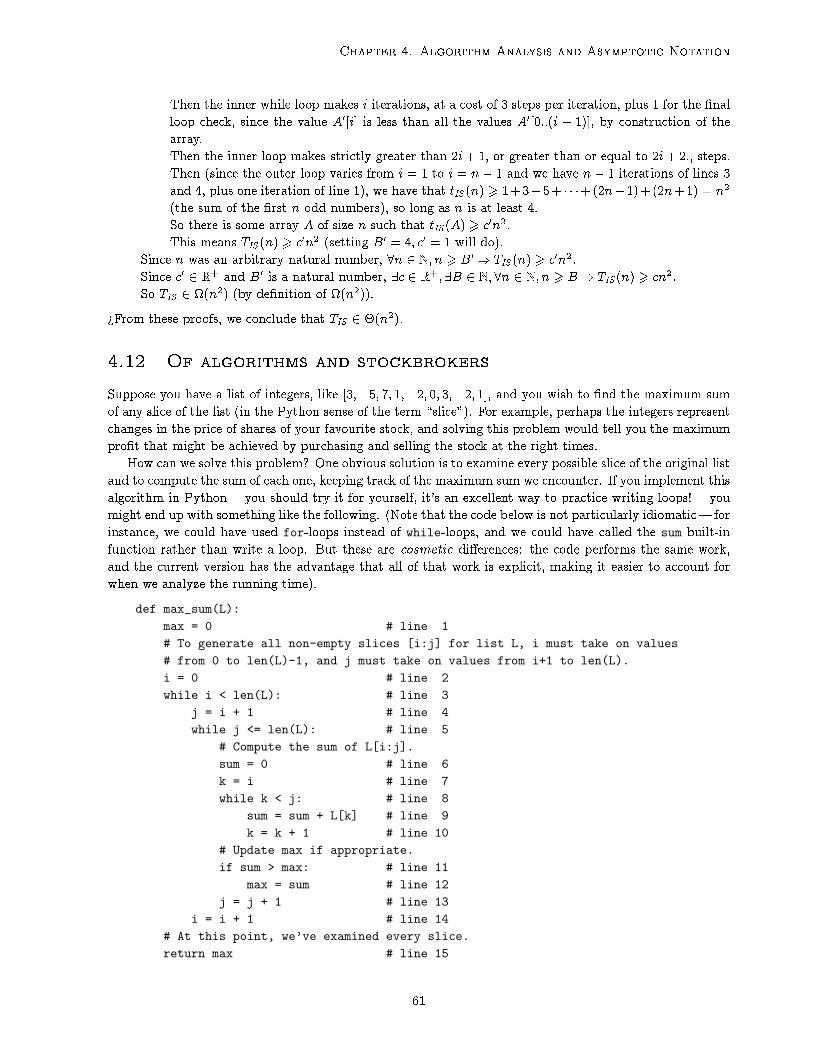
Chapter 4. Algorithm Analysis and Asymptotic Notation

Then the inner while loop makes i iterations, at a cost of 3 steps per iteration, plus 1 for the �nal

loop check, since the value A0[i] is less than all the values A0[0::(i � 1)], by construction of the

array.

Then the inner loop makes strictly greater than 2i+ 1, or greater than or equal to 2i+ 2., steps.

Then (since the outer loop varies from i = 1 to i = n� 1 and we have n� 1 iterations of lines 3

and 4, plus one iteration of line 1), we have that tIS (n) > 1+3+5+ � � �+(2n�1)+(2n+1) = n2

(the sum of the �rst n odd numbers), so long as n is at least 4.

So there is some array A of size n such that tIS (A) > c0n2.

This means TIS (n) > c0n2 (setting B0 = 4; c0 = 1 will do).

Since n was an arbitrary natural number, 8n 2 N; n > B0) TIS (n) > c0n2.

Since c0 2 R+ and B0 is a natural number, 9c 2 R+; 9B 2 N; 8n 2 N; n > B) TIS (n) > cn2.

So TIS 2 (n2) (by de�nition of (n2)).

>From these proofs, we conclude that TIS 2 �(n2).

4.12 Of algorithms and stockbrokers

Suppose you have a list of integers, like [3;�5; 7; 1;�2; 0; 3;�2; 1], and you wish to �nd the maximum sum

of any slice of the list (in the Python sense of the term \slice"). For example, perhaps the integers represent

changes in the price of shares of your favourite stock, and solving this problem would tell you the maximum

pro�t that might be achieved by purchasing and selling the stock at the right times.

How can we solve this problem? One obvious solution is to examine every possible slice of the original list

and to compute the sum of each one, keeping track of the maximum sum we encounter. If you implement this

algorithm in Python|you should try it for yourself, it's an excellent way to practice writing loops!|you

might end up with something like the following. (Note that the code below is not particularly idiomatic| for

instance, we could have used for-loops instead of while-loops, and we could have called the sum built-in

function rather than write a loop. But these are cosmetic di�erences: the code performs the same work,

and the current version has the advantage that all of that work is explicit, making it easier to account for

when we analyze the running time).

def max_sum(L):

max = 0 # line 1

# To generate all non-empty slices [i:j] for list L, i must take on values

# from 0 to len(L)-1, and j must take on values from i+1 to len(L).

i = 0 # line 2

while i < len(L): # line 3

j = i + 1 # line 4

while j <= len(L): # line 5

# Compute the sum of L[i:j].

sum = 0 # line 6

k = i # line 7

while k < j: # line 8

sum = sum + L[k] # line 9

k = k + 1 # line 10

# Update max if appropriate.

if sum > max: # line 11

max = sum # line 12

j = j + 1 # line 13

i = i + 1 # line 14

# At this point, we’ve examined every slice.

return max # line 15

61

Course notes for csc 165 h

The correctness of this code should be fairly obvious from the comments, except perhaps for one thing: what

if the input L is a list that contains only negative integers, like [�2;�1;�2;�3]? Shouldn't the maximum

sum of a slice be some negative integer, like �1? So why do we initialize max to 0?13

Now, let's analyze the worst-case running time of max_sum. Intuitively, T (n) 2 O(n3) (where n = len(L))

because of the triply-nested loops, each one of which iterates no more than n times. Is T (n) 2 (n3)? This

is perhaps not so obvious, but we will show that it is indeed the case. To begin the analysis, we must decide

exactly which operations to count and how much to count for each one. We must strike a balance: if our

counting is too �ne-grained, we risk getting bogged down in arithmetic that is irrelevant; if it is too coarse,

we risk ignoring signi�cant fractions of the work carried out by the algorithm. Given how the algorithm is

written, a reasonable middle ground is to count one \step" for each line of code that is executed.

T (n) 2 O(n3)

Analyzing the loops inside-out, we �nd that:

� The loop on lines 8{10 iterates j� i times (once for each value of k = i; i+1; : : : ; j�1). And j� i 6 n

(since j 6 n and i > 0). And the loop executes 3 steps at each iteration. So the innermost loop

executes no more than 3n steps.

� The loop on lines 5{13 iterates n� i times (once for each value of j = i+1; i+2; : : : ; n). And n� i 6 n

(since i > 0). And the loop executes at most 7 + 3n steps at each iteration: lines 5, 6, 7, 8, 11, 12,

13 each execute at most once, in addition to the 6 3n steps executed by the inner loop (line 5 always

executes one more time than the number of iterations of the inner loop, when the loop condition

becomes false; line 12 may or may not execute, but it certainly executes no more than once for each

iteration). So the middle loop executes at most 7n+ 3n2 steps.

� The loop on lines 3{14 iterates n times (once for each value of i = 0; 1; : : : ; n � 1). And the loop

executes at most 4 + 7n + 3n2 steps at each iteration: lines 3, 4, 5, 14 each execute at most once, in

addition to the 6 7n + 3n2 steps executed by the middle loop. So the outer loop executes no more

than 4n+ 7n2 + 3n3 steps.

� Lines 1, 2, 3, and 15 each execute once, so the algorithm executes 6 4+ 4n+7n2+3n3 steps in total,

for every input list L.

Now we are ready to write the proof formally.

Assume n 2 N and n > 1 and L is a list with len(L) = n.

As argued above, lines 8{10 perform at most 3n steps.

Then lines 5{13 perform at most (7 + 3n) � n 6 10n2 steps (as argued above).

Then lines 3{14 perform at most (4 + 10n2) � n 6 14n3 steps (as argued above).

Then the entire algorithm performs at most 4 + 14n3 6 18n3 steps.

Since n and L were arbitrary, 8n 2 N; n > 1) T (n) 6 18n3.

Hence 9c 2 R+; 9B 2 N; 8n 2 N; n > B) T (n) 6 cn3, i.e., T (n) 2 O(n3).

(Note that this proof really is not complete without the rough work above, which we simply did not bother

to repeat.)

T (n) 2 (n3)

The algorithm has three nested loops, so it's tempting to think that it is \obvious" that the running time is

(n3). But consider this: there are many pairs i; j for which the loop for k performs few iterations (when

j � i is small), so we are over-counting when we say that the loop for k performs \at most" n iterations.

The question is: by how much are we over-counting?

62

Chapter 4. Algorithm Analysis and Asymptotic Notation

To show that T (n) 2 (n3), we have to convince ourselves that the loop over k really does iterate at

least some fraction of n times, for at least some fraction of n2 many pairs i; j. There are many ways to do

this; here is one that is relatively simple (splitting up the range of values for i; j; k evenly).

� The loop over i iterates at least dn=3e times| for each of the values i = 0; 1; : : : ; dn=3e. (Really, weknow it performs more than this many iterations, but since we're working on proving a lower bound

it's okay to under-estimate here|we'll soon see why it makes sense to under-estimate in this way.)

� For each of these iterations of the outer loop i, the loop for j iterates at least dn=3e times| for each

of the values j = n�dn=3e+1; : : : ; n. (Again, we know that the loop really performs more work than

this but we're deliberately ignoring some of the work in order to guarantee a certain range of values

for k, in the quest for our lower bound.)

� For each of these pairs i; j, the inner loop for k iterates over the values i; i + 1; : : : ; j � 1. This will

always be at least dn=3e many iterations, since i 6 dn=3e and j > n�dn=3e+1. And each iteration of

the innermost loop performs at least 1 step (more than that, really, but again we're under-estimating).

Formally, assume n 2 N and n > 3.

Let L = [1; 2; : : : ; n]. Then L is a list of length n.

As argued above, the call max_sum(L) performs at least dn=3e � dn=3e � dn=3e > n3=27 many steps.

Since this happens speci�cally for list L, T (n) > n3=27. # by de�nition of \worst-case"

Since n was arbitrary, 8n 2 N; n > 3) T (n) > n3=27.

Hence 9c 2 R+;9B 2 N; 8n 2 N; n > B) T (n) > cn3, i.e., T (n) 2 (n3).

Doing better

If you examine the algorithm, you might notice one somewhat obvious ine�ciency. In case you cannot see it,

or to con�rm that we're thinking of the same thing, try the following exercise: trace through the execution

of the algorithm on input L = [3;�5; 7; 1;�2; 0; 3;�2; 1], when i = 1 (with max = 7). You should notice

that the algorithm computes sum = L[1], then sum = L[1] + L[2], etc. But each time, it starts over: for

example, to compute L[1] + L[2] + � � � + L[5], the algorithm completely discards the previous value of sum

(equal to L[1] + L[2] + L[3] + L[4]) and starts adding L[1] and L[2] and. . . . We could save computing time

if we kept the old value and simply added L[5] to it!

The general idea is to add values to a running total every time that the value of j changes, instead of

having a separate inner loop. See if you can implement this change on your own. You might end up with

something like the following.

def faster_max_sum(L):

max = 0 # line 1

# Generate all non-empty slices [i:j+1] for list L, where i takes on values

# from 0 to len(L)-1, and j takes on values from i to len(L)-1.

i = 0 # line 2

while i < len(L): # line 3

sum = 0 # line 4

j = i # line 5

while j < len(L): # line 6

sum = sum + L[j] # line 7

if sum > max: # line 8

max = sum # line 9

j = j + 1 # line 10

i = i + 1 # line 11

# At this point, we’ve examined every slice.

return max # line 12

63

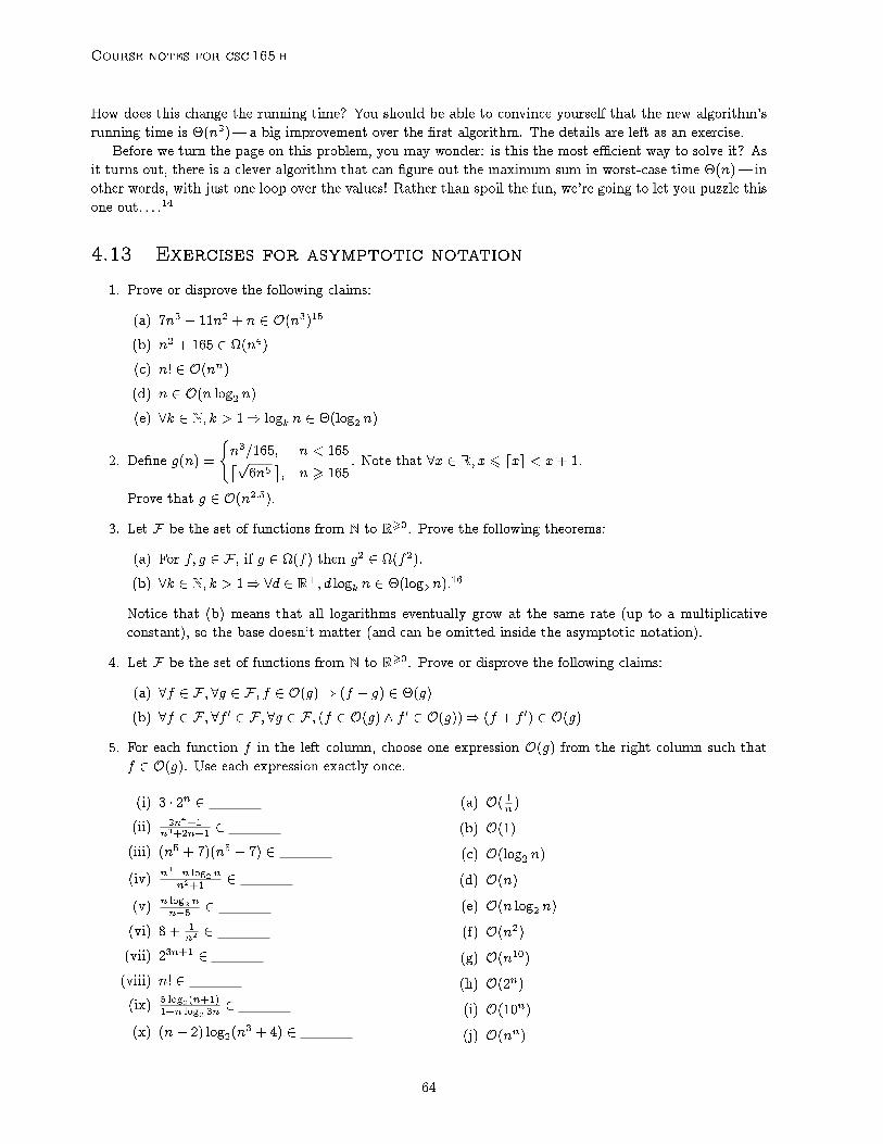
Course notes for csc 165 h

How does this change the running time? You should be able to convince yourself that the new algorithm's

running time is �(n2)|a big improvement over the �rst algorithm. The details are left as an exercise.

Before we turn the page on this problem, you may wonder: is this the most e�cient way to solve it? As

it turns out, there is a clever algorithm that can �gure out the maximum sum in worst-case time �(n)| in

other words, with just one loop over the values! Rather than spoil the fun, we're going to let you puzzle this

one out. . . .14

4.13 Exercises for asymptotic notation

1. Prove or disprove the following claims:

(a) 7n3 + 11n2 + n 2 O(n3)15

(b) n2 + 165 2 (n4)

(c) n! 2 O(nn)(d) n 2 O(n log2 n)(e) 8k 2 N; k > 1) logk n 2 �(log2 n)

2. De�ne g(n) =

(n3=165; n < 165�p

6n5�; n > 165

. Note that 8x 2 R; x 6 dxe < x+ 1.

Prove that g 2 O(n2:5).

3. Let F be the set of functions from N to R>0. Prove the following theorems:

(a) For f; g 2 F , if g 2 (f) then g2 2 (f2).

(b) 8k 2 N; k > 1)8d 2 R+; d logk n 2 �(log2 n).16

Notice that (b) means that all logarithms eventually grow at the same rate (up to a multiplicative

constant), so the base doesn't matter (and can be omitted inside the asymptotic notation).

4. Let F be the set of functions from N to R>0. Prove or disprove the following claims:

(a) 8f 2 F ;8g 2 F ; f 2 O(g)) (f + g) 2 �(g)

(b) 8f 2 F ;8f 0 2 F ; 8g 2 F ; (f 2 O(g) ^ f 0 2 O(g))) (f + f 0) 2 O(g)5. For each function f in the left column, choose one expression O(g) from the right column such that

f 2 O(g). Use each expression exactly once.

(i) 3 � 2n 2(ii) 2n4+1

n3+2n�1 2(iii) (n5 + 7)(n5 � 7) 2(iv) n4�n log

2n

n2+1 2(v) n log

2n

n�5 2(vi) 8 + 1

n2 2(vii) 23n+1 2(viii) n! 2(ix) 5 log

2(n+1)

1+n log23n 2

(x) (n� 2) log2(n3 + 4) 2

(a) O( 1n )(b) O(1)(c) O(log2 n)(d) O(n)(e) O(n log2 n)(f) O(n2)

(g) O(n10)

(h) O(2n)(i) O(10n)(j) O(nn)

64

Chapter 4. Algorithm Analysis and Asymptotic Notation

4.14 Exercises for algorithm analysis

1. Write a detailed analysis of the worst-case running time of algorithm faster_max_sum.

2. Write a detailed analysis of the worst-case running time of the following algorithm.

def mystery1(L):

""" L is a non-empty list of length len(L) = n. """

tot = 0

i = 0

while i < len(L):

if L[i] > 0:

tot = tot + L[i]

i = i + 1

return tot

3. Write a detailed analysis of the worst-case running time of the following algorithm.

def mystery2(L):

""" L is a non-empty list of length len(L) = n. """

i = 1

while i < len(L) - 1:

j = i - 1

while j <= i + 1:

L[j] = L[j] + L[i]

j = j + 1

i = i + 1

4. Write a detailed analysis of the worst-case running time of the following algorithm.

def mystery3(L):

""" L is a non-empty list of length len(L) = n. """

i = 1

while i < len(L):

print L[i]

i = i * 2

5. Write a detailed analysis of the worst-case running time of the following algorithm.

def mystery4(L):

""" L is a non-empty list of length len(L) = n. """

i = 0

while i < len(L):

if L[i] % 2 == 0:

j = i

while j < len(L):

L[j] = L[j] + 1

j = j + 1

i = i + 1

65

Course notes for csc 165 h

4.15 Induction interlude

Suppose P (n) is some predicate of the natural numbers, and:

(�) P (0) ^ (8n 2 N; P (n)) P (n+ 1)):

You should certainly be able to show that (�) implies P (0), P (1), P (2), in fact P (n) where n is any natural

number you have the patience to follow the chain of results to obtain. In fact, we feel that we can \turn the

crank" enough times to show that (�) implies P (n) for any natural number n. This is called the Principle

of Simple Induction (PSI). It isn't proved, it is an axiom that we assume to be true.

Here's an application of the PSI to some functions we've encountered before.

P (n): 2n > 2n.

I'd like to prove that 8n; P (n), using the PSI. Here's what I do:

Prove P (0): P (0) states that 20 = 1 > 2(0) = 0, which is true.

Prove 8n 2 N; P (n)) P (n+ 1):

Assume n 2 N. # arbitrary natural number

Assume P (n), that is 2n > 2n. # antecedent

Then n = 0 _ n > 0. # natural numbers are non-negative

Case 1 (assume n = 0): Then 2n+1 = 21 = 2 > 2(n+ 1) = 2.

Case 2 (assume n > 0): Then n > 1. # n is an integer greater than 0

Then 2n > 2. # since n > 1, and 2n is monotone increasing

Then 2n+1 = 2n + 2n > 2n+ 2 = 2(n+ 1). # by previous line and IH P (n)

Then 2n+1 > 2(n+ 1), which is P (n+ 1). # true in both possible cases

Then P (n)) P (n+ 1). # introduce )Then 8n 2 N; P (n)) P (n+ 1). # introduce 8

I now conclude, by the PSI, 8n 2 N; P (n), that is 2n > 2n.

What happens to induction for predicates that are true for all natural numbers after a certain point, but

untrue for the �rst few natural numbers? For example, 2n grows much more quickly than n2, but 23 is not

larger than 32. Choose n big enough, though, and it is true that:

P (n) : 2n > n2:

You can't prove this for all n, when it is false for n = 2; n = 3, and n = 4, so you'll need to restrict the

domain and prove that for all natural numbers greater than 4, P (n) is true. We don't have a slick way to

restrict domains in our symbolic notation. Let's consider three ways to restrict the natural numbers to just

those greater than 4, and then use induction.

Restrict by set difference: One way to restrict the domain is by set di�erence:

8n 2 N n f0; 1; 2; 3; 4g; P (n)

Again, we'll need to prove P (5), and then that 8n 2 N n f0; 1; 2; 3; 4g; P (n)) P (n+ 1).

Restrict by translation: We can also restrict the domain by translating our predicate, by lettingQ(n) =

P (n+ 5), that is:

Q(n) : 2n+5 > (n+ 5)2

Now our task is to prove Q(0) is true and that for all n 2 N, Q(n))Q(n+1). This is simple induction.

66

Chapter 4. Algorithm Analysis and Asymptotic Notation

Restrict using implication: Another method of restriction uses implication to restrict the domain where

we claim P (n) is true| in the same way as for sentences:

8n 2 N; n > 5) P (n):

The expanded predicate Q(n) : n > 5) P (n) now �ts our pattern for simple induction, and all we

need to do is prove:

1. Q(0) is true (it is vacuously true, since 0 > 5 is false).

2. 8n 2 N; Q(n))Q(n+ 1). This breaks into cases.

� If n < 4, then Q(n) and Q(n+1) are both vacuously true (the antecedents of the implication

are false, since n and n+1 are not greater than, nor equal to, 5), so there is nothing to prove.

� If n = 4, then Q(n) is vacuously true, but Q(n+1) has a true antecedent (5 > 5), so we need

to prove Q(5) directly: 25 > 52 is true, since 32 > 25.

� If n > 4, we can depend on the assumption of the consequent of Q(n� 1) being true to prove

Q(n):

2n = 2n�1 + 2n�1 (de�nition of 2n)

> 2(n� 1)2 (antecedent of Q(n� 1))

= 2n2 � 2n+ 2 = n2 + n(n� 2) + 2 > n2 + 2 > n2 (since n > 4 > 2)

After all that work, it turns out that we need prove just two things:

1. P (5)

2. 8n 2 N, If n > 4, then P (n)) P (n+ 1).

This is the same as before, except now our base case is P (5) rather than P (0), and we get to use the fact

that n > 5 in our induction step (if we need it).

Whichever argument you're comfortable with, notice that simple induction is basically the same: you

prove the base case (which may now be greater than 0), and you prove the induction step.

Chapter 4 Notes

1From 0 to (2� 1), if we work in analogy with base 10.

2To parse the 0:101 part, calculate 0:101 = 1(2�1) + 0(2�2) + 1(2�3).

3You should be able to look up this algorithm in an elementary school textbook.

4Same as the previous exercise, but only write numbers that have 0's and 1's, and do binary addition.

5Integer divide by 10.

6Integer divide by 2.

7Better in the sense of time complexity.

8Applying l'Hopital's Rule, limn!1

2n

n = limn!1

ln(2)�2n

1 =1, because limn!1 2n = limn!1 n =1.

9Sure, f = n2, g = 3n2 + 2.

67

Course notes for csc 165 h

10Sure. f and g don't need to both be monotonic, so let f(n) = n2 and

g(n) =

(n; n even

n3; n odd

So not every pair of functions from N! R>0 can be compared using Big-O.

11Let's try the symmetrical presentation of bi-implication.

12but not particularly e�cient. . .

13Don't forget the empty slice L[0 : 0] (or L[i : i] for any index i, for that matter). This is a valid slice

for any list and its sum is 0, which is greater than any negative integer.

14Hint: you don't need a loop to �gure out the maximum sum of any slice that ends at index i.

15The claim is true.

Let c0 = 8. Then c0 2 R+.

Let B0 = 12. Then B0 2 N.Assume n 2 N and n > B0.

Then n3 = n � n2 > 12 � n2 = 11n2 + n2 > 11n2 + n. # since n > B0 = 12

Thus c0n3 = 8n3 = 7n3 + n3 > 7n3 + 11n2 + n.

So 8n 2 N, n > B0) 7n3 + 11n2 + n 6 c0n3.

Since B0 is a natural number, 9B 2 N; 8n 2 N; n > B) 7n3 + 11n2 + n 6 c0n3.

Since c0 is a real positive number, 9c 2 R+;9B 2 N; 8n 2 N; n > B) 7n3 + 11n2 + n 6 cn3.

By de�nition, 7n3 + 11n2 + n 2 O(n3).

16Assume k 2 N and k > 1.

Assume d 2 R+.

It su�ces to argue that d logk n 2 �(log2 n).

Let c01 =d

log2k . Since k > 1, log2 k 6= 0 and so c01 2 R+.

Let c02 =d

log2k . By the same reasoning, c02 2 R+.

Let B0 = 1. Then B0 2 N.Assume n 2 N and n > B0.

Then c01 log2 n = dlog

2k log2 n = d log

2n

log2k = d logk n 6 d logk n.

Moreover, d logk n 6 d log2n

log2k = d

log2k log2 n = c02 log2 n.

Hence, 8n 2 N; n > B0) c01 log2 n 6 d logk n 6 c02 log2 n.

Thus 9c1 2 R+; 9c2 2 R+; 9B 2 N; 8n 2 N; n > B) c1 log2 n 6 d logk n 6 c2 log2 n.

By de�nition, d logk n 2 �(log2 n).

Thus, 8d 2 R+; d logk n 2 �(log2 n).

Hence 8k 2 N; k > 1)8d 2 R+; d logk n 2 �(log2 n).

68

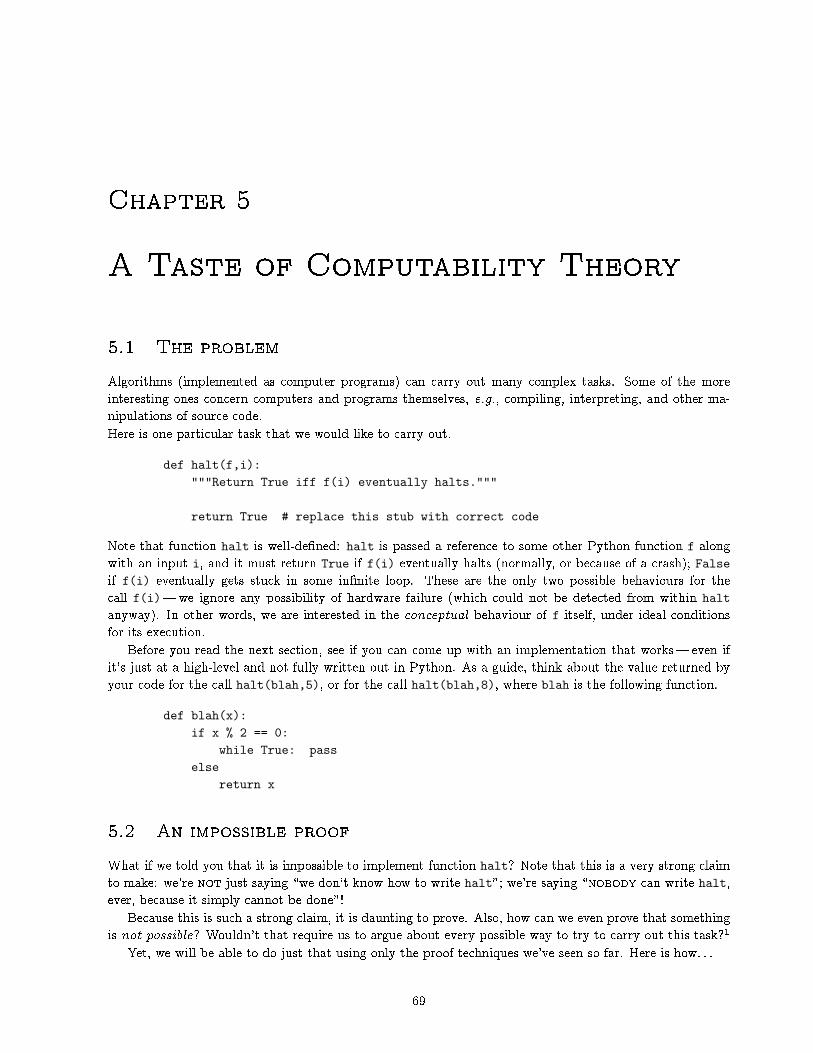
Chapter 5

A Taste of Computability Theory

5.1 The problem

Algorithms (implemented as computer programs) can carry out many complex tasks. Some of the more

interesting ones concern computers and programs themselves, e.g., compiling, interpreting, and other ma-

nipulations of source code.

Here is one particular task that we would like to carry out.

def halt(f,i):

"""Return True iff f(i) eventually halts."""

return True # replace this stub with correct code

Note that function halt is well-de�ned: halt is passed a reference to some other Python function f along

with an input i, and it must return True if f(i) eventually halts (normally, or because of a crash); False

if f(i) eventually gets stuck in some in�nite loop. These are the only two possible behaviours for the

call f(i)|we ignore any possibility of hardware failure (which could not be detected from within halt

anyway). In other words, we are interested in the conceptual behaviour of f itself, under ideal conditions

for its execution.

Before you read the next section, see if you can come up with an implementation that works|even if

it's just at a high-level and not fully written out in Python. As a guide, think about the value returned by

your code for the call halt(blah,5), or for the call halt(blah,8), where blah is the following function.

def blah(x):

if x % 2 == 0:

while True: pass

else

return x

5.2 An impossible proof

What if we told you that it is impossible to implement function halt? Note that this is a very strong claim

to make: we're not just saying \we don't know how to write halt"; we're saying \nobody can write halt,

ever, because it simply cannot be done"!

Because this is such a strong claim, it is daunting to prove. Also, how can we even prove that something

is not possible? Wouldn't that require us to argue about every possible way to try to carry out this task?1

Yet, we will be able to do just that using only the proof techniques we've seen so far. Here is how. . .

69

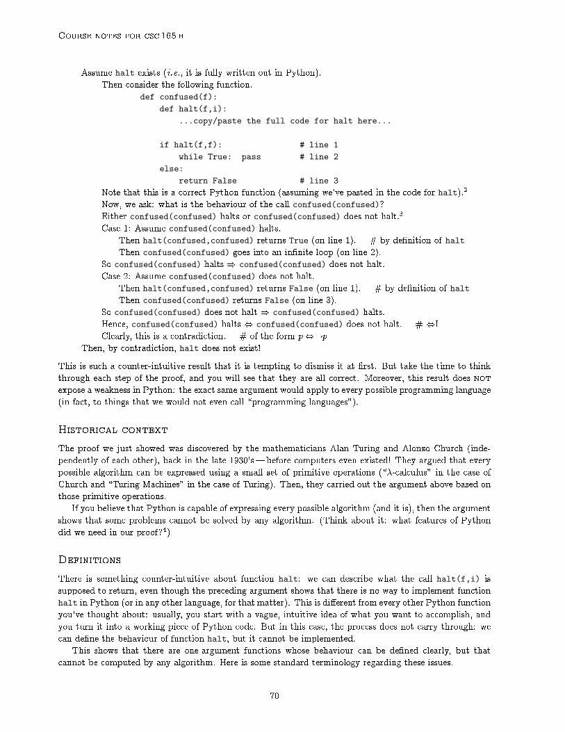
Course notes for csc 165 h

Assume halt exists (i.e., it is fully written out in Python).

Then consider the following function.

def confused(f):

def halt(f,i):

...copy/paste the full code for halt here...

if halt(f,f): # line 1

while True: pass # line 2

else:

return False # line 3

Note that this is a correct Python function (assuming we've pasted in the code for halt).2

Now, we ask: what is the behaviour of the call confused(confused)?

Either confused(confused) halts or confused(confused) does not halt.3

Case 1: Assume confused(confused) halts.

Then halt(confused,confused) returns True (on line 1). # by de�nition of halt

Then confused(confused) goes into an in�nite loop (on line 2).

So confused(confused) halts ) confused(confused) does not halt.

Case 2: Assume confused(confused) does not halt.

Then halt(confused,confused) returns False (on line 1). # by de�nition of halt

Then confused(confused) returns False (on line 3).

So confused(confused) does not halt ) confused(confused) halts.

Hence, confused(confused) halts , confused(confused) does not halt. # ,I

Clearly, this is a contradiction. # of the form p,:pThen, by contradiction, halt does not exist!

This is such a counter-intuitive result that it is tempting to dismiss it at �rst. But take the time to think

through each step of the proof, and you will see that they are all correct. Moreover, this result does not

expose a weakness in Python: the exact same argument would apply to every possible programming language

(in fact, to things that we would not even call \programming languages").

Historical context

The proof we just showed was discovered by the mathematicians Alan Turing and Alonzo Church (inde-

pendently of each other), back in the late 1930's|before computers even existed! They argued that every

possible algorithm can be expressed using a small set of primitive operations (\�-calculus" in the case of

Church and \Turing Machines" in the case of Turing). Then, they carried out the argument above based on

those primitive operations.

If you believe that Python is capable of expressing every possible algorithm (and it is), then the argument

shows that some problems cannot be solved by any algorithm. (Think about it: what features of Python

did we need in our proof?4)

Definitions

There is something counter-intuitive about function halt: we can describe what the call halt(f,i) is

supposed to return, even though the preceding argument shows that there is no way to implement function

halt in Python (or in any other language, for that matter). This is di�erent from every other Python function

you've thought about: usually, you start with a vague, intuitive idea of what you want to accomplish, and

you turn it into a working piece of Python code. But in this case, the process does not carry through: we

can de�ne the behaviour of function halt, but it cannot be implemented.

This shows that there are one-argument functions whose behaviour can be de�ned clearly, but that

cannot be computed by any algorithm. Here is some standard terminology regarding these issues.

70

Chapter 5. A Taste of Computability Theory

Definition: A function f : A! B is computable if it can be implemented in Python, i.e., if there exists

a Python function f such that for all a 2 A, f(a) returns the value of f(a).

Functions for which this is not possible (e.g., halt) are called non-computable. Note that this de�nition

applies only to well-de�ned mathematical functions f : A! B|those for which there is exactly one value

f(a) for every a 2 A. The distinction between \computable" and \non-computable" has nothing to do with

the de�nition of the function f . Rather, it distinguishes between functions whose values can be calculated

by an algorithm, and those for which this is not possible.

5.3 Reductions

So halt is not computable. But it's not the end of the world if this one function cannot be computed, is it?

Unfortunately, non-computable functions are like bugs: when you discover one, you quickly realize that

there are many more around. . . In this section, we'll explain how to use the fact that halt is not computable,

to show that other functions are also non-computable.

For example, consider the function initialized(f,v), whose value is True when variable v is guaranteed

to be initialized before its �rst use, whenever Python function f is called (no matter what input is passed

to f)| initialize(f,v) is False if there is even one input i such that the call f(i) attempts to use the

value of v before it has been initialized. Note that there is a subtle, but important, distinction to be made:

we don't want initialized(f,v) to be True when there is just a possibility that variable v may be used

before its initialization in f|we want to know that this actually happens during the call f(i) for some

input i. For example, consider the following functions:

def f1(x): def f2(x):

return x + 1 return x + y + 1

print y

While it is the case that f1 contains a statement that uses variable y before it is initialized, this statement

can never actually be executed|so initialized(f1,y) is True, vacuously. On the other hand, variable y

is actually used before its initialization in f2|so initialized(f2,y) is False.

Claim 5.1: The function initialized is non-computable.

Proof:

For a contradiction, assume that initialized is computable, i.e., it can be implemented as a Python

function.

We want to show that this assumption leads to a contradiction. More speci�cally in this case, we

want to reach the contradiction that halt is computable. So, consider the following program.

def halt(f,i):

def initialized(g,v):

...code for initialized goes here...

# Put some code here to scan the code for f and figure out

# a variable name ’v’ that does not appear anywhere in f.

def f_prime(x):

# Ignore the argument x, call f with the fixed argument i

# (the one passed in to halt).

f(i)

print v

return not initialized(f_prime,v)

71

Course notes for csc 165 h

(Although we left out some of the details in this code|the part that is commented out| it can

be �lled in and the result is a valid Python program|assuming that the code for initialized

can be �lled-in, of course.)

If f(i) halts, then f_prime(i) will execute the statement print v, so initialized(f_prime,v)

returns False and halt(f,i) returns True.

If f(i) does not halt, then f_prime(x) never executes print v (no matter what value x has), so

initialized(f_prime,v) returns True and halt(f,i) returns False.

But there is no Python implementation of function halt, as we've already shown!

Hence, there is no Python implementation of function initialized.

Let's step through the preceding argument to better understand it.

� We want to prove that initialized is non computable (i.e., that there is no Python code to compute

it), based on the fact that halt is non-computable.

We decide to use a proof by contradiction, so we begin by assuming that initialized is computable.

Our goal is now to derive a contradiction. An obvious candidate is the statement: \halt is com-

putable."

� To show that halt is computable means to show that there exists an algorithm to compute it. The

easiest way to achieve this is to describe an explicit algorithm for halt.

In other words, our goal is to �nd a way to compute halt, given a supposed algorithm for initialized.

� The trick to achieving this is contained in the de�nition of function f_prime in the argument: this

function is valid Python code and it has been de�ned with the property that the call f(i) halts i�

variable v is used without being initialized in f_prime.

Moreover, this property does not depend on our knowledge of whether or not f(i) halts.

� Hence, we know that our implementation of halt will return the correct value, under the assumption

that initialized has been implemented correctly.

� The contradiction follows immediately, which concludes the proof.

Note that the critical step in this argument|the one that requires the most creativity and insight| is

to �nd a way to tie together the fact that \the call f(i) halts" with the fact that \variable v is always

initialized before its use within function f_prime." Once we �gure out how to achieve this, the structure of

the rest of the proof is straightforward.

This kind of argument is called a reduction and can be used to show that many other functions are

non-computable, by proving conditional statements of the form:

If f is computable (i.e., there is a Python function f that computes f), then h is also computable

(i.e., we can write a python function h that computes h).

Picking h to be a function known to be non-computable (like halt) immediately gives us that f is also

non-computable, by contrapositive.

5.4 Countability

The idea for function confused in the proof that halt is non-computable is an example of a diagonaliza-

tion argument, �rst used by the mathematician Georg Cantor to show that the set of real numbers is larger

than the set of natural numbers.

Now that, in itself, may seem like a strange statement to make: how can the set of real numbers be

\larger" than the set of natural numbers? Don't they both contain in�nitely many numbers? What does it

even mean to compare the sizes of in�nitely large sets?

72

Chapter 5. A Taste of Computability Theory

Let's take things one step at a time and scale back to simpler in�nite sets. Consider N (the set of natural

numbers) and Z (the set of integers). Between the two, which set is larger? The answer seems obvious: Z

contains N as proper subset, so Z must be larger.

But now think about this: which set has larger size? Now the answer is not so obvious: for �nite sets

\size" is a natural number, but how do we measure the size of in�nite sets? Adding or removing one element

from an in�nite set does not change its size: it's still in�nite. So are all in�nite sets the same size? And

what does \in�nite size" even mean?

Let's think through this more carefully. When we count the elements in a set, what we are really doing

is associating a number with each element : you can easily imagine yourself pointing to elements one after

the other while saying \one, two, three, . . . " The easiest way to formalize this idea involves the notions of

one-to-one and onto functions.

Definition: Suppose f : A! B (i.e., f is a function that associates an element f(a) 2 B to each element

a 2 A). Then we say that

� f is one-to-one if 8a1 2 A; 8a2 2 A; f(a1) = f(a2)) a1 = a2 (i.e., f gives distinct values to

di�erent elements of A);

� f is onto if 8b 2 B; 9a 2 A; f(a) = b (i.e., every element in B can be \reached" from at least

one element of A).

For example,

� the function f : N! N de�ned by f(x) = bx=2c+ 2 is neither one-to-one (f(2) = 3 = f(3)) nor onto

(there is no x 2 N such that f(x) = 1);

� the function f : N! N de�ned by f(x) = 2x is one-to-one (f(x) = f(y)) x = y) but not onto (there

is no x 2 N such that f(x) = 1);

� the function f : N! N de�ned by f(x) = bx=2c is not one-to-one (f(2) = 1 = f(3)) but it is onto (for

all n 2 N, f(2n) = n);

� the function f : N ! N de�ned by f(x) = 10 � x if x 6 10; f(x) = x otherwise is both one-to-one

(the numbers f0; : : : ; 10g get mapped to f10; : : : ; 0g and f11; 12; : : : g remain unchanged) and onto

(8n 2 N; (n 6 10) f(10� n) = n) ^ (n > 10) f(n) = n)).

(You can �nd out more about one-to-one and onto functions in Section 5.2 of Velleman's \How to Prove It,"

or on Wikipedia.)

Using these concepts, the idea of \counting" can be formalized as follows:

Definition: Set A is countable if

1. there is a function f : A! N that is one-to-one, or equivalently,

2. there is a function f : N! A that is onto.

For example,

Claim 5.2: Z is countable.

Let

f(n) =

(n=2 if n is even,

(1� n)=2 if n is odd.

Then f : N! Z.

Next, we show that f is onto.

73

Course notes for csc 165 h

Assume x 2 Z.Then x 6 0 or x > 0.

Case 1: Assume x 6 0.

Let n0 = 1� 2x.

Then x 6 0)�2x > 0) n0 > 0 so n0 2 N.Also, n0 = 2(�x) + 1 so n0 is odd.

Then f(n0) = (1� n0)=2 = (1� (1� 2x))=2 = 2x=2 = x.

Hence 9n 2 N; f(n) = x.

Case 2: Assume x > 0.

Let n0 = 2x.

Then x > 0) n0 > 0 so n0 2 N.Also, n0 = 2x is even.

Then f(n0) = n0=2 = 2x=2 = x.

Hence 9n 2 N; f(n) = x.

In all cases, 9n 2 N; f(n) = x.

Since x was arbitrary, 8x 2 Z; 9n 2 N; f(n) = x, i.e., f is onto. (Note that f is not one-to-one|can

you see why?5)

Hence, there is a function f : N! Z that is onto, i.e., Z is countable.

Informally, we often show that a set A is countable by giving an argument that it is possible to list every

element in the set| this corresponds to giving a function f : N! A that is onto, though the function may

not be written out algebraically. What matters most is to make sure that there is some systematic way to

list the elements of A and that the list includes every element of A at least once.

For example, we may argue that Z is countable by exhibiting the following list (really, more a list pattern

because of the \. . . "):

Z : 0;�1; 1;�2; 2;�3; 3; : : :Implicitly, this de�nes a function f : N ! Z|just think of the list as an enumeration of f 's values

(f(0) = 0; f(1) = �1; f(2) = 1; : : : ) Once we see the pattern, it is obvious that the list includes every

possible integer, i.e., the implicit function f is onto. Hence, Z is countable.

What about �nite sets, e.g., fa; b; cg? Is it countable? Yes, because of condition 1 in the de�nition of

countability: the function f(a) = 1, f(b) = 2, f(c) = 3 is easily proved to be one-to-one.

Assume x; y 2 fa; b; cg and f(x) = f(y).

Then f(x) = f(y) = 1 or f(x) = f(y) = 2 or f(x) = f(y) = 3.

# these are the only values in the domain of f

Case 1: Assume f(x) = f(y) = 1.

Then x = y = a so x = y.

Case 2: Assume f(x) = f(y) = 2.

Then x = y = b so x = y.

Case 3: Assume f(x) = f(y) = 3.

Then x = y = c so x = y.

In every case, x = y.

Hence 8x 2 fa; b; cg; 8y 2 fa; b; cg; f(x) = f(y)) x = y, i.e., f is one-to-one.

What about other in�nite sets? Are they all countable? Consider the set Q of rational numbers (i.e.,

numbers of the form p=q for integers p; q with q 6= 0). Numerically, we know that this set is much di�erent

from Z or N: the rational numbers are dense (there are in�nitely many rational numbers between any two

other rational numbers). This di�erence might seem to imply that Q is not countable, for how could we

hope to list all of the rational numbers? However, note that our informal de�nition of countability does not

require that we be able to list the elements in any kind of numerical order| in fact, our list for Z above was

not ordered numerically.

74

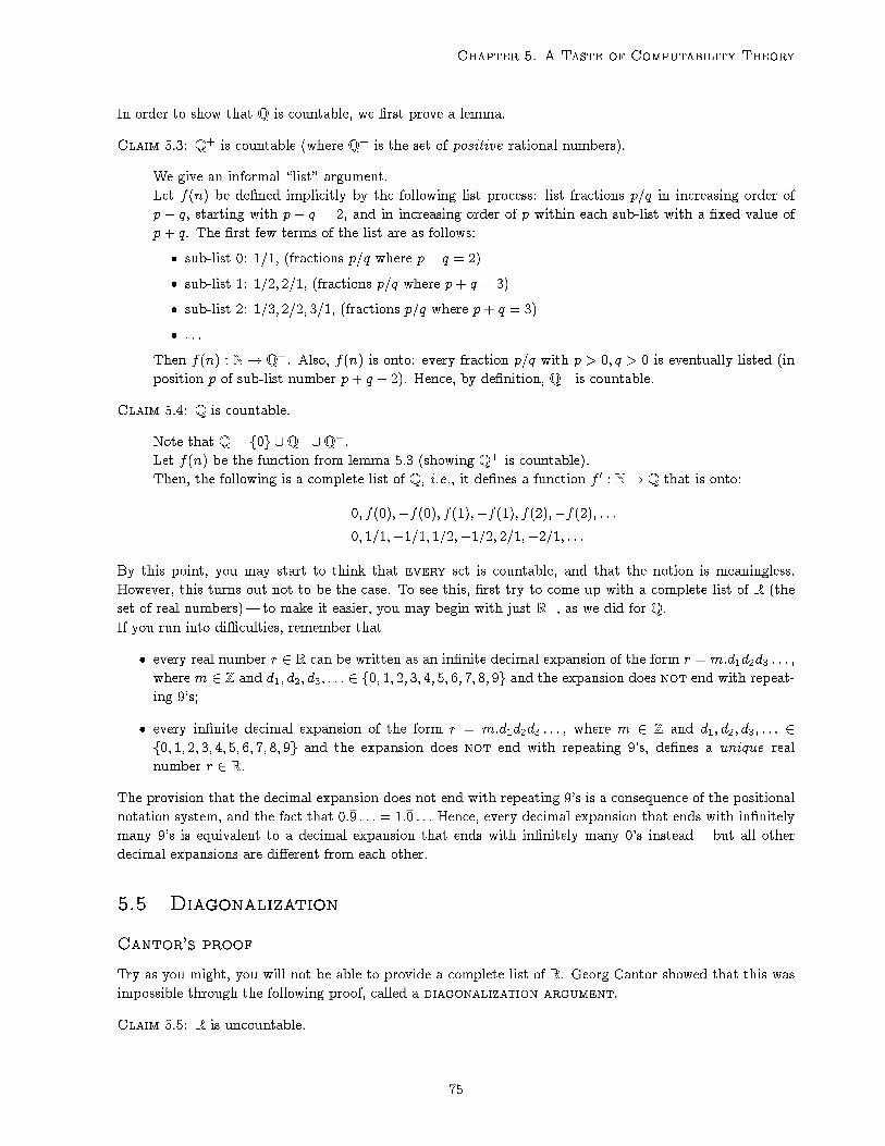
Chapter 5. A Taste of Computability Theory

In order to show that Q is countable, we �rst prove a lemma.

Claim 5.3: Q+ is countable (where Q+ is the set of positive rational numbers).

We give an informal \list" argument.

Let f(n) be de�ned implicitly by the following list process: list fractions p=q in increasing order of

p + q, starting with p + q = 2, and in increasing order of p within each sub-list with a �xed value of

p+ q. The �rst few terms of the list are as follows:

� sub-list 0: 1=1, (fractions p=q where p+ q = 2)

� sub-list 1: 1=2; 2=1, (fractions p=q where p+ q = 3)

� sub-list 2: 1=3; 2=2; 3=1, (fractions p=q where p+ q = 3)

� : : :

Then f(n) : N! Q+. Also, f(n) is onto: every fraction p=q with p > 0; q > 0 is eventually listed (in

position p of sub-list number p+ q � 2). Hence, by de�nition, Q+ is countable.

Claim 5.4: Q is countable.

Note that Q = f0g [Q� [Q+.

Let f(n) be the function from lemma 5.3 (showing Q+ is countable).

Then, the following is a complete list of Q, i.e., it de�nes a function f 0 : N! Q that is onto:

0; f(0);�f(0); f(1);�f(1); f(2);�f(2); : : := 0; 1=1;�1=1; 1=2;�1=2; 2=1;�2=1; : : :

By this point, you may start to think that every set is countable, and that the notion is meaningless.

However, this turns out not to be the case. To see this, �rst try to come up with a complete list of R (the

set of real numbers)| to make it easier, you may begin with just R+, as we did for Q.

If you run into di�culties, remember that

� every real number r 2 R can be written as an in�nite decimal expansion of the form r = m:d1d2d3 : : : ,

where m 2 Z and d1; d2; d3; : : : 2 f0; 1; 2; 3; 4; 5; 6; 7; 8; 9g and the expansion does not end with repeat-

ing 9's;

� every in�nite decimal expansion of the form r = m:d1d2d3 : : : , where m 2 Z and d1; d2; d3; : : : 2f0; 1; 2; 3; 4; 5; 6; 7; 8; 9g and the expansion does not end with repeating 9's, de�nes a unique real

number r 2 R.

The provision that the decimal expansion does not end with repeating 9's is a consequence of the positional

notation system, and the fact that 0:9 : : : = 1:0 : : : Hence, every decimal expansion that ends with in�nitely

many 9's is equivalent to a decimal expansion that ends with in�nitely many 0's instead|but all other

decimal expansions are di�erent from each other.

5.5 Diagonalization

Cantor's proof

Try as you might, you will not be able to provide a complete list of R. Georg Cantor showed that this was

impossible through the following proof, called a diagonalization argument.

Claim 5.5: R is uncountable.

75

Course notes for csc 165 h

Proof:

For a contradiction, assume that R is countable.

Then there is a function f : N! R that is onto. # by de�nition of \countable"

We can visualize function f as follows: for every natural number n 2 N, f(n) is a real number,

represented as an in�nite decimal expansion that does not end with repeating 9's:

f(0) = i0:d0;0 d0;1 d0;2 � � � d0;n � � �f(1) = i1:d1;0 d1;1 d1;2 � � � d1;n � � �f(2) = i2:d2;0 d2;1 d2;2 � � � d2;n � � �... =

...

f(n) = in:dn;0dn;1dn;2� � � dn;n� � �... =

...

where i0; i1; : : : 2 Z are the integer parts of the real numbers f(0); f(1); : : : , and 8i 2 N; 8j 2 N,di;j 2 f0; 1; 2; 3; 4; 5; 6; 7; 8; 9g.Now, let r = 0:d0d1d2 � � � dn � � � , where 8i 2 N,

di =

(1 if di;i = 0;

0 otherwise:

Then r 2 R. # r is an in�nite decimal that does not end with repeating 9's

Then 9k 2 N; f(k) = r. # f is onto

Since f(k) = ik:dk;0dk;1dk;2 � � � dk;n � � � and r = 0:d0d1d2 � � � dn � � � , this implies ik = 0 and 8n 2 N,

dk;n = dn =

(1 if dn;n = 0;

0 otherwise:

But then,

dk;k = dk =

(1 if dk;k = 0;

0 otherwise;

i.e., dk;k = 0, dk;k = 1, a contradiction!

Then, by contradiction, R is not countable.

Take the time to study this proof a little. . .

You should notice the following key elements:

� The construction of a real number r such that 8n 2 N; f(n) 6= r.

� The fact that this construction is carried out for an arbitrary function f : N! R.

You should be able to use these ideas to write a direct proof that there does not exist any function f : N! R

that is onto|thus proving directly that R is uncountable.

Diagonalization and computability

The construction of real number r in the last proof is done using diagonalization. The reason for this name

becomes obvious if we visualize how r is constructed: each digit di of r is de�ned to be di�erent from at

least one digit di;i in the decimal expansion of the real number f(i).

76

Chapter 5. A Taste of Computability Theory

r = 0: d0 d1 d2 � � � dn � � �f(0) = i0: d0;0 d0;1 d0;2 � � � d0;n � � �f(1) = i1: d1;0 d1;1 d1;2 � � � d1;n � � �f(2) = i2: d2;0 d2;1 d2;2 � � � d2;n � � �... =

...

f(n) = in: dn;0 dn;1 dn;2 � � � dn;n � � �... =

...

Because there are in�nitely many digits in the decimal expansion of r (one for each natural number n 2 N),r is di�erent from the real number f(n) for every n 2 N.

Now, remember that we started this discussion in the context of the proof that function halt cannot be

implemented in Python. Back then, I mentioned that this proof was an example of diagonalization| I will

now explain why.

First, notice that halt takes two arguments: a one-argument Python function f and an input i for f.

Clearly, there are in�nitely many one-argument Python functions f, but what kind of in�nity: countable

or uncountable? To answer this question, we need a speci�c point of view: remember that every Python

function can be written down as a text �le, i.e., a �nite sequence of characters, from a �xed set of characters.

To be speci�c, let's assume the character set is UTF-8, which contains 256 di�erent characters| the exact

details of the encoding used for the set of characters don't matter: what matters is that the set of possible

characters is �xed, i.e., the same �nite set of characters can be used to write down every possible Python

function. So, every Python function can be written down as a sequence of characters in UTF-8, and every

such sequence of characters is really just an integer in disguise: just treat each character as a \digit" in

base-256 notation.

If you think about it, what we've just done in the argument above is to de�ne a function

g : one-argument Python functions! N

that is one-to-one: di�erent Python functions get assigned to di�erent numbers, because their source code

must di�er by at least one character. So by de�nition, the set of one-argument Python functions is count-

able|actually, the argument is more general than this: it shows that the set of all Python programs is

countable.

By the de�nition of countability, this means that there is some other function

g0 : N! one-argument Python functions

that is onto, i.e., it is possible to list every one-argument Python function: g0(0); g0(1); g0(2); : : : |to make

the notation easier to understand, we'll use subscripts f0 = g0(0); f1 = g0(1); f2 = g0(2); : : : in the rest of the

argument.

Keep in mind that each fn is actually just a string : the source code for some one-argument Python

function. So it makes sense to consider the function call fi(fj) for i; j 2 N: we are simply calling the Python

function whose source code is given by fi with the string fj as argument.

Now, consider the following table of behaviours, where we list one-argument Python functions down the

left side and inputs for those functions across the top|our list only contains speci�c kinds of inputs (those

that are listings for one-argument Python functions), and it is therefore not a complete list of all possible

inputs. The entry at row fi and column fj states whether the call fi(fj) halts or not (the values shown

below are just an example).

77

Course notes for csc 165 h

f0 f1 f2 � � � fn � � �f0 halts halts loops � � � halts � � �f1 loops loops loops � � � halts � � �f2 loops halts halts � � � loops � � �...

...

fn halts halts halts � � � halts � � �...

...

(Note that, when we assume that halt can be coded up in Python, this implies that every entry in this table

can be computed by halt.) The function confused is created by a simple process of diagonalization over

the table: just use halt to �gure out the behaviour of fi(fi) and make confused do the opposite. If halt

exists, then so does confused, but confused cannot be any of the elements of the list f0; f1; f2; : : : |by

construction, its behaviour di�ers from each one of these functions. This is how we get a contradiction.

Note that this argument also shows that every list of one-argument functions is incomplete. If you look

at if again more carefully, you should see that the argument can be interpreted as a proof that the set of

one-argument functions (meaning functions' behaviours) is uncountable. Since we've already argued that

the set of Python programs is countable, this means there are uncountably many functions that cannot be

implemented in Python!

We've barely scratched the surface of this fascinating topic. If you �nd it interesting|and who

wouldn't!| then you can �nd out much more in the courses csc 463 h and csc 438 h.

Chapter 5 Notes

1Yes, it would. And it turns out to be possible to give just such an argument, as you'll see.

2Yes, Python does allow such \nested" function de�nitions: it simply makes halt de�ned locally within

confused, just like for variables.

3Notice this is just an application of Excluded Middle.

4Functions, conditionals, and loops. We used \nested functions," but that is not strictly necessary.

5f(0) = 0=2 = 0 = (1� 1)=2 = f(1).

78