Indian Institute of Technology, Kanpur

Department of Industrial and Management Engineering

IME672A Data Mining and Knowledge Discovery

Course Project Report

Authors:Ayush AgarwalGaurav VermaHarshit BishtSri Krishna Mannem

Group 8

Course Instructor:Dr. Faiz Hamid

June 29, 2016

Abstract

Customer churn is a recurrent problem in the telecommunications industry, with 2-4% of cus-tomers changing brands every month. The following project aims to take data from a telecom-munications company and use it to train classification models that will be able to predict futurechurn behavior of customers. The concepts of Data Preprocessing, Classification, and EnsembleMethods are applied for the same.

1

Contents

1 Overview 31.1 The Problem . . . . . . . . . . . . . . . . . . . . . . . . . . . . . . . . . . . . . . . . . 31.2 The Data . . . . . . . . . . . . . . . . . . . . . . . . . . . . . . . . . . . . . . . . . . . 31.3 Initial Impressions . . . . . . . . . . . . . . . . . . . . . . . . . . . . . . . . . . . . . . 3

2 Data Preprocessing 42.1 Basic Transformations . . . . . . . . . . . . . . . . . . . . . . . . . . . . . . . . . . . . 42.2 Handling Missing Values . . . . . . . . . . . . . . . . . . . . . . . . . . . . . . . . . . . 42.3 Visualizing Correlation among Attributes . . . . . . . . . . . . . . . . . . . . . . . . . 42.4 Dimensionality Reduction using Rough Sets . . . . . . . . . . . . . . . . . . . . . . . . 62.5 Training Set and Test Set . . . . . . . . . . . . . . . . . . . . . . . . . . . . . . . . . . 6

3 Classifiers 73.1 Decision Tree . . . . . . . . . . . . . . . . . . . . . . . . . . . . . . . . . . . . . . . . . 73.2 Naive Bayes Classifier . . . . . . . . . . . . . . . . . . . . . . . . . . . . . . . . . . . . 93.3 Logistic Regression Model . . . . . . . . . . . . . . . . . . . . . . . . . . . . . . . . . . 93.4 SVM . . . . . . . . . . . . . . . . . . . . . . . . . . . . . . . . . . . . . . . . . . . . . . 103.5 Neural Networks . . . . . . . . . . . . . . . . . . . . . . . . . . . . . . . . . . . . . . . 11

4 Ensemble Methods 11

5 Questions for Discussion 125.1 Describe your predictive churn model. What statistical technique did you use and why?

How did you select variables to be included in the model? Is your model adequate?Justify. . . . . . . . . . . . . . . . . . . . . . . . . . . . . . . . . . . . . . . . . . . . . . 12

5.2 Demonstrate the predictive performance of the model. Is the performance adequate? . 125.3 What are the key factors that predict customer churn? Do these factors make sense?

Why or why not? . . . . . . . . . . . . . . . . . . . . . . . . . . . . . . . . . . . . . . . 135.4 What offers should be made to which customers to encourage them to remain with

Cell2Cell? Assume that your objective is to generate net positive cash flow, i.e., gen-erate additional customer revenues after subtracting out the cost of the incentive. . . . 14

5.5 Assuming these actions were implemented, how would you determine whether theyhad worked? . . . . . . . . . . . . . . . . . . . . . . . . . . . . . . . . . . . . . . . . . . 14

2

1 Overview

1.1 The Problem

To avoid customer churn, the project aims to accurately predict whether a customer is going to churnsoon or not provided some information about him. The following sections will provide more insightinto how the same is achieved.

1.2 The Data

The customer data provided consists of 71047 records of 78 attributes in a csv file. Of the attributes,CALIBRAT separates the training data from the test data, and the other 77 attributes give detailsabout the customers. The attributes belong to 3 major logical categories:

• Attributes related to usage (REVENUE, MOU, ROAM etc.)

• Personal Attributes (AGE, INCOME, CHILDREN etc.)

• Attributes related to previous company contact (MAILORD, RETCALLS etc.)

The attributes can also be differentiated based on the type of data they contain. Namely:

• 37 Numerical Attributes (INCOME, REVENUE etc.)

• 40 Binary Attributes (CREDITA, CREDITAA etc.)

1.3 Initial Impressions

The data seemed suggestive, but not usable straightaway, especially given the large number of recordsthat had all the binary attributes used to store nominal/ordinal variables zero, meaning that theirvalue was unknown.

3

2 Data Preprocessing

Since Data Preprocessing has already been covered in Assignment 1, it will only be covered briefly,with only areas of interest receiving a detailed treatment. Statistical analysis of attributes is skippedaltogether. By condensing binary attributes itself, we are left with only 58 attributes to deal with.

2.1 Basic Transformations

The csv file is imported in the R console with the simple command:

CELL <- read.csv("Cell2Cell.csv")

With the file read, we can manipulate the attributes as needed. Something that makes future handlingof the data extremely easy is converting it completely into a numeric format without any loss ofinformation, achieved by:

CELL = as.data.frame(sapply(CELL ,as.numeric ))

Note that even string attributes like CSA can be converted without losing out any information.

2.2 Handling Missing Values

The following table illustrates the number of missing values in the training data set alone (40000records). Notice how variables like OCC, PRIZM, and MARRY have a very high number of missingvalues.

To avoid using variables with very high number of missing values, we decided to drop the vari-ables altogether whose number of misses was above 10000. For the other variables, we replaced themissing values with the mean values.

for(i in 1:ncol(CELL))

CELL[is.na(CELL[,i]),i]<-mean(CELL[,i],na.rm =TRUE)

2.3 Visualizing Correlation among Attributes

Highly correlated attributes increase time taken to implement the data mining task without provid-ing additional valuable information, and thus should be removed before applying algorithms on data.The following heat maps try to give an intuitive image of the positively and negatively correlatedattributes.

4

library(Hmisc)

flattenCorrMatrix <-function(cormat , pmat)

{

ut<-upper.tri(cormat)

data.frame(row = rownames(cormat )[row(cormat )[ut]],column = rownames(cormat )[col(cormat )[ut]],cor=( cormat )[ut],p = pmat[ut])

}

matrix <-rcorr(as.matrix(CELL [ ,1:59]))

flattenCorrMatrix(matrix$r, matrix$P)

library(corrplot)

simple = cor(CELL)

corrplot(simple , type = "upper", order="hclust", tl.col="black", tl.srt =45)

col <- colorRampPalette(c("blue", "white", "red"))(20)

heatmap(x = simple , col = col , symm = TRUE)

5

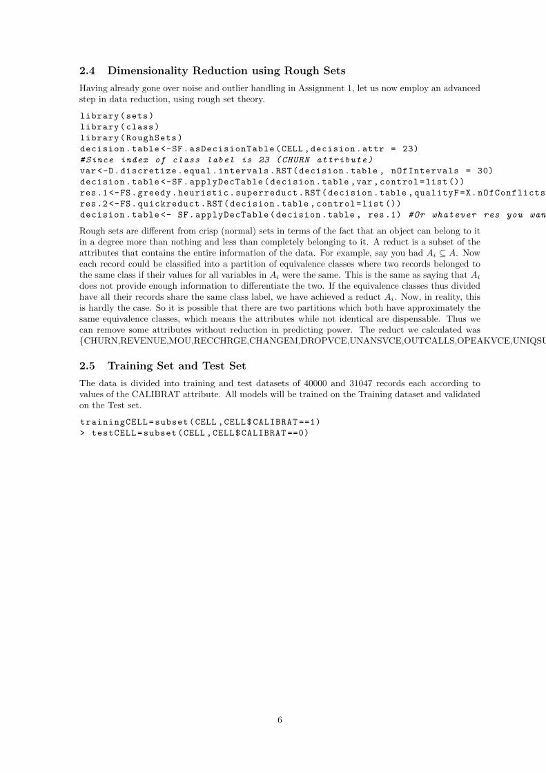
2.4 Dimensionality Reduction using Rough Sets

Having already gone over noise and outlier handling in Assignment 1, let us now employ an advancedstep in data reduction, using rough set theory.

library(sets)

library(class)

library(RoughSets)

decision.table <-SF.asDecisionTable(CELL ,decision.attr = 23)

#Since index of class label is 23 (CHURN attribute)

var <-D.discretize.equal.intervals.RST(decision.table , nOfIntervals = 30)

decision.table <-SF.applyDecTable(decision.table ,var ,control=list ())

res.1<-FS.greedy.heuristic.superreduct.RST(decision.table ,qualityF=X.nOfConflicts)

res.2<-FS.quickreduct.RST(decision.table ,control=list ())

decision.table <- SF.applyDecTable(decision.table , res.1) #Or whatever res you want to choose

Rough sets are different from crisp (normal) sets in terms of the fact that an object can belong to itin a degree more than nothing and less than completely belonging to it. A reduct is a subset of theattributes that contains the entire information of the data. For example, say you had Ai ⊆ A. Noweach record could be classified into a partition of equivalence classes where two records belonged tothe same class if their values for all variables in Ai were the same. This is the same as saying that Ai

does not provide enough information to differentiate the two. If the equivalence classes thus dividedhave all their records share the same class label, we have achieved a reduct Ai. Now, in reality, thisis hardly the case. So it is possible that there are two partitions which both have approximately thesame equivalence classes, which means the attributes while not identical are dispensable. Thus wecan remove some attributes without reduction in predicting power. The reduct we calculated was{CHURN,REVENUE,MOU,RECCHRGE,CHANGEM,DROPVCE,UNANSVCE,OUTCALLS,OPEAKVCE,UNIQSUBS,ACTVSUBS,CSA,MODELS,AGE1,REFURB,CREDITCD,REFER,CREDIT,MARRY}

2.5 Training Set and Test Set

The data is divided into training and test datasets of 40000 and 31047 records each according tovalues of the CALIBRAT attribute. All models will be trained on the Training dataset and validatedon the Test set.

trainingCELL=subset(CELL ,CELL$CALIBRAT ==1)

> testCELL=subset(CELL ,CELL$CALIBRAT ==0)

6

Table 1: Training DatasetActual/Predicted 0 1

0 11488 (TN) 8456 (FP)1 8512 (FN) 11544 (TP)

Table 2: Test DatasetActual/Predicted 0 1

0 17560 (TN) 255 (FP)1 9810 (FN) 354 (TP)

3 Classifiers

Now that we have our data in readily usable format, this section will go through the different classifierswe built to predict churn values.

3.1 Decision Tree

Decision trees conducted from data use condition based nodes to divide the data into smaller subsetshoused at leave nodes classified into the same class. Using the reduct calculated, making a decisiontree of the data becomes a trivial task.

library(party)

tree <-ctree(CHURN~MONTHS+UNIQSUBS+PHONES+RETACCPT ,data=trainingCELL)

print(tree)

plot(tree)

Prediction <-predict(tree ,trainingCELL , type="node")

table(Prediction ,trainingCELL$CHURN)

Prediction <-predict(tree , testCELL , type="node")

table(Prediction , testCELL$CHURN)

The tree was tested on both the training and test data set. The results for both are displayed below:Similiarly, a Decision tree can also be made by the rpart package, generating a subtly different tree

compared to party.

library(rpart)

tree <-part(CHURN~REVENUE+MOU+RECCHRGE+CHANGEM+DROPVCE+UNANSVCE+OUTCALLS+OPEAKVCE+UNIQSUBS+ACTVSUBS+CSA+MODELS+AGE1+REFURB+CREDITCD+REFER+CREDIT+MARRY ,method="class",data=trainingCELL)

printcp(tree)

plot(tree ,uniform=TRUE ,main="Classification Tree for CHURN")

text(tree ,use.n=TRUE ,all=TRUE ,cex =0.8)

pred <-predict(tree ,trainingCELL ,type="class")

table(pred ,trainingCELL$CHURN)

pred <-predict(tree ,testCELL ,type="class")

7

Table 3: Comparing Decision Tree PerformanceTraining (party) Test (party) Training (rpart) Test (rpart)

Accuracy 57.8% 64.2% 55.1% 58%Sensitivity 57.6% 3.5% 55.4% 2.4%Specificity 57.6% 98.6% 54.8% 98.3%

table(pred ,testCELL$CHURN)

8

Table 4: Naive Bayes PerformanceTraining Test

Accuracy 53.98% 57.80%Sensitivity 3.71% 4.28%Specificity 96.43% 97.98%

3.2 Naive Bayes Classifier

A Naive Bayes classifier works on the famous Bayes theorem from probability. The probability of aparticular record belonging to a certain class can be calculated using the probability of having thesame combination of attribute values given a particular class. The naive in the name comes from therather simple approximation that assumes that attributes take values independent of each other.

library(class)

library(e1071)

testCELL$CHURN <-as.factor(testCELL$CHURN)

trainingCELL$CHURN <- as.factor(trainingCELL$CHURN)

model <- naiveBayes(CHURN~REVENUE+MOU+RECCHRGE+CHANGEM+CHANGER+DROPVCE+BLCKVCE+UNANSVCE+MOUREC+OUTCALLS+OPEAKVCE+UNIQSUBS+ACTVSUBS+CSA+MODELS+AGE1+AGE2+CHILDREN+REFURB+TRAVEL+REFER+CREDITAD+CREDIT+MARRY+OCC ,data=trainingCELL)

pred1 <-predict(model , testCELL)

table(pred1 ,testCELL$CHURN)

NBPrediction <- pred1

pred2 <- predict(model , trainingCELL)

table(pred2 , trainingCELL$CHURN)

3.3 Logistic Regression Model

Logistic regression model measures the relationship between the categorical dependent variable andone or more independent variables by estimating probabilities using a logistic function. The model oflogistic regression is based on quite different assumptions from those of linear regression. In particular,the predicted values are probabilities and are therefore restricted to (0,1). A logistic regression modelwas trained to predict the CHURN values.

trainingCELL$CHURN <-as.factor(trainingCELL$CHURN)

model <-glm(CHURN~REVENUE+MOU+RECCHRGE+CHANGEM+DROPVCE+UNANSVCE+OUTCALLS+OPEAKVCE+UNIQSUBS+ACTVSUBS+CSA+MODELS+AGE1+REFURB+CREDITCD+REFER+CREDIT+MARRY ,family="binomial",data=trainingCELL)

trainingCELL$CHURN=as.numeric(trainingCELL$CHURN)

pred <-ifelse(predict(model ,type="response", trainingCELL )>0.5,1,0)

table(pred ,trainingCELL$CHURN)

pred <-ifelse(predict(model ,type="response",testCELL )>0.5,1,0)

table(pred ,testCELL$CHURN)

9

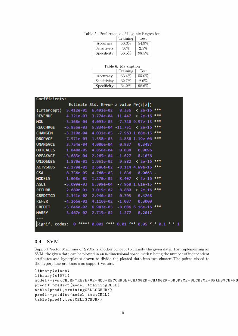
Table 5: Performance of Logistic RegressionTraining Test

Accuracy 56.3% 54.9%Sensitivity 56% 2.5%Specificity 56.5% 98.5%

Table 6: My captionTraining Test

Accuracy 63.4% 55.0%Sensitivity 62.7% 2.6%Specificity 64.2% 98.6%

3.4 SVM

Support Vector Machines or SVMs is another concept to classify the given data. For implementing anSVM, the given data can be plotted in an n-dimensional space, with n being the number of independentattributes and hyperplanes drawn to divide the plotted data into two clusters.The points closed tothe hyperplane are known as support vectors.

library(class)

library(e1071)

model <-svm(CHURN~REVENUE+MOU+RECCHRGE+CHANGEM+CHANGER+DROPVCE+BLCKVCE+UNANSVCE+MOUREC+OUTCALLS+OPEAKVCE+UNIQSUBS+ACTVSUBS+CSA+MODELS+AGE1+AGE2+CHILDREN+REFURB+TRAVEL+REFER+CREDITAD+CREDIT+MARRY+OCC ,data=trainingCELL ,type="C-classification")

pred1 <-predict(model ,trainingCELL)

table(pred1 ,trainingCELL$CHURN)

pred1 <-predict(model ,testCELL)

table(pred1 ,testCELL$CHURN)

10

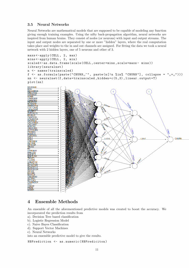
3.5 Neural Networks

Neural Networks are mathematical models that are supposed to be capable of modeling any functiongiving enough training examples. Using the nifty back-propagation algorithm, neural networks areinspired from human brains. They consist of nodes (or neurons) with input and output streams. Theinput and output nodes are separated by one or more ”hidden” layers, where the real computationtakes place and weights to the in and out channels are assigned. For fitting the data we took a neuralnetwork with 2 hidden layers, one of 5 neurons and other of 3.

maxs <-apply(CELL , 2, max)

mins <-apply(CELL , 2, min)

scaled <-as.data.frame(scale(CELL ,center=mins ,scale=maxs - mins))

library(neuralnet)

n <- names(trainscaled)

f <- as.formula(paste("CHURN ~", paste(n[!n %in% "CHURN"], collapse = " + ")))

nn <- neuralnet(f,data=trainscaled ,hidden=c(5,3), linear.output=T)

plot(nn)

4 Ensemble Methods

An ensemble of all the aforementioned predictive models was created to boost the accuracy. Weincorporated the prediction results froma). Decision Tree based classificationb). Logistic Regression Modelc). Naive Bayes Classificationd). Support Vector Machinese). Neural Networksinto an ensemble predictive model to give the results.

NBPrediction <- as.numeric(NBPrediciton)

11

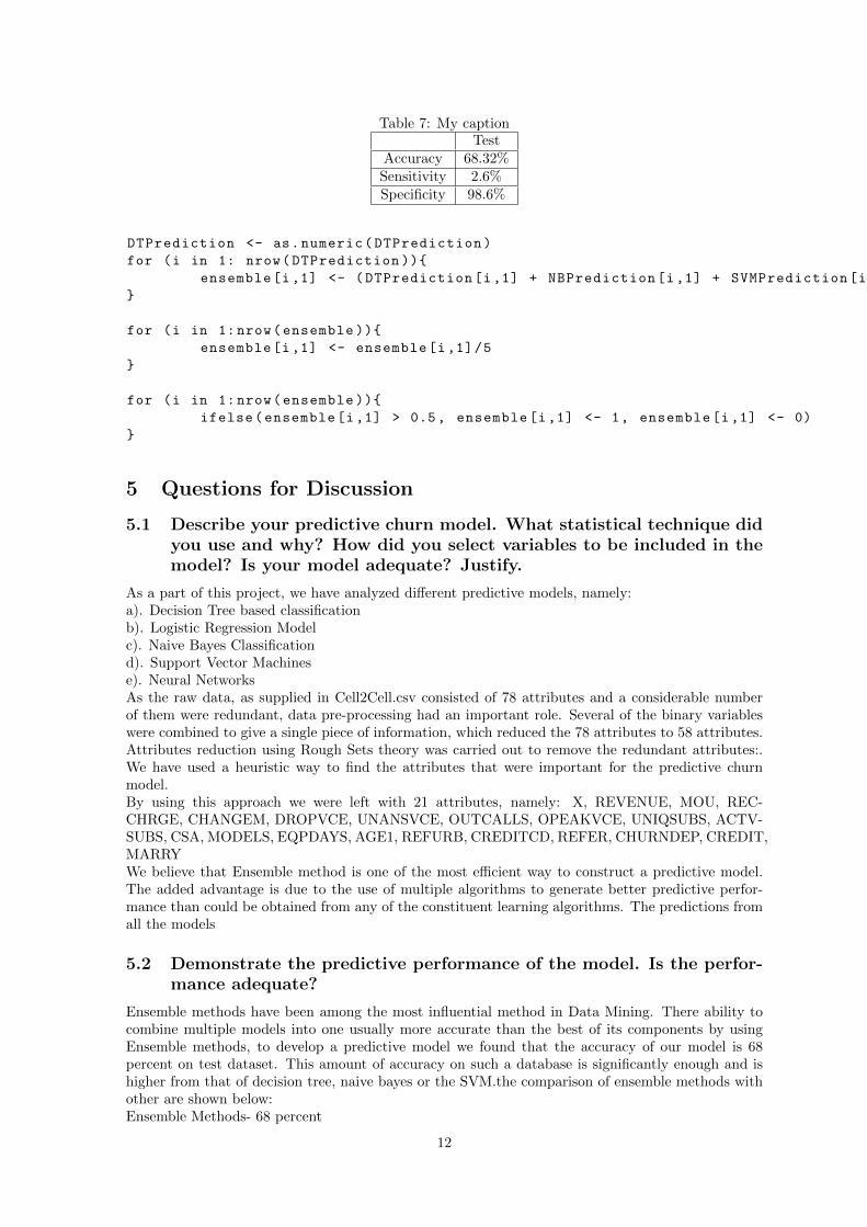
Table 7: My captionTest

Accuracy 68.32%Sensitivity 2.6%Specificity 98.6%

DTPrediction <- as.numeric(DTPrediction)

for (i in 1: nrow(DTPrediction )){

ensemble[i,1] <- (DTPrediction[i,1] + NBPrediction[i,1] + SVMPrediction[i,1] + NNPrediction[i,1] + LRMPredction[i,1])

}

for (i in 1:nrow(ensemble )){

ensemble[i,1] <- ensemble[i,1]/5

}

for (i in 1:nrow(ensemble )){

ifelse(ensemble[i,1] > 0.5, ensemble[i,1] <- 1, ensemble[i,1] <- 0)

}

5 Questions for Discussion

5.1 Describe your predictive churn model. What statistical technique didyou use and why? How did you select variables to be included in themodel? Is your model adequate? Justify.

As a part of this project, we have analyzed different predictive models, namely:a). Decision Tree based classificationb). Logistic Regression Modelc). Naive Bayes Classificationd). Support Vector Machinese). Neural NetworksAs the raw data, as supplied in Cell2Cell.csv consisted of 78 attributes and a considerable numberof them were redundant, data pre-processing had an important role. Several of the binary variableswere combined to give a single piece of information, which reduced the 78 attributes to 58 attributes.Attributes reduction using Rough Sets theory was carried out to remove the redundant attributes:.We have used a heuristic way to find the attributes that were important for the predictive churnmodel.By using this approach we were left with 21 attributes, namely: X, REVENUE, MOU, REC-CHRGE, CHANGEM, DROPVCE, UNANSVCE, OUTCALLS, OPEAKVCE, UNIQSUBS, ACTV-SUBS, CSA, MODELS, EQPDAYS, AGE1, REFURB, CREDITCD, REFER, CHURNDEP, CREDIT,MARRYWe believe that Ensemble method is one of the most efficient way to construct a predictive model.The added advantage is due to the use of multiple algorithms to generate better predictive perfor-mance than could be obtained from any of the constituent learning algorithms. The predictions fromall the models

5.2 Demonstrate the predictive performance of the model. Is the perfor-mance adequate?

Ensemble methods have been among the most influential method in Data Mining. There ability tocombine multiple models into one usually more accurate than the best of its components by usingEnsemble methods, to develop a predictive model we found that the accuracy of our model is 68percent on test dataset. This amount of accuracy on such a database is significantly enough and ishigher from that of decision tree, naive bayes or the SVM.the comparison of ensemble methods withother are shown below:Ensemble Methods- 68 percent

12

Decision tree- 58.85 percentSVM- 54.95 percentNaıve Bayes-57.80 percentLogistic Regression Model- 54.85 percent

5.3 What are the key factors that predict customer churn? Do thesefactors make sense? Why or why not?

By using Logistic regression the relationship between the categorical dependent variable and one ormore independent variables can be established by estimating probabilities using a logistic function.Using Training Data to construct LRM gives following Result:

The following at-tributes are found to be more important in deciding customer churn(High absolute z value and low pvalue) :Revenue,Mean monthly minutes of use,percentage change in minutes of use,Mean no of dropped voicecalls,No of usinq and active subs,Models issued,Age,Refurbished headset,Credit RatingCredit rating , percentage change in minutes of use ,MOU and Mean no of dropped voice calls canbe intuitively understood to be linked to churn as those who cannot afford to pay an increase in billtend to churn to maintain balance .Revenue has a deeper meaning of dependence as “Increased revenue implies more charging on cus-tomers “The other attributes though contribute more to churning of customers as evident from regressioncannot be understood intuitively but as a whole.

13

5.4 What offers should be made to which customers to encourage them toremain with Cell2Cell? Assume that your objective is to generate netpositive cash flow, i.e., generate additional customer revenues aftersubtracting out the cost of the incentive.

The goal is to retain the customer. This should the topmost priority of any company.Here we suggestsome way to reduce the customer churn:

1-One way is is addressing to the customers problem efficiently and effectively. Wireless-telecomindustry involves a list of problem such as slow/down network, billing errors etc. To achieve a goodrelationship with customers one need to keep track of what most customer have asked about. Thesecond thing that a company can use is to develop a system where a customer can know the way thecompany is using to resolve his/her query, the tentative date by which the problem will get fixed andhow to provide the contact details of right person for further inquiry.2- Make use of cross-selling: An important telecom outbound message is the one that gets customersto sign up for an additional product. Surveys have shown that the retention rate of a customer ina telecom industry is a function of the number of products that a customer is buying from yourcompany. For instance,by selling a landline connection to a broadband customer, you make a profitfrom the broadband, but you also reduce the likelihood of churn by this particular customer.

3-The other way is responding wisely to the customers e-mail.The e-mail sent to the customermust be relevant to what the customer might be interested in and just not for the sell purpose.

5.5 Assuming these actions were implemented, how would you determinewhether they had worked?

Loyalty Programs and Technology

Finally, loyalty programs have come a long way since the introduction of the simple punch cardyou handed out to your customers. Today you can manage your program through social media andsmartphone apps, or a customer management system that allows you to track buyer behaviors andconnect with customers through personalized emails or SMS marketing. The data you collect fromyour customer incentive program can also help you to cross promote or up sell additional productsor services and create highly targeted and relevant marketing campaigns to further improve yourbusiness.

14