covid--19: an automatic, semiparametric estimation method ...€¦ · l. fenga covid-19 estimation...

L. Fenga COVID-19 Estimation

CoViD–19: An Automatic,Semiparametric Estimation Methodfor the Population Infected in Italy

Livio FengaItalian National Institute of Statistics

ISTAT, Rome, Italy [email protected]

Abstract: To date, official data on the number of people infectedwith the SARS-CoV-2 - responsible for the CoViD–19 - have been re-leased by the Italian Government just on the basis of a non repre-sentative sample of population which tested positive for the swab.However a reliable estimation of the number of infected, includingasymptomatic people, turns out to be crucial in the preparation ofoperational schemes and to estimate the future number of people,who will require, to different extents, medical attentions. In order toovercome the current data shortcoming, this paper proposes a boot-strap–driven, estimation procedure for the number of people infectedwith the SARS-CoV-2. This method is designed to be robust, auto-matic and suitable to generate estimations at regional level. Obtainedresults show that, while official data at March the 12th report 12.839cases in Italy, people infected wiyh the SARS-CoV-2 could be as highas 105.789.

KEYWORDS: Autoregressive metric; CoViD–19; maximum entropy bootstrap; model un-certainty; number of Italian people infected

1. Introduction

Cases of COVID-19 break out in Italy where it is first attested a capillary spread of thisdisease in the European continent after the Asian one: the scenario that is developing inthese days is creating an example that unfortunately will certainly be repeated in otherstates all over the world. In this framework, the availability of a reliable data sourceson the diffusion of SARS-CoV-2 – the virus responsible for this disease - is crucial inmany ways. It is needed to maximize coordination among emergency services locatedin different parts of the County and within EU, it is crucial for the preparation ofoperational schemes, and pivotal to allow a proper prediction of the development ofthe pandemic.

At the moment, official data on the infection in Italy are based on non random,non representative samples of the population: as a matter of fact people are tested forSARS-CoV-2 on the condition that some symptoms related to the virus are present.These data can ensure a proper estimation of total deaths and total hospitalizationsdue to the virus-related disease: this is crucial to proceed in terms of optimizationavailable resources, of rationalization of accesses to hospitals, of other health facilitiesand so forth. Nonetheless, form a pure statistical point of view they are not suitable toprovide a reliable source of information on the real number of infected people (there-after “positive cases”).

of 14

. CC-BY-NC-ND 4.0 International licenseIt is made available under a is the author/funder, who has granted medRxiv a license to display the preprint in perpetuity. (which was not certified by peer review)

The copyright holder for this preprint this version posted March 18, 2020. .https://doi.org/10.1101/2020.03.14.20036103doi: medRxiv preprint

https://doi.org/10.1101/2020.03.14.20036103

http://creativecommons.org/licenses/by-nc-nd/4.0/


Starting from the number of deaths and the number of people tested positiveto the virus and improving on the methodology originally proposed by Pueyo (2020),this paper aims to estimate the real number of people infected by the SARS-CoV-2,simply called CORONAVIRUS, in each of the 20 Italian regions.

Small sample size – which is suitable to lead to a strong bias in asymptotic re-sults and which is very likely to imply the construction of incorrect confidence intervals– and the distortion of the sample introduced by the mentioned testing strategy are thetwo mayor obstacles in reliable estimations.

The presented procedure is designed to overcome these problems. As it willbe detailed in the sequel, in order to reduce the impact of biasing components on theparameter estimations, a recent bootstrap scheme, called Maximum Entropy Bootstrapand proposed by Vinod et al. (2009), has been employed. In addition to that, a distancemeasure – based on the theory of stochastic processes and proposed by Piccolo (1990)– has been employed to guarantee statistical coherence among all the Italian regions.

2. The proposed method

In small data sets it is essential to save degrees of freedom (DOF). In this perspective,the adopted model — of the type semiparametric – consists of two parts: a purely non-parametric and a parametric one. While the former does not pose problems in termsof DOF, the latter clearly does. However, the sacrifice in terms of DOF is very limitedas an autoregressive model of order 1 (employed in a suitable distance function, asbelow illustrated) has proved sufficient for the purpose. DOF–saving strategy is alsothe driving force of the choice not to consider as an exogenous parameter the georef-erencing of Regions or to include the regional population in a regression–like schemebut to implicitly assumed these variable embedded in the dynamic of the time series inquestion.

3. Data and contageon indicator

The paper makes use of official data published by Italian Authorities, on the followingtwo variables of interest

1. number of deaths from CoViD–19 (denoted by the Latin letter M)

2. number of currently positive cases recorded after the administration of the test(denoted by the Latin letter C).

The data set includes 18 daily datapoints collected at regional level during theperiod of February 24th to March 12th. The total number of Italian regions consideredis 20. However, one special administrative area (Trentino Alto Adige) is divided in twosubregions, i.e. Trento and Bolzano. Therefore, the set containing all the Italian regions– called Ω – has cardinality |Ω| = 22 (the cardinality function is denoted by the symbol| · | = 22). Two different subsets are built from Ω i.e. Ω• – containing the regions forwhich at least one death, out of the group of tested people, has been recorded and Ω

(no recorded deaths):

1. Ω• ≡ Piemonte, Lombardia, V eneto, Friuli, Liguria, Emilia, Toscana,Marche,Lazio,Abbruzzo, V alleAosta,Bolzano,Campania, Puglia, Sicilia

2. Ω ≡ Trento, Umbria,Molise,Basilicata, Calabria, Sardegna,

being Ω ≡ Ω• ∪ Ω. In what follows, the two superscripts • and will bealways used respectively with reference to the regions r1, r2, . . . r15 ∈ Ω• and ins1, s2, . . . s6 ∈ Ω. The time span is denoted as 1, 2, . . . , T.

of 14



https://doi.org/10.1101/2020.03.14.20036103



In the case of the regions included in Ω•, following Pueyo (2020), estimatesthe total number of people infected by CoViD-19 as follows:

y•j,T = p ∗ 2τδ , (1)

wT =CTMT

(2)

where the superscript • identifies the regions r1, r2, . . . r15 ∈ Ω•, w is theratio between current positive cases (C) and number of deaths (M) (2), τ the averagedoubling time for the CoViD–19 (i.e. the average span of time needed for the virusto double the cases) and δ the average time for an infected person to die. These twoconstant terms have been kept fixed as estimated according the data so far availableworldwide (see Pueyo (2020)). They are as follows: τ = 17.3 and δ = 6.2.

The case of the regions belonging to Ω is more complicated. The approachadopted is as follows:

1. Given the sj ∈ Ω a series cπ ∈ Ω• minimizing of a suitable distance function –denoted by the Greek letter π(·) – is found. In symbols: cπ = argmin

(c∈Ω•)

π(s, c);

2. the estimated number of infected at the population level found for cπ, say Icπ

becomes the weight for which the total cases recorded for sj , i.e.Icπ∗CsjCrj

Therefore, the estimate of the variable of interest for this case is as follows:

yj,T =Icπ ∗ CsjCrj

(3)

The distance function adopted (π), called AR distance, has been introduced byPiccolo (2007)). Briefly, the series of interest are considered a realization of an ARMA(Autoregressive Moving Average) model (see, e.g. Makridakis and Hibon (1997)) sothat, each of them can be expressed as an autoregressive model of infinite order, i.e.AR(∞) whose infinite sequence of AR parameters is α1, α2, . . . .

Without loss of generality, the distance between the series s and c π(s, c) (Eqn3) is expressed as

π(s, c) =√

(

∞∑j=1

αj(s)− αj(c)) (4)

4. The Resampling Method

The bootstrap scheme adopted proved to be a real asset for the problem at hand. Giventhe pivotal role played it will be briefly presented. In essence, the choice of the most ap-propriate resampling method is far from being an easy task, especially when the iden-tical and independent distribution iid assumption (Efron’s initial bootstrap method) isviolated. Under dependence structures embedded in the data, simple sampling with re-placement has been proved – see, for example Carlstein et al. (1986) – to yield subopti-mal results. As a matter of fact, iid–based bootstrap schmes are not designed to capture,and therefore replicate, dependence structures. This is especially true under the actualconditions (small sample sizes). In such cases, selecting the “right” resampling schemebecomes a particularly challenging task. Several ad hoc methods have been therefore

of 14



https://doi.org/10.1101/2020.03.14.20036103



proposed, many of which now freely and publicly available in the form of powerful rou-tines working under software package such as Python R© or R R©. In more details, whilein the classic bootstrap an ensemble Ω represents the population of reference the ob-served time series is drawn from, in MEB a large number of ensembles (subsets), sayω1, . . . ,ωN becomes the elements belonging to Ω, each of them containing a largenumber of replicates x1, . . . , xJ. Perhaps, the most important characteristic of theMEB algorithm is that its design guarantees the inference process to satisfy the ergodictheorem. Formally, denoting by the symbol | · | the cardinality function (counting func-tion) of a given ensemble of time series xt ∈ ωi; i = 1, . . . , N, the MEB proceduregenerates a set of disjoint subsets ΩN ≡ ω1 ∩ ω1 · · · ∩ ωN s.t. EΩN ≈ µ(xt), being µ(·)the sample mean. Furthermore, basic shape and probabilistic structure (dependency)is guaranteed to be retained ∀x∗t,j ⊂ ωi ⊂ Ω.

MEB resampling scheme has not negligible advantages over many of the avail-able bootstrap methods: it does not require complicated tune up procedures (unavoid-able, for example, in the case of resampling methods of the type Block Bootstrap) and itis effective under non-stationarity. MEB method relies on the entropy theory and the re-lated concept of (un)informativeness of a system. In particular, the Maximum Entropyof a given density δ(x), is chosen so that the expectation of the Shannon InformationH = E(− log δ(x)), is maximized, i.e.

max(δ)

H = E(− log δ(x)).

Under mass and mean preserving constraints, this resampling scheme gener-ates an ensemble of time series from a density function satisfying (4). Technically, MEBalgorithm can be broken down, following Koutris et al. (2008), in 8 steps. They are:

1. a sorting matrix of dimension T ×2, say S1, accommodates in its first column thetime series of interest xt and an Index Set – i.e. Iind = 2, 3, . . . , T – in the otherone;

2. S1 is sorted according to the numbers placed in the first column. As a result,the order statistics x(t) and the vector Iord of sorted Iind are generated andrespectively placed in the first and second column;

3. compute “intermediate points”, averaging over successive order statistics, i.e.ct =

x(t)+x(t+1)

2 , t = 1, . . . T − 1 and define intervals It constructed on ct and rt,using ad hoc weights obtained by solving the following set of equations:

i)

f(x) =1

r1exp(

[x− c1]

r1); x ∈ I1; r1 =

3x(1)

4+x(2)

4

ii)

f(x) =1

ck − ck−1; x ∈ (ck; ck+1)],

rk =x(k−1)

4+x(k)

2+x(k+1)

4; k = 1, . . . , T − 1;

iii)

f(x) =1

rTexp

([cT−1 − x]

)rT

;x ∈ IT ; rT =xT−1

4+

3xT4

;

of 14



https://doi.org/10.1101/2020.03.14.20036103



4. from a uniform distribution in [0, 1], generate T pseudorandom numbers anddefine the interval Rt = (t/T ; t + 1/T ] for t = 0, 1, . . . , T − 1, in which each pjfalls;

5. create a matching between Rt and It according to the following equations:

xj,t,me = cT−1 − |θ| ln(1− pj) if pj ∈ R0,

xj,t,me = c1 − |θ||ln(1− pj)| if pj ∈ RT−1,

so that a set of T values xj,t, as the jth resample is obtained. Here θ is themean of the standard exponential distribution;

6. a new T × 2 sorting matrix S2 is defined and the T members of the set xj,tfor the jth resample obtained in Step 5 is reordered in an increasing order ofmagnitude and placed in column 1. The sorted Iord values (Step 2) are placed incolumn 2 of S2;

7. matrix S2 is sorted according to the second column so that the order 1, 2, . . . , Tis there restored. The jointly sorted elements of column 1 is denoted by xS,j,t,where S recalls the sorting step;

8. Repeat Steps 1 to 7 a large number of times.

5. The application of the maximum entropy bootstrap

In what follows, the proposed procedure is presented in a step-by-step fashion.

1. For each time series y•t and yt the bootstrap procedure is applied so that B=100 “bona fide” replications are available, i.e. y•t,b; b = 1, 2, . . . B and yt,b; b =1, 2, . . . B;

2. for both the series, the row vector related to the last observation T is extracted,i.e. v = yT,1, y

T,2 . . . y

T,B and v• = y•T,1, y

•T,2 . . . y

•T,B

3. the expected values (E(v•) E(v)) are then extracted as well as the ≈ 95% confi-dence intervals (CI• and CI ), computed according to the t–percentile method.The explanation of the T–percentile method goes beyond the scope of this paper,therefore the interested reader is referred to the excellent paper by Berkowitzand Kilian (2000).

In particular, the lower (upper) CIs will be the lower (upper) bounds of ourestimator while the quantities E(v•) E(v) are estimated through the mean operator,i.e.

µ =6∑j=1

vj (5)

and

µ• =6∑j=1

v•j (6)

At this point, it is worth emphasizing that the procedure not only, as just seen,requires very little in terms of data but can be run in an automatic fashion. Once thedata become available, one has just to divide them according to the subsets Ω i.e. Ω•

of 14



https://doi.org/10.1101/2020.03.14.20036103



and the code will process the new data in an automatic way. The procedure is also veryfast as the computing time needed for the generation of the bootstrap samples requiresless than 2 minutes. Both code and data used for this Paper are freely made availablefor any researcher who would consider using it.

6. Empiricical evidences

In order to give the reader the opportunity to gain a better insight, in Figure 2 – 5the time series of the variable C (see Eqn. 2) is reported for each region. Note thatsudden variations (i.e. Bolzano in Figure 5, Valle D’Aosta in Figure 4 and Molise andCAmpania in Figure 3) are due to the little number of test administrated (denominatorof the variable CT (2))

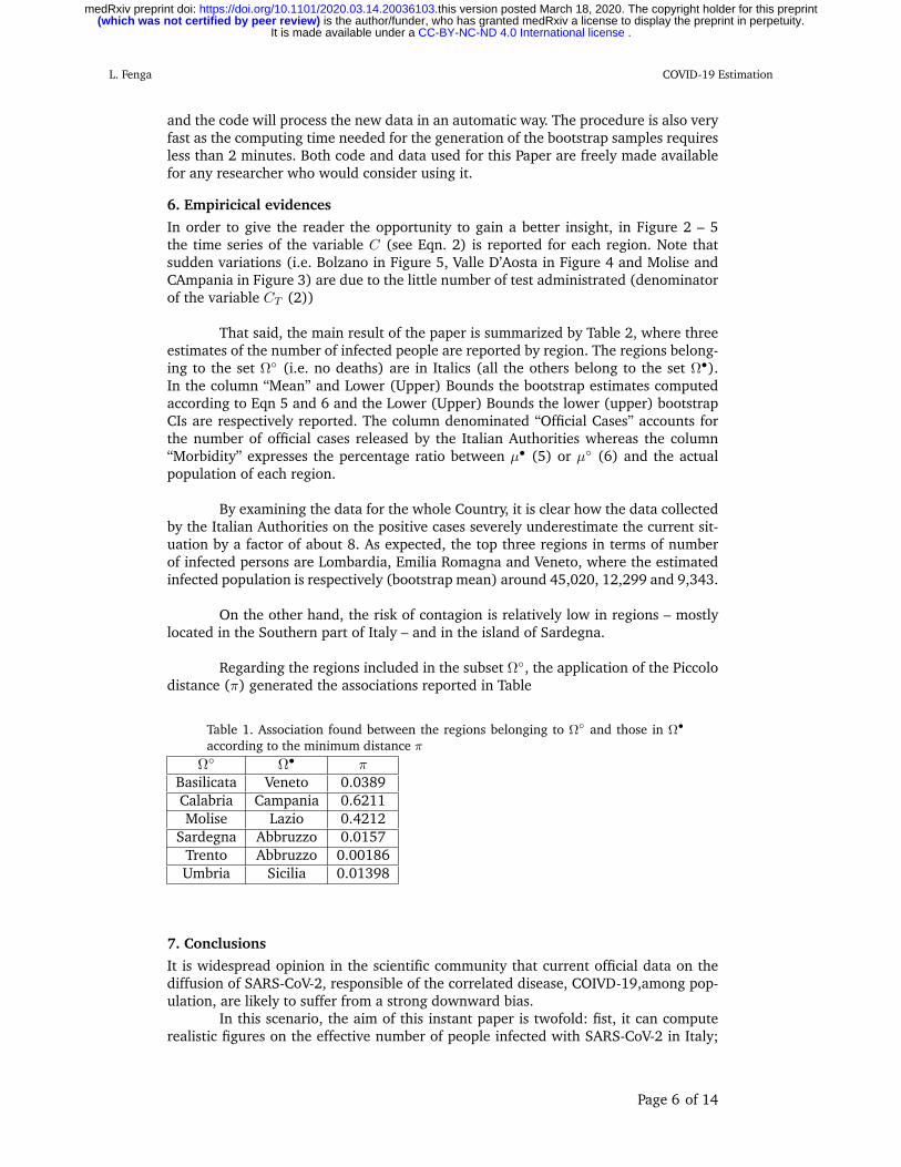
That said, the main result of the paper is summarized by Table 2, where threeestimates of the number of infected people are reported by region. The regions belong-ing to the set Ω (i.e. no deaths) are in Italics (all the others belong to the set Ω•).In the column “Mean” and Lower (Upper) Bounds the bootstrap estimates computedaccording to Eqn 5 and 6 and the Lower (Upper) Bounds the lower (upper) bootstrapCIs are respectively reported. The column denominated “Official Cases” accounts forthe number of official cases released by the Italian Authorities whereas the column“Morbidity” expresses the percentage ratio between µ• (5) or µ (6) and the actualpopulation of each region.

By examining the data for the whole Country, it is clear how the data collectedby the Italian Authorities on the positive cases severely underestimate the current sit-uation by a factor of about 8. As expected, the top three regions in terms of numberof infected persons are Lombardia, Emilia Romagna and Veneto, where the estimatedinfected population is respectively (bootstrap mean) around 45,020, 12,299 and 9,343.

On the other hand, the risk of contagion is relatively low in regions – mostlylocated in the Southern part of Italy – and in the island of Sardegna.

Regarding the regions included in the subset Ω, the application of the Piccolodistance (π) generated the associations reported in Table

Table 1. Association found between the regions belonging to Ω and those in Ω•

according to the minimum distance π

Ω Ω• πBasilicata Veneto 0.0389Calabria Campania 0.6211Molise Lazio 0.4212

Sardegna Abbruzzo 0.0157Trento Abbruzzo 0.00186Umbria Sicilia 0.01398

7. Conclusions

It is widespread opinion in the scientific community that current official data on thediffusion of SARS-CoV-2, responsible of the correlated disease, COIVD-19,among pop-ulation, are likely to suffer from a strong downward bias.

In this scenario, the aim of this instant paper is twofold: fist, it can computerealistic figures on the effective number of people infected with SARS-CoV-2 in Italy;

of 14



https://doi.org/10.1101/2020.03.14.20036103



second, it can provide a methodology, which improves current state of art and can beused to compute similar figures in other countries.

Following Pueyo 2020, this paper proposes a methodology which starts fromItalian data considered restively certain, such as the number of deaths and the numberof people tested positive to the virus, and due to this:

1. allows a population wide estimation of infected people and the computation ofrelated confidence intervals;

2. extends Pueyo 2020 methodology to regions and areas where no deaths havebeen yet registered.

The entire procedure has been written in the programming language R anduses official data as published by the Italian Government. The whole code is madeavailable upon request to any researcher who would consider using it.

Obtained results show that, while official data at March the 12th report 12.839cases in Italy, people infected with the SARS-CoV-2 could be as high as 105.789. If thisestimate were correct, mortality rates would decrease as its denominator increases,compared to what is calculated in official statistics.

On the other hand, considering that, in absence of strong actions, such as thedecreasing of social distance among people and that the average doubling time forthe Coronavirus (that is, the time it takes to double cases, on average) is 6.2 days(Pueyo (2020)), the pandemic is to be regarded as much more dangerous than cur-rently foreseen.To overcome the crisis, international solidarity together wit, strong andcoordinated actions among countries will be crucial. It is even worth to stress that atmicro level everyone is called to act with the greatest responsibility, increasing socialdistance and respecting what imposed by authorities. Stay at home, and, if you can, doresearch on this topic, every contribution could be crucial.

of 14



https://doi.org/10.1101/2020.03.14.20036103



Table 2. Estimation of the number of people infected from CoViD–19 by Italianregions. Lower and Upper Bounds are computed through the Bootstrap t–percentilemethod whereas the mean values is computed as in (5) and (6) In Italics the regionsbelonging to the set Ω are reported

Lower Bound Mean Upper Bound Official Cases Population morbidityAbruzzo 526 600 807 78 1.311.580 0,06Basilicata 48 54 70 8 562.869 0,01Bolzano 697 730 795 103 531.178 0,15Calabria 182 238 493 32 1.947.131 0,03Campania 988 1292 2676 174 5.801.692 0,05Emilia Romagna 10980 12299 14897 1758 4.459.477 0,33Friuli Venezia Giulia 983 1201 2514 148 1.215.220 0,21Lazio 1485 1680 2089 172 5.879.082 0,04Liguria 1346 1608 1995 243 1.550.640 0,13Lombardia 37744 45020 49723 6896 10.060.574 0,49Marche 3151 3891 4593 570 1.525.271 0,30Molise 119 134 167 16 305.617 0,05Piemonte 3216 3703 4217 554 4.356.406 0,10Puglia 490 670 1292 98 4.029.053 0,03Sardegna 244 278 375 39 1.639.591 0,02Sicilia 776 865 1098 111 4.999.891 0,02Toscana 2352 2755 3965 352 3.729.641 0,11Trento 670 764 1028 102 541.098 0,19Umbria 432 481 611 62 882.015 0,07Valle Aosta 139 183 356 26 125.666 0,28Veneto 8382 9343 12028 1297 4.905.854 0,25Totale Italia 74.950 87.789 105.789 12.839 60359546 0,18

of 14



https://doi.org/10.1101/2020.03.14.20036103



Fig. 1. Percentage ratio deaths / new cases for the following Italian regions:Piemonte, Lombardia, Veneto, Liguria and Friuli-Venezia-Giulia

of 14



https://doi.org/10.1101/2020.03.14.20036103



Fig. 2. Percentage ratio deaths / new cases for the following Italian regions Emilia,Toscana, Marche, Lazio and Abruzzo

of 14



https://doi.org/10.1101/2020.03.14.20036103



Fig. 3. Percentage ratio deaths / new cases for the following Italian regions: Molise,Campania, Puglia, Basilicata and Calabria

of 14



https://doi.org/10.1101/2020.03.14.20036103



Fig. 4. Percentage ratio deaths / new cases for the following Italian regions: Sicilia,Valle d’Aosta, Sardegna)

of 14



https://doi.org/10.1101/2020.03.14.20036103



Fig. 5. xxxxxxxxxxxxx

of 14



https://doi.org/10.1101/2020.03.14.20036103



8. Acknowledgments

The author is deeply grateful to Dr. Luigi Di Landro for the generous help in the proof-reading process.

References and linksBerkowitz, J., and Kilian, L. (2000), “Recent developments in bootstrapping time series,” EconometricReviews, 19(1), 1–48.Carlstein, E. et al. (1986), “The use of subseries values for estimating the variance of a general statisticfrom a stationary sequence,” The annals of statistics, 14(3), 1171–1179.Koutris, A., Heracleous, M. S., and Spanos, A. (2008), “Testing for nonstationarity using maximumentropy resampling: A misspecification testing perspective,” Econometric Reviews, 27(4-6), 363–384.Makridakis, S., and Hibon, M. (1997), “ARMA models and the Box–Jenkins methodology,” Journal ofForecasting, 16(3), 147–163.Piccolo, D. (1990), “A distance measure for classifying ARIMA models,” Journal of Time Series Analysis,11(2), 153–164.Piccolo, D. (2007), Statistical issues on the AR metric in time series analysis,, in Proceedings of the SIS2007 intermediate conference” Risk and Prediction, pp. 221–232.Pueyo, T. (2020), Coronavirus: Why You Must Act Now,, in https://medium.com/@tomaspueyo/coronavirus-act-today-or-people-will-die-f4d3d9cd99ca.Vinod, H. D., Lopez-de Lacalle, J. et al. (2009), “Maximum entropy bootstrap for time series: themeboot R package,” Journal of Statistical Software, 29(5), 1–19.

of 14



https://doi.org/10.1101/2020.03.14.20036103


covid--19: an automatic, semiparametric estimation method ...€¦ · l. fenga covid-19 estimation...

Documents