cps 296.3:algorithms in the real world
DESCRIPTION
CPS 296.3:Algorithms in the Real World. Data Compression 4. Compression Outline. Introduction : Lossy vs. Lossless, Benchmarks, … Information Theory : Entropy, etc. Probability Coding : Huffman + Arithmetic Coding Applications of Probability Coding : PPM + others - PowerPoint PPT PresentationTRANSCRIPT
296.3 Page 1
CPS 296.3:Algorithms in the Real World
Data Compression 4
296.3 Page 2
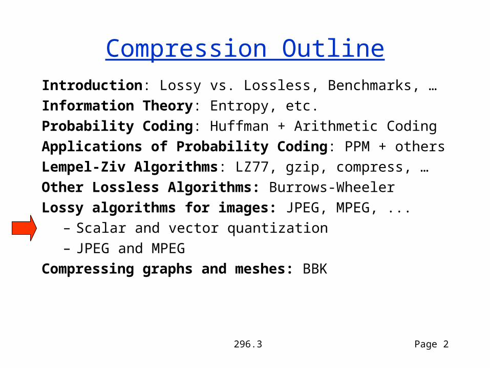
Compression OutlineIntroduction: Lossy vs. Lossless, Benchmarks, …Information Theory: Entropy, etc.Probability Coding: Huffman + Arithmetic CodingApplications of Probability Coding: PPM + othersLempel-Ziv Algorithms: LZ77, gzip, compress, …Other Lossless Algorithms: Burrows-WheelerLossy algorithms for images: JPEG, MPEG, ...
– Scalar and vector quantization– JPEG and MPEG
Compressing graphs and meshes: BBK

296.3 Page 3
Scalar Quantization
Quantize regions of values into a single value:
input
output
uniform
input
output
non uniform
Can be used to reduce # of bits for a pixel

296.3 Page 4
Generate Output
Vector Quantization
Generate Vector
Find closest code vector
Codebook Index Index Codebook
OutIn
Encode Decode

296.3 Page 5
Vector Quantization
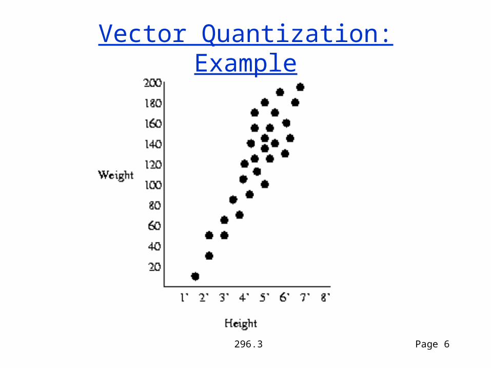
What do we use as vectors?• Color (Red, Green, Blue)
– Can be used, for example to reduce 24bits/pixel to 8bits/pixel
– Used in some terminals to reduce data rate from the CPU (colormaps)
• K consecutive samples in audio• Block of K pixels in an imageHow do we decide on a codebook• Typically done with clustering
296.3 Page 6
Vector Quantization: Example
296.3 Page 7
Linear Transform Coding
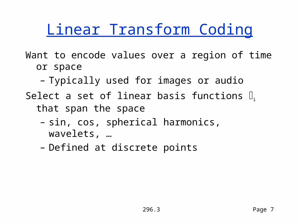
Want to encode values over a region of time or space– Typically used for images or audio
Select a set of linear basis functions i that span the space – sin, cos, spherical harmonics, wavelets, …– Defined at discrete points
296.3 Page 8
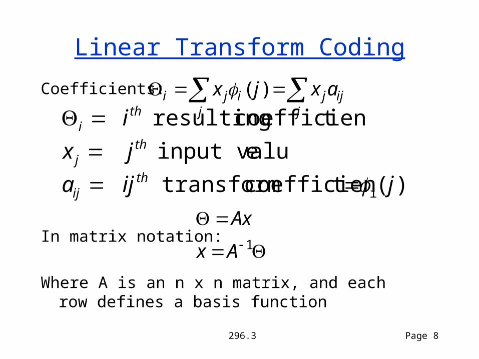
Linear Transform Coding
Coefficients: j
ijjj
iji axjx )(
)( t coefficien transform
einput valu
tcoefficien resulting
i jija
jx
i
thij
thj
thi
In matrix notation:
Where A is an n x n matrix, and each row defines a basis function
1Ax
Ax

296.3 Page 9
Example: Cosine Transform
)(0 j )(1 j
…
xj) i
j
iji jx )(
)(2 j
296.3 Page 10
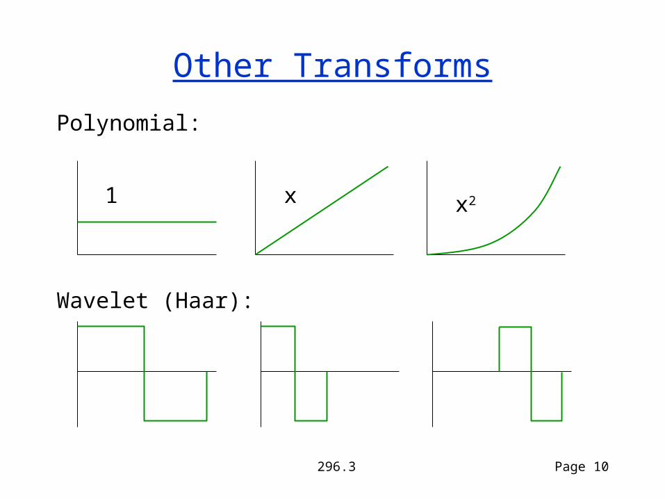
Other Transforms
Polynomial:
1 x x2
Wavelet (Haar):
296.3 Page 11
How to Pick a Transform
Goals:– Decorrelate– Low coefficients for many terms– Basis functions that can be ignored by
perceptionWhy is using a Cosine or Fourier transform
across a whole image bad?How might we fix this?
296.3 Page 12
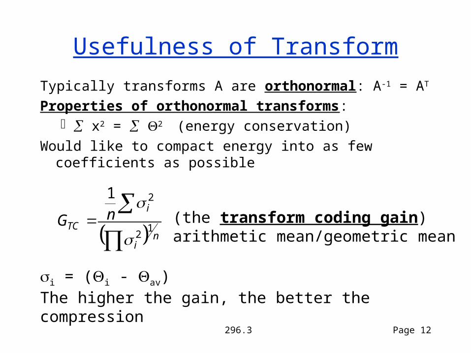
Usefulness of Transform
Typically transforms A are orthonormal: A-1 = AT
Properties of orthonormal transforms: x2 = 2 (energy conservation)
Would like to compact energy into as few coefficients as possible
ni
i
TCnG
12
21
(the transform coding gain)arithmetic mean/geometric mean
i = (i - av)The higher the gain, the better the compression

296.3 Page 13
Case Study: JPEG
A nice example since it uses many techniques:– Transform coding (Cosine transform)– Scalar quantization– Difference coding– Run-length coding– Huffman or arithmetic coding
JPEG (Joint Photographic Experts Group) was designed in 1991 for lossy and lossless compression of color or grayscale images. The lossless version is rarely used.
Can be adjusted for compression ratio (typically 10:1)

296.3 Page 14
JPEG in a Nutshell
(two-dimensional DCT)
Typically down sample I and Q planes by a factor of 2 in each dimension - lossy
296.3 Page 15
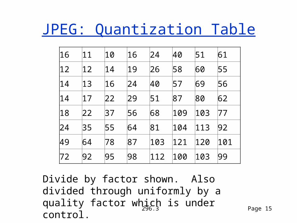
JPEG: Quantization Table
16 11 10 16 24 40 51 61
12 12 14 19 26 58 60 55
14 13 16 24 40 57 69 56
14 17 22 29 51 87 80 62
18 22 37 56 68 109 103 77
24 35 55 64 81 104 113 92
49 64 78 87 103 121 120 101
72 92 95 98 112 100 103 99
Divide by factor shown. Also divided through uniformly by a quality factor which is under control.
296.3 Page 16
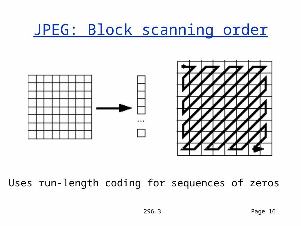
JPEG: Block scanning order
Uses run-length coding for sequences of zeros
296.3 Page 17
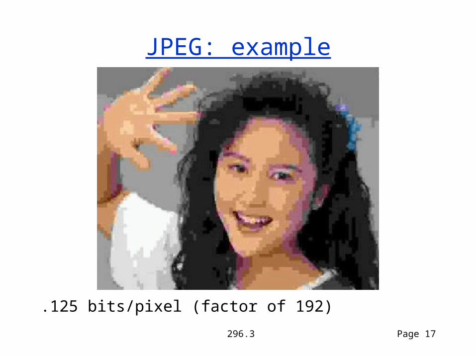
JPEG: example
.125 bits/pixel (factor of 192)
296.3 Page 18
Case Study: MPEG
Pretty much JPEG with interframe codingThree types of frames
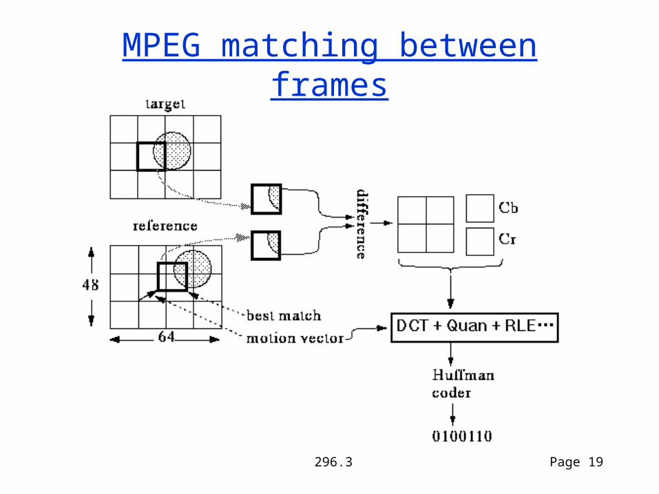
– I = intra frame (aprox. JPEG) anchors– P = predictive coded frames– B = bidirectionally predictive coded frames
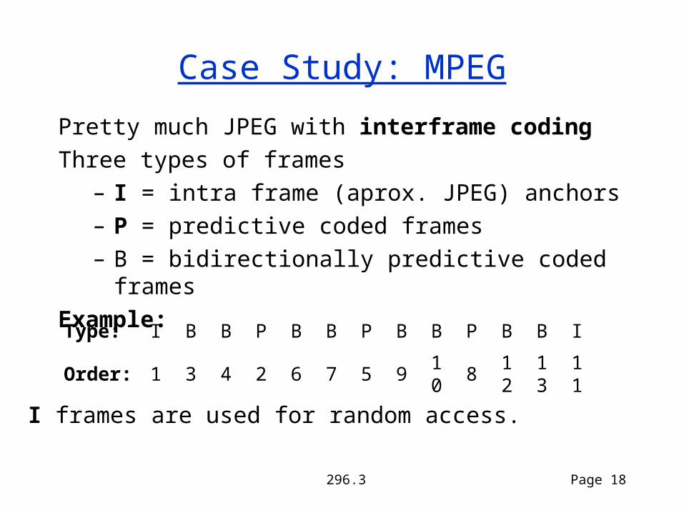
Example:
Type: I B B P B B P B B P B B I
Order: 1 3 4 2 6 7 5 910
812
13
11
I frames are used for random access.
296.3 Page 19
MPEG matching between frames

296.3 Page 20
MPEG: Compression Ratio
30 frames/sec x 4.8KB/frame x 8 bits/byte= 1.2 Mbits/sec + .25 Mbits/sec (stereo audio)
HDTV has 15x more pixels = 18 Mbits/sec
Type Size Compression
I 18KB 7/1
P 6KB 20/1
B 2.5KB 50/1
Average
4.8KB 27/1
356 x 240 image
296.3 Page 21
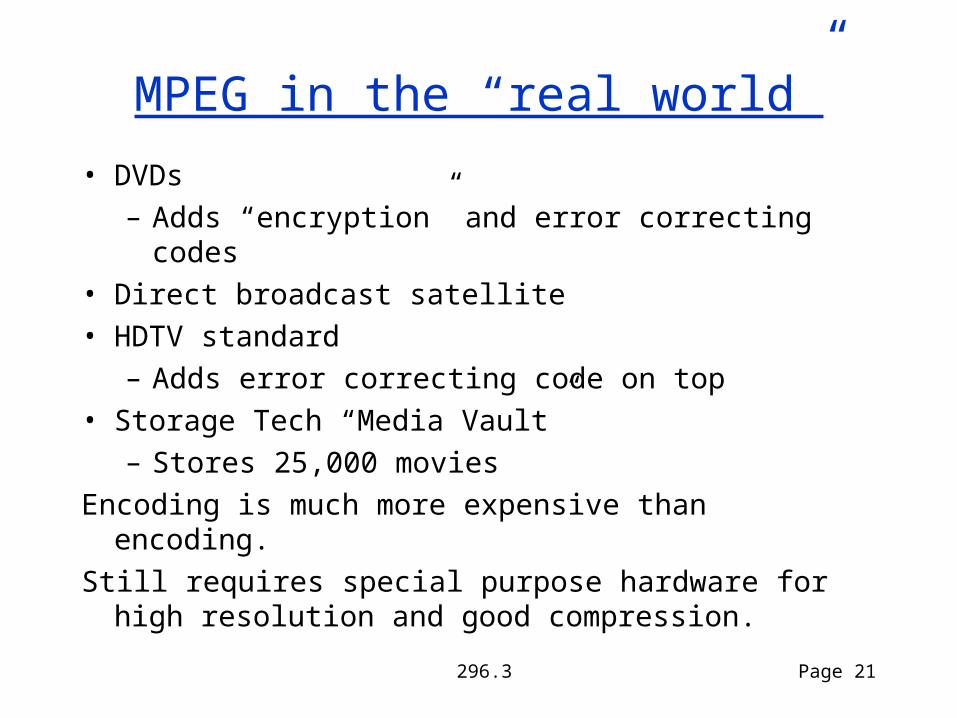
MPEG in the “real world”
• DVDs– Adds “encryption” and error correcting codes
• Direct broadcast satellite• HDTV standard
– Adds error correcting code on top• Storage Tech “Media Vault”
– Stores 25,000 moviesEncoding is much more expensive than encoding.Still requires special purpose hardware for high
resolution and good compression.
296.3 Page 22
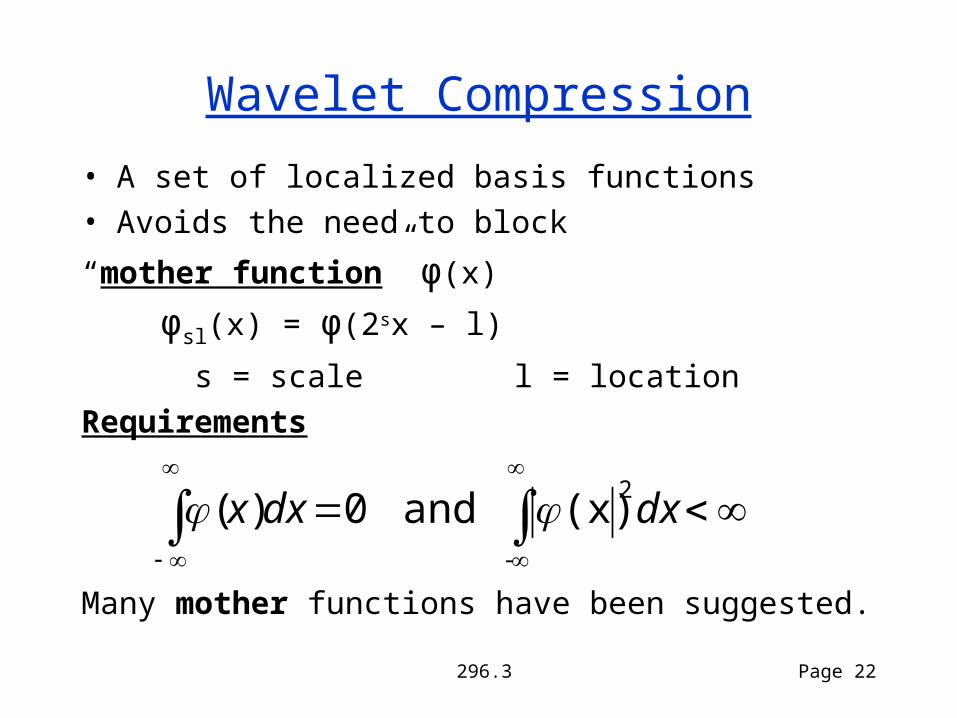
Wavelet Compression
• A set of localized basis functions• Avoids the need to block
“mother function” φ(x)
φsl(x) = φ(2sx – l)
s = scale l = locationRequirements
Many mother functions have been suggested.
-
2(x) and 0)( dxdxx
296.3 Page 23
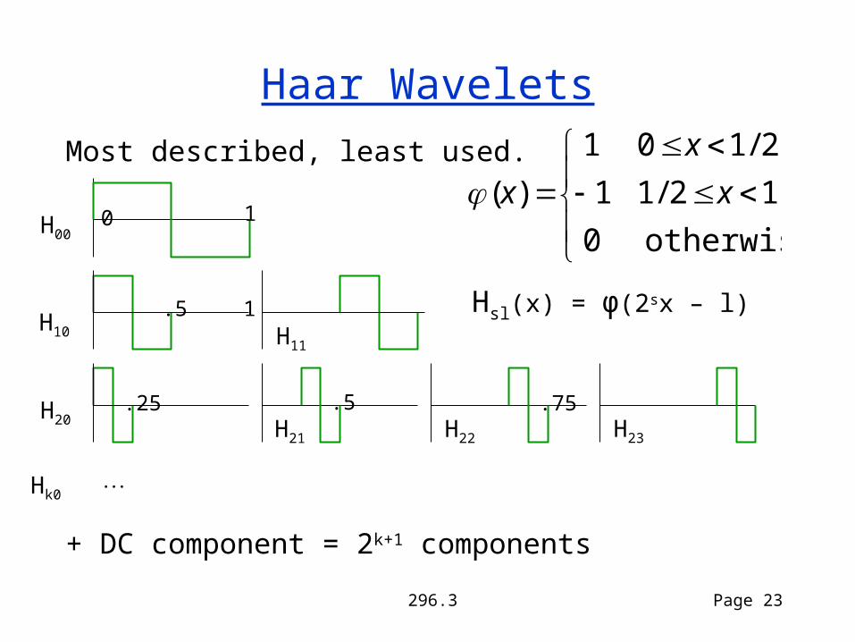
Haar Wavelets
Hsl(x) = φ(2sx – l)
H00
H10
H20 H21 H22 H23
H11
0 1
.5 1
.25 .5 .75
Most described, least used.
otherwise0
12/11
2/101
)( x
x
x
+ DC component = 2k+1 components
Hk0
296.3 Page 24
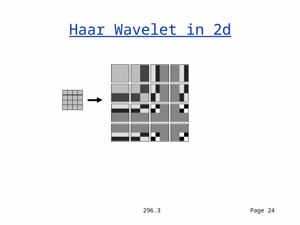
Haar Wavelet in 2d

296.3 Page 25
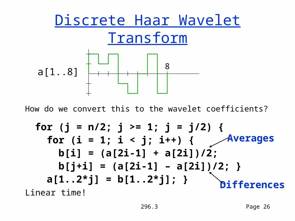
Discrete Haar Wavelet Transform
8
How do we convert this to the wavelet coefficients?
H00
H10
H20 H21 H22 H23
H11
0 1
.5 1
.25 .5 .75
input
296.3 Page 26
Discrete Haar Wavelet Transform
for (j = n/2; j >= 1; j = j/2) { for (i = 1; i < j; i++) { b[i] = (a[2i-1] + a[2i])/2; b[j+i] = (a[2i-1] – a[2i])/2; } a[1..2*j] = b[1..2*j]; }
8
How do we convert this to the wavelet coefficients?
Linear time!
Averages
Differences
a[1..8]
296.3 Page 27
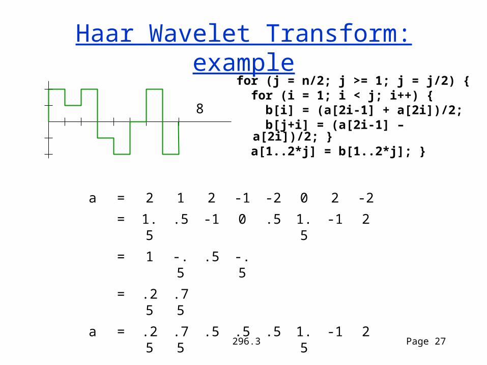
Haar Wavelet Transform: example
8
a = 2 1 2 -1 -2 0 2 -2
= 1.5 .5 -1 0 .5 1.5
-1 2
= 1 -.5 .5 -.5
= .25 .75
a = .25 .75
.5 .5 .5 1.5
-1 2
for (j = n/2; j >= 1; j = j/2) { for (i = 1; i < j; i++) { b[i] = (a[2i-1] + a[2i])/2; b[j+i] = (a[2i-1] – a[2i])/2; } a[1..2*j] = b[1..2*j]; }

296.3 Page 28
Dyadic decomposition
Multiresolution decomposition (e.g., JPEG2000)
1HH1HL
1LH
2LL
2HL 2HH
2LH
296.3 Page 29
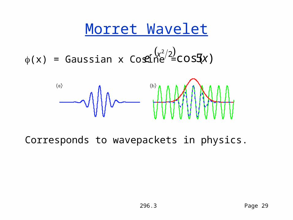
Morret Wavelet
Corresponds to wavepackets in physics.
)5cos(22
xe x(x) = Gaussian x Cosine =

296.3 Page 30
Daubechies Wavelet
296.3 Page 31
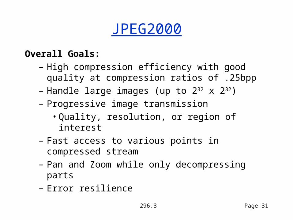
JPEG2000
Overall Goals:– High compression efficiency with good
quality at compression ratios of .25bpp– Handle large images (up to 232 x 232)– Progressive image transmission
• Quality, resolution, or region of interest– Fast access to various points in compressed
stream– Pan and Zoom while only decompressing
parts– Error resilience
296.3 Page 32
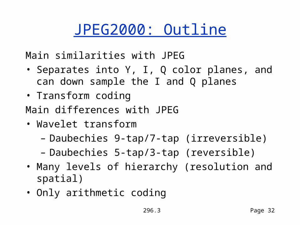
JPEG2000: Outline
Main similarities with JPEG• Separates into Y, I, Q color planes, and can
down sample the I and Q planes• Transform codingMain differences with JPEG• Wavelet transform
– Daubechies 9-tap/7-tap (irreversible)– Daubechies 5-tap/3-tap (reversible)
• Many levels of hierarchy (resolution and spatial)
• Only arithmetic coding
296.3 Page 33
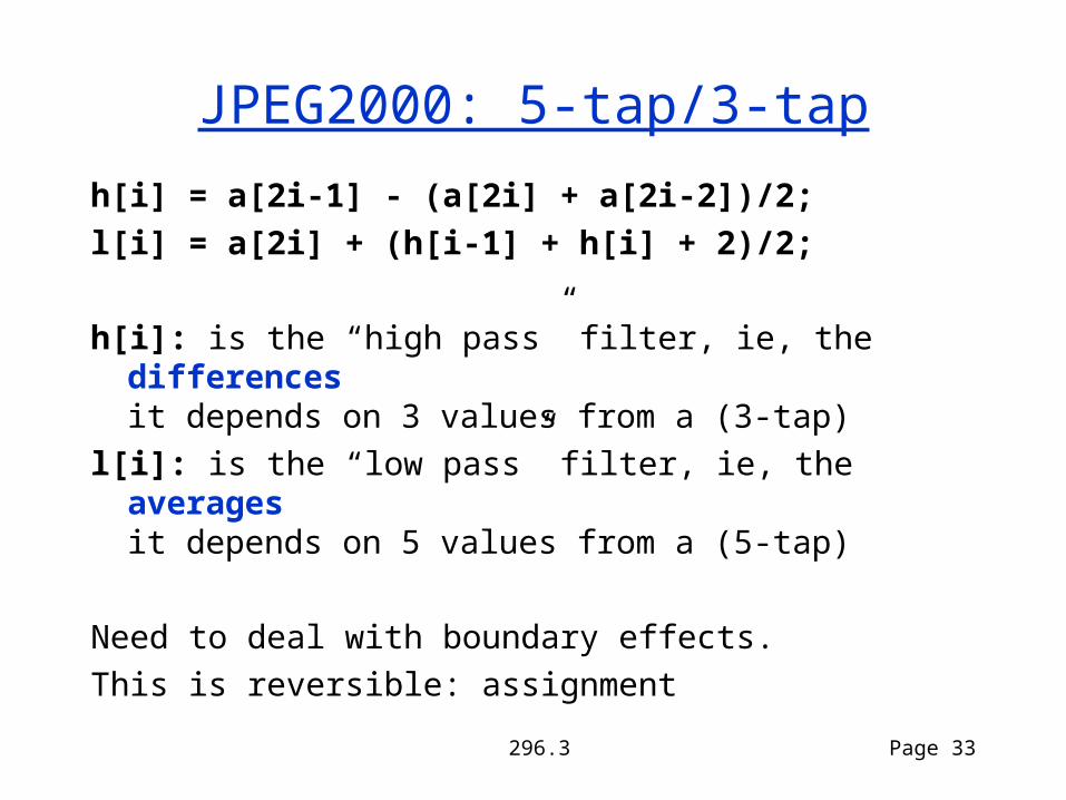
JPEG2000: 5-tap/3-tap
h[i] = a[2i-1] - (a[2i] + a[2i-2])/2;
l[i] = a[2i] + (h[i-1] + h[i] + 2)/2;
h[i]: is the “high pass” filter, ie, the differencesit depends on 3 values from a (3-tap)
l[i]: is the “low pass” filter, ie, the averagesit depends on 5 values from a (5-tap)
Need to deal with boundary effects.This is reversible: assignment

296.3 Page 34
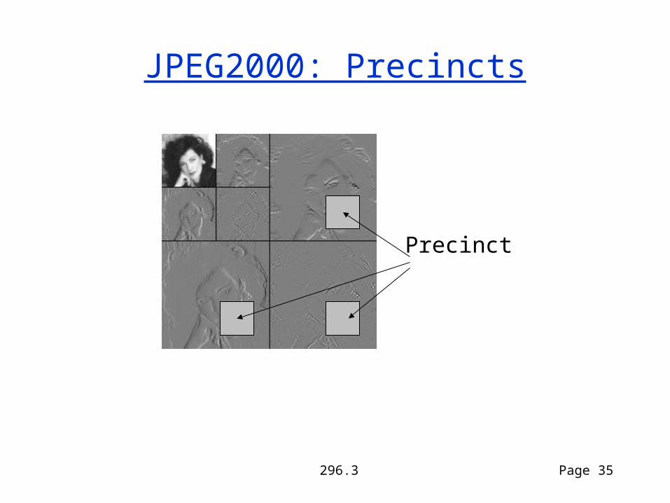
JPEG 2000: Outline
A spatial and resolution hierarchy– Tiles: Makes it easy to decode sections of an
image. For our purposes we can imagine the whole image as one tile.
– Resolution Levels: These are based on the wavelet transform. High-detail vs. Low detail.
– Precinct Partitions: Used within each resolution level to represent a region of space.
– Code Blocks: blocks within a precinct– Bit Planes: ordering of significance of the bits
296.3 Page 35
JPEG2000: Precincts
Precinct

296.3 Page 36
JPEG vs. JPEG2000
JPEG: .125bpp JPEG2000: .125bpp
296.3 Page 37
Compression OutlineIntroduction: Lossy vs. Lossless, Benchmarks,
…Information Theory: Entropy, etc.Probability Coding: Huffman + Arithmetic
CodingApplications of Probability Coding: PPM +
othersLempel-Ziv Algorithms: LZ77, gzip, compress,
…Other Lossless Algorithms: Burrows-WheelerLossy algorithms for images: JPEG, MPEG, ...Compressing graphs and meshes: BBK
296.3 Page 38
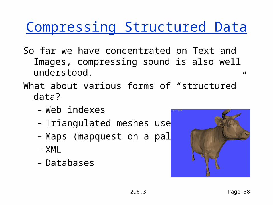
Compressing Structured Data
So far we have concentrated on Text and Images, compressing sound is also well understood.
What about various forms of “structured” data?– Web indexes– Triangulated meshes used in graphics– Maps (mapquest on a palm)– XML– Databases
296.3 Page 39
Compressing Graphs
Goal: To represent large graphs compactly while supporting queries efficiently– e.g., adjacency and neighbor queries– want to do significantly better than
adjacency lists (e.g. a factor of 10 less space, about the same time)
Applications:– Large web graphs – Large meshes– Phone call graphs

296.3 Page 40
How to start?
Lower bound for n vertices and m edges?
1. If there are N possible graphs then we will need log N bits to distinguish them
2. in a directed graph there are n2 possible edges (allowing self edges)
3. we can choose any m of them soN = (n2 choose m)
4. We will need log (n2 choose m) = O(m log (n2/m)) bits in general
For sparse graphs (m = kn) this is hardly any better than adjacency lists (perhaps factor of 2 or 3).
296.3 Page 41
What now?
Are all graphs equally likely?Are there properties that are common across
“real world” graphs?Consider
– link graphs of the web pages– map graphs– router graphs of the internet– meshes used in simulations– circuit graphs
LOCAL CONNECTIONS / SMALL SEPARATORS

296.3 Page 42
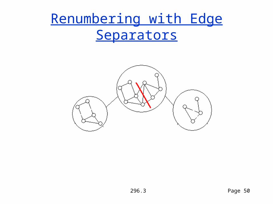
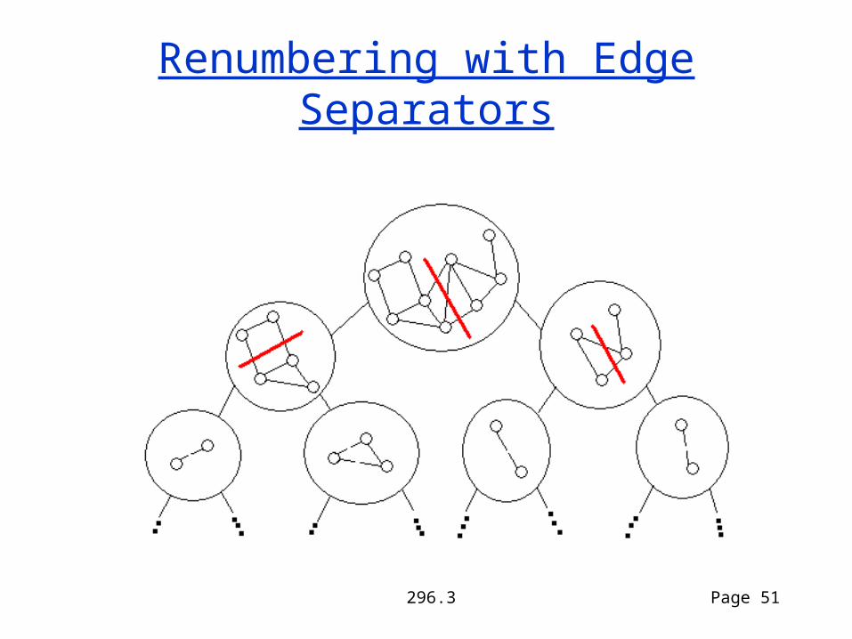
Edge SeparatorsAn edge separator for (V,E) is a
set of edges E’ E whose removal partitions V into two components V1 and V2
Goals:– balanced (|V1| |V2|)– small (|E’| is small)
A class of graphs S satisfies af(n)-edge separator theorem if < 1, > 0 (V,E) S, separator E’, |E’| < f(|V|), |Vi| < |V|, i = 1,2
Can also define vertex separators.
296.3 Page 43
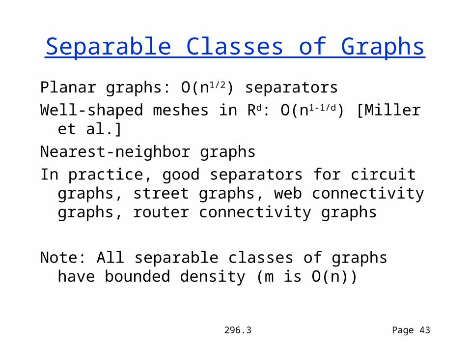
Separable Classes of Graphs
Planar graphs: O(n1/2) separatorsWell-shaped meshes in Rd: O(n1-1/d) [Miller et al.]Nearest-neighbor graphsIn practice, good separators for circuit graphs,
street graphs, web connectivity graphs, router connectivity graphs
Note: All separable classes of graphs have bounded density (m is O(n))
296.3 Page 44
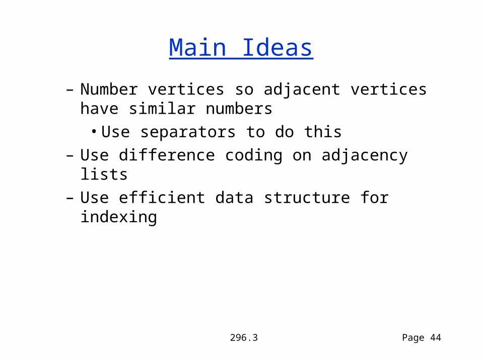
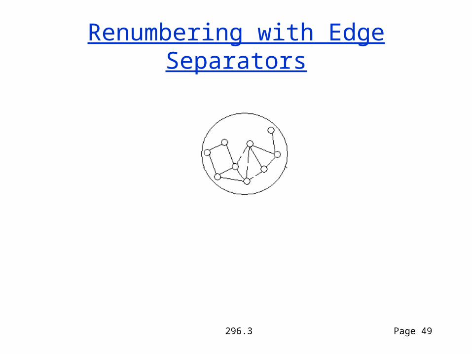
Main Ideas
– Number vertices so adjacent vertices have similar numbers• Use separators to do this
– Use difference coding on adjacency lists– Use efficient data structure for indexing
296.3 Page 45
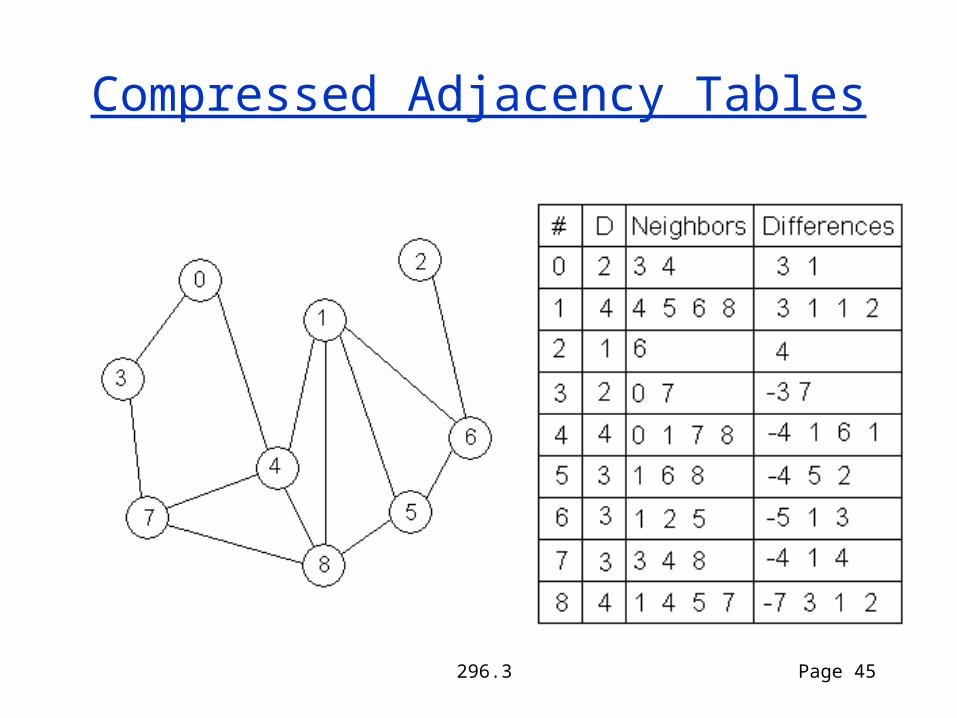
Compressed Adjacency Tables
296.3 Page 46
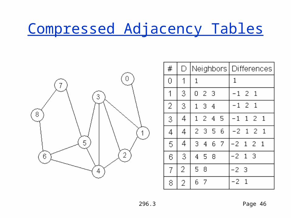
Compressed Adjacency Tables

296.3 Page 47
Log-sized Codes
Log-sized code: Any prefix code that takes O(log(d)) bits to represent an integer d.Gamma code, delta code, skewed Bernoulli code
Example: Gamma codePrefix: unary code for log dSuffix: binary code for d-2log d
(binary code for d, except leading 1 is implied)
296.3 Page 48
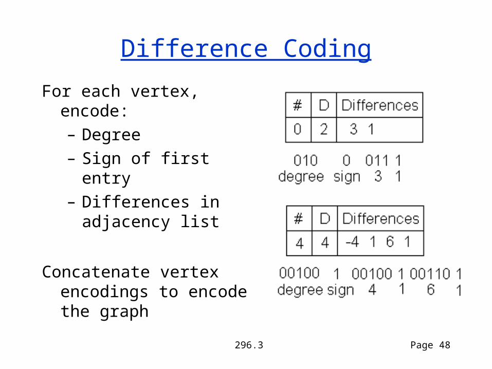
Difference Coding
For each vertex, encode:– Degree– Sign of first entry– Differences in
adjacency list
Concatenate vertex encodings to encode the graph
296.3 Page 49
Renumbering with Edge Separators
296.3 Page 50
Renumbering with Edge Separators
296.3 Page 51
Renumbering with Edge Separators

296.3 Page 52
Renumbering with Edge Separators
296.3 Page 53
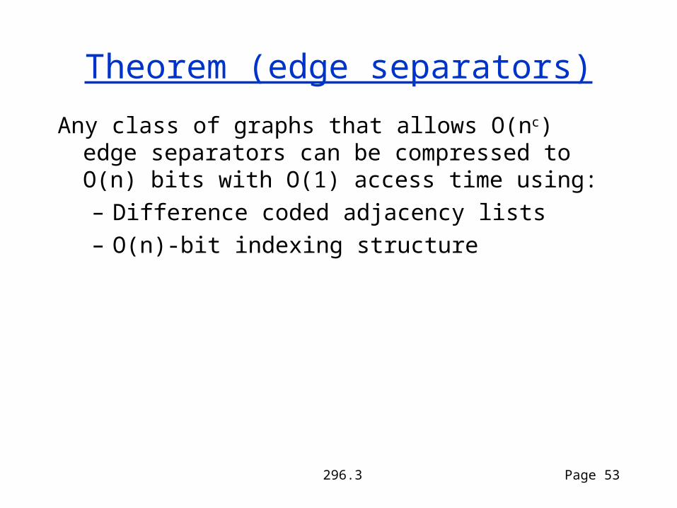
Theorem (edge separators)
Any class of graphs that allows O(nc) edge separators can be compressed to O(n) bits with O(1) access time using:– Difference coded adjacency lists– O(n)-bit indexing structure
296.3 Page 54
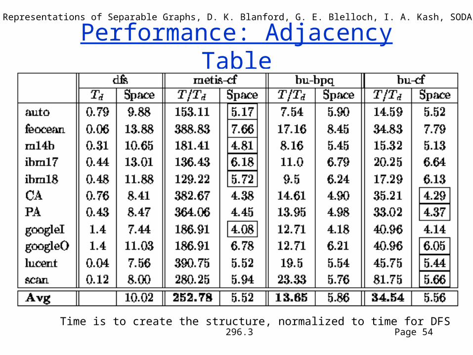
Performance: Adjacency Table
Time is to create the structure, normalized to time for DFS
Compact Representations of Separable Graphs, D. K. Blanford, G. E. Blelloch, I. A. Kash, SODA 2003.
296.3 Page 55
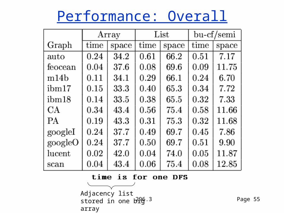
Performance: Overall
Adjacency list stored in one big array
296.3 Page 56
Conclusions
O(n)-bit representation of separable graphs with O(1)-time queries
Space efficient and fast in practice for a wide variety of graphs.
296.3 Page 57
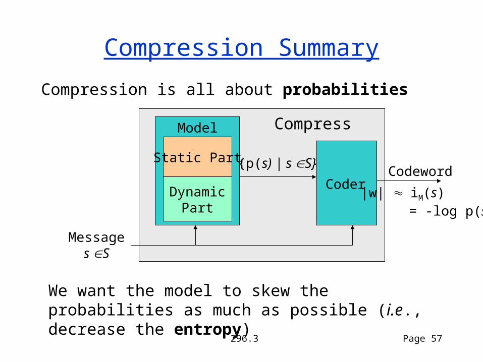
Compression Summary
Compression is all about probabilities
DynamicPart
Static Part
Coder
Messages S
Codeword
Model
{p(s) | s S}
Compress
|w| iM(s) = -log p(s)
We want the model to skew the probabilities as much as possible (i.e., decrease the entropy)
296.3 Page 58
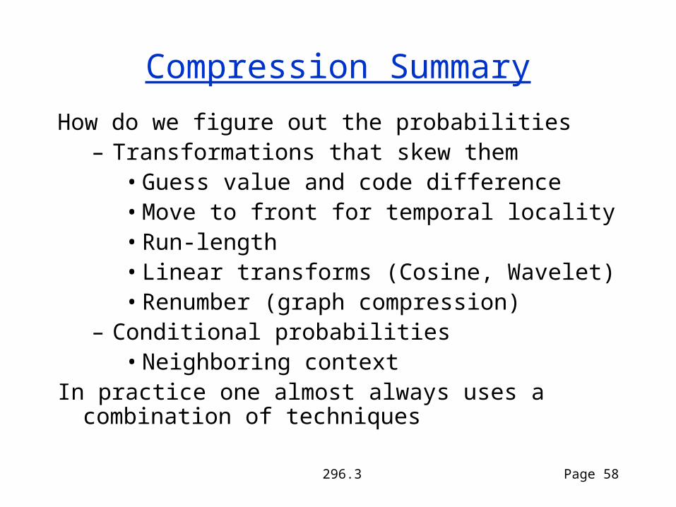
Compression Summary
How do we figure out the probabilities– Transformations that skew them
• Guess value and code difference• Move to front for temporal locality• Run-length• Linear transforms (Cosine, Wavelet)• Renumber (graph compression)
– Conditional probabilities• Neighboring context
In practice one almost always uses a combination of techniques