CPU SCHEDULING

RONG ZHENG

2

OVERVIEW

Why scheduling?

Non-preemptive vs Preemptive policies

FCFS, SJF, Round robin, multilevel queues with feedback, guaranteed scheduling

3

SHORT-TERM, MID-TERM, LONG-TERM SCHEDULER

Long-term scheduler: admission control

Mid-term scheduler: who gets to be loaded in memory

Short-term scheduler: who (in ready queue) gets to be executed

Running Terminated

New Ready Waiting

Admit process

Completion

Interrupt

Get CPU

Exit

System request

SuspendedReady

SuspendedWaiting

Activate Deactivate Deactivate

Completion

SCHEDULING METRICS

Waiting time: Waiting time is the sum of the periods spent waiting in the ready queue.

Turnaround time: The interval from the time of submission of a process to the time of completion is the turnaround time.

• The sum of the periods spent waiting to get into memory, waiting in the ready queue, executing on the CPU, and doing I/O.

Response time (interactive processes): the time from the submission of a request until the first response is produced.

Throughput: number of jobs completed per unit of time

• Throughput related to turningaround time, but not same thing:

5

CRITERIA OF A GOOD SCHEDULING POLICY

Maximize throughput/utilization

Minimize response time, waiting time

• Throughput related to response time, but not same thing

No starvation

• Starvation happens whenever some ready processes never get CPU time

Be fair

• How to measure fairness

Tradeoff exists

6

DIFFERENT TYPES OF POLICIES

A non-preemptive CPU scheduler will never remove the CPU from a running process

• Will wait until the process releases the CPU because i) It issues a system call, or ii) It terminates

• Obsolete

A preemptive CPU scheduler can temporarily return a running process to the ready queue whenever another process requires that CPU in a more urgent fashion

• Has been waiting for too long• Has higher priority

7

JOB EXECUTION

With time slicing, thread may be forced to give up CPU before finishing current CPU burst. Length of slices?

8

FIRST- COME FIRST-SERVED (FCFS)

Simplest and easiest to implement

• Uses a FIFO (First-in-first-out) queue

Previously for non-preemptive scheduling

Example: single cashier grocery store

Process Burst TimeP1 24P2 3P3 3

9

FCFS

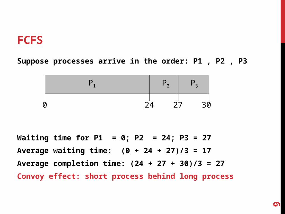
Suppose processes arrive in the order: P1 , P2 , P3

Waiting time for P1 = 0; P2 = 24; P3 = 27

Average waiting time: (0 + 24 + 27)/3 = 17

Average completion time: (24 + 27 + 30)/3 = 27

Convoy effect: short process behind long process

P1 P2 P3

24 27 300

10

FCFS (CONT’D)

Suppose processes arrive in the order: P2, P1 , P3

Waiting time? P1 = 6; P2 = 0; P3 = 3

Average waiting time? 3

Average completion time? (3+6+30)/3 = 13

Good to schedule to shorter jobs first

P1P3P2

63 300

11

SHORTEST JOB FIRST (SJF)

Gives the CPU to the process requesting the least amount of CPU time

• Will reduce average wait• Must know ahead of time how much CPU time each process

needs• Provably achieving shortest waiting time among non-

preemptive policies• Need to know the execution time of processes ahead of time

– not realistic!

12

ROUND ROBIN

All processes have the same priority

Similar to FCFS but processes only get the CPU for a fixed amount of time TCPU

• Time slice or time quantum

Processes that exceed their time slice return to the end of the ready queue

The choice of is TCPU important

• Large FCFS• Small Too much context switch overhead

13

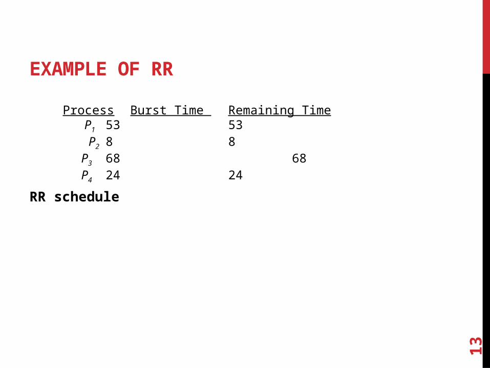
EXAMPLE OF RR

RR schedule

Process Burst Time Remaining Time P1 53 53 P2 8 8P3 68 68P4 24 24

14

EXAMPLE OF RR

RR schedule

Process Burst Time Remaining Time P1 53 33 P2 8 8P3 68 68P4 24 24

P1

0 20

15

EXAMPLE OF RR

RR schedule

Process Burst Time Remaining Time P1 53 33 P2 8 0P3 68 68P4 24 24

P1

0 20

P2

28

16

EXAMPLE OF RR

RR schedule

Process Burst Time Remaining Time P1 53 33 P2 8 0P3 68 48P4 24 24

P1

0 20

P2

28

P3

48

17

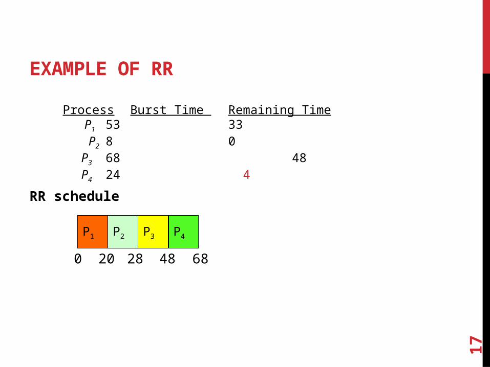
EXAMPLE OF RR

RR schedule

Process Burst Time Remaining Time P1 53 33 P2 8 0P3 68 48P4 24 4

P1

0 20

P2

28

P3

48

P4

68

18

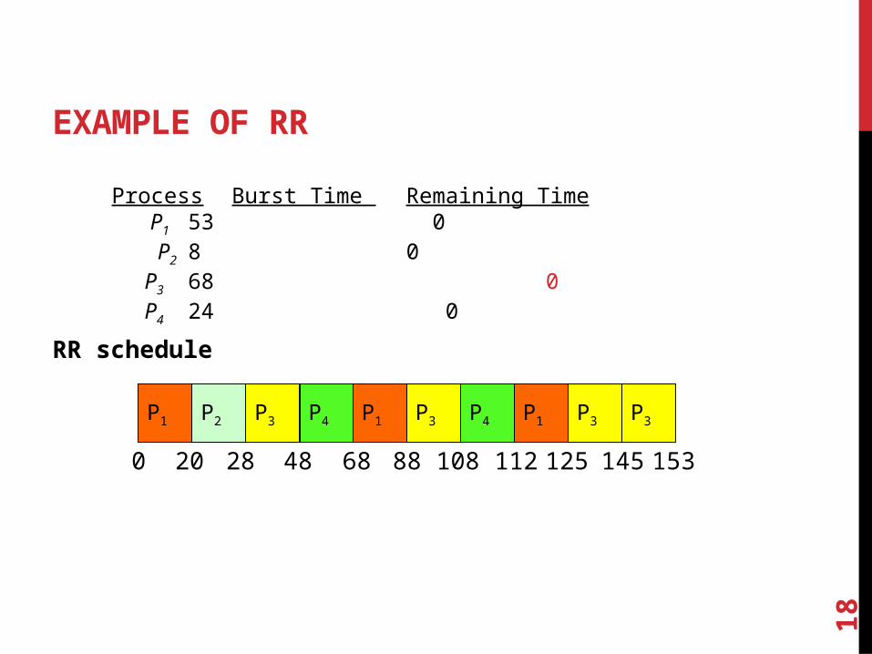
EXAMPLE OF RR

RR schedule

Process Burst Time Remaining Time P1 53 0 P2 8 0P3 68 0P4 24 0

P1

0 20

P2

28

P3

48

P4

68

P1

88

P3

108

P4

112

P1

125

P3

145

P3

153

19

RR WITH QUANTUM = 20

Waiting time for P1=(68-20)+(112-88)=72 P2=(20-0)=20 P3=(28-0)+(88-48)+(125-108)=85 P4=(48-0)+(108-68)=88

Average waiting time = (72+20+85+88)/4=66¼

Average completion time = (125+28+153+112)/4 = 104½

P1

0 20

P2

28

P3

48

P4

68

P1

88

P3

108

P4

112

P1

125

P3

145

P3

153

Quantum

CompletionTime

WaitTime

AverageP4P3P2P1

WITH DIFFERENT TIME QUANTUMP2

[8]P4

[24]P1

[53]P3

[68]

0 8 32 85 153

Best FCFS:

31¼885032Best FCFS

69½32153885Best FCFS

Quantum

CompletionTime

WaitTime

AverageP4P3P2P1

31¼885032Best FCFS

69½32153885Best FCFS

121¾14568153121Worst FCFS

83½121014568Worst FCFS

P2

[8]P4

[24]P1

[53]P3

[68]

0 68 121 145 153

Worst FCFS:

WITH DIFFERENT TIME QUANTUM

Quantum

CompletionTime

WaitTime

AverageP4P3P2P1

6257852284Q = 1

104½11215328125Q = 20

100½8115330137Q = 1

66¼ 88852072Q = 20

31¼885032Best FCFS

121¾14568153121Worst FCFS

69½32153885Best FCFS83½121014568Worst FCFS

95½8015316133Q = 8

57¼5685880Q = 8

99½9215318135Q = 10

99½8215328135Q = 5

61¼68851082Q = 10

61¼58852082Q = 5

P1

0 8 56

P2 P3 P4 P1 P3 P4 P1 P3 P4 P1 P3 P1 P3 P3P3

16 24 32 40 48 64 72 80 88 96 104 112

P1 P3 P1

120 128 133 141 149

P3

153

P2

[8]P4

[24]P1

[53]P3

[68]

0 68 121 145 153

Worst FCFS:

WITH DIFFERENT TIME QUANTUM

23

IN REALITY

The completion time is long with context switches

• More harmful to long jobs

Choice of slices:

• Typical time slice today is between 10ms – 100ms• Typical context-switching overhead is 0.1ms – 1ms• Roughly 1% overhead due to context-switching

P0P2 P3CS CSP1 CS CS P4

24

MULTILEVEL QUEUES WITH PRIORITY

Distinguish among

• Interactive processes – High priority• I/O-bound processes – Medium priority

• Require small amounts of CPU time

• CPU-bound processes – Low priority• Require large amounts of CPU time

(number crunching)

One queue per priority

• Different quantum for each queue

Allow higher priority processes to take CPU away from lower priority processes

1. How do we know which is which?2. What about starvation?

MULTI-LEVEL FEEDBACK SCHEDULING

Use past behavior to predict future

• First used in Cambridge Time Sharing System (CTSS)• Multiple queues, each with a different priority

• Higher priority queues often considered “foreground” tasks

• Each queue has its own scheduling algorithm• e.g., foreground – RR, background – FCFS• Sometimes multiple RR priorities with quantum increasing exponentially

(highest:1ms, next:2ms, next: 4ms, etc.)

Adjust each job’s priority as follows (details vary)

• Job starts in highest priority queue• If timeout expires, drop one level• If timeout doesn’t expire, push up one level (or to top)

Long-Running Compute tasks

demoted to low priority

26

MULTI-PROCESSOR SCHEDULING

Multi-processor on a single machine or on different machines (clusters)

• Process affinity: avoid moving data around• Load balancing• Power consumption

27

SCHEDULING IN LINUX

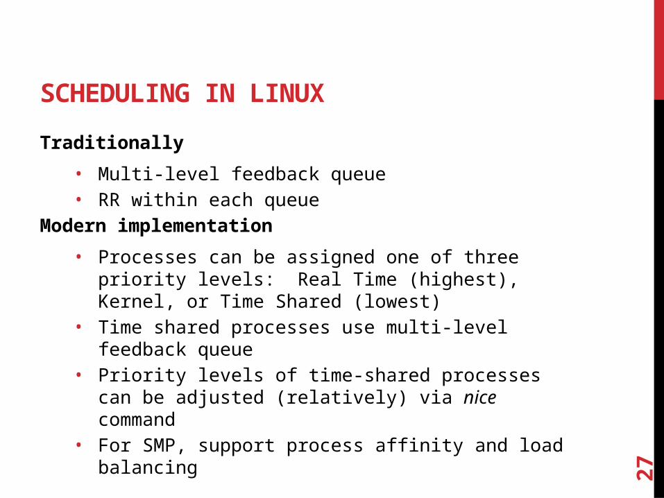
Traditionally

• Multi-level feedback queue• RR within each queue

Modern implementation

• Processes can be assigned one of three priority levels: Real Time (highest), Kernel, or Time Shared (lowest)

• Time shared processes use multi-level feedback queue• Priority levels of time-shared processes can be adjusted

(relatively) via nice command• For SMP, support process affinity and load balancing

28

REAL-TIME SCHEDULING

29

REAL-TIME SYSTEMS

Systems whose correctness depends on their temporal aspects as well as their functional aspects

• Control systems, automotive …

Performance measure

• Timeliness on timing constraints (deadlines)• Speed/average case performance are less significant.

Key property

• Predictability on timing constraints

Hard vs soft real-time systems

30

REAL-TIME WORKLOAD

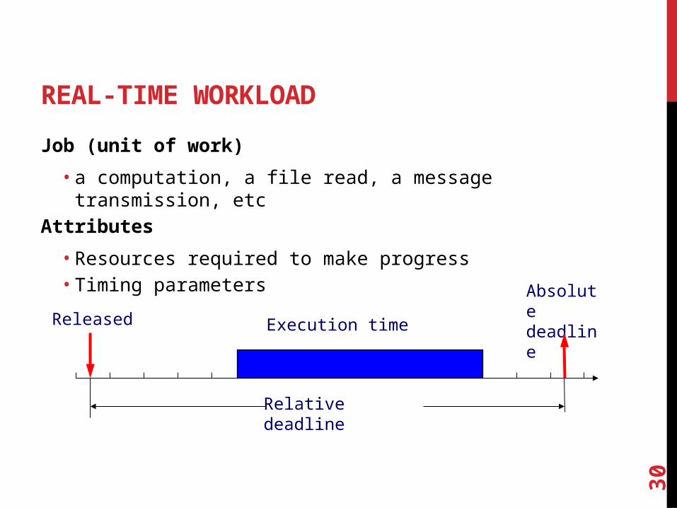
Job (unit of work)

• a computation, a file read, a message transmission, etc

Attributes

• Resources required to make progress• Timing parameters

Released

Absolute deadline

Relative deadline

Execution time

31

REAL-TIME TASK

Task : a sequence of similar jobs

• Periodic task (p,e)• Its jobs repeat regularly• Period p = inter-release time (0 < p)• Execution time e = maximum execution time (0 < e < p)• Utilization U = e/p

5 10

150

32

RATE MONOTONIC

Optimal static-priority scheduling

It assigns priority according to period

A task with a shorter period has a higher priority

Executes a job with the shortest period

(4,1)

(5,2)

(7,2)

5

5

10

10 15

15

T1

T2

T3

33

RM (RATE MONOTONIC)

Executes a job with the shortest period

(4,1)

(5,2)

(7,2)

5

5

10

10 15

15

T1

T2

T3

34

RM (RATE MONOTONIC)

Executes a job with the shortest period

(4,1)

(5,2)

(7,2)

Deadline Miss !

5

5

10

10 15

15

T1

T2

T3

RM Utilization Bounds

0.5

0.6

0.7

0.8

0.9

1

1.1

1 4 16 64 256 1024 4096

The Number of Tasks

Util

izat

ion

RM – UTILIZATION BOUND

Real-time system is schedulable under RM if

∑Ci/Ti ≤ n (21/n-1)

Ci is the computation time (work load), Ti is the period

36

EDF (EARLIEST DEADLINE FIRST)

Optimal dynamic priority scheduling

A task with a shorter deadline has a higher priority

Executes a job with the earliest deadline

(4,1)

(5,2)

(7,2)

5

5

10

10 15

15

T1

T2

T3

37

EDF (EARLIEST DEADLINE FIRST)

Executes a job with the earliest deadline

(4,1)

(5,2)

(7,2)

5

5

10

10 15

15

T1

T2

T3

38

EDF (EARLIEST DEADLINE FIRST)

Executes a job with the earliest deadline

(4,1)

(5,2)

(7,2)

5

5

10

10 15

15

T1

T2

T3

39

EDF (EARLIEST DEADLINE FIRST)

Executes a job with the earliest deadline

(4,1)

(5,2)

(7,2)

5

5

10

10 15

15

T1

T2

T3

40

EDF (EARLIEST DEADLINE FIRST)

Optimal scheduling algorithm

• if there is a schedule for a set of real-time tasks,

EDF can schedule it.

(4,1)

(5,2)

(7,2)

5

5

10

10 15

15

T1

T2

T3

41

EDF – UTILIZATION BOUND

Real-time system is schedulable under EDF if and only if

∑Ci/Ti ≤ 1

Liu & Layland,

“Scheduling algorithms for multi-programming in a hard-real-time environment”, Journal of ACM, 1973.

42

SUMMARY

Scheduling matters when resource is tight

• CPU, I/O, network bandwidth• Preemptive vs non-preemptive• Burst time known or unknown• Hard vs soft real-time• Typically tradeoff in fairness, utilization

and real-timelinessUtilization

Resp

on

se time

100%

43

COMPARISONUtilization (throughput)

Response time Fairness

FCFS 100% High Good

SJF 100% Shortest Poor

RR 100% Medium Good

Multi-level priority with feedback

100% Short Good

RM ∑Ci/Ti ≤ n (21/n-1) - -

EDF 100% - -