crack detection inside pipelines using mechatronics … · 2 crack detection inside pipelines using...
TRANSCRIPT
1
School of Science and Engineering
University Honors Program
CRACK DETECTION INSIDE PIPELINES
USING MECHATRONICS AND COMPUTER
VISION
Afaf Remani
Dr. Hassan Darhmaoui, Dr. Naeem Nisar Sheikh
Spring 2018

2
CRACK DETECTION INSIDE PIPELINES USING
MECHATRONICS AND COMPUTER VISION
Honors Capstone Report
I, Afaf Remani, hereby affirm that I have applied ethics to the design process and in the
selection of the final proposed design. And that I have held the safety of the public to be
paramount and have addressed this in the presented design wherever may be applicable.
Approved by both supervisors

3
Acknowledgements
It is with great pleasure that I would like to express my gratitude to the people who
significantly helped me throughout this journey, and whose valuable assistance has brought
this project to be. First and foremost, I would like to present my warmest thanks to my
supervisors Dr. Hassan Darhamoui and Dr. Naeem Nisar Sheikh for their continuous
assistance, solid support, as well as dedicated involvement all along the different phases of
this project.
This project is the offspring of several efforts combined, among which my family’s
assistance was the most significant. I would like to cease this opportunity to extend the
thanks to my little family, namely my parents and my siblings, who were supportive of me
throughout my journey at Al Akhawayn, and helped me finance this project and order the
necessary hardware to build my system. The realization of the final physical prototype would
not have been possible without them.
It is also my pleasure to thank my friends who have been continuously supportive of
me, cheered me throughout this project, and were always excited to hear about my
advancements, notably my friend Mohammed El Kihal who assisted me during the tedious
installation of OpenCV on Raspbian Stretch, which took a couple of days. Additionally, I
would like to thank the department of Ground and Maintenance at Al Akhawayn University,
notably Mr. Mohamed Zaki, who has provided me with valuable information, and given me
the opportunity to test my system inside real industrial pipes.
Last but not least, I would like to present utmost gratitude to the School of Science
and Engineering and Mr. Najem Naji, for granting me access to the Linux laboratory to
perform my image processing testing. Warm thanks also go to the Honors Program for this
great opportunity to work on an Honors capstone, as well as for the academic assistance and
background I was offered during these past four years.
This project would not have come to life hadn’t it been for the valuable help and
assistance of said parties, and is representative of an amazing and instructive journey at Al
Akhawayn University.
4
Table of Contents
Acknowledgements .................................................................................................................... 3
List of Figures ............................................................................................................................ 7
List of Tables ............................................................................................................................. 9
Abstract .................................................................................................................................... 10
1. INTRODUCTION ........................................................................................................... 11
1.1 Context and Motivation ....................................................................................................... 11
1.2 Methodology and Objectives ............................................................................................... 11
2. LITERATURE REVIEW ................................................................................................ 13
2.1 Existing Technologies for Crack Detection ................................................................................ 13
2.1.1 Industrial Ultrasonic Testing ............................................................................................... 13
2.1.2 Microwave Imaging Technique........................................................................................... 15
2.1.3 Liquid Penetrant Testing ..................................................................................................... 18
2.1.4 Image Processing Technique ............................................................................................... 21
2.2. Theoretical Background ................................................................................................ 22
2.2.1 Introduction to Contemporary Robotics .............................................................................. 22
2.2.2 Mobile Platforms ................................................................................................................. 24
2.2.3 Introduction to Image Processing ........................................................................................ 25
3. HARDWARE ARCHITECTURE AND ASSEMBLY ................................................... 28
3.1 Hardware Components ........................................................................................................ 28
3.2 Internal Functional Architecture .......................................................................................... 29
3.3 Mounting and Assembly ...................................................................................................... 31
4. COMPUTER-AIDED DESIGN OF THE ROBOT’S HOUSING .................................. 33
4.1 Modeling the Sensors’ Housing - Alternative #1 ................................................................ 33
4.2 Modeling the Sensors’ Housing - Alternative #2 ................................................................ 35
5. KINEMATICS AND MOTION STUDY ........................................................................ 37
5.1 Basics and Assumptions ...................................................................................................... 37
5.1.1 Differential Drive Kinematics ......................................................................................... 37
5.1.2 Forward Kinematics ........................................................................................................ 39
5.2 Displacement and Positioning ............................................................................................. 39
5.3 Motion and Kinematics’ Algorithm .................................................................................... 41
5
6. PLATFORM CONTROL ................................................................................................ 44
6.1 Control Theory .................................................................................................................... 44
6.2 Control Method – PID Controller ........................................................................................ 45
6.2.1 PID Controller’s Coefficients .......................................................................................... 45
6.2.2 PID Algorithm ................................................................................................................. 47
7. POSITION TRACKING USING EXTERNAL SENSORS ............................................ 49
7.1 Rotary Encoders .................................................................................................................. 49
7.2 Ultrasonic Sensors ............................................................................................................... 50
7.2.1 Concept and Operation .................................................................................................... 50
7.3 Infrared Sensor .................................................................................................................... 51
7.3.1 Concept and Operation .................................................................................................... 51
7.3.2 Experimentation and Curve Fitting ................................................................................. 53
7.4 Light-Emitting Diodes (LEDs) ............................................................................................ 54
7.5 Sensors’ Arduino Code – Overall Summary ....................................................................... 55
8. RASPBERRY PI SET-UP AND SOFTWARE MANAGEMENT ................................. 56
8.1 Board Set-Up ....................................................................................................................... 56
8.2 Software Management ......................................................................................................... 57
8.2.1 Raspbian Stretch Installation ........................................................................................... 57
8.2.2 Python PiCamera Configuration ..................................................................................... 58
9. REAL-TIME COMPUTER VISION AND IMAGE PROCESSING ............................. 63
9.1 Installing OpenCV and Python 3 on Raspbian Stretch ............................................................... 63
9.2 Image Processing for Crack Detection ................................................................................ 67
9.2.1 Image Capturing .............................................................................................................. 67
9.2.2 Image Processing Using OpenCV ................................................................................... 68
10. RESULTS AND TESTING ......................................................................................... 78
10.1 Motion and Sensors’ Testing .................................................................................................... 78
10.2 The Image Processing Test .................................................................................................. 80
11. FINANCIAL ANALYSIS AND MONETARY INVESTMENTS ............................. 82
11.1 Itemization of the Project’s Tangible Costs .............................................................................. 82
11.2 Itemization of the Project’s Intangible Costs ....................................................................... 83
11.3 Expenditure Optimization and Weighted Decision Matrix ................................................. 84
11.4 Global Monetary Investment and Budget Division ............................................................. 85
12. CRACK DETECTION IN MOROCCO – INTERVIEWS ......................................... 88

6
12.1 Crack Detection Methods at Al Akhawayn University’s Ground and Maintenance
Department, Ifrane ............................................................................................................................ 88
12.2 Crack Detection Methods at RADEEMA, Marrakech ........................................................ 90
13. SYSTEM ADVANTAGES AND LIMITATIONS ..................................................... 93
13.1 System Advantages ................................................................................................................... 93
13.2 System Limitations ................................................................................................................... 93
14. HONORS PROGRAM REQUIREMENT ................................................................... 94
14.1 Environmental Impact .............................................................................................................. 94
14.2 Ethical Considerations .............................................................................................................. 94
14.3 Research and Multidisciplinarity .............................................................................................. 94
15. STEEPLE Analysis ...................................................................................................... 96
16. CONCLUSION AND FUTURE WORK .................................................................... 99
17. BIBLIOGRAPHY ...................................................................................................... 101
Appendix A – Motion and Control, Arduino Code ............................................................... 105
Appendix B – Crack Detection, Python Code ....................................................................... 110
Appendix C – Image Capture, Python Code .......................................................................... 112
Appendix D – Raspberry Pi V2 HD Camera, Datasheet ....................................................... 113

7
List of Figures
Figure 1: Reflection and refraction of sound wave beams [2] ................................................. 14
Figure 2: Crack inspection’s functional principle [2] .............................................................. 15
Figure 3: Sound waves’ amplitude versus time-of-flight [2] ................................................... 15
Figure 4: “Side view of a surface crack and an open-ended rectangular waveguide aperture”
[4] ..................................................................................................................................... 17
Figure 5: “Front view of a surface crack and an open-ended rectangular waveguide aperture”
[4] ..................................................................................................................................... 18
Figure 6: The liquid penetrant’s visible spotting on a concrete surface, indicating a crack [5]
.......................................................................................................................................... 18
Figure 7: Illustration of the larger dye covered surface compared to the flaw [5] .................. 19
Figure 8: A penetrant being allowed dwell time [5] ................................................................ 20
Figure 9: Illustration of excess penetrant removal [5] ............................................................. 20
Figure 10: Illustration of the indication development phase [5] .............................................. 21
Figure 11: Cycle diagram of contemporary robotics ............................................................... 23
Figure 12: Modern robots’ main functionalities ...................................................................... 24
Figure 13: A wheeled mobile robot [11].................................................................................. 25
Figure 14: Images of different spatial resolution [16] ............................................................. 26
Figure 15: The fundamental steps of image processing [16] ................................................... 27
Figure 16: The basic elements of an image processing system [16] ........................................ 27
Figure 17: Printed circuit boards (PCBs) used in the robot ..................................................... 28
Figure 18: Sensors used in the robot ........................................................................................ 29
Figure 19: Robot’s operational aspects .................................................................................... 30
Figure 20: Detailed internal functional architecture of the robot ............................................ 31
Figure 21: Robot’s assembly progress ..................................................................................... 32
Figure 22: Final assembly of the system.................................................................................. 32
Figure 23: The different views of the 3D model (Alternative #1) ........................................... 34
Figure 24: Overall design dimensions (Alternative #1) ........................................................... 34
Figure 25: Dimensions of the sensors, LEDs, and camera emplacement (Alternative #1) ..... 35
Figure 26: The different views of the 3D model (Alternative #2) ........................................... 36
Figure 27: Overall dimensions and sensors emplacement (Alternative #2) ............................ 36
Figure 28: Differential drive mechanism [19] ......................................................................... 38
Figure 29: Schematization of the robot’s frame within the inertial frame of reference .......... 38
8
Figure 30: Forward kinematics for a differential drive ............................................................ 39
Figure 31: Relationship between wheel geometry and encoder resolution ............................. 40
Figure 32: Wheel orientation before and after displacement [13] ........................................... 41
Figure 33: Simple algorithm of robot positioning ................................................................... 41
Figure 34: Kinematics quantities scheme [13] ......................................................................... 42
Figure 35: Motion and kinematics’ algorithm ......................................................................... 43
Figure 36: Schematic of the involvement of different components in control ........................ 45
Figure 37: PID function’s algorithm ........................................................................................ 48
Figure 38: Rotary encoder [25] ................................................................................................ 49
Figure 39: Physical concept of ultrasonic sensors [26] ........................................................... 51
Figure 40: Physical concept of infrared sensors [26]............................................................... 52
Figure 41: MATLAB curve fitting of analog values vs. distances .......................................... 54
Figure 42: The system’s light-emitting diodes ........................................................................ 55
Figure 43: Arduino code – Summary of sensor functions ....................................................... 55
Figure 44: Sketched port layout of the Raspberry Pi 3 [27] .................................................... 57
Figure 45: Representative sketch of the robot inside a 400mm-diameter pipe ........................ 59
Figure 46: The image calibration experiment .......................................................................... 60
Figure 47: Image height for a distance d = 25.32 cm .............................................................. 61
Figure 48: Image height for a distance d = 12.5 cm ................................................................ 61
Figure 49: Image capturing algorithm ..................................................................................... 68
Figure 50: General image processing process flowchart [32] ................................................. 70
Figure 51: Developed crack detection algorithm ..................................................................... 71
Figure 52: Captured image with side distortions ..................................................................... 74
Figure 53: Explanatory Illustration of the Offset Cropping Regions ...................................... 75
Figure 54: Snapshots of the robot inside steel industrial pipes ................................................ 78
Figure 55: Analog values of the sensors inside a 400-mm diameter pipe ............................... 79
Figure 56: Change in the Sensors’ Values as the Robot exited the Pipe ................................. 79
Figure 57: Detection of a line on a white paper ....................................................................... 80
Figure 58: Detection of a crack onto a concrete surface .......................................................... 81
Figure 59: Detection of a thin crack on a rough surface .......................................................... 81
Figure 60: The crack detection device used at Al Akhawayn University ................................ 89
Figure 61: Summary of the STEEPLE analysis ....................................................................... 98
9
List of Tables
Table 1: Relationship between PID coefficients and robot’s responsive behavior ................. 46
Table 2: Experimentally measured distances and analog values ............................................. 53
Table 3: Camera calibration for the most common pipe diameters in industry ....................... 62
Table 4: The tangible costs incurred by the project ................................................................. 83
Table 5: The intangible costs incurred by the project .............................................................. 84
Table 6: Weighted decision matrix for adequate purchase ...................................................... 85
Table 7: Calculation of the detailed monetary investment of the project ................................ 86

10
Abstract
This capstone consists of the design, implementation and testing of a mechatronic
system, supposed to move inside circular pipes, capture images, and detect the existence or
non-existence of cracks. The project carries out different phases of realization, among which
two are the most principal: Motion and kinematics, and computer vision. The report lays out
and details the different steps of each.
In order to initiate this project, research is conducted through a literature review, in
which an investigation of the currently existing technologies in the market is carried out. The
literature review also introduces the fields of mobile robotics, and provides a general
overview of image processing.
Throughout the project, several tools are employed in order to implement the final
prototype. For building and assembly, the hardware needed has been purchased online and
mounted according to a defined architecture. In addition, a Computer Aided Design tool,
FreeCAD, has been used in order to design the shell of the robot and the housing of the used
sensors.
In terms of programming, we used two programming languages in order to control
our robot’s behavior and make it fully compliant with our requirements. The latter are C and
Python. C is used in Arduino programming in order to control the robot’s motion, command
its speed, and acquire its position feedback; while Python is used for image processing so as
to capture images, analyze them, and unveil cracks had they been existent on a given image.
After the physical model is built and tested, the results are recorded and the system’s
advantages and limitations are pointed out. Then, a financial study is carried out in order to
determine the overall monetary investments of the project and its tangible and intangible
items. Finally, interviews with both an engineer and a technician about the employed crack
detection in Morocco are presented, and set forth the answers given by the parties in detail.
Our results at the end of this project included a successful detection of cracks with
different widths, as well as the motion of our robot with a specified linear speed inside pipes.
We made several conclusions throughout this report, among which the most important are
enumerated in the conclusion.
Keywords: Mechatronics, Image processing, Detection, Prototype, CAD, Motion, Testing, …

11
1. INTRODUCTION
1.1 Context and Motivation
It goes without saying that unforeseen engineering disasters have always been present
everywhere in the world where technical inspection had not conformed to the norms. There
had been and still are enormous substance losses, which could harm mankind and the
environment, and whose origin is either engineering miscalculations leading to issues in
manufacturing, or those related to a lower maintenance frequency or a negligence of the
detection and pursuit of cracks as a whole.
In 1965, a huge pipeline had exploded in Louisiana, USA, causing the death of more than
17 people and destroying 7 residences which were distant of about 450 feet from the
disaster’s site. As the pipe was carrying gas and was judged to be “robust”, the huge impact
of such a disaster was not at all previously foreseen. Had there been another type of volatile
fuel in the pipe, the disaster’s magnitude could have probably tripled, entailing
unprecedented damage.
The context of this study is, then, clear. The faulty judgement of cracks’ insignificance
inside industrial pipes, be they micro or macro, has entailed several disastrous events across
the world. Bearing in mind the dangerous leakage of volatile chemicals, or from an economic
point of view, the loss of substance regardless of its nature, the detection of cracks must be
taken more seriously and several measures must be put in place.
This capstone adopts as its motivation the intent to prevent engineering disasters at
the level of industrial pipes, through the efficient detection of pipeline cracks. The methods
currently employed, whether they make use of sonic vibrations or simply rely on human
workforce, do not usually bring about accurate results. The switch to a system with higher
reliability is certainly a better idea, notably if it married the advancements in engineering
with those in computer science, to create a highly precise device, whose benefits would
propagate and limit industry’s disastrous occurrences.
1.2 Methodology and Objectives
The objective of this capstone is to design a mechatronic system, which will be used
to find cracks inside industrial pipes, especially those which are not easily visible to the
naked eye, to avoid substance leakage and major disasters. The detection process will happen

12
either prior to the distribution of manufactured pipes, or during maintenance after the pipes
have been used, and will make use of mechatronics and computer vision.
The goal is to be able to build a working prototype and test it on a real pipe, with the
help of several technological tools, of background knowledge, as well as of research drawn
from the literature. Such research is expected to be original in the measure where it will draw
information from articles, papers, and books, in addition to a thorough inspection of the tools
employed in the Moroccan market, or used in the distribution of water or in treatment
stations, through interviews with engineers and Moroccan technicians.
As the system will be designed, a kinematics and motion study will be led, in addition
to the development of a crack detection algorithm which will be eventually implemented.
This technological research will be accompanied with a business study, precisely the
adequate pricing of the final prototype.
The overall methodology of this project could be summarized as follows:
Hardware assembly and architecture of the system
Computer-aided design of the shell
System Control and tracking
Computer vision and image processing
Results and testing
13
2. LITERATURE REVIEW
Before diving into the development of our own mechatronic system for crack
detection inside pipes, it is necessary to perform a general inspection of the existing
technologies which deal with the same problem, as well as conduct a thorough literature
review so as to seek theoretical background and reinforce current knowledge.
2.1 Existing Technologies for Crack Detection
In order for substances’ transportation to happen in the most optimum cases and be
successful, the threats of undetected cracks’ must be quickly dealt with, as they induce
several issues, such as massive leakage and pipeline failure.
2.1.1 Industrial Ultrasonic Testing
Of all the methods of crack detection, industrial ultrasonic testing is judged to be the
oldest and the most propagated. Since the 1940s, the appearance of the law of physics which
governs sound waves’ propagation had been widely useful in order to detect cracks,
discontinuities, porosity, and other internal defect in materials, such as metals, ceramics, and
polymers [1]. This crack detection method is based upon the simple theory of sound waves’
physical nature, which is no other than simple “organized mechanical vibrations traveling
through a medium, which may be a solid, a liquid, or a gas” [1].
The sound waves travel through a given medium at a determined velocity and
wavelength, and as they encounter an obstacle, which necessarily constitutes a change of
medium, they are reflected and transmitted back to the source. Following such a sound wave
operation, the reflected waves can be interpreted following their frequency. The higher the
frequency transmitted back, the more certain the tester is about the existence of a crack, as
the waves produce “distinctive echo patterns that can be displayed and recorded by portable
instruments” [1].
The ultrasonic tools which are used for crack detection include transducers, which are
devices responsible for the conversion of energy from its electrical form into high frequency
sound energy, or the opposite [1]. Those transducers are oriented at an angle to the pipe’s
surface, which assures cracks’ propagation at a 45-degree path through the area. This forces

14
the cracks (both internal and external) to reflect energy back [2]. In fact, a portion of the
energy is reflected while another is consequently transmitted through. The reflected energy’s
amount is “related to the relative acoustic impedance of the two materials”. The following
formula is used to find the reflection coefficient:
𝑅 = 𝑍2 − 𝑍1
𝑍2 + 𝑍1
where
𝑹: Reflection coefficient (Percentage of energy reflected)
𝒁𝟐: Acoustic impedance of second material
𝒁𝟏: Acoustic impedance of first material [1]
As the sound beam hit an obstacle, it does not continue in a straight line and is bent, forming
an angle of reflection and refraction, according to the formula:
𝑠𝑖𝑛∅1
𝑠𝑖𝑛∅2=
𝑉1
𝑉2
where
∅𝟏: Incident angle in first material
∅𝟐: Refracted angle in second material
𝑽𝟏: Sound velocity in first material
𝑽𝟐: Sound velocity in second material [1]
Figure 1: Reflection and refraction of sound wave beams [2]
15
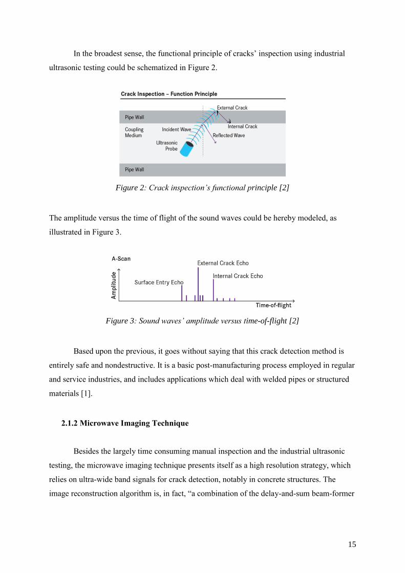
In the broadest sense, the functional principle of cracks’ inspection using industrial
ultrasonic testing could be schematized in Figure 2.
Figure 2: Crack inspection’s functional principle [2]
The amplitude versus the time of flight of the sound waves could be hereby modeled, as
illustrated in Figure 3.
Figure 3: Sound waves’ amplitude versus time-of-flight [2]
Based upon the previous, it goes without saying that this crack detection method is
entirely safe and nondestructive. It is a basic post-manufacturing process employed in regular
and service industries, and includes applications which deal with welded pipes or structured
materials [1].
2.1.2 Microwave Imaging Technique
Besides the largely time consuming manual inspection and the industrial ultrasonic
testing, the microwave imaging technique presents itself as a high resolution strategy, which
relies on ultra-wide band signals for crack detection, notably in concrete structures. The
image reconstruction algorithm is, in fact, “a combination of the delay-and-sum beam-former
16
with full-view mounted antennas” [3]. Indeed, this technique is used for both concrete or
steel based materials, however with different accounted for considerations.
Beginning with concrete, the phantom with no cracks whose dielectric properties are
previously determined (as a homogeneous material) is chosen to be the imaging domain’s
background. “As a result of this, each sensor sends UWB pulse signals to the domain and
other sensors now serve as observation points with each of them recording the received signal
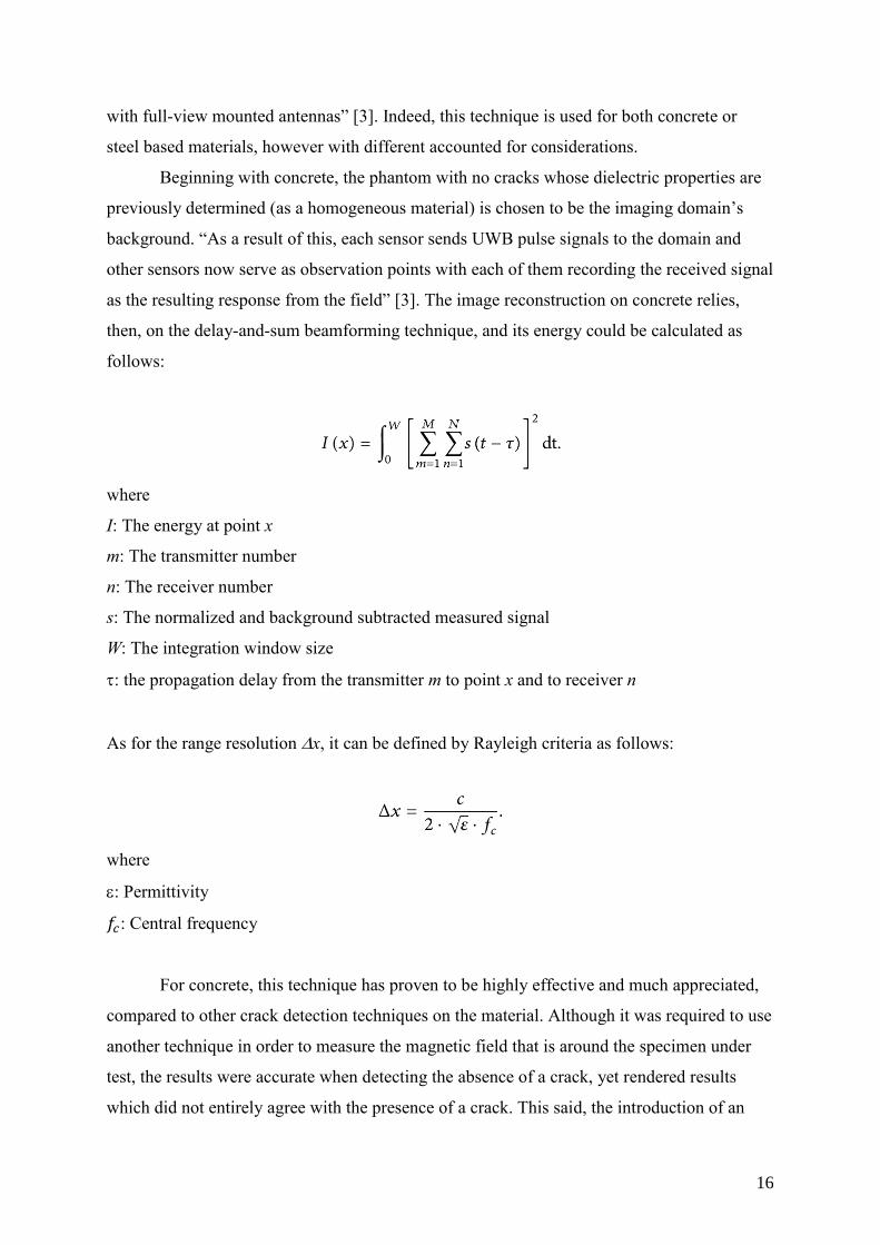
as the resulting response from the field” [3]. The image reconstruction on concrete relies,
then, on the delay-and-sum beamforming technique, and its energy could be calculated as
follows:
where
I: The energy at point x
m: The transmitter number
n: The receiver number
s: The normalized and background subtracted measured signal
W: The integration window size
: the propagation delay from the transmitter m to point x and to receiver n
As for the range resolution x, it can be defined by Rayleigh criteria as follows:
where
: Permittivity
𝑓𝑐: Central frequency
For concrete, this technique has proven to be highly effective and much appreciated,
compared to other crack detection techniques on the material. Although it was required to use
another technique in order to measure the magnetic field that is around the specimen under
test, the results were accurate when detecting the absence of a crack, yet rendered results
which did not entirely agree with the presence of a crack. This said, the introduction of an

17
additional parameter was necessary, so as to raise accuracy and enhance detection.
Nevertheless, the microwave imaging technique in concrete is cost-effective, as it bypasses
the use of ionizing radiation, and “gives a high definition image compared to ultrasonic
techniques” [3]. As a result, captures of the object under detection are much clearer,
including their peripheral areas which must also be tested.
As for steel based materials, the usage of “open-ended rectangular waveguide probes”
was suggested for the detection of cracks since the early 1990s [4]. In fact, this was mainly
introduced in order to spot “long surface cracks’ in metals. The latter refer to cracks whose
length is “greater than or equal to the broad dimension of a waveguide” [4]. For experimental
purposes, various cracks of different widths and lengths were created onto different metal
plates, and a computer-controlled stepping motor was moving the surface “over the aperture
of the open-ended waveguide while monitoring the standing-wave characteristics inside the
waveguide” [4].
Consequently, it was concluded that, when a crack’s axis is parallel to the higher
dimension of the waveguide and orthogonal to the electric field’s vector, the standing wave
undergoes a “pronounced shift” in location. Such a shift is a clear indicator of a change in the
reflection coefficient and the metal’s properties, and proves its utter dependence on the
relative emplacement of the crack as well as “the probing location on the standing wave
pattern” [4]. Figures 4 and 5 illustrate the side and front views of a crack during the process.
Figure 4: “Side view of a surface crack and an open-ended rectangular waveguide aperture”
[4]
18
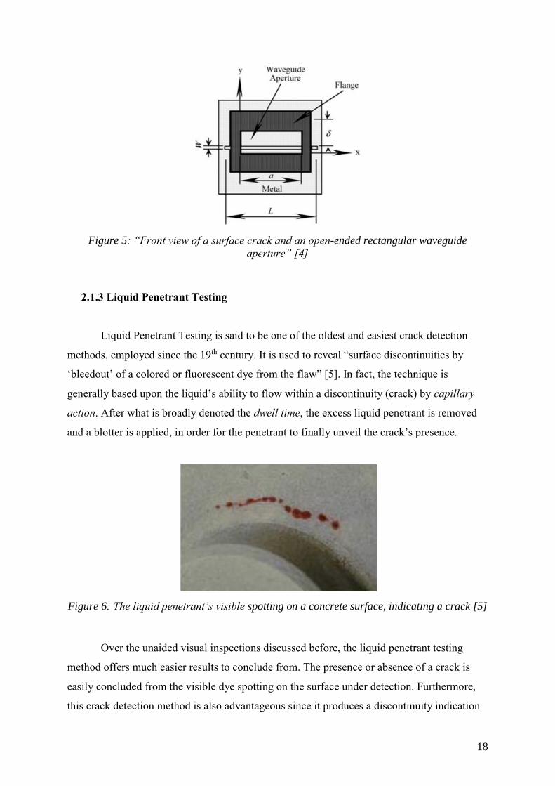
Figure 5: “Front view of a surface crack and an open-ended rectangular waveguide
aperture” [4]
2.1.3 Liquid Penetrant Testing
Liquid Penetrant Testing is said to be one of the oldest and easiest crack detection
methods, employed since the 19th century. It is used to reveal “surface discontinuities by
‘bleedout’ of a colored or fluorescent dye from the flaw” [5]. In fact, the technique is
generally based upon the liquid’s ability to flow within a discontinuity (crack) by capillary
action. After what is broadly denoted the dwell time, the excess liquid penetrant is removed
and a blotter is applied, in order for the penetrant to finally unveil the crack’s presence.
Figure 6: The liquid penetrant’s visible spotting on a concrete surface, indicating a crack [5]
Over the unaided visual inspections discussed before, the liquid penetrant testing
method offers much easier results to conclude from. The presence or absence of a crack is
easily concluded from the visible dye spotting on the surface under detection. Furthermore,
this crack detection method is also advantageous since it produces a discontinuity indication

19
that is much larger and easier to see than the crack itself. Many cracks are narrow that they
become nearly undetectable and invisible to the naked eye, but this method unveils them due
to the wider dye surface. Additionally, the high level color contrast between the surface and
the dye aids in making the distinction clearly visible [5].
Figure 7: Illustration of the larger dye covered surface compared to the flaw [5]
The exact proceeding of crack detection using the liquid penetrant testing method
may vary according to the type and size of the material being inspected, as well as the type of
flaws and discontinuities and their environments [5], however, there is a set of distinct steps
which are generally followed to perform this testing method:
Surface Preparation: “The surface must be free of oil, grease, water, or other
contaminants that may prevent the penetrant from entering flaws” [5].
Therefore, the sample under detection might require some mechanical
preparation methods such as etching, sanding, machining, or grit blasting.
Penetrant Application: After the surface has been properly cleaned and
dried, the penetrant dye “is applied by spraying, brushing, or immersing the
part in a penetrant bath” [5].
Penetrant Dwell: The penetrant is allowed enough time of incorporation into
the material, so as to seep into defects. This time is, in fact, the total time that
the liquid penetrant is put in contact with the inspected surface. “Dwell times
are usually recommended by the penetrant producers or required by the
specification being followed” [5]. Minimum dwell times are typically between
5 and 60 minutes, yet longer ones are not harmful as long as the dye is not
allowed to dry.

20
Figure 8: A penetrant being allowed dwell time [5]
Excess Penetrant Removal: After the penetrant has been allowed enough
time to dwell into the material, its excess is delicately removed from the
material’s surface, while ensuring the as little penetrant as possible is cleared.
“Depending on the penetrant system used, this step may involve cleaning with
a solvent, direct rinsing with water, or first treating the part with an emulsifier
and then rinsing water” [5].
Figure 9: Illustration of excess penetrant removal [5]
Developer Application: In order to draw the penetrant trapped in flaws back
to the surface, a very thin layer of “developer” is applied to the material,
through techniques likes “dusting” using dry powders, or spraying with wet
developers [5].
Indication Development: The developer is allowed to set for a period of time
“sufficient to permit the extraction of the trapped penetrant out of any surface
flaws” [5]. The development time is usually at least 10 minutes, however tight
cracks may require longer periods.

21
Figure 10: Illustration of the indication development phase [5]
Inspection: The inspection of crack existence if performed under adequate
lighting, in order to spot indications of flaws’ presence [5].
Clean Surface: Finally, the surface is thoroughly cleaned so as to remove any
traces of developer applied on the parts under detection [5].
2.1.4 Image Processing Technique
The Image Processing Technique to detect cracks is one of the most recent techniques
for crack detection be it inside industrial pipes, on pavements or on other surfaces that are
susceptible of becoming cracked. On the one hand, several algorithms have been proposed
and developed in order to deal with crack defects, such as an approach suggested by
AbdelQader et al. and several more. The latter proposes the usage of the “wavelet transform,
Fourier transform, Sobel filter, and Canny filter” [6]. Sinha, on the other hand, used
smoothing with morphological operations, and edge detection to perform segmentation. In a
different paper, SUSAN edge detection replaces Sobel edge detection, and instead detects
edges by “circular mask” [6]. Besides, morphological segmentation has also been used by
Tung-Ching Su et al. in order to detect fractures, open joints, debris and holes in underground
pipes [6].
The general proposed algorithm for image processing’s usage for crack detection
relies on distinct stages. The first step that must be carried out is that of image pre-
processing, which includes image gray-scaling, edge detection, noise elimination, and others.
Then, edge detection is performed using the Sobel gradient method, with an elimination of
unwanted objects [6]. After that, disjoint lines are connected and the shape of the crack, if
any, is accurately described, for the defect to be finally identified based upon its length or

22
perimeter (in the case of a hole) [6]. More details on the algorithm and the detailed steps of
crack detection using image processing will follow in this report.
2.2. Theoretical Background
There are several considerations to account for when aiming to deal with defect
detection using mechatronics. Indeed, one must be familiar with contemporary robotics, the
notion of image processing, as well as its general steps.
2.2.1 Introduction to Contemporary Robotics
Modern Robotics can be described as the “confluence science using the continuing
advancements of mechanical engineering, material science, sensor fabrication, manufacturing
techniques, and advanced algorithms” [12]. It is indeed “the science or study of the
technology primarily associated with the design, fabrication, theory, and application of
robots” [12]. With their engineered layout, robots hold the promise of performing different
tasks, among which is movement, transformation of materials, or the displacement of objects.
The most contemporary ones do more advanced tasks such as mining minerals, assembling
vehicles, are processing materials. Indeed, robotics is the realm related science and
technology, and which “stands tall by standing the accomplishments of many other fields of
study” [12].
However, robots have been inspired from nature, where all creations have been made.
That is to say that, to come up with a modern robot, it was necessary to observe the behavior
of biological creatures and mimic their behavior, in the frame of “Biometrics”. The latter is,
indeed, the study of how to imitate nature’s mechanisms and processes. Robots are, then,
programmed to perceive, decide, then act.
Perception: determines the means with which the robot will sense the environment.
These include internal sensors, such as encoders, or external ones like temperature
sensors [13]
Decision-Making: defines how the robot is going to make a decision. In fact, not all
robots are preprogrammed. Some of them adapt to their environment and learn, in the
frame of “Roboethics” [13]
Action: frames the robot’s mobility, either using wheels, legs, wings, or hybrid means
such as marsupial robots [13]

23
Figure 11 summarizes the main characteristics of contemporary robots:
Figure 11: Cycle diagram of contemporary robotics
In addition to perceiving, making decisions, and acting on the environment, a robot
must fulfill a set of functionalities, in order to be labeled contemporary. The latter line up
with its general characteristics, and are essentially their subdivisions.
Sensation: The robot must be able to sense the environment and its
surroundings. The sensors it uses are put in analogy with those used by
humans to accurately perceive the environment: “Light sensors (eyes), touch
and pressure sensors (hands), chemical sensors (nose), hearing and sonar
sensors (ears), and taste sensors (tongue)” [14]
Movement: The robot must be able to move within and around its
environment, “whether rolling on wheels, walking on legs or propelling by
thrusters” [14]. It must either move entirely, like the Sojourner robot, or have
a part of it move, such as the Canada Arm
Energy: The robot needs to be powered, either using solar or electrical
energy, or have a battery feed. Energy means depend on the robot’s specific
application
Intelligence: The robot needs to be smart, and “this is where programming
enters the picture” [14]. It is what defines what the robot needs to do, and how
it will exactly perform its tasks, according to the user’s needs
Figure 12 summarizes a modern robot’s main functionalities.
Contemporary Robotics
Perception
Decision-Making
Action
Environment

24
Figure 12: Modern robots’ main functionalities
2.2.2 Mobile Platforms
According to Ricardo Falconi, professor at Universita di Bologna, mobile robots, also
called “mobile platforms” could be defined as “automatic machines able to move into the
surrounding environment” [10]. Their characteristics include a large mobility in their
environments (land, air, water), and possess a precise level of autonomy, in addition to
limited human interaction. Such platforms are used legged or wheeled, and are used in a
number of applications:
Automatic cleaning of large areas
Client support
Support to medical services
Space exploration and remote inspection
Construction and demolishing
Material handling
Military surveillance and monitoring
Civil transportation
… [11]
Sensation Movement
Energy Intelligence
25
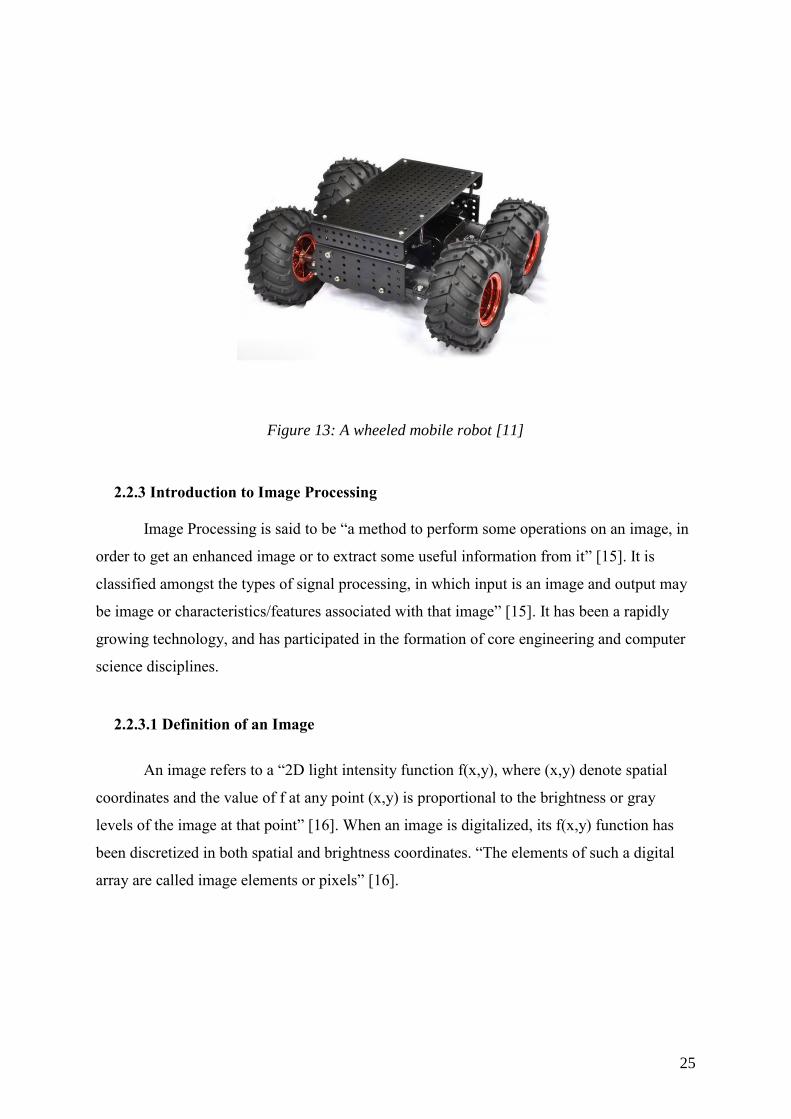
Figure 13: A wheeled mobile robot [11]
2.2.3 Introduction to Image Processing
Image Processing is said to be “a method to perform some operations on an image, in
order to get an enhanced image or to extract some useful information from it” [15]. It is
classified amongst the types of signal processing, in which input is an image and output may
be image or characteristics/features associated with that image” [15]. It has been a rapidly
growing technology, and has participated in the formation of core engineering and computer
science disciplines.
2.2.3.1 Definition of an Image
An image refers to a “2D light intensity function f(x,y), where (x,y) denote spatial
coordinates and the value of f at any point (x,y) is proportional to the brightness or gray
levels of the image at that point” [16]. When an image is digitalized, its f(x,y) function has
been discretized in both spatial and brightness coordinates. “The elements of such a digital
array are called image elements or pixels” [16].

26
Figure 14: Images of different spatial resolution [16]
2.2.3.2 Image Processing Steps
In order to perform image processing, there are a set of fundamental tools and steps
which must be followed, so as to accurately process an image and analyze its content:
1. Image Acquisition: Acquiring a digital image
2. Image Pre-processing: Improving the image in ways, in order to guarantee the
following steps’ success
3. Image Segmentation: Partitioning “an input image into its constituent parts or
objects” [16]
4. Image Representation: Converting the input data “to a suitable form for computer
processing” [16]
5. Image Description: Extracting the features that result in quantitative information, or
those that “are basic for differentiating one class of objects from another” [16]
6. Image Recognition: Assigning a label to an object “based on the information
provided by its descriptors” [16]
7. Image Interpretation: Assigning meaning to a set of recognized objects
While knowledge about a problem domain is accordingly coded “into an image
processing system in the form of a knowledge database” [16], the steps of an image’s
processing occur around such a base in order to come up with the desired result.
Figure 15 represents the fundamental steps of digital image processing summarized.
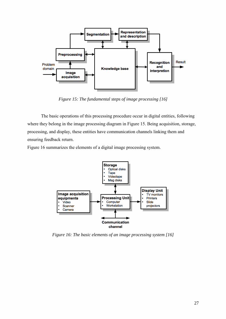
27
Figure 15: The fundamental steps of image processing [16]
The basic operations of this processing procedure occur in digital entities, following
where they belong in the image processing diagram in Figure 15. Being acquisition, storage,
processing, and display, these entities have communication channels linking them and
ensuring feedback return.
Figure 16 summarizes the elements of a digital image processing system.
Figure 16: The basic elements of an image processing system [16]

28
3. HARDWARE ARCHITECTURE AND ASSEMBLY
3.1 Hardware Components
Bearing in mind the tasks to be performed by the robot, such as motion and image
processing, we have integrated distinct electronic and mechanical components in the
platform, mounted within a functional internal architecture:
Arduino Mega 2560 R3
Raspberry Pi 3
Raspberry Pi Camera Module V2 - 8 Megapixel, 1080p
Hercules Motor Controller
USB DC-DC Converter 5V
ON-OFF Power Switch
LiPo Battery Eco-x 20C, 7.4V, 2400mAh
Magnetic Encoder Pair Kit for Micro Metal Gearmotors 12 Cycles Per Revolution
(CPR) 2.7V-18V
Sharp GP2Y0A21YK0F Analog Distance Sensor 10cm-80cm
SRF02 Ultrasonic Range Finder I2C Sensor 15cm-250cm (x2)
298:1 Micro Metal Gearmotor High-Power(HP) with Extended Motor Shaft (x4)
Smart White LEDs WS2812B
Wires
Metal frames
Chassis
Figures 17 and 18 show the most essential boards and sensors of the mobile robot.
Figure 17: Printed circuit boards (PCBs) used in the robot

29
Figure 18: Sensors used in the robot
The datasheets of the main components, as well as the dimensions of the printed circuit
boards and sensors, are found in the Appendices.
3.2 Internal Functional Architecture
In order to ensure the system’s successful operation, we made sure we followed a
precise architectural layout in interconnecting the sensors and actuators, as well as
establishing connections between the printed circuit boards, the modules, and the power
source. This said, functional architecture is defined as “an architectural model that
identifies system function and their interactions” [17]. It is the schematic with which the
operational relations between components are established, the path paver for the system
to perform its predetermined mission.
Before laying out the system’s functional architecture, it is essential to understand the
generic aspects which will be taken into account when connecting the sensors and
actuators. Figure 19 explains such aspects.
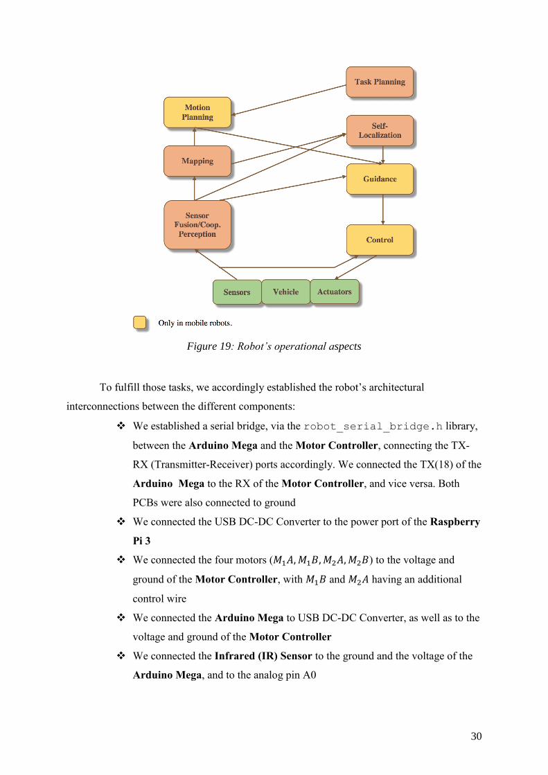
30
Figure 19: Robot’s operational aspects
To fulfill those tasks, we accordingly established the robot’s architectural
interconnections between the different components:
We established a serial bridge, via the robot_serial_bridge.h library,
between the Arduino Mega and the Motor Controller, connecting the TX-
RX (Transmitter-Receiver) ports accordingly. We connected the TX(18) of the
Arduino Mega to the RX of the Motor Controller, and vice versa. Both
PCBs were also connected to ground
We connected the USB DC-DC Converter to the power port of the Raspberry
Pi 3
We connected the four motors (𝑀1𝐴, 𝑀1𝐵, 𝑀2𝐴, 𝑀2𝐵) to the voltage and
ground of the Motor Controller, with 𝑀1𝐵 and 𝑀2𝐴 having an additional
control wire
We connected the Arduino Mega to USB DC-DC Converter, as well as to the
voltage and ground of the Motor Controller
We connected the Infrared (IR) Sensor to the ground and the voltage of the
Arduino Mega, and to the analog pin A0
31
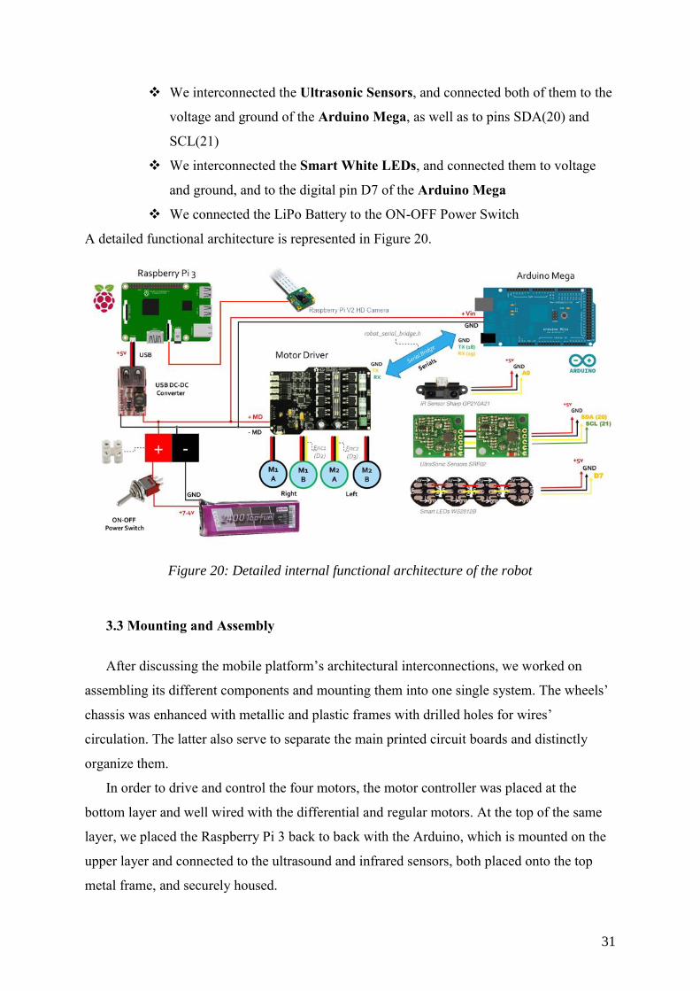
We interconnected the Ultrasonic Sensors, and connected both of them to the
voltage and ground of the Arduino Mega, as well as to pins SDA(20) and
SCL(21)
We interconnected the Smart White LEDs, and connected them to voltage
and ground, and to the digital pin D7 of the Arduino Mega
We connected the LiPo Battery to the ON-OFF Power Switch
A detailed functional architecture is represented in Figure 20.
Figure 20: Detailed internal functional architecture of the robot
3.3 Mounting and Assembly
After discussing the mobile platform’s architectural interconnections, we worked on
assembling its different components and mounting them into one single system. The wheels’
chassis was enhanced with metallic and plastic frames with drilled holes for wires’
circulation. The latter also serve to separate the main printed circuit boards and distinctly
organize them.
In order to drive and control the four motors, the motor controller was placed at the
bottom layer and well wired with the differential and regular motors. At the top of the same
layer, we placed the Raspberry Pi 3 back to back with the Arduino, which is mounted on the
upper layer and connected to the ultrasound and infrared sensors, both placed onto the top
metal frame, and securely housed.
32
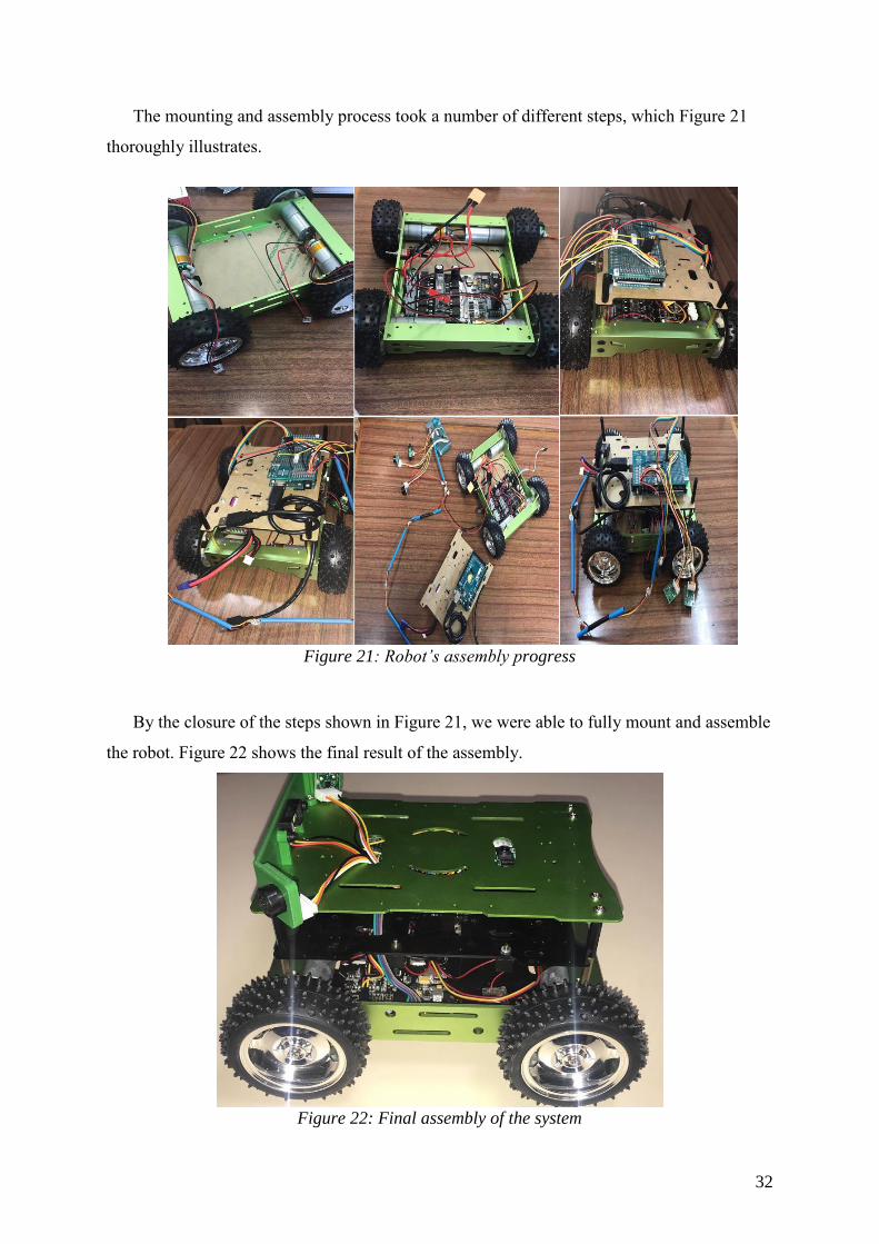
The mounting and assembly process took a number of different steps, which Figure 21
thoroughly illustrates.
Figure 21: Robot’s assembly progress
By the closure of the steps shown in Figure 21, we were able to fully mount and assemble
the robot. Figure 22 shows the final result of the assembly.
Figure 22: Final assembly of the system

33
4. COMPUTER-AIDED DESIGN OF THE ROBOT’S HOUSING
Because ensuring a compact design necessitates the housing of the sensors and
camera to be used in the design, we used 3D modelling in order to conceptualize a suitable
computer-aided design. To do so, we used FreeCAD as a 3D CAD modeler, and came up
with two alternatives.
4.1 Modeling the Sensors’ Housing - Alternative #1
We worked on the drafting of a 3D design to house the camera and sensors, and
modeled it using FreeCAD. During the process, the object’s edges were smoothened with
filets and very few acute corners were left. We ensured the model’s symmetry, and that it
entirely covers the upper part of the mobile robot. The model has two 18.5 mm in diameter
(approximately, considering a +/- 2% tolerance) holes to house the ultrasound sensors, in
addition to an intruded rectangle of approximately 30 mm in length and 10 mm in width to
house the infrared sensor. As for the LEDs, 4 small 3 mm diameter holes to house them, with
a 25 mm long very thin rectangular emplacement for the camera. Aesthetically, an extruded
three-letter label, “AUI”, was put at the top of the design, exactly centered. Thread holes
were also designed for the screws meant to fix the shell on the platform.
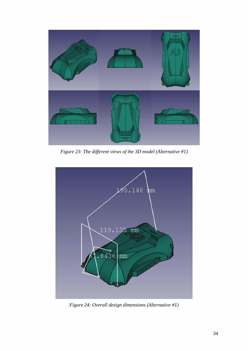
Figures 23 shows the different views of the design, while Figures 24 and 25 show the overall
dimensions of the design, as well as those of the sensors’ emplacements.
34
Figure 23: The different views of the 3D model (Alternative #1)
Figure 24: Overall design dimensions (Alternative #1)
35
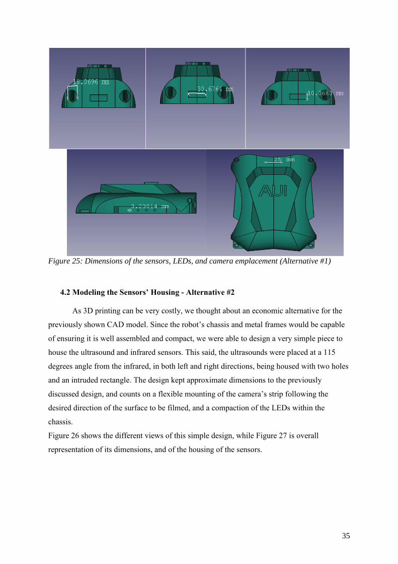
Figure 25: Dimensions of the sensors, LEDs, and camera emplacement (Alternative #1)
4.2 Modeling the Sensors’ Housing - Alternative #2
As 3D printing can be very costly, we thought about an economic alternative for the
previously shown CAD model. Since the robot’s chassis and metal frames would be capable
of ensuring it is well assembled and compact, we were able to design a very simple piece to
house the ultrasound and infrared sensors. This said, the ultrasounds were placed at a 115
degrees angle from the infrared, in both left and right directions, being housed with two holes
and an intruded rectangle. The design kept approximate dimensions to the previously
discussed design, and counts on a flexible mounting of the camera’s strip following the
desired direction of the surface to be filmed, and a compaction of the LEDs within the
chassis.
Figure 26 shows the different views of this simple design, while Figure 27 is overall
representation of its dimensions, and of the housing of the sensors.

36
Figure 26: The different views of the 3D model (Alternative #2)
Figure 27: Overall dimensions and sensors emplacement (Alternative #2)

37
5. KINEMATICS AND MOTION STUDY
5.1 Basics and Assumptions
Before engaging into the study of the mobile platform’s motion, it is substantial to
underline a set of assumptions about its kinematics. As the latter is defined as the “branch of
physics and subdivision of classical mechanics that is concerned with the geometrically
possible motion of a body” [18], it does not consider the external forces involved, nor the
causes or effects of motion. With our framed concern of ensuring our system’s motion in the
desired conditions, the forces involved in the process are of little concern to us.
For the mobile robot under study, we assume:
Differential Drive Kinematics
Forward Kinematics (The robot is assumed only to move forward and not in the
reverse direction of the pipe)
5.1.1 Differential Drive Kinematics
Seen the nature of the desired motion, the mobile platform is to adopt, for its drive
mechanism, a differential drive. By definition in the field of mobile robots, a differential
drive is a motor drive mechanism which “consists of two drive wheels mounted on a common
axis, and each wheel can independently be driven either forward or backward” [19].
While the robot’s velocity can vary, the wheels perform rolling motion as they rotate
about a point which lies along “their common left and right wheel axis” [19]. Such a point is
known as the Instantaneous Center of Curvature, or ICC for short.
Figure 28 shows the differential drive mechanism and illustrates the wheels’ shared
mounting.

38
Figure 28: Differential drive mechanism [19]
By varying the wheels’ velocity, we can systematically vary the trajectories of the
platform as well as the rate of rotation about the ICC (which must be identical for both
wheels). Following such considerations of a conditional drive, we can first schematize the
system inside an inertial frame of reference. The latter is “a reference frame in which an
object stays either at rest or at a constant velocity unless another force acts upon it” [20].
Figure 29 is a simple schematization of the robot’s emplacement inside an inertial frame of
reference.
Figure 29: Schematization of the robot’s frame within the inertial frame of reference
39
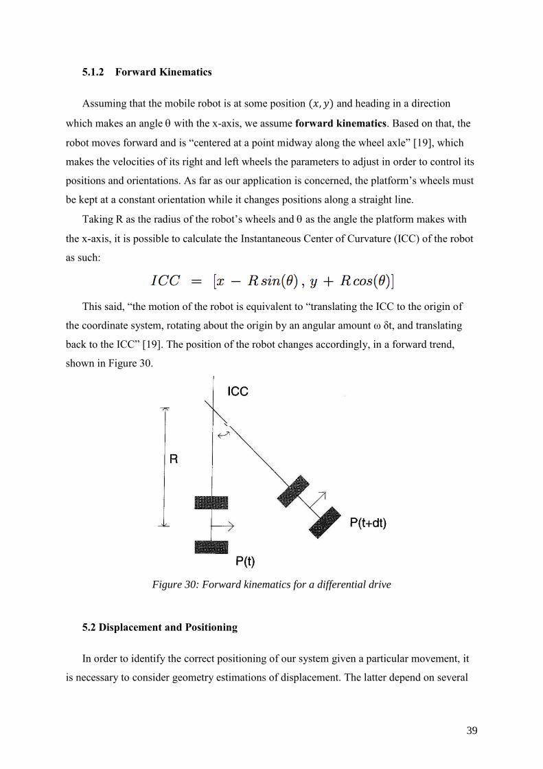
5.1.2 Forward Kinematics
Assuming that the mobile robot is at some position (𝑥, 𝑦) and heading in a direction
which makes an angle with the x-axis, we assume forward kinematics. Based on that, the
robot moves forward and is “centered at a point midway along the wheel axle” [19], which
makes the velocities of its right and left wheels the parameters to adjust in order to control its
positions and orientations. As far as our application is concerned, the platform’s wheels must
be kept at a constant orientation while it changes positions along a straight line.
Taking R as the radius of the robot’s wheels and as the angle the platform makes with
the x-axis, it is possible to calculate the Instantaneous Center of Curvature (ICC) of the robot
as such:
This said, “the motion of the robot is equivalent to “translating the ICC to the origin of
the coordinate system, rotating about the origin by an angular amount ω δt, and translating
back to the ICC” [19]. The position of the robot changes accordingly, in a forward trend,
shown in Figure 30.
Figure 30: Forward kinematics for a differential drive
5.2 Displacement and Positioning
In order to identify the correct positioning of our system given a particular movement, it
is necessary to consider geometry estimations of displacement. The latter depend on several
40
parameters, which concern the way the wheels get displaced or change orientation, either to
the left or to the right.
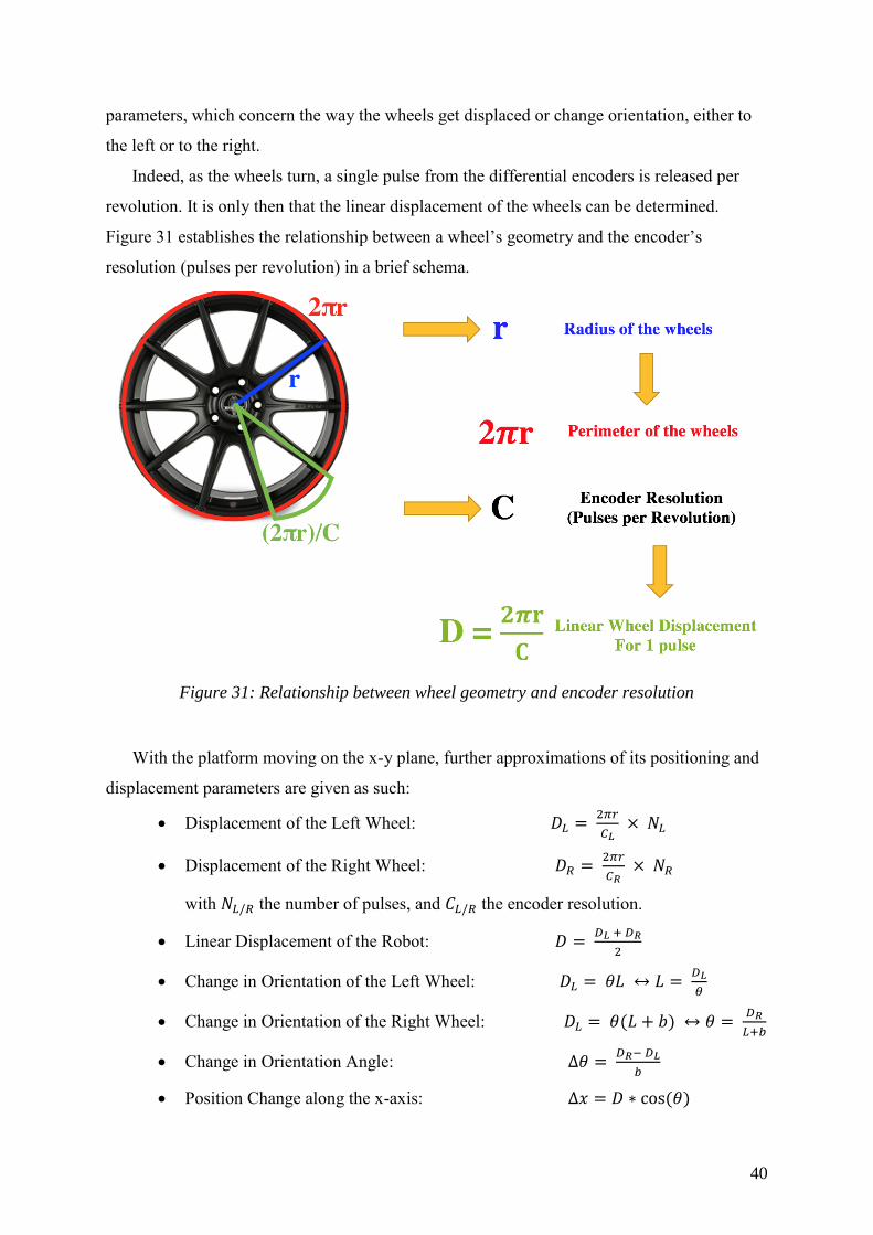
Indeed, as the wheels turn, a single pulse from the differential encoders is released per
revolution. It is only then that the linear displacement of the wheels can be determined.
Figure 31 establishes the relationship between a wheel’s geometry and the encoder’s
resolution (pulses per revolution) in a brief schema.
Figure 31: Relationship between wheel geometry and encoder resolution
With the platform moving on the x-y plane, further approximations of its positioning and
displacement parameters are given as such:
Displacement of the Left Wheel: 𝐷𝐿 = 2𝜋𝑟
𝐶𝐿 × 𝑁𝐿
Displacement of the Right Wheel: 𝐷𝑅 = 2𝜋𝑟
𝐶𝑅 × 𝑁𝑅
with 𝑁𝐿/𝑅 the number of pulses, and 𝐶𝐿/𝑅 the encoder resolution.
Linear Displacement of the Robot: 𝐷 = 𝐷𝐿 + 𝐷𝑅
2
Change in Orientation of the Left Wheel: 𝐷𝐿 = 𝜃𝐿 ↔ 𝐿 = 𝐷𝐿
𝜃
Change in Orientation of the Right Wheel: 𝐷𝐿 = 𝜃(𝐿 + 𝑏) ↔ 𝜃 = 𝐷𝑅
𝐿+𝑏
Change in Orientation Angle: ∆𝜃 = 𝐷𝑅− 𝐷𝐿
𝑏
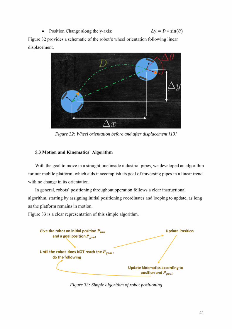
Position Change along the x-axis: ∆𝑥 = 𝐷 ∗ cos (𝜃)
41
Position Change along the y-axis: ∆𝑦 = 𝐷 ∗ sin (𝜃)
Figure 32 provides a schematic of the robot’s wheel orientation following linear
displacement.
Figure 32: Wheel orientation before and after displacement [13]
5.3 Motion and Kinematics’ Algorithm
With the goal to move in a straight line inside industrial pipes, we developed an algorithm
for our mobile platform, which aids it accomplish its goal of traversing pipes in a linear trend
with no change in its orientation.
In general, robots’ positioning throughout operation follows a clear instructional
algorithm, starting by assigning initial positioning coordinates and looping to update, as long
as the platform remains in motion.
Figure 33 is a clear representation of this simple algorithm.
Figure 33: Simple algorithm of robot positioning

42
Following the diagram in Figure 33, the robot’s position is constantly updated at
every instant t, and reveals whether it has reached its goal position yet. However, for our
platform to move straight, a few considerations must be dealt with:
The orientation must be set to zero (𝜽 = 𝟎)
Robot moves following a single axis, thus ∆𝑦 = 0
The angular velocity of the robot, as well as that of its wheels must be set to
zero (𝝎 = 𝝎𝑹 = 𝝎𝑳 = 𝟎)
Figure 34 shows the general quantities discussed for a mobile platform in motion, which must
be adjusted to our specific case.
Figure 34: Kinematics quantities scheme [13]
We have now set the goal of our robot’s motion as well as the restrictions necessary for a
desired straight motion. However, the position and velocity update component must still be
added. Referring to the initial simplified algorithm on Figure 33, it is compulsory to update
the robot’s position (and linear velocity) at every instant t, this is where the following
equations come in handy:
Position Update
𝑥𝑖+1 = 𝑥𝑖 + 𝑣𝑖+1 ∗ cos(𝜃𝑖+1)
𝑦𝑖+1 = 𝑦𝑖 + 𝑣𝑖+1 ∗ sin (𝜃𝑖+1)
Velocity Update
43
𝑣𝑖+1 = 2𝜋𝑟
𝐶∗
𝑁𝑅 + 𝑁𝐿
2∗
1
Δ𝑡
The quantities used in these equations were previously mentioned in section 5.2.
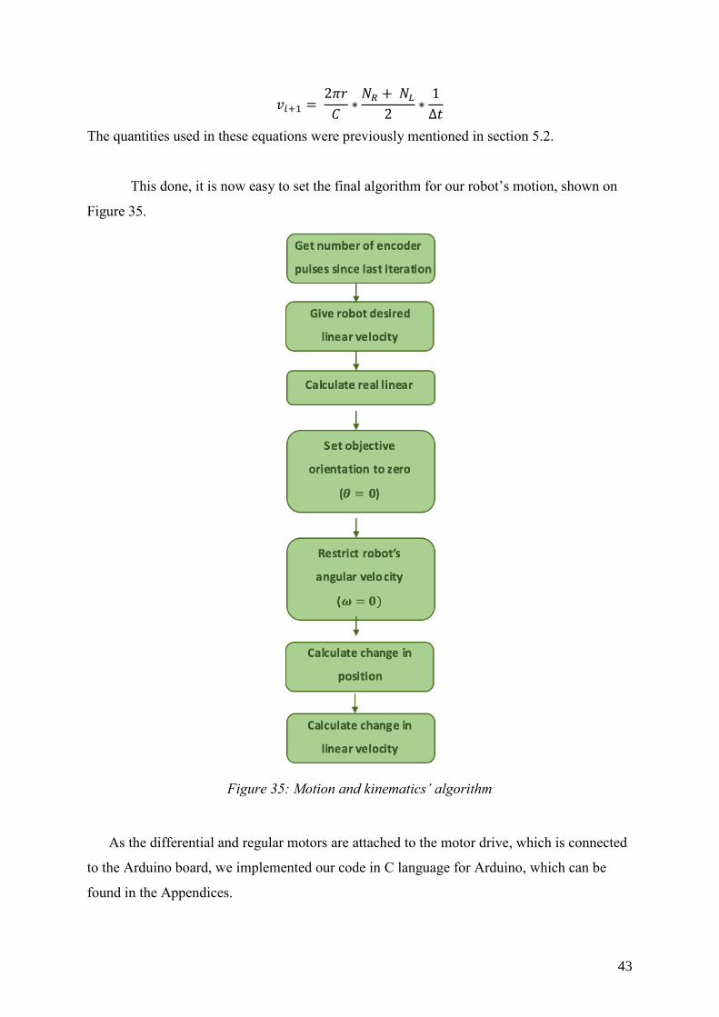
This done, it is now easy to set the final algorithm for our robot’s motion, shown on
Figure 35.
Figure 35: Motion and kinematics’ algorithm
As the differential and regular motors are attached to the motor drive, which is connected
to the Arduino board, we implemented our code in C language for Arduino, which can be
found in the Appendices.
44
6. PLATFORM CONTROL
Although the mobile robot’s velocity might be set to a desired value, it is still necessary
to add a control function to monitor the platform’s behavior. In fact, this is substantial for a
number of situational reasons. For instance, if the robot were to be stuck in an emplacement
for some reason, the wheels must compensate for each other in order for the platform to
move. Had we solely kept the algorithm shown on Figure 35, the wheels would carry on
rotating at the initial speed and would not compensate for each other nor try to advance
despite being stuck. Such boosting parameters to aid the robot overcome undesirable
situations are introduced by control, and must be called upon in most engineering
applications.
6.1 Control Theory
In applied mathematics, Control Theory is defined as “the conditions needed for a system
to maintain a controlled output in the face of input variation” [21]. As it was classically
developed for the field of robotics, this theory has been widely used in regulatory processes
for automated robots, and has its own terminology:
System: “An interconnection of elements and devices for a desired purpose”
[22]
Control System: “An interconnection of components forming a system
configuration that will provide a desired response” [22]
Process: “The device, plant, or system under control. The input and output
relationship represents the cause-and-effect relationship of the process” [22]
Therefore, control is very much involved in the autonomy of the robot. In fact, it is what
shapes its entire behavior, starting from the moment we assign its initial parameters (i.e.
velocity and position) to the time it renders a final output, be it desired or undesired.
Figure 36 suggests an overall schematic for the involvement of control laws, command, the
environment, and other parameters in shaping the robot’s behavior.

45
Figure 36: Schematic of the involvement of different components in control
6.2 Control Method – PID Controller
There are a number of methods to perform the platform control job and ensure that the
conditions needed for our robot’s optimum functioning are maintained. In essence, a robot
controller is “a combination of hardware and software to program and control a single or
multiple robots” [23]. However, there exists a wide range of platform controllers which
directly apply mathematical formulas to control desired plants, without the absolute need of
additional hardware.
Among such controllers is the famous PID Controller, which is broadly used in industry.
Indeed, the latter is “a control loop feedback mechanism”, which “continuously calculates an
error value e(t) as the difference between a desired set point and a measured process variable”
[24]. During the process, the PID controller applies corrections based upon proportional,
integral and derivative parameters, which in fact give it its name.
6.2.1 PID Controller’s Coefficients
As a matter of fact, the PID controller’s coefficients are almost proportional to a number
of behavioral reactions of the robot’s wheels. As we change those parameters, we are able to
46
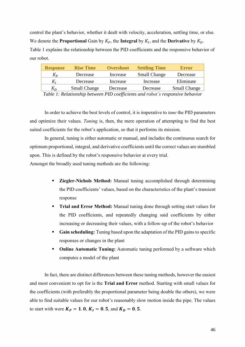
control the plant’s behavior, whether it dealt with velocity, acceleration, settling time, or else.
We denote the Proportional Gain by 𝐾𝑃, the Integral by 𝐾𝐼, and the Derivative by 𝐾𝐷.
Table 1 explains the relationship between the PID coefficients and the responsive behavior of
our robot.
Response Rise Time Overshoot Settling Time Error
𝐾𝑃 Decrease Increase Small Change Decrease
𝐾𝐼 Decrease Increase Increase Eliminate
𝐾𝐷 Small Change Decrease Decrease Small Change
Table 1: Relationship between PID coefficients and robot’s responsive behavior
In order to achieve the best levels of control, it is imperative to tune the PID parameters
and optimize their values. Tuning is, then, the mere operation of attempting to find the best
suited coefficients for the robot’s application, so that it performs its mission.
In general, tuning is either automatic or manual, and includes the continuous search for
optimum proportional, integral, and derivative coefficients until the correct values are stumbled
upon. This is defined by the robot’s responsive behavior at every trial.
Amongst the broadly used tuning methods are the following:
Ziegler-Nichols Method: Manual tuning accomplished through determining
the PID coefficients’ values, based on the characteristics of the plant’s transient
response
Trial and Error Method: Manual tuning done through setting start values for
the PID coefficients, and repeatedly changing said coefficients by either
increasing or decreasing their values, with a follow-up of the robot’s behavior
Gain scheduling: Tuning based upon the adaptation of the PID gains to specific
responses or changes in the plant
Online Automatic Tuning: Automatic tuning performed by a software which
computes a model of the plant
In fact, there are distinct differences between these tuning methods, however the easiest
and most convenient to opt for is the Trial and Error method. Starting with small values for
the coefficients (with preferably the proportional parameter being double the others), we were
able to find suitable values for our robot’s reasonably slow motion inside the pipe. The values
to start with were 𝑲𝑷 = 𝟏. 𝟎, 𝑲𝑰 = 𝟎. 𝟓, and 𝑲𝑫 = 𝟎. 𝟓.

47
After several changes made to the PID coefficients to find the best suited values, we
noticed that the wheels’ behavior altered in accordance with whether either the coefficients
increased or decreased. This said, certain conclusions were experimentally drawn as follows:
If the wheels tilt or stop abruptly, the Proportional Coefficient 𝐾𝑃 must be
decreased
If the wheels turn very slowly, the Integral Coefficient 𝐾𝐼 must be increased
If the wheels turn very fast, the Derivative Coefficient 𝐾𝐷 must be increased
The optimum values for the PID coefficients which we were able to find are the following:
𝑲𝑷 = 𝟎. 𝟖 , 𝑲𝑰 = 𝟐. 𝟓 , 𝑲𝑫 = 𝟎. 𝟎𝟐
6.2.2 PID Algorithm
After the PID coefficients have been defined and determined, an algorithm for the PID
function must be developed and added to the kinematics code. However, since the
proportional error of the controller depends on the desired and real angular and linear speeds
of the wheels, these must first be calculated.
With the desired linear speed set for our robot being 𝒗 = 𝟏 𝒎/𝒔 and its angular speed
being 𝝎 = 𝟎 𝒓𝒂𝒅/𝒔, we define the steps to be followed before calculating the PID errors as
such:
Calculate the desired angular velocities of the wheels, 𝜔𝐿𝑑 and 𝜔𝑅
𝑑
𝜔𝐿𝑑 =
𝑣𝑑−(𝑏
2∗𝜔𝑑)
𝑟 ; 𝜔𝑅
𝑑 = 𝑣𝑑+(
𝑏
2∗𝜔𝑑)
𝑟
Run the kinematics algorithm on Figure 35
Calculate the real angular velocities of the wheels, 𝜔𝐿 and 𝜔𝑅
𝜔𝐿 = 𝑣−(
𝑏
2∗𝜔)
𝑟 ; 𝜔𝑅 =
𝑣+(𝑏
2∗𝜔)
𝑟
Run the PID algorithm
Figure 37 shows the PID function’s algorithm.

48
Figure 37: PID function’s algorithm
The Arduino implementation of this algorithm is also part of the code in the Appendices.

49
7. POSITION TRACKING USING EXTERNAL SENSORS
While the robot is in operation inside a pipe, it is primordial to know whether it has exit
or if it is still within its targeted environment. Therefore, we have equipped the robot with
external sensors which would provide accurate and instantaneous feedback about the distance
covered by the platform as it is moving inside the pipe and approaching the exit. Given the
length of the pipe, the distances returned by the sensors would give an accurate idea about the
expected remaining distance for the wheeled robot to exit. This section provides algorithms
for retrieving the sensors’ readings, whose implementation is given in the Appendices.
7.1 Rotary Encoders
In order to get a timely feedback about the robot’s positioning at an instant t, our mobile
robot has been equipped with rotary encoders which return analog values corresponding to
the platform’s position and motion. Also called “shaft encoders”, rotary encoders are defined
as “electro-mechanical devices that convert the angular position or motion of the shaft or axle
to an analog or digital signal” [25].
Figure 38: Rotary encoder [25]
In fact, getting the encoders’ analog values is simply done through serial bridging. As the
rotary encoders –shown on Figure 38– are directly attached to the differential motors which
are linked to the motor drive, their analog values can easily be recorded and acquired through
Arduino’s serial monitor. The steps to follow to achieve that are:
50
Include the open-source library <robot_serial_bridge.h>
Define a serial terminal of type robot_serial_bridge
Define a structure, and declare in it variables of type long int, to carry the
encoders’ analog values
Use <serial terminal’s name>.get_encoders(<element1 of
structure>, <element2 of structure>) in order to get the analog
values of the encoders,
and <serial terminal’s name>.get_encoders_diff(<element1
of structure>, <element2 of structure>) to get the analog
values of the encoders wired to the differential motors
This way, the analog values of the rotary encoders are recorded and interpreted so as to know
the robot’s emplacement at any instant t.
7.2 Ultrasonic Sensors
7.2.1 Concept and Operation
Another approach to tracking our robot as it performs its job is to periodically check
its distance from the walls of the pipe. As the latter would become unbounded by these walls
the moment it exits, getting the values given by our two ultrasonic sensors would serve as an
indication. In fact, as the robot exits, the values sent by the sensors would abruptly change
into very high or very low values, compared to the ones shared with the serial monitor
throughout the crack detection.
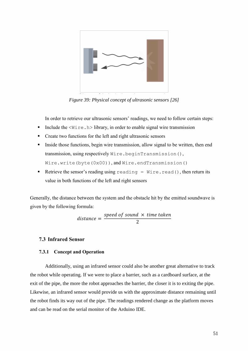
An ultrasonic sensor is defined as “a device that can measure the distance to an object
by using sound waves” [26]. It emits sound waves which hit an obstacle and come back with
an analog value corresponding to the distance traversed between the carrying device (the
robot, in our case) and the obstacle. As the signal bounces back, the time elapsed between the
emittance and reception of the wave provides us with the distance between the system and its
nearby barrier. Figure 39 is a schematic of the physical concept of an ultrasound sensor.
51
Figure 39: Physical concept of ultrasonic sensors [26]
In order to retrieve our ultrasonic sensors’ readings, we need to follow certain steps:
Include the <Wire.h> library, in order to enable signal wire transmission
Create two functions for the left and right ultrasonic sensors
Inside those functions, begin wire transmission, allow signal to be written, then end
transmission, using respectively Wire.beginTransmission(),
Wire.write(byte(0x00)), and Wire.endTransmission()
Retrieve the sensor’s reading using reading = Wire.read(), then return its
value in both functions of the left and right sensors
Generally, the distance between the system and the obstacle hit by the emitted soundwave is
given by the following formula:
𝑑𝑖𝑠𝑡𝑎𝑛𝑐𝑒 = 𝑠𝑝𝑒𝑒𝑑 𝑜𝑓 𝑠𝑜𝑢𝑛𝑑 × 𝑡𝑖𝑚𝑒 𝑡𝑎𝑘𝑒𝑛
2
7.3 Infrared Sensor
7.3.1 Concept and Operation
Additionally, using an infrared sensor could also be another great alternative to track
the robot while operating. If we were to place a barrier, such as a cardboard surface, at the
exit of the pipe, the more the robot approaches the barrier, the closer it is to exiting the pipe.
Likewise, an infrared sensor would provide us with the approximate distance remaining until
the robot finds its way out of the pipe. The readings rendered change as the platform moves
and can be read on the serial monitor of the Arduino IDE.
52
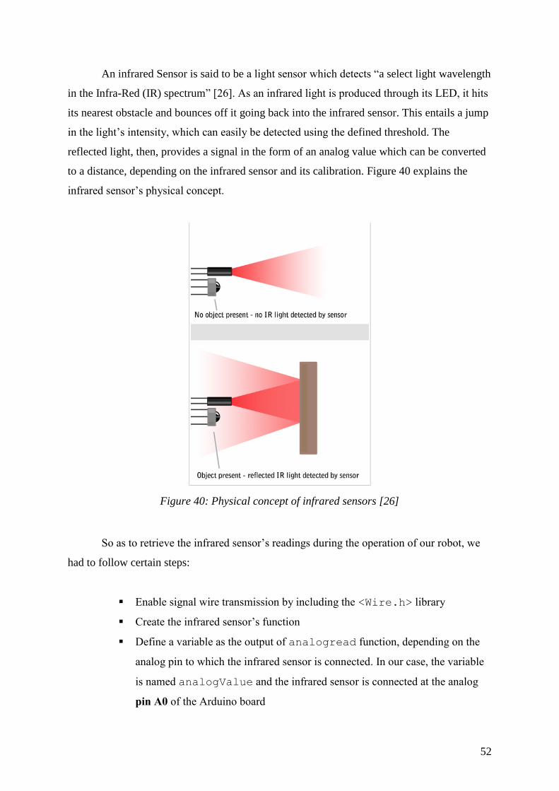
An infrared Sensor is said to be a light sensor which detects “a select light wavelength
in the Infra-Red (IR) spectrum” [26]. As an infrared light is produced through its LED, it hits
its nearest obstacle and bounces off it going back into the infrared sensor. This entails a jump
in the light’s intensity, which can easily be detected using the defined threshold. The
reflected light, then, provides a signal in the form of an analog value which can be converted
to a distance, depending on the infrared sensor and its calibration. Figure 40 explains the
infrared sensor’s physical concept.
Figure 40: Physical concept of infrared sensors [26]
So as to retrieve the infrared sensor’s readings during the operation of our robot, we
had to follow certain steps:
Enable signal wire transmission by including the <Wire.h> library
Create the infrared sensor’s function
Define a variable as the output of analogread function, depending on the
analog pin to which the infrared sensor is connected. In our case, the variable
is named analogValue and the infrared sensor is connected at the analog
pin A0 of the Arduino board

53
Do curve fitting so as to define the function which governs the signal-distance
conversion of the analog values rendered by the infrared sensor
7.3.2 Experimentation and Curve Fitting
Seen that the infrared sensor provides us with analog values as feedback for the
robot’s distance vis-à-vis its first obstacle ahead, such values must be converted into distance
values easily interpreted by the user. One of doing so was placing an obstacle in front of our
infrared sensor at different distances and recording the corresponding analog values returned
at each emplacement. An array of values, which had analog values and distances in
centimeters, has then been imported as a matrix to MATLAB, which allowed us to come up
with a curve. Performing curve fitting, the curve was fitted to an equation, which described
the relationship between the analog values and distances, and has become a conversion tool
to be used for knowing the robot’s remaining distance to exit at every instant t.
Table 2 provides the experimentally measured distances as well as their corresponding analog
values.
Distances
(cm)
Analog values
returned
15 334
17 296
20 261
23 229
25 217
27 202
30 192
33 169
35 161
40 145
43 137
45 133
50 128
55 110
60 106
65 98
70 94
75 90
Table 2: Experimentally measured distances and analog values
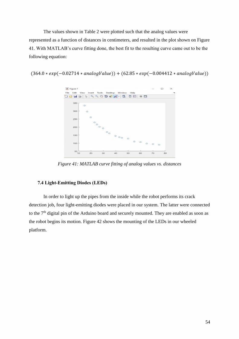
54
The values shown in Table 2 were plotted such that the analog values were
represented as a function of distances in centimeters, and resulted in the plot shown on Figure
41. With MATLAB’s curve fitting done, the best fit to the resulting curve came out to be the
following equation:
(364.0 ∗ 𝑒𝑥𝑝(−0.02714 ∗ 𝑎𝑛𝑎𝑙𝑜𝑔𝑉𝑎𝑙𝑢𝑒)) + (62.85 ∗ 𝑒𝑥𝑝(−0.004412 ∗ 𝑎𝑛𝑎𝑙𝑜𝑔𝑉𝑎𝑙𝑢𝑒))
Figure 41: MATLAB curve fitting of analog values vs. distances
7.4 Light-Emitting Diodes (LEDs)
In order to light up the pipes from the inside while the robot performs its crack
detection job, four light-emitting diodes were placed in our system. The latter were connected
to the 7th digital pin of the Arduino board and securely mounted. They are enabled as soon as
the robot begins its motion. Figure 42 shows the mounting of the LEDs in our wheeled
platform.

55
Figure 42: The system’s light-emitting diodes
7.5 Sensors’ Arduino Code – Overall Summary
After determining the sensors’ appropriate usage to knowing the robot’s emplacement
with respect to time, such information must be communicated to the Arduino board,
responsible for monitoring the sensors and actuators of our system. Having set a brief
algorithm for every sensor, these were converted into functions inside the Arduino code
given in the Appendices. Figure 43 gives the functions responsible for getting the sensors’
readings from our sensors.
Figure 43: Arduino code – Summary of sensor functions

56
8. RASPBERRY PI SET-UP AND SOFTWARE MANAGEMENT
In order to begin working on the computer vision part of our project, which is going
to take place on our tiny computer, the Raspberry Pi 3, it is first essential to install the
necessary tools to work with. Often called a “single-board computer”, the Raspberry Pi is
defined as “a credit-card sized computer that plugs into a computer monitor or TV, and uses a
standard keyboard and mouse” [27]. The latter supports several operating systems, among
which some are non-Linux-based such as NetBSD and Windows 10 IoT Code, and others
which are Linux-based such as Gentoo Linux, Ubuntu, and others.
8.1 Board Set-Up
In our project, we are using the 3rd version of the Raspberry Pi, named the Raspberry
Pi 3. Indeed, setting up the latter and working with it is quite an easy process, after making
the necessary connections:
Power: We powered the board via its power port with a laptop, using a micro
USB to USB cable
Keyboard and Mouse Connections: We connected the board to a standard
keyboard and mouse through its two USB ports
HDMI Display: In order to display the Raspberry Pi’s GUI and terminal, we
connected it to a monitor via its HDMI port, using an HDMI-DVI cable
Wi-Fi Network or Ethernet: Once the Raspberry Pi was powered, it was
connected to a nearby Wi-Fi network, and we also connected it to a local
network using its Ethernet port
Raspberry Pi Camera Connection: We connected the Raspberry Pi V2 HD
Camera to its corresponding CSI port on the board
All ports are clearly shown on the port layout sketch of the Raspberry Pi 3 on Figure 44.
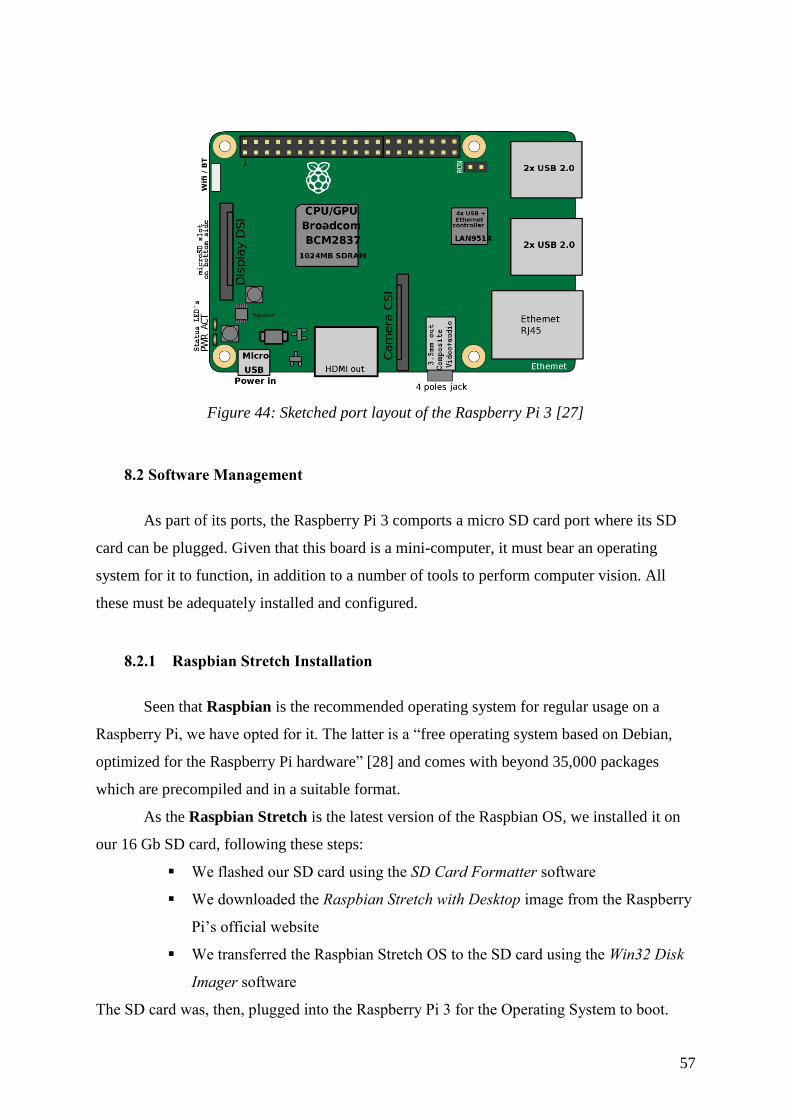
57
Figure 44: Sketched port layout of the Raspberry Pi 3 [27]
8.2 Software Management
As part of its ports, the Raspberry Pi 3 comports a micro SD card port where its SD
card can be plugged. Given that this board is a mini-computer, it must bear an operating
system for it to function, in addition to a number of tools to perform computer vision. All
these must be adequately installed and configured.
8.2.1 Raspbian Stretch Installation
Seen that Raspbian is the recommended operating system for regular usage on a
Raspberry Pi, we have opted for it. The latter is a “free operating system based on Debian,
optimized for the Raspberry Pi hardware” [28] and comes with beyond 35,000 packages
which are precompiled and in a suitable format.
As the Raspbian Stretch is the latest version of the Raspbian OS, we installed it on
our 16 Gb SD card, following these steps:
We flashed our SD card using the SD Card Formatter software
We downloaded the Raspbian Stretch with Desktop image from the Raspberry
Pi’s official website
We transferred the Raspbian Stretch OS to the SD card using the Win32 Disk
Imager software
The SD card was, then, plugged into the Raspberry Pi 3 for the Operating System to boot.

58
8.2.2 Python PiCamera Configuration
8.2.2.1 Camera Set Up
Being “a pure python interface to the Raspberry Pi” [29], the Raspberry Pi V2 HD
camera module is a library specifically written for the Raspberry Pi, using Python 2.7 or
above. With the intent to work with Python 3, the camera had to be set up, in order to be used
for capturing images of cracks.
In order to do the latter, the PiCamera module needed to be enabled and installed,
then adequately launched. We performed such operations through the following commands:
Enabling the PiCamera
Using terminal, we ran the sudo raspi-config command. Once done, a
menu appeared from which we chose to enable the PiCamera. A reboot was
required after that.
Installation the PiCamera
In order to install the python-picamera library, which is available in the
Raspbian archives, we first updated the system, then installed the Python 3
PiCamera package:
o Updating the system
sudo apt-get update
o Installing the Python 3 PiCamera package
sudo apt-get install python3-picamera
Testing the PiCamera
After the camera has been properly configured, we tested its operation by
capturing sample images. First, we accessed the Python prompt –by simply typing
“python” as a command line in terminal– (Assuming Python 3 has been installed –
See section 9.1) then imported the camera. After that, we made the camera
recognized, then captured a sample image:
o Importing the PiCamera
import picamera
o Creating an instance of the PiCamera
camera = picamera.PiCamera()
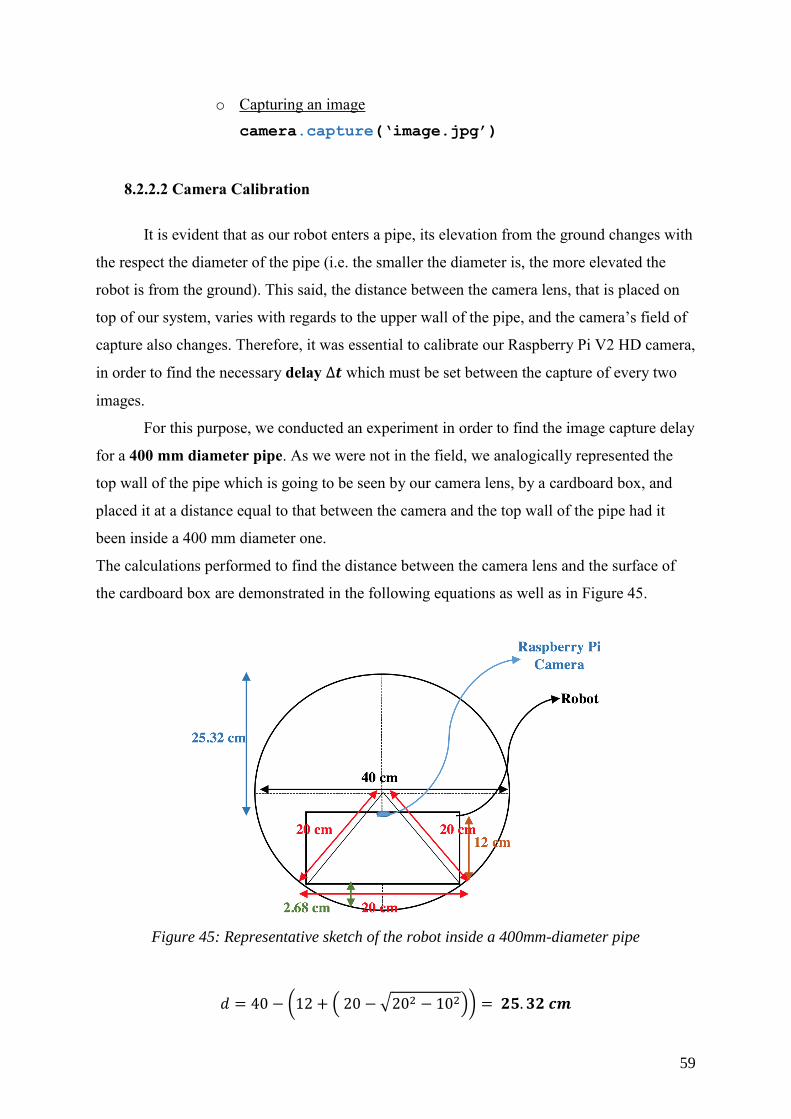
59
o Capturing an image
camera.capture(‘image.jpg’)
8.2.2.2 Camera Calibration
It is evident that as our robot enters a pipe, its elevation from the ground changes with
the respect the diameter of the pipe (i.e. the smaller the diameter is, the more elevated the
robot is from the ground). This said, the distance between the camera lens, that is placed on
top of our system, varies with regards to the upper wall of the pipe, and the camera’s field of
capture also changes. Therefore, it was essential to calibrate our Raspberry Pi V2 HD camera,
in order to find the necessary delay ∆𝒕 which must be set between the capture of every two
images.
For this purpose, we conducted an experiment in order to find the image capture delay
for a 400 mm diameter pipe. As we were not in the field, we analogically represented the
top wall of the pipe which is going to be seen by our camera lens, by a cardboard box, and
placed it at a distance equal to that between the camera and the top wall of the pipe had it
been inside a 400 mm diameter one.
The calculations performed to find the distance between the camera lens and the surface of
the cardboard box are demonstrated in the following equations as well as in Figure 45.
Figure 45: Representative sketch of the robot inside a 400mm-diameter pipe
𝑑 = 40 − (12 + ( 20 − √202 − 102)) = 𝟐𝟓. 𝟑𝟐 𝒄𝒎

60
Now that we know the distance that exists between the robot and the top wall of a 400
mm diameter pipe, we placed our system 25.32 cm away from the cardboard surface as
shown in Figure 64. We launched the image capturing simultaneously and examined the
resulting images.
Figure 46: The image calibration experiment
As a result of the experiment, the scope of the V2 HD Camera captured about a 23 cm
high image, as illustrated in Figure 46. Let h be that distance. And given that the desired
linear speed of our robot is 𝑣 = 1 𝑚/𝑠 (See section 6.2.2), the delay between every two
images must be:
∆𝑡 =ℎ
𝑣=
23 × 10−2
1= 𝟎. 𝟐𝟑 𝒔
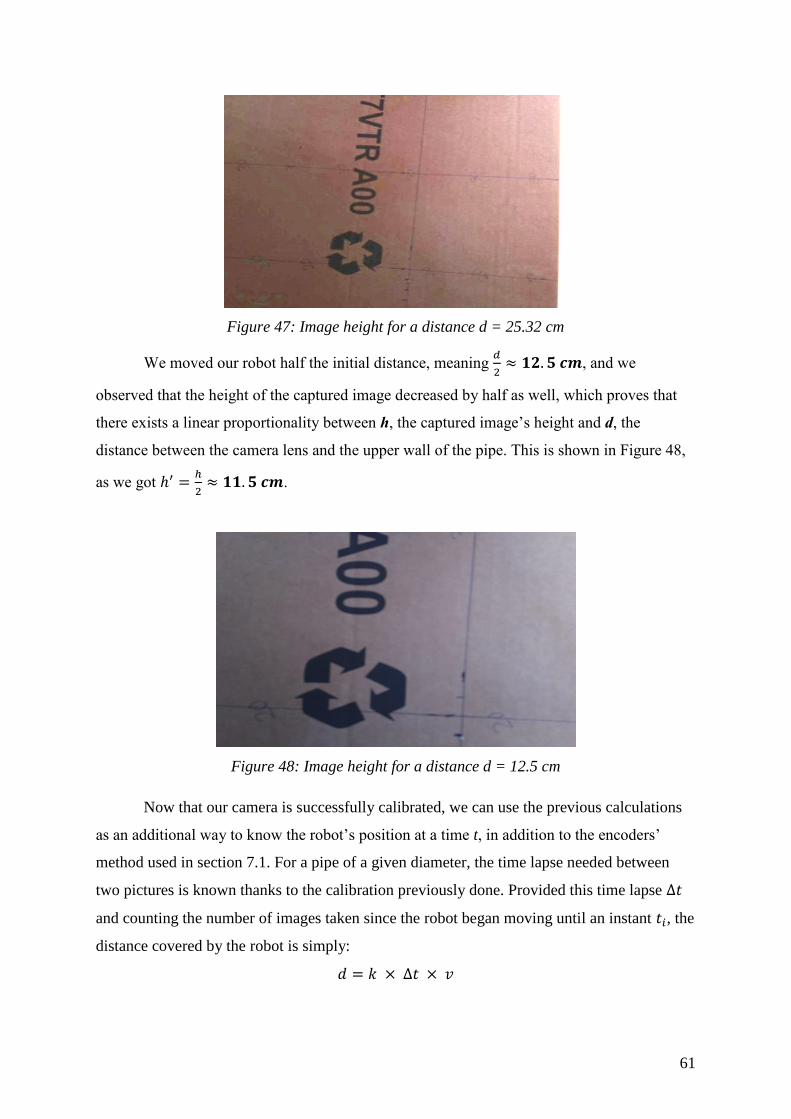
61
Figure 47: Image height for a distance d = 25.32 cm
We moved our robot half the initial distance, meaning 𝑑
2≈ 𝟏𝟐. 𝟓 𝒄𝒎, and we
observed that the height of the captured image decreased by half as well, which proves that
there exists a linear proportionality between h, the captured image’s height and d, the
distance between the camera lens and the upper wall of the pipe. This is shown in Figure 48,
as we got ℎ′ =ℎ
2≈ 𝟏𝟏. 𝟓 𝒄𝒎.
Figure 48: Image height for a distance d = 12.5 cm
Now that our camera is successfully calibrated, we can use the previous calculations
as an additional way to know the robot’s position at a time t, in addition to the encoders’
method used in section 7.1. For a pipe of a given diameter, the time lapse needed between
two pictures is known thanks to the calibration previously done. Provided this time lapse ∆𝑡
and counting the number of images taken since the robot began moving until an instant 𝑡𝑖, the
distance covered by the robot is simply:
𝑑 = 𝑘 × ∆𝑡 × 𝑣
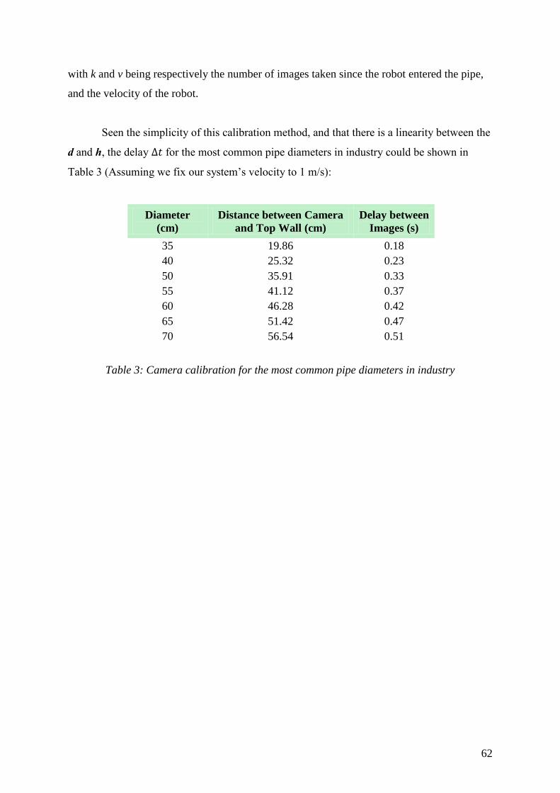
62
with k and v being respectively the number of images taken since the robot entered the pipe,
and the velocity of the robot.
Seen the simplicity of this calibration method, and that there is a linearity between the
d and h, the delay ∆𝑡 for the most common pipe diameters in industry could be shown in
Table 3 (Assuming we fix our system’s velocity to 1 m/s):
Diameter
(cm)
Distance between Camera
and Top Wall (cm)
Delay between
Images (s)
35 19.86 0.18
40 25.32 0.23
50 35.91 0.33
55 41.12 0.37
60 46.28 0.42
65 51.42 0.47
70 56.54 0.51
Table 3: Camera calibration for the most common pipe diameters in industry
63
9. REAL-TIME COMPUTER VISION AND IMAGE PROCESSING
Having installed the Raspbian Stretch, the Raspberry’s operating system, in addition
to configuring the PiCamera and calibrating it, it is now possible to use it in order to capture
images of cracks, then employ the operating system’s user interface in order to treat images
and process them.
One of the most prominent and available tools to perform computer vision is
OpenCV. The latter is “an open source computer vision and machine learning software
library” [30] which contains a number of programming functions, capable of performing real-
time computer vision. In this project, the main aim is to unveil the existence of cracks onto
pipes’ surfaces as the images get captured. Therefore, the employment of OpenCV, as a
potential and accurate image processer, is fundamental.
9.1 Installing OpenCV and Python 3 on Raspbian Stretch
With the intent to process and analyze the captured images using the PiCamera, the
installation of the necessary tools to do so is required. First of all, we needed to install
OpenCV as our real-time computer vision library, then installed Python 3, since most of
OpenCV’s available functions are easier to work with in Python. The image processing script
is going to be programmed using Python 3, henceforth another reason for choosing the latter.
The most important steps of the installation process are listed as follows:
Step 1: Expand the filesystem
Since we are using a brand new install of the Raspbian Stretch and have not updated it
from Raspbian Jessie, we were required to do an expansion of our filesystem, in order to
make the operating system include the entire available space on the micro SD card.
Step 2: Install dependencies
The installation of OpenCV is dependent on numerous files and package, which need
to be installed. We installed the latter, ranging from developer tools to image and videos I/Os,
in addition to the Python 3 header files.
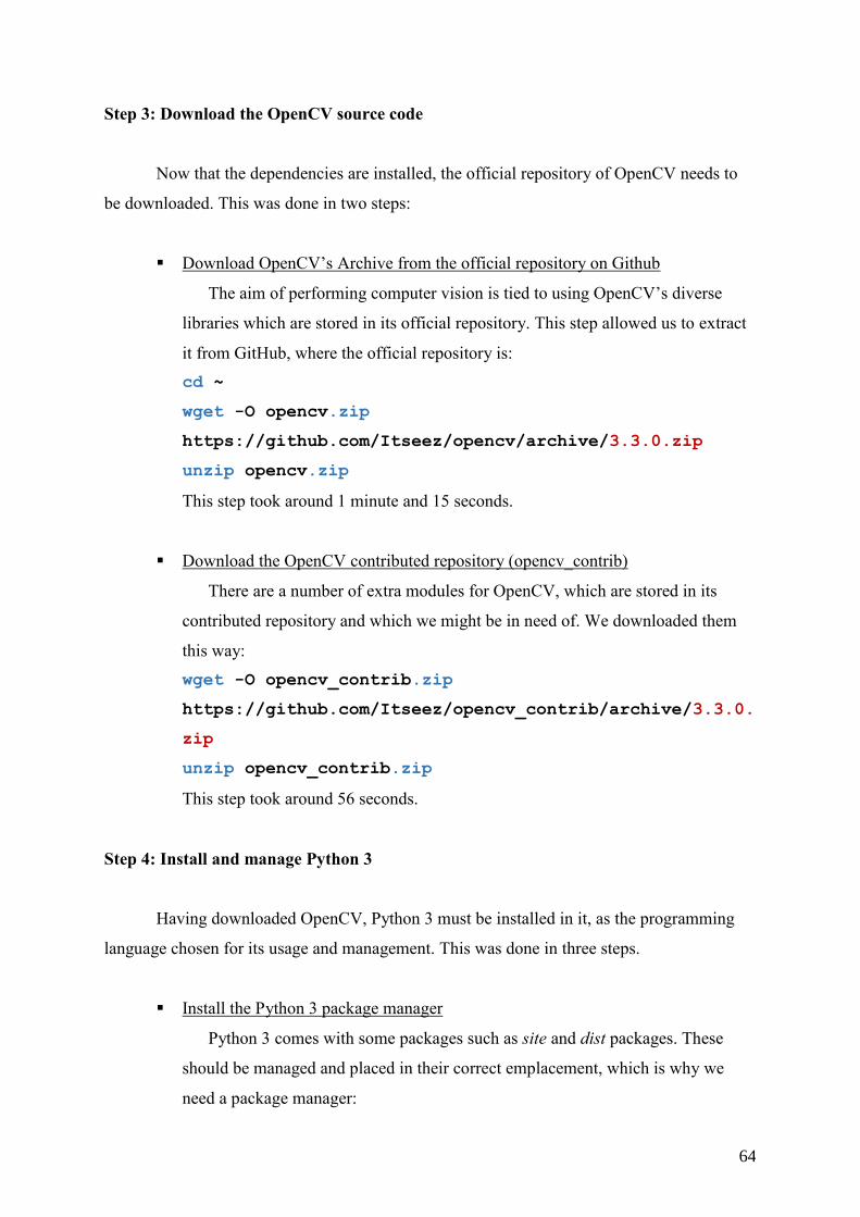
64
Step 3: Download the OpenCV source code
Now that the dependencies are installed, the official repository of OpenCV needs to
be downloaded. This was done in two steps:
Download OpenCV’s Archive from the official repository on Github
The aim of performing computer vision is tied to using OpenCV’s diverse
libraries which are stored in its official repository. This step allowed us to extract
it from GitHub, where the official repository is:
cd ~
wget -O opencv.zip
https://github.com/Itseez/opencv/archive/3.3.0.zip
unzip opencv.zip
This step took around 1 minute and 15 seconds.
Download the OpenCV contributed repository (opencv_contrib)
There are a number of extra modules for OpenCV, which are stored in its
contributed repository and which we might be in need of. We downloaded them
this way:
wget -O opencv_contrib.zip
https://github.com/Itseez/opencv_contrib/archive/3.3.0.
zip
unzip opencv_contrib.zip
This step took around 56 seconds.
Step 4: Install and manage Python 3
Having downloaded OpenCV, Python 3 must be installed in it, as the programming
language chosen for its usage and management. This was done in three steps.
Install the Python 3 package manager
Python 3 comes with some packages such as site and dist packages. These
should be managed and placed in their correct emplacement, which is why we
need a package manager:
65
wget https://bootstrap.pypa.io/get-pip.py
sudo python3 get-pip.py
This step took around 45 seconds.
Create our own Python virtual environment
It is crucial to understand that “a virtual environment is a special tool used to
keep the dependencies required by different projects in separate places by creating
isolated, independent Python environments for each of them” [31]. This is why it
was essential to install it, in order to keep our site-packages (the packages inside
the Python directory) safe.
sudo pip install virtualenv virtualenvwrapper
sudo rm -rf ~/.cache/pip
This took about 47 seconds.
After installing virtualenv, we created our own Python virtual environment,
which will be used for computer vision development.
mkvirtualenv cv -p python3
This took around 30 seconds.
Install NumPy on the Raspberry Pi
In order to perform numerical analysis (when needed), we installed a Python
dependency called NumPy. The latter works in the created virtual environment
and must be installed using pip, Python’s main package manager.
pip install numpy
Step 5: Compile and install OpenCV
Build using CMake
After making sure that we are working within the cv environment, using workon
cv, we accessed the OpenCV directory, then used the CMake package and software
builder to setup up and build example packages of OpenCV and Python.
cd ~/opencv-3.3.0/
mkdir build
cd build
cmake -D CMAKE_BUILD_TYPE=RELEASE \

66
-D CMAKE_INSTALL_PREFIX=/usr/local \
-D INSTALL_PYTHON_EXAMPLES=ON \
-D OPENCV_EXTRA_MODULES_PATH=~/opencv_contrib-
3.3.0/modules \
-D BUILD_EXAMPLES=ON ..
This took about 3 minutes and 21 seconds.
Compile OpenCV
OpenCV is now ready to compile. We compiled it and waited for around 3
hours and 40 minutes until the process finished compiling.
make -j4
Step 6: Finish installing OpenCV on the Raspberry Pi
Having downloaded, installed, and compiled OpenCV, the final step is to link the
“OpenCV bindings” to the virtual environment that we created. Those bindings are simply
linkages which make OpenCV’s algorithms, that are originally written in C++, enabled and
bridged to other language. Since our programming language is Python, we seek to bridge
OpenCV’s algorithms to Python.
Step 7: Test OpenCV’s installation
A simple test to make sure that OpenCV has been successfully installed on our
Raspberry Pi 3 is to execute the source and workon commands, then attempt to import the
bindings of both Python and OpenCV. We did that as follows:
source ~/.profile
workon cv
python
>>> import cv2
>>> cv2.__version__
'3.3.0'
>>>

67
9.2 Image Processing for Crack Detection
Now that we have our image processing tool installed and “binded” with Python 3,
our main programming language, the aim of detecting cracks inside pipelines can be
accomplished with the help of the captured images on which an adequate program will run.
The process of image processing is based upon the treatment of digitalized images, in order
to analyze their content or manipulate them.
9.2.1 Image Capturing
Using our Raspberry Pi V2 HD camera, whose resolution reaches its maximum at
3280x2464 pixels and a cadence of 30 frames per second (See datasheet in Appendices), it is
possible to capture good resolution images, exhibiting the pixels of an image, throughout
lighting variations from strong to dim. Of course, the qualities of the captures differ,
according to the light’s intensity.
As we would like our V2 HD camera to capture images with a 0.23 seconds delay,
following the calibration done for a 400 mm diameter pipe, we accounted for that in the
image capturing algorithm developed. The latter is simple and directs the storing of the
images to the images folder placed in the pi file inside home.
The path of the captured images is then as follows:
/home/pi/images/
The algorithm developed could be summarized in Figure 49.

68
Figure 49: Image capturing algorithm
The purpose of setting a counter which gets incremented every ∆𝑡 = 𝑑𝑒𝑙𝑎𝑦, is to
avoid the overwriting of newly captured images on those already existent in the images
folder. The images, thus, get all stored in the folder, having a name with a number increment
of 1, hence a different name for every image.
9.2.2 Image Processing Using OpenCV
With our Raspberry Pi V2 HD camera capturing images at a timely basis and storing
them in our desired location, the next step is to perform image processing, in order to find
whether or not cracks exist on the inside walls of industrial pipes.
69
9.2.2.1 Process Flowchart of Image Processing
According to the literature, there are several algorithms which could be followed in
order to treat an image and process it. However, following our research, the raw data, that is
the RGB (colored) imaged acquired –in our case, captured–, must be digitalized and then
preprocessed. In order to conduct the latter, the image must be stripped off its colors and
converted into shades of gray for the image processing algorithm to be functional. Indeed,
gray scaling an image is defined as “the process of converting a continuous-tone image to an
image that a computer can manipulate” [33].
Once the image is gray-scaled, it is ready for processing. Only then can it be subject
to feature detection, which is a process for quantifying the abstractions of an image and
deciding about its features. There are several features which could be found in an image,
ranging from edges, to points and corners, to blobs and ridges, and many more.
Since the core interest of this study is to unveil the existence or non-existence of cracks onto
a determined area (pipe surface), the decision of employing a certain feature detection
method must be made carefully.
Indeed, such a decision has been made with the help with a few considerations, which
could be summarized as follows:
o Why not Point Detection?
Most concrete pipes have sandy textures, and such small dots could be mistakenly
identified as points. Other points, which are not cracks, such as drops of paint or
else, could also be taken for cracks
o Why not Ridge Detection?
Cracks are not ridges. They are not curved and are necessarily sharp
o Why not Blob Detection?
Blob detection deals with areas which are characterized differently in an image.
For instance, “areas in an image which are too smooth” to be detected by a point
detector [34]. In our case, cracks are not identified over areas, yet over lines and
edges
o And, why Edge Detection?
Cracks are generally identified as edges. They are crossing lines which constitute
an elongated defect in a material
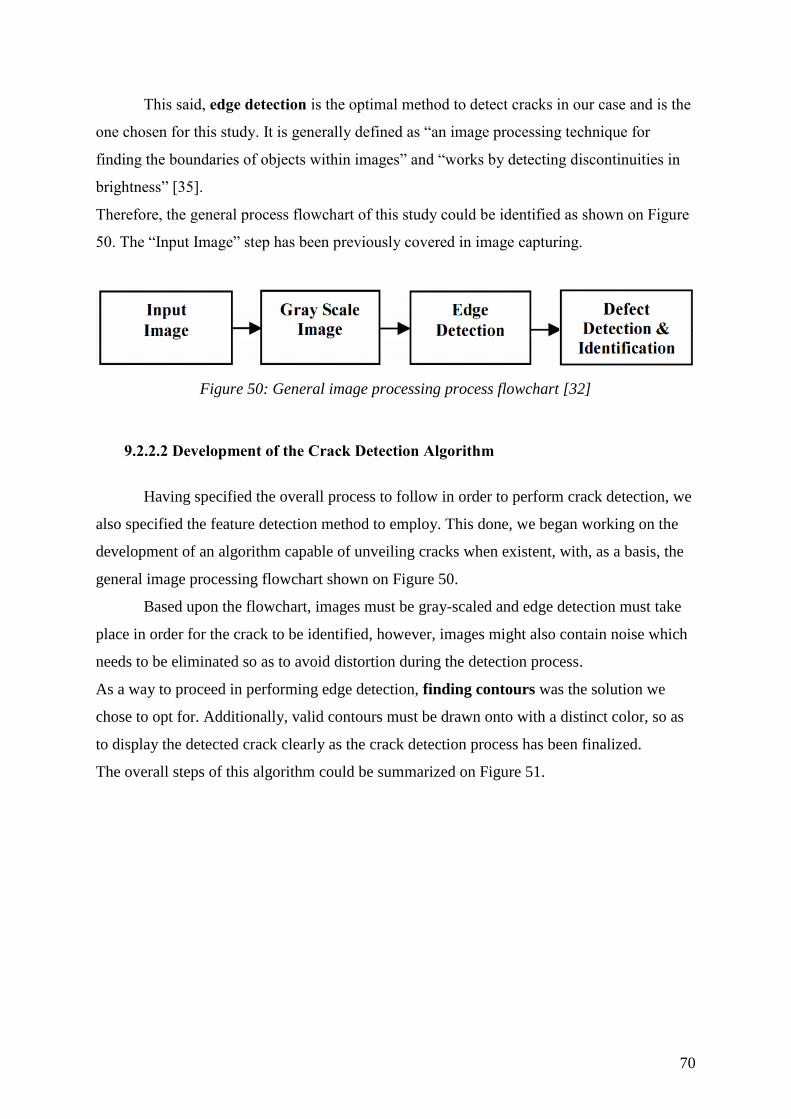
70
This said, edge detection is the optimal method to detect cracks in our case and is the
one chosen for this study. It is generally defined as “an image processing technique for
finding the boundaries of objects within images” and “works by detecting discontinuities in
brightness” [35].
Therefore, the general process flowchart of this study could be identified as shown on Figure
50. The “Input Image” step has been previously covered in image capturing.
Figure 50: General image processing process flowchart [32]
9.2.2.2 Development of the Crack Detection Algorithm
Having specified the overall process to follow in order to perform crack detection, we
also specified the feature detection method to employ. This done, we began working on the
development of an algorithm capable of unveiling cracks when existent, with, as a basis, the
general image processing flowchart shown on Figure 50.
Based upon the flowchart, images must be gray-scaled and edge detection must take
place in order for the crack to be identified, however, images might also contain noise which
needs to be eliminated so as to avoid distortion during the detection process.
As a way to proceed in performing edge detection, finding contours was the solution we
chose to opt for. Additionally, valid contours must be drawn onto with a distinct color, so as
to display the detected crack clearly as the crack detection process has been finalized.
The overall steps of this algorithm could be summarized on Figure 51.
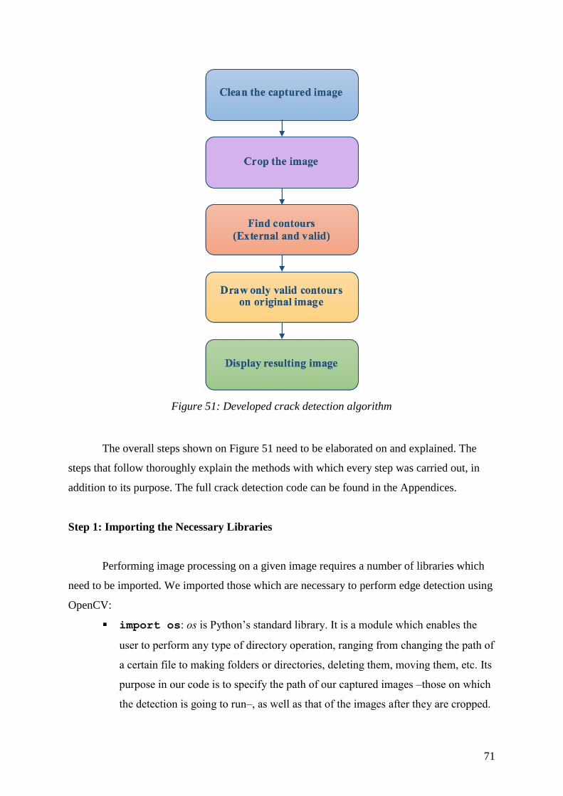
71
Figure 51: Developed crack detection algorithm
The overall steps shown on Figure 51 need to be elaborated on and explained. The
steps that follow thoroughly explain the methods with which every step was carried out, in
addition to its purpose. The full crack detection code can be found in the Appendices.
Step 1: Importing the Necessary Libraries
Performing image processing on a given image requires a number of libraries which
need to be imported. We imported those which are necessary to perform edge detection using
OpenCV:
import os: os is Python’s standard library. It is a module which enables the
user to perform any type of directory operation, ranging from changing the path of
a certain file to making folders or directories, deleting them, moving them, etc. Its
purpose in our code is to specify the path of our captured images –those on which
the detection is going to run–, as well as that of the images after they are cropped.

72
As the emplacement of our captured images (as seen in section 9.2.1) is
home/pi/images/, that of our cropped images was specified to be
home/pi/cropped/. We specified the latter as such for the detection to run
solely on the images which have been cropped (See Step 2 for more information
about the reason why images needed to be cropped).
import cv2: cv2 is OpenCV’s library and module responsible for extracting all
the operators and multi-stage algorithms which could be used to perform detection
import numpy: numpy is a library used for computational and numerical
analysis. Since our program involved a few computations, it was necessary to
import it
Step 2: Cleaning and Gray Scaling the Image
Image Denoising is the process with which distorting and unwanted elements are
removed from images. Indeed, there are a lot of image denoising algorithms in mathematics,
and several are those which come with OpenCV. In the latter, the idea is simple: We need to
“average out the noise” in an image [36]. With the help of a few functions, which we used in
our crack detection code, we were able to reduce the overall noise in pictures and smoothen
them out.
fastNlMeansDenoisingColored(): This function reduces noise in colored
images, and takes in six arguments. The first two arguments are the input array,
which is, in this case, the image itself, and the output array which we do not have in
our case (It could be the same noise reduction in another image). As for the remaining
arguments, they are the strength of the filter h, the corresponding color component
of h, the window size that is used to compute the average pixel value for each
chunk of the image size, repeated twice.
To find the correct window size, it is advised to try the multiples of 3, and examine
results one by one. While doing so, we were also changing the value of strength of the
filter choosing random values, ranging from 1 to 9. The optimal combination came
out to be:
𝑾𝒊𝒏𝒅𝒐𝒘 𝒔𝒊𝒛𝒆 = 𝟐𝟏
𝑺𝒕𝒓𝒆𝒏𝒈𝒕𝒉 𝒐𝒇 𝒕𝒉𝒆 𝒇𝒊𝒍𝒕𝒆𝒓 = 𝟕
73
Gaussian Blurring: OpenCV is provided with the Gaussian kernel, which comes
with several functions, among which is the GaussianBlur(). The latter only
supports odd numbers, and takes in the standard deviation of the blur to be applied on
the image in x and y respectively. In our case, we do not seek to blur the image much,
as this is done just in case the previous image denoising had not worked perfectly.
Thus, we only chose to have a 1 pixel blur on the x axis as well as on the y axis. As
we do not need pixel extrapolation, we set the last argument of the
GaussianBlur() to be 0.
Gray Scaling: We converted images from color to gray through the simple use of the
OpenCV function COLOR_BGR2GRAY().
Converting to Black and White: Canny() is the function which takes smoothened
images and converts them to black and white using two threshold values, a minimum
and maximum one. In order to do so, we first had to determine the median of the
image, which is the pixel difference between its highest and lowest half. Once done,
we defined a value, sigma, which is the percent of the median which is must be used
to find the correct threshold values. Sigma is generally advised to be 0.25 in Canny.
Thus, the threshold values, which must range between 0 and 255 (the range of
numerical values attributed to the scale of lighter to darker colors), were defined as
follows:
𝒕𝒉𝒓𝒆𝒔𝒉𝒐𝒍𝒅𝒎𝒊𝒏 = 𝒊𝒏𝒕(𝒎𝒂𝒙(𝟎, 𝒔𝒊𝒈𝒎𝒂 ∗ 𝒎))
𝒕𝒉𝒓𝒆𝒔𝒉𝒐𝒍𝒅𝒎𝒂𝒙 = 𝒊𝒏𝒕(𝒎𝒂𝒙(𝟐𝟓𝟓, 𝒔𝒊𝒈𝒎𝒂 ∗ 𝒎))
Step 3: Cropping Images
Following several trials to adjust the compatibility of the images captured by our
Raspberry Pi V2 HD camera with our code (See Image Compatibility Challenges for more
information), the optimal solution to make the captured images compatible with the program
so that the detection to run successfully, was cropping them.
Indeed, it was noticeable that the images taken by the V2 HD camera generally had
distorted side areas which contained useless information about the crack. The scope of the Pi
camera was large enough not to make it possible for the images to be processed. In fact, this
is due to lighting, as the contrast between the background and the crack becomes lower as we
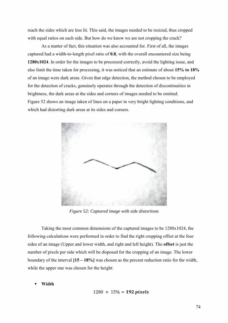
74
reach the sides which are less lit. This said, the images needed to be resized, thus cropped
with equal ratios on each side. But how do we know we are not cropping the crack?
As a matter of fact, this situation was also accounted for. First of all, the images
captured had a width-to-length pixel ratio of 0.8, with the overall encountered size being
1280x1024. In order for the images to be processed correctly, avoid the lighting issue, and
also limit the time taken for processing, it was noticed that an estimate of about 15% to 18%
of an image were dark areas. Given that edge detection, the method chosen to be employed
for the detection of cracks, genuinely operates through the detection of discontinuities in
brightness, the dark areas at the sides and corners of images needed to be omitted.
Figure 52 shows an image taken of lines on a paper in very bright lighting conditions, and
which had distorting dark areas at its sides and corners.
Figure 52: Captured image with side distortions
Taking the most common dimensions of the captured images to be 1280x1024, the
following calculations were performed in order to find the right cropping offset at the four
sides of an image (Upper and lower width, and right and left height). The offset is just the
number of pixels per side which will be disposed for the cropping of an image. The lower
boundary of the interval [15 – 18%] was chosen as the percent reduction ratio for the width,
while the upper one was chosen for the height:
Width
1280 × 15% = 𝟏𝟗𝟐 𝒑𝒊𝒙𝒆𝒍𝒔
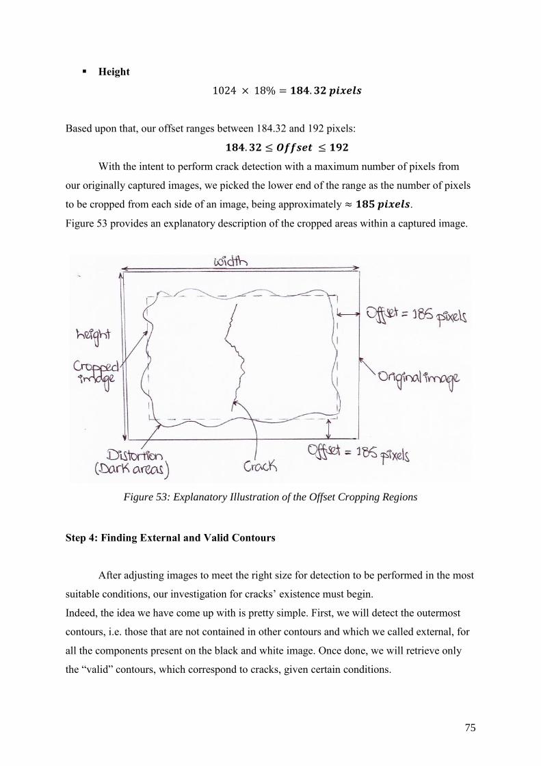
75
Height
1024 × 18% = 𝟏𝟖𝟒. 𝟑𝟐 𝒑𝒊𝒙𝒆𝒍𝒔
Based upon that, our offset ranges between 184.32 and 192 pixels:
𝟏𝟖𝟒. 𝟑𝟐 ≤ 𝑶𝒇𝒇𝒔𝒆𝒕 ≤ 𝟏𝟗𝟐
With the intent to perform crack detection with a maximum number of pixels from
our originally captured images, we picked the lower end of the range as the number of pixels
to be cropped from each side of an image, being approximately ≈ 𝟏𝟖𝟓 𝒑𝒊𝒙𝒆𝒍𝒔.
Figure 53 provides an explanatory description of the cropped areas within a captured image.
Figure 53: Explanatory Illustration of the Offset Cropping Regions
Step 4: Finding External and Valid Contours
After adjusting images to meet the right size for detection to be performed in the most
suitable conditions, our investigation for cracks’ existence must begin.
Indeed, the idea we have come up with is pretty simple. First, we will detect the outermost
contours, i.e. those that are not contained in other contours and which we called external, for
all the components present on the black and white image. Once done, we will retrieve only
the “valid” contours, which correspond to cracks, given certain conditions.

76
Detecting External Contours: It is easy to find the outermost contours in an image.
This is simply done using OpenCV’s function findContours(), which takes the
output of the Canny function, as well as two hierarchy arguments predefined by
OpenCV.
Detecting Valid Contours: Now that the external contours of an image are found, we
need to decide which of those correspond to a crack. Inside a loop, we defined a
distance d, which is the distance between two individual contours which may be part
of the crack as they may not:
o If the distance between those is less than 50% of the maximum
distance between the width and the height, then those contours are
appended and joined together
o If not, they are not likely to be part of a crack since they are too far
from each other
This is done for all neighboring contours, until those which constitute a crack are
appended to each other and the crack is correspondingly traced. However, a contour
might have neighboring contours which append to it and still not be part of the crack,
or it could be very small that it is utterly insignificant. This is why we set more
conditions on detecting valid contours:
o If a point c has neighbors which are, in total, less than 20% of the
number of points detected as part of a crack, it must not be considered
part of it itself
o If the dimensions of a point satisfy 𝒘𝒊𝒅𝒕𝒉 + 𝒉𝒆𝒊𝒈𝒉𝒕 < 𝟓 𝒑𝒊𝒙𝒆𝒍𝒔,
the point is too small and must be disregarded
Step 5: Drawing Valid Contours on the Original Image
Following the previously mentioned conditions, we now are able to spot the contours
which constitute a crack and join them in order to form what we called “valid contours”.
With the aim to trace the detected crack as an output for the detection process, we employed
one of OpenCV’s offered functions, drawContours(). The latter takes in, as arguments,
the image on which the contours will be drawn, the contours, the color with which they be
drawn, and the thickness of the line.
77
As the color we chose to draw the contours is red and that the value provided for a contour
drawer are respectively (B, G, R), we set R (red) to the maximum (255), and set the other
two values for green and blue to 0: (0, 0, 255). The thickness chosen for the line was 3, for
clarity reasons.
Step 6: Displaying the Resulting Image
To finalize the crack detection process, we need to display the result of the detection,
whether a crack was found or not. This was done through, first, resizing the display window
so that it is not too big using the resizeWindow() function, and finally using imshow()
to show the final output. At the end, the user presses a key and all windows are closed.
The full program can be found in the Appendices.
9.2.2.3 Image Compatibility Challenges
In order to make our images compatible with the crack detection program and
facilitate the detection process, we have gone through numerous attempts before stumbling
upon the correct method which is cropping image sides (See section 9.2.2.2). The latter could
be summarized in the following:
Resizing Images: As it was not very obvious why the images were not compatible
with the program, changing the pixel dimensions of the images was our first reckon.
This said, we tried decreasing the captured images’ sizes by the same ratio (i.e.
dividing the width and height by the same number), or setting a standard difference
between the pixel values of the width and height for all images. However, none of
these methods has worked. We explain the failure of such attempts by the fact that
resizing images distorts their pixel distributions, and changes the original array of
pixels in a given image.
Increasing the Background-Foreground Contrast Ratio: As part of the attempts to
adjust the images’ compatibility, we tried both automatically and manually changing
the contrast ratio of the background and foreground of an image. None of the sample
trials has worked, which has proven that the extreme darkness of the dots constituting
a crack is not required for visibility nor for detection.

78
10. RESULTS AND TESTING
With the intent to assess the performance of our system and evaluate its results, we
have put it to test both in the field as well as in the lab. The testing included testing the
robot’s velocity and its ability to move inside pipes, the analog values returned by the
sensors, as well as the system’s main task which is performing crack detection on images.
10.1 Motion and Sensors’ Testing
We took our system to be tested at the ground and maintenance (G&M) services at Al
Akhawayn University. Being provided with a 400 mm diameter pipe and another of 250 mm,
we put the system inside the pipes and observed its motion. The robot moved at the desired
speed specified in its kinematics’ Arduino code from the entrance until the exit of the pipe.
Figure 54 represents a few snapshots of the robot inside both the 400 and 250 mm diameter
steel pipes.
Figure 54: Snapshots of the robot inside steel industrial pipes

79
During the robot’s motion inside the pipes, we have been simultaneously observing
the Serial Monitor of our Arduino IDE. The latter was recording the ultrasonic values which
the ultrasound as well as the infrared sensors were sending.
Figure 55 is a screenshot of the Serial Monitor during the motion of the robot inside the 400
mm diameter pipe.
Figure 55: Analog values of the sensors inside a 400-mm diameter pipe
As the robot exited the pipe, the values have changed abruptly as there was an
obstacle in front of the pipe. Generally, this is how we know that the robot has left the pipe
(The analog values returned by the sensors are no longer in a given range, and change in huge
intervals). Figure 56 shows the sudden and abrupt change in the analog values returned.
Figure 56: Change in the Sensors’ Values as the Robot exited the Pipe
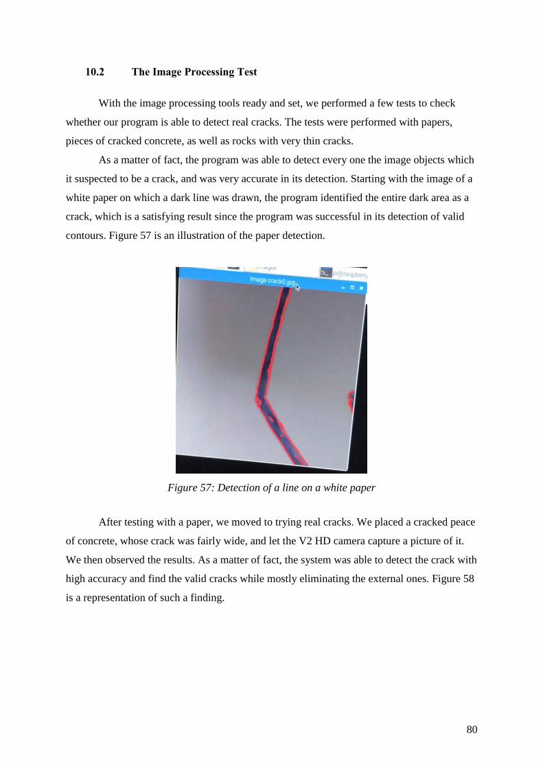
80
10.2 The Image Processing Test
With the image processing tools ready and set, we performed a few tests to check
whether our program is able to detect real cracks. The tests were performed with papers,
pieces of cracked concrete, as well as rocks with very thin cracks.
As a matter of fact, the program was able to detect every one the image objects which
it suspected to be a crack, and was very accurate in its detection. Starting with the image of a
white paper on which a dark line was drawn, the program identified the entire dark area as a
crack, which is a satisfying result since the program was successful in its detection of valid
contours. Figure 57 is an illustration of the paper detection.
Figure 57: Detection of a line on a white paper
After testing with a paper, we moved to trying real cracks. We placed a cracked peace
of concrete, whose crack was fairly wide, and let the V2 HD camera capture a picture of it.
We then observed the results. As a matter of fact, the system was able to detect the crack with
high accuracy and find the valid cracks while mostly eliminating the external ones. Figure 58
is a representation of such a finding.
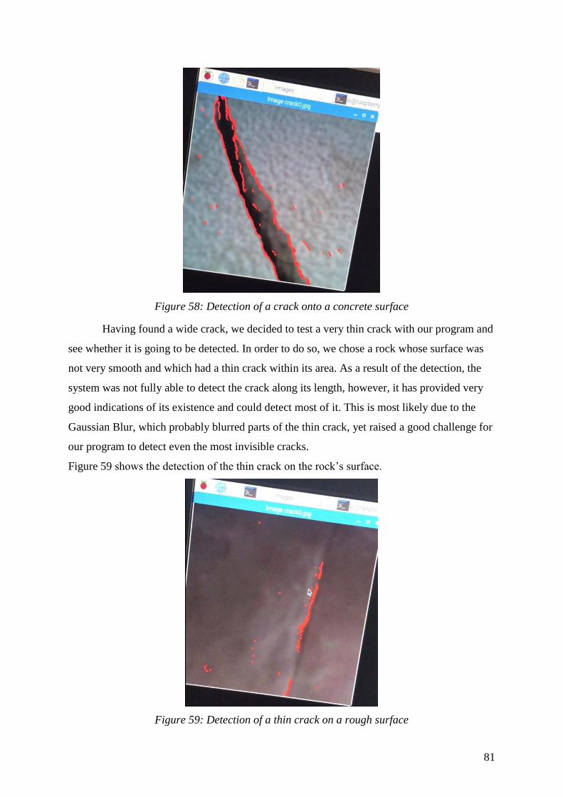
81
Figure 58: Detection of a crack onto a concrete surface
Having found a wide crack, we decided to test a very thin crack with our program and
see whether it is going to be detected. In order to do so, we chose a rock whose surface was
not very smooth and which had a thin crack within its area. As a result of the detection, the
system was not fully able to detect the crack along its length, however, it has provided very
good indications of its existence and could detect most of it. This is most likely due to the
Gaussian Blur, which probably blurred parts of the thin crack, yet raised a good challenge for
our program to detect even the most invisible cracks.
Figure 59 shows the detection of the thin crack on the rock’s surface.
Figure 59: Detection of a thin crack on a rough surface
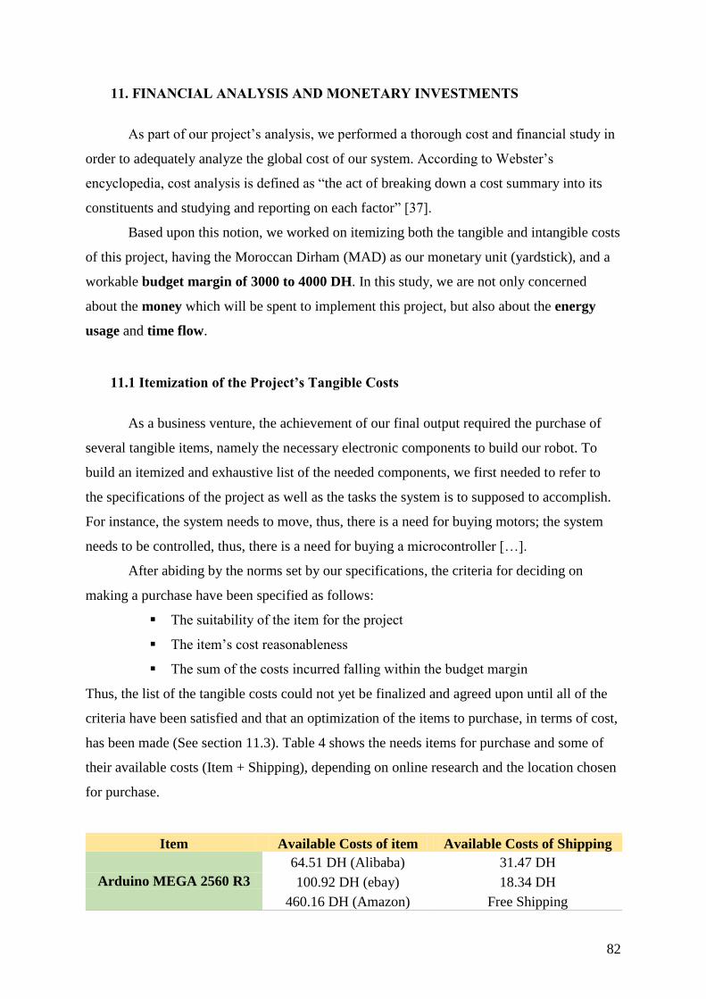
82
11. FINANCIAL ANALYSIS AND MONETARY INVESTMENTS
As part of our project’s analysis, we performed a thorough cost and financial study in
order to adequately analyze the global cost of our system. According to Webster’s
encyclopedia, cost analysis is defined as “the act of breaking down a cost summary into its
constituents and studying and reporting on each factor” [37].
Based upon this notion, we worked on itemizing both the tangible and intangible costs
of this project, having the Moroccan Dirham (MAD) as our monetary unit (yardstick), and a
workable budget margin of 3000 to 4000 DH. In this study, we are not only concerned
about the money which will be spent to implement this project, but also about the energy
usage and time flow.
11.1 Itemization of the Project’s Tangible Costs
As a business venture, the achievement of our final output required the purchase of
several tangible items, namely the necessary electronic components to build our robot. To
build an itemized and exhaustive list of the needed components, we first needed to refer to
the specifications of the project as well as the tasks the system is to supposed to accomplish.
For instance, the system needs to move, thus, there is a need for buying motors; the system
needs to be controlled, thus, there is a need for buying a microcontroller […].
After abiding by the norms set by our specifications, the criteria for deciding on
making a purchase have been specified as follows:
The suitability of the item for the project
The item’s cost reasonableness
The sum of the costs incurred falling within the budget margin
Thus, the list of the tangible costs could not yet be finalized and agreed upon until all of the
criteria have been satisfied and that an optimization of the items to purchase, in terms of cost,
has been made (See section 11.3). Table 4 shows the needs items for purchase and some of
their available costs (Item + Shipping), depending on online research and the location chosen
for purchase.
Item Available Costs of item Available Costs of Shipping
Arduino MEGA 2560 R3
64.51 DH (Alibaba) 31.47 DH
100.92 DH (ebay) 18.34 DH
460.16 DH (Amazon) Free Shipping

83
Raspberry Pi 3
405.42 DH (Banggood) Free Shipping
333.62 DH (Amazon) 42.03 DH
415.45 DH (The Pi Hut) Free Shipping
Raspberry Pi V2 HD
Camera
500 DH (Store in Fes) No Shipping
233.35 DH (Amazon) Free Shipping
601.81 DH (ebay) 20.66 DH
Hercules Dual Motor
Controller
267.27 DH (Seeed) 55.30 DH
322.56 DH (Amazon) Free Shipping
543.75 DH
(EPICTINKER) Free Shipping
Ultrasonic Sensors
3.69 DH (Alibaba) 5.04 DH
12.85 DH (ebay) Free Shipping
35.02 DH (Amazon) Free Shipping
Sharp Infrared Distance
Sensor
109.74 DH (Amazon) Free Shipping
110.59 (DFROBOT) Free Shipping
128.56 DH (sparkfun) 36.86 DH
LiPo Battery 7.4V
137.69 DH (GearBest) 47.09 DH
86.45 DH (ebay) 4.52 DH
562.09 DH (Gensace) 34.12 DH
Magnetic Encoder Pair 200 DH (Store in Fes) No Shipping
2.7 - 18V DC Motors 80 DH (Store in Fes) No Shipping
USB DC-DC Converter 25 DH (Store in Fes) No Shipping
ON-OFF Power Switch
17 DH (Store in
Casablanca) No Shipping
Wires 5 DH (Shop in Ifrane) No Shipping
Metal Frames 289 DH (Ingeniarius) 67 DH
Table 4: The tangible costs incurred by the project
Seen that the project has been achieved by one person, which involved the assembly,
wiring, mounting, and testing of the system, it can be affirmed that the project has no
operating or staffing costs. In addition, the utilities used have been provided by the
university and have not been paid for, thus not included in this tangible cost itemization.
11.2 Itemization of the Project’s Intangible Costs
In addition to the tangible costs and expenses, this project is also composed of
intangible demands. The latter involve the time, energy, as well as the established routine to
fully complete the project. Unlike a regular company where the intangible costs are
calculated in terms of money, i.e. how much money can be estimated for the time and energy
spent, we are going to give an estimation of the time elapsed from the start to the completion

84
of the project. Indeed, there is no money that could be made had the time not been spent on
this capstone, which makes the possibility for calculating time in terms of money improper.
This said, our yardstick in this section would be hours.
Given that the project was clearly agreed upon on January 17th, and that its
completion has not become final until April 4th, 77 days have flown by and are the working
period of the project. This said, the time expenditure can be formulized in terms of the
routine established during a week, its projection during a day, then finally the total time spent
in hours. Table 5 quantifies those intangible costs in numbers.
Weekly routine established 10 to 12 hours per week
Time projection during a day 1.43 to 1.71 hours per day
Total time spent on the project Between 110 and 132 hours
Table 5: The intangible costs incurred by the project
11.3 Expenditure Optimization and Weighted Decision Matrix
As previously determined, the budget assigned for the achievement of this project
ranges between 3000 and 4000 DH. Therefore, it is necessary to optimize the expenditure of
such a budget, in order not to exceed the margin and guarantee its efficient use.
In this section, we are going to refer back to the tangible costs of the project with the
intent to choose the most suitable and most convenient for our project, in terms of both cost
and quality.
Based upon this reasoning, a decision matrix has been developed in order to make
final decision about the items to purchase. The latter took into consideration their quality, as
well as the prices of both purchase and shipping. For every item, every criterion (Quality –
Price – Shipping) is going to be assigned a weight from 1 to 9, where 1 is an indication of
“Very inadequate”, 9 being “Very adequate”, and the more the numbers increase (between
1 and 9), they indicate that the quality/price/shipping of the item is “More adequate”. Table
6 represents the weighted decision matrix, which justifies our choice of the items found on
the internet. The items whose ‘Total’ is labeled in green were the ones purchased.
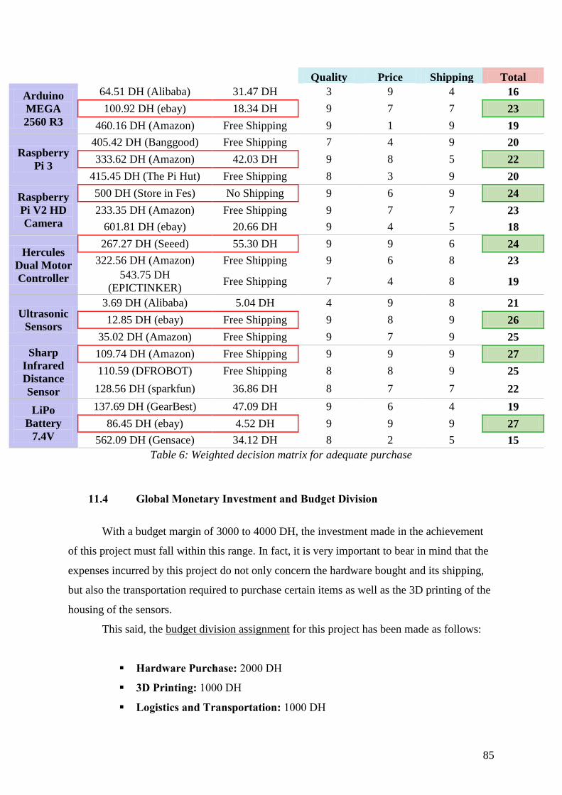
85
Quality Price Shipping Total
Arduino
MEGA
2560 R3
64.51 DH (Alibaba) 31.47 DH 3 9 4 16
100.92 DH (ebay) 18.34 DH 9 7 7 23
460.16 DH (Amazon) Free Shipping 9 1 9 19
Raspberry
Pi 3
405.42 DH (Banggood) Free Shipping 7 4 9 20
333.62 DH (Amazon) 42.03 DH 9 8 5 22
415.45 DH (The Pi Hut) Free Shipping 8 3 9 20
Raspberry
Pi V2 HD
Camera
500 DH (Store in Fes) No Shipping 9 6 9 24
233.35 DH (Amazon) Free Shipping 9 7 7 23
601.81 DH (ebay) 20.66 DH 9 4 5 18
Hercules
Dual Motor
Controller
267.27 DH (Seeed) 55.30 DH 9 9 6 24
322.56 DH (Amazon) Free Shipping 9 6 8 23
543.75 DH
(EPICTINKER) Free Shipping 7 4 8 19
Ultrasonic
Sensors
3.69 DH (Alibaba) 5.04 DH 4 9 8 21
12.85 DH (ebay) Free Shipping 9 8 9 26
35.02 DH (Amazon) Free Shipping 9 7 9 25
Sharp
Infrared
Distance
Sensor
109.74 DH (Amazon) Free Shipping 9 9 9 27
110.59 (DFROBOT) Free Shipping 8 8 9 25
128.56 DH (sparkfun) 36.86 DH 8 7 7 22
LiPo
Battery
7.4V
137.69 DH (GearBest) 47.09 DH 9 6 4 19
86.45 DH (ebay) 4.52 DH 9 9 9 27
562.09 DH (Gensace) 34.12 DH 8 2 5 15
Table 6: Weighted decision matrix for adequate purchase
11.4 Global Monetary Investment and Budget Division
With a budget margin of 3000 to 4000 DH, the investment made in the achievement
of this project must fall within this range. In fact, it is very important to bear in mind that the
expenses incurred by this project do not only concern the hardware bought and its shipping,
but also the transportation required to purchase certain items as well as the 3D printing of the
housing of the sensors.
This said, the budget division assignment for this project has been made as follows:
Hardware Purchase: 2000 DH
3D Printing: 1000 DH
Logistics and Transportation: 1000 DH
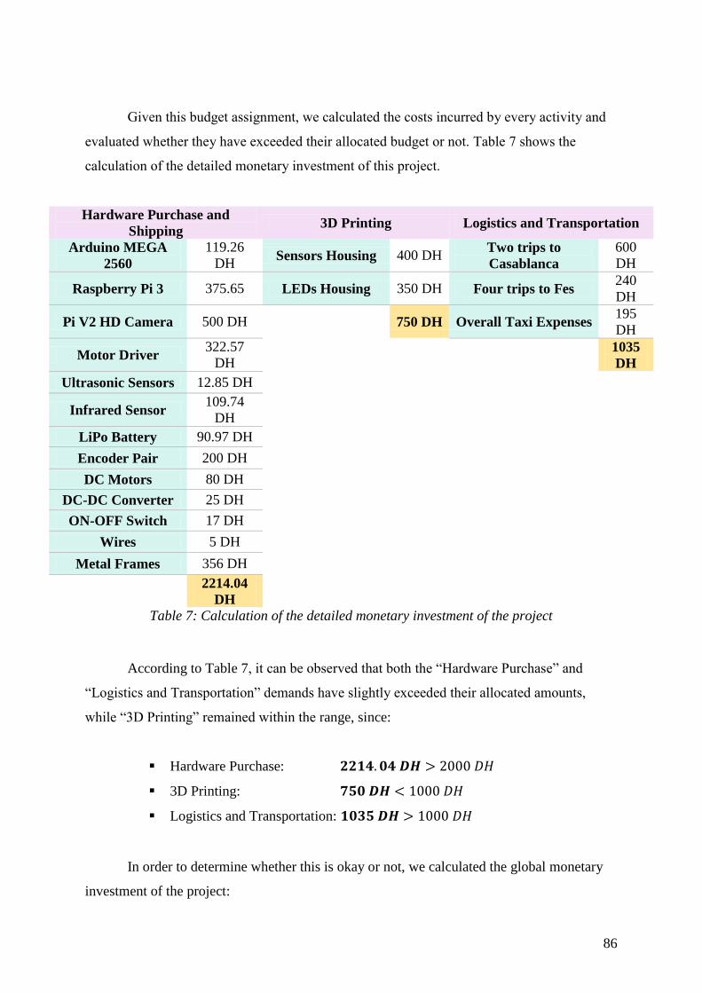
86
Given this budget assignment, we calculated the costs incurred by every activity and
evaluated whether they have exceeded their allocated budget or not. Table 7 shows the
calculation of the detailed monetary investment of this project.
Hardware Purchase and
Shipping 3D Printing Logistics and Transportation
Arduino MEGA
2560
119.26
DH Sensors Housing 400 DH
Two trips to
Casablanca
600
DH
Raspberry Pi 3 375.65 LEDs Housing 350 DH Four trips to Fes 240
DH
Pi V2 HD Camera 500 DH 750 DH Overall Taxi Expenses 195
DH
Motor Driver 322.57
DH
1035
DH
Ultrasonic Sensors 12.85 DH
Infrared Sensor 109.74
DH
LiPo Battery 90.97 DH
Encoder Pair 200 DH
DC Motors 80 DH
DC-DC Converter 25 DH
ON-OFF Switch 17 DH
Wires 5 DH
Metal Frames 356 DH
2214.04
DH
Table 7: Calculation of the detailed monetary investment of the project
According to Table 7, it can be observed that both the “Hardware Purchase” and
“Logistics and Transportation” demands have slightly exceeded their allocated amounts,
while “3D Printing” remained within the range, since:
Hardware Purchase: 𝟐𝟐𝟏𝟒. 𝟎𝟒 𝑫𝑯 > 2000 𝐷𝐻
3D Printing: 𝟕𝟓𝟎 𝑫𝑯 < 1000 𝐷𝐻
Logistics and Transportation: 𝟏𝟎𝟑𝟓 𝑫𝑯 > 1000 𝐷𝐻
In order to determine whether this is okay or not, we calculated the global monetary
investment of the project:

87
𝑮𝒍𝒐𝒃𝒂𝒍 𝑴𝒐𝒏𝒆𝒕𝒂𝒓𝒚 𝑰𝒏𝒗𝒆𝒔𝒕𝒎𝒆𝒏𝒕 = 2214.04 + 750 + 1035 = 𝟑𝟗𝟗𝟗. 𝟎𝟒 𝑫𝑯
Since 𝟑𝟗𝟗𝟗. 𝟎𝟒 𝑫𝑯 < 𝟒𝟎𝟎𝟎 𝑫𝑯, we have been successfully able to stay within our
expenditure margin and not exceed our budget. Although both the hardware purchase and
transportation activities exceeded their allocated amount, the remainder of the 3D printing
activity could compensate for that, given that it remained lower than its assigned value.
This project was achieved with a global investment of ≈ 𝟒𝟎𝟎𝟎 𝑫𝑯, thus, our budgeting
division decisions could be judged adequate.

88
12. CRACK DETECTION IN MOROCCO – INTERVIEWS
With the intent to enrich our study and broaden its scope, it was substantial to inquire
about the methods of crack detection currently employed in Morocco, as a centered focus on
the methods previously enumerated in the literature review. In order to do so, we selected a
few questions we judged are important for the study and listed them in a questionnaire for the
technical teams to answer.
12.1 Crack Detection Methods at Al Akhawayn University’s Ground and
Maintenance Department, Ifrane
In order to investigate about the employed crack detection methods in Morocco, we
started by our surrounding environment, which is Al Akhawayn University. Knowing that the
university’s Ground and Maintenance Department is responsible for all pipeline conduction
and maintenance, we contacted Mr. Mohamed Zaki, a technician in the department, who
provided us with all the information we needed.
Q. Is crack detection inside pipes a demanding process to follow?
A. Many times, it is. However, unless we notice actual leakage from the pipe, the crack
is not to worry about.
Q. What are the most common methods to detect a crack?
A. We usually detect cracks through technical inspection as the technical team examines
the pipes, and sees where pressure might drop abruptly, but besides, we use a special
camera.
Q. Do you use any technologies or devices for crack detection?
A. Yes, this is the camera I told you about. The device is composed of a long wire which
is entered along the pipe and on which a camera is mounted. Thanks to the screen
which is linked to the other tip of the wire, we can see anything that is inside the pipe,
whether there were cracks or residuals blocking the liquid’s way.
(See the device on Figure 60)
Q. How accurate is crack detection using your current technology?
A. Well, we can only see the inside of the pipe. The device does not really do much but
that. However, many times, we were able to spot developing cracks which were going
to entail unwanted consequences.
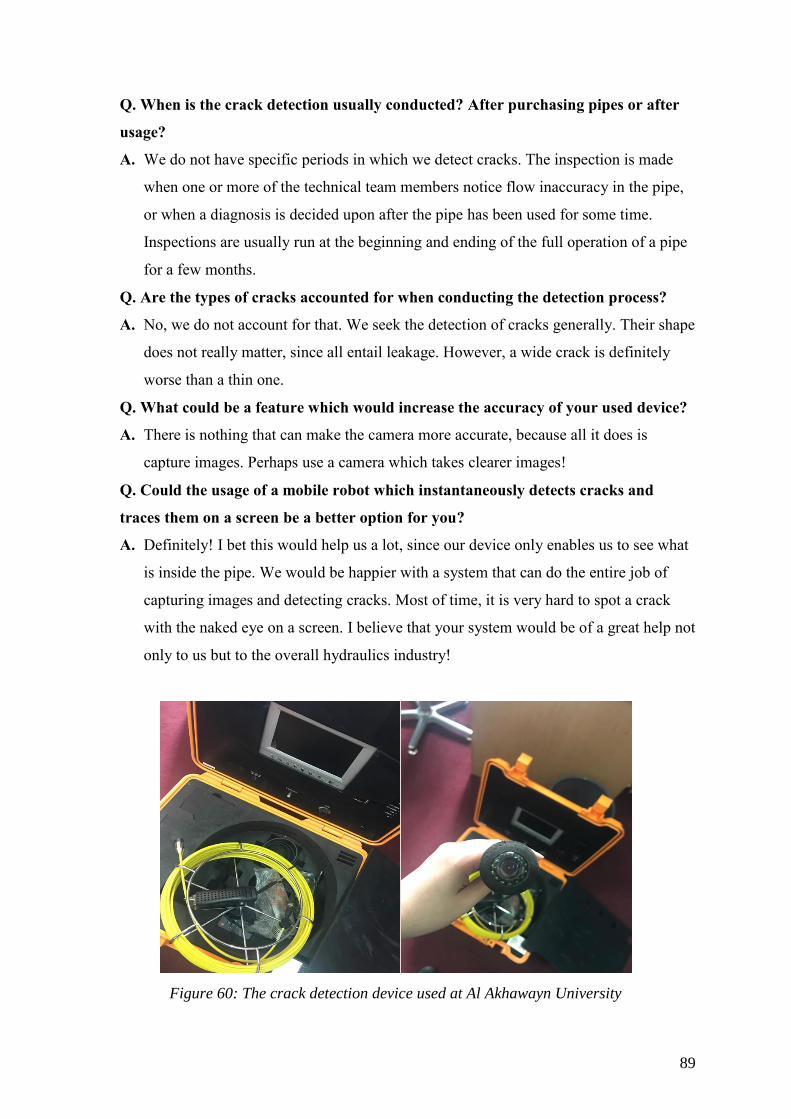
89
Q. When is the crack detection usually conducted? After purchasing pipes or after
usage?
A. We do not have specific periods in which we detect cracks. The inspection is made
when one or more of the technical team members notice flow inaccuracy in the pipe,
or when a diagnosis is decided upon after the pipe has been used for some time.
Inspections are usually run at the beginning and ending of the full operation of a pipe
for a few months.
Q. Are the types of cracks accounted for when conducting the detection process?
A. No, we do not account for that. We seek the detection of cracks generally. Their shape
does not really matter, since all entail leakage. However, a wide crack is definitely
worse than a thin one.
Q. What could be a feature which would increase the accuracy of your used device?
A. There is nothing that can make the camera more accurate, because all it does is
capture images. Perhaps use a camera which takes clearer images!
Q. Could the usage of a mobile robot which instantaneously detects cracks and
traces them on a screen be a better option for you?
A. Definitely! I bet this would help us a lot, since our device only enables us to see what
is inside the pipe. We would be happier with a system that can do the entire job of
capturing images and detecting cracks. Most of time, it is very hard to spot a crack
with the naked eye on a screen. I believe that your system would be of a great help not
only to us but to the overall hydraulics industry!
Figure 60: The crack detection device used at Al Akhawayn University
90
12.2 Crack Detection Methods at RADEEMA, Marrakech
Being a leader in the Moroccan public sector of water conduction and distribution,
RADEEMA is a utility operator that manages the distribution of water and electricity, as well
as the collection of wastewater and rainwater in the city of Marrakech. Among its main tasks
are the following:
Drinking water distribution
Liquid sanitation management (wastewater and rainwater)
Electricity distribution
Public lighting management
As part of our investigation of the existence of cracks inside industrial pipes, we
interviewed Mr. Zakaria Benharref, a hydraulics engineer at RADEEMA, Marrakech, and
asked him a few questions related to the technologies employed to spot pipeline crack.
The interview went on as follows:
Q. Is crack detection inside pipes a demanding process to follow?
A. Well, relatively. Sometimes, it is very hard to spot a crack without manual
verification when devices do not provide us with accurate results. It usually takes
someone to do pressure tests to check whether the crack is actually there. And in fact,
those could be very dangerous, aside from the fact they produce leakage. When they
create a huge pressure difference between the inside of the pipe and the outside
environment, the pipe would eventually explode.
Q. What are the most common methods to detect a crack?
A. The most used way to detect cracks is the “pressure control” method. It is based on
measuring pressure along the pipe, until a decrease in pressure is noticed. This,
indeed, means that there is a leakage of air at that specific spot, which makes it easier
to determine the existence of a crack. However, the simplest way to detect cracks is
just to put the entire pipe subject to technical diagnosis where it is fully examined and
tested. In the past, there were some industrial clients who had spotted cracks in our
pipes for us to repair.
Q. Do you use any technologies or devices for crack detection?
A. The use of electronic devices to detect cracks is not called for unless the pressure test
fails to unveil a crack. However, we use adjustable amplifiers and frequency filters,
which work with “acoustic correlation”. The concept of this method is pretty simple:
91
In two accessible points of a pipe, we collect the noise emitted by a leak as well as the
time it lags compared to a “normal signal”. The identified noise emitted at an instant t,
will arrive with a certain time lag from point A compared to point B. In fact, since we
are able to quantify this time lag ∆𝑡 and know the speed of sound, we can easy locate
the origin of the noise, which must be a crack.
Q. How accurate is crack detection using your current technology?
A. The acoustic correlation? Well, mostly accurate, however there were a lot of times
where false signals were emitted. We usually send someone along the pipe to the spot
where the device indicated the existence of a crack to examine it, and confirm using
the pressure test. It is hard to trust electronic devices only, as the replacement of a
pipe is not easy job and may cause an interruption while the pipe is being repaired or
replaced.
Q. When is the crack detection usually conducted? After purchasing pipes or after
usage?
A. As the pipes are purchased from the manufacturer, the technical team at RADEEMA
examines their aptitude and puts them subject to minute diagnosis. Of course, there
always are defects in the material we purchase from other companies. However, we
do not usually perform any other tests on the pipes unless we suspect there might be a
leakage somewhere during operation. Therefore, the crack detection methods that I
talked about are usually employed after the pipes have been used for some time and
that we suspect there might be a crack somewhere due to leakage or the decrease of
internal pressure.
Q. Are the types of cracks accounted for when conducting the detection process?
A. Relatively. If you are referring to the types of cracks as in transverse or longitudinal
ones, we are not really concerned about the crack’s shape or its orientation. However,
what really matters to us is the depth of the crack and its width. The deeper the crack,
the easier it is for the conducted liquid to leak, and the wider it is, the higher the
leakage flow. Using our pressure test, a sudden decrease in internal pressure would
indicate a wide crack, and using the acoustic test, a sharp signal would indicate a deep
crack.
Q. What could be a feature which would increase the accuracy of your acoustic
device?
A. We would be happy with a more precise device, since the one we are currently
employing is not very exact as I mentioned before. There should always be somebody

92
checking after the device and confirming the existence or non-existence of a crack
with the pressure test. We would be glad if there was a system which can come up
with a more accurate result, and unveil the crack to us without further detection.
Q. Could the usage of a mobile robot which instantaneously detects cracks and
traces them on a screen be a better option for you?
A. This sounds like a brilliant idea. We would be more than happy to have this device, as
we will have the crack detected and also be able to see it. Having it traced on a screen
would not only provide us with information about its shape and width, but would also
reduce the workforce used as the technicians would not have to recheck after the
detection device. I think this would be really great to implement. The industry is very
much in need of devices like this one. I suppose that there are cameras which take
pictures along the pipe, but they perhaps cannot spot the cracks themselves. This
device would make our lives easier!
93
13. SYSTEM ADVANTAGES AND LIMITATIONS
Just like every system, the mobile robot developed and studied in this project has got
its own advantages and limitations. Indeed, it goes without saying that the task of performing
image processing with a moving system raises a lot of concerns and matters to thoroughly
account for. We attempted to classify those as advantages or limitations, following the
system’s achievements as well as the challenges which were faced during this study.
13.1 System Advantages
During the robot’s testing and operation, we were able to record several achievements
attained by our system. As shown previously, we were able to calibrate the camera in such a
way that the robot takes images at a time lapse convenient for its speed, and proportional to
both the pipe’s length and diameter. Additionally, the crack detection performed by our
developed program has proven good accuracy with both visible and thin-hair cracks. Besides,
we were able to have our system remotely move inside a pipe, after the Arduino sketch
(code) has been uploaded on the Arduino board. This enabled us to continuously track our
robot’s position using either the output returned by the encoders or a simple computation of
the system’s traversed distance with a known distance and time lapse.
13.2 System Limitations
This project was also faced with a few limitations which need to be pointed out and
considered. It goes without saying that the Raspberry Pi, as a mini-computer, needs to be
uninterruptedly powered during operation. While the latter is not equipped with an on-off
switch, this design constraint has put us faced with the challenge of having the Raspberry Pi
constantly wired to a power source, hence the entire robot as it moves. Besides, as we are
working with a microcontroller uniquely responsible for the motion and sensors of the robot
and that the images are being captured by the Raspberry Pi, it is not yet possible to stop the
robot at a precise position and ask it to take an image at a specific time. The camera is also
placed on top of the robot, thus, it only captures images of the upper wall of the pipe.
94
14. HONORS PROGRAM REQUIREMENT
14.1 Environmental Impact
Given that our study suggests a mechatronic system for crack detection, its implications
are strictly not pollutant nor harmful for the environment. We proposed an environmentally
friendly system which is sustainable unique in its design. This said, we have provided an
alternative for the chemical approaches used to detect cracks inside pipe lines, such as the
chemical dye method to unveil cracks. With zero emissions nor chemical use, our system is
then ideal for usage in engineering applications, specifically those related to area or tunnel
investigation, in addition to crack detection or broadly the detection of objects.
14.2 Ethical Considerations
On the one hand, we showed ethical consideration to the environment through
contributing in the prevention of engineering disasters, which could cause tremendous harm.
Also, we made sure to deliver a fully reliable prototype by performing a number of reliability
tests inside real pipes, while recording observations for repair and future improvements. On
the other hand, we made sure we adhered to the academic integrity implied by the university,
and conveyed feedback about the advancement of our project throughout its realization. We
also ensured the originality of this work and that it embodies a variety of concepts thoroughly
tackled and utilized.
14.3 Research and Multidisciplinarity
Seen the manifold topic of crack detection, research was essentially maintained
throughout this project starting from the literature review to inquire about the types of cracks
used in industry, to other topics touching on the core of this capstone. Before tackling motion
and kinematics, we conducted research in order to grasp the concept of differential drive
along with its sub-notions such as the Instantaneous Center of Curvature. Concerning control,
research was necessary in order to inquire about control theory in classical mathematics, in
addition to PID Control and its components. Regarding software management, we thoroughly
researched about the list of commands to follow in order to install both the Raspbian Stretch
95
and OpenCV. Likewise, extensive research was also made to look into feature detection as
well as the different crack detection algorithms found in the literature.
Besides, this project is judged multidisciplinary, seen the many disciplines it invites in
and crisscrosses. First, the functional architecture of our robot relies on the connections of
electronic hardware with, as a basis, corresponding knowledge in electric circuits. In what
concerns chassis assembly and mounting, a few skills in mechanics were also needed,
without neglecting the CAD design which necessitated knowledge in mechanical modeling.
Coming to the algorithmic side of this project, mathematics was constantly called upon in
order to understand mathematical concepts such as Sobel gradients, and be able to write
programs, thus employ knowledge in computer programming. Additionally, this project
comprised a financial study, which also makes it touch on the realm of finance, without
forgetting interviews with Moroccan engineers and technicians, which brought in a social
sciences component.
96
15. STEEPLE Analysis
While considering the crack detection issue within transportation pipes’ industries,
several regards arise and prove the necessity of accounting for significant aspects during the
design and implementation of a technologically innovative crack detection system. The latter
view the problem from distinct angles, and render the proposed solution’s objectives from
said perspectives.
Socially, this project aims at decreasing laborious effort when it comes to crack
detection, through proposing an effort-efficient system to facilitate the job for technical
maintenance teams at distribution stations. Additionally, it seeks to promote the usage of
sophisticated technologies within Moroccan industries, instead of the traditional ones which
are time consuming. This all would contribute in raising awareness with regards to the urgent
detection of cracks inside pipes in a timelier manner, before the latter enlarge and cause
major engineering disasters.
Technologically, this project is a great mean for designing and building an efficient
and innovative crack detection system, which brings all pertinent disciplines to collaborate.
Firstly, the system’s functioning relies on the usage of electronic hardware as well as
knowledge in electrical engineering for a successful internal architecture. Second, it relies for
its control, on computer science, seen the used kinematics programs and control algorithms,
in addition to computer vision technology. Third, the system requires skills in mechanical
engineering, such as mounting and soldering, to ensure its full assembly and operational use.
And finally, the precise edge detection algorithms which are based on gradients and
significant mathematical and geometrical formulas call upon applied mathematics as a major
discipline present throughout the project’s preparation.
Environmentally, the project promotes the usage of an environmentally friendly
system for crack detection, which will not pollute or harm the environment. In contrast to
some systems found in the literature and which use chemical substances to unveil cracks, this
system can spot their existence with more precision and without the use of any
environmentally harmful chemicals. This comes as a great promotion for the employment of
green electronics in maintenance operations, in order to avoid deleterious emissions and
negatively impact the environment.
Ethically, the proposed system will contribute in the prevention of major engineering
disasters, like the leakage of toxic substances to the environment, which may cause
irreparable disasters and permanently harm the environment. It is also important to test the
97
reliability of this self-made prototype, in order to present it as a fully operational system for
Moroccan industries. This will not only improve the quality of crack detection in industries,
but will also help take part of global action towards protecting the environment, while using
pertinent scientific and technological means.
Politically, this project proposes a locally-made technological system, and promotes
the beginning of a reduced trend in importing foreign and external technological imports. It
also helps elevate and boost significant political action against environmentally harmful
means for crack detection. By doing so, the system will present itself as a candidate to be a
governmentally approved system for use within Moroccan industries, especially those in
which engineering disasters are the most likely to happen, such as in the marine industry
where merchant vessels are used for petroleum transportation inside industrial pipes.
Legally, one of the main objectives is to help industries respect the legal
considerations of safe sewage conductions, notably those which deal with delicate
engineering substances. Also, the system is to ensure a thorough respect of the rules and
regulations of substance transportation and distribution, be it to houses or industries, so as to
avoid the legal implications of the violation which could occur due to failure in accurately
detecting cracks inside transportation pipes.
Economically, this project aims at providing cheaper alternatives for expensive crack
detection technologies and imports, such as vibration devices which are highly expensive and
may require maintenance. Furthermore, this is to suggest an economic system, whose
constituting parts are widely available within the Moroccan market, at local electronics’
providers for cheaper prices than those imported. And as an additionally economical concern,
it is crucial to study consumers’ attitudes and behavior, in addition to their satisfaction with
regards to the proposed technology, so as to improve its features and provide more
satisfactory boosts and enhancements.
Figure 61 is a summary of the STEEPLE analysis.
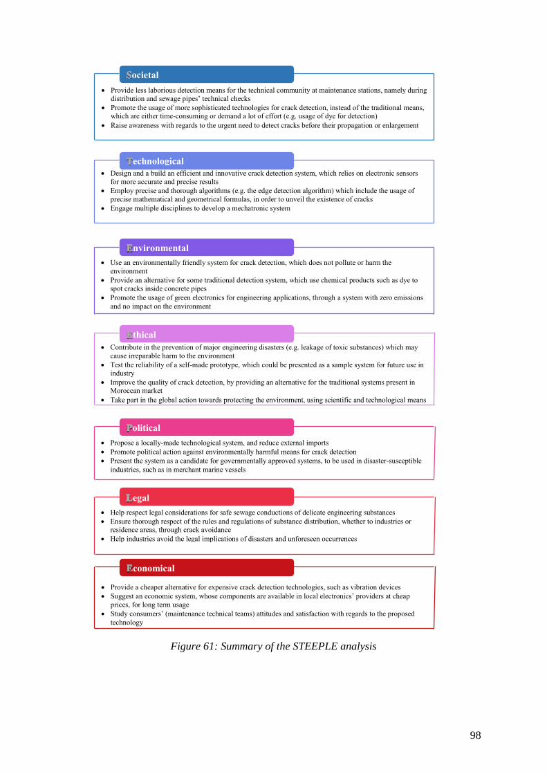
98
Figure 61: Summary of the STEEPLE analysis
Provide a cheaper alternative for expensive crack detection technologies, such as vibration devices
Suggest an economic system, whose components are available in local electronics’ providers at cheap
prices, for long term usage
Study consumers’ (maintenance technical teams) attitudes and satisfaction with regards to the proposed
technology
Provide less laborious detection means for the technical community at maintenance stations, namely during distribution and sewage pipes’ technical checks
Promote the usage of more sophisticated technologies for crack detection, instead of the traditional means, which are either time-consuming or demand a lot of effort (e.g. usage of dye for detection)
Raise awareness with regards to the urgent need to detect cracks before their propagation or enlargement
ocietal
Design and a build an efficient and innovative crack detection system, which relies on electronic sensors
for more accurate and precise results
Employ precise and thorough algorithms (e.g. the edge detection algorithm) which include the usage of
precise mathematical and geometrical formulas, in order to unveil the existence of cracks
Engage multiple disciplines to develop a mechatronic system
echnological
conomical
Use an environmentally friendly system for crack detection, which does not pollute or harm the
environment
Provide an alternative for some traditional detection system, which use chemical products such as dye to spot cracks inside concrete pipes
Promote the usage of green electronics for engineering applications, through a system with zero emissions
and no impact on the environment
nvironmental
Contribute in the prevention of major engineering disasters (e.g. leakage of toxic substances) which may
cause irreparable harm to the environment
Test the reliability of a self-made prototype, which could be presented as a sample system for future use in industry
Improve the quality of crack detection, by providing an alternative for the traditional systems present in Moroccan market
Take part in the global action towards protecting the environment, using scientific and technological means
thical
Propose a locally-made technological system, and reduce external imports
Promote political action against environmentally harmful means for crack detection
Present the system as a candidate for governmentally approved systems, to be used in disaster-susceptible
industries, such as in merchant marine vessels
olitical
Help respect legal considerations for safe sewage conductions of delicate engineering substances
Ensure thorough respect of the rules and regulations of substance distribution, whether to industries or residence areas, through crack avoidance
Help industries avoid the legal implications of disasters and unforeseen occurrences
egal

99
16. CONCLUSION AND FUTURE WORK
The principal goal of this capstone was to build a working prototype of a mechatronic
system able to move and traverse pipes, as it captures images, analyses them, and unveils
whether a crack exists or not. With our specifications set and agreed upon, we first worked on
choosing the adequate pieces of hardware to build the system, and established its main
connections and internal architecture. The assembly and mounting included the wiring of the
main printed circuit boards, sensors and actuators’ connections, in addition to the fixation of
metal frames and the chassis using screws.
After doing so, we modeled a shell for our robot using FreeCAD, then began working
on its kinematics. Assuming that the robot only has to move forward, we developed an
algorithm which updates the position of the robot as well as makes it move in a linear trend.
We concluded that the angular velocity must be set to zero for the system, and that the
distance traversed must be calculated following the rotary encoders’ pulses per iteration.
In order to control our platform, it was necessary to pick a controlling unit and
employ it. Therefore, we chose to use the PID controller, the most famous control feedback
mechanism used in mechatronics applications. While using the latter, we concluded that the
proportional coefficient is mostly responsible for the wheels’ tilt, and that the integral and
derivative coefficients are respectively responsible for the wheels moving too slow or too
fast. Building on the robot’s overall control, we were also able to retrieve the sensors’
returned values and know the instant in which our robot exits a given pipe.
Coming to the computer vision part, we first had to configure our camera and link it
to the Raspbian Stretch, the Raspberry Pi’s operating system. We were, then, able to capture
images and store them in a known folder. However, we concluded that the camera must be
calibrated, as the robot is higher from the ground inside a pipe with a smaller diameter than it
is with one with a bigger diameter.
With the camera configured, we developed an image processing algorithm able to
accurately detect cracks and trace them. During the process, we concluded that the feature
detection to employ is edge detection, as cracks are mainly identified as edges and not as
points or blobs. We also concluded that the noise in the captured images must be reduced
through cropping their sides and corners using an offset of 185 pixels, and that techniques
such as image resizing or increasing the contrast ratio distort pixels’ distribution and alter the
original captured images.

100
The future work of this project would be centered around the synchronization of the
Arduino and the Raspberry Pi, in order to establish a communication cycle between the
system’s microcontroller and processor. This cycle is called a rosserial, which is cyclic
communication in which both members publish (send) data to one another and subscribe
(receive) to the other pieces of information acquired. A publisher is also called a talker, while
a subscriber is also named a listener. In our case, the Arduino would be sending the
position’s update and sensors’ output to the Raspberry Pi, while the later would be sending
the captured and analyzed images, so that the robot knows when to stop as a crack gets
detected at a location x. Additionally, extending the camera’s field of view to 360 degrees is
also part of our future work, using one of several solutions, such as a rod being rotated by a
DC motor and steadily turning the camera lens to cover a 360 degrees angle.
By the closure of this report, we would like to express how of much of an amazing
journey the realization of this project has been, throughout its different phases. It is with
utmost gratitude that we express our thankfulness to the people acknowledged at the
beginning of this report for their continuous support and collaboration, because hadn’t it been
for their help, this project would not have come to life.
We were, indeed, faced with numerous barriers which we eventually overcame and
surpassed, and are satisfied with the achievements our system was able to accomplish. We
hope that this journey, with its successes and hurdles, would be a path paving and
encouraging experience for hands-on prototype realization for the generations to come, as
well as a further step for more fruitful findings at the School of Science and Engineering.
101
17. BIBLIOGRAPHY
[1] “Resources Ultrasonic Flaw Detection,” An Introduction to Ultrasonic Flaw
Detection. [Online]. Available: https://www.olympus-ims.com/en/applications-and-
solutions/introductory-ultrasonics/introduction-flaw-detection/. [Accessed: 13-Apr-
2018].
[2] “Register now for our upcoming Webinar,” Ultrasonic in Line Inspection Company.
[Online]. Available: https://www.ndt-global.com/. [Accessed: 13-Apr-2018].
[3] Jiya, Anwar, N. S. N., Abdullah, and M. Z., “Detection of Cracks in Concrete
Structure Using Microwave Imaging Technique,” International Journal of Microwave
Science and Technology, 19-Jun-2016. [Online]. Available:
https://www.hindawi.com/journals/ijmst/2016/3195716/. [Accessed: 13-Apr-2018].
[4] R. Zoughi and S. Kharkovsky, “Microwave and Millimetre Wave Sensors for Crack
Detection,” Fatigue & Fracture of Engineering Materials & Structures, 2008.
[5] “Liquid Penetrant Testing - Hashemite University.” [Online]. Available:
https://www.bing.com/cr?IG=6F9070CF15E440598C01A0E9C7FF56B5&CID=38C
355A6FD8A67B820CD5E76FC2566F6&rd=1&h=N6FECJ6XQxDR1VBiws6j9batP
Gl-P9mIu1XOx2C3qO4&v=1&r=https://eis.hu.edu.jo/ACUploads/10526/Liquid
Penetrant Testing.pdf&p=DevEx,5062.1. [Accessed: 13-Apr-2018].
[6] M. A. Alam, M. M. N. Ali, M. A. A.-A. Syed, N. Sorif, and M. A. Rahaman, “An
algorithm to detect and identify defects of industrial pipes using image processing,”
The 8th International Conference on Software, Knowledge, Information Management
and Applications (SKIMA 2014), 2014.
[7] “Sika Group group,” Sika AG. [Online]. Available: https://www.sika.com/.
[Accessed: 13-Apr-2018].
[8] “Evaluating Cracking in Concrete - Bluey Technologies.” [Online]. Available:
http://www.bing.com/cr?IG=754DB61FF447488F9A0CAD44268FD898&CID=1105
2D11A07A6C722B9E26C1A1D56DDF&rd=1&h=YAZaY0_A2RJ_KJ9SoEUJst7Sa
GyJsdCB1dZdWoM7ebQ&v=1&r=http://www.bluey.com.au/wp-
content/uploads/2012/02/Cracking-in-Concrete-LR-R1.pdf&p=DevEx,5064.1.
[Accessed: 13-Apr-2018].
[9] Admin, “Different Types of Pipes and Tips for Choosing the Right One,” Bernardi
Building Supply - Service Built Our Business, 06-Dec-2017. [Online]. Available:
102
https://bernardibuildingsupply.com/pipe-supplies-toronto/different-types-of-pipes-
and-tips-for-choosing-the-right-one/. [Accessed: 13-Apr-2018].
[10] “Introduction to Mobile Robotics - unibo.it.” [Online]. Available:
http://www.bing.com/cr?IG=1203066306634903847578E05AFC83FA&CID=07B2B
EF619F56E983C88B526185A6F1A&rd=1&h=xnKYQ5PNCkYt7QOMD9YIxeQ3W
T8Qq-Y6Outp0OmG3Xw&v=1&r=http://www-
lar.deis.unibo.it/people/rfalconi/Mobile_robotics_ENG_NO_VIDEO.pdf&p=DevEx,5
067.1. [Accessed: 13-Apr-2018].
[11] Lima, P., Mobile Robotics, 2002.
[12] “Robotics/Introduction,” Robotics/Introduction - Wikibooks, open books for an open
world. [Online]. Available: https://en.wikibooks.org/wiki/Robotics/Introduction.
[Accessed: 13-Apr-2018].
[13] Couceiro, M., Introduction to Robotics, July 2017.
[14] Introduction to Robots. [Online]. Available:
http://www.galileo.org/robotics/intro.html. [Accessed: 13-Apr-2018].
[15] G. Anbarjafari, “1. Introduction to image processing,” Sisu@UT. [Online].
Available: https://sisu.ut.ee/imageprocessing/book/1. [Accessed: 13-Apr-2018].
[16] M. Rabbani, Fundamentals of digital image processing Sunday, May 21, 1995,
Dolphin Hotel, Orlando, Florida. Playa del Rey, CA: Society for Infoermation
Display, 1995.
[17] “Functional Architecture,” AcqNotes. [Online]. Available:
http://acqnotes.com/acqnote/careerfields/functional-architecture. [Accessed: 14-Apr-
2018].
[18] T. E. of E. Britannica, “Kinematics,” Encyclopædia Britannica, 21-Jun-2017.
[Online]. Available: https://www.britannica.com/science/kinematics. [Accessed: 14-
Apr-2018].
[19] Kozlowski Krzysztof, Robot motion and control 2011. London: Springer, 2012.
[20] “Inertial Frame of Reference: Definition & Example - Study.com.” [Online].
Available:
https://www.bing.com/cr?IG=1F22A1F263DD4FCF877D5C03CDC0DD46&CID=14
3D30997C986156106B3B487D37609A&rd=1&h=lkLjM_50D56ZtGficwCbHK6D
WqSuEtf8oOixpXvE5aE&v=1&r=https://study.com/academy/lesson/inertial-frame-
of-reference-definition-example-quiz.html&p=DevEx,5069.1. [Accessed: 14-Apr-
2018].

103
[21] Nature News. [Online]. Available: https://www.nature.com/subjects/control-theory.
[Accessed: 14-Apr-2018].
[22] “Chapter 1 - Introduction to Control Systems - Calvin College.” [Online]. Available:
http://www.bing.com/cr?IG=B1E936E376C0495B8E80AD4598896522&CID=315C
641A0BBB61B1015E6FCB0A146013&rd=1&h=xvrxGTPiW3bJVLlh4s3HXe0FZ6v
Xe_5Fq5g
0R0SqAo&v=1&r=http://www.calvin.edu/~pribeiro/courses/engr315/lectures-
notes/chapter-1.ppt&p=DevEx,5059.1. [Accessed: 14-Apr-2018].
[23] “What is the definition of a robot controller - Open Robotics.” [Online]. Available:
http://www.bing.com/cr?IG=94CA8E3AB3FD4FF2B74A890021E687C6&CID=2B9
95107D4876FE806475AD6D5286E8E&rd=1&h=jyzrpthrLC_AA1IVO9e_mmbVLF
gBy2YYM7jEGxdoE4g&v=1&r=http://open-robotics.com/what-is-the-definition-of-
a-robot-controller/?ckattempt=1&p=DevEx,5069.1. [Accessed: 14-Apr-2018].
[24] “PID controller - Wikipedia.” [Online]. Available:
https://www.bing.com/cr?IG=71CF725430A34833862C1A05C1694941&CID=1003
69C6A01664AD21066217A1B96561&rd=1&h=nFvqDIYvqA-
6VWN6q9R9b2U9anRIPn04NWTlYQeT-
GY&v=1&r=https://en.wikipedia.org/wiki/PID_controller&p=DevEx,5076.1.
[Accessed: 14-Apr-2018].
[25] “Rotary encoder - Wikipedia.” [Online]. Available:
https://www.bing.com/cr?IG=8E62B2B87A374EB4A3352DAC51D1688D&CID=34
24280CC2EE657A127923DDC3416451&rd=1&h=n6gnM_rSjSkcv_pPI--
6I38HNoC-
PtYrT27CY28cBaA&v=1&r=https://en.wikipedia.org/wiki/Rotary_encoder&p=DevE
x,5070.1. [Accessed: 14-Apr-2018].
[26] “Principles of Operation,” IR Sensor | What is an IR Sensor? [Online]. Available:
http://education.rec.ri.cmu.edu/content/electronics/boe/ir_sensor/1.html. [Accessed:
14-Apr-2018].
[27] “Raspberry Pi,” Wikipedia, 12-Apr-2018. [Online]. Available:
https://en.wikipedia.org/wiki/Raspberry_Pi. [Accessed: 14-Apr-2018].
[28] “Teach, Learn, and Make with Raspberry Pi,” Raspberry Pi. [Online]. Available:
https://www.raspberrypi.org/. [Accessed: 14-Apr-2018].
[29] “Python picamera,” Python picamera - Raspberry Pi Documentation. [Online].
Available:
104
https://www.raspberrypi.org/documentation/usage/camera/python/README.md.
[Accessed: 14-Apr-2018].
[30] “About,” About - OpenCV library. [Online]. Available:
https://opencv.org/about.html [Accessed: 14-Apr-2018].
[31] “Raspbian Stretch: Install OpenCV 3 Python on your Raspberry Pi,”
PyImageSearch,
16-Nov-2017. [Online]. Available:
https://www.pyimagesearch.com/2017/09/04/raspbian-stretch-install-opencv-3-
python-on-your-raspberry-pi/. [Accessed: 14-Apr-2018].
[32] M. A. Alam, M. M. N. Ali, M. A. A.-A. Syed, N. Sorif, and M. A. Rahaman, “An
algorithm to detect and identify defects of industrial pipes using image processing,”
The 8th International Conference on Software, Knowledge, Information Management
and Applications (SKIMA 2014), 2014.
[33] “What is gray scaling? Webopedia Definition.” [Online]. Available:
https://www.bing.com/cr?IG=B896CBAF05A3482D81C9ADD0B3AB7947&CID=2
6E71974784F6D441AA712A579E06C5F&rd=1&h=5QhaiTo0qFOQ5rvvJ9kXhRG
WKmbE-9-
H7zzYnPQcIA4&v=1&r=https://www.webopedia.com/TERM/G/gray_scaling.html&
p=DevEx,5067.1. [Accessed: 14-Apr-2018].
[34] “Feature detection (computer vision),” Wikipedia, 10-Apr-2018. [Online]. Available:
https://en.wikipedia.org/wiki/Feature_detection_(computer_vision). [Accessed: 14-
Apr-2018].
[35] “Edge Detection,” MATLAB & Simulink. [Online]. Available:
https://ch.mathworks.com/discovery/edge-detection.html. [Accessed: 14-Apr-2018].
[36] OpenCV: Image Denoising. [Online]. Available:
https://docs.opencv.org/3.3.1/d5/d69/tutorial_py_non_local_means.html. [Accessed:
14-Apr-2018].
[37] “Cost Analysis,” Merriam-Webster. [Online]. Available: https://www.merriam-
webster.com/dictionary/cost analysis. [Accessed: 14-Apr-2018].
[38] “Camera Module,” Camera Module - Raspberry Pi Documentation. [Online].
Available:
https://www.raspberrypi.org/documentation/hardware/camera/README.md.
[Accessed: 14-Apr-2018].
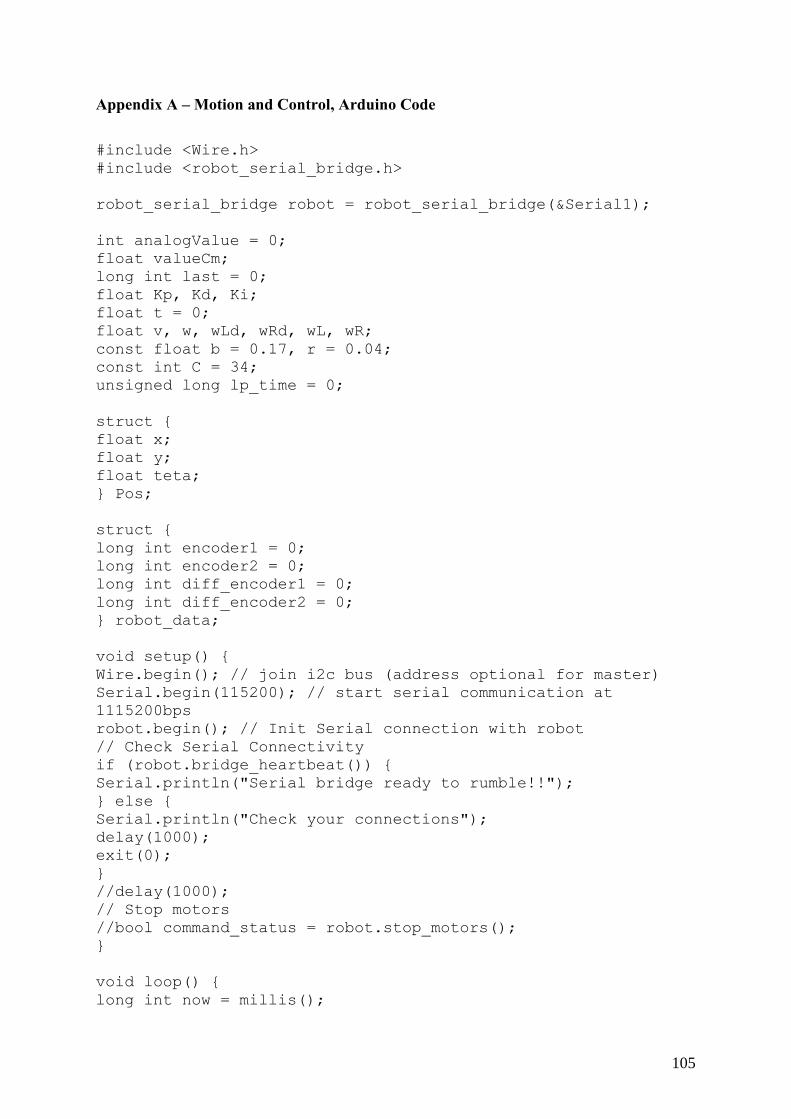
105
Appendix A – Motion and Control, Arduino Code
#include <Wire.h>
#include <robot_serial_bridge.h>
robot_serial_bridge robot = robot_serial_bridge(&Serial1);
int analogValue = 0;
float valueCm;
long int last = 0;
float Kp, Kd, Ki;
float t = 0;
float v, w, wLd, wRd, wL, wR;
const float b = 0.17, r = 0.04;
const int C = 34;
unsigned long lp_time = 0;
struct {
float x;
float y;
float teta;
} Pos;
struct {
long int encoder1 = 0;
long int encoder2 = 0;
long int diff_encoder1 = 0;
long int diff_encoder2 = 0;
} robot_data;
void setup() {
Wire.begin(); // join i2c bus (address optional for master)
Serial.begin(115200); // start serial communication at
1115200bps
robot.begin(); // Init Serial connection with robot
// Check Serial Connectivity
if (robot.bridge_heartbeat()) {
Serial.println("Serial bridge ready to rumble!!");
} else {
Serial.println("Check your connections");
delay(1000);
exit(0);
}
//delay(1000);
// Stop motors
//bool command_status = robot.stop_motors();
}
void loop() {
long int now = millis();
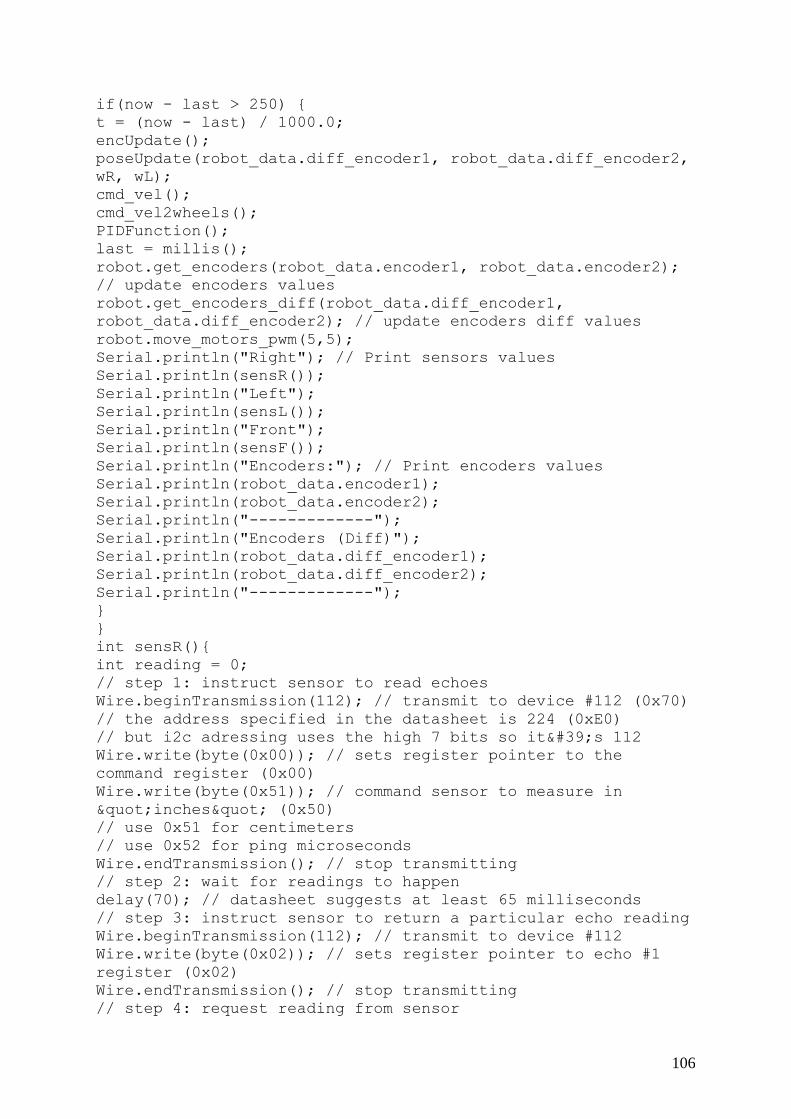
106
if(now - last > 250) {
t = (now - last) / 1000.0;
encUpdate();
poseUpdate(robot_data.diff_encoder1, robot_data.diff_encoder2,
wR, wL);
cmd_vel();
cmd_vel2wheels();
PIDFunction();
last = millis();
robot.get_encoders(robot_data.encoder1, robot_data.encoder2);
// update encoders values
robot.get_encoders_diff(robot_data.diff_encoder1,
robot_data.diff_encoder2); // update encoders diff values
robot.move_motors_pwm(5,5);
Serial.println("Right"); // Print sensors values
Serial.println(sensR());
Serial.println("Left");
Serial.println(sensL());
Serial.println("Front");
Serial.println(sensF());
Serial.println("Encoders:"); // Print encoders values
Serial.println(robot_data.encoder1);
Serial.println(robot_data.encoder2);
Serial.println("-------------");
Serial.println("Encoders (Diff)");
Serial.println(robot_data.diff_encoder1);
Serial.println(robot_data.diff_encoder2);
Serial.println("-------------");
}
}
int sensR(){
int reading = 0;
// step 1: instruct sensor to read echoes
Wire.beginTransmission(112); // transmit to device #112 (0x70)
// the address specified in the datasheet is 224 (0xE0)
// but i2c adressing uses the high 7 bits so it's 112
Wire.write(byte(0x00)); // sets register pointer to the
command register (0x00)
Wire.write(byte(0x51)); // command sensor to measure in
"inches" (0x50)
// use 0x51 for centimeters
// use 0x52 for ping microseconds
Wire.endTransmission(); // stop transmitting
// step 2: wait for readings to happen
delay(70); // datasheet suggests at least 65 milliseconds
// step 3: instruct sensor to return a particular echo reading
Wire.beginTransmission(112); // transmit to device #112
Wire.write(byte(0x02)); // sets register pointer to echo #1
register (0x02)
Wire.endTransmission(); // stop transmitting
// step 4: request reading from sensor
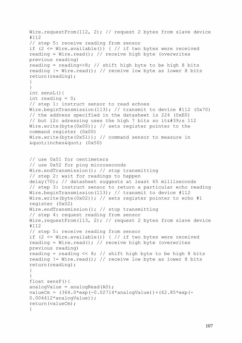
107
Wire.requestFrom(112, 2); // request 2 bytes from slave device
#112
// step 5: receive reading from sensor
if (2 <= Wire.available()) { // if two bytes were received
reading = Wire.read(); // receive high byte (overwrites
previous reading)
reading = reading<<8; // shift high byte to be high 8 bits
reading |= Wire.read(); // receive low byte as lower 8 bits
return(reading);
}
}
int sensL(){
int reading = 0;
// step 1: instruct sensor to read echoes
Wire.beginTransmission(113); // transmit to device #112 (0x70)
// the address specified in the datasheet is 224 (0xE0)
// but i2c adressing uses the high 7 bits so it's 112
Wire.write(byte(0x00)); // sets register pointer to the
command register (0x00)
Wire.write(byte(0x51)); // command sensor to measure in
"inches" (0x50)
// use 0x51 for centimeters
// use 0x52 for ping microseconds
Wire.endTransmission(); // stop transmitting
// step 2: wait for readings to happen
delay(70); // datasheet suggests at least 65 milliseconds
// step 3: instruct sensor to return a particular echo reading
Wire.beginTransmission(113); // transmit to device #112
Wire.write(byte(0x02)); // sets register pointer to echo #1
register (0x02)
Wire.endTransmission(); // stop transmitting
// step 4: request reading from sensor
Wire.requestFrom(113, 2); // request 2 bytes from slave device
#112
// step 5: receive reading from sensor
if (2 <= Wire.available()) { // if two bytes were received
reading = Wire.read(); // receive high byte (overwrites
previous reading)
reading = reading << 8; // shift high byte to be high 8 bits
reading != Wire.read(); // receive low byte as lower 8 bits
return(reading);
}
}
float sensF(){
analogValue = analogRead(A0);
valueCm = (364.0*exp(-0.02714*analogValue))+(62.85*exp(-
0.004412*analogValue));
return(valueCm);
}
108
void encUpdate() {
robot.get_encoders_diff(robot_data.diff_encoder1,
robot_data.diff_encoder1);
}
void poseUpdate(int NL, int NR, float &wR, float &wL) {
float DR, DL, D, vr, wr;
DR = (2.0 * PI * r / C * NR);
DL = (2.0 * PI * r / C * NL);
D = (DR + DL) / 2;
wr = ((DR - DL) / b) / t;
vr = D / t;
Pos.teta += (DR - DL) / b;
Pos.x += D * cos(Pos.teta);
Pos.y += D * sin(Pos.teta);
wR = (vr + b/2 * wr) / r;
wL = (vr - b/2 * wr) / r;
//Serial.print(“Real w right”);
//Serial.println(wR);
//Serial.print(”Real w left”);
//Serial.println(wL);
}
void cmd_vel() {
v = 1.0;
w = 0.0;
}
void cmd_vel2wheels() {
wLd = (v - b/2 * w) / r;
wRd = (v + b/2 * w) / r;
//Serial.print(“Desired w Left”);
//Serial.println(wLd);
//Serial.print(“Desired w Right”);
//Serial.println(wRd);
}
void PIDFunction() {
float PropErrorNow[2], PropError[2], DerivError[2],
IntgError[2], G[2];
PropErrorNow[0] = wRd - wR;
PropErrorNow[1] = wLd - wL;

109
DerivError[0] = PropErrorNow[0] - PropError[0];
DerivError[1] = PropErrorNow[1] - PropError[1];
IntgError[0] += PropErrorNow[0];
IntgError[1] += PropErrorNow[1];
// Updating proportional error
PropError[0] = PropErrorNow[0];
PropError[1] = PropErrorNow[1];
//If wheel tilts, decrease Kp
// If wheel is so slow, increase Ki
// If wheel is too fast, increase Kd
// Calculate PID output
G[0] = (0.8 * PropError[0]) + (2.5 * IntgError[0] * t) + (0.02
* DerivError[0] / t);
G[1] = (0.8 * PropError[1]) + (2.5 * IntgError[1] * t) + (0.02
* DerivError[1] / t);
robot.move_motors_pwm(G[0], G[1]); //0 is right and 1 is left,
motorboard (bottomboard) always at the back
}

110
Appendix B – Crack Detection, Python Code
import cv2
import numpy as np
import os
from PIL import Image
path = '/home/pi/images/'
#path = './images/'
cropped_path = '/home/pi/cropped/'
#cropped_path = './cropped/'
if not os.path.exists(cropped_path):
os.makedirs(cropped_path)
images = os.listdir(path)
prefix = 'cropped-'
def cv_size(img):
return tuple(img.shape[1::-1])
def detectCracks(fname, idx):
imagePath = cropped_path+prefix+fname
print("Running crack detection on " + imagePath)
image = cv2.imread(imagePath)
#image = cv2.bitwise_not(image) ##### We need to invert
the image here
size = cv_size(image)
max_size = max(size[0], size[1])
h = int(max_size / 50)
gray =
cv2.fastNlMeansDenoisingColored(image,None,h,21,7,21)
gray = cv2.cvtColor(gray, cv2.COLOR_BGR2GRAY)
gray = cv2.GaussianBlur(gray, (1, 1), 0)
median = np.median(image)
average = np.average(gray)
m = median
sigma = 0.25
threshold_min = int(max(0, sigma * m))
threshold_max = int(min(255, sigma * m))
gray = cv2.Canny(gray, threshold_min, threshold_max)
thresh = cv2.threshold(gray, threshold_min, threshold_max,
cv2.THRESH_BINARY)[1]
_, contours, _ = cv2.findContours(thresh.copy(),
cv2.RETR_EXTERNAL, cv2.CHAIN_APPROX_TC89_L1)
valid_contours_indices = []
for i in range(len(contours)):

111
if (i in valid_contours_indices):
continue
c = contours[i]
area = cv2.contourArea(c)
(x1, y1, w, h) = cv2.boundingRect(c)
neighbors = []
for c2 in contours:
(x2, y2, _, _) = cv2.boundingRect(c2)
d = np.sqrt((x2-x1)**2 + (y2-y1)**2) # euclidian
distance
if (d < .5*max_size):
neighbors.append(c2)
if ((len(neighbors) > .2*len(contours)) and (w+h>5)
and (area <= ((size[0]*size[1])-100))):
valid_contours_indices.append(i)
print("Found {} contour(s) and {}
valid".format(len(contours), len(valid_contours_indices)))
for i in valid_contours_indices:
cv2.drawContours(image, contours, i, (0, 0, 255), 3)
cv2.namedWindow('Image ' + idx, cv2.WINDOW_NORMAL)
cv2.resizeWindow('Image ' + idx, 500,500)
cv2.imshow('Image ' + idx, image)
if __name__ == "__main__":
for fname in images:
if fname.endswith('.jpg'):
print("cropping image : ", fname)
img = Image.open(path+fname)
w, h = img.size
offset = 185
img = img.crop((offset, offset, w-offset,w-
offset))
img.save(cropped_path+prefix+fname)
detectCracks(fname, fname)
cv2.waitKey()
cv2.destroyAllWindows()

112
Appendix C – Image Capture, Python Code
import time
import picamera
count = 0
camera = picamera.PiCamera()
while True:
camera.capture('./images/crack' + str(count) + '.jpg')
time.sleep(0.23)
count += 1
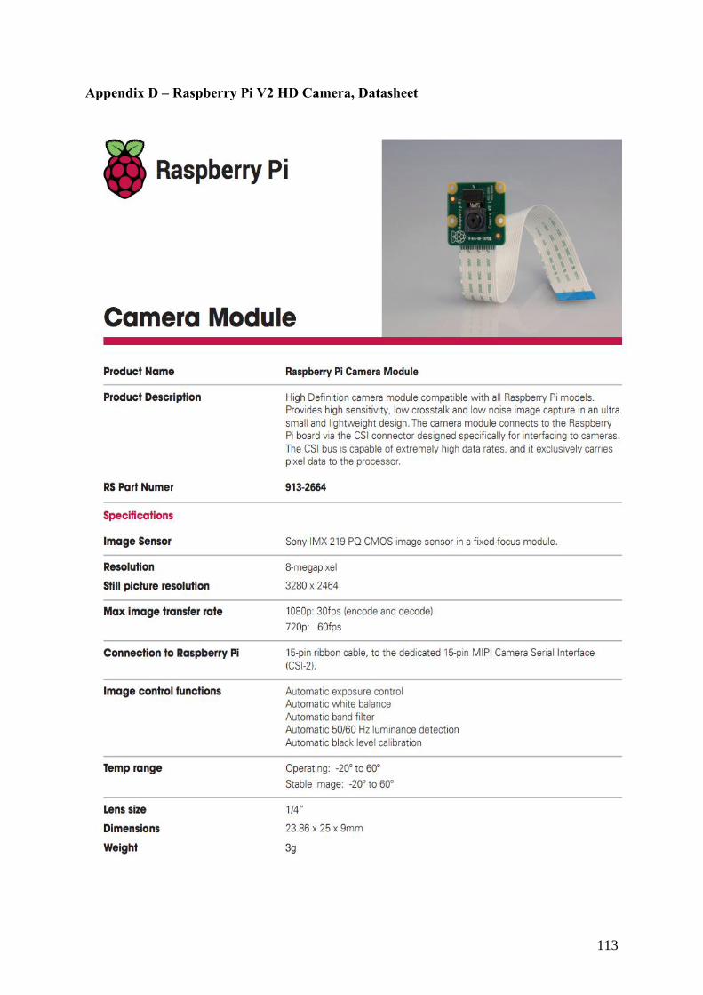
113
Appendix D – Raspberry Pi V2 HD Camera, Datasheet
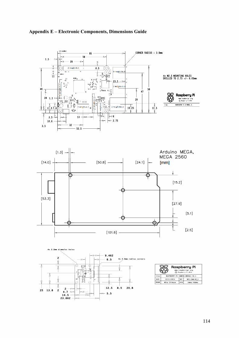
114
Appendix E – Electronic Components, Dimensions Guide
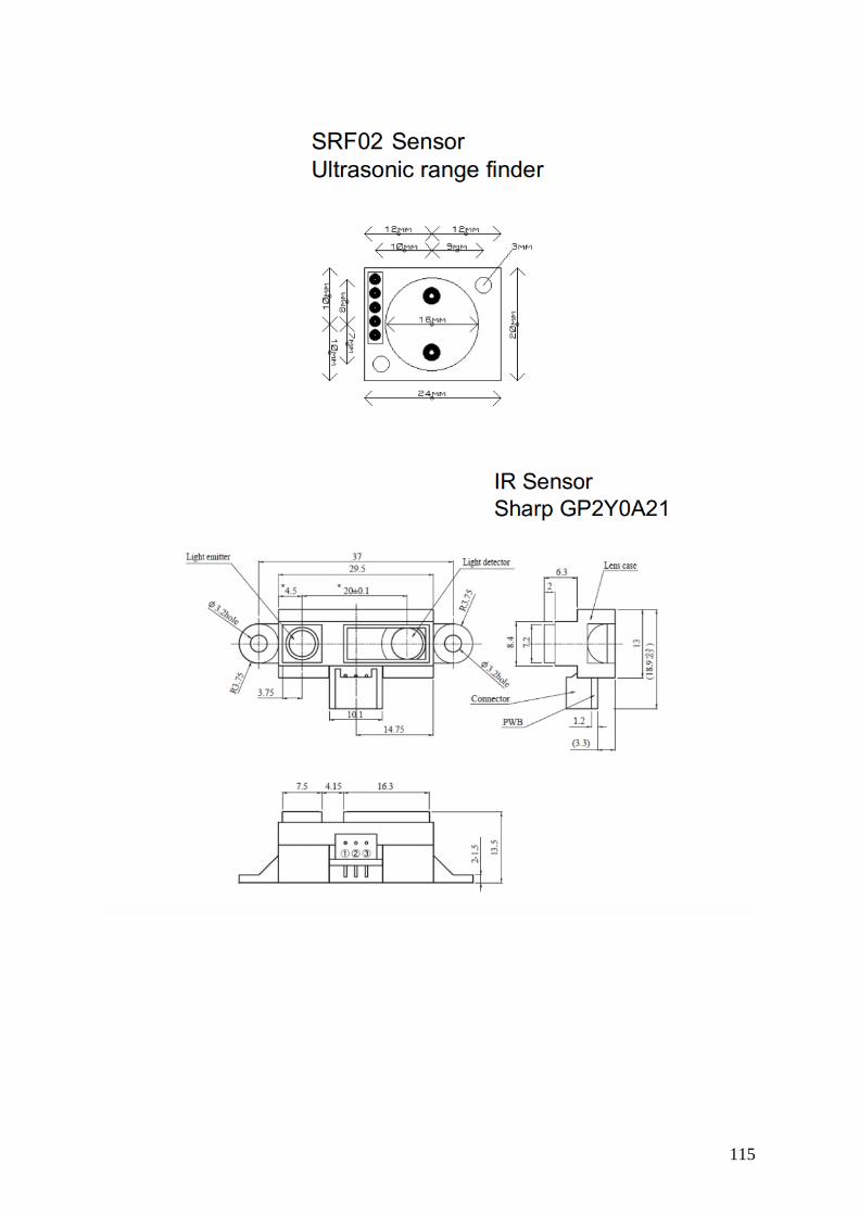
115