The Convergence of Market Designs for Adequate Generating Capacity with Special Attention to the CAISO’s Resource Adequacy Problem

A White Paper for the Electricity Oversight Board

Peter Cramton and Steven Stoft

25 April 2006

Contents 1. Preamble ..............................................................................................................2 2. Summary..............................................................................................................3 3. What Is the Resource Adequacy Problem?......................................................8 4. A Comparison of Ten Approaches..................................................................12 5. Summary of Proposed Solution ......................................................................15

The Standard Example 15 Basic Forward-Capacity-Market Design 16 Benefits of the FCM Design 17

6. What the Market Can’t Do.................................................................................20 7. The “Energy-Only” Approach..........................................................................26

The Centrally-Planned Energy-Only Demand Curve 26 Central Planning of Quantity Leaves Room for the Market 28

8. Replacing the Missing Money..........................................................................30 The ICAP Approach 31 Hogan’s Energy-Only Approach 32 Other Energy-Only Approaches Ignore the Missing Money 33

9. Controlling Reliability: Spot Prices or Capacity Targets? ............................39 Stable Control of Capacity Using Capacity Targets 39 Erratic Control with Spot Energy Prices 40

10. Spot Energy Prices Make the Best Performance Incentives ........................44 Why Value-Reflective Prices are Irreplaceable 44 Hedging Price Spikes 45

11. Assembling a Basic Design .............................................................................48 Step 1: Design Full-Strength Spot Prices 48 Step 2: Hedge All Load with Call Options 49 Step 3: Purchase an Adequate Level of Hedged Capacity 51

12. Additions to the Basic Design .........................................................................55 13. The Final Step to Convergence .......................................................................59 14. Conclusion.........................................................................................................63 15. Appendix 1: Terms and Symbols ...................................................................64 16. Appendix 2: Frequently Asked Questions.....................................................65 17. References.........................................................................................................70

1

The Convergence of Market Designs for Adequate Generating Capacity With Special attention to the CAISO’s Resource Adequacy Problem

A White Paper for the Electricity Oversight Board 1

Peter Cramton and Steven Stoft 2

Abstract

This paper compares market designs intended to solve the resource adequacy (RA) problem, and finds that, in spite of rivalrous claims, the most advanced designs have nearly converged. The original dichotomy between approaches based on long-term energy contracts and those based on short-term capacity markets spawned two design tracks. Long-term energy contracts led to call-option obligations which provide market-power control and the ability to strengthen performance incentives, but this approach fails to replace the missing money at the root of the adequacy problem. Hogan’s (2005) energy-only market fills this gap. On the other track, the short-term capacity markets (ICAP) spawned long-term capacity market designs. In 2004, ISO New England proposed a short-term market with hedged performance incentives essentially based on high spot prices. In 2005, we developed for New England a forward capacity market, with load obligated to purchase a target level of capacity covered by an energy call option. The two tracks have now converged on two conclusions: (1) High real-time energy prices should provide performance incentives. (2) High energy prices should be hedged with call options. We argue that two more conclusions are needed: (3) Capacity targets rather than high and volatile spot prices should guide investment, and (4) Long-term physically based options should be purchased in a forward market for capacity. The result will be that adequacy is maintained, performance incentives are restored, market power and risks are reduced from present levels, and prices are hedged down to a level below the present price cap.

1 We are grateful for funding from California's Electricity Oversight Board and the National Science Foundation. 2 We thank the ISO-NE team for unflagging support in the form of new ideas, reality checks and patience with many revisions to the market designs. We also thank Erik Saltmarsh of the EOB for help with the California context and for providing this opportunity to freely discuss such a controversial and timely area of market design. We are grateful for helpful comments from EOB staff. The views in this paper are solely the views of the authors and do not represent the views of EOB or ISO-NE.

2

1. Preamble California may need new capacity even sooner than it can be built, but implementing a useful resource adequacy (RA) program takes time. In the mean time, it is better to use a clean, well-tested, stop-gap measure, such as RFPs for new generation, than to implement a half-baked temporary RA program. The erroneous structures and commitments implemented by such a program will be painful to dispose off, as is still being demonstrated by California’s last round of long-term contracts.

There is also an economic reason to avoid a temporary RA program. It will not work. RA programs, whether short-term ICAP markets or long-term energy contract markets, work, if they do, by signaling investors that they can expect stable and reasonable cost-recovery for many years to come. No temporary program can achieve this. It is just not in the nature of “temporary.”

Even long-term energy-contract proposals cover at most the first three years of a new twenty-plus year investment, and many do not cover even the first minute, because they terminate before any new project could go on line. Even if a temporary RA program required five-year contracts starting three years from the requirement date, such contracts would be forced to include a hefty risk premium to be effective. Why? Because the new investor would still face a completely unknown cost-recovery regime at the end of those five years. At least fifteen out of 20 years (and most likely 20 out of 20 years) of necessary cost recovery will be up for grabs when a temporary program’s contract is signed.

RA programs do not accomplish much with their monthly payments or even with a year or two of contract coverage starting after the plant is built. They achieve their goals through expectations. When Intel builds a new chip-fabricating plant, it does not do so on the basis of contracts for chip sales from that plant. Those chips have not even been designed. It builds fabricating capacity completely on the basis of positive expectations. RA programs that work, must replace the enormous regulatory risk of the present with expectations of stable cost recovery for twenty years. This is no easy task, and an RA policy stamped “TEMPORARY,” cannot succeed. It may pay out large sums of money, which will be gladly accepted by existing generation, but it will not induce new investment at anything close to a reasonable price.3

Since a temporary program is needed, how can this dilemma be avoided? Very simply. Sign truly long-term contracts with investors who build new generation. This will give these particular suppliers the strong expectations of long-term stable cost recovery that they require before they can charge the consumers of California a low risk premium. With the assurance of a truly long-term contract, competition among proposals can hold the price down to a reasonable level. Using a temporary RA program is an expensive new idea that should be retired as quickly as possible. Using RFPs for this purpose is not a clever new idea, but it works.

3 In fact, for an existing supplier, a failing RA program would be ideal, since existing generation would be paid, but no new competitors would enter the market.

3

2. Summary The core recommendation of this paper is to use the best design features from the various existing RA approaches; all have something to offer. Use the capacity targets of the ICAP design track, the High Spot Prices and call options of the energy-only track, and a centralized forward market which is found in both design tracks. As Singh first noted in 2000, elements from the energy-only and ICAP tracks are not fundamentally antagonistic but can be used to complement each other. This is demonstrated by the forward capacity market (FCM) design developed for ISO-NE and described below.

The resource adequacy problem. The goal of resource adequacy is to minimize consumer cost including the cost of blackouts, but the central problem of resource adequacy is to restore the missing money that prevents adequate investment in generating capacity. More precisely, the problem is that current market-design parameters, such as offer caps, have been set to control market power, and consequently have been set too low for adequacy. Current energy markets underpay investors whenever investment brings capacity close to the adequate level. The result is that investment stops well before reaching the adequate level.

The amount of money missing when capacity is adequate has been estimated in ISO-NE at over $2 billion per year. More importantly, at the adequate capacity level, peakers can expect to cover perhaps as little as one quarter of their fixed costs. The CAISO’s lower offer cap of $250 leaves less room for fixed-cost recovery.

The root cause of the RA problem is a pair of demand side flaws which make it impossible for the market to assess, even approximately, the value placed on reliability by consumers. Without information on the value of reliability, the market cannot determine the adequate level of capacity, since that is defined by the value of reliability.

A comparison of ten approaches. This section summarizes four theoretical energy-only approaches, the standard ICAP approach used in Eastern markets, a theoretical long-term ICAP approach and four convergent approaches, two of which are theoretical. The other two are the LICAP approach largely accepted for ISO-NE by the FERC’s administrative law judge, and a forward market design presented here as a theoretical design, but which is mimicked fairly closely by the current stakeholder compromise in New England.

These proposals are judged according to six fundamental design choices. (1) Is adequate capacity explicitly targeted? (2) Is the missing money restored? (3) Do the forward contracts cover new capacity? (4) Are the required contracts purely financial? (5) Are performance signals market-based? (6) To what extent is load hedged?

Energy-only markets fail to target capacity, and with one exception, fail to restore the missing money. Standard ICAP designs fail to provide market-based incentives and hedge load. (Failure to hedge load, also indicates a failure to hedge capacity and reduce spot market power.) Convergent designs do better, and the forward capacity market presented here is designed to show that all six choices can be made correctly—there is no need for a tradeoff.

4

Proposed solution. To solve the RA problem, the missing money must be restored without reintroducing the market power problems currently controlled by price suppression. Moreover, inadequate investment is not the only problem caused by energy-price suppression; it is only the most obvious. Crucial performance and quality incentives are also missing. All of these problems can be solved with a three step design process. Step 1: Design full-strength spot prices Step 2: Hedge all load with call options Step 3: Purchase an adequate level of hedged capacity

The full-strength, High Spot Prices solve the problems caused by suppressing spot prices, but would reintroduce market power and risk problems were they not hedged. Call options that cover all load eliminate these side effects while perfectly preserving the performance and quality incentives of the high prices. All that remains, to restore the missing money and induce an adequate level of capacity, is to pay enough for the capacity-backed hedges.

Either a short-term or a forward capacity market (FCM) can be used to buy the capacity at the market price. An FCM is recommended. It buys capacity three years in advance, and gives new capacity multi-year contracts. Existing capacity receives annual contracts at a similar price. The combination provides a low-risk environment for investors, which greatly reduces the risk premiums passed on to load.

What the market can’t do. The market, without administrative guidance, cannot determine what level of installed capacity is needed to provide adequate reliability. This is a consequence of two Demand-Side Flaws caused by infrastructure problems that will not be remedied for perhaps another decade or more. The administrator has only two choices: set key market parameters without regard for their investment consequences, or adopt a conscious resource adequacy program.

This point is important, because one of the most widely accepted reasons for choosing one RA approach over another is the notion that one provides more (or complete) market guidance with respect to how much capacity is adequate. Unfortunately, current markets provide no guidance whatsoever, except by passing through guidance (or confusion) from administrators. For example, MISO states “The principal reason for considering an energy-only market approach … is the expectation that it would allow market incentives, rather than centralized administrative direction, to drive investment decisions.” This reason is not correct.

The energy-only approach. Hogan’s (2005) proposal of an energy-only approach is the inspiration for the MISO’s hope of avoiding centralized administrative direction. Yet the transfer of missing money used by that proposal to solve the adequacy problem is controlled by an administratively determined energy+reserve demand curve. The parameters set by administrators fully control the flow of all scarcity revenues above the variable cost of a new peaker. That could amount to $4 billion annually in a 50 GW market. Hence, the energy-only approach, if designed to restore missing money, is no-more free of central planning than an ICAP approach.

5

This does not mean markets cannot play a crucial role. In fact they should be given full control of all the more difficult investment issues. They are needed to assure the low cost, high quality, and performance of the capacity purchased, to select who should build and where plants should be built, to determine the proportion of base-load plants, and much more.

Replacing the missing money. ICAP markets are designed specifically to replace the missing money, caused by spot-price suppression, and thereby restore adequate capacity. ICAP pays all existing capacity enough to let new entry break even when capacity is adequate. Hogan’s energy-only-market approach also tackles the missing money problem directly, and solves it by raising the offer cap to something like $10,000/MWh. The cap depends on the value of lost load, which is generally estimated to be somewhere between $2,000/MWh and $250,000/MWh.

Past energy-only approaches have focused on obligating load to buy more call options or long-term energy contracts, and have ignored the missing money problem. The approach assumes that a lack of hedging, and not missing money, is the cause of the RA problem. Such energy-only approaches provide no mechanism for replacing the missing money. Oren (2005), advocating call-option obligations, is helpful in explaining this omission.

Spot prices vs. capacity targets. There are two approaches to controlling the resource

level (installed capacity). The most direct uses a capacity target. For example standard ICAP markets use an explicit capacity demand function, which pays investors more than enough when the market is short of capacity, and less than enough when it has extra capacity. The outcome of a capacity-target approach is relatively predictable.

By contrast, a spot price approach uses an implicit capacity-demand function which is nearly impossible to estimate theoretically and can require many years of data to estimate empirically. Eighteen years of data from the New England market fails to show any relationship between capacity and spot energy prices, and in particular fails to show spot energy prices increasing sharply as capacity falls below a target level.

Spot prices as performance incentives. Economists advocate markets because competitive prices provide efficient incentives to both sides of the market. The suppression of spot prices, which led to the adequacy problem, dramatically reduced hundreds of different performance and investment signals, not just the signal that controls the quantity of investment. The obvious solution is to restore the spot prices, but this is impractical unless load is fully hedged with call options, which prevent the return of market power and risk problems.

Call options do not solve the adequacy problem, or performance, or quality problem. They simply allow the use of the market solution to the performance problem while protecting consumers from market power and risk.

A complete Basic Design. The design follows the three steps listed above. It builds on an energy market, with “normal” and “scarcity” revenues, NR and SR, defined as coming from prices below and above the strike price of a call option.

6

Step 1. The scarcity rents of performing capacity suppliers are increased to M × SR. Step 2. Load is completely hedged, meaning all suppliers must pay load M × SRShare Step 3. A capacity market determines the price, PIC, of hedged capacity.

The scarcity-revenue multiplier, M, restores, in effect, full strength spot pricing. Each supplier’s hedge (call option) is responsible for its “Share” of load plus operating reserves, which is proportional to its share of total capacity, 10% if it sold 5 out of a total of 50 GW. On average, suppliers break even on scarcity revenue, and load pays no scarcity revenue directly. Instead load pays the auction price for the hedge against scarcity revenues, PIC. The formula for the supplier’s revenue in both markets is:

[NR + SR] + [PIC – SRShare + (M – 1) ( SR – SRShare ) ]

Energy Market + Capacity Market

As a direct consequence of these formulas, any supplier that covers its Share of load will have SR = SRShare and will receive exactly NR + PIC. The capacity price, PIC, can be set by either a short-term or forward capacity market, but a forward market is recommended. A supplier that does not supply its share will do worse by M × ( SR – SRShare ). Full-strength performance incentives are such that in expectation, for a resource that never performs, this deduction exactly offsets the capacity price PIC.

Additions to the Basic Design. The Basic Design simply illustrates key principles, and is missing many important practical features. These include (1) market power controls in the FCM auction, (2) the descending clock auction, (3) the call options details (4) capacity export rules, (5) lumpy supply bid rules, and (6) a definition of capacity.

The final step to convergence. The most advanced designs on the energy-only and ICAP design tracks have converged on two fundamental design principles: (1) use restored High Spot Prices for performance incentives, and (2) hedge these prices with call options. But a fundamental distinction remains between the two tracks.

The ICAP approach requires all supply that receives High Spot Prices to hedge load against those prices. The energy-only approach does not. It implements a $10,000 offer cap for all load and supply regardless of the hedge. This causes two problems which the ICAP approach avoids. (1) As intended, the High Spot Prices dominate the mandatory load hedge in the control of the adequate resource level, so this control is erratic. (2) As Hogan and Harvey (2000) argued by giving supplier’s market power (now with a $10,000 price cap instead of the $250 price cap in place at the time), load will be forced to buy back this market power when it buys the long-term mandatory hedges of the energy-only approach.

Conclusion. The promise of restructuring was not better dispatch, but better investment and operation. To date this has not been realized. In fact, with boom-bust investment cycles and regulatory risk causing exorbitant risk premiums, consumers may be worse off than under the stable environment of regulation. Efficient spot prices held out the promise of better investment choices and better operation, but those prices have

7

now been cut to a fraction of their proper level. This has caused the RA problem and dramatically diminished signals for investment quality and supplier performance.

By coherently combining the best features of the two RA design tracks, all three of these problems can be solved without reintroducing the market power, risk and instability problems of the previous High-Spot-Price regime. To accomplish this, first design full-strength spot prices. Second, restore these High Spot Prices only to suppliers which completely hedge load with a call option. Third, purchase an adequate level of hedged capacity. Let the market determine how high a price must be paid to induce this adequate resource level.

The High Spot Prices will solve the quality and performance problems. The hedge will prevent the return of market power and risk problems and will even reduce the present level of these concerns. Finally, the capacity market, preferably using a forward auction and multi-year contracts for new supply, will provide a stable level of adequate capacity and stable energy/capacity prices. This will provide consumers with reliability at the lowest cost.

8

3. What Is the Resource Adequacy Problem? In a review of older capacity-market initiatives, Bushnell (2005) analyzes six goals of resource adequacy mechanisms, but concludes that “Missing from this list is the overarching goal of providing reliable electricity service at the lowest possible cost.” This is a fair criticism of older energy-only and capacity-market designs and even of the recent proposals of Hogan (2005) and Oren (2005), which do not address the problem from this perspective. However, the CPUC’s (2005) ICAP proposal states this overarching goal explicitly,4 as does PJM’s proposal.5 ISO New England’s recent proposal also makes use of it frequently. “Taken together, these features of the proposed design will minimize long-run consumer costs, including all costs of generation and the cost of possible blackouts from inadequate generation capacity.” (Stoft 2004, p. 9). The frequent application of this principle becomes apparent in such phrases as “how to minimize those costs by reducing capacity volatility and investor risk” (Stoft 2005, p. 0).

But neither the six goals identified by Bushnell, nor the overarching goal of long-run cost minimization, constitute the RA problem. The central problem, labeled “missing money,” is that, when generating capacity is adequate, electricity prices are too low to pay for adequate capacity. This problem is recognized by all capacity-market approaches and by Hogan’s energy-only approach, but not by other energy-only approaches. The consequence of this problem is a long-run average shortage of capacity and too little reliability.

Considered narrowly, the problem is caused by the low settings of several key market-design parameters, such as the offer cap. Initially, most markets were un-capped and price spikes over $5000/MWh were observed for several years running in Eastern and Midwest markets. During that period, markets with adequate capacity seemed to be paying incumbent generation generously enough. In fact, a market with a $10,000 cap triggered by any shortage of operating reserves will quite likely pay enough or more. Too much reliability is as possible as too little. This raises the broader question of why the parameters are set too low and not too high or just right. The problem behind the problem is two-fold. Economics provides no easy answer to “what is the correct design,” and social pressures have, on balance, favored low prices.

With no clarity regarding design parameters and prices regularly reaching more than 100 times their normal level, sometimes under questionable circumstances, pressures from load overpowered those from suppliers and market designs were modified to produce lower prices. Price caps were set at between $250 and $1000/MWh, and ISOs learned many ways of mitigating prices. This was not the wrong first step, though some excesses have been committed. Lower price caps and some price mitigations solve very real problems caused by market power and risk. But, these changes are partial and unbalanced, with the result that investors are missing money. 4 “The primary purposes of the Commission’s RA requirements are: … (2) to ensure that this investment is provided in a way that minimizes total consumer cost of delivered power over the long run.” (CPUC, 2005, p. 1) 5 “Capacity markets should be designed to dampen boom-bust cycles, improve the stability and predictability of system adequacy, and minimize costs to consumers.” (Hobbs, 2005.)

9

A full understanding of the RA problem requires that its source be pushed back one level further. An explanation is needed for why regulators are in the business of setting market parameters that control investment. This complex and contentious issue is discussed at length in Section 6, “What the Market Can’t Do.” As indicated in Figure 1 above, current electricity markets contain Two Demand-Side Flaws which prevent the market from solving the reliability problem and hence the investment problem which is the other side of the same coin. Figure 1 provides an overview of the complete cause of the resource adequacy problem. Two demand-side flaws, which cannot be eliminated for some time, cause regulators to intervene. Market power concerns cause this intervention to be biased towards low scarcity rents which are obtained by setting parameters such as the price cap (PCap) and operating reserve parameters (OpRes) too low for investment purposes. This reduces scarcity revenue, resulting in missing money, (as determined at that adequate level of capacity), which in turn, discourages investment before the adequate level of capacity is reached. This leaves the market in a precarious position.

Other Market Problems ( addressed by energy-only )

Two Demand-Side Flaws Real-time: 1. meters, 2. disconnect

Market Frictions

Regulators must set investment parameters ( PCap, OpRes )

Parameters set too low for reliable investment

Missing Money ( when investment is adequate )

Too Little Investment

Lack of Reliability Periodic Crises

Market Intervention

High cost of investing

Market Power Risk

Wealth transfers Inefficiency

Poor Incentives for Performance

Investment Quality

Figure 1. Causes of Market Problems

Resource Adequacy Problem ( addressed by ICAP )

10

Either regulators will intervene, or capacity will fall towards a point at which investment would resume. With a price cap of $250, this might require the cap to be reached for roughly 400 hours per year, but with the market this tight, a crisis is likely.

The right side of Figure 1 shows two other market problems which have been mistaken for the RA problem, particularly in the West. The market power problem can be more efficiently solved by long-term contracts than by market-power mitigation, as has been argued since before the California crisis by Wolak (2004). Once, the RA problem came to prominence, his long-term contract proposal was simply labeled as the solution to that problem. As will be discussed in Section 8, “Replacing the Missing Money,” Wolak’s long-term contract proposals contain no mechanism for shifting the required amount of revenue in the face of low price caps.

The call-option approaches of Oren and of Chao and Wilson are also diagramed on the right of Figure 1. These were developed to solve another real problem, investment risk. Unlike the long-term contract approach, these were directed at the RA problem from the start. Again, they are helpful and even feed into the solution of the RA problem in a helpful manner. But, they do not address the central dilemma of that problem, and cannot come close to solving it, unless they are coupled with a capacity market type of mechanism.

Fortunately, there is no conflict whatsoever between these three approaches to solving three different problems. The best solution to the RA problem utilizes long-term call options in a long-term capacity market framework. Moreover, this combined approach also solves the performance incentive problems created as side-effects of the price cap and other parameters being set too low. This paper shows how this combination of approaches is best realized.

The missing money is the step in the RA causal chain most easily quantified, and doing so serves to put the problem in perspective. How much is missing? The best estimate from ISO-NE is that, with adequate capacity, it will have 20 to 25 shortage hours per year. During these hours the price might reach $1000, though that does not happen automatically until the fifth such hour in a row. At most, this market should provide about 25 × (1000 – 100), or $22,500/MW-year in peaker fixed-cost recovery. ISO-NE estimates the fixed cost of a new peaker, the cheapest capacity, at roughly $95,000/MW-year.6 With a 30,000 MW market, they are missing over $2 billion per year. From the investor’s point of view, when capacity is adequate, peakers can expect to cover only one quarter of their fixed costs. No one with such expectations will invest.

The CAISO market appears to be similar. Its price caps are four times lower and over five times closer to the variable cost of a peaker. So they need five times as many shortage hours as New England to reach the same level of fixed-cost recovery. This seems unlikely with adequate capacity, so missing money should be expected. Estimates for NYISO and PJM have yielded similar result.

6 A peaker is used because every system needs peakers and must pay for them on average, and because they are easier to calculate required scarcity rents for. For a more complete analysis, see FAQ 1 in the appendix.

11

Those confronted with this problem sometimes reply, “but remember, there may be price spikes again like in 2000—2001, and so the average may not be as low as it looks.” But the missing money estimates, noted above, are for years with adequate capacity. Economics tells us the market will take care of itself and there should be no missing money at all. But that assumes installed capacity will be allowed to fall as far as it needs to provide suppliers with high prices—regardless of the impact on reliability. The missing-money problem is not that the market pays too little, but that it pays too little when we have the required level of reliability.

Another response to the missing money problem is, “Just get out of the way and let the market take care of it. The problem is simply the result of meddling.” Many have taken this seriously, but without success. No coherent workable pure-market solution has ever been proposed. As already noted, this point is addressed by the two Demand-Side Flaws and discussed in Section 6.

What is required is a mainly-market solution. One in which the market administrator selects the adequate level of capacity and designs the market parameters to induce the market to provide that level as cheaply as possible. This still leaves the most important role to the market, but the administrator must solve the problem of what level of installed capacity is adequate, because the markets do not yet have the necessary infrastructure. This paper explains how to design such a market and adjust its parameters to solve the adequacy problem while maximizing beneficial and minimizing detrimental side effects.

In summary, the resource adequacy problem is the problem of missing money. This problem can be traced to price suppression which in turn can be traced back further. Inevitably, price suppression has caused other problems as well, most notably, degraded performance and investment-quality incentives.

12

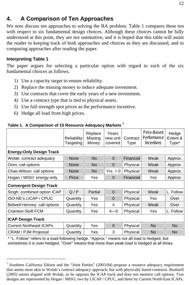
4. A Comparison of Ten Approaches We now discuss ten approaches to solving the RA problem. Table 1 compares these ten with respect to six fundamental design choices. Although these choices cannot be fully understood at this point, they are not unintuitive, and it is hoped that this table will assist the reader in keeping track of both approaches and choices as they are discussed, and in comparing approaches after reading the paper.

Interpreting Table 1 The paper argues for selecting a particular option with regard to each of the six fundamental choices as follows.

1) Use a capacity target to ensure reliability. 2) Replace the missing money to induce adequate investment. 3) Use contracts that cover the early years of a new investment. 4) Use a contract type that is tied to physical assets. 5) Use full-strength spot prices as the performance incentive. 6) Hedge all load from high prices.

Table 1. A Comparison of 15 Resource Adequacy Markets 7

Reliability Targeting

Replace Missing Money

Years new unit covered

Contract Type

Price-Based Performance

Incentives

Hedge Extent &

Type*

Energy-Only Design Track Wolak: contract adequacy None No 0 Financial Weak Approx. Oren: call options None No 0 Physical Weak Approx. Chao-Wilson: call options None No Yrs. > 0 Physical Weak Approx. Hogan / MISO: energy-only Price Yes 0 Financial Yes Approx.

Convergent Design Track Singh: combined option ICAP Q / P Partial 0 Physical Weak L. FollowISO-NE’s LICAP / CPUC Quantity Yes 0 Physical Yes Over Bidwell-Henney: call options Quantity Yes 4 Physical Weak Over Cramton-Stoft FCM Quantity Yes 4—5 Physical Yes L. Follow

ICAP Design Track Current Northeast ICAPs Quantity Yes 0 Physical No No CRAM / PJM Proposal Quantity Yes 3 Physical No No * “L. Follow” refers to a load-following hedge. “Approx.” means not all load is hedged, but sometimes it is over-hedged. “Over” means that more than peak load is hedged at all times.

7 Southern California Edison and the “Joint Parties” (2005/04) propose a resource adequacy requirement that seems most akin to Wolak’s contract adequacy approach, but with physically based contracts. Bushnell (2005) seems aligned with Wolak, as he opposes the ICAP track and does not mention call options. Two designs are represented by Hogan / MISO, two by LICAP / CPUC, and three by Current North-East ICAPs.

13

By and large, the energy-only approaches do well with respect to incentives and hedging, while the ICAP approaches do well with respect to solving the central RA problem. One surprise is that the call-option / long-term contract approaches do quite poorly with respect to requiring genuinely long-term contracts. Mostly they suggest contracts that expire before a plant can be built, but one may assume they would not object to longer terms.

A second surprise is the strength of showings in the Convergent Design Track. Moreover, Hogan’s new design (2005) comes close to crossing the line by being the first energy-only approach to face up to and solve the missing-money problem. Unfortunately it does not yet take a realistic approach to stabilizing investment, so it will perform poorly. Nonetheless it provides an important impetus to the move towards convergence.

Oren (2005) moves towards a convergent design from a different direction. He recommends a “centralized procurement of backstop call options by the system operator.” The CRAM approach, seen in the bottom row, is a forward ICAP market quite similar to the one proposed in this paper (Cramton-Stoft FCM).

The convergent design track was actually pioneered by Singh (2000) in his paper proposing to combine elements of ICAP and energy only markets by purchasing call options in an ICAP market. In summary, the energy-only approach has been strong on hedging and the use of spot prices to provide performance incentives, while the ICAP approaches have focused on replacing the missing money and targeting an adequate quantity. The Convergent design track embraces all of these benefits.

Some Evaluation Details Targeting. This factor determines the design track. ICAP designs target quantity, and

energy-only designs do not. As is explained in Section 9, targeting a capacity quantity, especially with a long-term ICAP auction, is a much more reliable way to assure resource adequacy than is administratively setting an energy-demand curve.

Money. RA approaches that do not replace the missing money, do not work. The first three energy-only approaches claim to be RA or generation adequacy mechanisms, but focus instead on the benefits of risk management and market power suppression.

Years. Although energy only approaches specify long-term contracts, this typically means less than three years. For example Wolak (2004) specified 75% coverage one year in advance with increasing coverage for shorter time periods.

Type. Significantly, the two energy-only approaches with the most sophisticated financial analysis, both specify physically based options as the appropriate method of inducing investment. All of the ICAP markets use physically-based contracts.

Incentives. Energy-only designs retain the energy price as the sole driver of investment. Were they to solve the investment problem, their performance incentives would automatically become full strength. This is not true of Bidwell and Henney’s ICAP-Option approach, which is why it is downgraded on performance incentives, even

14

though they are sensitive to this issue and agree that spot prices provide the best incentives.

Hedging. Even before the California crisis, Wolak was calling for long-term energy contracts because they suppress market power. This remains a key benefit of energy-only approaches. Hedges also reduce investor risk and the risk premiums they cause consumers to pay on all installed capacity, new and old. This sizable benefit is missed by traditional ICAP markets, but captured by the new designs. Although Oren and Chao/Wilson suggest load following, only Singh and Cramton/Stoft suggest implementing options that inherently follow the load.

In summary, ICAP approaches use a capacity target to send a clear adequacy signal and they solve the missing-money problem. Hence they solve the basic RA problem. Energy-only approaches provide improvements in risk, spot-market power, and performance incentives that are entirely overlooked by traditional ICAP approaches. Convergent designs combine the strengths of both approaches without sacrificing any benefits. Hogan’s new energy-only approach takes a major step towards a convergent design, and Oren’s call-option obligations provide further guidance towards a convergent design. ICAP designs have recently begun adopting energy-only features, and the FCM design presented here completes the convergence.

15

5. Summary of Proposed Solution This paper presents a forward capacity market (FCM) approach to assuring resource adequacy which was developed, at the request of load, for use by ISO-NE in its post-LICAP negotiations.8 Along the way it diagnoses the root cause of the adequacy problem, the limitations and potentials of a market approach, and demonstrates the importance of side-effects. Before embarking on this journey, it may be helpful to glimpse the destination. To that end, we begin by sketching, with many details suppressed, the FCM approach.

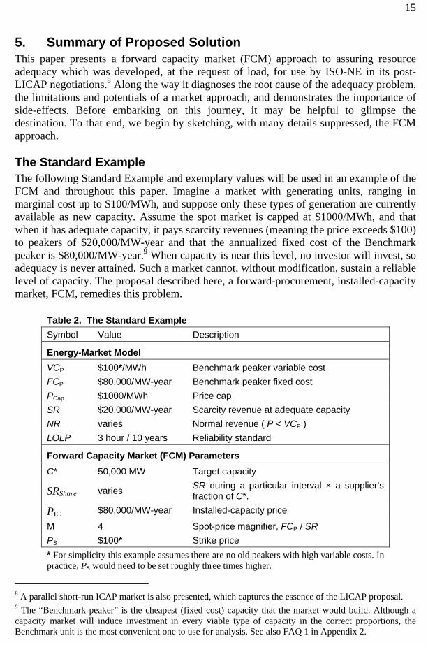
The Standard Example The following Standard Example and exemplary values will be used in an example of the FCM and throughout this paper. Imagine a market with generating units, ranging in marginal cost up to $100/MWh, and suppose only these types of generation are currently available as new capacity. Assume the spot market is capped at $1000/MWh, and that when it has adequate capacity, it pays scarcity revenues (meaning the price exceeds $100) to peakers of $20,000/MW-year and that the annualized fixed cost of the Benchmark peaker is $80,000/MW-year.9 When capacity is near this level, no investor will invest, so adequacy is never attained. Such a market cannot, without modification, sustain a reliable level of capacity. The proposal described here, a forward-procurement, installed-capacity market, FCM, remedies this problem.

8 A parallel short-run ICAP market is also presented, which captures the essence of the LICAP proposal. 9 The “Benchmark peaker” is the cheapest (fixed cost) capacity that the market would build. Although a capacity market will induce investment in every viable type of capacity in the correct proportions, the Benchmark unit is the most convenient one to use for analysis. See also FAQ 1 in Appendix 2.

Table 2. The Standard Example Symbol Value Description

Energy-Market Model VCP $100*/MWh Benchmark peaker variable cost FCP $80,000/MW-year Benchmark peaker fixed cost PCap $1000/MWh Price cap SR $20,000/MW-year Scarcity revenue at adequate capacity NR varies Normal revenue ( P < VCP ) LOLP 3 hour / 10 years Reliability standard

Forward Capacity Market (FCM) Parameters C* 50,000 MW Target capacity

SRShare varies SR during a particular interval × a supplier’s fraction of C*.

PIC $80,000/MW-year Installed-capacity price

M 4 Spot-price magnifier, FCP / SR PS $100* Strike price * For simplicity this example assumes there are no old peakers with high variable costs. In practice, PS would need to be set roughly three times higher.

16

Basic Forward-Capacity-Market Design The FCM design specifies that each year, at the end of March, an auction is held, which buys enough capacity, existing and new, to provide adequate capacity C* for the year starting three years from that date. Existing capacity will be purchased for one year and new capacity will be given four-year contracts.10

Both new and existing units will be paid an auction-clearing price, PIC, that will generally be set by the need for new capacity. Existing capacity receives this price for one year, and new capacity for four years.

To ensure efficient hardware selection by investors and efficient performance of all capacity, the contracts include a pay-for-performance mechanism. This mechanism is based on High Spot Prices, which are simply a magnified version of actual spot prices. These are magnified only above VCP, so only scarcity revenue is magnified. Consequently, if the price magnifier is M = 4, a $600 price becomes $100 + 4 × $500 = $2,100. The multiplier is set so that the notional prices would be high enough to induce adequate capacity in an energy-only market.

Suppliers are paid or charged the notional price only for deviations of output from their Share of output and only when the spot price is above the strike price, PS, which is set to VCP. This arrangement is identical to a call option of the type described by Oren (2005). Since scarcity revenue, SR, is defined relative to the strike price, Annual payment from the FCM = PIC – SRShare + (M – 1) × ( SR – SRShare )

A supplier’s scarcity-revenue share, SRShare, is simply its fraction of total capacity purchased in the FCM times total scarcity revenue earned by all such capacity. Hence, on average, SR – SRShare = 0, and the performance term (the call option) causes no net flow of revenue between suppliers and load. The un-magnified subtraction of SRShare from PIC hedges both suppliers and load against weather-related fluctuations in normal scarcity revenues.11 Example: A supplier has sold 10% of all capacity, so this is its share of the load hedge. Suppose C* = 50,000 MW and load is 40,000 MW when the price goes above $100 to $900 for twenty hours during the year in question. Total SR during this interval will be 40,000 × ($900 – $100) × 20 = $640,000,000. The share of SR, SRShare, for our supplier is then $64,000,000. If the supplier does supply 10% of load (4,000 MW) during this interval this is exactly the scarcity revenue, SR, the supplier will earn during this period.

In the present market, the supplier would then earn its normal revenues, NR, below a price of $100, plus its scarcity revenue, SR = $64,000,000. In the FCM it would earn in addition PIC, but it would have SRShare = $64,000,000 subtracted and the final term 10 Suggestions for the length of contract for new investments generally range from three to five years. This paper recommends four, but without prejudice against five. 11 Hedging of normal scarcity revenues works well even though SRShare is determined by the real-time price and most suppliers sell in the day-ahead market. This is because arbitrage keeps the average day-ahead price close to the average real-time price. Ordinary (un-magnified) scarcity revenues are also hedged by the first subtraction of SRShare, and this also amounts to a call option.

17

involving (M – 1) would be zero. Hence in the FCM it earns NR + PIC instead of NR + SR. Scarcity rents have been replaced by the ICAP payment, just as intended.

But what if the supplier produces 1 MW more than its share during the 20 hours of $900 energy prices? Its scarcity revenue, SR, will increase by 20 × $800 = $16,000, but its SRShare will be unaffected. So it will keep that increase, plus it will gain (M – 1) (SR – SRShare) which, with M = 4, comes to 3 × $1600. Its total gain is then 4 × $16,000 for 20 hours of extra performance. This comes to $3200 for each MWh of output above its share. This is exactly as if it had been paid a price of $3300/MWh without a hedge for that MW. The first $100 is part of NR, and the rest would be its scarcity revenue with High Spot Prices. So the incentive to produce an extra MW is exactly as it would be without a low price cap suppressing the spot price.

The shares of all suppliers add up to 100% because they are fractions of the total capacity sold. Each supplier is obligated to supply its share of load, hence all together they are obligated to supply exactly total load. Because the total amount produced must equal the total load, 40,000 MW, if one supplier produces an extra MW, another must be producing 1 MW less than its share. Just as a supplier that produces 1 extra MW receives an extra $3200/h, so a supplier that produces 1 too few MW will have an extra $3200/h deducted from its PIC. Because of this, the load simply pays total NR plus total PIC no matter how the various suppliers perform.

The net result is that load has paid suppliers NR + PIC, where PIC has been determined by the auction to be the amount needed to induce new investment. This value, PIC, has replaced the old scarcity revenue value, SR, which is determined by regulators setting price caps and other parameters, and which is typically too low. Hence the market has determined the replacement for the regulatory SR value and has thereby correctly replaced the missing money. At the same time, suppliers have been given performance incentives which are, in this example, four times greater. If M is correctly selected to produce prices that are, in effect, high enough to induce adequate investment, then the performance incentives will be full strength. However, if M is too low, this will only affect performance incentives and not the level of investment. The auction will still assure that PIC induces enough investment to meet the reliability target level.

Beyond this, FCM also hedges both load and suppliers against spot price fluctuations due to weather and similar factors. For example if there were 40 hours of $900 prices instead of 20, every supplier that provided its share would find that its SR had doubled and that its share of total SR, SRShare, had also doubled, with no net effect. This hedging of load and generation has exactly the two benefits sought by energy-only approaches because the FCM includes the long-term contracts of energy-only approaches. Those benefits are (1) spot price market power is suppressed, and (2) investment risk is dramatically reduced.

Benefits of the FCM Design The benefits of the forward-capacity-market approach are,

(1) excellent control of resource adequacy (2) coordinated new entry

18

(3) minimum cost of new capacity (4) reduced risk premiums (a savings to load) (5) a fair price and good retirement signals for existing capacity (6) reduced market power in the spot market (7) minimal market power in the capacity market (8) ideal investment-quality and performance incentives (9) a safe and simple path to an energy-only market when that becomes possible

A stable capacity price. Because the average supplier earns exactly PIC and this is

fixed for the first four years of a plant’s life and stable thereafter, fixed-cost recovery is predictable relative to current energy-only markets. This does not mean fixed-cost recovery is guaranteed. A supplier with higher fixed costs gets no more and one that fails to perform loses its entire ICAP payment through the performance incentive.

Coordinated entry. The forward auction for capacity serves as a coordination mechanism to assure that the right quantity of capacity is procured each year. This solves the common problem of boom-bust cycles seen in many industries.

Weather risk is eliminated. In a hot year with three times the normal level of scarcity revenue, or in a cold year with no scarcity revenue, the average supplier will still earn exactly PIC, and load will still pay exactly PIC. This is because both normal scarcity revenues and magnified scarcity revenues are completely hedged.

Spot-market power is reduced. Because suppliers no longer profit from weather-generated price spikes, they also do not profit from price spikes caused by withholding. This suppresses most spot market power without the need for mitigation, a standard result concerning long-term energy contracts.

Performance incentives save money. The hedge (subtraction of SRShare) is not affected by a supplier’s performance, so the supplier feels the full incentive effect of the High Spot Prices, which are the same as those in an ideal energy-only market. This is the economic gold-standard for performance and investment-quality incentives. In this example, the incentives are identical to those of a market capped at $(1000 + 3 × (1000-100))/MWh, or $3700/MWh.

Restoring market-based performance incentives will save consumers money in the short run by not requiring over-payment for under-performing units and in the long run by improving performance and reducing the required level of capacity and its cost. Back-of-the envelope calculations for short-run saving using ISO-NE data appear to be on the order of 10 to 20% of PIC, something approaching one-half billion dollars per year. Depriving load of this savings, in other words, forcing them to pay full price for 80% effective capacity, is both inefficient and unfair.

Capacity markets can fade away. Completely hedging load against spot prices will make load far more agreeable to raising price caps and allowing demand response to set higher spot prices. On average, SRShare equals SR, so the use of higher actual spot prices will cost load nothing, but they will provide better incentives for demand response. As demand response improves, spot prices will spend more time at levels above $100, which will increase scarcity revenues. As these increase, the incentive multiplier, M, should be

19

decreased proportionally. When scarcity revenues become adequate, $80,000/MW instead of $20,000/MW, M will reach one. After that, the spot-price hedge term (–SRShare) can be proportionally reduced while watching for increased market power, risk premiums and instabilities in the investment cycle. As the spot-price hedge is scaled back, suppliers will expect to keep more of their scarcity revenues, and this will reduce their bids. So, PIC will fall towards zero. If the energy-only market appears problem-free, the auction can be eliminated. None of this will harm existing suppliers who can expect a constant level of fixed cost recovery from the combined energy and ICAP markets.

In summary, the proposed forward capacity market is a normal forward capacity market with spot prices restored to their proper level but fully hedged. Because load is required to purchase an adequate level of capacity, suppliers will receive a price for that hedged capacity sufficient to induce them to invest. Consequently, these physically-based hedges sell for much more than typical energy-only forward contracts, and thereby restore the missing money.

The hedges not only reduce investor risk, which reduces the risk premium paid by load, but also greatly reduce spot-market power. Because of this, spot prices can be set correctly, which restores the missing performance and investment quality incentives.

20

6. What the Market Can’t Do It has long been conjectured that the market could provide the right capacity level for

reliability if only the regulators did not cap it. This view is the problem behind the problem. It is the reason that fifteen years into electricity market design, the investment problem remains unsolved. Here are the two opposing perspectives.

The market cannot operate satisfactorily on its own. It requires a regulatory demand for a combination of real-time energy, operating reserves, and installed capacity, and this demand must be backed by a regulatory pricing policy. Without this reliability policy, the power system would under-invest in generation because of the demand-side flaws.12 (Stoft 2002, p. 108)

The missing money problem created by limiting scarcity pricing provides an example of a missing market. There could be a market for reliability, but the regulatory constraint prevents its operation. (Hogan 2005, p. 24)

The principal reason for considering an energy-only market approach to achieving resource adequacy is the expectation that it would allow market incentives, rather than centralized administrative direction, to drive investment decisions. … In the words of William Hogan: “A main feature of the [energy-only] market would be prices determined without either administrative price caps or other interventions…” (Brackets in original.) (MISO 2005, p. 5)

There cannot yet be a market for reliability.13 The

problem is not the regulatory constraint, but is instead a problem of missing and expensive infrastructure. There has been only a little progress in putting that infrastructure in place over the last ten years, and it is unlikely to be sufficiently functional for at least ten more. In the mean time, we have an RA problem, equivalently a reliability problem, that cannot be solved by the market and which must be solved by the market administrator.

The notion that the RA problem is due to regulators rather than infrastructure is damaging because it leads to the prescription to minimize the role of the administrator, when it is the administrator that must solve the problem. The result is that the administrative parameters controlling resource adequacy are hidden, 12 This is from Part 2 of Power System Economics, which explicitly assumes away market power. With market power, the level of investment is determined by the level of market power, and can be above or below the optimal level. The Demand-Side Flaws are listed below. 13 The market-can-do mistake, is not peculiar to Hogan, but is shared by all energy-only approaches and some convergent approaches. Oren (2005) ignores his obligation’s quantity parameter, stating: “The only design parameter in the proposed call option obligation scheme is the strike price.”

Two Choices Until expensive new infrastructure removes at least one of two key demand-side flaws, administrators, like it or not, will determine the resource and reliability level. They can do it with eyes closed, as is the case in most markets, or with a resource adequacy program. Those are the only choices.

21

disguised, or denied. Consequently these parameters are set without regard for their affect on adequacy. The price cap is set on the basis of market power concerns, operating reserve limits are based on security criteria—not adequacy, and other key procedures, such as out of market purchases, are often not set at all. Together these parameters and procedures determine the scarcity price distribution that makes or breaks the profitability of investment. Were they to be set generously, the market would over invest. Set as they typically are, investors back away from the adequate level of capacity. Investors are fully aware of this link, but it is consistently ignored in the process of market design. The consequence is a haphazard solution to the RA problem and a nearly inevitable bias towards under investment.

The problem of attempting to deny or disguise the administrator’s role can be seen in all three of the energy-only approaches—mandatory hedging, call options, and long-term contracts. Only the capacity-market approach has recognized the need for an administrative solution, and it has been severely criticized for this recognition. Unfortunately the bias towards believing the market can solve the reliability problem is so strong that almost no progress has been made toward eradicating this belief in the last five years. An exception is Joskow and Tirole (2006) who show that, with the assumption that any load can either fully react to the real time price or be individually rationed based on the real-time price, an efficient market outcome is possible. This efficiency is limited by the load’s lack of price responsiveness, but not by any market failure. The result suggests that, without full demand response or individual rationing, the market cannot achieve efficiency. Because the approach of Joskow and Tirole is difficult, this paper will take a different approach. Instead of proving that the present market infrastructure is not up to the job, it will challenge those who claim the reverse to show there is a pure market solution—one not crucially dependent on administrative input. The authors are offering a $1000 prize for the first pure market design that would work within the following extremely simple market structure.14

This challenge is posed for a drastically simplified market, and relies on the following principle. If, with nearly every stumbling block removed, no purely market-based solution can be found, then the claim for such a solution must be dropped. If the market cannot solve the easiest textbook problem, it cannot solve the vastly more difficult one presented by the real world.

Consider an electricity market consisting of two types of generators, baseload and peakers, and hundreds of suppliers with no market power.15 There is a demand function that moves left and right at 2 GW per hour with a 4 pm peak of 44 MW on all but 10 hot days when it peaks at 50 GW. Between the prices of $100 and $500 the demand curve is elastic and demand declines by 1 GW. Lack of real-time metering prevents more elasticity, and consumers cannot be disconnected individually in real time. Consumers have an average value of lost load of $100,000/MWh.

14 Send proposed solutions to the authors. Useless solutions such as “have the administrator invent zero-cost capacity” will not be accepted. 15 Peakers are assumed to have a fixed cost of $80,000/MW-year and a variable cost of $100/MWh.

22

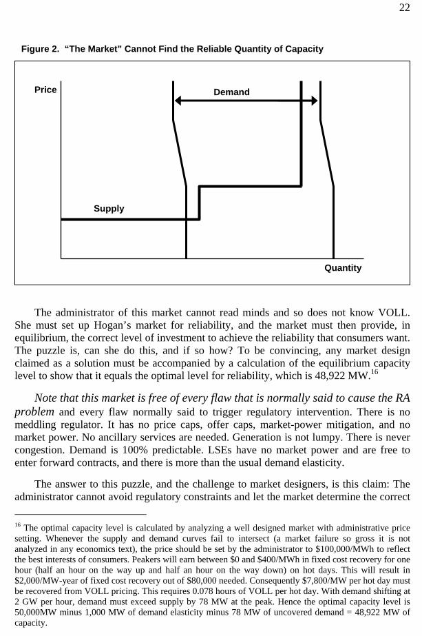
The administrator of this market cannot read minds and so does not know VOLL. She must set up Hogan’s market for reliability, and the market must then provide, in equilibrium, the correct level of investment to achieve the reliability that consumers want. The puzzle is, can she do this, and if so how? To be convincing, any market design claimed as a solution must be accompanied by a calculation of the equilibrium capacity level to show that it equals the optimal level for reliability, which is 48,922 MW.16

Note that this market is free of every flaw that is normally said to cause the RA problem and every flaw normally said to trigger regulatory intervention. There is no meddling regulator. It has no price caps, offer caps, market-power mitigation, and no market power. No ancillary services are needed. Generation is not lumpy. There is never congestion. Demand is 100% predictable. LSEs have no market power and are free to enter forward contracts, and there is more than the usual demand elasticity.

The answer to this puzzle, and the challenge to market designers, is this claim: The administrator cannot avoid regulatory constraints and let the market determine the correct 16 The optimal capacity level is calculated by analyzing a well designed market with administrative price setting. Whenever the supply and demand curves fail to intersect (a market failure so gross it is not analyzed in any economics text), the price should be set by the administrator to $100,000/MWh to reflect the best interests of consumers. Peakers will earn between $0 and $400/MWh in fixed cost recovery for one hour (half an hour on the way up and half an hour on the way down) on hot days. This will result in $2,000/MW-year of fixed cost recovery out of $80,000 needed. Consequently $7,800/MW per hot day must be recovered from VOLL pricing. This requires 0.078 hours of VOLL per hot day. With demand shifting at 2 GW per hour, demand must exceed supply by 78 MW at the peak. Hence the optimal capacity level is 50,000MW minus 1,000 MW of demand elasticity minus 78 MW of uncovered demand = 48,922 MW of capacity.

Supply

Demand Price

Quantity

Figure 2. “The Market” Cannot Find the Reliable Quantity of Capacity

23

level of reliability. It is impossible. Not only is it impossible, but no pure-market design can be demonstrated to guide the investment level to any level near the optimal capacity level. All pure market designs for the described market fail utterly, because they can obtain no hint of consumer’s preferences regarding reliability. The market has no way of finding that VOLL is not $500 or is not $5,000,000/MWh. Every pure market design leaves the market clueless concerning the optimal level of reliability.

Of course, this market is flawed. In an unflawed market the answer would be extremely simple, either (1) just allow bilateral trading, or (2) just collect the bids, set price by intersecting the supply and demand curves, and send out the bills. Disconnect those who do not pay.

Since all other flaws have been eliminated, the lack of a market solution must be due to the two Demand-Side Flaws, which are present in this example and will be present in real markets for several years to come.

Demand-Side Flaws (Stoft 2002, p. 15)

Flaw 1: Lack of metering and real-time billing Flaw 2: Lack of real-time central control of power flow to specific customers

Elimination of either flaw would allow the investment problem to be solved, but the solution differs depending on the flaw eliminated. To understand why these two flaws block the two possible solutions, a deeper understanding of the investment problem is required.

In normal markets of all kinds, when there is too little productive capacity, prices are high. When there is too much capacity, prices are low. Since high prices encourage investment and low prices discourage it, commodity prices control investment. Economics shows that in competitive markets, commodity prices, electricity prices in the present case, will signal the right level of investment and the right, or adequate, level of installed capacity.

But what does “right level of capacity” mean in a normal market? It does not mean optimal reliability, because normal markets have no reliability problem. They are perfectly reliable. In a normal market, price keeps supply and demand equal and the markets are much less fragile. In a normal market, the supply curve always intersects the demand curve. The right level of capacity is the level that makes the marginal value of product to consumers equal the long-run marginal cost of production. No economics text will explain how a market sets capacity to the adequate level for reliability, because normal markets cannot do that and do not need to.

One way to solve the reliability problem would be to eliminate it the way it is eliminated in a normal market—by having price equilibrate supply and demand. In a power market, this would mean that when the ISO needed to shed load, as it now does in a rolling blackout, it would simply step the price up by perhaps $500/MWh, and this would trigger quick load reductions by large consumers who would have price-controlled circuit breakers or other quick-response methods. Since these consumer actions would be voluntary, this is not involuntary load shedding. This represents the elimination of Flaw

24

#1 and the development of sufficient demand elasticity. This is the most desirable market-based solution to the reliability problem—market-provided perfect reliability.17 As demand elasticity increases, so will reliability and at some point we will be close enough to drop the concept of planned reserves, but not for a while. (See also FAQ 8 in Appendix 2.)

The other way to solve the problem, which is less efficient and requires more capacity, is to use the market to induce load to buy excess capacity. This would be a true reliability market. This way, the reliability problem still exists, and there is still highly-inefficient, involuntary load shedding. When load shedding is required, the customers with insufficient energy contracts, or with contracts whose suppliers are not performing, are cut off.

An actual reliability market requires even more infrastructure. To cut off individual customers with inadequate contracts, the ISO must know everyone’s contract position, and which units they are contracted with, and must have the ability to cut them off by remote control without affecting their neighbor. This will induce all customers to purchase long-run contracts up to the point where the cost of more contract cover is no longer worth the extra reliability they gain.18

Joskow and Tirole (2006) show that such a scheme could produce an efficient reliability market, but could this possibly be what Hogan and other energy-only advocates have in mind when they say “There could be a market for reliability but the regulatory constraint prevents its operation.” (Hogan 2005, p. 24) Could the regulatory constraint they complain of be preventing a market for individual reliability levels provided by remote-controlled individual blackouts? It does not seem possible that energy-only advocates have this in mind. Instead, they must be imagining one of the energy-only designs in which all customers receive the same reliability level.

But an efficient market for uniform reliability is even more impossible than an efficient market for individual reliability. The later could be achieved with new sophisticated market infrastructure. But an efficient market for uniform reliability is impossible no matter what the infrastructure. If reliability is not individualized then individuals know that they will not receive less reliability if they pay less for it, because they can be given less only if everyone is given less. Consequently, everyone will refuse to pay for collective reliability and all will attempt to enjoy a free ride.

An important point concerning any reliability market is that end-use customers, and not LSEs, must decide their own contract level. That is the only legitimate market signal for reliability. If LSE’s are deciding, they will base their decisions not on consumer preferences but on the penalties that will be imposed by regulators if they provide too

17 Perfect reliability in the context of the adequacy problem means that there will be no blackouts caused by inadequate installed capacity. It does not mean lightning will never strike a power line and put your lights out. 18 For completeness, a related solution, still blocked by Flaw 2, would be to have LSEs choose their reliability level, and customers chose their LSE on the basis of the reliability and cost. This is impossible because neighbors cannot yet be given different reliability levels even if they sign up with different LSEs.

25

little reliability. That would leave central administrators, and not the market, in charge of the reliability and capacity levels.

In summary, perfect reliability (with regard to the adequacy problem) could be achieved by eliminating Flaw 1. An individual reliability market could be achieved by eliminating Flaw 2. An efficient uniform reliability market, as promised by energy-only advocates, cannot be achieved under any circumstances. Consequently, the market administrator will determine the level of installed capacity either inadvertently or with a resource-adequacy program. At this time, there is no other choice.

26

7. The “Energy-Only” Approach There is no pure market solution to the RA problem, yet energy-only approaches and long-term-contract approaches frequently imply that they are just that, pure-market solutions, perhaps with a few administrative features in the ancillary service market (Hogan 2005).19 This discrepancy in claims deserves a clear resolution. Fortunately the clarity of Hogan’s 2005 paper, “On an ‘Energy Only’ Electricity Market Design for Resource Adequacy,” provides a unique opportunity to resolve this debate.

Hogan’s paper advances the view that a capacity-market approach would overturn the electricity market while an energy-only approach could and should leave major economic decisions surrounding investment to be voluntarily arranged by the parties. In other words, its central claim is that a market, free of central control, can solve the RA problem if an energy-only approach is used, while a capacity approach will overturn the market by allowing a central administrator to make the major economic decisions surrounding investment.

This is not correct. An energy-only approach can use the market to solve every part of the resource adequacy problem except one—adequacy. The adequacy part of the adequacy problem is the elephant in the room that energy-only approaches never address head on—because current markets cannot tell us how much capacity is needed for adequate reliability. It’s not that an energy-only market will not procure adequate capacity; the problem is that they must be designed specifically to procure adequate capacity, and the design parameters, must be set by a central authority—not the market. The planners must adjust the energy demand curve to make the market buy an adequate level of capacity rather than an inadequate or superfluous level of capacity. The market cannot adjust the all-controlling design parameters.

The Centrally-Planned Energy-Only Demand Curve Hogan presents an energy+reserve demand curve, which is controlled at every relevant point by three parameters which appear to be well planned but which did not come from any market, the price cap of $10,000/MWh and two operating-reserve parameters of 3% and 7%. These three parameters do not just fine tune the demand curve; they entirely control the missing money problem which is the central determinate of adequacy. These three parameters control the fixed cost recovery of peakers, roughly $80,000 per MW-year of capacity, and consequently they control this amount of revenue for every MW of capacity in the system.20 In a 50,000 MW system, that comes to $4 billion per year (with the parameters set properly) controlled by the centrally-planned parameters. Depending on how these parameters are set, the resource level, in other words the level of installed 19 “Similarly, the emphasis on an “energy only” market does not mean that there would be nothing but spot deliveries of electric energy with a complete absence of administrative features in the market. Since the technology of electricity systems does not yet allow for operations dictated solely by market transactions with simple well defined property rights, the system requires some rules to deal with the complex interactions in the network. To the contrary, there would of necessity be an array of ancillary services and associated administrative rules for such services.” (Hogan, 2005, p. 9) 20 Peaker fixed cost (for a Frame unit) is diversely estimated at between $60,000 and $95,000/MW-year. The value of $80,000 is used throughout this paper because it is convenient and plausible.

27

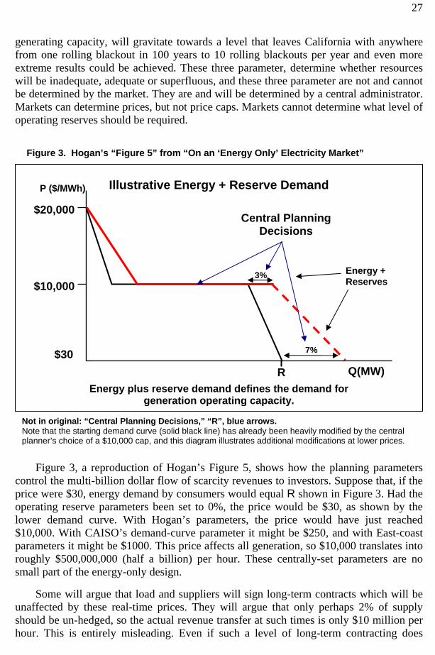
generating capacity, will gravitate towards a level that leaves California with anywhere from one rolling blackout in 100 years to 10 rolling blackouts per year and even more extreme results could be achieved. These three parameter, determine whether resources will be inadequate, adequate or superfluous, and these three parameter are not and cannot be determined by the market. They are and will be determined by a central administrator. Markets can determine prices, but not price caps. Markets cannot determine what level of operating reserves should be required.

Figure 3, a reproduction of Hogan’s Figure 5, shows how the planning parameters control the multi-billion dollar flow of scarcity revenues to investors. Suppose that, if the price were $30, energy demand by consumers would equal R shown in Figure 3. Had the operating reserve parameters been set to 0%, the price would be $30, as shown by the lower demand curve. With Hogan’s parameters, the price would have just reached $10,000. With CAISO’s demand-curve parameter it might be $250, and with East-coast parameters it might be $1000. This price affects all generation, so $10,000 translates into roughly $500,000,000 (half a billion) per hour. These centrally-set parameters are no small part of the energy-only design.

Some will argue that load and suppliers will sign long-term contracts which will be unaffected by these real-time prices. They will argue that only perhaps 2% of supply should be un-hedged, so the actual revenue transfer at such times is only $10 million per hour. This is entirely misleading. Even if such a level of long-term contracting does

Q(MW)

$20,000

$10,000

Illustrative Energy + Reserve Demand

Central Planning Decisions

3%

7%

R Energy plus reserve demand defines the demand for

generation operating capacity.

Energy + Reserves

$30

P ($/MWh)

Figure 3. Hogan’s “Figure 5” from “On an ‘Energy Only’ Electricity Market”

Not in original: “Central Planning Decisions,” “R”, blue arrows.Note that the starting demand curve (solid black line) has already been heavily modified by the central planner’s choice of a $10,000 cap, and this diagram illustrates additional modifications at lower prices.

28

materialize, the cost impact on load and the revenue impact on generation will be exactly what it appears to be considering only real-time prices. This is because the price of forward contracts is affected by real-time prices. Forward prices reflect expected day-ahead prices, and day-ahead prices reflect real-time prices. If real-time prices are expected to rise to $10,000/MWh for an average of 5 hours per year, then a forward contract for a year of base-load power will cost $49,500/MW-year more than if spot price are never expected to rise above $100/MWh. Forward contracts hedge risk, but they do not cause suppliers to sell power at far less than the expected spot price. If either party sees that spot prices would be much more favorable to them than buying a forward contract, they will not sign the forward contract. Hence forward contracts reflect spot prices.

Finally, consider the parameters themselves. The 7% value for operating reserves is essentially an engineering value. Engineers were setting this for years before there were any electricity markets to speak of, and they do a good job of it. This parameter is not set by the market. But, what matters more is how rapidly price climbs when the 7% requirement is not met. Often there are proposals to calculate the appropriate price based on the chance of a blackout, and the value to load of not being blacked out. But neither of these inputs is determined by the market. The most crucial parameter is the value of lost load (VOLL). This value is often proposed for the price cap. The central reason an energy-only approach cannot use the market to determine adequacy is that the market cannot determine VOLL, and VOLL is the main determinant of how much capacity is needed to provide consumers with their desired reliability tradeoff. VOLL is the average value placed by consumers on losing power in an average rolling blackout. This average is notoriously hard to estimate, but that difficulty is not the point. The point is that it must be estimated, because the market does not and cannot determine it. Such estimates are performed by academics or planners, not markets. Planners compute a value that they believe reflects society’s needs because the current markets cannot determine the need for reliability. Of course they will take account of certain market data, regulators always do. But just because a regulator relies on his or her observations of the market when setting prices does not mean we have a free market. If the regulator sets the price, it is a regulated market.21 It is unfortunate that the market does not determine VOLL, but it does not.

Central Planning of Quantity Leaves Room for the Market Why did Professor Hogan recommend a centrally-planned method of securing adequate resources? Because he had no choice. There is no pure-market approach that makes sense. Nonetheless, markets have a tremendously important role to play in securing adequate capacity. They are needed to assure the low cost, high quality and performance of the capacity purchased. The market can select who should build, where plants should be built, the proportion of base-load plants; it can determine how many peakers should be super-quick-start aero derivatives, whether they should be dual fuel, and much more. It 21 The exception, which has caused much confusion, is an auction. The auctioneer (ISO) sets a price based entirely on bids and not on his own judgment. Consequently, an auction is the one case of a pure market price set by a (highly constrained) central administrator. There is no process remotely like an auction for determining VOLL.

29

can solve problems we are not even aware of when we design the market. In short, markets can do all the really difficult things that we need markets to do. They simply cannot tell us how much capacity we need because we never tell the market how much reliability we are willing to pay for. Markets are amazing coordinators, but they do not read minds.

Hogan is not alone in relying on central planning. Centrally determined obligations control capacity investment under Oren’s energy-only proposal.

“Once the target quantities of generation capacity are determined by engineering considerations that quantity is allocated as a prorated obligation to the load serving entities.” (Oren 2005, p. 2)

Any wholesale customer or LSE should be required to carry call options that will cover its peak load … plus adequate reserves as set by the regulator. (Oren 2005, p. 6)

The energy-only approach is advertised as the pure market-approach because its non-market mechanisms tend to be overlooked, and because the slogan “it’s the market approach” is somehow persuasive. If there were a pure market approach, that might decide the question. Since there is not, we must look deeper. In fact there are several distinct approaches that utilize the markets to make almost all the decisions except the decision of what is the adequate resource level.

To chose between these approaches, we must look at their performance in several dimensions. Although all can hit any desired adequacy target on average, some will miss the target by more on both the high and low side. Some will raise risk premiums more than others, a problem that could easily cost consumers dearly. Market power is an equally important consideration. Simplicity and durability are also crucial.

In selecting an approach, there is one pitfall to avoid above all others. If a design is picked that appears to allow the market to determine adequacy, it will almost certainly fail. That is because the market cannot determine what is adequate, and such a design will inhibit the necessary regulatory determination because the levers of control will be obscure. That has led to an absence of any coherent control of adequacy in the past, and is likely to lead to disaster in the future. Better to admit the regulator has a hard and necessary job and face the task squarely. As will be demonstrated shortly, this is not such a formidable assignment—partly because we know a fair amount about what is adequate, and partly because a 5% error in targeting causes less than a 1% retail cost increase. Even a good market could not do much better—there is just not that much room for improvement. What is important is not to leave adequacy to chance and not to cause damaging side effects by preventing the market from doing what we need it to do—control quality and performance.

In summary, the energy-only approach relies on an administratively determined energy+reserve demand curve to control scarcity revenues, investment, and capacity level. It is no less centrally planned than the ICAP approach.

30

8. Replacing the Missing Money The central problem of resource adequacy was defined above as missing money. This has been documented by all of the Eastern ISOs, which explains their continued use of capacity markets designed primarily to replace missing revenues. Perhaps Joskow has made the most systematic study of this problem.

On the one hand, a market response that leads prices (adjusted for fuel costs) and profits to fall and investment to decline dramatically when there is excess capacity, is just the response that we would be looking for from a competitive market. … At least some of the noise about investment incentives is coming from owners of merchant generating plants who would just like to see higher prices and profits. On the other hand, numerous analyses of the performance of organized energy-only wholesale markets indicate that they do not appear to produce enough net revenues to support investment in new generating capacity in the right places and consistent with the administrative reliability criteria that are still applicable in each region. (Joskow 2006, p. 15)

Joskow has not forgotten that oversupply leads to low prices, yet he still reports that “wholesale markets … do not appear to produce enough net revenue,” and he is including revenue from ICAP markets as well as energy markets.

However, even adding in capacity revenues, the total net revenues that would have been earned by a new plant over this six year period would have been significantly less than the fixed costs that investors would need to expect to recover to make investment in new generating capacity profitable. This phenomenon is not unique to PJM. Every organized market in the U.S. exhibits a similar gap between net revenues produced by energy markets and the fixed costs of investing in new capacity measured over several years time (FERC (2005), p. 60; New York ISO (2005), pages 22-25). There is still a significant gap when capacity payments are included. (Joskow 2006 p. 16).

What is the proximate cause of these shortfalls? For our purposes, the relevant ones are those that depress energy market revenues, and Joskow provides the most complete list.

The problems include: [1] price caps on energy … [2] market power mitigation mechanisms that do not allow prices to rise high enough during conditions when generating capacity is fully utilized … [3] actions by system operators that have the effect of keeping prices from rising fast enough and high enough to reflect the value of lost load … [4] reliability actions taken by system operators that rely on Out of Market (OOM) calls on generators that pay some generators premium prices but depress the market prices paid to other suppliers, … [5] payments by system operators to keep inefficient generators in service due to transmission and related constraints rather than allowing them to be retired or be mothballed, … [6] regulated generators operating within a competitive market that have poor incentives to make efficient retirement decisions, depressing market prices for energy. (Joskow 2006, p. 17)

31

Although the missing money problem has been widely recognized in the Northeast, it has not been recognized frequently in the rest of the country. Two recent exceptions are the CPUC’s August 2005 Report and Hogan’s report to the CAISO.

The primary purposes of the Commission’s RA requirements are: (1) to ensure sufficient incentives for new electric infrastructure investment, and maintenance of necessary existing generation, by providing a revenue stream that is missing from today’s capped energy markets to compensate generation owners for their fixed costs. (CPUC 2005, p. 1)

The missing money problem arises when occasional market price increases are limited by administrative actions such as price caps. … these administrative actions reduce the payments that could be applied towards the fixed operating costs … The resulting missing money reduces the incentives to maintain plant or build new generation facilities. (Hogan 2005, p. 1)

The most convincing study may have been done by ISO-NE which went back 18 years to look at shortage hours (see Figure 6). Given the ISO’s real-time pricing policies, there were not enough shortage hours in any of those 18 years to cover the fixed costs of a peaker. Because the missing money problem is central to resource adequacy, it is worth looking closely at the two ways it can be solved, with capacity obligations and with high spot prices, and at why other approaches do not attempt to solve it.

The ICAP Approach The simplest way to replace the missing money is the classic capacity market. All load is required to buy its proportional share of capacity credits so that the total capacity purchased equals the adequacy target. All installed capacity is allowed to sell capacity credits equal to its nameplate capacity. This is enforced by charging load something like $150,000 per MW-year of shortfall below its capacity requirement. If there is less than adequate capacity, some load will inevitably fall short and be fined. Suppliers, recognizing the need of load to avoid fines, will raise the price of their capacity credits to $150,000/MW-year, so even though the market is only a little short of capacity and only a little money is paid in fines, all capacity will receive a price of $150,000/MW-year. This is the result of the law of one price (Jevons 1879).22 Whenever the market is short of capacity, investors will find investment profitable, and this will bring installed capacity up to the target level. If it exceeds the target, the price (barring market power) will fall to zero and investment will cease.23 Capacity payments will average something between $0 and $150,000/MW-year and their actual average will be just enough to restore the missing money and make investors whole.

22 “In the same open market, at any moment, there cannot be two prices for the same kind of article.” From The Theory of Political Economy. 23 Actually, the investment process is rather more complex because investors build on the basis of anticipated ICAP payments as well as other revenues and costs over the life of the plant.

32

Hogan’s Energy-Only Approach Hogan adopts the spot-price approach to restoring the missing money. He suggests raising the offer-cap in the spot market to something like $10,000/MWh, and requiring the ISO to raise spot prices towards this level as operating reserves fall in real time. So, with operating reserves of about 5%, the spot price might reach $5,000/MWh. This will certainly increase the average level of installed capacity. If the administratively determined energy demand curve is properly designed, it will induce on average the same target capacity that the ICAP approach induces. Determining what parameters will induce what capacity level is not as easy as it is with the capacity approach.

If, at the adequate level of capacity, the demand curve causes spot prices that are high enough on average for a peaker to just cover its fixed costs, then to a good approximation, the market will induce the right level of installed capacity. For the administrator to set the demand parameters correctly, it is necessary to calculate the distribution of price spikes that will be induced by load fluctuations, generator outages, and transmission outages. This is quite a difficult calculation. First one must calculate the target capacity level, just as in the ICAP approach, and then, for that level, one must compute the frequency and duration of shortage events that occur for only a few hours per year and depend on extremely unusual and anomalous conditions.

But Hogan argues against this indirect route, and for what he calls “the direct determination of the willingness to pay for operating reserves.” The flat part of the curve would be determined by the administrative estimate of VOLL, but the steeply sloped part at the right, should be determined by the benefit of operating reserves.

If the operating reserve demand curve captures the value of reliability, the resulting expected equilibrium loss of load probability should be the standard. This stands in contrast to an alternative approach that would fix the installed capacity requirement and determine the operating reserve demand to produce enough revenue to support investment that would meet the installed capacity target. … The indirect route of specifying the expected loss of load probability [which is how the capacity target is determined] should not replace the direct determination of the willingness to pay for operating reserves. (Italics added.) (Hogan 2005, p. 22)

This approach requires the administrator to directly determine the willingness of consumers to pay for operating reserves. The market will not directly determine this, as consumers do not shop for operating reserves. Consequently, the determination will necessarily be made by a market administrator (with help from an engineer) who will capture the value of reliability which is determined from the administratively determined estimate of VOLL. Unfortunately, even if the administrative determination of VOLL were completely accurate, determining the value of operating reserves would still need to rely on a theory of valuing reserves not yet developed.

The direct approach requires the administrator to determine VOLL. Some idea of the difficulty of this determination can be gained from the results obtained in the past. Bushnell (2005) tells us that “Most surveys put the ‘value of lost load’ between $2000/Mwh and $50,000/Mwh.” Hogan suggests the geometric mean of the range,

33

$10,000/MWh, but engineers seem to have a different view. Their view may simply be wrong, or it may implicitly account for some intuitive concern about the danger of cascading outages when the system is short of supplies. Their estimate can be backed out of their required loss of load probability, one event in 10 years, the estimated length of the event, three hours, and the fixed cost of a new peaker, $80,000/MW-year. The required relationship is: FCP = Blackout Hours per Year × VOLL. which implies the engineering VOLL = ($80,000/MW-year) / (0.3 h/year), which is $266,666/MWh.

Whether the more practical indirect approach is used to administratively determine the energy demand curve, or the administrator uses Hogan’s method of direct determination, the spot-price approach will restore enough missing money to induce a higher level of installed capacity. With the indirect approach, it should induce a resource level near the standard reliability-based capacity target, and with the direct approach, some level implied by the administrator’s estimate of VOLL and the operating reserve parameters.

Other Energy-Only Approaches Ignore the Missing Money Generally, energy-only approaches simply ignore the missing money problem for one of two reasons. They either assume that it will be fixed by the regulator, for example by the CPUC, or they propose an alternative cause of the missing money that requires no special attention by the RA mechanism. Consider first the role of the regulator.

Under an energy-only approach that specifies an obligation on the part of load to purchase options, the PUC could play one of two roles. It could either specify a obligation level for each LSE and a penalty for failing to meet the obligation, or it could simply purchase the options itself and force the LSEs to pay for their shares. Assuming that in the first case the PUC has set the penalty high enough to force compliance, there will be no difference in the quantity of options purchased and no difference in the price paid between the two methods.24 Because of the equivalence of these two approaches, and because bilateral contracting is frequently assumed, we will discuss the energy-only proposals under the assumption that a penalty will be imposed for non-compliance.25

When an energy-only approach fails to give any guidance on the need for penalties or discourages their use in favor of simply emphasizing the benefits of options, the PUC may conclude that penalties are unnecessary and choose to avoid them entirely. But this can only result in resource adequacy by coincidence, and the studies by Joskow and the Eastern ISOs imply such a coincidence would be entirely unexpected. A zero penalty— 24 This ignores transaction cost and market power differences, which are second order effects, and likely more problematic under a bilateral approach. Even if a more general penalty structure is required, it can be accomplished with either approach. For example, if the PUC has determined that it will purchase 50 GW if the option price is $X but only 49 GW if it is $2X, it could achieve the same outcome in a bilateral market by imposing a penalty of $X on LSEs that did not buy their share of 50 GW, and of $2X on LSEs that did not buy their share of 49 GW. 25 In contrast, ISO-NE and PJM will actually purchase the forward contracts and charge each LSE its share.

34

that is, no enforcement of the obligation—is appropriate only if the combination of price caps, operating reserve payments, and load duration curve results in covering the fixed costs of a peaker when the capacity is at the level deemed adequate for reliability.

By failing to give guidance on the target and penalty, the actual solution of the adequacy part of the RA problem is sidestepped and left to the regulator. For example, suppose $60,000/MW-year is missing at the target level of capacity. If the regulator chooses a non-compliance penalty of $20,000/MW-year, LSEs will fail to meet their obligation even though the energy-only approach is carried out to the letter. In other words, if option strike prices are selected appropriately and obligations are targeted correctly, that does not guarantee a solution to the adequacy problem, without a proper penalty structure.

Alternatively, energy-only approaches may be implicitly assuming that the regulator will set an obligation level and use an extremely high penalty, such as $600,000/MW-year in the above example. Admittedly, we see no indication of this in the penalty language of the reviewed papers. However, this would fit with the view that the regulator does not need any economic advice regarding how to achieve an adequate capacity level. The regulator would simply have the engineers set the target and then enforce the purchase of physical options, up to that level, with a penalty that was sure to induce compliance. Unfortunately, as Chao and Wilson (2004) and Hogan and Harvey (2000) point out, forcing load into high levels of forward contracting shifts market power from the spot market to the forward market. An extremely high penalty backing an imposed vertical demand curve could cause severe problems. If the requirement includes a lead time of three to four years as in the ISO-NE design, market power in the forward market will be mitigated by new entry, but as discussed later, market power problems are non-trivial even in this case.

Energy-only designs without High Spot Prices have so far failed to address the economic mechanism by which adequacy is achieved. Instead Chao and Wilson (2004) and others provide valuable insights into how to manage risk in the investment market and how to control market power in the spot market without interventionist mitigation measures. Both of these insights should be applied to any RA design.

Although some authors leave the targeting and enforcement of obligations as a detail for the regulator, still others ignore or minimize this issue, because they propose a different cause for the investment shortfall, other than missing money. Unlike the documentation of the missing-money problem by the Northeast ISOs, and by Joskow, these other causes are not well documented.

Other contributions to the energy-only design track include Wolak (2004) focusing on the importance of long-term contracting, Chao and Wilson (2004) focusing on options and risk management, and Bidwell (2005), Bidwell and Henney (2004), and Oren (2005) focusing on options. The authors make helpful contributions by highlighting some element of the resource adequacy problem and some part of the solution, but generally the approaches pay little attention to the possibility that spot-prices are systematically too low.

35

The contract adequacy approach The contract adequacy approach imposes a regulatory requirement on load to purchase long-term energy contracts. It was originally developed as a method of controlling market power and serves that purpose better than the more popular market mitigation measures.26 In more recent years it has also been proposed as a method for assuring resource adequacy, but this requires a fresh analysis.

Proponents of this approach hold that the source of the investment problem is not missing money but the lack of long-term contracts for new investors. Call this the missing-contract problem. In other words, if a new investor could lock in the expected spot price for some years in advance of construction, the investor would be willing to build in today’s market. In contrast, missing money refers to low spot prices and not to a failure to lock in spot prices with a long-term contract. The following is one explanation of the missing-contract view.

So how do the successful markets described earlier ensure that sufficient generation capacity is available to meet current and future demand without a capacity market? They do it the same way as other industries … through an active forward market. For example, jet aircraft and jet aircraft engines are typically sold on a forward market, far in advance of the delivery date. (Wolak 2004, p. 4)

This explanation asserts that other industries that require long-term capital investments rely on long-term forward contracts for their products as the basis for building production capacity. A host of common examples argue otherwise. Hotels can be more expensive than most generators, yet few rooms are booked before an investor breaks ground on a new Hotel. General Motors sells no long-term contracts for cars before it builds the factory to produce them. Chip manufactures build chip fabricating plants before the chips are even designed let alone sold. Long-term investments are rarely financed on the basis of long-term product sales; and long-term investments are often made in industries that sell almost all of their product only a month or two in advance.

Why do investors in other industries invest in assets with lives of 10 to 60 years when they have sold none of the output from their investment? Because, they expect to sell product at profitable prices. Investments are almost always based primarily on expectations, not on the basis of locked-in forward contracts.

This makes expectations crucial, and the electricity industry has a special problem with investor expectations because of regulatory risk. This requires either the reduction of regulatory risk, or the use of long-term contracts. In either case the missing money must be replaced. In some venues a short-term capacity market that is broadly accepted might reduce regulatory risk sufficiently. But given the present regulatory climate it may be best to implement a long-term capacity market which both reduces regulatory risk and provides investors with moderately long contracts.

26 Long-term contracts curb market power because raising the spot price is not profitable for a supplier who has already sold its power in the forward market.

36

The option portfolio approach An option portfolio approach has been proposed as a method for a utility’s risk management in wholesale markets. This approach utilizes an annual auction of a specified quantity of multi-year option contracts on physical capacity with a specified range of strike prices. Note that the specification of physical capacity contracts is a major step towards convergence with the ICAP approach. This approach has been shown by Chao and Wilson (2004) to have beneficial effects on risk management and to transfer market power to the forward option market.

The fundamental deficiency of monthly ICAP and ACAP markets is that they do not transfer negotiations to forward markets for long-term contracts where the effects on resource adequacy are greater because of the greater elasticity of supply from capacity expansion and new entry. (Chao and Wilson, 2004)

This insight into the role of long-term contracts supports the need for convergence and the inclusion of options, or equivalently the subtraction of SRShare, in the recent New-England designs.

As with other approaches, it is necessary to impose an obligation on load to purchase some type of contract in order to achieve resource adequacy. In the option portfolio approach, the aggregate demand for options is determined by the “obligations of the LSEs to satisfy their resource-adequacy obligations specified by the PUC” (Chao and Wilson 2004). As with other energy-only approaches there has as yet been no specification of the form or magnitude of this obligation, something that is left to the PUC.

The option portfolio approach can assure resource adequacy if the load obligation is as forceful as the obligation in a forward capacity market design. It must target an adequacy level compatible with reliability standards, and it must enforce this with some penalty roughly equivalent to an ICAP or FCM demand curve. If this is done in present markets, the missing money would be replaced by load paying more than the actuarial value of the options obtained. Option prices would be largely determined by the value of avoiding administrative penalties. However this mechanism has not yet been brought within the purview of the option-portfolio approach.

The call-option obligation approach The call-option obligation approach, like the option-portfolio approach, suggests that load be obligated to purchase options with various strike prices. As its name suggests, it puts more emphasis on the load obligation. But also like the option-portfolio approach, it does not specify how the quantity obligated or the strength of the obligation should be determined. In fact it is noted that “the options will be ‘out of the money’ most of the time and hence their cost will be relatively low.” (Oren 2005) This appears to suggest that the options are not made expensive by high penalties backing obligations that force load to pay more than the option’s value. This approach to assuring generation adequacy is instead based on the concepts of risk management and risk sharing arrangements “when needed hedging practices are falling

37

short due to market imperfections and the regulatory interventions.” (Oren 2005) These concepts of risk management have been discussed in the California context which has a relatively low price cap of only $250. Although a low cap is a classic source of missing money, that is not the source of the problem pointed to by risk-management approaches.

When electricity prices are artificially suppressed by a low cap as in California (currently $250/MWh) the call option value is also depressed due to limited price volatility. Hence selling call options may not generate sufficient income to support investment in generation capacity. It would make sense in such an environment to set the strike price to the level of the current cap and raise the offer cap on generators that do not sell call options. (Oren 2005)

This explanation begins with limited price volatility caused by the cap. Volatility is the source of risk and consequently volatility makes risk management, and hence options, valuable. The more risk, the more valuable the option. A low price cap takes away option value by taking away risk. Hence selling call options generates less income in the less risky, low-cap environment. This explains why the options are often interpreted as insurance for load against price volatility. “The call option acts as price insurance.” (Oren 2005)

However there is a problem with the final step in the explanation. While raising the cap would increase risk to consumers and thereby induce them to spend more money on insurance (options), this will not translate into more profit for the insurers (generators) if the insurance industry is competitive. In a competitive industry, the cost of insurance is held down to the cost of providing the insurance (plus a normal rate of return) which will be greater in a riskier environment. Hence, if the generators are competitive providers of insurance to load, increasing the risk to load will increase the cost of insurance and the income of generators, but it will not increase their profits. Instead, their increased revenues will simply cover their increased costs. Increased income that simply covers increased costs, without increasing profits, will not support or induce any additional investment in new capacity. Only if suppliers have monopoly power in the price-spike insurance market will imposing higher, riskier prices on load result in increased profits and increased investment.

This should not be taken as a criticism of a call option obligation. In fact that is central to the convergent design advocated here. The conclusion should be that more attention needs to be given to the obligation aspect of option obligations. In a market with spot prices that are too low to induce adequate investment, a strong and well targeted obligation is required. It must target an adequate level of installed capacity and be backed by a penalty sufficient to induce load to pay enough extra for the options to replace the money that is missing due to low spot prices.

The Reliability-Option Approach The reliability option approach (Bidwell 2005; Bidwell and Henney 2004) is an option-based ICAP approach and illustrates how close the ICAP and energy-only approaches are once options are added to the ICAP approach along with strongly enforced obligations. Like the other two call-option approaches, this one uses options that are both financial

38

and physical. Because it uses a capacity target and buys physically based options up to that target level, the price of these options will be driven up to the point where adequate new entry occurs. This will force the cost of options to levels well above their option value and thereby restore the missing money.

In summary, ICAP approaches replace the missing money and restore adequacy as does Hogan’s energy-only approach. All previous energy-only approaches ignore the missing money and focus on risk management or market power reduction. However, if they expand their obligation components to become the driving force behind option prices they can transfer the appropriate level of missing money. Once this is done, and the obligation is targeted at the reliable level of installed capacity, the energy-only approaches will be nearly equivalent to the ICAP approaches that include options.

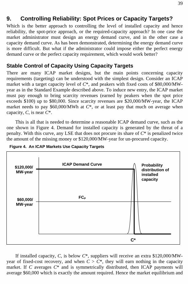
39

9. Controlling Reliability: Spot Prices or Capacity Targets? Which is the better approach to controlling the level of installed capacity and hence reliability, the spot-price approach, or the required-capacity approach? In one case the market administrator must design an energy demand curve, and in the other case a capacity demand curve. As has been demonstrated, determining the energy demand curve is more difficult. But what if the administrator could impose either the perfect energy demand curve or the perfect capacity requirement, which would work better?

Stable Control of Capacity Using Capacity Targets There are many ICAP market designs, but the main points concerning capacity requirements (targeting) can be understood with the simplest design. Consider an ICAP market with a target capacity level of C*, and peakers with fixed costs of $80,000/MW-year as in the Standard Example described above. To induce new entry, the ICAP market must pay enough to bring scarcity revenues (earned by peakers when the spot price exceeds $100) up to $80,000. Since scarcity revenues are $20,000/MW-year, the ICAP market needs to pay $60,000/MWh at C*, or at least pay that much on average when capacity, C, is near C*.

This is all that is needed to determine a reasonable ICAP demand curve, such as the one shown in Figure 4. Demand for installed capacity is generated by the threat of a penalty. With this curve, any LSE that does not procure its share of C* is penalized twice the amount of the missing money or $120,000/MW-year for un-procured capacity.

If installed capacity, C, is below C*, suppliers will receive an extra $120,000/MW-year of fixed-cost recovery, and when C > C*, they will earn nothing in the capacity market. If C averages C* and is symmetrically distributed, then ICAP payments will average $60,000 which is exactly the amount required. Hence the market equilibrium and

ICAP Demand Curve $120,000/MW-year

C*

$60,000/MW-year

FCP

Probability distribution of installed capacity

Figure 4. An ICAP Markets Use Capacity Targets

40

average capacity level will be C*. If scarcity revenue has been misestimated, the equilibrium will be off by a little. For example if scarcity revenues are actually $40,000 instead of $20,000/MW-year, investors will build capacity to the point where the ICAP payments average only $40,000/MW-year. This means they will be $120,000 one-thirds of the time and $0 two-thirds of the time. If the capacity distribution is normal, that means equilibrium C will be above the target by 0.43 standard deviations. Typical distributions of capacity have been found to have standard deviations near 5% of target capacity, so if scarcity revenues are mistakenly under-estimated by $20,000/MWh, half of their actual value, installed capacity will miss its target value by about 2%.

Erratic Control with Spot Energy Prices Three problems must be overcome for the price-based control of installed capacity to function accurately. (1) VOLL must be estimated. (2) The energy demand curve must be administratively set based on VOLL and observable system characteristics. (3) The market must forecast profitability accurately from historical prices. The first two problems are the administrator’s and were discussed previously; the third is the market’s problem and will be addressed here.

Once Hogan’s energy+reserve demand curve has been administratively set, how will investors respond? They will understand that when the capacity level is low the market will cover more of their fixed costs, and when there is excess capacity it will cover less, just as with the ICAP demand curve. This relationship may be called the energy-only capacity demand curve since it relates scarcity revenue to capacity level just as the ICAP demand curve relates ICAP payments to capacity level. This curve is never calculated by proponents of an energy-only market, but it is the curve that matters to investors. It tells them how profitable they will find the market at various capacity levels. Their estimate of this curve will determine when they invest. They will not invest when the market appears to be heading into the low region of the energy-only capacity demand curve. However, if the energy-only capacity demand curve indicates the expected capacity level will provide generous scarcity revenues, they will invest.

Energy-only market designs do not include the energy-only capacity demand curve for two reasons. The practical reason is that it is very difficult to calculate. The theoretical reasons is that, if VOLL has been estimated correctly and the energy+reserve demand curve designed correctly, economic theory assures the administrator that the market should build the right amount of capacity. But, the investor does not care about this assurance and is simply concerned with what investment levels are profitable. Because a theoretical calculation of the energy-only capacity demand curve is nearly impossible, the investor will want to observe actual market prices and use them to estimate this curve. What should they expect to see in the market?

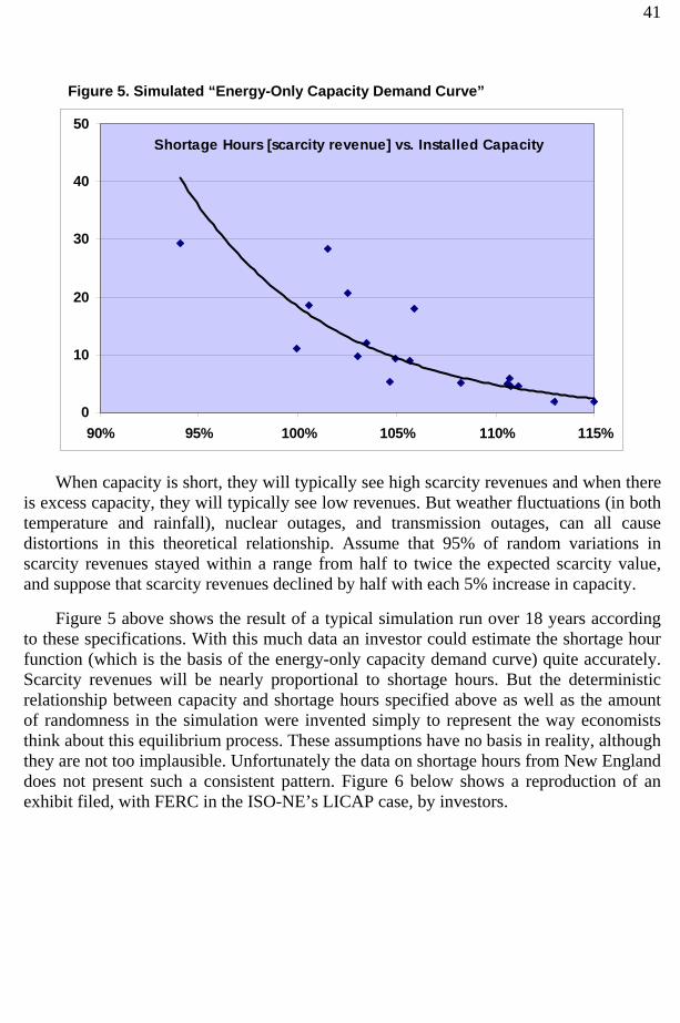
41

When capacity is short, they will typically see high scarcity revenues and when there is excess capacity, they will typically see low revenues. But weather fluctuations (in both temperature and rainfall), nuclear outages, and transmission outages, can all cause distortions in this theoretical relationship. Assume that 95% of random variations in scarcity revenues stayed within a range from half to twice the expected scarcity value, and suppose that scarcity revenues declined by half with each 5% increase in capacity.

Figure 5 above shows the result of a typical simulation run over 18 years according to these specifications. With this much data an investor could estimate the shortage hour function (which is the basis of the energy-only capacity demand curve) quite accurately. Scarcity revenues will be nearly proportional to shortage hours. But the deterministic relationship between capacity and shortage hours specified above as well as the amount of randomness in the simulation were invented simply to represent the way economists think about this equilibrium process. These assumptions have no basis in reality, although they are not too implausible. Unfortunately the data on shortage hours from New England does not present such a consistent pattern. Figure 6 below shows a reproduction of an exhibit filed, with FERC in the ISO-NE’s LICAP case, by investors.

Figure 5. Simulated “Energy-Only Capacity Demand Curve”

Shortage Hours [scarcity revenue] vs. Installed Capacity

0

10

20

30

40

50

90% 95% 100% 105% 110% 115%

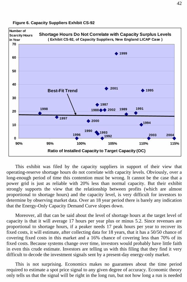
42

This exhibit was filed by the capacity suppliers in support of their view that operating-reserve shortage hours do not correlate with capacity levels. Obviously, over a long-enough period of time this contention must be wrong. It cannot be the case that a power grid is just as reliable with 20% less than normal capacity. But their exhibit strongly supports the view that the relationship between profits (which are almost proportional to shortage hours) and the capacity level, is very difficult for investors to determine by observing market data. Over an 18 year period there is barely any indication that the Energy-Only Capacity Demand Curve slopes down.

Moreover, all that can be said about the level of shortage hours at the target level of capacity is that it will average 17 hours per year plus or minus 5.2. Since revenues are proportional to shortage hours, if a peaker needs 17 peak hours per year to recover its fixed costs, it will estimate, after collecting data for 18 years, that it has a 50/50 chance of covering fixed costs in this market and a 16% chance of covering less than 70% of its fixed costs. Because systems change over time, investors would probably have little faith in even this crude estimate. Investors are telling us with this filing that they find it very difficult to decode the investment signals sent by a present-day energy-only market.

This is not surprising. Economics makes no guarantees about the time period required to estimate a spot price signal to any given degree of accuracy. Economic theory only tells us that the signal will be right in the long run, but not how long a run is needed

Shortage Hours Do Not Correlate with Capacity Surplus Levels( Exhibit CS-92, of Capacity Suppliers, New England LICAP Case )

1987

1995

2000 1994

20042003199219931990

1996

2002

1997

1998 1988

2001

1999

1989 1991

0

10

20

30

40

50

60

70

90% 95% 100% 105% 110% 115%

Ratio of Installed Capacity to Target Capacity (OC)

Number of Scarcity Hoursin Year

Best-Fit Trend

Figure 6. Capacity Suppliers Exhibit CS-92

43

to read the signal accurately. There are several reasons the ISO-NE data may be more realistic than the hypothetical data of Figure 5. First, engineering estimates of the steepness of a blackout-hours curve shows that these fall by half for each 2.2% increase in capacity, but shortage hours, which are at least 50 times more prevalent, fall off much more gradually. So the shortage-hour curve is probably much flatter than assumed in Figure 5. Second, many shortage hours are caused by security problems and these are even less related to installed capacity. This again tends to flatten the energy-only capacity demand curve. Furthermore, the ISO-NE data indicates that year-to-year variability in shortage hours is greater than assumed. Taken together, even these few considerations suggest that the ISO-NE data paints a more realistic picture.

Some will argue that long-term contracts will solve this problem. But the signers of long-term contracts can read the spot price average no better than anyone else. Plants will sometimes be built, but there is little hope of a tight distribution of the installed capacity level around the true equilibrium value. That would require investors to learn things from the market in a few years that a statistician cannot deduce after decades.

In summary, installed capacity and hence reliability can be controlled by (1) using a capacity (quantity) target or (2) by administratively controlling the spot-price level. The capacity target approach is simple and reliable. The spot-price-control approach is complex and provides erratic control.

44

10. Spot Energy Prices Make the Best Performance Incentives Spot prices are far better than standard capacity payments when it comes to sending performance signals. In fact, the original ICAP payments based on nameplate capacity sent no performance signals at all. This led to basing payments on “unforced” capacity, which is capacity de-rated by its “EFORd” score. This score takes account of forced outages for which there is no excuse, but the list of excuses, like the EFORd formula itself, is arcane. During a recent cold snap in New England that saw 10,000 MW (out of 30,000) forced out of service, the average EFORd rating in New England declined by only 0.2%. That would result in a 0.2% loss of the annual ICAP payment. Because this formula is arcane and the data used in its evaluation is self reported, EFORd is widely gamed. Recently NYISO reduced its total unforced capacity by 700 MW to correct for gamed EFORd values.

Unlike the administrative and gamable EFORd formula, spot energy prices send strong performance signals with no loopholes. If a supplier misses three of a year’s thirty shortage hours, it misses nearly 10% of the year’s scarcity revenue. But one need not examine the details of spot price incentives to understand why they are the right solution to the performance problem. Economic theory recommends competitive prices exactly because they send all the right signals, the right signals to consumers, the right signals to existing capacity for performance, and the right signals to investors to build the right type and quality of capacity. In fact, if there is one central point of economic theory, it is that competitive prices provide the best performance incentives, and schemes that do not closely mimic them, generally provide poor incentives. This is the main reason economics recommends using a market approach.

Since the source of the missing money problem is price suppression (of various types), we know that performance/quality signals have been suppressed. The obvious remedy is to restore the suppressed prices. The only drawback is the concomitant restoration of market power and increased risk, but these can be controlled by hedging load, as will be discussed shortly.

Why Value-Reflective Prices are Irreplaceable There is a strong tendency in ICAP markets to develop administrative performance incentives to replace the market-price incentives now missing. This can be seen in EFORd, the new PJM design, and the performance incentive negotiations in ISO-NE. These incentive schemes substitute the cleverness of self-interested committees for the cleverness of entrepreneurs motivated by value-reflective prices. For example, price signals pay only those who deliver their service when needed. Suppliers inevitably believe, or at least claim, that they should not lose any revenue if their failure to deliver was “not their fault,” or “mostly not their fault.”27 Price signals never ask whose fault it was; ISO’s do not pay those who do not provide power. This is how competitive markets

27 Why is the strictness of prices efficient? First, avoiding the question of fault, avoids a great deal of waste even among honest parties. Also many mistakes will be made. More importantly basing payment on fault, or lack thereof, induces endless games and weakens many good incentives. If “fault” is to be substituted for performance, it would be better to give up on markets.

45

work, and assessing fault and blame is what should be left behind in the old world of regulated prices.

High Spot Prices, high enough to induce adequate investment, are not designed to send a vast array of accurately targeted performance signals—but they do. They do because they reflect, with reasonable accuracy, the actual value of electric power at different times. When the system becomes short of operating reserves, a little more power is worth a lot, and the price reflects that value. When that value signal goes out to all the suppliers, it turns into a signal for every kind of behavior that helps bring more power to the system. These signals extend far beyond actions that can be taken immediately. Because high prices occur predictably, every time the system is short, and because it will be short again in the future, price spikes send signals to prepare for future actions as well as to take immediate actions. Suppliers complain that the exact hour of shortage is not predictable, so missing it is not their fault. But shortages are inherently unpredictable and rewarding those who overcome that unpredictability is one of the benefits of using price as the incentive.

ISO’s tend to have a different excuse for avoiding price signals. They would like to invent and send their own signals. They see a problem, say not enough dual-fuel capability, and they know the solution. Make a penalty for those without dual fuel. While this is obviously a throwback to regulation, two points deserve reiteration. First, they never think of this penalty until after there has been a severe problem. Prices motivate hundreds of engineers and managers to think ahead, so when the next new problem occurs, they can profit from it or avoid a penalty. Prices induce anticipation of problems by many specialists. Regulatory penalties are set by a few as a reaction to past problems. Second, penalties are calibrated poorly and are not self-adjusting. If more dual-fuel capability is needed, who should install it? That depends on costs which vary from plant to plant. A price incentive will induce those who can act most cheaply to take action. That will reduce the need, and the price signal will automatically weaken. This continues until just enough, and just the right selection of, plants have taken action.

Hedging Price Spikes Price spikes are needed for performance incentives but we need to avoid the risks and market power that come with high prices. Options, long-term energy contracts, and other forms of hedging can all do the job. Here is a simple example that illustrates the principle behind all such mechanisms.

Suppose we would like the market to pay a $5,000/MWh scarcity price for 10 shortage hours that occurs on an unpredictable day each August. Under such scarcity pricing, a megawatt that produces power in all 10 hot hours is paid $50,000, and one that produces for only 2 hours is paid $10,000.

How a Call Option Works. The point of using a call option is to allow higher prices to send stronger performance signals without increasing market power or risk. First, how does it work? In the current example, load purchases a call option with a strike price of $1000 (the initial offer cap) from a supplier for a price of $40,000/MW. The call option gives load the right to buy power from the supplier at a price of $1000/MWh at

46

any time. Load exercises the option exactly when the market price is greater than $1000, and in this example, that is during shortage hours when the spot price goes to $5,000. Because this is a financial arrangement, the load will purchase its power from the ISO for $5,000 and the supplier will sell its power to the ISO for $5,000, but then the supplier must pay the load $4,000 under the call option, so that, in effect load has bought power from the supplier at a net cost of $1000. This means that if the generator does supply energy in the shortage hour it earns net revenue of $1,000, which is just the same as under the initial offer cap. But if the supplier fails to perform during a shortage hour, it makes nothing and loses $4,000/MWh paid to load to cover the high price.

Considering the hedge price minus the cost of calls during shortage hours ($4,000), the generator that produces in all 10 hours keeps the full $40,000 and has another $10,000 of revenue from prices at the $1000 cap. That is a total of $50,000, exactly the same as it would make, with no call option, from the 10 shortage hours with $5,000 scarcity prices. Other performance levels are also paid identically as shown in the table below.

Table 3. Performance Incentives in a High-Spot-Price* Market with a Hedge

Performance Payment with un-hedged high prices

Payment with high prices and a hedge contract (purchased for $40,000)

10 hours $50,000 $40,000 – $0 + $10,000 = $50,000

2 hours $10,000 $40,000 – $32,000 + $2,000 = $10,000 0 hours $0 $40,000 – 10 x $4,000 + $0 = $0 * The spot price cap is $5000, but the highest price paid under the hedge is $1000.

Table 3 shows that with the call option in place, suppliers receive the same payment, at every level of performance, as without the call option. The performance incentive with a call option is identical to the performance incentive without a call option. For every MWh of performance, the supplier is still better off by $50,000 during shortage hours. Also, the missing money restored by raising the price cap is not affected by imposing the call option, provided the right price is paid for the option.

Risk. Does hedging control the risk and market power associated with high price spikes? First consider risk. Suppose the market has one hot day (10 hot hours) in half the years and two hot days in the other years. Now the market is risky because scarcity revenues are only half as much in cool years as in hot years. Under the $5000 cap, as compared with the $1000 cap, Good (full performance) suppliers would make an extra $40,000 in half the years and an extra $80,000 in the other years, $60,000/year on average. If they build their plant and immediately face three cool summers, they will fall 3×$20,000/MW short of the average, earning $40,000 instead of the average $60,000. This is market risk. But, if they sell a call option for $60,000/MW-year, they will eliminate their risk, as will load. More precisely, they will eliminate their market risk. Poor performers will still suffer from performance risk, just as they should, but Good performers will be guaranteed $60,000/MW-year in cool and hot years alike. Similarly load will pay only $60,000/MWh in cool and hot years alike.

47

Market Power. What if a supplier withholds and creates an artificial shortage day during a cool summer? Without the call option, every MW that the supplier still has in the market will be paid an extra $4,000/MWh for 10 hours. That could be very profitable. With a call option, it will make nothing extra from prices above $1000 because the hedge does not allow it. In either case the supplier will lose $4,000 per MWh on every MWh it withholds when exercising market power. Because of this, with the call option, it will actually lose money any time it tries to exercise market power. The call option completely eliminates the increase in market power that would normally be caused by raising the price cap from $1000 to $5000.

Following the Load. While advocates of options and forward-energy contracts generally recognize that these should follow the load, the specific contracts they recommend hedge a pre-specified number of MW. If load collectively owns 50 GW of options with strike prices of $500 or less and the real-time price goes to $1000 when load is only 30 GW, load will be fully covered for the 30 GW, but will earn a windfall profit of $500/MWh on the remaining 20 GW of call options that it has purchased but which are not required to cover load ($10 million per hour). But such windfall profits are not free. They will be paid for in advance in the cost of the options, and this cost will include a risk premium for the risk imposed on suppliers, who experience windfall losses whenever load experiences windfall profits.

The best options will hedge load exactly. This is easily accomplished when the ISO purchases the options from capacity, and all capacity is responsible for its share of actual load, as is the case with the proposed FCM. If a supplier sells 5 GW of capacity with options, and the ISO buys 50 GW of capacity total, then the supplier is obligated to hedge 10% of actual load at all times. When load is 30 GW, the supplier will be hedging only 3 GW and there will be no windfall profits or losses. This will minimize risk and the cost of risk premiums to load.

Conclusion. The call option perfectly preserves the performance incentives of higher spot prices, while completely eliminating (in fact reversing) their inducement to exercise market power and eliminating all of the market risk imposed by higher spot prices. The performance risk is fully retained, which is not a benefit, but is necessary for the retention of performance incentives.

In summary, spot prices send far more diverse and accurate signals than administrative penalties. Completely hedging price spikes passes through 100% of their performance incentive while eliminating their market power and risk problems. Call options do not themselves return any of the missing money nor provide any of the performance incentive. Those tasks are both accomplished by the higher spot prices and are unaffected by the option. Without call options, or some similar hedge, the missing money could still be replaced safely with ICAP payments, but the call option allows the use of high prices which solve the performance and investment-quality problems caused by the same price suppressions that caused the RA problem. Hedging allows an efficient, market-based (High-Spot-Price) solution to the RA problem, in place of the blunt regulatory ICAP solution of monthly welfare checks for suppliers.

48

11. Assembling a Basic Design Conceptually, the basic market design is two thirds complete. All that remains is to add the inducement to invest, which should be guided by an installed-capacity target. But before describing that, it is useful to consolidate progress made to this point. These are the three steps to the Basic Design:

1) Re-implement full-strength spot pricing. 2) Hedge all load against these High Spot Prices. 3) Link hedge payments to the installed capacity target.

The first step solves the adequacy problem and restores performance incentives. The

second step protects consumers from market power and suppliers from risk, but leaves the price of the hedge ambiguous, which re-opens the adequacy problem. The third step solves the adequacy problem again.

Why does it make sense to solve the adequacy problem in step 1, re-open it in step 2 and re-solve it in step 3? First, it is simply necessary. Sufficiently-high prices are needed for performance incentives, but must be hedged away to prevent market power. The second reason is that, when the adequacy problem is re-solved in step 3, the solution is an improvement over the solution in step 1, because a capacity target implemented with a forward market is a better solution than a pure price-spike solution.

Solving the adequacy problem with High Spot Prices requires price-cap calculations that are problematic (VOLL calculations are often recommended) and erratic energy prices that investors find hard to interpret (see Section 9). Fortunately, High Spot Prices used for performance signals can greatly improve performance signals even if they are not terribly accurate with respect to their height. Their efficacy depends more on their timing. Spot prices are high exactly when operating-reserves are in short supply. As an hourly signal they are clear; as a twenty-year investment signal, they are not. When used as performance signals they can be based on C* and simple statistics (instead of VOLL).

Finally, by using a capacity auction, investors can be sent accurate price and quantity signals every year. The auction will buy almost exactly the amount needed at a price that is determined by a competitive market. The investment incentive will be provided by a three-to-five year contract followed by stable annual ICAP prices set by future auctions. The capacity auction dramatically reduces investor risk relative to an energy-only market. Because the law of one price dictates that all existing generation will partake of the investor’s risk premium, this risk reduction provides a major savings to load.

The following Basic FCM Design is only intended to illustrate basic principles. It should not be assumed for example, that in a functioning design the option strike price will equal the marginal cost of a new peaker, or that the auction rules will be simple as in the Basic Design. The Basic Design shows how to implement appropriately the crucial RA program characteristics listed in comparison Table 1 of Section 4.

Step 1: Design Full-Strength Spot Prices The first task when implementing higher spot prices is to asses how low the current ones are. This requires data and a statistical analysis similar to that shown in Figure 6. The

49

question to be answered is, how much scarcity revenue, SR, (fixed-cost recovery) would be earned by a new peaker if the system’s capacity level were adequate? Suppose that turned out to be $20,000/MW, as in this paper’s Standard Example (p. 15).

The second task is to estimate the annualized fixed cost of the Benchmark peaker. Suppose that is FCP = $80,000/MW. This indicates prices need to be roughly four times higher to induce investment up to the level of adequate capacity.

To cover FCP, scarcity revenues need to be multiplied by M = FCP / SR = 4. To accomplish this, every point on the energy-demand curve, above the variable cost of a peaker, VCP, which is also the call-option’s strike price, PS, should be scaled up by M. Hence, prices will be transformed as follows:

Higher prices: P PS + M × ( P – Ps )

Higher price cap = PS + M × ( PCap – PS ) = e.g. $3700

In the Standard Example, the new higher price cap would be $(100 + 4 × (1000-100)), or $3,700. Note that the cap is not determined by VOLL, so that contentious value need not be estimated. The higher demand curve will provide the performance incentives, but as will be discussed shortly, load will be protected from these high prices by a complete hedge.

Suppliers are paid their normal revenues below the strike price (PS = $100) plus M times their normal scarcity revenues.

Supplier Revenue = NR + M × SR,

where NR is revenue from below the PS. But, the current market already pays SR, and there is no reason to disrupt these payments. To make this clear, the revenue formula is best re-written as:

Supplier Revenue = NR + SR + (M – 1) SR

Only (M – 1) SR is paid by FCM. This requires no change to the market except for accounting. The first step can then be summarized as having the engineers estimate the level of SR that occurs with adequate generation, obtaining an estimate of FCP, computing M = FCP / SR, and using this to increase scarcity payments to suppliers.

Step 2: Hedge All Load with Call Options The second step is to hedge the high prices completely in order to eliminate their damaging side effects without eliminating their performance incentives. The hedge will be a call option with strike price, PS, which in the Basic Design equals VCP, so the call option exactly covers the scarcity revenues. The call option is paid for with the ICAP payment, PIC. Because the call option covers the scarcity revenues exactly, suppliers must pay load all scarcity revenues they earn from capacity covered by the call option.

That raises the question of how much capacity is covered. As noted by Oren (2005), it is only necessary, and is in fact best, to cover all energy and reserves purchased by

50

load, but no more.28 Load is completely hedged in real time, so the quantity of the hedge varies continuously. With this specification, all scarcity revenues paid by load are returned. As will be seen shortly, this leaves performance incentives intact while minimizing risk to both load and suppliers. Each supplier is responsible for its proportionate share of the hedge. Hence if 50 GW of supply is purchased in the FCM, and one supplier sells 5 GW, it is responsible for a call option on 10% of total energy and reserves delivered at every point in time. The following payment formula implements this call option.

Supplier Revenue = NR + PIC + M × ( SR – SRShare ).

PIC is the price of installed capacity, which carries with it a call option (hedge).29 A Good supplier will supply its share of energy plus reserves and will earn scarcity revenues of SRShare, and so its revenue will be unaffected by the performance incentive provided by FCM, regardless of any possible price fluctuations.

If the supplier provides less than its share when the price is above PS (e.g. above $100), its scarcity revenue, SR, will fall below SRShare, and it will be subject to a deduction from PIC equal to M times its shortfall in scarcity revenues. Because actual load equals actual supply at all times, the sum of all SRShare values equals the sum of all SR values. Since load must pay the sum of SR but receives as hedge payments the sum of SRShare, the net revenue to load from scarcity rents minus hedge payments is zero, and load is completely unaffected by performance payments and feels absolutely no effect from the high prices.

All suppliers, however, are affected by these payments. Even the Good suppliers who always provide their Share and receive neither extra payments nor deductions are affected. They know that if they were to provide one MWh less during a shortage hour, they would lose $3700/MWh. This is why they are Good performers. Without this incentive, they would slack off from time to time. All generation is subject to exactly this same incentive, whether it underperforms or over achieves. Each one knows it will earn an extra $3700 for each additional MWh supplied and lose that same amount for any MWh of reduced output, whenever the price is at the offer cap. This is not some made-up incentive scheme like EFORd, these performance incentives are simply the result of normal market prices that have not been suppressed and replaced with regulated subsidies.

Again this formula can be re-written to reflect the scarcity revenues that are actually paid in the spot market under the existing offer cap. Supplier revenue

= [NR + SR] + [PIC – SRShare + (M – 1) ( SR – SRShare ) ] = (Energy Market) + ( Capacity Market )

28 A tiny change in this definition will considerably improve incentives for large suppliers, and that is recommended, but not described here. 29 From this point on it is best to think of revenues, such as NR and SR as revenues per MW-year of capacity for some particular unit. PIC is the price of installed capacity in $/MW-year.

51

The first term, in square brackets, represents existing market payments, while the other payments are from the FCM. This is the complete description of market payments. It should be noted that the FCM payment hedges the previously existing scarcity revenues as well as the additional revenues from high prices. As a consequence, FCM actually reduces the market power and risk currently present in the spot energy market.

In summary, from load’s point of view, the high prices are only conceptual because they never experience them, but a generator that misses an hour of production when this “conceptual” price is $3700 will, in fact, lose $3700 per MW of idle capacity, and be rewarded $3700 per MW of any additional output. These prices shift revenue from poor performers to good performers, but not to or from load.

Step 3: Purchase an Adequate Level of Hedged Capacity Without the ICAP payment (PIC) a Good generator would earn only NR, which is to say just “normal” spot market revenues below the strike price, PS. (This is because the FCM hedge would cancel SR.) This means the Benchmark peaker would recover no fixed costs, and other types of generation would earn too little. Without PIC there would be even less incentive to invest than before the FCM. The Benchmark peaker recovers all of its fixed costs from PIC. Since the equilibrium investment level will be right if Benchmark units have proper incentives, PIC tells the complete investment story with regard to investment level. It needs to be above FCP when investment is needed and below FCP when there is excess capacity.30

There are two ways to set PIC, with a short-term ICAP market, and with a forward capacity market, FCM. A forward market has two principal advantages; it stabilizes installed capacity better, and if designed well, stabilizes PIC better.31 Stabilizing capacity might result in needing 2% less capacity to attain the same level of reliability. Since peaker fixed costs applied to all capacity are under 20% of retail costs, this will save only about 0.4% of retail. Stabilizing PIC (and paying a constant PIC for four years to new capacity) is more difficult to evaluate, but holds greater potential for savings. If it reduces the risk premium by 2%, which seems plausible, that would reduce FCP by about 10%, and retail costs by about 2%.

Although FCM appears to be a superior approach, there may be institutional barriers to its implementation in California and elsewhere. For this reason, both approaches will be described here. They are essentially interchangeable. Both require the administrator to select a C*, which will provide the desired level of reliability, and both determine PIC.

30 In disequilibrium this is not the case. For example, in ISO-NE, where base-load plants are reaping windfall profits from high gas prices, new baseload units should want to enter the market and be willing to under-bid peakers to do so. In this case FCM will adjust the price automatically year by year, while a short-term ICAP market with a sloping demand curve will set the price correctly but may take more than one year to do so and will overbuild capacity by a few percent. 31 It is often said that a forward market reduces market power in the capacity market by making the market contestable by new entrants. Unfortunately, with only 2-3% new entrants every year, this effect is insufficient to make up for the problems of controlling market power exercised by existing generation, which can employ new strategies in the more complex setting of a sequence of auctions with active bidding.

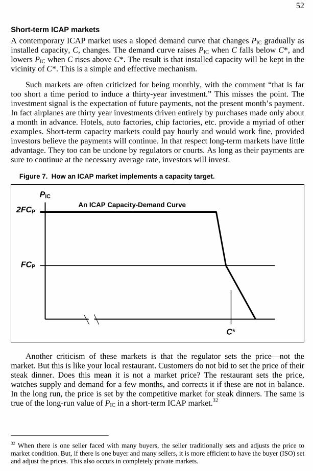
52

Short-term ICAP markets A contemporary ICAP market uses a sloped demand curve that changes PIC gradually as installed capacity, C, changes. The demand curve raises PIC when C falls below C*, and lowers PIC when C rises above C*. The result is that installed capacity will be kept in the vicinity of C*. This is a simple and effective mechanism.

Such markets are often criticized for being monthly, with the comment “that is far too short a time period to induce a thirty-year investment.” This misses the point. The investment signal is the expectation of future payments, not the present month’s payment. In fact airplanes are thirty year investments driven entirely by purchases made only about a month in advance. Hotels, auto factories, chip factories, etc. provide a myriad of other examples. Short-term capacity markets could pay hourly and would work fine, provided investors believe the payments will continue. In that respect long-term markets have little advantage. They too can be undone by regulators or courts. As long as their payments are sure to continue at the necessary average rate, investors will invest.

Another criticism of these markets is that the regulator sets the price—not the market. But this is like your local restaurant. Customers do not bid to set the price of their steak dinner. Does this mean it is not a market price? The restaurant sets the price, watches supply and demand for a few months, and corrects it if these are not in balance. In the long run, the price is set by the competitive market for steak dinners. The same is true of the long-run value of PIC in a short-term ICAP market.32

32 When there is one seller faced with many buyers, the seller traditionally sets and adjusts the price to market condition. But, if there is one buyer and many sellers, it is more efficient to have the buyer (ISO) set and adjust the prices. This also occurs in completely private markets.

2FCP

C*

PIC

Figure 7. How an ICAP market implements a capacity target.

An ICAP Capacity-Demand Curve

FCP

53

Forward ICAP markets A forward ICAP market (FCM), relies on new-entry to set the PIC. Consequently, a forward capacity auction typically purchases capacity three years in advance. New capacity contracts would typically have a duration of one to five years. Four years is suggested. Because load grows, the annual auctions typically buy 1% to 3% new capacity.

Theoretically the demand curve for the auction should reflect the marginal value of capacity, but a vertical demand curve will suffice for the Basic FCM Design. This vertical demand curve is administratively set at C*. When the auction is held, existing capacity will typically total less than C*, and since it is cheaper to supply existing capacity (usually almost free), new capacity will set the price.

Investors will observe the design of the FCM and see that it will take back the average scarcity revenue paid by the energy market, and that if they are Good suppliers—that provide their share on average during scarcity events—they will earn nothing from the performance incentive. Hence a Good Benchmark supplier will simply bid its fixed costs, FCP. A better than Good supplier will subtract off its expected performance bonus, while a poor supplier will bid above its fixed costs because it will ultimately earn less than the clearing price, PIC. A baseload unit will subtract its expected inframarginal rents from its fixed-costs when it bids.

It may seem that investors are forced to make complex calculations in order to bid correctly, but investors must always make such calculations when deciding to invest. They must always predict all of their future sources of income and all of their future costs. The FCM simplifies their predictions by making it easier to predict the future fluctuations in scarcity revenues. Under FCM these fluctuations will be fully hedged—they will be zero if their performance is Good. That is an easy prediction. Fixed cost recovery will no longer undergo wild swings because the market is short or long on capacity (even if it really is), or because the summer is hot or cold, or because a nuclear unit has gone out unexpectedly. All of these difficult-to-predict circumstances that now have dramatic impacts on profit will no longer matter. That will simplify the decision of whether to invest or not, and the decision of how much to bid. It will also reduce investor risk and the risk premiums passed on to consumers.

Investors will still need to predict future earning from the FCM, in other words future PIC levels. Providing new investors with a relatively long contract will assure investors that they will be paid at least their bid price during their first several years of operation. (Of course this will be somewhat adjusted by their performance bonus.)

Once a new supplier’s initial contract expires, it will start relying on the annually set PIC over which it has essentially no control (just as it has no control over energy prices). Because PIC provides a major source of fixed-cost recovery for all suppliers, it should be as stable and predictable as possible while still being determined by the market. To this end, PIC should be free of market power effects to the extent possible, and should not fall to zero if there are a few MW of excess capacity. This is accomplished by setting PIC on the basis of new-entry bids alone because it is existing capacity that has the most potential for exercising market power. On rare occasions, when no new entry is required

54

and as a consequence, there are too-few new-entry bids to competitively determine a price, PIC should be set a little lower than last year’s PIC, perhaps 10% lower.

Basic Design summary: 1) Estimate FCP and SR for a Benchmark unit and select C*. Set M = FCP / SR. 2) Hold an annual auction three years in advance to purchase C* capacity and

determine the clearing price, PIC. 3) Pay auction winners, PIC – SRShare + (M – 1) ( SR – SRShare ),

where SR is a supplier’s actual scarcity revenue, and SRShare is that supplier’s Share of capacity sold in the auction times total SR.

4) New entrants get four-year contracts, existing generators, one-year contracts. 5) Loads pay monthly FCM cost in proportion to their estimated annual peak load. 6) Zones are priced according to inter-zonal transmission limits and nodal-pricing

formulas.

55

12. Additions to the Basic Design The Basic short-term ICAP design is relatively complete, but the Basic FCM Design described above is intended only to illustrate the central ideas of FCM and is missing many important practical features. A number of these are discussed below, but no attempt will be made to present a complete working design, which should in any case be tailored to the particular market. The features discussed below are (1) market power in the FCM auction, (2) the descending clock auction, (3) the call options (4) capacity exports, (5) lumpy supply bids, (6) the definition of capacity, and finally (7) implementation.

1. Market Power in the FCM Auction All RA approaches require load to purchase something, mandatory hedges, obligatory call options, or in the case of FCM, capacity contracts. This requirement is actually a demand for a product imposed on load, and load’s demand simply reflects this regulatory obligation. Such obligations are generally quite inelastic. They say “buy this much,” rather than, “buy extra if it is cheaper and less if it costs more.” Long-term RA approaches have generally specified a vertical, completely inelastic, demand curve, and FCM is no exception. Unfortunately, inelastic demand is the classic way to give suppliers market power.

A forward auction combats market power by allowing new entry, but since the auction only buys 2% new capacity in any given year, one cannot depend on enough bids to supply 20% new capacity. No one wants to spend a lot of money planning an investment that has only a small chance of being realized. If the supply curve ends at, say, 8% new entry, then existing suppliers could withhold 6.1% and drive the clearing price to the auction’s starting price. In the ISO-NE design, this would double the clearing price received by the 94% of capacity not withheld. If existing capacity is allowed to withhold and drive up the price of contracts, all of the long-term approaches are in danger from the exercise of market power.

The purpose of FCM is to make sure that the market has enough installed capacity, not to induce installed capacity to sell energy. Hence, existing capacity is considered installed capacity, whether or not it chooses to bid in the FCM auction. It can only lose this status by retiring, exporting, or mothballing. To prevent withholding and market power, existing units are counted as supply in the FCM auction unless they request to retire, export or mothball. In these cases, certain restrictions, consistent with the nature of the request, and inhibiting of market power, can be placed on them.

2. The descending clock auction The auction should use a descending-clock design. This type of auction starts by naming a high opening price, 2×FCP, or roughly twice the eventual clearing price, is an appropriate choice. At that price, all suppliers must bid in all of their proposed supply. They cannot increase quantity as the price descends. At fixed intervals the auctioneer lowers the price and suppliers can reduce their quantity bids (they do not bid price). When the quantity becomes insufficient to meet the target capacity level, C*, the auction stops and the last price at which the target was met is selected as the clearing price, PIC.

56

There are three general techniques for structuring the auction to reduce market power. The first is to ignore existing suppliers who wish to withhold but do not wish to retire, export or mothball. Their capacity will remain installed capacity and it would be foolish to allow them to force load to buy new replacement capacity to replace capacity still in the energy market.

The second technique is to purchase only a limited amount of new capacity in the main auction and use the first of several reconfiguration auctions to top up new capacity as needed for special circumstances.33 The quantity of new capacity purchased in the main auction might be the greater of the years load growth and the amount needed to reach C* without considering retirements, exports and mothballs.34 This prevents existing supply from withholding from the main auction which sets the price of existing supply (90%+ of capacity), which greatly reduces its market power. The price of some new capacity could still be manipulated in the re-configuration auction, but such manipulations increase total installed capacity and reduce future auction prices.

The third technique is simply to require all export bids to be entered before the auction. In a descending clock auction, bids are quantities, but when entered before the auction, a price and quantity to be withdrawn are stated. The descending clock design allows bidders to learn more about the market as the auction proceeds, which results in more efficient bids. Such informational effects will not be dramatic, but the descending clock mechanism has many advantages and should be selected.

3. Call Options In order to allow all capacity, even old inefficient capacity to have a full physical hedge of their call option, it is best to raise the strike price of the call options to roughly three times VCP. This will also prevent the real-time market from being too risk-free and attracting too much participation relative to the DA market.35 It will also prevent gas price fluctuations from pushing VCP above the strike price. A higher strike price will require a higher multiplier, M, but no other changes.

4. Capacity Exports from CAISO Because export capabilities from CAISO are so extensive, exports of capacity pose a particularly severe threat of market power. Since the seasonal pattern of energy imports and exports is quite systematic it may be possible to simply forbid the exporting of capacity during certain seasons and thereby achieve sufficient protection from market power.

5. Lumpy Supply Bids Supply bids will generally specify quantities that correspond to units or a group of units that are cheaper when built as a group. Consequently it will not be possible to buy exactly the amount specified by the demand curve. Accepting partial bids would impose

33 It may be possible to, combine the first reconfiguration auction with the main auction. 34 If load growth is greater than the total required new capacity, only the total should be purchased. 35 To prevent too much weight from being placed on DA bidding requirements, suppliers should be allowed the use of virtual bids.

57

unnecessary risk on new suppliers and does not correspond with reality, so the auction will either accept an entire new-capacity bid, or none of it.

Export and import bids will be accepted in part when appropriate. If accepting the entire quantity for export would reduce C below C*, then only a fraction of the bid is accepted for export, the rest remains with the ISO.

6. Defining Capacity Suppliers bid a quantity of capacity, but they cannot be allowed to determine the capacity rating of their own units. Instead, a capacity bid should be either its nameplate value or something determined by the ISO’s engineers. The traditional EFORd value would be better than nameplate, but on wind units, this can be over 90% for a unit whose average performance is 30%. This is mainly a problem if too low a value for M is used, but this will likely be the case because it is difficult to estimate M accurately (as it comes from the energy-only design track) and suppliers will argue strongly for a low M to favor their existing plants.

To understand the problem, consider a half-strength performance incentive (M is half what it should be). Suppose the average PIC is $6/kW-month and a non-performing unit would lose on average only half of that. A 100 MW wind farm with a 40 MW average performance would lose half the difference between 100 and 40, and would be paid exactly as a perfectly performing 70 MW wind farm. It would be best if an engineering-base rating of 40 MW could be given to such a wind farm. Then it would perform on average as rated and be paid PIC for 40 MW with no correction due to performance incentives.

It would be best to start with an engineering-based estimate of capacity and then adjust it each year towards the previous year’s performance. For example, using a 20% adjustment rate, if the initial estimate were 40% and the performance was only 30% in the first year, then the second years value would be 38%.

7. Practicality of Implementation Centralization vs. bilateral contracting. The FCM is centralized exactly as a nodal energy market is centralized. As with a nodal market, centralization does not prevent every central-market transaction from being hedged with bilateral contracts. In fact, having a central market makes the bilateral markets more efficient and gives small participants the option of relying on the central market as a low-cost alternative.

Administrative parameters. Every solution to the RA problem depends on centrally set parameters. An FCM sets two key parameters, M, the scarcity revenue multiplier and C*, the installed capacity target.36 These determine respectively, the performance incentive and the market’s equilibrium level of installed capacity. The multiplier need not be accurately determined. Current ICAP markets have a multiplier of one, when it should be in the range of 3 to 9 because that is the extent of current energy-price suppression. Using an M of 3 when it should be 5 would still be excellent progress. 36 An energy-only market sets VOLL, in place of C*, and the energy-demand-curve parameters.

58

Auction complexity. Compared to holding a daily nodal-price auction that produces tens of thousands of prices per day, the FCM auction is child’s play. It produces one price per year per zone for the main auction and the same for each of perhaps four, much smaller, reconfiguration auctions. Preparing bids is the major effort, but the auction simplifies life for investors. The auction provides a far better signal of whether the project is worth doing than can be attained in a completely decentralized market. If you cannot beat your competitors in the auction, you can drop the project before you break ground. And if you do win, you get a guarantee of substantial fixed-cost coverage for the first four years of operation. Moreover the expected revenue from scarcity revenues is far more predictable with than without the FCM because these are hedged.

Load’s role. Load must pay its share of PIC when the ISO sends it a bill. It is best if load’s share can be adjusted monthly, and this will likely result in some complex accounting of customers. But this is entirely unnecessary. The LSEs’ monthly load is already tracked, and this can be used to accurately predict their peak annual loads. A little data and some spreadsheet statistics can do the job.

Monitoring Suppliers. The primary determinate of suppliers’ payments is simply their scarcity revenues in the existing and unaltered spot energy market. This is already tracked by the ISO’s accounting department. A more difficult task is estimating a unit’s effective capacity. For example, wind turbines typically have an effective capacity, as determined by their scarcity revenues, of roughly 30%. But this can be done once at the beginning according to the unit’s type and then adjusted annually based on SR / SRShare.

Zonal Parameters. If a zonal version of FCM is to be used, and this is recommended, each zone will need its own C*, and quantification of the transmission limits between zones.37 Again, these are values the system already needs to track for reliability purposes. The auction will need to determine different prices for each zone. The pricing principles are just marginal-cost pricing, the same as used for nodal pricing.

Contrary to the claims of some energy-only advocates, there is no need “to arrange

for transmission delivery or link the contract to any particular generating facility.” Bilateral contracts for ICAP are entirely financial, just like bilateral contracts for energy.

Summary of Implementation. A central FCM is more complex than a short-term ICAP with similarly hedged High-Spot-Prices because of the descending-clock auction and the yearly reconfiguration auctions. But by nodal pricing standards, it is simple. An FCM is basically like an extremely slow nodal pricing market with very few nodes.

37 The NYISO has defined C* for two zones, NYC and Long Island, and for the entire control area. This is logical from a reliability perspective, but requires a slight change in the nodal pricing formulas. It does not require a change from marginal-cost pricing, but simply its application with a “nested” approach as NYISO has done. N zones will always require N values of C* and will produce up to N distinct prices.

59

13. The Final Step to Convergence In October 2000, Harry Singh began his short paper on a call option alternative to ICAP with these observations.

There are at least two distinct approaches for ensuring generation adequacy… The first approach … involves setting Installed Capacity (ICAP) obligations…. An alternative approach relies primarily on spot price signals in the energy market.... A new approach is proposed that combines elements of both paradigms and relies on call options for energy. (Singh 2000, p. 1)

Singh’s proposal was five years ahead of his time and received little attention. Although his proposal did not address the missing money problem directly it pointed explicitly towards a convergent design. Five years later we have a workable new approach that combines these two elements. The energy-only and capacity-market tracks of resource adequacy design have nearly converged, with only one major discrepancy remaining. This convergence includes the following conclusions:

1) The source of the adequacy problem is the suppression of scarcity prices. 2) This results in missing money and missing performance incentives. 3) Both should be restored. 4) Restored high energy prices should be used for performance incentives. 5) High energy prices should be hedged with call-options.

This is a remarkable convergence, but it still leaves two questions unresolved. Because they are linked by design consideration, there is only one remaining fundamental choice.

The choice is between two design combinations: Design Combination 1: The capacity-target approach. Load is obligated to purchase C*

of hedged capacity exposed to High Spot Prices. Unpurchased capacity does not receive High Spot Prices.

Design Combination 2: The energy-price-control approach. All capacity receives High Spot Prices, and load is obligated to purchase C* of physically-backed hedges.

High Spot Prices are prices that are high enough to induce C* on their own. As can be seen, the differences between the two designs are so subtle that they seem almost not to matter. However, they do matter, because they change incentives substantially.

Supplier incentives. Under the capacity-target approach, suppliers who do not sell their capacity along with a hedge do not receive high prices and consequently do not have their missing money restored. This means they lose, in our Standard Example, $60,000/MW-year. Under the energy-price-control approach, suppliers who do not sell a physical hedge, still receive High Spot Prices and consequently experience only an increase in risk. They have no expected (average) loss of revenue. While risk reduction has value, risk premiums are only on the order of 10%, so the motivation of suppliers to participate in hedging is roughly ten times greater under the capacity-target approach.

60

Load incentives. The motivation for load to participate in hedging is also quite different under the two designs. Under the capacity-target approach they must purchase hedges. Under the energy-price-control approach, load simply faces greater risk from higher spot prices if they do not. Since load purchases almost no forward contracts in the three to seven year range with a $1000 cap, it is unlikely that they will opt for full coverage simply because the cap is raised to $5000. The sources of the dichotomy. The capacity-target approach corresponds to ISO-NE’s LICAP design and the FCM design presented here. The energy-price-control approach corresponds to Hogan’s design in which first prices would be raised for the entire market, and second, mandatory hedges would be imposed on load.

Implications for Investment stability To see how the two Design Combinations differ with respect to investment incentives, consider a case where the High Spot Prices are actually set twice as high as needed. Design Combination 1: The performance incentive will double. The investment level will

be unaffected. Design Combination 2: The fixed cost recovery of peakers will double at C*. This will

push C well past C*. Performance incentives will also double. On the other hand, if High Spot Prices were set half as high as needed the result would not necessarily be symmetrical but opposite. Design Combination 1: The performance incentive will halve. The investment level will

be unaffected. Design Combination 2: Assuming load’s obligation to purchase C* of hedged capacity is

backed by sufficient penalties, this obligation would take over and hold installed capacity to C*. The purchase price will be inflated by market power. Performance incentives will halve.

Design Combination 2, the energy-price-control approach, uses belts and suspenders. Whichever sets the higher standard, C* or the High Spot Prices, will dominate, unless the capacity requirement is weak-kneed. In fact energy-only approaches spend almost no time describing load’s obligation or its enforcement, and their rhetoric indicates they intend to rely on load aversion to risk as the main inducement to buy hedges. So their enforcement of the mandate or obligation may be intentionally weak. So far, except for Singh’s combined approach, there is no sign that energy-only approaches would use the mandate or obligation to drive up the price of hedges to replace missing money and induce investment. If they do not, then they rely entirely on the erratic method of spot-price control.

Because the capacity-target approach is a more accurate method of inducing the desired level of reliability, it seems inappropriate to add on an erratic energy-price method of controlling investment. Better to let the capacity-target handle the adequacy problem and let the hedged spot prices handle the performance incentive, risk management, and market power problems. Each design track should do what it is good at and what it was intended for.

61

Implications for Market power Under Design Combination 1, if a supplier withholds capacity from the physical-hedge market, it loses not just the hedge, but the High Spot Prices. This makes withholding quite expensive. Nonetheless, the auction design for ISO-NE’s long-term capacity market is largely focused on preventing existing generation from exercising market power. If withholding were practically free, the problem would be much more difficult. Design Combination 2 would make withholding much cheaper. But another consideration further aggravates the market-power problem of Design Combination 2.

As just discussed, it is difficult to define the exact role of the hedge obligation specified in energy-only designs. It appears that load is to be largely motivated by a desire to avoid risk and market power, and that the obligation is intended to play only a minor role in motivating load’s purchase of the obligatory hedges. The idea is that load has almost enough economic motivation and just needs a small push from the regulator.

An “energy-only” market design could accommodate a mandatory load hedge (MLH) requirement. This would be a regulatory intervention to address the concern that there would be inadequate forward contracting. (Hogan 2005, p. 27)

This means some penalty for non-compliance is needed and both Oren and Bidwell mention such penalties. But the idea of a “regulatory intervention to address the concern that there would be inadequate forward contracting” has been previously addressed by Hogan and Harvey (2000) in “California Electricity Prices and Forward Market Hedging,” published in the midst of the California meltdown.

This paper argues against the position of the CAISO’s Market Surveillance Committee (MSC), which stated in its September 2000 report that “Eliminating restrictions on UDC [LSE] forward financial contracting can significantly limit the ability of generators to exercise market power.”38 The idea of that report was that if LSEs could hedge, they would sign forward contracts with suppliers and this would essentially eliminate the market power of the suppliers.

But Hogan and Harvey argue that while long-term contracts certainly reduce spot market power, suppliers will demand a high price for signing contracts that eliminate their market power, and that was when the CAISO’s price cap was $250, not the $10,000 level now proposed.

Relying on buyers to engage in forward market hedging per se is not likely to have significant benefits in mitigating the market power of sellers. (p. 1)

We find that there is little or no evidence to support the argument that the mere opportunity to arrange long-term forward market contracts would mitigate market power. … placing the pressure on the buyers in the current market might have the opposite of the intended effect, leading to higher not lower overall costs. (p. 2)

38 UDC or utility distribution company is equivalent in this context to today’s load serving entity (LSE).

62

The common sense question looms as to exactly why generators possessing market power would be prepared to offer low price contracts in order to lower the spot price and lower their own profits? (p. 7)

On balance, therefore, the net implication of these various game theoretic formulations is at best mixed, and there is no compelling theoretical argument that would support the conclusion that generators possessing market power would unwittingly surrender that market power simply because customers came asking for long-term contracts. (Harvey and Hogan 2000, p. 8)

To summarize, under Design Combination 2, the regulator will have to apply considerable pressure on the buyers to get them to pay enough so that suppliers surrender that market power which they have gained from the new $10,000 spot prices. Although arguing against the implications of a cheap transition to long-term contracting implicit in the MSC report, Hogan and Harvey point out that to some extent the MSC actually agreed with their analysis.

In making their forward contracting decisions, load-serving entities must trade off the benefits of reduced average spot prices against the increased prices that they may need to be pay in forward markets to purchase a sufficient amount of forward energy to cause generators to bid aggressively in the spot energy markets.

Generators must bear in mind that signing significant long-term financial forward commitments to supply energy, even at very attractive prices, commits them to be very aggressive suppliers of energy in the spot market, which can reduce average spot prices. –MSC Report, p.10.

It appears the two sides were not far apart, and both agreed that LSEs would need to pay increased prices to induce suppliers to give up their spot market power. What can be done about this dilemma? Now that spot prices have been suppressed and we are contemplating restoring them to a more appropriate level, there is a simple answer. Do not give the suppliers the High Spot Prices and then Mandate that load pay increased prices for forward contracts to buy back the market power just handed to the suppliers with the $10,000 price cap. Instead, use the High Spot Prices as a carrot for the generators. Offer them high prices if they sell the load a hedge—if they surrender their market power in advance.

It would be possible for load to take advantage of existing suppliers by keeping their prices suppressed while purchasing new generation with RFPs. That is not the suggestion; this is simply to note how much power load now has. Load can easily use that same power to ask suppliers to give up their spot market power before they are given High Spot Prices. This is what Design Combination 1 does.

63

14. Conclusion Energy markets were quite efficiently dispatched under regulation and improved dispatch was not a primary reason for restructuring. Better investment and performance were primary reasons and some striking improvements have been seen in the performance of nuclear units, among others. But investment has been more subject to boom-bust cycles and risk premiums have increased from among the lowest of any industry to among the highest. Both effects can impose significant cost on consumers.

To achieve the central objectives of restructuring, three problems must be addressed. (1) Generating resources must be stabilized at an adequate level (the quantity problem). (2) Investors must efficiently tradeoff costs against plant characteristics, such as flexibility, needed by the system (the quality problem). (3) Existing plants should be operated and maintained efficiently in keeping with unsuppressed real-time prices (the performance problem). The root of all three problems is the same—price suppression for the sake of controlling market power.

Although a Resource Adequacy program is focused on the first problem (quantity), solving this may only restore the stability lost in the move to competition. To capture the promise of restructuring, the second two problems must also be solved. Because all three have the same root cause, it is sensible and efficient to solve all three at once. Naturally, such a design starts by restoring the High Spot Prices that have been suppressed. This requires (1) that load be protected from the negative market power and risk side effects of high prices. Consequently, (2) load must be fully hedged. Call options can do this without interfering with the performance and quality incentives of high prices. The price paid for these call options will control the level of installed capacity, so (3) call option prices are determined in an annual forward auction for new capacity.

Such a program is the most market-based solution currently possible. It relies on the market to solve both the quality and performance problems. It also relies on the market to determine the cost of new capacity. It is not yet possible for the market to determine what quantity of capacity is required to satisfy the consumer’s desire for reliability, because this desire is not expressed in current markets.

A stable capacity market would assure adequate reliability, prevent crises caused by underinvestment, reduce market power in the energy market, and perhaps most significantly, greatly reduce the industry’s risk premium which otherwise promises to raise the cost of all existing capacity through the law of one price.

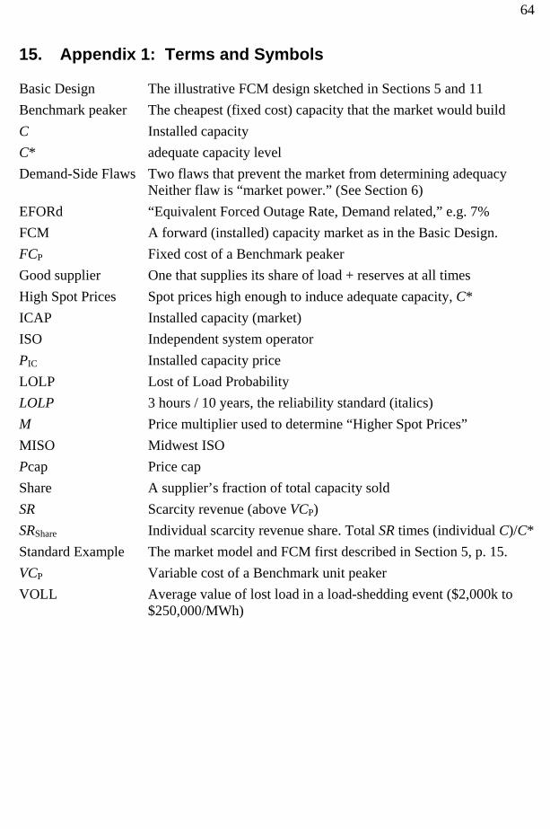
64

15. Appendix 1: Terms and Symbols Basic Design The illustrative FCM design sketched in Sections 5 and 11 Benchmark peaker The cheapest (fixed cost) capacity that the market would build C Installed capacity C* adequate capacity level Demand-Side Flaws Two flaws that prevent the market from determining adequacy Neither flaw is “market power.” (See Section 6) EFORd “Equivalent Forced Outage Rate, Demand related,” e.g. 7% FCM A forward (installed) capacity market as in the Basic Design. FCP Fixed cost of a Benchmark peaker Good supplier One that supplies its share of load + reserves at all times High Spot Prices Spot prices high enough to induce adequate capacity, C* ICAP Installed capacity (market) ISO Independent system operator PIC Installed capacity price LOLP Lost of Load Probability LOLP 3 hours / 10 years, the reliability standard (italics) M Price multiplier used to determine “Higher Spot Prices” MISO Midwest ISO Pcap Price cap Share A supplier’s fraction of total capacity sold SR Scarcity revenue (above VCP) SRShare Individual scarcity revenue share. Total SR times (individual C)/C* Standard Example The market model and FCM first described in Section 5, p. 15. VCP Variable cost of a Benchmark unit peaker VOLL Average value of lost load in a load-shedding event ($2,000k to

$250,000/MWh)

65

16. Appendix 2: Frequently Asked Questions 1. Why is a “peaker” the right standard for missing money? 2. Why is VOLL relevant? 3. What if parameters are estimated too high? Will consumers overpay? 4. Isn’t there something wrong with such high ICAP prices? 5. Doesn’t Australia’s market prove the energy-only approach works? 6. If markets have no clue as to reliability, why do they work at all? 7. Don’t we have too much reliability and isn’t this very expensive? 8. How much demand elasticity do we need before the market can take over? 9. Are risk premiums important compared to the capacity level ? 10. What are the main differences between ISO-NE’s LICAP and FCM?

1. Why is a “peaker” the right standard for missing money? Any type of unit could be used as the benchmark unit, as they all give the same answer to the question how much scarcity revenue is needed. Consider a market with two types of units, baseload and peaker. In equilibrium, both units will cover their fixed costs, but if scarcity revenues are defined as revenues accruing from the part of price that is above the highest variable cost, VCP (the variable cost of a peaker), then baseload units cover fixed costs with a combination of infra-marginal revenues (from the part of price below VCP) and scarcity rents, while peakers can only cover them with scarcity rents. Hence we know a peaker must receive scarcity revenue = FCP to break even.

In equilibrium, baseload plants must also break even, and they should earn the same amount of scarcity revenue as a peaker since they are just as likely to be running when price is greater than VCP as is a peaker. They cannot be earning either too much or too little in equilibrium, otherwise it would not be an equilibrium. Hence, in equilibrium, a baseload plant needs to earn FCP of scarcity revenue in order to break even. In fact, this is the scarcity revenue needed by any type of plant to break even when the market is in equilibrium with the optimal mix of plants.

2. Why is VOLL relevant? When supply can equal demand, economics tells us that price should be set to make them equal. If neither side is exercising market power (trying to influence the market price), the price that brings about this equality is the competitive price. This tells us how to set price at all times when supply can equal demand. But when this is impossible what should be done? Supply cannot equal demand at times when demand is greater than the amount of supply physically available, and in this case, some load will be shed. The question then becomes what should be paid when there is load shedding, or as it is sometimes call “lost load.”

The market cannot answer this question because markets cannot set an efficient price when the supply and demand curves do not intersect. But there is an answer. There is a price that, like a competitive price, is efficient because it makes consumers and suppliers do the right thing to greatest extent that any price can, given the infrastructure. There is a price, which if set whenever load must be shed, will lead to the optimal level of

66

investment. This is the price that maximizes total consumer benefit minus the cost of production including both marginal and fixed costs.

The efficient price when load must be shed is VOLL, the value of lost load. In fact, the VOLL is best defined as the price that will neither overbuild nor underbuild capacity if it is paid whenever load is shed. Defined that way, it can be shown to equal (for simple models of consumer utility) the average value (willingness to pay) of serving one more MW of load rather than shedding it.

Although it is very difficult to determine this value, it is still an important value because it is the value that indicates how much reliability consumers are willing to pay for and how much capacity should be built. Any other value reflects the engineers or regulators desires, rather than the consumer’s valuation.

3. What if parameters are estimated too high? Will consumers overpay? In a short-term ICAP market, the demand curve is set to pay the estimated annualized cost of a new Benchmark peaker, about $95,000/MW-year in ISO-NE. If this turned out to be high by $35,000, which is about the most imagined, the market will balance with about 3% too many peakers (assuming the LICAP demand curve). With this much extra capacity, the ICAP demand curve will set a price of $60,000.

In New England, where there is excess capacity, the price would start even lower, and the capacity level would fall until it stopped at 3% above the target, and there would be no overpayment. Once this happens the demand curve would be lowered to reflect re-estimated peaker costs. Three percent extra capacity increases retail costs by about one half percent and this would only last till the curve was adjusted. In a forward capacity market, the capacity price is based on new entry bids, so it is not affected by any error in estimating FCP.

The multiplier, M, only affects performance, not average cost. With M too high suppliers will perform slightly better than consumers would want to pay for, but the resulting inefficiency would be small unless M was drastically over estimated.

4. Isn’t there something wrong with such high ICAP prices? Currently U.S. electricity markets are in an unfortunate position. Gas prices have more than doubled; gas prices frequently set the market price, and baseload units are reaping windfall gains. This is one of the un-advertised risks of using markets. So far, this cost impact has been disguised by a surplus of capacity which depresses energy prices. However, when new capacity is needed, a market approach requires that ICAP or energy prices paid to every unit must increase to the point where investments will at least break even. If we are lucky, non-gas baseload plants will enter at low ICAP prices, because they are currently so profitable. But if there are barriers to baseload entry, the ICAP/energy price may need to rise to cover the cost of a benchmark peaker.

The result could be energy costs that are considerably higher than under regulation, because regulation does not permit sustained windfall gains from changes in relative fuel prices. The data indicate that this may become a problem in ISO-NE. A market will permit such gains until the technology mix can readjust.

67

5. Doesn’t Australia’s market prove the energy-only approach works? We asked an independent investor with experience in three different international markets to gives us his opinion of Australia’s market. This is his reply.

“My view of the Australian market was that the veneer of privatization was pretty thin (about 2/3 of the generation is publicly owned and more than ½ of the retail), that retail competition was not particularly effective, and that investment decisions were often influenced by government policy rather than purely market forces. During my stay there, pool prices hovered in the $25-$35 range. The energy component of retailers’ bills were >$60. I’d have guessed that the cost of new entry for baseload plant would have been >$45 (gas) and >$50 (coal).

I’ve asked the guys in our Australian office to compile a list of the generation adds during that period, but my recollection was that even in the face of pool prices that apparently were below the cost of new entry, significant entry nonetheless occurred (both coal and gas). Some of the gulf in the economics would be attributable to environmental legislation which was coming into effect and was structured as an incentive for new. It was my guess however, that much was also the result of other government policies (particularly in Qld) which saw government owned generators contracting with government owned retailers at out-of-market prices to underpin the new plants.

It’s hard to know what the deals were but I’d suggest that before anyone placed too much faith on the Australian model, they at least check into the possibility that non-market forces may be playing a significant role.”

Oren (2005) appears to agree: “all the designs … worldwide abandoned the principle that ‘the market should determine the desirable level of investment’ and are relying on engineering based determinations of generation adequacy requirements. This is done … through publication of a long term statement of investment opportunity, like in Australia.”

6. If markets have no clue as to reliability, why do they work at all? Dynamic systems need stabilizers (negative feedback loops) to keep from wandering far from equilibrium. Capacity markets have gotten a few percent too tight, and have been overbuilt by ten or twenty percent, but that’s as far astray as they have wandered. This indicates there are stabilizers. What are they? First, regulators have set the energy-only parameters just about right. Energy prices may be four times too low, but they rise very quickly once capacity is in short supply. So even with this crude setting, we would expect the market to stay about in the range observed. Second, as was seen in California, if the market wanders a bit too far, a strong political feedback loop will activate and adjust the capacity level. Third, eastern markets include ICAP markets and these help keep the capacity level near the engineering target level. In other words, energy markets have at least three crude resource-adequacy mechanisms already in effect, and all three are controlled by administrators or politics.

68

7. Don’t we have too much reliability and isn’t this very expensive? We may well be buying more installed capacity than can be justified on the basis of increased reliability, but if so, it is costing us very little.

The word on the street, perhaps apocryphal, is that the one-day-in-ten-years standard was invented by two engineers who wanted to help their company sell more generators. Certainly, the standard could not look more suspicious. Where did the “10” come from? That is simply the roundest number, the base of our number system, and was probably determined by the fact that we have ten digits on our two hands. A year is the time it takes the earth to circle the sun. Could it be that these two facts exactly correspond with the amount of reliability consumers want, regardless of the cost of new generation?

This justified suspicion of gold-plated reliability has led economists to claim that we have a big problem, and are wasting a lot of money. Unlike engineers, economists frequently forget to use the backs of envelopes. Engineers have a pretty good feel for what is needed to run a power system. Certainly they like to have an easy time in the control room and may exaggerate system requirements for that reason. But there is overwhelming evidence that if the normal target of 118% of expected peak load were cut to say 108%, the engineers would be genuinely petrified, and the resulting rolling blackouts would cause headlines and political repercussions that would soon force a more conservative approach.

How much would this 8.5% reduction of capacity save? Extra capacity for reliability is the cheapest capacity to build because it is almost never used. The cost used in this paper is $80,000/MW-year, so saving 8.5% of 50,000 MW would save $340 million per year. If system load averages 25,000 MW and retail cost averages $120/MWh, total annual retail cost is $26.3 billion. Even if we cut reliability to the point where dispatchers were distraught, blackouts from inadequate capacity were commonplace, and power markets were in a constant meltdown, we would save consumers only 1.3% of retail costs ($340M / 26.3B).

This point is important because the desire to save on capacity by “letting the market decide” on reliability is the major driving force behind the energy-only VOLL approach to resource adequacy. Not only is the argument erroneous because the market has no clue as to the value of VOLL (so administrators will still drive investment), but the hoped-for savings is diminutive at best, and perhaps nonexistent.

8. How much demand elasticity do we need before the market can take over? We do not know. If we knew VOLL, and followed simple economic theory, this is how demand elasticity would eventually replace the regulator. First, economic theory says to set the real time price to VOLL only during load-shedding events. As demand elasticity increases below VOLL, suppliers will earn more scarcity revenue from prices set by demand. This means they will earn less from VOLL, which means there will be fewer load shedding hours, which means reliability will increase.

Contrary to the energy-only view, a well functioning market will likely buy more reliability, not less. As load shedding due to adequacy problems becomes less frequent the value of VOLL will play a smaller roll. Eventually VOLL = $2,000 and VOLL =

69

$250,000 will provide almost that same level of reliability because fixed cost recovery has shifted from 100% based on load shedding to 99% based on prices set by demand. At this point there is essentially perfect reliability with regard to adequacy problems (but not with regard to ice storms, lightning, nuclear outages, and other contingencies). One challenge in assessing this outcome is that the only legitimate demand elasticity comes from the part of the demand curve below VOLL, and we do not know VOLL.

9. Are risk premiums important compared to the capacity level ? A stable forward capacity market with solid backing from the CAISO and regulators, could quite possibly reduce risk premiums by 4%. In California, perhaps by 6%. The principle component of fixed costs is the required return on capital, about 15%. Suppose total fixed costs are 20% of the overnight cost, including the risk premium. Suppose a 5% risk premium was removed by a stable capacity market, dropping fixed costs to 15% of the overnight cost. This would reduce the fixed cost of a peaker from $80,000/MW-year to $60,000/MWh. Since the fixed cost of a peaker dictates the equilibrium price of all capacity (above inframarginal rents), this reduction would save $1 billion per year in a 50,000 MW system.

10. What are the main differences between ISO-NE’s LICAP and FCM? First note that FCM is not the approach being negotiated by the interested parties in early 2006. The negotiated approach contains some of the FCM design, but as is typical of ICAP approaches, stakeholders are adding many non-market-based features, particularly in the area of performance incentives. The main difference between LICAP and FCM is the use of a forward market to allow new capacity to set the price paid to all capacity. This should stabilize the level of installed capacity and stabilize the capacity price more.

The form of the performance incentive has also been changed, but this is more a matter of appearance than substance. LICAP charged suppliers roughly 1/N years worth of ICAP payment per shortage hour missed, where N is the number of shortage hours per year. If a supplier missed 20% of the shortage hours in one year, it would miss about 20% of LICAP payments for one year. Since the LICAP payment is equivalent to High Spot Prices, this incentive is equivalent to High Spot Prices. One difference from spot price incentives is that the shortage-hour penalty depends on how quickly new shortage hours occur. In spite of this, the shortage hour incentive does not depend on what comes after the missed hour, because this information is not known at the time of the shortage hour.

Like FCM, LICAP completely hedges load. Scarcity revenues above a certain strike price are subtracted from the LICAP payment. Hence, if there is a hot summer, with triple the normal amount scarcity revenue, this is subtracted from the LICAP payment and the combination of LICAP payment plus scarcity revenue does not change. LICAP payments can be viewed as purchasing a call option on scarcity revenues, exactly as proposed by Oren who criticizes LICAP without recognizing this similarity.

70

17. References Bidwell, Miles. 2005. “Reliability Options,” Electricity Journal, 18, June, 11-25.

Bidwell, Miles and Alex Henney. 2004. “Will the New Electricity Trading Arrangements Ensure Generation Adequacy,” Electricity Journal, 17, August/September.

Bushnell, James. 2005. “Electricity Resource Adequacy: Matching Policies and Goals,” CSEM WP 146, August.

California Public Utilities Commission. 2005. “Capacity Markets White Paper,” CPUC Energy Division, Sean Gallagher, Director August 25.

Chao, Hung-Po and Robert Wilson. 2004. “Resource Adequacy and Market Power Mitigation via Option Contracts,” Electric Power Research Institute, Draft, March.

Cramton, Peter and Steven Stoft. 2005. “A Capacity Market that Makes Sense,” Electricity Journal, 18, September, 43-54.

Hobbs, Benjamin F. 2005. “Affidavit of Benjamin F. Hobbs.” Concerning PJM’s new Reliability Pricing Model (RPM). Filed with FERC August 31.

Hogan, William W. 2005. “On an ‘Energy-Only’ Electricity Market Design for Resource Adequacy,” paper prepared for the California ISO, September 23.

Hogan, William W. and Scott M. Harvey. 2000. “California Electricity Prices and Forward Market Hedging,” October 17.

Jevons, W. Stanley. 1879. The Theory of Political Economy.

Joskow, Paul. 2005. “Why Capacity Obligations and Capacity Markets?” Slides presented at "The Economics of Electricity Markets," June, Toulouse, France.

Joskow, Paul. 2006. “Markets for Power in the United States: An Interim Assessment,” The Energy Journal, forthcoming.

Joskow, Paul and Jean Tirole. 2006. “Reliability and competitive electricity markets,” Rand Journal of Economics, forthcoming.

Midwest Independent System Operator. 2005. “An Energy-Only Market For Resource Adequacy In The Midwest ISO Region,” November 23.

NERA Economic Consulting. 2003. “Central Resource Adequacy Markets for PJM, NY-ISO and NE-ISO, Final Report, February.

Oren, Shmuel. 2005. “Generation Adequacy via Call Options Obligations: Safe Passage to the Promised Land,” Electricity Journal, 18, November.

Singh, Harry. 2000. “Call Options for Energy: A Market Based Alternative to ICAP,” PG&E National Energy Group, October.

Stoft, Steven. 2002. Power System Economics, IEEE Press.

Stoft, Steven. 2004. Testimony on Behalf of ISO New England on Locational Installed Capacity Market Proposal, Submitted to Federal Energy Regulatory Commission, Docket Number ER03-563-030; Direct August 31.

71

Stoft, Steven. 2005. “Testimony on Behalf of ISO New England on Locational Installed Capacity Market Proposal,” Docket Number ER03-563-030; Rebuttal February 10.

Wolak, Frank. 2004. “What’s Wrong with Capacity Markets?” June 23.