cranslik v1.0: stochastic prediction of oil spill transport and fate

Discussion

Pa

per|

Discussion

Pa

per|

Discussion

Paper

|D

iscussionP

aper|

Geosci. Model Dev. Discuss., 6, 7047–7076, 2013www.geosci-model-dev-discuss.net/6/7047/2013/doi:10.5194/gmdd-6-7047-2013© Author(s) 2013. CC Attribution 3.0 License.

Open A

ccess

GeoscientificModel Development

Discussions

This discussion paper is/has been under review for the journal Geoscientific ModelDevelopment (GMD). Please refer to the corresponding final paper in GMD if available.

CranSLIK v1.0: stochastic prediction ofoil spill transport and fate usingapproximation methodsB. J. Snow1,*, I. Moulitsas1, A. J. Kolios1, and M. De Dominicis2

1Cranfield University, Cranfield, UK2Istituto Nazionale di Geofisica e Vulcanologia, Sezione di Bologna, Italy*now at: Northumbria University, Newcastle, UK

Received: 11 October 2013 – Accepted: 12 December 2013 – Published: 20 December 2013

Correspondence to: I. Moulitsas ([email protected])

Published by Copernicus Publications on behalf of the European Geosciences Union.

7047

Discussion

Paper

|D

iscussionP

aper|

Discussion

Paper

|D

iscussionP

aper|

Abstract

This paper investigates the development of a model, called CranSLIK, to predict thetransport and transformations of a point mass oil spill via a stochastic approach. Ini-tially the various effects that affect the destination are considered and key parametersare chosen which are expected to dominate the displacement. The variables consid-5

ered are: wind velocity, surface water velocity, spill size, and spill age. For a point massoil spill, it is found that the centre of mass can be determined by the wind and currentdata only, and the spill size and age can then be used to reconstruct the surface ofthe spill. These variables are sampled and simulations are performed using an open-source Lagrangian approach-based code, MEDSLIK II. Regression modelling is ap-10

plied to create two sets of polynomials: one for the centre of mass, and one for the spillsize. A minimum of approximately 80 % of the oil is captured for the Algeria scenario.Finally, Monte-Carlo simulation is implemented to allow for consideration of most likelydestination for the oil spill, when the distributions for the oceanographic conditions areknown.15

1 Introduction

Whilst the frequency of spills occurring has dropped significantly in the last fewdecades, Etkin (2001), it does not diminish the inevitability of an oil spill occurring.Oil spills can cause large scale destruction of the environment, they have significanteconomical effects, and can result in human lives losses. They are inevitably the cause20

of environmental, economic, and human disaster. The Deepwater Horizon spill, for ex-ample, has been analysed extensively by Graham et al. (2011), members of the USNational Commission on the BP Deepwater Horizon Oil Spill and Offshore Drilling.There is therefore much interest in being able to accurately predict the destination,transport, and transformation of an oil spill to minimise the resultant cost, both financial25

and environmental.

7048

Discussion

Pa

per|

Discussion

Pa

per|

Discussion

Paper

|D

iscussionP

aper|

There are many complex phenomena affecting an oil spill, creating an advection–diffusion–transformation process. These consist of a large number of effects: the ad-vection due to currents, wind and waves, the diffusion due to the turbulence andthe transformation processes, such as evaporation, natural dispersion, spreading etc.,which need to be considered for accurate fate and transport prediction. There are nu-5

merous equations available which are created to model these effects, based on bothanalytical and empirical approaches, however the complexity of the underlying physicsis not yet fully understood. Reed et al. (1999) provide a very good summary of earlymodels. Since then significant progress has been made in acquiring a deeper under-standing of the involved complex phenomena, for example biodegredation is studied10

by McGenity et al. (2012).Difficulty also arises from the side of uncertainty since exact quantities are not neces-

sarily known beforehand due to the stochastic nature of certain variables, for examplethe sea surface velocity. The computational cost involved in running multiple cases,or Monte-Carlo simulation, to consider the possible conditions is often far too great to15

be a viable approach. This becomes a severe impediment in cases of real accidentswhere a quick, or even real time, prediction becomes necessary.

Many models have been developed and used to predict the transport and transforma-tion of an oil spill. These are either commercial, such as Li et al. (2013), or open-source,such as De Dominicis et al. (2013a). Regardless of the software tools employed, these20

models are not without their limitations. Often the computational cost involved in run-ning a full simulation is too high. Alternatively, in order to be able to have a predictionin near real time, the model has to be simplified extensively, in terms of its physics, andtherefore the simulation results are not of high accuracy.

This paper investigates the use of stochastic methods to map the response from dif-25

ferent input variables to create a robust and efficient software tool capable of effectiveprediction. This provides an estimation of the destination and spread of an oil spill sub-ject to oceanographic conditions. Also, due to the minimal computational time requiredfor the developed model, probable regions for the oil spill can be developed in real time

7049

Discussion

Paper

|D

iscussionP

aper|

Discussion

Paper

|D

iscussionP

aper|

via Monte-Carlo simulation. This aids significantly in reducing the resultant financialand environmental cost of oil spills, predicting their likely development.

The key steps in developing our methodology can be outlined as follows:

1. identify the key parameters and their relative distributions necessary for short termoil spill prediction.5

2. Apply sampling to the considered parameters to create a design hypercube.

3. Generate simulation data using the design hypercube.

4. Fit regression models to map the inputs to the response.

5. Use aforementioned regression model to create a prediction code.

6. Test the developed code against a real scenario and analyse the results.10

In order to generate simulation data, we have used the MEDSLIK II model. This choicewas based on a number of reasons, but predominantly due to its robustness and be-cause it has been validated on multiple real spills as discussed in De Dominicis et al.(2013b, a).

2 Physics and mechanics of oil spills15

As stated in the introduction, one of the main complexities of modelling an oil spill is ac-curately accounting for the many complex physical phenomena that are the advection–diffusion–transformation processes. As the water and oil interact, there are severalphysical and chemical reactions which occur and increase the complexity of the resul-tant flow physics. Reed et al. (1999) provide a summary of the state of the art models20

available at the time of publishing. However, significant advances have been madesince then, for example, the role of microorganisms in biodegredation is now betterunderstood as discussed in McGenity et al. (2012). In particular, Reed et al. (1999)

7050

Discussion

Pa

per|

Discussion

Pa

per|

Discussion

Paper

|D

iscussionP

aper|

provide an in depth analysis into the transport and weathering procedures and thevarying models used to account for complex flow behaviour. A diagram showing theseeffects can be seen in Fig. 1 (MEDESS-4MS, 2013; ITOPF, 2013).

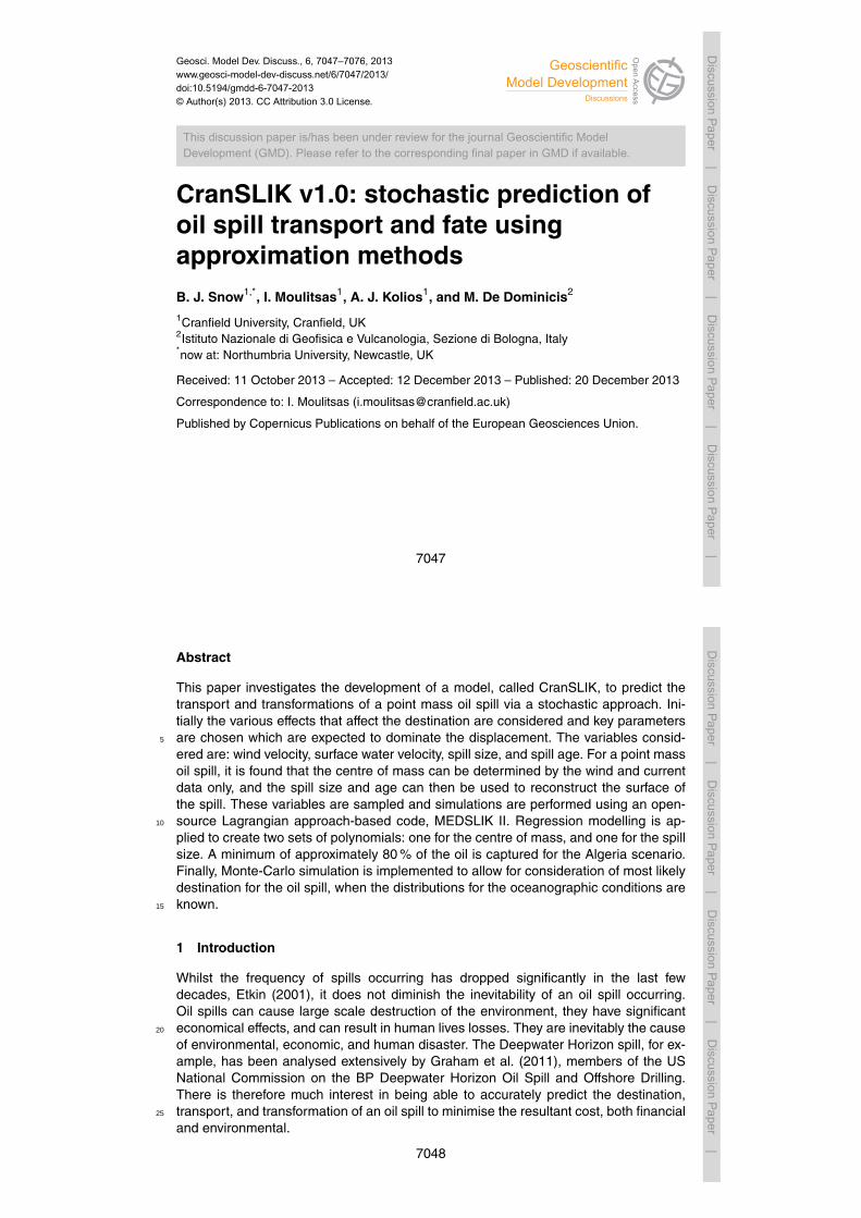
The importance of these effects varies over time and a speculative mass balancecan be seen in Fig. 2 (Mackay and McAuliffe, 1989). This implies that, for short term5

modelling, it is not necessary to fully resolve all phenomena. However, different con-siderations will need to be made in order to provide accurate predictions over longerperiods of time.

2.1 Advection and turbulent diffusion

Advection is a three dimensional process whereby the oil is transported due to wind,10

wave and current forcing. Traditionally this was thought to be a two dimensional effecthowever there have been numerous demonstrations of the importance of the verticaloil motion, including experimental (both field and laboratory) and computational simu-lation studies. Determining the magnitude of these effects is difficult due to the complexphenomenon that causes them.15

The most important factor in the advection process is the current forcing. This isresponsible for the majority of the displacement due to the direct contact between thewater and the oil. The oil can also be transported vertically into the water column bythe current and hence both the horizontal and vertical current shear are important inthe motion of an oil spill (Reed et al., 1999).20

Wind speed can be separated into two main components: long term and shortterm. The short term fluctuations are traditionally modelled by a Weibull distribution(de Prada Gil et al., 2012). Results have shown though that this may be a rather poordistribution. In Morgan et al. (2011) other possible distributions have been investigatedand the produced results suggest that the 2-parameter Log-normal model is most ap-25

propriate for extreme wind speeds however still possesses significant errors. The windspeed also varies greatly upon the position on the globe one is interested in.

7051

Discussion

Paper

|D

iscussionP

aper|

Discussion

Paper

|D

iscussionP

aper|

A similar problem exists for prediction of wave propagation. There is the generationof turbulent kinetic energy from the breaking of waves. Fay (1971) suggests that the firstorder effects of surface waves are negligible due to their periodic nature. The wavesproduce oscillatory forces which have a mean velocity component of zero. Therefore,over a sufficiently long time scale, the first order waves are negligible. Fay (1971) does5

however make note of the existence of non-linear waves which can affect the spreadof oil.

2.2 Spreading

Another effect is the spreading of the oil due to film thickness and area. The classicequations to estimate the spread of an oil were defined by Fay (1971) and can be seen10

in Table 1. By making the assumption of no wind, wave or current effects, he suggesteddifferent spreading laws for both one-dimensional and axisymetric flows. The assump-tions are justified in terms of importance, assuming that these effects are superimposedon the spreading motion. However, it is stated that without consideration of wind andwave effects, there is very little practical application for these equations. To derive his15

equations, the various effects that might enhance or inhibit spreading are considered:gravity, inertia, surface tension, and friction. Whilst gravity acts in the vertical direction,there is a horizontal effect on the oil and an uneven pressure distribution is created.This forces the oil to spread out into an increasingly thin film over the surface of thewater. The surface tension also plays a role in this expansion and eventually becomes20

the main driving force. The rate of spread is restricted by the inertia and the friction.The effect of inertia decreases as the film becomes thinner. The friction is due to thesmall amount of water underneath the film.

2.3 Evaporation and emulsification

Evaporation is one of the key oil transformation processes. Whilst the majority of the25

components are too heavy, there is a significant amount of short chain molecules which

7052

Discussion

Pa

per|

Discussion

Pa

per|

Discussion

Paper

|D

iscussionP

aper|

evaporate. The rate of evaporation is determined by numerous effects, such as the windspeed and the temperature. The relationship is thought to be logarithmic with time dueto the evaporation of less volatile components as discussed in ASCE Task Committeeon Modelling of Oil Spills of the Water Resources Engineering Division (1996). Mackayand McAuliffe (1989) suggest a typical value of approximately 30 % in the first day or5

so of spilling. According to Huang (1983), the models used for evaporation generallyhave similar approaches:

– the oil is assumed to consist of numerous hydrocarbon groups

– for each hydrocarbon group, the loss due to evaporation is assumed to followa logarithmic equation or first order kinetics10

– the evaporation rate is thought to be a function of the following physical parame-ters: spill area, wind speed, vapour pressure, slick thickness, and temperature.

Emulsification is the process where the oil adsorbs water. Stable emulsions can wavewater levels of between 55 and 85 %, expanding the spill volume by a large factor(Finigas et al., 1999). This is clearly very important in modelling the fate of an oil spill.15

It also affects the dissolution and the biodegredation processes.

2.4 Natural dispersion

Natural dispersion is also an important effect in the initial stages of the oil spill. Thisis defined as the breakup of the oil into small droplets and how these droplets spreadand diffuse in the water column. The main source of dispersion is due to the turbulent20

mixing induced by the wind and wave propagation. There are a few different modelsavailable. Many are based on empirical data and can be expressed in a percentage ofoil per day based on wind and sea conditions.

7053

Discussion

Paper

|D

iscussionP

aper|

Discussion

Paper

|D

iscussionP

aper|

2.5 Biodegredation

This is where the oil is broken down by microorganisms into smaller elements whichcan be diffused. This is often exploited and such organisms are added to acceleratethis effect for clean-up operations (US Congress, Office of Technology Assessment,1991). The rate of biodegredation varies with many effects, such as the turbulent mixing5

rate and the abundance of oil eating microorganisms. Typically, this is a very slowprocess and is important in the very late stages of an oil spill. Organisms can alsohave other effects on the oil properties, for example an increase of oil viscosity. An indepth analysis of biodegredation can be seen in Miiller et al. (1987).

3 Uncertainties and stochastic modelling10

Another complexity in modelling arises from the uncertainty involved in prediction ofoceanographic conditions and spill parameters. Many parameters, which are known tohave an important role in the destination of an oil spill, are stochastic in nature andtherefore difficult to accurately predict.

Wind forcing, i.e., the wind velocity components at 10 m above the sea surface, is15

provided by meteorological models, while currents and temperature are provided byoceanographic models. The current velocities used in this work come from the Mediter-ranean Forecasting System (MFS) described in Pinardi et al. (2003); Pinardi and Cop-pini (2010). The MFS system is composed of an Ocean General Circulation Model(OGCM) at 6.5 km horizontal resolution and 72 vertical levels (Tonani et al., 2008; Oddo20

et al., 2009). Every day MFS produces forecasts of temperature, salinity, intensity anddirection of currents for the next ten days. Once a week, an assimilation scheme, asdescribed in Dobricic and Pinardi (2008), corrects the model’s initial guess with all theavailable in-situ and satellite observations, producing analyses that are initial condi-tions for ten days ocean current forecasts. The modelled currents and wind fields can25

be affected by uncertainties that arise form model initial conditions, boundaries, forcing

7054

Discussion

Pa

per|

Discussion

Pa

per|

Discussion

Paper

|D

iscussionP

aper|

fields, parametrisations, etc. In this paper the hourly mean analyses have been used toeliminate the additional uncertainty connected with forecasts for both atmospheric andoceanographic input data.

One example is the wind velocity. This is usually modelled using a Weibull distri-bution (de Prada Gil et al., 2012). However, a two-parameter Log-normal model has5

been suggested as more appropriate for modelling of extreme values, although it stilldemonstrates significant errors (Morgan et al., 2011).

Whilst many of these parameters may be measurable at the initial time, predictionof the oil spill destination requires reasonable estimation of the conditions over thesimulation period. There are numerous methods for circumventing this problem; usu-10

ally the stochastic parameters are extrapolated from previous values however this canfrequently cause gross errors. This hinders the accuracy of real time prediction.

In this problem, it is necessary to apply sampling to ensure that the considered pointsare representative of the domain. This problem cannot be approached deterministicallydue to the continuous nature of the parameters making the consideration of every15

possible quantity. There are numerous methods of sampling available. Monte-Carlosimulation is the simplest. However, due to the time constraints is not suitable for themodel development. Another alternative could be importance sampling, which adoptsa Monte-Carlo style simulation, but biases the output to favour areas of greater interest,for example the tails of the distribution. This however is also inappropriate since the20

entire distribution is of interest, and it is still relatively expensive. Instead, a Latin Hyper-Cube (LHC) method will be used, where the distribution is separated into block of equalprobability and then a random value is chosen from each block. This has the advantageof requiring a smaller amount of necessary simulations to create a good design andhence is relatively inexpensive. The main disadvantage is that it does not necessarily25

guarantee a well stratified design (Myers et al., 2009).A simple 3rd order polynomial regression model is used to map the responses. It was

found that lower order models are too sensitive to the fluctuating component present

7055

Discussion

Paper

|D

iscussionP

aper|

Discussion

Paper

|D

iscussionP

aper|

in the simulation data. This is the same reason which prevents the use of radius basisfunctions (RBF) in place of a polynomial.

It is also possible that the input variables will possess cross correlation. Thereforemixed variable terms, i.e. x1x2, have to be included in the model.

4 Probabilistic assessment of oil spill spread5

As previously stated, the underlying physics of an oil spill is very complex. Existingsolvers require resolving many of the underlying phenomena. The paper uses a non-intrusive method, whereby the regression model is developed using the results fromthe solver, and does not require being programmed into the solver itself. There arenumerous benefits from this approach. Primarily it is performed to simplify the problem10

however it also means that the developed methodology can easily be applied to datafrom any source.

4.1 MEDSLIK II

Since the transport of oil is of such interest, there has been an effort to develop codeswhich accurately model the spread. One such code is MEDSLIK II. The model solves15

the advection-diffusion processes using a Lagrangian particle formalism, meaning thatthe oil slick is broken into a number of constituent particles. While the transformationprocesses act on the entire oil slick surface. It has been shown to provide accurateresults in a number of real scenarios (De Dominicis et al., 2013a; Coppini et al., 2011).Results are produced reasonably quickly which is favourable since many simulations20

are necessary to apply the regression model.There are four main inputs required: oil spill data, wind field, sea surface temperature,

and structure of sea currents. The frequency of the oceanographic data is an importantfactor since these can change dramatically in a relatively short period of time. MEDSLIK

7056

Discussion

Pa

per|

Discussion

Pa

per|

Discussion

Paper

|D

iscussionP

aper|

II applies a linear interpolation in time between two subsequent current and wind fieldsto calculate the current and wind at the model time step.

The test case included with the program is for an oil spill in Algeria. This consisted of680 tons of crude oil being spilled and validation was carried out to check the accuracyof the prediction over a 36 h period. The accuracy was found to be in good agreement5

with the observed results (De Dominicis et al., 2013a). This model has also been val-idated for the Lebanon crisis where the predicted oil slick at sea and coastal depositswere in agreement with observations (Coppini et al., 2011).

Additional details regarding the development and validation of MEDSLIK II can beseen in De Dominicis et al. (2013b, a).10

4.2 Sampling

To develop the model, it is necessary to sample the chosen variables. This has beendone using the Latin-hyper cube technique, which involves splitting the distribution intoblocks of equal probability, then a random value is chosen from each block. A briefexperiment was conducted and it was determined that a minimum of 6 samples are15

required to capture a reasonably complex shape, the Weibull distribution. Note how-ever that it is not possible to predict the shape of the resultant graph beforehand how-ever it is expected to be more simple than the test shape. A zero point has also beenconsidered for investigation of simulation noise generated by MEDSLIK II to simulateturbulence. The variables have also been decoupled by consideration of a point mass20

oil spill subject to oceanographic conditions. The result was that the destination can bedetermined by the current and wind velocities, and the size of the spill depends on theinitial spill size as well as the spill age, that is time since initial spill.

The distribution for wind speed is widely accepted to be reasonably well representedby a Weibull distribution with shape and scale parameters 2.26 and 9.02 respectively25

(de Prada Gil et al., 2012). However it is somewhat more complicated to find a distri-bution for the current speed as this varies over the globe. Since the pattern is almostentirely that of wind driven circulation, it is likely the same underlying distribution with

7057

Discussion

Paper

|D

iscussionP

aper|

Discussion

Paper

|D

iscussionP

aper|

varying coefficients based on location. Here, the current velocity for the test case hasbeen analysed and a Weibull distribution superimposed, leading to the coefficients1.9967 and 0.2132 for shape and scale respectively. This limits the versatility of the de-veloped model since the test case is in the Mediterranean Sea, which is known for itsrelatively low current velocities. Performing the prediction for a value outside the sam-5

pled range is not recommended due to extrapolation errors. Therefore, if one wishedto consider a value outside of the sampled range, additional simulations would have tobe performed.

The sampled values for wind and current velocities, and the angles can be seenin Table 2. Note that to simplify the required number of simulations, the developed10

model will displace the spill depending on the angle between the current and windvelocities, with the current velocity treated as an axis, and then translated to meaningfulcoordinates. Data has been generated from the stated input values for a simulation timeof 36 h.

In order to map the responses, a third order polynomial approximation was calculated15

using the method of least squares. It has been found that the zero point fluctuationsfrom the random walk procedure appear to skew the results disproportionally with lowerorder models.

For the spill size, a slightly different approach was taken, where the developed equa-tion comes from r = g(θ), i.e. a radial function is developed, as oppose to a Cartesian.20

This assists in ensuring a periodic, or near periodic model. Note that both a polynomialand sinusoidal functions were investigated and the polynomial appears to produce lessskewed results in the central region and hence the polynomial function was chosen.But as outer rings are of greater interest either choice could be acceptable.

Seven values have been sampled for the wind and current magnitudes however only25

five angles have been considered. This is because the angle refers to the angle be-tween the wind and current velocities, and since the current velocity is used as an axis,symmetry can be applied to reduce the number of necessary values in this parameter.

7058

Discussion

Pa

per|

Discussion

Pa

per|

Discussion

Paper

|D

iscussionP

aper|

Therefore five values over a semi-circle are chosen, which corresponds to 8 valuesover a circle.

4.3 Developed methodology

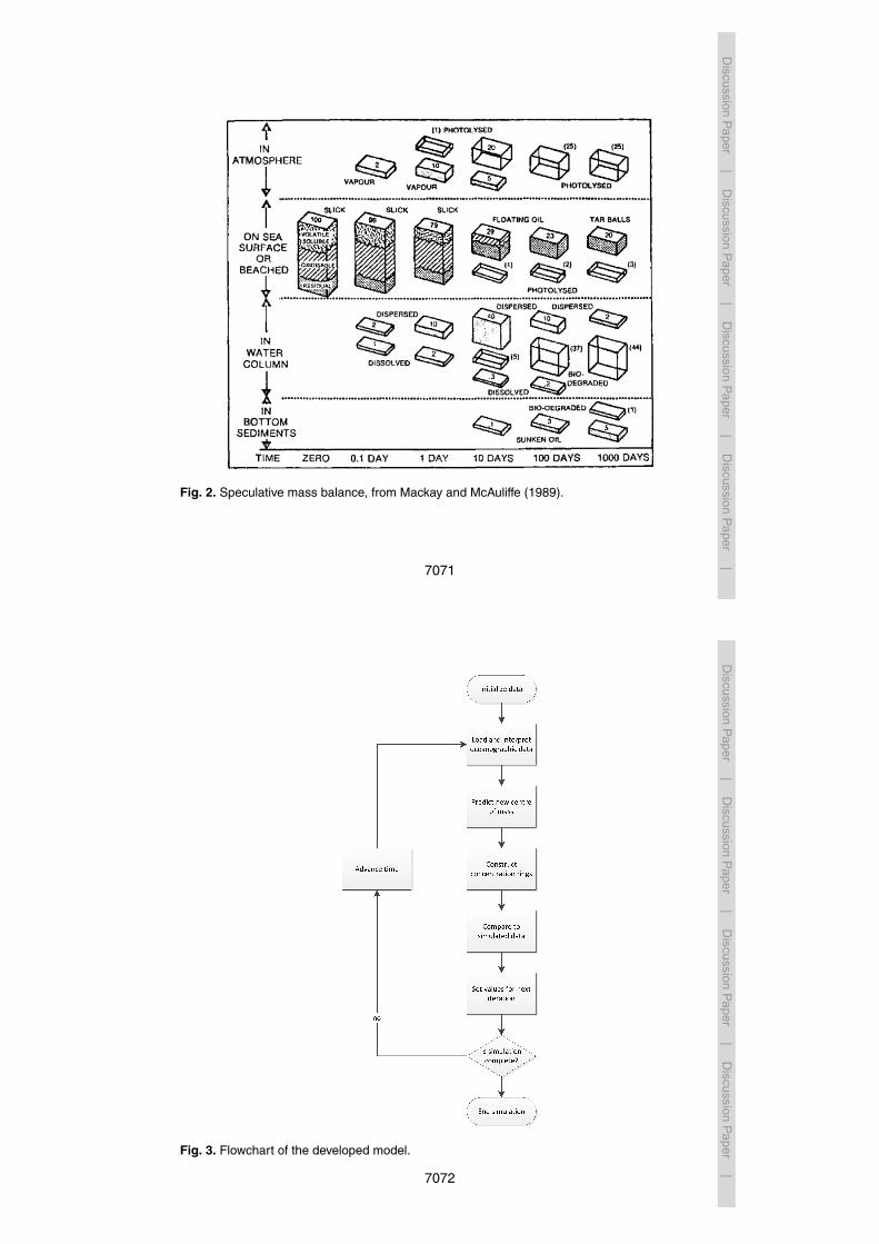
Once the polynomials have been created, it is necessary to outline the developedmethodology for prediction of an oil spill, using the calculated coefficients. The flow5

chart of the developed model can be seen in Fig. 3. The actual code has been writtenin the commercial software package MATLAB® (2011) and the statistics toolbox is usedfor the Monte-Carlo simulation to generate the random numbers.

An overview of the methodology is as follows:

– Interpretation of oceanographic data. The key parameters in the prediction are10

the wind and current velocities. MEDSLIK II produces column structured data forthese from the raw NetCDF files. The prediction code is capable of reading theseand converting them to block structure and converting from latitude and longitudeto metres. A modified version of this code has also been written for the purposes ofMonte-Carlo simulation, where the user inputs a desired wind and current velocity15

directly.

– Centre of mass. To investigate the behaviour of the centre of mass, the wind,current and angle variables have been considered. A polynomial has been devel-oped which links these variables to predict displacement in the x and y planes.The oceanic data is interpolated to find the parameters at the spill location and20

these are fed into the regression model to predict a new centre. Since the cur-rent direction is treated as an axis, the displacement with respect to this is firstcalculated, and then translated into more meaningful coordinates.

– Reconstruction of surface. Now the centre of mass has been predicted, the sur-face reconstruction of the oil spill can be considered. Since this is not linked to25

the destination of the centre of mass, the rings are created around the origin and

7059

Discussion

Paper

|D

iscussionP

aper|

Discussion

Paper

|D

iscussionP

aper|

then displaced by the calculated displacement of the centre of mass. If desired,a contour can then be fitted according to these concentration rings. These are 4thorder polynomials and require the initial spill size (tons) and the spill age (hours).

– Set values for next iteration. For the next time step, it is necessary to set the newcentre of mass for the oil spill. At this stage, the centre of mass can be corrected5

based on observation to produce more accurate results.

5 Case study

In order to validate CranSLIK, it is necessary to investigate its performance when ap-plied to oceanographic conditions. Note the model has been verified against the sam-pled points and over 99.5 % of the oil was captured for each case after 1 h of simulation.10

It was also found that the prediction becomes less accurate for extended periods. Thewind and current velocities were both found to produce near-linear displacement withrespect to time, when considered individually. The developed model works by hourlyprediction which causes cumulative errors in extended simulation. Hindcast modelling,updating the centre of mass every hour, is therefore recommended to minimise error.15

The spill size prediction remains very accurate, above 99 %, over a 36 h period sug-gesting that hindcast modelling is not required to be applied to this part of the code.

5.1 Algeria test case

The case considered uses the oceanographic data for the Algeria spill on the 6 August2008 and a point mass oil spill is released from latitude 38.240◦ and longitude 5.981◦. It20

is found that the proportion of oil captured becomes poor when a full 36 h prediction isperformed, the accuracy rapidly drops after the 4 h mark as shown in Fig. 4. However,under the application of hindcast modelling, where the centre of mass is updated everyhour based on model data, the minimum accuracy is greatly improved. This is likely dueto cumulative errors during prediction. These errors could be present in the developed25

7060

Discussion

Pa

per|

Discussion

Pa

per|

Discussion

Paper

|D

iscussionP

aper|

model, however, since the model has been verified, it may be an error due to theoceanographic data. The model assumes that the oceanographic conditions at thestart of the simulation period are representative of the conditions over the period. Thishowever is not necessarily true and therefore the prediction is less accurate whenthese conditions change greatly over the simulation period. It is possible in this case5

to apply an interpolation since the quantities for the next time step are known howeverthis would not be possible in a real scenario.

Figure 5 shows the displacement error of the centre of mass, when this value isupdated at different intervals. It is clear that the error is far smaller when the simulationis only predicting for an hour and then updating.10

With regards to the spill size only, the accuracy appears to be very good, as seenin Fig. 6. Compared to the accuracy of the centre of mass prediction, this appears tobe far more accurate suggesting that the weakest component of this model is the cen-tre of mass prediction; however the overall accuracy appears to be reasonably good,a minimum of 80 % when hourly prediction is used as seen in Fig. 4. This also justifies15

the decoupling of variables.The supplementary animation shows the predicted oil spill (black rings) and the

MEDSLIK II result (background contour) for a 36 h simulation period for this test case.The centre of mass for the prediction is updated every hour. The lowest proportion ofoil captured is approximately 80 % with the average being about 91 %.20

5.2 Sensitivity analysis

It is also of interest to consider the sensitivity of CranSLIK with respect to the differentinput parameters. This is summarised in Table 3.

The most sensitive variables appear to be the current magnitude and angle. This isexpected since the displacement due to current velocity is far greater than that due to25

the wind velocity, and since the majority of the oil is contained close to the centre, thedispersed elements do not skew the results significantly and hence there is some lee-way with the spill size. This was expected since the current is more displacing than the

7061

Discussion

Paper

|D

iscussionP

aper|

Discussion

Paper

|D

iscussionP

aper|

wind, and it was concluded the wind is less important when the sensitivity of variableswas investigated in MEDSLIK II (De Dominicis et al., 2013a).

5.3 Monte-Carlo simulation

CranSLIK assumes that the wind and current data at the start of the hour are rep-resentative of the full hour. This however is not necessarily true since oceanographic5

conditions may change. Therefore more accurate prediction may be possible if an in-terpolation is applied to the data and expected fields are created. However this is notrelevant for prediction of real-time oil spills. In such scenarios it may be of interest togenerate an expected region for the oil spill.

Due to the incredibly low computational cost required by CranSLIK, a Monte-Carlo10

simulation can be performed in a very low time frame, approximately 1000 simulationsper second on an AMD Phenom II X4 3.6 GHz processor. This can be used to generatean expected region for the oil spill and aid in clean up and recovery operations.

For the Algeria test case, the Monte-Carlo simulation was performed using input dis-tributions developed from the available data. However, due to the 60 h period of data,15

there exists a bimodal peak in the simulation results representative of the alternatingcurrent forcing as shown in Fig. 7. This is present when the simulation is performed us-ing 5000 and 10 000 samples also. This result is not too helpful because of the bimodalpeak. However, it does demonstrate the versatility and robustness of the developedmodel. If the distribution for a location is known, more meaningful results can be pro-20

duced.

5.4 Discussion

Whilst CranSLIK appears to perform well for the tested scenarios, it is necessary toidentify the assumptions made while modelling. Firstly, the displacement of the cen-tre of mass is correlated to the wind and current velocities only, while the spill area25

is determined by the quantity of oil spilled and the age. Although these variables are

7062

Discussion

Pa

per|

Discussion

Pa

per|

Discussion

Paper

|D

iscussionP

aper|

considered dominant, in an fully robust model further simulations considering differentvariables should be performed. This would lead to an even more accurate prediction,however would require more complicated approximations to account for these variablesand their correlations. Secondly, further from MEDSLIK II which was employed, other oilspill prediction codes and softwares may be used and compared identifying their perfor-5

mance in aspects of accuracy and computational effort and at the same time highlightefficiency of the proposed non-intrusive methodology. Finally, only one particular typeof oil spill has been considered: point-mass. Since the developed model moves a cen-tre of mass, and then reconstructs the surface, it is possible to mark several centre ofmasses and predict their destinations. The problem then becomes surface reconstruc-10

tion which would require additional simulations. Also, as with any stochastic problem,additional data could lead to a better regression fit and hence better prediction.

5.5 Technical specifications

The oil spill model code CranSLIK v1.0 is available as an open source code that canbe downloaded together with test case data and output example from the website15

http://public.cranfield.ac.uk/e102081/CranSLIK. CranSLIK is available under the GNUGeneral Public License (GNU-GPL Version 3, 29 June 2007). The code is written inthe commercial software package MATLAB® (2011). The model code can run on anycomputer and operating system that supports Matlab.

6 Conclusions20

This paper describes the development of CranSLIK, a model for the prediction of thedestination and spread of an oil spill via a stochastic approach. The key parameterswere identified as wind velocity, current velocity, spill size and time, and a design squarewas created for the required samples. The simulations were then performed usingMEDSLIK II and regression modelling was applied to create two equations: one to25

7063

Discussion

Paper

|D

iscussionP

aper|

Discussion

Paper

|D

iscussionP

aper|

predict the centre of mass, and one to predict the spill size. The developed code hasbeen presented and discussed. It was then validated against a real test case. Finally,the efficiency of the model is exploited using Monte-Carlo simulation for the purposesof generating maximum likelihood regions. This has limited use when applied to theAlgeria test case due to insufficient data to more accurately fit a distribution.5

The developed model appears to perform well when applied to the Algeria test caseconsidered, with a minimum of 80 % of the oil captured when using hourly predic-tion. The major strength of the developed model is the efficiency and the minimaltime required to perform Monte-Carlo simulation and generate maximum likelihoodregions. However, for this to provide useful results, it is necessary for a distribution10

or a reasonable estimate of expected oceanographic conditions. This paper serves asa demonstration of an alternative method for fast prediction of the advection-diffusion-transformation of an oil spill. The assumptions have been discussed and areas forfurther work highlighted. Whilst the key variables were considered, it has been identi-fied that consideration of additional variables could result in improved accuracy. As with15

all investigations involving stochastic parameters, additional data samples could alsoimprove the results.

Supplementary material related to this article is available online athttp://www.geosci-model-dev-discuss.net/6/7047/2013/gmdd-6-7047-2013-supplement.zip.20

References

ASCE Task Committee on Modelling of Oil Spills of the Water Resources Engineering Division:State-of-the-art review of modelling transport and fate of oil spills, J. Hydraul. Eng., 122,594–609, 1996. 7053

Coppini, G., De Dominicis, M., Zodiatis, G., Lardner, R., Pinardi, N., Santoleri, R., Colella, S.,25

Bignami, F., Hayes, D. R., Soloviev, D., Georgiou, G., and Kallos, G.: Hindcast of oil-spill7064

Discussion

Pa

per|

Discussion

Pa

per|

Discussion

Paper

|D

iscussionP

aper|

pollution during the Lebanon crisis in the Eastern Mediterranean, July–August 2006, Mar.Pollut. Bull., 62, 140–153, 2011. 7056, 7057

De Dominicis, M., Pinardi, N., Zodiatis, G., and Archetti, R.: MEDSLIK-II, a Lagrangian marinesurface oil spill model for short-term forecasting – Part 2: Numerical simulations and vali-dations, Geosci. Model Dev., 6, 1871–1888, doi:10.5194/gmd-6-1871-2013, 2013a. 7049,5

7050, 7056, 7057, 7062De Dominicis, M., Pinardi, N., Zodiatis, G., and Lardner, R.: MEDSLIK-II, a Lagrangian marine

surface oil spill model for short-term forecasting – Part 1: Theory, Geosci. Model Dev., 6,1851–1869, doi:10.5194/gmd-6-1851-2013, 2013b. 7050, 7057

de Prada Gil, M., Gomis-Bellmunt, O., Sumper, A., and Bergas-Jane, J.: Power Generation10

efficiency analysis of offshore wind farms connected to SLPC (simgle large power converter)operated with variable frequencies considering wake effects, Energy, 37, 455–468, 2012.7051, 7055, 7057

Dobricic, S. and Pinardi, N.: An oceanographic three-dimensional variational data assimilationscheme, Ocean Model., 22, 89–105, 2008. 705415

Etkin, D. S.: Analysis of oil spill trends in the United States and worldwide, in: International OilSpill Conference Proceedings, 1291–1300, 2001. 7048

Fay, J. A.: Physical process in the spread of oil on a water surface, Physical-Biological Effects,463–467, doi:10.7901/2169-3358-1971-1-463, 1971. 7052, 7067

Finigas, M., Fieldhouse, B., and Mullin, J.: Water-in-oil emulsion results of formation studies20

and applicability to oil spill modelling, Spill Sci. Technol. B., 5, 81–91, 1999. 7053Graham, B., Reilly, W. K., Beinecke, F., Boesch, D. F., Garcia, T. D., Murray, C. A., and Ulmer, F.:

Deep Water: the Gulf Oil Disaster and the Future of Offshore Drilling, Report to the President,United States Government Printing Office, 2011. 7048

Huang, J. C.: A review of the state-of-the-art of oil spill fate/behaviour models, in: International25

Oil Spill Conference Proceedings, 313–322, 1983. 7053ITOPF: Weathering Process, available at: http://www.itopf.com/marine-spills/fate/

weathering-process/, last access: 13 May 2013. 7051, 7070Li, W., Pang, Y., Lin, J., and Liang, X.: Computational modelling of submarine oil spill with

current and wave by FLUENT, Applied Sciences, Engineering and Technology, 5, 5077–30

5082, 2013. 7049Mackay, D. and McAuliffe, C. D.: Fate of hydrocarbons discharged at sea, Oil and Chemical

Pollution, 5, 1–20, 1989. 7051, 7053, 7071

7065

Discussion

Paper

|D

iscussionP

aper|

Discussion

Paper

|D

iscussionP

aper|

MATLAB®: version 7.12.0.635 (R2011a), The MathWorks Inc., Natick, Massachusetts, 2011.7059, 7063

McGenity, T., Folwell, B., McKew, B., and Sanni, G.: Marine crude-oil biodegradation: a centralrole for interspecies interactions, Aquatic Biosystems, 8, 1–19, doi:10.1186/2046-9063-8-10,2012. 7049, 70505

MEDESS-4MS: Weathering Process, available at: http://www.medess4ms.eu/marine-pollution(last accessed: 13 May 2013). 7051

Miiller, D. E., Holba, A. G., and Hughes, W. B.: Effects of biodegradation on crude oils: sectionII. Characterization, maturation, and degradation, in: Exploration for Heavy Crude Oil andNatural Bitumen: Research Conference, edited by: Meyer, R. F., AAPG Studies in Geology10

Series, 233–241, 1987. 7054Morgan, E. C., Lackner, M., Vogel, R. M., and Baise, L. G.: Probability distributions for offshore

wind speeds, Energy Conservation and Management, 52, 15–26, 2011. 7051, 7055Myers, R. H., Montgomery, D. C., and Anderson-Cook, C. M.: Response Surface Methodology,

3rd Edn., John Wiley and Sons, 2009. 705515

Oddo, P., Adani, M., Pinardi, N., Fratianni, C., Tonani, M., and Pettenuzzo, D.: A nested Atlantic-Mediterranean Sea general circulation model for operational forecasting, Ocean Sci., 5, 461–473, doi:10.5194/os-5-461-2009, 2009. 7054

Pinardi, N. and Coppini, G.: Preface “Operational oceanography in the Mediterranean Sea: thesecond stage of development”, Ocean Sci., 6, 263–267, doi:10.5194/os-6-263-2010, 2010.20

7054Pinardi, N., Allen, I., Demirov, E., De Mey, P., Korres, G., Lascaratos, A., Le Traon, P.-Y., Mail-

lard, C., Manzella, G., and Tziavos, C.: The Mediterranean ocean forecasting system: firstphase of implementation (1998–2001), Ann. Geophys., 21, 3–20, doi:10.5194/angeo-21-3-2003, 2003. 705425

Reed, M., Øistein Johansen, Brandvik, P. J., Daling, P., Lewis, A., Fiocco, R., Mackay, D., andPrentki, R.: Oil spill modeling towards the close of the 20th century: overview of the state ofthe art, Spill Sci. Technol. B., 5, 3–16, 1999. 7049, 7050, 7051

Tonani, M., Pinardi, N., Dobricic, S., Pujol, I., and Fratianni, C.: A high-resolution free-surfacemodel of the Mediterranean Sea, Ocean Sci., 4, 1–14, doi:10.5194/os-4-1-2008, 2008. 705430

US Congress, Office of Technology Assessment: Bioremediation for Marine Oil Spills – Back-ground Paper, Tech. Rep. OTA-BP-O-70, US Government Printing Office, Washington, DC,1991. 7054

7066

Discussion

Pa

per|

Discussion

Pa

per|

Discussion

Paper

|D

iscussionP

aper|

Table 1. Spreading laws for oil spills (Fay, 1971).

1-D (l =) Axisymmetric (r =)

Inertial k1i(∆gAt2)1/3 k2i(∆V t

2)1/4

Viscous k1v(∆gA2t3/2/ν1/2)1/4 k2v(∆gV 2t3/2/ν1/2)1/6

Surface tension k1t(δ2t3/ρ2ν)1/4 k2t(δ

2t3/ρ2ν)1/4

A = volume of oil per unit length normal to x;g = acceleration due to gravity;k = proportionality constants:k1i = k1v = 1.5,k1t = 1.33,k2i = 1.14,k2v = 1.45,k2t = 2.30;l = length of 1-D oil slick;r = maximum radius of axisymmetric oil slick solubility;t = time since initiation of spread;V = volume of oil in axisymmetric spread;x = dimension of direction in 1-D spread;σ = spreading coefficient;ν = kinematic viscosity of water;ρ = density of water;∆ = ratio of density difference between water and oil to density of water.

7067

Discussion

Paper

|D

iscussionP

aper|

Discussion

Paper

|D

iscussionP

aper|

Table 2. Sampled values for centre of mass prediction.

Wind magnitude Current magnitude Angle(in ms−1) (in ms−1) (in radians)

0 0 02.0887 0.0505 π/45.7691 0.1497 π/26.1600 0.2488 3π/47.7913 0.3480 π10.1252 0.4472 –15.2786 0.5464 –

7068

Discussion

Pa

per|

Discussion

Pa

per|

Discussion

Paper

|D

iscussionP

aper|

Table 3. Sensitivity of variables for the first hour of the Algeria scenario. Upper and lower rangesfor 90 % accuracy are given.

Variable Lower limit Upper limit Observed

Wind magnitude −2.0423 9.3860 4.3454Current magnitude 0.0065 0.1130 0.0653Wind angle −2.5844 −0.2280 −1.5202Current angle −1.7279 −0.6605 −1.4048Spill size 163.2 NA 680

7069

Discussion

Paper

|D

iscussionP

aper|

Discussion

Paper

|D

iscussionP

aper|

Fig. 1. Weathering process, from ITOPF (2013).

7070

cranslik v1.0: stochastic prediction of oil spill transport and fate

Documents