cray optimization and performance tools - nersc · • improving performance on hpc systems has...
TRANSCRIPT

Cray Optimization and Performance Tools
Harvey Wasserman Woo-Sun Yang
NERSC User Services Group
Cray XE6 Workshop February 7-8, 2011
NERSC Oakland Scientific Facility

Outline
• Introduction, motivation, some terminology
• Using CrayPat
• Using Apprentice2
• Hands-on lab
2

Why Analyze Performance?
• Improving performance on HPC systems has compelling economic and scientific rationales. – Dave Bailey: Value of improving performance of a single application, 5%
of machine’s cycles by 20% over 10 years: $1,500,000 – Scientific benefit probably much higher
• Goal: solve problems faster; solve larger problems
• Accurately state computational need
• Only that which can be measured can be improved
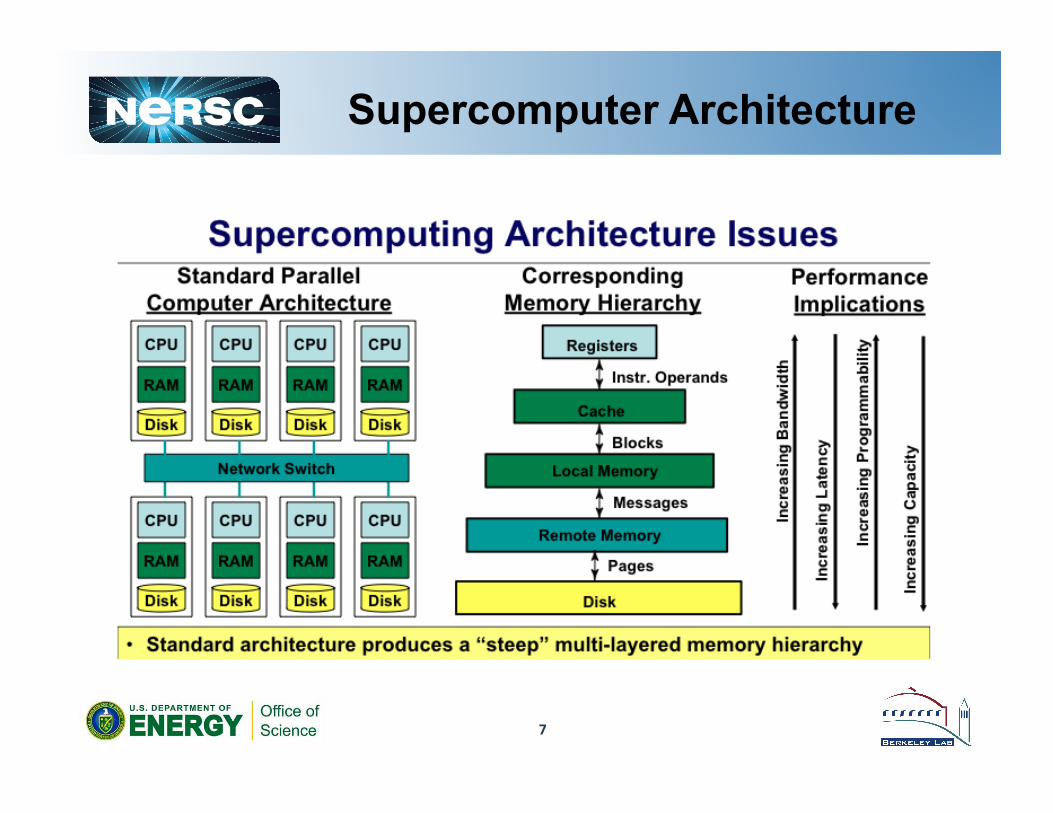
• The challenge is mapping the application to an increasingly more complex system architecture – or set of architectures
3

4
Performance Evaluation as an Iterative Process
Sell Machine
Vendor User
Buy Machine
Improve machine Improve code
Overall goal: more / be.er science results

Performance Analysis Issues
• Difficult process for real codes • Many ways of measuring, reporting • Very broad space: Not just time on one size
– for fixed size problem (same memory per processor): Strong Scaling
– scaled up problem (fixed execution time): Weak Scaling
• A variety of pitfalls abound – Must compare parallel performance to best
uniprocessor algorithm, not just parallel program on 1 processor (unless it’s best)
– Be careful relying on any single number • Amdahl’s Law
5
Performance Questions
• How can we tell if a program is performing well?
• Or isn’t?
• If performance is not “good,” how can we pinpoint why?
• How can we identify the causes?
• What can we do about it?
6
7
Supercomputer Architecture
Performance Metrics
• Primary metric: application time – but gives little indication of efficiency
• Derived measures: – rate (Ex.: messages per unit time,
Flops per Second, clocks per instruction), cache utilization
• Indirect measures: – speedup, efficiency, scalability
8

Performance Metrics
• Most basic: – counts: how many MPI_Send calls? – duration: how much time in MPI_Send ? – size: what size of message in MPI_Send?
• (MPI performance as a function of message size)
9
L =Message Size!
T=Time !
}ts = startup cost !
}tw = cost per word!
Tmsg = ts + twL
= Bandwidth!

Performance Data Collection
• Two dimensions: • When data collection is triggered:
– Externally (asynchronous): Sampling • OS interrupts execution at regular intervals and
records the location (program counter) (and / or other event(s))
– Internally (synchronous): Tracing • Event based • Code instrumentation, Automatic or manual
10

Instrumentation
• Instrumentation: adding measurement probes to the code to observe its execution.
• Different techniques depending on where the instrumentation is added.
• Different overheads and levels of accuracy with each technique
11
User-level abstractions problem domain
source code
source code
object code libraries
instrumentation
instrumentation
executable
runtime image
compiler
linker
OS
VM
instrumentation
instrumentation
instrumentation
instrumentation
instrumentation
instrumentation performance data run
preprocessor
Karl Fuerlinger, UCB

Source-Level Instrumentation
• Goal is to allow performance measurement without modification of user source code
12

Instrumentation
• Instrumentation: adding measurement probes to the code to observe its execution.
• Different techniques depending on where the instrumentation is added.
• Different overheads and levels of accuracy with each technique
13
User-level abstractions problem domain
source code
source code
object code libraries
instrumentation
instrumentation
executable
runtime image
compiler
linker
OS
VM
instrumentation
instrumentation
instrumentation
instrumentation
instrumentation
instrumentation performance data run
preprocessor
Karl Fuerlinger, UCB
Performance Instrumentation
• Approach: use a tool to “instrument” the code 1. Transform a binary executable before
executing 2. Include “hooks” for important events 3. Run the instrumented executable to capture
those events, write out raw data file 4. Use some tool(s) to interpret the data
14

Performance Data Collection
• How performance data are presented: – Profile: combine sampled events over time
• Reflects runtime behavior of program entities – functions, loops, basic blocks – user-defined “semantic” entities
• Good for low-overhead performance assessment • Helps to expose performance hotspots (“bottleneckology”)
– Trace file: Sequence of events over time • Gather individual time-stamped events (and arguments) • Learn when (and where?) events took place on a global timeline • Common for message passing events (sends/receives) • Large volume of performance data generated; generally intrusive • Becomes very difficult at large processor counts, large numbers of
events – Example in Apprentice section at end of tutorial
15

Performance Analysis Difficulties
• Tool overhead • Data overload • User knows the code better than the tool • Choice of approaches • Choice of tools • CrayPat is an attempt to overcome several
of these – By attempting to include intelligence to identify
problem areas – However, in general the problems remain
16
Performance Tools @ NERSC
• IPM: Integrated Performance Monitor • Vendor Tools:
– CrayPat • Community Tools (Not all fully
supported): – TAU (U. Oregon via ACTS) – OpenSpeedShop (DOE/Krell) – HPCToolKit (Rice U) – PAPI (Performance Application Programming
Interface)
17

Profiling: Inclusive vs. Exclusive
• Inclusive time for main: – 100 secs
• Exclusive time for main: – 100-20-50-20=10
secs – Exclusive time
sometimes called “self”
18

USING CRAYPAT
Woo-‐Sun Yang
19

CrayPat Outline
• Introduction • Sampling (and example) • Tracing • .xf files • pat_report • Tracing examples: Heap, MPI, OpenMP • APA (Automatic Program Analysis) • CrayPat API • Monitoring hardware performance counters
• Exercises provided:
20
Exercise info in this box!

Introduction to CrayPat
• Suite of tools to provide a wide range of performance-related information
• Can be used for both sampling and tracing user codes – with or without hardware or network performance
counters
• Supports Fortran, C, C++, UPC, MPI, Coarray Fortran, OpenMP, Pthreads, SHMEM
21
Access to Cray Tools
• Access via module utility • Old:
– module load xt-craypat!– module load apprentice2!
• Now: – module load perftools – xt-craypat, apprentice2, and xt-papi
(via xt-craypat) are loaded
22

Using CrayPat
1. Access the tools – module load perftools!
2. Build your application; keep .o files – make clean!– make!
3. Instrument application – pat_build ... a.out!– Result is a new file, a.out+pat!
4. Run instrumented application to get top time consuming routines – aprun ... a.out+pat!– Result is a new file XXXXX.xf (or a directory containing .xf files)
5. Run pat_report on that new file; view results – pat_report XXXXX.xf > my_profile!– vi my_profile!– Result is also a new file: XXXXX.ap2
23
Adjust script for +pat
CrayPat Notes
• Key points to remember:
– MUST load module prior to building your code • Error message is obscure! ERROR: Missing required ELF section 'link information'
– MUST load module prior to looking at man pages
– MUST run your application in $SCRATCH
– Module name change: xt-craypat perftools
– MUST leave relocatable binaries (*.o) when compiling
24

pat_build for Sampling
• To sample the program counter (PC) at a given time interval or when a specified hardware counter overflows; runs faster than tracing
• To build, use –S or simply without any tracing flag for pat_build – pat_build –S a.out or – pat_build a.out
25
Running a Sampling Experiment
• To run – Set PAT_RT_EXPERIMENT to a type
• Default: samp_pc_time with default time interval (PAT_RT_INTERVAL) of 10,000 microseconds
• Others: samp_pc_ovfl, samp_cs_time, samp_cs_ovfl (see pat man page)
• pat_report on .xf from a sampling experiment generates .apa file (later on this)
26
27
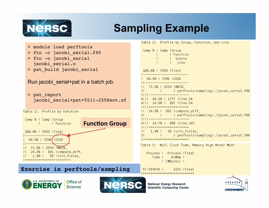
Sampling Example > module load perftools!> ftn -c jacobi_serial.f90!> ftn -o jacobi_serial! jacobi_serial.o!> pat_build jacobi_serial!
Run jacobi_serial+pat in a batch job.
> pat_report! jacobi_serial+pat+5511-2558sot.xf!
Exercise in perftools/sampling!
Func@on Group
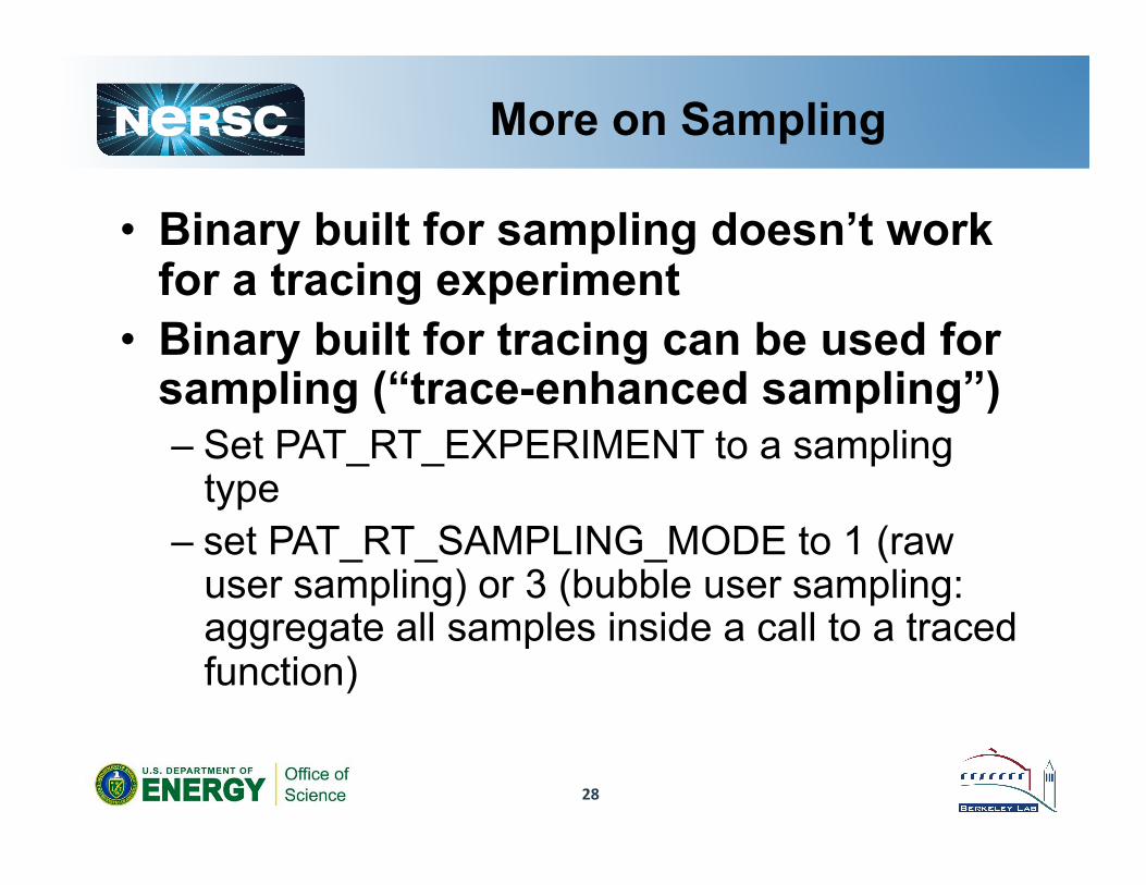
More on Sampling
• Binary built for sampling doesn’t work for a tracing experiment
• Binary built for tracing can be used for sampling (“trace-enhanced sampling”) – Set PAT_RT_EXPERIMENT to a sampling
type – set PAT_RT_SAMPLING_MODE to 1 (raw
user sampling) or 3 (bubble user sampling: aggregate all samples inside a call to a traced function)
28
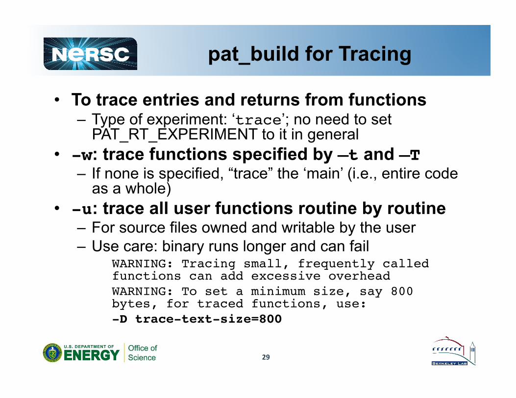
pat_build for Tracing
• To trace entries and returns from functions – Type of experiment: ‘trace’; no need to set
PAT_RT_EXPERIMENT to it in general • -w: trace functions specified by –t and –T!
– If none is specified, “trace” the ‘main’ (i.e., entire code as a whole)
• -u: trace all user functions routine by routine – For source files owned and writable by the user – Use care: binary runs longer and can fail
WARNING: Tracing small, frequently called functions can add excessive overhead!
!WARNING: To set a minimum size, say 800 bytes, for traced functions, use:!
!-D trace-text-size=800!
29

pat_build for Tracing
• -T function: trace function – pat_build –w –T field_,grad_ a.out!– Learn the Unix nm or readelf: nm mycode.o |grep “ T “ !
• -T !function: do not trace function – pat_build -u -T \!field_ a.out!
• trace all user functions except field_ • ‘\’ to escape the ‘!’ character in csh/tcsh
• -t tracefile: trace all functions listed in the file tracefile.
30

• -g: trace all func@ons in certain func@on groups (e.g., MPI): – pat_build -g mpi,heap -u a.out!
– pat_build -g mpi -T \!MPI_Barrier a.out trace all MPI calls except MPI_Barrier
• See $CRAYPAT_ROOT/lib/Trace* for files that list what rou@nes are traced
• mpi
• omp • pthreads • caf • upc • shmem
• ga • heap • blas • blacs • lapack
• scalapack • fftw • petsc • io • netcdf • hdf5 • lustre • adios • sysio • dmapp
• …
31
CrayPat Trace Function Groups

Other pat_build Options
• -f: overwrite an existing instrumented program
• -o instr_prog: – use a different name for the instrumented
executable instead of a.out+pat – can put instr_prog at the end of the command
line without ‘-o’ • -O optfile: use the pat_build options in
the file optfile. – Special argument ‘-O apa’ will be discussed later
Exercise in perftools/pat_build_examples!
32

Instrumenting Programs Using Compiler Options
• Available in Pathscale, GNU, and Cray compilers at NERSC
• Requires recompile, link (selected files) • Alternative to pat_build –u
– GNU, PathScale: cc –finstrument-functions -c pgm.c! cc –o pgm pgm.c!
– Cray compiler: cc –h func_trace -c pgm.c! cc –o pgm pgm.o
– Then pat_build –w pgm!
33

.xf Files
• Experiment data files; binary files • Number of .xf files
– Single file (for ≤ 256 PEs) or directory containing multiple (~√PEs) files
– Can be changed with PAT_RT_EXPFILE_MAX • Name convention
– a.out+pat+<UNIX_PID>-<NODE_ID>[st][dfot].xf (or a.out+apa+….xf; see APA)
– [st][dfot]: [sampling, tracing], [distributed memory, forked process, OpenMP, Pthreads]
• New one each time you run your application • Can create .xf file(s) in other than the current
location by setting PAT_RT_EXPFILE_DIR
34

pat_report
• Generates from .xf data file(s) ASCII text report and .ap2 file (to be viewed with Apprentice2) – Create .ap2 file right after .xf file becomes available!
• .xf file requires the instrumented executable in the original directory (not portable)
• .ap2 doesn’t (self-contained and portable) • pat_report on .xf file (or directory containing
multiple .xf files) generates – text report to stdout (terminal) – .ap2 file – .apa file, in case of a sampling experiment
• Running on .ap2 file generates text report to stdout
35

pat_report Options
• -d: data items to display (time data, heap data, counter data,…)
• -b: how data is aggregated or labeled (group, function, pes, thread, …)
• -s: details of report appearance (aggregation, format,…)
• -O|-b|-d|-s –h: list all available cases for the option!
36
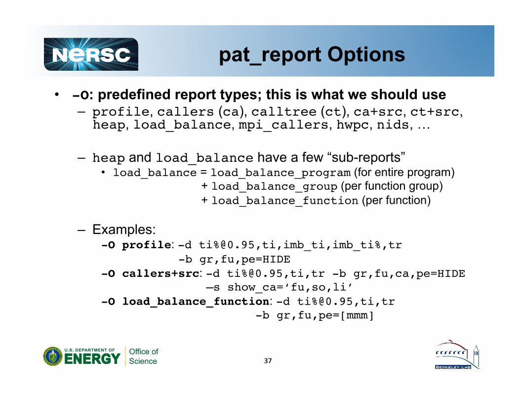
pat_report Options
• -O: predefined report types; this is what we should use!– profile, callers (ca), calltree (ct), ca+src, ct+src, heap, load_balance, mpi_callers, hwpc, nids, …
– heap and load_balance have a few “sub-reports” • load_balance = load_balance_program (for entire program)
+ load_balance_group (per function group) + load_balance_function (per function)
– Examples: -O profile: -d ti%@0.95,ti,imb_ti,imb_ti%,tr! -b gr,fu,pe=HIDE!-O callers+src: -d ti%@0.95,ti,tr -b gr,fu,ca,pe=HIDE! –s show_ca=‘fu,so,li’!-O load_balance_function: -d ti%@0.95,ti,tr!! ! ! ! ! ! ! -b gr,fu,pe=[mmm]!
37

pat_report Options
• Without –d, -b or -O, a few reports appear by default; dependent on the used trace groups
• -i instr_prog: specify the path for the instrumented executable (if not in the same directory as the .xf file)
• -o output_file: specify the output file name • -T: disable all thresholds (5%)
• pat_report lists the options used in the report – a good place to learn options; try adding an option to the existing ones
• By default, all reports (-O) show either no individual PE values or only the PEs having the maximum, median, and minimum values.
• The suffix _all can be appended to any of the pat_report keyword options to show the data for all PEs
38

Exercise in perftools/heap!
39
Heap Memory Example > module load perftools!> ftn -c jacobi_serial.f90!> ftn -o jacobi_serial ! jacobi_serial.o!> pat_build -g heap -u! jacobi_serial!
Run jacobi_serial+pat in a batch job.
> pat_report! jacobi_serial+pat+15243-18tot.xf!
Some@mes not easy to understand
Heap func@on group

• Profiling by MPI func@ons
• MPI message stats
• load imbalance among MPI tasks
> module load perftools!> ftn -c jacobi_mpi.f90!> ftn -o jacobi_mpi! jacobi_mpi.o!> pat_build -g mpi -u jacobi_mpi!
Run jacobi_mpi+pat in a batch job.
> pat_report! jacobi_mpi+pat+15207-18tdt.xf!
40
MPI Code Example
Exercise in perftools/mpi!

per PE
41
MPI Code Example imb = max – avg imb% = imb/max * npes/(npes-1) * 100%
No per-‐PE info PEs with max, min, median values
Func@on Groups

42
MPI Code Example
Bins by message size
per PE
Level of depth
callers

• Time spent wai@ng at a barrier before entering a collec@ve can be a significant indica@on of load imbalance.
• MPI_SYNC group: for @me spent wai@ng at the barrier before entering the collec@ves
• Actual @me spent in the collec@ves go to the MPI func@on group
• Not to separate these groups, set PAT_RT_MPI_SYNC to 0 before aprun
43
MPI_SYNC Function Group

• ‘-O mpi_sm_rank_order!![-s rank_grid_dim=M,N]!![-s rank_cell_dim=m,n]!![-s mpi_dest=d]’:
– Based on sent messages – -s rank_*: specify a
different MPI process topology » Global topology, M×N!» topology per node, m×n!
– consider d busiest partners (default, 8)
MPI Rank Order Suggestion
44
> pat_report -O mpi_sm_rank_order jacobi_mpi+pat+30971-19tdot.xf > ls MPICH_RANK_ORDER.* MPICH_RANK_ORDER.d MPICH_RANK_ORDER.u
Examined the cases 0, 1, 2, and 3 (‘d’ and ‘u’) for MPICH_RANK_REORDER_METHOD; provided MPICH_RANK_ORDER file for the ‘d’ and ‘u’ cases.
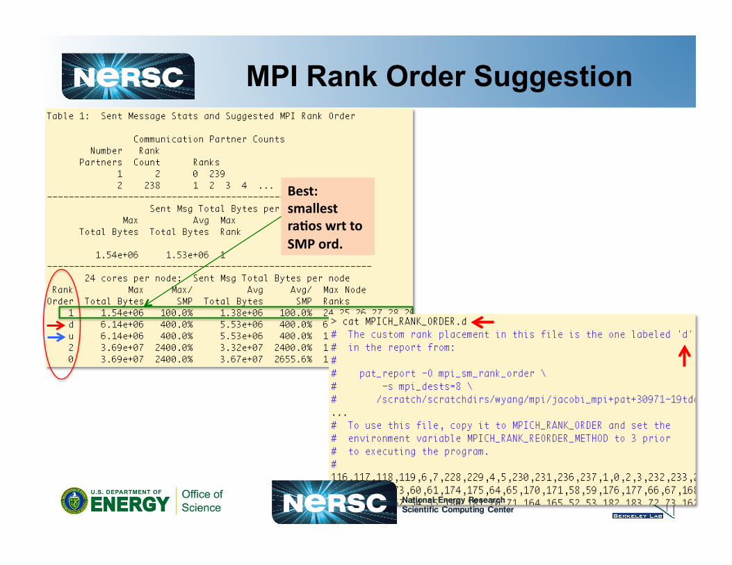
Best: smallest ra@os wrt to SMP ord.
MPI Rank Order Suggestion
45
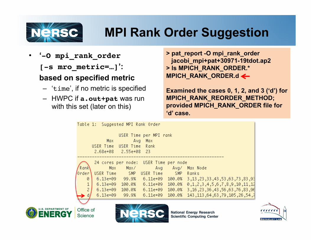
• ‘-O mpi_rank_order !![-s mro_metric=…]’: based on specified metric
– ‘time’, if no metric is specified – HWPC if a.out+pat was run
with this set (later on this)!
MPI Rank Order Suggestion
46
> pat_report -O mpi_rank_order jacobi_mpi+pat+30971-19tdot.ap2 > ls MPICH_RANK_ORDER.* MPICH_RANK_ORDER.d
Examined the cases 0, 1, 2, and 3 (‘d’) for MPICH_RANK_REORDER_METHOD; provided MPICH_RANK_ORDER file for ‘d’ case.

> module load perftools!> ftn -mp=nonuma -c jacobi_omp.f90!> ftn -mp=nonuma -o jacobi_omp! jacobi_omp.o!> pat_build -g omp -u jacobi_omp!
Run jacobi_omp+pat in a batch job
> pat_report! jacobi_omp+pat+15307-18tot.xf!
Exercise in perftools/openmp!
OpenMP Code Example
47

48
OpenMP Code Example
• 24 thread case • Good load balance
in parallel regions!
• Overhead: – Imb. =100%!, all in
the master thread (pat_report’s ‘–O load_balance’ to see this more clearly)
– largest in init_fields_
No per-‐thread info

49
OpenMP Code Example
jacobi_omp.f90 with ngrind=9,600 and maxiter=20

Automatic Program Analysis (APA)
• One may not know in advance where large run time is spent; tracing all the functions can be overwhelming due to large overhead
1. Have the tool detect the most time consuming functions in the application with a sampling experiment
2. Feed this information back to the tool to instrument for focused data collection
3. Get performance information on the most significant parts of the application
• APA does this for you (you can do the same thing by hand)
50

Automatic Program Analysis (APA)
1. pat_build -O apa a.out • Produces the instrumented executable a.out+pat for sampling
2. aprun -n … a.out+pat • Produces data file, e.g., a.out+pat+4677-19sdot.xf
3. pat_report a.out+pat+4571-19sdot.xf • Produces a.out+pat+4571-19sdot.apa (suggested options for tracing) • Produces a.out+pat+4571-19sdot.ap2
4. Edit a.out+pat+4571-19sdot.apa, if necessary (next slide) 5. pat_build -O a.out+pat+4571-19sdot.apa
• Produces a.out+apa for tracing 6. aprun -n … a.out+apa
• Produces a.out+apa+4590-19tdot.xf 7. pat_report a.out+apa+4590-19tdot.xf > out
51
Exercise in perftools/apa!

• Recommended pat_build op@ons for tracing
• Customize it for your need – Include/exclude funcTons – Add/change opTons
• Note that the sugges@ons may not be valid for a very different task/thread configura@on
52
.apa File
PAT_RT_HWPC set to 1
mpi trace group chosen
Trace ‘MAIN_’, but not ‘compute_diff_’
Instrumented program to create Program to instrument
Command to run
Sampling run result
CrayPat Application Program Interface (API)
• Assume your code contains initialization and solution sections
• Want to analyze performance only of solution
• How to do this? Several approaches: – Init section is only one routine (or just a few
routines): eliminate it (or them) from the profile. – Init section is many routines: Use API to define a
profile region that excludes init – What happens if some routines shared by init
and solve? Use API to turn profiling on and off as needed
53
Exercise in perftools/api!

Arbitrary, user-assigned id’s
54
Using the API > module load perftools!> ftn -c jacobi_mpi_api.f90!> ftn -o jacobi_mpi_api jacobi_mpi_api.o!> pat_build -g mpi -u jacobi_mpi_api!
Run jacobi_mpi_api+pat in a batch job. !> pat_report! jacobi_mpi_api+pat+502-19tdot.xf!
Hardware Performance Counters
• Registers available on the processor that count certain events
• Minimal overhead – They’re running all the time – Typically one clock period to read
• Potentially rich source of performance information
55

Types of Counters
• Cycles • Instruction count • Memory references, cache hits/misses • Floating-point instructions • Resource utilization
56

PAPI Event Counters
• PAPI (Performance API) provides a standard interface for use of the performance counters in major microprocessors
• Predefined actual and derived counters supported on the system – To see the list, run ‘papi_avail’ on compute node via aprun:
module load perftools!!!aprun –n 1 papi_avail!
• AMD native events also provided; use ‘papi_native_avail’:
!! !aprun –n 1 papi_native_avail
57

Hardware Performance Monitoring
• Specify hardware counters to be monitored during sampling or tracing – Default is “off” (no HW counters measured) – Choose up to 4 events
• Can specify individual events: setenv PAT_RT_HWPC “PAPI_FP_OPS,PAPI_L1_DCM”! aprun –n … a.out+pat (or a.out+apa)
• Or predefined event group number (next slide): setenv PAT_RT_HWPC 1! aprun –n … a.out+pat (or a.out+apa)
• Multiplexing (monitoring more than 4 events) to be supported in later versions (5.2?)
58
Exercise in perftools/hwpc!

Predefined Counter Groups for PAT_RT_HWPC
0 Summary with instruction metrics 1 Summary with translation lookaside buffer (TLB) metrics 2 L1 and L2 cache metrics 3 Bandwith information 4 *** DO NOT USE, not supported on Quad-core or later AMD Opteron processors *** 5 Floating point instructions 6 Cycles stalled and resources empty 7 Cycles stalled and resources full 8 Instructions and branches 9 Instruction cache values 10 Cache hierarchy 11 Floating point instructions (2) 12 Floating point instructions (vectorization) 13 Floating point instructions (single precision) 14 Floating point instructions (double precision) 15 L3 cache 16 L3 cache, core-level reads 17 L3 cache, core-level misses 18 L3 cache, core-level fills caused by L2 evictions 19 Prefetches
59

Hardware Performance Monitoring
60
PAT_RT_HWPC = 1
Measured
Derived
avg uses (or hits): per word per miss
pat_report –s data_size=4 … (because single precision was used)
cacheline: 64 Bytes L1 cache: 64 KB, dedicated for each core L2 cache: 512 KB, dedicated for each core page: 4 KB (2 MB if huge page)
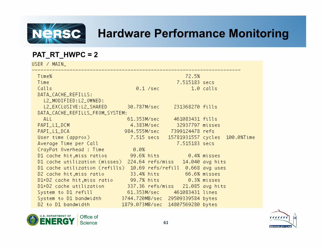
Hardware Performance Monitoring
61
PAT_RT_HWPC = 2

Hardware Performance Monitoring
62
PAT_RT_HWPC = 5
RelaTve raTos for mulTplies and adds

Hardware Performance Monitoring
63
PAT_RT_HWPC = 12
vector length (for sp) for 128-‐bit wide SSE2 vector operaTon = 16583040480 / 4154398320 = 3.99 Compiled with ‘`n –fastsse …’
Add and mulTply instrucTons issued
Adds and mulTplies performed

Guidelines to Identify the Need for Optimization
64
* Suggested by Cray
Derived metric Op@miza@on needed when* PAT_RT_HWPC
ComputaTonal intensity < 0.5 ops/ref 0, 1
L1 cache hit raTo < 90% 0, 1, 2
L1 cache uTlizaTon (misses) < 1 avg hit 0, 1, 2
L1+L2 cache hit raTo < 92% 2
L1+L2 cache uTlizaTon (misses) < 1 avg hit 2
TLB uTlizaTon < 0.9 avg use 1
(FP MulTply / FP Ops) or (FP Add / FP Ops)
< 25% 5
VectorizaTon < 1.5 for dp; 3 for sp 12 (13, 14)

Monitoring Network Performance Counters
• Use PAT_RT_NWPC instead of PAT_RT_HWPC
• See ‘Overview of Gemini Hardware Counters’, S-0025-10 – http://docs.cray.com
65

USING CRAY’S APPRENTICE TOOL
Harvey Wasserman
66

Using Apprentice
• Optional visualization tool for Cray’s perftools data
• Use it in a X Windows environment • Uses a data file as input (XXX.ap2) that is
prepared by pat_report!1. module load perftools!2. ftn -c mpptest.f!3. ftn -o mpptest mpptest.o!4. pat_build -u -g mpi mpptest!5. aprun -n 16 mpptest+pat!6. pat_report mpptest+pat+PID.xf >
my_report!7. app2 [--limit_per_pe tags] [XXX.ap2]!
67

Opening Files
• Identify files on the command line or via the GUI:
68

69
Apprentice Basic View Can select new
(addiTonal) data file and do a screen dump
Can select other views of the data
Worthless Useful
Can drag the “calipers” to focus the view on porTons of the run
70
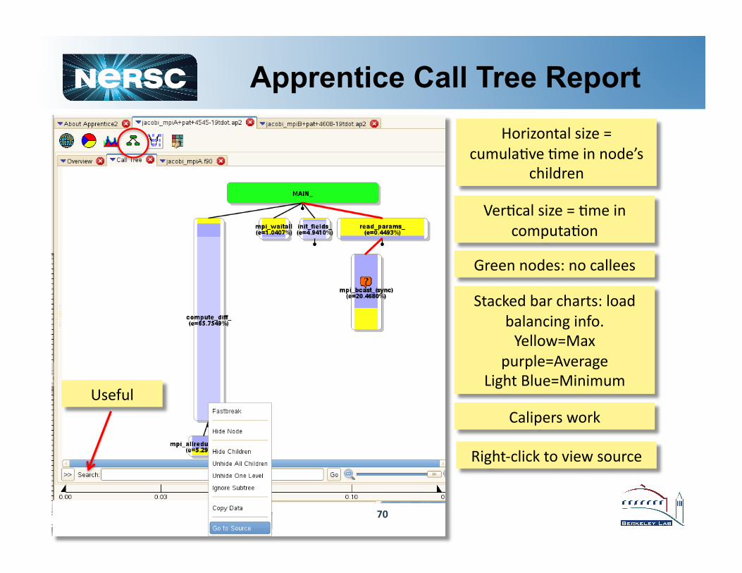
Apprentice Call Tree Report Horizontal size =
cumulaTve Tme in node’s children
VerTcal size = Tme in computaTon
Green nodes: no callees
Stacked bar charts: load balancing info. Yellow=Max
purple=Average Light Blue=Minimum
Calipers work
Right-‐click to view source
Useful

71
Apprentice Call Tree Report Red arc idenTfies path to the highest detected load
imbalance.
Call tree stops there because nodes were filtered out. To see the
hidden nodes, right-‐click on the node a.ached to the marker and select "unhide all children” or "unhide one
level".
Double-‐click on for more info about load
imbalance.

Apprentice Event Trace Views
• Run code with setenv PAT_RT_SUMMARY 0
• Caution: Can generate enormous data files and take forever
72

Apprentice Traffic Report
73
Shows message traces as a funcTon of Tme
Look for large blocks of barriers held up by a single
processor
Zoom is important; also, run just a porTon of your
simulaTon
Scroll, zoom, filter: right-‐click on trace
Click here to select this report

Apprentice Traffic Report: Zoomed
• Mouse hover pops up window showing source location. 74
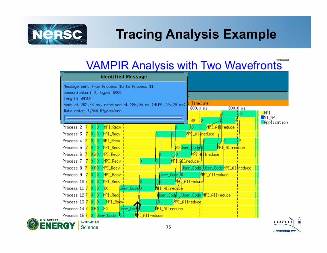
75
Tracing Analysis Example

Mosaic View
•
•
76
Click here to select this report
Can right-‐click here for more opTons
Colors show average Tme (green=low, red=high)
Very difficult to interpret by itself – use the Craypat
message staTsTcs with it.
Shows Interprocessor communicaTon topology and color-‐coded intensity

77
Mosaic View
SP CG
LU
MG
FT BT

NERSC6 Application Benchmark Characteristics
Benchmark Science Area Algorithm Space Base Case Concurrency
Problem Description
CAM Climate (BER) Navier Stokes CFD 56, 240 Strong scaling
D Grid, (~.5 deg resolution); 240 timesteps
GAMESS Quantum Chem (BES)
Dense linear algebra 384, 1024 (Same as Ti-09)
DFT gradient, MP2 gradient
GTC Fusion (FES) PIC, finite difference 512, 2048 Weak scaling
100 particles per cell
IMPACT-T Accelerator Physics (HEP)
PIC, FFT component 256,1024 Strong scaling
50 particles per cell
MAESTRO Astrophysics (HEP)
Low Mach Hydro; block structured-grid multiphysics
512, 2048 Weak scaling
16 32^3 boxes per proc; 10 timesteps
MILC Lattice Gauge Physics (NP)
Conjugate gradient, sparse matrix; FFT
256, 1024, 8192 Weak scaling
8x8x8x9 Local Grid, ~70,000 iters
PARATEC Material Science (BES)
DFT; FFT, BLAS3 256, 1024 Strong scaling
686 Atoms, 1372 bands, 20 iters
78

NERSC6 Benchmarks Communication Topology*
MILC
PARATEC IMPACT-‐T CAM
MAESTRO GTC
79 *From IPM

Sample of CI & %MPI
*CI is the computaTonal intensity, the raTo of # of FloaTng Point OperaTons to # of memory operaTons.
80

For More Information
• Using Cray Performance Analysis Tools, S–2376–51 – http://docs.cray.com/books/S-2376-51/S-2376-51.pdf
• man craypat • man pat_build • man pat_report • man pat_help very useful tutorial program • man app2 • man hwpc • man intro_perftools • man papi • man papi_counters
81

For More Information
• “Performance Tuning of Scientific Applications,” CRC Press 2010
82

83
Exercise
Same code, same problem size, run on the same 24 cores. What is different? Why might one perform be.er than the other? What performance characterisTcs are different?

Exercise
• Get the sweep3d code. Untar • To build: type ‘make mpi’ • Instrument for mpi, user • Get an interactive batch session, 24 cores • Run 3 sweep3d cases on 24 cores creating
Apprentice traffic/mosaic views: – cp input1 input; aprun –n 24 …!– cp input2 input; aprun –n 24 …!– cp input3 input; aprun –n 24 …!
• View the results from each run in Apprentice and try to explain what you see.
84
85
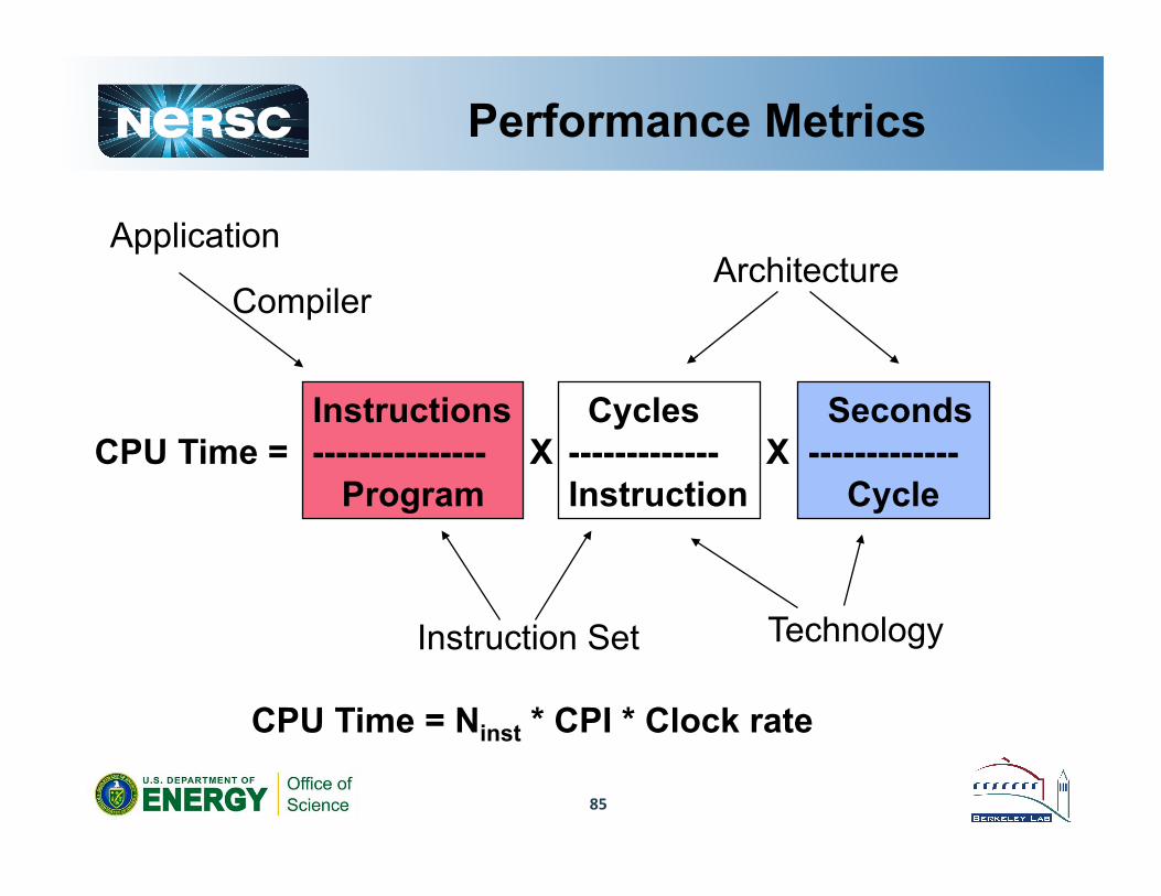
Performance Metrics
CPU Time = Ninst * CPI * Clock rate
Application
Compiler
CPU Time = Instructions --------------- Program
Cycles ------------- Instruction
Seconds ------------- Cycle
X X
Instruction Set
Architecture
Technology