101

Creating SCS Curve Number Grid using HEC-GeoHMS

Prepared by

Venkatesh Merwade

School of Civil Engineering, Purdue University

vmerwade@purdue.edu

September 2012

Introduction

SCS curve number grid is used by many hydrologic models to extract the curve number for

watersheds. The objective of this tutorial is to use soil and land use data to create a curve number

grid using HEC-GeoHMS (ArcGIS 10 version).

Computer Requirements

You must have a computer with latest windows operating system, and the following programs

installed:

1. ArcGIS 10 (ArcView)

2. Hec-GeoHMS for ArcGIS 10

You can download the HEC-GeoHMS version from the following link:

http://www.hec.usace.army.mil/software/hec-geohms/download.html

You will need to have administrative access to install Arc Hydro and HEC-GeoHMS.

Data Requirements and Description

This tutorial requires the following datasets:

(1) DEM for the study area

(2) SSURGO soil data

(3) 2006 land cover grid from USGS

The DEM and land cover grid from USGS and SSURGO data for Cedar Creek in northeast

Indiana are provided as zip file at the end of this paragraph. The SSURGO soil data that will be

used is provided in a geodatabase (cedar_ssurgo.mdb) that is created in the “Downloading

SSURGO Soil Data” tutorial available at:

(http://web.ics.purdue.edu/~vmerwade/education/download_ssurgo.pdf). You can look at the

SSURGO download tutorial if you want to learn how this dataset is processed. Also, if you are

interested in downloading the DEM and land cover data by yourself, instructions are available in

the following tutorial: http://web.ics.purdue.edu/~vmerwade/education/ned_nhd.pdf

It is highly recommended that you go through these exercises of downloading the data to make

yourself aware of the procedure involved.

102

(Notes:

1. The DEM, land use and soil data used in this tutorial are already clipped to the Cedar Creek

study watershed

2. This tutorial uses the SSURGO soil data, which is the highest resolution soil data available in

public domain from NRCS. This can be replaced by STATSGO data as long as you know

how to interpret STATSTO to follow the steps provided in this tutorial)

Download the data from ftp://ftp.ecn.purdue.edu/vmerwade/download/data/cngrid.zip

Unzip cngrid.zip in your working directory. The ArcCatalog-view of the data folder (or

whatever name you gave to your working folder) is shown below:

cedar_ssurgo is the geodatabase with SSURGO spatial and tabular data for cedar creek area.

cedar_dem is the raw 30 DEM for Cedar Creek obtained from USGS and clipped for the study

watershed, and cedar_lu is the 2001 land cover grid from USGS. All datasets have a common

spatial reference (NAD_1983_UTM_16).

Note: It is very critical to assign and use consistent coordinate system for all the datasets.

Getting Started

Open ArcMap. Create a new empty map, and save it as cngrid.mxd (or any other name). Add

Spatial Analyst extension and activate it by clicking on CustomizeExtensions…, and

checking the box next to Spatial Analyst.

Preparing land use data for CN Grid

Add cedar_luse grid to the map document. You will see the grid is added with a unique

symbology assigned to cells having identical numbers as shown below:

103

These numbers represent a land use class defined according to the USGS land cover institute

(LCI). A description of some of the land classes and their associated numbers in the grid is

shown below by reproducing LCI webpage (http://landcover.usgs.gov/classes.php). You can visit

LCI website (publications link) to learn more about how the land use grid is created.

104

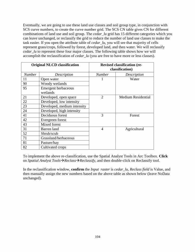
Eventually, we are going to use these land use classes and soil group type, in conjunction with

SCS curve numbers, to create the curve number grid. The SCS CN table gives CN for different

combinations of land use and soil group. The cedar_lu grid has 15 different categories which you

can leave unchanged, or reclassify the grid to reduce the number of land use classes to make the

task easier. If you open the attribute table of cedar_lu, you will see that majority of cells

represent grass/crops, followed by forest, developed land, and then water. We will reclassify

cedar_lu to represent these four major classes. The following table shows how we will

accomplish the reclassification of cedar_lu (you are free to have more or less classes).

Original NLCD classification Revised classification (re-

classification)

Number Description Number Description

11 Open water 1 Water

90 Woody wetlands

95 Emergent herbaceous

wetlands

21 Developed, open space 2 Medium Residential

22 Developed, low intensity

23 Developed, medium intensity

24 Developed, high intensity

41 Deciduous forest 3 Forest

42 Evergreen forest

43 Mixed forest

31 Barren land 4

Agricultural

52 Shrub/scub

71 Grassland/herbaceous

81 Pasture/hay

82 Cultivated crops

To implement the above re-classification, use the Spatial Analyst Tools in Arc Toolbox. Click

on Spatial Analyst ToolsReclassReclassify, and then double-click on Reclassify tool.

In the reclassification window, confirm the Input raster is cedar_lu, Reclass field is Value, and

then manually assign the new numbers based on the above table as shown below (leave NoData

unchanged).

105

Save the output raster as lu_reclass in your working folder, and click OK. A new grid named

lu_reclass will be added to the map as shown below (you may not get the same colors in

symbology which is OK)

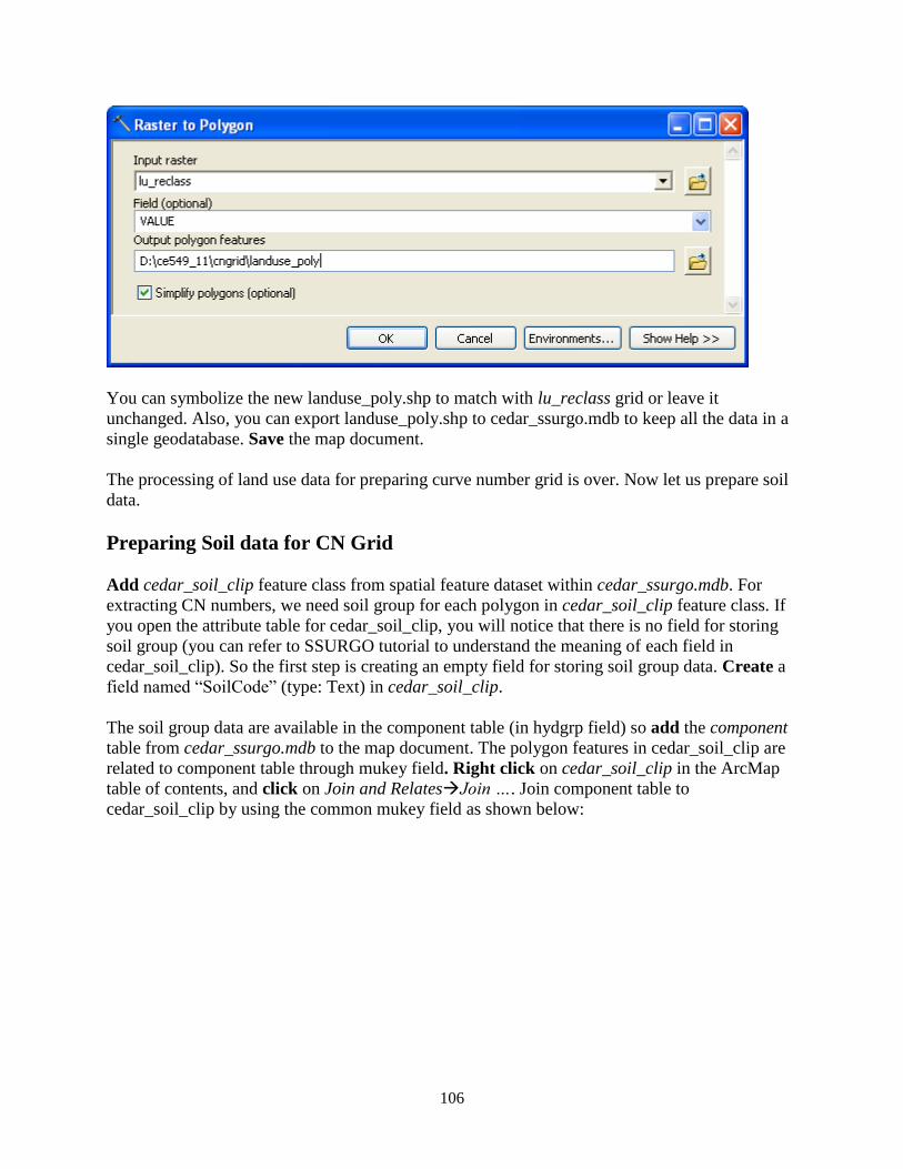
The final step in processing land use data is converting the reclassified land use grid into a

polygon feature class which will be merged with soil data later. In ArcToolbox, Click on

Conversion ToolsFrom RasterRaster to Polygon. Confirm the Input raster is lu_reclass, the

Field is Value, output geometry type is Polygon, and save the Output features as

landuse_poly.shp in your working directory (this output is saved only as a shapefile without any

other options). Click OK.

106

You can symbolize the new landuse_poly.shp to match with lu_reclass grid or leave it

unchanged. Also, you can export landuse_poly.shp to cedar_ssurgo.mdb to keep all the data in a

single geodatabase. Save the map document.

The processing of land use data for preparing curve number grid is over. Now let us prepare soil

data.

Preparing Soil data for CN Grid

Add cedar_soil_clip feature class from spatial feature dataset within cedar_ssurgo.mdb. For

extracting CN numbers, we need soil group for each polygon in cedar_soil_clip feature class. If

you open the attribute table for cedar_soil_clip, you will notice that there is no field for storing

soil group (you can refer to SSURGO tutorial to understand the meaning of each field in

cedar_soil_clip). So the first step is creating an empty field for storing soil group data. Create a

field named “SoilCode” (type: Text) in cedar_soil_clip.

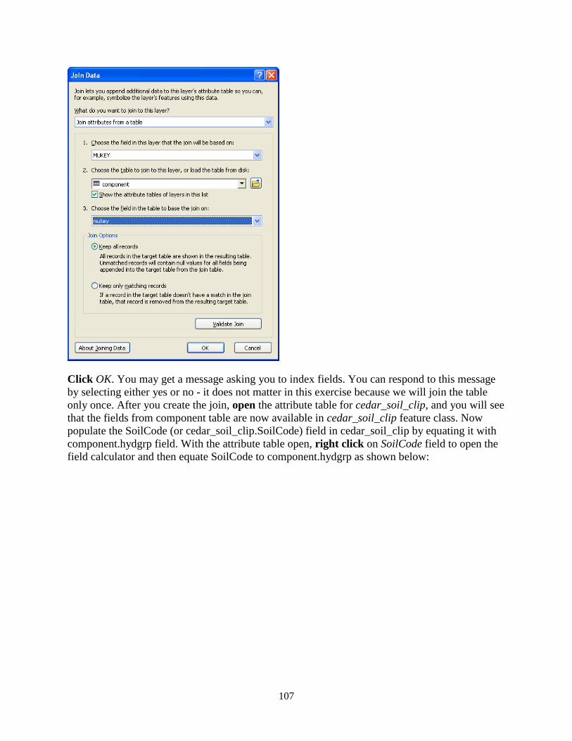
The soil group data are available in the component table (in hydgrp field) so add the component

table from cedar_ssurgo.mdb to the map document. The polygon features in cedar_soil_clip are

related to component table through mukey field. Right click on cedar_soil_clip in the ArcMap

table of contents, and click on Join and RelatesJoin …. Join component table to

cedar_soil_clip by using the common mukey field as shown below:

107

Click OK. You may get a message asking you to index fields. You can respond to this message

by selecting either yes or no - it does not matter in this exercise because we will join the table

only once. After you create the join, open the attribute table for cedar_soil_clip, and you will see

that the fields from component table are now available in cedar_soil_clip feature class. Now

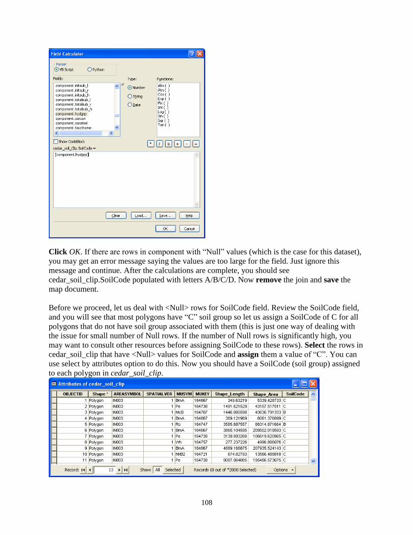
populate the SoilCode (or cedar_soil_clip.SoilCode) field in cedar_soil_clip by equating it with

component.hydgrp field. With the attribute table open, right click on SoilCode field to open the

field calculator and then equate SoilCode to component.hydgrp as shown below:

108

Click OK. If there are rows in component with “Null” values (which is the case for this dataset),

you may get an error message saying the values are too large for the field. Just ignore this

message and continue. After the calculations are complete, you should see

cedar_soil_clip.SoilCode populated with letters A/B/C/D. Now remove the join and save the

map document.

Before we proceed, let us deal with <Null> rows for SoilCode field. Review the SoilCode field,

and you will see that most polygons have “C” soil group so let us assign a SoilCode of C for all

polygons that do not have soil group associated with them (this is just one way of dealing with

the issue for small number of Null rows. If the number of Null rows is significantly high, you

may want to consult other resources before assigning SoilCode to these rows). Select the rows in

cedar_soil_clip that have <Null> values for SoilCode and assign them a value of “C”. You can

use select by attributes option to do this. Now you should have a SoilCode (soil group) assigned

to each polygon in cedar_soil_clip.

109

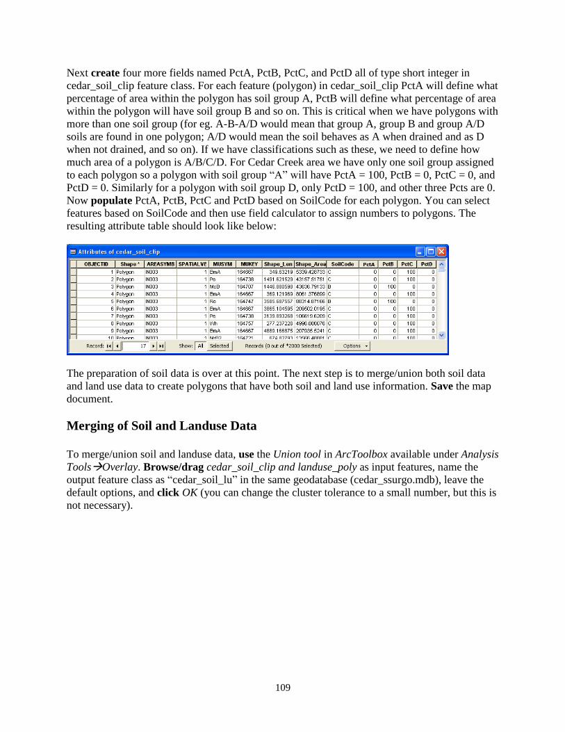
Next create four more fields named PctA, PctB, PctC, and PctD all of type short integer in

cedar_soil_clip feature class. For each feature (polygon) in cedar_soil_clip PctA will define what

percentage of area within the polygon has soil group A, PctB will define what percentage of area

within the polygon will have soil group B and so on. This is critical when we have polygons with

more than one soil group (for eg. A-B-A/D would mean that group A, group B and group A/D

soils are found in one polygon; A/D would mean the soil behaves as A when drained and as D

when not drained, and so on). If we have classifications such as these, we need to define how

much area of a polygon is A/B/C/D. For Cedar Creek area we have only one soil group assigned

to each polygon so a polygon with soil group “A” will have PctA = 100, PctB = 0, PctC = 0, and

PctD = 0. Similarly for a polygon with soil group D, only PctD = 100, and other three Pcts are 0.

Now populate PctA, PctB, PctC and PctD based on SoilCode for each polygon. You can select

features based on SoilCode and then use field calculator to assign numbers to polygons. The

resulting attribute table should look like below:

The preparation of soil data is over at this point. The next step is to merge/union both soil data

and land use data to create polygons that have both soil and land use information. Save the map

document.

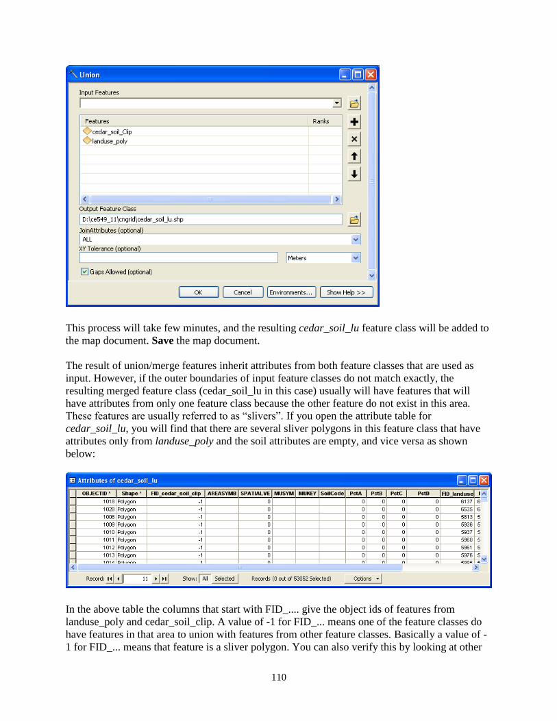
Merging of Soil and Landuse Data

To merge/union soil and landuse data, use the Union tool in ArcToolbox available under Analysis

ToolsOverlay. Browse/drag cedar_soil_clip and landuse_poly as input features, name the

output feature class as “cedar_soil_lu” in the same geodatabase (cedar_ssurgo.mdb), leave the

default options, and click OK (you can change the cluster tolerance to a small number, but this is

not necessary).

110

This process will take few minutes, and the resulting cedar_soil_lu feature class will be added to

the map document. Save the map document.

The result of union/merge features inherit attributes from both feature classes that are used as

input. However, if the outer boundaries of input feature classes do not match exactly, the

resulting merged feature class (cedar_soil_lu in this case) usually will have features that will

have attributes from only one feature class because the other feature do not exist in this area.

These features are usually referred to as “slivers”. If you open the attribute table for

cedar_soil_lu, you will find that there are several sliver polygons in this feature class that have

attributes only from landuse_poly and the soil attributes are empty, and vice versa as shown

below:

In the above table the columns that start with FID_.... give the object ids of features from

landuse_poly and cedar_soil_clip. A value of -1 for FID_... means one of the feature classes do

have features in that area to union with features from other feature classes. Basically a value of -

1 for FID_... means that feature is a sliver polygon. You can also verify this by looking at other

111

fields. For example features that have FID_cedar_soil_clip = -1 have attributes only from

landuse_poly and all attributes from cedar_soil_clip = 0.

One way to deal with sliver polygons is to assign missing values to all features. Another way

(easiest!) is to just delete them. For this exercise we will take the easy route, but you may want to

populate these features for other studies depending on your project needs.

Start the Editor. Select all the features that have “FID_...” = -1 and delete them. Save your

edits, stop the Editor, and save the map document.

This finishes the processing of spatial data for creating the curve number grid. The next step is to

prepare a look-up table that will have curve numbers for different combinations of land uses and soil

groups. In this case, we will use SCS curve numbers that are available from literature (SCS reports, or

SCS tables from text books). The spatial features in conjunction with the look-up table can then be used

to create curve number grid.

Creating CN Look-up table

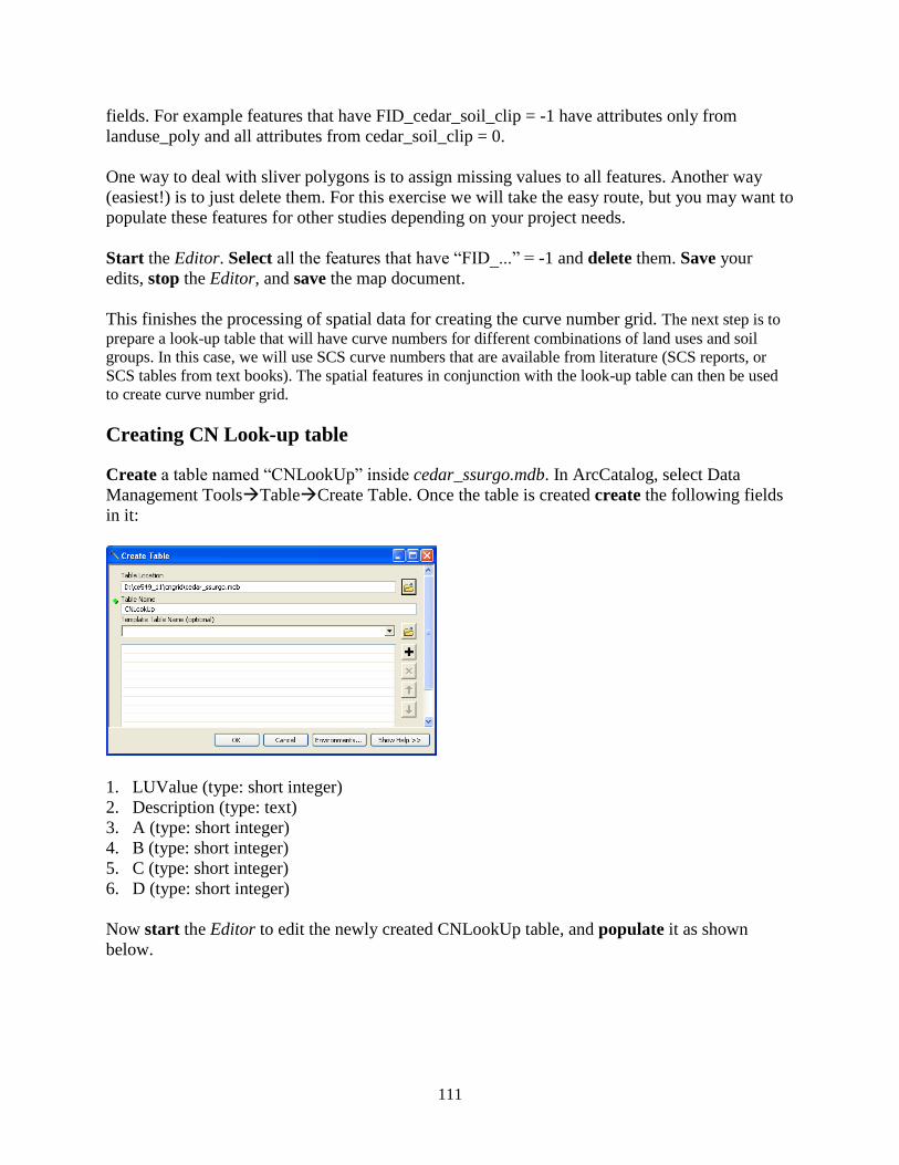
Create a table named “CNLookUp” inside cedar_ssurgo.mdb. In ArcCatalog, select Data

Management ToolsTableCreate Table. Once the table is created create the following fields

in it:

1. LUValue (type: short integer)

2. Description (type: text)

3. A (type: short integer)

4. B (type: short integer)

5. C (type: short integer)

6. D (type: short integer)

Now start the Editor to edit the newly created CNLookUp table, and populate it as shown

below.

112

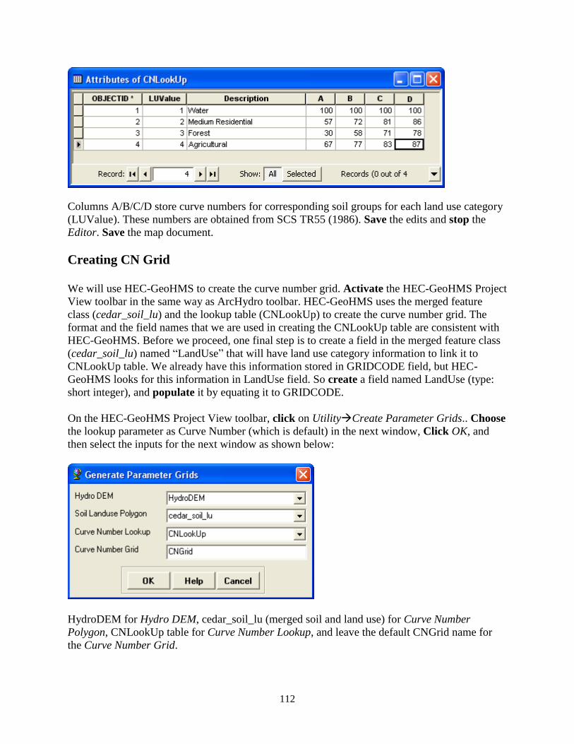
Columns A/B/C/D store curve numbers for corresponding soil groups for each land use category

(LUValue). These numbers are obtained from SCS TR55 (1986). Save the edits and stop the

Editor. Save the map document.

Creating CN Grid

We will use HEC-GeoHMS to create the curve number grid. Activate the HEC-GeoHMS Project

View toolbar in the same way as ArcHydro toolbar. HEC-GeoHMS uses the merged feature

class (cedar_soil_lu) and the lookup table (CNLookUp) to create the curve number grid. The

format and the field names that we are used in creating the CNLookUp table are consistent with

HEC-GeoHMS. Before we proceed, one final step is to create a field in the merged feature class

(cedar_soil_lu) named “LandUse” that will have land use category information to link it to

CNLookUp table. We already have this information stored in GRIDCODE field, but HEC-

GeoHMS looks for this information in LandUse field. So create a field named LandUse (type:

short integer), and populate it by equating it to GRIDCODE.

On the HEC-GeoHMS Project View toolbar, click on UtilityCreate Parameter Grids.. Choose

the lookup parameter as Curve Number (which is default) in the next window, Click OK, and

then select the inputs for the next window as shown below:

HydroDEM for Hydro DEM, cedar_soil_lu (merged soil and land use) for Curve Number

Polygon, CNLookUp table for Curve Number Lookup, and leave the default CNGrid name for

the Curve Number Grid.

113

This process takes a while (actually quite a while!). Be patient and CNGrid will be added to your

map document. You can change the symbology of the grid to make it look pretty!

You now have a very useful dataset for use in several hydrologic models and studies. Save the

map document, and exit ArcMap.

OK. You are done!

114