CREATING USEFUL PRODUCTS FROM

CONNECTICUT’S 2000 LIDAR DATA SET

October 2008

Thomas H. Meyer

JHR 08-314 Project 07-2

This research was sponsored by the Joint Highway Research Advisory Council (JHRAC) of the University of Connecticut and the Connecticut Department of Transportation and was performed through the Connecticut Transportation Institute of the University of Connecticut.

The contents of this report reflect the views of the authors who are responsible for the facts and accuracy of the data presented herein. The contents do not necessarily reflect the official views or policies of the University of Connecticut or the Connecticut Department of Transportation. This report does not constitute a standard, specification, or regulation.

i

Technical Report Documentation Page1. Report No. 2. Government Accession No. 3. Recipient’s Catalog No.

JHR 08-314 N/A 4. Title and Subtitle 5. Report Date

October 2008

6. Performing Organization Code

Creating Useful Products From Connecticut’s 2000 LIDAR Data Set

N/A

7. Author(s) 8. Performing Organization Report No.

Thomas H. Meyer JHR 08-314 9. Performing Organization Name and Address 10. Work Unit No. (TRAIS)

N/A University of Connecticut

11. Contract or Grant No. Connecticut Transportation Institute Storrs, CT 06269-5202

N/A 12. Sponsoring Agency Name and Address 13. Type of Report and Period Covered

FINAL Connecticut Department of Transportation

14. Sponsoring Agency Code 280 West Street Rocky Hill, CT 06067-0207

N/A

15. Supplementary Notes

This study was conducted under the Connecticut Cooperative Highway Research Program (CCHRP, http://www.cti.uconn.edu/chwrp/index.php). 16. Abstract

The State of Connecticut owns a LIght Detection and Ranging (LIDAR) data set that was collected in 2000 as part of the State’s periodic aerial reconnaissance missions. Although collected eight years ago, these data are just now becoming ready to be made available to the public. These data constitute a massive “point cloud”, being a long list of east-north-up triplets in the State Plane Coordinate System Zone 0600 (SPCS83 0600), orthometric heights (NAVD 88) in US Survey feet. Unfortunately, point clouds have no structure or organization, and consequently they are not as useful as Triangulated Irregular Networks (TINs), digital elevation models (DEMs), contour maps, slope and aspect layers, curvature layers, among others. The goal of this project was to provide the computational infrastructure to create a first cut of these products and to serve them to the public via the World Wide Web. The products are available at http://clear.uconn.edu/data/ct_lidar/index.htm.

17. Key Words 18. Distribution Statement

LIDAR; shapefile; TIN; DEM; contour lines

No restrictions. This document is available to the public through the National Technical Information Service Springfield, Virginia 22161

19. Security Classif. (of this report) 20. Security Classif. (of this page) 21. No. of Pages 22. Price

Unclassified Unclassified 33 N/A

Form DOT F 1700.7 (8-72) Reproduction of completed page authorized

ii

iii

Table of Contents 1 BACKGROUND ........................................................................................................ 1 2 OBJECTIVE ............................................................................................................... 3 3 METHODS ................................................................................................................. 4 4 QUALITY CHECK RESULTS.................................................................................. 4

4.1 Duplicate Postings .............................................................................................. 4 4.2 Negative Heights................................................................................................. 5 4.3 Data Dropout....................................................................................................... 6 4.4 Posting Density ................................................................................................... 6

5 RESULTS ................................................................................................................... 7 6 RECOMMENDATIONS............................................................................................ 7

6.1 Additional interface options................................................................................ 7 6.2 Follow-on products and formats ......................................................................... 8 6.3 Recommendations for future vendor requirements............................................. 8

7 Appendix A............................................................................................................... 10

iv

List of Figures Figure 1. A schematic of a whiskbroom, side scanning LIDAR…………………………2 Figure 2.a. LIDAR samples taken from the intersection of Route 32 and Route 44. The intersection is in the center of the samples. The irregular spacing of the samples is clearly evident as are some cultural features……………………………………………………………………....3 Figure 2.b. shows a TIN of the samples in Fig. 2.a. with a vertical exaggeration of three……....3 Figure 3. Number of duplicate postings per quarter-Quarter quadrangle………………...4 Figure 4. Number of postings per quarter-quarter quadrangle with negative heights (in 10,000’s of postings)………………………………………………………………………5 Figure 5. Posting dropouts in the NE-NE quarter-quarter of the Coventry quadrangle….6 Figure 6. Postings per quarter-quarter quadrangle in 1000’s of postings………………...7

v

List of Tables Table 1. Typical ALTMS Operation Parameters………………………………………….2

vi

Definitions or Glossary of Terms ALTMS (Airborne Laser Topographic Mapping System) see LIDAR. DEM (Digital Elevation Model) a raster of elevation samples that capture the topographic information of some area of interest. LIDAR (LIght Detection and Ranging) is an instrument carried in an airborne (or orbiting) platform that moves the LIDAR over the area of interest to collect topographic elevation samples TIN (Triangulated Irregular Network) A tessellation of triangular facets created among triplets of topographic samples forming a three-dimensional model of the topographic surface.

vii

1 BACKGROUND

A LIDAR is an instrument carried in an airborne (or orbiting) platform that moves the LIDAR over the area of interest to collect topographic elevation samples (Baltsavias 1999a; Baltsavias 1999b). Also known as an airborne laser topographic mapping system (ALTMS), a LIDAR is a laser coupled to timing hardware such that the laser emits a pulse of energy that propagates through the air beneath the platform until the pulse strikes an opaque object. Some of the pulse is usually reflected back to the sensor where its time-of-flight is determined and recorded. The time-of-flight multiplied by the speed of light is twice the range to the object that reflected the pulse. The location and orientation (attitude) of the platform are monitored and recorded so as to provide the position and orientation of the sensor at the moment the sample was taken. This information provides the necessary geometry to completely determine the location of the object that reflected the pulse.

A single pulse can result in zero, one or more returns. Zero returns result from a pulse either being fully absorbed by some object in the environment (called targets), such as a water body, or from too few photons being reflected back to the laser detector to be discernable above background noise. In either case, no returns are infrequent. Single returns occur when the pulse is reflected by some target like the ground or a building. The LIDAR flown by TerraPoint was a multi-return sensor, meaning that it has the technical capability of detecting more than one return from a single pulse. A single pulse returns in multiple returns if the pulse is reflected by a complex target such as a tree. The laser pulse has a discrete width on the ground, called a beam spot which, in this case, was on average around 0.9 m in diameter. When a pulse propagates through the limbs of a tree, a return can be reflected from every opaque object intercepting the pulse, including the ground, assuming the pulse was not entirely intercepted by the tree. The TerraPoint LIDAR used for this mission is a first-return, last-return instrument, meaning that it records the first and last returns seen by the detector hardware. LIDARs exist that record the entire return waveform (Wright and Brock 2002a; Wright and Brock 2002b).

The laser is directed out of the platform and into the environment by means of rotating or oscillating mirrors that sweep the beam away from the direction of motion. There are several different methods of doing this (Baltsavias 1999a) but the TerraPoint LIDAR utilized a whiskbroom scanner, being an oscillating mirror which created a sinusoidal scan of sample locations, see Fig. 1. The angle of the beam relative to the nadir is the side scan angle and the rate at which the beam is directed across the flight path is the scan rate.

1

Figure 1. A schematic of a helical scan LIDAR showing overlapping flight lines.

LIDARs collect samples rapidly. Modern LIDARs can collect over 90,000 samples per

second (90 kHz) (Optech 2003) although the TerraPoint LIDAR collected samples at 20 kHz. The density of the samples on the ground is determined by the sampling rate, the platform’s velocity and altitude, and the angle at which the beam spot is directed off nadir. Table 1, which was taken from a TerraPoint document delivered to CT DOT (Appendix A), provides the operational parameters.

Table 1. Typical ALTMS Operating Parameters

Collection altitude 914 m AGL Ground speed 140 knots Laser swath width 594 m (65% of flying height) Shot rate 20 kHz Scan rate 49 Hz Cross track spacing (uniform across swath) 1.5 m Along track spacing (uniform along track) 1.5 m Nominal X/Y ground sample size 0.9 m diameter laser spot footprint X, Y, Z positional accuracy RMSE absolute 0.5 m (X, Y), 0.3 m (Z)

As shown in Table 1, the Connecticut data set was created nominally with sub-meter

sample spacing. However, the State purchased a thinned, “mowed” data set, meaning that returns from non-topographic features (e.g., buildings, trees) were removed, in theory. The purchased data were supposed to have a nominal sample spacing of 20 feet (one sample in 400 sq. ft). With this sampling density and taking the area of Connecticut to be 4845 sq. miles, there should be roughly 335 million samples in the data set. The delivered data require nearly five gigabytes of storage. Figure 2.a. shows some samples from the USGS Coventry 7.5 minute topographic map illustrating the irregular pattern formed by

2

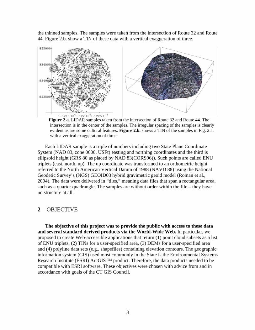
the thinned samples. The samples were taken from the intersection of Route 32 and Route 44. Figure 2.b. show a TIN of these data with a vertical exaggeration of three.

Figure 2.a. LIDAR samples taken from the intersection of Route 32 and Route 44. The intersection is in the center of the samples. The irregular spacing of the samples is clearly evident as are some cultural features. Figure 2.b. shows a TIN of the samples in Fig. 2.a. with a vertical exaggeration of three.

Each LIDAR sample is a triple of numbers including two State Plane Coordinate

System (NAD 83, zone 0600, USFt) easting and northing coordinates and the third is ellipsoid height (GRS 80 as placed by NAD 83(CORS96)). Such points are called ENU triplets (east, north, up). The up coordinate was transformed to an orthometric height referred to the North American Vertical Datum of 1988 (NAVD 88) using the National Geodetic Survey’s (NGS) GEOID03 hybrid gravimetric geoid model (Roman et al., 2004). The data were delivered in “tiles,” meaning data files that span a rectangular area, such as a quarter quadrangle. The samples are without order within the file – they have no structure at all.

2 OBJECTIVE

The objective of this project was to provide the public with access to these data

and several standard derived products via the World-Wide Web. In particular, we proposed to create Web-accessible applications that return (1) point cloud subsets as a list of ENU triplets, (2) TINs for a user-specified area, (3) DEMs for a user-specified area and (4) polyline data sets (e.g., shapefiles) containing elevation contours. The geographic information system (GIS) used most commonly in the State is the Environmental Systems Research Institute (ESRI) ArcGIS ™ product. Therefore, the data products needed to be compatible with ESRI software. These objectives were chosen with advice from and in accordance with goals of the CT GIS Council.

3

3 METHODS

During prototype development, it was discovered that the ERSI data formats are

proprietary and that the Arc family of GIS software does not readily import data in formats other than its native form. This caused the processing to be shifted away from a multi-processor LINUX Beowulf cluster to a standard Intel multi-core desktop. We were not able to use standard programming methods to develop the data products because we had to use ArcGIS itself to create them due to the proprietary data format obstacle. Therefore, we designed and created ArcGIS processing scripts in the Python programming language to perform the product creation. Python is platform independent and should, in theory, run the same way on any platform that runs the ArcGIS environment in which the Python runs.

The data were subdivided along to US Geological Survey (USGS) 7.5’ topographic map (quad sheet) boundaries, as is done with many other State geomatics data products. However, even the thinned LIDAR data set typically has over one million postings in a single quad. This is far too much data for most users. Furthermore, most areas of interest are likely to be smaller than an entire 7.5’ region. Therefore, it was decided to subdivide the data into quarter-quarter quadrangle tiles.

The data products produced were “raw” data, ESRI point shapefiles of the postings, ESRI contour line shape files, ESRI digital elevation model coverages, quarter-quarter quadrangle boundary polygons, and ESRI triangulated irregular networks. The “raw” data are ASCII files of the eastings, northings, and heights, as opposed to the actual unprocessed observables of the instruments.

4 QUALITY CHECK RESULTS

The flights covered an area of approximately 4845 sq. miles, encompassing 1620 out

of the 1936 quarter-quarter quadrangles covering Connecticut; many quarter-quarter quadrangles are entirely over water in the Long Island Sound and, thus have no postings. The data were expected to have a nominal data density of 20’ separation between postings for an excepted 351 million postings overall. 197,631,227 postings were actually delivered for an average of 26’ average separation. Sampling revealed posting separations between 24’ and 70’, many duplicated points, postings with negative heights, and areas of significant erroneous data dropout. Culling duplicated or erroneous postings left 195,232,878. This is roughly 56% of the original expected data. Duplicated and erroneous points were omitted before deployment.

4.1 Duplicate Postings The delivered data set had 660,672 exactly duplicate postings (meaning identical

easting, northing, and height values), and an additional 182 postings with identical eastings and northings but different heights. These duplicates were not randomly distributed, but clustered mainly in the western half of the state. Some quarter-quarter quads had more than 12,000 duplicate points each (see Fig. 3). It is possible that the

4

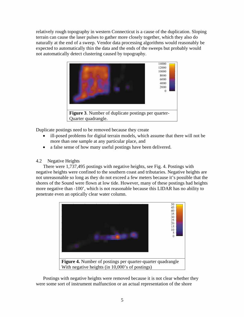
relatively rough topography in western Connecticut is a cause of the duplication. Sloping terrain can cause the laser pulses to gather more closely together, which they also do naturally at the end of a sweep. Vendor data processing algorithms would reasonably be expected to automatically thin the data and the ends of the sweeps but probably would not automatically detect clustering caused by topography.

Figure 3. Number of duplicate postings per quarter- Quarter quadrangle.

Duplicate postings need to be removed because they create

• ill-posed problems for digital terrain models, which assume that there will not be more than one sample at any particular place, and

• a false sense of how many useful postings have been delivered.

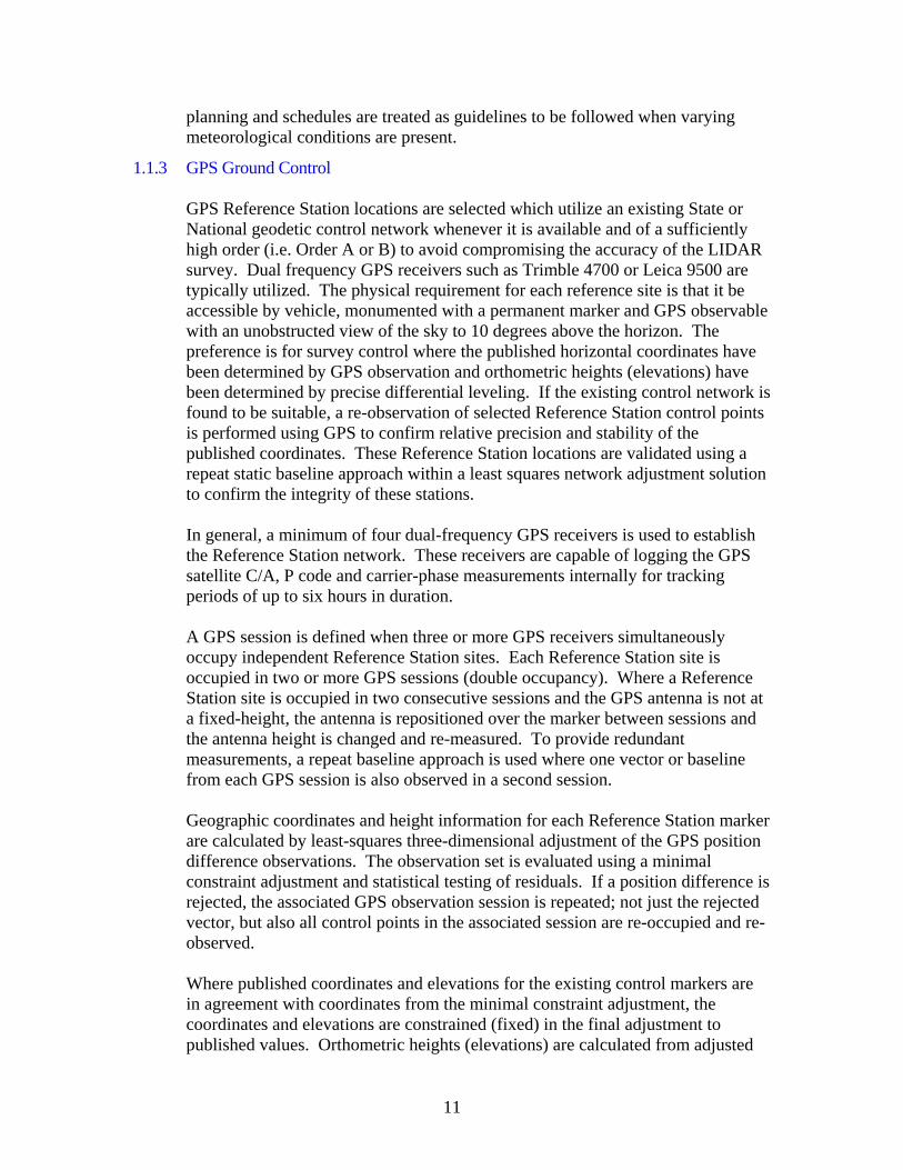
4.2 Negative Heights There were 1,737,495 postings with negative heights, see Fig. 4. Postings with

negative heights were confined to the southern coast and tributaries. Negative heights are not unreasonable so long as they do not exceed a few meters because it’s possible that the shores of the Sound were flown at low tide. However, many of these postings had heights more negative than -100’, which is not reasonable because this LIDAR has no ability to penetrate even an optically clear water column.

Figure 4. Number of postings per quarter-quarter quadrangle With negative heights (in 10,000’s of postings)

Postings with negative heights were removed because it is not clear whether they

were some sort of instrument malfunction or an actual representation of the shore

5

exposed at low tide. We felt it was better to risk omitting a few, albeit interesting, postings along the shore rather than distribute data whose meaning is uncertain.

4.3 Data Dropout LIDAR can be expected to penetrate tree canopies quite well in leaf-off conditions.

Even so, it is reasonable to expect somewhat lower posting densities in areas of dense tree coverage. What is not reasonable is to have large, systematic areas with no coverage. Fig. 5 shows the posting of the NE-NE Coventry quadrangle. The swath down the center extents over four entire quadrangles and appears to be, perhaps, missing flight lines. The vendor’s aircraft flew flight lines guided by a Global Positioning System (GPS) navigation unit, which should be expected to have positional accuracy on the order of meters. Unless the data were flown in severe cross winds, it is hard to blame this on navigation error.

Figure 5. Posting dropouts in the NE-NE quarter-quarter of the Coventry quadrangle.

4.4 Posting Density The expected posting density was 20’ but testing revealed the actual density to vary

between 24’ and 75’ per quarter-quarter quadrangle (see Fig. 6).

6

Figure 6. Postings per quarter-quarter quadrangle in 1000’s of postings.

The posting densities are difficult to interpret. Duplicate removal would be one source of the lower densities in the west. Lower densities in the east could be caused somewhat by large areas of data drop out. However, the mixture of the highest densities with the lowest in areas of apparently homogeneous surface characteristics has no clear explanation.

5 RESULTS

Web pages were created to allow public downloading of the data. The general portal is at the Center for Land Use Education and Research (CLEAR) at http://clear.uconn.edu/. The data description is at http://clear.uconn.edu/data/ct_lidar/index.htm and the data portal at http://clear2.uconn.edu/ct_lidar/ct_lidar_processed-001/index.html. There are zipped archives for each quarter-quarter quad holding the data.

6 RECOMMENDATIONS

Future work should include a thorough quality check of the data, an expanded user interface, and research in to higher-order product creation.

6.1 Additional interface options Subdividing the data into quarter-quarter quadrangles was convenient for the automation of these products but is not very convenient for most users, who would prefer a point-and-click interactive map interface. It would be reasonable to extend this functionality to include drawing a rectangle of interest, a center point and radius, or some political boundary to extract the data. The current method does, however, provide exactly the right infrastructure to make additional, more sophisticated interfaces easy to implement. All that is needed is some flexibility in describing the quarter-quarter quads, then stitching the underlying tiles together.

The graphical user interface (GUI) is envisioned to present the user with “pyramid layers,” so that the terrain model changes resolution as the user views the data with smaller scales. TINs would be retrievable at the different resolutions. Multiresolution TINs are an area of active research (Tsai 1993; Cohen and Dyn 1996; Kidner et al. 2000;

7

Balmelli et al. 2003; Yang et al. 2005). Intelligent, automatic posting thinning would be needed to adjust data set size according to the extent of the user’s area of interest.

6.2 Follow-on products and formats Raw data, point clouds, DEMs, TINs, and contours constitute a minimal set of interesting data products. Research into LIDAR data algorithms already includes automatic building extraction, forest mensuration, road extraction, and waterway routing. To maximize the benefit of the State’s data, additional higher-order data sets such as these should be explored.

There is a sequence to be followed before the most advanced products can be created. For the Connecticut data set, the next step should be automatic void and edge detection. This serves several purposes. First, it will allow detecting data drop out areas in current and future data sets. Knowing the location and extent of problem areas gives the State valuable knowledge with negotiating with vendors and validating products. It also permits follow-on research projects to investigate melding data set from different sources with the intent of “repairing” missing data or leveraging all data sets for a particular area. Second, a natural product of such a project would be the automatic delineation of shorelines and islands, which are clearly useful. It should be noted that location of the legal shoreline is based on the opinion of a licensed surveyor and probably could not be established by these methods. The legal shoreline is much more complicated that what geometry can establish and includes tidal information, among other things.

There are other useful data formats besides those defined by ESRI, including the MicroStation formats favored by engineers. It is recommended investigating creating these data products in both formats to generate products that are useful to the greatest number of Connecticut geomatics professionals.

6.3 Recommendations for future vendor requirements 1. The vendor should be required to remove fully redundant postings. 2. The vendor should separate out postings with duplicated horizontal coordinates but

distinct heights into a separate category. The posting with the lowest elevation should remain in the general data set.

3. Improvements are warranted in the daily quality check requirements and procedures written in to specifications and contracts with future vendors for LIDAR flights (see Appendix A, Section 1.1.10).

4. The vendor should delete postings with unrealistic negative heights.

8

Reference List

Balmelli, L., Liebling, T. and Vetterli, M. 2003. Computational analysis of mesh simplification using global error. Computational Geometry 25 (3): 171-196.

Baltsavias, E.P. 1999a. Airborne laser scanning: basic relations and formulas. ISPRS Journal of Photogrammetry & Remote Sensing 54 (2-3): 199-214.

Baltsavias, E.P. 1999b. A comparison between photogrammetry and laser scanning. ISPRS Journal of Photogrammetry & Remote Sensing 54: 83-94.

Cohen, A. and Dyn, N. 1996. Nonstationary Subdivision Schemes and Multiresolution Analysis. SIAM Journal on Mathematical Analysis 27 (6): 1745-1769.

Kidner, D.B., Ware, J.M., Sparkes, A.J. and Jones, C.B. 2000. Multiscale terrain and topographic modelling with the implicit TIN. Transactions in GIS 4 (4): 361-408.

Meyer, T.H. In Press. Fast algorithms using minimal data structures for common topological relationships in large, irregularly-spaced topographic data sets. Computers & Geosciences .

Meyer, T.H., Eriksson, M. and Maggio, R.C. 2001. Gradient Estimation from Irregularly Spaced Data Sets. Mathematical Geology 33 (6): 693-717.

Optech. 2003. Want more choice? Optech's ALTM gives you 70,000 Hz. http://www.optech.on.ca/pdf/ALTM3070.pdf.

Roman, D. R.; Wang, Y. M.; Henning, W.; and Hamilton, J. (2004). "Assessment of the New National Geoid Height Model, GEOID03." Surveying and Land Information Science, 64(3), pp. 153-162.

Tsai, V.J.D. 1993. Delaunay triangulations in TIN creation: an overview and a linear-time algorithm. Geographical Information Systems 7 (6): 501-524.

Wright, C. Wayne and Brock, John C. 2002a. EAARL: A LIDAR for mapping shallow coral reefs and other coastal environments. In the Seventh International Conference on Remote Sensing for Marine and Coastal Environments, Miami, FL, pp. on cd-rom.

Wright, C. Wayne and Brock, John C. 2002b. A lidar for mapping shallow coral reefs and other coastal environments. in Seventh International Conference on Remote Sensing for Marine and Coastal Environments, Miami, FL.

Yang, B., Shi, W. and Li, Q. 2005. A dynamic method for generating multi-resolution TIN models. Photogrammetric Engineering and Remote Sensing 71 (8): 917-926.

9

7 Appendix A.

1 TerraPoint Data Collection and Processing

1.1 Raw Data Collection

1.1.1 Field Operations

Field operations for the data acquisition phase of the project involves planning flight line coverage, aircraft operations, ground control and calibration as well as logistics for moving personnel and equipment in and out of the project area. The initial project planning is performed at TerraPoint’s main office. As the data acquisition phase gets underway, however, many of the day-to-day decisions are delegated to the personnel at the project site. They have the most complete knowledge of the local environment and are authorized to respond to changing conditions as needed to ensure efficient operations. TerraPoint’s Project Manager maintains close supervision over all activities in the field, and receives daily progress reports communicating the current status and describing any issues that need to be addressed.

1.1.2 Flight Planning

Flight line planning is based on existing maps of the project area and any existing DTM data sets supplemented with auxiliary information on local flight constraints. Some of the factors that are considered include ground terrain, location of cities, location of airports, airport flight patterns, etc. Flight lines are plotted on digitized maps utilizing the ESRI suite of products so that the coordinates of flight lines can be used in the aircraft’s flight management and navigation system. Flight line profiles are generated to aid the pilot and operator in visualizing expected flight conditions prior to the mission.

The primary concern of flight operations planning is the safety of the flight crew and the aircraft. Air Traffic Control (ATC) centers at airports in or near the project area are contacted to determine any flight restrictions that may limit flight operations. Alternate airports and runways in the project area are identified and visited to determine if these facilities could be used in an emergency situation. Another important function of flight operations planning is computing GPS satellite visibility models to determine flight exclusion times when there are not enough GPS satellites to track or the PDOP (Positional Dilution of Precision) values are out of tolerance. TerraPoint will only collect LIDAR data when it is possible to track a minimum of 6 GPS satellites with a PDOP of less than 6.0. Due to the ever-changing satellite geometry, TerraPoint will fly multiple day or night operations during optimum periods of GPS coverage, weather permitting. The flight operations planner will schedule flights to maximize the mission length given the constraints of PDOP, local ATC operations and local terrain considerations. LIDAR flights are subject to weather restrictions, so flight

10

planning and schedules are treated as guidelines to be followed when varying meteorological conditions are present.

1.1.3 GPS Ground Control

GPS Reference Station locations are selected which utilize an existing State or National geodetic control network whenever it is available and of a sufficiently high order (i.e. Order A or B) to avoid compromising the accuracy of the LIDAR survey. Dual frequency GPS receivers such as Trimble 4700 or Leica 9500 are typically utilized. The physical requirement for each reference site is that it be accessible by vehicle, monumented with a permanent marker and GPS observable with an unobstructed view of the sky to 10 degrees above the horizon. The preference is for survey control where the published horizontal coordinates have been determined by GPS observation and orthometric heights (elevations) have been determined by precise differential leveling. If the existing control network is found to be suitable, a re-observation of selected Reference Station control points is performed using GPS to confirm relative precision and stability of the published coordinates. These Reference Station locations are validated using a repeat static baseline approach within a least squares network adjustment solution to confirm the integrity of these stations.

In general, a minimum of four dual-frequency GPS receivers is used to establish the Reference Station network. These receivers are capable of logging the GPS satellite C/A, P code and carrier-phase measurements internally for tracking periods of up to six hours in duration.

A GPS session is defined when three or more GPS receivers simultaneously occupy independent Reference Station sites. Each Reference Station site is occupied in two or more GPS sessions (double occupancy). Where a Reference Station site is occupied in two consecutive sessions and the GPS antenna is not at a fixed-height, the antenna is repositioned over the marker between sessions and the antenna height is changed and re-measured. To provide redundant measurements, a repeat baseline approach is used where one vector or baseline from each GPS session is also observed in a second session. Geographic coordinates and height information for each Reference Station marker are calculated by least-squares three-dimensional adjustment of the GPS position difference observations. The observation set is evaluated using a minimal constraint adjustment and statistical testing of residuals. If a position difference is rejected, the associated GPS observation session is repeated; not just the rejected vector, but also all control points in the associated session are re-occupied and re-observed. Where published coordinates and elevations for the existing control markers are in agreement with coordinates from the minimal constraint adjustment, the coordinates and elevations are constrained (fixed) in the final adjustment to published values. Orthometric heights (elevations) are calculated from adjusted

11

ellipsoid heights and geoid-ellipsoid separations are determined using the geoid model adopted by the National Geodetic Survey (NGS). The variance-covariance matrix is re-scaled by the calculated a posteriori variance factor to provide a more realistic estimate of the relative precision between markers.

To achieve the highest vertical accuracy, enhanced field procedures and data collection techniques are employed. These enhanced field procedures utilize a network of control markers with a grid spacing that does not exceed 30 km. If there is an insufficient number of suitable Ground Control Points (GCPs), additional GCPs are established and surveyed as needed throughout the project area, tying them into the existing network. Candidate sites are reconnoitered for suitability of stability, GPS occupation, accessibility and security. These ancillary stations are observed in a series of two to three hour static GPS sessions as per accepted NGS - Survey Control Specifications with respect to GPS network procedures. These points are also used in a quality control survey as local Reference Stations for any kinematic GPS that may be included within a 10-km proximity of the Station. The amount of feature pick-up for these areas is dependent on the accessibility of the locations and the scheduled session time. These kinematic points serve as QC points around each of the Secondary Station areas for qualifying the LIDAR data accuracy. During LIDAR data collection, at least two GPS ground stations per mission are used. Typically, one is centrally located in the acquisition area (within a 30 km radius) and the second is on an adjacent control monument, which is utilized as an alternate if a problem occurs with the original Reference Station during data collection. This alternate Station is typically less than 30 km from the main GPS Reference Station and is utilized in the daily ground control check aspect of the data collection.

Additional control points are established at the airport selected for the ALTMS base of operations. These points are located in an area free of electronic interference and in a location at the airport where the survey aircraft can have access at any time of the day or night. These control points are incorporated into the network adjustment and are used for static initializations at the start and end of each LIDAR mission.

1.1.4 Calibration Site

The establishment of one or more LIDAR calibration sites for each project is a key element in assuring the highest quality of deliverable data. A calibration site is an area of survey control that is flown over at least one time during every mission. Whenever possible, the calibration site is flown at the beginning and at the end of each mission, in opposite directions, to provide redundancy and a measure of systematic drift. In post-processing, surface values derived from the LIDAR data are tested against the known calibration control points to determine

12

the correct adjustment parameters for each mission. This process immediately identifies any systematic issues in data acquisition or failures on the part of the GPS, IMU or other equipment that may not have been evident to the LIDAR operator during the mission. The calibration site is ideally selected in a relatively open, tree-less area where several large buildings are located. An effective calibration site contains a minimum of three multi-plane roofed buildings spread out over approximately 80 percent of the nominal scan width specified for the project. This separation ensures a good solution on the azimuth orientation of the calibration.

These buildings should have “clean” edges (i.e., free of railings and other overhanging appendages) with a minimum height displacement at their edge of 2 meters to the nearest surface. Each roof surface should be large enough to permit at least five laser points to strike it along the narrowest direction. If the nominal laser point spacing is 1.5 meters, the minimum size for each building roof plane is 7.5 meters by 7.5 meters, although much larger areas are desirable. Each building should also be comprised of multiple roof plane areas (at least two). A typical location for a calibration site meeting these requirements is a small local airfield with multiple hangars, preferably the same one where the ALTMS operations will be staged, provided that permission can be obtained to regularly fly over this area.

The buildings used for calibration are surveyed using both GPS and conventional survey methods. A local network of GPS points are established to provide a baseline for conventional traversing around the perimeter of the buildings. The building edges, peaks and slope intersection points are measured. A theodolite or total station is employed in surveying the roof corners of these buildings. Due to roof overhangs and the difficulty in directly accessing the roofs, the horizontal coordinates for the roof corners are determined primarily from direction measurements and the height of corners by zenith (vertical angle) observations. Each roof corner must be visible from three of the traverse or control points to provide for check (redundant) measurements. In addition to height of instrument, direction and zenith measurements, the horizontal distances to building corners are also measured if the roof overhang cannot be accounted for. The conventional data is logged and used in conjunction with the established GPS baselines. These observations are processed using survey coordinate geometry software that performs a least squares adjustment for determination of point coordinates and height.

1.1.5 Ground Truth Validation Points

Ground truth validation is used to assess the data quality and consistency over sample areas of the project. To facilitate a confident evaluation, existing survey control is used to validate the ALTMS data. Published survey control, where the orthometric height (elevation) has been determined by precise differential leveling observation, is deemed to be suitable.

13

At least three existing NGS stations are occupied each day of the LIDAR survey. These stations are observed using NGS standards for static GPS positioning and are referenced to the main GPS Reference Station providing the static control for that LIDAR mission. In addition to these supplemental stations, the TerraPoint field staff may visit and selectively utilize other existing survey control as well as vehicle mounted kinematic GPS techniques, within 10 km of a surveyed station, for collecting data on selected roadways. Ground truth validation points may be collected for each terrain category to establish RMSE accuracies for the LIDAR project. These points must be gathered in flat or uniformly sloped terrain (<20% slope) away from surface features such as stream banks, bridges or embankments. If collected, these points will be used during data processing to test the RMSE accuracy of the final LIDAR data products.

1.1.6 Data Collection Missions

A LIDAR data collection mission is considered to encompass a single take-off and landing of the aircraft and sensor. The accuracy of data acquired during each mission depends not only on the activities occurring during the flight, but also on a series of pre- and post-flight operations.

1.1.7 Pre-Flight Operations

Prior to each data acquisition mission, a static initialization of the onboard dual frequency GPS receiver is conducted. If a Reference Station has been established at or near the airport, which is the desired procedure, a static initialization period of at least 15 minutes provides sufficient accuracy. If the aircraft and the nearest Reference Station are separated by more than three kilometers, however, the 15-minute static initialization period is increased by an amount proportional to the separation between the aircraft and the Reference Station. This ensures that cycle ambiguities can be resolved to integer values in post-processing of the GPS phase data. The GPS static initialization is performed while the aircraft is stationary, the engines are off and the aircraft is parked away from any GPS antenna obstructions. The pilot and ALTMS operator remain outside the aircraft during initialization to minimize antenna movement. The dual frequency GPS receiver and data logger operate on battery power so that there is no requirement for aircraft power. GPS pseudo-range and phase measurements are logged at a one-second-measurement rate. At the end of the initialization period, the aircraft is cleared for the pilot and ALTMS operator to re-enter the aircraft. The pilot then enables internal aircraft power and permits the ALTMS operator to begin initialization of the complete LIDAR system. When local facilities permit, a TerraPoint supplied external Ground Power Unit (GPU) is connected to the

14

local ac network or to a local generator. The GPU supplies power through the aircraft’s auxiliary power connector to eliminate drain on the aircraft battery. If this is not possible, the ALTMS draws power from the aircraft battery during initialization. After ALTMS initialization is completed, the pilot starts the aircraft engines. The ALTMS operator informs the pilot when all subsequent ALTMS system checks have been completed and authorizes the pilot to proceed with take-off.

1.1.8 In-Flight Operations

Following take-off, the aircraft hatch or camera door is opened when the aircraft has climbed through an altitude of 600 meters AGL. After ensuring that the hatch is completely open, the ALTMS operator powers on the laser and informs the pilot that the laser is operational. For daytime flights, the onboard downward looking video camera is also activated and begins logging video data.

The aircraft initially flies over the selected calibration site to collect calibration data for use in post-processing. The aircraft then proceeds to the project area and the ALTMS operator selects the first flight line to be surveyed. If the aircraft has an autopilot under programmable GPS control, the pilot selects the pre-computed flight line and lets the autopilot maintain course. Alternatively, the pilot navigates the flight line with the aid of a course deviation indicator and an optional moving map display. When the aircraft is on line, the operator initiates data collection and the ALTMS stores the data on a removable hard disk drive. A terrain viewer formats and displays the acquired data so that the operator can monitor the data quality in real time. Multiple returns from an individual laser shot are color-coded, giving the operator a visual indication of the penetration level through vegetation. At the end of the flight line, the operator turns off data collection and selects the next flight line. The operator can easily adjust ALTMS parameters between flight lines if needed to satisfy the requirements of each project area. Table 7 lists a set of typical operational parameters providing a square grid of shots spaced at 1.5 meter intervals in both across-track and along-track directions. These settings allow the ALTMS to collect data at a nominal rate of 35 square miles per hour along each flight line. The overall collection rate is reduced by the percentage overlap between adjacent flight lines and the time required to make the turns at the end of each flight line.

Table 7 Typical ALTMS Operating Parameters Collection altitude 914 m AGL

Ground speed 140 knots

15

Laser swath width 594 m (65% of flying height)

Shot rate 20 kHz

Scan rate 49 Hz

Cross track spacing (uniform across swath) 1.5 m

Along track spacing (uniform along track) 1.5 m

Nominal X/Y ground sample size 0.9 m diameter laser spot footprint

X, Y, Z positional accuracy RMSE absolute 0.5 m (X, Y), 0.3 m (Z)

After all flight lines have been completed for the mission, the aircraft returns to the calibration site. This time the calibration site is flown in the opposite direction of the first pass. Flying the site in opposing directions provides the greatest sensitivity in calculating the initial adjustment factors needed in data processing. Flying the calibration site at the beginning and end of the mission permits a check of system stability or provides redundancy in the unlikely event that data from one of the calibration runs is corrupted.

The aircraft lands after collecting the final calibration data and returns to the location of the GPS static initialization performed at the start of the mission.

1.1.9 Post Flight Operations

Upon arrival at the static initialization point, the operator shuts down the ALTMS system, with the exception of the GPS receiver. This instrument switches to battery power and continues logging data. The pilot then turns off the engines and the pilot and operator exit the aircraft. The final GPS static initialization is conducted with a duration equal to the length of the first initialization period. This ensures adequate resolution of cycle ambiguities when the data is processed. At the end of the initialization period, the GPS receiver is turned off and the mission is classified as complete. The LIDAR data disk and videotape are then removed from the aircraft and returned to the operations staging area for subsequent processing. The LIDAR data is transferred from the removable disk drive to a Field PC for analysis. The GPS receivers are retrieved from the Reference Stations after the final mission of each day and brought back to the staging area. The GPS data is downloaded from each base station receiver and transferred to the Field PC. All digital data is then burned onto two DVDs. One DVD is shipped to the TerraPoint data processing office and the remaining DVD is retained as a field backup.

16

1.1.10 GPS Data Processing

The ALTMS operator performs kinematic post-processing of the aircraft GPS data in conjunction with the data collected at the Reference Station in closest proximity to the area flown. Double difference phase processing of the GPS data is used to achieve the greatest accuracy. The GPS position accuracy is assessed by comparison of forward and reverse processing solutions and a review of the computational statistics. Any data anomalies are identified and the necessary corrective actions are implemented prior to the next mission.

1.1.11 Data Acquisition QA/QC

The TerraPoint Data Acquisition (DAQ) software performs ALTMS system initialization tests prior to each data collection mission to ensure that all hardware and software systems are operating properly. The initial system configuration and the status of the initialization tests on each subsystem are recorded in the System Log file to facilitate offline analysis.

During the data collection mission, the DAQ software provides continuous feedback to the LIDAR operator regarding the quality of the data being collected as well as the overall health of the ALTMS subsystems. Normal system functions and status reports are periodically recorded in the System Log. The DAQ software automatically advises the operator of any anomaly that may be detected during the mission and allows the operator to take corrective action as appropriate to restore proper operation and data quality. Each anomaly and its corresponding operator response are recorded in the System Log to permit offline analysis and reconstruction of the sequence of events. After the mission, a Quality Control Report is generated through an automated analysis of the System Log file and the diagnostic information included in each LIDAR data file. This report provides statistical information on the operation of all ALTMS subsystems during the course of the mission. The laser pulse rate, mirror rotation rate, percentage of multiple returns, signal intensity range and numerous other variables are reported. Field staff review the QC Report for any additional undetected anomalies that might impact data quality. Most minor data quality issues can be corrected in post-processing, and are therefore noted and referred to the data processing staff for resolution. Any major issues are analyzed in more detail, with full engineering staff support if needed, and any necessary corrective actions are implemented.

1.2 Data Processing

1.2.1 Post Processing / Calibration

17

TerraPoint’s primary method in the field of assuring a high quality deliverable is the establishment of a “calibration site” for each project. The calibration site is an area of survey control that is flown over at least one time during every mission. In general, the calibration site is flown at the beginning and the end of the mission to provide redundancy and a measure of systematic drift. In post-processing, surface values derived from LIDAR data are tested against the known ground surveyed values to determine the correct calibration parameters for each mission flown. This process immediately identifies any systematic issues in data acquisition or failures on the part of INS, GPS or other equipment that may not have been evident to the LIDAR survey operator during the mission. Establishment of an ALTMS system calibration site is a ground survey task that is conducted prior to any missions being flown. The calibration site will be selected in a relatively open, tree-less area where there are several buildings that can be surveyed at their roof plane intersection points. The requirements of the calibration dictate that there shall be a minimum of three multi-plane roofed buildings spread out over an area that is 20 percent less than the scan width associated with the project. This separation will ensure a good solution on the azimuth orientation of the calibration. These buildings shall have “clean” edges (i.e., free of railings and other overhanging appendages) with a minimum height displacement at their edge of six-feet to the ground. The roof area for each roof plane should permit at least five (5) laser points in the narrowest direction. Using the five-foot laser point spacing requirement, this defines the buildings to a minimum roof plane surface area of 25 ft x 25 ft. Each building should also be comprised of multiple roof plane areas (at least two). The most likely location for a calibration area meeting these requirements is a small local airfield, preferably the same one where the ALTMS operations will be staged, providing that permission to regularly fly over this area can be obtained. The calibration buildings will be surveyed by both GPS and conventional survey methods. A local network of GPS points will be established to provide a baseline for the conventional traversing around the perimeter of the buildings. The building edges, peaks and slope intersection points will be measured. It is expected that a theodolite or total station will be employed in surveying the roof corners of these buildings. Due to roof overhangs and the difficulty in directly accessing the roofs, the horizontal coordinates for the roof corners will be determined primarily from direction measurements and the height of corners by zenith (vertical angle) observations. Each roof corner must be visible from three of the traverse or control points to provide for check (redundant) measurements. In addition to height of instrument, direction and zenith measurements, the horizontal distances to building corners should also be measured if the roof overhang can be accounted for. The logged conventional data will be used in conjunction with the established GPS baselines. These observations will be processed using survey-processing software, which

18

performs a least squares adjustment for determination of point coordinates and height. The surveyed data points for the calibration site are used in post-processing to establish a preliminary set of adjustment values for roll, pitch, yaw (heading) and range (elevation). These adjustment values compensate for systematic shifts in the data caused by slight offsets in the installation, calibration and operation of the data acquisition equipment. A preliminary value for each parameter is determined by identifying the calibration site features in the raw data and adjusting roll, pitch, yaw and range until the best fit is obtained for all roof surfaces. All flight lines from the mission are processed using these preliminary adjustment values, and the entire data set is submitted to overlap analysis. This proprietary technique, recently developed by TerraPoint, utilizes a detailed statistical analysis of overlap regions throughout the mission to refine the preliminary adjustment values determined from the calibration site control points. The overlap analysis identifies common areas in adjacent flight lines that meet specific criteria such as size, flatness and slope while ensuring that the overlapping areas contain a comparable number of points. After all the qualifying overlap areas have been identified, the adjustment values of roll, pitch, yaw, and range are optimized to minimize differences between the overlapping data sets. Additional degrees of freedom are also introduced into the optimization process to account for detailed, sensor specific variables such as beam alignment and scan pattern. This optimization procedure improves the overall quality of the mission calibration and minimizes discontinuities between flight lines, which is particularly important in regions of steep terrain that magnify slight offsets in calibration.

1.2.2 Automated Classification into Ground / Non-Ground Points

In order to eliminate the effects of artifacts left in the DTM bare-earth, the original, raw LIDAR data are processed with an automated, artifact removal technique and then followed up by manual inspection of the data. The raw LIDAR data are processed into tiles of 1km² covering the entire project area. These 1km² tiles contain around 1,000,000 points of all-returns from the LIDAR unit and are stored in individual binary files of around 15MB in size, each. Point classification or artifact removal is done using a product by TerraSolid software running on Microstation J called TerraScan. The TerraScan software uses macros that are set-up to measure the angles and distances between points to determine what classification a point should be: ground, vegetation, building, other. The angle and distance values in the macros can be varied to be more or less aggressive with the classification of points from ground to vegetation to building by varying the incidence angles and estimated distances among neighboring points. Anything not classified as ground or error is finally placed into a non-ground class.

19

1.2.3 Error Points

Error points are determined to be either high (spikes) or low (pits) outlier points, often beyond 3-sigma from the rest of the data set. Clouds, birds, pollution, or noise in the data can cause error points, for example.

1.2.4 Ground Points

A lower iteration angle and varying distances allow that only the points with the lowest Z values will remain classified as ground. Not every minimum Z value is classified as ground. The distance and angle among points are still key factors in determining whether a point actually penetrated to the ground surface or remains higher up in vegetation or other structure. No distinction is made between ground points that hit roads or other paved surfaces versus true ground shots.

1.2.5 Non-Ground Points

The closer an iteration angle is to 90° with a very short distance between adjacent points, the more likely a point will be classified as a building point. Building points are limited to regularly shaped, constructed structures. This includes both building structures and bridges. Road surfaces are not classified as buildings. All points that are not classified as error, ground, or buildings are classified as vegetation.

1.2.6 Manual Classification into Ground / Non-Ground Points

After an automated macro is run, a manual QC effort is made to fine tune the classification of points among the different categories. To better understand areas for improvement, the points that are classified as bare earth are extracted and turned into viewable TIN and grid surfaces. These surfaces are viewed with ESRI ArcView software for inspection of areas that appear rough, artificially flattened or cut, no data areas, or have other viewable errors. In cleaning up ground points, an effort is concentrated in areas where few ground points have been left in the bare earth model and the ground appears rough or lower and flatter than it may be in reality. The scarcity of ground points may be a result from no penetration through a dense vegetation layer, or too aggressive values with the macro. A manual inspection of these areas plays a major role in resolving any issues or irregularities with the bare earth model. A manual effort is also made to make sure that bridges have been removed from the bare earth model or that any special features determined by the client are correctly identified as ground or non-ground. This special feature list can include: large rock outcrops, piers and docks, levees, construction sites, and elevated roadways.

1.2.7 Grid Generation

20

Both DEM and DTM grids are created using ESRI ArcInfo software point to TIN to grid commands. Selecting out all points that have been classified as bare earth, from the TerraScan binary files, and creating a TIN and grid surface create bare earth DTM grids. Extracting out all non-error points from the TerraScan binary files and creating a TIN and grid surface from the highest elevations create highest surface, DEM grids. As grids are created, grid cell locations are set to precisely correspond and register between the DEM and the DTM. Cell easting and northing coordinates are calculated as integer multiples of the cell size, so that adjacent tiles can be merged without resampling or pixel-shift.

1.2.8 Data Processing QA/QC Procedures

QA/QC procedures are continued through all iterations of the data processing cycle. Data pass through an automated set of macros for initial cleaning, a first edit by a trained technician, and a second review and edit by an advanced processor, and finally exported to a final product. All final products are reviewed for completeness and correctness before delivering to the client. Vertical RMSE calculations for the LIDAR data set are also completed against a TIN model. The DTM is inspected in areas, and the elevation of closely spaced laser return pairs from overlapping flight swaths. The bare earth DTM is also checked for compliance to standards under specific vegetation types. If any check points have been gathered their RMSE minimums may vary under different terrain types and benchmarks need to be set for what RMSE can be expected in each category.

1.2.9 Export of Deliverables / Final Reports

As a final step for data processing, all data are exported as deliverables. Any geographic projections or datum shifts are applied to the final, edited versions of the data. The data are clipped into a tiling scheme, specified by the client, and all files are exported into the format and maximum sizes specified. Upon completion of all exports, files are randomly checked on the deliverable media to ensure transferability and the data are shipped to the client with any final reports and a transmittal letter.

21

2 Quality Control

The quality control of LIDAR data and data products has proven to be a key concern by the majority of clients involved in recent LIDAR data acquisition projects. Many specifications detail how to measure the quality of LIDAR data given RMSE statistical methods to a 95% confidence level. In order to assure meeting all levels of QC concerns, TerraPoint has quality control and assurance steps in both the data acquisition phase and the data processing phase.

2.1 TerraPoint - QC for Data Acquisition

The following is a detailed description of the specific QC techniques employed by TerraPoint in the execution of a project. Quality assurance and quality control procedures are implemented at each stage of the data acquisition process. Any acquired data sets that fail these checks are flagged for re-acquisition.

2.1.1 QC Step 1 System Initialization and Subsystem Performance Checks

The Data Acquisition (DAQ) software performs automatic system and subsystem tests on power-up to verify proper functionality of the entire data acquisition system. Any anomalies are immediately investigated and corrected by the ALTMS operator if possible. Any persistent problems are referred to the engineering staff, which can usually resolve the issue by telephone and/or email. In the unlikely event that these steps do not resolve the problem, a trained engineer is immediately dispatched to the project site with the appropriate test equipment and spare parts needed to repair the system.

2.1.2 QC Step 2 Continuous Monitoring During Data Collection

The DAQ software continuously monitors the health and performance of all subsystems. Any anomalies are recorded in the System Log and reported to the ALTMS operator for resolution. If the operator is unable to correct the problem, the engineering staff is immediately notified. They provide the operator with instructions or on-site assistance as needed to resolve the problem.

The DAQ software also provides real-time terrain viewers that allow the operator to directly monitor the data quality. Multiple returns from individual laser shots are color coded to provide the operator with an indication of the degree of penetration through dense vegetation. If any aspect of the data does not appear to be acceptable, the operator will review system settings to determine if an adjustment could improve the data quality.

Navigation aids are provided to alert both the pilot and operator to any line following errors that could potentially compromise the data integrity. The pilot and operator review the data and determine whether an immediate re-flight of the line is required.

22

2.1.3 QC Step 3 Automated Analysis of Data

After the mission is completed, raw LIDAR data on the removable disk drive is transferred to the Field PC at the field operations staging area. An automated QA/QC program scans the System Log as well as the raw data files to detect potential errors. Any problems identified are reported to the operator for further analysis.

Data is also retrieved from all GPS Reference Stations that were active during the mission and transferred to the Field PC. The GPS data is processed and tested for internal consistency and overall quality. Any errors or limit violations are reported to the operator for more detailed evaluation.

2.1.4 QC Step 4 Manual Review of Selected Flight Lines

The operators utilize a data viewer installed on the Field PC to review selected portions of the acquired LIDAR data. This permits a more thorough and detailed analysis than is possible in real-time during data collection. Corrupted files or problems in the data itself are noted. If the data indicates improper settings or operation of the ALTMS sensor, the operator determines the appropriate corrective actions needed prior to the next mission.

2.1.5 QC Step 5 Review Backup Data Sets for Completeness

All LIDAR and GPS data is copied from the Field PC onto two separate DVDs: one for transfer to data processing, and one for local backup. Each DVD is reviewed to ensure data completeness and readability. If any problems are detected, a new DVD is burned and checked for correctness.

2.2 TerraPoint - QC for Data Processing

Quality assurance and quality control procedures for the raw LIDAR data and processed deliverables for the DEM and DTM products are performed in an iterative fashion through the entire data processing cycle. All final products pass through a six-step QC control check to verify that the data meets the criteria specified by the client.

TerraPoint has developed a rigorous and complete process, which does everything possible to ensure data will meet or exceed the technical specifications. Experience dealing with all ranges of difficulty in all types of topographic regions has led to the development of our quality assurance methods. Our goal is to confidently deliver a final product to the client that is as precise as possible, the first time. TerraPoint will go to extraordinary lengths to make our customer completely satisfied. The following list provides a step-by-step explanation of the process used by TerraPoint to review the data prior to customer delivery.

23

2.2.1 Quality Control Overview Quality assurance and quality control procedures for the LIDAR raw and processed deliverables for the DEM and DTM products are done in an iterative fashion through the entire data processing cycle. All final products pass through a six-step QC control check that verifies that the data meet the criteria specified by the client.

2.2.2 QC Step 1 Review Raw Data Files for Completeness Data collected by the LIDAR unit is reviewed for completeness and to make sure all data is captured without errors or corrupted values. In addition, all GPS, aircraft trajectory, mission information, and ground control files are reviewed and logged into a database. At this time, the data will be confirmed to have been acquired using instrumentation that records first and last returns for each laser pulse, or multiple returns per laser pulse.

2.2.3 QC Step 2 Review Raw Data for Completeness and Quality

The LIDAR data is post processed and calibrated as a preliminary step for product delivery. At this time, the data are inspected for flight line errors, flight line overlap, slivers or gaps in the data, point data minimums, or issues with the LIDAR unit or GPS. Flight line swath overlap will be confirmed to have adjacent flight lines at the tolerance specified by the client for overlap throughout the project area thus enabling an evaluation of data reproducibility throughout the areas. This initial inspection is completed within 72 hrs of receiving data from the LIDAR operators. Any errors that may only be fixed by re-flying portions of the data set are immediately found and resolved while operation crews are still mobilized and on location.

2.2.4 QC Step 3 Review DEM for Outliers and Completeness

The full-featured DEM product is reviewed as a grid and as raw points and attention is placed on locating and eliminating any outlier or anomalous points beyond three-sigma values. These points may be spikes, unusually high points, or pits, unusually low points. LIDAR points returning from low clouds, birds, pollution, or noise in the system can cause spikes. Pit-like low returns can come from water features or damp soils or from system noise. Either type of point needs to be classified as an error point and eliminated from use by any DEM grid products. In addition to these outliers, the DEM is reviewed for drop out points and regular looking non-surface errors like scan lines appearing in the data. Also, steps between flight lines are measured and adjusted as needed.

24

Unusual or odd-looking features and questionable returns are checked for validity and compared against additional source material such as aerial photos, USGS digital maps, local maps, or by field inspection. Most errors found at this QC step can be resolved by re-calibration of the data set or by eliminating specific problem points.

2.2.5 QC Step 4 Review DEM points for Correct Classifications

After the DEM is at a clean stage, all points are classified as ground and non-ground features. Any non-regular structures or features like radio towers, large rock outcrops, water bodies, bridges, piers, etc… are confirmed to be classified into the category specified by the client for these feature types. Additional data sets like aerial ortho photos, digital USGS maps, local maps, video tape, field inspection or other commercially available data sources or data sources provided by the client may be used to assist and verify that points are assigned into correct classifications.

2.2.6 QC Step 5 Review DTM points for Correct Classifications After the DEM is certified as passing for completeness and for the removal of outliers, attention may be shifted to quality controlling the DTM model. This product may take several iterations to create it to the quality level the client is looking for. As both TerraPoint and the client inspect the DTM model, adjustments are made to fine-tune and fix specific errors. Adjustments to the DTM are generally made to fix errors created by over-mowing the data set along mountaintops, shorelines, or other areas of high percent slope. Also, vegetation artifacts in the DTM leave a signature surface that appears bumpy or rough. Every effort is made to remove spurious vegetation values and remnants from the DTM model. All adjustments are made by re-classifying points from ground to non-ground or vice versa. No adjustments are made to the final grid product, as other parties cannot easily reproduce these types of adjustments from the original, raw data set.

2.2.7 QC Step 6 RMSE Inspection Both RMSEz and RMSExy are inspected in the classified DTM model and compared to project specifications. RMSEz is examined in open, flat areas away from breaks. Neither RMSEz or RMSExy are compared to orthoimagery or existing building footprints. Comparison against imagery can skew the determination of accuracy because of the lean and shadows in the imagery. Instead, a point to point comparison of a recently acquired or existing high confidence ground survey point to its nearest neighbor LIDAR laser return point. This is done in the raw data set and usually with TerraScan software. The

25

tolerance for finding a near-by LIDAR point elevation to compare to a survey point elevation is that the two points must be within a .5m radius of each other in open flat areas is made. If no LIDAR points can be found within in this tolerance, then alternative methodologies are used to convert the LIDAR to a TIN or DTM grid, though this can introduce biases and processing errors in the end products and could cause the RMSE values to be skewed and fall beyond project specifications.

2.2.8 QC Step 7 Review of Deliverables A final QC step is made against all deliverables before they are sent to the client. The deliverables are checked for file naming convention, integrity checks of the files, conformance to file format requirements, delivery media readability, and file size limits. In addition, as data are delivered all requested reports would be delivered as they become available.

26