creation of squeezed schrödinger's cat states in a mixed-species
TRANSCRIPT

Research Collection
Doctoral Thesis
Creation of Squeezed Schrödinger's Cat States in a Mixed-Species Ion Trap
Author(s): Lo, Hsiang-Yu
Publication Date: 2015
Permanent Link: https://doi.org/10.3929/ethz-a-010592649
Rights / License: In Copyright - Non-Commercial Use Permitted
This page was generated automatically upon download from the ETH Zurich Research Collection. For moreinformation please consult the Terms of use.
ETH Library

DISS. ETH NO. 22902
Creation of Squeezed Schrodinger’sCat States in a Mixed-Species Ion
Trap
A thesis submitted to attain the degree of
DOCTOR OF SCIENCE of ETH ZURICH
(Dr. sc. ETH ZURICH)
presented by
HSIANG-YU LO
M.S., National Chiao Tung University, 2007
born on 22.12.1983
citizen ofTaiwan
Accepted on the recommendation of
Prof. Dr. J. P. HomeDr. C. F. Roos
2015


Abstract
This thesis reports on novel experiments in the field of quantum stateengineering and preparation using a single trapped 40Ca+ ion. It alsocovers the laser system, optical setups, experimental characterizationsand theoretical study for the 9Be+ ions. In addition, a newly set-upmixed-species ion trap and imaging system are described.
We demonstrate the generation of squeezed Schrodinger’s cat states byapplying a state-dependent force (SDF) to a single trapped ion initializedin a squeezed vacuum state. Using SDF technique allows us to directlymeasure the phase coherence and quadratures of the initial squeezedwavepacket by monitoring the spin-motion entanglement. The evolutionof the number states of the oscillator is measured as a function of theduration of the force. In both experiments, we observe clear differencesbetween displacements aligned with the squeezed and anti-squeezed axes.Coherent revivals of the squeezed Schrodinger’s cat state are observedafter separating the wavepackets by more than 19 times the ground stateroot-mean-square extent, which corresponds to 56 times the r.m.s. extentof the squeezed wavepacket along the displacement direction. To ourknowledge, this is the largest cat state created in any technology so far.
The beryllium laser system built as part of this thesis is designed to per-form a high-fidelity control of beryllium qubits. The new 235 nm lasersource is first described and used for loading beryllium ions. For quan-tum control of the ion, we generated 1.9 Watts of continuous-wave ultra-violet light at 313 nm, which may help towards fault-tolerant quantumcomputation. Using these sources, the control of beryllium is described,including the ground state cooling and a long-lived quantum memory.The coherence time of the 9Be+ qubit with a first-order magnetic-field-independent hyperfine transition is measured to be ≈ 1.5 seconds.
This work provides basic techniques for quantum control of both ionspecies in the same experimental setup as well as developing new toolsfor quantum state engineering, quantum metrology and quantum infor-mation processing.
This is the first edition of the thesis, released on Monday 27th July, 2015.This is the second edition of the thesis with corrections according toexaminers’ comments, released on Monday 1st February, 2016.
i

Zusammenfassung
Diese Dissertation dokumentiert neuartige Experimente mit einzelnengefangenen 40Ca+ Ionen im Forschungsfeld der Quantenzustandsprapa-ration. Sie behandelt ausserdem ein Lasersystem, den optischen Auf-bau, die experimentelle Charakterisierung, sowie theoretische Studien fur9Be+ Ionen. Zusatzlich werden eine neu aufgebaute Ionenfalle und einAbbildungssystem fur Ionenkristalle verschiedener Spezies beschrieben.
Wir demonstrieren die Erzeugung gequetschter Schrodingers-Katzen Zu-stande durch die Anwendung einer zustandsabhangigen Kraft auf ein ineinem gequetschten Grundzustand initialisierten, gefangenen Ion. DieVerwendung der Methode der zustandsabhangigen Kraft erlaubt es uns,durch die Beobachtung der Verschrankung zwischen Spin- und Bewe-gungszustand direkt die Phasenkoharenz und Quadraturen des gequet-schten Wellenpakets zu messen. Die Entwicklung der Fock-Zustandedes Oszillators wird als Funktion der Dauer der zustandsabhangigenKraft gemessen. In beiden Experimenten beobachten wir deutliche Unter-schiede fur den Versatz entlang der gequetschten und der anti-gequetschtenAchse. Koharente Wiederkehr der gequetschten Schrodinger-Katzen-Zu-stande nach einer Separation der Wellenpakete von mehr als 19 mal derAusdehnung des Grundzustandswellenfunktion wird beobachtet (quadratis-cher Mittelwert). Dies entspricht einer Separation von 56 mal der Aus-dehnung des gequetschten Wellenpakets (quadratischer Mittelwert) ent-lang der Richtung des Versatzes. Nach unserem Wissen ist dies dergrosste Katzen-Zustand der bisher, unabhangig von der angewandtenTechnologie, erzeugt wurde.
Das Lasersystem fur Beryllium, gebaut als Teil dieser Arbeit, wurdeentworfen, um Kontrolle hoher Gute von Beryllium-Ionen auszuuben.Die neue 235 nm Laserquelle wird zuerst beschrieben und verwendet umBeryllium-Ionen zu laden. Fur Quantenkontrolle erzeugen wir 1.9 Wan Dauerstrich-Ultraviolett-Licht bei 313 nm, was hilfreich fur fehler-tolerantes Quanten-Rechnen sein konnte. Die Kontrolle von Berylliummit Verwendung dieser Quellen wird beschrieben, inklusive Grundzus-tandskuhlen und eines langlebigen Quantenspeichers. Die Koharenzzeiteines 9Be+ Qubits mit einem in erster Ordnung magnetfeldunabhangigenUbergang in der Hyperfeinstruktur wurde zu ≈ 1.5 Sekunden gemessen.
Diese Arbeit beschreibt grundlegende Techniken zur Quantenkontrollevon beiden Ionenspezies im selben experimentellen Aufbau sowie die En-twicklung neuer Techniken zum Erzeugen von Quantenzustanden, derQuantenmeteorologie und der Quanteninformationsverarbeitung.
ii

Acknowledgements
It has been a great privilege to work in Trapped Ion Quantum InformationGroup at ETH Zurich. I had wonderful time in the past five years during myPhD. I gained a lot of knowledge and experience about trapped-ion physics,experimental design, experimental techniques, and the data processing andanalysis. All of these provide me an insightful perspective on different kindsof problems, which we encounter in the day-to-day operations. I still rememberwhen I joined the group in November 2010, we only had four members plusone group secretary, and we didn’t have a proper laboratory. Starting fromzero until now, the group has been grown quite fast. I have been working withmany brilliant people. First, I really thank my supervisor, Jonathan Home,for giving me this opportunity to work in the group. I appreciate that herecognized my ability in the Skype interview and let me design and set up thekey apparatus in the laboratory when the group started. Jonathan, with hismassive knowledge, is always helpful when I have questions. He always hasmany ideas and can just point out the key for solving the problem I have. Healso gives his students support as much as he can.
I thank all my colleagues I have ever worked with. Specially I would like tothank Daniel Kienzler. Basically we joined the group at the same period asa PhD student and worked closely. He not only built the first ion trap in thegroup but also set up a lot of experimental apparatus. He is an importantmember in the group and always self-motivated with an attitude of “justdo/try it”. It’s my pleasure that I did many beautiful experiments with him.
I want to thank Ben Keitch for putting a lot of effort on the computer controlsystem I used. Additionally, he is always generously sharing his technicalknowledge with everyone and willing to help. Although my project did notoverlap with his too much, I still learnt tricks from him when I worked onelectronics or mechanical design. I also thank Ludwig de Clercq for designingand constructing the amazing laser locking box used everywhere in the laband for taking the final data presented in this thesis with me over the night.

We always have very fun discussions about physics, travel, food, photographyand hiking. He is a great colleague and friend. I would like to thank JosebaAlonso who contributed his talent to the frequency doubling cavity designand helped me for the data analysis in the paper. He likes to listen, discusseverything, and provide suggestions to everyone.
I think I’m very lucky to be able to meet these people, and I appreciatetheir helps and the great time we together: Vlad Negnevitsky for contribut-ing his fruitful knowledge to every electronics device we have built and toour new computer control system. Matteo Marinelli for the achievements onthe simulation of quantum harmonic oscillator state generation and the com-puter control system. Frieder Lindenfelser, Florian Leupold, Martin Sepiol,Karin Fisher, and Christa Fluhmann for their great work on the calcium lasersystems. Alexander Hungenberg, David Nadlinger, Robin Oswald, RolandHabluetzel, Dominik Wild, Martin Paesold, Mario Rusev, Mathieu Chanson,Peter Strassmann, Manuel Zeyen, Lukas Gerster, Ursin Soler, Matteo Fadel,Felix Krauthand, Robert Davies, Christoph Fischer, Chi Zhang, Nelson Op-pong, and Chiara Decaroli for their contributions to a variety of lab equip-ments. Besides, I would like to say thank you to our group secretaries, LisaArtel and Mirjam Bruttin. They helped me a lot for the permit issue, Germantranslation, shipment of the broken devices, and many other administrativestuffs.
Outside the group, I would like to thank Dietrich Leibfried and Andrew Wil-son from NIST for useful discussions and guidance when I started settingup the beryllium laser system. I also thank Christian Rahlff from Covesionfor providing useful information about the nonlinear crystal used in our lasersystem.
I have to thank my previous supervisors: The first one is my master thesisadvisor, Hsueh-Yung Chao. He applied for a fellowship for me, gave me a lotof freedom doing my project and taught me a lot of numerical computationand analysis skills. The other advisor I would like to thank is Yong-Fan Chenat National Cheng Kung University, Taiwan. During the time of doing theresearch assistant in his group, I learnt plenty of experimental skills and knowl-edge of quantum physics and quantum optics from him. He also encouragedme to pursue my PhD abroad, to see a different world. All the experience andskills I learnt in his lab are very useful for my PhD work.
Finally, I need to thank my family, especially my parents, for their encourage-ment and support. Special thanks to my wife, Amber, who resigned a goodjob in Taiwan, married me, and came to a place where we have never thoughtof. During my PhD period, she devotes her time to the family, taking care ofthe baby as well as working quite hard in order to make our life better. All inall, it has been like an adventure in the past five years. Both Amber and I hadgreat and unforgettable time living, working, and travelling in Switzerland.
iv
Contents
Contents v
1 Introduction 1
1.1 Quantum Computation . . . . . . . . . . . . . . . . . . . . . . 2
1.2 Quantum Simulation . . . . . . . . . . . . . . . . . . . . . . . . 3
1.3 Quantum State Engineering . . . . . . . . . . . . . . . . . . . . 4
1.4 Our Work . . . . . . . . . . . . . . . . . . . . . . . . . . . . . . 5
1.5 Thesis Layout . . . . . . . . . . . . . . . . . . . . . . . . . . . . 6
2 The 9Be+ Qubit 9
2.1 Atomic Structure . . . . . . . . . . . . . . . . . . . . . . . . . . 9
2.2 Hyperfine Structure and Field-Independent Qubits . . . . . . . 11
2.3 Qubit Initialization . . . . . . . . . . . . . . . . . . . . . . . . . 16
2.4 Qubit Readout . . . . . . . . . . . . . . . . . . . . . . . . . . . 20
2.4.1 Readout Error - Dark to Bright State Leakage . . . . . 20
2.4.2 Readout Error - Bright to Dark State Pumping . . . . . 24
2.4.3 Simulation Results and Discussion . . . . . . . . . . . . 25
2.5 Stimulated Raman Transitions . . . . . . . . . . . . . . . . . . 26
2.5.1 Multiple Excited States . . . . . . . . . . . . . . . . . . 29
2.5.2 Ion’s Motion . . . . . . . . . . . . . . . . . . . . . . . . 30
2.6 Quantum Gates . . . . . . . . . . . . . . . . . . . . . . . . . . . 33
2.6.1 Single-Qubit Quantum Gates . . . . . . . . . . . . . . . 33
2.6.2 Two-Qubit Quantum Gates . . . . . . . . . . . . . . . . 33
2.7 Off-Resonant Spontaneous Photon Scattering . . . . . . . . . . 41
3 The 40Ca+ Qubit 49
3.1 Photoionization of Neutral Calcium Atoms . . . . . . . . . . . 49
3.2 Atomic Structure . . . . . . . . . . . . . . . . . . . . . . . . . . 52
3.3 Optical Bloch Equations for an Eight-Level Atomic System . . 54
v
Contents
4 Ion Trap and Imaging System 63
4.1 Ion Trap . . . . . . . . . . . . . . . . . . . . . . . . . . . . . . . 63
4.1.1 Trapping Principles . . . . . . . . . . . . . . . . . . . . 63
4.1.2 Micromotion . . . . . . . . . . . . . . . . . . . . . . . . 66
4.1.3 Three-Dimensional Segmented Linear Paul Trap . . . . 66
4.1.4 DC Voltage Source . . . . . . . . . . . . . . . . . . . . . 68
4.2 Imaging System . . . . . . . . . . . . . . . . . . . . . . . . . . . 69
4.3 Experimental Control . . . . . . . . . . . . . . . . . . . . . . . 83
5 Beryllium Laser Systems 85
5.1 Overview . . . . . . . . . . . . . . . . . . . . . . . . . . . . . . 86
5.2 Laser Source at 235 nm . . . . . . . . . . . . . . . . . . . . . . 87
5.2.1 First SHG Stage: 940 to 470 nm . . . . . . . . . . . . . 89
5.2.2 Second SHG Stage: 470 to 235 nm . . . . . . . . . . . . 90
5.3 Laser Source at 313 nm . . . . . . . . . . . . . . . . . . . . . . 93
5.3.1 SFG Stage: Infrared to 626 nm . . . . . . . . . . . . . . 93
5.3.2 SHG stage: 626 to 313 nm . . . . . . . . . . . . . . . . . 97
5.4 Iodine Spectroscopy . . . . . . . . . . . . . . . . . . . . . . . . 99
5.5 Beryllium Doppler Cooling/Detection Beam Lines . . . . . . . 103
5.6 Beryllium Repumping Beam Lines . . . . . . . . . . . . . . . . 105
5.7 Beryllium Raman Beam Lines . . . . . . . . . . . . . . . . . . . 107
6 9Be+ Qubit Control and Measurement 111
6.1 Ion Loading . . . . . . . . . . . . . . . . . . . . . . . . . . . . . 111
6.2 Qubit Readout/Fluorescence Detection . . . . . . . . . . . . . . 112
6.2.1 Readout Error Analysis . . . . . . . . . . . . . . . . . . 114
6.2.2 Improving Readout Fidelity Through Shelving . . . . . 116
6.2.3 Optimal Detection Time for Readout Fidelity . . . . . . 117
6.3 Optical Pumping . . . . . . . . . . . . . . . . . . . . . . . . . . 120
6.4 Resolved Sideband Cooling . . . . . . . . . . . . . . . . . . . . 123
6.5 Spin Coherence - Robust Quantum Memory . . . . . . . . . . . 125
6.6 Micromotion Compensation . . . . . . . . . . . . . . . . . . . . 127
6.6.1 Intrinsic Micromotion . . . . . . . . . . . . . . . . . . . 128
6.6.2 Excess Micromotion . . . . . . . . . . . . . . . . . . . . 129
6.7 Conclusions . . . . . . . . . . . . . . . . . . . . . . . . . . . . . 138
7 Squeezed Schrodinger’s Cat States 141
7.1 Dissipative Quantum State Preparation . . . . . . . . . . . . . 142
7.1.1 Reservoir Engineering . . . . . . . . . . . . . . . . . . . 142
7.1.2 Squeezed Vacuum State Preparation . . . . . . . . . . . 144
7.2 Creation of Squeezed Schrodinger’s Cat States . . . . . . . . . 145
7.2.1 Theoretical Description . . . . . . . . . . . . . . . . . . 145
7.2.2 Experimental Details . . . . . . . . . . . . . . . . . . . . 146
7.2.3 Experimental Results and Discussions . . . . . . . . . . 147
vi

Contents
7.2.4 Validity of Lamb-Dicke Approximation . . . . . . . . . . 1527.2.5 Simulations for the Coherence of Squeezed Cats . . . . . 1547.2.6 Number State Probability Distributions for the Displaced-
Squeezed State . . . . . . . . . . . . . . . . . . . . . . . 1547.2.7 Possible Applications . . . . . . . . . . . . . . . . . . . . 157
8 Summary and Outlook 1598.1 Summary . . . . . . . . . . . . . . . . . . . . . . . . . . . . . . 1598.2 Outlook . . . . . . . . . . . . . . . . . . . . . . . . . . . . . . . 161
A Matrix Elements for the Electric-Quadrupole Interaction 165
B Lens Data 167
C Second-Harmonic-Generation Efficiency 169
Bibliography 173
vii


Chapter 1
Introduction
Quantum mechanics provides an accurate description of the behavior of ob-jects typically at atomic length scales. The physical phenomena predictedby quantum mechanics have also been verified in the experiment to an ex-tremely high accuracy. Experimental control of quantum systems is verydifficult to pursue because the quantum systems can easily lose their quan-tum properties as soon as they interact with the environment. The workon studies of the fundamental interaction between light and matter was con-siderably grown up since the mid-1980s. There were many advances andtechniques being made and developed in this research field over the past 30years. Particularly there was a field of research recognized by the Nobel Prizeto Serge Haroche and David J. Wineland “for ground-breaking experimen-tal methods that enable measuring and manipulation of individual quantumsystems”. Both experimental pioneers independently invented and developeda variety of experimental techniques for measuring and controlling individualparticles. Their works provide this field of research a foundation towards build-ing a new type of computer based on quantum physics. Besides the atomicsystems that Haroche and Wineland use, control of the quantum states forrealizing quantum computing or quantum simulation is also widely pursued inmany different kinds of physical systems, for example, photons, atoms in op-tical lattices, quantum dots, superconducting circuits, and nuclear magneticresonance [Ladd 10, Buluta 09, Georgescu 14]. Among all the possible can-didates for implementing a practical quantum computing, trapped ions arestill one of the most promising technologies [Haffner 08]. The ions are wellisolated from the environment, so quantum states can be stored robustly inthe internal and motional states (with a long coherence time). These ions canbe precisely and rapidly controlled using near resonant optical or microwavefields. The stored quantum information can be transferred between ions us-ing collective quantized motion of the ions which interact strongly throughCoulomb forces [Cirac 95, Wineland 98], or alternatively one can also transferquantum information using photons in a trapped ion based quantum network
1

1. Introduction
[Duan 10, Northup 14]. In the following, three main subjects that we wouldlike to address using trapped atomic ions will be introduced.
1.1 Quantum Computation
The basic element in classical computer is the bit, which can be either 0 or 1.In quantum computer, this term is called the quantum bit or qubit. The qubitis a two-level quantum system, which are labeled with 0 and 1. However, aqubit also allows to exist in a coherent superposition state, both 0 and 1 atthe same time [Schrodinger 35, Nielsen 00]. An operation on such a qubit actson both values simultaneously. As a result, increasing the number of qubitsexponentially increases the “quantum parallelism” that we obtain from thesystem.
A number of key advances have been developed in the theory of quantum com-putation, the first was that a controllable quantum system could simulate theproperties of another quantum system much faster than classical computers,by Richard Feynman in 1982 [Feynman 82]. Perhaps, the most important dis-covery was made by David Deutsch in 1985 [Deutsch 85], where he formulateda description for a quantum Turing machine and presented a fully quantummodel for computation, the universal quantum computer. In 1994 Peter Shordiscovered a quantum algorithm for prime factorization in polynomial time[Shor 94]. The same problem running on a classical computer would scale ex-ponentially with the size of the problem. In 1995, Barenco et al. showed thata set of gates consisting of all single-qubit gates and the two-qubit entanglinggate (controlled NOT gate) is universal [Barenco 95]. That means all unitaryoperations on arbitrarily n qubits can be decomposed with these gates. Theycarefully analyzed the number of the above gates required to implement otherquantum gates like generalized Deutsch-Toffoli gates [Deutsch 89], which playsan important role in many proposals of quantum computation.
In the same year (1995), Cirac and Zoller proposed a scheme of implementinga two-qubit controlled-NOT gate with trapped ions [Cirac 95]. The first experi-mental demonstration was realized by Schmidt-Kaler et al. [Schmidt-Kaler 03].However, an alternative method for realizing a two-qubit entangling gate is toapply a spin-state-dependent force on two or more ions simultaneously whichwas proposed in 1999 [Mølmer 99, Sørensen 99, Solano 99, Milburn 00] andthen implemented by several groups [Sackett 00, Haljan 05b, Benhelm 08a,Home 06a, Leibfried 03b]. This type of gate has some useful features namelythat it does not require individual addressing of the ions and it can workwithout cooling the ions to the motional ground state, both of which are thetechnical requirements for the Cirac-Zoller gate operation. Many trapped-iongroups throughout the world are still trying to push the gate fidelity to meetthe fault-tolerant threshold (10−4) for realization of quantum computation
2

1.2. Quantum Simulation
[Benhelm 08a, Brown 11, Harty 14].
1.2 Quantum Simulation
Quantum simulation is one of the branches in quantum information science.It is very similar to the idea that Richard Feynman pointed out in 1982[Feynman 82]. Simulating certain quantum systems, for instance quantummany-body systems, is intractable with classical computers. The best algo-rithms for their exact simulation require computational resources that growexponentially with the number of particles. This kind of problem not onlyappears in solid-state physics, but also in chemistry, material science andeven biology [Zeng 12]. One promising approach to overcome this problem isthe quantum simulation in which one could catch more insight into complexquantum dynamics by using precise control of a controllable quantum systemto simulate the behavior of another quantum system. Quantum simulationswould not only provide new results that cannot be obtained from classicalcomputers, but also allow us to test and simulate physical models.
Many theoretical proposals have shown that the trapped-ion quantum simu-lator could help tackle difficult problems in condensed-matter physics, for in-stance Hubbard models [Deng 08], spin models [Jane 03, Porras 04, Deng 05,Bermudez 09, Edwards 10, Kim 11], quantum phase transitions [Retzker 08,Ivanov 09, Giorgi 10], and disordered systems [Bermudez 10]. It would alsohave applications in understanding other fields like Dirac particles [Lamata 07,Casanova 10, Casanova 11], cosmological models [Alsing 05, Menicucci 10], aswell as nonlinear interferometry [Leibfried 02, Hu 12, Lau 12].
There have been several experimental realizations of quantum simulation withtrapped ions [Blatt 12, Schneider 12]. For example, in 2008 simulation of aquantum magnet with trapped ions was demonstrated [Friedenauer 08]. In2010 a quantum simulation of the 1-D Dirac equation using a single trappedion was performed [Gerritsma 10], and then another counter-intuitive predic-tion of the Dirac equation, the Klein paradox, was observed [Gerritsma 11]. In2011, Lanyon et al. demonstrated quantum simulation in a digital way withtrapped ions [Lanyon 11]. A number of quantum simulations for quantumphase transitions and spin models have also been realized [Kim 09, Kim 10,Islam 11, Britton 12, Islam 13]. Recently, quasiparticle dynamics was ob-served in a quantum many-body system of trapped atomic ions [Jurcevic 14,Richerme 14], and the trapped ions have been used to engineer an effectivesystem of interacting spin-1 particles [Senko 15]. These research works suggestthat trapped-ion systems are powerful for quantum simulations.
Those quantum simulation schemes demonstrated have primarily been consid-ered in closed quantum systems [Berry 07], i.e. isolated systems that cannotexchange energy with their surroundings and do not interact with other quan-
3
1. Introduction
tum systems. However, in real-life situations, if we are interested in the phys-ical properties of a quantum system, we need to deal with this system as anopen quantum system which does exchange energy with its surroundings. Forexample, in experiments with quantum dots an open quantum system existsbecause a single electron spin interacts with a nuclear spin bath due to thematerial of the quantum dot. While quantum simulation experiments havebeen demonstrated with coherently controlling the dynamics of a quantumsystem, how to perform quantum simulation for an open-quantum system byengineering the coupling to an environment becomes an attractive researchtopic [Blatt 12].
For the trapped-ion system a toolbox for simulating an open quantum systemhas been reported in [Barreiro 11]. Usually the dynamics of an open quantumsystem in the Markovian regime is described by a master equation in which thedissipative dynamics of the system coupled to an environment is involved. Asshown in [Barreiro 11], the trapped ion systems allow the realization of suchmaster equations. The idea is to divide the trapped ions into “system” and“environment” ions. The ancilla ion is coupled to the vacuum modes of theradiation field through the optical pumping. Using the combination of singlequbit and entangling gate operations for the ions, this provides a powerfultoolbox to build a given dissipative dynamics of a master equation.
1.3 Quantum State Engineering
The preparation of nonclassical states of quantum systems is of interest be-cause these nonclassical states cannot be described by classical physics, andtheir properties reveal some of the intriguing features of quantum mechanics.In the field of quantum optics, nonclassical states are usually quoted in thecontext of nonclassical states of light. Here we are interested in the generationand measurement of nonclassical states of ion’s motion in a quantum harmonicoscillator as well as their possible applications.
The most common nonclassical states of the harmonic oscillator are probablythe Fock (or called number) states, the coherent states, the squeezed states,and the Schrodinger’s cat states. Their properties are widely discussed inmany textbooks and literature [Gerry 05]. Especially the squeezed states andthe Schrodinger’s cat (SC) states expose important non-intuitive elementsof quantum mechanics. The squeezed states are at the limit of the Heisen-berg uncertainty principle, with one part of the state compressed to belowits natural limit while the other expands to compensate. The SC states andtheir decay provide the closest realization to date of Schrodinger’s well knownthought experiment [Monroe 96, Hempel 13]. The other key quantum state isthe entangled states, which are useful resources in quantum physics, quantumcryptography and quantum computation [Nielsen 00].
4

1.4. Our Work
Experimental realizations of generation of these nonclassical states are typi-cally done with coherently control of the system [Meekhof 96]. However, thedecoherence of these states may occur, arising from the coupling between thesystem and the environment and imperfect control of the experiments. Adissipative way of quantum state preparation is another approach in whichcontrolled couplings to an environment can be used to engineer the dynamicsof the system to reach the steady state of the dissipative process. Theoreticalwork has shown the potential for using such engineered dissipation for quan-tum harmonic oscillator state synthesis [Cirac 93b, Poyatos 96, Carvalho 01]and for universal quantum computation [Verstraete 09]. Experimentally, thesetechniques have been implemented to generate entangled superposition statesof qubits in atomic ensembles [Krauter 11], trapped ions [Barreiro 11, Lin 13],and superconducting circuits [Shankar 13]. Our group also experimentallydemonstrated the generation of quantum harmonic oscillator states by reser-voir engineering [Kienzler 15a].
1.4 Our Work
Motivated by those advantages of the trapped ion systems and the interestingproblems in quantum physics mentioned above, we seek to a new possibility forexperimental realization of high-fidelity quantum control of a quantum system.In our group, we plan to investigate quantum simulations of open quantumsystems and perform quantum information processing using a new approachwhich involves two species of ion (beryllium and calcium). The advantage ofusing mixed-species ions is that these can be perfectly individually addresseddue to the large wavelength difference between the transitions in each ion.While optical transitions in beryllium ions are at wavelengths around 313 nm,the transition wavelengths in calcium are all above 393 nm. This means thatwe can individually manipulate each ion species with a wide range of lightfields without disturbing the internal states of the other. This has been shownto have significant advantages in quantum information processing [Jost 09,Home 09, Hanneke 09] and frequency metrology [Chou 10].
The information is encoded in the internal (electronic) states of the ion. Beryl-lium (9Be+) and calcium (40Ca+) ions are different types of qubit. The 9Be+
ion is called “hyperfine qubit” where two sublevels of a ground state withinthe hyperfine structure are used to encode the information and the spacing ofsuch two sublevels is in the range of gigahertz. For 40Ca+ ions the informa-tion is stored in one of the ground and metastable states of the fine structure,where the qubit transition frequency is in the optical range. This is called an“optical qubit”.
Each type of qubit has their own advantages and weakness. For the 9Be+ qubit,we can find a pair of states that is insensitive to the first-order magnetic field
5

1. Introduction
fluctuations, which is one of the dominant sources inducing the decoherence,so the quantum information can be preserved for a long time. If such a qubitis manipulated using two-photon Raman transitions, the coupling to the ion’smotion can be varied by changing the laser beam configurations, but the fun-damental limit is the spontaneous photon scattering from the excited statethat the two Raman beams are coupled to. Alternatively this qubit can becontrolled with microwaves [Ospelkaus 11] to avoid the use of lasers. For the40Ca+ qubit, the lifetime of the metastable state is around one second (naturallinewidth in a hundred of millihertz level), which means very good laser fre-quency stability is needed for controlling such a qubit. Since the time scale ofthe gate operations and the qubit readout is much shorter than the lifetime ofthe the metastable state, the spontaneous emission from the metastable statecan be negligible, resulting in an excellent gate and readout fidelity. Howeverthere is no magnetic-field-independent states that can be chosen so active mag-netic field stabilization is helpful. Designing and building the experiments forthe aforementioned research topics are extremely challenging but most of thebasic techniques required have been developed in the past few years.
1.5 Thesis Layout
This thesis describes the work that has been carried out at ETH Zurich inorder to perform flexible and high-fidelity control of mixed-species ion chainsfor quantum information science. In this thesis, quantum control of calciumand beryllium ions are described. Apart from the experimental side, theo-retical studies of some properties of both ion species are also presented. Weused our system to realize quantum harmonic oscillator state synthesis andcreate superpositions of distinct squeezed oscillator wavepackets that are en-tangled with a pseudo-spin encoded in the electronic states of a single calciumion. The squeezed wavepacket entangled states are analogous to the wellknown Schrodinger’s cat states. This is the first time that these squeezedSchrodinger’s cat states are created.
Chapter 2 is a theoretical study of beryllium ions. Calculations of the energylevels of hyperfine structures, finding the first-order magnetic-field-independentqubits and derivations of the coherent quantum control via stimulated Ramantransitions are shown. Qubit initialization and readout error are analyzed indetail. A brief introduction to the two-qubit quantum gates and the discus-sions of their error sources are given in this chapter for the long-term plan.
Chapter 3 focuses on some specific subjects of calcium ions. Most of the cal-cium setups and characterizations are covered in the thesis of Daniel Kienzler[Kienzler 15b]. First, generation of 40Ca+ ions using the two-photon photoion-ization scheme is described. Due to a relatively high magnetic field we use,it makes the energy level splittings larger than the linewidth of the excited
6

1.5. Thesis Layout
states and thus more laser beams to control the ion efficiently are required.The simulation solving the optical Bloch equations for a multi-level atomicsystem is given for finding suitable laser parameters, such as the intensity andthe detuning.
The ion trap and the imaging system used for mixed-species ion chains aregiven in Chapter 4. An overview of ion trapping principles and the segmentedion trap which is used for the work covered in the thesis are described. Design-ing an imaging system with near-diffraction-limit resolution is challenging fortwo different wavelengths. The design procedure and features of the imagingsystem for two species of ions are described in detail.
Chapter 5 describes the laser systems and optical setups for ionization, coolingand quantum state manipulation of beryllium ions. The wavelengths requiredfor the lowest-energy transitions for excitation from the ground state of boththe beryllium ion and the beryllium atom are in the ultraviolet region, at313 and 235 nm respectively. The nonlinear frequency conversion techniquesare employed to produce these UV wavelengths of light. The beam lines fordelivering the light to the ions as well as the laser frequency stabilizations arealso presented in this chapter.
Since the experimental systems are newly set up, many basic experimentaltechniques are used to characterize the system and the qubit. Chapter 6 showsthe experimental methods and the measurement results mainly for berylliumions in order to understand the system better. The procedure of calibrationand optimization of experimental parameters is described. One of the majorconcerns of working with a mixed-species ion chain is that the equilibriumpositions of the ions in the crystal change in the presence of additional strayfields. The influence of the stray fields on the ion in our trap must be un-derstood well. A detailed study of compensating the stray fields is discussedusing a single ion.
Although many works presented here are related to beryllium ions, severaltechniques are developed for calcium ions too. Chapter 7 describes the mainachievement that we experimentally demonstrate spin–motion entanglementand state diagnosis with squeezed oscillator wavepackets [Lo 15]. By apply-ing an internal-state-dependent force to a single trapped ion initialized ina squeezed vacuum state, we are able to observe the squeezed nature di-rectly and then generate squeezed Schrodinger’s cat states. The squeezedwavepacket entangled states are verified to be coherent by reversing the ef-fect of the state-dependent force, resulting in recombination of the squeezedwavepackets, which we measure through the revival of the spin coherence. Toprepare squeezed states of motion we use a newly developed technique calledreservoir engineering. These methods allow us to synthesize various quantumharmonic oscillator states [Kienzler 15a].
7

1. Introduction
The last chapter summaries the work and briefly describes a couple of probableexperiments that can be performed using the system constructed.
8

Chapter 2
The 9Be+ Qubit
The ion species we use in our experiments are beryllium and calcium. Thediscussions of the calcium ion will be given in Chapter 3. Beryllium ions havepreviously been using for experiments of quantum computation [Leibfried 03b],quantum state engineering [Meekhof 96], robust quantum memory [Langer 05],quantum logic spectroscopy [Schmidt 05], precise spectroscopy [Wineland 83],and quantum simulations [Britton 12]. In this chapter, I first describe therelevant atomic structure of 9Be+. Since we use two hyperfine ground statesto store and manipulate quantum states, I show how to theoretically obtaina pair of levels whose frequency separation has zero first-order dependence onthe magnetic field for which the fluctuation is one of the principal problems inthe laboratory. I then describe how we initialize the system to a well definedstate and how we read out the final state after the quantum manipulations.A detailed analysis of measurement error is given. I explain the stimulatedRaman transitions which we use to do the coherent control of the berylliumion, and the basics of quantum gate operations. Finally, I discuss the errorsin quantum gates due to off-resonant spontaneous photon scattering.
2.1 Atomic Structure
Beryllium ions have similar electrical structures to alkali neutral atoms, witha single valence electron. The 9Be+ ion is the lightest ion species which iscommonly trapped with an advantage of strong confinement in the trap, re-sulting in high oscillation frequencies. The energy level diagram is shown inFig. 2.1. The fine structure is a result of the coupling between the orbitalangular momentum L of the outer electron and its spin angular momentumS. The total electron angular momentum is then given by J = L + S, and themagnitude of J must lie in the range |L − S| ≤ J ≤ L + S. For the groundstate, L = 0 and S = 1/2, so J = 1/2 and it has no fine structure. For the firstexcited state (P state), L = 1 and S = 1/2, so J = 1/2 or J = 3/2. Since the
9
2. The 9Be+ Qubit
237 MHz
1.25 GHz
Hyperfine < 1 MHz
197.2 GHz
313.2 nm
313.13 nm
9Be+ Energy Level Diagram
2
3/22 p P
2
1/22 p P
2
1/22s S
3 / 2Jm 1/ 2Jm
1/ 2Jm 3 / 2Jm
, 22 FF m 2, 12, 02, 12, 2
1, 11, 01, 1
2, 12, 2
2, 02, 1
, 22 FF m
1, 11, 0
1, 1
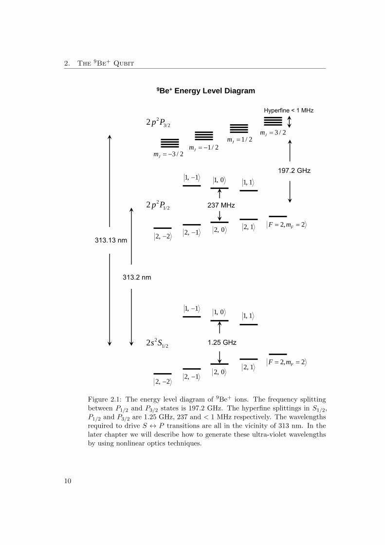
Figure 2.1: The energy level diagram of 9Be+ ions. The frequency splittingbetween P1/2 and P3/2 states is 197.2 GHz. The hyperfine splittings in S1/2,P1/2 and P3/2 are 1.25 GHz, 237 and < 1 MHz respectively. The wavelengthsrequired to drive S ↔ P transitions are all in the vicinity of 313 nm. In thelater chapter we will describe how to generate these ultra-violet wavelengthsby using nonlinear optics techniques.
10

2.2. Hyperfine Structure and Field-Independent Qubits
energy of any particular level is shifted according to the value of J , the excitedP state is split into two components, 2p 2P1/2 and 2p 2P3/2, with a splitting of197.2 GHz [Bollinger 85]. The 2s 2S1/2 ↔ 2p 2P1/2 and 2s 2S1/2 ↔ 2p 2P3/2
transitions are the components of a fine-structure doublet, and can be drivenvia electric dipole radiation in the vicinity of 313 nm. The excited state hasa lifetime of 8.2 ns, corresponding to a natural linewidth γ = 2π × 19.4 MHz.In spectroscopic notation, these states (2s 2S1/2, 2p 2P1/2 and 2p 2P3/2) willbe labeled as S1/2, P1/2 and P3/2 for simplicity.
The nuclear spin of the 9Be+ ion is I = 3/2 and thus it possesses hyperfinestructure, which is a result of the coupling of J with the nuclear angularmomentum I. This interaction leads to a splitting of the levels into stateswith a total angular momentum given by F = J + I. In the S1/2 state, thehyperfine splitting is 1.25 GHz [Wineland 83]; the hyperfine splittings in theexcited P1/2 state and P3/2 state are 237 MHz [Bollinger 85] and less than 1MHz respectively [Poulsen 75]. Each hyperfine manifold, for example F = 1manifold in S1/2 state, is degenerate at zero magnetic field. In the presence ofmagnetic fields, this degeneracy is broken by the Zeeman effect. For quantumcontrol, we use two Zeeman states in the S1/2 state as the quantum bit (qubit).In principle, we can choose any pair of levels for the qubit, but certain pairsare better for the quantum information processing than others since they havemuch longer coherence time. These will be discussed in Chapter 2.2.
2.2 Hyperfine Structure and Field-Independent Qubits
The hyperfine structure is a result of the coupling of J with the total nuclearangular momentum I. The Hamiltonian that describes the total system, in-cluding hyperfine interaction and the atomic interaction with the magneticfield, is
Htot = Hhfs +HB
Hhfs = hAhfsI ·JHB = µB(gSS + gLL + gII) ·B. (2.1)
For Hhfs, h is the Planck’s constant, and Ahfs is called the hyperfine constantand has an unit of frequency. The operators I and J are dimensionless. In ourdiscussions if we take the magnetic field to be along the z-direction, which isconsidered to be along the atomic quantization axis, HB can be written as
HB = µB(gSSz + gLLz + gIIz)Bz (2.2)
where µB is the Bohr magneton, and the quantities gS , gL, and gI are theelectron spin, electron orbital and nuclear g-factors, respectively. If the energyshift due to the magnetic field is small compared to the fine-structure splitting,
11

2. The 9Be+ Qubit
then J is a good quantum number and Eq. (2.2) becomes
HB = µB(gJJz + gIIz)Bz
Here, the Lande factor gJ is given by
gJ = gLJ(J + 1)− S(S + 1) + L(L+ 1)
2J(J + 1)+gS
J(J + 1) + S(S + 1)− L(L+ 1)
2J(J + 1)(2.3)
The Hhfs term described above only considers the interaction of the nuclearand electron magnetic dipoles. In general, the interaction between the nu-clear and electron angular momenta can be expanded in a multipole seriesso the higher-order corrections become quite involved, for example, the elec-tric quadrupole interaction, magnetic octupole interaction, etc [Woodgate 80].These interactions cause a shift of the hyperfine structure levels. In our case, tomore accurately determine the energy levels of P3/2 state we take the electric-quadrupole term into account. We should notice that this electric-quadrupoleinteraction is only applicable for the states with I, J > 1/2. Combining twoterms, the Hamiltonian for the hyperfine structure is
Hhfs = hAhfsI ·J
+hBhfs3(I ·J)2 + 3
2(I ·J)− I(I + 1)J(J + 1)
2I(2I − 1)J(2J − 1)(2.4)
where Bhfs is is the electric-quadrupole hyperfine constant.
Now we can compute the expectation values for the given total HamiltonianHtot = Hhfs + HB to obtain the energy levels as a function of applied mag-netic fields. When the Zeeman interaction is small compared to the hyperfineinteraction, the total angular momentum F = I+J and mF , which is the pro-jection of F on z-axis, are good quantum numbers to use because the Zeemaninteraction here is treated as a perturbation. In the opposite case where themagnetic field is very strong such that the Zeeman interaction dominates, theeigenstates are well described by the |I,mI ; J,mJ〉 basis (we will use |mI ,mJ〉for simplicity). However, for intermediate fields, where the Zeeman interac-tion neither perturbs nor dominates the hyperfine interaction, the system isin general difficult to calculate analytically. In general one must numericallydiagonalize the Hamiltonian Htot. There is an exception coming about inhyperfine structure when J = 1/2 (e.g. S1/2 and P1/2 states). In this case,the hyperfine Hamiltonian (Eq. (2.4)) is given only by the magnetic-dipoleterm and the energy levels can be solved analytically, which is so-called theBreit-Rabi formula [Woodgate 80]. I will focus on how to calculate the energylevels by diagonalizing the Hamiltonian so here I skip the detailed derivations
12

2.2. Hyperfine Structure and Field-Independent Qubits
B field (Gauss)0 50 100 150 200 250 300
E/h
(M
Hz)
-1000
-500
0
500
1000
1500
|2,-2i|2,-1i|2,0i|2,1i|2,2i|1,1i|1,0i|1,-1i
Figure 2.2: 9Be+ S1/2 (ground) state hyperfine structure in an exter-nal magnetic field. The parameters used in the calculation are Ahfs =−625.008837048 MHz, gL = 1, gS = 2.0023193043622, gJ obtained fromEq. (2.3), gI = gJ × 2.134779853 × 10⁻⁴, µB = 9.27400968 × 10⁻²⁴ J/Tesla[Yerokhin 08, Puchalski 09].
of the Breit-Rabi formula and only show the result [Woodgate 80]:
E|F,mF 〉 = − ∆Ehfs
2(2I + 1)+ gIµBmFB
±∆Ehfs
2
(1 +
4mFx
2I + 1+ x2
)1/2
(2.5)
where ∆Ehfs = Ahfs
(I + 1
2
)and x = µB(gJ−gI)B
∆Ehfs. For the beryllium ions, the
minus sign applies to the F = 1 manifold, the plus sign applied to F = 2manifold, and Ahfs can be found in [Yerokhin 08, Puchalski 09]. To avoid thediscontinuity in evaluating Eq. (2.5) the more direct formula
E|F,mF 〉 = − ∆Ehfs
2(2I + 1)+ gIµBmFB +
∆Ehfs
2(1 + x)
is used for the state mF = (I + 1/2). The physical picture behind the Breit-Rabi formula for quantum information processing is that it allows us to identifya pair of levels where the differential energy shift with respect to magnetic fieldvanishes to the first order. The main advantage of using such a transition asa qubit is that any small fluctuation in magnetic field does not influence thequbit frequency to the first order such that the qubit which stores the quantuminformation has a relatively long coherence time [Langer 05].
13

2. The 9Be+ Qubit
B field (Gauss)0 50 100 150 200 250 300
E/h
(M
Hz)
-300
-200
-100
0
100
200
300
|2,-2i|2,-1i|2,0i|2,1i|2,2i|1,1i|1,0i|1,-1i
Figure 2.3: 9Be+ P1/2 (excited) state hyperfine structure in an external mag-netic field. The hyperfine constant Ahfs used in the calculation is −117.919MHz [Yerokhin 08, Puchalski 09] and the rest are the same as for Fig. 2.2.
As mentioned above, the general way of calculating the energy levels of hyper-fine states is to numerically diagonalize the total Hamiltonian. In order to dothat, one needs to calculate the matrix elements for given computational basis.For convenience, here we only show the matrix elements using the Hamilto-nian in Eq. (2.1) for S1/2 and P1/2 states, and the matrix elements for theelectric-quadrupole interaction for the P3/2 state are given in Appendix A.Recalling the basic relations in quantum mechanics, we have
I ·J = IzJz + IxJx + IyJy
= IzJz +I+J− + I−J+
2
If now we choose the strong-field basis, the diagonal matrix elements are
〈mI ,mJ |Htot|mI ,mJ〉 = hAhfsmImJ + µB(gJmJ + gImI)B
and also the off-diagonal matrix elements are
〈mI + 1,mJ − 1|Htot|mI ,mJ〉 =
hAhfs
2
√(J −mJ + 1)(J +mJ)(I +mI + 1)(I −mI)
〈mI − 1,mJ + 1|Htot|mI ,mJ〉 =
hAhfs
2
√(J +mJ + 1)(J −mJ)(I −mI + 1)(I +mI)
14

2.2. Hyperfine Structure and Field-Independent Qubits
B field (Gauss)0 50 100 150 200 250 300
E/h
(M
Hz)
-1000
-500
0
500
1000
Figure 2.4: 9Be+ P3/2 (excited) state hyperfine structure in an external mag-netic field. The hyperfine splitting is already small in the low-field regime so itis not obvious that the levels are grouped according to the value of F , but theyare grouped according to mJ (from top to bottom: mJ = 3/2, 1/2, -1/2 and-3/2) as the magnetic field increases. The parameters used in the calculationare Ahfs = −1.015 MHz and Bhfs = −2.299 MHz [Yerokhin 08, Puchalski 09].
Using the eigenvalue solver in numerical software, we can easily obtain theenergy levels of hyperfine states in the presence of applied magnetic fields.
The energy levels for S1/2, P1/2 and P3/2 states as a function of magnetic fieldsare shown in Figs. 2.2, 2.3, and 2.4 respectively, ranging from the weak-field(Zeeman) regime through the strong-field regime. Although these spectrumare numerically solved by diagonalizing the Hamiltonian, for the states withJ = 1/2 the Breit-Rabi formula can be applied and produce the same results aswell. However, it does not apply to the P3/2 state in which the level structureis more complicated.
To determine which transition in S1/2 state is more desirable to use to per-form quantum information processing experiments, we differentiate each en-ergy level in Fig. 2.2 with respect to the B-field. Figure 2.5 shows the results.The first crossing point (at non-zero field) occurs at 119.4428 Gauss (G) forthe |S1/2, F = 2,mF = 0〉 ↔ |S1/2, F = 1,mF = 1〉 transition and the secondcrossing is at 119.6390 G for the |S1/2, F = 2,mF = 1〉 ↔ |S1/2, F = 1,mF =0〉 transition, showing these transitions are field-independent to the first or-der. The Ion Storage Group at NIST has demonstrated the qubit coherencetime up to 15 seconds [Langer 05] using a field-independent transition. Themagnetic field we use in our group is around 119.45 G.
15

2. The 9Be+ Qubit
B field (Gauss)0 50 100 150 200 250 300
@E
/@B
(ar
b. u
nit)
#1010
-1.5
-1
-0.5
0
0.5
1
1.5
|2,-2i|2,-1i|2,0i|2,1i|2,2i|1,1i|1,0i|1,-1i
Figure 2.5: Differential of energy ∂E/∂B versus B for the S1/2 ground stateof 9Be+ ions. Each crossing point is a first-order field-independent transitionthat occurs when ∂E/∂B is equal for both states. In our experiment, we canuse the first and the second field-independent transitions as the qubit states.
Here we define the bright state as |b〉 ≡∣∣S1/2, F = 2,mF = 2
⟩, which is
coupled to the state∣∣P3/2, F
′ = 3,m′F = 3⟩
and used for the qubit readout(see Chapter 2.4), and encode the two-level field-independent qubit (FIQ) as|↑〉 ≡
∣∣S1/2, F = 1,mF = 1⟩
and |↓〉 ≡∣∣S1/2, F = 2,mF = 0
⟩. If we work
with a standard field-dependent qubit (FDQ), those states are chosen as|↑〉 ≡
∣∣S1/2, F = 1,mF = 1⟩
and |b〉 = |↓〉 ≡∣∣S1/2, F = 2,mF = 2
⟩(see Fig.
2.6). More experimental characterizations will be discussed in Chapter 6.
2.3 Qubit Initialization
In 2000, David DiVincenzo summarized five requirements that any candidatequantum computer implementation must satisfy and two additional criteriafor quantum communication [DiVincenzo 00]. These are called DiVincenzocriteria. From previous discussions about the 9Be+ qubit transition, we havesatisfied the first DiVincenzo criteria, a scalable physical system with wellcharacterized qubits. I will introduce how we meet the second criteria, theability to initialize the state of the qubits to a well-defined state. We carryout this via optical pumping process. In the experiment, we use circularlypolarized σ+ laser light propagating along the direction of the magnetic fieldsince this is the only way of producing a purely σ+ light. The σ+ laser lightoptically pumps the internal state of the ion into |F = 2,mF = 2〉 state
16

2.3. Qubit Initialization
313.20 nm
197.2 GHz
69.08 76.39
86.69 102.80 MHz
76.25 86.55
B = 119.45 Gauss
600
MHz
1.2074958 GHz
20.09 MHz 23.14
28.24 39.93
23.09 28.19
224.6 MHz
260.8
MHz
Figure 2.6: The energy splittings of 9Be+ ions at B = 119.45 Gauss andthe required laser beams for cooling, detection and repumping. The brightstate used for qubit readout is |S1/2, F = 2,mF = 2〉. At this magneticfield the frequency splitting of the two-level field-independent qubit (FIQ) is1.2074958 GHz.
17

2. The 9Be+ Qubit
in the S1/2 ground state. The implementation consists of four laser beamsoverlapped in space with different frequencies at 313 nm. As shown in Fig.2.6, they are 1) The near-resonant “Blue Doppler” (BD) beam red detuned γ/2(γ = 2π × 19.4 MHz, the natural linewidth of the excited state as mentionedin Chapter 2.1) from the |S1/2, F = 2,mF = 2〉 ↔ |P3/2, F
′ = 3,m′F = 3〉cycling transition. 2) The “BD Detuned” (BDD) beam tuned 600 MHz to thered of the cycling transition. 3) The “Red Doppler F1” (RDF1) beam tunedslightly red of |S1/2, F = 1,mF = 1〉 ↔ |P1/2, F
′ = 2,m′F = 2〉, which pumpsthe population out of F = 1 manifold into |S1/2, F = 2,mF = 2〉 state. 4)The “Red Doppler F2” (RDF2) beam tuned slightly red or on resonance of|S1/2, F = 2,mF = 1〉 ↔ |P1/2, F
′ = 2,m′F = 2〉, which serves as repumpingfor the population not in |S1/2, F = 2,mF = 2〉 state.
The BDD beam is responsible for pre-cooling very hot ions while loading orafter collisions with thermal background gas. Because this beam is far detunedfrom resonance, it requires higher power than others in order to broaden thetransition. The parameters used in our experiments are the laser power ofapproximately few hundreds µW in ≈ 60 µm beam waist and the pulse lengthof 3.5 ms. We found that if the laser power of this beam is too high, the lineshape of the transition becomes too broad such that the cooling efficiencywould be decreased and the ions can not be crystalized. The BD beam servesthe Doppler cooling after the pre-cooling stage. Typically the time of Dopplercooling is around 700 µs in our case. The intensity of the Doppler beam is setto slightly below half of the saturation intensity (≈ 2.5 µW in 60 µm waistin our case). The saturation intensity is about 0.76 mW/mm2 for 9Be+ ion.The RDF1 and RDF2 beams assist optical pumping for F = 1 and F = 2manifolds when performing the resolved sideband cooling (see Chapter 6.4).The duration used for the optical pumping is around 5 µs with a certain opticalpower (see Chapter 6.3). It is worth noting that the high power BDD beamis also sufficient for optically pumping the F = 1 manifold even though it is≈ 400 MHz off-resonant from |S1/2, F = 1〉 ↔ |P3/2,mJ = 3/2〉 transitions.During the loading process, we could only use BD and BDD beams withoutRDF1 and RDF2 beams.
After the ion has been prepared in |S1/2, F = 2,mF = 2〉 state, there aretwo ways of preparing the ion in |S1/2, F = 1,mF = 1〉 state for driving thefield-independent transition. First, we can apply a π-pulse directly on the|S1/2, F = 2,mF = 2〉 ↔ |S1/2, F = 1,mF = 1〉 transition. Or we coulduse a combination of RDF2 beam with a Raman pulse that drives |S1/2, F =2,mF = 2〉 ↔ |S1/2, F = 2,mF = 1〉 transition such that the ion can bedissipatively pumped in |S1/2, F = 1,mF = 1〉 state.
For some experiments in which the ion needs to be cooled close to the motionalground state for the qubit initialization [Cirac 95, Meekhof 96], Raman side-band cooling is used. It is performed on |S1/2, F = 2,mF = 2〉 ↔ |S1/2, F =
18

2.3. Qubit Initialization
1,mF = 1〉 transition at 1017.9946 MHz, followed by a final repumping pro-cess to prepare the ion in |S1/2, F = 2,mF = 2〉 state. Sideband coolingtechnique can provide the ion in the motional ground state with > 99 % fi-delity [Wineland 98]. The experimental results are given in Chapter 6.4.
The infidelity of the ion’s internal state initialization (here we are interestedin |S1/2, F = 2,mF = 2〉 state preparation) arises from the impurity of po-larization of the RDF1 and RDF2 beams because this optical pumping is thefinal stage prior to any quantum operation. It is worth studying the prepara-tion error given some impurity in the polarization. We consider the opticalpumping rate out of |S1/2, F = 2,mF = 2〉 state due to the impure polar-ization in RDF2. The frequency of this beam is closest to the resonance of|S1/2, F = 2,mF = 2〉 ↔ |P1/2〉 transition so it can easily pump the populationaway from |S1/2, F = 2,mF = 2〉 state with non-σ+ light.
In the following analysis we assume that RDF2 beam has a small amount ofσ− and π polarization components. The optical pumping rate from the initialstate i to the final state f through a single excited state is
Γi→f =γ
2
s0
1 + s0 + 4δ2/γ2ci→f (2.6)
where γ is the natural linewidth, δ is the laser detuning from the excitedstate, and ci→j is the coupling coefficient between states i and j, which canbe calculated from the coefficients of eigenvector when solving the eigenvalueproblem of Eq. (2.1). s0 = I/Isat is the saturation parameter, where I is the
intensity of the laser beam and Isat = ~ω3γ12πc2
is the saturation intensity for whichω is 2π times the transition frequency and c is the speed of light. For an ionin |S1/2, F = 2,mF = 2〉, it can be excited to |P1/2, F
′ = 2,m′F = 2〉 state byabsorbing π polarized light. Then it will emit σ+ photons and decay to either|S1/2, F = 2,mF = 1〉 or |S1/2, F = 1,mF = 1〉 state. The total couplingcoefficient for this scattering event is
∑j ci→j = 2/9, which is the sum over a
product of the transition probabilities. The total coupling coefficient for thescattering through |P1/2, F
′ = 2,m′F = 1〉 state driven by σ− polarized lightis also 2/9. Both coupling coefficients are independent of the magnetic field.The optical pumping from |S1/2, F = 2,mF = 1〉 to |S1/2, F = 2,mF = 2〉state has a coupling coefficient of ∼ 1/18. Given an admixture of both π andσ− polarizations in the RDF2 beam, denoted with επ and εσ− , the opticalpumping rates from Eq. (2.6) are
Γσ− =γ
2
εσ−s0
1 + s0 + 4δ2σ−/γ
2
2
9
Γπ =γ
2
επs0
1 + s0 + 4δ2π/γ
2
2
9
The optical pumping rate with an ideal RDF2 beam (δ = 0) is
Γσ+ =γ
2
s0
1 + s0
1
18
19

2. The 9Be+ Qubit
Here we ignore the RDF2 beam acting on |S1/2, F = 1,mF = 1〉 ↔ |P1/2〉transition due to far off-resonance. Therefore the error in initialization (steadystate) can be evaluated as follows:
einit =Γπ
Γσ+
+Γσ−
Γσ+
=4(1 + s0)επ
1 + s0 + 4δ2π/γ
2+
4(1 + s0)εσ−
1 + s0 + 4δ2σ−/γ
2
For the 9Be+ ion working on the field-independent qubit at B = 119.45 G,δπ = 2π× 102.8 MHz and δσ− = 2π× 142.7 MHz. Assuming εσ− = επ = 0.1%and the saturation parameter s0 = 1, the error in initialization is einit ≈7.6× 10⁻⁵. The more general method to determine the initialization error isto solve the rate equation for all allowed transitions.
2.4 Qubit Readout
For trapped-ion experiments qubit read-out is performed by state-dependentfluorescence, which measures the projection of the state vector along a givenaxis. This technique was proposed by Dehmelt et al. [Dehmelt 75] and firstdemonstrated by Wineland et al. [Wineland 80]. It utilizes a closed transitionor so-called a cycling transition in the internal states of the ion. When excitinga cycling transition, the ion behaves like a two-level system. Performing thiskind of projective measurement collapses the ion’s wavefunction in either oneof its computational basis states. If one of the computational basis states isinvolved in the cycling transition, many photons can scatter without leavingthe transition and the fluorescence can be collected. In the opposite situation,if the ion’s wavefunction collapses to the basis state that does not participatein the cycling transition, only the background photons will be measured. Forthe 9Be+ ion, we use the BD beam, which has been mentioned in Chapter2.3, as the detection beam, but its frequency is tuned to be on resonanceof the |S1/2, F = 2,mF = 2〉 ↔ |P3/2, F
′ = 3,m′F = 3〉 or alternatively|P3/2,mI = 3/2,mJ = 3/2〉 cycling transition.
2.4.1 Readout Error - Dark to Bright State Leakage
The main source of the read-out error is the leakage of the qubits initially inthe dark state into the closed transition by off-resonantly coupling to other ex-cited states (other than the one in the closed transition) during measurement.When this happens, the ion in dark state has a possibility entering the closedtransition and then starts scattering at a high rate. For a multi-level atomicsystem like 9Be+ ions, the general treatment is to solve a rate equation forall allowed scattering paths such that the time evolution of the probability ofthe ion to be in any state can be calculated. The other advantage of the rate-equation treatment is that we are able to investigate how to improve dark to
20

2.4. Qubit Readout
bright state leakage by transferring the dark ion to the other hyperfine statewhich is even “darker”.
The population in each hyperfine ground state is represented by a vector v.For the 9Be+ ion, its length is 8. We define the rate matrix Γσ
+in which the
matrix elements Γσ+
i,j are the photon scattering rates from state |j〉 to state|i〉 and σ+ in the superscript means that we assume the polarization of thedetection beam is purely σ+. These non-zero matrix elements Γσ
+
i,j can becalculated using the Kramers-Heisenberg formula [Ozeri 05, Loudon 95]:
Γσ+
i,j =g2
4γ
∣∣∣∣∣∑m
a(m)i,j
∆m
∣∣∣∣∣2
(2.7)
where g = Eµ~ = γ
√s02 is the single-photon Rabi frequency (E is the elec-
tric field amplitude of the laser beam, and µ = |〈P3/2, F′ = 3,m′F = 3|d · σ+
|S1/2, F = 2,mF = 2〉| is the magnitude of the cycling transition electric-
dipole moment.), the coefficient a(m)i,j =
∑q〈i|d · σq|em〉〈em|d · σ+|j〉/µ2 is the
normalized transition strength from state |j〉 to state |i〉 through an interme-diate state |em〉 and here we sum over different polarizations q of the emittedlight, ∆m is the detuning of the detection beam from the |j〉 ↔ |em〉 transi-tion. We sum over m for all the excited states |em〉 in the P3/2 state. The P1/2
excited states are ignored in this case because they are ≈ 197 GHz away fromthe frequency of the detection beam. When ∆m is comparable to half of thepower broadened linewidth, Eq. (2.7) breaks down and we have to include animaginary damping term, iγ/2, in the detuning [Loudon 95]. By adding thisdamping term to the detuning, the Kramers-Heisenberg formula reproducesthe well-known total photon scattering rate in Eq. (2.6) for a two-level atom.
The time-dependent population transfer of each state is given by
∂vi∂t
=∑j
Γσ+
i,j vj − vi∑j
Γσ+
j,i (2.8)
that can be written as a matrix form:
∂v
∂t= Mσ+ ·v (2.9)
where Mσ+= Γσ
+ −D(1T ·Γσ+), 1 is a 8-by-1 matrix of ones, and D(x) is
a diagonal matrix with x in the diagonal elements. First, we solve Eq. (2.9)using the Laplace transform approach. After taking the Laplace transform, ityields
sV(s)− v(0) = Mσ+ ·V(s) (2.10)
where V(s) is the Laplace transform of v(t), v(0) is the initial condition, ands is the Laplace transform variable. Therefore, the solution can be easilyobtained
V(s) = −(Mσ+ − s1)−1v(0) (2.11)
21
2. The 9Be+ Qubit
where 1 is the identity matrix. For the given initial condition v(0), the time-domain solution v(t) can be calculated by taking the inverse Laplace transformof V(s). In the following, we show how to solve v(t).
We know from the control theory the term−(Mσ+−s1)−1 represents a transferfunction. The poles of the transfer function are the characteristic frequenciesof the system. Here we write a single term as a sum of partial fractions:[
(Mσ+ − s1)−1]i,j
=pi,j(s)
q(s)
=∑k
b(k)i,j
s+ ωk(2.12)
where q(s) =∏k(s+ωk) is the characteristic polynomial with roots −ωk (the
characteristic frequency), pi,j(s) is a polynomial in s, and
b(k)i,j = lim
s→−ωk
(s+ ωk)pi,j(s)
q(s)
=pi,j(ωk)∏
l 6=k(ωl − ωk)(2.13)
are constants assuming q(s) has no double roots that is the case for our detec-tion system. Therefore, the time-domain solution is given by:
vi,j(t) =
8∑k=1
b(k)i,j e−ωkt (2.14)
These are rate equation solutions for the time-dependent populations of eachstate. We are concerned with the probability of detecting the ion in the|F = 2,mF = 2〉 state at time t with the ion initially in other hyperfine states|j〉 at t = 0. It is given by
Pd→b(t) = vi=(2,2),j(t) =
8∑k=1
b(k)i=(2,2),je
−ωkt. (2.15)
A more general case would be including the polarization impurities in the de-tection beam. Ideally the polarization of the detection beam is purely σ+, butit might have εσ− admixture of σ− polarization and επ admixture of π polar-ization. We define new rate matrices Γσ
−and Γπ for σ− and π polarization
components respectively. Their matrix element and corresponding matrix M(Mπ and Mσ−) are given by
Γσ−i,j =
g2
4γ
∣∣∣∣∣∑m
c(m)i,j
∆m
∣∣∣∣∣2
, Γπi,j =g2
4γ
∣∣∣∣∣∑m
d(m)i,j
∆m
∣∣∣∣∣2
Mσ− = Γσ− −D(1T ·Γσ−), Mπ = Γπ −D(1T ·Γπ)
22

2.4. Qubit Readout
where c(m)i,j =
∑q〈i|d · σq|em〉〈em|d · σ−|j〉/µ2 and d
(m)i,j =
∑q〈i|d · σq|em〉〈em|
d · π|j〉/µ2. Because we solve a differential equation with the same form asEq. (2.9), we have to find a new matrix M, which now is the sum over all thepolarization components and can be defined as
M =1
(1− εσ− − επ)2 + ε2σ− + ε2π
[(1− εσ− − επ)2Mσ+
+ ε2σ−Mσ− + ε2πMπ]
(2.16)Following the same procedures described above to solve ∂v
∂t = M ·v for giveninitial conditions, the time-dependent populations of each state can be calcu-lated.
We can now study the read-out error a bit further by looking at the distributionof photon counts for the dark state ion. This information is useful if we aregoing to optimize the qubit readout fidelity. We have seen from Eq. (2.15) thatthe probability of scattering from a dark state into the bright state is the sumover exponential terms. Therefore for a qubit initially in the dark state, weexpect the probability distribution of collected photons to be a convolution ofPoisson and exponential distributions [King 99]. We introduce a general waywhich can apply to different cases based on the derivations given by Acton etal. [Acton 05] and Langer [Langer 06].
Using Eq. (2.15), the probability that the ion leaves the dark state to thebright state between t and t+ dt is given by
|Pd→b(t)dt| =8∑
k=1
b(k)i=(2,2),jωke
−ωktdt (2.17)
When the dark ion goes into the bright state at time t, the collected photonswill obey Poisson statistics with a mean given by
λ(t) = λbg + (1− t
τD)λ0 (2.18)
where λ0 = γcτD is the mean of the bright photon distribution (without back-ground), and λbg = rbgλ0 is the mean of the background photon distribution.τD is the detection time, γc = ζ γ2
s01+s0
is the rate of collecting photons in theclosed transition in which ζ is the total detection efficiency, and rbg is the rateof collecting background photons normalized by γc. We desire to transformfrom a probability distribution Pd→b(t)dt to a probability distribution of Pois-sonian means, g(λ)dλ. We use Eq. (2.18) to get t(λ) and then substitute intoEq. (2.17). This yields the probability that the collected photons from a darkion produces a Poisson distribution with mean λ:
g(λ)dλ =
−∑
k b(k)i=(2,2),j
ωkγce−ωkγc
(λbg+λ0−λ)dλ, λbg < λ ≤ λbg + λ0
1−∑
k b(k)i=(2,2),je
−ωkτD , λ = λbg(2.19)
23

2. The 9Be+ Qubit
Here when λ = λbg, it means that the dark ion never enters the bright state,and the probability that the dark ion behaves like Poisson statistics with meanλbg is 1− Pd→b(τD).
Therefore, the probability of detecting n photons when starting in the darkstate is simply the convolution of the density of means g(λ) with the Poisson
distribution P (n|λ) = e−λλn
n! :
pdark(n|j) =
(1−
∑k
b(k)i=(2,2),je
−ωkτD)P (n|λbg)−∫ λbg+λ0
λbg
e−λλn
n!
∑k
b(k)i=(2,2),j
ωkγce−ωkγc
(λbg+λ0−λ)dλ
= P (n|λbg)−∑k
b(k)i=(2,2),je
−ωkτD(P (n|λbg) +
ωke−ωkγcλbg
γcn!
∫ λbg+λ0
λbg
eωkλ/γce−λλndλ
)We can rewrite the above equation in terms of incomplete Gamma functionas follows:
pdark(n|j) = P (n|rbgγcτD)−∑k
b(k)i=(2,2),je
−ωkτD(P (n|rbgγcτD) +
ωkγnc e−ωkτDrbg
(γc − ωk)n+1
[P(n+ 1, (γc − ωk)(1 + rbg)τD)
− P(n+ 1, (γc − ωk)rbgτD])
(2.20)
where P(a, x) ≡ 1(a−1)!
∫ x0 e−yya−1dy is the incomplete Gamma function nor-
malized such that P(a,∞) = 1.
2.4.2 Readout Error - Bright to Dark State Pumping
Similarly, the ion in the bright state can be optically pumped into a dark statedue to imperfect detection beam polarization. This will cause the measure-ment error. If the polarization of the detection beam has a small fraction of π(σ−) polarization, the bright state (|S1/2, F = 2,mF = 2〉) can off-resonantlycouple to the |P3/2,mJ = 1/2〉 (|P3/2,mJ = −1/2〉) state with the detuningof ≈ 225 (450) MHz for the magnetic we use (see Fig. 2.6) and then decayto a dark state. In the experiment, the detection beam is aligned parallel tothe magnetic field in order to have purely σ+ light. However, if the opticalalignment is not perfect, the polarization that the ion sees may contain π andσ− components. We can reduce imperfect polarizations by tilting and rotat-ing the quarter-wave plate in front of the vacuum chamber by minimizing the
24

2.4. Qubit Readout
amount of dark photon counts on the histogram for the ion prepared in thebright state.
This optical pumping process from the bright state to a dark state can betheoretically analyzed using the methods similar to that in the previous section.Here we are interested in the time-dependent population change in the |F =
2,mF = 2〉 state, which is Pb(t) = vi=(2,2),j=(2,2)(t) =∑8
k=1 b(k)i=(2,2),j=(2,2)e
−ωkt
from Eq. (2.15). The probability density for the ion in the bright state betweent and t+ dt is given by
|Pb(t)dt| =8∑
k=1
b(k)i=(2,2),j=(2,2)ωke
−ωktdt (2.21)
If the ion leaves the bright state at time t, the collected photon will exhibitPoisson statistics with a mean given by
λ(t) = rbgγcτD + γct (2.22)
The probability that the collected photons from a bright ion produces a Pois-son distribution with mean λ:
g(λ)dλ =
∑k b
(k)i=(2,2),j=(2,2)
ωkγceωkγc
(λbg−λ)dλ, λbg ≤ λ < λbg + λ0∑
k b(k)i=(2,2),j=(2,2)e
−ωkτD , λ = λbg + λ0
(2.23)
Here when λ = λbg + λ0, the bright ion never leaves the bright state, and theprobability that the bright ion follows Poisson statistics is Pb(t).
As before, the overall photon probability distribution will be a convolution ofPoisson and exponential distributions. However the process is now reversedthat after some time the bright ion is pumped into a dark state and emits nomore photons. The probability of detecting n photons when starting in thebright state is:
pbright(n) =∑k
b(k)i=(2,2),j=(2,2)e
−ωkτDP (n|(1 + rbg)γcτD) +
∑k
b(k)i=(2,2),j=(2,2)
ωkγnc e
ωkτDrbg
(γc + ωk)n+1
[P(n+ 1, (γc + ωk)(1 + rbg)τD)
− P(n+ 1, (γc + ωk)rbgτD
](2.24)
where the first term is the Poisson distribution from never leaving the cyclingtransition and the second term is the the distribution from pumping to a darkstate.
2.4.3 Simulation Results and Discussion
Here we have provided a theoretical study about the qubit readout errors. InChapter 6, we will give the discussions for the simulations, accompanying withexperimental results.
25

2. The 9Be+ Qubit
|1
| 2
| 3
br
r
b
Figure 2.7: Energy level diagram for two-photon stimulated Raman transi-tions. The “blue” Raman beam couples levels |3〉 and |1〉 with a single-photondetuning ∆b = ωb − ω31. The “red” Raman beam couples levels |3〉 and |2〉with a single-photon detuning ∆r = ωr − ω32. The two-photon detuning isdefined as δ = ∆b −∆r.
2.5 Stimulated Raman Transitions
Since we encode the qubit into two of the hyperfine ground states, the qubit ma-nipulations and coherent operations are realized by two-photon stimulated Ra-man transitions. We consider the energy level structure in the Λ-configuration,as shown in Fig. 2.7, where two ground states, | ↓〉 ≡ |1〉 and | ↑〉 ≡ |2〉, arecoupled to an excited state |e〉 ≡ |3〉 by two laser fields. These states have en-ergies ~ω1, ~ω2, and ~ω3 respectively corresponding to an atomic HamiltonianH0 = ~ω1|1〉〈1|+~ω2|2〉〈2|+~ω3|3〉〈3|. The |1〉 ↔ |3〉 and |2〉 ↔ |3〉 transitionsare dipole allowed transitions. The two monochromatically laser fields are la-beled with Ei = εiEicos(ki · r − ωit + φi) for i ∈ b, r. Here, Ei and εi arethe amplitude and the polarization of the electric field, ki is the wave vector,r is the position of the ion, and ωi and φi are the frequency and the phaseof the laser respectively. The goal is to show that under certain conditions,the internal states and motional states of the ion can be coherently controlledbetween states |1〉 and |2〉 without significantly populating the excited state.This is effectively mapped to a two-level system.
The electric field interacts with the atomic dipole, given by d = er, whichcan be expressed in terms of the atomic eigenstates and the dipole matrixelements µa,b = 〈a|d|b〉:
d = µ1,3|1〉〈3|+ µ3,1|3〉〈1|+ µ2,3|2〉〈3|+ µ3,2|3〉〈2| (2.25)
We have used the property that states |1〉, |2〉 and |3〉 have opposite paritysuch that 〈1|d|1〉 = 〈2|d|2〉 = 〈3|d|3〉 = 0. The dynamics of the system is
26

2.5. Stimulated Raman Transitions
governed by the full Hamiltonian for the three-level atom and classical fields:
H = ~ω21|2〉〈2|+ ~ω31|3〉〈3|+ d ·∑i
Ei
= ~ω21|2〉〈2|+ ~ω31|3〉〈3|+
~g∗b |1〉〈3|1
2
(ei(kb · r−ωbt+φb) + e−i(kb · r−ωbt+φb)
)+
~gb|3〉〈1|1
2
(ei(kb · r−ωbt+φb) + e−i(kb · r−ωbt+φb)
)+
~g∗r |2〉〈3|1
2
(ei(kr · r−ωrt+φr) + e−i(kr · r−ωrt+φr)
)+
~gr|3〉〈2|1
2
(ei(kr · r−ωrt+φr) + e−i(kr · r−ωrt+φr)
)(2.26)
where we define the single-photon Rabi frequencies as gb ≡ Eb〈3|d · εb|1〉~ and
gr ≡ Er〈3|d · εr|2〉~ , and define ω21 = ω2 − ω1 and ω31 = ω3 − ω1 by setting
the energy of |1〉 state to zero. We then transform the Hamiltonian to an
appropriate rotating frame via the transformation Hrot = UHU † − i~U dU†
dt
with the unitary operator U = ei((ωb−ωr)|2〉〈2|+ωb|3〉〈3|)t. Equation (2.26) can bewritten as
Hrot = −~∆|3〉〈3| − ~δ|2〉〈2|+
~g∗b2|1〉〈3|e−i(kb · r+φb) + ~
gb2|3〉〈1|ei(kb · r+φb) +
~g∗r2|2〉〈3|e−i(kr · r+φr) + ~
gr2|3〉〈2|ei(kr · r+φr) (2.27)
where ∆ = ∆b = ωb−ω31 the single-photon detuning, δ = ∆b−∆r is the two-photon detuning in which ∆r = ωr−ω32, and we have made the rotating-waveapproximation (RWA) in which the high-frequency oscillating terms (e±i2ωbt
and e±i2ωrt) are omitted. The general form of the state
|ψ〉 = c1(t)|1〉+ c2(t)|2〉+ c3(t)|3〉
obeys the Schrodinger equation
i~d
dt|ψ〉 = Hrot|ψ〉
yielding equations of motion for the population amplitudes as follows:
ic1 =g∗b2c3e−i(kb · r+φb) (2.28)
ic2 = −δc2 +g∗r2c3e−i(kr · r+φr) (2.29)
ic3 = −∆c3 +gb2c1e
i(kb · r+φb) +gr2c2e
i(kr · r+φr) (2.30)
27

2. The 9Be+ Qubit
This Λ-system has a simple solution for large single-photon detuning ∆ gb, gr, δ. Since ∆ is much larger than other time scales in the problem, tothe lowest order in gb,r/∆ the excited state amplitude will be constant, with
c3 =gbc1e
i(kb · r+φb) + grc2ei(kr · r+φr)
2∆(2.31)
Substituting c3 back to Eqs. (2.28) and (2.29), we obtain the evolution of theprobability amplitude for the two ground states
ic1 =|gb|2
4∆c1 +
g∗bgre−i((kb−kr) · r+φb−φr)
4∆c2 (2.32)
ic2 =gbg∗rei((kb−kr) · r+φb−φr)
4∆c1 + (−δ +
|gr|2
4∆)c2 (2.33)
These equations are equivalent to the equations of motion for a two levelsystem with a Rabi frequency
Ω =gbg∗r
2∆ei((kb−kr) · r+φb−φr), (2.34)
which is also called effective Rabi frequency for the Raman transition, Ramanfrequency or two-photon Rabi frequency, and AC Stark shifts
δsb =|gb|2
4∆(2.35)
δsr =|gr|2
4∆(2.36)
induced from the detuned laser fields. After rewriting Eqs. (2.32) and (2.33),we get
ic1 = δsbc1 +Ω∗
2c2 (2.37)
ic2 =Ω
2c1 + (−δ + δsr)c2 (2.38)
The above equations of motion can be viewed as resulting from the Hamilto-nian
H = ~δsb|1〉〈1|+ ~(−δ + δsr)|2〉〈2|+~2
(Ω|2〉〈1|+ Ω∗|1〉〈2|) (2.39)
Basically the AC Stark shift terms can be removed by re-defining the energylevel reference. To calculate the dynamics of a standard two-level system,again we choose the zero energy level in the middle of two states and introducea detuning like δ′ = δ − δsr + δsb such that Eq. (2.39) can be rewritten as
H = −~δ′|2〉〈2|+ ~2
(Ω|2〉〈1|+ Ω∗|1〉〈2|) (2.40)
28

2.5. Stimulated Raman Transitions
Using the unitary operator U = e−iδ′|2〉〈2|t and transferring Eq. (2.40) to a
new rotating frame, the resulting Hamiltonian is
HI =~2
Ω0
(|2〉〈1|ei(∆k · r+∆φ)e−iδ
′t + |1〉〈2|e−i(∆k · r+∆φ)eiδ′t)
(2.41)
where Ω0 = |Ω| = gbg∗r
2∆ , ∆k = kb−kr, and ∆φ = φb−φr. This form is like theHamiltonian for a two-level system in the interaction picture. The dynamicsof the system is the well-known Rabi oscillations, where the time evolution ofthe population of the state behaves like a sinusoidal function at a rate givenby the Rabi frequency Ω0.
2.5.1 Multiple Excited States
The techniques for treating the three-level system are also applicable to thecase in which the ground states are coupled to multiple excited states. Essen-tially this always happens in real atoms or ions. To illustrate how to extendthe three-level calculation to multiple excited states, we consider an ion withtwo ground states (qubit states) as before and many excited states |e〉. Eachexcited state is coupled to |1〉 by the field Eb and coupled to |2〉 by the fieldEr. Equation (2.27) is modified to be
Hrot = −~∑m
∆m|em〉〈em| − ~δ|2〉〈2|+
~∑m
g∗b,em2|1〉〈em|e−i(kb · r+φb) + ~
∑m
gb,em2|em〉〈1|ei(kb · r+φb) +
~∑m
g∗r,em2|2〉〈em|e−i(kr · r+φr) + ~
∑m
gr,em2|em〉〈2|ei(kr · r+φr)(2.42)
The derivation is basically the same as before, except for the summation ofthe excited states and the dependence of the detunings from different excitedstate. Following the same procedure above, we find that the Raman Rabifrequency and AC Stark shifts are now given by
|Ω| = Ω0 =∑m
gb,emg∗r,em
2∆
=EbEr2~2
∑m
〈2|d · εr|em〉〈em|d · εb|1〉∆m
(2.43)
and
δsb =∑m
|gb,em |2
4∆m=E2b
4~2
∑m
|〈em|d · εb|1〉|2
∆m(2.44)
δsr =∑m
|gr,em |2
4∆m=E2r
4~2
∑m
|〈em|d · εr|2〉|2
∆m(2.45)
29

2. The 9Be+ Qubit
2.5.2 Ion’s Motion
In the previous section we have showed that we can coherently drive the popu-lations between two ground internal states of an ion by using two laser beamsdetuned from an excited state with a beatnote frequency close to the energylevel splitting of the qubit. For the other degree of freedom, because the ion isstrongly confined in a harmonic potential, its motion is quantized. Therefore,we can take the motional effects into account by adding the harmonic oscillatorHamiltonian Hosc = ~ωza†a to the base Hamiltonian H0, where we only con-sider ωz, the vibrational frequency along the z axis. The motional-dependentterm in Eq. (2.41) needs to be modified as ∆k · r→ ∆kz z = η(a†+ a) in whichwe only consider the motion in z-axis. Here η = ∆kzz0 is the Lamb-Dicke pa-
rameter and z0 =√
~2mωz
is the root mean squared extent of the oscillator
ground state wavepacket.
Applying the transformation e−iHosct/~HIeiHosct/~ to Eq. (2.41) and making
use of Baker Campbell Hausdorff formula, the interaction Hamiltonian in theinteraction picture is
H ′I =~2
Ω0 |↑〉 〈↓| expiη(ae−iωzt + a†eiωzt)ei(φ−δ′t) + h.c. (2.46)
where ‘h.c.’ means the hermitian conjugate of the first term, and ∆φ, |1〉and |2〉 in Eq. (2.41) have been replaced with φ, |↓〉, and |↑〉 respectively.Depending on the laser detuning δ′, the interaction Hamiltonian couples ion’sinternal and motional states (|↓, n〉 and |↑, n+ s〉, where s is an integer and|n〉 are the eigenstates of the harmonic oscillator).
Rabi Frequencies
With the closure relation, an arbitrary operator O can be expressed in theform O =
∑n,n′ |n′〉〈n′|O|n〉〈n| such that Eq. (2.46) can be written as
H ′I =∑n,n+s
~2
Ω0〈n+ s|eiη(ae−iωzt+a†eiωzt)|n〉| ↑, n+ s〉〈↓, n|ei(φ−δ′t) + h.c.
=∑n,n+s
~2
Ω0〈n+ s|D(iηeiωzt)|n〉| ↑, n+ s〉〈↓, n|ei(φ−δ′t) + h.c. (2.47)
where D(α) = eαa†−α∗a denotes the displacement operator. We then deter-
mine the matrix elements of displacement operator. For n+ s ≥ n (s ≥ 0), wecan show the result in the following by applying the Baker-Campbell-Hausdorffformula and basic properties of the annihilation operator:
〈n+ s|D(α)|n〉 = e−|α|2/2〈n+ s|eαa†eα∗a|n〉
= e−|α|2/2αs
√n!
(n+ s)!Lsn(|α|2),
30

2.5. Stimulated Raman Transitions
where Lsn(|α|2) are the generalized Laguerre polynomials. Analogously, forn+ s ≤ n (s ≤ 0), we obtain
〈n+ s|D(α)|n〉 = e−|α|2/2(−α∗)−s
√(n+ s)!
n!L−sn+s(|α|
2),
At the end, it turns out that Eq. (2.47) is
H ′I =∑n,n+s
~2
Ωn+s,ni|s|| ↑, n+ s〉〈↓, n|ei(sωz−δ′t+φ) + h.c. (2.48)
in which
Ωn+s,n = Ω0e−η2/2η|s|
√n<!
n>!L|s|n<(η2) (2.49)
where n< (n>) is the lesser (greater) of n+ s and n [Wineland 98]. The timeevolution for the general state
|Ψ(t)〉 =∞∑n=0
c↓,n(t)| ↓, n〉+ c↑,n(t)| ↑, n〉 (2.50)
can be calculated by solving the Schrodinger equation with the Laplace trans-form method, yielding the solution[
c↑,n+s(t)c↓,n(t)
]= U sn
[c↑,n+s(0)c↓,n(0)
](2.51)
with
U sn =
[e−i(δs/2)t
[cos(X2 t)
+ i δsX sin(X2 t)]−iΩn+s,n
X ei(φ+|s|π/2−δst/2)sin(X2 t)
−iΩn+s,n
X e−i(φ+|s|π/2−δst/2)sin(X2 t)
ei(δs/2)t[cos(X2 t)− i δsX sin
(X2 t)] ]
(2.52)
where δs = δ′−sωz and X =√δ2s + Ω2
n+s,n. This time-domain solution shows
the generalized form of Rabi flopping between states | ↓, n〉 and | ↑, n+ s〉.
Lamb-Dicke Approximation
Once the ions are cold, experiments are carried out in the Lamb-Dicke (LD)regime where the extension of the ion’s wavefunction is much smaller than1/k. When the condition for the LD regime is satisfied, the exponent in Eq.(2.46) can be expanded to the first order in η, resulting in
H ′I,LD =~2
Ω0σ+1 + iη(ae−iωzt + a†eiωzt)ei(φ−δ′t) + h.c. (2.53)
where σ+ ≡ |↑〉 〈↓| and σ− ≡ |↓〉 〈↑| are the spin flip operators. There are threedifferent types of coupling forming the basic coherent operations for all the
31

2. The 9Be+ Qubit
Ion motion Internal states
Coupled system: ladder structure
Figure 2.8: A two-level system coupled to a harmonic oscillator results in theladder structure. Three types of couplings (carrier, blue sideband, and redsideband drives) are shown.
quantum information and quantum computation experiments using trappedions. 1) When δ′ = 0, the Hamiltonian is simplified to
Hcar =~2
Ω0
(σ+e
iφ + σ−e−iφ)
(2.54)
which is called the carrier Hamiltonian and only drives the transition betweentwo internal states without coupling to the ion’s motion. 2) When δ′ = −ωz,the Hamiltonian becomes
Hrsb =~2
Ω0η(aσ+e
iφ + a†σ−e−iφ)
(2.55)
This Hamiltonian is called the first red sideband Hamiltonian and equivalentto the famous Jaynes-Cummings Hamiltonian in quantum optics. It drives| ↓, n〉 ↔ | ↑, n − 1〉 transition with Rabi frequency Ωn−1,n = Ω0
√nη. 3)
When δ′ = ωz, which is the counterpart of the second type of coupling, theHamiltonian is simplified to
Hrsb =~2
Ω0η(a†σ+e
iφ + aσ−e−iφ)
(2.56)
This is the first blue sideband Hamiltonian or called anti-Jaynes-CummingsHamiltonian, coupling | ↓, n〉 and | ↑, n + 1〉 with Rabi frequency Ωn+1,n =
32

2.6. Quantum Gates
Ω0
√n+ 1η. Figure 2.8 shows the ladder structure of a two-level system cou-
pled to a harmonic oscillator and the three types of couplings are indicated.With proper use or certain combination of these coherent operations, one canperform a variety of experiments with trapped ions.
2.6 Quantum Gates
Although we haven’t realized the two-qubit gate operations in our experimentsyet, in this Section I will introduce the theoretical background of single-qubitand two-qubit gates using 9Be+ ions. The reasons are that we have performedsome theoretical studies for the gate error analysis (see next Section) as wellas set up the apparatus that can be used for implementing the two-qubit gates(see Chapter 5).
2.6.1 Single-Qubit Quantum Gates
The single-qubit gate operations are implemented using the stimulated Ramantransition described previously with two co-propagating Raman beams. Theadvantage of the co-propagating Raman beams is that the difference of two kvectors is close to zero, (kb − kr) ≈ 0, which means this action is insensitiveto the ion’s motion (∆k · r is extremely small.). For the resonant carriertransitions (δ′ = 0 and s = 0), Eq. (2.51) is simplified to[
c↑,n(t)c↓,n(t)
]= R(θ, φ)
[c↑,n(0)c↓,n(0)
](2.57)
with
R(θ, φ) =
[cos(θ2
)−ieiφsin
(θ2
)−ie−iφsin
(θ2
)cos(θ2
) ](2.58)
where θ ≡ Ω0t and φ = ∆φ = φb − φr in the case of stimulated Ramantransitions. The rotation matrices R(π, φ) and R(π/2, φ) are a π-pulse and aπ/2-pulse respectively with a phase φ. The θ is varied by the laser pulse dura-tion for a given Rabi frequency (laser intensity). The phase can be controlledby the differential phase between the two Raman beams generated from stablemicrowave sources. With suitable settings, we are able to perform arbitraryrotations about any axis on the Bloch sphere.
2.6.2 Two-Qubit Quantum Gates
The final element of the universal gate set is the two-ion entangling gate. Sincewe encode the quantum information onto the ion’s spin states, an entanglingoperation is completed between two ions’ spin states. The efficient way toobtain the entanglement of two ions is through their collective motion.
33

2. The 9Be+ Qubit
In this Section, I will mainly explain two gate operations using a state de-pendent force (SDF) as well as discuss some experimental issues. Both gatesbasically work in the same way but in different computational basis. Thefirst one is the conditional phase gate in z basis of the spin states, namelythe geometric phase gate (Z-phase gate or σz gate) [Leibfried 03b, Roos 08];the second is called Mølmer-Sørensen gate (MS gate or σφ gate) [Mølmer 99,Benhelm 08a, Roos 08] operating in the basis other than z. The main ideais that the force acting on the two ions creates internal-state dependent dis-placement in the position-momentum (x−p) phase space. After completion ofthe force application, the trajectory of particular two-qubit states is a closedloop in the phase space while acquiring a state-dependent geometric phaseproportional to the area of the loop. This geometric phase can lead to anentanglement between spin states.
Geometric Phase Gate
For 9Be+ ions, the two-qubit operations are also performed using stimulatedRaman transitions. Here the geometric phase gate uses a pair of non coprop-agating Raman beams illuminating on two ions. The frequency differencebetween the two Raman beams δ = ωa − ωb is set close to one of the vibra-tional frequencies of the ion chain. The fields couple each of the spin statesvia an the excited state with a large detuning ∆ compared to the qubit split-ting frequency ω↑↓ (See Fig. 2.9). With this arrangement, states |↓〉 and |↑〉are not coupled by the laser beams because the beatnote frequency δ is faraway from the qubit transition frequency ω↑↓. Thus we can think that tran-sitions |↓〉 ↔ |e〉 and |↑〉 ↔ |e〉 are two independent two-level systems. TheHamiltonian for one of the two-level systems can be written as
H = ~ωe↓ |e〉 〈e|+~g∗a2|↓〉 〈e|
(ei(ka · r−ωat+φa) + e−i(ka · r−ωat+φa)
)+
~ga2|e〉 〈↓|
(ei(ka · r−ωat+φa) + e−i(kb · r−ωat+φa)
)+
~g∗b2|↓〉 〈e|
(ei(kb · r−ωbt+φb) + e−i(kb · r−ωbt+φb)
)+
~gb2|e〉 〈↓|
(ei(kb · r−ωbt+φb) + e−i(kb · r−ωbt+φb)
)(2.59)
Applying the RWA and adiabatic elimination of the excited state, the Hamil-tonian in an appropriate rotating frame is
HI = ~[δs↓ +
Ω↓2
(ei(∆k · r−δt+∆φ) + h.c.
)]|↓〉 〈↓| (2.60)
where ∆k = ka−kb, ∆φ = φa−φb, δs↓ = |ga|2+|gb|24∆ is the time-averaged Stark
shift on the level |↓〉 and Ω↓ =gag∗b2∆ is the time-varying Stark shift due to the
34
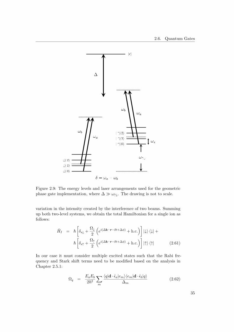
2.6. Quantum Gates
Figure 2.9: The energy levels and laser arrangements used for the geometricphase gate implementation, where ∆ ω↑↓. The drawing is not to scale.
variation in the intensity created by the interference of two beams. Summingup both two-level systems, we obtain the total Hamiltonian for a single ion asfollows:
HI = ~[δs↓ +
Ω↓2
(ei(∆k · r−δt+∆φ) + h.c.
)]|↓〉 〈↓|+
~[δs↑ +
Ω↑2
(ei(∆k · r−δt+∆φ) + h.c.
)]|↑〉 〈↑| (2.61)
In our case it must consider multiple excited states such that the Rabi fre-quency and Stark shift terms need to be modified based on the analysis inChapter 2.5.1:
Ωq =EaEb2~2
∑m
〈q|d · εa|em〉〈em|d · εb|q〉∆m
(2.62)
35

2. The 9Be+ Qubit
and
δsq =∑j=a,b
E2j
4~2
∑m
|〈em|d · εj |q〉|2
∆m(2.63)
where q ∈ ↓, ↑. By carefully choosing the polarizations for the two Ra-man beams, the time-averaged Stark shifts (δs↓ and δs↑) can be made equalsuch that there is no net time-averaged Stark shift between states |↓〉 and |↑〉[Wineland 03, Leibfried 03b]. If one makes Ω↓ 6= Ω↑, a differential Stark shiftwill result in a differential force between the two spin states. In the exper-iment, the goal is to make |Ω↓ − Ω↑| as large as possible. In the followingdiscussions, we will ignore δs↓ and δs↑ terms because both do not affect thefinal result.
Using the same mathematical treatments in Chapter 2.5.2 for ion’s motion,we find that the interaction Hamiltonian (Eq. (2.61)) with Lamb-Dicke ap-proximation is
H ′I,LD =∑q=↑,↓
~2
Ωq1 + iη(ae−iωzt + a†eiωzt)ei(∆φ−δt)|q〉〈q|+ h.c.
After we simplify the equation and skip the fast oscillating terms by RWA,the remaining term is
H ′I,LD =∑q=↑,↓
~2iηΩq
(a†ei[(ωz−δ)t+∆φ] − ae−i[(ωz−δ)t+∆φ]
)|q〉〈q| (2.64)
When N ions are trapped in the same potential, there are N vibrational modesin each principal axis. For two ions, the two modes in the axial direction are thecenter-of-mass (COM) mode where two ions oscillate in phase and the stretchmode where the ions oscillate out of phase. Application of the gate operationto two ions on the stretch mode (the motional heating for this mode is lower[Leibfried 03b]) can be analyzed by summing over the individual Hamiltonian(Eq. (2.64)):
HI = (+1)H′(1)I,LD + (−1)H
′(2)I,LD
=∑j=1,2
∑q=↑,↓
~2iη(−1)j−1Ωqj
(a†ei[(ωz−δ)t+φj ] − ae−i[(ωz−δ)t+φj ]
)|qj〉〈qj |
=∑q=↑,↓
(Fq1,q2zs
2a†ei(ωz−δ)t +
F ∗q1,q2zs
2ae−i(ωz−δ)t
)|q1q2〉〈q1q2| (2.65)
where Fq1,q2zs = i~η(Ωq1eiφ1 − Ωq2e
iφ2) in which zs is the root mean squaredextent of the ground state wavepacket for the stretch mode and Fq1,q2 is thespin-state-dependent force on both ions associated with the computational
36

2.6. Quantum Gates
basis |q1q2〉. For Eq. (2.65) it is important to notice that 1) the motionalmode is common to both ions; 2) The phase φj = (∆k · z)zj + ∆φ is differentfor two ions because they are in different locations (zj denotes the locationof the jth ion along the z-axis). We can see that the optical phase differenceφ1 − φ2 determines the phase difference between the forces. However if twoions are spaced by an integer multiple of the effective optical wavelength λeff =2π/|∆k| ≈ 215 nm, they experience the same phase of the optical field, i.e.φ1 = φ2. The differential force would be determined by the the magnitudeand the sign of Ωq1 and Ωq2. This implies that when two spin states are thesame there is no differential force. On the other hand, when the spin states areanti-aligned each ion would experience different forces because Ω↓1 6= Ω↑2 andΩ↓2 6= Ω↑1; 3) Once the ion-ion separation is adjusted to fulfill the conditionmentioned above, then the sign of the individual Hamiltonian depends onwhich vibrational mode is driven. The sign of the Hamiltonian for the secondion is negative due to the use of the stretch mode.
We desire to calculate the time evolution for HI . The matrix elements Hq1,q2 =Fq1,q2zs
2 a†ei(ωz−δ)t+F ∗q1,q2zs
2 ae−i(ωz−δ)t are the motional parts corresponding toeach computational eigenstate and are only located in the diagonal of theHamiltonian matrix. Hq1,q2 does not commute with itself at different times.However for a very short time interval ∆t the evolution of a wavefunction canstill be written as |Ψ(t + ∆t)〉 = exp
(− i
~Hq1,q2∆t)|Ψ(t)〉. It can be found
that
exp
(− i~Hq1,q2∆t
)= exp
(∆αa† −∆α∗a
)= D(∆α)
where D(α) is the displacement operator and the small displacements ∆α =− i
2~Fq1,q2zsei(ωz−δ)t∆t for which the real and the imaginary parts can be un-
derstood as its position and momentum parts in phase space. By repeatedlyusing the relation D(α)D(β) = D(α + β)exp [iIm(αβ∗)] [Walls 94], we areable to add all the infinitesimal displacements to construct the time-evolutionoperator, resulting in
U(t) = D
(N∑i=1
∆αi
)exp
iIm N∑j=2
∆αj
(j−1∑k=1
∆αk
)∗= D(α)exp
(iIm
∮α∗dα
)= D(α)exp(iΦ) (2.66)
with
α =
∫dα = − i
2~
∫ t
0Fq1,q2zse
i(ωz−δ)t′dt′
=Fq1,q2zs
2~(ωz − δ)
(1− ei(ωz−δ)t
)(2.67)
37

2. The 9Be+ Qubit
For the gate time τgate = 2π/(ωz − δ), we can see that the motional modereturns to its initial state (α(τgate) = 0) and its trajectory in phase space isa closed circle. The geometric phase that is acquired at the end of the gatetime will be
Φ = Im
∫ τ
0α∗[dα/dt′]dt′ =
π
2
(Fq1,q2zs~(ωz − δ)
)2
(2.68)
Therefore, we know that Φ is a function of Fq1,q2, depending on the internalstate of the ion. As we discussed above, to have a differential force on twoions is achieved by choosing a certain qubit pair and proper light polarizationsof the Raman beams. This type of gate was implemented by Leibfried et al.[Leibfried 03b] in which they used the qubit states |↑〉 ≡ |F = 1,mF = −1〉and |↓〉 ≡ |F = 2,mF = −2〉 and the polarizations εb = (σ++σ−)/
√2 and εr =
(σ+−σ−)/√
2, yielding Ω↓ = −2Ω↑ at low magnetic fields [Wineland 03]. If theexperiment is performed with the magnetic field at 119.45 G, the differentialforce is smaller. When Φ = π/2, the outcome of the gate operation is
|↑1↑2〉 → |↑1↑2〉|↑1↓2〉 → ei
π2 |↑1↓2〉
|↓1↑2〉 → eiπ2 |↓1↑2〉
|↓1↓2〉 → |↓1↓2〉
Combined with some single-qubit rotations, we can obtain the final statesequivalent to the results of a CNOT gate. Unfortunately the geometric phasegate works inefficiently for the field-independent qubits because the differentialStark shift of the pairs of the qubit state (Ω↓ ∼ Ω↑) is tiny.
Mølmer-Sørensen Gate
The other gate scheme proposed by Mølmer and Sørensen [Mølmer 99] is anal-ogous to the geometric phase gate except it operates in a rotated basis andinvolves spin flips. The state-dependent force in this case is generated by si-multaneously driving the blue and red motional sidebands of the spin-flip tran-sition with equal and opposite detunings ±δ′ in Eq. (2.53) [Roos 08, Lee 05].Two possible configurations are sketched in Fig. 2.10. The resulting interac-tion Hamiltonian can be written in the Lamb-Dicke approximation as
H ′I,LD = −~2ηΩσπ
2−φS
(a†ei[(ωz−δ
′)t+φM ] + ae−i[(ωz−δ′)t+φM ]
)(2.69)
where σφ ≡ cos(φ)σx+sin(φ)σy is a rotated Pauli matrix in the xy-plane, φS =12(φB +φR) is the phase associated with the spin state, and φM = 1
2(φB−φR)is the phase associated with the motion. φB and φR are the phases of theRaman laser field for driving the blue and red sideband transitions. Here wehave ignored three off-resonant terms. The most significant one of them drives
38

2.6. Quantum Gates
First type Second type
Figure 2.10: Two types of scheme that can be used to realize the MS gateoperations.
the carrier transition off-resonantly that would cause more problems becauseits coupling strength is 1/η larger than the sideband coupling strength. Inpractice, this effect can be strongly suppressed by shaping the laser pulses[Roos 08, Benhelm 08a].
Following the same approach as for the geometric phase gate, we sum over theindividual Hamiltonian for each ion so that we can write down an equationsimilar to Eq. (2.65) except that the computational basis has changed, mean-ing a differential force is now applied to the eigenstates of the spin operatorσπ
2−φS ⊗ σπ2−φS . We can then calculate the dynamics of the system for the
gate. Detailed derivations can be found in [Lee 05, Roos 08]. In a general casethis gate scheme will produce the following outcome
|↑1↑2〉π2−φS → |↑1↑2〉π
2−φS
|↑1↓2〉π2−φS → ei
π2 |↑1↓2〉π
2−φS
|↓1↑2〉π2−φS → ei
π2 |↓1↑2〉π
2−φS
|↓1↓2〉π2−φS → |↓1↓2〉π
2−φS
In the case when two ions are anti-aligned, each ion experiences an equal
39

2. The 9Be+ Qubit
force but in opposite direction, such that after the application of the gate ageometric phase is accumulated. For other cases, the phase might be onlyacquired by the ions aligned in the same direction.
If we take a specific example setting φS = 0 (more discussions are given inthe next paragraph), the time-evolution operator for the MS gate is UMS(t) =
exp(−iπ8 S
2y
), where Sy = σ
(1)y − σ(2)
y for working with the stretch mode. As
a result, we obtain the above truth table in the σy ⊗ σy basis. Written in theσz ⊗ σz basis is shown below
|↑1↑2〉 →1√2
(|↑1↑2〉 − i |↓1↓2〉)
|↑1↓2〉 →1√2
(|↑1↓2〉+ i |↓1↑2〉)
|↓1↑2〉 →1√2
(|↓1↑2〉+ i |↑1↓2〉)
|↓1↓2〉 →1√2
(|↓1↓2〉 − i |↑1↑2〉)
where the global phase e−iπ/4 is omitted. This gate has been implemented witha fidelity of 99.3 % using a quadrupole transition (optical qubits) in 40Ca+ ion,where they used the COM mode instead [Benhelm 08a]. The groups at NISTand Maryland also realized this type of gate operation using stimulated Ramantransitions [Gaebler 12, Haljan 05a].
Experimental Issue - Phase Coherence
As we have seen before, after completion of the gate the spin states of thetwo ions are entangled and are not entangled with any motional state. Thisimplies that next gate operations do not have memory of the motional phasefrom the previous one, but the spin phase from previous gates is retainedin the internal states of the qubits. Thus the spin phase needs to be stablethroughout the whole quantum computational experiment and certainly bothspin and motional phases have to be stable during a gate operation. In thissection we would like to investigate these phases and how to minimize theeffect of phase fluctuations on the coherence of the entangled state [Lee 05].
In Eq. (2.69), the spin phase φS = (φB+φR)/2 determines the spin orientationto which the differential force is applied and the motional phase φM = (φB −φR)/2 determines the direction of the trajectory of the motional mode in phasespace. To be clear, we show two possible configurations for achieving the MSgate with the stimulated Raman transition. Figure 2.10(a) shows the standardconfiguration, where the red sideband is driven with two laser frequencies ωrand ωa and φR = φr−φa, and for the blue sideband drive two frequencies areωb and ωa so φB = φb−φa; The second laser arrangement is illustrated in Fig.
40

2.7. Off-Resonant Spontaneous Photon Scattering
2.10(b), where the frequency difference of ωr and ωb is twice the frequencysplitting of the qubit with φB = φb − φa and φR = φa − φr. It is noted thatthe sign of φR in the second case is changed because ωa > ωr referred to thedefinitions in Chapter 2.5. φa, φb, and φr depends on the optical setup ofthe Raman beams and the phase that we apply to the AOM (Acousto-opticmodulator, which is used to tune the laser frequency in tens of MHz range).Usually the phase of the AOM modulation can be controlled very stably. Themain concern is the the beam path difference between two arms of the Ramanbeam setup in which one arm called A provides ωa frequency component andthe other called B generates ωb and ωr frequency components. The phasedifference between two Raman beams will be kAxA− kBxB related to φB andφR.
Let’s look at Fig. 2.10(a), the spin phase is calculated to be φS = φb+φr−2φaso it is sensitive to the beam path fluctuations between arm A and B. Thisis called “phase sensitive geometry”. Reversely, for the configuration shownin Fig.2.10(b) the spin phase is φS = φb − φr, which is very small becauseφb and φr come from the same optical path and all the fluctuation will becommon for both such that they cancel out in φS [Haljan 05b]. This is called“phase insensitive geometry”. However the phase fluctuations due to changesin the path length difference is now imposed on the motional phase φM . Ifthe motional phase fluctuates during the gate operation, the trajectories of themotional mode in phase space will rotate by an random angle depending on thechange of φM . Therefore as long as φM does not change during the applicationof the gate the result will remain independent of the motional phase. Thediscussions above are about the beam path fluctuations and the next questionwould be how to make the relative φM phase the same or stable seen by twoions. This can be achieved by tuning the trapping potential appropriately suchthat the distance between two ions is an integer or half-integer multiple of theeffective optical wavelength (the same as the geometric phase gate). Withthis adjustment two ions can see the same φM . Experimentally it will requirestable beam pointing on the ions and stable DC electrode voltage [Langer 06].
2.7 Off-Resonant Spontaneous Photon Scattering
In the previous sections, we describe the requirements and tools about how toperform quantum control with 9Be+ ions. However owing to imperfect controlof the experiment and intrinsic properties of quantum physics, it is importantto understand what may cause the decoherence of quantum information storedin the ions. For example, the classical noise like laser intensity fluctuations,laser frequency drifts, and unstable laser phases, can lead to decoherence ofthe qubit. In principle, these types of classical noise can be controlled to levelsbelow a certain threshold. On the other hand, there is a fundamental sourceof decoherence arising from the spontaneous photon scattering as the ion in-
41

2. The 9Be+ Qubit
Raman Inelastic
Photon Scattering:
Rayleigh Elastic
Photon Scattering:
Excited states
D >> g
Figure 2.11: Illustration of two different photon scattering processes. Thedetuning of the Raman beams ∆ is much larger than the natural linewidth ofthe excited states γ.
teracts with the quantum vacuum field [Wineland 98, Ozeri 07]. The photonscattering process for an ion can be categorized by two types: 1) Raman in-elastic photon scattering; 2) Rayleigh elastic photon scattering. Both typesof photon scattering mechanism for 9Be+ ions have been theoretically andexperimentally studied by the Ion Storage Group at NIST [Ozeri 05, Uys 10]and more explanations can be found in [Ozeri 07].
In this section, we only shortly introduce two types of the photon scatteringprocess and then show some simulation results. The mechanism of both scat-tering events is illustrated in Fig. 2.11. Initially the ion is prepared in asuperposition of two hyperfine ground states. After it interacts with an off-resonant laser beam (in our case, it’s Raman beams), the ion has a probabilitybeing excited to the excited states and then the photon scattering occur.
For the Raman inelastic photon scattering the ion ends up in different internalstates. If the frequency of the scattering photon is higher than that of thelaser, the final state of the ion is the lower state, which is not a superpositionstate. It’s the same that if the frequency of the scattering photon is lowerthan that of the laser, the final state of the ion is the higher state, also nota superposition. So the Raman scattering essentially projects the ion’s stateand destroys the coherence of superposition. In some sense, this process canbe thought of a far-off-resonance optical pumping.
For the Rayleigh elastic photon scattering, the post-scattering state of the ion
42

2.7. Off-Resonant Spontaneous Photon Scattering
does not change, meaning that the energy of the incident photon is conservedand the only change may be its direction. If the ion is initially prepared in ahyperfine superposition, the final state after the Rayleigh scattering processremains a coherent superposition and the scattered photon does not take awayinformation about the quantum state of the ion. However, if the two hyperfinestates have different Rayleigh scattering rates, the Rayleigh decoherence couldbe dominant even in the presence of the decoherence induced from the Ramanscattering [Uys 10].
We consider a non-resonant laser field E = εEcos(k · r − ωt + φ), whereε ≡ ε+σ
+ + ε0π + ε−σ− is the polarization component of the light satisfy-
ing the normalization condition∑
k∈+,0,− ε2k = 1. σ+ (σ−) is right (left)
circularly polarized with respect to the quantization axis, which is defined asthe direction of the magnetic field, and π component is parallel to the mag-netic field. The rate of the photon scattering event from states |i〉 to |f〉 canbe calculated using the Kramers-Heisenberg formula [Ozeri 05, Loudon 95]:
Γi,f =g2
4γ∑
q
∣∣∣∣∣∣a(1/2)i→f∆
+a
(3/2)i→f
∆−∆F
∣∣∣∣∣∣2
(2.70)
where g = Eµ~ = γ
√s02 is the single-photon Rabi frequency (E is the electric
field amplitude of the laser beam, and µ = |〈P3/2, F′ = 3,m′F = 3|d · σ+|S1/2
, F = 2,mF = 2〉| is the magnitude of the cycling transition electric-dipole mo-
ment.), the coefficient a(J)i→f =
∑e∈J〈f |d · σq|e〉〈e|d · ε|i〉/µ2 is the normalized
transition amplitude from state |i〉 to state |f〉 through an intermediate state|e〉 and here we sum over all the excited states |e〉 that belong to P1/2 and P3/2
states respectively. ∆ is the laser detuning from the S1/2 ↔ P1/2 transitionand ∆F is the frequency difference of P1/2 and P3/2 states. It is worth noth-ing that we consider the scattered photons with different polarizations do notinterfere and thus we sum over different polarizations q of the scattering lightafter taking the modulus square of the amplitude. The only situation that thescattering photons can interfere is the emitting photons from P1/2 and P3/2
states decaying to the same final state with the same polarization due to acoherence between two P states1. The Raman scattering rate ΓRaman is thengiven by summing over all the rates where i 6= f for all the final states |f〉 asfollows:
ΓRaman =∑f 6=i
Γi,f (2.71)
The Rayleigh scattering rate is given by [Uys 10]
ΓRayleigh =g2
4γ∑
q
∣∣∣∣∣(a
(1/2)u→u∆
+a
(3/2)u→u
∆−∆F
)−(a
(1/2)d→d∆
+a
(3/2)d→d
∆−∆F
)∣∣∣∣∣2
(2.72)
1Private communication with NIST group.
43

2. The 9Be+ Qubit
where u and d stand for the qubit states |↑〉 and |↓〉. When the qubit stateshave different normalized transition amplitudes, or they have roughly equaltransition strength but opposite sign, then the Rayleigh scattering rate canbe comparable to the Raman scattering rate or even larger. Essentially bothRaman and Rayleigh scattering rates can be written in an analytical form[Langer 06], but in here we try to avoid the redundant mathematics.
Detuning from P1/2
state (GHz)
-600 -400 -200 0 200 400 600 800
Ram
an s
cattering e
rror
0
0.002
0.004
0.006
0.008
0.01 FIQ
FDQ
Figure 2.12: The calculated probability to scatter a Raman photon duringa π rotation as a function of Raman detuning from the P1/2 state. Twodifferent qubits are considered here. FDQ: |↑〉 ≡
∣∣S1/2, F = 1,mF = 1⟩
and|↓〉 ≡
∣∣S1/2, F = 2,mF = 2⟩
and FIQ: |↑〉 ≡∣∣S1/2, F = 1,mF = 1
⟩and |↓〉 ≡∣∣S1/2, F = 2,mF = 0
⟩. The polarizations of light used are εb = εr = −1
2 σ+ +
1√2π + 1
2 σ−. The laser powers and beam waist are fixed in the simulation.
Given the Raman and Rayleigh scattering rates, we are interested in the spon-taneous scattering error during the gate operations. We can estimate thiserror by considering the probability of scattering event to occur during a gatetime. First of all, we start from the single-qubit gate for which we just considera π-pulse. The duration τπ required to perform a π rotation is determinedby the relation π = |Ω|τπ, where |Ω| is the Raman Rabi frequency defined inEq. (2.43). In some literatures τπ can be found to be π = 2|Ω|τπ due to afactor of 2 difference in the definition of the Rabi frequency, but different waysof defining the Rabi frequency will not affect the results. The probability ofscattering a photon through the Raman scattering process during the π time
44

2.7. Off-Resonant Spontaneous Photon Scattering
is given by
P Serr =
1
2
(Γ↑,bRaman + Γ↑,rRaman + Γ↓,bRaman + Γ↓,rRaman
)τπ (2.73)
=π
2|Ω|
(Γ↑,bRaman + Γ↑,rRaman + Γ↓,bRaman + Γ↓,rRaman
)(2.74)
Here we assume that the qubit stays in |↑〉 and |↓〉 states for the same amountof time so we take the average of the scattering rate of the two qubit states.Each qubit state experiences both blue and red Raman beams. Figure 2.12shows the spontaneous scattering error for the field-dependent qubit (|↑〉 ≡|S1/2, F = 1,mF = 1〉 and |↓〉 ≡ |S1/2, F = 2,mF = 2〉) and the field-independent qubit (|↑〉 ≡ |S1/2, F = 1,mF = 1〉 and |↓〉 ≡ |S1/2, F = 2,mF =0〉) versus different Raman detunings. It is found that the probability to scat-ter a Raman photon gets down to ∼ 10−5 when ∆ ∆F . This suggeststhat we can increase the detuning to reduce the Raman scattering probability,however the π time will be longer using the same laser power. There is nosuch thing as a free lunch. To maintain the same Rabi frequency (the same πtime) and to reduce the Raman scattering error, we require more laser powerwhich is technically challenging in general. In [Ozeri 07] the authors quantifywhat power is needed for a given spontaneous scattering error with differentspecies of ions.
The two-qubit quantum gate is a key element for quantum computation andso far the error of the two-qubit gate operation is still higher than the fault-tolerant threshold. Here we show how to calculate the spontaneous scatteringprobability during the Mølmer-Sørensen gate operation for example. Since im-plementing the MS gate with 9Be+ ions requires three beams (see Fig. 2.10(a)),the probability of scattering a photon through the Raman scattering processduring the gate time τgate is given by
PMSerr = 2× 1
2
(Γ↑,rRaman + Γ↑,bRaman + Γ↑,aRaman +
Γ↓,rRaman + Γ↓,bRaman + Γ↓,aRaman
)τgate (2.75)
where the factor of 2 accounts for two ions, the factor of 12 comes from the
same consideration for the single-qubit gate, and the gate time is given byτgate = 2π/|ωz − δ′|. For a gate operation, the Rabi frequency is set such thatηΩ ≈ |ωz − δ′|/2, thus τgate ≈ π/(ηΩ). The Raman scattering probabilityduring the MS gate duration as a function of detuning is plotted in Fig. 2.13.In the simulation, we keep the laser power fixed and assume a Lamb-Dickeparameter of η = 0.25. The laser beam polarizations used are εb = εr =
1√2σ+ + 1√
2σ− and εa = −1
2 σ+ + 1√
2π+ 1
2 σ−. We can see that the spontaneous
scattering error also drops as the detuning is larger. The calculated errors forsingle- and two-qubit gates as well as the relative gate time are summarized inTable 2.1. If we demand the errors on the < 10−3 level for a MS gate, the laser
45

2. The 9Be+ Qubit
detuning must be larger than 500 GHz red from the P1/2 state. If we wantto maintain the same Rabi frequency and reduce the error by increasing thelaser detuning, we would require more laser power in each Raman beam givenby the relative Rabi frequency ratio. This is why a high power laser sourceis useful in order to be able to perform fault-tolerant quantum computation(see Chapter 5.3). It is worth noting that if one performs a two-qubit gateconsisting of one beryllium and one calcium ion for which the calcium qubitis driven by the 729 nm quadrupole transition, the Raman scattering errordue to spontaneous emission can be reduced by factor of 2, compared to thesame operation using two beryllium ions, because this error source is onlycontributed from the beryllium ion.
Detuning from P1/2
state (GHz)
-600 -400 -200 0 200 400 600 800
Ram
an s
cattering e
rror
0
0.01
0.02
0.03
0.04FIQ
FDQ
Figure 2.13: The calculated probability to scatter a Raman photon duringa π rotation as a function of Raman detuning from the P1/2 state. Twodifferent qubits are considered here. FDQ: |↑〉 ≡ |F = 1,mF = 1〉 and |↓〉 ≡|F = 2,mF = 2〉 and FIQ: |↑〉 ≡ |F = 1,mF = 1〉 and |↓〉 ≡ |F = 2,mF = 0〉.The polarizations of light used are εb = εr = 1√
2σ+ + 1√
2σ− and εa = −1
2 σ+ +
1√2π + 1
2 σ−. The laser powers and beam waist are fixed in the simulation.
Until now, we have not considered the effect of Rayleigh scattering on thegate errors. These discussions are widely covered in [Ozeri 07]. The Rayleighscattering is elastic so there is no energy transfer between the photon and theinternal degree of freedom of the ion. The main effect of this type of scatteringprocess is a momentum kick on the ion’s motion because the ion experiencesa recoil from the scattering photon. For the single-qubit gate, the two Ra-man beams are usually set up in a co-propagating configuration such that it
46

2.7. Off-Resonant Spontaneous Photon Scattering
is insensitive to ion’s motion. Therefore, we can say Rayleigh scattering hasa negligible effect during the single-qubit gate operation. On the other hand,the Rayleigh scattering has more influence on the two-qubit gate. The recoilfrom the scattering photons perturbs the trajectory of ions’ motion in phasespace. Once the trajectory is distorted in phase space, not a complete circleanymore, this causes gate errors [Ozeri 07].
∆ (GHz)MS gate Raman π-pulse Relativescattering error scattering error gate time
-600 5.74× 10⁻⁴ 3.42× 10⁻⁵ 6.015
-500 7.88× 10⁻⁴ 4.69× 10⁻⁵ 4.384
-400 1.10× 10⁻³ 6.85× 10⁻⁵ 3.005
-300 1.80× 10⁻³ 1.10× 10⁻⁴ 1.877
-200 3.50× 10⁻³ 2.06× 10⁻⁴ 1.000
-100 9.20× 10⁻³ 5.50× 10⁻⁴ 0.374
100 2.80× 10⁻² 1.70× 10⁻³ 0.123
200 6.87× 10⁻¹ 4.10× 10⁻² 0.005
300 9.00× 10⁻³ 5.35× 10⁻⁴ 0.384
400 3.40× 10⁻³ 2.03× 10⁻⁴ 1.015
500 1.80× 10⁻³ 1.08× 10⁻⁴ 1.897
600 1.10× 10⁻³ 6.79× 10⁻⁵ 3.030
Table 2.1: The calculated results for the gate errors with respect to differentdetunings. In the simulation, the field-independent qubit is used, and wefix the laser power (10 mW in each Raman beam) and the laser beam waist(w = 30 µm). The polarizations of the light used for the MS gate are εb =εr = 1√
2σ+ + 1√
2σ− and εa = −1
2 σ+ + 1√
2π+ 1
2 σ−, and for the single-qubit gate
are εb = εr = −12 σ
+ + 1√2π + 1
2 σ−. The gate error becomes large at ∆ = 200
GHz because this positive detuning from P1/2 state is very close to P3/2 state(∆F = 198 GHz). The relative gate time shown here is the same for MS andsinlge-qubit gates, independent of the polarizations.
47

Chapter 3
The 40Ca+ Qubit
The other ion species used in our group is calcium. Calcium ions have beenused to perform a plenty of beautiful experiments [Blatt 12, Home 06a] andshown to be a well suited qubit candidate for quantum information science[Blatt 08]. For practical implementations, the laser sources required for controlof calcium ions are all commercially available1. The calcium ion has manyisotopes [Lucas 04a] in which we are in particular interested in the 40Ca+ ionbecause its properties are most well-known, and it is easier to work with dueto zero nuclear spin and it has maximum natural abundance.
In this chapter I will describe my main contributions to the calcium project,and the rest of the details about 40Ca+ ions can be found in [Kienzler 15b].First, I will introduce how to generate 40Ca+ ions using the two-photon pho-toionization scheme. The atomic structure of 40Ca+ ions, the required lasersources and how we identify the qubit are shortly discussed. Since we usea magnetic field of 119.45 G for the 9Be+ ion in order to work with a field-independent qubit, this leads to the energy level splitting of the 40Ca+ ionlarger than the natural linewidth of the states. Under the circumstances, toefficiently control the 40Ca+ ion requires more laser beams to address the tran-sition than usual, this makes the system more complex than many previoussetups. Therefore, we try to find optimal working parameters, like the laser in-tensity and detunings, by solving the optical Bloch equations for a multi-levelatomic system. The results will be presented in the end.
3.1 Photoionization of Neutral Calcium Atoms
Photoionization has several advantages compared to electron bombardment[Lucas 04a], for example photoionization is isotope selective such that onlythe desired isotope of the ion species is loaded into the trap, there is no
1Toptica Photonics AG, http://www.toptica.com/
49

3. The 40Ca+ Qubit
charging problem on the trap caused by the use of electron beams, and theefficiency of using photoionization is much higher, requiring lower densitiesof neutral atoms. The ionization energy of neutral calcium atoms is approx-imately 6.11 eV, corresponding to the required laser wavelength of 202.8 nm.This deep UV light is very hard to produce. In the typical experimentalsetup, generation of calcium ions is performed by a two-photon photoioniza-tion method. Two-photon photoionization of calcium for loading in a Paultrap was first demonstrated using laser light at 272 nm [Kjaergaard 00], lateranother approach was implemented using near 423 nm and 376 nm light in-stead [Gulde 01, Schuck 10]. The first approach needs a complicated lasersystem, by comparison the second technique is easier to manage because wecan get the laser sources directly from laser diodes or from simple frequencyconversion.
40Ca+ Ca
4p 1P1
4s 1S0 2S1/2
2P1/2
2P3/2
375 nm
423 nm
Continuum
202.8 nm
2D3/2
2D5/2
397 nm 729 nm
866 nm
854 nm
732 nm
393 nm
850 nm
Figure 3.1: Left: Energy levels and light wavelengths used in the photoioniza-tion process of neutral calcium. Right: Energy level diagram and transitionwavelengths of 40Ca+ ions.
The energy levels and laser wavelengths used in the photoionization processof neutral calcium atoms is depicted in Fig. 3.1. In the first stage, we shine alaser at 422.7915 nm driving the transition from the ground 4s 1S0 state to the4p 1P1 excited state. The linewidth of this dipole transition is 2π× 34.7 MHz,the laser frequency has to be tuned close to the resonance to enhance theexcitation rate. Since the photoionization beam is ≈ 30 to the normal of
50

3.1. Photoionization of Neutral Calcium Atoms
the neutral calcium atomic beam, the laser frequency is Doppler shifted by≈ 400 MHz in the reference frame of the atoms. One can check what the laserfrequency should be by observing the neutral fluorescence from the calciumatoms. When the laser frequency is close to the atomic transition, we couldsee the atom cloud fluorescing on a camera. The 423 nm light is obtainedby the second harmonic generation (SHG) from an 846 nm diode laser usinga periodically poled potassium titanyl phosphate (PPKTP) waveguide chip.Here we monitor the frequency of the pump light on a wavelength meter. TheSHG is performed within a compact fiber-in fiber-out module provided fromAdvR (see Fig. 3.2). The temperature of the PPKTP waveguide needs tobe controlled and stabilized to fulfill the phase matching condition. Withan input power of roughly 100 mW at 846 nm, we are able to get maximally4 mW output at 423 nm which includes the loss in the input and output fiberconnectors. The saturation intensity of the 4s 1S0 ↔ 4p 1P1 transition is0.6 mW/mm2 so the optical power required to drive this transition is only10 µW with a beam waist of 70 µm. The 423 nm light power is sufficient forthree trapped ion setups in our group. At the second stage of the photoioniza-tion process, the laser just needs high enough photon energies to excite the ionto a continuum state so the laser frequency is not that critical. Here we use afree running laser at 375 nm that is a simple laser module directly controlledby a computer. Typically the loading time of the ion is around a couple ofminutes. The details of the atomic oven, which is used to produce the neutralcalcium atoms, and the loading process can be found in [Kienzler 15b].
Figure 3.2: 846 nm to 423 nm frequency conversion module. It is a simple fiber-in and fiber-out device for which the temperature of the PPKTP waveguidechip inside needs to be stabilized for achieving the phase matching condition.The SHG temperature coefficient of the module is ≈ 0.06 nm/oC.
51

3. The 40Ca+ Qubit
3.2 Atomic Structure
Calcium ions have similar electrical structures to alkali neutral atoms, with asingle valence electron. The energy level diagram of the 40Ca+ ion and thecorresponding transition wavelengths are shown in Fig. 3.1. It has a groundstate 2S1/2, and two excited states 2P1/2 and 2P3/2. In addition calcium ionshave the low-lying 2D3/2 and 2D5/2 metastable states. This makes the odd-isotope of calcium ions difficult to use, and therefore we use an isotope withzero nuclear spin instead, which is the 40Ca. Shown in Fig. 3.1, the 2S1/2 ↔2P1/2, 2S1/2 ↔ 2P3/2, 2P1/2 ↔ 2D3/2, 2P3/2 ↔ 2D3/2 and 2P3/2 ↔ 2D5/2
transitions are dipole-allowed, where the lifetime of the 2P1/2 and 2P3/2 is ∼7 ns (the natural linewidth ∼ 2π× 22.7 MHz) [Jin 93], whereas the 2D3/2 andthe 2D5/2 states are metastable with a lifetime of ∼ 1.1 s [Barton 00]. As wecan see, the advantage of the calcium ion is that the laser sources required todrive all the possible transitions are all commercially available. All the laserfrequencies are stabilized and locked to a reference cavity using the Pound-Drever-Hall technique [Drever 83].
Because of the lack of hyperfine structure in the 40Ca+ ion, the energy levelshift is linearly proportional to the applied magnetic field, given by ∆E =µBgJmJB, where µB = h · 1.399624 MHz/G is the Bohr magneton, gJ is theLande g-factor, mJ is the quantum number of the total angular momentumprojected on the z-axis, and B is the magnetic field. The energy splittings ofeach state with B = 119.45 G and the transition wavelengths relevant for thisthesis are shown in Fig. 3.3.
In order to produce fluorescence from calcium ions as is required for Dopplercooling an ion and qubit readout, we use a combination of 397 nm and 866 nmlight. The dynamics of the fluorescence generation is complicated by thepresence of interference effects between the two light fields, and due to thelarge energy level splitting in the magnetic field of 119.45 G (these energylevel splittings are larger than the natural linewidth of the transition). Inorder to find optimal settings for our lasers, we set up simulations of theS1/2, P1/2 and D3/2 states using the master equation treatment where the ioninteracts with classical electromagnetic fields while undergoing spontaneousemission. The details will be introduced in the next Section.
All coherent quantum operations make use of the quadrupole transition be-tween these levels at 729 nm. The qubit states are encoded in the internalelectronic states |S1/2,mJ = 1/2〉 and |D5/2,mJ = 3/2〉 that has lower sensi-tivity to magnetic field fluctuations compared to other qubit candidates whilehaving a high coupling strength for our chosen beam direction [Kienzler 15b].Compared to the qubit states we use in 9Be+ ions, the one in 40Ca+ is calledan optical qubit which only relies on a single-photon transition. The mainadvantage of using an optical qubit for quantum computation is that thereis no fundamental problem of the spontaneous emission during the coherent
52

3.2. Atomic Structure
397 nm
t = 7.7 ns
729 nm
t = 1.045 s
866 nm
t = 94.3 ns
854 nm
t = 101 ns
334.70 MHz
Splitting:
133.65 MHz
Splitting:
200.67 MHz
111.31 MHz
223.00 MHz
B = 119.45 Gauss
40Ca+ Energy Level Splittings
Figure 3.3: Transition wavelengths used in the experiments and the energylevel splittings in an external magnetic field of 119.45 G. The qubit states arechosen from two internal electronic states |S1/2,mJ = 1/2〉 and |D5/2,mJ =3/2〉, labeled with green.
operations as long as the time interval of the operations is shorter than the life-time of the D5/2 states. However, using an optical qubit needs very good laserfrequency stability due to the narrow linewidth of the metastable state. In our
53

3. The 40Ca+ Qubit
case the qubit coherence time is also limited by magnetic field fluctuations.
The qubit initialization is carried out by both the 854 nm laser light that re-pumps the population from the D5/2 state back to the S1/2 and the 397 nmlight that resets the population from |S1/2,mJ = −1/2〉 to |S1/2,mJ = 1/2〉through the P1/2 excited state. The 397 nm light used in the qubit initializa-tion is vertically polarized for which the ion experiences both σ+ and σ− polar-ization components according to our beam configurations (see Fig. 5.2). If thelaser frequency is tuned on resonance for the σ+ component, then the σ− com-ponent is about 446 MHz blue detuned with respect to its transition. Hence,the effect of this off-resonant drive on the qubit initialization process can beignored to first order when using the 397 nm power below one saturation in-tensity. The saturation intensity for each dipole transition is calculated withthe formula Isat = ~ω3Γ
12πc2× 10−3 mW/mm2. They are Isat = 0.466 mW/mm2
for the 397 nm transition and Isat = 0.003 mW/mm2 for both 866 nm and854 nm transitions.
3.3 Optical Bloch Equations for an Eight-Level AtomicSystem
As mentioned before, the application of the 866 nm and 397 nm light fields isresponsible for the Doppler cooling and the qubit readout, requiring a highrate of photon scattering. Therefore, how to obtain fluorescence from theion as much as possible becomes an important issue in the experiment. Forthe trapped ion groups who work with the calcium ions, we use a relativelyhigh magnetic fields of 119.45 G. This makes the resonance fluorescence moredifficult to control due to large energy level splittings. In this case, we use morelaser beams with different frequencies and polarizations. Meanwhile we needto avoid the dark resonance generated from two laser fields due to quantuminterference effects. Here we set up a numerical simulation for an eight-levelatomic system by solving the optical Bloch equations. By doing so, we areable to find optimal parameters for our laser settings.
The energy levels involved in the problem are shown in Fig. 3.4. We denotethe levels from |1〉 to |8〉, which are the Zeeman sublevels in S1/2, P1/2 andD3/2 states. The 397 nm laser field contains two frequencies with the po-larization π and σ+/σ− for each frequency. The 866 nm light field has twofrequency components as well and both are circularly polarized. The opticalsetups are described in [Kienzler 15b]. Here we focus on the simulations. TheHamiltonian describing the total system is given by
54

3.3. Optical Bloch Equations for an Eight-Level Atomic System
334.70
Splitting:
133.65 MHz
B = 119.45 Gauss
446
Splitting:
111.31 MHz 223.4
Splitting:
334.70 MHz
Figure 3.4: The energy levels used in the simulation of optical Bloch equa-tions. The frequency and polarization of the laser beams are shown. For thesimulations, we define ∆397σ+ ≡ ω397σ+− (ω8−ω1), ∆397π ≡ ω397π− (ω8−ω2),∆866σ− ≡ ω866σ− − (ω8 − ω6), and ω866σ+ = ω866σ− + ωAOM. It should benoted that the laser configurations in the real situation are much more com-plicated than that we consider in the simulation. The frequency ω866σ+ =ω866σ− + ωAOM that couples the |8〉 ↔ |4〉 transition is not purely σ+ polar-ized and also has the σ− polarization component. Therefore, for example the|8〉 ↔ |6〉 transition is not only driven by one frequency component (ω866σ−)but also driven by ω866σ− + ωAOM. This would make the problem quite hardto solve.
55

3. The 40Ca+ Qubit
H = Ha + Hl
=
8∑a=1
~ωa|a〉〈a|+ d ·∑i
Ei (3.1)
where Ha is the atomic Hamiltonian and Hl is the Hamiltonian of the in-teractions mediated by the applied light fields. The dipole operator d isdefined as a form similar to Eq. (2.25), Ei = εiEicos(ki · r − ωit + φi)for i ∈ 397σ+, 397π, 866σ+, 866σ− are the monochromatically laser fields,where Ei and εi are the amplitude and the polarization of the electric field, kiis the wave vector, r is the position of the ion, and ωi and φi are the frequencyand the phase of the laser respectively. The spatial dependence ki · r can beneglected using the dipole approximation. The laser phase is not crucial inthe following discussions so we drop it. Therefore the matrix elements of theinteraction term (Hl)mn = 〈m|Hl|n〉 can be written as
(Hl)17 = (Hl)71 = ~Ω397πcos(ω397πt)
(Hl)18 = (Hl)81 = ~Ω397σ+cos(ω397σ+t)
(Hl)28 = (Hl)82 = ~Ω397πcos(ω397πt)
(Hl)37 = (Hl)73 = ~Ω866σ+cos(ω866σ+t)
(Hl)48 = (Hl)84 = ~Ω866σ+cos(ω866σ+t)
(Hl)57 = (Hl)75 = ~Ω866σ−cos(ω866σ−t)
(Hl)68 = (Hl)86 = ~Ω866σ−cos(ω866σ−t)
where the Rabi frequency is Ωi ≡Ei〈J ′,m′J |d · εi|J,mJ 〉
~ . Here we do not considerthe transition |2〉 ↔ |7〉 driven by the 397σ− light because its frequency is 446MHz off-resonant from the level |7〉. We choose the zero energy point at level|8〉 and then transfer the Hamiltonian H into a rotating frame by using theoperator
U = exp
[− i(ω397σ+ |1〉〈1|+ ω397π|2〉〈2|+ (ω866σ+ − ω397π + ω397σ+)|3〉〈3|
+ω866σ+ |4〉〈4|+ (ω866σ− − ω397π + ω397σ+)|5〉〈5|+ ω866σ− |6〉〈6|+
(ω397σ+ − ω397π)|7〉〈7|)t
]
After the application of the rotating wave approximation and some algebraicsimplification, the matrix elements of the Hamiltonian in an appropriate ro-
56

3.3. Optical Bloch Equations for an Eight-Level Atomic System
tating frame are
(Hrot)17 = (Hrot)71 =~Ω397π
2(Hrot)18 = (Hrot)81 =
~Ω397σ+
2
(Hrot)28 = (Hrot)82 =~Ω397π
2(Hrot)37 = (Hrot)73 =
~Ω866σ+
2
(Hrot)48 = (Hrot)84 =~Ω866σ+
2(Hrot)57 = (Hrot)75 =
~Ω866σ−
2
(Hrot)68 = (Hrot)86 =~Ω866σ−
2
(Hrot)11 = ~∆397σ+ (Hrot)22 = ~∆397π
(Hrot)33 = ~(−∆397π + ∆397σ+ + ∆866σ− + ωAOM −
2
5u
)(Hrot)44 = ~
(∆866σ− + ωAOM −
8
5u
)(Hrot)55 = ~
(−∆397π + ∆397σ+ + ∆866σ− + ωAOM +
6
5u
)(Hrot)66 = ~∆866σ− (Hrot)77 = ~
(∆397σ+ −∆397π +
4
3u
)where the laser detunings are defined as follows: ∆397σ+ ≡ ω397σ+ − (ω8−ω1),∆397π ≡ ω397π− (ω8−ω2) and ∆866σ− ≡ ω866σ−− (ω8−ω6), and we introducea parameter u = µBB
~ = 2π × 1.3994 × B MHz to simplify the expression.The frequency ω866σ+ = ω866σ− + ωAOM, where ωAOM is the frequency shiftsby using an acousto-optic modulator (AOM). The quantity gJu is the energysplitting between two Zeeman levels (for example ω6 = ω4 + 2gJ(D3/2)u.). Tocalculate the Rabi frequency given the laser parameters from the laboratory,we use the equation in [King 08]
Ωi =
√3λ3γP
2~cπ3w20
(−1)J′+J+J>−mJ
√2J ′ + 1
(J ′ k Jm′J q mJ
)where λ is the wavelength, γ is the spontaneous decay rate of the excited state,P and w0 are the power and the 1/e2 beam waist of the laser light respectively,
J> is the larger of J ′ and J . The matrix
(J ′ k Jm′J q mJ
)is the Wigner 3-j
symbol. For photons, the angular momentum k = 1 and q ∈ −1, 0, 1 isassociated with the polarizations of the light field σ−, π, σ+.
Until now, our discussions have been about a closed quantum system, whichevolves unitarily. However, the reality is that the ion can also decay froman excited state in the absence of any applied laser field - the spontaneousemission, arising from the atom interaction with the vacuum modes of thefield. To account for spontaneous decay and dephasing processes, we resortto the density matrix approach that provides a tool to efficiently describe a
57

3. The 40Ca+ Qubit
quantum system interacting with its environment [Cohen-Tannoudji 92]. Theequation of motion is expressed by
dρ
dt= − i
~
[Hrot, ρ
]+ L(ρ) (3.2)
where ρ is the atomic density matrix for an eight-level system and L(ρ) is theLouvillian operator accounting for spontaneous decay and dephasing effects,and has the form
L(ρ) = −1
2
∑m
(L†mLmρ+ ρL†mLm − 2LmρL
†m
)(3.3)
where the damping operators Lm describe different decay and dephasing pro-cesses. Equation (3.2) is known as the master equation in the Lindblad formand can be used to study the evolution of open quantum systems coupled toMarkovian reservoirs like the vacuum modes of the field.
The total spontaneous emission rates of P1/2 → S1/2 and P1/2 → D3/2 arewritten as
γPS = γ71 + γ72
= γ81 + γ82
γPD = γ73 + γ74 + γ75
= γ84 + γ85 + γ86
where γmn is the decay rate from the level |m〉 to |n〉 and can be calculatedwith
γmn =ω3mn
3πε0~c3|〈m|d|n〉|2 (3.4)
where ωmn is the atomic transition frequency and |〈m|d|n〉| is related to theClebsch-Gordon coefficient of the transition |m〉 ↔ |n〉. The correspondingdamping operators are LPS =
√γPS |S〉〈P | and LPD =
√γPD|D〉〈P |.
However in the Zeeman-split multi-level system we need to meticulously de-termine the operator Lm due to the presence of not only the optical coherenceeffects (e.g. coherence between level |1〉 and |8〉) but also the coherence ef-fects between two Zeeman sublevels (e.g. coherence between level |1〉 and |2〉)[Cohen-Tannoudji 77]. This means that the spontaneous decay (damping) op-erator splits into three operators for three different possible polarizations ofthe emitted photons. The one for P1/2 → S1/2 are given by
LPSσ+ =√γPS
√2
3|1〉〈8| (3.5)
LPSπ =√γPS
(√1
3|1〉〈7| −
√1
3|2〉〈8|
)(3.6)
LPSσ− = −√γPS
√2
3|2〉〈7| (3.7)
58

3.3. Optical Bloch Equations for an Eight-Level Atomic System
This shows the coherence ρ12 is coupled to ρ78 through the π-photon tran-sitions, yielding the damping of the Zeeman coherence 〈1|dρdt |2〉 = −1
3γPSρ78
which was calculated and explained by Cohen-Tannoudji [Cohen-Tannoudji 77].For P1/2 → D3/2, the relevant Lindblad operators are
LPDσ+ =√γPD
(√1
2|3〉〈7|+
√1
6|4〉〈8|
)(3.8)
LPDπ = −√γPD
(√1
3|4〉〈7|+
√1
3|5〉〈8|
)(3.9)
LPDσ− =√γPD
(√1
2|5〉〈7|+
√1
6|6〉〈8|
)(3.10)
In general there are also processes which decrease the coherences withoutchanging the populations. These are typically incorporated into the masterequation by setting dephasing rates. One source to cause such decoherence isthe finite laser linewidth. The damping operators can be expressed by
L397 =√γ397 (|1〉〈1|+ |2〉〈2|) (3.11)
L866 =√γ866 (|3〉〈3|+ |4〉〈4|+ |5〉〈5|+ |6〉〈6|) (3.12)
where γ397 and γ866 are the linewidth of the 397 nm and 866 nm laser fieldsrespectively.
To solve Eq. (3.2), we use the methods given in [Oberst 99]. One can con-vert the N -by-N density matrix into a N2-by-1 vector and then simplify theequation ending up with the form
dρ
dt= M · ρ (3.13)
where M is a matrix with a dimension of N2 × N2. The matrix elements ofM are given by
Mrs,kj = − i~
(Hrkδjs − H†jsδrk
)+∑m
(Lm)rk(L†m)js (3.14)
where H = H − i2~∑
m L†mLm and (r, s, k, j) are indices from 1 to 8 in our
case. These differential equations are called optical Bloch equations. Giventhe initial condition ρ(0), the time-dependent solution, ρ(t), can be calculatedwith
ρ(t) = eMtρ(0) (3.15)
This method is quite time consuming. However, if we are only interested inthe steady state of the dynamics, ρ(∞) is a constant, a more efficient way of
59

3. The 40Ca+ Qubit
calculating it is by replacing one of the Bloch equations with the normalizationcondition
∑8i=1 ρii = 1 such that the steady-state solutions can be obtained
by solving a system of linear equations [Oberst 99]. We desire to have thepopulations in P1/2 state (ρ77 + ρ88) as high as possible, meaning that morephotons can scatter.
Results and Discussions
In the experiments, we typically use 7.5 µW with a beam waist of 70 µm forboth 397 nm detection beams, corresponding to near one saturation intensity,and 20− 30 µW with the same beam waist for both 866 nm laser beams thatis highly saturated for this transition. Figure 3.5 shows the steady-state popu-lations in the P1/2 state as a function of the detuning of the 866 nm laser lightfor different detuning settings of the 397 nm beams. The maximum P1/2 statepopulation and the position of dark resonances strongly depends on the de-tunings of the 397 nm beams. We can see that there are four dark resonancesformed by the Λ-type system, from left to right |2〉 − |8〉 − |6〉, |1〉 − |8〉 − |6〉,|2〉 − |8〉 − |4〉, and |1〉 − |8〉 − |4〉.
866 nm laser detuning (MHz)
-100 -50 0 50 100
P1/2
sta
te p
opula
tions
0
0.05
0.1
0.15
Figure 3.5: The P1/2 state populations as a function of 866 nm laser detuning.The parameters used here are ∆397π = −26 MHz and ∆397σ+ = −10 MHz forred dashed line; ∆397π = −8 MHz and ∆397σ+ = 8 MHz for green dash-dotline; ∆397π = −16 MHz and ∆397σ+ = 0 MHz for blue solid line. All threesettings make the frequency difference between two 397 nm laser beams thesame. ωAOM is fixed at 212 MHz for all cases. The laser linewidth is assumedto be 685 kHz for both wavelengths. There are four dark resonances and eachis formed by a Λ-type system, see texts.
Figure 3.6 shows the steady-state populations in the P1/2 state as a function
60

3.3. Optical Bloch Equations for an Eight-Level Atomic System
of the detuning of the 397 nm laser light. This type of spectrum can bemeasured by scanning the reference cavity used to lock the frequency of the397 nm laser so both frequency components are scanned in common. Hereboth 397 nm laser beams have a frequency difference of 16 MHz to avoid thedark resonance created by themselves. For the red curve in Fig. 3.6, we choose∆866σ− = 25 MHz. The green curve is obtained by setting ∆866σ− = 80 MHz.Although the red curve has a higher maximum population, we prefer to usethe setting of the green one, making the 866 nm laser far blue detuned fromthe resonance. The reasons are that the dark resonances in the red curve arelocated on both sides of the main resonant peak, for which the one on the leftwould affect the Doppler cooling, and the linewidth of the red curve is narrowerso if the laser frequency of the detection beam is chosen to be on the resonancepeak, then it is more sensitive to the frequency fluctuations. The experimentalresult is shown in Fig. 3.6(b) for comparison, i.e. the experimental parametersmight be different from those used in the simulation.
397 nm laser detuning (MHz)
-80 -40 0 40 80
P1/2
sta
te p
opula
tions
0
0.02
0.04
0.06
0.08
0.1
0.12
0.14
0.16
(a)
397 nm reference cavity (MHz)
-450 -400 -350 -300
PM
T p
hoto
n c
ounts
0
5
10
15
20
25
30
35
(b)
Figure 3.6: The P1/2 state populations as a function of 397 nm laser detuning.(a) The parameters used here are ∆866σ− = 25 MHz for the red curve and∆866σ− = 80 MHz for the green one. Other parameters are the same as thosein Fig. 3.5. (b) The experimental result is shown for comparison. This issimilar to the green curve in (a) because the 866 nm laser frequency is set tobe far blue detuned as described in the text.
The frequency of each 397 nm polarization component can be scanned by usinga high-bandwidth AOM. Depending on the center frequency of the AOM, thescanning range is usually ±15− 20 % of the center frequency without losingdiffraction efficiency. Figure 3.7 shows the P1/2 state populations versus thedetuning of the 397 nm σ+ beam. The dark resonance at ∆397σ+ = −14 MHzis generated from the 397 nm σ+ and π components. The second dark reso-nance at ∆397σ+ ≈ 25 MHz is formed by the 397 nm σ+ and the 866 nm σ+
61

3. The 40Ca+ Qubit
components when we choose ∆866σ− = 80 MHz and ωAOM = −212 MHz. Aswe can learn from the simulation results (Figs. 3.5, 3.6 and 3.7), the positionof the dark resonances depends on the detuning of both laser beams. There-fore, the parameters we use for the experiments are compromise between highpopulations in the P1/2 state and avoiding a dark resonance.
397 nm σ+ laser detuning (MHz)
-30 -20 -10 0 10 20 30
P1/2
sta
te p
opula
tions
0
0.02
0.04
0.06
0.08
0.1
0.12
(a)
397 nm σ+ AOM (MHz)
-30 -20 -10 0 10 20 30
PM
T p
hoto
n c
ounts
0
5
10
15
20
25
30
35
40
(b)
Figure 3.7: The P1/2 state populations as a function of 397 nm σ+ laserdetuning. (a) The parameters used here are ∆866σ− = 80 MHz and ∆397π =−14 MHz. Other parameters are the same as those in Fig. 3.5. (b) Theexperimental result is shown for comparison. The profile on the right part isrelatively lower than the simulation result. This might be due to the decreaseof the AOM diffraction efficiency when the AOM’s frequency is close to theboundary of the scannable range.
62

Chapter 4
Ion Trap and Imaging System
In our group, we aim for a high-fidelity control of a mixed-species ion chainfor implementing quantum information processing and quantum simulation.Building up a new experimental system for two ion species is quite challenging.The experimental setup consists of five parts, which are the ion trap placed in aultra-high vacuum chamber, the voltage waveforms for transporting, splittingand combining the ions, the imaging system for fluorescence detection andqubit readout, the laser systems for manipulating the ions, and the computercontrol system for controlling the experiments. All the apparatus needs totake very careful design and should be suitable for two ion species. In thischapter, I will introduce the trapping principles and then the ion trap whichwe use for the works covered in the thesis. The trap was designed and builtby Daniel Kienzler [Kienzler 15b]. The design and features of the imagingsystem for both species of ions will be discussed in detail. In the end, I willshortly mention the computer control system that we used to program theexperimental sequence and handle the laser pulses. The technologies thathave been developed in the past few years will enable us to realize flexiblecontrol of trapped ions for quantum physics studies.
4.1 Ion Trap
4.1.1 Trapping Principles
Three-dimensional confinement of charged particles requires a potential en-ergy minimum at some point in space and the corresponding force is pointingtoward that minimum in all three dimensions. Such confinement can be cre-ated with electric fields. It follows F = −∇U , where U = qΦ is the potentialenergy. In general Φ takes a quadratic form in the Cartesian coordinates asΦ(x, y, z) = Φ0
R2 (Ax2 + By2 + Cz2), where A, B, and C are constants, and Ris the normalizing factor. However, it is not possible to trap charged particleswith only the static electric fields according to Earnshaw’s theorem. A simple
63
4. Ion Trap and Imaging System
explanation is that if Φ has to satisfy Laplace’s equation ∇2Φ = 0, we mustneed A + B + C = 0. It is possible to trap in two dimensions with A,B > 0for q > 0, but the third dimension will be anti-trapping (C < 0). The solutionis to use the time-varying fields instead.
The potential used for a linear Paul trap [Wineland 98] near the center has afollowing form:
Φ(x, y, z, t) = ΦRF + ΦDC
=1
2V0 cos (ΩRFt)
(x2 − y2
R2
)+κU0
2
(2z2 − x2 − y2
)(4.1)
where V0 cos (ΩRFt) is the potential applied to the diagonally opposite RFelectrodes which are placed a distance R from the axis of the trap and re-sponsible for the confinement in the radial plane (x and y directions), and U0
is the static potential applied to the DC electrodes in order to provide axialconfinement of the ions (z direction). κ is the geometry factor. The equationsof motion for an ion with mass m and charge q are given by
u =F
m=qE
m= − q
m
∂Φ
∂u, u ∈ x, y, z (4.2)
Along the z direction, the ion’s motion is simple harmonic motion with the os-cillation frequency ωz =
√2κqU0/m. In the x and y directions, the equations
of motion can be transformed to the standard form of the Mathieu differentialequation as follows:
d2u
dξ2+ (au + 2qu cos (2ξ))u = 0, u ∈ x, y (4.3)
where ξ = ΩRFt2 , ax = ay = 4qκU0
mΩ2RF
is a measure of the strength of the static
potential, and qx = −qy = 2qV0
mΩ2RFR
2 quantifies the strength of the RF potential.
Equation (4.3) can be solved by using the Floquet theorem [Leibfried 03b,Wineland 98]. Typically, we have the condition au < qu 1 so the solutionto the first order in au and qu is given by
u(t) = Au cos
(βu
ΩRF
2t
)[1 +
qu2
cos (ΩRFt)]
(4.4)
where Au is determined by the initial condition and βu =√au + q2
u/2. Underthe conditions au < qu 1, we can see that the frequency βuΩRF/2 ΩRF.The first term which has a larger amplitude and slower motion (frequencyat βuΩRF/2) is the “secular” motion of the ion, and the second term with asmaller amplitude and faster motion (frequency at ΩRF) is called the “micro-motion”. When the confinement in x and y directions is much stronger than
64

4.1. Ion Trap
the axial confinement, the secular motional frequency can be approximatedby
ωu '|qu|2√
2ΩRF =
qV0√2mΩRFR2
, u ∈ x, y. (4.5)
In our case, due to a complex trap geometry Equation (4.1) can not be used todescribe the total potential. The degeneracy of the two secular frequencies canbe broken by adding an axial trapping potential. The RF potential which pro-vides radial confinement is cylindrically symmetric. Once we have the staticfield for the axial confinement, this potential is overlaid on radial componentand deforms the net potential seen by the ion, breaking the cylindrical sym-metry [Amini 11]. When designing a trap, the condition ωx,y < ΩRF/5 shouldbe satisfied in order to ensure stability.
Pseudopotential Approximation
The pseudopotential approximation [Dehmelt 68] is a heuristic approach thatgives an insight into the radial confinement as well as provides a useful tool forthe simulation of ion traps. We consider an ion with mass m and charge q inan oscillating electric field E(u, t) = E(u) cos (ΩRFt), where u = xx+yy+zz isthe position vector. Under the assumption that the mean ion position changesnegligibly in duration 2π/ΩRF, the equation of motion can be written as
∂2uµ∂t2
=qE(u)
mcos (ΩRFt) (4.6)
This is actually the equation of motion for the ion’s micromotion, and itssolution is
uµ = − qE(u)
mΩ2RF
cos (ΩRFt) (4.7)
The pseudopotential Φpseudo governed from the kinetic energy of the ion isnow given by
qΦpseudo = 〈KE〉 =1
2m〈vµ〉2 =
q2|E(u)|2
4mΩ2RF
(4.8)
From ΦRF in Eq. (4.1), we are able to calculate E(u) for a linear RF trap,
which is E(u) = −V02 ∇
(x2−y2
R2
)= −V0
(xx−yyR2
). Therefore the pseudopoten-
tial for a linear RF trap is
qΦpseudo =q2V 2
0
4mΩ2RFR
4
(x2 + y2
)=
1
2m(ω2
xx2 + ω2
yy2) (4.9)
We obtain the secular frequency ωx = ωy = qV0√2mΩRFR2 , which agrees with the
solution of the Mathieu equation in the limit au, q2u 1.
65

4. Ion Trap and Imaging System
4.1.2 Micromotion
If the pseudopotential at the equilibrium position of an ion is not zero, theion will have micromotion oscillating at the RF driving frequency. There aretwo types of micromotion in Paul traps: 1) Complex trap structures or notwell aligned trap electrodes can have a residual component of the RF field inthe axial direction. In this case, the minimum of the pseudopotential is notzero. Since this effect is caused by the trap itself, we name this kind of mi-cromotion as “intrinsic” micromotion [Amini 11]. 2) In the presence of strayelectric fields at the pseudopotential minimum, this stray field displaces theequilibrium position of an ion away from the center. This type of micromo-tion can be nulled by applying compensation fields to extra electrodes and iscalled “excess” micromotion. The extra electrodes should be allowed to haveindependent control of the compensation fields along each radial principal axis.However, for a given stray field the displacement will be different for ions withdifferent mass such that a mixed-species ion chain would not co-align alongthe axial direction (illustrated in Fig. 4.1). This will lead to a change of themode structure such that the mode’s amplitude and frequency are changed.Therefore it is very important to know how to compensate the stray field com-pletely when working with two species of ions [Home 13]. Several methodshave been tried out for the calcium and beryllium ion individually. Thesetechniques and measurement results will be discussed in Chapter 6.
E-field
Trap axis (z-axis)
40Ca+ 9Be+
Figure 4.1: Owing to a stray E-field, a two-species ion crystal is displacedin the radial plane from the pseudopotential minimum, resulting in excessmicromotion. The heavier mass ions get larger displacements because theyexperience weaker confinement from the pseudopotential.
4.1.3 Three-Dimensional Segmented Linear Paul Trap
In our group, a segmented linear Paul trap is used to simultaneously trapboth beryllium and calcium ions. The general goal is relevant for scalingup quantum information processing based on trapped ions as well as flexiblecontrol of both ion species. The ion trap used for the experiments of thisthesis is shown in Fig. 4.2. The trap was designed and fabricated by DanielKienzler. Detailed design considerations and recipe for making the trap canbe found in his thesis [Kienzler 15b]. Here I only summarize the new features
66

4.1. Ion Trap
of the trap.
Figure 4.2: A three-dimensional segmented linear Paul trap. This is madeof laser machined alumina wafers with electroplated gold. The picture shownhere is that all trap wafers are assembled on the filterboard.
The main part of the trap consists of four gold plated alumina wafers, asshown in Fig. 4.3(a). The middle two wafers form the linear Paul trap, forwhich both the RF electrodes and DC electrodes reside at two opposite cornersof the typical four-rod quadrupole configuration. We design and optimize asegmented structure for DC electrodes, providing two zones for loading ions,three zones for quantum control, and two zones for shuttle and separation ofion strings (Fig. 4.3(b)). Two loading zones are located at both ends of thetrap, where one beryllium and one calcium atomic oven are installed. Thisgives us more flexibility for two-species ion loading. The other benefit is thatif the oven on one side is broken or empty, we still have a backup.
Three experimental zones could be used to realize a simple version of the “quan-tum charge-coupled device (QCCD) architecture” [Kielpinski 02] in which theion string loaded in a segmented trap can be transported to different zonesfor cooling/storage/qubit readout, and the quantum control can be performedin specific zones. Between two experimental zones, there is a zone consistingof three electrodes which are used to shuttle, separate and combine the ions.The electrode widths are optimized to achieve highest confinement during theprocess of splitting the ion chain [Home 06b, Kienzler 15b].
Typically two bias electrodes are used in order to null stray electric fieldstransverse to the trap axis that induce the excess micromotion. With thisapproach only one point along the trap axis can be optimally compensated.
67

4. Ion Trap and Imaging System
Mask Wafer
Mask Wafer
(a)
L1 L2 E1 E2 E3 S S S S S S
Shim 1 2 3 4 5 6 7
RF Electrode
Shim 1 2 3 4 5 6 7
(b)
Figure 4.3: Schematic diagram of the 3-D segmented trap. (a) Cut transverseto the trap axis. (b) Cut along the trap axis. L: loading zone, S: shuttlingand splitting zone, and E: experimental zone. The width of the L, S, andE electrodes are 500 µm, 155 µm, and 300 µm. All the gaps between twoelectrodes are 20 µm. (These CAD drawings are made by Daniel Kienzler)
However the stray field can not be guaranteed to be the same at different pointson the trap axis. Therefore a segmented bias wafer is used on both sides ofthe trap. Each shim electrode has seven segments, shown in Fig. 4.3(b), suchthat we can compensate the excess micromotion in different regions. The useof these shim electrodes to minimize the micromotion is discussed in Chapter6.6.
4.1.4 DC Voltage Source
The axial confinement is achieved by applying a set of voltages to segmentedDC electrodes that create a trapping potential. Changing the voltage oneach DC electrode is able to move the ion along the axial direction. In our
68

4.2. Imaging System
group, we have two approaches for the DC voltage source. The first one is theuse of AD5371 DAC board1. The AD5371 board contains 40-channel 14-bitDACs. The device provides buffered voltage outputs with a maximum spanof 20 V. In our case, we restrict the output voltage range between −10 Vand +10 V. This device is divided into five groups of eight DACs. Threeoffset DACs allow the output range of the groups to be adjusted. This boardcan be controlled through the SPI interface. Initially the communication tothis device was implemented by Ben Keitch. The idea was that the computercontrol system directly controls the AD5371 board with an intermediate bufferboard, but eventually we decided to use an Arduino Uno board2, which is amicrocontroller board based on the ATmega328 chip3, to control the DACchannels. This provides a stable and reliable solution for the DC voltages.However, it is not fast enough for performing voltage updates within a singleexperimental sequence.
For this reason, a high-speed and low noise DAC board has been designed andconstructed in our group. It is called Direct Ethernet Adjustable TransportHardware (DEATH). For the readers who are interested, all the details aboutthe design, specifications and characterizations of DEATH can be found inLudwig de Clercq’s thesis [de Clercq 15]. Currently, we are using DEATH forthe DC electrodes and still using AD5371 for the shim electrodes.
4.2 Imaging System
The imaging system in the trapped ion experiments plays an important rolebecause it is responsible for imaging the ions which are trapped, and collectingphotons during the qubit readout. The system should be near diffractionlimited in order to resolve single trapped particles which are a few micronsapart. In the following, I will describe how we set up our imaging system indetail.
Requirements
We desire to have two high numerical-aperture (NA) objectives in the vacuumchamber for imaging trapped ions and collecting the fluorescence emitted fromthem. These two in-vacuum objectives are movable along three dimensionssuch that we can image the ions in different zones as well as adjust the focallength and height of the objective. Some specifications we required for thehigh NA objective design are listed below:
• Compatible with UHV.
1Analog, www.analog.com2Arduino, www.arduino.cc3www.atmel.com/Images/doc8161.pdf
69

4. Ion Trap and Imaging System
• Ion-objective distance: 30 mm. This is determined by the optical accessto the ion.
• NA: 0.45, corresponding to ' 5.3% of 4π solid angle.
• Field of view: 100 microns
• Depth of focus: 20 microns
• Magnification: 40
• Total working distance: 1 meter
Design
Designing a high NA objective with near-diffraction-limit resolution is chal-lenging for two different wavelengths. The design program we use in thegroup is Zemax, which integrates all the features required to conceptualize,design, optimize, analyze, tolerance, and document any optical system. It iswidely used in the optics industry as a standard design tool. The version wehave is for design of a sequential optical system.
Sequential ray-tracing could be used to model almost all imaging systems.It is fast, flexible, and easy to optimize. The “sequential” means that raysare traced through a pre-defined sequence of surfaces while traveling fromthe object surface to the image surface. The starting point of designing suchan objective, which satisfies the above criteria, is to refer to other groups’setup [Benhelm 08b, Hijlkema 07, Alt 02]. They used a multi-lens system tocompensate the aberrations of one surface with the aberrations of other ones.This is because single spherical lenses always introduce spherical aberrations.
We start from a system with five lenses, where the initial radii of curvatureof lens surfaces and lens thickness are obtained from commercially availableproducts, and then try to optimize the radii of curvature of the lens surfacesand the distances between the lenses. However, the problem we faced wasthat we couldn’t optimize the objective for both wavelengths at the same time.The final design and lens manufacturing were made by Sill Optics, where theyapply the function of “Multi-Configuration” in Zemax, which we were notaware of, to simultaneously optimize the imaging system for the wavelengthsof 313 nm and 397 nm. Two additional lenses are placed in each imagingpath outside the vacuum chamber in order to reduce the back-focal distanceand calibrate the image quality, as shown in Figs. 4.3(a) and 4.3(b) for theschematic diagrams. The multi-lens in-vacuum objective is common for bothwavelengths. The NA in the final design is 0.41, corresponding to ' 4.4% of4π solid angle. The total working distance is one meter for both. The detailedlens data can be found in Appendix B.
The in-vacuum objective is “designed” as an infinity-corrected optical system,in which a light beam from a object passes through the objective lens which
70
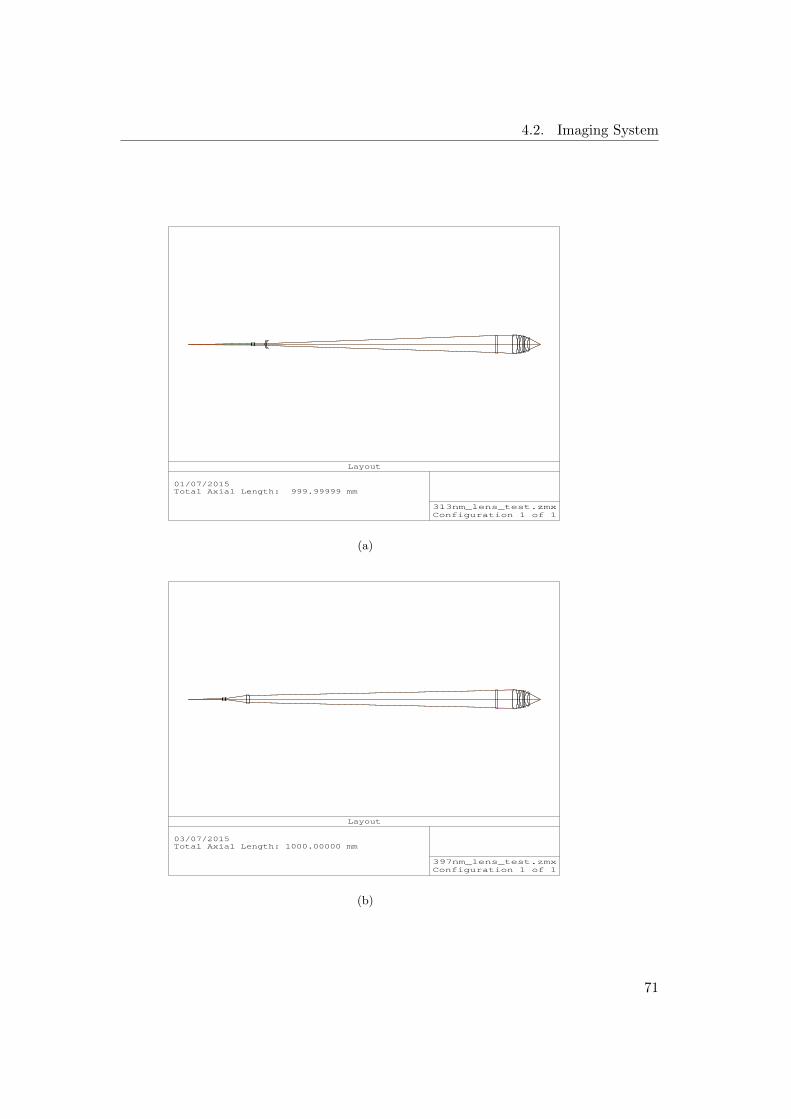
4.2. Imaging System
313nm_lens_test.zmxConfiguration 1 of 1
Layout
01/07/2015Total Axial Length: 999.99999 mm
(a)
397nm_lens_test.zmxConfiguration 1 of 1
Layout
03/07/2015Total Axial Length: 1000.00000 mm
(b)
71

4. Ion Trap and Imaging System
Surface: IMA
20.0
0
0.3130
313nm_lens_test.zmxConfiguration 1 of 1
Full Field Spot Diagram
01/07/2015 Units are µm. Airy Radius: 0.4199 µm
RMS radius : 4.082GEO radius : 5.213Scale bar : 20 Reference : Chief Ray
(c)
Surface: IMA
20.0
0
0.3970
397nm_lens_test.zmxConfiguration 1 of 1
Full Field Spot Diagram
01/07/2015 Units are µm. Airy Radius: 0.5334 µm
RMS radius : 4.088GEO radius : 5.358Scale bar : 20 Reference : Chief Ray
(d)
Figure 4.3: The imaging system design. (a) The layout of the lens design for313 nm light field. (b) The layout of the lens design for 397 nm light field. (c)Simulated spot diagram for 313 nm light field. (d) Simulated spot diagramfor 397 nm light field. Three objects are set 200 µm apart.
72

4.2. Imaging System
does not form an image and enters as an infinity parallel beam in the additionalimage forming lenses (though in our case the objective does not make a perfectinfinity parallel beam, see below). In a finite correction optical system, theobjective lens forms an image by itself. An infinity-corrected objective lenshas the following advantages: 1) A magnification remains the same when thedistance between the objective lens and the additional lens is changed. 2)If a flat plate like the viewport in our case is inserted between the objectivelens and the additional lens, the parfocal point is unchanged and delivers noimage shifts. The two advantages mentioned are significant for configuring anear-diffraction-limited optical system as well as for designing a microscopeoptical system.
Figures 4.3(c) and 4.3(d) show the simulation results of both imaging systemsrespectively. The objects are set to a separation of 200 µm and it forms theimage of 5 µm apart, which is what we should expect because the magnifica-tion is 1/40 (in reverse). All the image spots are within the airy disk, whichis a black circle at the center and is an indication of the diffraction limit. Byreversing the whole system (see Figs. 4.3(a) and 4.3(b)), this is the real situa-tion where the two ions are now the objects with 5 µm apart. The image alsomatches our specifications and we are able to resolve both ions, as shown inFigs. 4.3(c) and 4.3(d).
We then examine how sensitive the focal point is in order to understand thealignment tolerances of the system. We can simulate the spot diagram atdifferent positions crossing the focus. Figures 4.3(a) and 4.3(b) show that itis quite sensitive if we try to adjust the distance between the ion and theobjective. As we can see, with a defocus of 10 µm, the image is already muchlarger than the airy disk. Conversely, if we fix the ion-objective distance, thetolerance of moving the image plane is in the range of millimeters, as shownin Figs. 4.3(c) and 4.3(d).
Construction
Figure 4.4 shows the assembly of the in-vacuum objectives. There are twoidentical imaging systems in our setup, located on two sides of the trap. Onone side the objective can image from zone L1 to the center of the trap; onthe other side, the imaging region is from zone L2 to the center. The totalmovable range of the vacuum bellows is around 3 mm.
Inside the chamber, the objective is screwed in an aluminum mechanicalmount. The whole part is mounted on the flexible vacuum bellows, as shownin the CAD drawing (see Fig. 4.5). As mentioned above, we need the capa-bility to adjust the objective in three dimensions, including the height, thefocal distance, and the axial direction along the trap. Therefore, we attacha three-dimensional translation stage to the bellows. A motorized translation
73

4. Ion Trap and Imaging System
Reverse_313nm_lens.zmxConfiguration 1 of 1
Layout
01/07/2015Total Axial Length: 1000.00000 mm
(a)
Reverse_397nm_lens.zmxConfiguration 1 of 1
Layout
01/07/2015Total Axial Length: 1000.00000 mm
(b)
74

4.2. Imaging System
Surface: IMA
500.
00
0.3130
Reverse_313nm_lens.zmxConfiguration 1 of 1
Full Field Spot Diagram
01/07/2015 Units are µm. Airy Radius: 18.47 µm
RMS radius : 163.381GEO radius : 202.439Scale bar : 500 Reference : Chief Ray
(c)
Surface: IMA
500.
00
0.3970
Reverse_397nm_lens.zmxConfiguration 1 of 1
Full Field Spot Diagram
01/07/2015 Units are µm. Airy Radius: 23.46 µm
RMS radius : 163.662GEO radius : 201.823Scale bar : 500 Reference : Chief Ray
(d)
Figure 4.3: Reversed imaging system. (a) The layout of the lens design for313 nm light field. (b) The layout of the lens design for 397 nm light field. (c)Simulated spot diagram for 313 nm light field. (d) Simulated spot diagramfor 397 nm light field. Three objects are set 5 µm apart, which is a typicalion-ion spacing.
75

4. Ion Trap and Imaging System
Surface: IMA-20 -10 0
<- Defocus in µm ->10 20
0.0000 mm
40.0
0
0.2000 mm
0.5000 mm
313nm_lens_test.zmxConfiguration 1 of 1
Through Focus Spot Diagram
01/07/2015 Units are µm. Airy Radius: 0.4199 µmField : 1 2 3RMS radius : 0.121 0.121 0.123GEO radius : 0.219 0.226 0.241Box width : 40 Reference : Chief Ray
(a)
Surface: IMA-40 -20 0
<- Defocus in µm ->20 40
0.0000 mm10
0.00
0.2000 mm
0.5000 mm
397nm_lens_test.zmxConfiguration 1 of 1
Through Focus Spot Diagram
01/07/2015 Units are µm. Airy Radius: 0.5334 µmField : 1 2 3RMS radius : 0.169 0.168 0.138GEO radius : 0.315 0.366 0.393Box width : 100 Reference : Chief Ray
(b)
76

4.2. Imaging System
Surface: IMA-5000 -2500 0
<- Defocus in µm ->2500 5000
0.0000 mm
200.
00
0.0050 mm
0.0100 mm
Reverse_313nm_lens.zmxConfiguration 1 of 1
Through Focus Spot Diagram
03/07/2015 Units are µm. Airy Radius: 18.47 µmField : 1 2 3RMS radius : 1.274 1.272 1.265GEO radius : 1.664 1.824 1.914Box width : 200 Reference : Chief Ray
(c)
Surface: IMA-5000 -2500 0
<- Defocus in µm ->2500 5000
0.0000 mm
200.
00
0.0050 mm
0.0100 mm
Reverse_397nm_lens.zmxConfiguration 1 of 1
Through Focus Spot Diagram
03/07/2015 Units are µm. Airy Radius: 23.46 µmField : 1 2 3RMS radius : 0.756 0.896 1.357GEO radius : 1.087 1.717 3.098Box width : 200 Reference : Chief Ray
(d)
Figure 4.3: Simulated spot diagrams for the defocus. (a) for 313 nm light field.(b) for 397 nm light field. Reversed the system, and the defocus effect is lesssensitive, shown in (c) for 313 nm and (d) for 397 nm.
77

4. Ion Trap and Imaging System
Ion Position
Figure 4.4: Two identical objectives are set up in the vacuum can and acartoon of where the ions should be. The trap is not mounted in the vacuumchamber and is not shown here.
stage is used for the axial direction for the fine and fast tuning of the position.The other two axes are manually controlled.
Figure 4.6 shows the schematic diagram of a single imaging system. Outsidethe vacuum, both wavelength light fields pass through a vacuum viewportand hit a dichroic beamsplitter4. The diameter of the dichroic beamsplitteris 3 inches and is mounted 45 with respect to the optical table. The lightfield at 313 nm from beryllium ions reflects from the dichroic mirror and the397 nm light field from calcium ions is transmitted. On each arm, there isa pair of lenses as mentioned before, followed by a flip mirror (not shown inthe schematics) to guide the light field into a camera or a photomultipliertube (PMT). Additionally, we insert a dichroic filter5 to filter out the 866 and854 nm scattering light during the qubit readout.
The camera we choose to image the ions is iXon X3 DU897 Electron multi-plying CCD from Andor. It has a pixel number of 512×512 with each pixelsize of 16× 16 µm2. A magnification of 40 onto a pixel size of 16 µm shouldgive us 12.5 pixels between ions for two ions 5 µm apart. Obtained from thesimulation, the diffraction limit is around 1 µm in diameter (double the airyradius), and the image would produce a spot size of 40× 1/16 = 2.5 pixels.
78

4.2. Imaging System
In-vacuum lenses
Flexible bellow Translation
stages
Figure 4.5: Drawing of the assembly of the in-vacuum objectives. Two objec-tives are mounted on the vacuum bellows separately inside the chamber. Athree-dimensional translation stage is attached to the vacuum bellows outsidethe chamber. The ion trap is placed between the objectives, not shown here.(Figure by courtesy of Daniel Kienzler)
First Steps
We unfortunately did not measure the transmission of all the optical elementsfor 313 and 397 nm light fields. It would be good if we know how much loss wehave when performing the qubit readout. Before we tried loading ions, someworks have been done as follows. First, we have to get the position of theobjective right because as described above the distance between the objectiveand the ion is critical. Here we shine and monitor both 313 and 397 nm lighton the trap electrodes simultaneously as shown in Fig. 4.7. By doing so,we could align the position of the imaging system well for both beam paths.In the end, the object is moved back to compensate for the distance of theelectrode front surface and the location of the ion.
4Altechna, www.altechna.com5Semrock, FF01-405/150, alternatively FF01-390/18, which filters out the 423 nm light
too.
79

4. Ion Trap and Imaging System
9Be+
40Ca+
9Be+
PMT & Camera
40Ca+
PMT & Camera
Dichroic beamsplitter
313 nm
1_1-24 mm-313_397nm-3.zmx
Configuration 2 of 3
Layout
19/07/2013
Total Axial Length: 1000.00020 mm
397 nm
Viewport Compensation optics
High NA objective
Dichroic filter
Figure 4.6: Schematics of the whole imaging system on one side of the trap.The second imaging system on the other side is identical to this.
Image 313 nm light Image 397 nm light
Figure 4.7: Illuminating 313 and 397 nm laser fields on the electrode simulta-neously for aligning the imaging system.
Second, in order to observe the neutral fluorescence from the calcium atomsat 423 nm, we can use the same imaging system. According to the Zemax sim-ulation, the diffraction limited resolution can also be achieved for the 423 nmlight field by translating the objective by 0.32 mm backwards. Figure 4.8shows the atom cloud fluorescing at 423 nm on the calcium camera.
Ion Imaging
After the laser systems (see Chapter 5) and the control system (see Section4.3) were prepared and ready to use, we successfully loaded a two-species ion
80

4.2. Imaging System
Figure 4.8: Neutral calcium fluorescence at 423 nm is observed by translatingthe objective by 0.32 mm.
chain in the segmented ion trap. As shown in Fig. 4.9, the ion chain containstwo calcium ions and one beryllium ion. They were imaged simultaneouslyon separate cameras. On the calcium camera, the picture shows two calciumions, and the dark region in the middle is where the single beryllium ion islocated. The details of loading process can be found in Chapter 6.
9Be+ ion
40Ca+ ions
Mixed-species ion chain
9Be+ 40Ca+ 40Ca+
Figure 4.9: Pictures of two 40Ca+ ions and one 9Be+ ion trapped simultane-ously in the same potential well. The calcium camera shows the image of twotrapped 40Ca+ ions, and a dark 9Be+ ion in the middle can not be observed.The beryllium camera shows a single trapped 9Be+ ion surrounded by the twodark 40Ca+ ions.
Figure 4.10 shows the image of an ion string, where we can see each ion hasa fan-shaped tail. We notice that the image quality is very sensitive to atilt to the objective. This effect is then examined in the simulation. Weconsider a case in which the objective has a tilt of 0.2. Figure 4.10 shows
81

4. Ion Trap and Imaging System
the simulated spot diagram for the calcium arm, for which I set three objectswith 5 µm apart. It can be seen that the resulting image also has a tail andis not circularly symmetric anymore. The direction of the tail depends onwhere the objective is tilted. Consequently, we need to take special care ofthe objective during the vacuum bake-out and mounting of the componentsin order to avoid any tilt. This slightly image distortion does not cause severeproblems in our experiments.
(a)
Surface: IMA
1000
.00
0.3970
Reverse_397nm_lens_obj_tilted.zmxConfiguration 1 of 1
Full Field Spot Diagram
02/07/2015 Units are µm. Airy Radius: 22.38 µm
RMS radius : 177.500GEO radius : 294.460Scale bar : 1000 Reference : Chief Ray
(b)
Figure 4.10: (a) Image of three 40Ca+ ions. There is a dark ion in the trap,and each ion has a fan-shaped tail. (b) Simulation of the spot diagram in casethe objective is tilted. The parameter used here is the tilted angle of 0.2.
82

4.3. Experimental Control
Photon Detection
We use PMTs from Hamamatsu6, and the model we have is H10682-210. Ithas an active area of 8 mm in diameter. The count sensitivity at 397 nm and313 nm is 6×10⁵ and 4×10⁵ s−1pW−1, respectively. These values have takenthe quantum efficiency and collection efficiency into account. As a result, thetotal detection efficiency of the PMT per photon is 30 % for 397 nm and isaround 26.5 % for 313 nm .
The total detection efficiency ζ used in Chapter 2.4 can be calculated with
ζ = effective solid angle 4.4%×PMT quantum efficiency 26.5%×assuming 15% loss in optics and windows (1− 15%)
' 0.01
We can now estimate the mean photon number which is collected during thequbit readout if the ion is in the bright state. In the case of beryllium ions,from Eq. (2.6) we have the photon scattering rate Γ = γ/6 with s0 = 0.5.So the mean photon number we detect can be estimated by N = ζτDΓ ' 40photons with the duration of the detection pulse τD = 200 µs. For calciumions, Γ = γρP1/2
, where ρP1/2is the P1/2 state populations, and we can see from
the simulation results in Chapter 3.3 the maximum ρP1/2under our working
conditions is around 0.1. Therefore, the mean photon number we can collectduring the calcium qubit readout is N ' 30. Both estimations agree withwhat we observe in the experiment. We use this detection time of 200 µs inorder to better distinguish the ion being dark or bright. A more careful studyabout the qubit readout fidelity of 9Be+ ions is given in Chapter 6.2.
4.3 Experimental Control
The experiments we are doing in our group require a high level of control. Ingeneral, well-controlled laser frequency and phase, the duration of the laserpulse, voltage waveforms, and digital acquisition of data are necessary. Toaccommodate all of the required capabilities, we employ a field programmablegate array (FPGA) based experiment controller for use in the experimentswith trapped ions.
The core of the computer control system uses the ML507 evaluation plate-form7, which contains Virtex-5 FPGAs and a PowerPC 440 processor. TheFPGA-based control system can produce a timing-critical pulse sequence. Itis convenient to program and powerful, where the users write a pulse sequence
6Hamamatsu, www.hamamatsu.com7Xilinx, www.xilinx.com
83

4. Ion Trap and Imaging System
in C/C++. The ML507 board is controlled via ethernet through a graphicaluser interface (GUI) on a standard PC. The GUI software we use is called“Ionizer”, which allows users to set the parameters and run the experiments.It was originally developed by NIST Ion Storage Group and further improvedby Ben Keitch, Vlad Negnevitsky and Matteo Marinelli. The codes of theGUI software were written in QT and C++.
The laser pulse duration is controlled by a TTL pulse (transistor-transistorlogic) output from FPGA. The TTL pulse controls RF-switches, which switchon and off RF signals passing to the AOM in the laser setup. The laserfrequency, phase and amplitude are modulated with the RF signal which issent into the AOM from direct digital synthesizer (DDS) boards8.
As a temporary solution used in our phase of experiments, the DDS boardsare preloaded with frequency, phase and amplitude settings. They allow aTTL signal for a DDS channel to switch to another setting, where the phaseis referenced to the first setting. These RF signals are sent to the AOMs formodulating the frequency, phase and amplitude of the laser in an experimentalsequence. The limitations are that we can not update parameters (excepttime) during a sequence, there are only two profiles per DDS channel, and ituses an USB connection, which is slow. In this temporary setup, the phaseswitched between two DDS profiles is not coherent, and the starting phase ofthe first pulse of a DDS channel is random and the following pulses have aabsolute phase reference to the first one if we keep running the same profile.
The whole computer control system is now upgraded, including the firmwareof the DDS board and the FPGA board. Now the new system is much moreflexible and powerful. The phase, frequency and amplitude sent to one AOMcan be changed only with one DDS channel while running an experimentalsequence, which we could not do in the past. This will facilitate more complexexperiments in the future.
8Enterpoint, Milldown DDS board, www.enterpoint.co.uk
84

Chapter 5
Beryllium Laser Systems
Lasers are used for ionization, cooling and quantum state manipulation of ions.A stable and controllable laser system is an indispensable part for all of theexperiments with trapped ions or atoms. In our group, since we work with twospecies of ions, more wavelengths and setups are involved in the laser systems.During my PhD, I developed laser systems and setup all the beam lines forcontrol of beryllium ions. In this chapter, I will first describe an overview ofour laser setup configuration and then focus on the work that I have done.Some of the sections are covered in our publication [Lo 14]. The calciumlaser systems used in our group include contributions from many people. Thedetails can be found in [Kienzler 15b, Sepiol 12, Lindenfelser 11].
One of the major challenges of working with beryllium is that the lowest-energy transitions for excitation from the ground state of both the ion andthe atom require wavelengths in the ultraviolet (UV) region of the spectrum,at 313 and 235 nm respectively (Fig. 5.1). As a result, most experimentsperformed until now have required frequency doubled dye lasers for control ofthe ion. Photoionization of neutral beryllium has been previously performedusing a frequency-quadrupled pulsed Titanium-Sapphire laser [Blakestad 10].These laser systems are expensive and complex, motivating the use of alter-native approaches. Here I will present a new setup for generating continuous-wave (CW) 235 nm light for photoionization of beryllium atoms based on twostages of frequency doubling of light from a diode laser. In addition, for con-trolling beryllium ions, we follow the approach demonstrated by Wilson et al.[Wilson 11] to generate three desired UV wavelengths at 313 nm starting fromfour infrared (IR) fiber-laser sources. The latter complements recent develop-ments using telecom lasers at 1565 nm [Vasilyev 11] or diode lasers at 626 nm[Ball 13], with the advantage that the powers we achieve are far higher. I willpresent how we stabilize the frequency of the 313 nm light. Once the lightat the fundamental laser frequency has been generated, it is delivered to theions via acousto-optic modulators (AOMs) for frequency fine-tuning and laser
85

5. Beryllium Laser Systems
235 nm
235 nm
Con)nuum
197.2 GHz
9Be+ 9Be
Repumping (313.197 nm)
Tuning range
Δ = -‐70 GHz
Cooling & Detec)on (313.133 nm)
Δ = -‐380 GHz
Raman (313.273 nm)
307 nm
2p 1P1
2s 1S0 2S1/2
2P1/2
2P3/2
Figure 5.1: Relevant level schemes in beryllium. Left: two-photon ionizationprocess by resonant excitation from 1S0 to 1P1 in neutral 9Be. Right: 9Be+
energy levels addressed during trapping and manipulation.
pulse control. I will describe three AOM beam line setups for control of beryl-lium ions, including cooling/detection beams, repumping beams, and Ramanbeams.
5.1 Overview
Our vacuum chamber has 6 optical ports which can be accessed by the laserbeams. A schematic of the laser arrangements is shown in Fig. 5.2. Wecombine calcium and beryllium laser beams on the dichroic beamsplitter whichis the same as the one in the imaging system. This dichroic beamsplitter isdesigned for 397 nm and 313 nm light fields. It also works for all the calciumlaser wavelengths with some power loss. However, the coating of this dichroicbeamsplitter does not reflect 235 nm light. For Port 1, we use a dichroicbeamsplitter1 for which the reflection band is from 230 to 325 nm and thetransmission band is from 380 nm to near-infrared. The calcium laser beamsentering from this port are linearly polarized. For the horizontal polarizationcomponent, the ion experiences π polarized light. If the laser is verticallypolarized, the ion will experience a superposition of σ+ and σ−.
For the cooling, detection, and repumping beams applied to beryllium ions,we require pure σ+ polarized light. This requirement can only be fulfilled by
1Semrock FF347-Di01, www.semrock.com
86

5.2. Laser Source at 235 nm
Ion pump &
Atomic oven
connections
DC & Shim
electrode
feedthrough
Port 6
Imaging system
Port 5
Imaging system
Trap axis
B fields
B fields
Ca+: 729 nm
Be+: BDD, BD,
RD1, RD2
Ca+: 397, 854, 866,
375, 423 nm
Be+: Retro-reflective
Raman, 235 nm
Be+: Raman 90
Ca+: 397 nm
Be+: Raman Co, 90
Port 1
Port 3
Port 4
Port 2
Figure 5.2: Laser beam configurations near the vacuum chamber.
sending the laser beam parallel to the magnetic field. Here we use Port 2, asshown in Fig. 5.2. The 729 nm laser beam for calcium qubit manipulationsuses the same port, but the polarization of this beam is not critical for ourparticular choice of beam direction relative to the magnetic field [Roos 00b].
The Raman beams for controlling the beryllium qubit are illuminated fromPort 3 and 4. To drive a single-qubit rotation, two co-propagating Ramanbeams are sent from Port 3. Implementation of sideband cooling or a twoqubit gate with beryllium ions needs two Raman beams perpendicular to eachother or counter-propagated, where the difference of two k vectors is non-zero.Therefore, one beam is sent from Port 3 and the other one is sent from Port4.
Apart from the regular setup described above, the additional 397 nm laserbeam in Port 4 is used for electromagnetically-induced-transparency (EIT)cooling [Roos 00a], and we retro-reflect the two co-propating Raman beamsfrom Port 1 to demonstrate parallel single-qubit quantum operations usingtransported ions [de Clercq 15].
5.2 Laser Source at 235 nm
Ionization of neutral beryllium atoms requires an energy of 9.3 eV, correspond-ing to a wavelength of 133 nm. Since this wavelength lies in the vacuum UV,
87
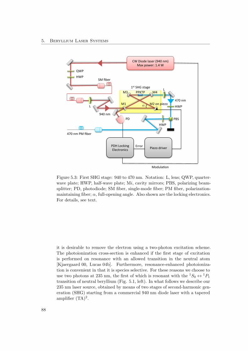
5. Beryllium Laser Systems
Error PDH Locking Electronics Piezo driver
CW Diode laser (940 nm) Max power: 1.4 W
QWP
HWP
HWP
HWP
PBS
SM fiber
470 nm PM fiber
1st SHG stage
M1 M2 on piezo
M3 M4
PD
ModulaOon
L
L PPKTP
470 nm
940 nm
α
Figure 5.3: First SHG stage: 940 to 470 nm. Notation: L, lens; QWP, quarter-wave plate; HWP, half-wave plate; Mi, cavity mirrors; PBS, polarizing beam-splitter; PD, photodiode; SM fiber, single-mode fiber; PM fiber, polarization-maintaining fiber; α, full-opening angle. Also shown are the locking electronics.For details, see text.
it is desirable to remove the electron using a two-photon excitation scheme.The photoionization cross-section is enhanced if the first stage of excitationis performed on resonance with an allowed transition in the neutral atom[Kjaergaard 00, Lucas 04b]. Furthermore, resonance-enhanced photoioniza-tion is convenient in that it is species selective. For these reasons we choose touse two photons at 235 nm, the first of which is resonant with the 1S0 ↔ 1P1
transition of neutral beryllium (Fig. 5.1, left). In what follows we describe our235 nm laser source, obtained by means of two stages of second-harmonic gen-eration (SHG) starting from a commercial 940 nm diode laser with a taperedamplifier (TA)2.
88

5.2. Laser Source at 235 nm
5.2.1 First SHG Stage: 940 to 470 nm
The first stage of frequency doubling converts 940 into 470 nm light. Aschematic of the experimental setup is shown in Fig. 5.3. The Toptica TA unitcan deliver up to 1.4 W at 940 nm. We first pass this light through a single-mode (SM) fiber to clean up the spatial mode, resulting in up to 700 mWwhich can be sent to a bowtie cavity for power build-up. The frequency con-version is performed using a periodically-poled potassium titanyl phosphate(PPKTP) crystal, chosen due to its high non-linearity and transparency atboth 940 and 470 nm. The PPKTP crystal3 has a 5.95 µm poling period andis temperature stabilized close to 21C for quasi-phase matching (QPM).
The cavity was designed by Joseba Alonso. The cavity’s geometry is opti-mized to achieve high conversion efficiency while minimizing the dependenceof the second-harmonic output power on the short arm optical length (M3-M4) [Wilson 11]. QPM is intrinsically free of walk-off (the Poynting andpropagation vectors of the second-harmonic field are parallel), so a value forthe Boyd-Kleinmann focusing parameter of ξ = 2.84 should yield the maxi-mum conversion efficiency [Boyd 68]. This parameter is defined as ξ ≡ lc/b,with lc the crystal length and b = 2πnωw
2/λ the confocal parameter of thelaser beam. Here nω is the refractive index of the crystal sampled by theinput light (of wavelength λ) and w the waist size of the beam in the crys-tal. Based on previous observations of thermal lensing effects in a similarsystem operated at 922 nm by Le-Targat et al. [Targat 05], we designed thecavity for a larger waist of w = 50 µm (ξ = 0.98) to reduce the intensityof the generated blue light inside the crystal. The curved mirrors introduceastigmatism to the beam, which we minimize by using a small opening an-gle α ≈ 11 (see Fig. 5.3), limited by geometric constraints imposed by themirror-mounts. The transmission of the input coupling mirror M1 was chosento be T1 = 14.5 % in order to account for the expected cavity losses, and thusachieve an optimal impedance matching to the cavity for a predicted inputpower of P940 = 600 mW. More details of the cavity design are given in Table5.1.
The length of the cavity is locked to the pump laser using the Pound-Drever-Hall (PDH) technique [Drever 83]. The 940 nm diode is phase-modulated at15.6 MHz via a bias-tee input to the diode current. The light reflected fromthe cavity is collected by a fast photodiode and the signal is demodulatedand filtered. The error signal thereby produced is used to feed back on thepiezoelectric stack to which M2 is glued.
The results for this first stage of frequency doubling are shown in Fig. 5.4,including both the second-harmonic output power P470 and the ratio η470 =
2Toptica, www.toptica.com3Raicol Crystal Ltd., raicol.com
89

5. Beryllium Laser Systems
1 0 0 2 0 0 3 0 0 4 0 0 5 0 0 6 0 0 7 0 00
1 02 03 04 05 06 07 08 0
U n s t a b l e l o c kd u e t o t h e r m a l l e n s i n g
470 (%
)
P 9 4 0 ( m W )
S t a b l e l o c k
0
1 0 0
2 0 0
3 0 0
4 0 0
5 0 0
6 0 0
P 470 (m
W)
Figure 5.4: Measured net power at 470 nm (triangles, referred to the right axis)and the power ratio of the 940→ 470 nm doubling cavity (circles, referred tothe left axis) as a function of the pump power. The solid line corresponds tothe theoretical prediction of η470 based on Eq. (C.5) in the Appendix C. Tothe right of the vertical line the cavity becomes unstable (see text).
P470/P940 as a function of the input power P940. The solid line results from thetheoretical calculation using the theory given by Le-Targat et al. [Targat 05],which generalized the seminal work of Boyd and Kleinmann [Boyd 68] to asituation including an optical cavity [Freegarde 01]. Our calculations use thecavity parameters and the crystal properties provided by the manufacturer.These are displayed in Tables 5.1 and C.1. The theory is summarized in theappendix.
It is worth noting that, as was observed previously in a similar system operatedat 466 nm [Targat 05], the output power is limited by thermal lensing inducedby absorption of the 470 nm light in the crystal. Our cavity becomes unstablefor P470 > 400 mW. For stable operation, we set P940 ≈ 500 mW and obtainP470 ≈ 350 mW (η470 ≈ 70 %).
5.2.2 Second SHG Stage: 470 to 235 nm
The 470 nm light generated in the first SHG stage is sent through a 30 m longpolarization-maintaining (PM) fiber (OZ Optics) to a neighboring laboratory.The output mode of the fiber is matched to the spatial mode of the secondbowtie cavity with a two-lens telescope, and the polarization is cleaned usinga polarizing beam-splitter (PBS) cube (see Fig. 5.5). Input-coupling lossesand absorption in the fiber result in a maximum value of ≈ 140 mW of lightincident on the 470→235 nm cavity.
90

5.2. Laser Source at 235 nm
Table 5.1: Details of the cavities for SHG of 470 and 235 nm light. All mirrorcoatings were provided by Layertec GmbH. wh,v are the horizontal and verticalbeam waists.
940→470 nm 470→235 nm
Crystal Material PPKTP BBOPhase-matching QPM (type I) CPM (type I)
Dimensions 1× 2× 30 mm3 4× 4× 10 mm3
Phase-matching angles θ/φ 90/0 58.15/0
Surfaces AR coated @ 940 nm Brewster-cut (59.25)Temperature stabilization 0.1C (@ 21C) Not stabilized
Mirrors Radius of curvature M3 & M4 100 mm 38 mmReflectivity M1 85.5 % 99.0 %Coating M2-M4 Sputter Ion-beam sputter
Cavity Long arm length 399 mm 320 mmCrystal-mirror distance 50 mm 18 mmFull opening angle (α) 11.0 33.8
Mean waist short/long arm 50/212 µm 18/145 µmElipticity short/long arm (wh/wv) 0.99/0.96 1.53/1.00
Full spectral range (FSR) 560 MHz 805 MHzLinewidth 43 MHz 2.7 MHz
Finesse (F) 13 300
Piezo driver PDH Locking Electronics
470 nm PM fiber
2nd SHG stage
PD
PBS
L L
Error
M1 M2 on piezo
M3 M4 L
Dichroic mirror
470 nm
235 nm
BBO
α
Figure 5.5: Second SHG stage: 470 to 235 nm. Labels are as in Fig. 5.3. Fordetails, see text.
91

5. Beryllium Laser Systems
2 0 4 0 6 0 8 0 1 0 0 1 2 0 1 4 00
4
8
1 2
1 6
2 0
2 4
235 (%
)
P 4 7 0 ( m W )
051 01 52 02 53 03 5
P 235 (m
W)
Figure 5.6: Measured net power at 235 nm (triangles, referred to the right axis)and the power ratio of the 470→235 nm doubling cavity (circles, referred tothe left axis) versus the pump power at 470 nm. The solid line correspondsto the theoretical prediction of η235 based on Eq. (C.5) in the Appendix C.
For this SHG stage we use a BBO crystal (Castech Inc.) Brewster-cut for470 nm which achieves critical type-I phase matching (CPM) at an angle of58.15. This cavity was also designed to optimize the conversion efficiencyof the frequency doubling while being insensitive to changes in the positionsof the focusing mirrors M3 & M4 [Wilson 11]. By contrast with the firstfrequency-doubling stage, the use of angle phase-matching intrinsically resultsin walk-off which limits the length of the conversion region of the crystal. Theoptimized cavity parameters are given in Table 5.1. The length of the cavityis also stabilized using the PDH method in order to keep it on resonancewith the pump laser. Since the modulation frequency applied to the diodelaser (15.6 MHz) is comparable to the linewidth of the 940→470 nm cavity,the 470 nm light also exhibits modulation sidebands at 15.6 MHz and can bedirectly used for the PDH locking scheme.
Figure 5.6 shows the UV output power P235 along with the power ratio η235 =P235/P470 as a function of the input power P470. Note that we define P235 andη235 in terms of the net second-harmonic power at the output of the cavity.With P470 ≈ 140 mW, we obtain P235 ≈ 28 mW (η235 ≈ 20 %). Consideringthe 22 % reflection at the output surface of the Brewster-cut BBO crystal,the total UV light generated is ≈ 36 mW. The theoretical curve is calculatedusing the values given in Table C.1, yielding Γeff ≈ 1.6× 10⁻⁴ W−1. The levelof agreement between the measured values of η235 and those predicted by thetheory is reasonable given the assumptions made in the theory, which include
92

5.3. Laser Source at 313 nm
perfect phase-matching of a circular beam and no absorption in the crystal(see Table C.1).
The counter-propagating fundamental mode of a bowtie cavity can be excitedby any back-reflecting element in the cavity, which can lead to considerableback-circulating power if the finesse F of the cavity is high [Hemmerich 90].In the 470→235 nm cavity, we observe that light is emitted along a directionwhich is consistent with this effect. This leads to a reduction in η235 and anunstable output power. The back-circulation could likely be eliminated byreducing the reflectivity of M1 if required [Hemmerich 90]. Since photoioniza-tion does not require high stability or high power, we have currently chosennot to pursue this.
The power we achieve is comparable to the average power of the pulsed laserused in [Blakestad 10], and considerably higher than values which have beenpreviously used to perform photoionization of other atomic species [Lucas 04b,Kjaergaard 00]. The 1S0 ↔1P1 transition of neutral beryllium atoms has asaturation intensity of 8.9 mW/mm2, corresponding to 70 µW for a beamwaist of 50 µm.
5.3 Laser Source at 313 nm
Quantum control experiments using beryllium ions require near resonant lightfor Doppler cooling and optical pumping and, in our case, a far-detuned Ra-man laser for coherent manipulations [Wineland 98]. As shown in Fig. 5.1(right), the wavelengths of the 2S1/2 ↔ 2P3/2 and 2S1/2 ↔ 2P1/2 transitionsare at 313.133 nm and 313.197 nm, respectively. We have chosen to operateour Raman laser system at a wavelength between 313.221 and 313.322 nm,detuned to the red of the 2P1/2 manifold by between −380 and −70 GHz.Small detunings allow for lower power for a given Raman transition rate, butlead to more spontaneous scattering of photons which will induce errors in thequantum state manipulation. Therefore, for high-fidelity control of a quantumsystem, a large detuning from the excited state is preferable [Ozeri 07]. Thelaser systems to generate all three wavelengths are shown schematically in Fig.5.7.
5.3.1 SFG Stage: Infrared to 626 nm
To produce the three UV wavelengths we require, we start from four fiberlasers4 at 1550.65 nm, 1050.56 nm, 1551.44 nm and 1050.98 nm which can bethermally tuned over a range of 80 GHz and fine-tuned over ±150 MHz bymeans of an internal piezoelectric element. The laser outputs (PM fibers)are terminated with an integrated beam-collimation system, producing beams
4NP Photonics, www.npphotonics.com
93

5. Beryllium Laser Systems
626.546 nm
HWP DBS
CW Fiber laser (1550.65 nm) Max power: 5 W
CW Fiber laser (1551.44 nm) Max power: 10 W
CW Fiber laser (1050.56 nm) Max power: 10 W
CW Fiber laser (1050.98 nm) Max power: 10 W
HWP HWP
DBS
PBS
HWP HWP
DBS
PBS
SHG stage M1 M2 on piezo
M4 M3 L
SFG stage
626.394 nm
626.266 nm
313.273 nm
313.197 nm
313.133 nm
Raman
Repumping
Cooling & DetecOon
EOM
EOM
EOM
HWP PBS
Iodine spectroscopy
HWP PBS
Iodine spectroscopy
HWP
BBO
PPLN + oven
PPLN + oven
PPLN + oven
PC fiber
SM fiber
SM fiber
Figure 5.7: Setup for generating three wavelengths at 313 nm for Dopplercooling, optical pumping and coherent manipulations of beryllium ions. No-tation: DBS, dichroic beam-splitter; EOM, electro-optic modulator; PC fiber,photonic-crystal fiber; the rest are as in Fig. 5.3. The locking electronicsand focusing lenses are not shown. The wavelengths indicated for the Ramansetup are approximately in the middle of the range of operation. For details,see text.
of diameters between 3 and 4 mm. The sum-frequency generation (SFG) isperformed using magnesium-oxide-doped periodically-poled lithium niobate(MgO:PPLN) crystals5. Each crystal contains three different poling periodsof around 11.5 µm on strips 1 mm wide which run down the length of the4 cm long crystal. The PPLN crystals are maintained at a constant operatingtemperature in order to achieve the phase-matching condition for maximizingthe conversion efficiency. In our case, we obtain maximal 626 nm outputpower for temperatures close to 180C, stabilized to within ±0.01C. In orderto access the highest non-linear coefficient of the crystal, the polarization axisof the light is parallel to the thickness of the crystal.
The 1050.56 nm light is shared between the cooling and repumping setups(Fig. 5.7). The power ratio can be tuned by rotating the half-wave plate infront of the PBS. The same mechanism applies for the 1551.44 nm laser, whichis split between the repumping and Raman setups. In all three setups, two ofthe fiber-laser outputs (pump beams) are overlapped using a dichroic elementafter passing through independent beam-shaping telescopes (not shown in thefigure) that focus the beam to an optimal waist inside the crystal. The beamwaist that maximizes the conversion efficiency was experimentally found to
5Covesion Ltd., www.covesion.com
94

5.3. Laser Source at 313 nm
0 1 0 2 0 3 0 4 0 5 0 6 0 7 0 8 02 . 4
2 . 6
2 . 8
3 . 0
3 . 2
3 . 4
3 . 6
SFG (%
W -1
cm-1 )
P 1 0 5 0 . 9 8 x P 1 5 5 1 . 4 4 ( W 2 )
012345678
P 626.5
4 (W)
Figure 5.8: Net power of 626 nm light measured at the output as a function ofthe product of pump powers (triangles, referred to the right axis). Also shown(circles, referred to the left axis) is the sum-frequency-generation efficiency perunit length of the crystal.
be 58± 5 µm at the center of the crystal. This is larger than the 40 µmpredicted from the Boyd-Kleinmann theory. A possible explanation for thisdifference could be phase mismatch or imperfect spatial-mode overlap arisingfrom absorption-induced heating in the crystal [Batchko 98].
All SFG setups exhibit similar performance. For the Raman light (SFG of the1050.98 nm and 1551.44 nm) the output power for different products of thepump powers is plotted in Fig. 5.8. We have generated up to 7.2 W of redlight at 626.54 nm using pump powers of 8.5 W at 1050.98 nm and 8.3 W at1551.44 nm. Also shown is the conversion efficiency per unit length
ΓSFG =P626
P1051P1551lc, (5.1)
which characterizes the performance of the non-linear crystal. We find a maxi-mum value of ΓSFG ≈ 3.5 % W−1cm−1, which is reduced to≈ 2.5 % W−1cm−1
at the highest output power, possibly due to absorption-induced heating inthe crystal. To test whether these effects are more prominent in the IR or thevisible light, we measured ΓSFG for different combinations of pump powerswith a constant product P1050.98 × P1551.44, which would be expected to pro-duce the same amount of red light. The results (see Fig. 5.10) show that theconversion efficiency is lowest when P1551.44 > P1050.98. The Pearson correla-tion coefficients Rλ between ΓSFG and the pump powers are R1050.98 ≈ −0.5and R1551.44 ≈ −0.9, indicating that the absorption of the 1551.44 nm lightcontributes most to thermal effects.
95

5. Beryllium Laser Systems
Temperature (oC)
179.5 180 180.5 181 181.5 182 182.5
Norm
aliz
ed 6
26 n
m p
ow
er
0
0.2
0.4
0.6
0.8
1
(a)
Temperature (oC)
180 180.5 181 181.5 182 182.5
Norm
aliz
ed 6
26 n
m p
ow
er
0
0.2
0.4
0.6
0.8
1
(b)
Figure 5.9: Temperature dependence of the Raman sum frequency generationsetup. The 626 nm power is normalized to 1. The PPLN nonlinear crystal ismounted in the oven and the temperature is controlled with a PID-regulatedthermoelectric in a step of 0.01 (a) High pump powers. (b) Low pump powers.
We also measure the temperature dependence of the SFG in the Raman setupwith two different pump power settings. Figure 5.9 shows the experimentalresults, where the 626 nm power is normalized to 1 for both cases. We can seethat with high pump powers the temperature of getting maximum conversionefficiency goes down. This can be explained by the fact that higher pumppower heats up the nonlinear crystal more strongly. So we should set the tem-perature lower in order to fulfill the phase-matching condition. The observedasymmetry in the case of high pump powers is due to spread of the wavevec-tors in the focused beam, since the phase-matching conditions are fulfilled atdifferent temperatures for different wavevector components of the pump beam[Schuck 10, Gibson 98].
At an output power of ≈ 7 W the drift was observed to be below 0.2 % perhour over 10 hours of operation. After running this system for more than ayear at a variety of input and output powers, we have seen little change in theconversion efficiency, and no realignment of the optical components has beenrequired.
Since the detection and repumping beams must provide light resonant withthe 2S1/2 ↔ 2P3/2 and 2S1/2 ↔ 2P1/2 transitions, the absolute frequencies ofthese lasers must be actively stabilized. The transition linewidths are γ/2π ≈19.4 MHz, so we aim for frequency stability on the level of a megahertz. Tothat end, a small portion of the 626 nm light is picked off and sent through anoptical fiber to a Doppler-free saturated-absorption-spectroscopy setup withan iodine cell [Demtroeder 82, King 99]. This will be discussed later in thischapter. However, in the Raman setup the stability of the absolute frequency
96

5.3. Laser Source at 313 nm
1 2 3 4 5 6 7 81
2
3
4
5
6
7
8
S F G
P 1551
.44 (W
)
P 1 0 5 0 . 9 8 ( W )
2 . 6 4 4
2 . 8 5 8
3 . 0 7 2
3 . 2 8 6
3 . 5 0 0
( % W - 1 c m - 1 )
Figure 5.10: Conversion efficiency per unit length of the crystal measuredfor different pump powers. The dashed lines correspond to combinations ofP1551.44 and P1050.98 with a constant product. The data points were takenalong these curves.
is not as critical due to the large detuning from resonance, and the naturalstability of the fiber lasers (which we have measured to drift by less than60 MHz over a day) is sufficient for our purposes.
5.3.2 SHG stage: 626 to 313 nm
The beams from the SFG setups are coupled into high-power SM fibers andsent to frequency doubling cavities for conversion to 313 nm. The couplingefficiency is ≈ 90 % in the repumping and cooling setups excluding the loss inthe fiber collimators (5 m long SM fibers6). This is because the high qualityGaussian modes of the pump beams produced by the fiber lasers is trans-ferred to the 626 nm light. Measurement of the spatial mode of the output626 nm light is shown in Fig. 5.11, measured with a beam profiler. The powertransmitted through the fibers saturates at ≈ 2 W due to stimulated Brillouinscattering [Agrawal 07]. It is interesting that we observe the frequency of thereflected light from the fiber is shifted by 27 GHz, which is measured with awavelength meter. In order to avoid this problem in the Raman setup, wherewe require higher powers, we use a photonic-crystal fiber7. The limitation isin this case the coupling efficiency into the fiber, which is ≈ 60 %.
6OZ Optics, www.ozoptics.com7NKT Photonics, www.nktphotonics.com
97

5. Beryllium Laser Systems
Figure 5.11: The beam profile of the 626 nm light measured with a beamprofiler.
SHG from 626 to 313 nm is performed in all three cases using a BBO crystalBrewster-cut for 626 nm with a phase-matching angle of 38.35. The crystalsare placed in bowtie cavities (FSR ≈ 845 MHz and F ≈ 275) for pump-powerenhancement. The beam waists in the BBO crystals are 36.7 (23.6) µm forthe horizontal (vertical) direction. The design and properties of the doublingcavities are very similar to those reported by [Wilson 11] except that we usea Pound-Drever-Hall rather than Hansch-Couillaud scheme to stabilize thecavity length. In order to generate the required modulation for the PDH sta-bilization, we pass the 626 nm beams through electro-optic phase modulators(Qubig) placed directly after the PPLN crystals and driven at frequenciesclosed to 125 MHz. All of the SHG conversion setups are similar, so below wegive explicit details for the Raman setup, for which we work with the highestpowers.
Figure 5.12 shows the 313 nm output power P313 and the power ratio η313 =P313/P626 as a function of the power P626 coupled into the Raman doubling cav-ity. As before, P313 and η313 are defined in terms of the net second-harmonicpower delivered by the system. The maximum output power obtained is≈ 1.95 W, with P626 ≈ 3.8 W (η313 ≈ 52 %). Including the 20 % reflection atthe output facet of the Brewster-cut BBO crystal, overall ≈ 2.4 W at 313 nmare produced. The parameters for the theoretical calculation of Eq. (C.5) aregiven in Table C.1.
In order to characterize the long-term performance of the UV light production,we have monitored the stability of the 313 nm power. For these tests, outputpowers up to P313 ≈ 1 W (P626 ≈ 2.2 W) were used. Observed drifts werebelow 0.5 % per hour during 8 hours of continuous operation.
98

5.4. Iodine Spectroscopy
0 5 0 0 1 0 0 0 1 5 0 0 2 0 0 0 2 5 0 0 3 0 0 0 3 5 0 0 4 0 0 01 0
2 0
3 0
4 0
5 0
6 0
313 (%
)
P 6 2 6 ( m W )
0
5 0 0
1 0 0 0
1 5 0 0
2 0 0 0
P 313 (m
W)
Figure 5.12: Measured net power at 313 nm (triangles, referred to the rightaxis) and the power ratio of the 626→313 nm Raman doubling cavity (circles,referred to the left axis) versus the input power at 626 nm. The solid linecorresponds to the theoretical prediction of η313 based on Eq. (C.5) in theAppendix C.
5.4 Iodine Spectroscopy
Since the detection and repumping beams provide light resonant with the2S1/2 ↔ 2P3/2 and 2S1/2 ↔ 2P1/2 transitions of the beryllium ion, the ab-solute frequencies of these lasers must be actively stabilized. The transitionlinewidths are γ/2π ≈ 19.4 MHz, so we aim for frequency stability on thelevel of a megahertz. To that end, precision spectroscopy can be used toprovide a very stable frequency reference for a laser. Here we do not sta-bilize the frequency of 313 nm light directly. Instead a small portion ofthe 626 nm light is picked off and sent through a single-mode fiber to aDoppler-free saturated absorption spectroscopy setup with an iodine vaporcell [Demtroeder 82, King 99].
The optical setup is shown in Fig. 5.13. The 626 nm light out of fiber firstpasses through a half-wave plate and a PBS, where the half-wave plate is usedto clean up the polarization of the light and make sure the transmitted poweris maximum. Then the beam is focused into an AOM, followed by anotherlens collimating the beam. It is passed through a quarter-wave plate andreflected from a mirror. The polarization of the light in the second pass haschanged from horizontally polarized to vertically polarized by passing throughquarter-wave plate twice. It is then picked off from the reflection port of thePBS. This double-pass configuration is different from the one we use for theUV light (see next Section) since the AOM for this wavelength can take any
99

5. Beryllium Laser Systems
SMF
HWP PBS L-1 AOM-1 L-2 QWP
M
PBS HWP
BK7
Window
AOM-2
Iodine Cell
Auto-balanced
photodiode
SMF
Wavelength
meter
Figure 5.13: The optical setup for the iodine saturated absorption spec-troscopy. For details, see text.
polarization with no change in the diffraction efficiency. This double-passAOM produces a frequency offset of ∆f = −2 × 388.5 MHz and allows us tochange the frequency offset between the laser light and the iodine lock. Thebeam reflected from the PBS passes through a 5-mm thick glass window (ap-proximately 5 % reflectance per surface). Two weak reflected beams are theprobe and reference beams for the saturated absorption spectroscopy. Thetransmitted beam, which is called pump beam, has more power and passesthrough another single-pass AOM. The radio frequency applied to this AOMis fa = 80 MHz, which is added to the light and is frequency modulated at15 kHz with a frequency deviation of 125 kHz8. By frequency modulating thepump beam, we are able to detect the resulting variation signal at the modu-lation frequency using standard phase-sensitive detection techniques, yieldingthe error signal. We also monitor the frequency of the pump beam transmittedthrough the glass window in the end, as shown in Fig. 5.13.
The saturated absorption spectroscopy is performed with iodine molecules ina 10 cm-long glass vapor cell. The probe beam is counter-propagated andoverlapped with the pump beam inside the iodine cell. The strong pumpbeam “burns a hole” in the velocity class that it interacts with, saturatingiodine populations. When the laser is at a right frequency, both probe andpump beams interact with molecules with the same velocity class along thebeam axis. Because of the hole burning, only few molecules can be excitedby the probe beam. Therefore when we measure the probe signal, there isless absorption. This effect only happens in a very small frequency rangearound the transition frequency and allows saturated absorption spectroscopy
8This is the maximum deviation given by the Rohde&Schwarz SMC100A RF signalgenerator depending on the set RF frequency.
100

5.4. Iodine Spectroscopy
Time (ms)
0 1 2 3 4
Sig
nal A
mplit
ude (
arb
)
0
0.05
0.1
0.15
0.2
0.25
(a)
Time (s)
0 0.1 0.2 0.3 0.4
Sig
nal A
mplit
ude (
arb
)
-0.6
-0.4
-0.2
0
0.2
0.4
0.6
(b)
Figure 5.14: (a) The Doppler-free saturated absorption profile as we scan thelaser frequency. (b) The derivative of the absorption resolved from a lock-inamplifier. It has a sharp zero-crossing and can be used as the error signal forfrequency locking.
to achieve sharp frequency resolution. If the laser frequency is scanned, anormal Doppler-broadened absorption profile is observed with a sharp peakat a transition frequency. On the other hand, the reference beam is justtraveled through the iodine cell so the photodiode only measures a Doppler-broadened absorption profile. Both the probe and reference beams are sentto a New-Focus Nirvana auto-balanced photodiode, which subtracts common-mode changes such as the laser intensity fluctuations. The output is onlythe narrow and Doppler-free saturated absorption signal and is then sent toa lock-in amplifier for demodulation. In the end we obtain the derivative ofthe Doppler-free saturated absorption signal, which has a steep zero-crossingat the maximum of the input signal and can be used as the error signal forfrequency locking. The 626 nm light can be locked to one of the molecularhyperfine features of the iodine vapor. Feedback control of the laser frequencyis performed using the piezoelectric element in one of the fiber lasers.
Figure 5.14(a) shows the Doppler-free saturated absorption signal from thephotodiode as we sweep the piezo of the 1550.65 nm fiber laser and Fig. 5.14(b)shows its derivative resolved from the lock-in amplifier. Each peak in Fig.5.14(a) is a hyperfine feature in one of the iodine lines. For the berylliumdetection setup, we lock the 626 nm light to the line #961 of the “Iodineatlas” [Gerstenkorn 78]. Since the piezoelectric element in our fiber laser canonly be scanned around ±150 MHz, this is not broad enough to observe allthe hyperfine features of this specific line. Therefore I take the measurementresults from Brian King’s thesis [King 99], where they used the same iodineline as we do. The spectrum of the iodine line #961 is shown in Fig. 5.15,where the laser frequency is locked to hyperfine feature “g”, for which the
101

5. Beryllium Laser Systems
Figure 5.15: Portion of the iodine spectrum of the line #961. Features “o”through “u” are not shown. Due to some technical limitations, we can notmeasure this broad range of the spectrum. This figure is taken from BrianKing’s thesis [King 99]. The laser frequency is locked to hyperfine feature “g”.
frequency we measured is 478.6976− 478.6977 THz. Once the laser frequencyis locked, we measure that the frequency drift is less than 1 MHz during a dayusing the ion. For the repumping setup, the design of beam lines is the same asthe other, except the AOMs’ driving frequencies are different. Here the radiofrequencies driving the double-pass AOM-1 and the single-pass AOM-2 are115 and 100 MHz respectively. We lock the laser frequency to the hyperfinefeature “a” of the iodine line #954, as shown in Fig. 5.16 for the full spectrum(taken from [King 99]). The frequency is read to be 478.5991 THz from thewavelength meter.
102

5.5. Beryllium Doppler Cooling/Detection Beam Lines
Figure 5.16: Complete iodine spectrum of the line #954. This figure is takenfrom Brian King’s thesis [King 99]. The repumping laser is locked to feature“a”.
5.5 Beryllium Doppler Cooling/Detection Beam Lines
In Chapter 2.3 and 2.4, we have described that the pre-cooling and Dopplercooling processes are carried out by the “Blue Doppler Detuned” (BDD) beamtuned 600 MHz to the red of the |S1/2, F = 2,mF = 2〉 ↔ |P3/2, F
′ = 3,m′F =3〉 cycling transition, and the near-resonant “Blue Doppler” (BD) beam, whichis red detuned γ/2 (γ = 2π × 19.4 MHz, the natural linewidth of the excitedstate) from the same transition. Qubit readout performed by state-dependentfluorescence uses the BD beam with the frequency tuned to the resonance ofthe cycling transition.
The laser beam line is schematically shown in Fig. 5.17. The 313 nm lightgenerated from the frequency doubling cavity is vertically polarized and hasfrequency f0. It’s first passes through a continuously running double-passAOM-1. This deflected beam is focused onto a right-angle prism9 and passeda second time through AOM-1. In total, the laser frequency is shifted by+80× 2 MHz, resulting in f1 = f0 + 160 MHz. The retro-reflected beam isdisplaced vertically from the incident beam so it can be picked off with a mirrorafter the double-pass setup. Around 10 % of the light is then picked off for theintensity stabilization, for which the error signal produced is used to feed backto the RF power supplied to the AOM-1. Then the main laser beam is sentto a tunable double-pass AOM-2 and a fixed-frequency double-pass AOM-3.The AOM-2 provides the frequency shift from +160× 2 to +240× 2 MHz,
9Altechna, with fluoride coatings at 313 nm, which has much higher damage threshold
103

5. Beryllium Laser Systems
626 nm
AOM-1
80 x 2
Intensity
stabilization
AOM-2
(160-240) x 2
AOM-3
-80 x 2
Repumping beams (RDF1, RDF2)
To Experimental zone
(BDD, BD, RDF1, RDF2)
To Loading zone
(BDD, BD, RDF1, RDF2) BS
BD
BDD
Figure 5.17: Blue Doppler (BD) beam line. The two frequency componentsin the BD beam line (BD and BDD) are generated with three AOMs. Thebeam line is combined with the Red Doppler (RD) beam line prior to beingsent to the trap. For details, see text.
generating the laser frequency required for BD and detection beams. In ourcase, the frequency of the BD beam is f2 = f1 + 424 MHz and the frequencyof the detection beam is f2 = f1 + 430 MHz after passing through the AOM-2 twice. The BDD (pre-cooling) beam is formed in a similar manner usingAOM-3, which takes the zeroth-order beam from the AOM-2. We apply thefrequency of 80 MHz to the AOM-3 and use its minus first-order diffraction,providing f3 = f1 − 160 MHz = f0, which is equal to 600 MHz red detunedwith respect to the cycling transition frequency. The power of laser pulses isadjusted by controlling the AOM diffraction efficiency which depends on theRF power supplied to it. When the RF power is turned off completely, theAOM does not diffract light, meaning the laser pulse is off. Both AOM-2 andAOM-3 serve as a switch for the cooling and detection beams.
The main advantage of our setup is that the Doppler cooling and detectionbeams need very low power so in the pre-cooling stage the zeroth-order beamfrom the AOM-2 still has a lot of power, which can be used for the strongerpre-cooling beam. After the pre-cooling step, AOM-3 is switched off. There-fore no far-detuned frequency component can affect the ion in the subsequentexperiment, and the BD beam power remains unchanged. One example isthat the Ion Storage Group at NIST observed that in a different setup theleakage light of the BDD and BD beams could cause a systematic Stark shiftof the qubit transition [Langer 06]. These two frequency components (f2 and
104

5.6. Beryllium Repumping Beam Lines
f3) of light are overlapped after the double-pass setup and then combinedwith the repumping beams on a 50/50 beamsplitter. In the beam path priorto the beamsplitter, we use a 50-µm pinhole to shape the beam profile aswell as to make sure BD and BDD beams are well overlapped. Lastly onearm is guided into the loading zone, and the light of the other arm is shoneinto the experimental zone through Port 2, see Fig. 5.2. To create the σ+
polarization, a quarter-wave plate is placed immediately after a Glan-Laserα-BBO polarizer10 and before the final focusing lens, which has a focal lengthof 200 mm. One technical issue, which should be noticed, is that all the AOMswe use for the 313 nm light11 only deflect light with a high efficiency when thepolarization of the incident beam is perpendicular to the mounting surfaceof the AOM. This is the reason for the retro-reflective arrangement using aright-angle prism.
The saturation intensity is about 0.76 mW/mm2 for 9Be+ ion. In the experi-ment, the intensity of the detection (Doppler cooling) beam is set to roughlyhalf (below half) of the saturation intensity (≈ 3 µW in 60 µm waist in ourcase). The BDD beam needs higher power than others because its frequencyis far detuned from resonance. The laser power used is approximately 200 µWwith roughly the same beam waist as the BD beam. The typical experimentalparameters are: around 240 mW of 626 nm light is measured directly afterthe SM fiber output, about 120 mW at 626 nm is delivered to an iodine spec-troscopy setup, 100 mW red light is sent to the frequency doubling cavity,and around 9 mW at 313 nm is generated. Each AOM has approximately75 %− 85 % single-pass diffraction efficiency.
5.6 Beryllium Repumping Beam Lines
As described in Chapter 2.3 and 2.4, the “Red Doppler F1” (RDF1) beamcoupled to the |S1/2, F = 1,mF = 1〉 ↔ |P1/2, F
′ = 2,m′F = 2〉 transition andthe “Red Doppler F2” (RDF2) beam driving the |S1/2, F = 2,mF = 1〉 ↔|P1/2, F
′ = 2,m′F = 2〉 transition are responsible for optically pumping to the|S1/2, F = 2,mF = 2〉 state.
The beam layout is illustrated in Fig. 5.18. The 313.197 nm light (frequencyf0) generated from the frequency doubling cavity is split using a polarizingbeamsplitter (PBS, which is a Glan-Laser polarizer) establishing the RDF1and RDF2 beam lines. The power ratio between these two branches can beadjusted by the half-wave plate in front of the PBS. The reflected light from thePBS is sent to two double-pass AOMs (AOM-1 and AOM-2) with a frequencyshift of +188× 2 MHz in each, resulting in the frequency of f2 = f0+752 MHz.This is used for the RDF2 beam. For the transmitted light from the PBS, the
10Thorlabs, GLB10-UV11IntraAction, www.intraaction.com
105

5. Beryllium Laser Systems
626 nm
AOM-3
-180 x 2
To combine with BD beams
AOM-2
188 x 2
AOM-1
188 x 2
BS
PBS HWP
RDF1
RDF2
HWP
RDF2 RDF1
Figure 5.18: Red Doppler (Repumping) beam line. The RD beam line consistsof the RDF1 beam and the RDF2 beam separated by 1112 MHz, which isclose to the frequency splitting between |S1/2, F = 1,mF = 1〉 and |S1/2, F =2,mF = 1〉 states at the magnetic field of 119.45 G. The beam line is combinedwith the Blue Doppler (BD) beam line prior to being sent to the trap. Fordetails, see text.
polarization is corrected with a half-wave plate before it is sent to the double-pass AOM-3. This AOM-3 subtracts 360 MHz from f0 providing the frequencycomponent for the RDF1 beam (f3 = f0−360 MHz). The frequency differencebetween RDF1 and RDF2 beams is ∆f = f2− f3 = 1112 MHz, which is closeto the frequency splitting of 1120 MHz between |S1/2, F = 1,mF = 1〉 and|S1/2, F = 2,mF = 1〉 states at the magnetic field of 119.45 G. Experimentally,we do not set the frequency difference ∆f exactly the same as the atomicsplitting frequency because if ∆f = 1120 MHz these two beams will form adark resonance, which creates a coherent population trapping (CPT) or anEIT effect. We have observed this phenomenon in the experiment and theoptical pumping efficiency is reduced significantly. The RDF1 and RDF2beams are switched on and off using the AOM-3 and AOM-2 respectively andare combined on a 50/50 beamsplitter. In the setup shown here, we inevitablylose 50 % of power in each beam (In principle, we can use the beams outputfrom two ports of the beamsplitter in two different trapped zones such that wedo not waste 50 % of the power, but then the setup will need to be changed.).Prior to the combined BD/RD beam lines, we also align the overlap of theRDF1 and RDF2 beams and shape the beam profile with help of a 30-µmpinhole. The red light power used in this beam line is very similar to what wehave in the BD beam lines. We can obtain more than 400 µW in both RDF1and RDF2 beams, which is much higher than the saturation intensity.
106

5.7. Beryllium Raman Beam Lines
Finally, the BD/BDD and RDF1/RDF2 beams are carefully aligned to over-lap on the 50/50 beamsplitter. Each output from the beamsplitter containslight from any or all of these frequencies. By switching the RF power to theabove-mentioned AOMs, we can control which light is shone onto the ion. Thelight going to both loading and experimental zones will be identical and syn-chronous. When working with ions in the experimental zone, we block theloading beam to avoid any scattering light.
5.7 Beryllium Raman Beam Lines
The frequencies required to drive the Raman transition for beryllium qubitmanipulations span a range of ≈ 1000− 1400 MHz. Especially three vari-ous frequency differences are concerned: 1) To initialize the field-independentqubit (FIQ), we drive a Raman π-pulse coherently transferring all the pop-ulation from the |S1/2, F = 2,mF = 2〉 state to the |S1/2, F = 1,mF = 1〉state. The frequency difference between two Raman beams is 1018 MHz. 2)The frequency splitting of two Raman beams to drive the FIQ is 1207 MHz.3) Before the measurement, it is necessary to shelve the dark state ion, the| ↓〉 ≡ |S1/2, F = 2,mF = 0〉 state in FIQ, to |S1/2, F = 1,mF = −1〉 state, inorder to improve the read-out fidelity. The splitting frequency required for theshelving pulse is 1370 MHz. More discussions of each operation are coveredin Chapter 2.
There are two sets of Raman beams, the co-carrier (CC) and the Co-90 beams.The CC beams are aligned such that they co-propagate, making transitionsdriven by this beam pair insensitive to the ion’s motion. For the Co-90 beams,two Raman beams are set up perpendicular to each other, and ∆k pointsalong the axial mode of motion.
The Raman setup is depicted in Fig. 5.19. The CC and Co-90 beams originatefrom the same frequency doubling cavity. The 313 nm light is passed througha continuously running AOM, in which the zeroth-order diffracted beam ispicked off and sent to a photodiode for intensity stabilization. The zeroth-order beam is focused into a 25-µm pinhole for cleaning the optical spatialmode and is then split into two paths by the PBS. The power in each pathcan be tuned by rotating the half-wave plate before the PBS. The transmit-ted beam passes through a tunable double-pass AOM-1. This chosen AOMmodel, a so-called high-bandwidth deflector AOM, features a similar diffrac-tion efficiency in the radio frequency range from 250 MHz to 350 MHz. Afterthis double-pass setup, the laser frequency becomes f1 = f0 + 2 × fa, wheref0 and fa are the frequency of the incident beam and the radio frequencythat is applied to the AOM respectively. The light reflected from the PBS issent to a tunable double-pass AOM-2, which has the same specifications asAOM-1. The only dissimilarity is that here the minus first-order diffraction is
107

5. Beryllium Laser Systems
626 nm
AOM-1
(250-350) x 2
AOM-2
-(250-350) x 2
To the trap
AOM-2
(250-350) x 2
AOM-1
-(250-350) x 2
Second type
First type
PBS
AOM-3
- 80 + wm
- 80 - wm
+200
626 nm
BS
Intensity
stabilization
+200 PBS
To the trap
Intensity
stabilization
HWP
HWP
M
M
Flip mirror
Pinhole
Pinhole
Figure 5.19: Raman beam line. Two types of setups are shown. The first typeis the setup we have currently. The second type is still in a testing stage. Itis a phase insensitive configuration. For details, see text.
108

5.7. Beryllium Raman Beam Lines
used. The resulting frequency of this beam is f2 = f0 − 2 × fa. As a result,the frequency difference between these two beams can be set to any frequencyin the range from 1000 to 1400 MHz. For the CC drive, these two beamsare combined on a PBS (not shown in the figure) and delivered to the trapperpendicular to the B-field (Port 4 in Fig. 5.2).
For the Co-90 beam configuration, the laser beam after the double-pass AOM-2 is sent to the single-pass AOM-3, where the flip mirror is removed (see Fig.5.19). In the setup, we focus the beam into the AOM-3. The aim is that forthe MS gate operations we can apply two radio frequency tones to the AOM-3at the same focusing point on the ion. Basically, a point object, which isfocusing point in the AOM, is imaged to the ion. It is also possible to supplyonly one radio frequency tone to the AOM-3. The frequency shift of the lightpicked up by the AOM-3 can be compensated by the AOM-2 due to its highbandwidth and a double-pass setup. We should be aware that the first-typesetup shown here is sensitive to the optical phase fluctuations arising from thebeam path length difference (see Chapter 2.6.2 for theoretical discussions).So we try to shorten the total beam path length and make the path lengthdifference between two Raman beams as small as possible.
In this setup, we typically work with an input power of 350 mW at 626 nmto the doubling cavity, obtaining ≈ 90 mW 313 nm light. Due to power lossesin the pinhole (nearly 40 %) and other optical elements as well as 80 % AOMdiffraction efficiency in single pass, we have around 10 mW for each Ramanbeam measured before delivering to the trap. If we want to make the opticalpower balanced in the Co-90 configuration, we have to set the power unequalin each branch by rotating the half-wave plate in order to account for thepower loss in the AOM-3.
Another approach would be to use the so-called “phase insensitive” geome-try for implementing a two-qubit gate operation. If we recall the theoreticaldiscussions in Chapter 2.6.2, the phase insensitive configuration requires thefrequency difference of two Raman beams twice the frequency splitting of thequbit (' 2.4 GHz). Typically to produce this large frequency shift with asingle AOM is technically difficult, and it is unattainable at UV wavelengths.Therefore, we think of a possibility to achieve this large frequency splittingusing the same AOMs we have. The second type setup shown in Fig. 5.19should work, though we only tested AOMs’ diffraction efficiency. The beamline before the PBS remains unchanged. The reflected beam from the PBS isthen split into two paths by a 50/50 beamsplitter. Both AOM-1 and AOM-2are placed side by side in an opposite orientation. Owing to the advantageof a large active aperture of the AOM, both beams ∼ 1.5 cm apart can passthrough. We just consider one beam for now. When it passes through AOM-1,the minus first-order deflected beam has −fa frequency shifts. The frequencyof this beam is then shifted−fa again in the AOM-2, followed by a mirror retro-
109

5. Beryllium Laser Systems
reflecting the beam. Meanwhile, the same amount of frequency is added to theother beam. Each beam passes twice through each AOM so this quad-passAOM setup can produce a frequency difference between two Raman beamsin the range from 2000 to 2800 MHz, which satisfies our requirement. Fromthe test performed using 200 MHz AOMs, the overall diffraction efficiency foreach beam is ≈ 40 %. After the quad-pass setup, two beams could be sent tothe trap from the Port 4. For a two-qubit operation, one needs the transmit-ted beam from the PBS, but in this path additional AOMs are required forswitching on and off this beam and tuning the frequency. It is then sent tothe ion through the other port. This type of setup has more limitations, oneexample is the construction of CC beams, and we would need to further thinkabout the experimental setups to make them useable.
110

Chapter 6
9Be+ Qubit Control and Measurement
In order to understand the performance of the new experimental system thatwe have built, we rely on some basic techniques to characterize it. This chap-ter provides characterization measurements mainly for a single beryllium ion.The measurements for a single 40Ca+ ion are given in Daniel Kienzler’s thesis[Kienzler 15b]. Several methods are used for the micromotion compensationand applied to both ion species. These experimental techniques and calibra-tions are useful tools and the first steps towards high-fidelity qubit manipula-tions.
6.1 Ion Loading
To demonstrate the combined use of our photoionization and cooling lasersystems, we load beryllium ions into a micro-fabricated segmented trap. Asa source for 9Be+ production we make use of a beryllium wire tightly coiledaround a tungsten wire. The tungsten is heated by running an electricalcurrent through it, which in turn heats the beryllium up [Blakestad 10]. Neu-tral atoms are desorbed in this way, and then collimated to travel through thetrapping area envisioned for loading. The neutral atom beam is illuminated si-multaneously with 235 nm light (for two-photon photoionization process) andtwo σ+-polarized 313 nm beams. The first one is red detuned by ≈ 10 MHzfrom the
∣∣S1/2, F = 2,mF = 2⟩↔∣∣P3/2, F
′ = 3,m′F = 3⟩
ion transition forDoppler cooling. The second is driven at higher power and is red-detuned by≈ 600 MHz for efficient cooling during the loading process (when ions are mostenergetic) as well as repumping. The trapped ions are monitored throughoutthe process by means of a CCD-camera with which we image 9Be+ ions flu-orescence at 313 nm (See Fig. 4.9). For loading, the electric current appliedto the beryllium oven is 0.63 A (2 V), with which we can load a single ion inless than 2 minutes. We use powers of 235 nm light in the range of 70–80 µWwith an estimated beam waist of 50 µm. Photoionization of 9Be+ atoms with
111

6. 9Be+ Qubit Control and Measurement
the 235 nm light should be more efficient than ionization with an electrongun. This continuous-wave laser with such a short wavelength could lead toelectrically charging the trap electrodes so careful shaping and positioning ofthe beam are necessary in order to load ions reliably in the trap.
n0 10 20 30 40 50 60
p(n)
0
0.05
0.1
0.15
0.2
0.25
0.3
0.35
0.4
threshold
Figure 6.1: Typical photon number histogram for a single trapped ion with200 µs detection time. This plot contains 20000 single-shot measurements intotal. We use a threshold to determine whether the ion is in a bright stateor dark state. When the ion is dark, no photon can be detected so ideally itbehaves like a Poisson distribution with a mean close to zero (the region belowthe threshold). If the ion is bright, we are able to collect a lot of fluorescencefollowing the Poisson distribution as well (the region above the threshold).
6.2 Qubit Readout/Fluorescence Detection
For the 9Be+ ion, a projective measurement for the qubit readout is per-formed using the
∣∣S1/2, F = 2,mF = 2⟩↔∣∣P3/2, F
′ = 3,m′F = 3⟩
cycling tran-sition to detect the probability of the ion being in the bright state |b〉 =∣∣S1/2, F = 2,mF = 2
⟩. In our experiments, as discussed in Chapter 4.2 if the
ion is in the bright state |b〉, we are able to collect on average 40 photonswithin a 200 µs detection time on a photo-multiplier tube (PMT), as shownin Fig. 6.1. With the same detection interval the background photon count forthe ion being in the dark state is around 0.13, which comes from the scatteringlight of the detection beam.
For each data point in the projective measurement, we repeat the experimentseveral hundred times to get the statistics and then use this to estimate the
112

6.2. Qubit Readout/Fluorescence Detection
Time (µs)
0 50 100 150 200
Pro
ba
bili
ty
0
0.05
0.1
0.15
0.2
|2,-2〉
|2,-1〉
|2,0〉
|2,1〉
|2,2〉
|1,1〉
|1,0〉
|1,-1〉
(a)
Time (µs)
0 500 1000 1500 2000
Pro
ba
bili
ty
0
0.2
0.4
0.6
0.8
1
|2,-2〉
|2,-1〉
|2,0〉
|2,1〉
|2,2〉
|1,1〉
|1,0〉
|1,-1〉
(b)
Figure 6.2: Simulation of the probability of a 9Be+ ion being in∣∣S1/2, F = 2,mF = 2⟩
state at time t given different initial starting stateswhen the detection beam intensity is set to 0.5 saturation. The calculatedbased on Eq. (2.15). (a) Ideal case, where the detection beam is purely σ+
polarized. (b) 5 % admixture of both σ− and π polarization components inthe detection beam. The use of 5 % admixture, which is much higher thanthe realistic value, and a longer time scale is to show the population leakagefrom the bright to dark state.
113

6. 9Be+ Qubit Control and Measurement
probability of the qubit of being |↓〉 or |↑〉. The statistics of the collected pho-tons for both bright and dark states of the ion obeys a Poisson distribution.Figure 6.1 shows the typical histogram obtained for a single trapped 9Be+ ion.If the qubit is measured in a superposition of bright and dark, the histogramwill look like Fig. 6.1. We then use a sum of two Poisson distributions tofit the histogram which contains all the data in order to get two mean pho-ton numbers (bright and dark means). There are two ways to determine theprobability P (↓) for each data point: 1) For given means, we can fit the his-togram with a weighted sum of two Poisson distributions and use the weights.2) From the means, the threshold that is used to distinguish the qubit beingbright or dark can be determined. For each data point, if the photon count inthe single-shot measurement is above the threshold, set this measurement to1; otherwise it’s 0. In both cases, the results of N experiments is then binomi-ally distributed. We can then calculate the probability. Given a probabilityP , the error bar is the statistical uncertainty of a binomial distribution and isdefined as a standard error of the mean (S.E.M.), which is
S.E.M. =
√P (1− P )
N(6.1)
6.2.1 Readout Error Analysis
In Chapter 2.4, we have described that the main source of the read-out error isthe leakage of the qubits initially in the dark state into the cycling transition byoff-resonant coupling to other excited states (other than the one in the closedtransition) during measurement. The second source is that an ion in the brightstate can be optically pumped into a dark state due to imperfect detectionbeam polarization. Figure 6.2 shows the probability of a 9Be+ ion to be in∣∣S1/2, F = 2,mF = 2
⟩state at time t given different initial conditions, plotted
using Eq. (2.15). In Fig. 6.2(a), we consider an ideal case where the detectionbeam is a purely σ+ light (εσ− = επ = 0) and the saturation parameter isset to s0 = 0.5. The simulated results with imperfect detection polarizationsare plotted in Fig. 6.2(b) for which we use 5 % admixture of both σ− and πpolarizations (εσ− = επ = 5 %) and the same saturation parameter as in (a).We can see that after some time the population in state
∣∣S1/2, F = 2,mF = 2⟩
is transferred to other hyperfine states due to the depumping by the σ− andπ polarized light. For the ion initially in the
∣∣S1/2, F = 2,mF = 2⟩
state, thepopulation is transferred to the
∣∣S1/2, F = 1,mF = 1⟩
state with a highestprobability. In a good polarizer, the polarization impurity can be suppressedto below 10−4 but this is not easily achievable for light passing through vacuumwindows. For a cautious estimate, with 1 % admixture of both σ− and πpolarizations, 2× 10⁻⁴ of the population is lost in a 200 µs detection time.
We experimentally examine the readout error by driving single qubit rota-tion on the carrier transition using co-propagating Raman beams. Two dif-
114

6.2. Qubit Readout/Fluorescence Detection
0 50 100 150 2000
0.1
0.2
0.3
0.4
0.5
0.6
0.7
0.8
0.9
1
FDQ Raman pulse duration (µs)
P(↓
)
Figure 6.3: The Rabi flopping curve performed on the FDQ.
ferent qubit candidates are employed. 1) The field-dependent qubit (FDQ):|↑〉 ≡
∣∣S1/2, F = 1,mF = 1⟩
and |b〉 ≡∣∣S1/2, F = 2,mF = 2
⟩. 2) The field-
independent qubit (FIQ): |↑〉 ≡ |S1/2, F = 1,mF = 1〉 and |↓〉 ≡ |S1/2, F =2,mF = 0〉.
The sequence of the experiment is that the ion is initially prepared in the |b〉state by optical pumping (see Chapter 6.3) and then a Raman pulse is appliedfor different pulse durations, followed by the projective measurement. Figure6.3 shows the data performed on the FDQ with a detection time of 120 µs. Thedark state of the FDQ is |↑〉. After a π-pulse transferring all the populationto the dark state, we see that the first minimum of the Rabi flopping curve(π-pulse time) still has a probability P (↓) of around 2 %. This might bean indication of population leakage from the dark to the bright state due tothe off-resonant excitation or infidelity in the π-pulse. If we compare with thesimulation results in Fig. 6.2(a), at 120 µs the state
∣∣S1/2, F = 1,mF = 1⟩
hassome probabilities (≈ 2.5 %) entering the cycling transition and contributingto the photon counts.
To work with the FIQ, we need to apply a Raman π-pulse after the opticalpumping to |b〉 in order to initialize the qubit in the |↑〉 state. Before thequbit readout, we apply another Raman π-pulse bringing the population in|↑〉 back to the bright state |b〉 for detection. Figure 6.4 shows the results ofan intermediate probe pulse, which drives Rabi oscillations on the FIQ. Thedark state in FIQ is
∣∣S1/2, F = 2,mF = 0⟩. We can see that after a π-pulse
there is a probability of around 8 % detecting photons, which is also close tothe theoretical prediction as shown in Fig. 6.2(a) at 120 µs.
115

6. 9Be+ Qubit Control and Measurement
0 20 40 60 80 1000
0.1
0.2
0.3
0.4
0.5
0.6
0.7
0.8
0.9
1
FIQ Raman pulse duration (µs)
P(↓
)
Figure 6.4: The Rabi flopping curve performed on the FIQ without shelvingthe dark state ion. For details, see text.
6.2.2 Improving Readout Fidelity Through Shelving
From the simulation and experimental results shown above, we can see aftersome time the ion initially in other hyperfine states can enter the cyclingtransition with a certain probability due to off-resonant pumping. Howeverthis repumping of the dark state ion can be suppressed by transferring thepopulation to another state which is even darker. The darker state wouldrequire more scattering events than that the original dark state needs to getinto the cycling transition. The basic idea is illustrated in Fig. 6.5. If the darkstate is in
∣∣S1/2, F = 1,mF = 1⟩, although the detection beam is off-resonantly
driving this state to P3/2 transition, only one scattering event can lead topump the population into the bright
∣∣S1/2, F = 2,mF = 2⟩
state. In contrast,if the dark state is in
∣∣S1/2, F = 1,mF = −1⟩, the detection beam is further off
resonant and also it takes a minimum of three scattering events to pump thisstate into the bright state. From Fig. 6.2 we see that with a fixed detectiontime the ion in the
∣∣S1/2, F = 1,mF = −1⟩
state has a lowest probability tobe pumped to the bright state. Therefore prior to detection we can shelve thestate |↓〉 ≡
∣∣S1/2, F = 2,mF = 0⟩
for FIQ to state∣∣S1/2, F = 1,mF = −1
⟩to
improve the readout fidelity. Results from Rabi oscillations on the FIQ usingshelving are shown in Fig. 6.6. We perform the single qubit rotation onthe FIQ, but a shelving Raman π-pulse is applied before the qubit readout.Thus the population in |↓〉 is transferred to the state
∣∣S1/2, F = 1,mF = −1⟩
for shelving. The contrast compared to Fig. 6.4 is significantly improved.We also notice that the bright state is still not perfectly bright. This mightbe due to imperfect polarizations in the detection beam as well as imperfect
116

6.2. Qubit Readout/Fluorescence Detection
Figure 6.5: Shelving the dark state of the ion for enhancing the readout fidelity.If the dark ion is in state
∣∣S1/2, F = 1,mF = 1⟩, it only needs one scattering
event to enter the cycling transition by the off-resonantly driving within thedetection time. By comparison the state
∣∣S1/2, F = 1,mF = −1⟩
has a lessprobability to be pumped into the bright state because it requires more thanthree scattering events during the detection interval.
population transfer from∣∣S1/2, F = 1,mF = 1
⟩to∣∣S1/2, F = 2,mF = 2
⟩.
6.2.3 Optimal Detection Time for Readout Fidelity
One can optimize the readout fidelity by choosing an appropriate experimentalparameters. Before we go into the details, we look at the simulation resultsfor the distribution of photon counts. Figure 6.7(a) plots the probabilitydistribution for an ion initially in different dark states |j〉 using Eq. (2.20).The parameters used for this plot are listed in the figure caption. Because theion should ideally be dark, the probability at n = 0 is near 1, which is notdisplayed in the figure. However, it shows that there are some probabilities ofdetecting many photons due to the dark to bright state leakage.
The probability distribution for the bright state ion (Eq. (2.24)) is shownin Fig. 6.7(b). We can see without the imperfect polarizations the photoncounts exhibit a Poisson distribution with a given mean. If we take somepolarization impurities into account, the bright state will start being opti-
117

6. 9Be+ Qubit Control and Measurement
0 20 40 60 80 1000
0.1
0.2
0.3
0.4
0.5
0.6
0.7
0.8
0.9
1
FIQ Raman pulse duration (µs)
P(↓
)
Figure 6.6: The Rabi flopping curve performed on the FIQ by the use of theshelving scheme for the dark state ion. The shelving Raman pulse transfersthe dark state ion from
∣∣S1/2, F = 2,mF = 0⟩
to∣∣S1/2, F = 1,mF = −1
⟩state
in order to improve the readout error. We can compare to Fig. 6.4 to see theimprovement.
cally pumped to a dark state and the probability of getting lower counts in-creases. According to the selection rules, the bright state ion can be onlypumped into
∣∣S1/2, F = 1,mF = 1⟩
and∣∣S1/2, F = 2,mF = 1
⟩through the∣∣P3/2,mJ = 1/2
⟩and
∣∣P3/2,mJ = −1/2⟩
states by π and σ− polarized light.Because the transition driven by the π polarization components is closer to res-onance than the σ− polarized transition, we calculate the worst case assumingall of the impure polarization is π.
The expected total histogram for a single ion is the sum of pbright(n) andpdark(n|j) with a given probability of the ion being bright P (|b〉). It is writtenas
ptotal = P (|b〉)pbright(n) + (1− P (|b〉))pdark(n|j) (6.2)
where pdark(n|j) is from Eq. (2.20) and pbright(n) is from Eq. (2.24). Pre-viously we have mentioned how the typical histogram looks like. The brightstate scatters many photons, whereas the dark state scatters a much smallernumber of photons. Experimentally, we collect fluorescence for a fixed de-tection time τD. Afterwards we set a threshold for the number of collectedphotons nc such that if more than nc photons have been collected, we deter-mine that the ion is projected into the bright state. Likewise, if we collect lessthan nc photons, we claim that the ion was projected into a dark state.
The probability of falsely determining a bright ion being dark is given by
118

6.2. Qubit Readout/Fluorescence Detection
Number of collected photons
0 10 20 30 40 50 60
Pro
babili
ty (
dark
ion)
0
0.002
0.004
0.006
0.008
0.01|2,-2〉
|2,-1〉
|2,0〉
|2,1〉
|1,1〉
|1,0〉
|1,-1〉
(a)
Number of collected photons
0 10 20 30 40 50 60
Pro
babili
ty (
bright io
n)
0
0.01
0.02
0.03
0.04
0.05
0.06
0.07
(b)
Figure 6.7: Theoretical photon count histogram for an ion that starts in: (a)different dark states; and (b) the bright state. Parameters used for both plotsare s0 = 0.5, rbg = 0, ζ = 0.01, and τD = 200 µs. In (a), it shows that nomatter where the initial dark state is, after some time the ion always has aprobability to enter the cycling transition and then contributes photon counts.This will induce readout error.
∑ncn=0 pbright(n). Likewise, the probability of falsely determining that an
ion in the dark state |j〉 is bright is given by∑∞
n=nc+1 pdark(n|j) = 1 −∑ncn=0 pdark(n|j). The measurement error is defined as the average of these two.
It is obvious that the error is a function of τD and nc, depending on state |j〉as well. From the discussions before, we know that
∣∣S1/2, F = 1,mF = −1⟩
isthe optimum dark state, and then we are concerned with how to minimize themeasurement errors by searching for optimum τD and nc. Several numerical
119

6. 9Be+ Qubit Control and Measurement
methods can be applied to calculate the minimum error. If we restrict nc ≥ 5,with the detection efficiency ζ = 0.01 and the saturation parameter s0 = 0.5the minimum error of 1.5 × 10⁻⁴ can be achieved at the detection time of104 µs, which should be combined with the use of shelving technique.
Using standard optical setup for measurements and shelving the dark state ionto a “darker” hyperfine state, we can in principle obtain measurement errorsbelow the fault-tolerance threshold [Steane 03, Knill 05]. If one would like toimprove the readout fidelity, the alternative technique is the measurement viaphoton arrival times. Instead of collecting the photon numbers using a fixeddetection time, here the arrival times of the photons tk are recorded intothe measurement system. The advantage is that there is more informationin the set tk than in the number of photons detected. The theoreticalbackground of this technique and how to implement it were well explained in[Langer 06, Myerson 08]. The author shows that in the presence of backgroundphotons they can achieve approximately a factor of 3 improvement in theaverage error using the photon arrival times versus counting the number ofcollected photons with a fixed detection time.
6.3 Optical Pumping
Optical pumping is usually used to reset/initialize the qubit in the |S1/2, F =2,mF = 2〉 state and is achieved by applying the RDF1 and RDF2 beams,coupled to the |S1/2, F = 1,mF = 1〉 ↔ |P1/2, F
′ = 2,m′F = 2〉 and the|S1/2, F = 2,mF = 1〉 ↔ |P1/2, F
′ = 2,m′F = 2〉 transitions respectively1. Toinvestigate the dynamics of the optical pumping process, one can solve rateequations for all allowed transitions. In the simulation we set the frequencydifference between RDF1 and RDF2 beams to 1112 MHz and the intensity ofeach beam to 5 saturation intensities. Figure 6.8 shows the time evolutionof the probability for an ion initially in different states being pumped to the|S1/2, F = 2,mF = 2〉 state. We can see that around 3 µs is sufficient forthe optical pumping from either the |S1/2, F = 2,mF = 1〉 or the |S1/2, F =1,mF = 1〉 state since only one photon scattering event is required.
Experimentally the way we optimize the optical pumping efficiency is that weapply a Raman π-pulse transferring all the populations from the |S1/2, F =2,mF = 2〉 state to |S1/2, F = 1,mF = 1〉 state, followed by an opticalpumping pulse, where both RDF1 and RDF2 beams are switched on simul-taneously. We scanned the frequency of the RDF1 or RDF2 beam such thatwe can choose an appropriate frequency to avoid a dark resonance formed bytwo beams. Once the dark resonance is created, the population is trappedin the |S1/2, F = 2,mF = 1〉 and |S1/2, F = 1,mF = 1〉 states, and is not
1Without using these two beams, the high-power far-detuned BDD beams, coupled theS1/2 and P3/2 states, can also serve as a repumping beam, see Chapter 2.3.
120

6.3. Optical Pumping
Time (µs)
0 5 10 15 20 25 30 35 40
Pro
babili
ty
0
0.2
0.4
0.6
0.8
1
|2,-2〉
|2,-1〉
|2,0〉
|2,1〉
|2,2〉
|1,1〉
|1,0〉
|1,-1〉
Figure 6.8: Rate equation simulation of the optical pumping for an ion initiallyin different states being pumped to the
∣∣S1/2, F = 2,mF = 2⟩
state.
pumped back to the |S1/2, F = 2,mF = 2〉 state. Figure 6.9 shows the AOMfrequency scan of the RDF2 beam when the AOM frequency of the RDF1beam is set to 180 MHz (the experimental setup is shown in Chapter 5.6)and the pulse duration of the RDF1 and RDF2 beams is set to 3 µs. Thedip at 190.2 MHz indicates the dark resonance. Therefore, we use 188 MHzfor the AOM frequency for the RDF2 beam, resulting in 1112 MHz frequencydifference between RDF1 and RDF2.
Figure 6.10 shows the population in the |↓〉 ≡∣∣S1/2, F = 2,mF = 2
⟩state as
a function of the optical pumping duration before and after the optimizationof laser frequency using the same optical power. To get a characteristic timescale for the optical pumping process, we fit the data in Fig. 6.10(a) with theform A(2−e−t/τ1−e−t/τ2), where A, τ1 and τ2 are fit variables. Because a darkresonance is created in this case, we find that we should use two exponentialterms to obtain a better fit, giving two time scales τ1 = 0.6 µs and τ2 = 23 µs.In Fig. 6.10(b), the data are fitted with this form A(1 − e−t/τ1), yieldingτ1 = 0.54 µs. After the optimization, the optical pumping is more efficient.We choose 5 µs as the optical pumping duration in the experiments such that≈ 99.99 % of the population are pumped to the
∣∣S1/2, F = 2,mF = 2⟩
state.Compared to the simulation, this is still a bit longer than the theoreticalprediction. It is possible that there is a common frequency offset for bothRDF1 and RDF2 beams, for example if we lock the 626 nm laser frequencyto the wrong iodine hyperfine feature, so both beams have some detuningsto the transition frequencies. Or we over estimated the laser intensity of thepumping beams in the simulation. The switching time of the AOMs might
121

6. 9Be+ Qubit Control and Measurement
RDF2 AOM frequency (MHz)
187 188 189 190 191
PM
T p
hoto
n c
ounts
0
10
20
30
40
50
Figure 6.9: RDF2 AOM frequency scan. There is a dark resonance createdwith the RDF1 beam, where the frequency difference between two beams issimilar and equal to the energy level splitting of
∣∣S1/2, F = 2,mF = 1⟩
and∣∣S1/2, F = 1,mF = 1⟩
states.
also limit the optical pumping time (but not at the several µs level).
Optical pumping duration (µs)
0 20 40 60 80 100
PM
T p
hoto
n c
ounts
0
10
20
30
40
50
(a)
Optical pumping duration (µs)
0 5 10 15 20
PM
T p
hoto
n c
ounts
0
10
20
30
40
50
(b)
Figure 6.10: The optical pumping process (a) before and (b) after optimization.For details, see text.
122

6.4. Resolved Sideband Cooling
6.4 Resolved Sideband Cooling
After pre- and Doppler cooling, the ion is cooled to a temperature of TD '~γ/(2kB) when the laser detuning is set to −γ/2. Here γ = 2π × 19.4 MHzis the natural linewidth of the transition and kB is the Boltzmann constant.For 9Be+ ions, Tmin ' 0.47 mK. The mean energy of the ion is given by〈E〉 ' kBT = ~ωm(〈n〉 + 1/2), where ωm is the ion’s vibrational frequency.Therefore, the minimal phonon number is equal to
〈n〉 =1
2
(γ
ωm− 1
)(6.3)
For a single 9Be+ ion, the typical axial frequency we use in our experiment isωz ≈ 2π × 3− 4 MHz, so 〈n〉 ' 2− 3.
One can use the resolved sideband Raman cooling method to further coolthe motion of the ion to the ground state. Cooling to the motional groundstate is not only a requirement for some experiments [Cirac 95, Monroe 95b,Meekhof 96]. Once the frequency splittings between the vibrational levels ofthe oscillator is larger than the linewidth of the relevant atomic transition, thespectral sidebands are well-resolved. As a result, when absorbing on the firstsideband, energy conservation requires that the motional state change by theone quanta along with the electronic state transition.
The procedure is listed below:
1. Begin with the ion in the state |↓〉 |n〉, which ion’s motion has a thermaldistribution.
2. Apply a π-pulse on the red sideband via stimulated Raman transitions,which drives |↓〉 |n〉 → |↑〉 |n− 1〉 transition.
3. Reset the ion to |↓〉 |n− 1〉 by using the optical pumping which couplesstate |↑〉 |n− 1〉 to the excited state. In the Lamb-Dicke regime, themotional state does not change during the repumping process. Thus,the ion has reduced its vibrational energies by about one quanta.
4. Repeat Step 2 and 3.
After many cycles, it is possible to find the ion in the motional ground statewith a high probability.
In our experiments, the resolved sideband cooling is performed with the field-dependent qubit, where |↑〉 ≡ |S1/2, F = 1,mF = 1〉 and |↓〉 ≡ |S1/2, F =2,mF = 2〉 states are used (see Chapter 2.2). Because the ion’s motion is ina thermal distribution after Doppler cooling, around 50 % of motional statesthat the ion is occupied are greater than the mean phonon number 〈n〉 calcu-lated above. The Rabi frequency driving the |↓〉 |n〉 → |↑〉 |n− 1〉 transitionis different based on the starting motional state (see Eq. (2.49)). In order
123

6. 9Be+ Qubit Control and Measurement
to perform the sideband cooling more efficiently, we vary the duration of thered-sideband pulse during the cooling process. First we check the π-time(τπ = π/|Ωrsb|) of the Rabi flop trace on the red sideband measured directlyafter Doppler cooling. This gives us roughly the duration of the initial red-sideband pulse (τi). The duration of the final pulse (τf ) can be estimatedfrom the π-time of the carrier Rabi flops divided by the Lamb-Dicke parame-ter. The duration of the red-sideband pulse in the nth cooling cycle is given
by τn =(τf−τiN n+ τi
), where N is the number of the cooling cycle. In our
case, N = 30 is sufficient to cool the ion close to the ground state.
Blue sideband detuning (kHz)
-50 -25 0 25 50
P(↓
)
0
0.2
0.4
0.6
0.8
1
(a)
Red sideband detuning (kHz)
-50 -25 0 25 50
P(↓
)
0
0.2
0.4
0.6
0.8
1
(b)
Figure 6.11: Motional sideband absorption spectrum of a single 9Be+ ion afterresolved sideband cooling. Here only the axial mode is cooled. The vibrationalfrequency of this mode is 2.7 MHz. The inferred mean phonon number 〈n〉after the sideband cooling is approximately 0.03± 0.01 using Eq. (6.4).
When an ion is in electronic state |↓〉 and has a thermal state distribution,the mean phonon number 〈n〉 can be determined by the ratio of the transitionprobabilities to P (↑) for the red and blue sidebands, given by
〈n〉 =P↑,rsb/P↑,bsb
1− P↑,rsb/P↑,bsb(6.4)
where P↑,rsb (P↑,bsb) is the probability that the ion in the |↑〉 state after exci-tation on the red (blue) sideband [Leibfried 03a]. This is independent of pulseduration, Rabi frequency, and Lamb-Dicke parameter [Turchette 00a]. Theratio P↑,rsb/P↑,bsb can be inferred from a frequency scan over both sidebandswhile keeping the Rabi frequency and pulse duration constant. Figure 6.11shows the blue and red sideband spectrum immediately after the ground statecooling. We measured the probability of the ion being in |↓〉 state. Assuming
124

6.5. Spin Coherence - Robust Quantum Memory
the laser pulse is a square profile, the data are fitted with the following form
P (↓) = a+ bΩ2
sb
Ω2sb + ∆2
sin2
(1
2
√Ω2
sb + ∆2 t
)(6.5)
where ∆ is the laser detuning with respect to the sideband transition. TheRabi frequency for the sideband transition Ωsb, and the parameters a and bare fit variables. For the red sideband drive, there is no excitation if the ionis in the electronic state |↓〉 and motional ground state |n = 0〉. The meanphonon number 〈n〉 ' 0.03± 0.01 after the sideband cooling.
6.5 Spin Coherence - Robust Quantum Memory
A qubit with long coherence time is an excellent standing point for quantuminformation processing. In ion trap experiments, one of the principal prob-lems in the laboratory is that the magnetic field fluctuates [Barrett 04]. Asdiscussed in Chapter 2.2, we can use a first-order magnetic-field-independenttransition in order to obtain a long-lived qubit.
Ramsey interval (µs)
0 50 100 150
Contr
ast
0
0.2
0.4
0.6
0.8
1
Figure 6.12: Contrast versus Ramsey interval TR. Each data point representsthe fitted contrast C for a phase scan for different TR. The red curve is aweighted least-squares fit to the data using a Gaussian decay form.
To characterize the spin coherence, we perform a Ramsey experiment. Thefield-independent qubit (FIQ) we use is encoded as |↑〉 ≡
∣∣S1/2, F = 1,mF = 1⟩
and |↓〉 ≡∣∣S1/2, F = 2,mF = 0
⟩. 2) For the field-dependent qubit (FDQ),
those states are chosen as |↑〉 ≡∣∣S1/2, F = 1,mF = 1
⟩and |b〉 = |↓〉 ≡
125

6. 9Be+ Qubit Control and Measurement
∣∣S1/2, F = 2,mF = 2⟩. Coherent rotations between states |b〉 ↔ |↑〉 for FDQ
and |↓〉 ↔ |↑〉 for FIQ can be represented on the Bloch sphere (see Eq. (2.58)).The ion is Doppler cooled and prepared in the state |↓〉. The Ramsey sequenceis the following: we apply the rotation R(π2 , 0), creating the superpositionstate |Ψ1〉 = 1√
2(|↓〉 − i |↑〉), and wait for the Ramsey interval TR. During
the wait time, the state evolves to |Ψ2〉 = 1√2(eiφD |↓〉 − i |↑〉). The phase
φD =∫ TR
0 (ωR(t) − ω0(t))dt, where ωR is the two Raman beams’ frequencydifference and Ω0 is the qubit transition frequency. The frequency driving theAOM for the Raman beams is derived from a stable 1 GHz frequency refer-ence which is locked to a rubidium clock. The qubit transition frequency mightdrift due to the magnetic field fluctuations. After a certain Ramsey interval, asecond π/2-pulse is then applied with φ varied, providing the rotation R(π2 , φ).In the end, we perform a projective measurement for the probability of beingin |↓〉, yielding
P (↓) =1
2(1− cos(φD + φ)) (6.6)
The experiment is repeated many times and for different φ. The measuredP (↓) should behave like a cosine wave. Any fluctuation in φD during manymeasurements, either generated by an unstable local oscillator or an unstablequbit frequency, can reduce the contrast of the obtained signal. We then fitthe data using the function f = 1
2(a− b cos(φD + φ)), where the parameter aallows for an offset in the fit (very close to 1), b is the amplitude of the cosinewave, and φD is flowing for an offset in phase. The contrast of the Ramseyexperiment is determined by C = |b|.
Figure 6.12 shows the extracted contrast for different Ramsey intervals per-formed on the FDQ. The reduced contrast as the Ramsey interval gets longerindicates spin decoherence. The spin decoherence can be modelled by a Gaus-sian or an exponential decay depending on the spectral properties of the noise[Home 06c]. We find that this data set can be fitted better with a Gaussiandecay form C(TR) = Ae−T
2R/τ
2s , where A is a constant and τs is the spin co-
herence time. We obtain A = 0.96 and τs = 105.5± 4.1 µs from the fit. TheGaussian form suggests that the noise spectrum is dominated by slow fluc-tuations compared to the Ramsey interval TR. In our case, the frequencyspectrum of the magnetic field noise are mainly peaked at 10 Hz, 110 Hz, and50 Hz and its harmonics. It is also interesting to compare this spin coherencetime of FDQ to ≈ 160 µs which is the coherence time of the calcium ion per-forming the same measurement. Because for the 40Ca+ ion the sensitivity ofthe qubit transition frequency to the magnetic field is ≈ 1.12 kHz/mG andfor the 9Be+ FDQ, the transition frequency changes ≈ 1.76 kHz/mG aroundB = 119.45 G, the beryllium FDQ coherence time is shorter than the calciumone as we expect.
126

6.6. Micromotion Compensation
Ramsey interval (ms)
0 200 400 600 800 1000
Contr
ast
0.3
0.4
0.5
0.6
0.7
0.8
0.9
1
Figure 6.13: The same Ramsey experiment working with the FIQ. The redcurve is a weighted least-squares fit to the data using a exponential decayform C(TR) = Ae−TR/τs , and the black curve is the same fit to the data usinga Gaussian decay form C(TR) = Ae−T
2R/τ
2s . The fit results are A = 0.87 and
τs = 1.5± 0.8 seconds with the reduced χ2 ≈ 0.24 for the black curve, andA = 0.88 and τs = 3.9± 0.8 seconds with the reduced χ2 ≈ 0.44 for the redcurve.
Figure 6.13 shows the same Ramsey experiment performed on the FIQ. It isclearly seen that the spin coherence is improved about 4 orders of magnitude.Here we use both a Gaussian and an exponential decay C(TR) = Ae−TR/τs
functions to fit this data set. In this case the frequency components of themagnetic field noise are already larger than the inverse of the Ramsey intervalTR [Home 06c]. Obtained from two fits, A = 0.87 and τs = 1.5± 0.8 secondswith the reduced χ2 ≈ 0.24 using the Gaussian decay form, and A = 0.88 andτs = 3.9± 0.8 seconds with the reduced χ2 ≈ 0.44 using the exponential decayfunction. The coherence time of the FIQ is much longer than the time scaleof any quantum operations for our experiments. In principle, we can furtherimprove this coherence time by calibrating the magnetic field more preciselyto reach the field-independent point and stabilizing the Raman beam pathsbetter. Active magnetic field stabilization might also help.
6.6 Micromotion Compensation
As mentioned in Chapter 4, two types of micromotion are present in Paul traps.When working with two-species ion chain, the micromotion compensation be-
127

6. 9Be+ Qubit Control and Measurement
comes even more crucial. Due to the mass difference, the stray fields distortthe equilibrium positions of the ions in the crystal such that the frequenciesand eigenvectors of the normal modes of the ion chain are changed. In thissection, we will show some methods that we have tried in order to understandand null the micromotion for a single trapped ion in our 3-D segmented trap.
6.6.1 Intrinsic Micromotion
The first type of micromotion is called “intrinsic” micromotion [Amini 11],which is caused by complex trap geometries or not well aligned trap electrodesresulting in a residual component of the RF field present in the axial direction.This can be modeled by considering a RF field (ERF cos (ΩRFt)) along the axialdirection. The treatment would be similar to Eq. (4.6), but now only the zcomponent is taken into account. The solution is given by
z = −zµ cos (ΩRFt) (6.7)
where zµ = qERF
mΩ2RF
is the amplitude of the intrinsic micromotion. This reveals
that the intrinsic micromotion amplitude is mass dependent and is smaller forheavier ions for the same trap conditions.
The intrinsic micromotion can not be nulled out by applying compensationfields. We attempt to find a position where the intrinsic micromotion is mini-mal by moving the ion along the axial direction. In the experiment we movethe ion along the axial direction by changing the voltage of the DC electrodes.To measure the axial micromotion, we drive the Raman transitions using theCo-90 beam configuration because the k-vector difference points along the ax-ial mode of motion only. In the presence of the axial micromotion we candrive a transition on the micromotion sideband when the frequency differencebetween two Raman beams is tuned to be ω↑↓+nΩRF, where ω↑↓ is the qubittransition frequency, n is an integer, and ΩRF is the frequency of the RF driveof the trap. Here since the ion experiences a frequency-modulated laser fielddue to the micromotion, the effective Rabi frequency in the Raman transition(Eq. (2.34)) is scaled by the factor∑
n
∑m
Jn(β)Jm(−β)ei(n−m)ΩRFt (6.8)
where Jn(β) is the Bessel function of the first kind, and β is the modulationindex. Its sign depends on the our laser setup configuration. In the case of theCo-90 beams, both Raman beams get frequency modulated. For the carriertransition (m = n) the effective Rabi frequency is scaled by
∑n Jn(β)Jn(−β),
and for the first micromotion sideband (m = n± 1) the scaling factor is then∑n Jn(β)Jn±1(−β). Figure 6.14 plots the scaling factor for the effective Rabi
frequency as a function of the modulation index for different micromotionsidebands. In the experiment, once we move the ion to a new position, we
128

6.6. Micromotion Compensation
apply a Raman pulse to drive Rabi flops on the carrier and the first micro-motion sideband, and then record the π-time of each data set. Ideally, ifthere is no micromotion (β = 0), we couldn’t observe any Rabi oscillationon the micromotion sideband. Accordingly, we try to find a position wherethe π-time for the micromotion transition is the longest. The measurementresults are shown in Fig. 6.15. We take the ratio of the carrier π-time to themicromotion π-time versus different positions along the axial direction. Theminimum we measured is about one, showing that the modulation index is atone of the crossing points of blue and red curves in Fig. 6.14. We did per-form the same measurement on the second and third micromotion sidebandto gain more information after we took the data which is shown. However,the modulation index depends on the RF power we put into the trap, and sofar we have not found a position without any intrinsic micromotion and theminimum modulation index inferred from the experimental data is about one.
Modulation index β
0 0.5 1 1.5 2 2.5 3 3.5 4 4.5 5
Rabi fr
equency s
calin
g facto
r
0
0.2
0.4
0.6
0.8
1Carrier
1st mm sideband
2nd mm sideband
Figure 6.14: Plot Eq. (6.8) as a function of modulation index β for the carrierand first two sidebands. For the blue curve, the intrinsic micromotion caninfluence the Rabi frequency driving the carrier transition depending on theamplitude of β.
6.6.2 Excess Micromotion
The second type of micromotion is called “excess” micromotion, resulted fromstray electric fields at the pseudopotential minimum. The field displaces theequilibrium position of an ion away from the pseudopotential minimum. Thistype of micromotion can be nulled by applying compensation fields to extra
129

6. 9Be+ Qubit Control and Measurement
Displacement along z axis (µm)
-50 -40 -30 -20 -10 0 10 20 30 40 50
Ratio (
carr
ier π
-tim
e/m
icro
motion π
-tim
e)
0
2
4
6
8
10
12
14
Figure 6.15: The ratio of the carrier π-time to the micromotion π-time versusdifferent displacements along the axial direction. Ideally this ratio is zero ifthere is no intrinsic micromotion.
electrodes (as shown in Chapter 4). These extra electrodes should have in-dependent control of the compensation fields along each radial principal axis.For a given stray field Edc, the displacement of the ion xd in the radial planefrom the trap center and the resulting excess micromotion amplitude xµ canbe calculated as [Berkeland 98]:
xd =qEdc
mω2x
(6.9)
xµ '√
2ωx
ΩRFxd (6.10)
where ωx is the radial secular frequency and can be obtained from Eq. (4.5).After algebraic simplifications with Eq. (4.5), we can find that xµ is indepen-dent of mass although xd is different for different ion’s mass (heavier ions getlarger displacements).
Both excess and intrinsic micromotion can influence the efficiency of Dopplercooling, ion fluorescence, and Raman transitions [Berkeland 98]. The reasonis that an ion with micromotion experiences a frequency-modulated laser fielddue to the first-order Doppler shift. This modulation creates sidebands to thelaser frequency as seen by the ion at integer multiples of ΩRF. Therefore theintensity of the laser beam is suppressed at the carrier frequency depending onthe strength of the modulation, which can be parametrized by an modulation
130

6.6. Micromotion Compensation
index β. It is given by
β = k ·uµ = |k||uµ| cos (θ) (6.11)
where uµ = xµx + yµy + zµz is the micromotion amplitude, k is the wavevector of the laser beam, and θ is the angle between k and uµ. In the restframe of the ion, the laser field has the following form
E(t) = Re
E0e
ik ·u0
∞∑n=−∞
Jn(β)e−iωl+in(ΩRFt+π/2)
(6.12)
where E0 and ωl are the amplitude and frequency of the electric field of thelaser beam, u0 is the ion’s position without any micromotion, Jn(β) is theBessel function of the first kind, n is an integer. As discussed in [Berkeland 98],the steady-state population of the excited state for a two-level system is
Pe =
∞∑n=−∞
(gJn(β)/2)2
(−∆ + nΩRF)2 + (γ/2)2 + (gJn(β))2/2(6.13)
where g is the Rabi frequency, ∆ is the laser detuning with respect to the res-onance frequency of the ion at rest and γ is the spontaneous decay rate of theexcited state. Without any micromotion β = 0, Equation (6.13) reduces to thewell-known steady state solution to the optical Bloch equations for a two-levelsystem [Foot 04]. This equation is only valid in the low laser intensity limit(g γ). We should also notice that if micromotion is perpendicular to thelaser beam direction, the modulation index will be zero and the micromotioncan not be probed. Figure 6.16 shows the the theoretical prediction for thespectrum based on Eq. (6.13) as a function of the probe beam frequency. Itcan be seen that the micromotion induces sidebands of the probing laser atinteger multiples of the RF driving frequency. When the modulation indexβ = 1.43, the carrier and first micromotion sideband have equal strength. Theaim for the experiment is to have β as small as possible in order to minimizethe aforementioned influences to the ion.
Several methods are available to null the excess micromotion [Berkeland 98].We diagnose the excess micromotion by three different approaches: 1) Fluores-cence spectroscopy, 2) Micromotion mapping, and 3) RF tickle. In the workof this thesis, the excess micromotion compensation is performed by apply-ing the DC voltage to the shim electrodes which create compensation fieldsalong the vertical and horizontal directions. Figure 6.17 shows the side viewof the trap, where each side contains two shim electrodes (A&B or C&D).Ideally the ion can be pushed back to the center from any position in theradial plane. The vertical and horizontal compensation fields are generatedby α = (VA + VC)− (VB + VD) and β = (VA + VB)− (VC + VD) respectively,
131
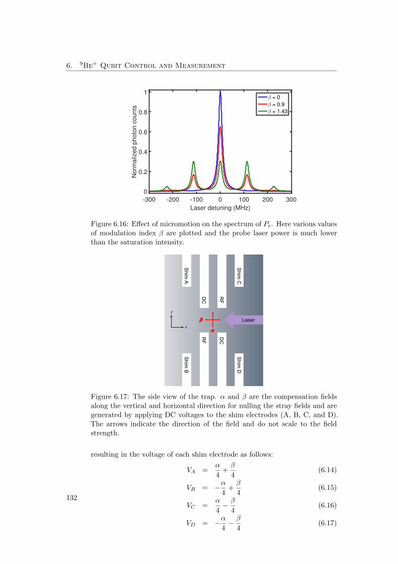
6. 9Be+ Qubit Control and Measurement
Laser detuning (MHz)
-300 -200 -100 0 100 200 300
Norm
aliz
ed p
hoto
n c
ounts
0
0.2
0.4
0.6
0.8
1β = 0
β = 0.9
β = 1.43
Figure 6.16: Effect of micromotion on the spectrum of Pe. Here various valuesof modulation index β are plotted and the probe laser power is much lowerthan the saturation intensity.
Sh
im A
S
him
B
Sh
im C
S
him
D
DC
RF
RF
DC
a
b
x
y
Laser
Figure 6.17: The side view of the trap. α and β are the compensation fieldsalong the vertical and horizontal direction for nulling the stray fields and aregenerated by applying DC voltages to the shim electrodes (A, B, C, and D).The arrows indicate the direction of the field and do not scale to the fieldstrength.
resulting in the voltage of each shim electrode as follows:
VA =α
4+β
4(6.14)
VB = −α4
+β
4(6.15)
VC =α
4− β
4(6.16)
VD = −α4− β
4(6.17)
132

6.6. Micromotion Compensation
It should be noticed that the field in the horizontal direction (β) is ten timesstronger than that in the vertical direction (α) due to the trap geometry.
Fluorescence Spectroscopy
Detection AOM frequency (MHz)
160 180 200 220 240
PM
T p
hoto
n c
ounts
0
10
20
30
40
Figure 6.18: The frequency scan of the detection beam. Three traces corre-sponds to different shim voltages used for micromotion compensation. TheRF drive frequency is ΩRF ≈ 2π × 110 MHz in this case. In the presence ofmicromotion, there is a sideband at the RF drive frequency. This AOM isin a double-pass setup so the frequency should be doubled. The blue traceshows that the micromotion is well compensated along the propagating direc-tion of the laser beam. The green trace indicates that the modulation indexis around 1.43 since the carrier and first micromotion sideband have nearlyequal strength.
The first method we tried is the use of fluorescence spectroscopy with thedetection beam, as shown in Fig. 6.18. The frequency of the detection beamis scanned using the AOM. Ideally we obtain a Lorentzian profile centered atthe atomic resonance as derived in Eq. (6.13) with β = 0. However in thepresence of micromotion we can see a sideband appeared at the RF drivingfrequency. Owing to the limited bandwidth of the AOM, we are not ableto observe higher-order micromotion sidebands. To null the stray fields, weapply voltages (α and β) on the shim electrodes, which generate compensationfields, while setting the laser frequency at the micromotion sideband untilthe sideband signal is minimized. This method is simple, but it can notguarantee that the ion is really at the center of the pseudopotential because
133

6. 9Be+ Qubit Control and Measurement
the micromotion is only minimized along the propagating direction of thedetection beam, which is at 45 with respect to the trap axis (see Fig. 5.2).For this method, one can fully compensate the stray fields using three laserbeams which are illuminated to the ion from three directions perpendicular toeach other, so each laser beam is sensitive to micromotion along its directionof propagation. However one axis is not accessible in our setup.
Micromotion Mapping
Offset: -300 meV
y (7
m)
-10
0
10
x (7m)-10 0 10
Offset: 0 meVy
(7m
)
-10
0
10
x (7m)-10 0 10
Offset: 330 meV
y (7
m)
-10
0
10
x (7m)-10 0 10
Offset: 700 meV
y (7
m)
-10
0
10
x (7m)-10 0 10
Offset: 1500 meV
y (7
m)
-10
0
10
x (7m)-10 0 10
Offset: 1900 meV
y (7
m)
-10
0
10
x (7m)-10 0 10
Figure 6.19: The simulated pseudopotential in the radial plane with differentDC potential offsets. It can be seen that the principal axes in the x − yplane are rotated depending on the DC potential offsets. This would affectthe micromotion as well as the efficiency of laser cooling.
In a 3-D segmented traps, it is possible to rotate the principal axes in theradial (x− y) plane by applying different static voltages to the DC electrodes(different DC potential offsets) [Madsen 06]. Normally the principal axes ofan ion trap are chosen for efficient laser cooling. If the laser wave vector khas a component along each of the three principal axes, it can cool ion’s threemotional modes. Figure 6.19 shows simulation results of the superimposedpseudo- and static potential in the radial plane for different DC potential off-sets. Here we keep the axial frequency constant and only the DC potentialoffset differs. As the radial principal axes are rotated, the shape and orien-
134

6.6. Micromotion Compensation
tation of the total potential changes. In the experiment, we observe thatthe required compensation field for minimizing the micromotion changes de-pending on the DC potential offsets, or equivalently the rotation of the radialprincipal axes. The measurement results for the 40Ca+ and 9Be+ ion areshown in Fig. 6.20. For each DC potential offset, we picked a range of valuesof α and performed a scan of β for each. Then we recorded the β value thatproduces the maximal fluorescence. It shows that there is a crossing pointamong different data sets. We think the α and β value at this point is theoptimal setting for micromotion compensation because it is independent ofthe tilt of the radial principal axes. Nevertheless, this mapping method onlyprovides information about micromotion along the direction of the detectionbeam.
Shim α
-10 -5 0 5 10
Shim
β
-10
-5
0
5
1015 meV
700 meV
-700 meV
328 meV
-300 meV
(a)
Shim α
-15 -10 -5 0
Shim
β
-6
-4
-2
0
2
4
6 6 meV
700 meV
-300 meV
149 meV
495 meV
-157 meV
(b)
Figure 6.20: Mapping of the compensation fields for different DC potentialoffsets (rotating the principal axes in the radial plane). (a) Work on a single40Ca+ ion. (b) A single 9Be+ ion.
RF Tickle
The last approach, which is also the most precise one, is the RF tickle tech-nique [Ibaraki 11]. The trap RF drive is amplitude modulated at ion’s secularfrequency. Once the ion is not at the RF null, this amplitude modulated RFfield can excite ion’s motion. This provides us a clean measurement that isindependent of the laser beam directions. The setup is illustrated in Fig. 6.21.The modulation signal starts from two DDS channels. The outputs from DDSsare mixed and then passed through a low-pass (LP) filter. The remaining sig-nal m(t) only contains the few-MHz secular frequency component. The RFsignal driving the trap is the carrier signal that is split into two paths witha power splitter (PS). The carrier signal in one path is multiplied with themodulation signal in a mixer, and then combined with the carrier signal from
135
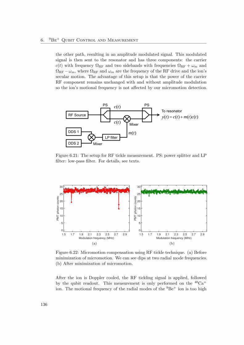
6. 9Be+ Qubit Control and Measurement
the other path, resulting in an amplitude modulated signal. This modulatedsignal is then sent to the resonator and has three components: the carrierc(t) with frequency ΩRF and two sidebands with frequencies ΩRF + ωm andΩRF−ωm, where ΩRF and ωm are the frequency of the RF drive and the ion’ssecular motion. The advantage of this setup is that the power of the carrierRF component remains unchanged with and without amplitude modulationso the ion’s motional frequency is not affected by our micromotion detection.
DDS 1
DDS 2
RF Source
LP filter
PS PS
Mixer
Mixer
To resonator ( )c t
( )m t
( ) ( ) ( ) ( )y t c t m t c t
( )c t
Figure 6.21: The setup for RF tickle measurement. PS: power splitter and LPfilter: low-pass filter. For details, see texts.
Modulation frequency (MHz)
1.5 1.7 1.9 2.1 2.3 2.5 2.7 2.9
PM
T p
hoto
n c
ounts
0
5
10
15
20
25
30
(a)
Modulation frequency (MHz)
1.5 1.7 1.9 2.1 2.3 2.5 2.7 2.9
PM
T p
hoto
n c
ounts
0
5
10
15
20
25
30
(b)
Figure 6.22: Micromotion compensation using RF tickle technique. (a) Beforeminimization of micromotion. We can see dips at two radial mode frequencies.(b) After minimization of micromotion.
After the ion is Doppler cooled, the RF tickling signal is applied, followedby the qubit readout. This measurement is only performed on the 40Ca+
ion. The motional frequency of the radial modes of the 9Be+ ion is too high
136

6.6. Micromotion Compensation
Strong
Weak
x
y
7 10
B A
C D
1.03
0.05 0.72
0.125
M
Figure 6.23: The summary of the RF tickle measurement. We draw a cartoonof the pseudopotential, which is tilted, and two principal axes of the radialconfinement for the ion. The α and β values for the points A, B, C, and D areobtained from the 2-D scan. From which, we can calculate the required voltagesettings (α and β) at the crossing point M, where ideally is the pseudopotentialminimum.
(∼ 10 MHz) such that the sidebands of the modulated signal would be filteredout by the resonator for which the half-power linewidth is around 1 MHz inour case. One the other hand, if we null the stray fields such that the calciumion is at the pseudopotential minimum, the beryllium should be the same. Wefirst perform a frequency scan without applying any compensation field. Thespectrum is shown in Fig. 6.22(a). There are two dips corresponding to themotional frequency of two radial modes. The next step is that we picked an αvalue and perform a 2-D scan in which the y axis is the β value and the x axisis the tickle frequency scanned over two radial modes2. For α = 7, it is foundthat β = −1.03 can make the micromotion vanish for the weak radial mode.This means the ion is either at the center of the pseudopotential or on theprincipal axis of the strong radial confinement. For the same α, making themicromotion vanish for the strong radial mode needs β = −0.05. Since two β
2Since when we change the shim voltage, the motional frequency of the ion slightly shifts.Therefore 2-D scan is needed in this measurement. For some technical reasons, the raw 2-Dscan data was not recorded by the computer so it can not be shown here. Only the screenshotpictures and notes were saved. These data shown were taken on 24.10.2014.
137

6. 9Be+ Qubit Control and Measurement
values are not the same, so we can conclude that in the first case the ion is onthe principal axis of the strong radial confinement while the weak radial modecan not be excited. In the latter one, the ion is on the principal axis of theweak radial confinement. Next, we chose the other α = 10 and followed thesame procedures. The results are summarized in Fig. 6.23 for clarification.We can determine a linear equation from two points on the principal axisof strong radial confinement and two points on the principal axis of weakradial confinement. The crossing point of these two linear equations will bethe pseudopotential minimum. After calculating α and β at the crossing pointand set them in the experiment, we repeated the RF tickle measurement again.We found the micromotion is well compensated, as shown in Fig. 6.22(b).
6.7 Conclusions
In this chapter we began with the loading procedure for the 9Be+ ions. Ba-sic techniques and calibrations required for 9Be+ qubit manipulations weredescribed. We demonstrated 9Be+ ion ground state cooling and created long-lived quantum memories using first-order magnetic-field-independent hyper-fine transitions. The results with 9Be+ qubits showed a coherence time of≈ 1.5 s. In principle, this coherence time can be further improved by finetuning the magnetic field to get the field-independent point and stabilizingthe Raman beam path better, for example we can cover the setup with a boxto suppress the influence from the environment.
The most severe problem we faced was the micromotion of the ion. Thestray fields in the trap can cause a variety of problems for quantum control oftrapped ions especially for mixed-species ion chains. For the intrinsic (axial)micromotion which can not be nulled with additional compensation fields, wemoved the ion along the axial direction trying to find a position where thistype of micromotion is minimum. However, there is no minimal point whereit is zero, probed with non-copropagating Raman beams (the wavevector dif-ference along the axial direction)3. The excess micromotion can be minimizedby applying voltages to shim electrodes which generate compensation fields.In our experiment, we tried three methods, in two of which we relied on thefluorescence detection. The minimization of micromotion is only along thepropagating direction of the probe field, which is at 45 with respect to theaxial direction. In this case, the ion is not at the pseudopotential minimumeven after we have maximal fluorescence counts. The lighter beryllium ion hasmuch larger axial micromotion than the heavier calcium ion. The intrinsic mi-cromotion always has a component projecting onto the propagating directionof the probe field. Consequently, to cancel out this vector projection of the
3Meanwhile, we also notice that the group at NIST also has strong axial micromotion inone of their traps. However they recently show that they can use the second micromotionsideband to perform high-fidelity quantum control of multiple qubits.
138

6.7. Conclusions
intrinsic micromotion on the probe field direction, different shim voltage set-tings are required for two ion species. It is quite hard for us to find a commonshim voltage setting for both ion species. If we use the shim voltage settingof the calcium ion, we lose the fluorescence from the readout of the berylliumion, and vice versa. The third method we used is the RF tickle. By amplitudemodulating the trap RF field and optimizing the shim voltage settings, wecould make the ion sit at the pseudopotential minimum. However, this opti-mal shim voltage setting does not reflect on the fluorescence detection of theberyllium ion due to the presence of intrinsic micromotion.
Our aim is to achieve high-fidelity control of two-species ion chains. Al-though the calcium and beryllium ions have not been operated together, thischapter combined with the characterizations for the calcium ion covered in[Kienzler 15b] provides the basic elements we need for control of both speciesof ions. Before writing the thesis, the beryllium ion system has been usedfor demonstrating the single-qubit transport gate for the first time. Thedetails will be presented in Ludwig de Clercq’s forthcoming Ph.D. thesis[de Clercq 15].
139

Chapter 7
Squeezed Schrodinger’s Cat States
The creation and study of nonclassical states of spin systems coupled to aharmonic oscillator has provided fundamental insights into the nature of de-coherence and the quantum-classical transition. These states and their con-trol form the basis of experimental developments in quantum informationprocessing and quantum metrology [Monroe 95a, Wineland 13, Haroche 13].Two of the most commonly considered states of the oscillator are squeezedstates and superpositions of coherent states of opposite phase, which are com-monly referred to as “Schrodinger’s cat” (SC) states. Squeezed states involvereduction of the fluctuations in one quadrature of the oscillator below theground state uncertainty, which has been used to increase sensitivity in in-terferometers [Collaboration 11, Aasi 13]. SC states provide a complemen-tary sensitivity to environmental influences by separating the two parts ofthe state by a large distance in phase space. These states have been cre-ated in microwave and optical cavities [Vlastakis 13, Haroche 13], where theyare typically not entangled with another system, and also with trapped ions[Monroe 96, McDonnell 07, Haljan 05a, Wineland 13], where all experimentsperformed have involved entanglement between the oscillator state and theinternal electronic states of the ion. SC states have recently been used as sen-sitive detectors for photon scattering recoil events at the single photon level[Hempel 13].
This Chapter presents our recent results in which we use a single trapped40Ca+ ion to combine for the first time highly squeezed states with superpo-sitions of distinct atomic wavepackets commonly referred to as Schrodinger’scat states. This work demonstrates direct measurements on the squeezed stateof the ion, revealing key features of the squeezed nature in phase space. Thecoherence of the squeezed Schrodinger’s cat states is verified by recombiningthe squeezed wavepackets, which we measure through the revival of the spincoherence. I will first review how to prepare the squeezed vacuum state of anion’s motion by reservoir engineering, a technique covered in more detail in the
141

7. Squeezed Schrodinger’s Cat States
thesis of Daniel Keinzler [Kienzler 15b]. Then the creation and measurementof the squeezed Schrodinger’s cat states will be presented. The results shownin this chapter are covered in our recent publications [Kienzler 15a, Lo 15].
7.1 Dissipative Quantum State Preparation
7.1.1 Reservoir Engineering
Reservoir engineering is a method in which specially designed couplings be-tween a system of interest and an environment, which is the vacuum modesof the electromagnetic field, can be used to generate quantum superpositionstates of the system as the steady state of the dissipative process. Follow-ing the proposals [Cirac 93a, Poyatos 96], we have developed techniques toprepare quantum harmonic states of a single trapped 40Ca+ ion, includingcoherent states, squeezed states and displaced-squeezed states [Kienzler 15a].Basically the process is implemented by introducing an artificial decay channelfor the spin states in form of an effective zero temperature reservoir, combinedwith engineered spin-oscillator couplings.
In the analysis, we consider the system shown in Fig. 7.1(a), where the ion’smotion is described by a quantum harmonic oscillator and the internal stateof the ion is restricted to a three-level system containing two long-lived qubitstates and one short-lived excited state. Two qubit states are denoted by|↑〉 and |↓〉 driven by laser fields with a Rabi frequency Ω, and the state |e〉represents the short-lived excited state of the ion with a spontaneous decayrate of γ. The state |↑〉 can couple to the state |e〉 by a laser field with acoupling strength (Rabi frequency) Ωe↑, generating an artificial decay channelfrom |↑〉 to |↓〉. The effective spontaneous emission rate for the state |↑〉 isgiven by γ↑ ≈ Ω2
e↑/γ [Haroche 06]. Here γ is supposed to be much larger thanthe emission rate from |e〉 to |↑〉 and the Rabi frequency Ωe↑. In the Lamb-Dicke regime, the effect of the photon recoil from the spontaneous emissionon the ion’s motional state can be neglected.
The dynamics of the whole system can be described by a master equation:
dρ
dt= − i
~
[H, ρ
]+ L(ρ) (7.1)
where ρ is the total density matrix for the ion and H the general spin-motioncoupling Hamiltonian, given by
H =~2
Ω(Kσ+ + K†σ−
)(7.2)
where σ+ = |↑〉 〈↓| and σ− = |↓〉 〈↑| are the spin flip operators and K (K†) isa general motional annihilation (creation) operator. The Louvillian operator
142

7.1. Dissipative Quantum State Preparation
Ion motion Internal states (a)
(b) Squeezed state preparation
Figure 7.1: (a) The system we consider for dissipative quantum state prepara-tion. (b) The transitions involved in the squeezed vacuum state preparation.The blue (red) motional sideband is marked with blue (red) arrows. The decayis labeled with dash lines. The steady state of the process is reached whenthe total probability amplitude of exciting the state |↑, n〉 from |↓, n− 1〉 and|↓, n+ 1〉 vanish.
L(ρ) describes the decay process with the form
L(ρ) = γ↑σ−ρσ+ −γ↑2
(ρσ+σ− + σ+σ−ρ) (7.3)
In general, solving this master equation is difficult and requires numericalcomputations. We only consider a limiting case in which γ↑ Ω the effectivequbit decay rate is much larger than the coupling strength. Therefore we canadiabatically eliminate the spin population in |↑〉. By introducing the partialmatrix elements of the density operator ρij = 〈i| ρ |j〉, where i, j ∈ ↑, ↓,the density matrix can be re-written as
ρ = ρ↓↓ |↓〉 〈↓|+ ρ↓↑ |↓〉 〈↑|+ ρ↑↓ |↑〉 〈↓|+ ρ↑↑ |↑〉 〈↑| (7.4)
These density operators ρij still act on the motional state of the ion. Insert-ing Eq. (7.4) into Eq. (7.1), we can obtain four evolution equations for ρij
143

7. Squeezed Schrodinger’s Cat States
[Haroche 06, Kienzler 15b]. After applying adiabatic elimination and somealgebraic simplification, the evolution equation for ρ↓↓ is
dρ↓↓dt
=Ω2
γ↑Kρ↓↓K
† − 1
2
Ω2
γ↑
(ρ↓↓K
†K + K†Kρ↓↓
)(7.5)
This shows that the evolution equation for the ion’s motion takes a Lindbladform with a decay rate of Ω2
γ↑. The Lindblad operator is expressed by L =
Ω√γ↑K. The ion’s motion undergoes relaxation processes until it reaches the
final state |ψ〉 satisfying L |ψ〉 = 0. This dissipative state preparation canbe easily understood in the resolved sideband cooling for which K = a isthe annihilation operator of the harmonic oscillator, resulting a Hamiltonianfor the red sideband drive. After several dissipative pumping cycles, the ioncan be cooled to its motional ground state (a |0〉 = 0). However this methodcan be extended to generate quantum superposition states of the harmonicoscillator by engineering the operator K [Kienzler 15a, Poyatos 96].
7.1.2 Squeezed Vacuum State Preparation
In the work on squeezed cats, we work with squeezed vacuum states. To obtainthese, we start with the relation a |0〉 = 0, where |0〉 is the ground state ofthe harmonic oscillator. Now we introduce an unitary operator U such thatU aU †U |0〉 = 0 is still valid. The state of interest is defined as |ψ〉 = U |0〉 andthe general motional annihilation operator becomes K = U aU †.
The squeezed vacuum state |ξ〉 is defined by the action of the squeezing oper-
ator S(ξ) = e(ξ∗a 2−ξa† 2)/2 on the motional ground state |0〉, where ξ = reiφs
with r and φs real parameters, which define the magnitude and the direc-tion of the squeezing in phase space. In order to generate squeezed vac-uum states as the desired state of the pumping process, we implement acoupling Hamiltonian of the form given in Eq. (7.2), with the operatorK = S(ξ)a S†(ξ) = cosh ra + eiφs sinh ra† . This requires simultaneous ap-plication of laser fields resonant with both the red motional sideband transi-tion (Hrsb = ~
2Ωr(σ+aeiφr + h.c.)) and the blue motional sideband transition
(Hbsb = ~2Ωb(σ+a
†eiφb+h.c.)). The ratio of the Rabi frequencies on these tran-
sitions gives the strength of the squeezing through r = tanh−1 ΩbΩr
while thephase is given by the phase difference between the two frequency componentsof the laser φs = φb − φr.
The squeezed state stabilization can also be understood as a quantum interfer-ence process. Figure 7.1(b) shows the ladder structure involved in the squeezedstate pumping process. The blue (red) motional sideband couples the states|↓, n− 1〉 (|↓, n+ 1〉) and |↑, n〉. The evolution stops when the total transitionprobability amplitude is zero. The following condition must be fulfilled:
cn−1 〈↑, n| Hbsb |↓, n− 1〉+ cn+1 〈↑, n| Hrsb |↓, n+ 1〉 = 0 (7.6)
144

7.2. Creation of Squeezed Schrodinger’s Cat States
Using the definitions of the Hamiltonian above, this condition can be simplifiedto
cn−1Ωb
√n+ cn+1Ωr
√n+ 1 = 0 (7.7)
There are two sets of solution, one contains only even phonon states and theother contains only odd phonon states. As we can see, only the even solutionincludes the ground state of the harmonic oscillator so this case is consid-ered here. Taking normalization into account, the solution of this recurrencerelation is [Gerry 05]
cn = c2m = (−1)m√
(2m)!
2mm!
(eiφs tanh r)m√cosh r
(7.8)
where r = tanh−1 ΩbΩr
, which is consistent with the one we obtained above.Therefore the squeezed vacuum state is
|ξ〉 =1√
cosh r
∞∑m=0
(−1)m√
(2m)!
2mm!eimφs(tanh r)m |2m〉 (7.9)
The probability distribution p(n) is now given by
p(n) = p(2m) = |〈2m| ξ〉|2 =(2m)!
22m(m!)2
(tanh r)2m
cosh r(7.10)
p(n) = p(2m+ 1) = 0 (7.11)
The probability vanishes for all odd n.
7.2 Creation of Squeezed Schrodinger’s Cat States
7.2.1 Theoretical Description
We use state-dependent forces (SDFs) to create superpositions of distinctsqueezed oscillator wavepackets which are entangled with a pseudo-spin en-coded in the electronic states of a single trapped ion. We will refer to thesestates as squeezed wavepacket entangled states (SWES) in the rest of thischapter.
A SDF is performed by simultaneously driving the red |↓〉 |n〉 ↔ |↑〉 |n− 1〉and blue |↓〉 |n〉 ↔ |↑〉 |n+ 1〉 motional sidebands of the spin flip transition[Monroe 96]. The resulting interaction Hamiltonian can be written in theLamb-Dicke approximation as
HD = ~Ω
2σx
(a† e−iφD/2 + a eiφD/2
), (7.12)
where Ω is the strength of the SDF, φD is the relative phase of the two lightfields, and σx ≡ |+〉 〈+| − |−〉 〈−| with |±〉 = (|↑〉 ± |↓〉)/
√2. For an ion
145

7. Squeezed Schrodinger’s Cat States
prepared in |+〉, this Hamiltonian results in displacement of the motional statein phase space by an amount α(τ) = −iΩe−iφD/2τ/2 which is given in unitsof the r.m.s. extent of the harmonic oscillator ground state. An ion preparedin |−〉 will be displaced by the same amount in the opposite direction. In thefollowing equations, we use α in place of α(τ) for simplicity. Starting fromthe state |↓〉 |ξ〉, application of the SDF ideally results in the SWES
|ψ(α)〉 =1√2
(|+〉 |α, ξ〉 − |−〉 |−α, ξ〉) , (7.13)
where we use the notation |α, ξ〉 = D(α)S(ξ) |0〉 with the displacement oper-
ator D(α) = eαa†−α∗a . A projective measurement of the spin performed in
the σz basis gives the probability of being |↓〉 as P (↓) = (1 + X)/2, whereX = 〈α, ξ| − α, ξ〉 = 〈−α, ξ|α, ξ〉 gives the overlap between the two displacedmotional states, which can be written as
X(α, ξ) = e−2|α|2(exp(2r) cos2(∆φ)+exp(−2r) sin2(∆φ)) (7.14)
where ∆φ = arg(α) − φs/2. When ∆φ = 0, the SDF is aligned with thesqueezed quadrature of the state, while for ∆φ = π/2, the SDF is aligned withthe anti-squeezed quadrature. At displacements for which X gives a measur-able signal, monitoring the spin population as a function of the force durationτ for different choices of ∆φ allows us to characterise the spatial variation ofthe initial squeezed wavepacket [Hao-Sheng 05, Gerritsma 10, Casanova 12].For values of |α|2 which are greater than the wavepacket variance along thedirection of the force, the state in Eq. (7.13) is a distinct superposition ofsqueezed wavepackets which have overlap close to zero and are entangled withthe internal state. For r = 0 (no squeezing) the state reduces to the famil-iar “Schrodinger’s cat” states which have been produced in previous work[Monroe 96, McDonnell 07, Haljan 05a, Wineland 13]. For r > 0 the super-posed oscillator states are the displaced-squeezed states [Caves 81, Yuen 76].
7.2.2 Experimental Details
The experiments make use of a segmented linear Paul trap with an ion-electrode distance of ≈ 185 µm. Motional heating rates from the groundstate for a 40Ca+ ion in this trap have been measured to be 10± 1 quanta/s,and the coherence time for the number state superposition (|0〉+ |1〉)/
√2 has
been measured to be 32± 3 ms [Kienzler 15b]. This experiment uses a singletrapped 40Ca+ ion, which mechanically oscillates on its axial vibrational modewith a frequency close to ωz/(2π) = 2.1 MHz. This mode is well resolved fromall other modes. The first step of each experimental run involves cooling allmodes of motion of the ion close to the Doppler limit using laser light at397 and 866 nm. We encode a pseudo-spin system in the internal electronicstates |↓〉 ≡
∣∣S1/2,MJ = 1/2⟩
and |↑〉 ≡∣∣D5/2,MJ = 3/2
⟩. This transition is
146

7.2. Creation of Squeezed Schrodinger’s Cat States
resolved by 200 MHz from all other internal state transitions in the appliedmagnetic field of 119.6 G. All coherent manipulations, including the squeezedstate preparation and the SDF, make use of the quadrupole transition betweenthese levels at 729 nm, with a Lamb-Dicke parameter of η ' 0.05 for the axialmode. This is small enough that the experiments are well described using theLamb-Dicke approximation [Wineland 98]. A discussion of this approximationis given in Chapter 7.2.4.
The state-dependent forces (SDFs) and the reservoir engineering in our exper-iment require the application of a bichromatic light field. We generate bothfrequency components using acousto-optic-modulators (AOMs) starting froma single laser stabilized to an ultra-high-finesse optical cavity with a resultinglinewidth < 600 Hz (at which point magnetic field fluctuations limit the qubitcoherence). We apply pulses of 729 nm laser light using a double-pass AOM towhich we apply a single radio-frequency tone, followed by a single-pass AOMto which two radio-frequency tones are applied. Following this second AOM,both frequency components are coupled into the same single-mode fiber beforedelivery to the ion. The double-pass AOM is used to switch on and off thelight. Optical pumping to |↓〉 is implemented using a combination of linearlypolarized light fields at 854 nm, 397 nm and 866 nm. The internal state of theion is read out by state-dependent fluorescence using laser fields at 397 nmand 866nm.
7.2.3 Experimental Results and Discussions
First Measurement
We apply the SDF directly after the squeezed vacuum state has been preparedby reservoir engineering and the internal state has been prepared in |↓〉 byoptical pumping (in the ideal case, the ion is already in the correct state andthis step has no effect). Figure 7.2 shows the results of measuring 〈σz〉 afterapplying displacements along the two principal axes of the squeezed statealongside the same measurement made using an ion prepared in the motionalground state. In order to extract relevant parameters regarding the SDF andthe squeezing, we fit the data using P (↓) = (A + BX(α, ξ))/2, where theparameters A and B account for experimental imperfections such as shot-to-shot magnetic field fluctuations (see Chapter 7.2.5 for discussions). Fittingthe ground state data with r fixed to zero allows us to extract Ω/(2π) =13.25± 0.40 kHz (here and in the rest of the paper, all errors are given ass.e.m.). We then fix this in performing independent fits to the squeezed-statedata for ∆φ = 0 and ∆φ = π/2. Each of these fits allows us to extractan estimate for the squeezing parameter r. For both the squeezed and anti-squeezed quadratures we obtain consistent values with a mean of r = 1.08 ±0.03, corresponding to 9.4 dB reduction in the squeezed quadrature variance.The inset shows the spin population as a function of the SDF phase φD with
147

7. Squeezed Schrodinger’s Cat States
P
X
a c b
0 20 40 60 80 100 1200.4
0.5
0.6
0.7
0.8
0.9
1
P(↓
)
SDF duration (µs)
0 100 200 3000.4
0.6
0.8
1
SDF phase (degree) P
(↓)
Ground state = /2 = 0
a
b
c
P
X
P
X
Figure 7.2: Spin-population evolution due to spin-motion entangle-ment. Projective measurement of the spin in the σz basis as a function ofSDF duration. a, Forces parallel to the squeezed quadrature (red triangles). b,An ion initially prepared in the motional ground state (blue circles). c, Forcesparallel to the anti-squeezed quadrature (green squares). The inset shows ascan of the phase of the SDF for an initial squeezed state with the force dura-tion fixed to 20 µs. Each data point is the result of > 300 repetitions of theexperimental sequence. The given error bars indicate one standard error ofthe mean, and are generated under the assumption that the dominant sourceof fluctuations is quantum projection noise.
the SDF duration fixed to 20 µs. This is also fitted using the same equationdescribed above, and we obtain r = 1.13± 0.03.
The loss of overlap between the two wavepackets indicates that a SWES hasbeen created. In order to verify that these states are coherent superpositions,we recombine the wavepackets by applying a second “return” SDF pulse forwhich the phase of both the red and blue sideband laser frequency componentsis shifted by π relative to the first. This reverses the direction of the forceapplied to the motional states for both the |+〉 and |−〉 spin states. In theideal case a state displaced to α(τ1) by a first SDF pulse of duration τ1 has
148

7.2. Creation of Squeezed Schrodinger’s Cat States
P
X
a b = 0 = /2
P
X
0 50 100 150 200 2500.4
0.5
0.6
0.7
0.8
0.9
1τ1 = 60 µs
|∆α| ≃ 4.99
120 µs
9.99
160 µs
13.3
200 µs
16.6
250 µs
20.8
0 50 100 150 2000.4
0.5
0.6
0.7
0.8
0.9
1τ1 = 60 µs
|∆α| ≃ 4.99
120 µs
9.99
P(↓
)
Recombined SDF duration (µs)
Figure 7.3: Revival of the spin coherence. Spin populations as a functionof the duration of the second SDF pulse with the spin phase shifted by πrelative to the first pulse. a, Forces parallel to the squeezed quadrature. b,Forces parallel to the anti-squeezed quadrature. In all cases an increase inthe spin population is seen at the time when the two motional states areoverlapped, which corresponds to the time τ1 used for the first SDF pulse.The value of τ1 and the corresponding |∆α| calculated from the measuredRabi frequency are written above the revival of each dataset. The fractionalerror on the mean of each of the estimated |∆α| is approximately 3%. Thesolid lines are fitted curves using the same form as using in the fits in Fig. 7.2with the overlap function X(δα, ξ). The obtained values of r are consistentwith the data in Fig. 7.2. The definition of error bars is the same as in Fig.7.2.
a final displacement of δα = α(τ1) − α(τ2) after the return pulse of durationτ2. For τ1 = τ2, δα = 0 and the measured probability of finding the spinstate in |↓〉 is 1. In the presence of decoherence and imperfect control, theprobability with which the ion returns to the |↓〉 state will be reduced. InFig. 7.3 we show revivals in the spin coherence for the same initial squeezedvacuum state as was used for the data in Fig. 7.2. The data include a rangeof different τ1. For the data where the force was applied along the squeezedaxis of the state (∆φ = 0), partial revival of the coherence is observed forSDF durations up to 250 µs. For τ1 = 250 µs the maximum separation ofthe two distinct oscillator wavepackets is |∆α| > 19, which is 56 times the
149

7. Squeezed Schrodinger’s Cat States
r.m.s width of the squeezed wavepacket in phase space. The amplitude ofrevival of this state is similar to what we observe when applying the SDFto a ground state cooled ion. The loss of coherence as a function of thedisplacement duration is consistent with the effects of magnetic-field inducedspin dephasing and motional heating [Turchette 00b, Hempel 13]. When theforce is applied along the anti-squeezed quadrature (∆φ = π/2), we observethat the strength of the revival decays more rapidly than for displacementswith ∆φ = 0. Simulations of the dynamics using a quantum Monte-Carlowavefunction approach including sampling over a magnetic field distributionindicate that this is caused by shot-to-shot fluctuations of the magnetic field(see Chapter 7.2.5).
Second Measurement
We are also able to monitor the number state distributions of the motionalwavepackets as a function of the duration of the SDF. This provides a sec-ond measurement of the parameters of the SDF and the initial squeezedwavepacket which has similarities with the homodyne measurement used inoptics [Breitenbach 97, Ourjoumtsev 07]. In order to do this, we opticallypump the spin state into |↓〉 after applying the SDF. This procedure destroysthe phase relationship between the two motional wavepackets, resulting inthe mixed oscillator state ρmixed = (|α, ξ〉 〈α, ξ|+ |−α, ξ〉 〈−α, ξ|) /2 (we esti-mate the photon recoil during optical pumping results in a reduction in thefidelity of our experimental state relative to ρmixed by < 3%, which wouldnot be observable in our measurements). The two parts of this mixture havethe same number state distribution, which is that of a displaced-squeezedstate [Caves 81, Yuen 76]. In order to extract this distribution, we drive Rabioscillations on the blue-sideband transition [Meekhof 96] and monitor the sub-sequent spin population in the σz basis. Figure 7.4 shows this evolution forSDF durations of τ = 0, 30, 60 and 120 µs. For τ = 30 and 60 µs, theresults from displacements applied parallel to the two principal axes of thesqueezed state are shown (∆φ = 0 and π/2). We obtain the number stateprobability distribution p(n) from the spin state population by fitting thedata using a form P (↓) = bt+ 1
2
∑n p(n)(1+e−γt cos(Ωn,n+1t)), where t is the
blue-sideband pulse duration, Ωn,n+1 is the Rabi frequency for the transitionbetween the |↓〉 |n〉 and |↑〉 |n+ 1〉 states and γ is a phenomenological decayparameter [Meekhof 96, Leibfried 03a]. The parameter b accounts for gradualpumping of population into the state |↑〉 |0〉 due to frequency noise on our laser[Di Fidio 00, Kienzler 15a]. It is negligible when p(0) is small. The resultingp(n) are then fitted using the theoretical form for the displaced-squeezed states(see Chapter 7.2.6). The number state distributions show a clear dependenceon the phase of the force, which is also reflected in the spin population evolu-tion. Figure shows the Mandel Q parameters of the experimentally obtainednumber state distributions, defined as Q = 〈(∆n)2〉/〈n〉 − 1 in which 〈(∆n)2〉
150

7.2. Creation of Squeezed Schrodinger’s Cat States
0 200 400 600 800 10000
0.2
0.4
0.6
0.8
1
P(↓
)
a
r = 1.08 ± 0.03
0 5 10 150
0.2
0.4
0.6
0.8
n
p(n
)
τ = 0 µs
0 200 400 600 800 10000
0.2
0.4
0.6
0.8
1
Blue sideband pulse duration (µs)
c
r = 1.03 ± 0.04, α = 1.09 ± 0.04
0 5 10 15 200
0.2
0.4
0.6
n
p(n
)
τ = 30 µs, ∆φ = π/2
0 200 400 600 800 10000
0.2
0.4
0.6
0.8
1
e
r = 1.05 ± 0.05, α = 2.12 ± 0.07
0 5 10 15 20 250
0.1
0.2
0.3
0.4
n
p(n
)
τ = 60 µs, ∆φ = π/2
0 200 400 600 800 10000
0.2
0.4
0.6
0.8
1
P(↓
)
b
r = 1.10 ± 0.06, α = 1.18 ± 0.02
0 5 10 150
0.1
0.2
0.3
0.4
n
p(n
)
τ = 30 µs, ∆φ = 0
0 200 400 600 800 10000
0.2
0.4
0.6
0.8
1
Blue sideband pulse duration (µs)
d
r = 1.03 ± 0.08, α = 2.38 ± 0.02
0 5 10 150
0.1
0.2
0.3
n
p(n
)
τ = 60 µs, ∆φ = 0
0 200 400 600 800 10000
0.2
0.4
0.6
0.8
1
f
r = 1.15 ± 0.29, α = 4.58 ± 0.04
0 5 10 15 20 25 300
0.1
0.2
0.3
n
p(n
)
τ = 120 µs, ∆φ = 0
Figure 7.4: Evolution of displaced-squeezed state mixtures. The ob-served blue-sideband oscillations and the corresponding number state proba-bility distributions for the SDF applied along the two principal axes of thesqueezed state and with different durations. a, Initial squeezed vacuum state.b, d, f, Forces parallel to the squeezed quadrature. c, e, Forces parallel tothe anti-squeezed quadrature. For τ = 30 µs the obtained parameters areconsistent within statistical errors. For τ = 60 µs the displacement along theanti-squeezed quadrature (e) results in a large spread in the number stateprobability distribution, with the result that in the fitting r and α are pos-itively correlated - the errors stated do not take account of this. We thinkthat this accounts for the apparent discrepancy between the values of r andα obtained for τ = 60 µs. The green-dashed line in the inset of d and f is thePoisson distribution for the same 〈n〉 as the created displaced-squeezed statemixture, which is given by 〈n〉 = |α|2 + sinh2r [Caves 81]. Each data pointis the average of 500 repeats of the experimental sequence. The definition oferror bars is the same as in Fig. 7.2.
and 〈n〉 are the variance and mean of p(n) respectively [Mandel 79]. The solidlines are the theoretical curves given by Caves [Caves 81] for r = 1.08, and arein agreement with our experimental results. For displacements along the shortaxis of the squeezed state (Fig. 7.4), the collapse and revival behaviour of thetime evolution of P (↓) is reminiscent of the Jaynes-Cummings Hamiltonianapplied to a coherent state [Haroche 06], but it exhibits a higher number ofoscillations before the “collapse” for a state of the same 〈n〉. This is surprisingsince the statistics of the state is not sub-Poissonian. We attribute this to thefact that this distribution is more peaked than that of a coherent state with
151

7. Squeezed Schrodinger’s Cat States
the same 〈n〉, which is obvious when the two distributions are plotted over oneanother (Figs. 7.4(d) and 7.4(f)). The increased variance of the squeezed statethen arises from the extra populations at high n, which are too small to makea visible contribution to the Rabi oscillations. For the squeezing parameter inour experiments sub-Poissonian statistics would only be observed for |α| > 3.For τ = 120 µs we obtain a consistent value of r and |α| = 4.6 only in thecase where we include a fit parameter for scaling of the theoretical probabilitydistribution, obtaining a fitted scaling of 0.81± 0.10 (see Chapter 7.2.6). Thereconstruction of the number state distribution is incomplete, since we cannotextract populations with n > 29 due to frequency crowding in the
√n+ 1 de-
pendence of the Jaynes-Cummings dynamics. As a result, we do not includethese results in Fig. . Measurement techniques made in a squeezed-state basis[Kienzler 15a] could avoid this problem, however these are beyond our currentexperimental capabilities for states of this size.
0 0.5 1 1.5 2 2.5 3 3.5−1
0
2
4
6
8
Q p
aram
eter
|α|
Figure 7.5: Mandel Q parameter for the displaced-squeezed states.Shown are the results for displacements along the squeezed quadrature (redtriangles) and the anti-squeezed quadrature (green squares). All the valuesare calculated from the experimental data given in Fig. 7.4, taking the prop-agation of error into account. The solid lines are theoretical curves for dis-placements along the squeezed (red) and anti-squeezed (green) quadraturesof an initial state with r = 1.08. The values of |α| are obtained from fits tothe respective p(n) (Fig. 7.4), with error bars comparable to the size of thesymbol. The point at |α| = 0 is the squeezed vacuum state.
7.2.4 Validity of Lamb-Dicke Approximation
The 729 nm laser beam enters the trap at 45 degrees to the z axis of the trapresulting in a Lamb-Dicke parameter of η ' 0.05 for the axial mode. For
152

7.2. Creation of Squeezed Schrodinger’s Cat States
Re(α)
Im(α
)
a
τ = 60 µs
−10 −5 0 5 10
−10
−5
0
5
100
0.02
0.04
0.06
0.08
Re(α)
c
τ = 120 µs
−10 −5 0 5 10
−10
−5
0
5
100
0.02
0.04
0.06
0.08
Re(α)
e
τ = 250 µs
−10 −5 0 5 10
−10
−5
0
5
100
0.02
0.04
0.06
0.08
Re(α)
Im(α
)
b
τ = 60 µs
−10 −5 0 5 10
−10
−5
0
5
100
0.02
0.04
0.06
0.08
Re(α)
d
τ = 120 µs
−10 −5 0 5 10
−10
−5
0
5
100
0.02
0.04
0.06
0.08
Re(α)
f
τ = 250 µs
−10 −5 0 5 10
−10
−5
0
5
100
0.02
0.04
0.06
0.08
Figure 7.6: Quasi-probability distributions for displaced-squeezedstates in phase space using LDA and non-LDA: a, c, e, The simu-lation results using LDA with different SDF durations. b, d, f, The resultssimulated using the full Hamiltonian.
this Lamb-Dicke parameter, we have verified whether for displacements up to|α| = 9.75 the dynamics can be well described with the Lamb-Dicke Approx-imation (LDA). We simulate the wavepacket dynamics using the interactionHamiltonian with and without LDA. In the simulation, we apply the SDF toan ion prepared in |↓〉 |ξ〉. The interaction Hamiltonian for a single trappedion coupled to a single-frequency laser field can be written as [Leibfried 03a]
HI =~2
Ω0σ+expiη(a e−iωzt + a† eiωzt)ei(φ−δt) + h.c.,
where Ω0 is the interaction strength, σ+ = |↑〉 〈↓|, a and a† are motionalannihilation and creation operators, ωz is the vibrational frequency of theion, φ is the phase of the laser, and δ = ωl − ωa the detuning of the laserfrom the atomic transition. In the laboratory, the application of the SDFinvolves simultaneously driving both the blue and red sideband transitionsresonantly resulting in the Hamiltonian Htot = Hbsb + Hrsb, where δ = ωz inHbsb and δ = −ωz in Hrsb. Starting from |↓〉 |ξ〉, the evolution of the state cannot be solved analytically. We perform a numerical simulation in which weretain only the resonant terms in the Hamiltonian. Figure 7.6 shows the quasi-probability distributions in phase space for chosen values of the SDF durationτ . These are compared to results obtained using the LDA. For τ = 60 µs bothcases are similar, resulting in |α| ' 2.4. For τ = 250 µs the squeezed statewavepackets are slightly distorted and the displacement is 4 % smaller for the
153
7. Squeezed Schrodinger’s Cat States
full simulation than for the LDA form. Considering the levels of error arisingfrom imperfect control and decoherence for forces of this duration, we do notconsider this effect to be significant in our experiments.
7.2.5 Simulations for the Coherence of Squeezed Cats
After creating SWESs, we deduce that coherence is retained throughout thecreation of the state by applying a second SDF pulse to the ion, which re-combines the two separated wavepackets and disentangles the spin from themotion. The revival in the spin coherence is not perfect due to decoherenceand imperfect control in the experiment. One dominant source causing deco-herence of the superpositions is spin decoherence due to magnetic field fluctua-tions. We have performed quantum Monte-Carlo wavefunction simulations toinvestigate the coherence of the SWES in the presence of such a decoherencemechanism. We simulate the effect of a sinusoidal fluctuation of the magneticfield on a timescale long compared to the duration of the coherent control se-quence, which is consistent with the noise which we observe on our magneticfield coil supply and from ambient fluctuations due to electronics equipmentin the room. The amplitude of these fluctuations is set to ' 2.2 mG, givingrise to the spin coherence time of ≈ 180 µs which we have measured usingRamsey experiments on the spin alone. Since the frequency of fluctuationsis slow compared to the sequence length, we fix the field for each run of thesimulation, but sample its value from a probability distribution derived froma sinusoidal oscillation. In Fig. 7.7 we show the effect of a single shot takenat a fixed qubit-oscillator detuning of 1.5 kHz, while in Fig. 7.8 we show theaverage over the distribution. In both figures results are shown for the SDFapplied along the two principal axes of the squeezed vacuum state as well asfor the motional ground state using force durations of 60 and 120 µs. We alsoshow the results of applying the second SDF pulse resulting in partial revivalof the spin coherence. It can be clearly seen that when the SDF is appliedalong the anti-squeezed quadrature, the strength of the revival decays morerapidly, and P (↓) oscillates around 0.5. This effect can be seen in the datashown in Fig. 7.3.
7.2.6 Number State Probability Distributions for the Displaced-Squeezed State
For Fig. 7.4, we characterize the probability distribution for the number statesof the oscillator. This is performed by driving the blue-sideband transition|↓〉 |n〉 ↔ |↑〉 |n+ 1〉 and fitting the obtained spin population evolution using
P (↓) = bt+1
2
∑n
p(n)(1 + e−γt cos(Ωn,n+1t)), (7.15)
154

7.2. Creation of Squeezed Schrodinger’s Cat States
0 20 40 600.4
0.6
0.8
1
P(↓
)
a
0 20 40 600.4
0.6
0.8
1
0 30 60 90 1200.4
0.6
0.8
1
SDF duration (µs)
P(↓
)
b
0 30 60 90 1200.4
0.6
0.8
1
Recombined SDF duration (µs)
Figure 7.7: Coherence of cat states with fixed magnetic field noise:The magnetic-field-induced energy-level-shift of 1.5 kHz is used in this simu-lation. a, The duration of both SDF pulses is 60 µs. b, The duration of bothSDF pulses is 120 µs. Red-dashed and green-dash-dot curves show the SDFaligned along the squeezed and anti-squeezed quadratures. The blue trace isfor the SDF applied to a ground state cooled ion.
where t is the blue-sideband pulse duration, p(n) are the number state probabil-ities for the motional state we concern, and γ is an empirical decay parameter[Meekhof 96, Leibfried 03a]. In the results presented here we do not scale thisdecay parameter with n as was done by [Meekhof 96]. We have also fittedthe data including such a scaling and see consistent results. The Rabi fre-quency coupling |↓〉 |n〉 to |↑〉 |n+ 1〉 is Ωn,n+1 = Ω0| 〈n| eiη(a†+a ) |n+ 1〉 | =
Ω0e−η2/2ηL1
n(η2)/√n+ 1. For small n, this scales as
√n+ 1, but since the
states include significant populations at higher n we use the complete formincluding the generalized Laguerre polynomial L1
n(x). The parameter b in thefirst term accounts for a gradual pumping of population into the state |↑〉 |0〉which is not involved in the dynamics of the blue-sideband pulse [Di Fidio 00,Kienzler 15a]. This effect is negligible when p(0) is small.
After extracting p(n) from P (↓), we fit it using the number state probability
155

7. Squeezed Schrodinger’s Cat States
0 20 40 600.4
0.6
0.8
1 P
(↓)
a
0 20 40 600.4
0.6
0.8
1
0 30 60 90 1200.4
0.6
0.8
1
SDF duration (µs)
P(↓
)
b
0 30 60 90 1200.4
0.6
0.8
1
Recombined SDF duration (µs)
Figure 7.8: Coherence of cat states with a magnetic field fluctuationdistribution: Assuming the magnetic field exhibits a 50-Hz sinusoidal pat-tern with an amplitude of 2.2 mG, this plot shows the simulation results bytaking an average over 100 samples on the field distribution. a, The durationof both SDF pulses is 60 µs. b, The duration of both SDF pulses is 120 µs.Definitions of the curve specification are the same as Fig. 7.7.
distribution for the displaced-squeezed state [Gerry 05],
p(n) = κ(1
2tanh r)n
n! cosh rexp
[−|α|2 − 1
2(α∗2eiφs + α2e−iφs) tanh r
]×∣∣∣∣Hn
[α cosh r + α∗eiφssinh r√
eiφs sinh 2r
]∣∣∣∣2where κ is a constant which accounts for the infidelity of the state duringthe application of SDF and the Hn(x) are the Hermite polynomials. Thedirection of the SDF is aligned along either the squeezing quadrature or theanti-squeezing quadrature of the state. Therefore, we set arg(α) = 0 and fixφs = 0 and π for fitting the data of the short axis and the long axis of thesqueezed state, respectively. This allows us to obtain the values of r and |α|for the state we created. For the cases of smaller displacements (from Figs.7.4(a) to (e)), we set κ = 1. For the data set of |α| ' 4.6 (Fig. 7.4(f)), κ isa fitting parameter which gives us a value of 0.81± 0.1. We note that in thiscase 4 % of the expected population lies above n = 29 but we are not able toextract these populations from our data.
156

7.2. Creation of Squeezed Schrodinger’s Cat States
The Mandel Q parameter [Mandel 79], defined as
Q =〈(∆n)2〉 − 〈n〉
〈n〉.
where 〈n〉 and 〈(∆n)2〉 are the mean and variance of the probability distri-bution. For a displaced-squeezed state these are given by Caves [Caves 81]as
〈(∆n)2〉 =∣∣∣α cosh r − α∗eiφssinh r
∣∣∣2 + 2 cosh2r sinh2r,
〈n〉 = |α|2 + sinh2r.
These forms were used to produce the curves given in Fig. 7.5.
7.2.7 Possible Applications
∆𝜃
P
X
a
X X
P P
b P
X X X
P P
∆𝜃
After 1st SDF pulse Phase shift
induced by noise
Apply 2nd SDF pulse
Figure 7.9: Possible application of using SWESs for interferometry: a,Use of squeezed state wavepackets. b, Use of ground state wavepackets. Thefirst SDF pulse is used to create a spin-motion entangled state. In the middle,a small phase shift ∆θ is induced by shot-to-shot fluctuation in the oscillatorfrequency before the application of the second SDF pulse, which recombinesthe two distinct oscillator wavepackets.
157

7. Squeezed Schrodinger’s Cat States
These novel states present new possibilities both for metrology and for con-tinuous variable quantum information. For the sensitive measurements, anexample is illustrated in Fig. 7.9 where we compare an interferometry experi-ment involving the use of a SWES versus a more standard Schrodinger’s catstate based on coherent states. In both cases the superposed states have aseparation of |2α| obtained using a SDF. For the SWES this force is alignedalong the squeezed quadrature of the state. The interferometer is closed byinverting the initial SDF, resulting in a residual displacement which in theideal case is zero. One form of noise involves a shot-to-shot fluctuations inthe oscillator frequency. On each run of the experiment, this would result in asmall phase shift ∆θ arising between the two superposed motional states. Asa result, after the application of the second SDF pulse the residual displace-ment would be αR = 2iα sin(∆θ/2), which corresponds to the states beingseparated along the P axis in the rotating-frame phase space. The final stateof the system would then be |ψ(αR)〉 with a corresponding state overlap givenby X(αR, ξ). Therefore the contrast will be higher for the SWES (Fig. 7.9(a))than for the coherent Schrodinger’s cat state (Fig. 7.9(b)) by a factor
exp[−2 |αR|2 (e−2r − 1)
].
While in our experiments other sources of noise dominate, in other systemssuch oscillator dephasing may be more significant.
In quantum information with continuous variables, the computational basisstates are distinguishable because they are separated in phase space by |∆α|and thus do not overlap [Weedbrook 12, Gottesman 01, Bartlett 02]. The deco-herence times of such superpositions typically scale as 1/|∆α|2 [Turchette 00b].The use of states squeezed along the displacement direction reduces the re-quired displacement for a given overlap by er, increasing the resulting coher-ence time by e2r which is a factor of 9 in our experiments. We therefore expectthese states to open up new possibilities for quantum state engineering andcontrol.
158

Chapter 8
Summary and Outlook
8.1 Summary
This thesis described work towards development of a system for investigationsof quantum information science with two species of ion. In close collaborationwith Daniel Kienzler and Ben Keitch, the ion trap, optics and computer con-trol systems were set up. A number of theoretical studies and experimentalcharacterizations of beryllium ions were performed. Quantum states of motionsuch as coherent states, squeezed states, and displaced-squeezed states havebeen generated by a new method [Kienzler 15a, Kienzler 15b], and also entan-glement of the spin and squeezed motion of a single ion have been created[Lo 15]. Both experiments were carried out with a single calcium ion.
The initial step of all the experiments is the design, setup, calibration, andcharacterization. The major concern of the trapped-ion quantum processoris the scalability. How to increase the number of qubits while maintain-ing high-fidelity control of them has drawn many research groups’ attention.The architecture for a large-scale ion-trap quantum computer [Kielpinski 02,Wineland 98] requires linear ion crystals which are composed of two ion speciesand moved in segmented trap arrays. Our segmented trap was designedtowards this goal, where there are three experimental zones, two zones forsplitting/combining/transporting ions, and two zones for loading (Chapter 4).Other new features were added to our trap design, for example the segmentedshim electrodes are used in order to compensate the stray fields in differentregions of the trap. The imaging system was also designed for monitoring anddetecting two ion species simultaneously that increases the flexibility for thecomplex experiments, for example two ion species gates or quantum simulationof an open quantum system.
We also constructed and characterized all-solid-state continuous-wave lasersystems for photoionization loading, cooling and quantum state manipulationof beryllium ions [Lo 14]. The wavelength required for photoionization of
159

8. Summary and Outlook
neutral beryllium atoms (235 nm) is created by two stages of second-harmonicgeneration (SHG) using PPKTP and BBO nonlinear crystals placed insideresonant cavities. In the first stage, we have demonstrated stable generationof 400 mW at 470 nm starting from 560 mW at 940 nm. In the second stage,with 140 mW input to the cavity, an output power of 28 mW at 235 nm isobtained. For quantum control of beryllium ions, three laser wavelengthsat 313 nm are produced by sum-frequency generation and subsequent SHG,starting from four infrared fiber lasers. Up to 7.2 W at 626 nm have beengenerated from 8.5 W at 1051 nm and 8.3 W at 1551 nm. The red light is thenfrequency-doubled in bowtie cavities using BBO crystals. With an incidentpower of 3.8 W, we obtain 1.9 W of UV light at 313 nm, which may help inthe long-term goal of fault-tolerant quantum computation using stimulatedRaman transitions because the difficulties derived from the trade-off betweenspontaneous scattering and quantum-gate speed can be overcome with high-intensity laser beams.
For the characterization of ions, most of the calcium part have been coveredin [Kienzler 15b]. In this thesis, we performed some diagnostic experimentsfor the beryllium ion. First, the readout error was analyzed by performingthe Rabi flops on different qubit states. We found that a high readout fidelitycan be achieved with shelving the dark state ion to another “darker” state.Second, the optical pumping efficiency was optimized and compared with thetheoretical predictions. Third, with an axial vibrational frequency of 2.7 MHzwe found that 98 % ground state preparation (〈n〉 = 0.02) after optimizationof the resolved sideband cooling can be achieved. Fourth, we performed theRamsey experiment to examine the coherence of the qubit. For the magnetic-field-sensitive qubit, the coherence time is approximately 105 µs without anymagnetic field stabilization. A coherence time of ≈ 1.5 s was observed for thefield-independent qubit. These results provide a basis for future work withmultiple ions.
The main problem we had was the micromotion of the ion. For controlling amixed-species ion chain, the micromotion compensation is an important task.We use different techniques to minimize the micromotion for both calcium andberyllium ions and to understand its behavior in our trap. Because calciumand beryllium ion have different intrinsic micromotion amplitude, it is notpossible to use the same shim voltage setting to minimize their micromotionalong the direction of the probe field, which is at 45 with respect to theaxial direction. Using the RF tickle method, we could find an optimal shimvoltage setting for the calcium ion. Under this situation, the calcium ionshould be at the pseudopotential minimum. However, this optimal settingis not for beryllium fluorescence detection due to the projection of intrinsicmicromotion on the probe field direction.
The calcium ion has lower intrinsic micromotion, which does not influence
160

8.2. Outlook
the fluorescence detection too much, so we just need to minimize the excessmicromotion by applying additional compensation fields. The main resultcovered in this thesis is the generation of squeezed Schrodinger’s cat states.This novel quantum state is created for the first time. These relied on newlydeveloped techniques, dissipative quantum state preparation. Artificial dissi-pation for the qubit is introduced to create an efficient irreversible dampingchannel for the ion’s energy. By engineering the spin-oscillator coupling, thisresults in effective relaxation of the motional state of the ion. This engi-neered damping processes keep the final state, which is the steady state of thedynamics, protected from other unwanted relaxation mechanisms. Using thistechnique we were able to prepare the coherent, the squeezed vacuum, and thedisplaced-squeezed states for an ion’s motion. This toolbox for generating andprotecting quantum harmonic oscillator states is transferrable to any physicalsystem and may facilitate quantum computation with continuous variables[Gottesman 01].
In the second experiment based on the previous one, we demonstrated superpo-sitions composed of squeezed wavepackets, which we generated by applying aninternal-state dependent force to a single trapped ion initialized in a squeezedvacuum state with 9 dB reduction in the quadrature variance. This allowedus to characterize the initial squeezed wavepacket by monitoring the onset ofspin-motion entanglement, and to verify the evolution of the number statesof the oscillator as a function of the duration of the force. In both cases, weobserved clear differences between displacements aligned with the squeezedand anti-squeezed axes. We observed coherent revivals when inverting thestate-dependent force after separating the wavepackets by more than 19 timesthe ground state root-mean-square extent, which corresponds to 56 times ther.m.s. extent of the squeezed wavepacket along the displacement direction.Aside from their fundamental nature, these states may be useful for quantummetrology [Munro 02], quantum state engineering, or quantum informationprocessing [Weedbrook 12, Gottesman 01, Bartlett 02] in a new regime.
8.2 Outlook
Using the system that has been built, there are still plenty of interestingexperiments we can do. Here some ongoing and upcoming experiments arelisted:
The first one is the transport gate [Leibfried 07]. Typically quantum gate oper-ations are implemented by shining laser pulses to the ions, which are staticallyin space. The other way around, one can also keep the laser on at certain placeand transport the ions through it. For a large-scale trapped-ion quantum pro-cessor, a big advantage of the transport gate scheme is that the complexity ofthe laser systems could be significantly reduced. It may also allow for efficient
161
8. Summary and Outlook
use of one and the same laser beam in many parallel operations. Recently, wedemonstrated single-qubit gate operations as well as the Ramsey experimentusing transported calcium and beryllium ions individually [de Clercq 15]. Thetwo-qubit transport gates will be the next.
The second experiment we will pursue is relevant to quantum simulation ofan open quantum system. In the beginning we will start from a small-scalequantum system, consisting of one beryllium ion and one calcium ion. Thequantum system is provided by the internal degree of freedom of berylliumion which we will couple to the motional degree of freedom represent theenvironment, continuously damped the calcium ion. The motional degree offreedom of beryllium ion is controlled by the calcium ion because the motionalstates of two ions in the same trap are shared. For quantum simulations,the ability to scatter photons from one “environment” ion (calcium) whilepreserving internal states of the other “system” ion (beryllium) may allow usto engineer controlled environments consisting of either the shared motionalstates, or of the internal states of the “environment” ion species.
One possibility is to continuously cool the calcium ion, and simultaneouslycouple the beryllium to the motion using either a Mølmer-Sørensen type cou-pling or a Jaynes-Cummings interaction. This should lead to decoherence ofa qubit stored in the beryllium ion. The idea here is that we should be ableto vary the cooling (damping) rate of the environment and the coupling of theberyllium ion to this environment in order to observe the transition betweenMarkovian and non-Markovian quantum dynamics. This means that one isable to control the information flow between the system and the environment.If the damping rate of the motional mode is made much smaller than thecoupling rate, the open quantum system will be in the non-Markovian regime,meaning that the motion remembers the ion coupling to the quantum system.By contrast, if the damping rate of the motional mode is larger than the cou-pling rate, it induces Markovian processes in which the motion rapidly losesinformation about the system-environment interaction. Many measures forthe degree of non-Markovian behavior of quantum processes in open systemshave been proposed [Wolf 08, Breuer 09, Rivas 10]. In our case, we still haveto investigate in detail how to measure the degree of non-Markovianity for theberyllium spin.
The same techniques used in this experiment could be applied to an implemen-tation of two-qubit gates using different atomic species [Ballance 15]. Perform-ing an entangling gate on two species of ions is of interest for several reasons.For trapped ion quantum repeaters made up of communication qubits andmemory qubits, the entanglement between the communication qubits fromtwo separate registers are created via the photonic channel, and then thequantum information within the communication qubits is coherently mappedto the memory qubits using standard entangling gate operations [Monroe 13].
162

8.2. Outlook
However, the communication qubits need to be well isolated from the mem-ory qubits because the scattering light from the excitation laser acting onthe communication qubits might destroy the information stored in memoryqubits. The best solution might be to use two different ion species to avoidthe crosstalk. Even for quantum computation which does not necessarily re-quire remote entanglement, the two species quantum gates are still useful inthe error correction codes, where we need entanglement between the primaryqubit with ancilla qubits, which are then measured by state-dependent fluores-cence [Chiaverini 04]. For the same concern, the scattering light or the emittedphotons when performing the measurement on the ancilla qubits might disturbthe primary qubit. Therefore, using two atomic species can benefit the fidelityof quantum operations.
The third future experiment is to measure the Wigner function of Schrodinger’scat states. So far all experiments on Schrodinger’s cat states performed us-ing trapped ions have involved entanglement between the oscillator state andthe internal electronic states of the ion. The wavefunction has the form of|ψ〉 = 1√
2(|+〉 |α〉 − |−〉 |−α〉), where |±〉 are the eigenstates of σx Pauli ma-
trix, and |±α〉 are the coherent states displaced to different directions. Inorder to observe interference fringes characteristic of a quantum superpositionin the Wigner tomography [Deleglise 08, Vlastakis 13], the wavefunction writ-ten in the σz basis is |ψ〉 = 1
2 [|↑〉 (|α〉 − |−α〉) + |↓〉 (|α〉+ |−α〉)]. In principle,we can decouple the motion from the spin by measurement. When we performa projective measurement on |↓〉, depending on whether we detect photons ornot we know the corresponding cat state. We can post select the events with-out photon scattering, which means the cat is still alive, and then perform thestate tomography to reconstruct the Wigner function for the motional state.
The fourth experiment we plan to perform would be the use of a single beryl-lium ion “qubit” interacting with an environment of calcium spins, whichwith appropriate couplings could realize a spin-bath model [Prokofiev 00]. Al-ternatively, interactions between the beryllium qubit and multiple motionalmodes may be used to realize spin-boson physics [Porras 08]. Other areas ofinvestigation include the use of engineered environments for quantum state en-gineering, for example multi-mode squeezed state preparation [Kienzler 15b]and stabilizing Schrodinger’s cat states [de Matos Filho 96, Roy 15].
163


Appendix A
Matrix Elements for theElectric-Quadrupole Interaction
As mentioned in Chapter 2.2, here shows the starting point how to obtain thematrix elements for the electric-quadrupole interaction. The (I ·J)2 term inEq. (2.4) can be simplified as
(I ·J)2 = (IzJz)2 +
1
2(IzJz)(I+J− + I−J+) +
1
2(I+J− + I−J+)(IzJz)
+1
4(I+J−)2 +
1
4(I−J+)4 +
1
4(I+I−J−J+) +
1
4(I−I+J+J−)
To calculate the matrix elements, one can use the following relations
J±|J mJ〉 = ~√
(J ±mJ + 1)(J ∓mJ)|J mJ ± 1〉I±|I mI〉 = ~
√(I ±mI + 1)(I ∓mI)|I mI ± 1〉
165


Appendix B
Lens Data
Table B.1: The data of the lenses in the imaging system are provided. d isthe distance from the current surface to the next one.
Surface number Radius of curvature (mm) d 313 nm path (mm) d 397 nm path (mm)
Object (ion) Inf 30.918 30.9181 Inf 5.985 5.9852 -60.491 9.4 9.43 -29.501 0.223 0.2234 -128.613 3.35 3.355 Inf 2.298 2.2986 -117.496 7.2 7.27 -56.446 0.339 0.3398 -290.973 6.25 6.259 -80.576 0.966 0.96610 311.817 14 1411 -118.789 0.5 0.512 Inf 42.038 42.03813 Inf 6.35 6.3514 Inf 650.602 697.49515 -13.333 3 8.816 -19.66 30.398 60.21117 11.657 6.6 6.618 9.934 180.751 98.244
Image (camera or PMT) Inf
167

B. Lens Data
1 2
3 12
Surface number:
15 16 17
13 14
18
Beryllium path
Calcium path
15 16 17 18
10 11
In-vacuum Objective vacuum
viewport
Figure B.1: The lens layouts. The in-vacuum objective is common for beryl-lium (313 nm) and calcium (397 nm) ions. Outside the vacuum, there is onelens pair in each path.
168

Appendix C
Second-Harmonic-GenerationEfficiency
Here we give the expressions used for the theoretical calculation of the second-harmonic-generation efficiencies plotted in Figs. 5.4, 5.6 and 5.12. The valuesfor the relevant parameters are given in Table C.1.
We start from the original equations from Boyd and Kleinman [Boyd 68] andrearrange them to formulate the conversion efficiency (in SI units [Risk 03])as
Γeff =P2ω
P 2ω
=16π2d2
eff
λ3ε0cnωn2ωlce−(βω+
β2ω2lc)× h(b, lc, βω, β2ω, σ, B) (C.1)
Here, P2ω is the SHG power and Pω the power in the fundamental wavelengthat the crystal (the circulating power if a cavity is used); deff is an effectivenon-linear coefficient in units of m ·V−1 (related but not identical to parame-ter d in [Boyd 68]); ε0 and c are the vacuum permittivity and speed of light,respectively; λ is the pump wavelength, lc the crystal length, βω (β2ω) the ab-sorption coefficient of the fundamental (second harmonic) light in the crystal,and nω (n2ω) the refractive index of the crystal sampled by the light in thefundamental (second harmonic) wavelength.
h is a dimensionless function which depends on lc, βω, β2ω, the confocal param-eter b = 2πnωw
2/λ (where w is the waist radius of the pump beam, assumedto be at the center of the crystal), the wavevector mismatch σ (scaled by b)and the walk-off parameter B = ρ(θ, λ)
√πlcnω/(2λ) where θ is the phase-
matching angle and
ρ(θ, λ) = arctan
1−(no,2ω
ne,2ω
)2
cot θ +(no,2ω
ne,2ω
)2tan θ
(C.2)
169

C. Second-Harmonic-Generation Efficiency
no,2ω (ne,2ω) is the refractive index for the second-harmonic light along theordinary (extraordinary) crystal axis.
The explicit expression for h is,
h =1
4ξ
∫ ξ
−ξdτ ′∫ ξ
−ξdτ
1
(1 + iτ)(1− iτ ′)×
exp
− b
2
(βω −
β2ω
2
)(τ + τ ′) + iσ(τ − τ ′)− B2
ξ(τ − τ ′)2
with ξ = lc/b.
In a cavity the relation between the circulating power Pω and the fundamentalpower Pω,0 pumped into it is given by [Targat 05]
PωPω,0
=T1(
1−√
(1− T1)(1− ε)(1− (Γeff + Γabs)Pω))2 (C.3)
where T1 is the transmission of the in-coupling mirror, ε the round-trip loss inthe cavity (excluding frequency conversion) and Γabs the absorption efficiencyof the frequency-doubled light. If this absorption takes place only in the crystaland we consider the limit that frequency conversion occurs exclusively in itscenter, we can make the approximation
Γabs ≈ Γeff
(eβ2ωlc/2 − 1
)(C.4)
The power ratio given in Figs. 5.4, 5.6 and 5.12 is the ratio between thenet power of the second-harmonic light at the output of the doubling cavityP2ω,out and the fundamental power at the cavity input:
ηλ ≡P2ω,out
Pω,0=P2ω(1−R2ω)
Pω,0=P 2ωΓeff(1−R2ω)
Pω,0(C.5)
where R2ω is the reflection of the second-harmonic light at the output surfaceof the crystal. For the case of QPM in PPKTP and PPLN the second-harmoniclight propagates perpendicularly to the surface, so there is no reflection. How-ever, in the 470→235 nm and 626→313 nm cavities, the incidence is not nor-mal to the (Brewster-cut) surface and the polarization of the second-harmoniclight is along the vertical direction, so R2ω > 0 and not all the power gener-ated in the doubled frequency is available at the cavity output. Equation (C.5)can be solved with the expressions above given the cavity-related parametersT1, ε and w; the crystal parameters lc, deff , nω,2ω, βω,2ω and R2ω; the phase-matching parameters σ and θ; and the properties of the light matched intothe cavity, λ and Pω,0.
170

Table C.1: Values used for calculating the expected conversion efficiency fromthe frequency-doubling cavities. deff is the effective non-linear coefficient ofthe crystals (for BBO, see Castech Inc. BBO Product information (2013).http://www.castech.com). Perfect phase matching is assumed in all cases, noabsorption inside the BBO crystals and no walk-off inside the PPKTP.
940→470 nm 470→235 nm 626→313 nm
lc 30 mm 10 mm 10 mmdeff 9.5 pm/V 1.45 pm/V 2.08 pm/V
nω/n2ω 1.8361/1.9149 1.6810/1.6408 1.6676/1.5888w 50 µm 17.9 µm 20.7 µm
βω/β2ω 0.3/14 m−1 0 0R2ω 0 22 % 20 %σ 0 0 0B 0 18.9 16.4ε 2 % 0.7 % 0.9 %T1 14.5 % 0.9 % 1.6 %
171


Bibliography
[Aasi 13] J Aasi, J Abadie, BP Abbott, R Abbott, TD Ab-bott, MR Abernathy, C Adams, T Adams, P Addesso,RX Adhikariet al. Enhanced sensitivity of the LIGOgravitational wave detector by using squeezed states oflight. Nature Photonics, vol. 7, pages 613–619, 2013.
[Acton 05] M Acton, K-A Brickman, PC Haljan, PJ Lee, L Deslau-riers & C Monroe. Near-perfect simultaneous mea-surement of a qubit register. arXiv preprint quant-ph/0511257, 2005.
[Agrawal 07] Govind P Agrawal. Nonlinear fiber optics. AcademicPress, 2007.
[Alsing 05] Paul M. Alsing, Jonathan P. Dowling & G. J. Milburn.Ion Trap Simulations of Quantum Fields in an Expand-ing Universe. Phys. Rev. Lett., vol. 94, page 220401,2005.
[Alt 02] Wolfgang Alt. An objective lens for efficient fluores-cence detection of single atoms. Optik - InternationalJournal for Light and Electron Optics, vol. 113, pages142 – 144, 2002.
[Amini 11] J Amini, J Britton, D Leibfried & D. J. Wineland.Micro-fabricated chip traps for ions, pages 395–420.Wiley-VCH Verlag GmbH & Co. KGaA, 2011.
[Ball 13] H. Ball, M. W. Lee, S. D. Gensemer & M. J. Biercuk.A high-power 626 nm diode laser system for Berylliumion trapping. Review of Scientific Instruments, vol. 84,page 063107, 2013.
173

Bibliography
[Ballance 15] C. J. Ballance, V. M. Schafer, J. P. Home, D. J. Szwer,S. C. Webster, D. T. C. Allcock, N. M. Linke, T. P.Harty, D. P. L. Aude Craik, D. N. Stacey, A. M. Steane& D. M. Lucas. Hybrid quantum logic and a testof Bell’s inequality using two different atomic species.arXiv:1505.04014, 2015.
[Barenco 95] A. Barenco, C. Bennett, R. Cleve, D. DiVincenzoand,N. Margolus, P. Shor, T. Sleator, J. Smolin & H. We-infurter. Elementary gates for quantum computation.PRA, vol. 52, page 3457, 1995.
[Barreiro 11] Julio T. Barreiro, Markus Muller, Philipp Schindler,Daniel Nigg, Thomas Monz, Michael Chwalla, MarkusHennrich, Christian F. Roos, Peter Zoller & RainerBlatt. An open-system quantum simulator with trappedions. Nature, vol. 470, pages 486–491, 2011.
[Barrett 04] M. D. Barrett, J. Chiaverini, T. Schaetz, J. Brit-ton, W. M. Itano, J. D. Jost, E. Knill, C. Langer,D. Leibfried, R. Ozeri & D. J. Wineland. Determin-istic quantum teleportation of atomic qubits. Nature,vol. 429, pages 737–739, 2004.
[Bartlett 02] Stephen D. Bartlett, Hubert de Guise & Barry C.Sanders. Quantum encodings in spin systems and har-monic oscillators. Phys. Rev. A, vol. 65, page 052316,2002.
[Barton 00] P. A. Barton, C. J. S. Donald, D. M. Lucas, D. A.Stevensand A. M. Steane & D. N. Stacey. Measurementof the lifetime of the 3d2D5/2 state in 40Ca+. PhysicalReview A, vol. 62, page 032503, 2000.
[Batchko 98] R.G. Batchko, G.D. Miller, A. Alexandrovski, M.M. Fe-jer & R.L. Byer. Limitations of high-power visible wave-length periodically poled lithium niobate devices due togreen-induced infrared absorption and thermal lensing.In Lasers and Electro-Optics, 1998. CLEO 98. Techni-cal Digest. Summaries of papers presented at the Con-ference on, pages 75–76, 1998.
[Benhelm 08a] J. Benhelm, G. Kirchmair, C. F. Roos & R. Blatt. To-wards fault-tolerant quantum computing with trappedions. Nature Physics, vol. 4, pages 463 – 466, 2008.
174

Bibliography
[Benhelm 08b] Jan Benhelm. Precision spectroscopy and quantum in-formation processing with trapped calcium ions. PhDthesis, University of Innsbruck, 2008.
[Berkeland 98] D. J. Berkeland, J. D. Miller, J. C. Bergquist & W. M.Itanoand D. J. Wineland. Laser cooled mercury ionfrequency standard. Phys. Rev. Lett., vol. 80, page 2089,1998.
[Bermudez 09] A. Bermudez, D. Porras & M. A. Martin-Delgado. Com-peting many-body interactions in systems of trappedions. Phys. Rev. A, vol. 79, page 060303, 2009.
[Bermudez 10] A Bermudez, MA Martin-Delgado & D Porras. The lo-calization of phonons in ion traps with controlled quan-tum disorder. New Journal of Physics, vol. 12, page123016, 2010.
[Berry 07] Dominic W Berry, Graeme Ahokas, Richard Cleve &Barry C Sanders. Efficient quantum algorithms forsimulating sparse Hamiltonians. Communications inMathematical Physics, vol. 270, pages 359–371, 2007.
[Blakestad 10] R. B. Blakestad. Transport of Trapped-Ion Qubitswithin a Scalable Quantum Processor. PhD thesis, Uni-versity of Colorado, 2010.
[Blatt 08] R. Blatt & D. J. Wineland. Entangled states of trappedatomic ions. Nature, vol. 453, pages 1008–1015, 2008.
[Blatt 12] R. Blatt & C. F. Roos. Quantum simulations withtrapped ions. Nature Physics, vol. 8, pages 277–284,2012.
[Bollinger 85] J. J. Bollinger, J. S. Wells, D. J. Wineland & Wayne M.Itano. Hyperfine structure of the 2p2P 1
2state in 9Be+.
Phys. Rev. A, vol. 31, pages 2711–2714, 1985.
[Boyd 68] G. D. Boyd & D. A. Kleinman. Parametric interactionof focused Gaussian light beams. Journal of AppliedPhysics, vol. 39, page 3597, 1968.
[Breitenbach 97] G. Breitenbach, S. Schiller & J. Mlynek. Measurementof the quantum states of squeezed light. Nature, vol. 387,pages 471–475, 1997.
175

Bibliography
[Breuer 09] H-P. Breuer, E-M-Laine & J. Piilo. Measure for theDegree of Non-Markovian Behaviour of Quantum Pro-cesses in Open Systems. Phys. Rev. Lett., vol. 103,page 210401, 2009.
[Britton 12] J. W. Britton, B. C. Sawyer, C.-C. J. Wang A. C. Keith,J. K. Freericks, H. Uys, M. J. Biercuk & J. J. Bollinger.Engineered two-dimensional Ising interactions in atrapped-ion quantum simulator with hundreds of spins.Nature, vol. 484, pages 489–492, 2012.
[Brown 11] K. R. Brown, A. C. Wilson, Y. Colombe, C. Ospelkaus,A. M. Meier, E. Knill, D. Leibfried & D. J. Wineland.Single-qubit-gate error below 10−4 in a trapped ion.Phys. Rev. A, vol. 84, page 030303, 2011.
[Buluta 09] Iulia Buluta & Franco Nori. Quantum Simulators. Sci-ence, vol. 326, pages 108–111, 2009.
[Carvalho 01] A. R. R. Carvalho, P. Milman, R. L. de Matos Filho& L. Davidovich. Decoherence and Pointer Engineer-ing and Quantum State Protection. Phys. Rev. Lett.,vol. 86, pages 4988–4991, 2001.
[Casanova 10] J. Casanova, J. J. Garcıa-Ripoll, R. Gerritsma, C. F.Roos & E. Solano. Klein tunneling and Dirac potentialsin trapped ions. Phys. Rev. A, vol. 82, page 020101,2010.
[Casanova 11] J. Casanova, C. Sabın, J. Leon, I. L. Egusquiza, R. Ger-ritsma, C. F. Roos, J. J. Garcıa-Ripoll & E. Solano.Quantum Simulation of the Majorana Equation andUnphysical Operations. Phys. Rev. X, vol. 1, page021018, 2011.
[Casanova 12] J. Casanova, C. E. Lopez, J. J. Garcıa-Ripoll, C. F.Roos & E. Solano. Quantum tomography in positionand momentum space. Eur. Phys. J. D, vol. 66, pages1–5, 2012.
[Caves 81] Carlton M. Caves. Quantum-mechanical noise in aninterferometer. Phys. Rev. D, vol. 23, pages 1693–1708,1981.
[Chiaverini 04] J. Chiaverini, D. Leibfried, T. Schaetz, M.D. Barrett,R.B. Blakestad, J. Britton, W.M. Itano, J.D. Jost,
176

Bibliography
E. Knill, C. Langer, R. Ozeri & D.J. Wineland. Re-alization of quantum error correction. Nature, vol. 432,pages 602–605, 2004.
[Chou 10] C. W. Chou, D. B. Hume, J. C. J. Koelemeij, D. J.Wineland & T. Rosenband. Frequency Comparison ofTwo High-Accuracy Al+ Optical Clocks. Phys. Rev.Lett., vol. 104, page 070802, 2010.
[Cirac 93a] J. I. Cirac, R. Blatt, A. S. Parkins & P. Zoller. Prepara-tion of Fock States by Observation of Quantum Jumpsin an Ion Trap. Phys. Rev. Lett., vol. 70, page 6, 1993.
[Cirac 93b] J. I. Cirac, A. S. Parkins, R. Blatt & P. Zoller. “Dark”squeezed states of the motion of a trapped ion. Phys.Rev. Lett., vol. 70, pages 556–559, 1993.
[Cirac 95] J. I. Cirac & P. Zoller. Quantum computations with coldtrapped ions. Phys. Rev. Lett., vol. 74, no. 20, pages4091–4094, 1995.
[Cohen-Tannoudji 77] Claude Cohen-Tannoudji. Atoms in strong resonantfields. In Haroche S. Balian R. & Liberman S., editeurs,Les Houches Session XXVII, 1977.
[Cohen-Tannoudji 92] Claude Cohen-Tannoudji, Jacques Dupont-Roc,Gilbert Grynberg & Patricia Thickstun. Atom-photoninteractions: basic processes and applications. WileyOnline Library, 1992.
[Collaboration 11] LIGO Scientific Collaborationet al. A gravitationalwave observatory operating beyond the quantum shot-noise limit. Nature Physics, vol. 7, pages 962–965,2011.
[de Clercq 15] Ludwig de Clercq. PhD thesis, ETH Zurich, 2015.
[de Matos Filho 96] R. L. de Matos Filho & W. Vogel. Even and Odd Co-herent States of the Motion of a Trapped Ion. Phys.Rev. Lett., vol. 76, pages 608–611, 1996.
[Dehmelt 68] H. G. Dehmelt. Radiofrequency Spectroscopy of StoredIons I: Storage. Advances in Atomic and MolecularPhysics, vol. 3, pages 53 – 72, 1968.
177

Bibliography
[Dehmelt 75] H Dehmelt. PROPOSED 1O NU GREATER THANNU LASER FLUORESCENCE SPECTROSCOPYON T1+ MONO-ION OSCILLATOR II. In Bulletinof the American Physical Society, volume 20, pages60–60. AMER INST PHYSICS CIRCULATION FUL-FILLMENT DIV, 500 SUNNYSIDE BLVD, WOOD-BURY, NY 11797-2999, 1975.
[Deleglise 08] Samuel Deleglise, Igor Dotsenko, Clement Sayrin,Julien Bernu, Michel Brune, Jean-Michel Raimond &Serge Haroche. Reconstruction of non-classical cavityfield states with snapshots of their decoherence. Nature,vol. 455, no. 7212, pages 510–514, 2008.
[Demtroeder 82] W. Demtroeder. Laser spectroscopy and basic conceptsand instrumentation. Springer-Verlag, 1982.
[Deng 05] X.-L. Deng, D. Porras & J. I. Cirac. Effective spinquantum phases in systems of trapped ions. Phys. Rev.A, vol. 72, page 063407, 2005.
[Deng 08] X-L Deng, D. Porras & J. I. Cirac. Quantum phases ofinteracting phonons in ion trap. Phys. Rev. A, vol. 77,page 033403, 2008.
[Deutsch 85] David Deutsch. Quantum theory and the Church-Turing principle and the universal quantum computer.Proceedings of the Royal Society of London A: Math-ematical, Physical and Engineering Sciences, vol. 400,pages 97–117, 1985.
[Deutsch 89] David Deutsch. Quantum computational networks. Pro-ceedings of the Royal Society of London A: Mathemati-cal, Physical and Engineering Sciences, vol. 425, pages73–90, 1989.
[Di Fidio 00] C. Di Fidio & W. Vogel. Damped Rabi oscillations ofa cold trapped ion. Phys. Rev. A, vol. 62, page 031802,2000.
[DiVincenzo 00] D. P. DiVincenzo. The physical implementation ofquantum computation. Fortschritte der Physik, vol. 48,pages 771–783, 2000.
[Drever 83] R.W.P. Drever, J.L. Hall, F.V. Kowalski, J. Hough,G.M. Ford, A.J. Munley & H. Ward. Laser phase and
178

Bibliography
frequency stabilization using an optical resonator. Ap-plied Physics B, vol. 31, no. 2, pages 97–105, 1983.
[Duan 10] L.-M. Duan & C. Monroe. Colloquium : Quantumnetworks with trapped ions. Rev. Mod. Phys., vol. 82,pages 1209–1224, 2010.
[Edwards 10] E. E. Edwards, S. Korenblit, K. Kim, R. Islam, M.-S. Chang, J. K. Freericks, G.-D. Lin, L.-M. Duan &C. Monroe. Quantum simulation and phase diagram ofthe transverse-field Ising model with three atomic spins.Phys. Rev. B, vol. 82, page 060412, 2010.
[Feynman 82] R. P. Feynman. Simulating physics with computers.International Journal of Theoretical Physics, vol. 21,page 467, 1982.
[Foot 04] Christopher J Foot. Atomic physics. OUP Oxford,2004.
[Freegarde 01] Tim Freegarde & Claus Zimmermann. On the designof enhancement cavities for second harmonic genera-tion. Optics Communications, vol. 199, pages 435 –446, 2001.
[Friedenauer 08] A. Friedenauer, H. Schmitz, J. T. Glueckert, D. Por-ras & T. Schaetz. Simulating a quantum magnet withtrapped ions. Nature Physics, vol. 4, pages 757 – 761,2008.
[Gaebler 12] J. P. Gaebler, A. M. Meier, T. R. Tan, R. Bowler,Y. Lin, D. Hanneke, J. D. Jost, J. P. Home, E. Knill,D. Leibfried & D. J. Wineland. Randomized Bench-marking of Multiqubit Gates. Phys. Rev. Lett., vol. 108,page 260503, 2012.
[Georgescu 14] I. M. Georgescu, S. Ashhab & Franco Nori. Quantumsimulation. Rev. Mod. Phys., vol. 86, pages 153–185,2014.
[Gerritsma 10] R. Gerritsma, G. Kirchmair, F. Zahringer, E. Solano,R. Blatt & C. F. Roos. Quantum simulation of theDirac equation. Nature, vol. 463, pages 68–71, 2010.
[Gerritsma 11] R. Gerritsma, B. P. Lanyon, G. Kirchmair,F. Zahringer, C. Hempel, J. Casanova, J. J. Garcıa-Ripoll, E. Solano, R. Blatt & C. F. Roos. Quantum
179

Bibliography
Simulation of the Klein Paradox with Trapped Ions.Phys. Rev. Lett., vol. 106, page 060503, 2011.
[Gerry 05] C. Gerry & P. Knight. Introductory quantum optics.Cambridge University Press, 2005.
[Gerstenkorn 78] Simon Gerstenkorn & Paul Luc. Atlas du spectred’absorption de la molecule d’iode. Paris: Editions duCentre National de la Recherche Scientifique (CNRS),1978.
[Gibson 98] G.M. Gibson, G.A. Turnbull, M. Ebrahimzadeh, M.H.Dunn, H. Karlsson, G. Arvidsson & F. Laurell.Temperature-tuned difference-frequency mixing in peri-odically poled KTiOPO4. Applied Physics B, vol. 67,no. 5, pages 675–677, 1998.
[Giorgi 10] Gian Luca Giorgi, Simone Paganelli & Fernando Galve.Ion-trap simulation of the quantum phase transition inan exactly solvable model of spins coupled to bosons.Phys. Rev. A, vol. 81, page 052118, 2010.
[Gottesman 01] Daniel Gottesman, Alexei Kitaev & John Preskill. En-coding a qubit in an oscillator. Phys. Rev. A, vol. 64,page 012310, 2001.
[Gulde 01] S. Gulde, D. Rotter, P. Barton, F. Schmidt-Kaler,R. Blatt & W. Hogervorst. Simple and efficient photo-ionization loading of ions for precision ion-trapping ex-periments. Applied Physics B, vol. 73, no. 8, pages861–863, 2001.
[Haffner 08] H. Haffner, C. F. Roos & R. Blatt. Quantum computingwith trapped ions. Physics Reports, vol. 469, pages 155– 203, 2008.
[Haljan 05a] P. C. Haljan, K.-A. Brickman, L. Deslauriers, P. J. Lee& C. Monroe. Spin-dependent forces on trapped ions forphase-stable quantum gates and motional Schrodingercat states. Phys. Rev. Lett., vol. 94, page 153602, 2005.
[Haljan 05b] P. C. Haljan, P. J. Lee, K.-A. Brickman, M. Acton,L. Deslauriers & C. Monroe. Entanglement of trapped-ion clock states. Phys. Rev A., vol. 72, page 062316,2005.
180

Bibliography
[Hanneke 09] D. Hanneke, J. P. Home, J. D. Jost, J. M. Amini,D. Leibfried & D. J. Wineland. Realization of aprogrammable two-qubit quantum processor. NaturePhysics, vol. 6, pages 13–16, 2009.
[Hao-Sheng 05] Zeng Hao-Sheng, Hu Ai-Qin, Liu Qiong & Kuang Le-Man. Direct Measurement of Squeezing in the Motionof Trapped Ions. Chinese Phys. Lett., vol. 22, page 798,2005.
[Haroche 06] S. Haroche & J-M. Raimond. Exploring the quantum:Atoms and cavities and photons. Oxford UniversityPress, 2006.
[Haroche 13] Serge Haroche. Nobel Lecture: Controlling photons ina box and exploring the quantum to classical boundary.Rev. Mod. Phys., vol. 85, pages 1083–1102, 2013.
[Harty 14] T. P. Harty, D. T. C. Allcock, C. J. Ballance,L. Guidoni, H. A. Janacek, N. M. Linke, D. N. Stacey &D. M. Lucas. High-Fidelity Preparation, Gates, Mem-ory, and Readout of a Trapped-Ion Quantum Bit. Phys.Rev. Lett., vol. 113, page 220501, 2014.
[Hemmerich 90] A. Hemmerich, D. H. McIntyre, C. Zimmermann &T. W. Hansen. Second-harmonic generation and op-tical stabilization of a diode laser in an external ringresonator. Opt. Lett., vol. 15, pages 372–374, 1990.
[Hempel 13] C. Hempel, B. P. Lanyon, P. Jurcevic, R. Gerritsma,R. Blatt & C. F. Roos. Entanglement-enhanced detec-tion of single-photon scattering events. Nature Photon-ics, vol. 7, pages 630–633, 2013.
[Hijlkema 07] Markus Hijlkema. Single photons from a single atomtrapped in a high-finesse optical cavity. PhD thesis,Technische Universitat Munchen, 2007.
[Home 06a] J. P. Home, M. J. McDonnell, D. M. Lucas, G. Imreh,B. C. Keitch, D. J. Szwer, N. R. Thomas, D. N. Stacey& A. M. Steane. Deterministic entanglement and to-mography of ion–spin qubits. New J. Phys., vol. 8, page188, 2006.
[Home 06b] J. P. Home & Andrew M Steane. Electrode configu-rations for fast separation of trapped ions. Quantum
181

Bibliography
Information and Computation, vol. 6, pages 289–325,2006.
[Home 06c] Jonathan Home. Entanglement of Two Trapped-IonSpin Qubits. PhD thesis, University of Oxford, 2006.
[Home 09] J. P. Home, D. Hanneke, J. D. Jost, J. M. Amini,D. Leibfried & D. J. Wineland. Complete Methods Setfor Scalable Ion Trap Quantum Information Processing.Science, vol. 325, page 1227, 2009.
[Home 13] Jonathon P. Home. Quantum Science and Metrologywith Mixed-Species Ion Chains. Advances in Atomic,Molecular, and Optical Physics, vol. 62, pages 231 –277, 2013.
[Hu 12] Y. M. Hu, M. Feng & C. Lee. Adiabatic Mach-Zehnderinterferometer via an array of trapped ions. Phys. Rev.A, vol. 85, page 043604, 2012.
[Ibaraki 11] Y. Ibaraki, U. Tanaka & S. Urabe. Detection of para-metric resonance of trapped ions for micromotion com-pensation. Applied Physics B, vol. 105, no. 2, pages219–223, 2011.
[Islam 11] R. Islam, E. E. Edwards, K. Kim, S. Korenblit, C. Noh,H. Carmichael, G-D. Lin, L.-M. Duan, C.-C. JosephWang, J. K. Freericks & C. Monroe. Onset of a quan-tum phase transition with a trapped ion quantum simu-lator. Nature Communications, vol. 2, page 377, 2011.
[Islam 13] R. Islam, C. Senko, W. C. Campbell, S. Korenblit,J. Smith, A. Lee, E. E. Edwards, C.-C. J. Wang, J. K.Freericks & C. Monroe. Emergence and Frustrationof Magnetic Order with Variable-Range Interactions ina Trapped Ion Quantum Simulator. Science, vol. 340,page 583, 2013.
[Ivanov 09] P. A. Ivanov, S. S. Ivanov, N. V. Vitanov, A. Mering,M. Fleischhauer & K. Singer. Simulation of a quantumphase transition of polaritons with trapped ions. Phys.Rev. A, vol. 80, page 060301, 2009.
[Jane 03] Enric Jane, Guifre Vidal, Wolfgang Dur, Peter Zoller& J Ignacio Cirac. Simulation of quantum dynamics
182

Bibliography
with quantum optical systems. Quantum Informationand Computation, vol. 3, pages 15–37, 2003.
[Jin 93] Jian Jin & D. A. Church. Precision lifetimes for theCa+ 4p2P levels: Experiment challenges theory at the1% level. Phys. Rev. Lett., vol. 70, pages 3213–3216,1993.
[Jost 09] J. D. Jost, J. P. Home, J. M. Amini, D. Hanneke, R. Oz-eri, C. Langer, J. J. Bollinger, D. Leibfried & D. J.Wineland. Entangled Mechanical Oscillators. Nature(London), vol. 459, pages 683–685, 2009.
[Jurcevic 14] P. Jurcevic, B. P. Lanyon, P. Hauke, C. Hempel,P. Zoller, R. Blatt. & C. F. Roos. Observation of entan-glement propagation in a quantum many-body system.arxiv:1401.5387, 2014.
[Kielpinski 02] D. Kielpinski, C. Monroe & D. Wineland. Architecturefor a large-scale ion-trap quantum computer. Nature,vol. 417, pages 709–711, 2002.
[Kienzler 15a] D. Kienzler, H.-Y. Lo, B. Keitch, L. de Clercq, F. Le-upold, F. Lindenfelser, M. Marinelli, V. Negnevitsky &J. P. Home. Quantum harmonic oscillator state synthe-sis by reservoir engineering. Science, vol. 347, pages53–56, 2015.
[Kienzler 15b] Daniel Kienzler. Quantum Harmonic Oscillator StateSynthesis by Reservoir Engineering. PhD thesis, ETHZurich, 2015.
[Kim 09] K. Kim, M-S. Chang, R. Islam, S. Korenblit, L-M Duan& C. Monroe. Entanglement and Tunable Spin-SpinCouplings between Trapped Ions Using Multiple Trans-verse Modes. Phys. Rev. Lett., vol. 103, page 120502,2009.
[Kim 10] K. Kim, M-S. Chang, S. Korenblit, R. Islam, E. E. Ed-wards, J. K. Freericks, G-D Lin, L-M-Duan & C. Mon-roe. Quantum simulation of frustrated Ising spins withtrapped ions. Nature, vol. 465, pages 590–593, 2010.
[Kim 11] K Kim, S Korenblit, R Islam, EE Edwards, MS Chang,C Noh, H Carmichael, GD Lin, LM Duan, CC Joseph
183
Bibliography
Wanget al. Quantum simulation of the transverse Isingmodel with trapped ions. New Journal of Physics,vol. 13, page 105003, 2011.
[King 99] Brian E. King. Quantum State Engineering and In-formation Processing with Trapped Ions. PhD thesis,University of Colorado, 1999.
[King 08] BE King. Angular Momentum Coupling andRabi Frequencies for Simple Atomic Transitions.arXiv:0804.4528, 2008.
[Kjaergaard 00] N. Kjaergaard, L. Hornekaer, A.M. Thommesen,Z. Videsen & M. Drewsen. Isotope selective loadingof an ion trap using resonance-enhanced two-photonionization. Applied Physics B, vol. 71, no. 2, pages207–210, 2000.
[Knill 05] E. Knill. Quantum Computation with realistically noisydevices. Nature, vol. 434, pages 39–44, 2005.
[Krauter 11] Hanna Krauter, C.A. Muschik, Kasper Jensen, Woj-ciech Wasilewski, Jonas Meyer Petersen, J.I Cirac &Eugene Simon Polzik. Entanglement generated by dis-sipation and steady state entanglement of two macro-scopic objects. Physical Review Letters, vol. 107, no. 8,page 080503, 2011.
[Ladd 10] T. D. Ladd, F. Jelezko, R. Laflamme, Y. Nakamura,C. Monroe & J. L. O/’Brien. Quantum computers. Na-ture, vol. 464, pages 45–53, 2010.
[Lamata 07] L. Lamata, J. Leon, T. Schatz & E. Solano. DiracEquation and Quantum Relativistic Effects in a SingleTrapped Ion. Phys. Rev. Lett., vol. 98, page 253005,2007.
[Langer 05] C. Langer, R. Ozeri, J.D. Jost, J. Chiaverini, B.L.DeMarco, A. Ben-Kish, R.B. Blakestad, J. Britton,D. Hume, W.M. Itano, D. Leibfried, R. Reichle,T. Rosenband, T. Schaetz, P.O. Schmidt & D.J.Wineland. Long-Lived Qubit Memory Using AtomicIons. Phys. Rev. Lett., vol. 95, page 060502(4), 2005.
[Langer 06] Christopher E. Langer. High Fidelity Quantum Infor-mation Processing with Trapped Ions. PhD thesis, Uni-versity of Colorado, 2006.
184

Bibliography
[Lanyon 11] B. P. Lanyon, C. Hempel, D. Nigg, M. Muller, R. Ger-ritsma, F. Zahringer, P. Schindler, J. T. Barreiro,M. Rambach, G. Kirchmair, M. Hennrich, P. Zoller,R. Blatt & C. F. Roos. Universal Digital QuantumSimulation with Trapped Ions. Science, vol. 334, pages57–61, 2011.
[Lau 12] Hoi-Kwan Lau & Daniel F. V. James. Proposal for ascalable universal bosonic simulator using individuallytrapped ions. Phys. Rev. A, vol. 85, page 062329, 2012.
[Lee 05] P. J. Lee, K-A. Brickman, L. Deslauriers, P. C. Haljan,L0M. Duan & C. monroe. Phase Control of Trap IonQuantum Gates. Journal of Optics B, vol. 7, page S371,2005.
[Leibfried 02] D. Leibfried, B. DeMarco, V. Meyer, M. Rowe, A. Ben-Kish, J. Britton, W. M. Itano, B. Jelenkovic, C. Langer,T. Rosenband & D. J. Wineland. Trapped-Ion Quan-tum Simulator: Experimental Application to NonlinearInterferometers. Phys. Rev. Lett., vol. 89, page 247901,2002.
[Leibfried 03a] D. Leibfried, R. Blatt, C. Monroe & D. Wineland.Quantum dynamics of single trapped ions. Rev. Mod.Phys., vol. 75, pages 281–324, 2003.
[Leibfried 03b] D. Leibfried, B. DeMarco, V. Meyer, D. Lucas, M. Bar-rett, J. Britton, W. M. Itano, B. Jelenkovic, C. Langer,T. Rosenband & D. J. Wineland. Experimental demon-stration of a robust and high-fidelity geometric two ion-qubit phase gate. Nature, vol. 422, pages 412–415, 2003.
[Leibfried 07] D. Leibfried, E. Knill, C. Ospelkaus & D. J. Wineland.Transport quantum logic gates for trapped ions. Phys.Rev. A, vol. 76, page 032324, 2007.
[Lin 13] Y. Lin, J. P. Gaebler, F. Reiter, T. R. Tan, R. Bowleramd A. S. Sørensen, D. Leibfried & D. J. Wineland.Dissipative production of a maximally entangled steadystate of two quantum bits. Nature, vol. 504, pages 415–418, 2013.
[Lindenfelser 11] Frieder Lindenfelser. Laser stabilisation for quantuminformation experiments with trapped ions. Master’sthesis, ETH Zurich, 2011.
185

Bibliography
[Lo 14] Hsiang-Yu Lo, Joseba Alonso, Daniel Kienzler, Ben-jaminC. Keitch, LudwigE. de Clercq, Vlad Negnevit-sky & JonathanP. Home. All-solid-state continuous-wave laser systems for ionization, cooling and quantumstate manipulation of beryllium ions. Applied PhysicsB, vol. 114, pages 17–25, 2014.
[Lo 15] Hsiang-Yu Lo, Daniel Kienzler, Ludwig de Clercq, Mat-teo Marinelli, Vlad Negnevitsky, Ben C. Keitch &Jonathan P. Home. Spin-motion entanglement andstate diagnosis with squeezed oscillator wavepackets.Nature, vol. 521, pages 336–339, 2015.
[Loudon 95] R. Loudon. The quantum theory of light. Oxford Uni-versity Press, 1995.
[Lucas 04a] D. M. Lucas, A. Ramos, J. P. Home, M. J.McDonnell,S. Nakayama, J.-P. Stacey, S. C. Webster andD.N. Stacey & A. M. Steane. Isotope-selective photo-ionisation for calcium ion trapping. Phys. Rev. A,vol. 69, page 012711, 2004.
[Lucas 04b] D. M. Lucas, A. Ramos, J. P. Home, M. J. McDon-nell, S. Nakayama, J.-P. Stacey, S. C. Webster, D. N.Stacey & A. M. Steane. Isotope-selective photoioniza-tion for calcium ion trapping. Phys. Rev. A, vol. 69,page 012711, 2004.
[Madsen 06] Martin J. Madsen. Advanced Ion Trap Developmentand Ultrafast Laser-Ion Interactions. PhD thesis, Uni-versity of Michigan, 2006.
[Mandel 79] L. Mandel. Sub-Poissonian photon statistics in reso-nance fluorescence. Opt. Lett., vol. 4, pages 205–207,1979.
[McDonnell 07] M. J. McDonnell, J. P. Home, D. M. Lucas, G. Imreh,B. C. Keitch, D. J. Szwer, N. R. Thomas, S. C. Webster,D. N. Stacey, & A. M. Steane. Long-lived mesoscopicentanglement outside the Lamb-Dicke regime. Phys.Rev. Lett., vol. 98, page 063603, 2007.
[Meekhof 96] D. M. Meekhof, C. Monroe, B. E. King, W. M. Itano& D. J. Wineland. Generation of nonclassical motionalstates of a trapped atom. Phys. Rev. Lett., vol. 76, page1796, 1996. Phys. Rev. Lett. 77, 2346(E) 1996.
186

Bibliography
[Menicucci 10] Nicolas C Menicucci, S Jay Olson & Gerard J Milburn.Simulating quantum effects of cosmological expansionusing a static ion trap. New Journal of Physics, vol. 12,page 095019, 2010.
[Milburn 00] G. J. Milburn, S. Schneider & D. F. James. Ion trapquantum computing with warm ions. Fortschr. Physik,vol. 48, pages 801–810, 2000.
[Mølmer 99] K. Mølmer & A. Sørensen. Multiparticle entanglementof hot trapped ions. Phys. Rev. Lett., vol. 82, pages1835–1838, 1999.
[Monroe 95a] C. Monroe, D. M. Meekhof, B. E. King, W. M. Itano& D. J. Wineland. Demonstration of a fundamentalquantum logic gate. Phys. Rev. Lett., vol. 75, pages4714–4717, 1995.
[Monroe 95b] C. Monroe, D. M. Meekhof, B. E. King, S. R. Jefferts,W. M. Itano, D. J. Wineland & P. Gould. Resolved-sideband Raman cooling of a bound atom to the 3Dzero-point energy. Phys. Rev. Lett., vol. 75, no. 22,page 4011, 1995.
[Monroe 96] C. Monroe, D. M. Meekhof, B. E. King & D. J.Wineland. A Schrodinger cat superposition state of anatom. Science, vol. 272, page 1131, 1996.
[Monroe 13] C. Monroe & J. Kim. Scaling the Ion Trap QuantumProcessor. Science, vol. 339, no. 6124, pages 1164–1169,2013.
[Munro 02] W. J. Munro, K. Nemoto, G. J. Milburn & S. L. Braun-stein. Weak-force detection with superposed coherentstates. Phys. Rev. A, vol. 66, page 023819, 2002.
[Myerson 08] A. H. Myerson, D. J. Szwer, S. C. Webster, D. T. C.Allcock, M. J. Curtis, G. Imreh, J. A. Sherman, D. N.Stacey, A. M. Steane & D. M. Lucas. High-FidelityReadout of Trapped-Ion Qubits. Phys. Rev. Lett.,vol. 100, page 200502, 2008.
[Nielsen 00] Michael A. Nielsen & Isaac L. Chuang. Quantum com-putation and quantum information. Cambridge Univer-sity Press, Cambridge, 2000.
187

Bibliography
[Northup 14] T. E. Northup & R. Blatt. Quantum information trans-fer using photons. Nat Photon, vol. 8, no. 5, pages356–363, 2014.
[Oberst 99] Hilmar Oberst. Resonance fluorescence of single bar-ium ions. Master’s thesis, University of Innsbruck,1999.
[Ospelkaus 11] C. Ospelkaus, U. Warring, Y. Colombe, K. R. Brown,J. M. Amini, D. Leibfried & D. J. Wineland. Microwavequantum logic gates for trapped ions. Nature, vol. 476,pages 181–184, 2011.
[Ourjoumtsev 07] A. Ourjoumtsev, H. Jeong, R. Tualle-Brouri &P. Grangier. Generation of optical ‘Schrodinger cats’from photon number states. Nature, vol. 448, pages784–786, 2007.
[Ozeri 05] R. Ozeri, C. Langer, J. D. Jost, B. L. DeMarco,A. Ben-kish, B. R. Blakestad, J. Britton, J. Chiaverini,W. M. Itano, D. Hume, D. Leibfried, T. Rosenband,P. Schmidt & D. J. Wineland. Hyperfine Coherence inthe Presence of Spontaneous Photon Scattering. Phys.Rev. Lett., vol. 95, page 030403, 2005.
[Ozeri 07] R. Ozeri, W. M. Itano, R. B. Blakestad, J. Britton,J. Chiaverini, J. D. Jost, C. Langer, D. Leibfried, R. Re-ichle, S. Seidelin, J. H. Wesenburg & D. J. Wineland.Errors in trapped-ion quantum gates due to sponta-neous photon scattering. Phys. Rev A., vol. 75, page 4,2007.
[Porras 04] D. Porras & J. I. Cirac. Bose-Einstein Condensationand Strong-Correlation Behaviour of Phonons in IonTraps. Phys. Rev. Lett., vol. 93, page 263602, 2004.
[Porras 08] D. Porras, F. Marquardt, J. von Delft & J. I. Cirac.Mesoscopic spin-boson models of trapped ions. Phys.Rev. A, vol. 78, page 010101(R), 2008.
[Poulsen 75] O Poulsen, T Andersen & NJ Skouboe. Fast-beam, zero-field level-crossing measurements of radiative lifetimes,fine and hyperfine structures in excited states of ionicand neutral beryllium. Journal of Physics B: Atomicand Molecular Physics, vol. 8, no. 9, page 1393, 1975.
188

Bibliography
[Poyatos 96] J. F. Poyatos, J. I. Cirac & P. Zoller. Quantum Reser-voir Engineering with Laser Cooled Trapped Ions. Phys.Rev. Lett., vol. 77, page 4728, 1996.
[Prokofiev 00] N. V. Prokofiev & P. C. E. Stamp. Theory of the SpinBath. Rep. Prog. Phys., vol. 63, pages 669–726, 2000.
[Puchalski 09] Mariusz Puchalski & Krzysztof Pachucki. Fine andhyperfine splitting of the 2P state in Li and Be+. Phys.Rev. A, vol. 79, page 032510, 2009.
[Retzker 08] A. Retzker, R. C. Thompson, D. M. Segal & M. B.Plenio. Double Well Potentials and Quantum PhaseTransitions in Ion Traps. Phys. Rev. Lett., vol. 101,page 260504, 2008.
[Richerme 14] Philip Richerme, Zhe-Xuan Gong, Aaron Lee, Crys-tal Senko, Jacob Smith, Michael Foss-Feig, SpyridonMichalakis, Alexey V. Gorshkov & Christopher Mon-roe. Non-local propagation of correlations in quantumsystems with long-range interactions. Nature, vol. 511,no. 7508, pages 198–201, 2014.
[Risk 03] William Paul Risk, Timothy R Gosnell & Arto V Nur-mikko. Compact blue-green lasers. Cambridge Univer-sity Press, 2003.
[Rivas 10] Angel Rivas, Susana F. Huelga & Martin B. Plenio.Entanglement and Non-Markovianity of Quantum Evo-lutions. Phys. Rev. Lett., vol. 105, page 050403, 2010.
[Roos 00a] C. F. Roos, D. Leibfried, A. Mundt, F. Schmidt-Kaler,J. Eschner & R. Blatt. Experimental Demonstration ofGround State Laser Cooling with ElectromagneticallyInduced Transparency. Phys. Rev. Lett., vol. 85, pages5547–5550, 2000.
[Roos 00b] Christian F. Roos. Controlling the quantum state oftrapped ions. Ph.D. thesis, Universitat Innsbruck, Aus-tria, 2000.
[Roos 08] C. F. Roos. Ion trap quantum gates with amplitude-modulated laser beams. New J. Phys., vol. 10, page013002, 2008.
189

Bibliography
[Roy 15] Ananda Roy, Zaki Leghtas, A. Douglas Stone, MichelDevoret & Mazyar Mirrahimi. Continuous genera-tion and stabilization of mesoscopic field superpositionstates in a quantum circuit. Phys. Rev. A, vol. 91, page013810, 2015.
[Sackett 00] C. A. Sackett, D. Kielpinski, B. E. King,C. Langerand V. Meyer, C. J. Myatt, M. Rowe,Q. A. Turchette amd W. M. Itano, D. J. Wineland& C. Monroe. Experimental entanglement of fourparticles. Nature, vol. 404, page 256, 2000.
[Schmidt-Kaler 03] Ferdinand Schmidt-Kaler, Hartmut Haffner, MarkRiebe, Stephan Gulde, Gavin PT Lancaster, ThomasDeuschle, Christoph Becher, Christian F Roos, JurgenEschner & Rainer Blatt. Realization of the Cirac-Zollercontrolled-NOT quantum gate. Nature, vol. 422, pages408 – 411, 2003.
[Schmidt 05] P. O. Schmidt, T. Rosenband, C. Langer, W. M. Itano,J. C. Bergquist & D. J. Wineland. Spectroscopy UsingQuantum Logic. Science, vol. 309, pages 749–752, 2005.
[Schneider 12] Ch Schneider, Diego Porras & Tobias Schaetz. Experi-mental quantum simulations of many-body physics withtrapped ions. Reports on Progress in Physics, vol. 75,no. 2, page 024401, 2012.
[Schrodinger 35] Erwin Schrodinger. Die gegenwartige Situation in derQuantenmechanik. Naturwissenschaften, vol. 23, pages823–828, 1935.
[Schuck 10] C. Schuck, M. Almendros, F. Rohde, M. Hennrich &J. Eschner. Two-color photoionization of calcium usingSHG and LED light. Applied Physics B, vol. 100, no. 4,pages 765–771, 2010.
[Senko 15] C. Senko, P. Richerme, J. Smith, A. Lee, I. Cohen,A. Retzker & C. Monroe. Realization of a Quan-tum Integer-Spin Chain with Controllable Interactions.Phys. Rev. X, vol. 5, page 021026, 2015.
[Sepiol 12] Martin A. Sepiol. Frequency stabilization of a 729 nmdiode laser to an external high finesse reference cavity.Master’s thesis, ETH Zurich, 2012.
190

Bibliography
[Shankar 13] S. Shankar, M. Hatridge, Z. Leghtas, K. M. Sliwa,A. Narla, U. Vool, S. M. Girvin, L. Frunzio, M. Mir-rahimi & M. H. Devoret. Autonomously stabilized en-tanglement between two superconducting quantum bits.Nature, vol. 504, pages 419–422, 2013.
[Shor 94] P. W. Shor. Polynomial-time algorithms for prime fac-torisation and discrete logarithms on a quantum com-puter. In Proceedings of the 35th annual symposium onfoundations of computer science, pages 124–134. IEEEComputer Society Press, 1994.
[Solano 99] E. Solano, R. L. de Matos Filho & N. Zagury. Deter-ministic Bell states and measurement of the motionalstate of two trapped ions. Phys. Rev. A, vol. 59, pagesR2539–R2543, 1999.
[Sørensen 99] A. Sørensen & K. Mølmer. Quantum computation withions in thermal motion. Phys. Rev. Lett., vol. 82, pages1971–1974, 1999.
[Steane 03] Andrew M. Steane. Overhead and noise threshold offault-tolerant quantum error correction. Phys. Rev. A,vol. 68, page 042322, 2003.
[Targat 05] R. Le Targat, J.-J. Zondy & P. Lemonde. 75frequencydoubler. Optics Communications, vol. 247, pages 471 –481, 2005.
[Turchette 00a] Q. A. Turchette, D. Kielpinski, B. E. King, D. Leibfried,D. M. Meekhof, C. J. Myatt, M. A. Rowe, C. A. Sackett,C. S. Wood, W. M. Itano, C. Monroe & D. J. Wineland.Heating of trapped ions from the quantum ground state.Phys. Rev. A, vol. 61, page 063418, 2000.
[Turchette 00b] Q. A. Turchette, C. J. Myatt, B. E. King, C. A. Sack-ett, D. Kielpinski, W. M. Itano, C. Monroe & D. J.Wineland. Decoherence and decay of motional quantumstates of a trapped atom coupled to engineered reser-voirs. Phys. Rev. A, vol. 62, page 053807, 2000.
[Uys 10] H. Uys, M. J. Biercuk, A. P. VanDevender, C. Os-pelkaus, D. Meiser, R. Ozeri & J. J. Bollinger. Deco-herence due to Elastic Rayleigh Scattering. Phys. Rev.Lett., vol. 105, page 200401, 2010.
191

Bibliography
[Vasilyev 11] S. Vasilyev, A. Nevsky, I. Ernsting, M. Hansen, J. Shen& S. Schiller. Compact all-solid-state continuous-wavesingle-frequency UV source with frequency stabilizationfor laser cooling of Be+ ions. Applied Physics B,vol. 103, pages 27–33, 2011.
[Verstraete 09] Frank Verstraete, Michael M. Wolf & J. Ignacio Cirac.Quantum computation and quantum state engineeringand and quantum phase transitions driven by dissipa-tion. Nature Physics, vol. 5, pages 633–636, 2009.
[Vlastakis 13] B. Vlastakis, G. Kirchmair, Z. Leghtas, S. E. Nigg,L. Frunzio, S. M. Girvin, M. Mirrahimi, M. H. Devoret& R. J. Schoelkopf. Deterministically Encoding Quan-tum Information Using 100-Photon Schrodinger’s CatStates. Science, vol. 342, pages 607–610, 2013.
[Walls 94] D. F. Walls & G. J. Milburn. Quantum optics. Springer,Berlin, 1994.
[Weedbrook 12] Christian Weedbrook, Stefano Pirandola, Raul Garcıa-Patron, Nicolas Cerf, Timothy Ralph, Jeffrey Shapiro& Seth Lloyd. Gaussian quantum information. Rev.Mod. Phys., vol. 84, pages 621–669, 2012.
[Wilson 11] A.C. Wilson, C. Ospelkaus, A.P. VanDevender, J.A.Mlynek, K.R. Brown, D. Leibfried & D.J. Wineland.A 750-mW, continuous-wave, solid-state laser sourceat 313 nm for cooling and manipulating trapped 9Be+ions. Applied Physics B, vol. 105, pages 741–748, 2011.
[Wineland 80] DJ Wineland, JC Bergquist, Wayne M Itano &RE Drullinger. Double-resonance and optical-pumpingexperiments on electromagnetically confined, laser-cooled ions. Optics letters, vol. 5, no. 6, pages 245–247,1980.
[Wineland 83] DJ Wineland, JJ Bollinger & Wayne M Itano. Laser-fluorescence mass spectroscopy. Physical Review Let-ters, vol. 50, no. 9, page 628, 1983.
[Wineland 98] D. J. Wineland, C. Monroe, W. M. Itano, D. Leibfried,B. E. King & D. M. Meekhof. Experimental issues incoherent quantum-state manipulation of trapped atomicions. J. Res. Natl. Inst. Stand. Technol., vol. 103, pages259–328, 1998.
192

Bibliography
[Wineland 03] D. J. Wineland, M. Barrett, J. Britton, J. Chiaverini,B. DeMarcoand W. M. Itano, B. Jelenkovic, C. Langer,D. Leibfried, V. Meyer & T. Rosenbandand T. Schatz.Quantum information processing with trapped ions.Phil. Trans. R. Soc. Lond. A, vol. 361, pages 1349–1361,2003.
[Wineland 13] David J. Wineland. Nobel Lecture: Superposition, en-tanglement, and raising Schrodinger’s cat. Rev. Mod.Phys., vol. 85, pages 1103–1114, 2013.
[Wolf 08] M. M. Wolf, J. Eisert, T. S. Cubitt & J. I. Cirac. Assess-ing Non-Markovian Quantum Dynamics. Phys. Rev.Lett., vol. 101, page 150402, 2008.
[Woodgate 80] Gordon Kemble Woodgate. Elementary atomic struc-ture. Oxford: Clarendon Press, 1980.
[Yerokhin 08] V. A. Yerokhin. Hyperfine structure of Li and Be+.Phys. Rev. A, vol. 78, page 012513, 2008.
[Yuen 76] Horace P. Yuen. Two-photon coherent states of theradiation field. Phys. Rev. A, vol. 13, pages 2226–2243,1976.
[Zeng 12] Jun Zeng, Rui-Qin Zhang & Herbert Treutlein. Quan-tum simulations of materials and biological systems.Springer Netherlands, 2012.
193