Credit Scores and College Investment∗

Felicia Ionescu†

Colgate University

Nicole Simpson‡

Colgate University

February 14, 2010

Abstract

The private market of student loans has become an important source of college

financing in the U.S. Unlike government student loans, eligibility conditions on private

student loans are based on the credit history of the student and the parents, who

often serve as cosigners. Interest rates vary significantly with credit scores (from 7.4

to 15.4 percent). We quantify the effects of credit scores on college investment in a

heterogeneous life-cycle economy that exhibits a government and private market for

student loans. We find that students with better credit scores invest in more college

education. The effect of credit scores on college investment is largest for students with

low parental contributions for college and medium levels of ability. The importance

of credit scores varies across alternative credit market arrangements: an increase in

eligibility conditions in the private market for student loans induces a 5.2 percent

decline in the four-year college investment rate, whereas a relaxation in borrowing

limits for government student loans leads to a 5.1 percent increase in the four-year

college investment rate, with most of the changes coming from students with low and

medium credit scores.

JEL Codes: E24; I22;

Keywords: College Investment; Credit Scores; Student Loans

∗The authors would like to thank seminar participants at the University of Virginia, the Federal ReserveBanks of Atlanta, Minneapolis and Richmond, the 2009 Midwest Macroeconomic Meetings in Indiana, theUniversity of Iowa and Fordham University. Several people in various financial aid offices and privatecredit institutions provided us with details about the private student loan market; we thank them for theirinsight. Special thanks to Kartik Athreya, Satyajit Chatterjee, Dirk Krueger, Lance Lochner, B. Ravikumar,Victor Rios-Rull, Viktor Tsyrennikov, Juan Sanchez, Eric Smith, Tom Wise, Eric Young and ChristianZimmermann. All errors are are own.

† Department of Economics, 13 Oak Drive, Hamilton, New York, 13346; (315)228-7955, Fax: (315)228-7033, fionescu@colgate.edu.

‡ Department of Economics, 13 Oak Drive, Hamilton, New York, 13346; (315)228-7991, Fax: (315)228-7033, nsimpson@colgate.edu.

1 Introduction

There is a new phenomena in college financing: undergraduate students and their parents are

borrowing from the private student loan market to finance college. The volume of nonfederal,

private student loans is now $17.6 billion (in 2007-08), which represents 20 percent of total

student loan volume; this compares to $2.5 billion just ten years ago (College Board, 2008).

Borrowing from the private market is very different than borrowing from the government

student loan program: credit scores determine loan eligibility in the private market, whereas

no credit history is required for government student loans. Furthermore, interest rates on

private loans vary significantly across credit scores (see Table 1). The main contribution of

our paper is to measure the extent to which credit scores affect college investment via the

private market for student loans.

Table 1: Credit Scores and Interest Rates on Private Student LoansFICO score Interest rate

<640 no loans640-669 15.41%670-699 13.91%700-729 11.91%730-759 9.91%760-850 7.41%

We develop a heterogeneous life-cycle model in the tradition of Auerbach-Kotlikoff where

agents differ with respect to parental contributions for college, credit scores (as measured by

FICO scores), and an observable index of college ability (as measured by SAT scores); all of

which affects the college investment decision. Our model displays important features of the

government student loan program and the private market for student loans.

Our main finding is that students with better credit scores invest in more college. In

the model, students make a choice between investing in two or four years of college. They

use parental contributions and student loans to finance college as well as their earnings from

work during college. Students borrow first from the government program, where eligibility

conditions depend on their parental contribution and the cost of college. In addition, there

is a fixed limit on the amount that can be borrowed in this market. Consequently, this

borrowing limit may bind for students with low and medium levels of parental contributions;

once students exhaust the funds available from the government these students turn to private

credit markets to finance the rest. However, those with very low credit scores are excluded

from private markets. Out of those who are eligible to borrow in private markets, students

with high credit scores get low interest rates and high loan amounts. As a result, a high

1

enough credit score relaxes the borrowing constraint that a student with low or medium levels

of parental contribution for college faces in the government market. In addition, higher credit

scores result in cheaper loans and thus make college a more attractive financial investment.

Our model indicates that 51% of students from the lowest trecile of credit scores complete

four years of college, whereas 78.3% of students from the top trecile of credit scores complete

four years of college. On average, students who complete four years of college have credit

scores that are 26 FICO point higher than students who complete two years of college. This

result is confirmed with data from the Survey of Consumer Finances (SCF): people with

worse credit status are less likely to have a four-year college degree, compared to those with

better credit status. This is robust to controlling for differences in income, household size,

total borrowed, etc.

Our analysis of the impact of credit scores on college investment focuses on the intensive

margin (the effect of credit scores on how much college to invest in). Our approach is

motivated by findings from the SCF data: high-school graduates with better credit scores

are as likely to enroll in college as high-school graduates with relatively low credit scores. In

an extended version of the model where we account for the college enrollment decision we

find that college enrollment rates do not vary across groups of credit scores. The intuition

is that two year colleges are relatively less expensive (per year of college). In addition, the

government limit is relatively more generous for two years of college education than for four

years. Thus, the government constraint associated with investment in two year colleges binds

only for a small fraction of high-school graduates. As a result, credit scores do not have a

significant effect at the extensive margin (on the decision to enroll in college or not).

The magnitude of the effects of credit scores vary across different types of students:

higher credit scores have the largest impact on college investment for low-income students

and students with medium levels of abilities. As mentioned, these are precisely the individuals

who are most likely to borrow from the government and the private market. In addition,

their relatively high levels of ability provide them with relatively high returns to their college

investment, giving them the incentive to invest in more college.1 Consequently, better credit

conditions in the private market induced by high credit scores are quite valuable for these

groups of students.

We report borrowing behavior for students that differ in income, ability and credit scores.

We find that low-income students borrow more from both the government and the private

market to finance college than high-income students, facts that are consistent with the Col-

lege Board (2007b). In addition, students with relatively low levels of ability are more likely

to participate in the private market for student loans. However, students with average ability

1Our model accounts for the observed variation in earnings for college graduates of different ability levels.

2

levels use the government student loan program the most, which is consistent with findings

from the Beyond Post-secondary Survey (produced by the National Center of Education

Statistics) and contrasts with the implications of other papers that study the student loan

market (Garriga and Keitly, 2007; Lochner and Monge-Naranjo, 2008; Ionescu, 2009). Fi-

nally, students with low credit scores participate in the government student loan program at

high rates, whereas students with average credit scores participate in the private market the

most.

We find that the relationship between credit scores and college investment has important

policy implications. Specifically, in a policy experiment where the government increases its

borrowing limits (as recently implemented by the U.S. government), we find that students

will shift their borrowing away from the private market and towards the government. In fact,

the average government loan is 42 percent larger than in the benchmark, while the average

loan from the private market falls by approximately the same amount (in percentage terms).

This leads to a five percentage point increase in the four-year college investment rate. More

interesting is that students with relatively low credit scores, who face high borrowing costs

in the private market, experience large increases in four-year college investment rates (11

percentage points). A larger government student loan program reduces default rates in the

government market and increases default rates in the private market. This is caused by a

change in the riskiness of the pool of borrowers: in this regime, borrowers in the private

market are typically low-income and low-ability (compared to the benchmark), who have

lower earnings profiles after college and high debt levels.

Alternatively, if private markets make it more difficult for students to borrow for college

(by requiring higher credit scores for participation in the market), we find that the four-year

college investment rate falls by approximately five percentage points. Tougher eligibility

conditions in the private market have significant adverse effects on four-year college invest-

ment rates for the poorest students and students with average credit scores. Default rates in

the government student loan program decrease as private creditors make it more difficult for

some students (and especially those who are more likely to default) to get a private student

loan.

We are the first to document a link between credit scores and college investment, which

adds to the rich literature on the determinants of college investment. The role of parental

contributions in the college investment decision has been extensively studied, with important

contributions by Becker (1975), Carneiro and Heckman (2002), Cameron and Taber (2004),

Keane and Wolpin (2001), and more recently by Belley and Lochner (2007) and Stinebrick-

ner and Stinebrickner (2007). College preparedness (or ability) has long been considered

an important determinant of college investment, as documented in Heckman and Vytlacil

3

(2001) and Cunha et al. (2005). We account for these two determinants in our model in

conjunction with the importance of credit scores. In addition, our model includes two other

important components that are consistent with the data: we assume that income and credit

scores are positively correlated (SCF, 2004), as are income and ability (College Board, 2009).

We argue that accounting for the role of credit scores in the college investment decision is

important when analyzing the implications of various student loan policies. In recent years,

the focus has been on the effectiveness of financial aid in promoting college investment, and

specifically student loans. Papers that study the implications of student loan policies within

a quantitative macroeconomic approach include: Garriga and Keightley (2007), Lochner and

Monge-Naranjo (2008), Schiopu (2008), Chatterjee and Ionescu (2009), and Ionescu (2009).2

They analyze higher education financing in heterogeneous economies where people vary in

ability and/or parental income. Our analysis complements this work by showing how credit

scores affect college investment in addition to differences in income and ability. In addi-

tion, we are the first to quantify how borrowing behavior changes across different groups of

students.

The only paper that incorporates both the private and government student loan markets is

Lochner and Monge-Naranjo (2008). They consider an environment where credit constraints

arise endogenously from a limited commitment problem in borrowers to explain the recent

increase in the use of private credit to finance college as a market response to the rising

returns to school. In their paper, as in ours, interest rates in the private market for student

loans are not derived endogenously from a general equilibrium profit condition. However,

our framework is different in that we model various dimensions of uncertainty associated

with college investment, including earnings and interest rate uncertainty, that allows us to

capture default behavior in the student loan market. Furthermore, we model a menu of

interest rates tied to credit scores and a feedback of default behavior into credit scores and

interest rates, such that default in the private market for student loans lowers credit scores

and raises interest rates. This allows the interest rate in the private market to reflect default

risk in equilibrium.3

Pricing default risk is a crucial feature of models that analyze investment and borrowing

behavior under various credit market arrangements as advocated by quantitative theories of

default. In this direction of research, our paper is mostly related to studies that focus on the

role of credit worthiness in unsecured credit markets, in particular Athreya, Tam and Young

2In addition, there is also a large empirical literature that studies the effectiveness of the U.S. governmentstudent loan program, with contributions by Dynarski (2003), Hoxby (2004), and Lucas and Moore (2007),for example.

3Several unique features of the student loan market allow us to take this approach. Details are discussedin Section 3.

4

(2008) and Chatterjee, Corbae and Rios-Rull (2008). The first paper considers the amount

of information that can be gleaned from credit scores to explain the rise of unsecured credit,

bankruptcy rates and credit discounts, while the second paper develops a theory of terms of

unsecured credit and credit scoring consistent with the data and emphasizes the importance

of correctly pricing default risk.

The paper is organized as follows. In Section 2, we describe several important facts

about credit scores, college education and student loans that motivate our study and provide

important details for our model. We then develop our model in Section 3 and calibrate it to

match important features of the markets for government and private student loans in Section

4. Our quantitative results are contained in Section 5, and Section 6 presents an extension

of the model that studies the effects of credit scores on the college enrollment decision. We

conclude in Section 7.

2 Facts about Credit Scores, College Education and

Student Loans

2.1 Credit Scores

Similar to other forms of debt such as unsecured debt (i.e., credit cards), personal loans,

and mortgages, interest rates in the private market for student loans are tied to the credit

score of the applicant and the cosigner. Credit reporting agencies such as FICO calculate

credit scores for individuals based on a large set of information about their past credit

history. FICO reports that the following components form part of the credit score calculation:

payment history (35%), amount of outstanding debt (30%), length of credit history (15%),

new credit/recent credit inquiries (10%), and types of credit used (10%).4 It is important to

note that FICO scores are based on information found in credit reports, and do not explicitly

depend on income, employment tenure, education, assets, etc. The national distribution of

FICO scores is given in Figure 1. FICO scores are by far the most commonly used credit

scores. For student loans in particular, Sallie Mae uses FICO scores to determine the credit

conditions for each borrower.

4http://www.myfico.com/CreditEducation/WhatsInYourScore.aspx

5

Figure 1: Credit Scores

Source: http://www.myfico.com/CreditEducation/CreditScores.aspx

2.2 Credit Status and College Education

Using data from the Survey of Consumer Finances (SCF), we document two facts that are

important in our model: (1) people with better credit are more likely to have a bache-

lor’s degree than people with worse credit, and (2) income and credit status are positively

correlated.5

We use a sample of 7,222 individuals from the SCF between the ages of 18 and 60 with

at least some college education. We classify individuals into two groups: those with some

college (49% of the sample), which includes an associates degree, and those with a bachelor’s

degree (51% of the sample). While the SCF does not explicitly report credit scores, it does

contain detailed information about the various types of credit that individuals use (including

student loans) and information related to the credit status of individuals.

We use four different measures of credit status reported in the SCF. For example, the

SCF asks if respondents have been turned down for any type of credit in the last five years,

and if so, if it was due to having bad credit.6 The SCF also provides some insight into

repayment behavior and outstanding debt, which are the two most important components

that enter the credit score calculation. Individuals are asked how frequently they repay the

total balance owed on their credit cards each month, and the amount of outstanding debt

on credit cards, in addition to their respective credit limits. The SCF also contains detailed

5For brevity, we provide a snapshot of our data analysis. The full set of empirical results can be obtainedfrom the authors.

6We construct a variable for bad credit that represents a composite of the following four reasons forbeing turned down for credit: 1) Haven’t established a credit history; 2) Credit rating service/credit bureaureports; 3) Credit records/history from other institution; other loans or charge account; previous paymentrecords; bankruptcy; or 4) Bad Credit.

6

information about outstanding student loans, including the amount borrowed, the interest

rate on the loan, and the lending institution. Approximately 21% of the 2004 sample has an

outstanding student loan at the time of survey.

Using the subsample of individuals with student loans, we examine if credit status affects

the likelihood of getting a bachelors degree. Specifically, we run probit regressions with the

dependent variable being a binary variable that takes the value 1 if the person has a bachelor’s

degree and 0 if they have some college. The independent variables include the various credit

status measures and the following controls: household wage income, sex, marital status,

household size, age, total amount borrowed in student loans, the interest rate on the student

loan, and if the student loan was borrowed from the private market.7

Table 2: Percent of College Students with a Bachelor’s Degree, by Credit StatusCredit Status % with a Bachelor’s Degree

Turned down for credit 47.7%

Not turned down for credit 60.8%

Having bad credit 38.2%

Not having bad credit 58.7%

Hardly ever paying balance 60.1%*

Almost always paying balance 60.5%*

Having high debt/limit ratio 48.2%

Having low debt/limit ratio 62.6%Estimated means. * denotes that the means are not significantly different at the 10% level.

Table 2 reports the estimated probability of having a bachelor’s degree (compared to hav-

ing some college), after controlling for differences in individual and household characteristics.

Overall, our results show that a worse credit status is associated with a lower likelihood of

having a bachelor’s degree. For example, of those who have been turned down for credit

in the last five years, only 48 percent have a bachelors degree, compared to 61 percent of

those who have not been turned down for credit. Similarly, having bad credit results in a

lower probability of having a bachelor’s degree; those with bad credit are 20.5 percent less

likely to have a bachelor’s degree than those without bad credit. While we do not find a

significant difference in college completion rates based on repayment behavior, we find that a

higher debt/limit ratio is associated with lower likelihood of a bachelor’s degree. Thus, three

different measures of credit status reveal that credit status has a significant effect on college

investment, even after controlling for differences in income, household size, total borrowed,

etc.

7Since the four credit status measures are highly correlated, we run different probit regressions for eachof the four credit measures as the independent variable. All four probit regressions include the same set ofcontrol variables.

7

In Table 3, we report the correlation between household wage income and credit status.

Specifically, we run probit and OLS regressions in which the various credit status measures

are the dependent variables, and the natural logarithm of household wage income is the

independent variable, in addition to education, gender, marital status, household size, and

age. We find a robust, negative correlation between household wage income and bad credit

status for three of the four measures of credit status. In all of the cases, the correlation

coefficient is quite small. For example, a 1 percentage point increase in wage income makes

you 3.6 percent less likely to be turned down for credit and 4.9 percent less likely to hardly

ever repay your credit card balance.

Table 3: Correlation between Income and Credit StatusTurned down for credit Bad credit Hardly ever repay Debt/Limit Ratio

Income -0.036 -0.005* -0.049 -0.035

Point estimates on natural logarithm of household wage income. * indicates that the coefficient is not significant at the 10%

level.

Our simple empirical analysis confirms two important facts. First, for people who have

outstanding student loans, our results indicate that having a better credit status leads to

a greater likelihood of having a bachelor’s degree. The positive relationship between credit

status and college education is robust to controlling for differences in individual and house-

hold characteristics, including household income. Second, we document a small, positive

correlation between household income and good credit.

2.3 Student Loans

2.3.1 Government Student Loans

Federal loans are administered through the U.S. Federal Student Loan Program (FSLP), and

include Perkins, Stafford and PLUS Loans. Complete details on the FSLP, including recent

changes to the system, can be found in Ionescu (2009). However, some general features of

the program are important in our set-up.8 First, students and their families can borrow

from the U.S. government at partially subsidized interest rates, which vary with the 91-

day U.S. Treasury bill rate up until 2006.9 Second, no credit history is required to obtain a

government student loan. Third, Federal student loans are need-based that take into account

both the cost of attendance (total charges) and the expected family contribution, which is

8In our analysis, we focus on Stafford student loans, which represents 80% of the FSLP in recent years.9Recent legislation changed the structure on interest rates for subsidized student loans to be declining,

fixed rates over time. The rates on Stafford loans starting in July 2006 were fixed at 6.8%. The rates forloans dispersed starting in 2011 will be set at 3.4%, and then will be reset at 6.8% in July 2012.

8

determined by each college and university. However, there is a limit to how much students

can borrow from the government. Dependent students could borrow up to $23,000 over the

course of their undergraduate career using Stafford loans, while independent students can

borrow nearly twice that amount (US Department of Education).10 This limit on government

loans has remained constant since 1993. Borrowing from the government is quite common,

with nearly 50% of full-time college students borrowing from the government in recent years

(Steele and Baum, 2009). Of those who borrow from the government, approximately one-half

borrow the maximum amount (Berkner, 2000; Titus, 2002).

Typically, repayment of government student loans begins six months after college grad-

uation, and can last up to ten years. Student loan amounts and payment history appear on

credit reports. If a student fails to make a payment on their student loan in 270 days, they

are considered to be in default. National default rates in the FSLP for the 2005 cohort were

4.6% (U.S. Department of Education).11 Students cannot typically discharge their FSLP

debt upon default, and penalties on defaulters include: garnishment of their wage, seizure of

federal tax refunds, possible hold on transcripts and ineligibility for future student loans.12

In addition, the default is listed in the historical section of the borrower’s credit report, spec-

ifying the length of the default. Once the defaulter starts repaying his government student

loans, credit market participation is not restricted but the default remains on the credit

report for up to seven years.13

2.3.2 Private Student Loans

The system for obtaining private student loans is much different than the FSLP. First, credit

history is important. Most private student loans require certain credit criteria, which can

be met by enlisting a cosigner that meets the credit criteria. For Sallie Mae, the largest

creditor of private student loans, approximately 60 percent of their applicants had a cosigner

(in 2008). Second, loan limits in private loans are set by the creditor and do not exceed

the cost of college less any financial aid the student receives (from all possible sources).

Third, interest rates and fees vary significantly by credit status, and interest accumulates

while in college. For example, Sallie Mae’s leading private loan for students is the Signature

Student Loan, where interest rates begin at Libor + 4.8% and cap at Libor + 8.3%.14 In

pricing these loans, various credit characteristics matter, including credit scores, the number

10http://studentaid.ed.gov/PORTALSWebApp/students/english/studentloans.jsp#0311http://www.ed.gov/offices/OSFAP/defaultmanagement/cdr.html12For details, see Ionescu (2009).13http://www.studentloanborrowerassistance.org/collections/credit-scores/14The margins represent weighted averages and are from June 2008; they were obtained from:

http://www.salliemae.com/about/investors/

9

of delinquencies and bankruptcy filings within a certain period, debt-to-income ratios, and

collections history. There are also some private student loan companies that use non-credit

characteristics such as school attended, grade-point average, etc. in pricing a loan. In

addition, it is possible to find “credit-ready” loans that are offered to applicants with no

credit or a thin credit file. Many college students (especially first-time freshman) tend to fall

into this category. These credit-ready loans tend to have higher interest rates and/or fees

to compensate for the risk inherent in the population. Based on conversations with Sallie

Mae, the most common reason for denial is creditworthiness. In particular, Sallie Mae does

not grant private student loans when the FICO score of the applicant or the co-signer is less

than 640 (in 2008). In light of the credit market tightening that occurred in 2008-09, private

creditors have increased the credit requirements for these loans; Sallie Mae now requires a

670 FICO score (in 2009).

Borrowing from the private student loan market is more prevalent, especially in recent

years. Based on a Sallie Mae/Gallup survey (2008), approximately 27% of students who

borrow from private credit markets to finance college. However, in other reports, Sallie

Mae and the College Board (2008) report that only 10% of college students participate in

private student loans. More recently, based on the 2007-08 NPSAS data, 19% percent of

full-time undergraduates borrow from private markets (Steele and Baum, 2009). Schools are

not required to report these numbers, and since the private student loan market is relatively

new, estimates vary by source.

Since the existence of private student loans is quite new and not much is known about

them (especially for incoming undergraduate students), we argue that private student loans

do not influence whether or not potential students enroll in college. That is, private student

loans do not significantly affect the decision to go to college or not. However, once the

student enrolls in college and researches the various forms of financial aid, having access to

private student loans may affect how much college the student decides to complete. Thus,

private student loans do not affect the extensive margin (the decision to enroll in college or

not), but do affect the intensive margin (how much college to invest in). This is confirmed

by studies that suggest the decision to enroll in college is made early on (early in their high

school career). Furthermore, a majority (85%) of college-qualified students who did not

enroll in college did not apply for college and even more (88%) did not apply for financial

aid (Hahn and Price, 2008).

Similar to government student loans, private lenders report the total amount of loans ex-

tended, the remaining balance, repayment behavior and the date of default to credit bureaus.

In addition, default in the private student loan market is rare. Sallie Mae reports that net

charge-offs as a percentage of all of the private loans in repayment are 3.92% (annualized).

10

Instead, lenders work with students to help them manage their student loan repayment re-

sponsibility. For example, lenders may offer a number of repayment plans to assist customers

with managing their monthly payments. And those experiencing financial hardship may be

offered, at the lender’s discretion, a period of forbearance, an approved period of time when

customers do not need to make payments on their loans. Private student loans are also not

dischargeable in bankruptcy.

3 Model Description

3.1 Environment

We consider a life-cycle economy where agents live for T − 1 periods. Time is discrete and

indexed by t = 0, ..., T where t represents the time after high school graduation. Each agent’s

life is characterized by four phases: college, young adult, parent, and retirement. Table 1

illustrates the life-cycle for a typical agent in the model.

The first phase represents the time spent in college. For simplicity, we assume that

all agents in the model are college-bound (i.e, we do not analyze those who do not attend

college.)15 During this phase, young agents consume and invest in education. To finance their

consumption and human capital accumulation, young agents receive parental contributions

for college and can borrow from the government and the private market. Agents in their

second phase of life are young, working adults who use their labor earnings to consume, pay

off their school loans (both public and private), and save (or borrow). In the parent phase,

agents use their labor income similarly (to consume and save). Each agent in this phase

has one child that goes to college and may transfer some of their resources to their child to

use for their child’s college education. Also, the credit score in this phase matters for their

child’s student loans. In the last phase of life, retired agents live off of their savings. We

assume that old agents die with certainty at the end of this period.

Agents are heterogeneous in parental contributions b0 ∈ B , credit scores f 0 ∈ F , and

ability a ∈ A, which are jointly drawn from the distributions F (b0, f 0, a) on B × F × A.

Discounted lifetime utility consists of:

T∑

t=1

βt−1u(ct) + ρβTchx(b1, f 1) (1)

15Since the goal of the paper is to consider the importance of credit scores on education investment viathe private student loan market and this market mostly affects investment in college at the intensive marginrather than at the extensive margin, we feel this is a reasonable assumption (for details see Section 2.3.2).

11

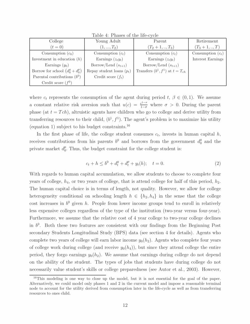
Table 4: Phases of the life-cycleCollege Young Adult Parent Retirement

(t = 0) (1, ..., T2) (T2 + 1, .., T3) (T3 + 1, .., T )

Consumption (c0) Consumption (ct) Consumption (ct) Consumption (ct)

Investment in education (h) Earnings (ztyt) Earnings (ztyt) Interest Earnings

Earnings (y0) Borrow/Lend (st+1) Borrow/Lend (st+1)

Borrow for school (dg0 + d

p0) Repay student loans (pt) Transfers (b1, f1) at t = Tch

Parental contributions (b0) Credit score (ft)

Credit score (f0)

where ct represents the consumption of the agent during period t, β ∈ (0, 1). We assume

a constant relative risk aversion such that u(c) = c1−σ

1−σwhere σ > 0. During the parent

phase (at t = Tch), altruistic agents have children who go to college and derive utility from

transferring resources to their child, (b1, f 1). The agent’s problem is to maximize his utility

(equation 1) subject to his budget constraints.16

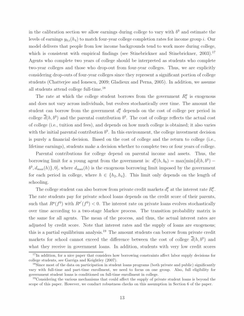
In the first phase of life, the college student consumes ct, invests in human capital h,

receives contributions from his parents b0 and borrows from the government dg0 and the

private market dp0. Thus, the budget constraint for the college student is:

ct + h ≤ b0 + dgt + dp

t + yt(h); t = 0. (2)

With regards to human capital accumulation, we allow students to choose to complete four

years of college, h4, or two years of college, that is attend college for half of this period, h2.

The human capital choice is in terms of length, not quality. However, we allow for college

heterogeneity conditional on schooling length h ∈ {h2, h4} in the sense that the college

cost increases in b0 given h. People from lower income groups tend to enroll in relatively

less expensive colleges regardless of the type of the institution (two-year versus four-year).

Furthermore, we assume that the relative cost of 4 year college to two-year college declines

in b0. Both these two features are consistent with our findings from the Beginning Post

secondary Students Longitudinal Study (BPS) data (see section 4 for details). Agents who

complete two years of college will earn labor income y0(h2). Agents who complete four years

of college work during college (and receive y0(h4)), but since they attend college the entire

period, they forgo earnings y0(h2). We assume that earnings during college do not depend

on the ability of the student. The types of jobs that students have during college do not

necessarily value student’s skills or college preparedness (see Autor et al., 2003). However,

16This modeling is one way to close up the model, but it is not essential for the goal of the paper.Alternatively, we could model only phases 1 and 2 in the current model and impose a reasonable terminalnode to account for the utility derived from consumption later in the life-cycle as well as from transferringresources to ones child.

12

in the calibration section we allow earnings during college to vary with b0 and estimate the

levels of earnings y0,i(h4) to match four-year college completion rates for income group i. Our

model delivers that people from low income backgrounds tend to work more during college,

which is consistent with empirical findings (see Stinebrickner and Stinebrickner, 2003).17

Agents who complete two years of college should be interpreted as students who complete

two-year colleges and those who drop-out from four-year colleges. Thus, we are explicitly

considering drop-outs of four-year colleges since they represent a significant portion of college

students (Chatterjee and Ionescu, 2009; Gladieux and Perna, 2005). In addition, we assume

all students attend college full-time.18

The rate at which the college student borrows from the government Rgt is exogenous

and does not vary across individuals, but evolves stochastically over time. The amount the

student can borrow from the government dgt depends on the cost of college per period in

college d(h, b0) and the parental contribution b0. The cost of college reflects the actual cost

of college (i.e., tuition and fees), and depends on how much college is obtained; it also varies

with the initial parental contribution b0. In this environment, the college investment decision

is purely a financial decision. Based on the cost of college and the return to college (i.e.,

lifetime earnings), students make a decision whether to complete two or four years of college.

Parental contributions for college depend on parental income and assets. Thus, the

borrowing limit for a young agent from the government is: dgt (h, b0) = max[min{d(h, b0) −

b0, dmax(h)}, 0], where dmax(h) is the exogenous borrowing limit imposed by the government

for each period in college, where h ∈ {h2, h4}. This limit only depends on the length of

schooling.

The college student can also borrow from private credit markets dpt at the interest rate Rp

t .

The rate students pay for private school loans depends on the credit score of their parents,

such that Rp(f 0) with Rp′(f 0) < 0. The interest rate on private loans evolves stochastically

over time according to a two-stage Markov process. The transition probability matrix is

the same for all agents. The mean of the process, and thus, the actual interest rates are

adjusted by credit score. Note that interest rates and the supply of loans are exogenous;

this is a partial equilibrium analysis.19 The amount students can borrow from private credit

markets for school cannot exceed the difference between the cost of college d(h, b0) and

what they receive in government loans. In addition, students with very low credit scores

17In addition, for a nice paper that considers how borrowing constraints affect labor supply decisions forcollege students, see Garriga and Keightley (2007).

18Since most of the data on participation in student loans programs (both private and public) significantlyvary with full-time and part-time enrollment, we need to focus on one group. Also, full eligibility forgovernment student loans is conditioned on full-time enrollment in college.

19Considering the various mechanisms that could affect the supply of private student loans is beyond thescope of this paper. However, we conduct robustness checks on this assumption in Section 6 of the paper.

13

cannot borrow at all in the private market and borrowers with low credit scores may not be

able to borrow the entire amount. Thus, the borrowing limit in private credit markets is:

dpt (h, b0, f0) ≤ min{d(h) − dg

t , dmax(f0)} with d′

max(f0) > 0. It is important to note that our

model assumes private creditors will meet the demand of student loans for borrowers with

sufficiently high credit scores.

In the next phase of life as young adults, agents consume ct, save/borrow st+1, earn labor

income ztyt(h, a) and pay back part or all of their school loans pt. They also face wage

garnishment in the case of default on government or private student loans (µg, µp). Hence,

the budget constraint is:

ct + st+1 ≤ ztyt(h, a)(1 − µg − µp) − pit; i ∈ g, p; t = 1, ..., T2; (3)

µi = 0 if pit ≥ pi

Labor income is given by the product between the deterministic component, yt(h, a) and

the stochastic component zt. The deterministic component depends on the human capital

accumulated during college such that yt(h4, a) > yt(h2, a) for any t and a. Also, for both

education groups, earnings increase in the ability level of the student a. In particular, the

premium from getting a 4 year college degree increases in a, which is consistent with the

data (details are provided in Section 4). Also earnings increase over time at a declining

rate y′t(t) > 0 and y′′

t (t) < 0.20 The idiosyncratic shocks to earnings each period, zt evolve

according to a Markov process with support Z=[z, z], where z represents a bad productivity

shock and z represents a good productivity shock. The Markov process is characterized by

the transition function Qz and it is assumed to be the same for all agents.

The agent enters repayment on both the public and the private loans. The loan amounts

at the beginning of this repayment period are given by dgt for government loans and dp

tRpt

for private loans. Note that the interest on government loans does not accumulate during

college, but it does accumulate for private loans. This is consistent with what we observe in

the data.21 We assume αit is the share of total debt the agent pays in period t toward loan i,

where i ∈ g, p and αit ∈ [0, 1]. Thus, the size of payment on student loans (both government

and private) at time t is represented by:

pt =∑

i

pit =

∑

i

αitd

it; i ∈ g, p. (4)

20We abstract from modeling human capital accumulation after college in order to focus on the role ofparental funds and credit scores in the college investment decision.

21In some cases, students pay interest on their private student loans while in college (to shorten the life ofthe loan). We abstract from this possibility.

14

Consequently debt evolves according to:

dgt+1 = dg

t (1 − αgt )R

gt and dp

t+1 = dpt (1 − αp

t )Rpt (ft); (5)

Agents default on private student loans when payments in each period are less than the

required amount, ppt < pp. In period t, the agent is required to pay the fraction αp

t which

depends on the principal of the loan ppt , the interest rate Rp

t , and the time left until the end

of the repayment phase, T2 − t. Thus, default occurs if the fraction that he chooses to repay,

αpt < αp

t . In this case, wages are garnished at the rate µp > 0. In addition, the default is

reported to credit agencies and credit scores are revised downward. Thus, when the agent

with score ft in period t chooses αpt < αp

t , the score becomes gp(αpt , ft) = f . When the

borrower pays the exact amount that it is required (αpt = αp

t ), his score does not change,

g(αpt , ft) = ft. For any payment αp

t ∈ (αpt , 1), the score is gradually updated according to

the function gp(αpt , ft) = αp

t a(ft) + b(ft), where a(ft) > 0 and b(ft) > 0. When he pays

his entire loan in period t (αpt = 1), his score improves to the next bin, gp(1, f i

t ) = f i+1t+1 for

i ∈ {1, ..., 6}.

Since we focus on the effect of credit scores on education investment via the private

market for student loans, we want to capture the feedback of the repayment behavior in this

market on the credit score. Thus, in our set-up, repayment behavior in the private student

loan market affects credit scores and the model produces a variation in credit scores across

adults later in the life-cycle. 22

Agents default on government student loans when payments are less than the required

amount, pgt < pg

t. In period t, the agent is required to pay the fraction αg

t which depends

on the principal of the loan pgt , the interest rate Rg

t , and the time left until the end of the

repayment phase, T2 − t. Thus, default occurs if the fraction that he chooses to repay,

αgt < αg

t . In this case, there are consequences to default captured by the wage garnishment

µg.23 When the agent makes the required minimum payment on government student loans

(pgt ≥ pg) , there is no wage garnishment, thus µg = 0. We require that agents must pay off

their school loans at the end of this period; thus, for t = T2, pt+1 =∑

i(dit−pi

t)Rit+1; i ∈ g, p.

As a parent, agents consume ct, borrow/lend st+1, earn labor income ztyt(h, a), and

earn/pay the risk-free rate on their last period savings/borrowings, according to:

ct + st+1 ≤ ztyt(h, a) + Rfst; t = T2 + 1, ...Tch − 1, Tch + 1, ...T3. (6)

22Our model is not a theory of credit scores. Assessing the impact of credit market participation on creditscores and explaining observed variation in credit scores across individuals is beyond the scope of this paper.

23We assume that default in the government market does not affect future credit scores.

15

Additionally, in period t = Tch, the parent transfers funds to their child b1 so that the budget

constraint is:

ct + st+1 ≤ ztyt(h, a) − b1 + Rfst − pt+1; t = Tch. (7)

Finally, the budget constraint in the last phase of life (retirement) is:

ct + st+1 ≤ Rfst; t = T3 + 1, ..., T (8)

where the agent consumes ct using his return on past period savings st.

3.2 Equilibrium

The agent i ∈ B × F × A maximizes utility (equation 1) subject to his budget constraints

(equations 2 - 8) by choosing {h, ct, st+1, αgt , α

pt , d

gt+1, d

pt+1, ft, b

1} taking prices {ztyt,Rf , Rg

t , Rpt (ft)}

and policy parameters {dmax, µg, µp} as given.

Our economy is a partial equilibrium analysis in the sense that the average interest rates

on student loans in both the government and private markets do not arise endogenously out of

an equilibrium profit condition. While this is certainly the case for the government market

in the real world, our framework may seem restrictive for the private market for student

loans. By design, the interest rate in the private market is how private creditors cover the

cost of default. Even though we do not model a general equilibrium framework, we claim

that the average interest rate in the private market captures default risk.24 We show that

our model is consistent with the fact that in a riskier environment, as measured by a higher

default rate, the average interest rate in the market charged by the private creditor is higher.

This happens for the following reasons. First, our economy features a menu of interest rates

for private loans which depend on the borrowers’ credit scores along with a feedback of the

repayment behavior on credit scores. Thus, the interest rate that the borrower faces each

period depends on the risk of default in that period, which in turn evolves over time given

the borrower’s past repayment behavior in the private market. Second, student loans are not

dischargeable after default. In our model, agents need to repay their loans in the first period

after default and they will do so at a higher interest rate since their credit scores are severely

damaged. As a result, the interest rate charged by the private creditor increases with the

average risk in the market. Nondischargeability is a key difference between the student loan

market and unsecured credit markets that allows us to take this approach.25 An important

24A standard GE setup will be intensive computationally given the high dimension of the state space andthe number of periods for the repayment phase in which the credit scores evolve.

25Chatterjee et. al. (2008) contains a theory of the terms of credit and credit scoring where the pric-

16

observation is, that in our economy, altruistic agents repay their student loans eventually.

The utility loss from transmitting a bad credit score to ones child prevents our agents from

not repaying their loans. Thus, the incentive to default declines over time. This discussion

can be conveniently explained using the present-value profit condition for the private creditor

in the economy. The functional form is given by:

PVπ =

∫

dp>0

[

T2∑

t=1

βt−1

[

∫ ∫

αpt ≥α

pt

(αpt dt)dαdRp +

∫

αpt <α

pt

∫

(µpztyt)dzdα

]

− dp0

]

df

Note that the private creditor collects a wage garnishment from defaulters during the

period when default occurs and collects repayments every period until the loan is paid in

full from all participants in the private market, including defaulters (except for the period

when default occurs). These payments, αpt (dt, R

pt (ft), T2 − t), depend on the time left for

repayment, the principal and the per period interest rate, which in turn depends on the credit

score of the borrower. The credit score is updated each period given the repayment behavior

in the previous period, ft+1 = g(αpt , ft). We assume that the private creditor borrows in the

risk-free capital market and so the difference between the present value of repayment and

the loan amount is positive and increases in the case where default is more likely to occur. In

the results section, we calculate total profit for the private creditor in the policy experiments

and compare them to the benchmark economy, and show that the average profit is increasing

in the default risk. This monotonicity is mostly due to the difference between repayment

and the loan amount, rather than the wage garnishment. Thus, the average interest rate

captures most of the default risk whereas the wage garnishment captures only a small part

of it.

We recast the problem in a dynamic programming framework and solve backwardly for

of all the choices in the model. The value functions for the four phases in the life-cycle are

given below. For the retirement phase, the value function is:

V4(s, t) = maxs′

u(s(1 + r) − s′) + βV4(s′, t + 1).

ing of default risk is generated out of the zero-profit condition in a general equilibrium framework withdischargeability rules.

17

For the parent phase, there are three value functions:26

Vpost3 (a, h, s, z, t) = max

s′

u(zy(h, a) + s(1 + r) − s′) + βEz′ V

post3 (a, h, s′, z′, t + 1);

Vpar3 (a, h, s, f1, z, T ch) = max

s′,b′u(zy(h, a) + s(1 + r) − s′ − b1) + βEz

′ Vpost3 (a, h, s′, z′, T ch + 1) + βρV ch

3 (b1, f1)

Vpre3 (a, h, s, f1, z, t) = max

s′

u(zy(h, a) + s(1 + r) − s′) + βEz′ V

pre3 (a, h, s′, f1, z′, t + 1).

with V ch3 (b1, f 1) = (1−φ)b1(1−σ)/(1−σ)+φd(f)1(1−σ)/(1−σ). We assume separability in b1

and f 1 such that x(b1, f 1) = (1−φ)ω(b1)+φν(f 1) and ν ′, ω′ > 0, ν ′′, ω′′ < 0. The parameter

φ measures the relative weighting that parents put on transferring funds to their child versus

transferring their credit score.

For the young adult, the value function is given by:

V2(a, h, s, f, dp, dg, rp, rg, z, t) = maxαp,αg,s′

u(zy(h, a) + s(1 + r) − s′ − αidi) +

βEr′

i,z

′V 2(a, h, s′, f ′(αp), d′

p(αp), d′

g(αg), r′

p,r′

g, z′

, t + 1),

with i ∈ {g, p}. Finally, for the college phase, the value function is given by:

V1(a, b, f, rp, rg, 1) = maxh

u(b − h + dp(b, f, h) + dg(b, h) + y(h) + βjEr′

i,z

′V2(a, h, f ′(αp), d′

p, d′

g, r′

p,r′

g, z′

, 2)

where j ∈ {1, 2} in case h ∈ {h2, h4}.

4 Parameterization

The model period and phases are detailed in Table 5. Each model period represents one

year, and agents live for 55 years (T = 55). The first phase (college) lasts 4 years, the young

adult phase lasts 10 years, the parent phase lasts 24 years, and the retirement phase lasts

20 years. Thus, T1 = 1, T2 = 11, T3 = 35, T = 55. The period when parental transfers

are made to their child is Tch = 22 and is set to match the average parental age of college

students (which is 43 years old).

There are four sets of parameters that we calibrate: 1) standard parameters such as the

discount factor, the coefficient of risk aversion, the coefficient of altruism, the risk free interest

rate; 2) parameters for the initial distribution of characteristics: parental income, credit

scores and student’s ability; 3) parameters specific to student loan markets such as college

costs, tuition, borrowing limits, default consequences, interest rates on student loans, etc.;

26In the computations, we divide the problem for the parent phase into three sub-phases: post-child, child,and pre-child. Also, we introduce an extra feature for the young adult phase: a finer grid for the credit scores(other than the 6 bins mentioned above), which are needed for the evolution of credit scores over time.

18

Table 5: Model periods and phasesPhase Age Years Periods (t)College 18-22 4 1

Young Adult 23-32 10 2-11Parent 33-56 24 12-35

Retirement 57-76 20 36-55

and 4) parameters for the earnings dynamics of individuals by education and ability groups.

Our approach includes a combination of setting some parameters to values that are standard

in the literature, calibrating some parameters directly to data, and jointly estimating the

parameters that we do not observe in the data by matching moments for several observable

implications of the model. More specifically, we jointly estimate seven parameters: the wage

garnishment for government and private loans, the mean and standard deviation from the

initial distribution of parental contributions, and earnings during college by income treciles.

These seven parameters are set to match seven targets: the national two-year cohort default

rates in both the government and private student loan market (5.5% and 4.0%), the four-

year college completion rate by income treciles from BPS data (57%, 64.6% and 82.7%), and

the participation rates in the government and private student loan market from the College

Board (50%, 30%). Table 6 reports how well the model does in replicating the seven data

points. We provide details on the procedure in the following subsections.

Table 6: Model Predictions vs. DataParameter Name Value Variables Targeted Data Model

Earnings during college for: 4-year college completion rate:

yT1,1(h4) 1st trecile of income $18,009 1st trecile of income 57% 50.1%

yT1,2(h4) 2nd trecile of income $6,552 2nd trecile of income 64.6% 65.4%

yT1,3(h4) 3rd trecile of income $4,968 3rd trecile of income 82.7% 81%

µb Mean of parental contribution $41,245 Participation rate in govt mk 50% 51%

σb St. dev. of parental contribution $38,839 Participation rate in private mk 30% 29%

µg Wage garnishment govt mk 0.035 Default rate in govt mk 5.4% 5.4%

µp Wage garnishment private mk 0.05 Default rate in private mk 3.9% 3.9%

Figures are in 2007 dollars.

Table 7 reports the values for the remaining parameters of the model. The discount

factor is set to match the risk free rate (Rf) of 4%, thus β =0.96. We assume a CRRA

utility function with the coefficient of risk aversion as standard in the literature, σ = 2.

In setting the parameter for altruism, ρ, we use estimates from Nishiyama (2002). His

calibrated altruism parameter is 0.626 for a coefficient of relative risk aversion of 2. We

set the parameter φ, which measures the relative weighting that parents put on transferring

19

Table 7: Parameter ValuesParameter Name Value Target/Source

β Discount factor 0.96 Real avg rate=4%σ Risk aversion coeff 2 Literatureρ Coef of altruism 0.626 Nishiyama (2002)φ Weighting of credit scores 0.5 —

Tchild Period of parental contribution 22 Avg age of college students’ parentsRf Risk-free rate 1.04 Average rate in 2000-2008

funds to their child versus transferring their credit score to φ = 0.5. We run robustness

checks on this parameter and know that is does not alter our main findings. We assume

CRRA functions with σ = 2. We evaluate the utility one derives from consuming b1 and

from consuming the level of debt that one can obtain in the private market for a given f 1

evaluated at the interest rate Rpi . We assume a uniform grid for debt, that ranges from 0

to the maximum amount of debt that can be obtained in the private market for the average

level of parental contributions. We run robustness checks and find that our results are not

sensitive to these debt levels as long as credit scores induce heterogeneity in the amounts

that one can borrow.

In what follows, we discuss in detail the parameterization of the initial distribution of

individual characteristics, the parameters specific to the student loan market, and earnings

dynamics.

4.1 Initial Distribution of Parental Contributions, Credit Scores

and Ability

For the parental contribution for college, we consider a uniform grid, B = [0, 100, 000] in

2007 dollars with 20 levels of b0. For initial credit scores, we set six bins corresponding to

the bins used by Sallie Mae to determine the conditions on student loans, F = {< 640, 640−

669, 670− 699, 700− 729, 730− 759, 760− 850}. We measure the ability level, a, by the SAT

scores of students and consider 3 groups of SAT scores: A = {< 900, 900−1100, 1100−1600}

corresponding to treciles of SAT scores.

We estimate a joint distribution of parental contribution, credit scores, and ability ac-

counting for correlations between all these three characteristics. We assume a normal dis-

tribution for parental contributions for college, B(b0) ∼ (µb, σb). While the expected family

contribution is a good predictor for the actual parental contribution for college, differences

may arise between the two. Rather than using an exogenous distribution for the expected

family contribution for college, we estimate the moments of the distribution of parental

20

contributions to match participation rates in the government student loan and the private

student loan market (50% and 30%). Recall that the parental contribution determines the

mass of people who are eligible to borrow under the government market and also those for

whom the borrowing limit binds. We assume that all borrowers who face this borrowing

limit in the government market will turn to the private market. We obtain µb = $41, 245

and σb = $38, 839 in 2007 constant dollars, which are consistent with the Baccalaureate and

Beyond (B&B) data from the U.S. Department of Education that yields a mean expected

parental contribution of $52,250 (over four years of college) and a standard deviation of

$37,943.27

For the distribution of credit scores, F (f 0), we use the national distribution of FICO

scores provided in Section 2.3 and assume a normal distribution where F ∼ (716, 54). For

the distribution of ability, A(a), we use the national distribution of SAT scores and assume

a normal distribution with a mean of 1016 and a standard deviation of 226 (College Board,

2007).

Our model assumes a positive correlation between all three initial characteristics.28 Based

on the results in section 2.2, there is a small, positive correlation between credit scores

and parental contribution for college, such that ρ(b0, f0) = 0.15, where ρ is the correlation

coefficient. For the correlation between ability and initial parental contributions, we use

ρ(b0, a0) = 0.4, which is in the middle of the estimates from Ionescu (2009).

4.2 Student Loan Parameters

4.2.1 College Costs and Loan Limits

Recall that the amount agents can borrow from the government is represented by: dg0 =

max[min{d(h, b0) − b0, dmax(h)}, 0], where d(h, b0) is the net price of college, b0 represents

parental contributions to college, and dmax(h) is the exogenous borrowing limit imposed by

the government.

To set the appropriate borrowing limits for government school loans, we need the net

price of college, which is total student charges (tuition, fees, room and board) net of grants

and education credits, as reported by the College Board (2007a). We calibrate the model to

academic years 2003-2004 through 2007-2008. The net price of college for these four years

was $88,380 for private universities and $38,080 for public universities (in 2007 dollars). The

net price for a two-year college was $13,920 (for two years). Since agents in the model pay

27http://nces.ed.gov/surveys/hsb/index.asp28Our findings from the SCF data presented in Section 2 show a positive correlation between credit scores

and income. In addition, data suggest a strong positive correlation between SAT scores and parental income(see College Board, 2009).

21

for college as a consumption good (h), we must also calculate the total direct cost of college

in terms of tuition and fees. Total tuition and fees for four-year private and public colleges

and two-year public colleges were $90,657, $23,541, and $4,671 (for two years), respectively,

using the same College Board data.

To match the actual costs of attending four years and two years of college, we use the BPS

data on dropout and completion rates for the cohort of students starting college in 1995-96.

Our sample consists in high-school graduates who enroll in four-year and two-year colleges,

are enrolled exclusively full-time and without a delay after graduating from high-school. Also,

we consider students with SAT scores above 700. According to the national distribution of

SAT scores, less than 8 percent of students have scores below 700. Also according to the BPS

data, 56% of these students enrolled in less than two-year colleges or enrolled into two-year

colleges and dropped out, 45% delayed their enrollment in college and 55% did not enroll

full-time in the first semester when they enrolled in college and thus were not eligible for

student loans. The four-year college group consists of college graduates, i.e. students who

obtained their bachelor degree by 2001. Those who drop-out of four-year colleges are put

into the two-year college group. The 2-year college group also includes those who complete a

two-year degree (those who drop-out of two-year colleges are not considered). We find that

67% of students completed a four-year degree (59.1% of these students attended a public

institution and 40.9% a private institution) and 33% completed a two-year degree (71.2%

of these students were drop-outs from four-year colleges and 28.8% completed a two-year

degree).29 Using these weights and assuming they have been constant over time, the average

net price for getting a four-year degree is $58,654. For two years of college, the net price is

$20,535.30 The average direct costs (tuition and fees) using the same weights are: $50,993

for a four-year degree and $18,762 for two years of college.

Our setup focuses on the duration of college investment while ignoring college hetero-

geneity in other dimensions such as quality of the school. However, we recognize the fact

that students from different family background may sort into different types of schools and

we allow the cost of college to vary with student income. In particular, our findings from

the 1996 BPS sample show that the cost of college increases in the income level of students.

An interesting finding is that the relative cost of four years of college relative to two years

of college declines in the parental income of students. This is an essential feature to be

captured in our model so that we can correctly account for the borrowing behavior in the

two markets for student loans and the relevance of credit scores for borrowing and college

29http://nces.ed.gov/programs/coe/2004/section3/table.asp?tableID=6130Note that for drop-outs of 4-year colleges, we assume they pay the net price of attending a 4-year college

(public and private) for 2 years. Thus, our 2-year net cost is higher than the cost of 2-year colleges since itincludes drop-outs from 4-year colleges that paid a much higher net price.

22

investment behavior. We measure students’ income by the expected family contribution and

look at college costs by income treciles. Since the BPS data provide information only for the

cost of college in the first academic year, we use these measures and obtain relative differ-

ences in the cost of college for two and four years of college across income treciles. We apply

these differences to the average cost of college for four and two years of college and obtain

college costs by institutions and income groups of students as follows: for the four-year group

the costs are $57,716, $56,777, and $60,942 and for the two-year group, costs are: $19,180,

$20,535, and $24,231.31

With respect to government student loans, the Stafford loan limit for dependent under-

graduates is $23,000 for up to five years of post-secondary education. Dependent students

who enroll in college for two years are eligible for $6,125 in Stafford loans during this period

($2,625 for the first year and $3,500 for the second year of college). As a percent of average

net college price, students attending four-year institutions could therefore borrow approxi-

mately 40% of the net average college price from the federal government. Students attending

college for two years could borrow 30% of the net average college price from the government.

Note that unlike the cost of college, these limits do not vary with the income of students. As

a result, the limits represent a higher percentage of net college cost for low-income students

than for high-income students.

Loan limits in the private market for school loans are set by the creditor and do not

exceed the cost of college less any financial aid the student receives, including government

student loans in the case of borrowers with a good credit score. In addition to this, borrowers

with credit scores lower than 640 cannot borrow in the private market and borrowers with

credit scores lower than 700 cannot borrow more than the average amount that it is borrowed

in the private market. Thus, the borrowing limit in private credit markets is: dpt (h, b0, f0) ≤

min{d(h, b0) − dgt , dmax(f0)} with dmax(f0) = 0 if f0 < 640, dmax(f0) = mean(dp) if 640 ≤

f0 < 700 and dmax(f0) = d(h, b0) if 700 ≤ f0.

4.2.2 Student Loan Interest Rates and Default Penalties

The interest rates on government and private student loans follow a stochastic process,

given by a 2 by 2 transition matrix Π(Rg′, Rg) on {Rg, Rg} and Π(Rp′ , Rp) on {Rp, Rp}.

The interest rates on private loans depend on credit scores, whereas the interest rate on

government loans do not.

The government sets the interest rates based on the 91-day Treasury-bill rates plus a

margin of 3.1%. We use the time series for 91-day Treasury-bill rates for 2000-2007, adjusted

31Certainly our calculations are simplified in assuming that the weight for private and public schools arethe same across income groups of students.

23

for inflation. We fit the time series with an AR(1) process: Rt = µ(1 − ρ) + ρRt−1 + ε,

ε ∼ N(0, σ2), which yield estimates of ρ = 0.9902 and σ = 0.2097 and mean 3.11%. We

aggregate this to annual data; the autocorrelation is given by 0.89 and the unconditional

standard deviation by 1.511. We approximate this process as a two-state Markov chain. The

support is Rg ∈ {1.047, 1.0772}, and the transition matrix is

[

0.7037 0.2963

0.2963 0.7037

]

.

Sallie Mae sets the interest rates based on the 3-month LIBOR rates plus a margin

that differs across credit scores, which are described in Table 4.32 We consider 6 bins of

credit scores on the set F = [f, f ] corresponding to the 5 groups of FICO scores in Table

4, including the group with FICO scores less than 640.33 The minimum FICO score that

Sallie Mae would accept for private student loans was 640 in 2008; thus, for any credit

scores below 640, dp = 0. We use the time series for 3-month LIBOR rates between 2002-

2007 and fit it with an AR(1) process. The estimates of the two moments are given by

ρ = 0.9888 and σ = 0.2117 and the mean is 3.41%. We aggregate this to annual data; the

autocorrelation is given by 0.872 and the unconditional standard deviation by 1.408. We

have approximated this process as a two-state Markov chain. The support for each of the

bins of credit scores is Rp1 ∈ {1.06, 1.0882}, Rp

2 ∈ {1.085, 1.1132}, Rp3 ∈ {1.105, 1.1332}, Rp

4 ∈

{1.125, 1.1532}, and Rp5 ∈ {1.14, 1.1682}. The transition matrix is

[

0.7003 0.2997

0.2997 0.7003

]

.

We calibrate the default punishments to match the repayment behavior in the data. We

set the wage garnishment for default in the government student loan market as µg = 0.035

to match the default rate for government student loans of 5.4% in 2007. In practice this

punishment varies across agents, depending on collection and attorney’s fees, and can be as

high as 15%. The wage garnishment for private student loans µp = 0.05 is set to match

the default rate for private student loans, which is 3.92%. Also, recall that the repayment

behavior in the private market affects the credit score of the individual. The fraction of the

student loan that is paid in period t is αpt for private loans. When the agent chooses αp

t

such that ppt = αp

t dpt < pp = αp

t dpt , the score is severely damaged and becomes f . For any

payment greater or equal than the minimum require in each market, the score is gradually

updated according to the function gp(αpt ,ft)=αp

t a(ft)+b(ft). When the borrower pays the

exact amount that it is required in each of these markets, his score does not change, f i

and when he pays his entire loan in period t, his score improves to the next bin, f i+1 for

i ∈ {1, ..., 6}. We use these upper and lower bounds for each bin of credit scores in each

market and compute the linear function for the credit score evolution on a finer grid of credit

32The margins are from June 2008 and were obtained from: http://www.salliemae.com/about/investors/33We compute the interest rate on private college loans based on the mean of 3-month LIBOR rate for the

period December 2000-December 2007.

24

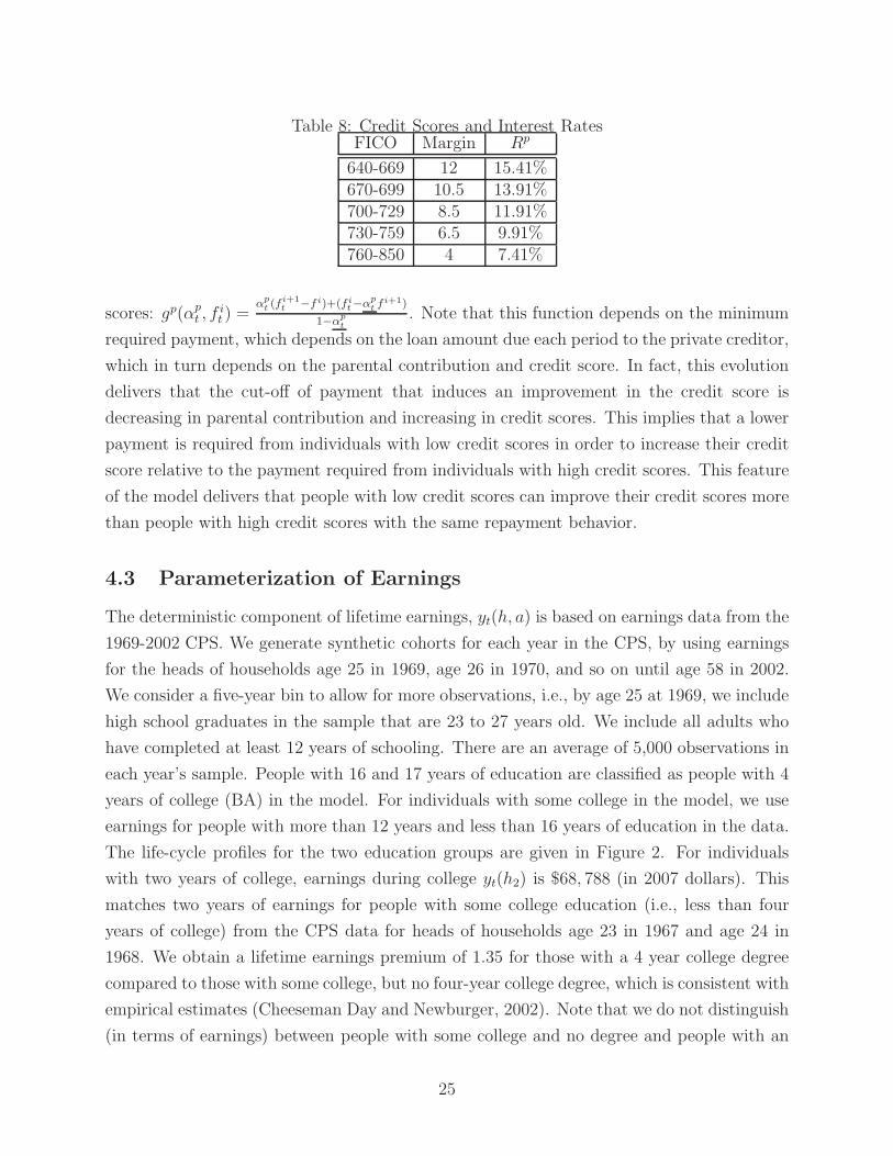
Table 8: Credit Scores and Interest RatesFICO Margin Rp

640-669 12 15.41%670-699 10.5 13.91%700-729 8.5 11.91%730-759 6.5 9.91%760-850 4 7.41%

scores: gp(αpt , f

it ) =

αpt (f i+1

t −f i)+(f it−α

pt f i+1)

1−αpt

. Note that this function depends on the minimum

required payment, which depends on the loan amount due each period to the private creditor,

which in turn depends on the parental contribution and credit score. In fact, this evolution

delivers that the cut-off of payment that induces an improvement in the credit score is

decreasing in parental contribution and increasing in credit scores. This implies that a lower

payment is required from individuals with low credit scores in order to increase their credit

score relative to the payment required from individuals with high credit scores. This feature

of the model delivers that people with low credit scores can improve their credit scores more

than people with high credit scores with the same repayment behavior.

4.3 Parameterization of Earnings

The deterministic component of lifetime earnings, yt(h, a) is based on earnings data from the

1969-2002 CPS. We generate synthetic cohorts for each year in the CPS, by using earnings

for the heads of households age 25 in 1969, age 26 in 1970, and so on until age 58 in 2002.

We consider a five-year bin to allow for more observations, i.e., by age 25 at 1969, we include

high school graduates in the sample that are 23 to 27 years old. We include all adults who

have completed at least 12 years of schooling. There are an average of 5,000 observations in

each year’s sample. People with 16 and 17 years of education are classified as people with 4

years of college (BA) in the model. For individuals with some college in the model, we use

earnings for people with more than 12 years and less than 16 years of education in the data.

The life-cycle profiles for the two education groups are given in Figure 2. For individuals

with two years of college, earnings during college yt(h2) is $68, 788 (in 2007 dollars). This

matches two years of earnings for people with some college education (i.e., less than four

years of college) from the CPS data for heads of households age 23 in 1967 and age 24 in

1968. We obtain a lifetime earnings premium of 1.35 for those with a 4 year college degree

compared to those with some college, but no four-year college degree, which is consistent with

empirical estimates (Cheeseman Day and Newburger, 2002). Note that we do not distinguish

(in terms of earnings) between people with some college and no degree and people with an

25

associate degree. More generally, in our model what matters for earnings differences by

education groups is the duration of college education rather than the acquired degree. Kane

and Rouse (1993) find that degree recipients do not earn more than non-degree recipients

with the same number of credits. Bound, Lovenheim and Turner (2009) document that

the average number of years of college for people a bachelor’s degree is 5.3 years. Thus, the

college degree premium that we use delivers an average return per additional year of college

education of roughly 10%, which is consistent with estimates in the literature (Willis, 1986;

Restuccia and Urrutia, 2004).

Earnings also vary with the ability level of the individual, as measured by SAT scores. We

use annual earnings by education groups in the fifth year after acquiring the highest degree

for college-going high school graduates in the National Education Longitudinal Study of 1988

(NELS:88) data set. Similar to our analysis based on the BPS data, we construct a sample of

high-school graduates that enrolled in college full-time without a delay (the cohort of 1992).

We group individuals by treciles of SAT scores, i.e. ≤ 900, 900− 1100, and > 1100. We find

that earnings increase in the SAT score regardless of the education level of the individual

(2 years versus 4 years). Furthermore, the premium from completing 4 year college relative

to 2 year increases in the ability level, but at a declining rate. We apply these earnings

differences between students with four years and two years of college by SAT scores to the

annual earnings from the CPS data for the two education groups. We obtain the following

differences in premia from acquiring a college degree over the lifecycle: 1.272, 1.338 and 1.341

across the three ability groups. Our calibration is consistent with empirical evidence that

individuals of higher ability levels experience higher returns to their education investment

(see Rosen and Willis (1979), Cuhna et al. (2005), Heckman and Vytlacil, 2001). Also,

most of the increase in returns is captured by the difference between the first and the second

trecile of ability, which is consistent with the findings in Ashenfelter and Rouse (1998) and

Hendricks and Schoellman (2009). An important observation is whether these returns are

due to the innate ability of the individual or the quality of the school these individuals attend

before college or the quality of college itself or it is primarily due to family characteristics.

In our case, we directly consider a measure of ability that embodies both innate ability

and acquired ability since we think of the ability as college preparedness. In addition, our

model captures a correlation between ability and parental income. Finally, empirical findings

show that returns to schooling are mostly driven by the ability of the student and length of

schooling rather than the quality of the school.34

Finally, students can work during college in the model. We pick the value of earnings dur-

34Dale and Krueger (1999) find that students who attend more selective colleges do not earn more thanother students who were accepted and rejected by comparable schools but attended less selective colleges.

26

Figure 2: Lifetime Earnings - CPS data

25 30 35 40 45 50 55

3

4

5

6

7

8

9

10x 10

4 Earnings By Education Groups

Age

2 year college4 year college

ing college across income treciles in the model to match the fraction of college students that

complete 4 years of education across individuals from treciles of expected family contribution

in the BPS sample: 57% , 64.6% and 82.7%. We obtain $18,009, $6,552, and $4,968 for

earnings during college. Our calibration produces declining earnings by parental income of

students. Even though we do not model time allocation between market and school work

during college, our model captures the fact that some students may use earnings during

college to supplement funds needed to invest in college (which is consistent with findings

in Garriga and Keitly(2007). Also, according to the NCES data, 46% of full-time enrolled

college students choose to work during college years (Berkner, He, and Cataldi,2002). Fur-

thermore the model captures the fact that people from low income backgrounds work more

during college and thus may decrease their chances of acquiring a college degree. Divert-

ing time from school work to job work may affect school performance. Research finds that

working during college has a significant impact on dropping out (see Manski (1983) and

Stinebrickner and Stinebrickner (2003) for details).

In the parameterization of the stochastic idiosyncratic labor productivity process, we

follow Storesletten, Yaron and Telmer (2001) who build a panel from the Panel Study of

Income Dynamics (PSID) to estimate the idiosyncratic component of labor earnings. They

use annual data from PSID from 1968 to 1991 for wage earnings. With uij = ln(zij), the

stochastic part of the labor income process for household i at time j, the estimated model

27

is:

uij = yij + ǫij

yij = ρyi,j−1 + νij

where ǫij N(0, σ2ǫ ) and νij N(0, σ2

ν) are innovation processes. The variables yij and ǫij are

realized at each period over the life cycle and are referred to as persistent and transitory

“life-cycle shocks”, respectively. Fernandez-Villaverde and Krueger (2002) report ρ = 0.935,

σ2ǫ = 0.017, and σ2

ν = 0.061. We have approximated this process as a two-state Markov

Chain, normalizing the average value for the idiosyncratic shock to be 1. The resulting

support is the set Z = {0.8266, 1.1734} with the transition probability matrix given by[

0.89 0.11

0.11 0.89

]

.

5 Quantitative Results

5.1 Benchmark

In the benchmark economy, the four-year college completion rate is 65.6 percent. This

represents the percentage of students who complete four years of college, out of the pool

of all college students (i.e., those who complete two and four years of college). Students in

the model borrow on average $31,050 (in 2007 dollars) to finance college: $15,028 from the

government and $16,022 from the private market. Not surprisingly, since the cost of financing

four years of college is significantly higher than financing two years of college, students with

four years of college borrow $39,682 (from both sources) compared to $12,458 for students

with four years of college, as evident in Table 9. However, in both cases, more than half

of borrowed funds is from the private student loan market. Thus, the private student loan

market is an important source of funds for college students in the model.

Default rates in the government and private student loan markets are 5.4 and 3.9 percent,

respectively. For the benchmark economy, all of the default comes from students with four

years of college.35 Students with four years of college take on three times as much debt as

students with two years of college. Higher debt levels necessary to finance the additional

years of college may be accompanied with large adverse earnings shocks, which pushes agents

with four years of college into default. Conversely, the relatively low cost of acquiring two

35This is due to the fact that students with two years of college in the model do not include those withmore than two years of college who do not complete the bachelor’s degree. These students have large amountof student debt, relatively low income (since they did not complete the degree), and high default rates, butare not captured in our model, such that default rates for the two-year college group are understated.

28

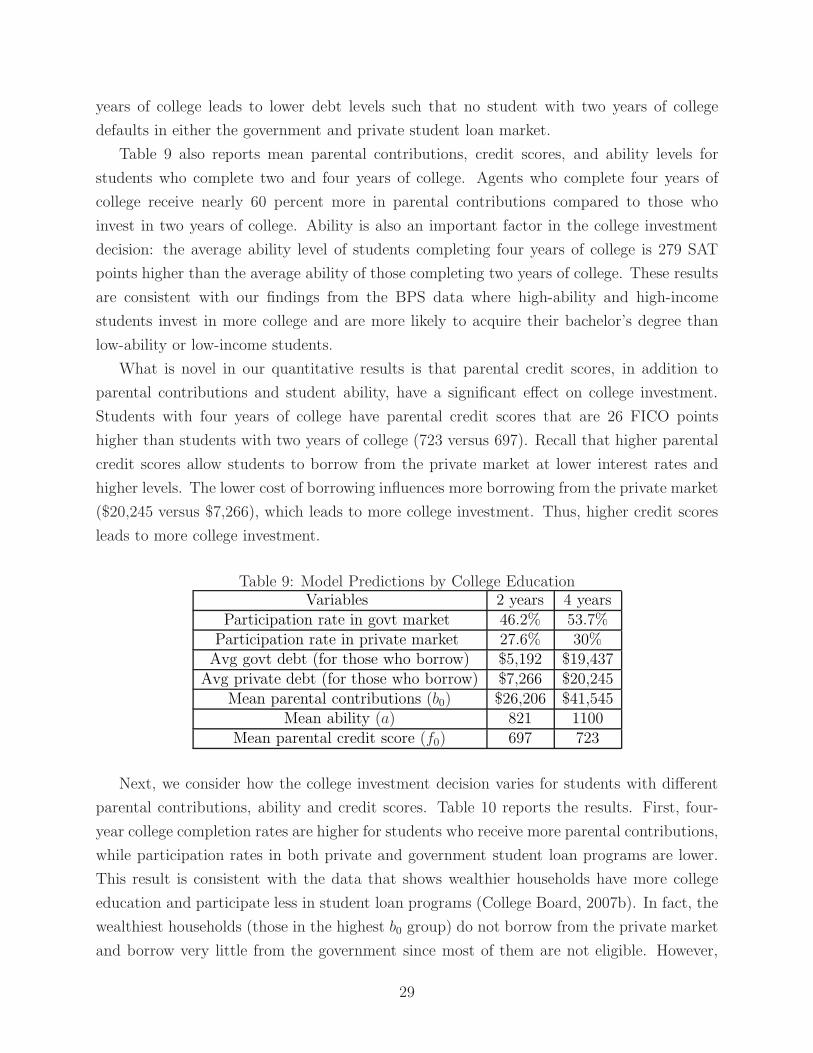
years of college leads to lower debt levels such that no student with two years of college

defaults in either the government and private student loan market.

Table 9 also reports mean parental contributions, credit scores, and ability levels for

students who complete two and four years of college. Agents who complete four years of

college receive nearly 60 percent more in parental contributions compared to those who

invest in two years of college. Ability is also an important factor in the college investment

decision: the average ability level of students completing four years of college is 279 SAT

points higher than the average ability of those completing two years of college. These results

are consistent with our findings from the BPS data where high-ability and high-income

students invest in more college and are more likely to acquire their bachelor’s degree than

low-ability or low-income students.

What is novel in our quantitative results is that parental credit scores, in addition to

parental contributions and student ability, have a significant effect on college investment.

Students with four years of college have parental credit scores that are 26 FICO points

higher than students with two years of college (723 versus 697). Recall that higher parental

credit scores allow students to borrow from the private market at lower interest rates and

higher levels. The lower cost of borrowing influences more borrowing from the private market

($20,245 versus $7,266), which leads to more college investment. Thus, higher credit scores

leads to more college investment.

Table 9: Model Predictions by College EducationVariables 2 years 4 years

Participation rate in govt market 46.2% 53.7%Participation rate in private market 27.6% 30%

Avg govt debt (for those who borrow) $5,192 $19,437Avg private debt (for those who borrow) $7,266 $20,245

Mean parental contributions (b0) $26,206 $41,545Mean ability (a) 821 1100

Mean parental credit score (f0) 697 723

Next, we consider how the college investment decision varies for students with different

parental contributions, ability and credit scores. Table 10 reports the results. First, four-

year college completion rates are higher for students who receive more parental contributions,

while participation rates in both private and government student loan programs are lower.

This result is consistent with the data that shows wealthier households have more college

education and participate less in student loan programs (College Board, 2007b). In fact, the

wealthiest households (those in the highest b0 group) do not borrow from the private market

and borrow very little from the government since most of them are not eligible. However,

29

Table 10: Variation in Initial Characteristics: Benchmark4-year college Participation rates Average debt Default rates

completion rate (govt/private) (govt/private) (govt/private)

Parental Contributions (b0) for those who borrow

Low 50.1% 97.8%/77.4% $14,780/$17,326 7.8/4.4

Medium 65.4% 55.5%/9.6% $15,400/$5,216 1.3/0

High 81% 5.4%/0% $2,664/0 0/-

Ability of the student (a)

Low 27.6% 47%/38% $15,462/$18,816 13.2/4.5

Medium 79.8% 66%/33% $14,780/$13,538 2.3/2.4

High 89.1% 40%/16% $14,966/$14,345 1.5/5.7

Parental credit score (f0)

Low 51% 56.7%/23.7% $10,557/$7,204 3.8/0

Medium 67.2% 51.3%/33.6% $15,525/$14,221 5.1/5.4

High 78.3% 45.3%/29.7% $19,996/$24,026 8/5.5

Note: For parental contributions, the low group ranges from $0-$25,337, the medium group from $25,338-$58,622, and the

high group over $58,622. For ability, the low group ranges consists of ability index less than an SAT score of 900, the medium

group from 900-1,100 SAT scores, and the high group greater than an SAT of 1,100. For credit scores, the low group ranges

from 640-689, the medium group from 690-735, and the high group from 736-850.

middle-income students heavily rely on the government student loan market, as evidenced

by their 56 percent participation rate and $15,400 average government loan.

Approximately one-half of the poorest students in the model (those in the lowest b0

group) complete four years of college. There are several factors at play here. First, since

ability and parental contributions are positively correlated in our framework, the poorest

students in the model experience relatively low returns to college investment. In addition,

the relative cost of four years of college (compared to two years of college) is highest for poor

students, as documented in the calibration. The combination of relatively low returns to

college investment and the high cost of college explains the relatively low four-year college

completion rate for this group of students. However, poor students are assumed to earn

the most in the form of supplemental income during college (which is consistent with the

data). The extra earnings allow some of them to invest in college, despite their low parental

contributions.

Notice (in Table 10) that students with the lowest parental contributions take on the

most student loan debt (more than $32,000 for the average borrower), even though only half

complete four years of college. They are eligible for more student loans (both government

and private) since their parental contributions are low. Thus, poor households are borrowing

at relatively high levels just to complete two years of college. Large amounts of student loan

debt and low lifetime earnings lead to high default rates for this group. In fact, the poorest

30

students have the highest default rates, making them the most risky borrowers in the model.

Not surprisingly, high-ability students (those in the top third of ability levels) have the

highest four-year college completion rates, at 89 percent. This compares to low ability

students, with a four-year college completion rate of only 28 percent. In addition, Table 10

illustrates a large increase in four-year college completion rates between low- and medium-

ability agents, from 28 percent to 80 percent. This is due to a large increase in relative

earnings between these two types of agents, as documented in the calibration.

Participation in the private student loan market falls in ability, such that students with

the lowest abilities borrow from the private market the most. This is not true for the govern-

ment student loan market: agents with medium level of ability borrow from the government

at higher rates than those with low and high ability, which is consistent with the data.36 High

participation in the government student loan market by agents with medium level of ability

and their consequent high four-year college completion rates suggest that the government

student loan program is effective in promoting college investment for this group of students.

To our knowledge, we are the first to report differences in borrowing behavior across ability

types that are consistent with the data. Most other models of student borrowing (Lochner

and Monge-Naranjo, 2008; Ionescu, 2009) infer that participation in the government student

loan program would rise in ability, which contrasts to our findings in the model and in the

data.

Table 10 confirms the positive relationship between credit scores and college investment.

Agents with the lowest parental credit scores borrow from private markets less often and

invest less in college than agents with higher parental credit scores. This is attributed to the

fact that students with the lowest parental credit scores receive the worst loan conditions and

hence are less likely to borrow from private creditors. What is surprising is that participation

in the private student loan market is slightly lower for agents with the highest parental

credit score (above 735), compared to agents with parental credit scores in the middle range

(between 690 and 735). For those who borrow from private markets, the amount they borrow

is higher, which is consistent with having access to cheaper loans. But fewer of them borrow

(from both the private and government market). Agents with the highest parental credit

scores have the most to lose from defaulting in the private market: if they default, their credit

scores will be severely revised downward. Thus, students with high parental credit scores

prefer to default in the government student program. However, there is some incentive for

students with high credit scores to default in the private market given their relatively high

debt burden. This counteracts the repayment incentives created by the penalty on credit

36The 2003 cohort of the BPS shows that borrowing rates and levels were highest for students in the middlethird of the ability distribution, as measured by SAT scores.

31

scores as a result of default. Therefore, students with high credit scores default at high rates.

In this environment where interest rates in the private market for student loans depend

on credit scores, there is an important role for earnings uncertainty. For students who borrow

from the private market, interest rates can be twice as high for someone in the lowest range of

credit scores compared to someone in the highest range of scores. Thus, the cost of a student

loan, especially when financed over ten or more years, can be significantly higher for students

with low credit scores. If this student experiences a bad shock in lifetime earnings, this may

significantly reduce college investment. Thus, earnings uncertainty in this model amplifies

the effects that credit scores have on college investment, compared to an environment without

earnings uncertainty.

Notice that, in general, students are using the private market for student loans in con-

junction with the government student loan program. Students with better parental scores

borrow more (in levels) from both the private and government market compared to students

with low parental scores. Similarly, poor students use both student loan markets more than

rich students. Thus, it seems as if the two program are complementary: students are using

a mix of parental contributions and private and public loans to finance college, which is

consistent with the results of Lochner and Monge-Naranjo (2008).

Since parental contributions and ability are important determinants of college investment,

our results imply that poor students can achieve relatively high four-year college completion

rates, as long as their parent’s credit score is high enough. In addition, we document that

good parental credit scores have significant effects on the college investment decision for

students with medium levels of abilities. Thus, the private market for student loans pro-

vides students with another mechanism to fund college through the use of credit scores, and

that this market may be especially important for low-income and medium-ability students.

However, credit scores are not as important in the college investment decision for wealthy

students since their high levels of parental contributions and ability lead to high four-year

college completion rates independent of participation in the private market.

To recap, the benchmark economy delivers several interesting findings. We find that

parental credit scores have quantitatively significant effects on the college investment deci-

sion. Students with the highest credit scores, who get attractive interest rates on private

loans, borrow at very high levels from both the private market and the government to finance

college. This leads to high college completion rates for this group. However, for those with

low credit scores, it is very costly to borrow from the private market. As a result, they invest

less in college, and have four-year college completion rates that are 27 percentage points

lower than students with high credit scores.

Poor students in the model borrow at high levels from both the government and private

32

market; however, they complete four years of college at much lower rates, leading to low

lifetime income, and high default rates. In fact, default rates in both the government program

and private markets are highest for students from the poorest families, making them the

most risky creditors. However, poor students with relatively good credit scores benefit from

having access to the private market for student loans to the extent that their four-year college

completion rates increase with their credit score. Thus, the existence of a private market for

student loans is important for low-income students.

We also find that ability matters for college investment, and in a way that is intuitive (the

highest ability agents invest the most in college). However, the method of financing college

varies across ability levels. Participation rates in the government program are highest for

medium-ability students, while participation in the private market is highest among low-

ability students.

5.2 Policy Experiments

We next conduct two policy experiments. First, we consider the case in which the government

increases the maximum borrowing limit on government student loans. Second, we tighten

the conditions for obtaining student loans from the private market. Table 11 summarizes

the results for the experiments.

Table 11: Benchmark vs. ExperimentsVariables Benchmark Tighter Higher Govt

Private Mkt Limits4-year college completion 65.6% 60.4% 70.7%Participation in govt mkt 51% 50% 53%Participation in private mkt 29% 21.9% 25%Default rate in govt mkt 5.4% 3.5% 3.7%Default rate in private mkt 3.9% 1.5% 10.3%Average govt debt $15,028 $13,308 $21,270Average private debt $16,022 $13,955 $12,690

5.2.1 Higher Limits on Government Student Loans

For the first time since the early 1990’s, the U.S. government in 2008 increased the amount

undergraduates can borrow. Undergraduate students can now borrow up to $31,000 total for

college (up from $23,000) and $12,000 (up from $6,125) for the first two years of college.37

37This increase consisted of unsubsidized student loans, in that the government does not pay for the interestaccumulated during college. For simplicity and ease of comparability, we assume that these loans were

33

It is important to note that the increase in the government loan limits is more generous in

the early stages of a college education: loan limits for the first and second year of college are

now $6,000 per year (up from $2,625 the first year and $3,500 the second year); the increase

in the loan limits for additional years of college are now $7,000 per year (up from $5,500).38

Thus, the percentage increase in the loan limit is larger in the first two years of college. We

analyze the effects of this policy in our model economy.

As evident in Table 11, a more generous government student loan program increases

participation rates in the government student loan program by two percentage points and

decreases participation in the private student loan market by four percentage points. In

addition, students are borrowing much more (in levels) from the government (42 percent

more than in the benchmark), and borrowing less from private markets (21 percent less).

Since government student loans are cheaper than private student loans (i.e., the interest rates

are lower), students are taking on more total debt to finance college. Hence, a more generous

government student loan program leads to a five percentage point increase in four-year college

completion rates.

Who is taking advantage of the more generous student loan program? Table 12 illustrates

how students with different parental contributions, abilities and credit scores respond to this

policy. Almost all types of agents borrow more from the government and less from the

private market, both in participation rates and in levels. Thus, it seems as if students would

substitute private student loans for government student loans if the government were to

increase its borrowing limits. This contrasts to the complementary relationship between the

two markets in the benchmark economy.

The largest shift away from private loans and into government loans occurs for students

with the lowest parental credit scores. Recall that students with low credit scores get the

worst loan conditions in the private market, such that the wedge between interest rates in the

private and government market is quite large. As a result, they borrow from the government

at very high rates and levels, leading to high default rates. Nonetheless, students with the

lowest credit scores experience some of the largest increases in four-year college completion

rates (from 51% to 61%).

Poor students (those in the lowest trecile of parental contributions) experience the largest

increases in four-year college completion rates as a result of a more generous government stu-

dent loan program. Almost all of them (99%) borrow from the government, resulting in four-

year college completion rates that are 11 percentage points higher than in the benchmark.

subsidized. Lucas and Moore (2007) find that there is little difference between subsidized and unsubsidizedStafford loans.

38http://www.finaid.org/loans/historicallimits.phtml

34

Once again, this is accompanied by relatively high debt levels and default rates.

Aggregate default rates on government student loans decrease from 5.4% to 4.1%, while

default rates in the private market increase from 3.9% to 10.2%. With more generous student

loans, the pool of students participating in the private student loan market is smaller but

consists of students that are more risky (relative to the benchmark), whereas the pool of

students participating in the government student program is less risky. Notice in Table 12

that students with medium parental contributions and medium ability, who have relatively

low default rates, fall out of the pool of borrowers in the private student loan market.

Next, we attempt to identify the primary cause of the dramatic increase in the private

market default rate in this experiment, compared to the benchmark. Specifically, we quantify

how much of the default is due to a shift in the distribution of borrowers and how much is

due to a change in the agents’ choices. We conduct the following exercise: we take the

distribution of agents derived from the policy experiment, and insert it into the benchmark

economy. We then compare the default rates with the benchmark results. We find that all

of the increase in the default rate is due to a shift in the distribution of agents, and not from

a change in the agents’ choices.

Recall that the present value of the private creditor’s profit accounts for wage garnish-

ments collected in the period of default and average interest rates charged by the private

creditor such that the average default risk in the private market changes:

PVπ =

∫

dp>0

[

T2∑

t=1

βt−1

[

∫ ∫

αpt ≥α

pt

(αpt dt)dαdRp +

∫

αpt <α

pt

∫

(µpztyt)dzdα

]

− dp0

]

df.

We compute the private creditor’s profit in this experiment and find that total profits are

30% higher in the policy experiment than in the benchmark economy. As expected, revenues

from wage garnishment increase (the second term in the equation), which increases in the

default risk. In addition, revenues from repayments (the first term in the equation) goes

down, but by less than the value of loans (the third term in the equation). The difference

between the present value of repayments and the present value of loans is higher in the

policy experiment both in aggregate levels and in per borrower terms. This implies that the

average interest rate charged on loans increases in the default risk (since the cost of loans is

constant for the creditor). We find that the increase in repayment minus loan value accounts

for 88% of the change in profits, while the increase in the wage garnishment accounts for

the rest. The average net collection, which reflects the adjustment in the interest rate to the

default risk, captures most of the risk. Again, this result relies on the nondischargeability of

loans and the fact that agents find it optimal to repay their loans in full by the end of the

35

repayment period. Also, the cost associated with loans does not vary with the default risk.

Table 12 shows that students with high credit scores have the highest default rates in

the private market. This is somewhat surprising given that these students receive the best

conditions on loans in the private market, and potentially have the most to lose in the form

of credit score reductions as a result of default. However, closer examination of our results

indicate that it is precisely the good loan conditions (i.e., low interest rates) that influences

them to take on large amounts of debt and that the debt is relatively cheap to push off into

the future. In addition, there is a long horizon in which the penalties on credit scores take

place. That is, lower credit scores are not realized for several model years after default, which

makes the relative cost of default lower for these agents. Lastly, recall that the model does

not include other credit markets that depend on credit scores (such as a mortgage market

or an unsecured credit market). If we had other markets in the model that relied on credit

scores, then agents who defaulted would be penalized in other ways, however, that is beyond

the scope of the current paper.

Table 12: Variation in initial characteristics: Higher government limits4-year college Participation rates Participation rates Average debt Default rates

completion rate in govt market in private market (govt/private) (govt/private)

Parental Contributions (b0) for those who borrow

Low 61.5 (+11.4) 99 (+1.2) 75.9 (-1.5) $23,722/$12,668 5.8/10.5

Medium 69.3 (+3.9) 59.4 (+3.9) 0 (-9.6) $17,140/- 4.8/0

High 81 5.4(+0) 0 $2,664/- 0/-

Ability (a)

Low 31.5 (+3.9) 48.6 (+1.6) 36.3 (-1.7) $23,660/$14,097 7.5/14.3

Medium 85.2 (+5.4) 67.5 (+1.5) 25.5 (-7.5) $38,813/$11,302 1.7/7.6

High 95.1 (+6) 42.9 (+2.9) 14.1 (-1.9) $20,431/$11,551 0.6/4.1

Parental credit score (f0)

Low 60.6 (+9.6) 61.2 (+4.4) 21.3 (-2.4) $17,761/$5,775 2/0

Medium 72.6 (+5.2) 52.5 (+1.2) 29.7 (-3.9) $22,108/$11,122 3.7/9.7

High 78.6 (+0.3) 45.6 (+0.3) 24.9 (-4.8) $25,107/$20,431 6.7/19.3

Note: Numbers in parenthesis represent percentage changes from the benchmark.

The main finding from this experiment is that an increase in government borrowing limits

leads to more college investment for almost every type of student. The largest increases

occur for the poorest students, who have the most financial need, and for students with low

parental credit scores, who face high interest rates in the private credit market. A more

generous student loan program results in significantly higher four-year college completion

rates, but at the cost of relatively high debt levels. As a result, less risky borrowers are

pushed out of the private market and into the government student loan program. The shift

36

in the distribution of participants delivers higher default rates in the private market and

lower default rates in the government market.

5.2.2 Tighter Private Market for Student Loans

As credit markets have tightened in recent years, creditors have increased the minimum

credit score required to borrow in the private market for student loans. For example, Sallie

Mae increased the minimum credit score required to obtain a student loan from 640 to 670 in

2008. In this experiment, we assume that private creditors impose a minimum credit score

of 670. This implies that students with parental credit scores between 670 and 730 face

borrowing limits (recall dmax(f0) = mean(dp)), whereas students with parental credit scores

above 730 do not face borrowing limits.

From Table 11, we see that with a higher minimum credit score required to borrow from

private markets, fewer students borrow from private markets compared to the benchmark

(22% versus 29%), and at lower levels (average private debt is 13% lower for those who

borrow). We also see a small decline in the percentage of students borrowing from the

government (1 percentage point less than the benchmark) and a reduction in the amount

borrowed from the government (11 percentage points). As a result of lower borrowing levels,

four-year college completion rates fall by more than five percentage points (from 65.6% to

60.4%) when private credit markets tighten.

If you recall in the benchmark, the government and private market for students loans

were complements to one another. In this case, there exists even more complementarity

between the two markets: for most types of agents, reductions in the participation rates in

the private market is accompanied by significant reductions in the participation rates in the

government market. Since students are borrowing less from both sources, default rates fall

in both markets, compared to the benchmark. This contrasts to the previous experiment,

where a more generous government student loan program influenced students to substitute

government student loans for private loans.

Certainly, some of the reduction in four-year college completion rates comes from students

with the lowest credit scores who no longer qualify for private loans. However, other groups of

students are affected as well. As illustrated in Table 13, the poorest students experience the

largest drop in college completion rates (14 percentage points) as a result of tighter private

credit markets. In addition, students with average parental credit scores (in the 690-735

FICO range) also complete four-years of college at much lower rates than in the benchmark,

and much of this is due to lower borrowing levels from the private market. They are eligible

to borrow from private markets (since their credit score is greater than 670), but more of

them face restrictions on borrow limits in this environment. In fact, they borrow less than

37

half as much from the private market as in the benchmark.

Table 13: Variation in initial characteristics: Tighter Private Market4-year college Participation rates Participation rates Average debt Default rates

completion rate in govt market in private market (govt/private) (govt/private)

Parental Contributions (b0) for those who borrow

Low 35.7 (-14.4) 95.7 (-2) 57.9 (-19.5) $10,327/$15,177 4.6/1.7

Medium 64.2 (-1.2) 54.3 (-1.2) 7.8 (-1.8) $15,202/$5,074 1.1/0

High 81 (-0) 5.4(+0) 0 $2,664/- 0/-

Ability a

Low 18.2 (-7.4) 45.6 (-1.4) 29.3 (-8.7) $11,929/$15,438 13.2/4.5

Medium 74.6 (-5.2) 64.8 (-1.2) 24.3 (-8.7) $13,407/$11,520 2.3/2.4

High 88.2 (-0.9) 39.3 (1.3) 12 (-4) $14,631/$15,432 1.5/5.7

Parental credit score (f0)

Low 47.4 (-2.6) 53.4 (-3.3) 3.9 (-20.4) $9,632/$7,632 1.1/0

Medium 58.2 (-9) 51.3 (-0.2) 32.4 (-1.4) $12,209/$7,017 2.3/0

High 75.3 (-3) 45.3 (-0) 29.4 (-0.3) $18,791/$22,493 6.2/3.4

Note: Numbers in parenthesis represent percentage changes from the benchmark.

As suspected, having less access to private credit reduces college investment, especially

for low-income students. Students with average parental credit scores face tighter credit

limits as well, which leads to significantly lower four-year college completion rates for this

group. Overall, total student borrowing falls with tighter private markets, which reduces

four-year college completion rates by five percentage points. Default rates in the government

student loan program decrease as private creditors make it more difficult for some students

(and especially those who are more likely to default) to get a private student loan.

The profit of the private creditor in this policy experiment decreases relative to the

benchmark economy. Most of this decline is due to a reduction in the repayment of loans.

There are fewer people defaulting in this economy and borrowers have higher credit scores

on average, which implies lower average interest rates. This result confirms the monotonic

relationship between default risk and the average interest rate in the private market, which is

consistent with theories of default risk. However, the positive relationship between the private

creditor’s profit and risk of default may seem counterintuitive. Under these circumstances,

why would a private creditor take such an action (as Sallie Mae did in response to the

financial market crisis of 2008-09)? Recall that we assume that the private creditor faces

a constant cost of funds (in particular, the cost of funds does not vary with default risk in

the market) and there are no restrictions in the supply of funds, neither of which was true

during the financial crisis. If these assumptions are relaxed, a rationale for tightening credit

conditions can certainly arise. Our model does not try to explain this behavior. Rather, we

38

are interested in studying the impact of such a policy on college investment and borrowing,

knowing that this policy may occur for reasons that are beyond the scope of our model.

6 The Effects of Credit Scores at the Extensive Margin

6.1 College Enrollment

In this section, we study the effects of credit scores on the decision to enroll in college. In

order to do so, we extend the benchmark economy in the following way: in addition to

choosing between two years and four years of college education, a student of ability a, with

parental contribution for college b0 and credit score f0 may choose not to go to college. Thus,

given the prices in the economy and policy parameters, the optimization problem becomes

max{V Col(a, b0, f0, rp, rf), VNoCol(a, b0, f0, z)}

where V Col(a, b0, f0, rp, rf) is the value function associated with the college path, which equals

V1(a, b, f, rp, rg, 1) given in Section 3 and V NoCol(a, b0, f0) is the value function associated with

the no college path.

On the no college path, there are no student loans and thus no repayment/default be-

havior. There is no uncertainty in interest rates. There is uncertainty in earnings, which is

modeled similarly to the college path. Earnings are given by ztyt(h0) where h0 represents no

investment in college. We assume that yt(h0) < yt(h2, a) for all ability levels a. Students who

have some college education earn more than high-school graduates. Agents who do not go

to college solve a consumption-savings problem subject to earnings uncertainty for the first

three phases in the life-cycle, similar to the problem solved by agents who go to college durin

the third phase of their life-cycle. On the no college path, as well as on the college path,

agents are altruistic and derive utility from transmitting the credit score and some parental

funds to their child at period Tchild. In the no college case, the score transimitted to one’s

child is simply the inital score f0. After period T3 agents retire and consume their savings.

Finally, we assume that agents may allocate the initial parental funds to consumption or

savings in the first perio. Their budget constraints are given by

ct+ st+1 ≤ ztyt(h0) + b0; t = 1

ct+ st+1 ≤ ztyt(h0) + Rfst; t = 2, ...Tch − 1, Tch + 1, ...T3 (9)

ct+ st+1 ≤ ztyt(h0) − b1 + Rfst − pt+1; t = Tch (10)

ct+ st+1 ≤ Rfst; t = T3 + 1, ..., T

39

On the no college path the agent i ∈ B×F ×A maximizes utility (equation 1) subject to

his budget constraints (the set of equations 9) by choosing {ct, st+1, b1}taking prices {ztyt,R

f}

as given.

6.2 Quantitative Implications

We assume the same stochastic process of earnings for people who do not go to college as

for the college going people. The deterministic component of earnings is calibrated to the

earnings profiles in the CPS data. The life-cycle earnings profile for the no college group is

constructed similarly to the ones for the other two education groups in an extended sample

that includes people with 12 years of education. We estimate the forgone earnings from

going to college to match the college enrollment rate in the NELS data and obtain a value

of $141, 612 in 2007 dollars. The NELS data delivers an enrollment rate of 89.9% for high-

school seniors in 1992 that enrolled in college without a delay after graduation and who have

SAT scores higher than 700. The rest of the parameters on the no college path that are

common to those on the college path are set as described in Section 4.

Table 14 presents college enrollment rates by groups of initial characteristics obtained in

the calibrated extended economy. College enrollment rates vary across people with different

ability levels, which is consistent with findings in the literature. People of high ability levels

take advantage of the returns to higher education the most. However, college enrollment

rates do not vary significantly across people of different levels of credit scores. High-school

graduates have the option to invest in two years of college, which represents a relatively

cheaper investment. In addition, government limits on student loans are more generous for

two years of college. Thus the government constraint associated with investment in two year

colleges binds only for a small fraction of high-school graduates. These are students with

very low levels of parental contribution. But these students also have relatively low levels of

ability and thus do not find college a worthwhile financial investment in the first place. As

a result, while good credit scores relax the government constraint associated with two year

college investment for the marginal student (low parental contribution and medium level of

ability), this effect is not quantitatively important. 39

39It is important to note that in our model two year students include students who go to two year collegesand dropouts from four year colleges; our calibration of college costs and government loan limits adjust forthis fact. A more detailed college investment decision that distinguishes between no enrollment, enrollmentin two year colleges, enrollment in four year colleges with separate paths for dropouts and graduates woulddeliver an even smaller effect of credit scores on the college going decision.

40

Table 14: College enrollment by initial characteristicsCollege

enrollment rate

Parental Contributions (b0)

Low 82

Medium 91.3

High 95.6

Ability a

Low 74

Medium 99.2

High 100

Parental credit score (f0)

Low 91.3

Medium 89.2

High 90.4

7 Summary

It is now quite common for undergraduate students to borrow for college from private credit

markets. Different from the government student loan program, private creditors set the

conditions for student loans based on the credit history of the student and the parent. As a

result, credit scores may affect the college investment decision. In this paper, we develop a

life-cycle model where students finance college through parental contributions, government

student loans, and private credit markets. Our main finding is that students with better

credit scores invest in more college. Specifically, students who complete four years of college

have credit scores that are 26 FICO points higher than students who complete two years of

college. We are able to confirm the link between credit scores and college investment using

data from the Survey of Consumer Finances, which provides support to our analysis.

Our findings indicate that credit scores are especially important in the college investment

decision for certain types of students. For example, low-income students with relatively good

credit scores benefit from having access to the private market for student loans. This is the

group of students for whom the limit on government loans bind. Similarly, students with

average abilities who have relatively high lifetime earnings use the private market to sup-

plement the government student loan program, leading to more college investment. Overall,

good credit scores provide another mechanism to help students fund college via the private

market for student loans. Finally, credit scores play an important role for college investment

at the intensive margin, whereas their role at the extensive margin is minimal.

The relationship between credit scores and college investment has important policy im-

41

plications. With a more generous student loan program, we find that college investment

increases, with the largest increases coming from students with low parental contributions

and credit scores. In this case, students substitute private student loans for government stu-

dent loans. However, a riskier pool of people access the private market in this case, leading

to higher default rates in the private market. Alternatively, as private markets tighten, as

they have in recent years, college investment falls, especially for poor students for whom the

credit score matters the most for college investment. In this case, the reduction in borrowing

from the private market is accompanied by reductions in borrowing from the government,

leading to less college investment.

References

[1] Ashenfelter, O. and C. Rouse. (1998). ”Income, schooling, and ability: Evidence from a

new sample of identical twins,” Quarterly Journal of Economics 113(1), 253-284.

[2] Athreya, K., Tam, X.S. and Young, E.R. (2008), “A quantitative theory of information

and unsecured credit.” Federal Reserve Bank of Richmond Working Paper No 08-6.

[3] Autor, D.H. and Levy, F. and Murnane, R.J. (2003). “The skill content of recent tech-

nological change: An empirical exploration.” Quarterly Journal of Economics 118(4),

1279-1333.

[4] Baum, Sandy. (2003). “The role of student loans in college access.” The College Board,

National Dialogue on Student Financial Aid, Research Report 5, January.

[5] Becker, G. (1975). Human Capital, 2nd Ed., New York, NY: Columbia University Press.

[6] Belley, Philippe; Lochner, Lance. (2007).“The changing role of family income and ability

in determining educational achievement.” Journal of Human Capital 1(1), 37-89.

[7] Berkner, L. (2000). “Trends in undergraduate borrowing: Federal student loans in 1989-

90, 1992-93, and 1995-96.” Washington, DC: National Center for Education Statistics

Report 2000-151.

[8] Berkner, L. and He, S. and E. Cataldi. (2002). “Descriptive summary of 1995-96 begin-

ning post-secondary students: Six years later,”National Center for Education Statistics

2003151.

42

[9] Bound J., Lovenheim, M. and S. Turner. (2009). “Why have college completion rates

declined? An analysis of changing student preparation and collegiate resources,” NBER

Working Paper No. 15566

[10] Cameron, Stephen V. and Taber, Christopher R, (2004). “Estimation of Educational

Borrowing Constraints Using Returns to Schooling.” Journal of Political Economy, Vol.

112, No. 1, pp. 132-182.

[11] Carneiro, P. and J. Heckman. (2002). “The evidence on credit constraints in post sec-

ondary schooling.” Economic Journal 112, 705-734.

[12] Chatterjee, S., Corbae, D. and Rios-Rull, J.V. (2008),“Credit scoring and competitive

pricing of default risk.” Working paper.

[13] Chatterjee, S. and Ionescu F. (2009). “Insuring college failure Risk,” Federal Reserve

Bank of Philadelphia Working Paper 10-1.

[14] Cheeseman Day, J. and Eric C. Newburger. (2002). “The big payoff: Educational at-

tainment and synthetic estimates of work-life earnings,” U.S. Census Bureau, Current

Population Reports, Demographic Programs, July.

[15] College Board. (2007a). “Trends in college pricing.” Trends in Higher Education Series,

The College Board. http://www.collegeboard.com/trends

[16] College Board (2007b). “Trends in student aid.”Trends in Higher Education Series, The

College Board.http:// www.collegeboard.com/trends

[17] College Board (2008). “Trends in student aid.” Trends in Higher Education Series, The

College Board. http://www.collegeboard.com/trends

[18] College Board (2009). “College-bound seniors: Total group profile report,” The

College Board. http://professionals.collegeboard.com/profdownload/cbs-2009-national-

TOTAL-GROUP.pdf

[19] Cunha, Flavio; James Heckman; Salvador Navarro. (2005).“Separating uncertainty from

heterogeneity in life cycle earnings.” Oxford Economic Papers 57”

191-261.

[20] Dale, S. and Krueger, A. (1999). “Estimating the payoff to attending a more selective

college: An application of selection on observables and unobservables,” NBER Working

Paper No. 7322.

43

[21] Digest of Education Statistics. (2007). US Department of Education,

http://nces.ed.gov/programs/digest/d07/tables/dt07 002.asp?referrer=list

[22] Dynarski, S. (2003). “Does aid matter? Measuring the effects of student aid on college

attendance and completion.” NBER Working Paper #W7422.

[23] Fernandez-Villaverde, Jesus and Dirk Krueger. (2002). “Consumption and sav-

ing over the life cycle: How important are consumer durables.” Proceedings of

the 2002 North American Summer Meetings of the Econometric Society: Eco-

nomic Theory, edited by David K. Levine, William Zame, Lawrence Ausubel,

Pierre-Andre Chiappori, Bryan Ellickson, Ariel Rubinstein and Larry Samuelson,

http://www.dklevine.com/proceedings/economic-theory.htm.

[24] Gallup and Sallie Mae. (2008). “How America pays for college. Sallie Mae’s national

study of college students and parents.” http://www.SallieMae.com/HowAmericaPays

[25] Garriga, Carlos and Mark Keightley. (2007). “A general equilibrium theory of college

with education subsidies, in-school labor supply, and borrowing constraints.” Federal

Reserve of St. Louis Working Paper 2007-051A.

[26] Gladieux, L. and L. Perna. (2005). “Borrowers who drop out: A neglected aspect of

the college student loan trends.” The National Center for Public Policy and Higher

Education, National Center Report #05-2, May.

[27] Hahn, Ryan D. and Derek Price. (2008). “Promise lost: College-qualified stu-

dents who don’t enroll in college.” Institute for Higher Education Policy, November.

http://www.ihep.org/assets/files/publications/m-r/PromiseLostCollegeQualrpt.pdf

[28] Heckman, James; Edward Vytlacil. (2001). “Identifying the role of cognitive ability in

explaining the level of and change in the return to schooling.”Review of Economics and

Statistics 83(1), 1-12.

[29] Hendricks, Lutz & Schoellman, Todd, (2009). ”Student Abilities During the Expansion

of U.S. Education, 1950-2000,” MPRA Paper 12798, University Library of Munich,

Germany.***

[30] Hoxby, C. (2004). “College choices: The economics of where to go, when to go, and how

to pay for it?” The University of Chicago Press, Chicago.

[31] Huggett, M., Ventura, G. and Yaron, A. (2006), “Human capital and earnings distribu-

tion dynamics”, Journal of Monetary Economics 53(2), 265-290.

44

[32] Institute for Higher Education Policy. (2008). “The future of private loans: who is

borrowing, and why?” December 2006 Report. http://www.ihep.org

[33] Ionescu, F. (2009). “Federal student loan program: Quantitative implications for college

enrollment and default rates.” Review of Economic Dynamics 12 (1), 205-31.

[34] Kane, T. and C. Rouse. (1993). “Labor market returns to two- and four-year colleges:

Is a credit a credit and do degrees matter?” NBER Working Paper 4268.

[35] Keane, M. & K. Wolpin (2001). “The effect of parental transfers and borrowing con-

straints on educational attainment.” International Economic Review 42, 1051-1103.

[36] Lochner, L. and N. Monge-Naranjo. (2008).“The nature of credit constraints and human

capital.” NBER Working Paper #13912.

[37] Lucas, D. and D. Moore. (2007). “The student loan consolidation option.”Congressional

Budget Office Working Paper 2007-05.

[38] Manski, C. and Wise, D. (1983). College choice in America. Cambridge, MA: Harvard

University Press.

[39] Murphy, K. and F. Welch (1992). “The structure of wages,” Quarterly Journal of Eco-

nomics 107, 285-386.

[40] National Center for Education Statistics (NCES), (2004). “Paying for college: Changes

between 1990 and 2000 for full-time dependent undergraduates,” U.S. Department of

Education Institute of Education Sciences NCES 2004–075

[41] Nishiyama, Shinichi. (2002). “Bequests, inter vivos transfers, and wealth distribution.”

Review of Economic Dynamics 5, 892-931.

[42] Restuccia D, and C. Urrutia. (2004). “Intergenerational persistence of earnings: The

role of early and college education,” American Economic Review 94(5): 1354-1378.

[43] Willis, R. J and Rosen, S. (1979). ”Education and self-selection,” Journal of Political

Economy 87(5), S7-36.

[44] Schiopu, Ioana. (2008). “Macroeconomic effects of higher education funding policies.”

Working Paper

[45] Soares, J. (2008). “Borrowing constraints, parental altruism, and welfare.” University of

Delaware Working Paper #2008-12

45

[46] Steele, Patricia and Sandy Baum (2009). “How much are college students borrowing?”

College Board Policy Brief, August.

[47] Stinebrickner, R. and Stinebrickner, T.R. (2003). “Working during school and academic

performance”, Journal of Labor Economics 21(2): 473-491.

[48] Stinebrickner, T.R. and Stinebrickner, R. (2007). “The effect of credit constraints on the

college drop-out decision: A direct approach using a new panel study,” NBER Working

paper No. 13340.

[49] Storesletten, K. and Telmer, C.I. and Yaron (2001). “How important are idiosyncratic

shocks? Evidence from labor supply”, ” American Economic Review 91(2), 413-417.

[50] Titus, M. (2002). “Supplemental table update for trends in undergradu-

ate borrowing: Federal student loans in 1989-90, 1992-93, and 1995-96.”

http://nces.ed.gov/pubs2000/2000151update.pdf

[51] U.S. Department of Education. (2004). “Paying for college: Changes between 1990 and

2000 for full-time dependent undergraduates.” Institute of Education Sciences NCES.

[52] Willis, R. (1986). ”“Wage determinants,” Handbook of Labor Economics, North Holland,

Amsterdam.

46