crime victimisation and subjective well-being: panel ...ftp.iza.org/dp9253.pdf · discussion paper...

Forschungsinstitut zur Zukunft der ArbeitInstitute for the Study of Labor

DI

SC

US

SI

ON

P

AP

ER

S

ER

IE

S

Crime Victimisation and Subjective Well-Being:Panel Evidence from Australia

IZA DP No. 9253

August 2015

Stéphane MahuteauRong Zhu

Crime Victimisation and Subjective

Well-Being: Panel Evidence from Australia

Stéphane Mahuteau NILS, Flinders University

and IZA

Rong Zhu

NILS, Flinders University

Discussion Paper No. 9253 August 2015

IZA

P.O. Box 7240 53072 Bonn

Germany

Phone: +49-228-3894-0 Fax: +49-228-3894-180

E-mail: [email protected]

Any opinions expressed here are those of the author(s) and not those of IZA. Research published in this series may include views on policy, but the institute itself takes no institutional policy positions. The IZA research network is committed to the IZA Guiding Principles of Research Integrity. The Institute for the Study of Labor (IZA) in Bonn is a local and virtual international research center and a place of communication between science, politics and business. IZA is an independent nonprofit organization supported by Deutsche Post Foundation. The center is associated with the University of Bonn and offers a stimulating research environment through its international network, workshops and conferences, data service, project support, research visits and doctoral program. IZA engages in (i) original and internationally competitive research in all fields of labor economics, (ii) development of policy concepts, and (iii) dissemination of research results and concepts to the interested public. IZA Discussion Papers often represent preliminary work and are circulated to encourage discussion. Citation of such a paper should account for its provisional character. A revised version may be available directly from the author.

IZA Discussion Paper No. 9253 August 2015

ABSTRACT

Crime Victimisation and Subjective Well-Being: Panel Evidence from Australia

This paper estimates the effect of physical violence and property crimes on subjective well-being in Australia. Our methodology improves on previous contributions by (i) controlling for the endogeneity of victimisation and (ii) analysing the heterogeneous effect of victimisation along the whole distribution of well-being. Using fixed effects panel estimation, we find that both types of crimes reduce reported well-being to a large extent, with physical violence exerting a larger average effect than property crimes. Furthermore, using recently developed panel data quantile regression model with fixed effects, we show that the negative effects of both crimes are highly heterogeneous, with a monotonic decrease over the distribution of subjective well-being. JEL Classification: C21, I31 Keywords: victimisation, subjective well-being, panel quantile regression Corresponding author: Stéphane Mahuteau National Institute of Labour Studies Flinders University GPO Box 2100 Adelaide, South Australia 5001 Australia E-mail: [email protected]

mailto:[email protected]

1 Introduction

The issue of crime is of major concern for the population and is often central to the political

debate at elections time (Cohen, 2008). This is all the more important in Australia that

OECD figures (OECD, 2010) show it has the ninth highest victimisation rate for assaults

or threats (3.4%) amongst OECD countries in 2005 (the OECD average was 2.9%). In

terms of burglary with entry, Australia was ranked fifth highest in 2005 with a rate of 2.5%

(the OECD average was 1.8%). One of the reasons why crime is of such concern to the

population is that the cost of crime expands well beyond the pecuniary costs incurred by

the direct victims of crime.

A number of studies have highlighted that the non-pecuniary costs of crime far outweigh

the direct costs such as medical expenses, days-off work, cost of replacement of goods and

money stolen to the victims, etc. (Kuroki, 2013). Anecdotally, Cornaglia et al. (2014)

report evidence given at a US Senate Judiciary Committee whereby a 40-fold discrepancy

was found between the pecuniary costs of crime and the population’s willingness to pay to

reduce crime. This discrepancy arises because crime is found to be associated with profound

psychological issues. Crime affects other people because each instance of crime increases

people’s subjective risk of becoming a victim, thus increasing fear and anxiety (Powdthavee,

2005; Hanslmaier, 2013; Dustmann and Fasani, 2015). The psychology literature has long

highlighted a significant relationship between crime and a number of psychological problems

such as depression, anxiety, fear, and even post-traumatic stress disorder developed by

victims and those close to them (Atkeson et al., 1982; Davis and Friedman, 1985; Norris

and Kaniasty, 1992). More recently, the literature has started to investigate the relationship

between psychological problems and self-assessed health and happiness. For instance, Ross

(1993) and Moller (2005) find that people’s subjective measure of health is negatively

associated with feelings of fear and anxiety. These findings are corroborated by Moore

(2006) who show that fear of crime (itself positively correlated with past victimisation)

has a negative relationship with happiness (see also Davies and Hinks (2010); Staubli et al.

(2014)).

Since crime can have significant adverse consequences for the subjective well-being of

2

victims and the society as a whole, the accurate estimation of these non-pecuniary costs

of crime, which are not directly measurable, cannot be overstated. This is all the more

important that the fast developing economics literature shows a direct relationship between

self-assessed well-being and more tangible outcomes such as labour market outcomes. For

instance, Fritjers et al. (2014) find evidence in Australia that a decrease in mental health

leads to a comparatively large decrease in employment (one standard deviation decrease

in mental health leading to up to a 30 percentage point decrease in employment). Com-

paratively similar results are found in other countries by Hamilton et al. (1997), Chatterji

et al. (2007, 2011) and Ojeda et al. (2010).

While there is ample evidence that direct experience of victimisation is negatively as-

sociated with people’s subjective well-being, most of the studies cited above share three

similar limitations. First, most of them use cross sectional data, thereby ignoring the role of

unobserved individual heterogeneity. As crime events are not randomly distributed in the

population, the estimated well-being effects of crimes can be misstated by comparing vic-

tims and non-victims in cross sectional data.1 Second, the comparison of the consequences

of crimes against the person and against property for people’s subjective well-being is rel-

atively unexplored, as pointed out by Staubli et al. (2014). Finally, none of the existing

studies has examined the potential heterogeneity in the effects of victimisation along the

whole distribution of well-being.

This paper estimates the effects of crime victimisation on subjective well-being in Aus-

tralia. Using data from the longitudinal Household, Income and Labour Dynamics in

Australia (HILDA) survey, we use fixed effect panel estimators in order to address the

issue of the confounding effects arising from the correlations between victimisation and

unobserved heterogeneity. The information in HILDA about crimes against the person

and property also allows us to compare the well-being effects of the two types of crimes.

Furthermore, this paper contributes to the literature by being the first to investigate the

heterogeneous effects of victimisation on different quantiles of the subjective well-being

1For example, people with higher unobserved ability may be less likely to be a crime victim, and in themeanwhile, have higher level of subjective well-being. The well-being effects of victimisation will thus beoverstated in estimations using cross sectional data.

3

distribution, using fixed effects quantile regression for panel data recently developed by

Canay (2011).

We find that both physical violence and property crimes negatively affect the subjective

well-being of Australians, and the average effect is stronger for physical violence than for

property crimes. Specifically, physical violence and property crimes are associated with

a decline of respectively 0.30 and 0.03 standard deviation of the SF-36 mental well-being

measure. Using panel data quantile regression with fixed effects, we find strong evidence of

heterogeneous links between crime victimisation and happiness. The adverse effects of both

physical violence and property crimes are found to monotonically decrease in magnitude

over the distribution of the well-being distribution. In other words, crime (especially violent

crime) exerts a larger negative impact on well-being for individuals who already were in

the lower part of the well-being distribution to start with.

Comparing with other important negative life events such as (i) serious personal in-

jury/illness; (ii) fired or made redundant; and (iii) death of spouse or child, we show that

the mean impact of physical violence on well-being is well over that of losing one’s job

(through being fired or made redundant) but smaller compared to experiencing the death

of a spouse/child or sustaining a serious personal injury/illness. We further show that the

negative effects of property crimes are smaller in magnitude than the corresponding well-

being effects of the three other life events, throughout the whole distribution of well-being.

While we find that the well-being losses due to physical crimes are smaller in magnitude

than those of people suffering from severe personal injury/illness or death of spouse/child,

most of the differences intervene in the lower percentiles of the well-being distribution.

Past the median, the effect of violent crimes on well-being is very close to that of these two

major life events.

The remaining paper is organised as follows. Section two describes the data and presents

summary statistics. Section three discusses the empirical approach. Section four presents

the estimation results and Section five offers concluding remarks.

4

2 Data

2.1 The HILDA Survey

HILDA is the first and only large-scale, nationally representative household panel survey

in Australia. Starting from 2001, HILDA annually collects rich information on people’s

demographics, life events, health and subjective well-being. In this study, we apply a few

restrictions to the data from the HILDA Survey. First, we use the eleven waves of HILDA

from 2002 to 2012, as the information about victimisation was unavailable in the first wave

(2001). Second, we focus on people aged between 21 and 65. Finally, we drop observations

with missing information on core variables (summarised in Table 1). Our final sample

consists of 96,503 observations for 18,460 persons between the years 2002 and 2012.

2.2 Variables and descriptive statistics

In HILDA, respondents were asked to report the major events that have happened in their

life during the past 12 months. Of central interest to us are the two crime-related variables:

(i) victim of physical violence (e.g., assault), and (ii) victim of a property crime (e.g., theft,

housebreaking).

Our main measure of mental well-being is based on the 36-item Short Form Health

Survey (SF-36), an internationally tested and widely used tool for measuring health (Hays

et al., 1993; Hemingway et al., 1997). In each wave of HILDA, respondents were asked

all SF-36 questions about their physical health and mental well-being. Out of the 36

questions, 14 fall in the category of mental well-being, which can be divided into four

scales that measure different aspects and components of mental well-being: (i) Vitality

(VT) (measuring fatigue and energy scales); (ii) Social Functioning (SF) (measuring social

limitations); (iii) Role-Emotional (RE) (measuring limitation in work or activities due

to emotional health); and (iv) Mental Health (MH) (measuring feelings of anxiety and

depression).2 These four scales of mental well-being are provided in a standardized form

2There are 22 questions falling in the category of physical health, which can also be grouped intofour scales: Physical Functioning (PF) (measuring limitations to daily activities), Role-Physical (RP)(measuring Limitations in work or activities caused by physical health), Bodily Pain (BP) (measuring

5

in the HILDA Survey with a range from 0 to 100, with higher scores indicating better

mental well-being. We generate our main measure of general mental well-being for each

observation by calculating an average of the four scales. This overall measure has been

widely used as index of mental well-being in a number of health studies (see, for example,

Flatau et al. (2000) and Fritjers et al. (2014)). We further divide this measure of general

mental well-being and its four components by 10 so that they all range from 0 to 10.3

Descriptive statistics by victimisation status are reported in Table 1. Among the 96,503

observations, 1,503 of them reported that they directly experienced physical violence in

the prior 12 months, and 4,735 were victims of property crimes.4 About 20.0% (301

observations) of the 1,503 observations who were victims of physical violence were also

victims of property crimes in the same year, suggesting that our empirical analysis needs

to examine of the two types of crimes simultaneously to separate the well-being effect of the

crime against the person from the effect of the crime against property. In addition, among

the 18,460 persons in our sample, 1,077 individuals had been victims of physical violence

at least once during 2002–2011 and 266 of them repeatedly reported that they were victims

of physical violence across waves. 3,489 individuals had been victims of property crimes,

and 900 of them experienced property crimes more than once. Out of the 1,077 victims of

violence and 3,489 victims of property crimes, 448 people had been victims of both crimes

during 2002–2011.

Table 1 reports the mean subjective well-being by victimisation status. We use the

two-sample t-test to test the null hypothesis that the mean well-being is equal for victims

and non-victims. Crime victims are found to report significantly lower levels of subjective

well-being than non-victims, offering initial evidence of a possible link between crime and

well-being. In addition, a rough comparison of the well-being between victims and non-

pain and limitations therefrom) and General Health (GH) (measuring health perception).3In Section 4.3.2, we use the life satisfaction variable as an alternative measure of general subjective

well-being to check the robustness of our results. We normalize SF-36 mental well-being variables tobe between 0 and 10 so that they share the same range as the life satisfaction measure, which is on aneleven-point Likert scale from 0 to 10.

4Among the 1,503 observations reporting to be victims of physical violence in the last 12 months, only20 of them experienced this crime twice or more during the same period. Among the 4,735 observationsreporting to be victims of property crimes, 46 observations experienced this crime more than once in thesame year.

6

Tab

le1:

Sum

mar

yst

atis

tics

Fu

llsa

mp

leP

hysi

cal

vio

len

ceP

rop

erty

crim

esY

esN

oY

esN

oM

ean

SD

Mea

nS

DM

ean

SD

Mea

nS

DM

ean

SD

Subjective

well-beingmeasures

SF

-36

men

tal

wel

l-b

ein

g7.

561.

905.

802.

577.

591.

877.

102.

157.

591.

88

(i)

Soci

alF

un

ctio

nin

g(S

F)

8.35

2.27

6.34

3.00

8.39

2.24

7.88

2.53

8.38

2.26

(ii)

Rol

e–E

moti

on

al(R

E)

8.47

3.14

5.97

4.34

8.51

3.10

7.78

3.64

8.50

3.11

(iii

)V

itali

ty(V

T)

6.02

1.96

4.96

2.23

6.04

1.95

5.68

2.05

6.04

1.95

(iv)

Men

tal

Hea

lth

(MH

)7.

411.

705.

932.

277.

431.

687.

071.

847.

431.

69

Socio-economic

characteristics

Age

(yea

rs)

42.2

312

.32

36.4

711

.46

42.3

212

.32

39.0

411

.96

42.3

912

.32

Mal

e(%

)46

.80

0.50

44.7

80.

5046

.83

0.50

49.9

90.

5046

.64

0.50

Mar

ried

(%)

71.7

80.

4543

.25

0.50

72.2

30.

4564

.96

0.48

72.1

30.

45

Sch

ool

ing

(yea

rs)

12.3

82.

2211

.88

2.03

12.3

92.

2212

.45

2.15

12.3

72.

22

Hou

seh

old

inco

me

(in

000

s,20

02$)

82.5

864

.64

61.2

555

.94

82.9

264

.71

78.5

862

.33

82.7

964

.75

Fam

ily

size

2.95

1.42

2.74

1.53

2.96

1.41

2.87

1.41

2.96

1.42

Liv

ein

am

ajo

rci

ty(%

)62

.77

0.48

60.0

80.

4962

.81

0.48

65.8

30.

4762

.61

0.48

Ob

serv

atio

ns

96,5

031,

503

95,0

004,

735

91,7

68

Not

e:D

ata

Sou

rce:

HIL

DA

2002

–201

2.

7

victims suggests that the adverse well-being impact may be larger for physical violence

(1.79=7.59–5.80) than for property crimes (0.49=7.59–7.10).

Table 1 also shows that when compared with non-victims, victims are younger and less

likely to be married. They also have lower household income and slightly smaller family

size. There are noticeable differences in individual characteristics between victims of the

two types of crime as well. Compared with victims of property crimes, victims of physical

violence are, on average, two and a half years younger and five percentage points less

likely to be married. Furthermore, they have received less years of education and have

significantly lower household income.

2.3 Raw distributional differences in subjective well-being be-

tween crime victims and non-victims

In Table 1 we observed that victims of crimes, on average, report significantly lower levels

of subjective well-being than non-victims. One may ponder upon whether these differences

persist along the whole distribution of well-being and whether crime victimisation has

heterogeneous effects on people with different levels of subjective well-being. We provide

tentative evidence below that the well-being differences between victims and non-victims

may indeed differ at different parts of the well-being distribution.

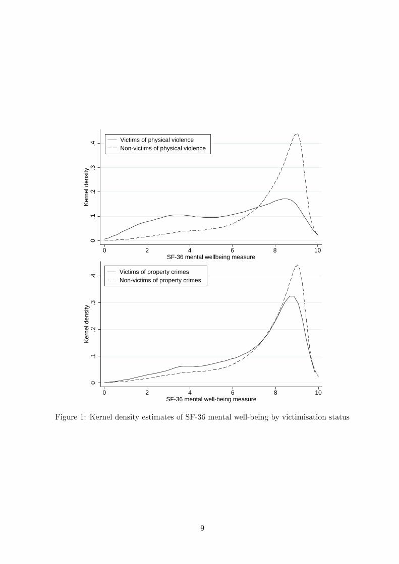
Figure 1 presents the kernel density estimates of the SF-36 mental well-being measure

for each group defined by the type of crime and victimisation status. The two-sample

Kolmogorov-Smirnov test rejects the null hypothesis that the subjective well-being for

victims and non-victims come from the same distribution (p-value=0.000 for both physical

violence and property crimes). Consequently, the distributions of subjective well-being for

crime victims and non-victims are significantly different.

Figure 2 shows that important gaps exist between victims and non-victims at various

percentiles of the well-being distribution. It also shows that the amplitude of these gaps

varies noticeably along the distribution and depending on the type of crime, larger gaps

prevailing for violent crimes. This gives prima facie evidence that the adverse effects of

8

0.1

.2.3

.4K

erne

l den

sity

0 2 4 6 8 10SF-36 mental wellbeing measure

Victims of physical violenceNon-victims of physical violence

kernel = gaussian, bandwidth = 0.5217

Kernel density estimate

0.1

.2.3

.4K

erne

l den

sity

0 2 4 6 8 10SF-36 mental well-being measure

Victims of property crimesNon-victims of property crimes

kernel = gaussian, bandwidth = 0.3510

Figure 1: Kernel density estimates of SF-36 mental well-being by victimisation status

9

victimisation may be felt, to a larger extent, by people at the lower end of the well-being

distribution. This also suggests that focusing on mean estimates does not bring the full

picture of the effects of victimisation. The distributional patterns of subjective well-being

displayed in Figures 1 and 2 motivate us to conduct a distributional analysis of the effects

of physical violence and property crimes on subjective well-being.

02

46

810

SF

-36

men

tal w

ell-b

eing

mea

sure

0 20 40 60 80 100Percentile

Victims of physical violenceNon-victims of physical violence

02

46

810

SF

-36

men

tal w

ell-b

eing

mea

sure

0 20 40 60 80 100Percentile

Victims of property crimesNon-victims of property crimes

Figure 2: SF-36 mental well-being of crime victims and non-victims by percentile

3 Empirical approach

We consider the following equation

SWBit = V ictim1itβ1 + V ictim2itβ2 +X ′itγ + ui + εit (1)

10

where SWBit denotes the subjective well-being of individual i at time t. V ictim1it is an

indicator variable equal to one if an individual is the victim of physical violence and zero

otherwise. V ictim2it indicates whether one is the victim of a property crime or not. Xit is

a vector of control variables typically related with well-being, including age, age squared,

a married dummy, years of schooling, household income, number of family members, and

a dummy variable indicating whether living in a major city. A full set of state of resi-

dence dummies and year dummies are also included. ui denotes the unobserved individual

heterogeneity and εit is the idiosyncratic error term.

We estimate equation (1) with fixed effects (FE) panel estimation. The within estimates

of β1 and β2 separately measure the average effects of physical violence and property

crimes on individual subjective well-being. Compared with OLS estimation, the FE panel

estimation can remove the bias in β1 and β2 due to the unobserved individual heterogeneity

ui.

To explore the heterogeneous effects of crime victimisation along the well-being distri-

bution, we use the panel data quantile regression model with fixed effects (QR–FE) recently

developed by Canay (2011). Modelling fixed effects as location shift variables, Canay (2011)

shows that the QR–FE approach can be carried out in the following two steps. First, we es-

timate the unobserved fixed effects as ui=1T

∑Tt=1(SWBit−V ictim1itβ1−V ictim2itβ2−X ′

itγ),

where β1, β2 and γ are obtained from the FE panel estimation of equation (1). Second, we

implement the standard conditional quantile regression approach of Koenker and Bassett

(1978), using ( SWBit=SWBit−ui) as the dependent variable. More specifically, we solve

the following minimization problem

(β1τ , β2τ , γτ ) = arg min(β1τ ,β2τ ,γτ )

1

NT

N∑i=1

T∑t=1

[ρτ ( SWBit−V ictim1itβ1τ−V ictim2itβ2τ−X ′itγτ )]

(2)

where ρτ (u)=u[τ−I(u<0)] and I is an indicator function. β1τ and β2τ measure separately

the estimated effects of V ictim1it and V ictim2it on the τ -th percentile of the distribution

of SWBit.5

5Interested readers are referred to Canay (2011) for technical details.

11

4 Results

4.1 Victimisation and subjective well-being

Table 2 reports the OLS and FE panel estimates of β1 and β2 in equation (1). Standard

errors reported are corrected for clustering at the individual level.6 The OLS estimates

show that physical violence and property crimes are both significantly associated with

lower levels of mental well-being. On average, physical violence is found to be associated

with a decrease of 0.81 standard deviation (=1.537/1.90) of the SF-36 mental well-being

measure. The mean effect of property crimes is smaller, associated with 0.21 standard

deviation (=0.397/1.90) decline in mental well-being. We further test whether there are

any gender differences in the OLS estimates of the well-being effects of victimisation (Clogg

et al., 1995). We find strong evidence that females are more negatively affected by physical

violence than males, when individual heterogeneity is not accounted for in OLS estimations.

However, OLS estimates suggest no gender differences in the mean well-being effects of

property crimes.

Table 2: Mean effects of victimisation on subjective well-being

All Male Female H0: Male=Female

OLS estimatesPhysical violence –1.537*** –1.231*** –1.776*** p=0.000

(0.081) (0.109) (0.111)

Property crime –0.397*** –0.397*** –0.416*** p=0.790(0.036) (0.050) (0.051)

FE estimatesPhysical violence –0.566*** –0.485*** –0.637*** p=0.193

(0.059) (0.079) (0.086)

Property crime –0.066*** –0.054* –0.078** p=0.603(0.023) (0.030) (0.035)

Note: Control variables include age, age squared, a married dummy, years of schooling,

household income, number of family members, and a dummy variable indicating whether

living in a major city, state of residence dummies and year dummies. Standard errors

clustered at the individual level are reported in parenthesis. * p<0.1; ** p<0.05; ***

p<0.01.

FE estimates are also found to be negative and highly significant but in much smaller

6We use the STATA command qreg2 written by Machado and Santos Silva (2013) (version 3.4, February2015) to perform the estimations. The standard STATA command qreg does not allow us to clusterstandard errors at group level.

12

magnitude than OLS estimates, indicating that ignoring unobserved heterogeneity over-

states the adverse impact of crime victimisation on subjective well-being. On average,

physical violence and property crimes are associated with a decline of respectively 0.30

(=0.566/1.90) and 0.03 (=0.066/1.90) standard deviations of the mental well-being mea-

sure. Consistent with the OLS estimates, the FE estimates of the average negative impact

on mental well-being is still stronger for crimes against the person than for crimes against

property. Furthermore, we cannot find evidence in FE estimates that physical violence has

a stronger effect on the well-being of females than on the well-being of males. Property

crimes are not found to exert differential mean effects on the wellbeing of the two genders.

Table 3: Heterogeneous well-being effects of victimisation (QR–FE estimates)

Q10 Q25 Q50 Q75 Q90

AllPhysical violence –1.089*** –0.852*** –0.549*** –0.248*** –0.054

(0.120) (0.066) (0.019) (0.041) (0.115)

Property crime –0.145*** –0.098*** –0.065*** –0.033** –0.012(0.052) (0.021) (0.008) (0.015) (0.037)

MalePhysical violence –1.135*** –0.752*** –0.454*** –0.229*** –0.057

(0.124) (0.092) (0.048) (0.045) (0.102)

Property crime –0.105* –0.105*** –0.058*** 0.007 –0.008(0.055) (0.026) (0.011) (0.022) (0.038)

FemalePhysical violence –1.180*** –0.955*** –0.580*** –0.258*** –0.081

(0.189) (0.076) (0.021) (0.059) (0.159)

Property crime –0.186*** –0.101*** –0.070*** –0.060** –0.018(0.071) (0.041) (0.012) (0.024) (0.061)

H0: Male=FemalePhysical violence p=0.842 p=0.089 p=0.016 p=0.696 p=0.899

Property crime p=0.367 p=0.934 p=0.461 p=0.040 p=0.889





p<0.01.

Table 3 displays the QR–FE results at the 10th, 25th, 50th, 75th and 90th percentiles

of the distribution of the SF-36 subjective well-being measure. As opposed to the average

case, physical violence has about double the negative impact at the 10th percentile of the

well-being distribution, while the effect is not statistically significant at the 90th percentile.

13

Similarly, we see a monotonic decrease in the detrimental impact of property crimes over the

distribution of subjective well-being. This result corroborates our initial observation that

people at the lower end of the well-being distribution feel the impact of crime to a larger

extent than people at the higher end. It is quite clear that a focus on the average effects

will conceal substantial heterogeneity in the effects of victimisation over the subjective

well-being distribution.

-2.5

-2-1

.5-1

-.5

0Q

R-F

E e

stim

ates

of p

hysi

cal v

iole

nce

0 20 40 60 80 100Percentile

Vitality Social FunctioningRole-Emotional Mental Health

-.5

-.4

-.3

-.2

-.1

0.1

QR

-FE

est

imat

es o

f pro

pert

y cr

imes

0 20 40 60 80 100Percentile

Vitality Social FunctioningRole-Emotional Mental Health

Figure 3: Distributional effects of victimisation on mental well-being components

While we find significant and heterogeneous effects of physical violence and property

crimes on the overall subjective well-being in Tables 2 and 3, it is worth going further and

investigating each component which make up this multifaceted indicator. Indeed, these het-

erogeneous effects may be stronger for some aspects of subjective well-being and weaker for

14

others. For example, among the four constituents of the SF-36 mental well-being measure,

Role-Emotional (RE) measures limitation in work or activities due to emotional health,

while quite differently, Mental Health (MH) measures directly feelings of anxiety and de-

pression. We estimated separately the effects of crime victimisation on each constituent of

SF-36 mental well-being following the same methodology as we did with the overall SF-36,

and illustrate the results at each decile of the well-being distribution in Figure 3.

Consistent with the results reported in Table 3, we find that the effects of physical

violence are heterogeneous for each constituent of mental well-being, with much larger

negative effects at the bottom part of well-being distribution than at the top end. Among

the four constituents, Vitality (VT) is least affected by physical violence throughout the

distribution. Social Functioning (SF) is more negatively affected by physical crimes than

Mental Health (MH). The effects of physical violence on Role-Emotional (RE) show the

greatest heterogeneity among the four components of mental well-being.

We also find dispersed effects of property crimes on each of the four constituents of the

SF-36 mental well-being. Figure 3 shows that the effects of property crimes on Vitality

(VT) and Mental Health (MH) are very similar to each other and are stable along the

well-being distribution. In contrast, property crimes have heterogeneous effects on both

Social Functioning (SF) and Role-Emotional (RE), with greater amplitude at the lower end

of the well-being distribution. Similar to the effects of physical violence, the distributional

effects of property crimes on Role-Emotional (RE) show the greatest heterogeneity among

the four components. In addition, a comparison between physical violence and property

crimes shows that the former has larger adverse consequences throughout the distributions

of the four constituents of mental well-being.

4.2 Subjective well-being effects: victimisation compared with

other life events

In this section, we compare the estimated impact of victimisation with that of other nega-

tive life events which were reported by individuals surveyed in HILDA, namely: (i) serious

personal injury/illness; (ii) fired or made redundant; and (iii) death of spouse or child. Ta-

15

ble 4 shows that 7.80% of the 96,503 observations in our sample reported serious personal

injury/illness in the previous year. About 3.40% of them were fired or made redundant by

employers and 0.59% experienced the death of spouse or children in the past 12 months.

Table 4: Prevalence rates of three other life eventsAll Male FemaleMean SD Mean SD Mean SD

Three other life events(i) Serious personal injury/illness (%) 7.80 0.27 8.09 0.27 7.54 0.26

(ii) Fired or made redundant (%) 3.40 0.18 4.33 0.20 2.61 0.16

(iii) Death of spouse or child (%) 0.59 0.08 0.45 0.07 0.71 0.08

Observations 96,503 45,164 51,339

Note: Data Source: HILDA 2002–2012.

Previous studies have shown that these life events have negative effects on the mean

subjective well-being (Clark et al., 2008; Binder and Coad, 2015). We estimate the effects of

these three life events on SF-36 mental well-being in Australia, using the same methodology

as for victimisation. Table 5 below reports the results.

We find that these three adverse life events all have statistically significant effects

on individual mental well-being. Looking at the mean estimates, the impact of physical

violence on subjective well-being (with an estimated coefficient of –0.566) ranks below that

of personal injuries (–0.706) and the death of spouse or child (–0.728) but is much larger

(about 3 times larger) than the effect of being fired or made redundant (–0.168). On the

opposite, property crimes have a comparatively small mean effect on well-being, ranking

last with an estimated coefficient of –0.066.

However, similar to what we observe with victimisation, we find that these effects are

heterogeneous along the well-being distribution. Their negative impact is mostly felt at

the bottom end of the well-being distribution. So much so that most of the difference

between the impacts of physical violence, personal injury and the death of a spouse or

child occurs below the median of the distribution of well-being. The impact of these life

events estimated at the median and the 75th percentile of the well-being distribution do not

significantly differ from one another. Significant differences reappear at the 90th percentile

where personal injuries and death of a spouse of child still exerting an impact as opposed

16

to physical violence.

Table 5: Well-being effects of other life events (FE and QR–FE estimates)

Mean Q10 Q25 Q50 Q75 Q90

(i) Serious personal injury/illness

All –0.706*** –1.508*** –1.079*** –0.625*** –0.314*** –0.168***(0.024) (0.049) (0.027) (0.018) (0.015) (0.026)

Male –0.667*** –1.591*** –1.018*** –0.572*** –0.268*** –0.131***(0.034) (0.078) (0.041) (0.024) (0.020) (0.038)

Female –0.741*** –1.433*** –1.121*** –0.681*** –0.359*** –0.199***(0.035) (0.060) (0.041) (0.017) (0.023) (0.040)

(ii) Fired or made redundant

All –0.168*** –0.486*** –0.289*** –0.100*** –0.051** 0.028(0.031) (0.068) (0.051) (0.017) (0.020) (0.038)

Male –0.146*** –0.483*** –0.241*** –0.080*** –0.024 0.070(0.038) (0.071) (0.047) (0.019) (0.020) (0.043)

Female –0.204*** –0.524*** –0.362*** –0.133*** –0.020 0.090(0.051) (0.084) (0.044) (0.028) (0.039) (0.055)

(iii) Death of spouse or child

All –0.728*** –1.380*** –1.114*** –0.590*** –0.373*** –0.304**(0.087) (0.131) (0.125) (0.055) (0.071) (0.117)

Male –0.564*** –0.993*** –0.614*** –0.431*** –0.243*** –0.208*(0.116) (0.451) (0.124) (0.066) (0.064) (0.112)

Female –0.873*** –1.566*** –1.225*** –0.717*** –0.432*** –0.435**(0.118) (0.237) (0.141) (0.049) (0.096) (0.212)





p<0.01.

4.3 Robustness checks

4.3.1 Does sample attrition affect the well-being effects of victimisation?

The longitudinal nature of the HILDA Survey allows us to address the bias due to un-

observed individual heterogeneity in our estimations. However, one potential drawback

of using panel estimator is sample attrition. People drop out of the panel survey due to

various reasons such as refusal to respond, death or inability of survey team to locate

them. It could even be that the people worst affected by crime drop out of the survey. If

the characteristics of persons and households that attrite from HILDA are systematically

17

different from those of people who remain, then our analyses that do not account for the

possible selective nature of sample attrition may lead to biased estimates.

The issue of attrition in HILDA is well documented and has been the subject of a

number of studies. Using the first few waves of HILDA, Watson and Wooden (2004)

concur with Fitzgerald et al. (1998) that attrition is likely to affect constant terms rather

than having a significant effect on the coefficient estimates in a regression context, can be

applicable to the HILDA sample. They conclude that “for the first few waves at least, any

bias is likely to be relatively small” (page 307). Further studies by Watson and Wooden

(2006, 2007) find that there is a very large random component to non-response in HILDA

and attrition bias appears to be small. Furthermore, Cai and Waddoups (2011) corroborate

this finding in their analysis of union wage effects using HILDA.

-1.2

-1-.

8-.

6-.

4-.

20

QR

-FE

est

imat

es o

f vic

timiz

atio

n

0 20 40 60 80 100Percentile

Physical violence, not correcting for attrition

Physical violence, correcting for attrition

Property crimes, not correcting for attrition

Property crimes, correcting for attrition

Figure 4: Effects of victimisation, correcting and not correcting for attrition bias

In spite of these encouraging findings, we check whether attrition should be considered

as a problem in the context of our study. We run both our FE and QR–FE models using

the longitudinal weights available in HILDA that can be used to overcome the bias due

to survey non-response and attrition (Watson and Wooden, 2004; Wilkins, 2014). We find

that when the attrition bias has been corrected with sample weights, the FE coefficient

estimates of physical violence and property crimes are very similar to those obtained in

the original models. With regards to whether or not sample attrition affects the QR-FE

coefficients estimates at each decile of the well-being distribution, our results, depicted in

18

Figure 4, show that sample attrition has very trivial effects on our original findings.7

4.3.2 Using alternative measures of subjective well-being

It can be argued that the strong results we have obtained on the effects of crime victim-

isation on individuals’ well-being may be partly due to how we measure well-being. We

test this proposition by using alternative definitions of individuals’ well-being as the de-

pendent variable in the models. In each wave of HILDA, respondents were asked to rate

their overall life satisfaction on a Likert scale of 0 (very dissatisfied) to 10 (very satisfied).

Life satisfaction measure has been used as a measure of general subjective well-being in

many studies such as Clark et al. (2008), Kuroki (2013) and Staubli et al. (2014). Re-

spondents were also asked to report their satisfaction with different domains of life such

as employment opportunities, family relationship, amount of free time, etc. One variable

of particular interest for this study is people’s rating to the question of how safe they feel.

Crime victimisation is highly likely to change people’s subjective feelings of safety. We opt

to use both life satisfaction and safety satisfaction as alternative measures of subjective

well-being in order to check the robustness of our findings.

Table 6 reports the subjective well-being distributions found in HILDA by victimisa-

tion status for the two alternative definitions of subjective well-being. On average, crime

victims are less satisfied with their life and safety than non-victims. A rough comparison

also indicates that physical violence may be more detrimental to people’s happiness than

property crimes. Crime victims have higher propensity to report low levels of life satis-

faction (such as 0, 1, 2, and 3) than non-victims, and they are less likely to report high

levels of life satisfaction (such as 8, 9 and 10). In general, Table 6 shows similar patterns

of subjective well-being distributions of crime victims and non-victims to those revealed in

Figure 1 when subjective well-being is measured through the SF-36 index.

We use life satisfaction and safety satisfaction variables as dependent variables in our

7Using an approach similar to that the one in Cai and Waddoups (2011), we run a FE panel regressionof attrition at time t on victimisation status at t−1, controlling for the covariates used in the subjectivewell-being model. We find no evidence that crime victims are more likely to attrite from the survey thannon-victims, suggesting that the potential bias due to different attrition by victimisation status is probablynot of big concern.

19

Table 6: Subjective well-being distribution by victimisation status (%)

Satisfaction with life Satisfaction with safetyPhysical violence Property crime Physical violence Property crimeYes No Yes No Yes No Yes No

0 1.66 0.08 0.36 0.09 2.13 0.15 0.74 0.15

1 1.20 0.15 0.40 0.16 1.73 0.19 0.91 0.18

2 2.20 0.37 0.70 0.38 2.46 0.45 1.35 0.43

3 3.66 0.70 1.41 0.71 4.66 0.79 2.24 0.78

4 3.26 1.16 2.07 1.15 4.32 1.23 3.21 1.18

5 11.51 4.06 5.68 4.10 9.58 4.15 7.14 4.09

6 10.65 6.19 8.93 6.13 7.58 4.83 6.65 4.78

7 24.68 20.99 23.55 20.92 14.97 14.21 17.34 14.06

8 23.35 35.33 32.00 35.31 22.29 30.24 27.60 30.24

9 11.11 21.28 17.76 21.29 15.90 25.18 19.13 25.34

10 6.72 9.69 7.14 9.77 14.37 18.58 13.69 18.76

Total 100.00 100.00 100.00 100.00 100.00 100.00 100.00 100.00

Mean 6.78 7.83 7.48 7.83 7.01 8.12 7.50 8.13

Observations 1,503 95,000 4,735 91,678 1,503 95,000 4,735 91,678

FE and QR–FE estimations.8 The two dependent variables are categorical variables on

an eleven-point Likert scale (0–10). They can be considered as approximately continuous

and used in quantile regressions. Indeed, using data from the British Household Panel

Survey (BHPS), Binder and Coad (2011, 2015) show that even when their subjective well-

being measure is categorical on a seven-point Likert scale (1–7), quantile regressions can

still uncover heterogeneous effects of covariates on different parts of subjective well-being

distribution.

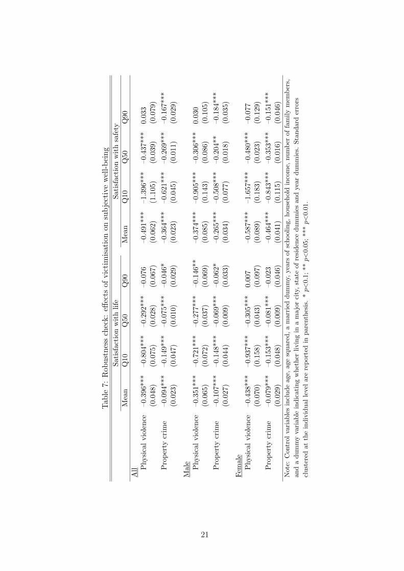
Table 7 reports the FE and QR–FE estimates. We find very similar results to those

reported in Tables 3 and 4. The main findings are: (i) On average, both physical violence

and property crimes reduce people’s satisfaction with life, and we find the average negative

impact on life satisfaction to be much stronger for crimes against the person than for

crimes against property; (ii) The effects of physical violence and property crimes are highly

8One concern of using measures of this type is their interpersonal comparability, as survey respondentsmay interpret and use the response categories differently (Ng, 1997). When using the FE and QR–FEestimation, we do not need to assume that the answers to satisfaction questions are fully interpersonallycomparable because the individual fixed effects (ui) can adequately deal with this issue. In addition, theuse of the linear specification assumes cardinality in satisfaction answers, which means that we have toassume that the difference in satisfaction between a three and a four for any individual is the same asbetween a five and a six for any other individual. Ferrer-i Carbonell and Frijters (2004) find that cardinalityassumption generally does not lead to different conclusions.

20

Tab

le7:

Rob

ust

nes

sch

eck:

effec

tsof

vic

tim

isat

ion

onsu

bje

ctiv

ew

ell-

bei

ng

Sat

isfa

ctio

nw

ith

life

Sat

isfa

ctio

nw

ith

safe

tyM

ean

Q10

Q50

Q90

Mea

nQ

10Q

50Q

90

All P

hysi

cal

vio

len

ce–0

.396

***

–0.8

04**

*–0

.292

***

–0.0

76–0

.491

***

–1.3

96**

*–0

.437

***

0.03

3(0

.048)

(0.0

75)

(0.0

28)

(0.0

67)

(0.0

62)

(1.1

05)

(0.0

39)

(0.0

79)

Pro

per

tycr

ime

–0.0

94**

*–0

.149

***

–0.0

75**

*–0

.046

*–0

.364

***

–0.6

21**

*–0

.269

***

–0.1

67**

*(0

.023)

(0.0

47)

(0.0

10)

(0.0

29)

(0.0

23)

(0.0

45)

(0.0

11)

(0.0

29)

Male Physi

cal

vio

len

ce–0

.351

***

–0.7

21**

*–0

.277

***

–0.1

46**

–0.3

74**

*–0

.905

***

–0.3

06**

*0.

030

(0.0

65)

(0.0

72)

(0.0

37)

(0.0

69)

(0.0

85)

(0.1

43)

(0.0

86)

(0.1

05)

Pro

per

tycr

ime

–0.1

07**

*–0

.148

***

–0.0

69**

*–0

.062

*–0

.265

***

–0.5

08**

*–0

.204

**–0

.184

***

(0.0

27)

(0.0

44)

(0.0

09)

(0.0

33)

(0.0

34)

(0.0

77)

(0.0

18)

(0.0

35)

Fem

ale

Physi

cal

vio

len

ce–0

.438

***

–0.9

37**

*–0

.305

***

0.00

7–0

.587

***

–1.6

57**

*–0

.480

***

–0.0

77(0

.070)

(0.1

58)

(0.0

43)

(0.0

97)

(0.0

89)

(0.1

83)

(0.0

23)

(0.1

29)

Pro

per

tycr

ime

–0.0

79**

*–0

.153

***

–0.0

81**

*–0

.023

–0.4

64**

*–0

.843

***

–0.3

53**

*–0

.151

***

(0.0

29)

(0.0

48)

(0.0

09)

(0.0

46)

(0.0

41)

(0.1

15)

(0.0

16)

(0.0

46)

Not

e:C

ontr

olva

riab

les

incl

ud

eag

e,ag

esq

uare

d,

am

arr

ied

du

mm

y,ye

ars

of

sch

ooli

ng,

hou

seh

old

inco

me,

nu

mb

erof

fam

ily

mem

ber

s,

and

ad

um

my

vari

able

ind

icat

ing

wh

eth

erli

vin

gin

am

ajo

rci

ty,

state

of

resi

den

ced

um

mie

san

dye

ar

du

mm

ies.

Sta

nd

ard

erro

rs

clu

ster

edat

the

ind

ivid

ual

leve

lar

ere

por

ted

inp

are

nth

esis

.*p<

0.1

;**p<

0.0

5;

***p<

0.0

1.

21

heterogeneous with much larger impact in the lower part of the life satisfaction distribution

than at the higher end; (iii) Both physical violence and property crimes affect people’s

happiness with safety negatively, and the impact decreases along the distribution of safety

satisfaction; and (iv) Physical violence and property crimes adverseimpact satisfaction with

safety to a larger extent than for life satisfaction. One possible explanation for this finding

is that the overall life satisfaction is a global conception of well-being that aggregates

the happiness with different domains of life (van Praag et al., 2003), and happiness with

safety, one of the many domains of life, is a very important channel through which crimes

victimisation affects life satisfaction.9

4.3.3 Have individuals experienced declined subjective well-being before vic-

timisation?

Although our estimations address the endogeneity bias arising from unobserved individ-

ual heterogeneity, they cannot address the bias that could arise from the possible reverse

causality between crime victimisation and subjective well-being. If individuals who have

experienced a negative shock to subjective well-being are more likely to become victims

of crimes, then we may have overestimated the negative consequences of crime victimi-

sation for subjective well-being. In this section, we test whether we observe significant

declines in subjective well-being prior to crime victimisation. Namely, we test whether

crime victimisation is a predictable event or not.10

We run FE panel regressions of subjective well-being measures on a set of dummy

9To assess the degree to which the negative effect of victimisation on happiness can be explained by theassociated declines in happiness with safety, we re-estimate the life satisfaction equation using satisfactionwith safety as an additional control in the FE and QR–FE regressions. We find around one third of theaverage negative effect of physical violence on life satisfaction can be attributed to its negative impacton feelings of safety. Throughout the distribution of life satisfaction, the rising feelings of insecurity afterphysical violence can explain about 16% to 38% of the declines in life satisfaction. In contrast, the mean anddistributional effects of property crimes on life satisfaction become insignificant after controlling for safetysatisfaction, suggesting that the decreasing subjective well-being due to property crimes are solely driven bythe deteriorating happiness about safety. A note of caution needs to be issued regarding the above findingsas safety satisfaction is an endogenous variable when included in life satisfaction estimation. Ideally, wewant to address the endogeneity problem of safety satisfaction using instrumental variable estimation. Avalid instrument that is highly correlated with safety satisfaction but not correlated with life satisfactionis unavailable in HILDA.

10The approach we take here is similar to the ones used in Clark et al. (2008) and Cornaglia et al. (2014)for examining the dynamic well-being effects of life events.

22

Tab

le8:

Dynam

icw

ell-

bei

ng

effec

tsof

vic

tim

isat

ion

SF

-36

men

tal

wel

l-b

ein

gS

atis

fact

ion

wit

hO

vera

llV

TS

FR

EM

Hli

fesa

fety

Physicalviolence

Th

ree

orm

ore

year

sb

efore

0.11

70.

007

0.12

40.

350

–0.0

110.

061

0.18

5(t–(3+))

(0.1

25)

(0.1

11)

(0.1

65)

(0.2

46)

(0.1

07)

(0.0

95)

(0.1

16)

Tw

oye

ars

bef

ore

–0.0

02–0

.065

0.04

70.

065

–0.0

54–0

.016

–0.0

02(t–2)

(0.1

14)

(0.0

99)

(0.1

48)

(0.2

26)

(0.1

00)

(0.0

99)

(0.1

22)

On

eye

ar

bef

ore

(referen

ce)

——

——

——

—(t–1)

Yea

rof

vic

tim

isati

on

–0.5

49**

*–0

.230

***

–0.6

51**

*–0

.788

***

–0.5

27**

*–0

.400

***

–0.5

68**

*(t)

(0.1

01)

(0.0

85)

(0.1

26)

(0.1

91)

(0.0

94)

(0.0

83)

(0.1

04)

On

eye

ar

afte

r–0

.163

*–0

.143

*–0

.199

*–0

.195

–0.1

16–0

.106

–0.0

76(t+1)

(0.0

95)

(0.0

84)

(0.1

16)

(0.1

97)

(0.0

84)

(0.0

85)

(0.0

92)

Tw

oye

ars

afte

r–0

.166

–0.0

67–0

.243

*–0

.284

–0.0

68–0

.133

–0.0

79(t+2)

(0.1

03)

(0.0

89)

(0.1

25)

(0.2

11)

(0.0

94)

(0.0

93)

(0.1

14)

Th

ree

orm

ore

year

saft

er–0

.012

–0.0

910.

053

0.01

3–0

.023

–0.1

17–0

.140

(t+(3+))

(0.1

23)

(0.1

08)

(0.1

50)

(0.2

43)

(0.1

07)

(0.0

98)

(0.1

28)

Propertycrim

es

Th

ree

orm

ore

year

sb

efore

0.01

4–0

.036

–0.0

670.

144

0.01

40.

007

0.05

2(t–(3+))

(0.0

55)

(0.0

55)

(0.0

71)

(0.1

12)

(0.0

51)

(0.0

46)

(0.0

51)

Tw

oye

ars

bef

ore

–0.0

32–0

.081

*0.

035

–0.0

920.

008

–0.0

290.

020

(t–2)

(0.0

45)

(0.0

44)

(0.0

60)

(0.0

90)

(0.0

42)

(0.0

36)

(0.0

43)

On

eye

ar

bef

ore

(referen

ce)

——

——

——

—(t–1)

Yea

rof

vic

tim

isati

on

–0.0

54–0

.048

–0.0

36–0

.080

–0.0

53–0

.089

**–0

.350

***

(t)

(0.0

41)

(0.0

40)

(0.0

56)

(0.0

81)

(0.0

37)

(0.0

35)

(0.0

45)

On

eye

ar

afte

r0.

007

–0.0

020.

006

0.01

20.

012

0.02

1–0

.032

(t+1)

(0.0

44)

(0.0

41)

(0.0

58)

(0.0

89)

(0.0

38)

(0.0

33)

(0.0

41)

Tw

oye

ars

afte

r–0

.010

–0.0

120.

007

–0.0

450.

011

–0.0

34–0

.047

(t+2)

(0.0

46)

(0.0

44)

(0.0

59)

(0.0

89)

(0.0

42)

(0.0

36)

(0.0

43)

Th

ree

orm

ore

year

saft

er0.

036

0.03

60.

024

0.03

40.

051

0.00

7–0

.034

(t+(3+))

(0.0

55)

(0.0

54)

(0.0

71)

(0.1

07)

(0.0

49)

(0.0

42)

(0.0

51)

Not

e:C

ontr

olva

riab

les

incl

ud

eag

e,ag

esq

uare

d,

am

arr

ied

du

mm

y,ye

ars

of

sch

ooli

ng,

hou

seh

old

inco

me,

nu

mb

erof

fam

ily

mem

ber

s,

and

ad

um

my

vari

able

ind

icat

ing

wh

eth

erli

vin

gin

am

ajo

rci

ty,

state

of

resi

den

ced

um

mie

san

dye

ar

du

mm

ies.

Sta

nd

ard

erro

rs

clu

ster

edat

the

ind

ivid

ual

leve

lar

ere

por

ted

inp

are

nth

esis

.*p<

0.1

;**p<

0.0

5;

***p<

0.0

1.

23

variables indicating one year, two years, three and more years before and after the year

when crime victimisation happened. The logic of our approach is that if there is a decline

in subjective well-being prior to crime victimisation, the well-being effect of the dummy

indicating two years prior to victimisation (t−2) on mental well-being (at time t) should

be statistically different from the well-being effect of the dummy indicating one year before

victimisation (t−1). Among all the year dummies, we select the dummy indicating one

year before the victimisation (t−1) as the reference category. To our purpose of detecting

whether there is a drop in subjective well-being before victimisation happens, we only

need to test whether the estimated coefficient of year dummy (t−2) has a positive sign and

whether it is statistically significant.

Table 8 report the results of these tests. We find no evidence, on both types of well-being

measures, that the coefficient on (t−2) dummy is both positive and statistically significant

(relative to the reference (t−1) dummy). Thus, we find no evidence that people’s subjective

well-being becomes significantly lower prior to victimisation. What makes this conclusion

more convincing is that the coefficient estimate of the year dummy indicating three or

more years before the incident (t−(3+)) is also not statistically significant. This finding

corroborates the previous speculations by Powdthavee (2005), Davies and Hinks (2010)

and Staubli et al. (2014) that it is intuitively implausible that subjective well-being affects

victimisation in an adult population.

Consistent with our expectation, Table 8 shows that there is a significant difference

in subjective well-being between the year prior to victimisation and the year of victim-

isation. The dynamic results provided in Table 8 indicate the negative impact of crime

victimisation on subjective well-being is transitory. Crime victims experience a significant

decline in subjective well-being throughout year following victimisation. They then will

restore to pre-victimisation level one year after the event. Using data from the German

Socio-Economic Panel, Clark et al. (2008) examine the dynamic effects of many life events

such as marriage, divorce, widowhood, child birth and layoff on people’s life satisfaction

and they find evidence of complete adaptation to these life events in a short time span. We

find similar evidence of adaptation in people’s subjective well-being to crime victimisation.

24

5 Conclusion

This paper estimates the effects of crime victimisation on subjective well-being, using data

from the longitudinal Household, Income and Labour Dynamics in Australia (HILDA)

survey. Using fixed effects panel estimations, our analysis shows that both physical violence

and property crimes negatively affect the subjective well-being of Australians. We find

that the average effect is much stronger for physical violence than for property crimes. On

average, physical violence and property crimes are associated with a decline of respectively

0.30 and 0.03 standard deviation on the SF-36 mental well-being scale. Using recently

developed panel data quantile regression model with fixed effects, we find strong evidence

of heterogeneous links between crime victimisation and happiness. The adverse effects of

both physical violence and property crimes are most strongly felt at the lower end of the

distribution of well-being.

Comparing the well-being effects of physical attacks and property crimes with three

other life events (i) serious personal injury/illness; (ii) fired or made redundant; and (iii)

death of spouse or child, we find that physical violence is much more distressing than

being fired. While we find the mean effect of violent crimes to be smaller than that of

personal injury/illness and the death of a spouse or child, we also find that these three life

events are much closer than originally seems when one accounts for the heterogeneity of

the effects along the well-being distribution. Indeed, most of the differences are observed in

lower deciles of the distribution where the effects are stronger while the magnitude of the

effects is much more concentrated above the median of the distribution. Accounting for the

distributional heterogeneity of the effects of crime illustrates the highly damaging effect of

violent crimes on people at the lower end of the well-being distribution. By contrast, we

find that the distributional negative well-being effects of property crimes to be relatively

small.

Our findings of adverse effects of victimisation on subjective wellbeing are robust to

(i) the correction of sample attrition in HILDA and (ii) the usage of alternative well-being

measures (life satisfaction and safety satisfaction) as dependent variables. Furthermore, we

cannot find evidence that the negative well-being effects of crime victimisation are driven

25

by reverse causality (in which case people may experience a negative shock to subjective

well-being before becoming crime victims).

An important result of this study is that the negative effects of crime on well-being are

intense but short-lived, to an extent that is similar to all other negative (and positive) life

events (Clark et al., 2008). People adapt. However, this is not to say that before they do

adapt, the adverse consequences of crime on well-being are likely to snowball into further

negative outcomes, having themselves further consequences on individuals’ well-being. For

instance, using the same data, Fritjers et al. (2014) find that a one standard deviation

decrease in mental health leads to 30 percentage point decrease in employment. We do

find that violent crime decreases well-being by 0.30 standard deviation, suggesting that the

employment effect of experiencing violent crimes may be in the magnitude of 10 percentage

points.

The findings reported in this paper have important policy implications. Non-pecuniary

costs of crime such as psychological well-being losses of victims should be taken into con-

sideration by policy makers, in addition to pecuniary costs such as financial losses and

medical expenses. From the policy perspective, the consideration of the previously unmea-

sured cost of crime strengthens the case for public spending to combat crime. Furthermore,

crime leads to important shocks to individual subjective well-being which could be offset,

would victims be provided with adequate professional support following such traumatic life

events. This is an area where public policy can potentially increase its involvement over

and beyond its usual roles of crime prevention and financially compensating victims.

References

Atkeson, B. M., K. S. Calhoun, P. A. Resick, and E. M. Ellis (1982). “Victims of rape:

Repeated assessment of depressive symptoms”. Journal of Consulting and Clinical Psy-

chology 50, 96–102.

Binder, M. and A. Coad (2011). “From Average Joe’s happiness to Miserable Jane and

26

Cheerful John: using quantile regressions to analyze the full subjective well-being dis-

tribution”. Journal of Economic Behavior & Organization 79, 275–290.

Binder, M. and A. Coad (2015). “Heterogeneity in the relationship between unemploy-

ment and subjective well-being: A quantile approach”. Economica, forthcoming. Doi:

10.1111/ecca.12150.

Cai, L. and J. Waddoups (2011). “Union wage effects in Australia: Evidence from panel

data”. British Journal of Industrial Relations 49, s279–s305.

Canay, A. I. (2011). “A simple approach to quantile regression for panel data”. Econo-

metrics Journal 14, 368–386.

Chatterji, P., M. Alegria, M. Lu, and D. Takeuchi (2007). “Psychiatric disorders and labor

market outcomes: Evidence from the National Latino and Asian American Study”.

Health Economics 16, 1069–1090.

Chatterji, P., M. Alegria, and D. Takeuchi (2011). “Psychiatric disorders and labor market

outcomes: Evidence from the National Comorbidity Survey-Replication”. Journal of


Clark, A. E., E. Diener, Y. Georgellis, and R. E. Lucas (2008). “Lags and leads in life

satisfaction: A test of the baseline hypothesis”. Economic Journal 118, F222–F243.

Clogg, C. C., E. Petkova, and A. Haritou (1995). “Statistical methods for comparing

regression coefficients between models”. American Journal of Sociology 100, 1261–1293.

Cohen, M. A. (2008). “The effect of crime on life satisfaction”. Journal of Legal Studies 37,

S325–S353.

Cornaglia, F., N. E. Feldman, and A. Leigh (2014). “Crime and mental well-being”. Journal

of Human Resources 49, 110–140.

Davies, S. and T. Hinks (2010). “Crime and happiness amongst heads of households in

Malawi”. Journal of Happiness Studies 11, 457–476.

27

Davis, R. and L. Friedman (1985). “The emotional aftermath of crime and violence”. In

C. Figley (Ed.), Trauma and Its Wake: The Study and Treatment of Post-traumatic

Stress Disorder. New York: Brunner/Mazel.

Dustmann, C. and F. Fasani (2015). “The effect of local area crime on mental health”.

Economic Journal , forthcoming. Doi: 10.1111/ecoj.12205.

Ferrer-i Carbonell, A. and P. Frijters (2004). “How important is methodology for the

estimates of the determinants of happiness?”. Economic Journal 114, 641–659.

Fitzgerald, J., P. Gottschalk, and R. Moffitt (1998). “An analysis of sample attrition

in panel data: The Michigan Panel Study of Income Dynamics”. Journal of Human

Resources 33, 251–299.

Flatau, P., J. Galea, and R. Petridis (2000). “Mental health and wellbeing and unemploy-

ment”. Australian Economic Review 2, 161–181.

Fritjers, P., D. W. Johnston, and M. A. Shields (2014). “The effect of mental health on

employment: Evidence from Australian panel data”. Health Economics 23, 1058–1071.

Hamilton, V. H., P. Merrigan, and E. Dufresne (1997). “Down and out: estimating the

relationship between mental health and unemployment”. Health Economics 6, 397–406.

Hanslmaier, M. (2013). “Crime, fear and subjective well-being: How victimization and

street crime affect fear and life satisfaction”. European Journal of Criminology 10, 515–

533.

Hays, R., C. Sherbourne, and R. Mazel (1993). “The rand 36-item health survey 1.0”.


Hemingway, H., M. Stafford, S. Stansfeld, M. Shipley, and M. Marmot (1997). “Is the

SF-36 a valid measure of change in population health? Results from the Whitehall II

Study”. British Medical Journal 315, 1273–1279.

Koenker, R. and G. Bassett (1978). “Regression quantiles”. Econometrica 46, 33–50.

28

Kuroki, M. (2013). “Crime victimization and subjective well-being: Evidence from happi-

ness data”. Journal of Happiness Studies 14, 783–794.

Machado, J. and J. Santos Silva (2013). “Quantile regression and heteroskedasticity”.

Working paper.

Moller, V. (2005). “Resilient or resigned? Criminal victimization and quality of life in

South Africa”. Social Indicators Research 72, 263–317.

Moore, S. C. (2006). “The value of reducing fear: An analysis using the European Social

Survey”. Applied Economics 38, 115–117.

Ng, Y. (1997). “A case for happiness, cardinalism, and interpersonal comparability”.

Economic Journal 107, 1848–1858.

Norris, F. and K. Kaniasty (1992). “A longitudinal study of the effects of various crime

prevention strategies on criminal victimization, fear of crime, and psychological distress”.

American Journal of Community Psychology 20, 625–648.

OECD (2010). OECD Factbook 2009. Paris: Organisation for Economic Co-operation and

Development (OECD).

Ojeda, V. D., R. G. Frank, T. G. McGuire, and T. P. Gilmer (2010). “Mental illness,

nativity, gender and labor supply”. Health Economics 19, 396–421.

Powdthavee, N. (2005). “Unhappiness and crime: Evidence from South Africa”. Econom-

ica 72, 531–547.

Ross, C. (1993). “Fear of victimization and health”. Journal of Quantitative Criminology 9,

159–175.

Staubli, S., M. Killias, and B. S. Frey (2014). “Happiness and victimization: An empirical

study for Switzerland”. European Journal of Criminology 11, 57–72.

van Praag, B., P. Frijters, and A. F. i Carbonell (2003). “The anatomy of subjective

well-being”. Journal of Economic Behavior & Organization 51, 29–49.

29

Watson, N. and M. Wooden (2004). “Sample attrition in the HILDA survey”. Australian

Journal of Labour Economics 7, 293–308.

Watson, N. and M. Wooden (2006). “Identifying factors affecting longitudinal survey

response”. Paper Presented at the Methodology of Longitudinal Surveys Conference,

University of Essex, Colchester, UK, 12–14 July.

Watson, N. and M. Wooden (2007). “The HILDA Survey and its contribution to economic

and social research (so far)”. Economic Record 83, 208–231.

Wilkins, R. (2014). Families, Incomes and Jobs,Volume 9: A Statistical Report on Waves

1 to 11 of the Household, Income and Labour Dynamics in Australia Survey. Melbourne

Institute of Applied Economic and Social Research, University of Melbourne.

30

crime victimisation and subjective well-being: panel ...ftp.iza.org/dp9253.pdf · discussion paper...

Documents